Page 1
Master's Degree Thesis ISRN: BTH-AMT-EX--2012/D-05--SE
Supervisors: Johan Wall, BTH
Department of Mechanical Engineering Blekinge Institute of Technology
Karlskrona, Sweden
2012
Amir Partovi
Saadat Sharifi Shamili
Analysis of autofrettaged high pressure components
Page 3
Analysis of autofrettaged high
pressure components
Amir Partovi
Saadat Sharifi Shamili
Department of Mechanical Engineering
Blekinge Institute of Technology
Karlskrona, Sweden
2012
Thesis submitted for completion of Master of Science in Mechanical
Engineering with emphasis on Structural Mechanics at the Department of
Mechanical Engineering, Blekinge Institute of Technology, Karlskrona,
Sweden.
Abstract
Autofrettage is a procedure performed to improve the durability of high
pressure components. The main aim of this thesis work was to analyse
the effect of autofrettage on the valve house of the cutting head
assembly of a water jet cutting machine. As the stepping stone, a thick
pipe, as a typical example of pressure vessels, was employed in order to
study autofrettage process and its effects. Afterward, the adopted
approach was applied on the valve house. Eventually, the results showed
that this procedure leads to a tangible decrease in the maximum value of
stress.
Keywords
Autofrettage, Residual Stress, Hoop stress, Plasticity, Hardening,
ABAQUS.
Page 4
2
Acknowledgement
This thesis was carried out at the Department of Mechanical Engineering,
Blekinge Institute of Technology, Karlskrona, Sweden, under the
supervision of Dr. Johan Wall, in order to fulfill the Master’s Programme in
Mechanical Engineering with emphasis on Structural Mechanics.
The thesis was a part of research project defined by the Swedish Waterjet
laboratory (SWL) in Ronneby, Sweden which is a research centre organized
by Blekinge Institute of Technology. This thesis work was initiated in
February 2012.
We wish to express our great appreciation toward Dr. Johan Wall for his
supportive supervision and guidance during the process of this thesis work.
Also, we would like to thank Dr. Sharon Kao-Walter for her support during
the experimental material testing as well as Dr. Ansel Berghuvud for his
efforts during the whole programme.
Last but not the least, we would like to thank Mr. Mansour Partovi for his
effort and support to provide the test specimens.
Karlskrona, August 2012
Amir Partovi
Saadat Sharifi Shamili
Page 5
3
Contents
1. Notations ................................................................................................. 5
2. Introduction ............................................................................................ 7
2.1. Background ....................................................................................... 7
2.2. Aim.................................................................................................... 9
2.3. Method ............................................................................................ 10
3. Valve house and its role in the cutting head assembly ...................... 12
4. Autofrettage procedure ....................................................................... 16
4.1. An introduction to autofrettage and its benefits .............................. 16
4.2. Analytical study of stress distribution ............................................. 19
4.2.1. Stress components before autofrettage ..................................... 20
4.2.2. Radial displacement before autofrettage ................................... 22
4.2.3. Stress components after autofrettage ........................................ 22
4.3. A brief introduction to plasticity ..................................................... 23
4.3.1. Yield criteria and yield surfaces ........................................... 25
4.3.2. Bauschinger effect ................................................................ 27
4.3.3. Models of plasticity .............................................................. 27
4.4. Source of nonlinearity in this study ................................................ 30
5. Autofrettage in Abaqus ....................................................................... 32
Page 6
4
5.1. Autofrettage analysis of the pipe ..................................................... 33
5.1.1. Verification of the pipe model .............................................. 34
5.1.2. Autofrettage of the pipe......................................................... 41
5.1.3. Results of the autofrettage analysis of the pipe ..................... 49
5.1.3.1 Minimum and maximum of the autofrettage pressure ........ 53
5.1.3.2. Radius of plasticity ............................................................. 58
5.1.3.3. Residual stresses ................................................................. 62
5.2. Autofrettage analysis of the valve house ......................................... 67
5.2.1. Preparing a 3D study ............................................................. 67
5.2.2. Autofrettage of the valve house ............................................ 72
5.2.3. Results of the autofrettage analysis of the valve house ......... 74
5.2.3.1. Bigger working pressure, the same maximum VMS ......... 78
5.2.3.2. Effect of different number of stages in autofrettage .......... 80
6. Conclusion and future works .............................................................. 82
6.1. Conclusion and discussion .............................................................. 82
6.2. Future works .................................................................................... 84
7. References ............................................................................................. 85
Appendix .................................................................................................... 87
A. Stress distribution in a thick walled cylinder ..................................... 87
B. Displacement in a thick walled cylinder ............................................ 90
C. Stress distribution after autofrettage .................................................. 90
Page 7
5
1. Notations
E Modulus of elasticity
F Axial force
k Ratio of outer to inner radius
n Strain hardening exponent
P pressure
Py1 Minimum of autofrettage pressure
Py2 Maximum of autofrettage pressure
r radius
T Temperature
u Radial displacement
v Circumferential displacement
w Axial displacement
α Thermal linear expansion coefficient
ε Strain
εe Elastic strain
εp Plastic strain
εr Radial strain
εT Total strain
εz Axial strain
Page 8
6
εθ Circumferential strain
ν Poisson’s ratio
σ Stress
σ1 Principal radial stress
σ2 Principal circumferential stress
σ3 Principal axial stress
σr Radial stress
σt, σθ Circumferential stress
σz Axial stress
ϕa, ϕn Auxiliary variables
Indices
A Autofrettage
i Inner
Nom Nominal
o Outer
T Tresca
VM Von Mises
W Working
y Yield
Page 9
7
2. Introduction
2.1. Background
Pressure vessels are leak proof containers that are used to store, transfer and
process of the fluids in a condition of unusual pressure and/or temperature;
obviously, they play a vital role in many industrial settings. The importance
of pressure vessels has arisen to the efforts in order to have an appropriate
understanding of the stress distribution of the structure of pressure vessels
due to the extraordinary amount of pressure that they need to withstand.
Beside this, the need for pressure vessels that can undergo much higher
pressure levels has inspired the innovation of new techniques in the field of
pressure vessels (Harvey [1]).
Figure 2.1. Different types of pressure vessels
A very common type of pressure vessels are thick walled cylinders. Mainly,
there are three methods that can be chosen in order to reinforce a thick
Page 10
8
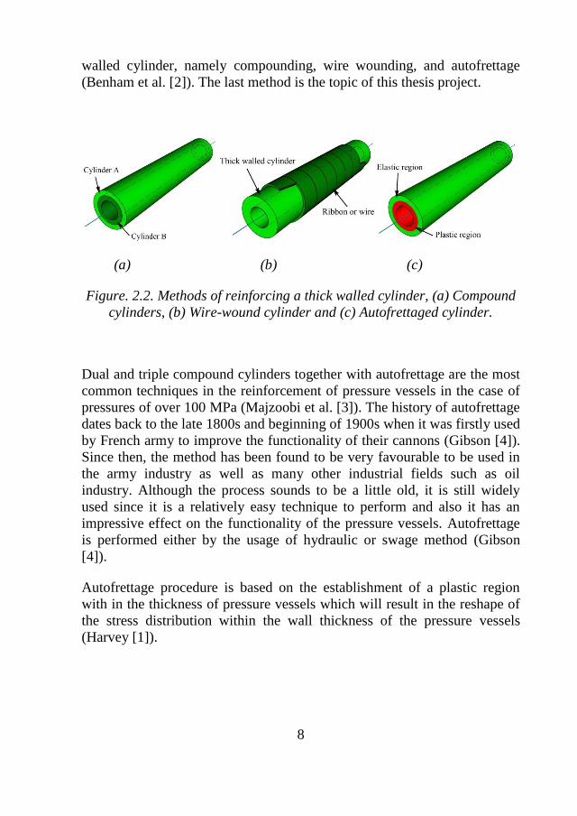
walled cylinder, namely compounding, wire wounding, and autofrettage
(Benham et al. [2]). The last method is the topic of this thesis project.
(a) (b) (c)
Figure. 2.2. Methods of reinforcing a thick walled cylinder, (a) Compound
cylinders, (b) Wire-wound cylinder and (c) Autofrettaged cylinder.
Dual and triple compound cylinders together with autofrettage are the most
common techniques in the reinforcement of pressure vessels in the case of
pressures of over 100 MPa (Majzoobi et al. [3]). The history of autofrettage
dates back to the late 1800s and beginning of 1900s when it was firstly used
by French army to improve the functionality of their cannons (Gibson [4]).
Since then, the method has been found to be very favourable to be used in
the army industry as well as many other industrial fields such as oil
industry. Although the process sounds to be a little old, it is still widely
used since it is a relatively easy technique to perform and also it has an
impressive effect on the functionality of the pressure vessels. Autofrettage
is performed either by the usage of hydraulic or swage method (Gibson
[4]).
Autofrettage procedure is based on the establishment of a plastic region
with in the thickness of pressure vessels which will result in the reshape of
the stress distribution within the wall thickness of the pressure vessels
(Harvey [1]).
Page 11
9
2.2. Aim
One of the modern applications of the autofrettage technique is in the so
called “water jet cutting” technology. The idea of this modern technology is
to use the energy of pressurized water in order to cut different materials.
Obviously, there are many parts in a water jet machine that should be able
to withstand a very high pressure for thousands of working cycles.
The main aim of this project is to suggest an appropriate model that can
provide a reliable study of autofrettage effect on an important part of the
water jet cutting machine namely, the valve house of the cutting head
assembly.
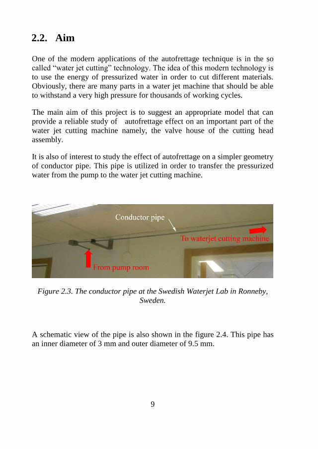
It is also of interest to study the effect of autofrettage on a simpler geometry
of conductor pipe. This pipe is utilized in order to transfer the pressurized
water from the pump to the water jet cutting machine.
Figure 2.3. The conductor pipe at the Swedish Waterjet Lab in Ronneby,
Sweden.
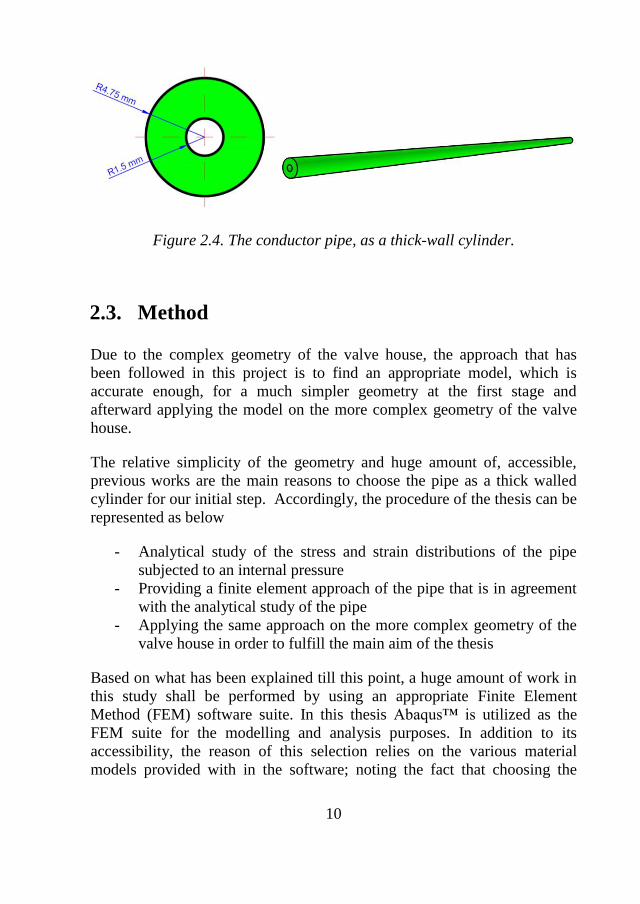
A schematic view of the pipe is also shown in the figure 2.4. This pipe has
an inner diameter of 3 mm and outer diameter of 9.5 mm.
Page 12
10
Figure 2.4. The conductor pipe, as a thick-wall cylinder.
2.3. Method
Due to the complex geometry of the valve house, the approach that has
been followed in this project is to find an appropriate model, which is
accurate enough, for a much simpler geometry at the first stage and
afterward applying the model on the more complex geometry of the valve
house.
The relative simplicity of the geometry and huge amount of, accessible,
previous works are the main reasons to choose the pipe as a thick walled
cylinder for our initial step. Accordingly, the procedure of the thesis can be
represented as below
- Analytical study of the stress and strain distributions of the pipe
subjected to an internal pressure
- Providing a finite element approach of the pipe that is in agreement
with the analytical study of the pipe
- Applying the same approach on the more complex geometry of the
valve house in order to fulfill the main aim of the thesis
Based on what has been explained till this point, a huge amount of work in
this study shall be performed by using an appropriate Finite Element
Method (FEM) software suite. In this thesis Abaqus™ is utilized as the
FEM suite for the modelling and analysis purposes. In addition to its
accessibility, the reason of this selection relies on the various material
models provided with in the software; noting the fact that choosing the
Page 13
11
suitable material model has a vital role in the procedure of this thesis work.
Beside this, the ease of use, as well as CAD (Computer Aided Design)
abilities of the software have been other motivations of this choice. This
method is also shown in the following flowchart.
Yes
No
Start
Are results
the same?
Choosing appropriate model and Applying autofrettage
pressure
Obtaining and validation of the results
Utilizing the same approach for the valve house
Analytical study of the pipe; considering just elastic condition
Numerical study of the pipe; creating a model and applying a
relatively low pressure
Modification
Obtaining the results
End
Page 14
12
3. Valve house and its role in the cutting
head assembly
As it is clarified in the previous chapter, the main aim of this thesis job is to
present the effects of autofrettage on an important part of a waterjet cutting
machine. This part is the valve house of the cutting head assembly.
Accordingly, it is necessary to have an understanding of this part and its
functionality; this issue is addressed in this chapter. Figure 3.1 shows the
location of cutting head assembly within the waterjet cutting machine.
Figure 3.1. The waterjet cutting machine and the place of its cutting head
assembly.
Page 15
13
Different parts of the cutting head assembly are shown in the below figure
in which the location of the valve house is indicated.
Figure 3.2. The cutting head assembly and its components.
As it is illustrated in the figure 3.2, the pressurized water enters the valve
house. In this stage, a pneumatic actuator controls the open and close
positions and the outlet water, after passing an orifice, is mixed with an
appropriate abrasive and finally exits through the nozzle.
Page 16
14
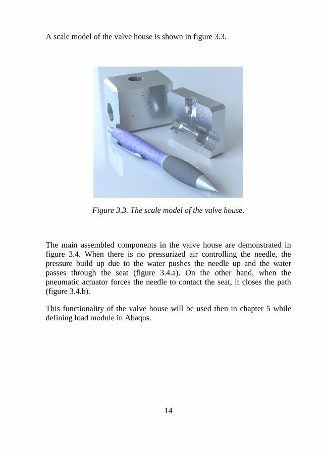
A scale model of the valve house is shown in figure 3.3.
Figure 3.3. The scale model of the valve house.
The main assembled components in the valve house are demonstrated in
figure 3.4. When there is no pressurized air controlling the needle, the
pressure build up due to the water pushes the needle up and the water
passes through the seat (figure 3.4.a). On the other hand, when the
pneumatic actuator forces the needle to contact the seat, it closes the path
(figure 3.4.b).
This functionality of the valve house will be used then in chapter 5 while
defining load module in Abaqus.
Page 17
15
(a)
(b)
Figure 3.4. The cut view of the valve house in the open and close positions.
Page 18
16
4. Autofrettage procedure
4.1. An introduction to autofrettage and its benefits
In this section, a concise discussion regarding the necessity of the
autofrettage and the principles of its functioning is provided. The current
discussion focuses on the autofrettage of the pipe as a thick walled cylinder;
however the principles that are explained here can easily be generalized to
the autofrettage of any other geometry.
As it will be discussed in the upcoming section an arbitrary element within
the cross section of a thick walled cylinder is subjected to the biaxial stress
condition (Boresi et al. [5]). The stresses are in the directions of radial,
hoop and axial. The absolute value of the tensile hoop stress is always
bigger than the value of compressive radial stress; beside this the maximum
of the hoop stress will always happens within the inner radius of the thick
walled cylinder (Harvey [1]). Hence, it is more likely for a crack initiation
within the inner radius of the cylinder if the hoop stress passes the yield
stress value of the thick walled cylinder’s material.
Accordingly, it is advantageous to find a way in order to contradict the
effect of the tensile hoop stress and this is the place where autofrettage is
brought up. The mechanism by which autofrettage works is based on
producing a plastic region within the thick walled of the pressure vessels,
here cylinder. Within the plastic zone a residual compressive stress is
established. The residual stress encounters with the tensile hoop stress and
decreases the maximum value of the total stress (Perry et al. [6]). This
phenomenon increases the capability of the pressure vessel to undergo
higher pressures and more working cycles in comparison to the non-
autofrettaged pressure vessels (Harvey [1], Rees [7]).
In order to from a plastic region within the wall of the pressure vessel an
initial pressure is applied into the inner surface of the vessel. After
producing the desirable amount of the plastic region whit in the thickness of
the pressure vessel, the initial pressure is removed and afterward the part is
ready for work (Rees [7]). It is necessary to note that, the value of
autofrettage pressure must be greater than the value of working pressure.
As it will be shown in section 5.1.3, when the autofrettage pressure is equal
Page 19
17
or less than working pressure it does not shows any effects on the stress
distribution in the component.
It is to mention that beside its benefits, autofrettage has a penalty effect
which is the production and locking of a tensile stress distribution in the
outside region of the plastic zone [8]. Although the produced tensile stress
distribution intensifies the effect of the tensile hoop stress outside of the
plastic zone, since the value of this increment does not make the pressure
outside the plastic zone bigger than hoop stress at the inner surface, this
penalty effect can be ignored [8].
However, autofrettage has an impressive effect on the stress distribution; it
does not produce significant deformation in the geometry of the pressure
vessel [8]. And one should note that there are no considerable changes in
the dimension of a part before and after autofrettage process. Accordingly,
it can be said that the autofrettage is a process that causes the material of
the pressure vessel to change in a beneficial manner rather than change in
the dimension of the pressure vessel.
The below figures show the elastic and plastic zones, and hoop stress
distribution of a thick walled cylinder after the autofrettage process
schematically.
Figure 4.1. (a) Elastic and plastic zones during autofrettage (b) hoop
stresses after autofrettage.
Page 20
18
There are two important phenomena that accompany the process of
autofrettage namely, work hardening (sometimes referred as stain
hardening or more simply hardening) and Bauschinger effects (Parker [9],
Huang [10]). Hardening effect is due to the change in the crystal
arrangement of the material of the pressure vessel with in the plastic region
(Hosford [11]). Accordingly, hardening effect causes the yield stress of the
pressure vessel’s material to change. Another phenomenon in the
autofrettage process that should be taken into account is Bauschinger effect.
This phenomenon also affects the yield stress of the material and it origins
to the cyclic and/or reverse loading of the material (Boresi [5]).
Despite the fact that both of the above mentioned phenomena are needed to
be addressed in an accurate model of the autofrettage process, it should be
noted that the prevailing factor is the establishment of the residual
compressive stress within the body of the pressure vessel.
These two effects are discussed in the upcoming pages. However this
section is ended to listing a set of benefits of choice of the Autofrettage
technique over two other above mentioned methods in the manufacturing of
pressure vessels [8]:
The first and the most obvious result of using autofrettage is the
enhancements of product life time. Autofrettage increases the
number of cycles that a pressure vessel can bear a fixed pressure,
beside this autofrettage enhances the value of the maximum
pressure that a pressure vessel can withstand for an evaluated
number of cycles.
Financial aspect of the autofrettage is another important benefit of
the autofrettage that is underestimated in comparison to its
engineering effects. Accordingly, by the application of autofrettage
it is possible to meet high pressure cycle life requirement using
lower cost materials. Noting that most of the time using a cheaper
autofrettaged part is cost effective in comparison to a higher cost
material with higher strength.
Another benefit of the autofrettage process is that it decreases the
negative effect of defect or poor machining of the inner surface of
the pressure vessels; considering that in the most practical cases it is
costly or even experimentally prohibitive to improve the surface
finish of the inner bore of a product.
Page 21
19
Finally, the forth important advantage of the autofrettage is
eliminating the negative effect of unavoidable cross section features
such as cross holes or any geometric irregularities. Note that these
geometric irregularities may cause stress concentration.
4.2. Analytical study of stress distribution
In order to provide a deeper understanding of the autofrettage and its effects
on the stress distribution of a pressure vessel, in this section, at the first
step, the stress distribution within the wall of a non-autofrettaged thick
walled cylinder is studied. Moreover, the relationship for the displacement
in the simple geometry of thick walled cylinder is derived. As it has been
already pointed out the autofrettage process does not cause any major
deformation in the structure of pressure vessels. Consequently, at the next
step the effect of autofrettage on the stress distribution is investigated.
In this study it is assumed that the thick walled cylinder withstands a
uniform internal pressure of Pi, while the surrounding pressure is also the
constant value of Po. Moreover, the temperature gradient within the thick
wall is set to be negligible. Finally, it is more convenient to choose the
cylindrical coordinate system in this study. A schematic figure of the cross
section of the thick walled cylinder is shown below.
The stresses in the radial, hoop (or circumferential) and axial directions are
presented by σr, σθ and σz respectively. Deformations and strains in these
directions are respectively shown by u, v, w and εr, εθ, εz. The deformations
of the cylinder far removed from its ends, and especially in the case of open
cylinder (no end caps), is axisymmetric (Benham [2], Boresi [5]). It is vital
to note that due to the symmetry of the produced deformations about the
longitudinal axis of the cylinder, there are no shear stresses exist on the
sides of an arbitrary element within the cross section of the cylinder
(Harvey [1]). Moreover, the symmetry causes the hoop stress, σθ, to be
constant at any fixed radius (Harvey [1]).
Page 22
20
(a) (b)
Figure 4.2. Stresses in a thick-wall cylinder; (a) a cross section with a
thickness of dz, (b) a cylindrical volume element.
4.2.1. Stress components before autofrettage
It can be shown that the below relations hold for the stress distributions in
the directions of radial and hoop stress (Harvey [1], Benham [2] and Boresi
[5]). The proof of these relations is given in the appendix A.1.
( )
(
) (4.1)
( )
(
) (4.2)
These equations are known as Lame formulations (Harvey [1]). As in the
most practical cases the cylinder is only subjected to the internal pressure. It
Page 23
21
is more convenient to put the external pressure equal to zero (Po = 0);
accordingly one arrives at the below formula for the stress distribution:
(
) (4.3)
(
) (4.4)
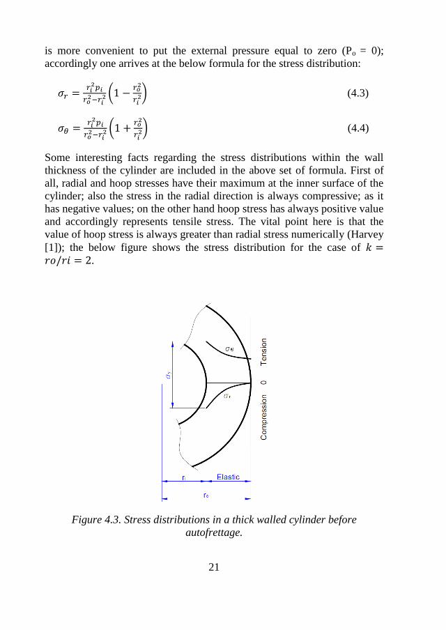
Some interesting facts regarding the stress distributions within the wall
thickness of the cylinder are included in the above set of formula. First of
all, radial and hoop stresses have their maximum at the inner surface of the
cylinder; also the stress in the radial direction is always compressive; as it
has negative values; on the other hand hoop stress has always positive value
and accordingly represents tensile stress. The vital point here is that the
value of hoop stress is always greater than radial stress numerically (Harvey
[1]); the below figure shows the stress distribution for the case of .
Figure 4.3. Stress distributions in a thick walled cylinder before
autofrettage.
Page 24
22
4.2.2. Radial displacement before autofrettage
Radial displacement, u, at any point of the thick walled cylinder can be
derived as below (Boresi [5]):
(
)[( )(
)]
( )
( )
(4.5)
Where F is the axial force which can be calculated from the below relation
(Boresi [5]):
(
) (
) (4.6)
The value of radial displacement will be used as a quantity to check the
validity of the Abaqus preliminary model.
4.2.3. Stress components after autofrettage
Now that the stress components of a non-autofrettaged thick walled
cylinder have been derived, it is logical to examine the effect of
autofrettage on the stress components. Assuming the condition of elastic-
perfectly plastic material together with the Tresca yield criterion, below
relations are presented for the radial and hoop stress components after
autofrettage for a thick walled cylinder (Benham [2]):
(
) (4.7)
(
)
(
) (4.8)
Figure 4.3 shows the distribution of stress components after autofrettage
across the thickness of the thick walled cylinder. As it is obvious from the
figure, autofrettage is caused the maximum of the hoop stress component to
Page 25
23
relocate from the bore of the cylinder to somewhere inside the thickness of
the cylinder.
Figure 4.4. Stress distributions in a thick walled cylinder after autofrettage.
4.3. A brief introduction to plasticity
The pervious section illustrates the key role of plastic region in the
autofrettage process. Therefore, it is advantageous to provide a brief
introduction to this subject in this section. For a more comprehensive study,
the interested reader is referred to (Ottosen et al. [12]).
Plasticity can be referred as the material behaviour beyond its yield point
where the structure or body does not recover to its initial shape when
unloaded (Ottosen et al. [12]). The below figure illustrates the general stress
strain relation beyond the yield point obtained from a simple tensile test in
order to provide a better understanding of the concept.
Page 26
24
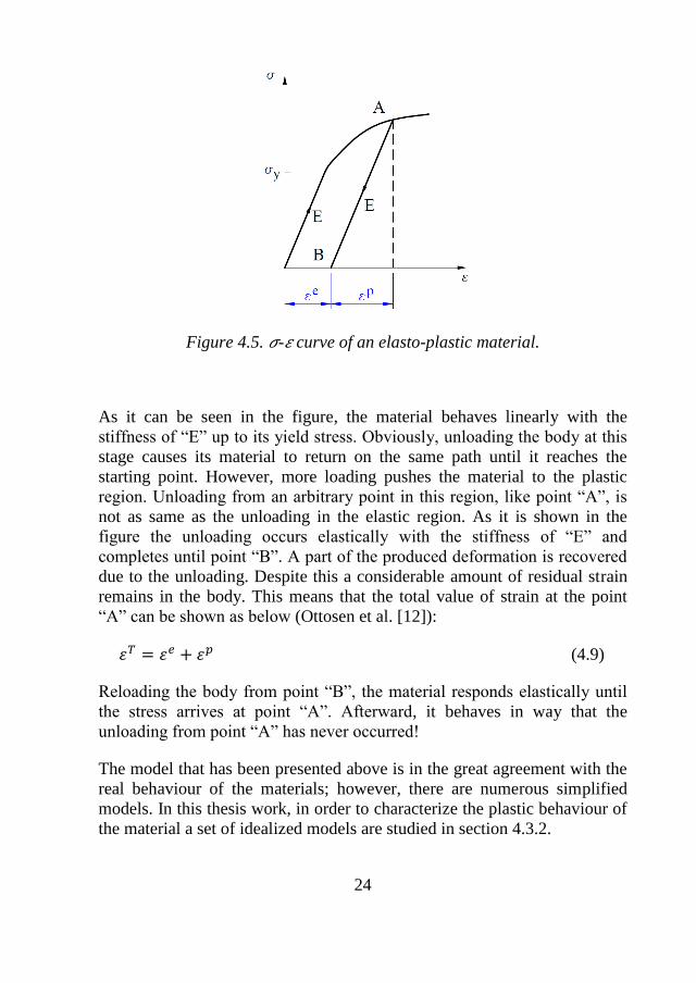
Figure 4.5. -𝜀 curve of an elasto-plastic material.
As it can be seen in the figure, the material behaves linearly with the
stiffness of “E” up to its yield stress. Obviously, unloading the body at this
stage causes its material to return on the same path until it reaches the
starting point. However, more loading pushes the material to the plastic
region. Unloading from an arbitrary point in this region, like point “A”, is
not as same as the unloading in the elastic region. As it is shown in the
figure the unloading occurs elastically with the stiffness of “E” and
completes until point “B”. A part of the produced deformation is recovered
due to the unloading. Despite this a considerable amount of residual strain
remains in the body. This means that the total value of strain at the point
“A” can be shown as below (Ottosen et al. [12]):
𝜀 𝜀 𝜀 (4.9)
Reloading the body from point “B”, the material responds elastically until
the stress arrives at point “A”. Afterward, it behaves in way that the
unloading from point “A” has never occurred!
The model that has been presented above is in the great agreement with the
real behaviour of the materials; however, there are numerous simplified
models. In this thesis work, in order to characterize the plastic behaviour of
the material a set of idealized models are studied in section 4.3.2.
Page 27
25
4.3.1. Yield criteria and yield surfaces
Yield criteria are design tools that can be utilized to predict the value of
stress that should be achieved in order for a solid body to undergo plastic
deformation in the condition of complex stress. Although there are different
yield criteria, in this project two of the most famous ones namely, von
Mises and Tresca criteria are used. It is worthy to note that, these theories
of yielding are mostly expressed in terms of principal stresses.
According to the von Mises criterion the value of the stress that brings the
material into the plastic region, should fulfill the below equation (Bower
[13]).
( 𝜀 ) √
[( ) ( ) ( ) ] (𝜀
)
(4.10)
For the case of Tresca criterion the below relation holds (Bower [13]).
( 𝜀 ) {| | | | | |} (𝜀
)
(4.11)
Where, σij represents general stress state in the solid and σ1,σ2 and σ3 are
the principal stresses. Also, “Y” represents the yield stress which is a
function of total plastic strain of the solid (Bower [13]).
Yield surface is used as a graphical way of presenting an arbitrary state of
stress in the “principal stress space”. Principal stress space is a coordinate
system which principal stresses are the axes of the coordinate system. In
this fashion, von Mises criterion can be presented as a cylinder with the
radius of r = Y/√3, as below (Bower [13]).
If the state of stress locates with in the cylinder the material behaves
elastically, in contrast to this, if it positions on the surface, the material
reaches its yield. Note that the space outside the cylinder is considered as
inaccessible.
Page 28
26
Figure 4.6. Von Mises yield surface.
A more convenient way of presenting yield surface is to view it in the
direction of the axis of the cylinder (Bower [13]). Axial view of the yield
surface for the case of von Mises and Tresca yield criterion are shown
below.
Figure 4.7. Axial view of von Mises and Tresca yield surfaces.
Page 29
27
These graphs show the locus of the yield points in the principal stress
space.
4.3.2. Bauschinger effect
Although, regardless of the sign, most of the common metals tend to have
the same value of yield stress for the both tension and compression
conditions, this is just for a narrow case of simple tensile or compression
tests on a virgin specimen.
Based on the sagacious discovery of J. Bauschinger in 1881, the value of
compression yield stress of a specimen decreases after being subjected to a
tensile load bigger than its tensile yield stress (Lemoin [14]). Practically,
this phenomenon might observe as a result of either simple cyclic loading
or revers loading of a virgin specimen. This phenomenon is called
Bauschinger effect after the name of its explorer.
4.3.3. Models of plasticity
As mentioned above in this thesis project two models for plasticity are
used, namely elastic-perfectly plastic and elastic-linear plastic. These two
models are further discussed here.
1- Elastic-perfectly plastic model
In order to consider the plastic behaviour of a material, the simplest
possible model is elastic-perfectly plastic. The behaviour of the model can
be illustrated as below (Ottosen [12]).
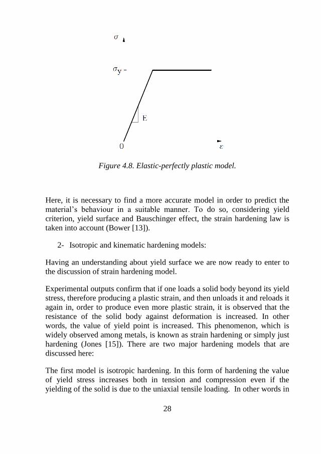
According to figure 4.8 once the material reaches its yield stress it
undergoes relatively huge amount of deformation. Note that in this model
the value of yield stress does not change due to the plastic strain (Ottosen
[12]). The only benefit of this model is its simplicity and, obviously, it is
not recommended to use the model for the case of complex analysis.
Page 30
28
Figure 4.8. Elastic-perfectly plastic model.
Here, it is necessary to find a more accurate model in order to predict the
material’s behaviour in a suitable manner. To do so, considering yield
criterion, yield surface and Bauschinger effect, the strain hardening law is
taken into account (Bower [13]).
2- Isotropic and kinematic hardening models:
Having an understanding about yield surface we are now ready to enter to
the discussion of strain hardening model.
Experimental outputs confirm that if one loads a solid body beyond its yield
stress, therefore producing a plastic strain, and then unloads it and reloads it
again in, order to produce even more plastic strain, it is observed that the
resistance of the solid body against deformation is increased. In other
words, the value of yield point is increased. This phenomenon, which is
widely observed among metals, is known as strain hardening or simply just
hardening (Jones [15]). There are two major hardening models that are
discussed here:
The first model is isotropic hardening. In this form of hardening the value
of yield stress increases both in tension and compression even if the
yielding of the solid is due to the uniaxial tensile loading. In other words in
Page 31
29
this kind of hardening the initial yield surface of the material expands
almost uniformly, while the centre and the shape of the yield surface
remains untouched (Jones [15]).
Based on what has been already explained regarding the Bauschinger
effect, it can be easily found out that this effect is not included in isotropic
hardening (Jones [15]). This is illustrated in the below figure.
Figure 4.9. Isotropic hardening model.
In contrast to the isotropic hardening another model of hardening exists
which includes the Bauschinger effect namely, kinematic hardening. This
model suggests that the yield surface keeps its shape while have a
translation movement just like a rigid body (Jones [15]). A schematic below
figure shows the kinematic hardening effect on a yield surface:
The critical point to remember here is that the kinematic hardening model is
suitable for describing the behaviour of metals under the condition of cyclic
loading.
Page 32
30
Figure 4.10. Kinematic hardening model.
4.4. Source of nonlinearity in this study
A very important issue that is needed to be addressed in the procedure of
analyzing any mechanical engineering problem using a FEM computer
suite is the linear or nonlinear behaviour of the system to be studied.
Although nearly all of the real world problems have a level of nonlinearity,
in the most cases it is possible to treat the problem linearly. This should be
done by providing logical assumption(s).
In the field of solid mechanics the sources of nonlinearity can be
categorized into three different groups as follows [19]
Material nonlinearity
Geometric nonlinearity
Boundary nonlinearity
The first source of nonlinearity happens when due to a set of reasons a
nonlinear relationship rules the stress-strain correlation in the problem.
While the second sources of nonlinearity take places when a change in the
geometry of the problem results in a considerable change in the load-
deformation behaviour of the problem (Bonet et al. [16]). Finally, the third
Page 33
31
case is a result of a change in the boundary conditions. Contact is a
common phenomenon accompanied with this form of nonlinearity.
As it has already been discussed, the procedure of autofrettage is not
accompanied by considerable changes in the dimensions of the solid bodies
while it establishes a plastic region in the solid body which is the most
common case of material nonlinearity. Accordingly, it is obvious that
autofrettage should be considered as a process with material nonlinearity.
Page 34
32
5. Autofrettage in Abaqus
Abaqus is a finite element analysis computer software suite which is
capable of solving a wide range of problems from different areas of
mechanical engineering such as solid mechanics, fluid mechanics, heat
transfer and vibration problems. This suite is equipped with three core
software, namely, Abaqus/CAE, Abaqus/standard and Abaqus/explicit.
Abaqus/CAE refers to the Abaqus environment and its modelling and
visualization equipment. It provides user with the CAD tools, assembly and
meshing options at the pre-processing stage beside result visualization at
the post processing level.
Abaqus/standard is responsible for solving the traditional mechanical
engineering problems such as static, dynamic and thermal problems. It has
the ability to solve both linear and nonlinear problems. On the other hand,
Abaqus/explicit is used for more complex cases of transient dynamics and
quasi-static problems. It is usually used to solve the problem with a very
high level of nonlinearity [15].
Figure 5.1. Abaqus modules.
Page 35
33
As it can be seen in the figure 5.1 in order to solve a problem in Abaqus
one should go through a set of different sections known as Abaqus’
modules, namely, Part, Property, Assembly, Step, Interaction, Load, Mesh,
Optimization, Job, Visualization and Sketch. Certainly, if each module is
defined correctly, it is more likely to obtain a reliable study.
In the procedure of this thesis, modules of property, in order to properly
define the plasticity, and load, for the correct applying of cyclic loading and
boundary conditions are more important.
To analyse the effect of autofrettage process on the valve house, this part,
because of its shape and geometry, needs to be modelled three
dimensionally in Abaqus. As it has already been mentioned because of the
more typical geometry of the pipe and for the validity of the obtained
results from the study of the valve house, first the autofrettage analysis of
the 3D model of the pipe is verified in Abaqus, as a stepping stone. Then
the same approach, considering boundary conditions, material properties,
element type, etc., is used for the valve house.
5.1. Autofrettage analysis of the pipe
In this section the following steps are followed:
Verification of the pipe model; considering an elastic material, the
pipe model is subjected to a relatively low pressure in Abaqus and
using the analytical relations the validity of the simulation is
checked and a suitable model is chosen for the next step.
Autofrettage of the pipe; in this step, considering an elastic-plastic
material, the autofrettage procedure is adopted for the chosen model
and different angles of this process are studied.
Results of autofrettage of the pipe; finally, applying various
autofrettage and working pressures, different aspects of autofrettage
procedure are investigated.
Page 36
34
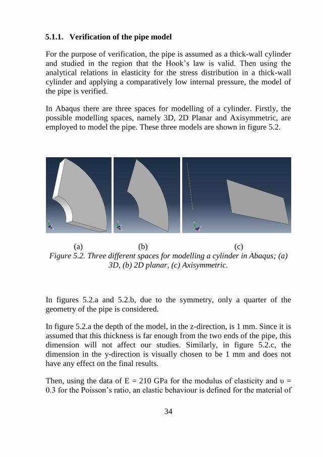
5.1.1. Verification of the pipe model
For the purpose of verification, the pipe is assumed as a thick-wall cylinder
and studied in the region that the Hook’s law is valid. Then using the
analytical relations in elasticity for the stress distribution in a thick-wall
cylinder and applying a comparatively low internal pressure, the model of
the pipe is verified.
In Abaqus there are three spaces for modelling of a cylinder. Firstly, the
possible modelling spaces, namely 3D, 2D Planar and Axisymmetric, are
employed to model the pipe. These three models are shown in figure 5.2.
(a) (b) (c)
Figure 5.2. Three different spaces for modelling a cylinder in Abaqus; (a)
3D, (b) 2D planar, (c) Axisymmetric.
In figures 5.2.a and 5.2.b, due to the symmetry, only a quarter of the
geometry of the pipe is considered.
In figure 5.2.a the depth of the model, in the z-direction, is 1 mm. Since it is
assumed that this thickness is far enough from the two ends of the pipe, this
dimension will not affect our studies. Similarly, in figure 5.2.c, the
dimension in the y-direction is visually chosen to be 1 mm and does not
have any effect on the final results.
Then, using the data of E = 210 GPa for the modulus of elasticity and υ =
0.3 for the Poisson’s ratio, an elastic behaviour is defined for the material of
Page 37
35
the pipe. This material is assigned to the section and the part is then
assembled. Afterwards, for each modelling space the following sets of
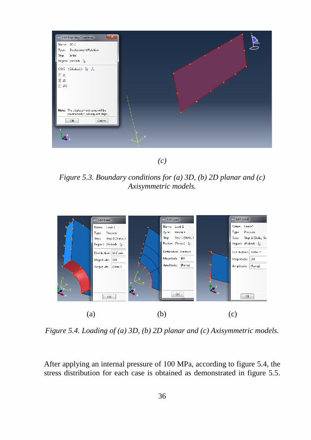
boundary conditions are defined as shown in figure 5. 3.
(a)
(b)
Page 38
36
(c)
Figure 5.3. Boundary conditions for (a) 3D, (b) 2D planar and (c)
Axisymmetric models.
(a) (b) (c)
Figure 5.4. Loading of (a) 3D, (b) 2D planar and (c) Axisymmetric models.
After applying an internal pressure of 100 MPa, according to figure 5.4, the
stress distribution for each case is obtained as demonstrated in figure 5.5.
Page 39
37
As it is obvious from the figure below, the three models provide a very
close results of avarage of von Mises stress distributions.
Figure 5.5. Stress distribution for three studied cases.
It is to mention that the above stress values have been extracted from the
radial direction as shown in the figure 5.6.
Although according to figure 5.5, all the above studies end to the same
results, based on the calculation time and the definition of the problem, the
axisymmetric model is preferred here for autofrettage analysis.
Page 40
38
(a) (b) (c)
Figure 5.6. Stress distribution for three studied cases.
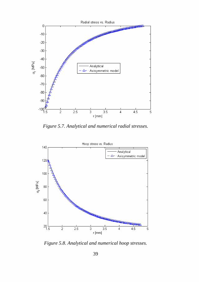
The axisymmetric result is compared with the analytical results obtained
from relations 4.1 and 4.2 for the radial and circumferential stresses in a
thick-wall cylinder. Considering Pi = 100 MPa, Po = 0, a = 1.5 mm and b =
4.75 mm, these relations for this work will be as follows.
( ) (5.1)
( ) (5.2)
From the above relations it is evident that the prevailing component of the
stress is in the hoop direction. The below figures show the analytical
outputs of radial stress, hoop stress and displacement together with the
numerical results of the axisymmetric study obtained from Abaqus.
Page 41
39
Figure 5.7. Analytical and numerical radial stresses.
Figure 5.8. Analytical and numerical hoop stresses.
Page 42
40
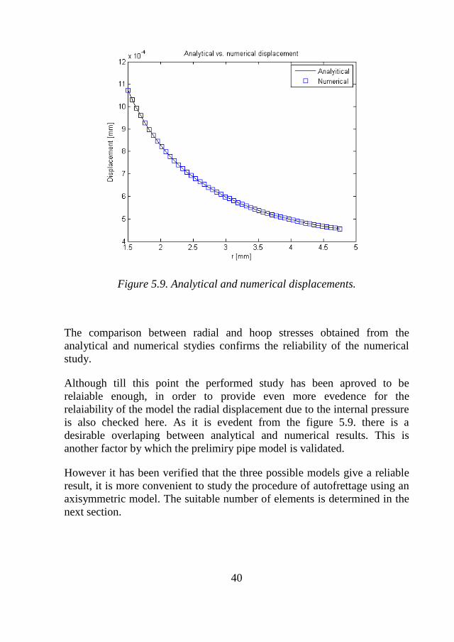
Figure 5.9. Analytical and numerical displacements.
The comparison between radial and hoop stresses obtained from the
analytical and numerical stydies confirms the reliability of the numerical
study.
Although till this point the performed study has been aproved to be
relaiable enough, in order to provide even more evedence for the
relaiability of the model the radial displacement due to the internal pressure
is also checked here. As it is evedent from the figure 5.9. there is a
desirable overlaping between analytical and numerical results. This is
another factor by which the prelimiry pipe model is validated.
However it has been verified that the three possible models give a reliable
result, it is more convenient to study the procedure of autofrettage using an
axisymmetric model. The suitable number of elements is determined in the
next section.
Page 43
41
5.1.2. Autofrettage of the pipe
As mentioned before, the effect of autofrettage is firstly studied using an
axisymmetric model. To do so, the appropriate number of elements is
determined considering the convergence in the von Mises stress. Since
during the autofrettage procedure the location of the maximum stress
varies, all the nodal values along the radius have the same importance and
are considered. Therefore, the area under the average von Mises stress
curve is taken into account for this purpose.
Figure 5.10 illustrates that with 100 elements along r-direction the area
under the von Mises stress is acceptably convergent. It is also to be noted
that for this study, due to the change in location of the maximum stress,
using bias in meshing is not suitable. Therefore, considering the same
boundary condition as before in figure 5.3.c, the model of the pipe is
meshed according to figure 5.11.
Figure 5.10. Convergence of element numbers.
Page 44
42
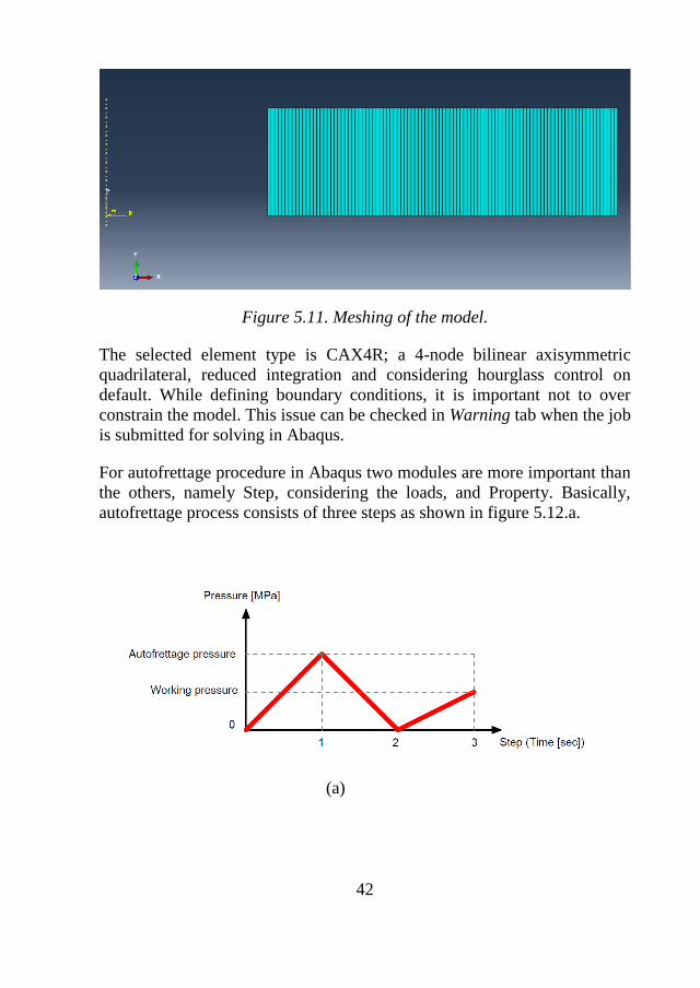
Figure 5.11. Meshing of the model.
The selected element type is CAX4R; a 4-node bilinear axisymmetric
quadrilateral, reduced integration and considering hourglass control on
default. While defining boundary conditions, it is important not to over
constrain the model. This issue can be checked in Warning tab when the job
is submitted for solving in Abaqus.
For autofrettage procedure in Abaqus two modules are more important than
the others, namely Step, considering the loads, and Property. Basically,
autofrettage process consists of three steps as shown in figure 5.12.a.
(a)
Page 45
43
(b)
Figure 5.12. Two different ways of applying pressure based on the concept
of step in Abaqus.
In step 1 the pipe is subjected to the autofrettage pressure and then released
in step 2. In the third step the pipe is reloaded under the effect of the
autofrettage as shown in the figure 5.12.a. In Abaqus, according to default
of the program and in order to save the computing time, the second step can
be omitted and the results remain the same as in figure 5.12.b. Here, in the
Step Module, the steps are General Static with the length of 1 second;
however time does not have a physical quantity meaning in this study.
Another significant module in Abaqus, as the core area of the autofrettage
study, is Property. In this module elastic-plastic behaviour of the material is
defined. The material that is used in this work has an engineering stress-
strain curve, based on a tensile test, according to figure 5.13.
Page 46
44
Figure 5.13. Nominal(engineering) stress-strain diagram.
In order to define plasticity in Abaqus, these nominal stress-strain values
must be converted to true stress-strain values using the following relations
(Johnson et al. [17]).
𝜀 ( 𝜀 ) (5.3)
( 𝜀 ) (5.4)
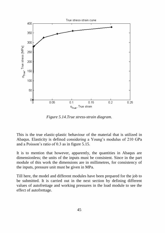
This transformation results in the true stress-strain curve of the material as
shown in figure 5.14.
Page 47
45
Figure 5.14.True stress-strain diagram.
This is the true elastic-plastic behaviour of the material that is utilized in
Abaqus. Elasticity is defined considering a Young’s modulus of 210 GPa
and a Poisson’s ratio of 0.3 as in figure 5.15.
It is to mention that however, apparently, the quantities in Abaqus are
dimensionless; the units of the inputs must be consistent. Since in the part
module of this work the dimensions are in millimetres, for consistency of
the inputs, pressure unit must be given in MPa.
Till here, the model and different modules have been prepared for the job to
be submitted. It is carried out in the next section by defining different
values of autofrettage and working pressures in the load module to see the
effect of autofrettage.
Page 48
46
Figure 5.15. Defining elasticity.
As illustrated in figure A.12, each strain quantity in the true stress-strain
diagram consists of two elastic and plastic regions. In order for defining the
plastic behaviour of the material in Abaqus, these total strains must be
decomposed into the elastic and plastic components using the following
relation
𝜀 𝜀 𝜀 (5.5)
in which εe, εP
and εT are elastic strain, plastic strain and total strain,
respectively.
Page 49
47
Figure 5.16. The relation of elastic, plastic and total strain.
Figure 5.17. Defining plasticity.
Page 50
48
The converted data are then used for plasticity definition in Abaqus,
according to figure 5.17.
In order to provide a more accurate autofrettage analysis of the pipe, the
Bauschinger effect is also modelled with the nonlinear isotropic/kinematic,
or combined, hardening. This prediction, choosing a data type of Half
Cycle, is highlighted above.
So far, the model and the modules have been well prepared and the job can
be submitted. In the next section, different autofrettage and working
pressures are applied to the pipe and different aspects of autofrettage are
studied and discussed.
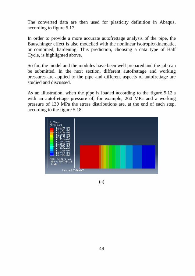
As an illustration, when the pipe is loaded according to the figure 5.12.a
with an autofrettage pressure of, for example, 260 MPa and a working
pressure of 130 MPa the stress distributions are, at the end of each step,
according to the figure 5.18.
(a)
Page 51
49
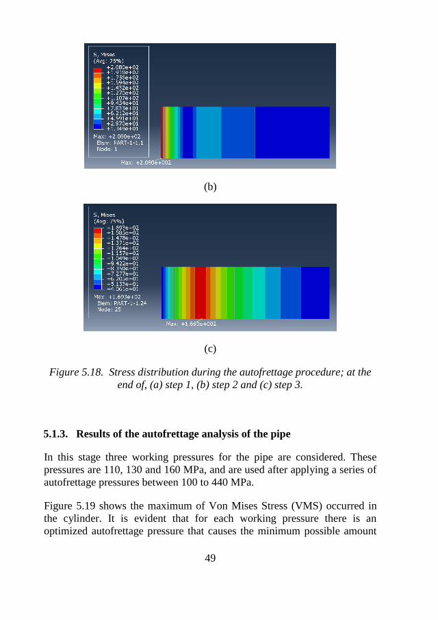
(b)
(c)
Figure 5.18. Stress distribution during the autofrettage procedure; at the
end of, (a) step 1, (b) step 2 and (c) step 3.
5.1.3. Results of the autofrettage analysis of the pipe
In this stage three working pressures for the pipe are considered. These
pressures are 110, 130 and 160 MPa, and are used after applying a series of
autofrettage pressures between 100 to 440 MPa.
Figure 5.19 shows the maximum of Von Mises Stress (VMS) occurred in
the cylinder. It is evident that for each working pressure there is an
optimized autofrettage pressure that causes the minimum possible amount
Page 52
50
of VMS. For example, if the working pressure is 160 MPa, an autofrettage
pressure of 280 MPa gives the minimum possible of VMS.
Figure 5.19. Maximum of VMS in different studies.
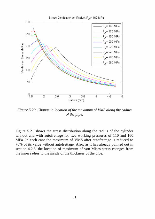
The stress distribution along the radius of the cylinder is illustrated in figure
5.20 for different autofrettage pressures, from 160 to 280 MPa, and a
working pressure of only 160 MPa. In this figure the change in the location
of maximum stress is obvious.
Page 53
51
Figure 5.20. Change in location of the maximum of VMS along the radius
of the pipe.
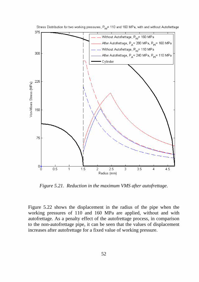
Figure 5.21 shows the stress distribution along the radius of the cylinder
without and with autofrettage for two working pressures of 110 and 160
MPa. In each case the maximum of VMS after autofrettage is reduced to
70% of its value without autofrettage. Also, as it has already pointed out in
section 4.2.3, the location of maximum of von Mises stress changes from
the inner radius to the inside of the thickness of the pipe.
Page 54
52
Figure 5.21. Reduction in the maximum VMS after autofrettage.
Figure 5.22 shows the displacement in the radius of the pipe when the
working pressures of 110 and 160 MPa are applied, without and with
autofrettage. As a penalty effect of the autofrettage process, in comparison
to the non-autofrettage pipe, it can be seen that the values of displacement
increases after autofrettage for a fixed value of working pressure.
Page 55
53
Figure 5.22. Displacement in r-direction.
5.1.3.1 Minimum and maximum of the autofrettage pressure
The minimum of autofrettage pressure, Py1, is the pressure at which the
inner radius of the cylinder, r = a, starts yielding. While at Py2 the outer
surface, r = b, yields. According to Xiaoying and Gnagling [18] and based
on von Mises yield criteria, these two pressures are determined as follows.
√ (5.6)
Page 56
54
√ |
(
)
( )|
( )( )⁄
[√ ( )
(
)]
(5.7)
in which σy is the yield stress and k is the ratio of outside to inside radius, k
= b/a.
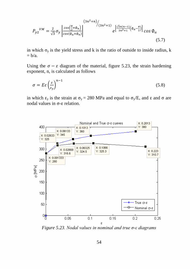
Using the 𝜀 diagram of the material, figure 5.23, the strain hardening
exponent, n, is calculated as follows
𝜀 (
)
(5.8)
in which εy is the strain at σy = 280 MPa and equal to σy/E, and ε and σ are
nodal values in σ-ε relation.
Figure 5.23. Nodal values in nominal and true σ-ε diagrams
Page 57
55
It implies that
(
)(
)
(5.9)
Having n, auxiliary variables of n and a, are determined as follows
√
√ (5.10)
√
(
) |
(
)
( )|
( )⁄
[√ ( )
(
)]
(5.11)
Considering n = 0.059, and using a proper MATLAB code, we arrive at n
= 0.4676π and a= 0.1087π.
Substituting the above values in relations (5.6) and (5.7) leads to the
minimum and maximum of autofrettage pressures based on the von Mises
yield criteria.
Py1VM
= 145.3 MPa
Py2 VM
= 377.9 MPa
Another analytical approach to determine the minimum and maximum of
the autofrettage pressures is using Tresca yield criteria (Xiaoying et al.
[18]).
√ ( ) (5.12)
( )
⁄
(5.13)
in which k is the ratio of outer to inner radius and A = 1 and B = √3 are
constant. These relations result in the minimum and maximum of
autofrettage pressures based on the Tresca yield criteria.
Page 58
56
Py1T
= 143.3 MPa
Py2 T
= 218 MPa
The two above sets of obtained pressures are then compared to the
numerical results from Abaqus analysis. It is predictable that the von Mises
yield criteria give more accurate results since the plastic behaviour of the
material, using σ-ε diagram, is taken into account.
5.24. Minimum and maximum of the autofrettage pressure.
According to figure 5.24, the minimum and maximum of autofrettage
pressure are
Py1Num
= 140 MPa
Page 59
57
Py2 Num
= 390 MPa
In this study the working pressure is set to be 130 MPa and autofrettage
pressures vary from 100 to 440 MPa.
If it is considered that the under study thick-wall cylinder fails when its
outer surface yields, Py2 can be also called burst pressure [Majzoobi et al.].
This failure might be occurred due to, for example, a crack initiation in the
outer surface of the pipe. However in order to check the validity of the
bursting pressures a practical experiment should be performed. Table 5.1
concludes the achieved minimum and maximum of autofrettage pressures
using different approaches.
Table 5.1. Minimum and maximum of autofrettage pressure.
Approach
Pressure
Tresca yield
criteria
von Mises
yield criteria
Numerical
analysis
Min. of autofrettage
pressure [MPa] 143.3 145.3 140
Max. of autofrettage
pressure (Bursting
pressure) [MPa]
218 377.9 390
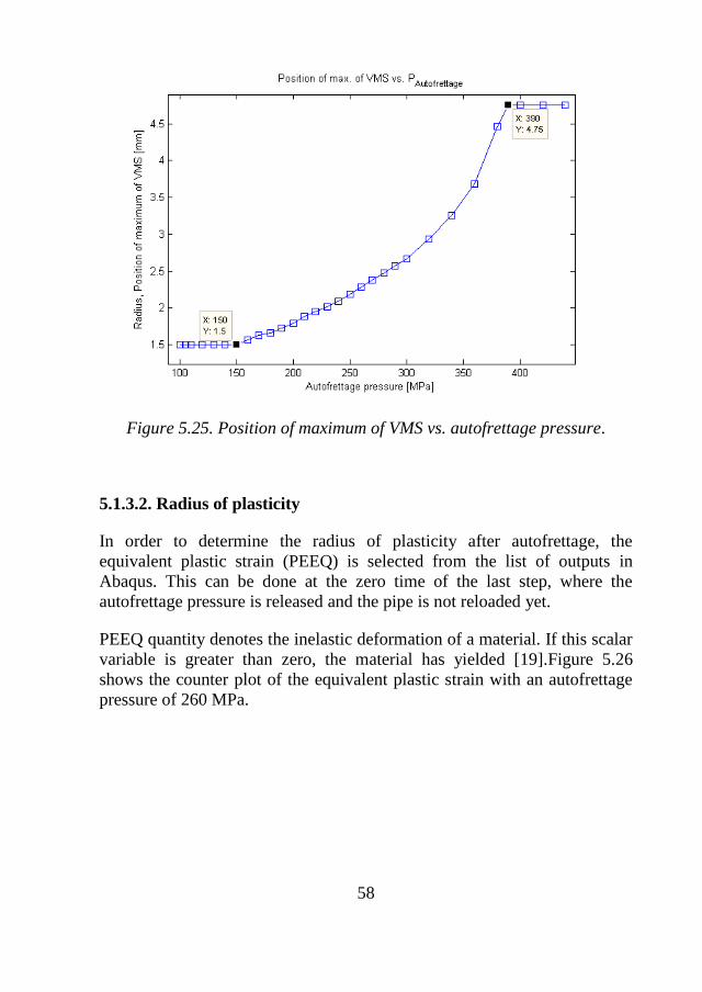
Figure 5.25 shows the position of maximum of von Mises stress when the
working pressure is 130 MPa and for different autofrettage pressures.
Page 60
58
Figure 5.25. Position of maximum of VMS vs. autofrettage pressure.
5.1.3.2. Radius of plasticity
In order to determine the radius of plasticity after autofrettage, the
equivalent plastic strain (PEEQ) is selected from the list of outputs in
Abaqus. This can be done at the zero time of the last step, where the
autofrettage pressure is released and the pipe is not reloaded yet.
PEEQ quantity denotes the inelastic deformation of a material. If this scalar
variable is greater than zero, the material has yielded [19].Figure 5.26
shows the counter plot of the equivalent plastic strain with an autofrettage
pressure of 260 MPa.
Page 61
59
Figure 5.26. Contour of equivalent plastic strain (PEEQ).
It is obvious from the figure that the maximum plastic strain in the counter
legend is about 0.2%. After the minimum value of zero, at node 26, the
material has still an elastic behaviour. In this step, in order to have a more
accurate result, using the query tool in Abaqus, the minimum value of
PEEQ is checked at the integration points and the radius of plasticity is
calculated. Figure 5.27 shows the location of minimum and maximum
value of PEEQ.
Figure 5.27. PEEQ at integration points.
Page 62
60
PEEQ is zero at integration point of element 25 that includes node 26. This
node has an original coordinates of (2.3125, 0, 0), before deformation, that
results in a radius of 2.3125 mm. Therefore, the effect of autofrettage on the
material behaviour in the pipe is illustrated in figure 5.28 in which two
elastic and plastic regions are depicted.
Figure 5.28. Elastic and plastic regions without considering displacement
due to the autofrettage.
However, after deformation and considering the occurred strains, the pipe
has the following real dimensions.
Figure 5.29. Elastic and plastic regions considering displacement due to
the autofrettage.
Page 63
61
Figure 5.30 shows the PEEQ diagram for different autofrettage pressures.
In order for investigation of radius of plasticity the working pressure is not
taken into account. This is also the case for study of residual stresses where
the data are gathered when the autofrettage pressure is released and the pipe
is not reloaded yet.
The blue curve, in figure 5.30, belongs to the autofrettage pressure of 260
MPa on which the radius of plasticity is specified. This is in agreement with
the calculated and shown value in the figure 5.29.
Figure 5.30. PEEQ diagram for different autofrettage pressures.
Page 64
62
5.1.3.3. Residual stresses
Residual stresses are determined for the same case as in previous section,
for an autofrettage pressure of 260 MPa. First, let’s assume a condition in
which the pipe is not autofrettaged and is subjected to a working pressure of
130 MPa directly. In this case the von Mises stress and its stress
components are as shown in figure 5.30.
It is obvious from the below figure that at the radius of r = 2.377 mm the
stress components have the value of
These principal stress components result in the von Mises yield criterion as
follows
√
[( )
( ) ( )
] (5.14)
This results in σVM = 99.74 MPa that is equal to the specified value on the
black curve in figure 5.31.
Page 65
63
Figure 5.31. Stress components without autofrettage, PWorking = 130 MPa.
The same manner is used for the investigation of residual stresses after the
autofrettage process. Figure 5.32 shows the residual stress components, and
their corresponding values at r = 2.377, when the autofrettage pressure of
260 MPa is applied to the pipe and then released.
Page 66
64
Figure 5.32. Stress components after autofrettage, PAutofrettage = 260 MPa.
Figure 5.33. Von Mises stress, its components, and residual stresses.
Page 67
65
In figure 5.33, these residual stresses after autofrettage are compared with
the stress components for the case that no autofrettage pressure is taken into
account and the pipe is applied to the working pressure of 130 MPa
directly.
Zooming into the above figure, the different stress values are determined at,
for example, r = 2.377 mm as follows.
Figure 5.34. Stress values at r = 2.377 mm.
In order to investigate the effect of autofrettage process the above study
leads to the following set of data, as shown in table 5.2.
Accordingly, it is shown that, after the autofrettage procedure, the von
Mises stress is obtained by superposition of the two above residual stresses
and stress components.
Page 68
66
[
[((
) (
))
((
)
(
)) ((
) (
))
]]
⁄
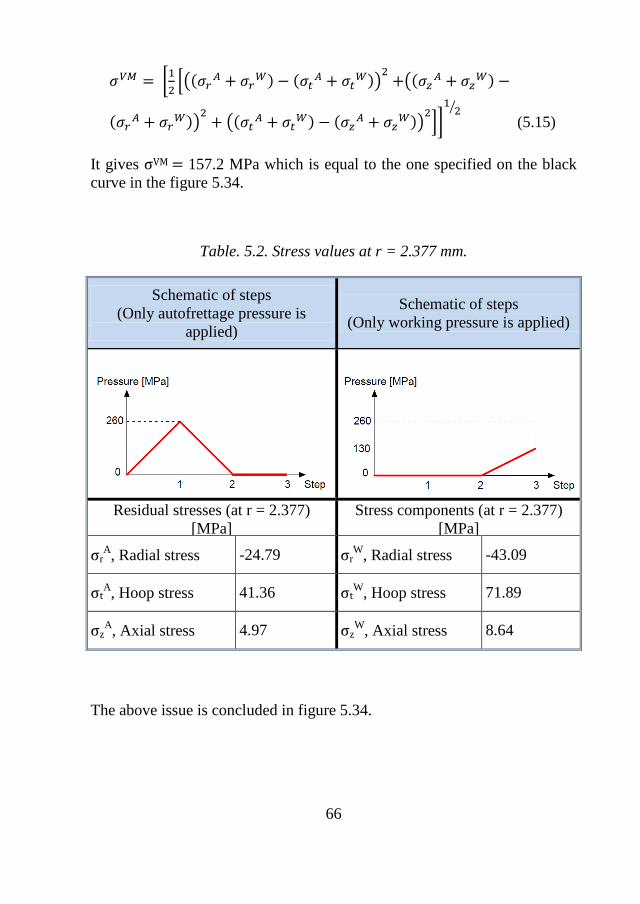
(5.15)
It gives σVM = 157.2 MPa which is equal to the one specified on the black
curve in the figure 5.34.
Table. 5.2. Stress values at r = 2.377 mm.
Schematic of steps
(Only autofrettage pressure is
applied)
Schematic of steps
(Only working pressure is applied)
Residual stresses (at r = 2.377)
[MPa]
Stress components (at r = 2.377)
[MPa]
σrA, Radial stress -24.79 σr
W, Radial stress -43.09
σtA, Hoop stress 41.36 σt
W, Hoop stress 71.89
σzA, Axial stress 4.97 σz
W, Axial stress 8.64
The above issue is concluded in figure 5.34.
Page 69
67
Figure 5.35. The combination of results of two studies in left-hand side, is
equal to the result of a three- step study in the right –hand side.
It can be concluded from the above study that the value of total stress is the
sum of residual stress, after autofrettage, and stress components, without
autofrettage procedure.
5.2. Autofrettage analysis of the valve house
In this section the following steps are followed:
Preparing a 3D study; in the first step, a 3D model of the pipe is
analysed and the results are compared to the results of the
axisymmetric model from the previous subchapter. Then by a
change in the geometry, this new model is turned into the analysis
of the valve house.
Autofrettage of the valve house; in this step, assuming a suitable
elastic-plastic material, the autofrettage procedure is simulated.
Results of autofrettage of the pipe; in the end, applying a set of
autofrettage and working pressures, different aspects of autofrettage
procedure are shown.
5.2.1. Preparing a 3D study
Figure 5.36 shows a 3D model of half of the pipe in which the length of the
pipe is selected to be 0.0325 mm. Half of the pipe is considered, rather than
a quarter or a sector of it, because in further studies the most simplified
Page 70
68
model of the valve house could be a half cut. In order to have the same
number of elements as in axisymmetric study, edges of the model in r-
direction are divided into 100 seeds. Therefore, in r-direction, length of
each division will be 0.0325 mm. If the number of elements in z-direction is
going to be 1, for the sake of simplicity, then the thickness of the pipe needs
to be 0.0325 mm, equal to the extruded length of the pipe.
Figure 5.36. 3D model of the pipe; number of elements in each direction.
1 element in
z-direction
100 elements in x- and y-
directions (or radial directions)
Page 71
69
Consequently, the meshed part will have the appearance as shown in the
figure 5.37. In this case, the element type of C3D4, a 4-node linear
tetrahedron, is employed. This element has a similar characteristic as the
one used in the axisymmetric study. This is also suitable for the further
analysis of the valve house.
Figure 5.37. Meshed 3D model; 1 element in z-direction and 100 elements
in x-direction are visible.
Figure 5.38 illustrates boundary conditions that are defined in the same
manner as in figure 5.3.a.
Page 72
70
Figure 5.38. Boundary conditions.
(a) (b)
Figure 5.39. Applying (a) autofrettage and (b) working pressures.
Loads are defined as shown in figure 5.39. In the first step, figure 5.38.a, an
autofrettage pressure of 260 MPa is applied. Then, in figure 5.38.b, without
a decreasing pressure, a working pressure of 130 MPa is applied in the
second step. The result of this analysis is compared with the one obtained
by the axisymmetric model in the previous sections. This comparison is
illustrated in figure 5.40.
Page 73
71
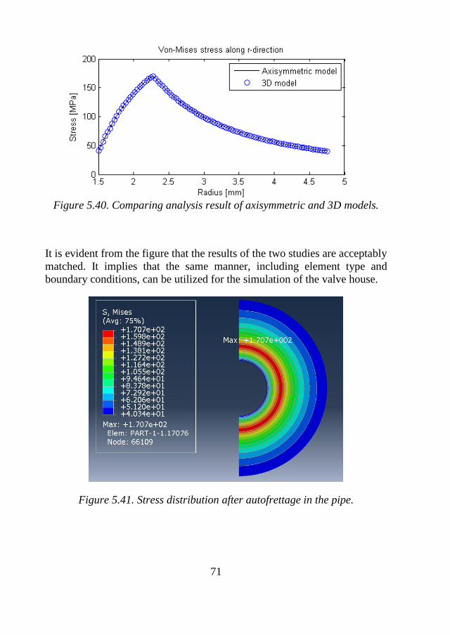
Figure 5.40. Comparing analysis result of axisymmetric and 3D models.
It is evident from the figure that the results of the two studies are acceptably
matched. It implies that the same manner, including element type and
boundary conditions, can be utilized for the simulation of the valve house.
Figure 5.41. Stress distribution after autofrettage in the pipe.
Page 74
72
5.2.2. Autofrettage of the valve house
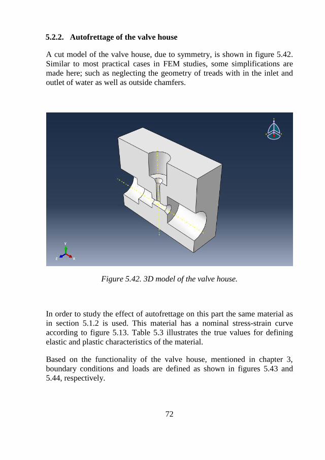
A cut model of the valve house, due to symmetry, is shown in figure 5.42.
Similar to most practical cases in FEM studies, some simplifications are
made here; such as neglecting the geometry of treads with in the inlet and
outlet of water as well as outside chamfers.
Figure 5.42. 3D model of the valve house.
In order to study the effect of autofrettage on this part the same material as
in section 5.1.2 is used. This material has a nominal stress-strain curve
according to figure 5.13. Table 5.3 illustrates the true values for defining
elastic and plastic characteristics of the material.
Based on the functionality of the valve house, mentioned in chapter 3,
boundary conditions and loads are defined as shown in figures 5.43 and
5.44, respectively.
Page 75
73
Table 5.3. Material property
Elasticity Plasticity
Modules of
elasticity (MPa) Poisson’s ratio
Stress
(MPa) Plastic strain
210e3 0.3
280 0
325 0.025
345 0.06
360 0.1
380 0.2
Figure 5.43. Assigned boundary conditions.
(a) (b)
Figure 5.44. Loads in steps 1 and 2; (a) applying autofrettage pressure and
(b) working pressure.
Page 76
74
In figure 5.44, as an illustration in the preliminary study, autofrettage
pressure is set to be 420 MPa and working pressure is 400 MPa.
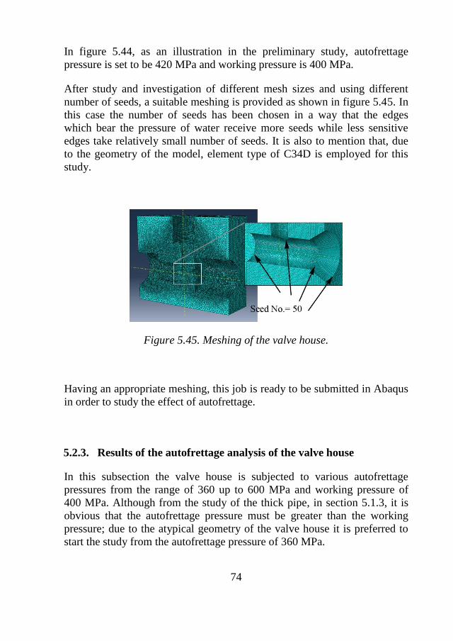
After study and investigation of different mesh sizes and using different
number of seeds, a suitable meshing is provided as shown in figure 5.45. In
this case the number of seeds has been chosen in a way that the edges
which bear the pressure of water receive more seeds while less sensitive
edges take relatively small number of seeds. It is also to mention that, due
to the geometry of the model, element type of C34D is employed for this
study.
Figure 5.45. Meshing of the valve house.
Having an appropriate meshing, this job is ready to be submitted in Abaqus
in order to study the effect of autofrettage.
5.2.3. Results of the autofrettage analysis of the valve house
In this subsection the valve house is subjected to various autofrettage
pressures from the range of 360 up to 600 MPa and working pressure of
400 MPa. Although from the study of the thick pipe, in section 5.1.3, it is
obvious that the autofrettage pressure must be greater than the working
pressure; due to the atypical geometry of the valve house it is preferred to
start the study from the autofrettage pressure of 360 MPa.
Page 77
75
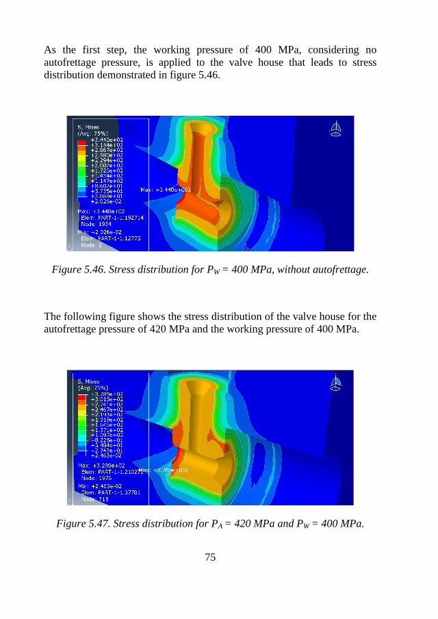
As the first step, the working pressure of 400 MPa, considering no
autofrettage pressure, is applied to the valve house that leads to stress
distribution demonstrated in figure 5.46.
Figure 5.46. Stress distribution for PW = 400 MPa, without autofrettage.
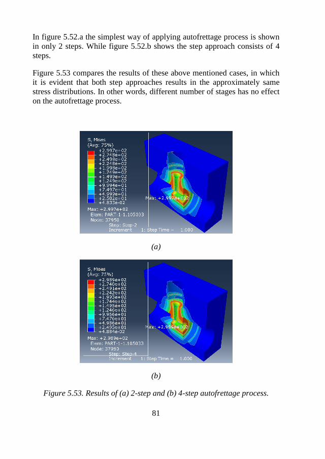
The following figure shows the stress distribution of the valve house for the
autofrettage pressure of 420 MPa and the working pressure of 400 MPa.
Figure 5.47. Stress distribution for PA = 420 MPa and PW = 400 MPa.
Page 78
76
It is obvious from the two above figures that after autofrettage the stress
distribution has reformed in a fashion that the regions of the valve house
which withstand the pressure undergo less stresses. As an example the
maximum value of VMS is decreased from 344 MPa to 328.9 MPa.
After going through a comprehensive study of autofrettage procedure, it is
timely to investigate the effect of different autofrettage pressures on the
valve house. As the main aim of this thesis work, it is of great interest to
obtain the optimized autofrettage pressure for the working pressure 400
MPa, this is the pressure in which the water jet cutting machine normally
works.
Figure 5.48. Maximum values of VMS for different autofrettage pressures.
Page 79
77
The graph shows that from the range of 400 to 540 MPa the autofrettage
process in effective. Also, it is obvious that the optimized value of
maximum VMS occurs at the autofrettage pressure of 480 MPa. In addition
to the above results, the location of maximum of VMS is also concluded in
the figure 5.49.
Figure 5.49. Zoomed location of maximum VMS.
Page 80
78
As another investigation in this subsection, PEEQ is utilized as a quantity in
order to illustrate the growth of plastic regime within the body of the valve
house. This is shown in figure 5.50 for the case of autofrettage pressure of
490 MPa.
Figure 5.50. Plastic region due to autofrettage pressure of 490 MPa.
As it is evidence form the above figure, the grey region has the PEEQ equal
to zero; this means that the region is still elastic.
5.2.3.1. Bigger working pressure, the same maximum VMS
According to figure 5.48, when the valve house is installed in the line,
having no autofrettage pressure, the component withstands a maximum
value of VMS equal to 344 MPa. Here it is of interest to find a bigger
working pressure that, after autofrettage, results in the same maximum
VMS.
For this purpose, the working pressure of, for example, 450 MPa is chosen.
Figure 5.51 shows the maximum values of VMS for different autofrettage
pressures 450 to 500 MPa.
Page 81
79
From this figure, it is obvious that using the autofrettage pressure of 480
MPa, the valve house bears the value of maximum VMS of 343.5 MPa,
approximately as in the case of working pressure of 400 MPa without any
autofrettage effects.
Figure 5.51. The maximum values of VMS for the working pressure of 450
MPa .
Since the working pressure leads to the velocity of water at the nozzle it has
the main role in the mechanism of water jet cutting technique. Accordingly,
this study is helpful to improve the efficiency of the system.
Page 82
80
5.2.3.2. Effect of different number of stages in autofrettage
As autofrettage itself is a simple procedure it is also convenient to perform
it in different steps. Here it is checked weather or not this leads to a more
efficient autofrettage results. The below graphs show two different step
approaches in order to apply autofrettage to the component of the valve
house. In this study the optimized autofrettage of 490 MPa for the case of
working pressure of 400 MPa is considered.
(a)
(b)
Figure 5.52. Two different step approaches to perform autofrettage.
Page 83
81
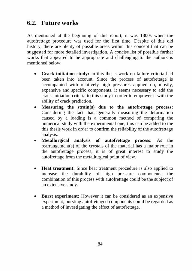
In figure 5.52.a the simplest way of applying autofrettage process is shown
in only 2 steps. While figure 5.52.b shows the step approach consists of 4
steps.
Figure 5.53 compares the results of these above mentioned cases, in which
it is evident that both step approaches results in the approximately same
stress distributions. In other words, different number of stages has no effect
on the autofrettage process.
(a)
(b)
Figure 5.53. Results of (a) 2-step and (b) 4-step autofrettage process.
Page 84
82
6. Conclusion and future works
6.1. Conclusion and discussion
Autofrettage is a procedure that is used to strength the structure of pressure
vessels by producing a plastic regime within their thickness. The aim of this
thesis work was to study the effect of autofrettage on two high pressure
components used in the water jet cutting machine, namely a conductor pipe
and the valve house of the cutting head assembly.
Because of the typical geometry of the conductor pipe as well as the
accessibility of the previous studies, as the initial study, the procedure of
autofrettage was modelled for the conductor pipe case. The pipe, as a thick
walled cylinder, was modelled asymmetrically. Afterward the obtained
model was verified using the analytical results of stress distribution
together with the deformation caused by the autofrettage process. Then as it
was needed to have a reliable 3D model, the approved axisymmetric model
was utilized to build a 3D one. The outputs of this 3D study were checked
using the axisymmetric part. Having an appropriate 3D model, the
autofrettage process of the valve house was the second stage of the study.
During the study of autofrettage in the pipe, the following results were
observed (see section 5.1.3)
The autofrettage pressure must be greater than the working pressure.
For each specific working pressure there is an optimized
autofrettage pressure.
This optimized autofrettage pressure reduces the value of maximum
Von Mises Stress (VMS). In this study, the reduction was
approximately 30%.
In addition to reduction in amount, the position of the maximum
VMS also relocate from the inner surface to the wall of the pipe.
The location of maximum VMS is on the boundary line of elastic
and plastic regions. This location is considered as the radius of
plasticity.
Residual stresses, and the residual hoop stresses above all, paly the
main role in the process of autofrettage.
Page 85
83
Autofrettage of the valve house was studied considering a working pressure
of 400 MPa and the following points were obtained.
The minimum and maximum of autofrettage pressures were
determined to be 400 and 540 MPa, respectively.
The optimized autofrettage pressure was 490 MPa.
The location of maximum VMS changed from the exterior edges,
subjected to pressure, to the thickness of the part.
The quantity of PEEQ was used to distinguish the plastic regime
after the autofrettage process.
The number of stages in applying a specific autofrettage pressure
did not have any effects on the results of the process.
In order for a reader to have a sense of the calculation time the below table,
lists the calculation time of some of the studied cases in this thesis work.
Table 6.1. Computation times.*
Part Pipe Valve house
Process Without autofrettage With autofrettage Without
autofrettage
With
autofrettage
Model 3D
2D
Ax
i.
3D
2D
Ax
i.
3D
3D
Element
type C3
D4
CP
E4
R
CA
X4
R
C3
D4
CP
E4
R
CA
X4
R
C3
D4
C3
D4
Element
No. 30
00
30
00
10
0
20
51
07
- 10
0
87
29
85
87
29
85
CPU time
hr:min:sec
00
:00:2
9
00
:00:2
3
00
:00:2
1
00
:07:2
7
-
00
:00:3
0
02
:39:2
8
03
:12:2
3
* All tables and figures are produced by the authors, except figure 1.1.
Page 86
84
6.2. Future works
As mentioned at the beginning of this report, it was 1800s when the
autofrettage procedure was used for the first time. Despite of this old
history, there are plenty of possible areas within this concept that can be
suggested for more detailed investigation. A concise list of possible further
works that appeared to be appropriate and challenging to the authors is
mentioned below:
Crack initiation study: In this thesis work no failure criteria had
been taken into account. Since the process of autofrettage is
accompanied with relatively high pressures applied on, mostly,
expensive and specific components, it seems necessary to add the
crack initiation criteria to this study in order to empower it with the
ability of crack prediction.
Measuring the strain(s) due to the autofrettage process: Considering the fact that, generally measuring the deformation
caused by a loading is a common method of comparing the
numerical study with the experimental one; this can be added to the
this thesis work in order to confirm the reliability of the autofrettage
analysis.
Metallurgical analysis of autofrettage process: As the
rearrangement(s) of the crystals of the material has a major role in
the autofrettage process, it is of great interest to study the
autofrettage from the metallurgical point of view.
Heat treatment: Since heat treatment procedure is also applied to
increase the durability of high pressure components, the
combination of this process with autofrettage could be the subject of
an extensive study.
Burst experiment: However it can be considered as an expensive
experiment, bursting autofrettaged components could be regarded as
a method of investigating the effect of autofrettage.
Page 87
85
7. References
1. Harvey, J. F., (1987), Theory and design of pressure vessels, CSB
Publishers & Distributors Pvt. Ltd.
2. Benham, P. P., Crawford, R. J. and Armstrong, C. G., (1996), Mechanics
of engineering materials, 2nd
edition, Longman Group Limited
3. Majzoobi, Gh. and Alavinia, A., (2006), Strength of materials, Vol.3, Bu-
Ali Sina University press
4. Gibson, M. C., (2008), Determination of residual stress distributions in
autofrettaged thick-walled cylinders, Ph.D. dissertation, Department of
engineering systems and management, Cranfield University, UK
5. Boresi, A. P., Schmidt, R. J. and Sidebottom, O. M., (1993), Advance
mechanics of materials, 5th
edition, John Wiley & sons Inc.
6. Perry, J. and Aboudi, J., (2003), Elasto-plastic stresses in thick walled
cylinders, ASME Journal of Pressure Vessel Technology, Vol.125, Issue 3.
7. Rees, D. W. A., (1990), Autofrettage theory and fatigue life of open-
ended cylinders, The Journal of Strain analysis for Engineering Design,
Vol.25, No.2.
8. White paper Autofrettage, Available from: http://www.maximator-
test.com/about/White-Paper-Autofrettage.pdf, Accessed: 21.05.2012.
9. Parker, A. P., (2001), Autofrettage of open end tubes-Pressures, Stresses,
Strains and code comparisons, ASME Journal of Pressure Vessel
Technology, Vol.123.
10. Huang, X. P., (2005), A general autofrettage model of a thick-walled
cylinder based on tensile-compressive stress-strain curve of a material,
Journal of Strain Analysis, Vol.40, No.6.
11. Hostford, W. F., (2005), Mechanical behavior of materials, Cambridge
University Press.
Page 88
86
12. Ottosen, N. S. and Ristinmaa, M., (2005), The mechanics of constitutive
modelling, Elsevier Ltd.
13. Bower, A. F., (2010), Applied Mechanics of Solids, CRC Press
14. Lemoine, X. and Aouafi, A., (2008), Bauschinger effect correspondence
of experimental tests, International Journal of material formatting, Vol.1,
Supplement 1.
15. Jones, R. M., (2009), Deformation theory of plasticity, Bull Ridge
Publishing.
16. Bonet, J. and Wood, R.D., (1997), Nonlinear continuum mechanics for
finite element analysis, Cambridge University Press.
17. Johnson, W. and Mellor, P. B., (1978), Engineering plasticity, Van
Nostrand Reinhold Inc.
18. Xiaoying, Z. and Gangling, L., (1984), In proceeding of the 5th
international conference on pressure vessel technology, Vol.1, ASME
united engineering centre.
19. Abaqus 6.10 documentation, (2010), Dassault Systems.
Page 89
87
Appendix
A. Stress distribution in a thick walled cylinder
The most general from of equations of equilibrium for a cylindrical volume
element in the radial, hoop and axial directions, as shown in figure 4.2, are
given in Boresi et al. [5] as follows.
(A.1)
(A.2)
(A.3)
Neglecting the effect of body forces (Boresi et al. [5]), the equation of
equilibrium for a cylindrical element can be reduced to below.
(A.4)
Beside this, the strain-displacement equations can be driven as below.
(A.5)
(A.6)
(A.7)
Also the stress-strain-temperature relations are
( ) (A.8)
Page 90
88
( ) (A.9)
( ) (A.10)
Note that α is the coefficient of linear thermal expansion. Substituting “u”
from A.6 into A.5 one gets
(A.11)
Putting the value of strains from A.6 and A.7 into A.11 and after
simplifications, one arrives at below.
(
) (A.12)
Integrating A.12 gives
(A.13)
Also the equilibrium equation can be rewritten as
( ) (A.14)
Now putting in terms of into A.14, one gets
( )
(A.15)
Integrating A.15 results in
( )∫ (
)
(A.16)
Substituting A.16 into A.13 one has the below relation for hoop stress
( )∫
(
)
(A.17)
Summing the values of A.16 and A.17one has
Page 91
89
(A.18)
In order to derive the values of C1 and C2 it is necessary to apply the
appropriate boundary conditions. In this problem the below set of boundary
values are utilized.
{
(A.19)
This gives
(
∫
) (A.20)
(A.21)
Moreover, in order to calculate the value of axial stress, considering
equation A.10, one has
∫
(
) (A.22)
Reminding that “F” is the axial force, the value of axial strain for a section
far remote from the two ends of the cylinder can be obtained using A.18,
A.20, A.21 and A.22, as below.
(
)(
)
(
)
∫
(A.23)
Substituting the above equation into A.10 and considering the case of no
temperature gradient one has the below relations for the stress distribution
in the radial, hoop and axial directions respectively.
( )
(
) (A.24)
( )
(
) (A.25)
(
) (A.26)
Page 92
90
B. Displacement in a thick walled cylinder
The value of radial displacement for a close cylinder in the case of no
temperature gradient can be derived using A.6, A.9, A.24, A.25 and A.26 as
below (Boresi et al. [5]).
(
)[( )(
)]
( )
( )
(B.1)
C. Stress distribution after autofrettage
Let’s assume a thick walled cylinder which has been autofrettaged and
accordingly plastic region has been developed in its wall thickness up to the
radius of “a” (elastic-plastic interface is at the radius of “a”).
Based on what has been presented earlier, the radial and hoop stress
distribution at the elastic region is in agreement with the below formulas.
(
) (C.1)
(
) (C.2)
According to the Tresca yield criterion, for the value of maximum shear
stress one has
(C.3)
But since at the radius of a, the value of yield stress has just been reached,
the below relation holds.
(C.4)
It means that
Page 93
91
(C.5)
This gives the value of Pa which is the radial pressure at the elastic-plastic
intersection.
(
) (C.6)
Using the above value, it is possible to extract the stress distribution within
the elastic part of the thick walled cylinder.
Now, in order to find the stress distribution in the plastic region one shall
consider the equilibrium equation that has been driven at the beginning of
this section. The equation has been repeated here
(C.7)
Substituting the expression of σr-σθ one has
(C.8)
In other words
(C.9)
Now integrating the above equations gives
(C.10)
Since it has been already shown that at the elastic-plastic intersection, the
value of radial stress is equal to Pa, hence
(C.11)
Accordingly, the constant value of C can be driven as bellow.
(C.12)
Based this, the value of radial stress can be found as below.
Page 94
92
(
) (C.13)
Also, since
(C.14)
the hoop stress becomes
(
)
(
) (C.15)
Page 96
School of Engineering, Department of Mechanical Engineering Blekinge Institute of Technology SE-371 79 Karlskrona, SWEDEN
Telephone: E-mail:
+46 455-38 50 00 [email protected]