Analysis of combined convective and film cooling on an existing turbine blade

W.B. de Wolf, S. Woldendorp and T. Tinga

NLR-TP-2001-148

NationaalNationaalNationaalNationaal Lucht- en Ruimtevaartlaboratorium Lucht- en Ruimtevaartlaboratorium Lucht- en Ruimtevaartlaboratorium Lucht- en RuimtevaartlaboratoriumNational Aerospace Laboratory NLR

NLR-TP-2001-148

Analysis of combined convective and filmAnalysis of combined convective and filmAnalysis of combined convective and filmAnalysis of combined convective and filmcooling on an existing turbine bladecooling on an existing turbine bladecooling on an existing turbine bladecooling on an existing turbine blade

W.B. de Wolf, S. Woldendorp and T. Tinga

This report is based on a presentation held at the RTO-AVT Symposium on Heat Transferand Cooling in Propulsion and Power Systems, Loen, Norway, May 2001.

The contents of this report may be cited on condition that full credit is given to NLR andthe authors.

Division: Fluid DynamicsIssued: 29 May 2001Classification of title: Unclassified

-3-NLR-TP-2001-148

Contents

Nomenclature 4

Summary 5

1. Introduction 5

2. Approach to predict the blade material temperature 6

3. From flight data to turbine entry and exit conditions 7

4. Operational points in the flight envelope 8

5. The cooling air mass flow distribution in the high-pressure turbine 9

6. Description of the first stage rotor blade cooling 10

7. Aerodynamic calculations 10

8. Calculation of the external heat transfer coefficients 11

9. Internal heat transfer and pressure losses 12

10. Coupled heat transfer calculations 1210.1 Simple geometry model 1210.2 Estimate of cooling air mass flows 1310.3 Orifice versus slot cooling 1310.4 Sensitivity to input data 14

11. Conclusions 15

12. References 15

12 Figures

(22 pages in total)

-4-NLR-TP-2001-148

Nomenclature

cf local friction coefficientcp specific heatCD orifice discharge coefficientFTIT HP turbine exit temperatureh heat transfer coefficientm mass flowM Mach numberN2 shaft speedp pressurePR pressure ratioq heat transferRe Reynolds numbers streamwise distance from stagnation pointSt Stanton numberT temperatureTfilm local film temperatureTgas adiabatic wall temp. upstream of injection pointTinj film injection temperatureu flow velocityz” axial coordinateγ specific heat ratioηfilm film cooling effectivenessλ heat conductivityµ viscosityρ gas density

Subscripts:avg averagecool cooling air (internal)ext externalHPT high pressure turbineinj exit of injection orificeint internalt stagnation valuew wall material3 HP compressor exit4 HP turbine entry45 HP turbine exit

GlossaryGSP Gas turbine Simulation ProgramHP high pressureIGV Inlet Guide VanesPLA Power Lever Angle

-5-NLR-TP-2001-148

Paper No.35

Analysis of Combined Convective and Film Cooling on an Existing Turbine Blade

Wim B. de Wolf, Sandor Woldendorp and Tiedo Tinga,

National Aerospace Laboratory NLR.

presented at the RTO-AVT Symposium on Heat Transfer and Cooling in Propulsionand Power Systems, Loen, Norway, May 2001.

Summary

To support gas turbine operators, NLR is developing capabilities for life assessment of hot enginecomponents. As a typical example the first rotor blades of the high pressure (HP) turbine of the F-100-PW-220 military turbofan will be discussed. For these blades tools have been developed to derive theblade temperature history from flight data obtained from F-16 missions. The resulting relative lifeconsumption estimate should support the Royal Netherlands Air Force in their engine maintenanceactivities.

The present paper describes the prediction method for the blade temperature, based on reverseengineering. Input data are the flight data of the engine performance parameters and the geometry of theHP turbine blades and vanes including film cooling orifices. The engine performance parameters areconverted in HP turbine entry and exit conditions by the NLR Gas Turbine Simulation Program (GSP)engine model. Next a Computational Fluid dynamics (CFD) tool is used to calculate the resulting flowfield and heat transfer coefficients without film cooling. An engineering method is used to predict theinternal cooling and the resulting film injection temperature. The film cooling efficiency is estimated anda finite element method (FEM) for heat conduction completes the analysis tool. The method is illustratedby results obtained for the engine design point.

1. Introduction

Gas turbine operators increasingly recognise that the actual lives of gas turbine hot section componentsoften do not reach the predictions. Consequently, there is a greater demand for residual life assessmentsincorporating operational gas turbine parameters and conditions. To respond to this demand, the NationalAerospace Laboratory NLR of the Netherlands has developed activities and capabilities to assess lives ofgas turbine components.

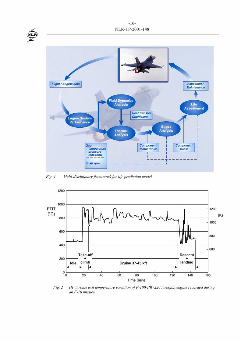
To develop a life prediction model five main disciplines have to be integrated (see Fig.1). Thesedisciplines are applied as follows for a turbine blade:- Engine System Performance Analysis, to determine the operational conditions of the turbine (entry

pressure, temperature, mass flow, rpm) from engine performance history data.- Fluid Dynamic Analysis, to determine the thermal and mechanical loads on a turbine blade

depending on the operational conditions of the turbine.- Thermal Analysis, to calculate the temperature distribution in the blade material.- Stress Analysis, to calculate the thermal and mechanical stresses in the blade material.- Life Consumption Assessment, in particular by fatigue, creep and oxidation.

The analysis tool developed by NLR enables gas turbine operators to optimise their inspection intervals,maintenance planning, component replacement and consequently their costs.

-6-NLR-TP-2001-148

To develop an integrated engine design tool with the disciplines involved would require a massive effortthat would by far exceed the resources at NLR. An analysis tool can however be based upon reverseengineering using experience with existing engines. The present paper will illustrate such an approachtaking the film cooled rotor blades of the high-pressure turbine of the Pratt and Whitney F100-PW-220military turbofan engine as an example. This engine is used by the Royal Netherlands Air Force in theirF-16 fighter aircraft.

The variation of the low-pressure turbine entry temperature (FTIT) measured during a typical F-16mission is shown in figure 2. At take-off FTIT increases from 450 °C (taxi) to 960 °C at full power. Atthe cruise altitude between 37 and 45 kft FTIT varies between 680 °C and 940 °C. During the descenttrong temperature variations occur as a result of frequent changes in power setting.

The present paper will discuss a method to relate the engine operational conditions to the bladetemperature of the first stage rotor of the high pressure turbine. The method combines the results fromavailable software tools to predict the engine thermodynamic performance (the NLR Gas TurbineSimulation Program GSP) and the blade aerodynamics (Numeca’s FINE/Turbo CFD code available atNLR) with engineering estimates of the internal heat transfer and the film cooling efficiency.

The results may be used to address a number of questions such as: what is the blade failure mode (bycreep or fatigue or a combination) and what parts of the mission (and what corresponding powervariations) are most life consuming? Finally, a relative or even absolute life consumption estimate can beestablished to support the engine maintenance activities.

Thermal analysis, stress analysis and the resulting life assessment will not be addressed here but in afuture RTO paper.

2. Approach to predict the blade material temperature

The only information available is the blade geometry and the history of the turbine entry and exitconditions. These conditions are available from recorded flight data, combined with a thermodynamicmodel of the engine to be discussed later. From this information a realistic estimate should be made of theblade temperature and stress history.

The heat transfer calculations are complicated by the fact that the blades are film cooled by high pressureair from the compressor bleed. This air is heated inside the blade before being ejected at a temperature Tinjthrough cooling orifices into the outer flow to provide a cooling air layer with effective temperature Tfilmbetween the blade surface with temperature Tw,ext and the outer hot gas flow.

The external heat transfer qext (W/m2) in the case of film cooling can be expressed as ( Ref.1):

qext = hext (Tfilm − Tw,ext)

It is a well accepted engineering approach to assume that the value of the heat transfer coefficient hext isnot affected by the presence of blade film cooling (Ref.1). In that case hext values can be calculated bywell established CFD methods for zero film cooling.

As a result of the discrete point injection and the mixing with the outer flow Tfilm is somewhere betweenthe adiabatic wall temperature without film cooling and Tinj. This is expressed by the film coolingefficiency:

injgas

filmgasfilm TT

TT−−

=η

Here Tgas is the adiabatic wall temperature without film cooling or, in the case of multiple orifice rowsTgas = Tfilm just upstream of the orifice row (Ref.2). Orifice diameters on the blades considered here are ofthe order of 0.3 mm and orifice rows are typically 6 mm apart. The film cooling efficiency will depend onthe streamwise distance behind the orifice row and on the lateral (spanwise) distance (Ref.1). As a first

-7-NLR-TP-2001-148

simplification, a lateral average may be used. Typical values are of the order of 0.2 close to the orificerow decreasing to 0.1 at 50 orifice diameters downstream (see for instance Ref.1, 3).

A further simplification is to replace the orifice row by a narrow slot of width w with the same cooling airmass flow. FINE/Turbo was recently extended with such a slot film cooling model but during itsapplication a number of practical problems were encountered:• The cooling slots have a width equal to the local grid cell length that was about 5 percent of the blade

chord in the mid-chord region. Film temperatures tend to decrease 2 grid cells ahead of the slot dueto numerical diffusion. Smaller grids are required for sufficient resolution but have not been used toavoid unacceptable long computation times.The slot cooling model will provide cooling efficienciesthat are significantly higher than for orifice cooling near to the orifice rows. This could becompensated for by choosing a higher injection temperature than for the orifice cooling.

FINE/Turbo was therefore used to calculate hext without film cooling to be used for the calculations withfilm cooling. The option of slot film cooling was used only to improve the prediction of the pressuredistribution.

To calculate the external heat transfer, also the film temperature must be determined. This requires arealistic estimate of the film cooling efficiency. In combination with a prediction for the internal heattransfer the blade temperature distribution can be calculated in an iterative procedure with a FiniteElement Method (FEM) model of the blade, starting with an assumed blade temperature distribution. It isnoted that the injection temperature follows from the internal heat transfer to the cooling air but in turnthe injection temperature affects the film temperature and hence the external heat transfer and thus theblade temperature and thus the heating of the cooling air etc., resulting in an iterative procedure.

For the internal cooling an engineering model based on fully developed pipe flow has been used takinginto account the effect of turbulators that increase friction losses and heat transfer. Some of the coolingducts have orifices that provide the external film cooling. Pressure losses and heat transfer in the orificescan be taken into account again by an engineering prediction.

For calculation of the temperature and the heat conduction in the blade material the computer programsMARC or B2000 are available based on finite element methods.

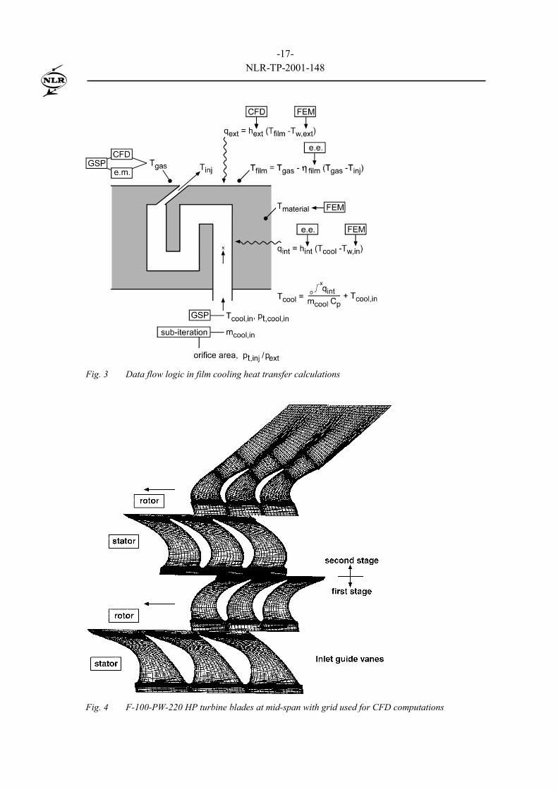
Figure 3 summarises the approach that will be used, depicting the data flow logic. Data processors areindicated in rectangles. Here ‘e.m.’ stands for engineering methods that are well established and ‘e.e.’ forengineering estimates. These estimates constitute the weakest elements in the method and should bevaried in a sensitivity analysis. The estimates relate to (i) the influence of the turbulators and centrifugalforces on internal heat transfer in the serpentine cooling ducts and (ii) to the film cooling efficiency. Thenext chapters will discuss this approach and some results in more detail.

3. From flight data to turbine entry and exit conditions

For assessment of the blade life, the blade temperature history and the resulting stresses must be known.The engine operational data obtained during a particular flight mission form the starting point.

F-16 fighter aircraft of the RNLAF are being equipped with a fatigue analysis system developed by NLR,combined with the Autonomous Combat Evaluation (ACE) system to form the FACE system. Presentlymore than 100 aircraft have an operational FACE system. The relevant signals stored by the FACE DataRecording Unit are engine parameters from the Digital Electronic Engine Control (DEEC) and avionicsdata. The following relevant data are stored: fuel flow to the core engine, fuel flow to the afterburner,exhaust nozzle position (area) and for the flight conditions: Mach, pressure altitude and air temperature.The DEEC signals can be sampled at a maximum frequency of 4 Hz.

These data are used as input data for the Gas Turbine Simulation Program (GSP). This is a tool for gasturbine performance analysis, developed at NLR (Ref.4). This program enables both steady state andtransient simulations for any kind of gas turbine configuration. The simulation is based on one-

-8-NLR-TP-2001-148

dimensional modelling of the processes in the various gas turbine components with thermodynamicrelations and steady-state characteristics (component maps). For the F100-PW-220 engine the componentmaps are based on information from the manufacturer, literature data, and test bench data using reverseengineering. Real gas effects are included as well as thermal and mechanical inertia that are important toaccurately describe the engine transients.

For the current application, GSP is used to calculate the high-pressure turbine entry (station 4) and exit(station 45) total temperature, total pressure and mass flows including the cooling air supplied to the HPturbine. The fuel flows and nozzle position input data are replaced by the Power Lever Angle (PLA)signal, as obtained from FACE. GSP contains a model of the F100-PW-220 engine control unit, whichtranslates the PLA to the appropriate fuel flows and nozzle area. With the engine geometry data also theflow velocities at station 4 and 45 can be calculated, assuming a uniform pressure and temperature.

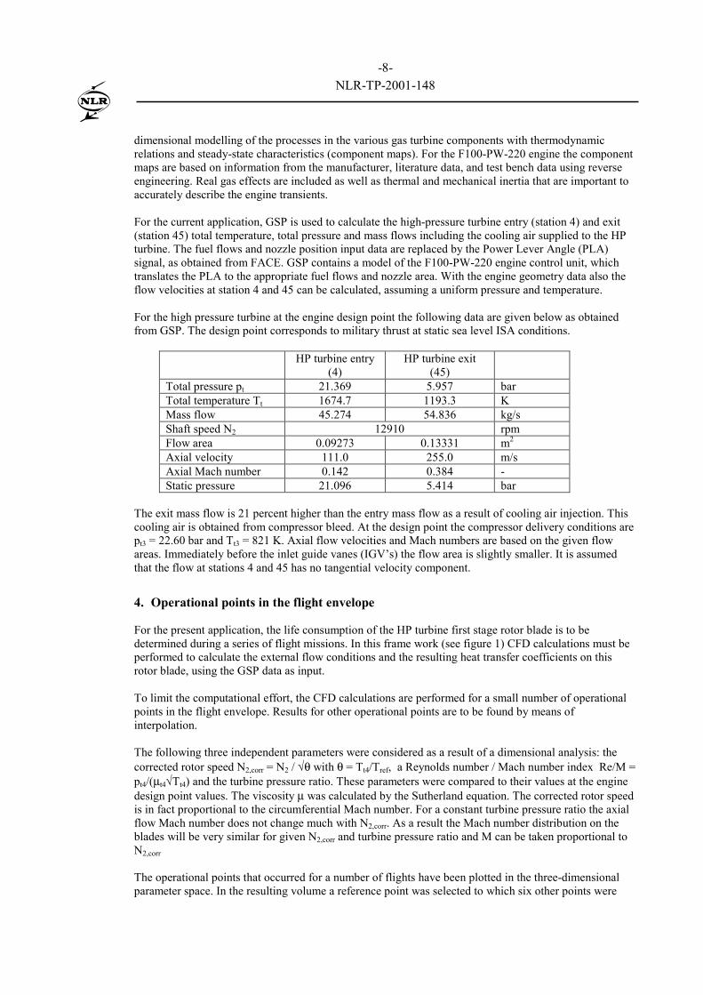
For the high pressure turbine at the engine design point the following data are given below as obtainedfrom GSP. The design point corresponds to military thrust at static sea level ISA conditions.

HP turbine entry(4)

HP turbine exit(45)

Total pressure pt 21.369 5.957 barTotal temperature Tt 1674.7 1193.3 KMass flow 45.274 54.836 kg/sShaft speed N2 12910 rpmFlow area 0.09273 0.13331 m2

Axial velocity 111.0 255.0 m/sAxial Mach number 0.142 0.384 -Static pressure 21.096 5.414 bar

The exit mass flow is 21 percent higher than the entry mass flow as a result of cooling air injection. Thiscooling air is obtained from compressor bleed. At the design point the compressor delivery conditions arept3 = 22.60 bar and Tt3 = 821 K. Axial flow velocities and Mach numbers are based on the given flowareas. Immediately before the inlet guide vanes (IGV’s) the flow area is slightly smaller. It is assumedthat the flow at stations 4 and 45 has no tangential velocity component.

4. Operational points in the flight envelope

For the present application, the life consumption of the HP turbine first stage rotor blade is to bedetermined during a series of flight missions. In this frame work (see figure 1) CFD calculations must beperformed to calculate the external flow conditions and the resulting heat transfer coefficients on thisrotor blade, using the GSP data as input.

To limit the computational effort, the CFD calculations are performed for a small number of operationalpoints in the flight envelope. Results for other operational points are to be found by means ofinterpolation.

The following three independent parameters were considered as a result of a dimensional analysis: thecorrected rotor speed N2,corr = N2 / √θ with θ = Tt4/Tref, a Reynolds number / Mach number index Re/M =pt4/(µt4√Tt4) and the turbine pressure ratio. These parameters were compared to their values at the enginedesign point values. The viscosity µ was calculated by the Sutherland equation. The corrected rotor speedis in fact proportional to the circumferential Mach number. For a constant turbine pressure ratio the axialflow Mach number does not change much with N2,corr. As a result the Mach number distribution on theblades will be very similar for given N2,corr and turbine pressure ratio and M can be taken proportional toN2,corr

The operational points that occurred for a number of flights have been plotted in the three-dimensionalparameter space. In the resulting volume a reference point was selected to which six other points were

-9-NLR-TP-2001-148

added to be used for a tri-linear interpolation. In the next table the parameters for the seven operationalpoints for the CFD calculations are given relative to the engine design point.

Operational point N2,corr Re/M index PRHPTReference point 1 1 1N2C −−−− 1.005 1.342 1.195

0.804 1.342 1.195N2C + 1.155 1.342 1.195Re/M −−−− 1.005 0.783 1.195Re/M − − 1.005 0.391 1.195PR −−−− 1.005 1.342 1.049PR −−−− −−−− 1.005 1.342 0.747

The heat transfer coefficients are calculated in terms of (dimensionless) Stanton numbers

pext

cuh

Stρ

=

Each point in the three-dimensional parameter space corresponds to a single value of the Mach numberdistribution in the turbine. For the present application the product of density and speed of sound at theturbine entry stagnation conditions as defined by (pt4, Tt4) are conveniently used as value for ρu, resultinginto

( )4tp4t

extT/cp

ht~S =

5. The cooling air mass flow distribution in the high-pressure turbine

To predict the effect of mass flow addition by cooling air in the turbine, the distribution of the cooling airin the various stages must be determined, the total amount being given by GSP.

Figure 4 shows the computational grid of the stator and rotor blade sections of the high-pressure turbinenear the mid-span radius (r = 0.28 m). This grid is used for the CFD calculations. The tapered inlet guidevanes have a chord length of 49 mm. The first stage rotor blades are about 46 mm long and have a nearlyconstant chord of 35 mm. As shown in figure 5, the IGV’s and the rotor blades of the first stage have anextensive coverage of film cooling orifices, in particular near the leading edge, the full pressure side andthe forward part of the suction side. To enhance the film coverage, the orifices near the leading edge areoriented towards the spanwise direction. The second stage vanes and blades have no film cooling but onlyinternal air cooling. Except for the second stage rotor blades, the trailing edges are cooled by air blownfrom slots at the pressure side a few mm upstream of the trailing edge.

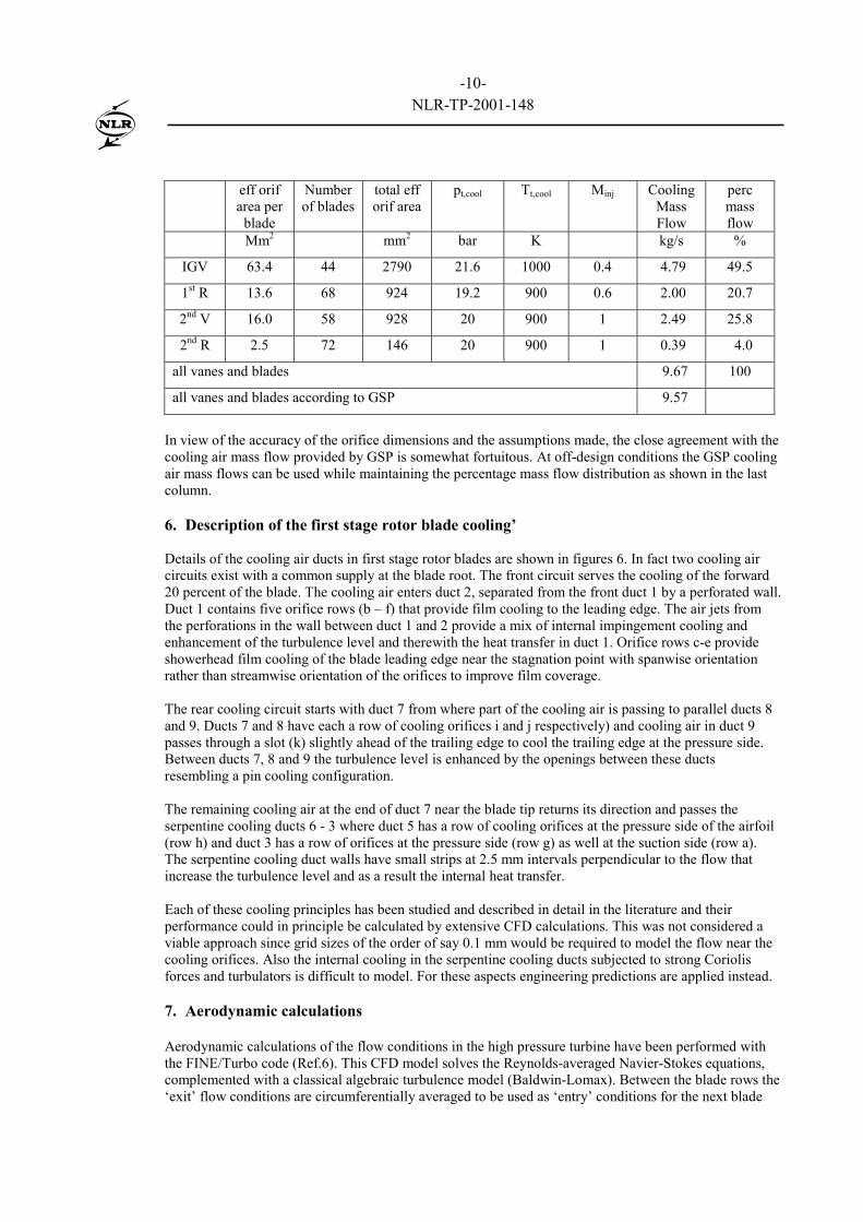
The cooling air distribution was estimated by measuring and counting the film cooling orifices on samplevanes and blades. Orifice diameters varied between 0.25 and 0.4 mm. Measurement accuracy was 0.05mm. The effective orifice area was taken as 80 percent of the geometric area which is a realistic value forpressure ratios pt,cool/pext ≈ 2 (choked orifice flow) with external cross flow (Ref.5). Considering theexternal pressures on the various blades and vanes, an average orifice flow Mach number 0.4 was chosenfor the inlet guide vanes, 0.6 for the first stage rotor blades and for the other blades sonic orifice flow wasassumed. Average total pressures and temperatures just upstream of the orifices had to be estimated,taking into account internal pressure losses and heat transfer. The result is shown in the next table, usingγ = 4/3 for the specific heat ratio.

-10-NLR-TP-2001-148

eff orifarea per

blade

Numberof blades

total efforif area

pt,cool Tt,cool Minj CoolingMassFlow

percmassflow

Mm2 mm2 bar K kg/s %

IGV 63.4 44 2790 21.6 1000 0.4 4.79 49.5

1st R 13.6 68 924 19.2 900 0.6 2.00 20.7

2nd V 16.0 58 928 20 900 1 2.49 25.8

2nd R 2.5 72 146 20 900 1 0.39 4.0

all vanes and blades 9.67 100

all vanes and blades according to GSP 9.57

In view of the accuracy of the orifice dimensions and the assumptions made, the close agreement with thecooling air mass flow provided by GSP is somewhat fortuitous. At off-design conditions the GSP coolingair mass flows can be used while maintaining the percentage mass flow distribution as shown in the lastcolumn.

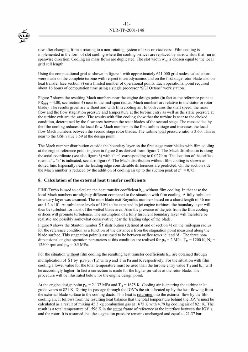
6. Description of the first stage rotor blade cooling’

Details of the cooling air ducts in first stage rotor blades are shown in figures 6. In fact two cooling aircircuits exist with a common supply at the blade root. The front circuit serves the cooling of the forward20 percent of the blade. The cooling air enters duct 2, separated from the front duct 1 by a perforated wall.Duct 1 contains five orifice rows (b – f) that provide film cooling to the leading edge. The air jets fromthe perforations in the wall between duct 1 and 2 provide a mix of internal impingement cooling andenhancement of the turbulence level and therewith the heat transfer in duct 1. Orifice rows c-e provideshowerhead film cooling of the blade leading edge near the stagnation point with spanwise orientationrather than streamwise orientation of the orifices to improve film coverage.

The rear cooling circuit starts with duct 7 from where part of the cooling air is passing to parallel ducts 8and 9. Ducts 7 and 8 have each a row of cooling orifices i and j respectively) and cooling air in duct 9passes through a slot (k) slightly ahead of the trailing edge to cool the trailing edge at the pressure side.Between ducts 7, 8 and 9 the turbulence level is enhanced by the openings between these ductsresembling a pin cooling configuration.

The remaining cooling air at the end of duct 7 near the blade tip returns its direction and passes theserpentine cooling ducts 6 - 3 where duct 5 has a row of cooling orifices at the pressure side of the airfoil(row h) and duct 3 has a row of orifices at the pressure side (row g) as well at the suction side (row a).The serpentine cooling duct walls have small strips at 2.5 mm intervals perpendicular to the flow thatincrease the turbulence level and as a result the internal heat transfer.

Each of these cooling principles has been studied and described in detail in the literature and theirperformance could in principle be calculated by extensive CFD calculations. This was not considered aviable approach since grid sizes of the order of say 0.1 mm would be required to model the flow near thecooling orifices. Also the internal cooling in the serpentine cooling ducts subjected to strong Coriolisforces and turbulators is difficult to model. For these aspects engineering predictions are applied instead.

7. Aerodynamic calculations

Aerodynamic calculations of the flow conditions in the high pressure turbine have been performed withthe FINE/Turbo code (Ref.6). This CFD model solves the Reynolds-averaged Navier-Stokes equations,complemented with a classical algebraic turbulence model (Baldwin-Lomax). Between the blade rows the‘exit’ flow conditions are circumferentially averaged to be used as ‘entry’ conditions for the next blade

-11-NLR-TP-2001-148

row after changing from a rotating to a non-rotating system of axes or vice versa. Film cooling isimplemented in the form of slot cooling where the cooling orifices are replaced by narrow slots that run inspanwise direction. Cooling air mass flows are duplicated. The slot width winj is chosen equal to the localgrid cell length.

Using the computational grid as shown in figure 4 with approximately 621,000 grid nodes, calculationswere made on the complete turbine with respect to aerodynamics and on the first stage rotor blade also onheat transfer (see section 8) on a limited number of operational points. Each operational point requiredabout 16 hours of computation time using a single processor ‘SGI Octane’ work station.

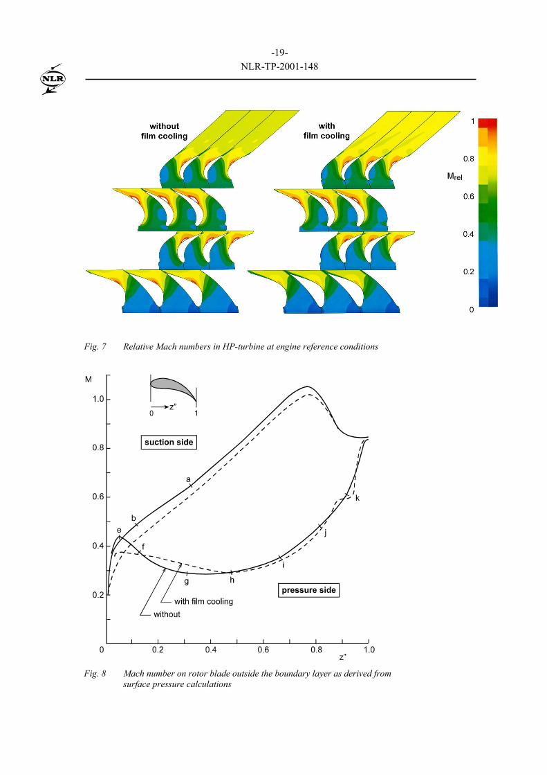
Figure 7 shows the resulting Mach numbers near the engine design point (in fact at the reference point atPRHPT = 4.00, see section 4) near to the mid-span radius. Mach numbers are relative to the stator or rotorblade). The results given are without and with film cooling air. In both cases the shaft speed, the massflow and the flow stagnation pressure and temperature at the turbine entry as well as the static pressure atthe turbine exit are the same. The results with film cooling show that the turbine is near to the chokedcondition, determined by the flow area between the rotor blades of the second stage. The mass added bythe film cooling reduces the local flow Mach numbers in the first turbine stage and increases the localflow Mach numbers between the second stage rotor blades. The turbine total pressure ratio is 3.60. This isnear to the GSP value 3.59 at the design point.

The Mach number distribution outside the boundary layer on the first stage rotor blades with film coolingat the engine reference point is given in figure 8 as derived from figure 7. The Mach distribution is alongthe axial coordinate (see also figure 6) with z′′ =1 corresponding to 0.0279 m. The location of the orificerows ‘a’ .. ‘k’ is indicated, see also figure 6. The Mach distribution without film cooling is shown asdotted line. Especially near the leading edge considerable differences are predicted. On the suction sidethe Mach number is reduced by the addition of cooling air up to the suction peak at z’’ = 0.75.

8. Calculation of the external heat transfer coefficients

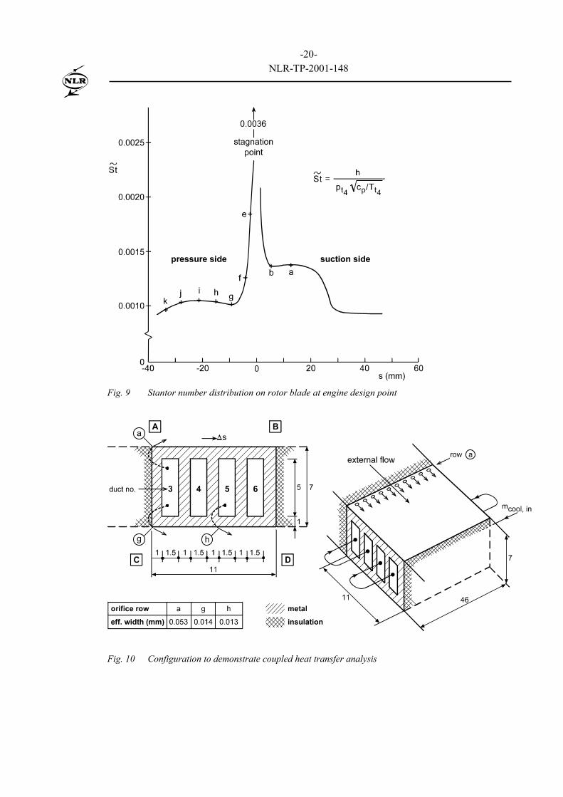
FINE/Turbo is used to calculate the heat transfer coefficient hext without film cooling. In that case thelocal Mach numbers are slightly different compared to the situation with film cooling. A fully turbulentboundary layer was assumed. The rotor blade exit Reynolds numbers based on a chord length of 36 mmare 1.2 × 106. At turbulence levels of 10% to be expected in jet engine turbines, the boundary layer willthen be turbulent for most of the wetted blade area. Also the presence of the jets from the film coolingorifices will promote turbulence. The assumption of a fully turbulent boundary layer will therefore berealistic and possibly somewhat conservative near the leading edge of the blade.Figure 9 shows the Stanton number t~S distribution (defined at end of section 4) on the mid-span radiusfor the reference condition as a function of the distance s from the stagnation point measured along theblade surface. This stagnation point is assumed to be between orifice rows ‘c’ and ‘d’. The three non-dimensional engine operation parameters at this condition are realised for pt4 = 2 MPa, Tt4 = 1200 K, N2 =12500 rpm and p45 = 0.5 MPa.

For the situation without film cooling the resulting heat transfer coefficients hext are obtained throughmultiplication of t~S by pt4√(cp /Tt4) with p and T in Pa and K respectively. For the situation with filmcooling a lower value for the total temperature must be used than the turbine entry value Tt4 and hext willbe accordingly higher. In fact a correction is made for the higher ρu value at the rotor blade. Theprocedure will be illustrated below for the engine design point.

At the engine design point pt4 = 2.137 MPa and Tt4 = 1675 K. Cooling air is entering the turbine inletguide vanes at 821 K. During its passage through the IGV’s the air is heated up by the heat flowing fromthe external blade surface to the cooling ducts. This heat is returning into the external flow by the filmcooling air. It follows from the resulting heat balance that the total temperature behind the IGV’s must becalculated as a result of mixing 45.3 kg combustion gas at 1675 K with 4.79 kg cooling air of 821 K. Theresult is a total temperature of 1596 K in the stator frame of reference at the interface between the IGV’sand the rotor. It is assumed that the stagnation pressure remains unchanged and equal to 21.37 bar.

-12-NLR-TP-2001-148

The result is that Tt4 = 1596 K and pt4 = 2.137 MPa must be used to calculate h from t~S as presented infigure 10 for the engine design point. For t~S = 0.001 a heat transfer coefficient hext = 1.88 kW/m2/Kresults.

CFD calculations predict a (rotor) relative Mach number 0.270 at the mid-span radius at the entry of therotor computational domain. This results in Tt = 1509 K and pt = 16.75 bar in the rotor frame of referenceat the mid-span radius r = 0.285 m. This temperature can be used as Tgas for the calculation of the filmtemperature for given ηfilm , see section 2.

9. Internal heat transfer and pressure losses

The cooling air flow will be heated on its way through the cooling duct and at the same time its totalpressure will reduce as a result of wall friction. Data from Ref.7 were used to estimate of the effect of theturbulators. It is assumed that for the present turbulator configuration the Stanton number St is increasedby a factor 2 and St/(cf)1/3 by a factor 1.2 compared to the value of a turbulent fully developed pipe flow.So, cf increases by a factor 4.6.

Take for example a serpentine cooling duct with a flow Mach number 0.18 with ρu ≈ 700 (kg/s)/m2. Itscross section is of 1.5 × 5 mm leading to a hydraulic diameter of 2.3 mm. Its length is 46 mm. Thecooling air mass flow is 5.2 g/s at T = 1000 K, p = 18 bar and the Reynolds number Red,hyd is 39 000. Thisleads to a heat transfer coefficient of 6 kW/m2/K. For a temperature difference of 100 K between thecooling air and the duct wall the cooling air temperature will increase 56 K in one duct length. Along thisduct the total pressure decreases by 4.4 percent. These calculations can be improved in further iterationsteps.

Orifice flow pressure losses are estimated at 1.3 percent per diameter length with a turbulent pipe flowmodel. The orifice heat transfer coefficient is estimated at 10 kW/m2/K. Taking ρu ≈ 2200 (kg/s)/m2

(sonic flow, discharge coefficient 0.8), an orifice diameter of 0.25 mm and an orifice length of 10diameters, the cooling air temperature is increased by 16 K across the orifice for 100 K temperaturedifference between the orifice wall and the cooling air.

10. Coupled heat transfer calculations

10.1 Simple geometry modelFor prediction of the temperature distribution in the rotor blade material an iterative calculation procedureis required as described in section 2. Before performing these calculations on the actual rotor blade acomputation was made on the simple configuration shown in figure 10, in fact representing the serpentinecooling ducts running along the full blade length of 46 mm.

The side A-B represents part of the blade suction side and C-D part of the pressure side. Cooling airenters duct 6 at a total pressure and temperature of 19.6 bar and 875 K (602 °C). In duct 5 part of thecooling air is ejected through a row of orifices ‘h’ with a total geometric area of 0.75 mm2. In duct 3 theremaining cooling air is ejected through orifices ‘a’ with a total geometric area of 3.0 mm2 and ‘g’ with atotal geometric area of 0.8 mm2. External total pressure and temperature are 16.75 bar and 1509 K. At thesuction side A-B the local external flow Mach number is 0.6 and at the pressure side C-D this is 0.25. Theexternal heat transfer coefficient is 2.6 kW/m2/K at the suction side A-B and 2 kW/m2/K at the pressureside C-D. This corresponds to t~S = 0.0138 and 0.0106 (see figure 9). The internal heat transfercoefficient in the serpentine ducts is 7 kW/m2/K. This is slightly higher than the value mentioned insection 9. Orifice heat transfer is neglected. Some compensation is found by taking the injectiontemperature for the full row equal to the local total temperature in the end of the cooling duct (i.e. at thelast orifice). The heat conductivity of the blade material is λ = 20 W/m/K.

-13-NLR-TP-2001-148

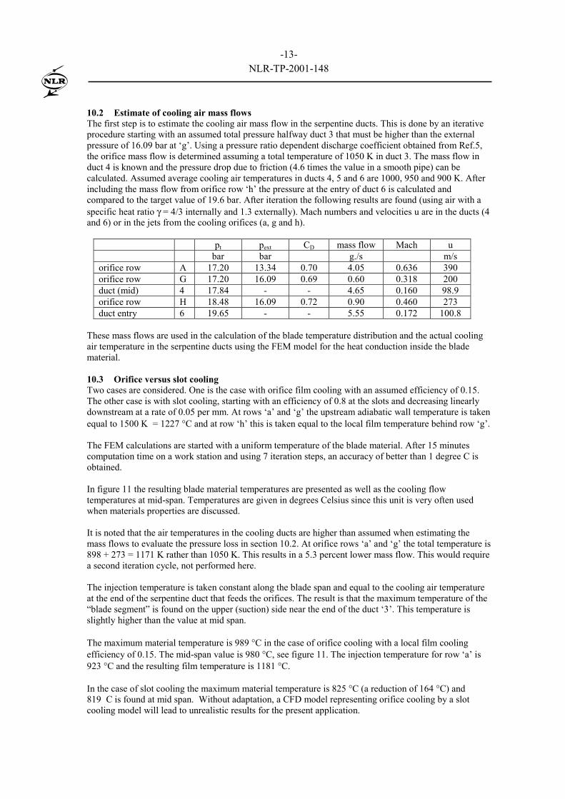
10.2 Estimate of cooling air mass flowsThe first step is to estimate the cooling air mass flow in the serpentine ducts. This is done by an iterativeprocedure starting with an assumed total pressure halfway duct 3 that must be higher than the externalpressure of 16.09 bar at ‘g’. Using a pressure ratio dependent discharge coefficient obtained from Ref.5,the orifice mass flow is determined assuming a total temperature of 1050 K in duct 3. The mass flow induct 4 is known and the pressure drop due to friction (4.6 times the value in a smooth pipe) can becalculated. Assumed average cooling air temperatures in ducts 4, 5 and 6 are 1000, 950 and 900 K. Afterincluding the mass flow from orifice row ‘h’ the pressure at the entry of duct 6 is calculated andcompared to the target value of 19.6 bar. After iteration the following results are found (using air with aspecific heat ratio γ = 4/3 internally and 1.3 externally). Mach numbers and velocities u are in the ducts (4and 6) or in the jets from the cooling orifices (a, g and h).

pt pext CD mass flow Mach ubar bar g./s m/s

orifice row A 17.20 13.34 0.70 4.05 0.636 390orifice row G 17.20 16.09 0.69 0.60 0.318 200duct (mid) 4 17.84 - - 4.65 0.160 98.9orifice row H 18.48 16.09 0.72 0.90 0.460 273duct entry 6 19.65 - - 5.55 0.172 100.8

These mass flows are used in the calculation of the blade temperature distribution and the actual coolingair temperature in the serpentine ducts using the FEM model for the heat conduction inside the bladematerial.

10.3 Orifice versus slot coolingTwo cases are considered. One is the case with orifice film cooling with an assumed efficiency of 0.15.The other case is with slot cooling, starting with an efficiency of 0.8 at the slots and decreasing linearlydownstream at a rate of 0.05 per mm. At rows ‘a’ and ‘g’ the upstream adiabatic wall temperature is takenequal to 1500 K = 1227 °C and at row ‘h’ this is taken equal to the local film temperature behind row ‘g’.

The FEM calculations are started with a uniform temperature of the blade material. After 15 minutescomputation time on a work station and using 7 iteration steps, an accuracy of better than 1 degree C isobtained.

In figure 11 the resulting blade material temperatures are presented as well as the cooling flowtemperatures at mid-span. Temperatures are given in degrees Celsius since this unit is very often usedwhen materials properties are discussed.

It is noted that the air temperatures in the cooling ducts are higher than assumed when estimating themass flows to evaluate the pressure loss in section 10.2. At orifice rows ‘a’ and ‘g’ the total temperature is898 + 273 = 1171 K rather than 1050 K. This results in a 5.3 percent lower mass flow. This would requirea second iteration cycle, not performed here.

The injection temperature is taken constant along the blade span and equal to the cooling air temperatureat the end of the serpentine duct that feeds the orifices. The result is that the maximum temperature of the“blade segment” is found on the upper (suction) side near the end of the duct ‘3’. This temperature isslightly higher than the value at mid span.

The maximum material temperature is 989 °C in the case of orifice cooling with a local film coolingefficiency of 0.15. The mid-span value is 980 °C, see figure 11. The injection temperature for row ‘a’ is923 °C and the resulting film temperature is 1181 °C.

In the case of slot cooling the maximum material temperature is 825 °C (a reduction of 164 °C) and819 C is found at mid span. Without adaptation, a CFD model representing orifice cooling by a slotcooling model will lead to unrealistic results for the present application.

-14-NLR-TP-2001-148

Figure 12 shows the blade surface temperature distribution at mid-span according to fig.11 and thecorresponding film temperature resulting from the assumed film cooling efficiencies. For both coolingmethods the highest heat transfer is found at the downstream edge (points B and D). At point B a heattransfer of 345 × 2.7 = 932 kW/m2 is found for the orifice cooling model and 318 × 2.7 = 859 kW/m2 forthe slot cooling model.

Temperature gradients in the blade material are of the order of 50 °C/mm and are maximum in the topwall of the first cooling duct where the temperature in the cooling ducts is low. If a flat plate is heated onone side such that a temperature difference of 50 °C exists between the two sides and this plate is forcedto remain planar, thermal stresses will develop. For a thermal expansion coefficient ε = 13 E-6 per deg Cand a Youngs modulus E = 2.0 E+5 N/mm2 a stress level is calculated of 65 / 0.7 = 93 N/mm2. Thesematerial values are for a nickel alloy at room temperature. At higher temperatures E may be lower but thisexample illustrates that significant thermal stresses will exist that have to be analysed further and berelated to creep and thermal fatigue, also taking into account the aerodynamic and centrifugal loads thatoccur.

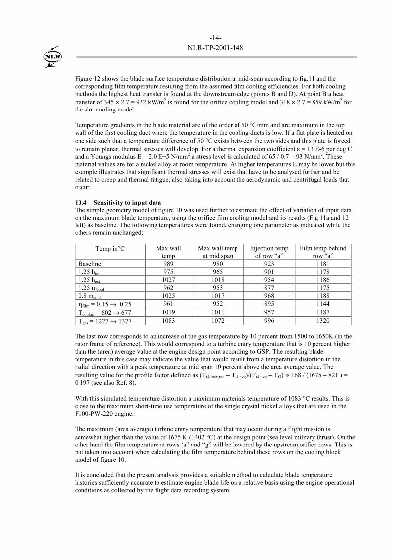
10.4 Sensitivity to input dataThe simple geometry model of figure 10 was used further to estimate the effect of variation of input dataon the maximum blade temperature, using the orifice film cooling model and its results (Fig 11a and 12left) as baseline. The following temperatures were found, changing one parameter as indicated while theothers remain unchanged:

Temp in°C Max walltemp

Max wall tempat mid span

Injection tempof row “a”

Film temp behindrow “a”

Baseline 989 980 923 11811.25 hint 975 965 901 11781.25 hext 1027 1018 954 11861.25 mcool 962 953 877 11750.8 mcool 1025 1017 968 1188ηfilm = 0.15 → 0.25 961 952 895 1144Tcool,in = 602 → 677 1019 1011 957 1187Tgas = 1227 → 1377 1083 1072 996 1320

The last row corresponds to an increase of the gas temperature by 10 percent from 1500 to 1650K (in therotor frame of reference). This would correspond to a turbine entry temperature that is 10 percent higherthan the (area) average value at the engine design point according to GSP. The resulting bladetemperature in this case may indicate the value that would result from a temperature distortion in theradial direction with a peak temperature at mid span 10 percent above the area average value. Theresulting value for the profile factor defined as (Tt4,max,rad − Tt4,avg)/(Tt4,avg − Tt3) is 168 / (1675 − 821 ) =0.197 (see also Ref. 8).

With this simulated temperature distortion a maximum materials temperature of 1083 °C results. This isclose to the maximum short-time use temperature of the single crystal nickel alloys that are used in theF100-PW-220 engine.

The maximum (area average) turbine entry temperature that may occur during a flight mission issomewhat higher than the value of 1675 K (1402 °C) at the design point (sea level military thrust). On theother hand the film temperature at rows ‘a” and “g” will be lowered by the upstream orifice rows. This isnot taken into account when calculating the film temperature behind these rows on the cooling blockmodel of figure 10.

It is concluded that the present analysis provides a suitable method to calculate blade temperaturehistories sufficiently accurate to estimate engine blade life on a relative basis using the engine operationalconditions as collected by the flight data recording system.

-15-NLR-TP-2001-148

11. Conclusions

A method has been formulated to predict the temperature distribution in film cooled turbine blades. Inputdata are: the engine operational conditions and the geometry of the vanes and blades including the sizeand location of the film cooling orifices.

The input data are used as follows:1. The Gas Turbine Simulation Program GSP translates the operational conditions in turbine entry and

exit temperatures, pressures and mass flows including cooling air.2. The distribution of the cooling air between the various blade rows is estimated from the orifice area

and assumed cooling air pressures and temperatures inside the blades.3. FINE/Turbo calculates the pressure and heat transfer coefficient distribution on the rotor blade

without film cooling as well as the pressure distribution with film cooling using turbine entry andexit conditions from GSP. These heat transfer coefficients are also used for the situation with filmcooling.

4. The internal heat transfer and pressure losses are estimated taking the values in fully developedturbulent pipe flows multiplied by factors to account for the presence of turbulators. These factorsare typically 2 and 5 respectively.

5. The film cooling efficiency is a free variable and is typically 0.2 to 0.1 for orifice film cooling.

The following lessons have been learned:1. CFD methods require very fine computational grids to realistically capture the flow and heat

transfer near the film cooling injection orifices. At present this leads to computation times that areout-of-balance with an analysis that relates engine operational conditions during a flight mission toblade temperatures.

2. Modelling cooling orifices by means of a slot width of 1 to 5 percent of the blade chord can be usedefficiently to calculate the effect of added mass by film cooling on the blade pressure distributions.

3. The value of film cooling efficiency is one of the most uncertain factors in the prediction of theblade temperatures when real blades with cooling orifices of optimised orientation are considered.The maximum materials temperature predicted with an orifice cooling efficiency of 0.15 is close tothe maximum short-time use temperature of single crystal nickel alloys.

5. The present analysis provides a suitable method to calculate blade temperature histories sufficientlyaccurate to estimate engine blade life on a relative basis using the engine operational conditions ascollected by the flight data recording system.

12. References

1. Colladay, R.S.; Turbine Cooling, Chapter 11 in: Turbine Design and Application, NASA SP-290(1994).

2. Sellers, J.P.; Gaseous Film Cooling with Multiple Injection Stations, AIAA J. Sept. 1963, pp. 2154-2156.

3. Kadotani, K, and Goldstein, R.J.; Effect of Mainstream Variables on Jets Issuing from a Row ofInclined Round Holes J. Eng. for Power, April 1979, Vol. 101, pp 298-304.

4. Visser, W.P.J.; GSP, A Generic Object-Oriented Gas Turbine Simulation Environment, ASME-2000-GT-0002, NLR-TP-2000-267.

5. Gritsch, M., Schultz, A. and Wittig, S.; Method for Correlating Discharge Coefficients of FilmCooling Holes, AIAA J Vol.36, No.6, June 1998, pp 976-980).

6. Numeca International, FINE/Turbo User Manual (version 4.1), Numeca International, Brussels,April 2000.

7. Harasgama, S.P.; Aerothermal Aspects in Gas Turbine Flows: Turbine Blade Internal Cooling, VKILecture Series 1995-05.

8. Van Erp, C.A. and Richman, M.H.; Technical Challenges Associated with the Development ofAdvanced Combustion Systems, Paper 3 in RTO-MP-14, 1999.

-16-NLR-TP-2001-148

Fig. 1 Multi-disciplinary framework for life prediction model

Fig. 2 HP turbine exit temperature variation of F-100-PW-220 turbofan engine recorded duringan F-16 mission

-17-NLR-TP-2001-148

Fig. 3 Data flow logic in film cooling heat transfer calculations

Fig. 4 F-100-PW-220 HP turbine blades at mid-span with grid used for CFD computations

-18-NLR-TP-2001-148

Fig. 5 F-100-PW-220 high-pressure turbine inlet guide vanes and first stage rotor blade

Fig. 6 First stage rotor blade with cooling ducts and film cooling orifices

-19-NLR-TP-2001-148

Fig. 7 Relative Mach numbers in HP-turbine at engine reference conditions

Fig. 8 Mach number on rotor blade outside the boundary layer as derived fromsurface pressure calculations

-20-NLR-TP-2001-148

Fig. 9 Stantor number distribution on rotor blade at engine design point

Fig. 10 Configuration to demonstrate coupled heat transfer analysis

-21-NLR-TP-2001-148

Fig.11a Temperature distribution at midspan with orifice cooling

Fig.11b Temperature distribution at midspan with slot cooling

-22-NLR-TP-2001-148

Fig. 12 Blade surface and film temperatures for orifice (left) and slot (right) cooling model