Analysis of Cost and Performance - University Of...

Memory Systems: Cache, DRAM, Disk — 6/9/06

981

Copyright 2005 Elsevier Science. Permission to copy must be obtained in writing from the Publisher.

CHAPTER 30

Analysis of Cost and Performance

The characterization of different machine configurations is at the heart of com-puter-system design, and so it is vital that we as practitioners do it correctly. Accu-rate and precise characterizations can provide deep insight into system behavior,enable correct decision making, and ultimately save money and time. Failure toaccurately and precisely describe the system under study can lead to misinterpreta-tions of behavior, misdirected attention, and loss of time and revenue. This chapterdiscusses some of the metrics and tools used in computer-system analysis anddesign, from the correct form of combined multi-metric figures of merit to the phi-losophy of performance characterization.

30.1 Combining Cost and Performance

The following will be obvious in retrospect, but it quite clearly needs to be said,because all too frequently work is presented that unintentionally obscures informa-tion: when combining

cost

and

performance

metrics into a single figure of merit,one must take care to treat the separate metrics appropriately. The same reasoningpresented in this section lies behind other well-known metric-combinations such asenergy-delay product and power-delay product.

To be specific, if combining performance and cost into a single figure of merit, onecan only divide cost into performance if the choice of metric for performance

CHAPTER 30: ANALYSIS OF COST AND PERFORMANCE

982


grows in the opposite direction as the metric for cost. For example, consider the fol-lowing:

•

Bandwidth per pin

•

MIPS per square millimeter

•

Transactions per second per dollar

Bandwidth is good if it increases, while pin count is good if it decreases. MIPS isgood if it increases, while die area (square millimeters) is good if it decreases.Transactions per second is good if it increases, while dollar cost is good it ifdecreases. The combined metrics give information about the value of the designthey represent, in particular how that design might scale. The figure of merit

band-width per pin

suggests that twice the bandwidth can be had for twice the cost (i.e.,doubling the number of pins); the figure of merit

IPC per square millimeter

sug-gests that twice the performance can be had by doubling the number of on-chipresources; the figure of merit

transactions per second per dollar

suggests that thecapacity of the transaction-processing system can be doubled by doubling thecost of the system; and, to a first order, these implications tend to be true.

If we try to combine performance and cost metrics that grow in the same direction,we cannot divide one into the other; we must multiply them. For example, considerthe following:

•

Execution time per dollar (bad)

•

CPI per square millimeter (bad)

•

Request latency per pin (bad)

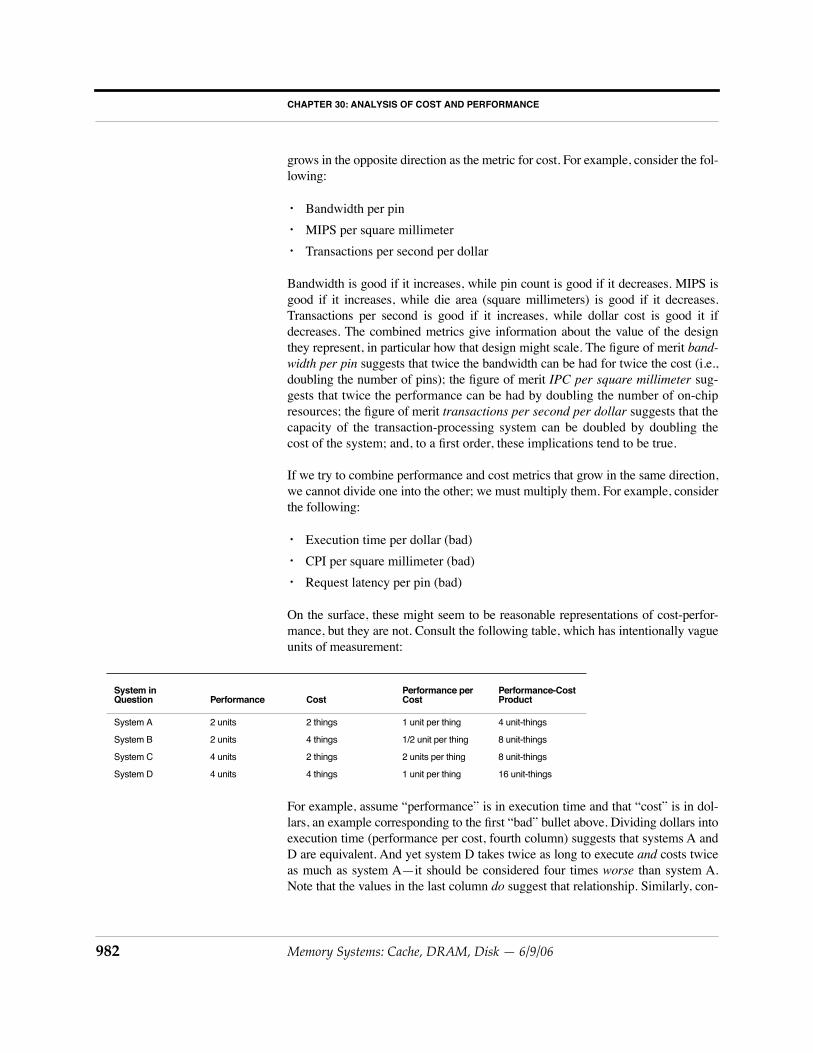
On the surface, these might seem to be reasonable representations of cost-perfor-mance, but they are not. Consult the following table, which has intentionally vagueunits of measurement:

For example, assume “performance” is in execution time and that “cost” is in dol-lars, an example corresponding to the first “bad” bullet above. Dividing dollars intoexecution time (performance per cost, fourth column) suggests that systems A andD are equivalent. And yet system D takes twice as long to execute

and

costs twiceas much as system A—it should be considered four times

worse

than system A.Note that the values in the last column

do

suggest that relationship. Similarly, con-

System in Question Performance Cost

Performance per Cost

Performance-Cost Product

System A 2 units 2 things 1 unit per thing 4 unit-things

System B 2 units 4 things 1/2 unit per thing 8 unit-things

System C 4 units 2 things 2 units per thing 8 unit-things

System D 4 units 4 things 1 unit per thing 16 unit-things


983

30.2 PARETO OPTIMALITY

sider “performance” as CPI and “cost” as die area (second “bad” bullet above).Dividing die area into CPI (performance per cost, fourth column) suggests that sys-tem C is four times worse than system B (its CPI per square millimeter value is fourtimes higher). However, put another way, system C costs half as much as system Bbut has half the performance as B—so the two should be equivalent, which is pre-cisely what is shown in the last column.

Using a performance-cost product instead of a quotient gives the results that areappropriate and intuitive:

•

Execution-time-dollars

•

CPI-square-millimeters

•

Request-latency-pin-count product

Note that, when combining multiple atomic metrics into a single figure of merit,one is really attempting to cast into a single number the information provided in aPareto plot, where each metric corresponds to its own axis. Collapsing a multi-dimensional representation into a single number itself obscures information, even ifdone “correctly,” and thus we would encourage a designer to always use Paretoplots when possible. This leads us to the following section.

30.2 Pareto Optimality

This section reproduces part of the

Overview

chapter, for the sake of completeness.

The Pareto-Optimal Set: an Equivalence Class

It is convenient to represent the “goodness” of a design solution, a particular systemconfiguration, as a single number so that one can readily compare the number withthe “goodness” ratings of other candidate design solutions and thereby quickly findthe “best” system configuration. However, in the design of memory systems, we areinherently dealing with a multi-dimensional design space (e.g., one that encom-passes performance, energy consumption, cost, etc.), and so using a single numberto represent a solution’s worth is not really appropriate, unless we assign exactweights to the various metrics (which is dangerous and will be discussed in moredetail later) or unless we care about one aspect to the exclusion of all others (e.g.,performance at any cost).

Assuming that we do not have exact weights for the figures of merit and that we docare about more than one aspect of the system, a very powerful tool to aid in system


984


analysis is the concept of

Pareto optimality

or

Pareto efficiency

, named after theItalian economist, Vilfredo Pareto, who invented it in the early 1900’s.

Pareto optimality asserts that one candidate solution to a problem is better thananother candidate solution only if the first

dominates

the second: i.e., if the first isbetter than or equal to the second in

all

figures of merit. If one solution has a bettervalue in one dimension but a worse value in another, then the two candidates arePareto-equivalent. The “best” solution is actually a set of candidate solutions: theset of Pareto-equivalent solutions that are not dominated by any solution.

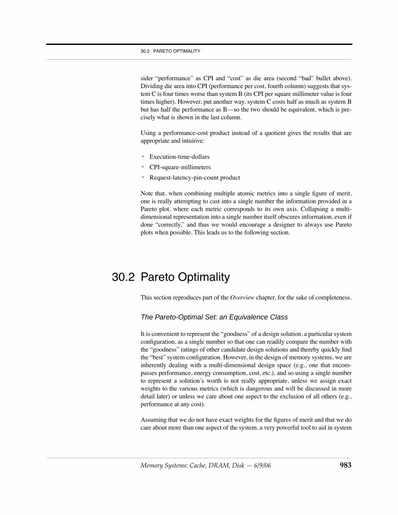
Figure 30.1 illustrates. Figure 30.1(a) shows a set of candidate solutions in a two-dimensional space that represents a cost/performance metric: in this example, thex-axis represents system performance in execution time (smaller numbers are bet-ter), and the y-axis represents system cost in dollars (smaller numbers are better).Figure 30.1(b) shows the Pareto-optimal set in solid black and connected by a line;

FIGURE 30.1: Pareto optimality. Members of the Pareto-optimal set are shown in solid black; non-optimal points aregrey.

Execution time

Cost

Execution time

Cost

Execution time

Cost

A

B

C

D

Execution time

Cost

(a) a set of data points (b) the Pareto-optimal wavefront

(c) addition of four new points to data set (d) the new Pareto-optimal wavefront

A

B

C

D


985

30.2 PARETO OPTIMALITY

the line denotes the boundary between the Pareto-optimal subset and the dominatedsubset, with points on the line belonging to the dominated set (dominated datapoints are shown in the figure as grey). In this example, the Pareto-optimal setforms a wavefront that approaches both axes simultaneously. Figures 30.1(c) and30.1(d) show the effect of adding four new candidate solutions to the space: onelies inside the wavefront, one lies on the wavefront, and two lie outside the wave-front. The first two new additions, A and B, are both dominated by at least onemember of the Pareto-optimal set, and so neither is considered Pareto-optimal.Even though B lies on the wavefront, it is not considered Pareto-optimal: the pointto the left of B has better performance than B at equal cost, and thus it dominates B.

The point C is not dominated by any member of the Pareto-optimal set, nor does itdominate any member of the Pareto-optimal set; thus, candidate-solution C isadded to the optimal set, and its addition changes the shape of the wave-frontslightly. The last of the additional points, D, is dominated by no members of theoptimal set, but it

does

dominate several members of the optimal set, so D’s inclu-sion in the optimal set excludes those dominated members from the set. As a result,candidate-solution D changes the shape of the wave-front more significantly thandid candidate-solution C.

The primary benefit of using Pareto analysis is that, by definition, the individualmetrics along each axis are considered independently. Unlike the combination met-rics of the previous section, a Pareto graph embodies no implicit evaluation of therelative importance between the various axes. For example, if a 2D Pareto graphplots cost on one axis and (execution) time on the other, a combined cost-time met-ric (e.g., the

cost Execution time

product) would collapse the 2D Pareto graph into asingle dimension, with each value

α

in the 1D cost-time space corresponding to allpoints on the curve

y

=

α

/

x

in the 2D Pareto space. The implication of representingthe data set in a 1D metric such as this is that the two metrics

cost

and

time

areequivalent—that one can be traded off for the other in a 1-for-1 fashion. However,as a Pareto plot will show, not all equally

achievable

designs lie on a 1/

x

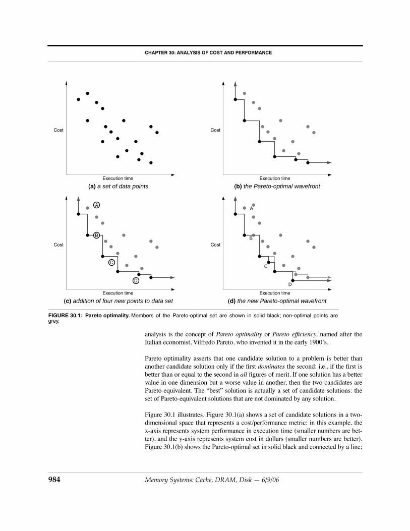
curve.Often, a designer will find that trading off a factor of two in one dimension (cost) togain a factor of two in the other dimension (execution time) fails to scale after apoint or is altogether impossible to begin with. Collapsing the data set into a singlemetric will obscure this fact, while plotting the data in a Pareto graph will not. Fig-ure 30.2 illustrates. Real data reflects realistic limitations, such as a non-equaltrade-off between cost and performance. Limiting the analysis to a combined met-ric in the example data set would lead a designer toward designs that trade off costfor execution time, when perhaps the designer would prefer to choose lower-costdesigns.

A related observation (credited to Tim Stanley, a former graduate student in theUniversity of Michigan’s Advanced Computer Arhitecture Lab) is that require-ments-driven analysis can similarly obscure information and potentially leaddesigners away from optimal choices. When requirements are specified in languagesuch as

not to exceed

some value of some metric (such as power dissipation or diearea or dollar cost), a hard line is drawn that forces a designer to ignore a portion of


986


the design space. However, the observation is that, as far as design explorationgoes, all of the truly interesting designs hover right around that cut-off. Forinstance, if one’s design limitation is

cost not to exceed X

, then all interestingdesigns will lie within a small distance of cost

X

, including small deltas beyond

X

.It is frequently the case that small deltas beyond the cut-off in cost might yield largedeltas in performance. If a designer fails to consider these points, he may overlookthe ideal design.

30.3 Taking Sampled Averages Correctly

In the opening chapter of the book, we discussed this topic and left off with anunanswered question. Here, we present the full discussion and give closure to thereader. Like the previous section, so that this section can stand alone, we repeatmuch of the original discussion.

In many fields, including the field of computer engineering, it is quite popular tofind a

sampled average

—i.e. the average of a sampled set of numbers, rather thanthe average of the entire set. This is useful when the entire set is unavailable, or dif-ficult to obtain, or expensive to obtain. For example, one might want to use thistechnique to keep a running performance average for a real microprocessor, or onemight want to sample several windows of execution in a terabyte-size trace file.Provided that the sampled subset is representative of the set as a whole, and pro-

FIGURE 30.2: Pareto Analysis vs. Combined Metrics. Combining different metrics into a single figure of merit obscures informa-tion. For example, representing the given dataset with a single cost-time product would equate by definition all designs lying on each1/x curve. The 1/x curve shown in solid black would divide the Pareto-optimal set: those designs lying to the left and below the curvewould be considered “better” than those designs lying to the right and above the curve. The design corresponding to data point “A,”given a combined-metric analysis, would be considered superior to the design corresponding to data point “B,” though Pareto analysisindicates otherwise.

Execution time

Cost

y=a/x

A

B

Execution time

Cost


987

30.3 TAKING SAMPLED AVERAGES CORRECTLY

vided that the technique used to collect the samples is correct, this mechanism pro-vides a low-cost alternative that can be very accurate. This section demonstratesthat the technique used to collect the samples can easily be incorrect, and that theresults can be far from accurate, if one follows intuition.

The discussion will use as an example a mechanism that samples the miles-per-gal-lon performance of an automobile under way. The trip we will study is an out &back trip with a brief pit-stop, shown in Figure 30.3. The automobile will follow asimple course that is easily analyzed:

1.

The auto will travel over even ground for 60 miles, at 60 mph, and it will achieve 30 mpg during this window of time.

2.

The auto will travel uphill for 20 miles, at 60 mph, and it will achieve 10 mpg during this window of time.

3.

The auto will travel downhill for 20 miles, at 60 mph, and it will achieve 300 mpg during this window of time.

4.

The auto will travel back home over even ground for 60 miles, at 60 mph, and it will achieve 30 mpg during this window of time.

5.

In addition, before returning home, the driver will sit at the top of the hill for 10 minutes, enjoying the view, with the auto idling, consuming gasoline at the rate of one gallon every 5 hours. This is equivalent to 1/300 gallon per minute, or 1/30 of a gallon during the 10-minute respite. Note that the auto will achieve 0 mpg during this window of time.

Let’s see how we can sample the car’s gasoline efficiency. There are three obviousunits of measurement involved in the process: the trip will last some amount oftime (minutes), the car will travel some distance (miles), and the trip will consumean amount of fuel (gallons). At the very least, we can use each of these units to pro-vide a space over which we will sample the desired metric.

FIGURE 30.3: Course Taken by Automobile in Example.

60 miles, 60 mph, 30 mpg

20 miles, 60 mph

up: 10 mpg

down: 300 mpg

10 minutes idling0 mph, 0 mpg


988


30.3.1 Sampling Over Time

Our first treatment will sample miles-per-gallon over time. Our car’s algorithm willsample evenly in time, so for our analysis we need to break down the segments ofthe trip by the amount of time that they take:

•

Outbound: 60 minutes

•

Uphill: 20 minutes

•

Idling: 10 minutes

•

Downhill: 20 minutes

•

Return: 60 minutes

This is displayed graphically in Figure 30.4, in which the time for each segmentshown to scale. Assume, for the sake of simplicity, that the sampling algorithmsamples the car’s miles-per-gallon every minute and adds that sampled value to therunning average (it could just as easily sample every second or millisecond). Thenthe algorithm will sample the value 30mpg 60 times during the first segment of thetrip; it will sample the value 10mpg 20 times during the second segment of the trip;it will sample the value 0mpg 10 times during the third segment of the trip; and soon. Over the trip, the car is operating for a total of 170 minutes; thus we can derivethe sampling algorithm’s results as follows:

(EQ 30.1)

If we were to believe this method of calculating sampled averages, we wouldbelieve that the car, at least on this trip, is getting roughly twice the fuel efficiencyof traveling over flat ground, despite the fact that the trip started and ended in the

FIGURE 30.4: Sampling MPG Over Time. The figure shows the trip in time, with each segment of time labeled with theaverage miles-per-gallon for car during that segment of the trip. Thus, whenever the sampling algorithm samples MPG dur-ing a window of time, it will add that value to the running average.

60 minutes

30 mpg

60 minutes

30 mpg

20 min

10 mpg

20 min

300 mpg

10 min

0mpg 170 mintotal

60min170min--------------------30mpg +

20min170min--------------------10mpg +

10min170min--------------------0mpg +

20min170min--------------------300mpg +

60min170min--------------------30mpg

57.5mpg=

Points at which samples are taken:10 samples

60170---------30

20170---------10

10170---------0

20170---------300

60170---------30+ + + + 57.5mpg=


989


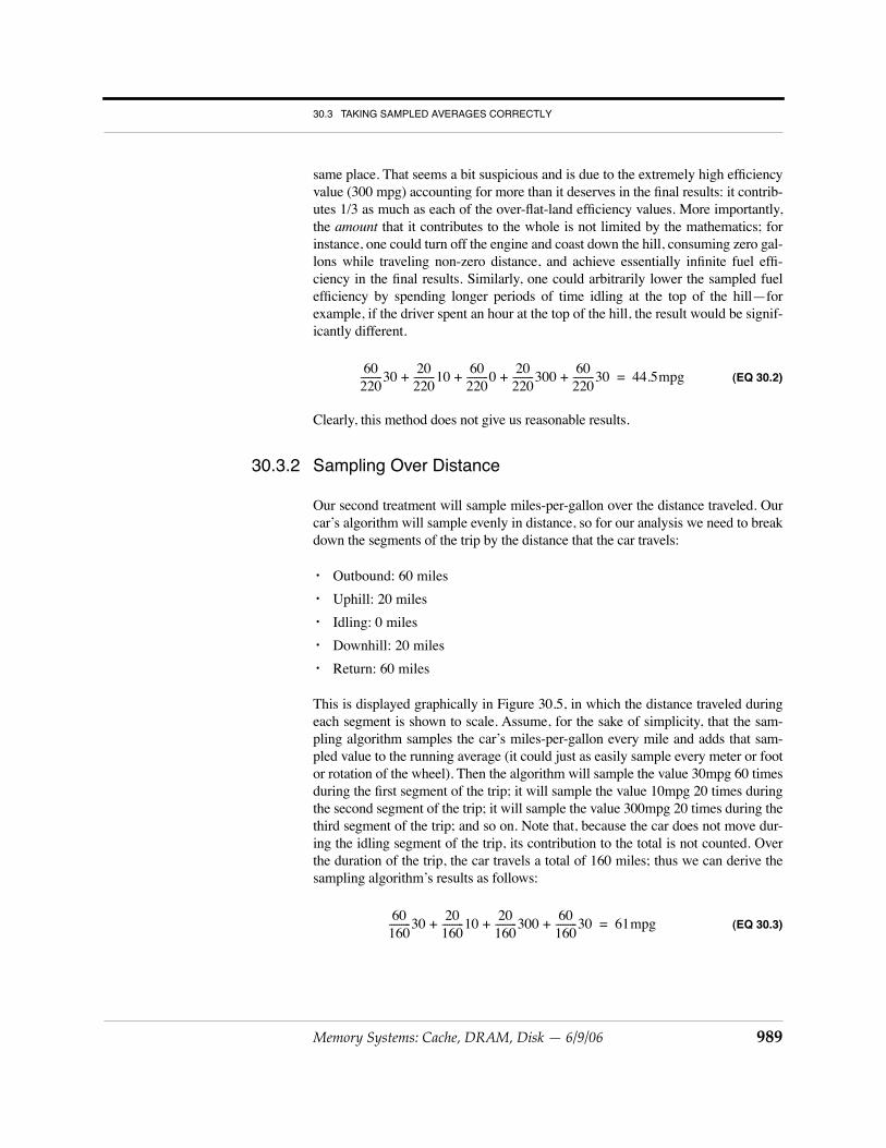
same place. That seems a bit suspicious and is due to the extremely high efficiencyvalue (300 mpg) accounting for more than it deserves in the final results: it contrib-utes 1/3 as much as each of the over-flat-land efficiency values. More importantly,the

amount

that it contributes to the whole is not limited by the mathematics; forinstance, one could turn off the engine and coast down the hill, consuming zero gal-lons while traveling non-zero distance, and achieve essentially infinite fuel effi-ciency in the final results. Similarly, one could arbitrarily lower the sampled fuelefficiency by spending longer periods of time idling at the top of the hill—forexample, if the driver spent an hour at the top of the hill, the result would be signif-icantly different.

(EQ 30.2)

Clearly, this method does not give us reasonable results.

30.3.2 Sampling Over Distance

Our second treatment will sample miles-per-gallon over the distance traveled. Ourcar’s algorithm will sample evenly in distance, so for our analysis we need to breakdown the segments of the trip by the distance that the car travels:

• Outbound: 60 miles

• Uphill: 20 miles

• Idling: 0 miles

• Downhill: 20 miles

• Return: 60 miles

This is displayed graphically in Figure 30.5, in which the distance traveled duringeach segment is shown to scale. Assume, for the sake of simplicity, that the sam-pling algorithm samples the car’s miles-per-gallon every mile and adds that sam-pled value to the running average (it could just as easily sample every meter or footor rotation of the wheel). Then the algorithm will sample the value 30mpg 60 timesduring the first segment of the trip; it will sample the value 10mpg 20 times duringthe second segment of the trip; it will sample the value 300mpg 20 times during thethird segment of the trip; and so on. Note that, because the car does not move dur-ing the idling segment of the trip, its contribution to the total is not counted. Overthe duration of the trip, the car travels a total of 160 miles; thus we can derive thesampling algorithm’s results as follows:

(EQ 30.3)

60220---------30

20220---------10

60220---------0

20220---------300

60220---------30+ + + + 44.5mpg=

60160---------30

20160---------10

20160---------300

60160---------30+ + + 61mpg=


990 Memory Systems: Cache, DRAM, Disk — 6/9/06

This result is not far from the previous result, which should indicate that it, too,fails to gives us believable results. The method falls prey to the same problem asbefore: the large value of 300 mpg contributes significantly to the average, and onecan “trick” the algorithm by using infinite values when shutting off the engine. Theone advantage this method has over the previous method is that one cannot arbi-trarily lower the fuel efficiency by idling longer periods of time: idling is con-strained by the mathematics to be excluded from the average. Idling travels zerodistance, and therefore its contribution to the whole is zero. Yet this is perhaps tooextreme, as idling certainly contributes some amount to an automobile’s fuel effi-ciency.

30.3.3 Sampling Over Fuel Consumption

Our last treatment will sample miles-per-gallon along the axis of fuel consumption.Our car’s algorithm will sample evenly in gallons consumed, so for our analysis weneed to break down the segments of the trip by the amount of fuel that they con-sume:

• Outbound: 60 miles @ 30 mpg = 2 gallons

• Uphill: 20 miles @ 10 mpg = 2 gallons

• Idling: 10 minutes at 1/300 gallon per minute = 1/30 gallon

• Downhill: 20 miles @ 300 mpg = 1/15 gallon

• Return: 60 miles @ 30 mpg = 2 gallons

This is displayed graphically in Figure 30.6, in which the fuel consumed duringeach segment of the trip is shown to scale. Assume, for the sake of simplicity, thatthe sampling algorithm samples the car’s miles-per-gallon every 1/30 gallon andadds that sampled value to the running average (it could just as easily sample every

10 samples

30 mpg 30 mpg10 mpg 300 mpg

FIGURE 30.5: Sampling MPG Over Distance. The figure shows the trip in distance traveled, with each segment of dis-tance labeled with the average miles-per-gallon for car during that segment of the trip. Thus, whenever the sampling algo-rithm samples MPG during a window, it will add that value to the running average.

60miles160miles------------------------30mpg +

20miles160miles------------------------10mpg +

20miles160miles------------------------300mpg +

60miles160miles------------------------30mpg

61mpg=

60 miles 60 miles20 miles 20 miles

160 milestotal

Points at which samples are taken:

Memory Systems: Cache, DRAM, Disk — 6/9/06 991


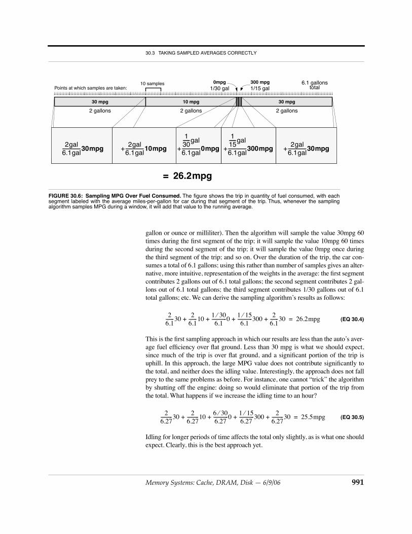
gallon or ounce or milliliter). Then the algorithm will sample the value 30mpg 60times during the first segment of the trip; it will sample the value 10mpg 60 timesduring the second segment of the trip; it will sample the value 0mpg once duringthe third segment of the trip; and so on. Over the duration of the trip, the car con-sumes a total of 6.1 gallons; using this rather than number of samples gives an alter-native, more intuitive, representation of the weights in the average: the first segmentcontributes 2 gallons out of 6.1 total gallons; the second segment contributes 2 gal-lons out of 6.1 total gallons; the third segment contributes 1/30 gallons out of 6.1total gallons; etc. We can derive the sampling algorithm’s results as follows:

(EQ 30.4)

This is the first sampling approach in which our results are less than the auto’s aver-age fuel efficiency over flat ground. Less than 30 mpg is what we should expect,since much of the trip is over flat ground, and a significant portion of the trip isuphill. In this approach, the large MPG value does not contribute significantly tothe total, and neither does the idling value. Interestingly, the approach does not fallprey to the same problems as before. For instance, one cannot “trick” the algorithmby shutting off the engine: doing so would eliminate that portion of the trip fromthe total. What happens if we increase the idling time to an hour?

(EQ 30.5)

Idling for longer periods of time affects the total only slightly, as is what one shouldexpect. Clearly, this is the best approach yet.

Points at which samples are taken:

30 mpg 10 mpg 30 mpg

FIGURE 30.6: Sampling MPG Over Fuel Consumed. The figure shows the trip in quantity of fuel consumed, with eachsegment labeled with the average miles-per-gallon for car during that segment of the trip. Thus, whenever the samplingalgorithm samples MPG during a window, it will add that value to the running average.

2gal6.1gal----------------30mpg +

2gal6.1gal----------------10mpg +

130------gal

6.1gal----------------0mpg +

115------gal

6.1gal----------------300mpg +

2gal6.1gal----------------30mpg

26.2mpg=

2 gallons 2 gallons

1/15 gal300 mpg

1/30 gal0mpg 6.1 gallons

total

2 gallons

10 samples

26.1-------30

26.1-------10

1 30⁄6.1

-------------01 15⁄6.1

-------------3002

6.1-------30+ + + + 26.2mpg=

26.27----------30

26.27----------10

6 30⁄6.27-------------0

1 15⁄6.27-------------300

26.27----------30+ + + + 25.5mpg=



30.3.4 The Moral of the Story

So what is the real answer? The auto travels 160 miles, consuming 6.1 gallons; it isnot hard to find the actual miles-per-gallon achieved.

(EQ 30.6)

The approach that is perhaps the least intuitive (sampling over the space of gal-lons?) does give the correct answer. We see that, if the metric we are measuring ismiles per gallon,

• sampling over minutes (time) is bad;

• sampling over miles (distance) is bad; but

• sampling over gallons (consumption) is good.

Moreover (and perhaps most importantly), in this context, “bad” means “can be offby a factor of two or more.”

The moral of the story is that if you are sampling the following metric:

(EQ 30.7)

then you must sample that metric in equal steps of dimension unit. To wit, if sam-pling the metric miles per gallon, you must sample evenly in units of gallon; ifsampling the metric cycles per instruction, you must sample evenly in units ofinstruction (i.e., evenly in instructions committed, not instructions fetched or exe-cuted*); if sampling the metric instructions per cycle, you must sample evenly inunits of cycle; and if sampling the metric cache miss rate (i.e. cache misses percache access), you must sample evenly in units of cache access.

What does it mean to sample in units of instruction or cycle or cache access? For amicroprocessor, it means that one must have a count-down timer that decrementsevery unit—i.e., once for every instruction committed, or once every cycle, or onceevery time the cache is accessed—and on every epoch (i.e., whenever a predefinednumber of units have transpired) the desired average must be taken. For an automo-bile providing real-time fuel efficiency, a sensor must be placed in the gas line thatinterrupts a controller whenever a predefined unit of volume of gasoline is con-sumed.

* The metrics must match exactly. The common definition of CPI is total execution cycles divided by the total number of instructions performed/committed and does not include speculative instructions in the denominator (though it does include their effects in the numerator).

160miles6.1gallons------------------------- 26.2mpg=

dataunit----------


30.4 METRICS FOR COMPUTER PERFORMANCE

What determines the predefined amounts that set the epoch size? Clearly, to catchall interesting behavior one must sample frequently enough to measure all impor-tant events. Higher sampling rates lead to better accuracy, at a higher cost of imple-mentation. How does sampling at a lower rate affect one’s accuracy? For example,by sampling at a rate of once every 1/30 gallon in the previous example, we wereassured of catching every segment of the trip. However, this was a contrived exam-ple where we knew the desired sampling rate ahead of time. What if, as in normalcases, one does not know the appropriate sampling rate? For example, if the exam-ple algorithm sampled every gallon instead of every small fraction of a gallon, wewould have gotten the following results:

(EQ 30.8)

The answer is off the true result, but it is not as bad as if we had generated the sam-pled average incorrectly in the first place (e.g., sampling in minutes or miles trav-eled).

30.4 Metrics for Computer Performance

This section explains what it means to characterize the performance of a computerand which methods are appropriate and inappropriate for the task. The most widelyused metric is the performance on the SPEC benchmark suite of programs; cur-rently, the results of running the SPEC benchmark suite are compiled into a singlenumber using the geometric mean. The primary reason for using the geometricmean is that it preserves values across normalization, but unfortunately it does notpreserve total run time, which is probably the figure of greatest interest when per-formances are being compared.

Average Cycles per Instruction (average CPI) is another widely used metric, butusing this metric to compare performance is also invalid, even if comparingmachines with identical clock speeds. Comparing averaged CPI values to judgeperformance falls prey to the same problems as averaging normalized values.

Instead of the geometric mean, either the harmonic or the arithmetic mean is theappropriate method for averaging a set running times. The arithmetic mean shouldbe used to average times, and the harmonic mean should be used to average rates*

(“rate” meaning 1/time). In addition, normalized values must never be averaged, asthis section will demonstrate.

26---30

26---10

26---30+ + 23.3mpg=



30.4.1 Performance and the Use of Means

We want to summarize the performance of a computer; the easiest way uses a sin-gle number that can be compared against the numbers of other machines. This typ-ically involves running tests on the machine and taking some sort of mean; themean of a set of numbers is the central value when the set represents fluctuationsabout that value. There are a number of different ways to define a mean value;among them the arithmetic mean, the geometric mean, and the harmonic mean.

The arithmetic mean is defined as follows:

(EQ 30.9)

The geometric mean is defined as follows:

(EQ 30.10)

The harmonic mean is defined as follows

(EQ 30.11)

In the mathematical sense, the geometric mean of a set of n values is the length ofone side of an n-dimensional cube having the same volume as an n-dimensionalrectangle whose sides are given by the n values. As this is neither intuitive norinformative, the wisdom of using the geometric mean for anything is questionable*.Its only apparent advantage is that it is unaffected by normalization: whether one

* A note on rates, in particular miss rate. Even though miss rate is a “rate,” it is not a rate in the harmonic/arithmetic mean sense because (a) it contains no concept of time, and, more importantly, (b) the thing a designer cares about is the number of misses (in the numerator), not the number of cache accesses (in the denominator). The oft-chanted mantra of “use harmonic mean to average rates” only applies to scenarios in which the metric a designer really cares about is in the denominator. For instance, when a designer says “performance” he is really talking about time, and when the metric puts time in the denominator either explicitly (as in the case of instructions per second) or implicitly (as in the case of instructions per cycle), the metric becomes a “rate” int eh harmonic mean sense. For example, if one uses the metric cache-accesses-per-cache-miss, this is a de facto rate, and the harmonic mean would probably be the appropriate mean to use.

ArithmeticMean a1 a2 a3 … aN, , , ,( )

aii

N

∑N

-----------=

GeometricMean a1 a2 a3 … aN, , , ,( ) aii

N

∏N=

HarmonicMean a1 a2 a3 … aN, , , ,( ) N

1a---

ii

N

∑------------=



normalizes by a set of weights first or by the geometric mean of the weights after-ward, the result is the same.

This property has been used to suggest that the geometric mean is superior, since itproduces the same results when comparing several computers irrespective of whichcomputer’s times are used as the normalization factor [Fleming & Wallace 1986].However, the argument was rebutted in [Smith 1988], where the meaninglessnessof the geometric mean was first illustrated.

In this book, we consider only the arithmetic and harmonic means. Since the twoare inverses of each other,

(EQ 30.12)

and since the arithmetic mean—the “average”—is more easily visualized than theharmonic mean, we will stick to the average from now on, relating it back to theharmonic mean when appropriate.

An Example

We begin with a simple illustrative example of what can go wrong when we try tosummarize performance. Rather than demonstrate incorrectness, the intent is toconfuse the issue by hinting at the subtle interactions of units and means.

A machine is timed running two benchmark tests and receives the following scores:

How fast is the machine? Let us look at different ways of calculating performance:

Method 1—one way of looking at this is by the ratios of the running times:

The machine’s performance on test 1 is four times faster than an average machine,its performance on test 2 is twice as fast as average, therefore our machine is (onaverage) three times as fast as most machines.

* Compare this to just one physical interpretation of the arithmetic mean; finding the center of gravity in a set of objects (possibly having different weights) placed along a see-saw. There are countless other interpretations which are just as intuitive and mean-ingful.

test1: 3 sec (most machines run it in 12 seconds)test2: 300 sec (most machines run it in 600 seconds)

ArithmeticMean a1 a2 a3 …, , ,( ) 1

HarmonicMean1a1----- 1

a2----- 1

a3----- …, , ,⎝ ⎠

⎛ ⎞--------------------------------------------------------------------------------=

test1:312------ test2:

300600---------



Method 2—another way of looking at this is by the ratios of the running times:

The machine’s running time on test 1 is 1/4 the time it takes most machines, its run-ning time on test 2 is 1/2 the time it takes most machines, so our machine (on aver-age) takes 3/8 the time a typical machine does to run a program, or, put anotherway, our machine is 8/3 (2.67) times as fast as the average machine.

Method 3—yet another way of looking at this is by the ratios of the running times:

The machine ran the benchmarks in a total of 303 seconds, the average machineruns the benchmarks in 612 seconds, therefore our machine takes 0.495 the amountof time to run the benchmarks as most machines do, and so is roughly twice as fastas the typical machine (on average).

Method 4—and then you can always look at the ratios of the running times …

How can these calculations seem reasonable and yet produce completely differentresults? The answer is that they seem reasonable because they are reasonable; theyall give perfectly accurate answers, just not to the same question. Like in manyother areas, answers are not hard to come by—the difficult part is in asking theright questions.

The Semantics of Means

In general, there are a number of possibilities for finding the performance, given aset of experimental times and a set of reference times. One can take the average of

• the raw times,

• the raw rates (inverse of time)*,

• the ratios of the times (experimental time over reference),

• or the ratios of the rates (reference time over experimental).

Each option represents a different question and as such gives a different answer;each has a different meaning as well as a different set of implications. An averageneed not be meaningless, but it may be if the implications are not true. If one under-

* As indicated previously, we use the word rate to describe a unit where time is in the denominator despite what may be in the numerator (unless it is also time, in which case the unit is a pure number). Time and rate are related in that the arithmetic mean of one is the inverse of the harmonic mean of the other.

test1:312------ test2:

300600---------

test1:312------ test2:

300600---------



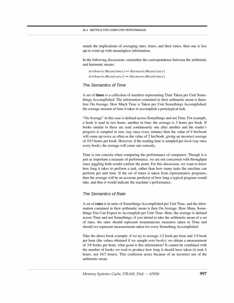
stands the implications of averaging rates, times, and their ratios, then one is lessapt to wind up with meaningless information.

In the following discussions, remember the correspondence between the arithmeticand harmonic means:

The Semantics of Time

A set of times is a collection of numbers representing Time Taken per Unit Some-things Accomplished. The information contained in their arithmetic mean is there-fore On Average, How Much Time is Taken per Unit Somethings Accomplished;the average amount of time it takes to accomplish a prototypical task.

“On Average” in this case is defined across Somethings and not Time. For example,a book is read in two hours, another in four; the average is 3 hours per book. Ifbooks similar to these are read continuously one after another and the reader’sprogress is sampled in time (say once every minute) then the value of 4 hrs/bookwill come up twice as often as the value of 2 hrs/book, giving an incorrect averageof 10/3 hours per book. However, if the reading time is sampled per book (say onceevery book), the average will come out correctly.

Time is our concern when comparing the performance of computers. Though it isjust as important a measure of performance, we are not concerned with throughputsince juggling both would confuse the point. For this discussion, we want to knowhow long it takes to perform a task, rather than how many tasks the machine canperform per unit time. If the set of times is taken from representative programs,then the average will be an accurate predictor of how long a typical program wouldtake, and thus it would indicate the machine’s performance.

The Semantics of Rate

A set of rates is in units of Somethings Accomplished per Unit Time, and the infor-mation contained in their arithmetic mean is then On Average, How Many Some-things You Can Expect to Accomplish per Unit Time. Here, the average is definedacross Time and not Somethings; if you intend to take the arithmetic mean of a setof rates, the rates should represent instantaneous measures taken in Time andshould not represent measurements taken for every Something Accomplished.

Take the above book example; if we try to average 1/2 book per hour and 1/4 bookper hour (the values obtained if we sample over books), we obtain a measurementof 3/8 books per hour; what good is this information? It cannot be combined withthe number of books we read to produce how long it should have taken (it took 6hours, not 16/3 hours). This confusion arises because of an incorrect use of thearithmetic mean.

ArithmeticMean times( ) HarmonicMean rates( )↔

ArithmeticMean rates( ) HarmonicMean times( )↔



When measuring computers, we are generally presented with a set of values takenper task completed—a set of benchmark results, each of which is the time taken toperform one of several tests—not a set of instantaneous measurements of progress,sampled every unit of time. Therefore, in general, finding the arithmetic mean of aset of rates is not a good idea, as it will lead to erroneous and misleading results.Use the harmonic mean of the execution times instead.

The Semantics of Ratios

Computer performance is often represented by a ratio of rates or times. It is a unit-less number, and when the reference time is in the numerator (as in a ratio of rates)the measurement means how much “faster” one thing is than another. When the ref-erence time is in the denominator (as in a ratio of times) the measurement meanswhat fraction of time the machine in question takes to perform a task, relative to thereference machine.

What does it mean to average a set of unitless ratios? The arithmetic mean of a setof ratios is a weighted average where the weights happen to be the running times ofthe reference machine. What information is contained in this value? If the referencetimes are thought of as the expected amount of time for each benchmark, theweighting might ensure that no benchmark result counts more than any other, andthe arithmetic mean would then represent what proportion of the expected time theaverage benchmark takes.

30.4.2 Problems with Normalization

Problems arise if we take the average of a set of normalized numbers. The follow-ing examples demonstrate the errors that occur. The first example compares theperformance of two machines, using a third as a benchmark. The second exampleextends the first to show the error in using averaged CPI values to compare perfor-mance. The third example is a revisitation of a recent proposal on this very topic.

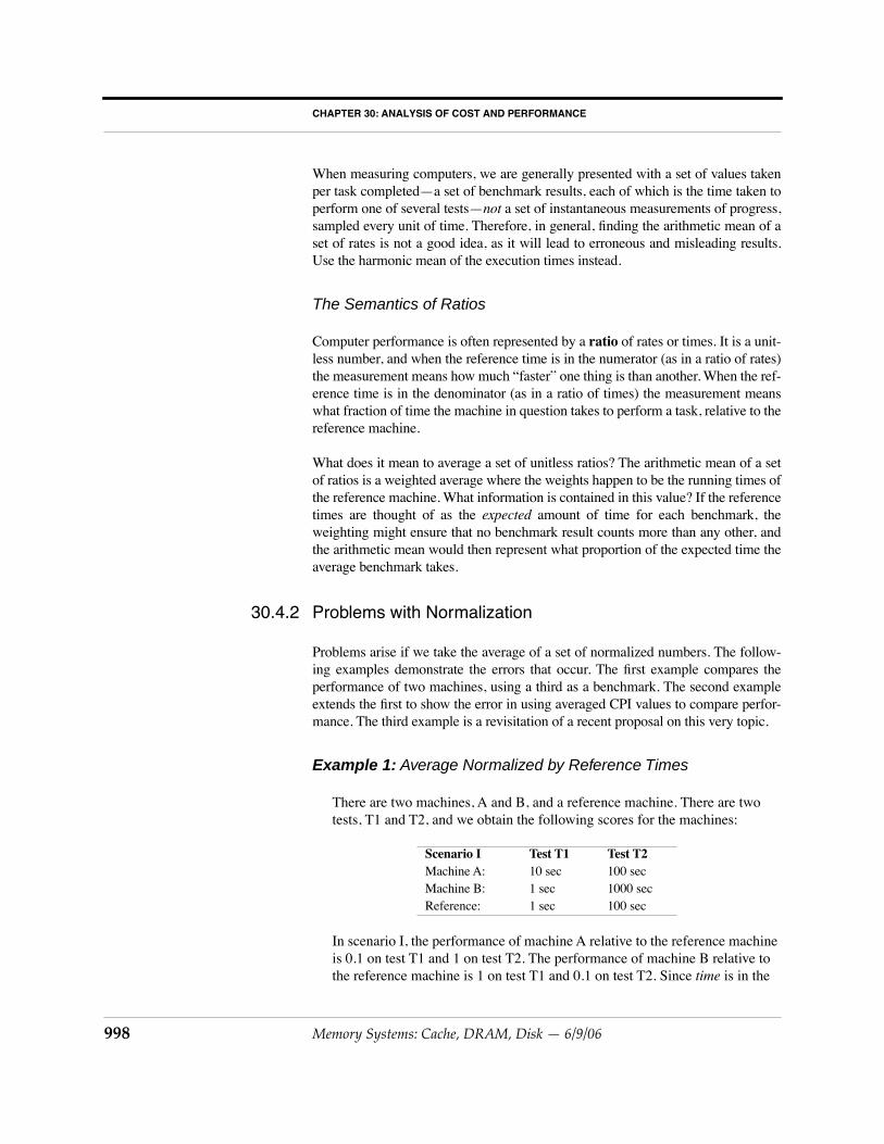
Example 1: Average Normalized by Reference Times

There are two machines, A and B, and a reference machine. There are two tests, T1 and T2, and we obtain the following scores for the machines:

In scenario I, the performance of machine A relative to the reference machine is 0.1 on test T1 and 1 on test T2. The performance of machine B relative to the reference machine is 1 on test T1 and 0.1 on test T2. Since time is in the

Scenario I Test T1 Test T2Machine A: 10 sec 100 secMachine B: 1 sec 1000 secReference: 1 sec 100 sec



denominator (the reference is in the numerator), we are averaging rates, there-fore we use the harmonic mean. The fact that the reference value is also in units of time is irrelevant; the time measurement we are concerned with is in the denominator, thus we are averaging rates.

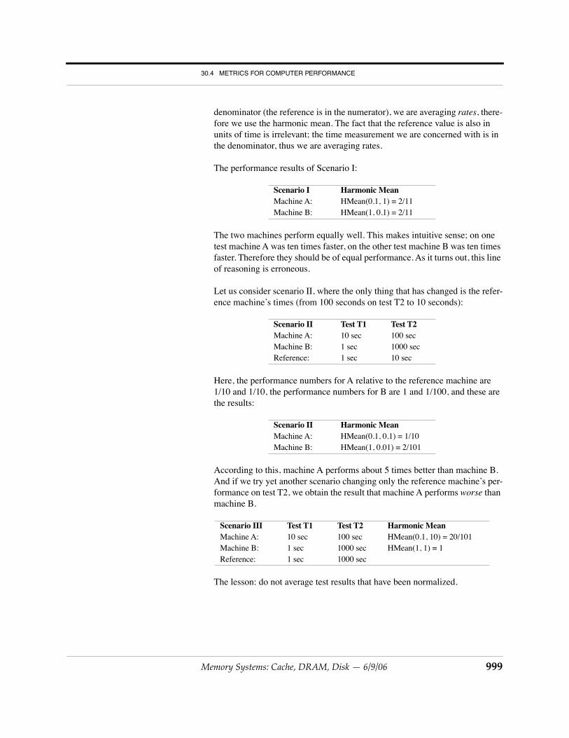
The performance results of Scenario I:

The two machines perform equally well. This makes intuitive sense; on one test machine A was ten times faster, on the other test machine B was ten times faster. Therefore they should be of equal performance. As it turns out, this line of reasoning is erroneous.

Let us consider scenario II, where the only thing that has changed is the refer-ence machine’s times (from 100 seconds on test T2 to 10 seconds):

Here, the performance numbers for A relative to the reference machine are 1/10 and 1/10, the performance numbers for B are 1 and 1/100, and these are the results:

According to this, machine A performs about 5 times better than machine B. And if we try yet another scenario changing only the reference machine’s per-formance on test T2, we obtain the result that machine A performs worse than machine B.

The lesson: do not average test results that have been normalized.

Scenario I Harmonic MeanMachine A: HMean(0.1, 1) = 2/11Machine B: HMean(1, 0.1) = 2/11

Scenario II Test T1 Test T2Machine A: 10 sec 100 secMachine B: 1 sec 1000 secReference: 1 sec 10 sec

Scenario II Harmonic MeanMachine A: HMean(0.1, 0.1) = 1/10Machine B: HMean(1, 0.01) = 2/101

Scenario III Test T1 Test T2 Harmonic MeanMachine A: 10 sec 100 sec HMean(0.1, 10) = 20/101Machine B: 1 sec 1000 sec HMean(1, 1) = 1Reference: 1 sec 1000 sec



Example 2: Average Normalized by Number of Operations

The example extends even further; what if the numbers were not a set of nor-malized running times but CPI measurements? Taking the average of a set of CPI values should not be susceptible to this kind of error, because the num-bers are not unitless; they are not the ratio of the running times of two arbi-trary machines.

Let us test this theory. Let us take the average of a set of CPI values, in three scenarios. The units are cycles per instruction, and since the time-related por-tion (cycles) is in the numerator, we will be able to use the arithmetic mean.

The following are the three scenarios, where the only difference between each scenario is the number of instructions performed in Test2. The running times for each machine on each test do not change, therefore we should expect the performance of each machine relative to the other to remain the same.

However, we obtain the anomalous result that the machines have different rel-ative performances which depend upon the number of instructions that were executed.

The theory is flawed. Average CPI values are not valid measures of computer performance. Taking the average of a set of CPI values is not inherently wrong, but the result cannot be used to compare performance. The erroneous behavior is due to normalizing the values before averaging them. If instead we average the running times before normalization, we get a value of 55 cycles for Machine A, and a value of 500.5 cycles for Machine B. This alone is the valid comparison. Again, this example is not meant to imply that average CPI values are meaningless, they are simply meaningless when used to compare the performance of machines.

Scenario I Test1 Test2 Arithmetic MeanMachine A: 10 cycles 100 cycles AMean(10, 10) = 10 CPIMachine B: 1 cycle 1000 cycles AMean(1, 100) = 50.5 CPIInstructions: 1 instr 10 instr Result: Machine A faster

Scenario II Test1 Test2 Arithmetic MeanMachine A: 10 cycles 100 cycles AMean(10, 1) = 5.5 CPIMachine B: 1 cycle 1000 cycles AMean(1, 10) = 5.5 CPIInstructions: 1 instr 100 instr Result: Equal performance

Scenario III Test1 Test2 Arithmetic MeanMachine A: 10 cycles 100 cycles AMean(10, 0.1) = 5.05 CPIMachine B: 1 cycle 1000 cycles AMean(1, 1) = 1 CPIInstructions: 1 instr 1000 instr Result: Machine B faster



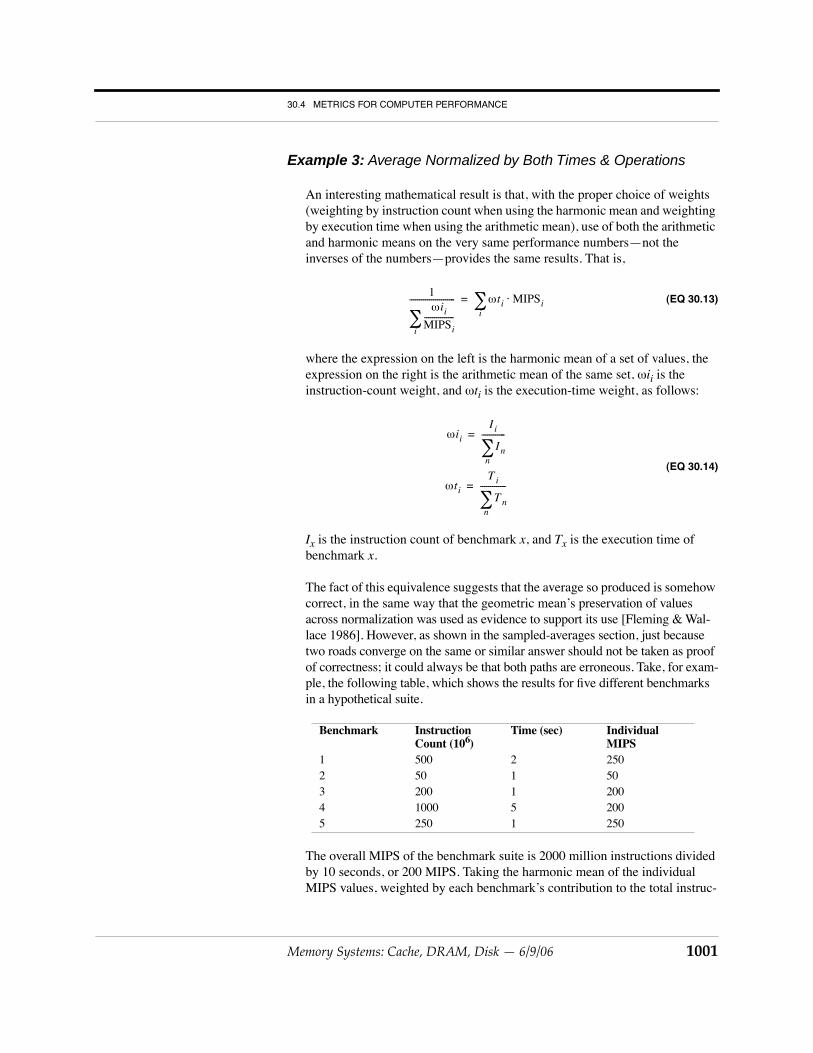
Example 3: Average Normalized by Both Times & Operations

An interesting mathematical result is that, with the proper choice of weights (weighting by instruction count when using the harmonic mean and weighting by execution time when using the arithmetic mean), use of both the arithmetic and harmonic means on the very same performance numbers—not the inverses of the numbers—provides the same results. That is,

(EQ 30.13)

where the expression on the left is the harmonic mean of a set of values, the expression on the right is the arithmetic mean of the same set, ωii is the instruction-count weight, and ωti is the execution-time weight, as follows:

(EQ 30.14)

Ix is the instruction count of benchmark x, and Tx is the execution time of benchmark x.

The fact of this equivalence suggests that the average so produced is somehow correct, in the same way that the geometric mean’s preservation of values across normalization was used as evidence to support its use [Fleming & Wal-lace 1986]. However, as shown in the sampled-averages section, just because two roads converge on the same or similar answer should not be taken as proof of correctness; it could always be that both paths are erroneous. Take, for exam-ple, the following table, which shows the results for five different benchmarks in a hypothetical suite.

The overall MIPS of the benchmark suite is 2000 million instructions divided by 10 seconds, or 200 MIPS. Taking the harmonic mean of the individual MIPS values, weighted by each benchmark’s contribution to the total instruc-

Benchmark Instruction Count (106)

Time (sec) Individual MIPS

1 500 2 2502 50 1 503 200 1 2004 1000 5 2005 250 1 250

1ωii

MIPSi---------------

i∑----------------------- ωti MIPSi⋅

i∑=

ωii

I i

Inn∑------------=

ωti

T i

T nn∑-------------=



tion count, yields an average of 200 MIPS. Taking the arithmetic mean of the individual MIPS values, weighted by each benchmark’s contribution to the total execution time, yields an average of 200 MIPS. This would seem to be a home run.

However, let’s skew the results by changing benchmark #2 so that its instruc-tion count is 200 times larger than before, and its execution time is also 200 times larger than before. The table now looks like this:

This is the same affect as looping benchmark #2 two hundred times. However, the total MIPS now becomes roughly 12000 million instructions divided by roughly 200 seconds, or roughly 60 MIPS. Thus, though this mechanism is very convincing, it is as easily spoofed as other mechanisms: the problem comes from trying to take the average of normalized values and interpret it to mean “performance.”

30.4.3 The Meaning of Performance

We have determined that the arithmetic mean is appropriate for averaging times(which implies that the harmonic mean is appropriate for averaging rates), and thatnormalization, if performed, should be carried out after the averaging. The questionarises: what does this mean?

When we say that the following describes the performance of a machine basedupon the running of a number of standardized tests (which is the ratio of the arith-metic means, with the constant N terms cancelling out),

(EQ 30.15)

then we implicitly believe that every test counts equally, in that on average it is usedthe same number of times as all other tests. This means that tests which are muchlonger than others will count more in the results.

Benchmark Instruction Count (106)

Time (sec) Individual MIPS

1 500 2 2502 10,000 200 503 200 1 2004 1000 5 2005 250 1 250

OurTimeii

N

∑

RefTime jj

N

∑--------------------------------



Perspective: Performance is Time Saved

We wish to be able to say, “this machine is X times faster than that machine.”Ambiguity arises because we are often unclear on the concept of performance.What do we mean when we talk about the performance of a machine? Why do wewish to be able to say this machine is X times faster than that machine? The reasonis that we have been using that machine (machine A) for some time and wish toknow how much time we would save by using this machine (machine B) instead.

How can we measure this? First, we find out what programs we tend to run onmachine A. These programs (or ones similar to them) will be used as the bench-mark suite to run on machine B. Next, we measure how often we tend to use theprograms. These values will be used as weights in computing the average (pro-grams used more should count more), but the problem is that it is not clear whetherwe should use values in units of time or number of occurrences; do we count eachprogram the number of times per day it is used or the number of hours per day it isused?

We have an idea about how often we use programs; for instance, every time we edita source file we might recompile. So we would assign equal weights to the wordprocessing benchmark and the compiler benchmark. We might run a different set of3 or 4 n-body simulations every time we recompiled the simulator; we would thenweight the simulator benchmark 3 or 4 times as heavily as the compiler and texteditor. Of course, it is not quite as simple as this, but you get the point; we tend toknow how often we use a program, independent of how slowly or quickly themachine we use performs it.

What does this buy us? Say for the moment that we consider all benchmarks in thesuite equally important (we use each as often as the other); all we need to do is totalup the times it took the new machine to perform the tests, total up the times it tookthe reference machine to perform the tests, and compare the two results.

It does not matter if one test takes three minutes and another takes three days—ifthe reference machine performs the short test in less than a second (indicating thatyour new machine is extremely slow) and it performs the long test in three days andsix hours (indicating that your new machine is marginally faster than the old one),the time saved is about six hours. Even if you use the short program a hundredtimes as often as the long program, the time saved is still an hour over the oldmachine.

The error is that we considered performance to be a value which can be averaged;the problem is our perception that performance is a simple number. The reason forthe problem is that we often forget the difference between the following statements:

• on average, the amount of time saved by using machine A over machine B is …

• on average, the relative performance of machine A to machine B is …



Rethinking Metrics for Performance

We usually know what we need to do; we are interested in how much of it we canget done with this computer versus that one. In this context, the only thing that mat-ters is how much time is saved by using one machine over another. The fallacy is inconsidering performance a measure unto itself. Performance is in reality a specificinstance of the following:

• two machines,

• a set of programs to be run on them,

• and an indication of how important each of the programs is to us.

Performance is therefore not a single number, but really a collection of implica-tions. It is nothing more or less than the measure of how much time we save run-ning our tests on the machines in question. If someone else has similar needs toours, our performance numbers will be useful to them. However, two people withdifferent sets of criteria will likely walk away with two completely different perfor-mance numbers for the same machine.

Rules to Live By

1. When presented with a number of times for a set of benchmarks, the appropri-ate average is the arithmetic mean.

2. When presented with a number of rate ratios for a set of benchmarks (refer-ence time over experimental time, such as in SPECmarks), sum the individual running times and use the ratio of the sums (equivalent to the ratio of the arith-metic means).

3. When presented with a number of time ratios for a set of benchmarks (experi-mental time over reference time), sum the individual running times and use the ratio of the sums (equivalent to the ratio of the arithmetic means).

4. When presented with a set of rates, the harmonic mean is appropriate.

30.5 Analytical Modeling and the Miss-Rate Function

The classical cache miss-rate function, as defined by Stone, Smith, and others, isM(x) = βxα for constants β and negative α and variable cache size x [Smith 1982,Stone 1993]. This function has been shown to accurately describe the shape of thecache miss rate as a function of cache size. However, this function, when useddirectly in optimization analysis without any alterations to accommodate boundary


30.5 ANALYTICAL MODELING AND THE MISS-RATE FUNCTION

cases, can lead to erroneous results. This section presents the mathematical insightbehind the behavior of the function under the Lagrange multiplier optimizationprocedure and shows how a simple modification to the form solves the inherentproblems.

30.5.1 Analytical Modeling

Numerous articles have been written about memory hierarchies*, generally focus-ing on a two-level hierarchy. Most studies after 1980 used trace- and execution-driven simulation to investigate such aspects of cache performance as multiproces-sor cache coherence and replacement strategies. Benchmark-specific simulationstudies are valuable for understanding cache behavior on particular workloads, butthey are not easily applied to other workloads [Smith 1982].

Unlike execution traces, mathematical analysis lends itself well to understandingcache behavior on general workloads, though such generality usually leads to lessaccurate results. Many researchers have used such analysis on memory hierarchiesin the past. Chow showed that the optimum number of cache levels scales with thelogarithm of the capacity of the cache hierarchy [Chow 1974, 1976]. Garcia-Molina and Rege demonstrated that it is often better to have more of a slowerdevice than less of a faster device [Garcia-Molina et al. 1987, Rege 1976]. Welchshowed that the optimal speed of each level must be proportional to the amount oftime spent servicing requests out of that level [Welch 1978].

A more recent mathematical analysis [Jacob et al. 1996] complements this earlierwork and provides intuitive understanding of how budget and technology charac-teristics interact. The analysis is the first to find a closed-form solution for the sizeof each level in a general memory hierarchy, given device parameters (cost andspeed), available system budget, and a measure of the workload’s temporal locality.The model recommends cache sizes that surprise many people (including theauthors). In particular, with little money to spend on the hierarchy, the model rec-ommends spending it all on the cheapest, slowest storage technology rather thanthe fastest. This is contrary to the common practice of focusing on satisfying asmany references in the fastest cache level, such as the L1 cache for processors orthe file cache for storage systems. Interestingly, it does reflect what has happened inthe PC market, where processor caches have been among the last levels of thememory hierarchy to be added.

The model provides intuitive understanding of memory hierarchies and indicateshow one should spend one’s money. Figure 30.7 pictures examples of optimal allo-cations of funds across 3- and 4-level hierarchies (e.g. several levels of cache,DRAM, and/or disk). The costs and access times for the technologies in the hierar-

* Articles by A. J. Smith [Smith 1982, Smith 1985] provide excellent overviews of CPU and disk caches.



chy are constants and need only be “realistic” values: costs should monotonicallydecrease and access times should monotonically increase as one moves down thehierarchy (to a larger i). The figures are applicable across all choices of technolo-gies for the cache hierarchy using realistic values for costs and access times.

In general, the first dollar spent by a memory-hierarchy designer should go to thelowest level in the hierarchy. As money is added to the system, the size of this levelshould increase, until it becomes cost-effective to purchase some of the next levelup. From that point on, every dollar spent on the system should be divided betweenthe two levels in a fixed proportion, with more bytes being added to the lower levelthan the higher level. This does not necessarily mean that more money is spent onthe lower level. Every dollar is split this way until it becomes cost-effective to addanother hierarchy level on top, and from that point on every dollar is split threeways, with more bytes being added to the lower levels than the higher levels, until itbecomes cost-effective to add another level on top. Since real technologies do notcome in arbitrary sizes, hierarchy levels will increase as step functions approximat-ing the slopes of straight lines.

The interested reader is referred to the article for more detail and analysis.

30.5.2 The Miss-Rate Function

As mentioned, there are many analytical cache papers in the literature, and many ofthese use the classical miss-rate function M(x) = βxα. This function is a direct out-

X_2 X_1System Budget

Siz

e of

Lev

el

Size of L3 CacheSize of L2 CacheSize of L1 Cache

X_1X_3 X_2System Budget

Siz

e of

Lev

el

Size of L4 CacheSize of L3 CacheSize of L2 CacheSize of L1 Cache

FIGURE 30.7: An Example of Solutions for Two Larger Hierarchies. A three-level hierarchy is shown on the left; a four-level hierarchy is shown on the right. Between inflection points (at which it is most cost-effective to add another level to thehierarchy) the equations are linear; the curves simply change slopes at the inflection points to adjust for the additional costof a new level in the hierarchy.



growth of the 30% Rule*, which states that successive doublings of cache sizeshould reduce miss rate by approximately 30%.

The function accurately describes the shape of the miss-rate curve, which repre-sents miss rate as a function of cache size, but it does not accurately reflect the val-ues at boundary points. Therefore the form cannot be used in any mathematicalanalysis that depends on accurate values at these points. For instance, using thisform yields an infinite miss rate for a cache of size zero, whereas probabilitiesreside in the [0,1] range. Caches of size less than one will have arbitrarily largemiss rates (greater than unity). While this is not a problem when one is simplyinterested in the shape of a curve, it can lead to significant errors if one uses theform in optimization analysis, in particular the technique of Lagrange multipliers.This has lead some previous analytical cache studies to reach half-completed solu-tions or (in several cases) outright erroneous solutions.

The classical miss-rate function can be used without problem provided that its formbehaves well, i.e. it must return values between 1 and 0 for all physically realizable(non-negative) cache sizes. This requires a simple modification; the original func-tion M(x) = βxα becomes M(x) = (βx + 1)α. The difference in form is slight, yet thedifference in results and conclusions that can be drawn are very large. The classicalform suggests that the ratio of sizes in a cache hierarchy is a constant; if onechooses a number of levels for the cache hierarchy, then all levels are present in theoptimal cache hierarchy. Even at very small budget points, the form suggests thatone should add money to every level in the hierarchy, in a fixed proportion deter-mined by the optimization procedure.

By contrast, when one uses the form M(x) = (βx + 1)α for the miss-rate function,one reaches the conclusion that the ratio of sizes in the optimal cache hierarchy isnot constant; in fact, at small budget points, certain levels in the hierarchy shouldnot appear. At very small budget points, it does not make sense to appropriate one’sdollar across every level in the hierarchy; it is better spent on a single level in thehierarchy, until one has enough money to afford adding another level. This is theconclusion reached in [Jacob et al. 1996].

* The 30% Rule, first suggested by Smith [1982], is the rule of thumb that every dou-bling of a cache’s size should reduce the cache misses by 30%. Solving the recurrence relation

(EQ 30.1)

yields a polynomial of the form

(EQ 30.2)

where α is negative.

0.7 f x( ) f 2x( )=

f x( ) βxα

=



The form of the miss-rate function M(x), intuitive explanation

The technique of Lagrange multipliers may be used in situations that obey certainstipulations; the model does not support inequalities, and the functions involvedmust be differentiable at all points of interest. For instance, if the function M(x) =βxα is a staircase function, one cannot use it in Lagrange analysis.

First, assume that the miss-rate function has the form M(x) = βxα and is correct.Clearly, this violates the differentiability assertion, but there are other compellingreasons to find fault with the form. Note the β term: it is included in the functionbecause the problem is not mathematically restricted to any particular scale—val-ues for x can be in bytes, kilobytes, megabytes, petabytes, or even something oddlike 3.14159 bits. The analysis must therefore allow cache sizes below 1, else iteliminates from consideration a potentially large fraction of the solution space.

To continue, if the miss rate for a cache of size x is given by M(x) = βxα, what thenis the miss rate for a cache of size zero? What is the miss rate for a cache of size1/1024? If x is in units of megabytes, this is a very reasonable question. The formM(x) = βxα is perfectly content to return miss rates larger than unity when x is lessthan one. Clearly, this is a critical weakness of the form.

A simple solution replaces x by x+1, yielding M(x) = β(x+1)α. There are two prob-lems with this form, as with the form M(x) = βxα. The first is that, to make M(x)unitless, β must be in units that are dependent on α. This is not an enormous math-ematical dilemma (for example, one could argue that x, cache size, should be unit-less, which would solve the problem); nonetheless it is not particularly reassuring.A more important problem is that, depending on the value of β (e.g. if β is largerthan 1), this form can also yield miss rates greater than unity. Perhaps most impor-tantly, the form of the function does not guarantee the miss rate of a cache of sizezero to be unity; a cache of size zero will have a miss rate of β, not 1 (miss rate isonly unity if β is defined to be 1, which is not particularly useful). The problem isthat the function does not behave properly at the boundary cases.

A solution is to scale x directly by β so that x and β have identical (but inverted)units. Therefore the numerator of the miss-rate function will have a value of 1 andthe minimum value for the denominator will be 1 (therefore the miss rate must beequal to unity for x = 0 and less than unity for all x > 0). This gives us a well-behaved form for the miss-rate function:

(EQ 30.16)

This form behaves well for all realistic values of x, α, and β (meaning x ≥ 0, α ≤ 0,and β ≥ 0). For a cache of size zero, it yields a miss rate of 1. For any finite cachelarger than zero, it yields values between 0 and 1 (0 < M(x) < 1), and as the cacheapproaches infinite size, M(x) → 0.

M x( ) βx 1+( )α

=



The form of the miss-rate function M(x), mathematical explanation

Since the miss rate is a decreasing function (α is implicitly negative), we willinstead use a positive value for α in the following analysis to make the physicalimplications more easily seen and to simplify the mathematics. Also for simplifica-tion, we will use a form for the miss-rate function that divides x by β rather thanmultiplying x by β; the only difference is that β cannot be 0.

The average access time of a hierarchy can be shown as a summation of miss prob-abilities or a summation of integrals. Analysis using a summation of integrals canbe found elsewhere [Jacob et al. 1996]; this section will use the summation of missprobabilities:

(EQ 30.17)

where there are n levels in the hierarchy (plus backing store), si is the size/capacityof level i in the hierarchy, and ti is the access time of level i in the hierarchy. Con-sider both forms of the miss-rate function:

(EQ 30.18)

First, we show the access-time using M1 for the miss-rate.

(EQ 30.19)

Note first that this yields arbitrarily large access times as the sizes of the cache lev-els si approach zero. This is unrealistic; a true cache hierarchy would have a maxi-mum access time of t1 + t2 + t3 + ... + tn + tn+1 (one would reference L1, discoverthe item missing, reference L2, discover the item missing, reference L3, etc.).Therefore if we use the M(x) = βxα form for the miss-rate function, we reach theconclusion that hierarchies can be built with arbitrarily large access times.

Now we look at both access-time models using the second form for the miss-ratefunction, M(x) = 1/(x/β + 1)α.

(EQ 30.20)

By simple inspection one can see that it is impossible to have a hierarchy with aninfinite access time: if all si are zero (for i from 0 to n), we reach the natural conclu-

T x Mx si 1–( ) ti⋅i 1=

n 1+

∑= s0 0≡

M1 x( ) β

xα

------= M2 x( ) 1

xβ--- 1+⎝ ⎠⎛ ⎞ α---------------------=

T 1 1 t1⋅β

s1α

-------- t2⋅β

s2α

-------- t3⋅ … β

snα

-------- tn 1+⋅+ + + +=

T 2

t1

s0

β---- 1+⎝ ⎠⎛ ⎞

α-----------------------

t2

s1

β---- 1+⎝ ⎠⎛ ⎞

α-----------------------

t3

s2

β---- 1+⎝ ⎠⎛ ⎞

α----------------------- …

tn 1+

sn

β---- 1+⎝ ⎠⎛ ⎞

α-----------------------+ + + +=



sion that the access time T equals t1 + t2 + t3 + ... + tn + tn+1. Another nice thingabout this form is that we do not need to define a value for M(s0); we can simplyplug s0 into the miss-rate function directly without yielding disastrous results.

Since the values in the denominators are constrained to be greater than or equal to 1for cache sizes greater than or equal to zero, it is intuitively clear that one cannotcreate arbitrarily large access times as is the case with the previous miss-rate form.However, one can choose values for si that yield arbitrarily high values for T. Forinstance, we can choose the following for si :

(EQ 30.21)

This yields arbitrarily large values for T—a hierarchy that has an access time of Xtimes the slowest access time in the hierarchy (tn+1). Clearly, this is impossible inan actual system. However, note that since ti < tn+1 when i < n+1 this gives us si < 0,∀i (for X larger than 1) which is meaningful mathematically but not physically.

Recap

The use of the miss-rate form M(x) = βxα is erroneous. It yields impossibly largemiss rates (greater than unity) for small cache sizes and leads to inconsistent andunrealistic physical interpretations; therefore a form that constrains the miss rate tobehave properly should be used. We suggest the form M(x) = (βx + 1)α, alterna-tively M(x) = (x/β + 1)α, both of which are guaranteed to give miss-rate valuesbetween 1 and 0 for all physically meaningful values for x, α, and β. The only dif-ference between the two forms is that the second cannot handle cases where β = 0.

30.5.3 Interesting Side-Effect of Lagrange Analysis

Let us look further at the problem of not being able to specify inequalities whenusing Lagrange multipliers. We may not restrict the values of x to be non-negativeor even non-zero; this leads to interesting results.

For this section, we return to a summation of integrals. The probability of accessinglevel i is equal to the probability that the reference will miss in all the levels aboveit:

(EQ 30.22)

where p(x) is the probability density function, the differential of the cumulativeprobability graph 1-M(x). The average system time spent per reference accessinglevel i is thus the time to reference level i scaled by this probability:

si βti 1+

Xtn 1+---------------⎝ ⎠⎛ ⎞

1 α⁄1–=

p x( )dx

si 1–

∞

∫



(EQ 30.23)

and the total system time spent per reference is the sum of the times across all lev-els in the hierarchy:

(EQ 30.24)

The size of the bottom storage level n+1 does not appear in the equation, since thislevel is assumed to contain all data, so sn+1 is for all intents infinite. The time to ref-erence this level does appear, scaled by the miss rate of the lowest cache level. Aswe expect, backing store is only referenced on misses to the lowest cache level.

Fig 30.8 illustrates the behavior of the access time function T as affected by thehierarchy organization. The graph illustrates a two-level hierarchy and the x-axisrepresents the proportion of the budget spent on each level of the hierarchy.Towards the left represents more money spent on the L2 cache, toward the rightrepresents more money spent on the L1 cache. The curves represent constant bud-get values. The graph demonstrates the function’s reduced sensitivity to hierarchyconfiguration as the budget increases.

ti p x( )dx

si 1–

∞

∫

T t1 p x( )dx

s0

∞

∫ t2 p x( )dx

s1

∞

∫ t3 p x( )dx

s2

∞

∫ … tn 1+ p x( )dx

sn

∞

∫+ + + +=

FIGURE 30.8: Behavior and Sensitivity of the Access Time Function. This is an example of the access time for a two-level hier-archy, depending upon what proportion of money is spent on which level in the hierarchy. The curves represent constant budget val-ues. As the budget increases, the sensitivity to hierarchy configuration decreases.

0 20 40 60 80 100Percentage of Budget Spent on L1

10

100

1000

Pre

dict

ed A

vg A

cces

s T

ime

(log)



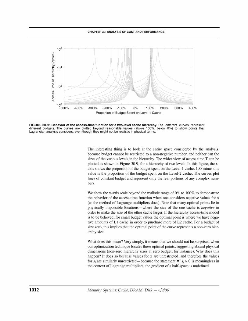
The interesting thing is to look at the entire space considered by the analysis,because budget cannot be restricted to a non-negative number, and neither can thesizes of the various levels in the hierarchy. The wider view of access time T can beplotted as shown in Figure 30.9, for a hierarchy of two levels. In this figure, the x-axis shows the proportion of the budget spent on the Level-1 cache. 100 minus thisvalue is the proportion of the budget spent on the Level-2 cache. The curves plotlines of constant budget and represent only the real portions of any complex num-bers.

We show the x-axis scale beyond the realistic range of 0% to 100% to demonstratethe behavior of the access-time function when one considers negative values for x(as the method of Lagrange multipliers does). Note that many optimal points lie inphysically impossible locations—where the size of the one cache is negative inorder to make the size of the other cache larger. If the hierarchy access-time modelis to be believed, for small budget values the optimal point is where we have nega-tive amounts of L1 cache in order to purchase more of L2 cache. For a budget ofsize zero, this implies that the optimal point of the curve represents a non-zero hier-archy size.

What does this mean? Very simply, it means that we should not be surprised whenour optimization technique locates these optimal points, suggesting absurd physicaldimensions (non-zero hierarchy sizes at zero budget, for instance). Why does thishappen? It does so because values for x are unrestricted, and therefore the valuesfor si are similarly unrestricted—because the statement ∀i si ≥ 0 is meaningless inthe context of Lagrange multipliers; the gradient of a half-space is undefined.

FIGURE 30.9: Behavior of the access-time function for a two-level cache hierarchy. The different curves representdifferent budgets. The curves are plotted beyond reasonable values (above 100%, below 0%) to show points thatLagrangian analysis considers, even though they might not be realistic in physical terms.

-500% -400% -300% -200% -100% 0% 100% 200% 300% 400%Proportion of Budget Spent on Level-1 Cache

100

102

104

106

Acc

ess-

Tim

e of

Hie

rarc

hy (

cycl

es)

Date post:	10-Mar-2020
Category:	Documents
Upload:	others
View:	25 times
Download:	0 times

Analysis of Cost and Performance - University Of...

Documents