Analysis of Environmental Data - UMass Amherst · Probability distributions 7 1.3 Probability...

Analysis of Environmental DataConceptual Foundations:Pro b ab ility Dis trib u tio n s

1. What is a probability (stochastic) distribution?. . . . . . . . . . . . . . . . . . . . . . . . . . . . . . . . . . . . . . 21.1 Measurement error versus process error. . . . . . . . . . . . . . . . . . . . . . . . . . . . . . . . . . . . . . . 31.2 Conventional versus hierarchical models. . . . . . . . . . . . . . . . . . . . . . . . . . . . . . . . . . . . . . 51.3 Probability distributions. . . . . . . . . . . . . . . . . . . . . . . . . . . . . . . . . . . . . . . . . . . . . . . . . . . . 6

2. Discrete distributions. . . . . . . . . . . . . . . . . . . . . . . . . . . . . . . . . . . . . . . . . . . . . . . . . . . . . . . . . . 72.1 Probability mass function.. . . . . . . . . . . . . . . . . . . . . . . . . . . . . . . . . . . . . . . . . . . . . . . . . 112.2 Cumulative probability distribution. . . . . . . . . . . . . . . . . . . . . . . . . . . . . . . . . . . . . . . . . . 122.3 Quantile distribution. . . . . . . . . . . . . . . . . . . . . . . . . . . . . . . . . . . . . . . . . . . . . . . . . . . . . 132.4 Random numbers. . . . . . . . . . . . . . . . . . . . . . . . . . . . . . . . . . . . . . . . . . . . . . . . . . . . . . . . 142.5 Binomial examples. . . . . . . . . . . . . . . . . . . . . . . . . . . . . . . . . . . . . . . . . . . . . . . . . . . . . . . 15

3. Continuous probability distributions. . . . . . . . . . . . . . . . . . . . . . . . . . . . . . . . . . . . . . . . . . . . . 163.1 Probability density function. . . . . . . . . . . . . . . . . . . . . . . . . . . . . . . . . . . . . . . . . . . . . . . . 193.2 Cumulative probability distribution. . . . . . . . . . . . . . . . . . . . . . . . . . . . . . . . . . . . . . . . . . 203.3 Quantile distribution. . . . . . . . . . . . . . . . . . . . . . . . . . . . . . . . . . . . . . . . . . . . . . . . . . . . . 213.4 Random numbers. . . . . . . . . . . . . . . . . . . . . . . . . . . . . . . . . . . . . . . . . . . . . . . . . . . . . . . . 223.5 Normal (Gaussian) examples. . . . . . . . . . . . . . . . . . . . . . . . . . . . . . . . . . . . . . . . . . . . . . . 23

4. Bestiary of probability distributions. . . . . . . . . . . . . . . . . . . . . . . . . . . . . . . . . . . . . . . . . . . . . 244.1 Discrete distributions. . . . . . . . . . . . . . . . . . . . . . . . . . . . . . . . . . . . . . . . . . . . . . . . . . . . . 254.2 Continuous distributions. . . . . . . . . . . . . . . . . . . . . . . . . . . . . . . . . . . . . . . . . . . . . . . . . . 29

5. Choosing the right probability distribution?. . . . . . . . . . . . . . . . . . . . . . . . . . . . . . . . . . . . . . . 376. Statistical Models – putting it all together. . . . . . . . . . . . . . . . . . . . . . . . . . . . . . . . . . . . . . . . . 38

Probability distributions 2

1. What is a probability (stochastic) distribution?

Recall that the deterministic part of the statistical model describes the expected pattern in theabsence of any kind of randomness or measurement error. The noise or error about the expectedpattern is the stochastic component of the model. To formally estimate the parameters of the model,you need to know not just the expected pattern (the deterministic component) but also somethingabout the variation about the expected pattern (the stochastic component). Typically, you describethe stochastic model by specifying a reasonable probability distribution for the variation about theexpected pattern (see below).


1.1 So u rc e s o f e rro r

The variation about the expected pattern, i.e., the stochastic component of the model, is oftentermed “noise”. Noise appears in environmental data in two different ways – as measurement error(sometimes called observation error) and as process noise – and it can be exacerbated by modelerror.

Briefly, measurement error is the variability or “noise” in our measurements having nothing to do withthe environmental system per se, only in our ability to accurately measure the system. Measurementerror makes it hard to estimate parameters and make inferences about environmental systems; morespecifically, it leads to large confidence intervals and low statistical power.


Even if we can eliminate measurement error (or make it trivially small), process noise or process error(often so-called even though it isn’t technically an error but a real part of the system) still existsbecause variability affects all environmental systems. For example, as Bolker (2008) describes, wecan observe thousands of individuals to determine the average mortality rate with great accuracy.The fate of a group of individuals, however, depends both on the variability in mortality rates ofindividuals and on the demographic stochasticity that determines whether a particular individuallives or dies. So even though we know the average mortality rate perfectly, our predictions are stilluncertain. Additionally, environmental stochasticity – spatial and temporal variability in e.g.mortality rate caused by variation in the environment rather than by the inherent randomness ofindividual fates – also affects the dynamics, introducing additional variability.


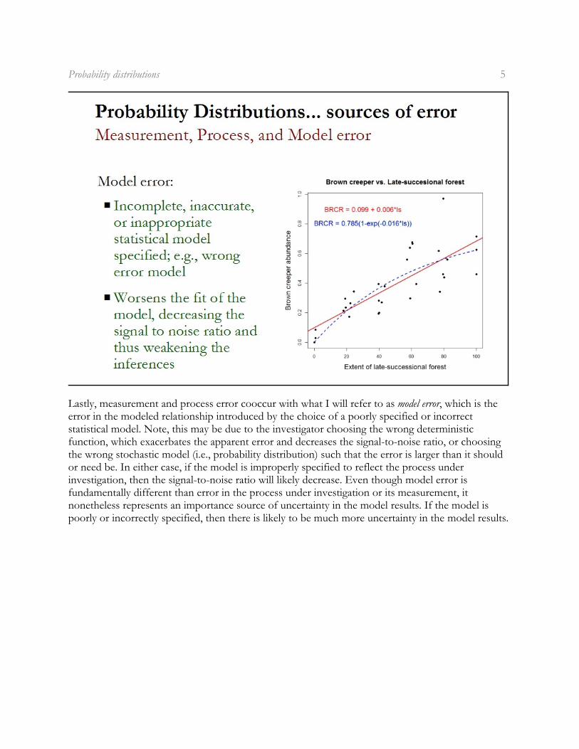
Lastly, measurement and process error cooccur with what I will refer to as model error, which is theerror in the modeled relationship introduced by the choice of a poorly specified or incorrectstatistical model. Note, this may be due to the investigator choosing the wrong deterministicfunction, which exacerbates the apparent error and decreases the signal-to-noise ratio, or choosingthe wrong stochastic model (i.e., probability distribution) such that the error is larger than it shouldor need be. In either case, if the model is improperly specified to reflect the process underinvestigation, then the signal-to-noise ratio will likely decrease. Even though model error isfundamentally different than error in the process under investigation or its measurement, itnonetheless represents an importance source of uncertainty in the model results. If the model ispoorly or incorrectly specified, then there is likely to be much more uncertainty in the model results.


1.2 Co n v e n tio n al v e rs u s h ie rarc h ic al m o d e ls

The distinction between measurement (or observation) and process error can be very important, andseparating these two sources of error is the basis for one whole class of multi-level or hierarchicalmodels (which we will discuss further in a later section). The example shown here was taken fromRoyle and Dorazio (2008) and was derived from the Swiss Survey of Common Breeding Birds. Thedata represent the presence/absence of the Willow Tit on 237 1 km quadrats in relation to two2

covariates that affect the species’ distribution: forest cover and elevation. A conventional (i.e.,nonhierarchical) logistic regression model was fit to the data in which the errors associated with thespecies occurrence on a plot (i.e., process error) and the error associated with detecting the speciesgiven it is present (i.e., measurement error) are confounded. A hierarchical model was also fit to thedata in which the two sources of error are modeled separately. The figures shown here depict thefitted response in occurrence probability for the willow tit to forest cover and elevation. The solidline and dotted lines show the fitted responses for the conventional and hierarchical models,respectively. Even though the general relationships are the same between models, the response toboth covariates is significantly stronger in the hierarchical model. In extreme cases, failure toseparately account for both observation and process error can lead to erroneous conclusions.


1.3 Pro b ab ility d is trib u tio n s

Formally, a probability distribution is the set of probabilities on a sample space or set of outcomes; itdescribes the set of probabilities for all possible outcomes of a random variable. Here, we will alwaysbe working with sample spaces that are numbers – the number or amount observed in somemeasurement of an environmental system. Importantly, the probability distribution deals with thetype (scale) of the dependent variable, not the independent variable(s). In the context of a statisticalmodel, it is perhaps easiest to think about a probability distribution as a description of the stochasticcomponent of the model, representing the random variability about the expected value (typically themean). In the simple linear regression example shown here, where the expected value of browncreeper abundance is a linear function of the extent of late-successional forest, the observed valuesof brown creeper abundance deviate from the expected (fitted) values in every case. Thesedifferences are the “errors” in the model (these errors are also called “residuals” as they representthe residual variability not accounted for by the deterministic model). The probability distributiondescribes the distribution of these errors, and is shown here as a histogram. Note, to fit this modelusing parametric methods, we had to assume that these errors were drawn from a specificdistribution (the normal distribution in this case) having one or more parameters that control itsshape, location and/or scale. The histogram reveals that this was a reasonable assumption in thiscase. Note that the assumption of a particular probability distribution is the basis for all so-calledparametric statistical methods. Lastly, it can be useful to think of the probability distribution as a sortof data-generating mechanism; an engine that randomly generates the data points that we ultimatelyobserve in our sample. This random data generating mechanism is necessary to simulate data, whichwe will discuss in a later section.


2. Discrete distributions

The simplest distributions to understand are discrete distributions whose outcomes are a set ofintegers; most of the discrete distributions we deal with describe counting or sampling processes andhave ranges that include some or all of the nonnegative integers. Note, discrete data generally arisefrom counting indivisible units. For example, a count of the number of individuals on a plot isdiscrete since individuals are indivisible – at least if they want to remain an individual. However,counting the basal area of trees on a plot (e.g., m /ha) but recording it to the nearest integer value2

doesn’t mean that basal area is discrete, only that your measurement precision is to the nearestinteger. Recording a continuous variable on a discrete scale doesn’t make the variable truly discrete,even if it allows you treat the data as if it were discrete – and thus use a discrete probabilitydistribution. However, there are occasional cases when it may make sense or even be necessary tomake your continuous data discrete for the analysis or, conversely, treat count data is if it werecontinuous, but in general it is probably best to remain faithful to the intrinsic scale of the variable.


As an example, one of the most common discrete distributions in environmental science and theeasiest to understand is the binomial. It applies when you have samples (observational units) with afixed number of subsamples or “trials” in each one, and each trial can have one of two values (e.g.,present/absent, alive/dead), and the probability of “success” (present, alive) is the same in everytrial. Consider the presence/absence of a focal species across 10 plots (subsamples) within a sample(observational) unit, say a watershed. At each plot, the species is either “present” or “absent”, whichwe usually represent as a 1 and a 0, respectively. If we survey all 10 plots (trial size=10) within eachsample and the probability of the species being present is prob=0.3, then the probability of observingthe species present at say 4 plots (k=4) within a sample will have a binomial distribution withparameters size=10 and prob=0.3. What type of data does this example represent?

Hopefully you answered proportional, since each sample (observational) unit has a fixed number oftrials, each of which can take on a binary response, such that the number of successes can beexpressed as a proportional of the total number of trials (e.g., 3 out 10). What if each sample unithad only a single trial (i.e., size=1). What kind of data would this be? Hopefully you answered binary,since each sample unit can take on only one of two values (e.g., present or absent, success or failure).The key here is to note that binary data is just the special case of proportional data when the trialsize equals 1. As a result, the binomial distribution is appropriate for both data types.


The easiest way to think about this is as follows. For a single sample consisting of 10 plots, we willobserve the species to be present a certain number of times, right? The range of possibilities is 0-10,since there are 10 plots – this constitutes the full set of possible outcomes. If the probability of thespecies being present on any single plot is prob=0.3, then on average we should expect to observethe species on 3/10 plots. However, given random variability in the environmental system (and theerror in our ability to accurately detect the species), it is quite possible that for any given randomsample of 10 plots, we might easily observe the species present on say only 1 or 2 plots or perhaps 4or 5 plots, but it seems highly unlikely that we would observe the species present on all 10 plots.Numerically, we can figure out the likelihood of the species being present 0, 1, ... 10 times bydrawing repeated samples, each time recording the number of presences across the 10 plots (k).After we draw a large number of samples, we can plot the distribution of k.


The frequency of samples with any particular value of k can be converted into a probability simplyby dividing it by the total number of samples in the distribution (or the cumulative area of thefrequency distribution). If we plot the result, we have the empirical probability distribution (given aspecial name below) which depicts the probability of observing any particular value of k. Of course,the empirical probability distribution shown here is specific to this data set; it gives the actualprobability that we observed each value of k (# successes) in this dataset. However, we typicallywant to know the theoretical probability distribution; the probability of observing each value of kfrom an infinitely large sample, under the assumption that our sample was drawn from such adistribution. Of course we don’t have to actual collect hundreds or thousands of samples in order tocalculate the approximate theoretical probability distribution, since the mathematical properties ofthe binomial distribution (and many others, see below) are known.


2.1 Pro b ab ility m as s fu n c tio n

For a discrete distribution, the probability distribution (often referred to as the probability mass functionor pmf for short) represents the probability that the outcome of an experiment or observation (calleda random variable) X is equal to a particular value x (f(x)=Prob(X=x)). In the case of the binomialdistribution, for example, we can calculate the probability of any specified number of successes (x=k)given the number of trials (size or N) and the probability of success (prob or just p) for each trial. Inthe example shown here, the probability of the species being present at 4 of the 10 plots given a pertrial probability of success prob=0.3 is 0.2.


2.2 Cum u lativ e p ro b ab ility d is trib u tio n

The cumulative probability distribution represents the probability that a random variable X is lessthan or equal to a particular value of x (f(x)=Prob(X#x)). Cumulative distribution functions aremost useful for frequentist calculations of so-called tail probabilities, or p-values. In the case of thebinomial distribution, for example, we can calculate the probability of the species being present k orfewer times given the number of trials (size) and the probability of success (prob) for each trial. In theexample shown here, the probability of the species being present at 4 or fewer plots out of 10 givena per trial probability of success prob=0.3 is 0.85. Thus, if we were to repeatedly draw samples of 10(trials) given a per trial probability of success prob=0.3, then we would expect to observe the speciespresent on 4 or fewer plots 85% of the time. Conversely, then, we would expect to observe thespecies present on 5 or more plots 15% of the time. Thus, the probability of observing the speciespresent on 5 or more plots if the sample was drawn from a binomial distribution with size=10 andprob=0.3 would be 0.15, or p=015. We refer to this as the “tail” probability because it represents theprobability of being in the tail of the probability distribution; the probability of being 5 or greater inthis case. We also call this the p-value, which is the standard basis for hypothesis testing, which wewill return to later.


2.3 Quan tile d is trib u tio n

The quantile distribution represents the value of x for any given quantile (proportion) of thecumulative probability distribution; i.e., it is the opposite of the cumulative probability distribution.In the case of the binomial distribution, for example, we can calculate the number of times thespecies is expected to be present k or fewer times for any specified probability level given thenumber of trials (size) and the per trial probability of success (p). In the example shown here, thespecies is expected to present on 5 or fewer plots out of 10 in 90 out of every 100 samples given aper trial probability of success prob=0.3.


2.4 Rand o m num b e rs

Random numbers can be drawn from a specified probability distribution. For example, in thebinomial example shown here, we can draw a random sample from the specified binomialdistribution (i.e., given trial size and per trial probability of success). The result is the number ofsuccesses (or species’ presences, in this case) in a single sample of size=10 given a per trialprobability of success prob=0.3. Note, if we repeat this process, we would expect to observe adifferent result each time owing to chance. Indeed, it is this variability that gives rise to theprobability distribution.


2.5 B in o m ial e xam p le s

There are lots of examples of data well suited to the binomial distribution:

• # adult female salamanders that successfully breed in a pond (observational unit). In thisexample, the pond is the sample (observational) unit, the # females attempting to breed is thetrial size, and the # successful females is the outcome of the set of trials (breeding attempts).The proportion of breeding females that are successful is distributed binomially. Note, in thiscase, if multiple ponds are sampled, the trial size is likely to vary among ponds – this is OK withproportional data.

• # point intercepts along a transect or grid that intersect a focal plant species out of a total # ofpoint intercepts taken on a vegetation plot. In this example, the vegetation plot is the sample(observational) unit, the # of point intercepts taken is the trial size, and the # of point interceptsintersecting the focal plant species is the outcome of the set of trials (point intercepts). Theproportional cover of the focal plant species is distributed binomially. Note, in this case, inmultiple vegetation plots are sampled, the trial size is likely to be fixed by study design.

• Can you think of other examples of either proportional data or binary data where the trial size is1?


3. Continuous probability distributions

A probability distribution over a continuous range (such as all real numbers, or the nonnegative realnumbers) is called a continuous distribution.

As an example, the most common continuous distribution in ecology (and all of statistics) and theeasiest to understand is the normal.


The normal distributionapplies when you havesamples that can take onany real number and forwhich there is a centraltendency (usually describedby the mean). Consider thesize of fish in a particularstream. Each fish has a sizethat can take on anynonnegative real number(>0). If the size distributionof fish in the population issymmetric about the mean(ì) with a standarddeviation (sd) or spreadabout the mean equal to ó,then the probability ofobserving a fish of size y will have a normal distribution with parameters ì and ó.


Continuous probability distributions are a bit more confusing to understand than discretedistributions. Let’s consider the fish size example further. The frequency of fish of any particularsize (i.e., the frequency distribution, as shown) can’t be converted into a probability simply bydividing it by the total number of samples in the distribution (or the cumulative area of thefrequency distribution) as we did with the discrete distribution. This is because, unlike the discretedistribution, we can’t enumerate all possible outcomes of the continuous random variable because itcan take on any real number – at least theoretically. In the fish size example, you may imagine that ameasurement of size is exactly 7.9 cm, but in fact what you have observed is that the size is between7.85 and 7.95 cm – if your scale has a precision of ±0.1 cm. Thus, continuous probabilitydistributions are expressed as probability densities rather than probabilities – the probability thatrandom variable X is between x and x+ªx, divided by ªx (Prob(7.85 < X < 7.95)/0.1, in this case).Dividing by ªx allows the observed probability density to have a well-defined limit as precisionincreases and ªx shrinks to zero. Unlike probabilities, probability densities can be larger than 1. Inpractice, we are concerned mostly with relative probabilities or likelihoods, and so the maximumdensity values and whether they are greater than or less than 1 don’t matter much.


3.1 Pro b ab ility d e n s ity fu n c tio n

For a continuous distribution, the probability distribution is referred to as a probability density function(or pdf for short). In the case of the normal distribution, for example, we can calculate the probabilitydensity for any specified value of X given the mean (ì) and standard deviation (ó). In the exampleshown here, the probability density for an individual with size = 8 cm given an underlying mean ofsay 10 cm and a standard deviation of say 2 cm is 0.12.


3.2 Cum u lativ e p ro b ab ility d is trib u tio n

The cumulative probability distribution represents the probability that a random variable X is lessthan or equal to a particular value of x (f(x) = Prob(X#x)). Remember, cumulative distributionfunctions are most useful for frequentist calculations of tail probabilities. In the case of the normaldistribution, for example, we can calculate the probability of a fish being smaller than or equal to anygiven size given the mean fish size (ì) and the standard deviation (ó). In the example shown here, theprobability of a fish less than or equal to 8 cm given an underlying mean of 10 cm and sd of 2 cm is0.16.


3.3 Quan tile d is trib u tio n

The quantile distribution represents the value of x for any given quantile (proportion) of thecumulative probability distribution; i.e., it is the opposite of the cumulative probability distribution.In the case of the normal distribution, for example, we can calculate the upper size limit belowwhich any specified percentage of the distribution lies given the mean fish size (ì) and the standarddeviation (ó). In the example shown here, fish are expected to be smaller than 12.56 cm 90 percentof the time given an underlying mean of 10 cm and sd of 2 cm.


3.4 Rand o m num b e rs

Random numbers can be drawn from a specified probability distribution. For example, in thenormal distribution example shown here, we can draw a random sample from the specified normaldistribution (i.e., given the mean and sd). The result is the size (in this case) of a single fish drawn atrandom from a normal distribution with mean of 10 cm and sd of 2 cm. Note, if we repeat thisprocess, we would expect to observe a different result each time owing to chance. Indeed, it is thisvariability that gives rise to the probability distribution.


3.5 No rm al (Gau s s ian ) e xam p le s

There are lots of examples of data well suited to the normal distribution:

• Home range size (ha) of individuals in a population. The individual is the sample (observational)unit and home range size is the measured continuous response that is likely to roughlysymmetrically distributed about a central mean value.

• Basal area (m /ha) of white pine stands. The forest stand is the sample (observational) unit and2

basal area is the measured continuous response that is likely to be roughly symmetricallydistributed about a central mean value.

• Temperature (degrees Celsius) on December 21 over the past 100 years. The year or day ofst

December 21 is the sample (observational) unit and temperature is the measured continuousresponse that is likely to roughly symmetrically distributed about a central mean value.

• Can you think of other examples of continuous data where the normal distribution makes sense?


4. Bestiary of probability distributions

There are a large number of well-established probability distributions. Some of these, like thebinomial and normal distributions discussed above, are already quite familiar to ecologists. Indeed,the normal distribution should be familiar to everyone as it is the distribution underlying most of theclassical statistical methods that we learned in introductory statistics courses. However, it is veryimportant to understand that there are many other probability distributions for both discrete andcontinuous data that have widespread application to environmental data. Indeed, some of thesedistributions address the shortcomings or limitations of the normal distribution for environmentaldata. Of course, a detailed description of all of the available distributions is way beyond the scope ofthis course. Instead, here we will briefly review a small bestiary of distributions that are useful inenvironmental modeling (summarized from from Bolker 2008 and Crawley 2007, but do see thesereferences for a more complete description).


4.1 Dis c re te d is trib u tio n s

4.1.1 Binomial

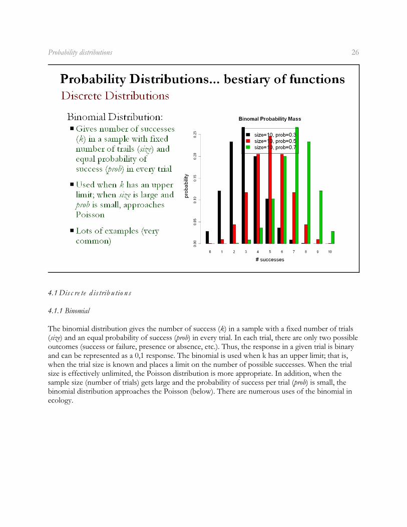
The binomial distribution gives the number of success (k) in a sample with a fixed number of trials(size) and an equal probability of success (prob) in every trial. In each trial, there are only two possibleoutcomes (success or failure, presence or absence, etc.). Thus, the response in a given trial is binaryand can be represented as a 0,1 response. The binomial is used when k has an upper limit; that is,when the trial size is known and places a limit on the number of possible successes. When the trialsize is effectively unlimited, the Poisson distribution is more appropriate. In addition, when thesample size (number of trials) gets large and the probability of success per trial (prob) is small, thebinomial distribution approaches the Poisson (below). There are numerous uses of the binomial inecology.


4.1.2 Poisson

The Poisson distribution gives the number of events in a given unit (space or time) of samplingeffort if each event is independent. The Poisson is used when you expect the number of events tobe effectively unlimited; if the number of events is limited, use the binomial distribution. ThePoisson is used only for count data; that is, events that can’t be meaningful divided into smaller unitssimply be changing the scale of the measurement (e.g., changing meters to centimeters). The Poissonis very common and familiar to ecologists because count data is so common to population andcommunity ecology.


4.1.3 Negative binomial

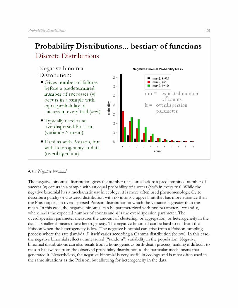
The negative binomial distribution gives the number of failures before a predetermined number ofsuccess (n) occurs in a sample with an equal probability of success (prob) in every trial. While thenegative binomial has a mechanistic use in ecology, it is more often used phenomenologically todescribe a patchy or clustered distribution with no intrinsic upper limit that has more variance thanthe Poisson; i.e., an overdispersed Poisson distribution in which the variance is greater than themean. In this case, the negative binomial can be parameterized with two parameters, mu and k,where mu is the expected number of counts and k is the overdispersion parameter. Theoverdispersion parameter measures the amount of clustering, or aggregation, or heterogeneity in thedata: a smaller k means more heterogeneity. The negative binomial can be hard to tell from thePoisson when the heterogeneity is low. The negative binomial can arise from a Poisson samplingprocess where the rate (lambda, ë) itself varies according a Gamma distribution (below). In this case,the negative binomial reflects unmeasured (“random”) variability in the population. Negativebinomial distributions can also result from a homogeneous birth-death process, making it difficult toreason backwards from the observed probability distribution to the particular mechanisms thatgenerated it. Nevertheless, the negative binomial is very useful in ecology and is most often used inthe same situations as the Poisson, but allowing for heterogeneity in the data.


4.1.4 Geometric

The geometric distribution has two closely related forms. One form gives the number of trials basedon the set {1, 2, ...} until you get a single success in a sample with equal probability of success (prob)in every trial. The alternative forms gives the number of failures based on the set {0, 1, 2, ...} untilyou get a single success in a sample with an equal probability of success (prob) in every trial. Note thesubtle differences between formulations. The probability mass distribution, along with the mean andvariance, are slightly different between forms. Note, the geometric is also a special case of thenegative binomial, with k =1. The geometric distribution is often used to describe survival time data,e.g., the number of successful/survived breeding seasons (i.e., interpreted as failures) for a seasonallyreproducing organism until it dies (i.e., interpreted as success), when time is considered as discreteunits (e.g., years). Alternatively, and more directly, it can be used to describe for example the numberof failed nesting attempts until the first success.


4.2 Co n tin u o u s d is trib u tio n s

4.2.1 Normal

The normal distribution is used everywhere and is the basis for most classical statistical methods. Itarises from the sum of many independent samples drawn from the same distribution (of any shape)and its ubiquity stems from the Central Limit Theorem, which says that if you add a large number ofindependent samples from the same distribution, the distribution of the sum will be approximatelynormal. The normal distribution has two parameters, the mean and standard deviation, which areindependent. Consequently, one often assumes constant variance (as the mean changes), in contrastto the Poisson and binomial distributions where the variance is a fixed function of the mean. Thenormal distribution is used with continuous, unimodal and symmetric distributions, which arereasonably common in ecology (e.g., temperature, pH, nutrient concentration).


4.2.2 Gamma

The Gamma distribution gives the distribution of waiting times until a certain number of events(shape) takes place, for example, the distribution of the length of time (in days) you would expect tohave to wait for 3 deaths in a population, given an average survival time. The Gamma distribution isthe continuous counterpart of the negative binomial, which recall is used to described anoverdispersed Poisson with heterogeneous data. The Gamma is similarly used in phenomenologicalfashion with continuous, positive data having too much variance and a right skew; in other words,an overdispersed normal distribution with a right skew. The Gamma is an excellent choice whenonly positive real numbers are possible (note the normal is not lower bounded like Gamma).


4.2.3 Exponential

The exponential distribution gives the distribution of waiting times for a single event to happengiven a constant probability per unit time (rate) that it will happen. The exponential is the continuouscounterpart of the geometric and is a special case of the Gamma with shape = 1. The exponential isused mechanistically when the distribution arises via waiting times, but it is also frequently usedphenomenologically for any continuous distribution that has highest probability for zero or smallvalues.


4.2.4 Beta

The beta distribution is closely related to the binomial; it gives the distribution of the probability ofsuccess in a binomial trial with a-1 observed successes and b-1 observed failures. It is the onlycontinuous probability distribution, besides the uniform, with a finite range, from 0 to 1. This makesit very useful when you have to define any continuous distribution on a finite range. The betadistribution is used with data in the form of probabilities or proportions (e.g., proportional cover).


4.2.5 Lognormal

The lognormal gives the distribution of the product of independent variables with the samedistribution, much like the normal except it stems from the product instead of a sum. The bestexample of this mechanism is the distribution of the sizes of individuals or populations that growexponentially, with a per capita growth rate that varies randomly over time. At each time step (e.g.,daily, yearly), the current size is multiplied by the randomly chosen growth increment, so the final size(when measured) is the product of the initial size and all of the random growth increments. Theeasiest way of thinking about the lognormal is that taking the log of a lognormal variable converts itto a normal variable. The lognormal is often used phenomenologically in situations when theGamma also fits.


4.2.6 Chi-square

The chi-square distribution gives the sum of squares of n (degrees of freedom) normals each withvariance one. The chi-square distribution is famous for its use in contingency table analysis (cross-classified categorical data) and the analysis of count data. For example, in a table of cross-classifiedcounts (males versus females and present versus absent), the Pearson’s chi-squared statistic is equalto the sum of the squared deviations between observed counts and expected counts divided byexpected counts, where expected counts are typically under the null hypothesis of independenceamong factors (sex and presence in this case). The chi-square is also especially important to usbecause Likelihood ratio statistics (which we will discuss in a later chapter), which are used to testfor the difference between nested models, are also approximately distributed chi-squared.


4.2.7 Fisher’s F

Fisher’s F distribution gives the ratio of the mean squares (variances) of two independent standardnormals, and hence of the ratio of two independent chi-squared variates each divided by its degreesof freedom. The F distribution is famous for its use in analysis of variance (ANOVA) tables,involving the ratio of treatment (or model) and error variance. Note, the F distribution is used inboth classical ANOVA as well as linear regression.


4.2.8 Student’s t

The Student’s t distribution represents the probability distribution of a random variable that is theratio of the difference between a sample statistic and its population value to the standard deviationof the distribution of the sample statistic (known as the standard error of the estimate). It is also theoverdispersed counterpart for the normal distribution which results from mixing the normalsampling distribution with an inverse gamma distribution for the variance. The t distribution hasfatter tails than the normal and is famous for its use in testing the difference in the means of twonormally distributed samples. It is commonly used in testing whether a parameter estimate differsfrom zero. The t distribution is also proportional to the F distribution (F=t ) when there is a single2

degree freedom in the numerator.


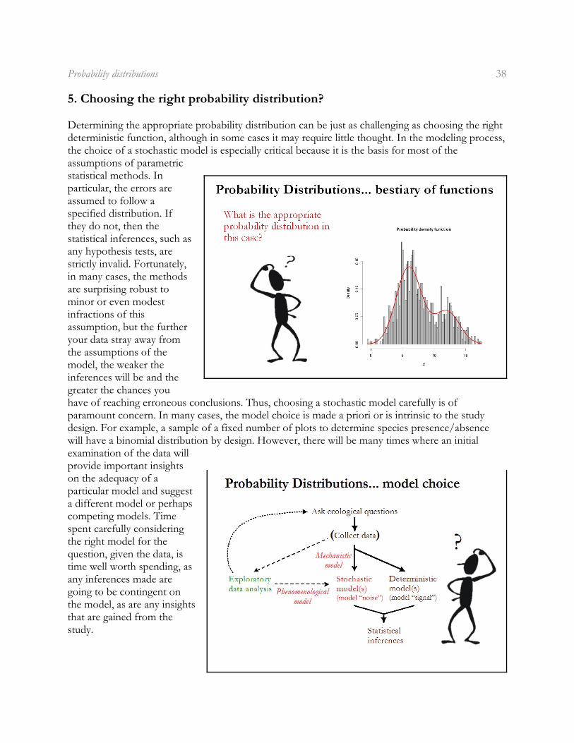
5. Choosing the right probability distribution?

Determining the appropriate probability distribution can be just as challenging as choosing the rightdeterministic function, although in some cases it may require little thought. In the modeling process,the choice of a stochastic model is especially critical because it is the basis for most of theassumptions of parametricstatistical methods. Inparticular, the errors areassumed to follow aspecified distribution. Ifthey do not, then thestatistical inferences, such asany hypothesis tests, arestrictly invalid. Fortunately,in many cases, the methodsare surprising robust tominor or even modestinfractions of thisassumption, but the furtheryour data stray away fromthe assumptions of themodel, the weaker theinferences will be and thegreater the chances youhave of reaching erroneous conclusions. Thus, choosing a stochastic model carefully is ofparamount concern. In many cases, the model choice is made a priori or is intrinsic to the studydesign. For example, a sample of a fixed number of plots to determine species presence/absencewill have a binomial distribution by design. However, there will be many times where an initialexamination of the data willprovide important insightson the adequacy of aparticular model and suggesta different model or perhapscompeting models. Timespent carefully consideringthe right model for thequestion, given the data, istime well worth spending, asany inferences made aregoing to be contingent onthe model, as are any insightsthat are gained from thestudy.


6. Statistical Models – putting it all together

Let’s go back to our three initial real-world examples introduced in the previous section ondeterministic functions and now consider the full statistical model, comprised of both thedeterministic component and the stochastic component, for each example.

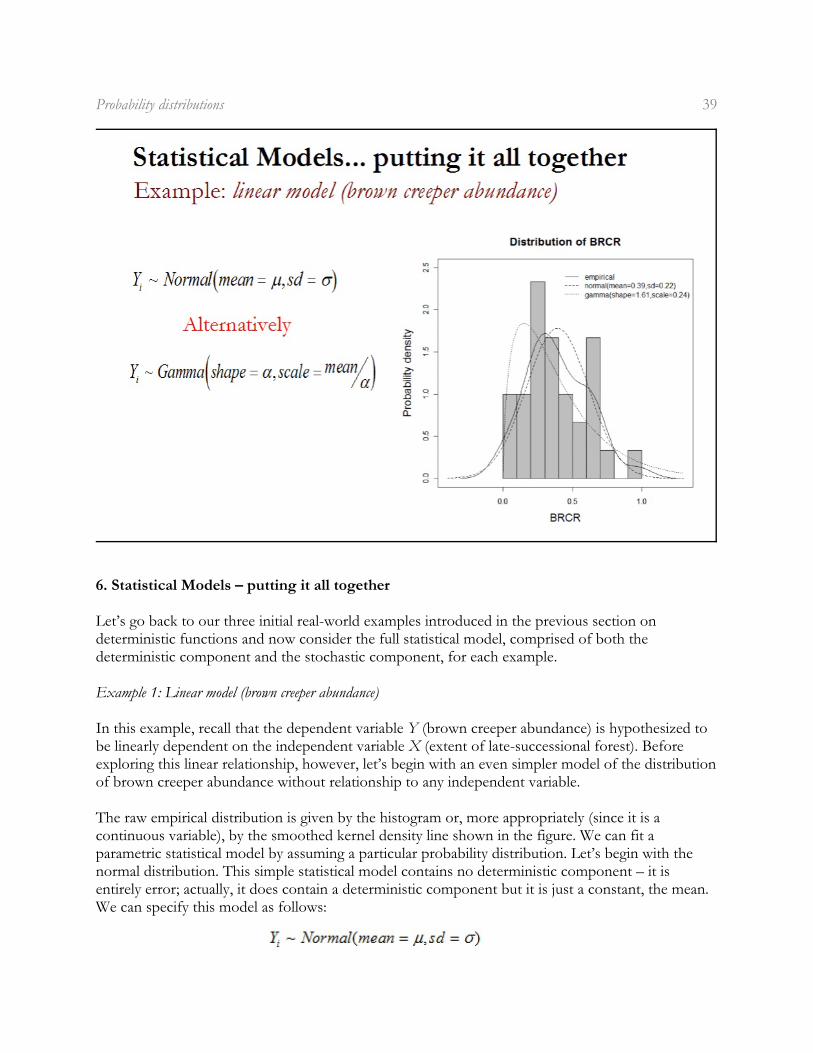
Example 1: Linear model (brown creeper abundance)

In this example, recall that the dependent variable Y (brown creeper abundance) is hypothesized tobe linearly dependent on the independent variable X (extent of late-successional forest). Beforeexploring this linear relationship, however, let’s begin with an even simpler model of the distributionof brown creeper abundance without relationship to any independent variable.

The raw empirical distribution is given by the histogram or, more appropriately (since it is acontinuous variable), by the smoothed kernel density line shown in the figure. We can fit aparametric statistical model by assuming a particular probability distribution. Let’s begin with thenormal distribution. This simple statistical model contains no deterministic component – it isentirely error; actually, it does contain a deterministic component but it is just a constant, the mean.We can specify this model as follows:


Read this as “Y is a random variable distributed (represented by tilda) normally with a mean equal tomu and a standard deviation sd equal to sigma.” If we estimate the mean from the sample mean (0.39)and the standard deviation from sample standard deviation (0.22), the normal distribution matchesthe empirical distribution pretty well as shown in the figure, so the normal probability distributionmight be a reasonable choice for this dataset. However, since the normal distribution allows fornegative values and our random variable (brown creeper abundance) cannot be negative, we mightalso try the Gamma distribution which allows only positive values. We can specify the gamma modelas follows:

Note, in this model there are two parameters, shape and scale. Unfortunately, neither of theseparameters are equal to the mean. The mean of the Gamma is equal to the product of shape andscale. Consequently, we can reparameterize the Gamma as shown, with scale equal to the meandivided by shape. If we were to estimate shape equal to 1.61 and scale equal to 0.24 (mean of Ydivided by 1.61), the Gamma distribution is positively skewed and does not appear to match theempirical distribution as well as the normal.

If we were only interested in describing the distribution of brown creeper abundance, we would bedone with our statistical modeling. However, we are usually interested in trying to explain variationin the dependent variable by one or more independent variables. This is where the deterministicmodel comes into play. We use a deterministic function to model how the expected value of thedependent variable (the mean) varies as some function of the variation in one or more independentvariables. In this example, we want to know if the expected value of brown creeper abundanceincreases linearly with increasing extent of late-successional forest.


In this example, we might hypothesize that the dependent variable Y, brown creeper abundance, islinearly dependent on the independent variable X, extent of late-successional forest, with normallydistributed (and independent) errors. The conventional specification of this model is as follows:

An appealing feature of this model specification is that it makes explicit the distinction between thedeterministic and stochastic components of the model. An alternative and more succinctspecification of this model is as follows:

An appealing feature of this model specification is that it makes explicit the link between thedeterministic and stochastic components of the model. This formulation is the one we will usethroughout and is interpreted as follows: Y is distributed (represented by tilda) normally with a meanequal to a linear function of X and a standard deviation equal to sigma. In this model, there are threeparameters (to be estimated): a and b are the intercept and slope of the linear model and are thusassociated with the deterministic component of the model, and sigma is the standard deviation of thenormal probability distribution and is thus associated with the stochastic component of the model.


Alternatively, we might specify the model with a Gamma error distribution as follows:It is important to recognize the link between the deterministic model and the stochastic model. Inmost cases (including all that we have discussed thus far), the deterministic model is used torepresent how the independent variable(s) relates to the expected value (mean) of the dependent

variable. Thus, the link is via the mean of the probability distribution. Recall that the normalprobability distribution has two parameters: the mean and the standard deviation. If all we areinterested in is explaining the distribution of the dependent variable without relation to anyindependent variable, then we would not have a deterministic model (but in truth, it would simplybe a constant, the meam) and the entire model would be comprised of the stochastic componentalone. In this case, we would have two parameters, the mean and standard deviation. However, if weare interested is explaining the dependent variable in relation to one or more independent variables,which we usually are, then we also need a deterministic model. Instead of simply modeling the meanas a single parameter, we replace the mean parameter with our deterministic function (the linearmodel in this case), which we use in order to specify the mean as a function of an independentvariable. Because the normal distribution has a parameter that is equal to the mean, the link betweenthe deterministic function and the stochastic distribution is straightforward. Unfortunately, this isnot always the case. In the Gamma model, the mean is the product of shape and scale, so we have towork the mean in a little differently. In the case shown here, we specified the scale parameter to beequal to the mean divided by shape. For all practical purposes, this parameterization is no realconcern. We are still modeling the mean as a linear function of the independent variable and theerrors are distributed Gamma about that mean.


Let’s take a graphical look at how the deterministic and stochastic components of the model linktogether. The deterministic linear model (once the slope and intercept parameters have beenestimated) tells us the expected value (mean) of brown creeper abundance. For example, if extent oflate-successional forest is approximately 20%, then we expect or predict brown creeper abundanceto be 0.2. If our data is being generated from a normal distribution, then we expect the observedvalues of brown creeper abundance to vary normally about a mean of 0.2 with a standard deviation(spread) estimated from the data to be 0.14. Thus, for any observed value of brown creeperabundance in a landscape with roughly 20% late-successional forest, we can use the probabilitydensity function to determine the probability of observing that value. Values close to the mean willhave a relatively high probability and values far from the mean will have a relatively low probability.Similarly, if our data is being generated from a Gamma distribution, then we expect the probabilitydensity function to be different. In this case, we estimated the shape to be equal to 3.47 and thus thescale to be equal to 0.2/3.47. The resulting probability distribution gives the probability of observingany particular value of brown creeper abundance if the data came from a Gamma distribution. Note,the Gamma distribution is considerably flatter (i.e., more spread) than the normal and is positivelyskewed, which might be quite reasonable for this data. We can repeat this process for any value ofthe independent variable. For example, if extent of late-successional forest is roughly 80%, then weexpect brown creeper abundance to be 0.6, and the probability of observing any particular value tobe given by the corresponding probability distributions.


Although the probability distribution is determined by the type (and scale) of the dependentvariable, and that should be the paramount consideration in choosing a probability distribution, theformal statistical assumption of the final model is that the residuals (or errors) are (typically)independently and identically distributed according to the specified probability distribution. Thus,the customary way to evaluate the adequacy of a statistical model and whether the statisticalassumptions have been met is to analyze the residuals of the model. One way to do this is simply toplot the residuals and verify that the shape of the distribution is consistent with the chosenprobability distribution.

In the figures shown here, the left plot shows the distribution of the residuals from the model fitwith the Normal errors, and I have overlaid a normal curve with a mean of zero (the expected valuefor the residuals in this case) and a standard deviation estimated from the model fitting process (tobe discussed later). In this case it seems that the residuals plausibly come from a Normaldistribution, although the residual distribution seems to be slightly right-skewed when a Normaldistribution should be perfectly symmetrical. The right plot shows the distribution of the residualsfrom the model fit with Gamma errors, and I have overlaid a Gamma curve (fit by the model) aftershifting the residuals to have a minimum value of zero. In this case, since the Gamma can take onright skew, the distribution seems to correspond better to the observed residuals and we might thusconclude that the Gamma is the more appropriate distribution to use in this case.


Example 2: logistic model (brown creeper presence/absence)

In this example, recall that the dependent variable Y (brown creeper presence) is hypothesized to belogistically dependent on the independent variable X (total basal area). Before exploring thisrelationship, however, let’s begin with a simpler model of the distribution of brown creeper presencewithout relationship to any independent variable.

The raw empirical distribution is given by the barplot shown here. We can fit a parametric statisticalmodel by assuming a particular probability distribution. Let’s assume the binomial distribution,which is perfectly suited for binary response data. This simple statistical model contains nodeterministic component – it is entirely error (but in truth, it is simply a constant, the mean). We can

specify this model as follows:

Read this as “Y is a random variable distributed binomially with a trail size equal to 1 and a per trialprobability of success prob equal to pi.” Note, in this case the trial size if fixed by study design, onlyprob is free to vary. If we estimate the probability of presence to be equal to the proportion ofpresences in our data set (0.32), the binomial distribution matches the empirical distribution exactly– not surprisingly.


Now let’s expand this model to include the logistic relationship between probability of presence andtotal basal area. In this example, the dependent variable Y (probability of brown creeper presence) ishypothesized to vary as a logistic function of the independent variable X (total basal area) withbinomially distributed (and independent) errors. The fully specified model is as follows:

This model is interpreted as follows: ð is the per trial probability of success (presence, in this case)and it is a logistic function of X; Y is distributed binomially with a trial size equal to one and a pertrial probability of success equal to ð. In this model, there are only two parameters (to be estimated):a and b are the location and scale parameters of the logistic function and move the inflection pointleft/right (location) and make the sigmoid curve steeper or shallower (scale). Both parameters areassociated with the deterministic component of the model. There are no additional parameters forthe stochastic component of the model, because the binomial distribution has only one freeparameter when the trial size is fixed at one, and it is the per trial probability of success which isbeing specified via the deterministic model.


As in the previous example, we use the independent variable to predict the mean of the dependentvariable, in this case to determine the expected probability of presence. For example, if total basalarea is roughly 10, then we predict there to be a 0.2 probability of presence. The probability ofobserving either outcome, presence or absence, is then given by the binomial probability massfunction for a trial size equal to 1 and a per trial probability of success equal to 0.2. Similarly, for atotal basal area equal to roughly 60, we predict there to be a 0.8 probability of presence, and thebinomial gives the probability of presence versus absence.


Example 3: Ricker model (striped bass stock-recruitment)

In this example, recall that the dependent variable Y (recruits) is hypothesized presumed to vary as aRicker function of the independent variable X (stock) with either normal or Gamma distributed(and independent) errors. Before exploring this nonlinear relationship, however, let’s begin with aneven simpler model of the distribution of recruits without relationship to any independent variable.

The raw empirical distribution is given by the histogram or, more appropriately (since it is acontinuous variable), by the smoothed kernel density line shown in the figure. We can fit aparametric statistical model by assuming a particular probability distribution. Let’s begin with thenormal distribution. This simple statistical model contains no deterministic component – it isentirely error (but in truth, it is simply a constant, the mean). We can specify this model as follows:

Read this as “Y is a random variable distributed normally with a mean equal to mu and a standarddeviation sd equal to sigma.” If we estimate the mean from the sample mean (9758) and the standarddeviation from sample standard deviation (5213), the normal distribution matches the empiricaldistribution reasonably well as shown in the figure, so the normal probability distribution might be areasonable choice for this dataset. However, since the normal distribution allows for negative valuesand our random variable (recruits) cannot be negative, and the normal distribution is symmetrical


but our data appear to be positively skewed, we might also try the Gamma distribution which allowsonly positive values and allows for positive skew. We can specify the gamma model as follows:Note, as in the first example, we have parameterize the Gamma as shown, with scale equal to themean divided by shape. If we were to estimate shape equal to 1.31 and scale equal to 10000, theGamma distribution is positively skewed and also appears to match the empirical distributionreasonably well.

If we were only interested in describing the distribution of recruits, we would be done with ourstatistical modeling. However, in this example, we want to know if the expected value of recruitsvaries according to a Ricker function of stock.


The fully specified model is as follows:

Alternatively, we can specify the model more succinctly as follows:

This model is interpreted as follows: Y (recruits) is a random variable distributed normally with amean equal to a Ricker function of X (stock) and standard deviation equal to sigma.

Alternatively, we might specify the model with a Gamma error distribution as follows:

In this case, the model is read as follows: Y (recruits) is a random variable distributed Gamma with ashape equal to alpha and scale equal to a Ricker function of X (stock) divided by alpha. In this


model, there are three parameters (to be estimated): a and b are parameters of the Ricker functionand influence the location and shape of the curve and are thus associated with the deterministiccomponent of the model, and alpha is the shape parameter of the Gamma distribution and is thusassociated with the stochastic component of the model. Note, the mean of the Gamma distributionis equal to the product of the scale parameter and the shape parameter (see Bolker). Thus, to link thedeterministic model to the stochastic model, we have to redefine the scale parameter to be equal tothe mean (expected value of Y) divided by shape.


Now let’s take a graphical look at how the deterministic and stochastic components of the modellink together. Once the parameters of the deterministic model (a and b) have been estimated, it tellsus the expected value (mean) of the dependent variable recruits. For example, if stock isapproximately 1000, then we expect or predict recruits to be roughly 7500. If our data is beinggenerated from a normal distribution, then we expect the observed values of recruits to varynormally about a mean of 7500 with a standard deviation (spread) estimated from the data to be1099. Thus, for any observed value of recruits coming from a stock of roughly 1000, we can use theprobability density function to determine the probability of observing that value. Values close to themean will have a relatively high probability and values far from the mean will have a relatively lowprobability. Similarly, if our data is being generated from a Gamma distribution, then we expect theprobability density function to be different. In this case, we estimated the shape to be equal to 12.91and thus the scale to be equal to 7500/12.91. The resulting probability distribution gives theprobability of observing any particular value of recruits if the data came from a Gamma distribution.Note, the Gamma distribution is considerably flatter (i.e., more spread) than the normal and ispositively skewed, which might be quite reasonable for this data. We can repeat this process for anyvalue of the independent variable. For example, if stock is roughly 5000, then we expect recruits tobe 1350, and the probability of observing any particular value to be given by the correspondingprobability distributions.


In the figures shown here, the left plot shows the distribution of the residuals from the model fitwith the Normal errors, and I have overlaid a normal curve with a mean of zero (the expected valuefor the residuals in this case) and a standard deviation estimated from the model fitting process (tobe discussed later). In this case it seems that the residuals plausibly come from a Normaldistribution, although the residual distribution seems to be slightly right-skewed when a Normaldistribution should be perfectly symmetrical. The right plot shows the distribution of the residualsfrom the model fit with Gamma errors, and I have overlaid a Gamma curve (fit by the model) aftershifting the residuals to have a minimum value of zero. In this case, since the Gamma can take onright skew, the distribution seems to correspond better to the observed residuals and we might thusconclude that the Gamma is the more appropriate distribution to use in this case.

Date post:	24-Apr-2018
Category:	Documents
Upload:	trankhanh
View:	220 times
Download:	0 times

Analysis of Environmental Data - UMass Amherst · Probability distributions 7 1.3 Probability...

Documents