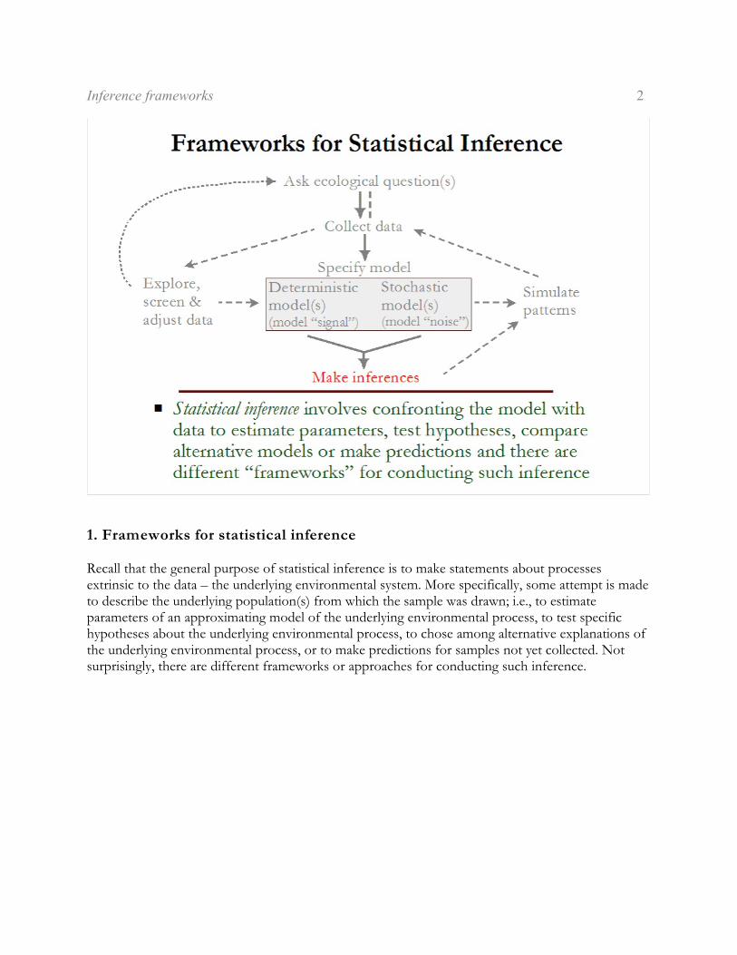
Recall that the general purpose of statistical inference is to make statements about processesextrinsic to the data – the underlying environmental system. More specifically, some attempt is madeto describe the underlying population(s) from which the sample was drawn; i.e., to estimateparameters of an approximating model of the underlying environmental process, to test specifichypotheses about the underlying environmental process, to chose among alternative explanations ofthe underlying environmental process, or to make predictions for samples not yet collected. Notsurprisingly, there are different frameworks or approaches for conducting such inference.
Inference frameworks 3
Parametric inference.–In modern statistics there are two major conceptual frameworks (or paradigms)for conducting parametric statistical inference – classical frequentist and Bayesian. Both of theseframeworks require statistical models to assume a known probability distribution for the stochasticcomponent, which makes them “parametric”. Maximum likelihood is sometimes described as a thirdframework, but it is really just a particular approach within the general frequentist framework. Thedistinction between these frameworks is sometimes blurred, since maximum likelihood and Bayesianmethods are both based on the likelihood – the probability of the observed data given a particularmodel or choice of parameters. Thus, likelihood serves as a bridge between the frequentist andBayesian frameworks.
Nonparametric inference.–Sometimes it is not possible to assume any particular error distribution for themodel and “nonparametric” statistical methods must be used. Inferences derived fromnonparametric methods are generally much weaker than those from parametric methods, becausewithout a probability distribution for the error it is difficult to conceive of the statistical model as adata-generating mechanism for the underlying environmental system. For example, there is no easyway to simulate data from a model without specifying a probability distribution for the error. Moreover, even if we can estimate the parameters of the model, without a probability distribution itis impossible to say whether these are the most likely or probable values for the underlyingpopulation. In fact, nonparametric inference really isn’t a conceptual framework or paradigm forconducting statistical inference at all, it’s more like the lack of an inference framework. Nevertheless,we include it here as a “framework” because there are many occasions when nonparametric methodsare useful or required.
Inference frameworks 4
2. Philosophical distinction between parametric frameworks
The frequentist and Bayesian inference frameworks can be thought of as more than meremethodological frameworks, but as philosophies as well.
Frequentist.–The frequentist generally believes that there is a true underlying model (and parameters)that defines the way the environmental system works, which we cannot perfectly observe?Consequently, the parameters are assumed to be fixed but unknown, while the sample data areviewed as a random outcome of the underlying model; i.e., an imperfect representation of theunderlying truth. The frequentist asks: what is the probability of observing the sample data given thefixed parameters, and finds the values (estimates) of those parameters that would make the data themost likely (frequently occurring) outcome under repeated sampling of the system (if one were ableto repeatedly sample the system).
Bayesian.–The Bayesian, on the other hand, generally believes that the only knowable truth is thesample data itself and therefore does not worry about whether there are true fixed parameters ornot. Consequently, the sample data is assumed to be true (since it is observed), while the modelparameters are viewed as random variables. Accordingly, the Bayesian asks: what is the probability ofthe model (parameters) given the observed data (and prior expectations), and finds the populationparameters that are most probable.
Inference frameworks 5
3. Classical frequentist inference framework
Classical frequentist inference (due to Fisher, Neyman, and Pearson) is simply one of the ways inwhich we can make statistical inferences and is the one that is typically presented in introductorystatistics classes. The essence of the approach is as follows:
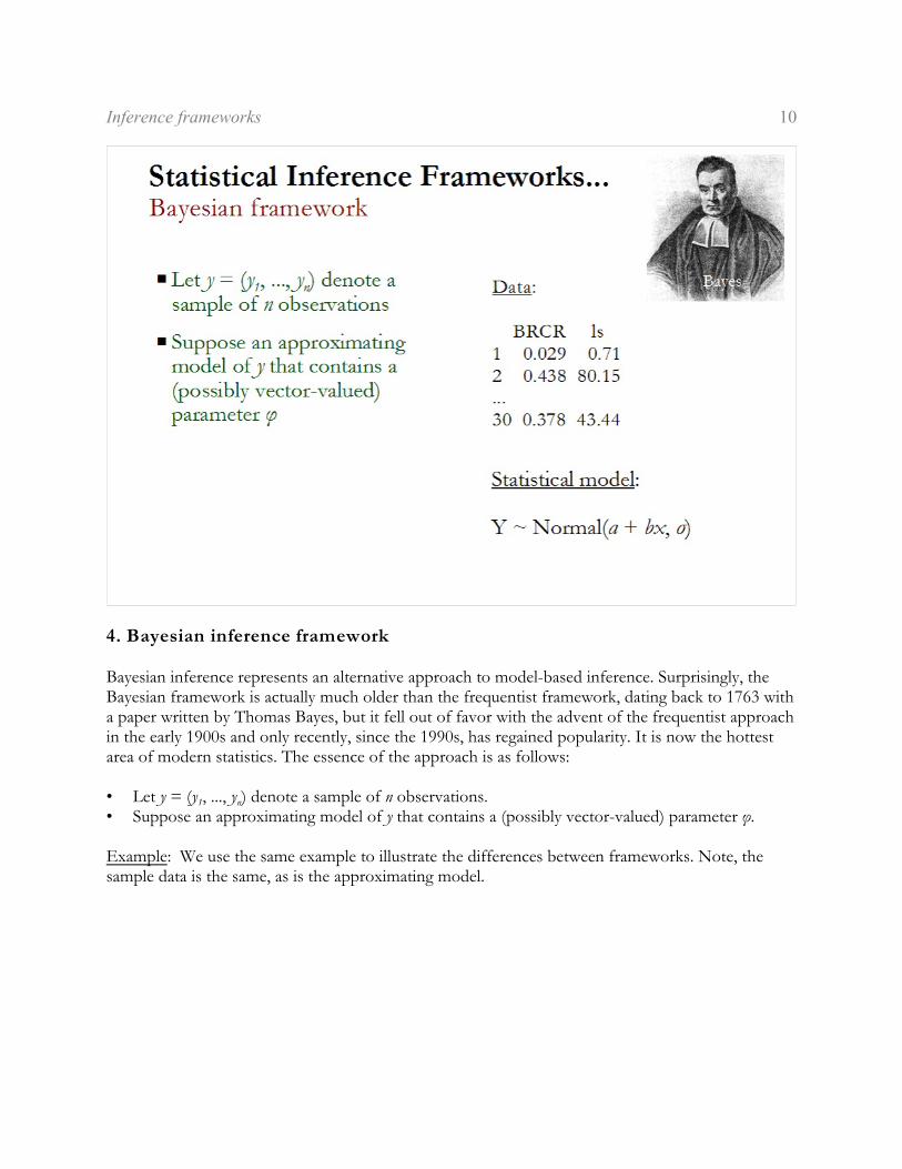
1 n• Let y = (y , ..., y ) denote a sample of n observations.• Suppose an approximating model of y that contains a (possibly vector-valued) parameter ö.
Example: We illustrate the approach using a simple ecological model based on the now familiarOregon birds data set. For this example, let’s examine the relationship between brown creeperabundance and the extent of late-successional forest across 30 subbasins in the central Oregon CoastRange based on the real data collected. For now, we will ignore the real data and simply simulatesome data based on a particular statistical model. Let’s assume a linear model (deterministiccomponent) with normal errors (stochastic component), which we can write as:
Y ~ Normal(a + bx, ó)
which specifies that Y (brown creeper abundance) is a random variable drawn from a normaldistribution with a mean a + bx and standard deviation ó. In this notation, a and b are parameters ofthe deterministic linear model (intercept and slope, respectively), x is data (%late-successionalforest), and ó is a parameter of the stochastic component of the model (the standard deviation of the
i inormally distributed errors). This means that the i value of Y, y , is equal to a + bx plus a normallyth
distributed error with mean equal to the linear model and variance ó .2
Inference frameworks 6
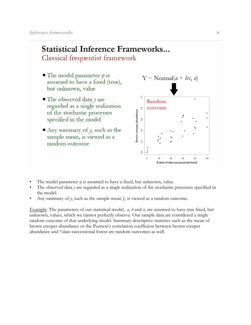
• The model parameter ö is assumed to have a fixed, but unknown, value.• The observed data y are regarded as a single realization of the stochastic processes specified in
the model.• Any summary of y, such as the sample mean Gy , is viewed as a random outcome.
Example: The parameters of our statistical model, a, b and ó, are assumed to have true fixed, butunknown, values, which we cannot perfectly observe. Our sample data are considered a singlerandom outcome of that underlying model. Summary descriptive statistics such as the mean ofbrown creeper abundance or the Pearson’s correlation coefficient between brown creeperabundance and %late-successional forest are random outcomes as well.
Inference frameworks 7
• A procedure for estimating the value of ö is called an estimator and the result of its application toa particular data set yields an estimate of the fixed parameter ö.
• The estimate is viewed as a random outcome because it is a function of y, which is also regardedas a random outcome.
Example: Here we used the method of ordinary least squares (OLS) to estimate the values of theparameters a, b and ó, but we could have just as easily used the method of maximum likelihoodestimation (MLE). Under the assumptions of this model, namely that the errors are normallydistribution, these two methods produce equivalent point estimates of the parameters. For now, weneed not worry about the details of the particular estimation method (more on this in the nextchapters). Suffice it to say that either method produces parameter estimates that make our observeddata the most likely outcome under repeated sampling.
Inference frameworks 8
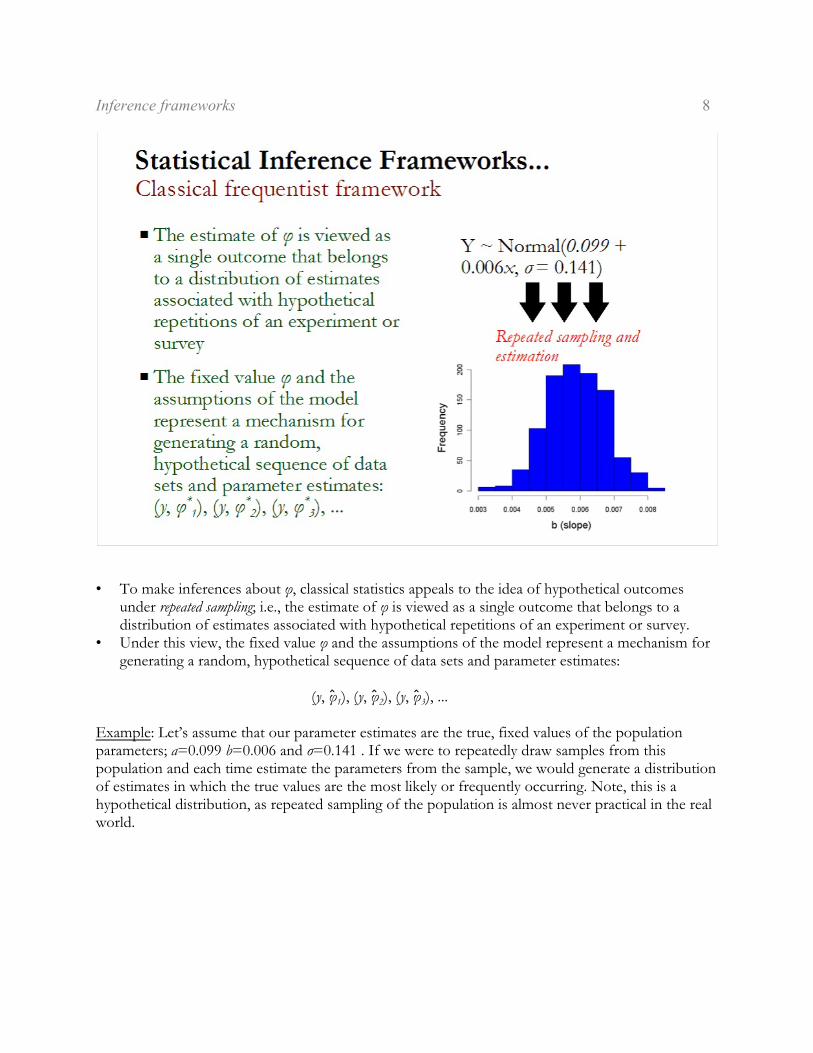
• To make inferences about ö, classical statistics appeals to the idea of hypothetical outcomesunder repeated sampling; i.e., the estimate of ö is viewed as a single outcome that belongs to adistribution of estimates associated with hypothetical repetitions of an experiment or survey.
• Under this view, the fixed value ö and the assumptions of the model represent a mechanism forgenerating a random, hypothetical sequence of data sets and parameter estimates:
1 2 3(y, ö8 ), (y, ö8 ), (y, ö8 ), ...
Example: Let’s assume that our parameter estimates are the true, fixed values of the populationparameters; a=0.099 b=0.006 and ó=0.141 . If we were to repeatedly draw samples from thispopulation and each time estimate the parameters from the sample, we would generate a distributionof estimates in which the true values are the most likely or frequently occurring. Note, this is ahypothetical distribution, as repeated sampling of the population is almost never practical in the realworld.
Inference frameworks 9
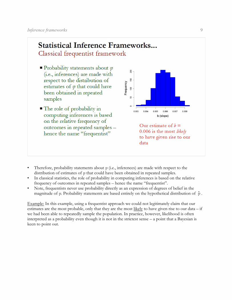
• Therefore, probability statements about ö (i.e., inferences) are made with respect to thedistribution of estimates of ö that could have been obtained in repeated samples.
• In classical statistics, the role of probability in computing inferences is based on the relativefrequency of outcomes in repeated samples – hence the name “frequentist”.
• Note, frequentists never use probability directly as an expression of degrees of belief in themagnitude of ö. Probability statements are based entirely on the hypothetical distribution of ö8 .
Example: In this example, using a frequentist approach we could not legitimately claim that ourestimates are the most probable, only that they are the most likely to have given rise to our data – ifwe had been able to repeatedly sample the population. In practice, however, likelihood is ofteninterpreted as a probability even though it is not in the strictest sense – a point that a Bayesian iskeen to point out.
Inference frameworks 10
4. Bayesian inference framework
Bayesian inference represents an alternative approach to model-based inference. Surprisingly, theBayesian framework is actually much older than the frequentist framework, dating back to 1763 witha paper written by Thomas Bayes, but it fell out of favor with the advent of the frequentist approachin the early 1900s and only recently, since the 1990s, has regained popularity. It is now the hottestarea of modern statistics. The essence of the approach is as follows:
1 n• Let y = (y , ..., y ) denote a sample of n observations.• Suppose an approximating model of y that contains a (possibly vector-valued) parameter ö.
Example: We use the same example to illustrate the differences between frameworks. Note, thesample data is the same, as is the approximating model.
Inference frameworks 11
• In frequentist inference, the model parameter ö is assumed to have a fixed, but unknown, value.In Bayesian inference, the model parameter è is treated as a random variable and theapproximating model is elaborated to include a probability distribution for ö that specifies one’sbeliefs about the magnitude of ö prior to having observed the data – this elaboration is called theprior distribution. The prior distribution is necessary in order to make the Bayesian approach work,but we will not worry about that here.
Example: The parameters of our statistical model, a, b and ó, are treated as random variables, notfixed as in the frequentist approach. In fact, in the Bayesian approach, it is mute whether theparameters are believed to be truly fixed or not since we can never confirm them as such. The bestwe can do is make probability statements about their values. Importantly, in the Bayesian approachwe have to specify our prior belief about the values of the parameters. For example, we mightspecify our prior belief that the slope parameter (b) in the linear model is normally distributed with amean of 0.004 and a standard deviation of 0.001 and then see whether the sample data conforms tothis expectation or differs.
Inference frameworks 12
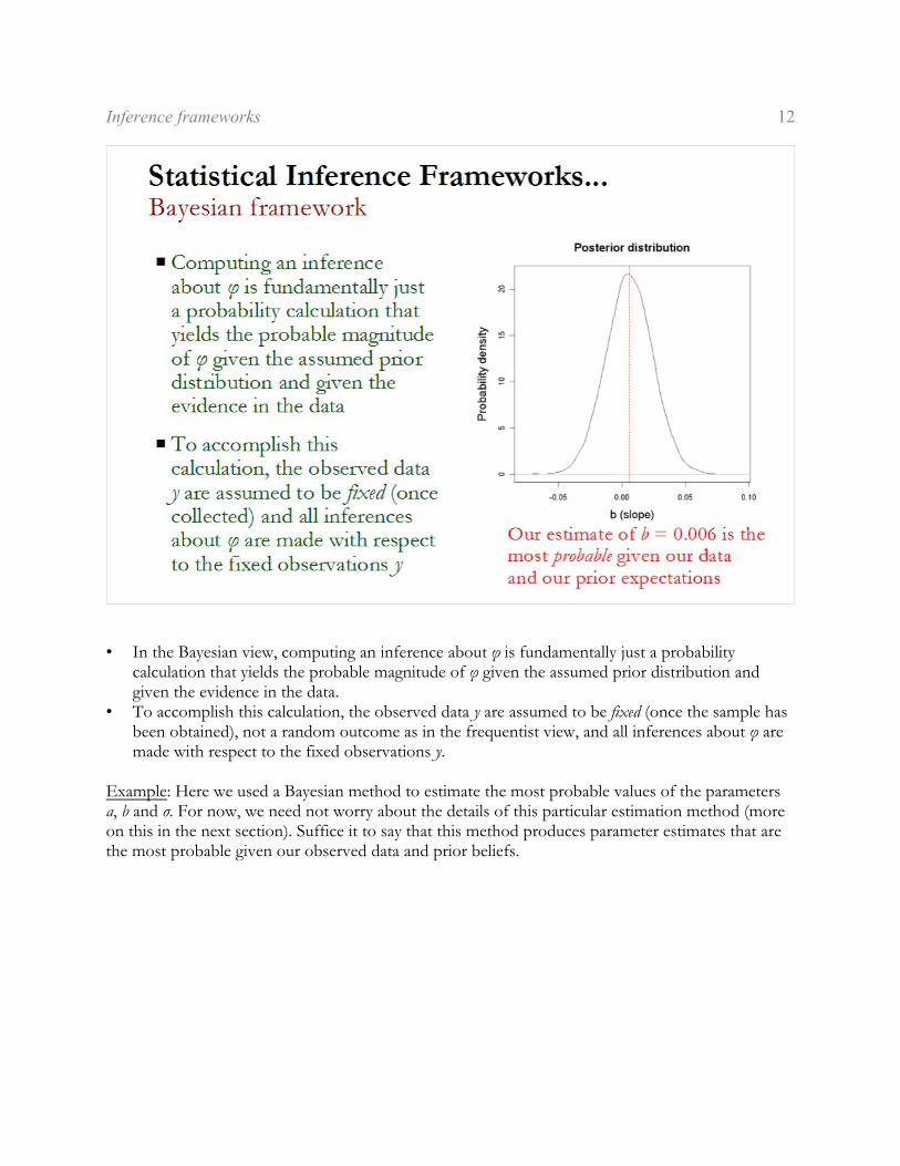
• In the Bayesian view, computing an inference about ö is fundamentally just a probabilitycalculation that yields the probable magnitude of ö given the assumed prior distribution andgiven the evidence in the data.
• To accomplish this calculation, the observed data y are assumed to be fixed (once the sample hasbeen obtained), not a random outcome as in the frequentist view, and all inferences about ö aremade with respect to the fixed observations y.
Example: Here we used a Bayesian method to estimate the most probable values of the parametersa, b and ó. For now, we need not worry about the details of this particular estimation method (moreon this in the next section). Suffice it to say that this method produces parameter estimates that arethe most probable given our observed data and prior beliefs.
Inference frameworks 13
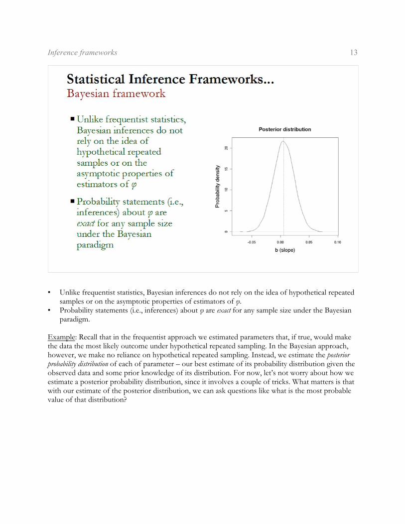
• Unlike frequentist statistics, Bayesian inferences do not rely on the idea of hypothetical repeatedsamples or on the asymptotic properties of estimators of ö.
• Probability statements (i.e., inferences) about ö are exact for any sample size under the Bayesianparadigm.
Example: Recall that in the frequentist approach we estimated parameters that, if true, would makethe data the most likely outcome under hypothetical repeated sampling. In the Bayesian approach,however, we make no reliance on hypothetical repeated sampling. Instead, we estimate the posteriorprobability distribution of each of parameter – our best estimate of its probability distribution given theobserved data and some prior knowledge of its distribution. For now, let’s not worry about how weestimate a posterior probability distribution, since it involves a couple of tricks. What matters is thatwith our estimate of the posterior distribution, we can ask questions like what is the most probablevalue of that distribution?
Inference frameworks 14
5. Comparison of Inference frameworks
The classical frequentist and Bayesian inference frameworks differ in a number of important andsome not so important ways. Each framework has proponents that are quick to point out thedrawbacks of the other. Let’s review a few of the more notable differences and opposing points ofview here; we will address additional points of comparison later.
1. Random model versus random data.–Implicit in the frequentist approach to estimation is that there is afixed quantity in nature, the parameter(s), that we wish to measure. In short, for a frequentist it isparameters that are fixed while it is the data that are random. This is diametrically opposed to theBayesian point of view. For a Bayesian it is the data that are fixed while the parameters are random.Since we can never know whether any model is true, Bayesians argue that it does not make sense tocondition on something we can never observe. Bayesians argue that we should instead determine theprobability of the model given the data (i.e., condition on the data), since the data is the only thingwe know for certain.
The notion that the parameter is a fixed quantity in nature causes problems in interpretation for thefrequentist. When estimating a parameter we usually derive both point and interval estimates. Thepoint estimate is our best guess at the parameter’s true value; the interval estimate is our best guessat the likely interval (range of values) that contains the parameter’s true value. When we constructthe interval estimate (called a confidence interval) for a parameter, we like to treat the interval as a
Inference frameworks 15
probability statement for the parameter—a set of likely values. But in truth, if the parameter is fixed,then it is either in the interval we've constructed or it's not. There's no probability associated with it.The probability instead derives from the sampling distribution. For example, we call it a 95%confidence interval because we're guaranteed that 95% of the intervals we might have constructed ifwe had obtained all possible samples from the population do in fact contain the true parametervalue. All we can do is hope that this is one of the lucky ones. The bottom line is that when theparameter is treated as real and fixed, then it's only our methods that can have probability associatedwith them.
As far as the existence of a true value of the parameter in nature, Bayesians are of an open mind.The parameter may or may not be real, but in the Bayesian perspective it doesn't matter. All weknow about the parameter is what we believe about it. As knowledge accumulates, our beliefs aboutthe parameter become more focused. Since the value of the parameter is a matter of belief, andprobability is a matter of belief, for all intents and purposes the parameter can be viewed as arandom quantity. Consequently, to a Bayesian, parameters are random variables, not fixed constants.As a result, confidence intervals pose no philosophical dilemma for a Bayesian. Since parameters arerandom, we can make probability statements about their values. Thus, a confidence interval for aparameter is a probability statement about the likely values of the parameter. To avoid confusionwith frequentist confidence intervals, Bayesians often call their intervals "credibility intervals".
Inference frameworks 16
2. Reliance on hypothetical repeated sampling.–For the frequentist, everything hinges on the notion ofrepeated sampling to generate the sampling distribution of the statistic. Here, the definition ofprobability depends on a series of hypothetical repeated experiments that are often impossible in anypractical sense. Importantly, in the frequentist framework, we assume that the specified model is trueand that the data represent a random outcome. We try to estimate the parameters of the model thatif true would give rise to our observed data as the most frequently occurring outcome. For example,to say that the probability of heads is one half when a fair coin is tossed once means that if we wereto flip a fair coin repeatedly the long run relative frequency of heads is one half. But since we onlyobserve our data once (typically), we have to estimate the parameters that would have given rise toour data more frequently than any other set of observations if we had been able to repeatedlyresample the population. Because we can almost never actually do this in the real world, Bayesiansfind this framework silly.
For the Bayesian, there is no reliance on hypothetical repeated sampling. The probabilisticinterpretation of parameters instead stems from the fact that parameters are treated as randomvariables, not fixed constants, which allows us to make probability statements about their valuesdirectly. However, the catch is that to do this we have to specify prior probability distributions foreach parameter – our prior belief in the value of each parameter. Given the data in hand and theseprior distributions, we can derive parameter estimates that are the most probable values – withouthypothetical repeated sampling. Frequentists object to the use of priors.
Inference frameworks 17
3. Role of priors - subjective versus objective approaches.--A Bayesian takes pride in the fact that the Bayesianmethod of estimation, which finds the most probable parameters given the data at hand and priorknowledge, essentially encapsulates inductive science in a single formula. In science we developtheories about nature. Observation and experiment then cause us to modify those theories aboutnature. Further data collection causes further modification. Thus, science is a constant dynamicbetween prior and posterior probabilities, with prior probabilities becoming modified into posteriorprobabilities through experimentation at which point they become the prior probabilities of futureexperiments. Thus, the Bayesian perspective accounts for the cumulative nature of science.
The frequentist retort is that this is a mischaracterization of science. Science is inherently objectiveand has no use for subjective quantities such as prior probabilities. Science should be based on dataalone and not the prejudices of the researcher.
The Bayesian rejoinder is first that science does have a subjective component. The "opinions" ofscientists dictate the kinds of research questions they pursue. In any case, if there is concern that aprior probability unfairly skews the results, the analysis can be rerun with other priors or withuninformative priors that do not skew the results in any direction. In fact, in Bayesian analysis it isfairly typical to carry out analyses with a range of priors to demonstrate that results are robust to thechoice of prior. In any event, with large sample sizes, say >30, the priors may have little influence onthe result anyways.
In fact both schools of thought are correct here. While Bayesians may have described the idealscientific method, in truth consensus in science is informal at best. Perhaps there should be a currentprior probability in vogue for everything in science, but typically there isn't. Without this consensusthe inherent subjectivity of priors does seem to be a problem, at least in some cases.
Inference frameworks 18
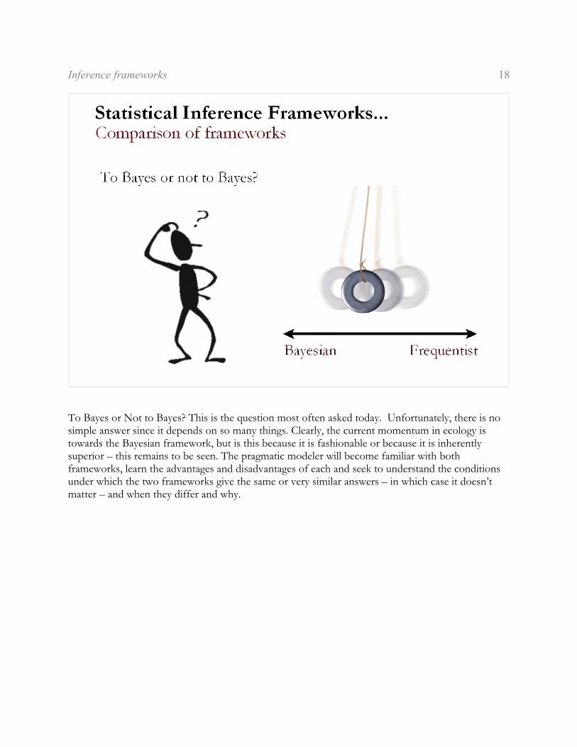
To Bayes or Not to Bayes? This is the question most often asked today. Unfortunately, there is nosimple answer since it depends on so many things. Clearly, the current momentum in ecology istowards the Bayesian framework, but is this because it is fashionable or because it is inherentlysuperior – this remains to be seen. The pragmatic modeler will become familiar with bothframeworks, learn the advantages and disadvantages of each and seek to understand the conditionsunder which the two frameworks give the same or very similar answers – in which case it doesn’tmatter – and when they differ and why.