University of Tennessee, Knoxville University of Tennessee, Knoxville TRACE: Tennessee Research and Creative TRACE: Tennessee Research and Creative Exchange Exchange Masters Theses Graduate School 5-2011 ANALYSIS OF FACTORS AFFECTING FARMERS’ WILLINGNESS TO ANALYSIS OF FACTORS AFFECTING FARMERS’ WILLINGNESS TO ADOPT SWITCHGRASS PRODUCTION IN THE SOUTHERN UNITED ADOPT SWITCHGRASS PRODUCTION IN THE SOUTHERN UNITED STATES AND AN EXCEL SPREADSHEET-BASED DECISION TOOL STATES AND AN EXCEL SPREADSHEET-BASED DECISION TOOL FOR POTIENTIAL SWITCHGRASS PRODUCERS FOR POTIENTIAL SWITCHGRASS PRODUCERS Donald Joshua Qualls [email protected]Follow this and additional works at: https://trace.tennessee.edu/utk_gradthes Recommended Citation Recommended Citation Qualls, Donald Joshua, "ANALYSIS OF FACTORS AFFECTING FARMERS’ WILLINGNESS TO ADOPT SWITCHGRASS PRODUCTION IN THE SOUTHERN UNITED STATES AND AN EXCEL SPREADSHEET-BASED DECISION TOOL FOR POTIENTIAL SWITCHGRASS PRODUCERS. " Master's Thesis, University of Tennessee, 2011. https://trace.tennessee.edu/utk_gradthes/933 This Thesis is brought to you for free and open access by the Graduate School at TRACE: Tennessee Research and Creative Exchange. It has been accepted for inclusion in Masters Theses by an authorized administrator of TRACE: Tennessee Research and Creative Exchange. For more information, please contact [email protected].
Transcript
University of Tennessee, Knoxville University of Tennessee, Knoxville
TRACE: Tennessee Research and Creative TRACE: Tennessee Research and Creative
Exchange Exchange
Masters Theses Graduate School
5-2011
ANALYSIS OF FACTORS AFFECTING FARMERS’ WILLINGNESS TO ANALYSIS OF FACTORS AFFECTING FARMERS’ WILLINGNESS TO
ADOPT SWITCHGRASS PRODUCTION IN THE SOUTHERN UNITED ADOPT SWITCHGRASS PRODUCTION IN THE SOUTHERN UNITED
STATES AND AN EXCEL SPREADSHEET-BASED DECISION TOOL STATES AND AN EXCEL SPREADSHEET-BASED DECISION TOOL
FOR POTIENTIAL SWITCHGRASS PRODUCERS FOR POTIENTIAL SWITCHGRASS PRODUCERS
Follow this and additional works at: https://trace.tennessee.edu/utk_gradthes
Recommended Citation Recommended Citation Qualls, Donald Joshua, "ANALYSIS OF FACTORS AFFECTING FARMERS’ WILLINGNESS TO ADOPT SWITCHGRASS PRODUCTION IN THE SOUTHERN UNITED STATES AND AN EXCEL SPREADSHEET-BASED DECISION TOOL FOR POTIENTIAL SWITCHGRASS PRODUCERS. " Master's Thesis, University of Tennessee, 2011. https://trace.tennessee.edu/utk_gradthes/933
This Thesis is brought to you for free and open access by the Graduate School at TRACE: Tennessee Research and Creative Exchange. It has been accepted for inclusion in Masters Theses by an authorized administrator of TRACE: Tennessee Research and Creative Exchange. For more information, please contact [email protected].
I am submitting herewith a thesis written by Donald Joshua Qualls entitled "ANALYSIS OF
FACTORS AFFECTING FARMERS’ WILLINGNESS TO ADOPT SWITCHGRASS PRODUCTION IN
THE SOUTHERN UNITED STATES AND AN EXCEL SPREADSHEET-BASED DECISION TOOL FOR
POTIENTIAL SWITCHGRASS PRODUCERS." I have examined the final electronic copy of this
thesis for form and content and recommend that it be accepted in partial fulfillment of the
requirements for the degree of Master of Science, with a major in Agricultural Economics.
Kimberly L. Jensen, Major Professor
We have read this thesis and recommend its acceptance:
Burton C. English, Daniel G. de la Torre Ugarte
Accepted for the Council:
Carolyn R. Hodges
Vice Provost and Dean of the Graduate School
(Original signatures are on file with official student records.)
ANALYSIS OF FACTORS AFFECTING FARMERS’ WILLINGNESS TO ADOPT
SWITCHGRASS PRODUCTION IN THE SOUTHERN UNITED STATES
ANDAN EXCEL SPREADSHEET-BASED DECISION TOOL FOR POTIENTIAL
SWITHGRASS
PRODUCERS
A Thesis
Presented for the Master of Science Degree
The University of Tennessee, Knoxville
Donald Joshua Qualls
May 2011
ii
ABSTRACT
The increased need for and scarcity of hydrocarbon energy pushes the search and extraction of
reserves toward more technically difficult deposits and less efficient forms of hydrocarbon energy. The
increased use of hydrocarbons also predicates the increased emission of detrimental chemicals in our
surrounding environment. For these reasons, there is a need to find feasible sources of renewable energy
that could prove to be more environmentally friendly.
One possible source that meets these criteria is biomass, which in the United States is the largest
source of renewable energy as it accounts for over 3 percent of the energy consumed domestically and is
currently the only source for liquid renewable transportation fuels. Continued development of biomass
as a renewable energy source is being driven in large part by the Energy Independence and Security Act
of 2007 that mandates that by 2022 at least 36 billion gallons of fuel ethanol be produced, with at least
16 billion gallons being derived from cellulose, hemi-cellulose, or lignin. However, the production of
biomass has drawbacks. The market for cellulosic bio-fuel feedstock is still under development, and
being an innovative technique, there is a lack of production knowledge on the side of the producer.
Some studies have been conducted that determine farmers’ willingness to produce switchgrass,
however, they have been limited in geographic scope and additional research is warranted considering a
broader area. Also, there have been production decision tools aimed at bio-mass, but these have either
not been aimed at switchgrass specifically or have been missing key costs such as those incurred in
storage. The overall objectives of this study are: 1.) to analyze the willingness of producers in the
southeastern United States to plant switchgrass as a biofuel feedstock, 2.) to estimate the area of
switchgrass they would be willing to plant at different switchgrass prices, 3.) to evaluate the factors that
influence a producer’s decision to convert acreage to switchgrass, and 4.) to present a spreadsheet-based
decision tool for potential switchgrass producers.
iii
Table of Contents Part 1: Introduction ......................................................................................................................................1
Part 2: Analysis of Factors Affecting Farmers’ Willingness to Adopt Switchgrass Production in the Southeastern United States ..............................................................................................................9
Review of Literature ..................................................................................................................................14
Data ................................................................................................................................................33
Part 3: An Excel Spreadsheet-Based Decision Tool for Potential Switchgrass Producers . 65 Introduction....................................................................................................................................................................66
Literature Review.......................................................................................................................................69
Case Study .................................................................................................................................................71 Methods......................................................................................................................................................71
References ..................................................................................................................................................98 Part 4: Conclusions ..................................................................................................................................101 Conclusions ..............................................................................................................................................102 Vita ...........................................................................................................................................................105
v
LIST OF TABLES Table A.1. Farm and farmer demographics for the sample .................................................................47
Table A.2. Farm and farmer demographics for the sample cont. .......................................................48
Table A.3. Familiarity and interest in growing switchgrass as an energy crop ...................................49
Table A.8. Variable means and estimated values ................................................................................54
Table A.9. Estimated Tobit model with sample selection ...................................................................55
vi
LIST OF FIGURES Figure 1. The input section of the input-output sheet ........................................................................73
Figure 2. The output section of the input-output sheet .....................................................................74
Figure 3. The per acre section of the cash flow sheet. .....................................................................76
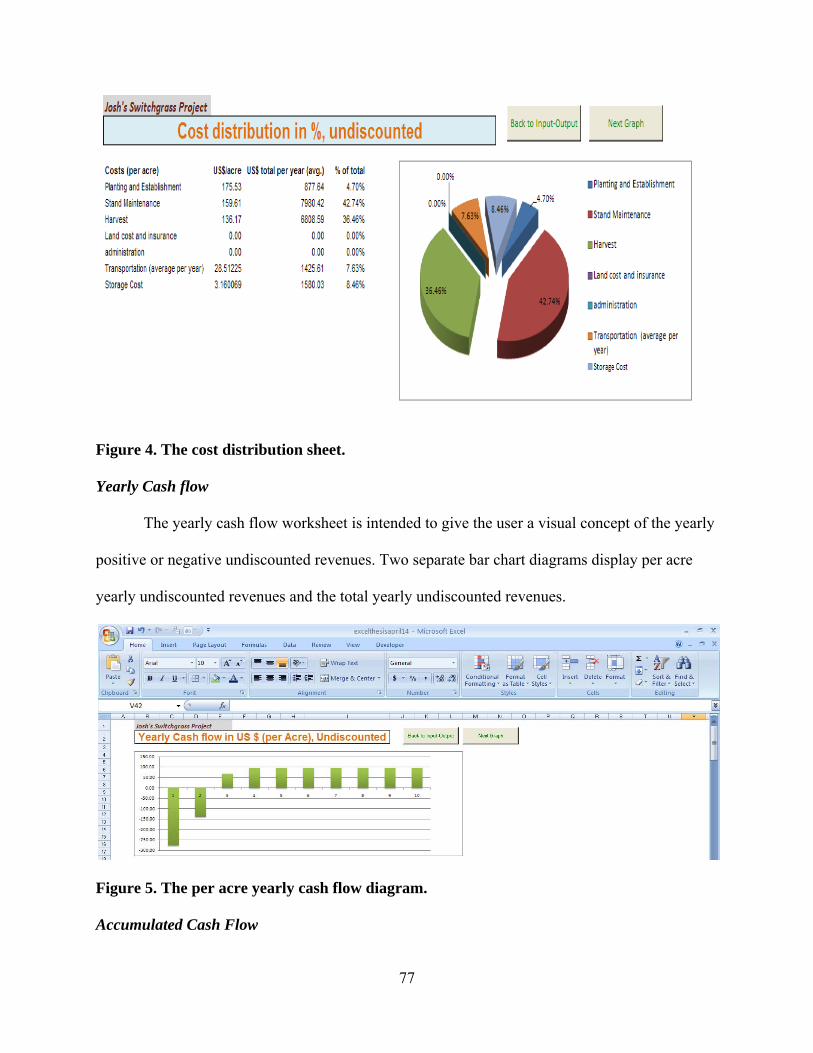
Figure 4. The cost distribution sheet. ...............................................................................................77
Figure 5. The per acre yearly cash flow diagram. ............................................................................77
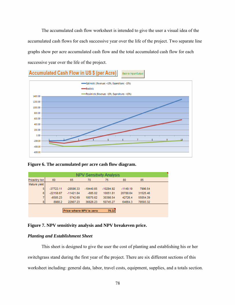
Figure 6. The accumulated per acre cash flow diagram. ..................................................................78
Figure 7. NPV sensitivity Analysis and NPV Breakdown Price .......................................................78
Figure 8. The general data, labor, and travel costs subsections of the planting and establishment sheet. ..................................................................................................................................80
Figure 9. the equipment costs subsection of the planting and establishment sheet ..........................82
Figure 10. The supplies costs and the total cost subsections of the planting and establishment sheet.............................................................................................................................................83
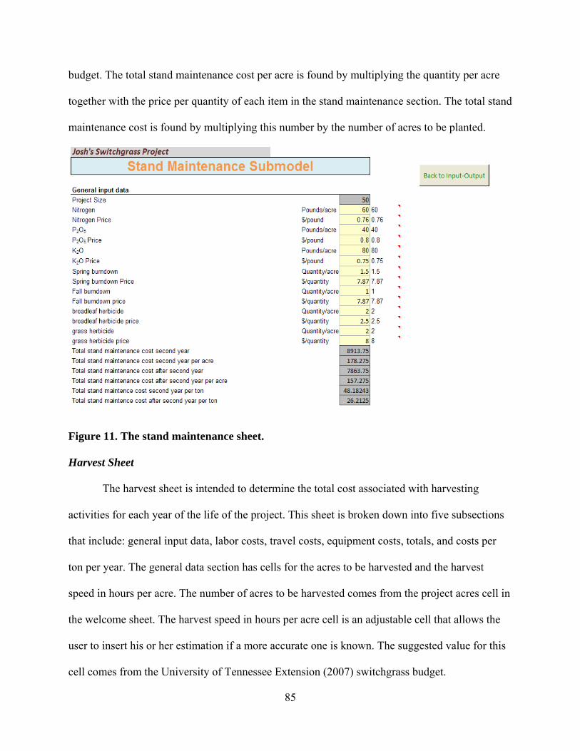
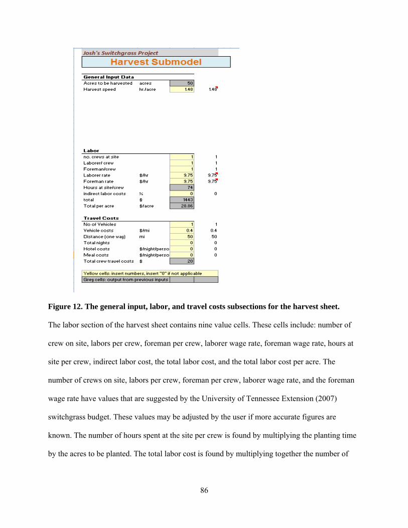
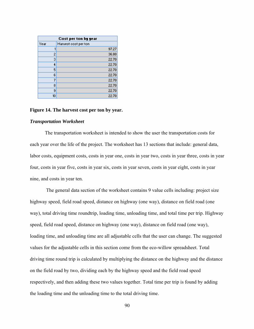
Figure 11. The stand maintenance sheet. ............................................................................................85 Figure 12. The general input, labor, and travel costs subsections for the harvest sheet .....................86 Figure 13. The equipment costs subsections of the harvest sheet .......................................................89 Figure 14. The harvest costs per ton by year .......................................................................................90 Figure 15. The general data, labor costs, and equipment costs subsections of the transportation sheet.
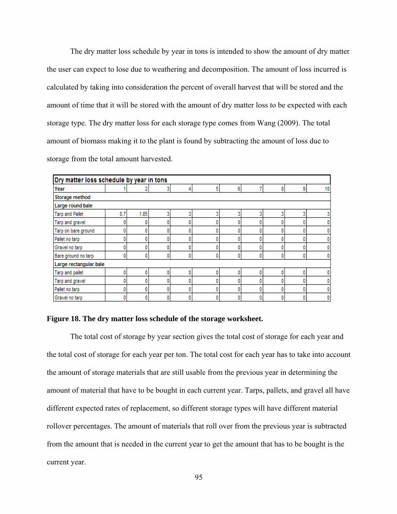
............................................................................................................................................92 Figure 16. The yearly transportation costs of the transportation worksheet. ......................................93 Figure 17. The general data, bailing method, storage time, and storage method subsections of the
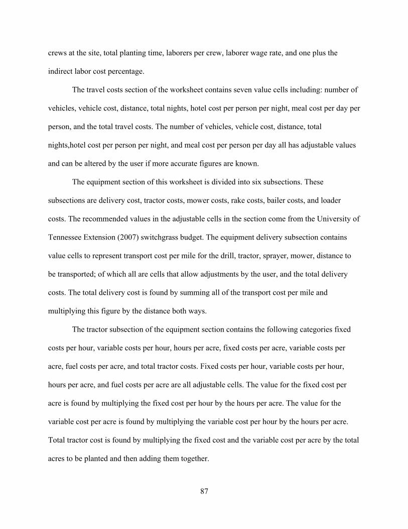
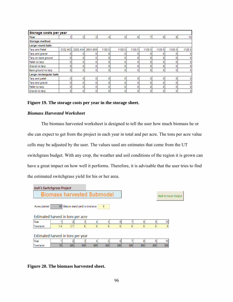
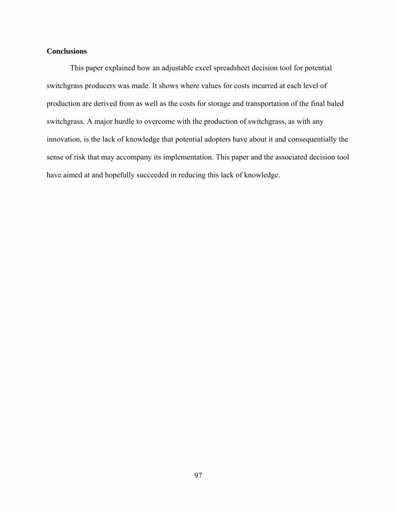
storage sheet .......................................................................................................................94 Figure 18. The dry matter loss schedule of the storage worksheet .....................................................95 Figure 19. The storage costs per year in the storage sheet ..................................................................96 Figure 20. The biomass harvested Sheet .............................................................................................96
Part 1: Introduction
2
Introduction
Much of the energy used in the industrialized world comes from fossil fuels such as coal,
petroleum, and natural gas. Although these chemicals are still being created underground by the
forces of heat and pressure, they are being consumed in quantities far exceeding the formation of
new reserves. This increased need for and scarcity of hydrocarbon energy pushes the search and
extraction of reserves toward more technically difficult deposits and less efficient forms of
hydrocarbon energy. The increased use of hydrocarbons also predicates the increased emission
of detrimental chemicals in our surrounding environment. For these reasons, there is a need to
find feasible sources of renewable energy that could prove to be more environmentally friendly.
One of these sources of renewable energy that has been the subject of much research is
biomass. Biomass is material derived from living or once living organisms such as herbaceous
and woody plant constituents and animal wastes that can be used to make solid, liquid, and
gaseous fuels. It is the largest source of renewable energy accounting for over 3 percent of the
energy consumed domestically and is also currently the only source for liquid renewable fuels
used in transportation (Perlack et al. 2005).
Of the possible ways to take advantage of direct and indirect energy from the sun,
biomass use is promising because it is compatible with current technologies and it can be stored
without technical problems which allows for its energy to be used when needed (Kaltschmitt
1994). Biomass could prove to be a clean energy source as it absorbs the carbon that it releases
during combustion from the atmosphere, potentially making it carbon neutral.
The source of biomass that will be the focus of this study is switchgrass. Switchgrass is a
C4 carbon fixation perennial warm season grass (Lewandowski et al. 2003). The perennial nature
of switchgrass gives it the advantage over annual crops for cellulosic biomass because it does not
3
have fixed annual establishment requirements. Its native habitat includes the prairies, open
ground and wooded areas, marshes, and pinewoods of much of North America east of the Rocky
Mountains and south of 55°N latitude (Stubbendieck et al. 1991). There are two distinct
geographic varieties or ecotypes of switchgrass: lowland and highland (Porter 1966; Brunken
and Estes 1975). Lowland types can be found on flood plains and other areas that may be subject
to inundation and upland types can typically be found in areas that have a low potential to flood
(Vogel 2004). Lowland types tend to be taller, coarser, and show the ability to grow more rapidly
than upland types (Vogel 2004).
There are many benefits that could be realized from the planting of switchgrass as a
biomass feedstock for fuel. Switchgrass has the capability to show high yields on soil that, due to
low availability of nutrients or water, would not lend itself to the cultivation of conventional
crops (Lewandowski et al. 2003). Being a native species, it also has a natural tolerance to pest
and diseases and can be grown successfully throughout a large portion of the United States with
minimal fertilizer applications (Jensen et al. 2007), which would be cost efficient and less
disruptive to the surrounding environment. Switchgrass has the capability to show high yields on
soil that, due to low availability of nutrients or water, would not lend itself to the cultivation of
conventional crops (Lewandowski et al. 2003), meaning that the grass could add profitability to
land that may not be economically useful otherwise. It has the positive attribute of reducing
erosion due to its extensive root system and canopy cover (Ellis 2006) and shows the potential
ability to reduce the buildup of CO2 by being a feedstock for a cleaner burning fuel than fossil
fuels and through soil carbon sequestration due it is being a deep rooted crop (Ma et al.2000).
Growing switchgrass as a biomass feedstock crop would add diversity to the American
crop mix. Introducing a new crop, like switchgrass, into a two crop rotation such as the corn-
4
soybean rotation that dominates the Corn Belt can help alleviate pest buildups that demand the
increased use of pesticides (Janick et al. 1996). Additionally, the introduction of new crops into
agricultural production can increase and protect farm income by diversifying farm products,
hedging risks, and expanding markets and can also act as a catalyst for rural economic
development by creating locally based processing and packaging industries (Janick et al. 1996).
Despite the potential benefits that could be realized from the planting of switchgrass,
there are significant obstacles to overcome. Several factors would have to be taken into
consideration before a bio-refinery that utilizes switchgrass to produce ethanol could be
established in a given area. Because of the high cost associated with the transportation of
biomass from switchgrass, the area from which a bio-refinery would feasibly be able to draw
feedstock would need to be small, preferably within a 30 mile radius (Mitchell, Vogel, and
Sarath 2008). This means that it would have to be determined if the local farmers would be
willing to devote sufficient acreage to switchgrass to meet the needs of the bio-refinery. This
willingness will be a function of numerous factors including biomass feedstock profits,
variability of profits, and correlation of profits relative to traditional crop profits (Larson et al.
2005).
The large scale production of switchgrass as a bio-energy feedstock is still in the
developmental stage. Consequently, a lack of an established market and of knowledge exists
both on the part of the producer pertaining to the costs and activities associated with its
production and on the part of the researcher pertaining to farmer’s willingness to produce and
attitudes toward switchgrass. While some studies have focused on factors that determine
farmers’ willingness to produce switchgrass and their general attitudes toward switchgrass and
its production (e.g. Jensen et al. 2007; Bransby 1998; Wen et al. 2005), these studies have been
5
limited in geographic scope and additional research is warranted that considers a broader
geographical area and different variables in order to gain a more complete understanding of how
producers view biomass feedstock production.
Knowledge of where switchgrass is likely to be adopted and the factors that are involved
in the producers’ decisions to adopt are of critical importance to understanding the potential
development of switchgrass as an energy feedstock at a market level. Additionally, with
switchgrass being a new crop, many producers may not be familiar with the production costs
associated with growing switchgrass. An understanding of these costs is crucial in the producers’
decisions of if and to what extent they would be willing to produce switchgrass. That stated, a
financial decision tool would be of assistance to producers in making these production decisions.
Objectives
The overall objectives of this study are: 1.) to analyze the willingness of producers in the
southeastern United States to plant switchgrass as a biofuel feedstock, 2.) to estimate the area of
switchgrass they would be willing to plant at different switchgrass prices, 3.) to evaluate the
factors that influence a producer’s decision to convert acreage to switchgrass, and 4.) to present a
spreadsheet-based decision tool for potential switchgrass producers.
This thesis is organized into two major sections. The first section is a paper that focuses
on the factors pertaining to farmers’ interest in planting switchgrass and those that are associated
with their likelihood and the extent to which they would be willing to produce switchgrass given
different plant gate prices. To accomplish this, a Tobit specification model with a binary sample
selection rule will be used. The binary sample selection rule will be used to analyze the
6
producers’ interests in growing switchgrass and the Tobit model is used to estimate acreage
adoption in response to switchgrass prices and other variables if the producer shows interest in
growing switchgrass.
The second section of this thesis is a paper that describes and documents an interactive
producer decision tool. This tool is an excel workbook that contains an intereactive switchgrass
budget. The tool provides the user with detailed information on the costs incurred in each stage
of a switchgrass operation in each year of its duration, which, for the purposes of this analysis,
will be 10 years. The decision tool is broken down into 13 different worksheets, including:
welcome worksheet
tutorial worksheet
input-output worksheet
cash flow worksheet
cost distribution worksheet
yearly cash flow worksheet
accumulated cash flow
planting and establishment worksheet
7
References
Bransby, D. I. “Interest Among Alabama Farmers in Growing Switchgrass for Energy.” 1998.
Paper presented at BioEnergy '98: Expanding Bioenergy Partnerships, MadisonWI, Oct.
4-8.
Brunken J.N., Estes J.R. 1975. “Cytological and morphological Variationin Panicum virgatum
L.”The Southwestern Naturalist 19(4):379–385
Ellis, P. 2006. “Evaluation of Socioeconomic Characteristics Of Farmers Who Choose to Adopt
a New Type of Crop and Factors That Influence the Decision to Adopt Switchgrass for
Energy Production.” M.S. Thesis, Department of Agricultural and Resource Economics.
Baidu-Forson, J. 1999. “Factors Influencing Adoption of Land-Enhancing Technology in the
Sahel: Lessons from a Case Study in Niger.” Agricultural Economics 20:231-239.
Bocqueho, G., and F. Jacquet. 2010. "The Adoption of Switchgrass and Miscanthus by Farmer:
Impact of Liquidity Constraints and Risk Preferences." Energy Policy 38(5): 2598-2607.
Bransby, D. I.1998. “Interest Among Alabama Farmers in Growing Switchgrass for
Energy.”Paper presented at BioEnergy '98: Expanding Bioenergy Partnerships,
MadisonWI, Oct. 4-8.
Bransby, D. I. 2005. "Switchgrass Profile". Bioenergy Feedstock Information Network
(BFIN),Oak Ridge National Laboratory.
Cho, S., S. Yen, J. Bowker, and D. Newman. 2008. “Modeling Willingness to Pay for Land
Conservation Easements: Treatment of Zero and Protest Bids and Application and Policy
Implications.” Journal of Agricultural and Applied Economics 40(1):267-285.
Daberkow, S. and W. McBride. 1998. “Socio-economic Profiles of Early Adopters of Precision
Agricultural Technologies.” Journal of Agribusiness 16(2):151-168.
Ellis, P. C. 2006 “Factors that Influence the Decision to Adopt Switchgrass for Energy
Production.” MS thesis, University of Tennessee, Knoxville.
Feder, G., R. E. Just, and D. Zilberman. 1985. “Adoption of Agricultural Innovations in
Developing Countries: A Survey.” Economic Development and Cultural Change
33(2):255-98.
42
Fernandez-Cornejo, J., D. Beach, and W. Huang. 1994. "The Adoption of IPM Techniques by
Vegetable Growers in Florida, Michigan and Texas," Journal of Agricultural andApplied
Economics 26(1): 158-172.
Fernandez-Cornejo, J., S. Daberkow, and W. D. McBride. 2001. “Decomposing the Size Effect
on the Adoption of Innovations: Agro-biotechnology and Precision Farming.” Paper
presented at the American Agricultural Economics Association Annual Meeting, Chicago,
IL. Aug. 5-8.
Fernandez-Cornejo, J., C. Hendricks, and A. Mishra. 2005. Technology Adoption and Off-farm
Income: The Case of Herbicide-Tolerant Soybeans. Journal of Agricultural and Applied
Economics 37(3): 549-563.
Hahn-Hagerdal B., M. Galbe, M. Gorwa-Grauslund, G. Liden, and G. Zacchi. 2006. Bio-ethanol:
the Fuel of Tomorrow from the Residues of Today.” Trends in Biotechnology 24:549-
556.
Hipple, P.C., and M.D. Duffy. 2002. “Farmer’s Motivation for Adoption of Switchgrass.” Trends
in New Crops and New Uses p.252-266.
Janick, J., M.G. Blase, D.L. Johnson, G.D. Joliffe, and R.L. Myers. 1996. Diversifying U.S. crop
production. P. 98-108. In: J. Janick (ed.), Progress in new crops. ASHS Press,
Alexandria, VA.
Jensen, K., C. D. Clark, P. Ellis, B. English, J. Menard,M. Walsh, and D. L. T. Ugarte. 2007.
“Farmer Willingness to Grow Switchgrass for Energy Production.” Biomass & Bioenergy
31:773-781.
Kaltschmitt, M. 1996. “The Benefits and Costs of Energy from Biomass in Germany”Biomass &
Bioenergy 6(5):329-337.
43
Kelsey, K. and T. Franke. 2009. “The Producers’ Stake in the Bioeconomy: A Survey of
Oklahoma Producers’ Knowledge and Willingness to Grow Dedicated Biofuel Crops.”
Journal of Extension 47(1):1-6.
Larson, J., B. English, and L. He. 2005. “Risk and Return for Bioenergy Crops under Alternative
Contracting Arrangements.” Paper presented at the Southern AgriculturalEconomics
Association Annual Meetings, Dallas TX, February 2-6.
Larson, J., B. English, C. Hellwinckel, D. Ugarte. 2005. “A Farmer Evaluation of Conditions
under Which Farmers Will Supply Biomass Feedstocks for Energy Production.” Paper
presented at the American Agricultural Economics Association Annual Meeting,
Providence RI, July 24-27.
Lewandski, I., J. M. O. Scurlock, E. Lindvall, and M. Chirstou. 2003. “The Development of
Perennial Rhizomatous Grasses as Energy Crops in the U. S. and Europe.” Biomass &
Bioenergy 25(4):335-361.
Lindner, R.K. 1987. “Adoption and Diffusion of Technology: an Overview.” In: Champ, B.R.,
E.Highly, J.V. Remenyi. “Technological Change in Postharvest Handling and
Transportation of Grains in the Humid Tropics.” ACIAR Proceedings Series, Australian
Centre for International Agricultural Research, 19:144-151.
Ma, Z., C. Wood, and D. Bransby. 2000. “Carbon Dynamics Subsequent to Switchgrass
Establishment.” Biomass and Bioenergy 18:93-104.
Marra, M., D. Pannell, and A. Ghadim. 2003. “The Economics of Risk, Uncertainty andLearning
in the Adoption of New Agricultural Technologies: Where are We on theLearning
Curve?” Agricultural Systems 75:215-234.
44
McLaughlin, S. B., and L. A. Kszos. 2005. “Development of Switchgrass (Panicum virgatum) as
a Bioenergy Feedstock in the United States.” Biomass & Bioenergy 28(6):515-535.
Mitchell, R., K. Vogel, and G. Sarath. 2008. “Managing and Enhancing Switchgrass as a Bio-
energy Feedstock.” Biofuels, Bioproducts, and Biorefining 2:530-539.
Nkonya E., T. Schroeder, and D. Norman. 1997. “Factors Affecting Adoption of Improved
Maize Seed and Fertilizer in Northern Tanzania.” Journal of Agricultural Economics
48:1-12.
Norris, P. E., and S. S. Batie. 1987. “Virgina Farmers’ Soil Conservation Decisions: an
Application of Tobit Analysis.” Southern Journal of Agricultural Economics 19:79-90.
Paulrud, S., and T. Laitila. 2010. “Farmers’ Attitudes about Growing Energy Crops: A Choice
Experiment Approach” Biomass and Bioenergy 34(12):1770-1779.
Perlack, R. D., L. L. Wright, A. F. Turhollow, L. R. Graham , B. J. Stokes, and D. C. Erbach.
2005. “Biomass as Feedstock for a Bioenergy and Bioproducts Industry: the Technical
Feasibility of a Billion-Ton Annual Supply.” U.S. Department of Agriculture and U. S.
Department of Energy, Oak Ridge TN, April.
Rajasekharan, P., and S. Veeraputhran. 2002. “Adoption of Intercropping in Rubber
Smallholdings in Kerala, India: a Tobit Analysis.” Agroforestry Systems 56:1-11.
Ransom J. K., K. Paudyal, and K. Adhikari. 2003. “Adoption of Improved Maize Varieties in the
Hills of Nepal.” Agricultural Economics23:299–305.
Sissine F. 2007. “Energy Independence and Security Act of 2007: A Summary of Major
Provisions” Congressional Research Service CRS report no. RL34294.
Stubbendieck, J., S. L. Hatch, and C. H. Butterfield. 1992. “North American Range Plants.”
Fourth edition. University ofNebraska Press, Lincoln, Nebraska, USA.
45
Velandia, M., D. Lambert, J. Fox, J. Walton, and E. Sanford. 2010. “Intent to Continue Growing
Switchgrass as a Dedicated Energy Crop: A Survey of Switchgrass Producers in East
Tennessee.” European Journal of Social Sciences 15(35):299-312.
Walton, J., J. Larson, R. Roberts, D. Lambert, B. English, S. Larkin, M. Marra, S. Martin, K.
Paton, and J. Reeves. 2010. “Factors Influencing Farmer Adoption of Portable Computers
for Site-specific Management: A Case for Cotton Production.” Journal of Agricultural &
Applied Economics 42(2): Forthcoming.
Wang, M. 2008. “Well-to-Wheels Energy and Greenhouse Gas Emission Results and Issues of
Fuel Ethanol.” Farm Foundation Agriculture and the Environment: Lifecycle Carbon
Footprint of Biofuels Workshop, January 29, 2008, Miami Beach, Florida.
Wen, Z., J. Ignosh, D. Parrish, J. Stowe, and B. Jones. 2005. “Identifying Farmers’ Interest in
Growing Switchgrass for Bio-energy in Southern Virginia.” Journal of Extension
47(4):5RIB7.
46
Appendix A: Tables
47
Table A.1. Farm and farmer demographics for the sample. Characteristics Census Averages Survey Respondent Percentages Net Farm Income Before Taxes Negative (Less than $0) $0 - $9,999 $10,000 - $14,999 $15,000 - $19,999 $20,000 - $24,999 $25,000 - $29,999 $30,000 - $34,999 $35,000 - $39,999 $40,000 - $44,999 $45,000 - $49,999 $50,000 - $74,999 $75,000 - $99,999 $100,000 - $149,999 At least $150,000 Net Off-farm Income Before Taxes Negative (Less than $0) $0 - $9,999 $10,000 - $14,999 $15,000 - $19,999 $20,000 - $24,999 $25,000 - $29,999 $30,000 - $34,999 $35,000 - $39,999 $40,000 - $44,999 $45,000 - $49,999 $50,000 - $74,999 $75,000 - $99,999 $100,000 - $149,999 At least $150,000 Education Level Obtained: Elementary/Middle school Some high school High school Some college College graduate Post graduate
Table A.2. Farm and farmer demographics for the sample cont. Characteristics Census Average Survey Respondent Percentages Total Acres: Acres owned Acres rented Acres rented to others Total acres farmed Age of Operator Farming Experience
318.82 acres - - -
58.0
-
Mean 240.59 acres 131.62 acres 194.68 acres 384.21 acres
60.28 years
35.3 years
49
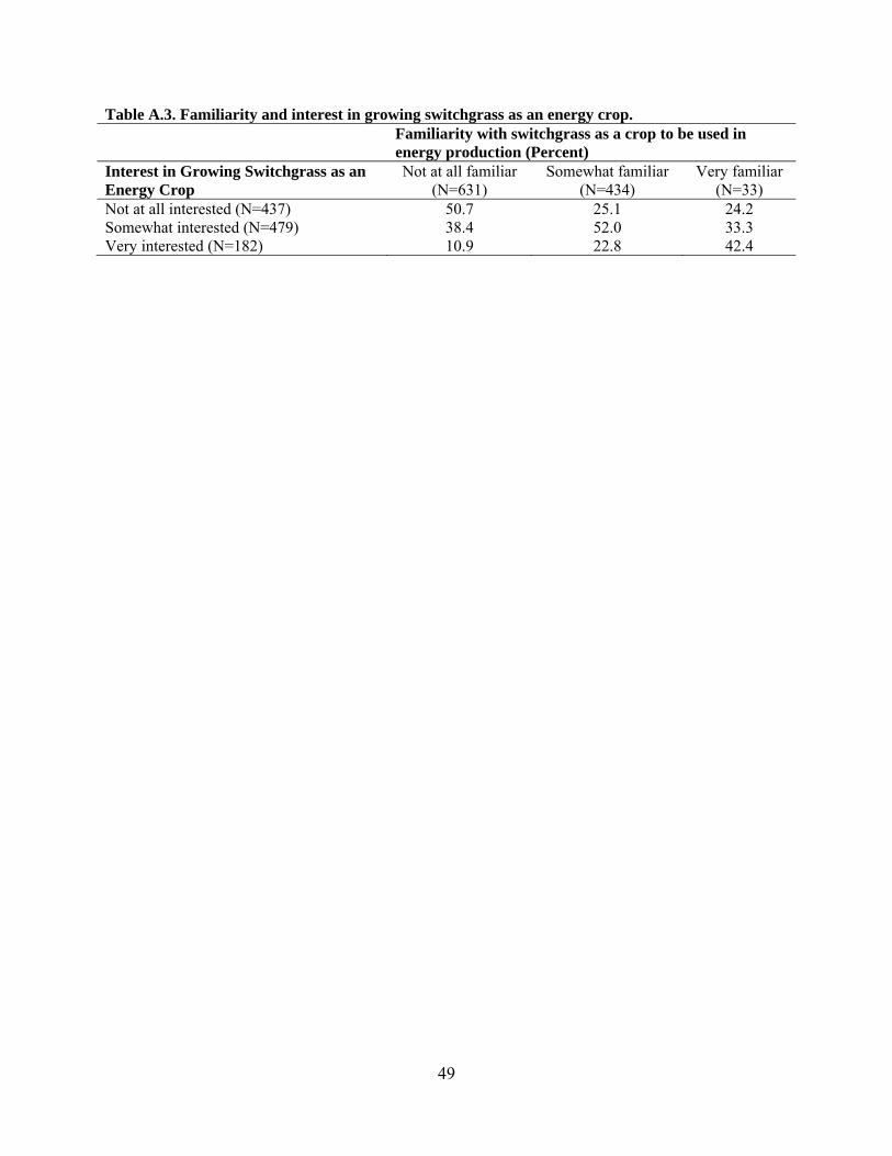
Table A.3. Familiarity and interest in growing switchgrass as an energy crop. Familiarity with switchgrass as a crop to be used in
energy production (Percent) Interest in Growing Switchgrass as an Energy Crop
Not at all familiar (N=631)
Somewhat familiar (N=434)
Very familiar (N=33)
Not at all interested (N=437) Somewhat interested (N=479) Very interested (N=182)
50.7 38.4 10.9
25.1 52.0 22.8
24.2 33.3 42.4
50
Table A.4. Farmer characteristics. Characteristic
All Survey Respondents
Not at all Interested Respondents
Somewhat Interested Respondents
Very Interested Respondents
Percent Owns a personal computer Extension workshops attended in 2008 Age Farming Experience Produced commodity under contract before Currently belongs to the following organizations : Grower/ commodity Cooperative Farm Bureau Hunting-related Environmental
74.22 (N=1253)
1.1 (avg. events)
(N=1195)
85 (N=1284)
60.3 (avg. years) (N=1241)
21.8
(N=1222)
13.9 (N=1169)
31.8
(N=1170) 57.7
(N=1172) 21.6
(N=1169) 8.7
(N=1169)
63.1 (N=471)
0.91(avg. events)
(N=485)
82 (N=468)
63.8 (avg. years) (N=504)
13.7
(N=497)
11 (N=483)
30.8
(N=483) 56.8
(N=484) 17.8
(N=483) 5.4
(N=483)
80.2 (N=531)
1.2 (avg. events)
(N=545)
87.2 (N=530)
58.6 (avg. years) (N=529)
25
(N=519)
13.2 (N=491)
32.3
(N=492) 57.4
(N=493 23
(N=491) 9.8
(N=491)
85.23 (N=210)
1.29 (avg. events)
(N=203)
87.5 (N=208)
56.3 ( avg. years) (N=208)
33
(N=206)
22.5 (N=195)
33.3
(N=195) 60.5
(N=197) 27.7
(N=195) 14.4
(N=195)
51
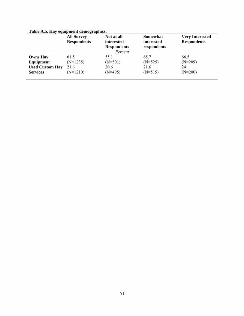
Table A.5. Hay equipment demographics. All Survey
Respondents Not at all interested Respondents
Somewhat interested respondents
Very Interested Respondents
Percent Owns Hay Equipment Used Custom Hay Services
61.5 (N=1235) 21.6 (N=1210)
55.1 (N=501) 20.6 (N=495)
65.7 (N=525) 21.6 (N=515)
66.5 (N=209) 24 (N=200)
52
TableA.6. Farmer concerns about risk and loss.
All Survey Respondents
Not at all interested Respondents
Somewhat interested respondents
Very Interested Respondents
Average responses from one to five with one being strongly disagree and 5 being strongly agree You are the type of farmer who is more willing to take financial risks than others You must be willing to take substantial financial risk to be a successful farmer You are reluctant about adopting new production methods or crops until you see them working for others You are more concerned about a large loss to your farming operation than about missing a substantial gain
Percent Description of farm operation Children or Grandchildren will inherit farm Land sold for development after farmer ceases Land will be sold or leased to other farmer after farmer ceases farming Other plans Livestock present on farm Farm Decisions Farm alone makes decisions Shared decision with partners or family Someone else makes the decisions Which best describes farm business Sole Proprietorship Partnership Cooperative Corporation Other
The symbol ‘***’ denotes significance at =.01, ‘**’ denotes significance at =.05, and ‘*’ denotes significance at =.10.
56
Appendix B: Survey
57
Switchgrass Production for Energy: Your Views
The purpose of this study is to collect information from farmers regarding their views on switchgrass production. Your participation in this study is completely voluntary. Your individual responses will be held confidential. Only summaries of the results will be presented. The survey should take you about 10 to 15 minutes to complete.
About Switchgrass
1.How familiar are you with switchgrass as a crop to be used in energy production? (Circle the answer)
Not at all familiar
(Skip to question 3)
Somewhat familiar
(Continue to question 2)
Very familiar
(Continue to question 2) 2.From which of the following sources have you obtained information on switchgrass?
(Check one box for each information source)
3.Please read through the following factors and circle how important each might be in influencing your decision to grow switchgrass (circle the number indicating the importance of each factor).
Factors Importance Level
Yes No
Farmer or commodity magazines Other mass media (Internet, radio, TV, newspapers, magazines) Extension Service University research stations or other university sources Federal agricultural agency (for example USDA, NRCS, FSA) State agricultural agency Farmer or commodity organizations Other farmers, friends, or neighbors Private firms Other (Please describe: _______________________________________)
58
Not at All Not Very
Some-what Very
Extre-mely
Possible conflicts between planting/harvest period for switchgrass and planting/harvest period for your other crops 1 2 3 4 5
Concern that the market for switchgrass as an energy crop is not developed enough yet 1 2 3 4 5
Profitability of growing switchgrass compared with other farming alternatives 1 2 3 4 5
Possibility that you will cease farming in the next few years due to retirement or other reasons 1 2 3 4 5
Your knowledge about growing switchgrass compared with your knowledge about growing other crops 1 2 3 4 5
Concern about planting a perennial crop such as switchgrass on land that is leased 1 2 3 4 5
Opportunity to diversify your farming operation 1 2 3 4 5
Potential for creating jobs in your community 1 2 3 4 5
Potential for switchgrass to reduce erosion on your farm 1 2 3 4 5
Whether acreage converted to switchgrass would qualify for CRP payments or not 1 2 3 4 5
Potential for switchgrass to provide habitat for native wildlife on your farm 1 2 3 4 5
Potential to contribute to national energy security by producing switchgrass for fuel 1 2 3 4 5
Potential to help the environment by producing switchgrass for fuel 1 2 3 4 5
Ability to use switchgrass as a feed for livestock 1 2 3 4 5
The three year lag between planting and switchgrass reaching its full yield potential 1 2 3 4 5
Possibility of lowering fertilizer and herbicide applications as compared with crops currently growing 1 2 3 4 5
Concern about having the financial and equipment resources needed to produce switchgrass 1 2 3 4 5
Other (Please describe: _________________________________________________________________ _____________________________________________________________________________________)
4. How interested are you in growing switchgrass as a crop to be used for energy production? (Circle the answer)
Not at all interested
Somewhat interested
Very interested
59
If you indicated you were NOT at all interested in growing switchgrass in question 4, please skip to question 12. If you indicated some interest in growing switchgrass in question 4, please continue on to question 5.
6. Would you be willing to sell at $70/ton if harvest services were provided?
Yes No, and the reason(s) are ________________________________
7.Would you prefer to grow switchgrass under a contract? (Check one box and fill in the blank)
Projected Yields for Switchgrass
Area Tons/ Acre
Alabama 5.1 Arkansas 5.1 Georgia 5.2 Kentucky 5.3 Louisiana 5.3 Mississippi 5.3 North Carolina 3.8 E. Oklahoma 4.5 W. Oklahoma 2.9 South Carolina 4.8 Tennessee 6.0 E. Texas 3.9 Western Texas 3.7 Virginia 4.9
5. Annual switchgrass yields in your area are listed in the table to the left. Assume you are responsible for harvesting costs and all inputs, except seed, which is provided by the contractor.
Would you be willing to sell switchgrass at a price of $100/ton if the switchgrass is picked up at your farm at the time of harvest? (Check one box and fill in the blank)
No, and the reason(s) are ______________________ _________________________________________
Yes
and I would be willing to produce ________ acres
What are the current uses of the land you would convert (for example type of crop, pasture, idle, CRP, timber, or other)? If some of the land would be newly rented land, please list as “new rented acres”.
Type of crop or other use (ex: pasture, idle, CRP, forest, etc.)
Number of acres to be converted
a. _____________________________________________________ _______________
b. _____________________________________________________ _______________
c. _____________________________________________________ _______________
d. _____________________________________________________ _______________
e. ____________________________________________________ _______________
Total acres converted to switchgrass =
_______________
60
Yes, and the contract length would need to be _______ years No
8. If you were to grow switchgrass, would you be willing to store it on your farm after harvest if you were reasonably compensated for the costs? (Check one box)
Yes No, and the reason(s) are ________________________________ ______________________________________________________ (Skip to question 11)
9. If you were willing to store switchgrass on your farm, and the switchgrass was harvested in December, how long would you be willing to store it? _______ days
11.Would you be interested in participating in a cooperative that harvests,
transports, stores, and markets switchgrass? (Check one box)
Yes No, and the reason(s) are ___________________________________
About Your Farming Operation
12. How many acres did you farm in 2008 that you (Fill in the blanks):
Owned ________ acres Rented ________ acres (rent paid was $_______/acre and the lease was for _____ years) Other ________ acres (farmed but neither owned nor rented these acres)
10. Which best describes your storage situation (Check one box)
You have an existing hay shed or barn where the switchgrass could be stored
You can store about _______ number bales of hay in this barn. Indicate bale type with a check mark.
_______ large square
_______ small square _______ large round _______ other
You would construct storage facilities (such as a gravel pad with tarp for cover)
Other (Please describe:______________________________________________)
61
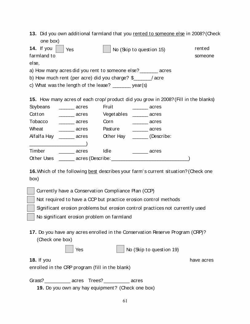
13. Did you own additional farmland that you rented to someone else in 2008? (Check
one box)
14. If you rented
farmland to someone
else,
a) How many acres did you rent to someone else? _______ acres
b) How much rent (per acre) did you charge? $_______/acre
c) What was the length of the lease? _______ year(s)
15. How many acres of each crop/product did you grow in 2008? (Fill in the blanks)
Soybeans ______ acres Fruit ______ acres
Cotton ______ acres Vegetables ______ acres
Tobacco ______ acres Corn ______ acres
Wheat ______ acres Pasture ______ acres
Alfalfa Hay ______ acres Other Hay ______ (Describe:
______________________)
Timber ______ acres Idle ______ acres
Other Uses ______ acres (Describe:______________________________)
16.Which of the following best describes your farm’s current situation? (Check one
box) Currently have a Conservation Compliance Plan (CCP) Not required to have a CCP but practice erosion control methods
Significant erosion problems but erosion control practices not currently used No significant erosion problem on farmland
17. Do you have any acres enrolled in the Conservation Reserve Program (CRP)?
(Check one box)
18. If you have acres
enrolled in the CRP program (fill in the blank)
Grass? __________ acres Trees? __________ acres
19. Do you own any hay equipment? (Check one box)
Yes No (Skip to question 15)
Yes No (Skip to question 19)
62
20.What types of hay equipment do you own? (For each type of equipment, check one
box, then fill in the blanks)
21. Did you use custom hay harvest services in 2008? (Check one box)
22. If you used custom hay harvest services in 2008, indicate the costs per acre.(Fill
in the blanks)
Mowing/raking $_________/acre Baling for small square bales $_________/bale
Baling for round bales $_________/bale Baling for large square bales $_________/bale
23. Do you currently use no-till production methods? (Check one box) 24. Do you have any of the following types of livestock operations? (For each type of
livestock operation, check one box) Yes No Yes No
Beef cow-calf Hogs
Backgrounding/stockering Horses Dairy cattle Other (Please describe: _______________ Poultry ________________________________________)
25. Which of the following best describes your farming operation? (Check one box)
One or more of your children or grandchildren will farm your land after you
Your land will be sold for development after you cease farming
Yes No (Skip to question 21)
Yes No Mower
Rake Round Baler bale size_____________________ Small Square Baler bale size_____________________ Large Square Baler bale size_____________________ Other (Please describe: _____________________________________)
Yes No (Skip to question 23)
Yes No
63
Your land will be sold or leased to another farmer after you cease farming
Other (Please describe: _________________________________________)
26. Which of the following best describes your role in deciding which crops to grow on your farm? (Check one box)
I make the decision on my own
I share the decision making with partners or family
Someone else makes this decision
27. Which of the following best describes your farming business? (Check one box)
Sole proprietorship
A partnership
A cooperative
A corporation
Other (Please describe: _________________________________________)
28. Which of the following describes your farming operation’s net income from
farming in 2008 (before taxes)?(Check one box)
29.For every $100 of farm assets your farming operation has, how many dollars are financed with debt? (Check one box)
$0 $5-$9.99 $15-$19.99 $40-$69.99
$1-$4.99 $10-$14.99 $20-$39.99 greater than $70
30.Have you ever produced any commodity under contract? (Check one box)
Negative (less than $0) $25,000-$29,999 $50,000-$74,999
$0-$9,999 $30,000-$34,999 $75,000-$99,999
$10,000-$14,999 $35,000-$39,999 $100,000-$149,999
$15,000-$19,999 $40,000-44,999 At least $150,000
$20,000-$24,999 $45,000-49,999
Yes No
64
About You
31.Your age in years__________ Your years of experience farming _________ 32.Do you own a personal computer?(Check one box) 33.How many extension workshops or experiment station field days did you attend in
2008? (Fill in the blank) ________ 34.What is the highest education level you have attained? (Check one box)
35.What was your household’s 2008 net income (before taxes) from off-farm sources?
36. Please circle the answers that reflect your level of agreement with each of the following statements.
Statement Strongly Disagree Disagree
No Opinion Agree
Strongly Agree
You are the kind of farmer who is more willing to take financial risks than others
1 2 3 4 5
You must be willing to take substantial financial risks to be a successful farmer
1 2 3 4 5
You are reluctant about adopting new production methods or crops until you see them working for others
1 2 3 4 5
You are more concerned about a large loss to your farming operation than about missing a substantial gain
1 2 3 4 5
Yes No
Elementary/Middle school High school College graduate
Some high school Some College Post graduate
Negative (less than $0) $25,000-$29,999 $50,000-$74,999
$0-$9,999 $30,000-$34,999 $75,000-$99,999
$10,000-$14,999 $35,000-$39,999 $100,000-$149,999
$15,000-$19,999 $40,000-44,999 At least $150,000
$20,000-$24,999 $45,000-49,999
65
Part 3: AN EXCEL SPREADSHEET-BASED DECISION TOOL FOR POTIENTIAL
SWITHGRASS PRODUCERS
66
Introduction
Due to factors such as dependence on foreign oil and environmental concerns, there have
been government policy initiatives dealing with alternative fuels that have far reaching impacts
on the United States and world economies. An example of this type of policy is the Energy
Independence and Security Act (EISA) of 2007, with its key provision being the Renewable Fuel
Standard (RFS). The RFS has generated increased research into biomass production by
mandating that by at least 36 billion gallons of ethanol for fuel be produced in the United States
by 2022, with at least 16 billion gallons being ethanol that is derived from cellulose, hemi-
cellulose, or lignin (U.S. Congress 2007).
Biomass accounts for over 3 percent of the energy consumed domestically and is
currently the only source for liquid renewable fuels used in transportation (Perlack et al. 2005).
There are many sources of biomass that can be used to make solid, liquid, and gaseous fuels
including woody plants and their associated manufacturing waste and residues, aquatic plants,
biological waste, and herbaceous plants such as grasses (Mckendry 2001). Biomass is promising
because it allows us to take advantage of energy from the sun in a way that is compatible with
current technologies and can be stored without technical problems allowing its energy to be used
when needed and it could prove to be a clean energy source as the carbon that it releases during
combustion is obtained from the atmosphere, potentially making it carbon neutral.
Generating sufficient biomass to meet the EISA’s 16 billion gallon cellulosic ethanol
quota will require the production of dedicated energy crops. Switchgrass (Panicum virgatum) is
among the species of herbaceous plants being considered to help meet the expected demand
generated for biomass. Switchgrass is a warm season perennial grass. The perennial nature of
67
switchgrass separates it from more conventional annual crops because it does not have fixed
annual establishment requirements. Its native habitat includes the prairies, open ground and
wooded areas, marshes, and pinewoods of much of North America east of the Rocky Mountains
(Stubbendieck et al. 1991). There are two distinct geographic varieties or ecotypes of
switchgrass, lowland and highland (Porter 1966; Brunken and Estes 1975). Lowland types can be
found on flood plains and other areas that may be subject to flooding and upland types can
typically be found in areas that have a low potential to flood (Vogel 2004). Lowland types tend
to be taller, coarser, and show the ability to grow more rapidly than upland types (Vogel 2004).
Many benefits could be seen through the planting of switchgrass as a biomass feedstock
for fuel. Because it is a native species, it also has a natural tolerance to pest and diseases and can
be grown successfully throughout a large portion of the United States with minimal fertilizer
applications (Jensen et al. 2007), which would be cost efficient and less disruptive to the
surrounding environment. Switchgrass has the capability to show high yields on soil that, due to
low availability of nutrients or water, would not lend itself to the cultivation of conventional
crops (Lewandowski et al. 2003) which means that the grass could add utility to land that may
not be economically useful otherwise. It has the positive attribute of reducing erosion due to its
extensive root system and canopy cover (Ellis 2006) and shows the potential ability to reduce the
buildup of CO2 by being a feedstock for a cleaner burning fuel than fossil fuels and through soil
carbon sequestration due it is being a deep rooted crop (Ma et al.2000).
Despite these possible benefits that could be realized from the implementation of
switchgrass as a dedicated energy crop, there are hurdles to overcome. One of the draw backs
associated with switchgrass being produced for biomass used in energy production, being an
innovative practice, is that there is unfamiliarity associated with the specific costs of its
68
production. The decision of a farmer to adopt an innovation is based on its perceived ability to
provide more utility than other viable options which may be more conventional and whose
associated risk may be more known and understood. Because of this, the distribution of
knowledge related to the innovation, which for this study is the costs associated with the
production of switchgrass, becomes imperative to the adoption of the practice. A productive way
to disseminate this information in a manner that is readily understandable and adjustable to fit
each individual farmer’s operation is to apply it to a production decision tool in an excel
workbook.
Objective
The objective of this paper is to explicate and present an interactive and adjustable excel
spreadsheet-based decision tool for potential switchgrass producers that provides the user with
detailed information on the costs incurred in each stage of a switchgrass operation in each year of
its duration, which, for the purposes of this analysis, will be 10 years. The budget workbook is
broken down into 13 different worksheets, including:
welcome worksheet
tutorial worksheet
input-output worksheet
cash flow worksheet
cost distribution worksheet
yearly cash flow worksheet
accumulated cash flow
planting and establishment worksheet
69
stand maintenance worksheet
harvest worksheet
transportation worksheet
storage worksheet
biomass harvested worksheet
In the following chapters, the purpose of each worksheet, the source of the estimated figures in
their adjustable cells, and the methods used in their calculating cells will be explained.
Literature Review
A significant portion of literature relating to switchgrass concerns the economic aspects
of its production and delivery to a bio-refinery for the purpose of creating bio-energy. Many of
these studies are regionally (e.g. Cundiff and Marsh 1996; Epplin 1996; Larson et al. 2010a;
Larson et. al 2010b) or state (e.g. Sladden, Bransby, and Aiken 1991; Popp 2007) specific due to
the variation in suitability of the crop and the focus on biomass production for alternative fuels in
the area. Other studies focus on analyzing the cost of using switchgrass as a cellulosic biomass
feedstock in comparison to other possible grass species options (e.g. Haque et al. 2008; Wilkes
2007). The results from these studies and others like them provide information used to compose
budgets like those that create the foundation of this study.
Larson et al. (2010a), Larson et al. (2010b), Wang et al. (2009a), and Wang et al. (2009b)
are examples of studies that consider the storage cost, among other costs, and biomass losses for
different periods of storage time and methods. The data used in these studies came from a
switchgrass harvest and storage study at the Milan Research and Education Center in Milan,
Tennessee (English et al. 2008). The study analyzed many different storage options including
whether the bails were round or square, if they were placed on bare ground or on a wooden
70
pallet, the amount of time the bales were stored, and whether or not the bales were covered with
a tarp. This data has been eminently valuable to this study by providing a base useable to
calculate an estimate of the cost of storage given the type of bale used and the storage method as
well as the loss in biomass given the duration of storage.
Fulton (2010) is a study that evaluated the impacts that introducing cellulosic ethanol
plants in east Tennessee and west Tennessee would have on the economies of these two regions.
In doing this, the study analyzed the costs of transporting the switchgrass from the farm to the
bio-refinery. This information has been valuable in assembling the transportation cost section of
this study.
The Woody Biomass Program ran by the College of Environmental Science and Forestry
(ESF) at the State University of New York (SUNY) in 2008 created a Microsoft Excel based
production decision tool for growing willow (Genus: Salix) for biomass energy production called
“EcoWillow”. This willow decision tool assumed planting on marginal soils with low labor,
machinery, fertilizer, and herbicide inputs compared to traditional crops. It details the costs
associated with willow establishment, stand maintenance, harvesting, and the transportation of
the biomass. It can have a stand life of 11 or 22 years, depending on which the user chooses.
While it is useful in determining total cost estimates, it lacks the ability to estimate the cost of
storage and the amount of biomass dry matter loss during storage, both of which can factor
prominently in estimating whether or not a switchgrass stand will be a fortuitous endeavor.
Bransby et al. (2005) is a study that used Microsoft Excel to model a switchgrass budget.
It allowed for alternative producing, harvesting, handling, and transporting methods. Similar to
the Eco-Willow program created by the Woody Biomass Program at SUNY, it lacks the ability
to calculate and account for the cost of and dry matter loss during storage.
71
For any business activity, an estimated budget is needed before it is started and there are
multiple examples of budgets dealing with switchgrass operations (Wilkes 2007; Green and
Benson 2008; UT Extension 2009; UT Extension 2007). Green and Benson (2008) is a budget
put together at North Carolina State University that gives the same values for the revenues and
costs for each year of a switchgrass project. It mentions all important costs but lacks specificity
with some of the more detailed expenses. Wilkes (2007) is a budget made for the Natural
Resources Conservation Service Plant Materials Program. It estimates different costs associated
with the establishment and subsequent years, with the subsequent years having the same costs
projections. Because it covers three other grass budgets, it was not a relatively in depth analysis
of switchgrass. The University of Tennessee Extension budget (2007) and (2009) serve as
guidelines for establishing a switchgrass stand and up to ten years afterward. Most of the
recommended values for input cost in this study have been drawn from these budgets.
Case Study
For illustrative purposes, the figures in this study will represent a specific case. This case
will assume a 50 acre switchgrass stand with a mature yield of 6 dry tons of biomass per acre and
that the producer will receive 75 dollars per dry ton at the plant gate. The biomass will be stored
on farm for 200 days as round bales on pallets covered with a tarp. All other values to be used
for the case study will be the suggested University of Tennessee Extension Budget values.
Methods
Input – Output Sheet
The input-output worksheet is the most integral worksheet in this excel workbook. It ties
together the values from all of the other sheets in a way that is understandable to the user and has
macros buttons that direct the user to each respective page. The two input sections of the
72
worksheet are general data and startup loans. The output sections are financial analysis tools,
production costs, and revenues and earnings.
Input Section
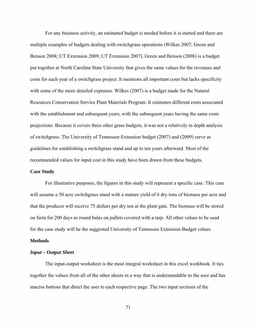
The general data section (Figure 1.) has six cells where the user can insert specific data.
The interest rate for this workbook is determined in this section. The suggested interest rate is the
current thirty year Treasury bond; however, the user has the ability to input any desired rate, as
interest rates tend to fluctuate daily.
In this section, the user can input the cost of land, which includes taxes, leasing fees, and
insurance. Internal administration fees are to be included in this section, as well. There are cells
in this section that allow the user to include total acreage incentive payments they may receive
from government agencies or any other organization and their duration. The last cell in this
section gives the user the ability to insert the current price per dry ton of switchgrass at the plant
gate. The suggested price per ton is $75.00 USD.
The startup loan section (Figure 1.) contains information regarding any loans that are
taken out to establish the switchgrass stand. The three pieces of information to input are available
equity, the amount of the loan, and the interest rate. This information will be used to determine
the loan payments per period, assuming the loan is paid off over the life of the project which, in
this case, is 10 years as according to Qin et al. (2006).
73
Figure 1. The input section of the input-output sheet.
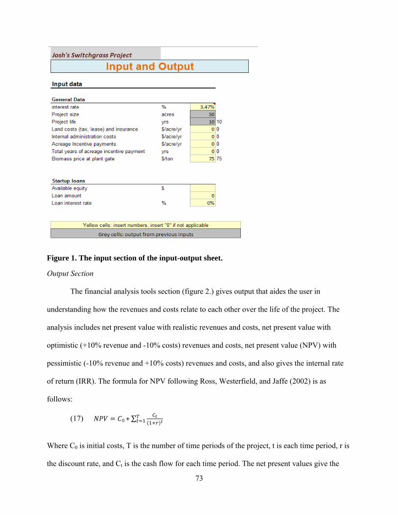
Output Section
The financial analysis tools section (figure 2.) gives output that aides the user in
understanding how the revenues and costs relate to each other over the life of the project. The
analysis includes net present value with realistic revenues and costs, net present value with
optimistic (+10% revenue and -10% costs) revenues and costs, net present value (NPV) with
pessimistic (-10% revenue and +10% costs) revenues and costs, and also gives the internal rate
of return (IRR). The formula for NPV following Ross, Westerfield, and Jaffe (2002) is as
follows:
(17) 0 + ∑
Where C0 is initial costs, T is the number of time periods of the project, t is each time period, r is
the discount rate, and Ct is the cash flow for each time period. The net present values give the
74
user an idea as to what the investment is worth in current terms after discounting each year’s
earnings back to the current period given that the project could go as planned, better than
planned, or worse than planned. The IRR is the r where
(18) 0 + ∑ = 0.
Basically, the IRR is the rate of return of a project where the NPV of the project is equal to zero.
The production costs, revenues, and earnings section (Figure 2.), like the financial
analysis tools section, is meant to aid the user in understanding the revenues and costs associated
with the project. This section contains average costs per acre, average gross revenue per acre,
average profit per acre, average revenue per ton, average costs per ton, and average earning per
ton. All of these reflect the average values over the total life of the project.
Figure 2. The output section of the input-output sheet.
75
Cash Flow Sheet
The cash flow worksheet documents the revenues and the expenditures for each year over
the life of the operation. It shows the total and per acre and per acre revenues and expenditures in
two separate diagrams. The expenditures per year include the following categories: land cost and
insurance, administration cost, planting and establishment cost, storage cost, stand maintenance
cost, harvest cost, and transportation cost. Planting and establishment costs apply only to the first
year of the project while stand maintenance, which includes the cost of reseeding applies to years
2 through 9. Included in the revenues section is the amount of money received for the biomass
and any sort of acreage incentive payments that the user might stand to receive. Finally,
expenditures are subtracted from revenues to calculate profit before the subtraction of loans,