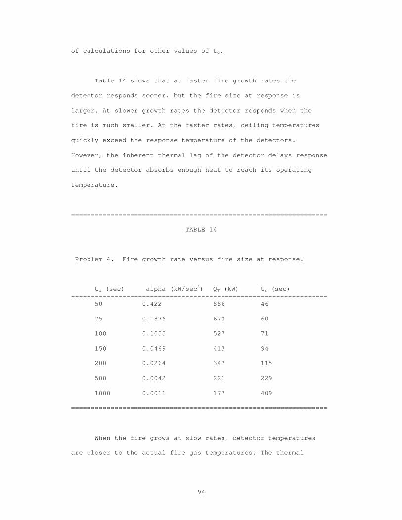
i USE OF FIRE PLUME THEORY IN THE DESIGN AND ANALYSIS OF FIRE DETECTOR AND SPRINKLER RESPONSE by Robert P. Schifiliti A Thesis Submitted to the Faculty of the WORCESTER POLYTECHNIC INSTITUTE in partial fulfillment of the requirements for the Degree of Master of Science in Fire Protection Engineering January 1986 APPROVED: (Signed) Prof. Richard L. Custer, Major Advisor (Signed) Dr. Craig L. Beyler, Associate Advisor (Signed) Prof. David A. Lucht, Head of Department
Transcript
i
USE OF FIRE PLUME THEORY IN THE DESIGN AND
ANALYSIS OF FIRE DETECTOR AND SPRINKLER RESPONSE
byRobert P. Schifiliti
A Thesis
Submitted to the Faculty
of the
WORCESTER POLYTECHNIC INSTITUTE
in partial fulfillment of the requirements for the
Degree of Master of Science
in
Fire Protection Engineering
January 1986
APPROVED:
(Signed)
Prof. Richard L. Custer, Major Advisor
(Signed)
Dr. Craig L. Beyler, Associate Advisor
(Signed)
Prof. David A. Lucht, Head of Department
Notice of Disclaimer
This thesis references and uses correlations developed by Heskestad and Delichatsios for
ceiling jet temperature and velocity from t2 fires.
The correlations by Heskestad and Delichatsios were developed assuming that the test
fuel had a heat of combustion of 20,900 kJ/kg and a convective heat release fraction of
about 75%. Subsequently, experimentation showed that a heat of combustion equal to
12,500 kJ/kg would be a more accurate value for the wood cribs used in the test.
Heskestad and Delichatsios subsequently published updated correlations based on this
new value. Consequently, the correlations in this thesis are incorrect.
The correlations for t2 fires were developed using data from a series of wood crib burn
tests. The test fires had a convective heat release fraction of approximately 75%.
Modeling fuels having different convective fractions will produce some degree of error.
In their updated paper, Heskestad and Delichatsios also provided correlations based only
on the convective heat release rate. These correlations should be used when the
convective fraction is significantly different than the 75% from the original test series.
The following references discuss these changes and their effects in more detail. They
also discuss how correction factors can be applied to computer programs or models that
use the older, incorrect correlations in order to adjust for the inherent error.
G. Heskestad and M. Delichatsios, “Update: The Initial Convective Flow in Fire”, Fire Safety Journal, Volume 15, 1989, p. 471-475. R.P. Schifiliti and W.E. Pucci, Fire Detection Modeling: State of the Art, the Fire Detection Institute, Bloomfield, CT, 1996. NFPA 72, National Fire Alarm Code, National Fire Protection Association, Quincy, MA 1999.
- R.P. Schifiliti, March 31, 2000
ii
ABSTRACT
This thesis demonstrates how the response of fire detection
and automatic sprinkler systems can be designed or analyzed. The
intended audience is engineers involved in the design and
analysis of fire detection and suppression systems. The material
presented may also be of interest to engineers and researchers
involved in related fields.
National Bureau of Standards furniture calorimeter test
data is compared to heat release rates predicted by a power-law
fire growth model. A model for calculating fire gas temperatures
and velocities along a ceiling, resulting from power-law fires is
reviewed. Numerical and analytical solutions to the model are
outlined and discussed.
Computer programs are included to design and analyze the
response of detectors and sprinklers. A program is also included
to generate tables which can be used for design and analysis, in
lieu of a computer.
Examples show how fire protection engineers can use the
techniques presented. The examples show how systems can be
designed to meet specific goals. They also show how to analyze a
system to determine if its response meets established goals. The
examples demonstrate how detector response is sensitive to the
detector's environment and physical characteristics.
iii
ACKNOWLEDGEMENTS
I would like to thank Dick Custer, Jonathan Barnett and
Craig Beyler for their help and advice which led to the
conclusion of this thesis. I must also express my gratitude to
Dr. Fitzgerald for his many years of guidance and to Wayne Moore
for his continued support and friendship.
Most of all I thank my wife, Chris, for her love and
understanding, without which I could not have completed this
work.
iv
TABLE OF CONTENTS
ABSTRACT -------------------------------------------- ii
ACKNOWLEDGEMENTS ------------------------------------ iii
LIST OF TABLES -------------------------------------- vi
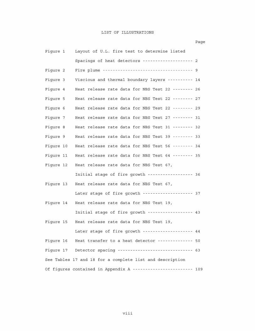
LIST OF ILLUSTRATIONS ------------------------------- viii
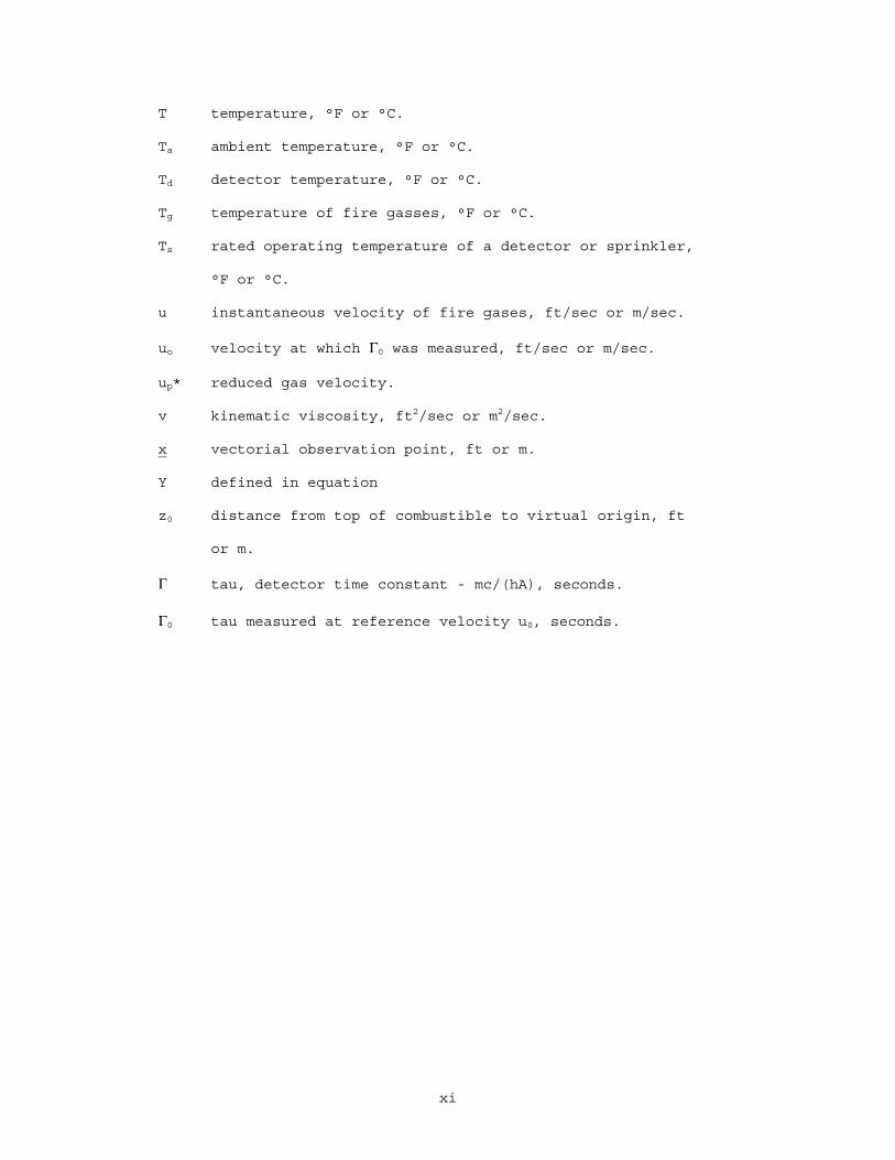
NOMENCLATURE ---------------------------------------- ix
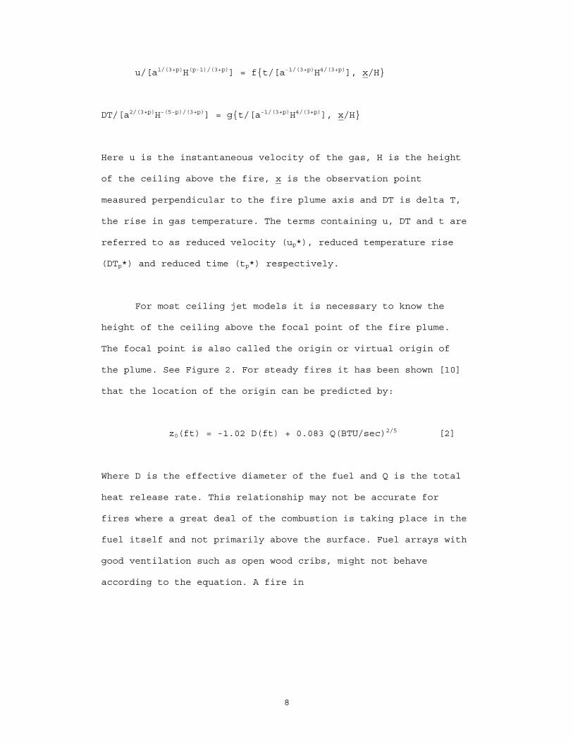
Here u is the instantaneous velocity of the gas, H is the height
of the ceiling above the fire, x is the observation point
measured perpendicular to the fire plume axis and DT is delta T,
the rise in gas temperature. The terms containing u, DT and t are
referred to as reduced velocity (up*), reduced temperature rise
(DTp*) and reduced time (tp*) respectively.
For most ceiling jet models it is necessary to know the
height of the ceiling above the focal point of the fire plume.
The focal point is also called the origin or virtual origin of
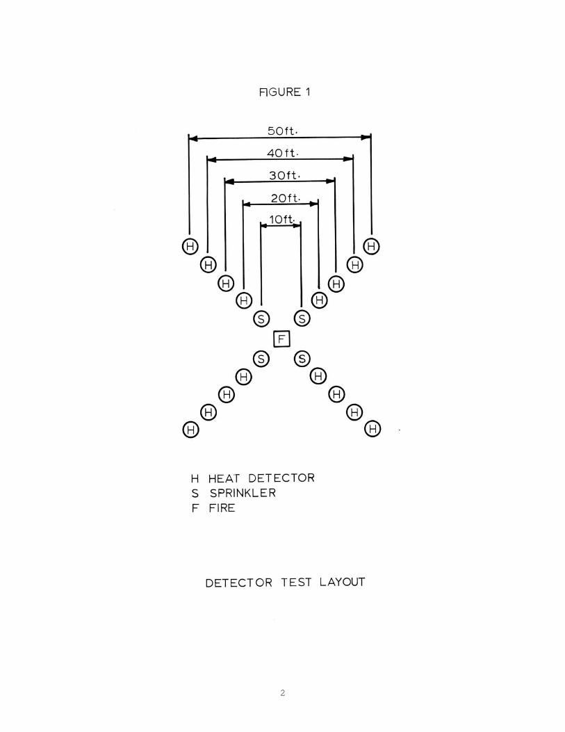
the plume. See Figure 2. For steady fires it has been shown [10]
that the location of the origin can be predicted by:
z0(ft) = -1.02 D(ft) + 0.083 Q(BTU/sec)2/5 [2]
Where D is the effective diameter of the fuel and Q is the total
heat release rate. This relationship may not be accurate for
fires where a great deal of the combustion is taking place in the
fuel itself and not primarily above the surface. Fuel arrays with
good ventilation such as open wood cribs, might not behave
according to the equation. A fire in
9
10
a well ventilated wood crib will have a substantial amount of
combustion taking place inside the crib, below the surface.
Heskestad and Delichatsios [6] chose to use the height
above the fuel surface H, in their work. Later, the effects of
this assumption will be tested by comparing results obtained
using the height above the fuel surface, H, to results using the
height above the virtual origin, H0.
In analyzing test data it was found that many fires closely
follow the power-law growth model with p = 2 [6]. The functional
relationships then take the form:
u2* = f (t2*, r/H)
DT2* = g (t2*, r/H)
Here r is the radial distance from the fire.
For convenience Heskestad and Delichatsios define the
critical time, tc, by the following relationship:
a = 1000 (BTU/sec) / [tc(sec)]2 [3]
or:
tc = [1000 (BTU/sec) / a]1/2 [4]
The critical time is the time at which the fire would reach a
11
heat output of 1000 BTU/sec. Heskestad and Delichatsios used tc
(in lieu of a) to describe the rate of fire growth in the
formulas they present. The word critical may be misleading as tc
does not represent any particularly important event in the growth
of a fire. tc is merely used for convenience in place of alpha.
Heskestad and Delichatsios found the following
relationships to agree closely with data collected in the test
series [6]
t = (0.251 tc2/5H4/5) t2* [5]
DT = (15.8 tc-4/5H-3/5) DT2* [6]
u = (3.98 tc-2/5H1/5) u2* [7]
and:
t2f* = 0.75 + 0.78(r/H) [8]
If t2* < t2f* then: DT2* = 0
Else:
If t2* > t2f* then:
t2*=0.75+2.22(DT2*/1000)0.781+
[0.78+3.69(DT2*/1000)0.870](r/H) [9]
u2*/(DT2*1/4)=0.36(r/H)-0.315 [10]
12
Here t2f* is the reduced arrival time of the heat front at the
detector location. Equation 8 is used with Equation 5 to
calculate the actual time when the heat front reaches the
detector.
By rearranging the terms, Equation 9 is expressed in terms
of t2f*
t2*=t2f*+2.22(DT2*/1000)0.781+
3.69(DT2*/1000)0.870(r/H) [11]
The data show these relationships cease to be valid at
temperatures of about 1600 degrees F along the axis of the fire
plume [6]. The equations assume open flaming combustion is
established and the fire obeys the power-law growth model with p
= 2.
The equations do not model smoldering combustion. This is
because during smoldering, most of the heat being released by the
combustion process is being absorbed by the fuel itself. This
heat liberates additional volatiles from the fuel. These
equations are used only when sufficient volatiles are being
driven from the fuel and are reacting in a combustion zone above
the fuel surface. In addition, a sufficient amount of the heat
being released in the combustion zone must be carried away from
the fuel in a rising convective plume.
13
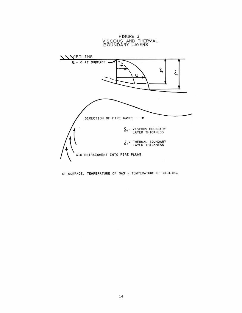
When any fluid flows across a flat plate such as a ceiling,
the velocity of the fluid immediately adjacent to the plate is
zero. Moving away from the ceiling the flow increases to full
flow. This is shown graphically in Figure 3. Within the small
boundary layer, the effects of ceiling drag and heat transfer to
the ceiling can not be neglected. The thickness of this boundary
layer is a function of the velocity and the kinematic viscosity
of the fire gases.
Detectors, thermocouples and velocity probes used in the
tests at Factory Mutual were located four and one half to five
inches below the ceiling. Based on model calculations, Beyler [7]
concludes that these measurements were taken outside of the
viscous boundary layer, which he estimated to be a maximum of
three inches in the tests. Hence the similarity equations
proposed by Heskestad are used to model the flow and temperature
of fire gases outside of the boundary layer.
The value of these relationships is that they can be used
to calculate the gas temperature and velocity in the vicinity of
the ceiling at some distance r, from the fire. These calculations
are at time t, for a fire with a growth characteristic alpha, or
a critical time tc and at some position r and H. In this form the
equations are solved numerically for the fire gas temperature and
velocity.
14
15
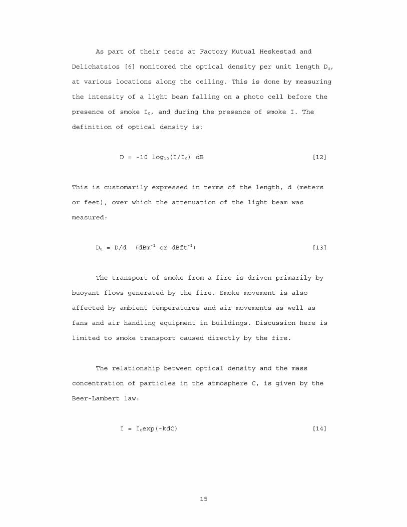
As part of their tests at Factory Mutual Heskestad and
Delichatsios [6] monitored the optical density per unit length Du,
at various locations along the ceiling. This is done by measuring
the intensity of a light beam falling on a photo cell before the
presence of smoke I0, and during the presence of smoke I. The
definition of optical density is:
D = -10 log10(I/I0) dB [12]
This is customarily expressed in terms of the length, d (meters
or feet), over which the attenuation of the light beam was
measured:
Du = D/d (dBm-1 or dBft-1) [13]
The transport of smoke from a fire is driven primarily by
buoyant flows generated by the fire. Smoke movement is also
affected by ambient temperatures and air movements as well as
fans and air handling equipment in buildings. Discussion here is
limited to smoke transport caused directly by the fire.
The relationship between optical density and the mass
concentration of particles in the atmosphere C, is given by the
Beer-Lambert law:
I = I0exp(-kdC) [14]
16
where k is the absorption coefficient of the smoke. It has been
shown [11] that k is dependent on the particle size distribution
of the smoke. However, if it is assumed that particle size
distribution does not vary appreciably as the smoke is
transported away from the fire, the optical density is directly
proportional to the mass concentration of particles in the
atmosphere [6].
When certain assumptions are met, it has be shown that the
mass concentration of particles at a particular position and time
is a function of the change in temperature [6].
C = f(DT)
The most important assumptions are that there is no heat
transfer between the fire gases and the ceiling and that the
production of smoke is proportional to the mass burning rate. It
must also be assumed that the products of combustion do not
continue to react once they leave the initial combustion zone.
In analyzing the test data, Heskestad and Delichatsios
looked for a relationship between Du and the change in temperature
along the ceiling. They plotted the ratio Du/DT as a function of
time for several of the test fires. The ratios were plotted for
several different locations along the ceiling.
17
The graphs show that the ratio varies with time for a given
combustible. For wood crib fires Du/DT varied from 0.015 to 0.055
°F-1 ft-1. The largest variation was for burning PVC insulation
which ranged from 0.1 to 1.0 °F-1 ft-1. Several tests showed the
affects of heat loss to the ceiling. In these tests, the ratio
Du/DT was greater at radial positions farther from the fire.
Despite this variation Heskestad and Delichatsios concluded that
Du/DT could be treated as a constant for a given combustible at a
height H and a distance r from the fire. They also concluded that
heat transfer to the ceiling becomes important at r/H ratios
greater than 4. Table 1 gives representative values of Du/DT for
certain fuels. This table is reproduced from Reference 6. The
fact that Du/DT did vary, shows that additional research is needed
to define a model for the production and transport of smoke in a
fire.
The functional relationships proposed by Heskestad and
Delichatsios assume the fire grows as a p = 2 power-law fire. It
is important then to determine if this fire growth model is valid
for fires involving common combustibles. To test the model, the
instantaneous heat release rate predicted by:
Q = at2 [15]
must be compared to heat release rates measured in independent
tests of furnishings and other fuels.
18
TABLE 1
Representative Values of Du/DT
for Flaming and Spreading Fires
(Reproduced from Reference 6)
102Du/DT
Material (ft-1 °F-1)
1. Wood (Sugar Pine, 5% Moist. Content) 0.02
2. Cotton Fabric (Unbleached Muslin) 0.01/0.02
3. Paper Wastebasket 0.03
4. Polyurethane Foam 0.4
5. Polyester Fiber (in Bed Pillow) 0.3
6. PVC Insulation on Hook-up Wire 0.5/1.0
7. Foam Rubber/Polyurethane in Sofa Cushion 1.3
See Reference 6 for a more complete description of the materials
and for references to the test data.
19
3. NATIONAL BUREAU OF STANDARDS FURNITURE CALORIMETER TESTS
A large scale calorimeter for measuring heat release rates
of burning furniture has been developed at the National Bureau of
Standards [12]. The furniture calorimeter was developed to
obtain a data base of heat release rates to help researchers
develop accurate, small scale tests.
The calorimeter measures the burning rate of specimen under
open air conditions. In an actual room, the burning rate is
affected by walls or other objects close to the burning item. It
is also affected by radiation from hot gases collecting at the
ceiling and by the availability of fresh air for combustion.
These factors can increase or decrease the heat release rate at
any point in time.
In the furniture calorimeter, heat release rate data are
obtained by measuring the amount of oxygen consumed during the
fuel's combustion. This technique is based on the heat release
per unit of oxygen consumed being near constant for most common
combustibles [13] [14]. A table of Hc,ox for selected fuels is
compiled in Drysdale's "An Introduction to Fire Dynamics" [15].
The heats of combustion of fuels vary widely. Nevertheless
when expressed in terms of oxygen consumption, they are found to
lie in narrow limits. Huggett [13] found Hc,ox = -12.72 kJ/g plus
or minus three percent for typical
20
organic liquids and gases. He also found that polymers have Hc,ox =
-13.02 kJ/g plus or minus four percent.
Multiplying Hc,ox by the rate of oxygen consumption gives the
heat release rate. Thus the heat release rate of a fire can be
determined by measuring the rate of oxygen use during the
combustion process.
In the NBS furniture calorimeter the amount of oxygen
consumed during combustion is found by measuring the amount of
oxygen in the exhaust stream which is collected in a large hood.
The difference between the amount of oxygen measured in the
combustion products and that found in ambient air is the amount
used in the combustion process. Corrections are made for the
presence of carbon dioxide and carbon monoxide in the products of
combustion.
The furniture calorimeter was tested and calibrated using a
metered natural gas burner. Heat release rates determined from
the rate of gas consumption were compared to the heat release
rates determined from oxygen depletion theory. The apparatus was
tested at heat release rates between 138 and 1343 kW (supplied to
the burner). The results calculated by oxygen depletion theory
varied from 125 to 1314 kW. Errors were found to be between 2 and
10 percent [12].
21
The National Bureau of Standards conducted tests in the
furniture calorimeter to study the characteristics of several
classes of furnishings. Two published reports, References 11 and
15, describe the tests and the data collected. The data include
heat release rates, target irradiance, mass loss and particulate
conversion (based on smoke production and mass loss).
Furniture calorimeter tests are free burn or open air
tests. The tests conducted by Heskestad and Delichatsios [6] were
also open air tests since they were conducted under a large flat
ceiling with no walls. Data from the NBS tests can be used to
test the generality of the fire growth model which Heskestad and
Delichatsios used in their fire detector response model.
22
4. COMPARISON OF CALORIMETER TEST DATA WITH THE POWER-LAW
FIRE GROWTH MODEL
The equations proposed by Heskestad and Delichatsios to
predict the temperature and velocity of a fires combustion products
at a point along the ceiling are dependent on the assumption that
the fire grows according to:
Q = at2 [16]
or:
Q (kW)= [1050 / tc2] t2 [17]
The task here is to determine if this p = 2, power-law fire growth
model is accurate for use in developing a fire detector response
model. Is this model useful for predicting the heat release rate of
common fuels?
This type of fire growth model predicts the heat release rate
of a single item burning. Multiple items involved in a fire might
follow this type of power-law growth. However the ability to predict
what combination of items in a room will be burning and the effects
each has on the other is beyond the scope of this investigation. In
addition, when designing fire detection or sprinkler systems the
goal is usually to have the system respond before a second item
becomes involved.
To test the power-law fire growth model, heat release
23
rate data were obtained for forty tests conducted in the furniture
calorimeter at the National Bureau of Standards. The results of
these tests are contained in two NBS publications, References 12 and
16. W.D. Walton, one of the NBS researchers, made the data
available on a diskette which can be read by an IBM PC.
The test data is for furnishings such as upholstered chairs,
loveseats, sofas, wood and metal wardrobe units, bookcases,
mattresses and boxsprings. Table 2 is a summary description of these
tests. This table includes the test numbers used by the original
researchers in their reports [12] [16].
For each of the tests, the data were loaded into a spreadsheet
program created using LOTUS 1-2-3, a spreadsheet, database and
graphics software package developed by LOTUS Development Corporation
in Cambridge Massachusetts. The spreadsheet facilitated formatting
and plotting of the data.
If the data follows a power-law model, a log-log graph of heat
release rate versus time should plot as a straight line. The slope
of the straight line is the exponent p in the power-law equation.
The y intercept is alpha, the fire intensity coefficient.
Data from six of the NBS tests were plotted. A
regression of heat release upon time was done to produce an
24
TABLE 2
SUMMARY OF NBS CALORIMETER TESTS
FIG. TEST NO. NO. DESCRIPTION -------------------------------------------------------------------- Al TEST 15 METAL WARDROBE 41.4 KG (TOTAL) A2 TEST 18 CHAIR F33 (TRIAL LOVESEAT) 39.2 KG A3 TEST 19 CHAIR F21 28.15 KG INITIAL STAGE OF FIRE GROWTH A4 TEST 19 CHAIR F21 28.15 KG LATER STAGE OF FIRE GROWTH A5 TEST 21 METAL WARDROBE 40.8 KG (TOTAL) AVERAGE GROWTH A6 TEST 21 METAL WARDROBE 40.6 KG (TOTAL) LATER GROWTH A7 TEST 21 METAL WARDROBE 40.8 KG (TOTAL) INITIAL GROWTH AS TEST 22 CHAIR F24 28.3 KG A9 TEST 23 CHAIR F23 31.2 KG A10 TEST 24 CHAIR F22 31.9 KG All TEST 25 CHAIR F26 19.2 KG A12 TEST 26 CHAIR F27 29.0 KG A13 TEST 27 CHAIR F29 14.0 KG A14 TEST 28 CHAIR F28 29.2 KG A15 TEST 29 CHAIR F25 27.8 KG LATER STAGE OF FIRE GROWTH A16 TEST 29 CHAIR F25 27.8 KG INITIAL STAGE OF FIRE GROWTH A17 TEST 30 CHAIR F30 25.2 KG A18 TEST 31 CHAIR F31 (LOVESEAT) 39.6 KG A19 TEST 37 CHAIR F31 (LOVESEAT) 40.40 KG A20 TEST 38 CHAIR F32 (SOFA) 51.5 KG A21 TEST 39 1/2 IN. PLYWOOD WARDROBE WITH FABRICS 68.5 KG A22 TEST 40 1/2 IN. PLYWOOD WARDROBE WITH FABRICS 68.32 KG A23 TEST 41 1/8 IN. PLYWOOD WARDROBE WITH FABRICS 36.0 KG A24 TEST 42 1/8 IN. PLY.WARD. W/FIRE-RET. INT. FIN. INITIAL A25 TEST 42 1/8 IN. PLY.WARD. W/FIRE-RET. INT. FIN. LATER A26 TEST 43 REPEAT OF 1/2 IN. PLYWOOD WARDROBE 67.62 KG. A27 TEST 44 1/8 IN. PLY. WARDROBE W/F-R. LATEX PAINT 37.26KG A28 TEST 45 CHAIR F21 28.34 KG (LARGE HOOD) A29 TEST 46 CHAIR F21 28.34 KG A30 TEST 47 CHAIR ADJ. BACK METAL FRAME, FOAM CUSH. 20.8 KG A31 TEST 48 EASY CHAIR C07 (11.52 KG) A32 TEST 49 EASY CHAIR 15.68KG (F-34) A33 TEST 50 CHAIR METAL FRAME MINIMUM CUSHION 16.52 KG A34 TEST 51 CHAIR MOLDED FIBERGLASS NO CUSHION 5.28 KG A35 TEST 52 MOLDED PLASTIC PATIENT CHAIR 11.26 KS A36 TEST 53 CHAIR METAL FRAME W/PADDED SEAT AND BACK 15.5 KG A37 TEST 54 LOVESEAT METAL FRAME WITH FOAM CUSHIONS 27.26 KG A38 TEST 55 GROUP CHAIR METAL FRAME AND FOAM CUSHION 6.08 KG A39 TEST 56 CHAIR WOOD FRAME AND LATEX FOAM CUSHIONS 11.2 KG A40 TEST 57 LOVESEAT WOOD FRAME AND FOAM CUSHIONS 54.60 KG A41 TEST 61 WARDROBE 3/4 IN. PARTICLEBOARD 120.33 KG A42 TEST 62 BOOKCASE PLYWOOD WITH ALUMINUM FRAME 30.39 KG A43 TEST 64 EASYCHAIR MOLDED FLEXIBLE URETHANE FRAME 15.98KG A44 TEST 66 EASY CHAIR 23.02 KG A45 TEST 67 MATTRESS & BOXSPRING 62.36 KG, LATER FIRE GROWTH A46 TEST 67 MATTRESS & BOX. 62.36 KG, INITIAL FIRE GROWTH
25
equation for the best fit line to the data. A statistical least
squares method was used to establish the equation for the straight
line.
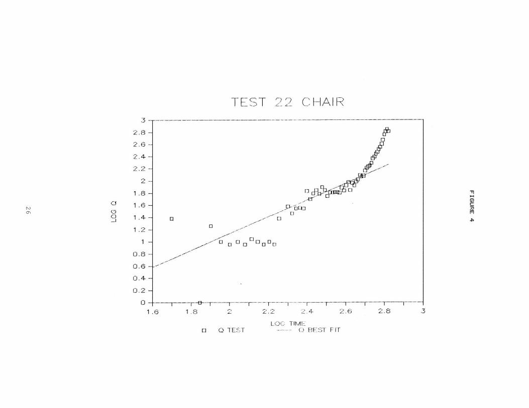
Figure 4 is a log-log plot of data from Test 22 for t = 0 to t
= 660 seconds, which is when the peak heat release rate was reached
during the test. Superimposed on the data is the best fit line which
was calculated using the data from t = 0 to the peak heat release
rate. This regression results in an alpha of 0.0241 kW/sec2 and an
exponent, p, equal to 1.3762.
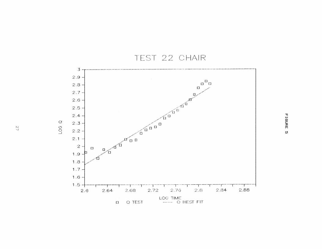
The best fit line does not appear to be a good model for this
data. However, a closer look shows that the data appear to fall
along a straight line from about t = 400 seconds to the peak. Figure
5 shows a best fit line which was found by doing a statistical
regression on the data from 400 to 660 seconds. This line is a much
better model of the data. Alpha was calculated to be 8 x 10-11 and p
was found to be 4.56.
In this case, 400 seconds was arbitrarily selected as the
starting point for the regression analysis. This point will be
referred to as the virtual time of origin, tv, the time when the fire
begins to follow a power-law model. The virtual origin could be
defined as the time at which the fire reaches some minimum heat
release rate or the time at
26
27
28
which radiation from the flame is the dominant means of heat
transfer back to the fuel. Obviously this point will vary from fuel
to fuel and will be dependent on many factors. The rigid definition
of the virtual origin is beyond the scope of this thesis.
The selection of a virtual origin for regression analysis will
depend on which part of the fire you are trying to model. Fitting
the model to only part of the data produces errors. The magnitude
and implications of these errors are discussed later.
For Test 22 the regression analysis from tv = 400 to the peak
at t = 660 seconds produced an exponent equal to 4.56 to be used in
the power-law model. This is more than twice as large as the p = 2
used in Heskestad and Delichatsios' equations. The next step is
determine if a p = 2, power-law model can be fit to the data.
Figure 6 shows heat release rate vs time data for Test 22
plotted on an x-y graph. The best fit power-law curve, based on tv =
400, with alpha = 8 x 10-11 kW/sec2 and p = 4.56 is superimposed. A
curve based on the power-law model, Q = at2, is also plotted. The
value of alpha was varied until the p = 2 model assumed the same
general shape as the test curve. In this case alpha equals 0.0086
kW/sec2. The heat release rate for the p = 2 model was calculated
beginning at t = 0, then plotted beginning at t = tv = 400
29
30
seconds. By varying alpha and tv, the p = 2 model can be
forced to fit the data. Because the heat release rate was
calculated beginning at t = 0, but plotted beginning at t =
400, this curve does not plot as a straight line on a log-log
plot. Regression analyses were not used to determine the
virtual origin or alpha for the p = 2 model. The effects of
errors resulting from the arbitrary selection of alpha and tv
are discussed later.
Figure 6 shows that, initially, the best fit curve is a better
approximation of the actual test data. After about 600 seconds the p
= 2 power-law model is a better approximation of the data.
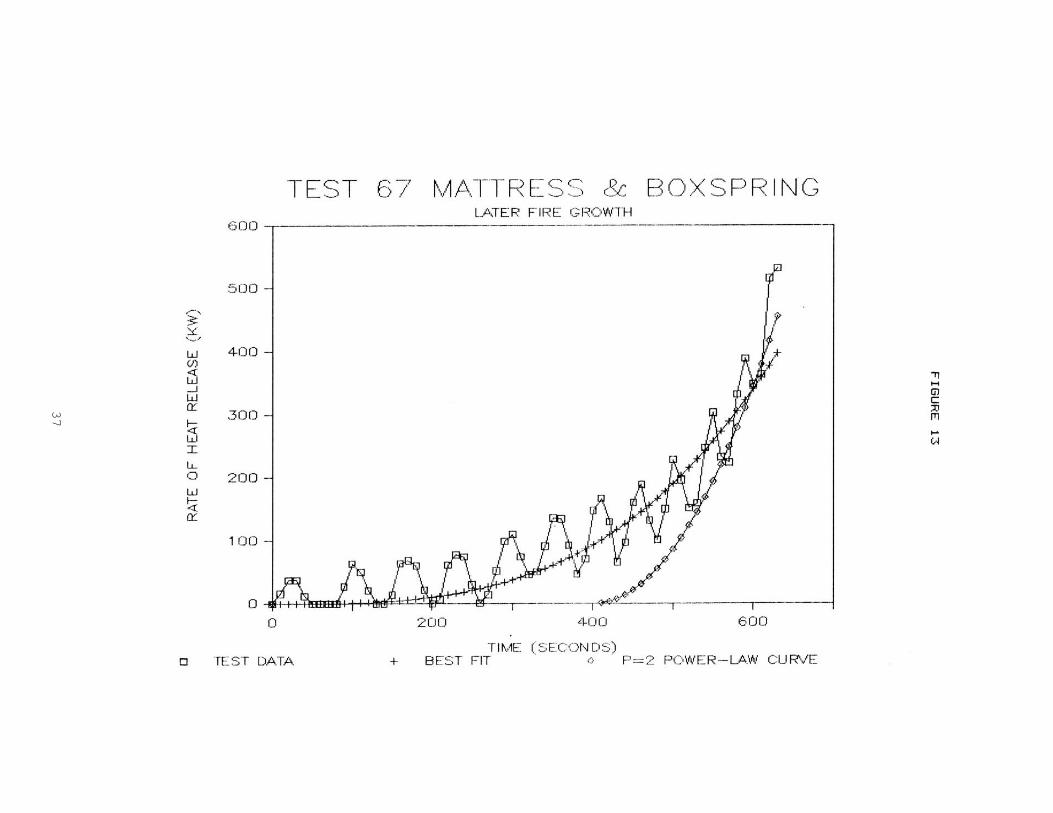
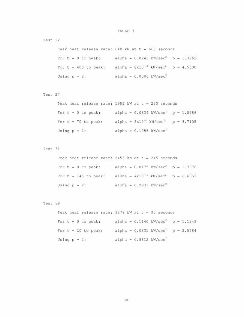
Figures 7 through 13 are plots of several NBS calorimeter
tests along with best fit power-law curves and p = 2 models
superimposed. Table 3 is a summary of the factors (alpha, tv and p)
used to generate the curves. The regression analyses and the
procedures used to establish these curves were the same as those
used in the example for Test 22.
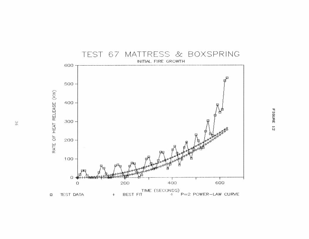
For Test 67, two regression analyses were done, one with tv =
90 seconds and one with tv = 400 seconds. This was done to
demonstrate that different realms of a fire can be modeled with
different curves. The resulting curves are plotted in Figures 12 and
13. The errors resulting from the use of the
31
32
33
34
35
36
37
38
TABLE 3
Test 22
Peak heat release rate: 648 kW at t = 660 seconds
For t = 0 to peak: alpha = 0.0241 kW/sec2 p = 1.3762
For t = 400 to peak: alpha = 8x10-11 kW/sec2 p = 4.5600
Using p = 2: alpha = 0.0086 kW/sec2
Test 27
Peak heat release rate: 1951 kW at t = 220 seconds
For t = 0 to peak: alpha = 0.0334 kW/sec2 p = 1.8586
For t = 70 to peak: alpha = 5x10⁻⁶ kW/sec2 p = 3.7105
Using p = 2: alpha = 0.1055 kW/sec2
Test 31
Peak heat release rate: 2456 kW at t = 245 seconds
For t = 0 to peak: alpha = 0.0175 kW/sec2 p = 1.7076
For t = 145 to peak: alpha = 4x10-13 kW/sec2 p = 6.6652
Using p = 2: alpha = 0.2931 kW/sec2
Test 39
Peak heat release rate: 3278 kW at t = 90 seconds
For t = 0 to peak: alpha = 0.1140 kW/sec2 p = 1.1349
For t = 20 to peak: alpha = 0.0331 kW/sec2 p = 2.5784
Using p = 2: alpha = 0.8612 kW/sec2
39
TABLE 3 CONTINUED
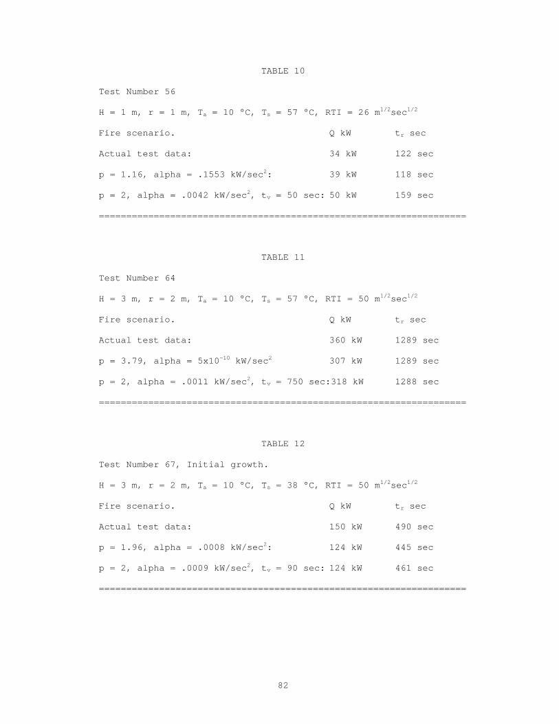
Test 56
Peak heat release rate: 87 kW at t = 170 seconds
For t = 0 to peak: alpha = 2.8669 kW/sec2 p = 0.48316
For t = 50 to peak: alpha = 0.1553 kW/sec2 p = 1.1598
Using p = 2: alpha = 0.0042 kW/sec2
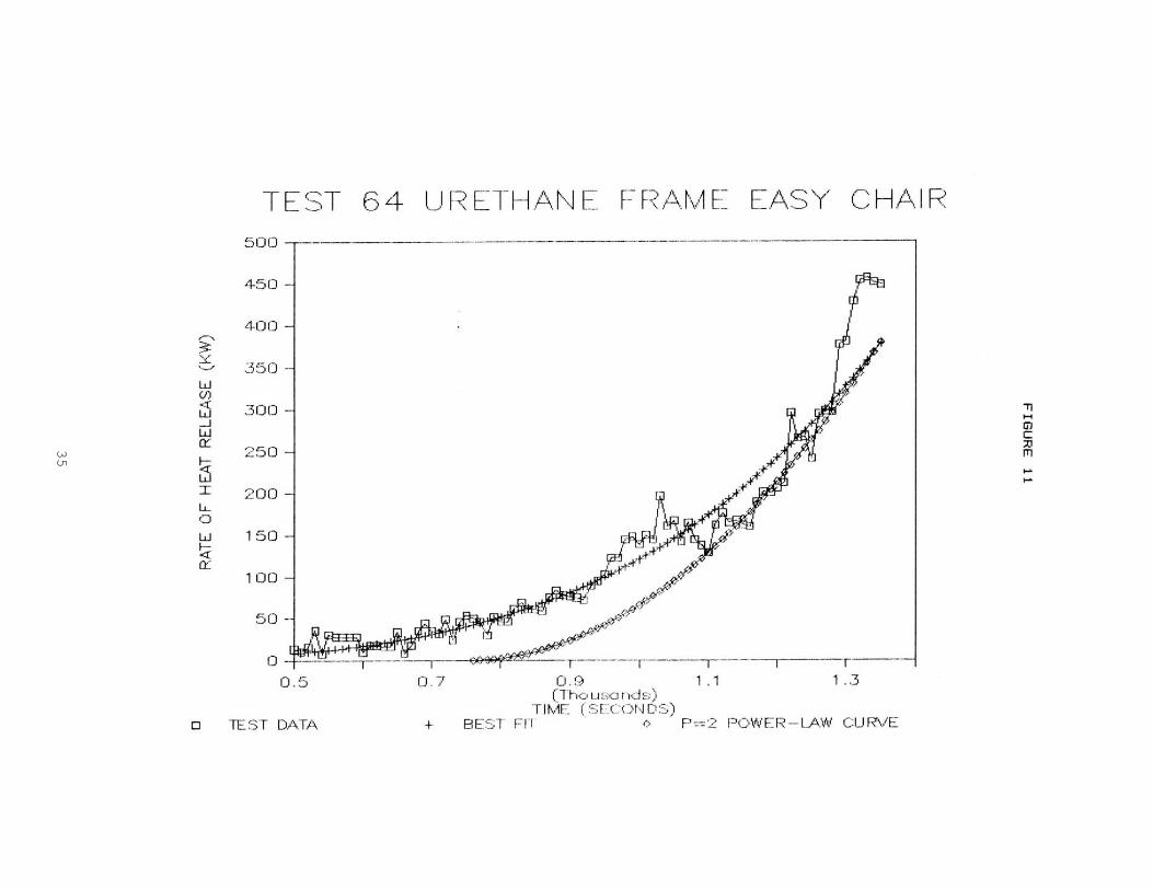
Test 64
Peak heat release rate: 457 kW at t = 1330 seconds
For t = 0 to peak: alpha = 0.0450 kW/sec2 p = 1.0491
For t = 750 to peak: alpha = 5x10⁻¹⁰ kW/sec2 p = 3.7941
Using p = 2: alpha = 0.0011 kW/sec2
Test 67
Peak heat release rate: 532kW at t = 630 seconds
For t = 0 to peak: alpha = 0.1580 kW/sec2 p = 1.0504
For t = 90 to peak: alpha = 0.0008 kW/sec2 p = 1.9630
Using p = 2: alpha = 0.0009 kW/sec2
For t = 400 to peak: alpha = 5x10⁻⁷ kW/sec2 p = 3.1858
Using p = 2: alpha = 0.0086 kW/sec2
40
regression curves or the p = 2 power-law models, as opposed to the
actual test data, are discussed later in terms the effects on the
design and analysis of detector response.
Appendix A contains a set of graphs for forty furniture
calorimeter tests along with p = 2 power-law curves superimposed.
Alpha and tv were not calculated using regression techniques, but
were simply varied until the fits appeared to be good. In many cases
a smaller tv can be used to produce an even better fit to the data.
The use of the larger tv will result in designs of detection systems
which are conservative. The effects of this are discussed later in
terms of the effects on predicted fire size, response time and
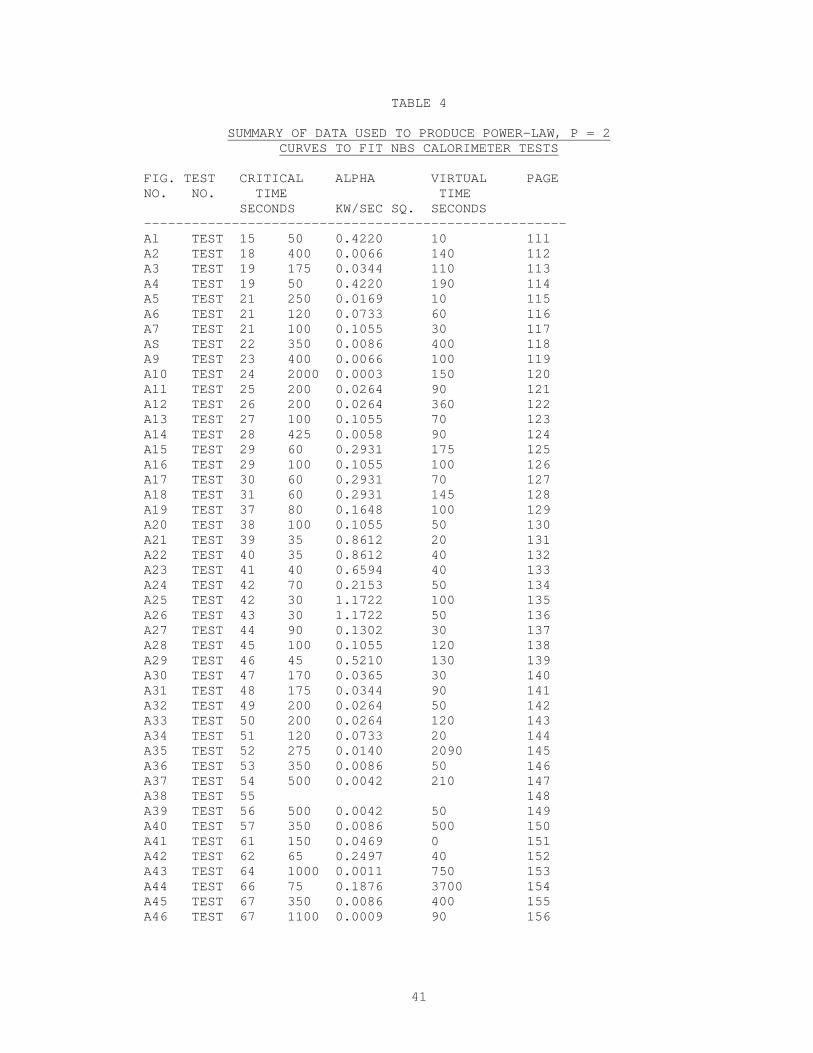
required detector spacing. As with Test 67, for several of the tests
there are more than one graph. Table 4 is summary of the test and
power-law data contained in the appendix.
In all but one test the p = 2, power-law fire growth model
could be used to simulate the initial growth of the fire. Test
Number 55 (Figure 38 of Appendix A), a metal frame chair with a
padded seat never burned at a rate greater than 13 kW. This type of
a fire would fail to activate a fire detector or a sprinkler unless
the detector was very close to the fire. At such low heat outputs,
random convective forces would be as great as the velocities due to
the buoyant flow.
In each of the other test cases it was possible to
41
TABLE 4
SUMMARY OF DATA USED TO PRODUCE POWER-LAW, P = 2 CURVES TO FIT NBS CALORIMETER TESTS
FIG. TEST CRITICAL ALPHA VIRTUAL PAGE NO. NO. TIME TIME SECONDS KW/SEC SQ. SECONDS ----------------------------------------------------- Al TEST 15 50 0.4220 10 1ll A2 TEST 18 400 0.0066 140 112 A3 TEST 19 175 0.0344 110 113 A4 TEST 19 50 0.4220 190 114 A5 TEST 21 250 0.0169 10 115 A6 TEST 21 120 0.0733 60 116 A7 TEST 21 100 0.1055 30 117 AS TEST 22 350 0.0086 400 118 A9 TEST 23 400 0.0066 100 119 A10 TEST 24 2000 0.0003 150 120 All TEST 25 200 0.0264 90 121 A12 TEST 26 200 0.0264 360 122 A13 TEST 27 100 0.1055 70 123 A14 TEST 28 425 0.0058 90 124 A15 TEST 29 60 0.2931 175 125 A16 TEST 29 100 0.1055 100 126 A17 TEST 30 60 0.2931 70 127 A18 TEST 31 60 0.2931 145 128 A19 TEST 37 80 0.1648 100 129 A20 TEST 38 100 0.1055 50 130 A21 TEST 39 35 0.8612 20 131 A22 TEST 40 35 0.8612 40 132 A23 TEST 41 40 0.6594 40 133 A24 TEST 42 70 0.2153 50 134 A25 TEST 42 30 1.1722 100 135 A26 TEST 43 30 1.1722 50 136 A27 TEST 44 90 0.1302 30 137 A28 TEST 45 100 0.1055 120 138 A29 TEST 46 45 0.5210 130 139 A30 TEST 47 170 0.0365 30 140 A31 TEST 48 175 0.0344 90 141 A32 TEST 49 200 0.0264 50 142 A33 TEST 50 200 0.0264 120 143 A34 TEST 51 120 0.0733 20 144 A35 TEST 52 275 0.0140 2090 145 A36 TEST 53 350 0.0086 50 146 A37 TEST 54 500 0.0042 210 147 A38 TEST 55 148 A39 TEST 56 500 0.0042 50 149 A40 TEST 57 350 0.0086 500 150 A41 TEST 61 150 0.0469 0 151 A42 TEST 62 65 0.2497 40 152 A43 TEST 64 1000 0.0011 750 153 A44 TEST 66 75 0.1876 3700 154 A45 TEST 67 350 0.0086 400 155 A46 TEST 67 1100 0.0009 90 156
42
obtain a p = 2, power-law curve to model the fire growth. In five
cases the test specimens exhibited different realms of burning. Each
of the realms is modeled by different power-law fire growth curves
as was shown above for Test 67. These tests are numbers 19, 21, 29,
42 and 67.
Figures 14 and 15 are of NBS Test Number 19. This chair had a
wood frame and was covered with a polyurethane foam padding. The
fabric covering this typical easy chair was a polyolefin fabric. The
first graph shows the initial stage of the fire growth in Test 19.
The second graph shows the complete development of the fire.
If interested in the initial growth of this type of fire, it
can be modeled with the curve shown in Figure 14. This graph shows
that the heat release rate of the fire increases rapidly at about
140 seconds after ignition. At about 200 seconds the chair is
burning at a rate of 300 kW (284 BTU/sec). To model the fire growth,
use:
Qp (kW) = a(kW/sec2)(t - tv)
2(sec2) [20]
or:
Qp (kW) = [1055 (kW)/tc2(sec)] (t - tv)
2(sec) [21]
With:
a = 0.0344 kW/sec2 or tc = 175 sec
tv = 110 sec
43
44
45
To make the p = 2, power-law curve fit, it must have a virtual
origin of 110 seconds. This causes the curve to fit the actual data
after about 140 to 150 seconds. Between 110 and 140 seconds, the
temperature and velocity of the gases predicted by the equations
developed by Heskestad and Delichatsios would be slightly in error.
The error would be on the conservative side when the equations are
used to design a detection system. This is because the predicted
heat release rate is slightly below the actual measured value at a
given time. The model will then predict lower temperatures and
velocities in the fire plume and across the ceiling. This causes a
fire detector or sprinkler, located a distance r and a height H from
the fire, to respond sooner to the real fire than to the model.
If a latter stage in the development of the fire is of
interest, Figure 15 shows a model curve which could be used. This
burning realm of Test 19 is modeled by a p = 2 power-law growth with
alpha = 0.422 (kW/sec2) and a virtual origin of 190 seconds.
The graphs of the forty tests show that the power-law fire
growth model, Q = atp, with p = 2 can be used to model different
stages of the initial development of the furniture calorimeter
fires. The main difficulty arises when trying to select the proper
value for the fire growth parameter, alpha. As more data becomes
available from furniture calorimeter
46
tests and other fire tests, fire protection engineers will be better
able to make estimates of alpha for furnishings and commodities in
an area they might be studying.
Appendix A is a catalog of fire growth parameters for
different fuels. Engineers can use it to select the approximate fire
growth characteristics necessary to model similar fuel packages
using Heskestad and Delichatsios' equations or the graphs and tables
of NFPA 72-E, Appendix C. The data contained in Appendix A is best
used in conjunction with the original NBS reports on the calorimeter
tests (References 12 and 16). In addition to heat release rate, the
NBS reports contain data such as rate of mass loss, particulate
conversion and target irradiance, plotted as a function of time.
Appendix A shows that a p = 2, power-law model can be used to
model open air furniture fires. As shown above, a regression
analysis can be done to determine the exponent and the alpha which
best fit the test data. However, the objective here is to show how
engineers can use the p = 2 power-law equations proposed by
Heskestad and Delichatsios to design and analyze detector response.
The effects of using p = 2 are discussed later.
47
5. RESPONSE MODEL FOR HEAT DETECTORS
AND AUTOMATIC SPRINKLERS
The power-law fire growth model combined with the
similarity equations proposed by Heskestad and Delichatsios,
defines the environment of a sprinkler or fire detector in terms
of the temperature and velocity of fire gases across the ceiling.
The relationship found in the Factory Mutual test data between
optical density and the change in temperature at a point, can be
used to estimate the optical density as a function of time during
the initial growth of the fire. The next step is to combine these
relationships with models which define the response of
commercially available sprinklers and fire detectors.
Table 5 is a cross reference of fire signatures and
commercially available detector types. The table shows which
units respond to the various fire signatures listed. It should be
noted that the detector types which respond to heat are also
affected by infrared or thermal radiation. However in the initial
stages of fire growth, convective heating by the fire gases will
be the predominant means of heat transfer. In addition, because
most sprinklers and fire detectors have a relatively small
surface area and respond at temperatures below 300 degrees
Fahrenheit, the radiation to and from the units can ignored when
calculating their response.
48
49
The response of ultraviolet and infrared fire detectors can
not be modeled directly using Heskestad and Delichatsios's fire
model. The response of these detector types is beyond the scope
of this paper.
Figure 16 describes the heat transfer taking place between
a heat detector or sprinkler and its environment. The total heat
transfer rate to the unit, qtotal, can be described by:
Norwood, MA 02062. 4. "Recommended Practices", Industrial Risk Insurers,
Hartford, CT 06102. 5. I. Benjamin, G. Heskestad, R. Bright and T. Hayes, "An
Analysis of the Report on Environments of Fire Detectors", Fire Detection Institute, 1979.
6. G. Heskestad and M. Delichatsios, "Environments of Fire
Detectors - Phase I: Effect of Fire Size, Ceiling Height and Material." Volume I "Measurements" (NBS-GCR-77-86), May 1977, Volume II “Analysis" (NBS-GCR-77-95), June 1977, National Technical Information Service (NTIS) Springfield, VA 22151.
7. C. Beyler, "A Design Method For Flaming Fire Detection",
Fire Technology, Volume 20, Number 4, November, 1984. 8. G. Heskestad, "Similarity Relations for The Initial
Convective Flow Generated by Fire", ASME Paper No. 72-WA/HY-17, 1972.
9. G. Heskestad, "Physical Modeling of Fire", Journal of Fire
and Flammability, Volume 6, July 1975. 10. G. Heskestad, "Engineering Relations for Fire Plumes",
Technology Report 82-8 Society of Fire Protection Engineers, 60 Batterymarch St., Boston, MA 02110, 1982.
11. J.D. Seader and W.P. Chien, "Physical Aspects of Smoke
Development in an NBS Smoke Density Chamber," Journal of Fire and Flammability, Volume 6, July 1975.
12. V. Babrauskas, J.R. Lawson, W.D. Walton and W.H. Twilley,
"Upholstered Furniture Heat Release Rates Measured with a Furniture Calorimeter", U.S. Department of Commerce, National Bureau of Standards, National Engineering Laboratory, Center for Applied Mathematics, Center for Research, Washington, D.C. Number NBSIR 822604, December 1982.
107
13. C. Huggett, "Estimation of Rate of Heat Release By Means of Oxygen Consumption Measurements", Fire and Materials. 4, 61-5, 1980.
14. W.J. Parker, "Calculation of the Heat Release Rate by
Oxygen Consumption for Various Applications", U.S. Department of Commerce, National Bureau of Standards, National Engineering Laboratory, Center for Applied Mathematics, Center for Research, Washington, D.C. Number NBSIR 81-2427, 1982.
15. D. Drysdale, "An Introduction to Fire Dynamics", John Wiley
and Sons, N.Y., N.Y., 1985. 16. J.R. Lawson, W.D. Walton and W.H. Twilley, "Fire
Performance of Furnishings as Measured in the NBS Furniture Calorimeter, Part I", U.S. Department of Commerce, National Bureau of Standards, National Engineering Laboratory, Center for Applied Mathematics, Center for Research, Washington, D.C. Number NBSIR 83-2787, August 1993.
17. G. Heskestad and H. Smith, "Investigation of a New
Sprinkler Sensitivity Approval Test: The Plunge Test," FMRC Serial Number 22485, Factory Mutual Research Corp., 1976.
18. J.P. Hollman, "Heat Transfer," McGraw-Hill Book Company, N.
Y. , N. Y. , 1976. 19. W. Bissell, private communication. 20. G. Heskestad and M. Delichatsios, "The Initial Convective
Flow in Fire," Seventeenth Symposium (International) on Combustion, The Combustion Institute, 1979.
21. C. Beyler, private communication. 22. R. Alpert, "Calculation of Response Time of Ceiling Mounted
Fire Detectors," Fire Technology, Volume 8, 1972. 23. D. Evans and D. Stroup, "Methods to Calculate the Response
Time of Heat and Smoke Detectors Installed Below Large Unobstructed Ceilings," U.S. Department of Commerce, National Bureau of Standards, National Engineering Laboratory, Gathersburg, MD. Number NBSIR 85-3167, February 1985, issued July 1985.