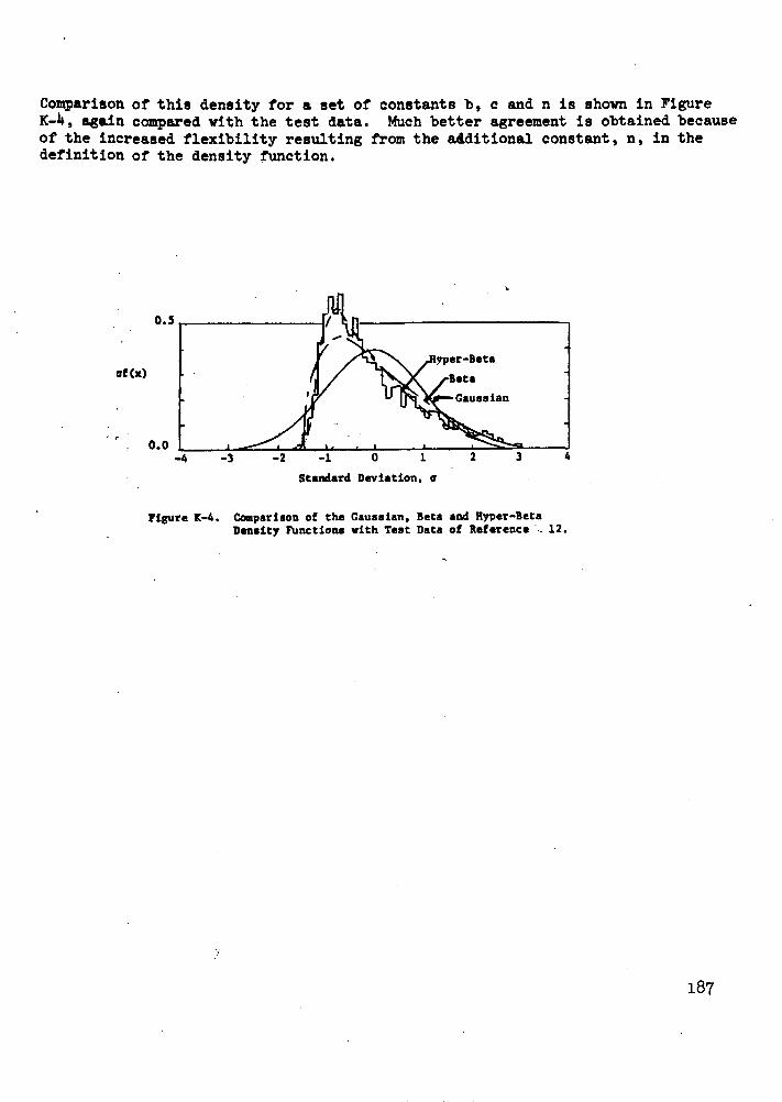
NASA CR 114577 (Available to the Public) ANALYSIS OF INLET FLOW DISTORTION AND TURBULENCE EFFECTS ON COMPRESSOR STABILITY By H. C. MELICK 31 March 1973 Distribution of this report is provided in the interest of information exchange. Responsibility for the contents resides in the: author or organization that prepared it. iCOB PR SOR STABILITY (LTV Aerospace Corp.) CSCL 21E Unclas Prepared- Hn na e Uv. G3/28 68331 By VOUGHT SYSTEMS DIVISION LTV AEROSPACE CORPORATION'. ,e, ·. ,?_~ "., National Ae For ;,"'N ' eronautics and Sp .Ad is-tration Ames Research Center Moffett Field, California rv, JhP , .. / V, AUKS Sn'tS , https://ntrs.nasa.gov/search.jsp?R=19730012966 2019-04-08T21:09:01+00:00Z
Transcript
NASA CR 114577(Available to the Public)
ANALYSIS OF INLET FLOWDISTORTION AND TURBULENCE EFFECTS
ON COMPRESSOR STABILITY
By
H. C. MELICK
31 March 1973
Distribution of this report is provided in the interest ofinformation exchange. Responsibility for the contentsresides in the: author or organization that prepared it.
iCOB PR SOR STABILITY (LTV Aerospace Corp.)
CSCL 21EUnclasPrepared- Hn na e Uv. G3/28 68331
By
VOUGHT SYSTEMS DIVISIONLTV AEROSPACE CORPORATION'.
,e, ·. ,?_~ ".,
National Ae
For ;,"'N '
eronautics and Sp .Ad is-trationAmes Research Center
The effect of steady state circumferential total pressure distortion onthe loss in compressor stall pressure ratio has been established by analyticaltechniques. Full scale engine and compressor/fan component test data wereused to provide direct evaluation of the analysis. Favorable results of thecomparison are considered verification of the fundamental hypothesis of thisstudy. Specifically, since a circumferential total pressure distortion inan inlet system will result in unsteady flow in the coordinate system of therotor blades, an analysis of this type distortion must be performed from anunsteady aerodynamic point of view. By application of the fundamentalaerothermodynamic laws to the inlet/compressor system, parameters importantin the design of such a system for compatible operation have been identified.A time constant, directly related to the compressor rotor chord, was found tobe significant, indicating compressor sensitivity to circumferential dis-tortion'is directly dependent on the rotor chord.
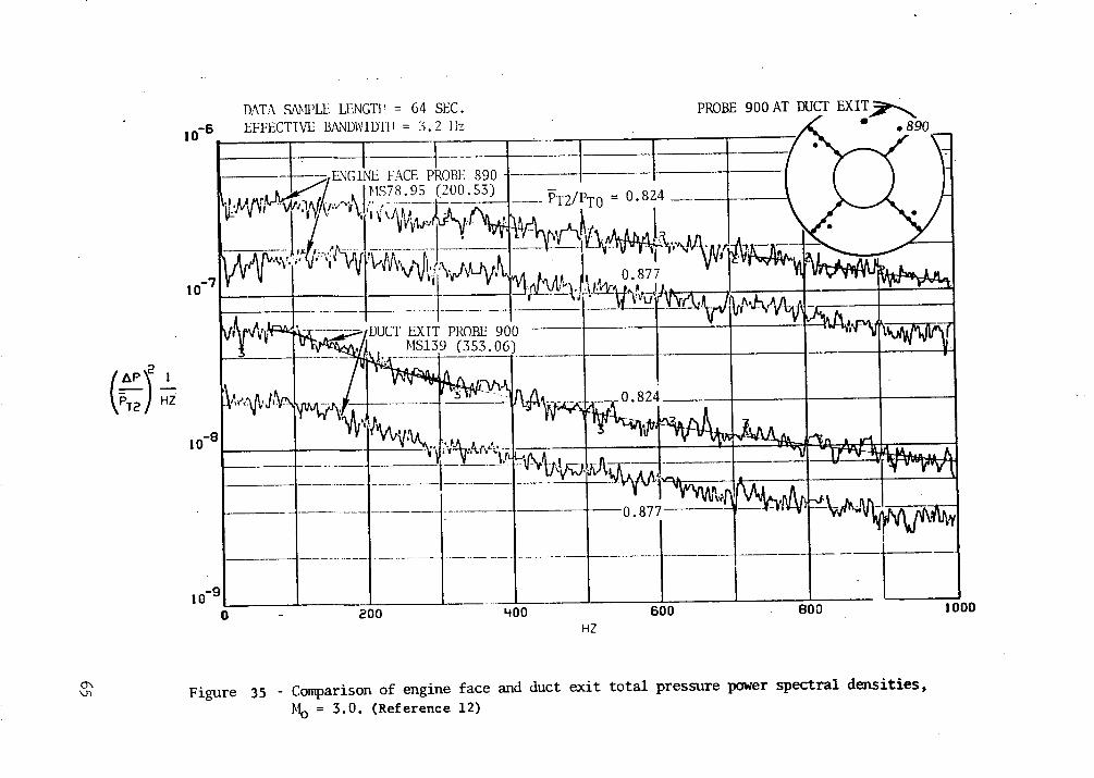
As an initial step in the investigation of the effects of time dependenttotal pressure distortion on the compressor stability characteristics, ananalytical model of turbulent flow typical of that found in aircraft inletshas also been developed. Due to the non-deterministic (random) nature ofthis type of flow distortion, the flow analysis requires use of statisticalmethods. These methods were combined with basic fluid dynamic conceptsto provide a usable analysis technique. With this model, the power spectraldensity function and root mean square level of the time dependent totalpressure take on considerable significance as indicators of the strength andextent of low pressure regions that are important in the compressor reactionto inlet flow disturbances. Spectra obtained from the model were comparedwith those obtained in tests of a Mach 3 mixed compression inlet to illustratethe technique of determining the mean size and strength of instantaneous lowpressure regions by statistical techniques and to verify the turbulent flowmodel. Excellent agreement was obtained in the comparison verifying thisfundamental approach.
Both the steady state distortion/compressor analysis and the turbulentflow model are considered developed to the point necessary to initiate thedevelopment program to achieve the long term program objective of combiningthese results to establish a fundamental relationship between both inletsteady state circumferential distortion and turbulence and loss in compressorstall margin.
1
Preceding page blankINTRODUCTION
Inlet/engine system stability problems have grown to major proportionswith the continuing press to improve performance and reduce system weight andvolume. The need to solve such problems and to understand the effect ofinlet total pressure distortion on engine compressor stability has becomecritical. To date, solutions to the problem of inlet/engine compatibilityhave had to come from experimental results since adequate stability analysismethods were not available. This has resulted in extensive inlet and enginetest requirements. Notwithstanding, the important design variables forinlet/engine stability remained obscure.
An analytical approach that considers the fundamentals of the dynamicinteraction between inlet flow and engine compressor is needed to augment theuse of the traditional empirical distortion factors. The method needs tobe sufficiently detailed to provide insight into the basic interaction andyield workable accuracy, yet not detailed to the point of being expensiveand cumbersome to apply.
This program,initiated in April 1972, has been oriented towarddeveloping basic relationships between inlet flow distortion and turbulenceand the loss in compressor stall margin. A five task approach has beenestablished. The initial two phases, which comprise the subject matter ofthis report, were designed to develop the fundamental techniques requiredfor successful completion of the program. Future studies combine thesefundamental analyses to relate inlet flow distortion and turbulence to theloss in compressor stall margin. These analyses can then be used withdata from existing inlet/engine tests to establish procedures capable ofpredicting compressor stability margin during the design phase of apropulsion system.
The objective of Task I is to develop an analytical technique to relateinlet circumferential total pressure distortion to the loss in compressorstall margin. A steady state circumferential distortion appears as timevariant in the rotor coordinate system. The developed analysis is uniquesince it considers the effects of this unsteady flow on the compressor stagecharacteristics. Secondly, the effects of flow distortion are established byconsideration of only the stall margin changes caused by distortion,eliminating need for detailed construction of individual stage and compressorperformance maps. Favorable comparison between results of the analysis andexperimental data are considered to have verified this approach.
The objective of Task II is to develop a statistical model of inletturbulent flow. This was accomplished by the combination of two engineer-ing disciplines: fluid mechanics and statistical mathematics. Based onthe fundamental hypothesis that the time dependent total pressure fluctua-tions are a direct result of streamline curvature rather than acoustic waves,it was assumed that these pressure fluctuations could be described by arandom distribution of descrete vortices transported by the mean flow. Thelaws of fluid mechanics were used to describe the fluid dynamic character-istics of the vortices, while the statistical methods were used to handlethe random properties of the flow. Results of the analysis were verified bytest data. Through this model easily measured inlet flow properties such astotal pressure RMS level and power spectral density function can be inter-preted in a context meaningful to engine stability.
PRECEDING PAGE BLANK NOT FILMED
Preceding page blank
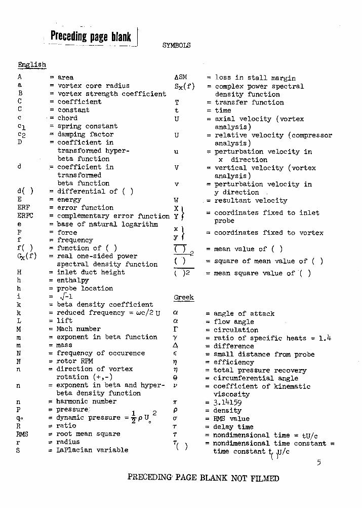
= area= vortex core radius= vortex strength coefficient= coefficient= constant= chord= spring constant= damping factor= coefficient intransformed hyper-beta function
= coefficient intransformedbeta function
= differential of ( )= energy= error function= complementary error function= base of natural logarithm= force= frequency= function of ( )= real one-sided powerspectral density function
= inlet duct height= enthalpy= probe location
= beta density coefficient= reduced frequency = wc/2 U= lift= Mach number= exponent in beta function- mass
= frequency of occurence= rotor RPM= direction of vortexrotation (+,-)
= exponent in beta and hyper-beta density function
TASK IEFFECT OF STEADY STATE TOTAL PRESSURE DISTORTION ON COMPRESSOR STALL MARGIN
The objective of Task I is to relate inlet circumferential steady statetotal pressure distortion to loss in engine compressor stall margin. An ana-lytical technique based on the fundamental aero-thermodynamic laws governingfluid flow and engine compressor operation has been developed. The generalapproach is outlined below and the details presented in subsequent sections.
Distorted inlet flow is composed of total pressure levels both above andbelow the average. These regions correspond to deviations in axial flowvelocity from the mean. In the rotating coordinate system of the rotor, thesedeviations appear as fluctuations in the stream angle or angle of attack rela-tive to the rotor blades. Therefore, the flow over the rotor blades isbasically unsteady and hence steady state distortion, as well as unsteady, mustbe analyzed by unsteady aerodynamic techniques. Accordingly, as a basis forthe study, the effects of a time varying angle of attack on the liftingcharacteristics of an isolated airfoil are established. The results are thenapplied to a compressor rotor blade and by relating the work done by therotor to the lifting characteristics of the blades, the loss in compressorstall margin due to an arbitrary circumferential distortion pattern isestablished.
Isolated Airfoil Analysis
The primary objective of this specific item is to establish the effectof unsteady airflow on the lifting characteristics, and in particular on themaximum lift coefficient, of an isolated airfoil. This will include resolu-tion of the effects for arbitrary transients in angle of attack. To accomplishthis objective, it is first necessary to understand the flow phenomenainvolved in delaying the stall of an airfoil beyond its steady state charac-teristics when the airfoil is subjected to an unsteady angle of attackand then develop a mathematical representation of the process which can besolved for arbitrary, time dependent, angles of attack.
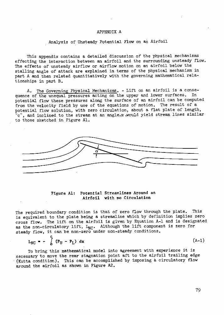
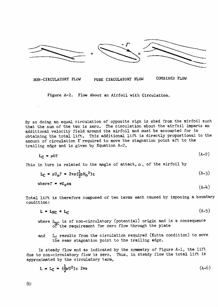
Effect of Unsteady Flow on Lift. - Lift on an airfoil is a consequenceof unequal pressures acting on the upper and lower surfaces. In potentialflow these pressures can be computed from the velocity field by use of theequations of motion. In the case of unsteady flow, the lift is dependentnot only on the instantaneous angle of attack but also on the following twofactors: (1) the inertia or acceleration of the mass of air in proximityof the airfoil and, (2) the shedding of the trailing edge vortex which actsas a dissipative force. The phenomena are analogous to the forces andacceleration of a damped mass/spring system which can be described by alinear second order differential equation. Similarly, the lift of an air-foil subjected to an unsteady flow can be described in the same manner.As an example, the lift per unit span due to an airfoil undergoing verticaloscillations at an angular frequency of is:
L(t) ' 1 · + [UwpcC(k) dy + U2c (1)L Jdt+ dt L (
2rPCwhere: TfP- = virtual mass
7rpcC(k) = "dissipation constant"
C(k) = function of reduced frequency, k
k = £dc/2U
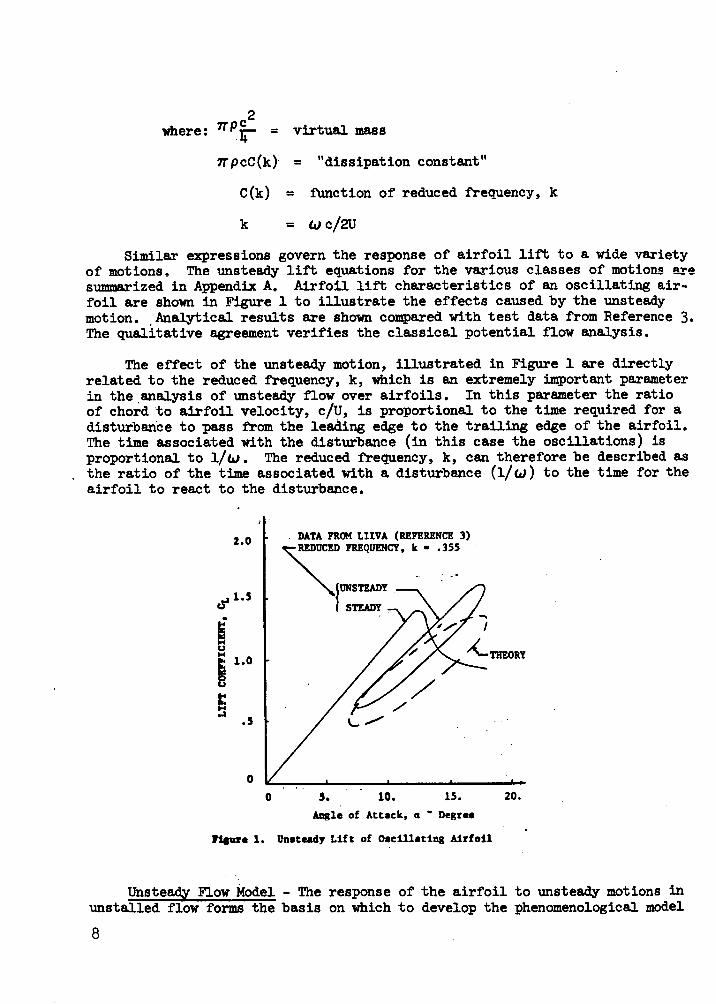
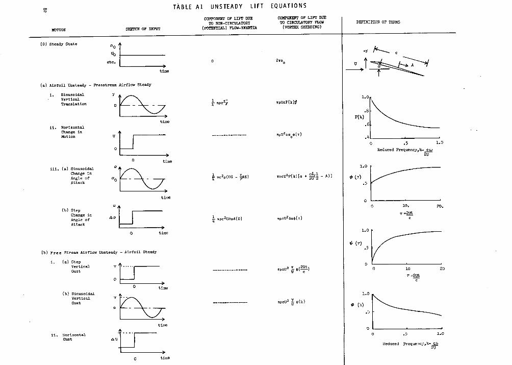
Similar expressions govern the response of airfoil lift to a wide varietyof motions. The unsteady lift equations for the various classes of motions aresummarized in Appendix A. Airfoil lift characteristics of an oscillating air-foil are shown in Figure 1 to illustrate the effects caused by the unsteadymotion. Analytical results are shown compared with test data from Reference 3.The qualitative agreement verifies the classical potential flow analysis.
The effect of the unsteady motion, illustrated in Figure 1 are directlyrelated to the reduced frequency, k, which is an extremely important parameterin the analysis of unsteady flow over airfoils. In this parameter the ratioof chord to airfoil velocity, c/U, is proportional to the time required for adisturbance to pass from the leading edge to the trailing edge of the airfoil.The time associated with the disturbance (in this case the oscillations) isproportional to 1/W. The reduced frequency, k, can therefore be described asthe ratio of the time associated with a disturbance (1/LC) to the time for theairfoil to react to the disturbance.
2.0
1.5
IE1.
. 5
0
DATA FROM LIIVA (REFERENCE 3)-REDUCED FREQUENCY, k - .355
0 5. 10. 15. 20.Angle of Attack, a ' Degree
OFlre 1. Unsteady Lift of Oscillating Airfoil
Unsteady Flow Model - The response of the airfoil to unsteady motions inunstalled flow forms the basis on which to develop the phenomenological model
8
of an isolated airfoil subjected to angle of attack excursions beyond the steadystate stall limit. This is achieved by modeling the physical mechanismsinvolved with a stalling airfoil via the concept of an effective angle of attack.
When a airfoil is subjected to unsteady variations in angle of attack, thepressure distribution about the airfoil does not correspond to that associatedwith the steady state condition for the instantaneous value of angle of attack.This is due to the finite amount of time required for flow about an airfoilto adjust to the variations in angle of attack. Flow phenomena requiringadjustment include the external flow, shed vorticity, and the boundary layer.Initially the flow at the airfoil leading edge experiences the change in angleof incidence. At later times this new flow angle is felt at subsequent stationsalong the chord of the airfoil. Therefore an effective angle of attack, a eff,is hypothesized which lags the instantaneous angle. This angle accounts for thefinite time required for airflow adjustment and boundary layer separation tooccur and is modeled mathematically below to enable prediction of the stallinglift coefficient of an airfoil operating in unsteady flow.
In keeping with the findings of an unstalled airfoil, it is assumed thatthe physical mechanisms are governed by a linear second order differentialequation.. Thus, the relationship between the effective and instantaneous angleof attack can be written as:
Cinst = actual (instantaneous) angle of attack at time, t
aeff = effective angle of attack
a0 = angle of attack about which the perturbations occur.o
The time constants, Tl and r2 are associated with the airfoil/airflow system
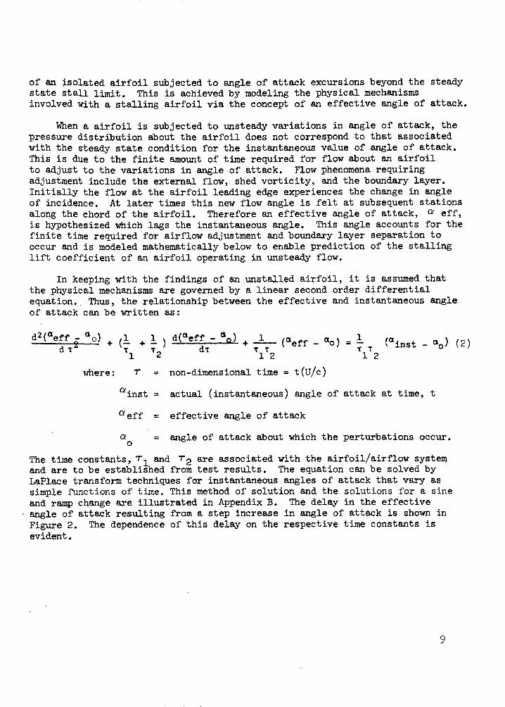
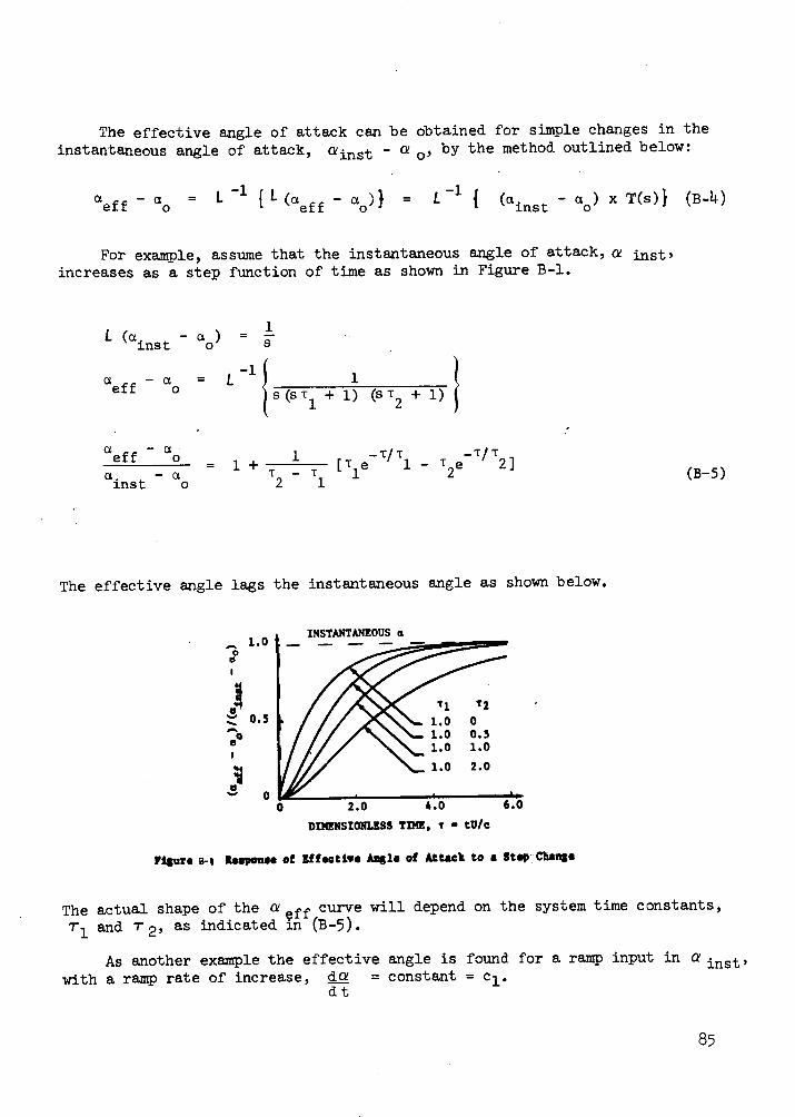
and are to be established from test results. The equation can be solved byLaPlace transform techniques for instantaneous angles of attack that vary assimple functions of time. This method of solution and the solutions for a sineand ramp change are illustrated in Appendix B. The delay in the effectiveangle of attack resulting from a step increase in angle of attack is shown inFigure 2. The dependence of this delay on the respective time constants isevident.
9
1.0
lO
0.5
a0.5.5
00 2.0 4.0 6.0
DIMZlmSIONLSS TDm, T - tU/c
Flgure 2. Response of Effective An1le of Attack to a Step- Change
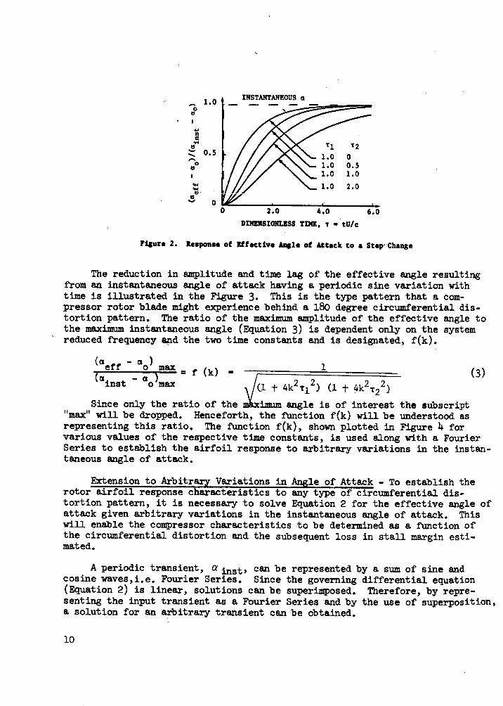
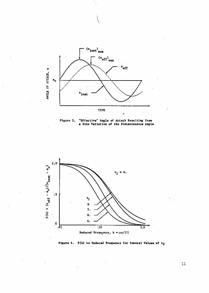
The reduction in amplitude and time lag of the effective angle resultingfrom an instantaneous angle of attack having a periodic sine variation withtime is illustrated in the Figure 3. This is the type pattern that a com-pressor rotor blade might experience behind a 180 degree circumferential dis-tortion pattern. The ratio of the maximum amplitude of the effective angle tothe maximum instantaneous angle (Equation 3) is dependent only on the systemreduced frequency and the two time constants and is designated, f(k).
(aeff a) max(a a-n f (k) = (3)inst o max (1 + 4k2 12) (1 t 4k2 T2 2)
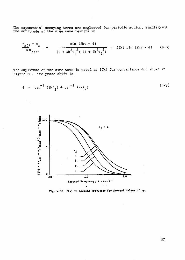
Since only the ratio of the nbimum angle is of interest the subscript"max" will be dropped. Henceforth, the function f(k) will be understood asrepresenting this ratio. The function f(k), shown plotted in Figure 4 forvarious values of the respective time constants, is used along with a FourierSeries to establish the airfoil response to arbitrary variations in the instan-taneous angle of attack.
Extension to Arbitrary Variations in Angle of Attack - To establish therotor airfoil response characteristics to any type of circumferential dis-tortion pattern, it is necessary to solve Equation 2 for the effective angle ofattack given arbitrary variations in the instantaneous angle of attack. Thiswill enable the compressor characteristics to be determined as a function ofthe circumferential distortion and the subsequent loss in stall margin esti-mated.
A periodic transient, a inst, can be represented by a sum of sine andcosine waves,i.e. Fourier Series. Since the governing differential equation(Equation 2) is linear, solutions can be superimposed. Therefore, by repre-senting the input transient as a Fourier Series and by the use of superposition,a solution for an arbitrary transient can be obtained.
10
I
TIME
Figure 3. "Effective" Angle of Attack Resulting froma Sine Variation of the Instantaneous Angle
m 4.
'2
0
1.
4.
8.
.01 .10 1.0
Reduced Frequency, k wc/2U
Figure 4. f(k) vs Reduced Frequency for Several Values of T2
11
o
0
1.00
V
1 .5
-4
0
The Fourier Series representation is as follows:
00 oo
ainst (e) = a + CEn cos (ne) + b sin (ne) (4)n=1 n=l
Where: n = the harmonic number
0a = average angle of attack
an, bn = Fourier Coefficients
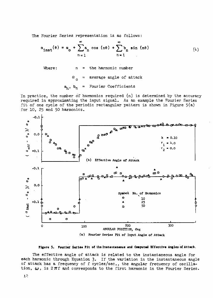
In practice, the number of harmonics required (n) is determined by the accuracyrequired in approximating the input signal. As an example the Fourier Seriesfit of one cycle of the periodic rectangular pattern is shown in Figure 5(a)for 10, 25 and 50 harmonics.
-0.1o
Ctb cP° MY c10 au OA
o 0.0 r0 0 ,aOO0. A I k -0.10
' OP · -4.o
· op
2
-- O .O
+0.1 (b) Effective Angle of Attack
0.0
0 Symbol No. of Harmonics
, 0 10+0.1 A 25
'f o o 50
0 0
o 100 200 300ANGULAR POSITION, deg
(a) Fburier Series Fit of Input Angle of Attack
Figure 5. Fourier Series Fit of the Instantaneous and Computed Effective Angles of Attack.
The effective angle of attack is related to the instantaneous angle foreach harmonic through Equation 3. If the variation in the instantaneous angleof attack has a frequency of f cycles/sec., the angular frequency of oscilla-tion, Ad, is 27rf and corresponds to the first harmonic in the Fourier Series.
12
The second harmonic will be twice 27rf or 47rf. In general, the angularfrequency of the nth harmonic will be n(27rf). Equation 3 can now be appliedto each harmonic as illustrated in Equation 5.
In general:
aine f - = f(n k )
(5)
The effective angle of attack of the total input signal is found by adding thesolutions for the individual harmonic as indicated by Equation 6.
(eff) - = Z f(nk) a ncos (nO + Y(nk) + Z f(nk) b sin (nO + Y(nk)n=l nn=l
where i(nk) = tan -1
(2nkTl) + tan- 1
(2nk¶2) (6)
The results for the rectangular periodic pattern are shown in Figure 5(b) foran increasing number of harmonics. Although an accurate fit of the rectangularwave requires a large number of harmonics, the effective angle is relativelyinsensitive to this number.
Airfoil Dynamic Stall - Stall of an airfoil in unsteady flow occurs athigher instantaneous angles of attack than that obtained under steady stateflow conditions. This is indicated schematically in Figure 6(a), where thepoint "D" represents the instantaneous stall point and "B" the steady statestall point. This concept results in a time lag in the airfoil response to theunsteady airflow and a reduction in the maximum effective angle of attack.Both of these items are due to the finite time required for the airflow aboutthe airfoil to adjust. This lag in response is indicated in Figure 6(b) fora sinusoidal variation in angle of attack and superimposed on the airfoilcharacteristic in Figure 6(c). The relationship governing this effective angleof attack is given by Equation 6. It is hypothesized that when aeff is equalto the steady state stall value, stall during unsteady flow will occur. Thus,in Figure 6(b) when ca ff reaches the steady state stall line (line B) theairfoil will stall. This stall condition, a eff = C sssis represented for asinusoidal oscillation by Equation 7.
- f(k) (7)ainst -o
Solution of Equation 7 for the instantaneous angle of attack will yield themaximum allowable value for the specific, f(k). Thus:
eaff C0O - steady state (or mean operating point)B - steady state stallC - maximum instantaneous excursionD - "instantaneous" stall point
/ 9/ E - maximum effective angle
a
(c) Effect of Sinusoidal Oscillationson Airfoil Lift
Figure 6. The Effect of Sinusoidal Oscillation on Airfoil Characteristics
The increase in maximum (stalling) angle of attack of an airfoil will there-fore be:
ma inmax a sss (asss -)[ 1] (9max inst max sss SSS o 0 f(7 ~(9)
This will be the increase in the stalling value of a i as indicated bypoint D in Figure 6(a). The function f(k) is dependent on the respectivesystem time constants, T 1 and r2, and the reduced frequency, k.
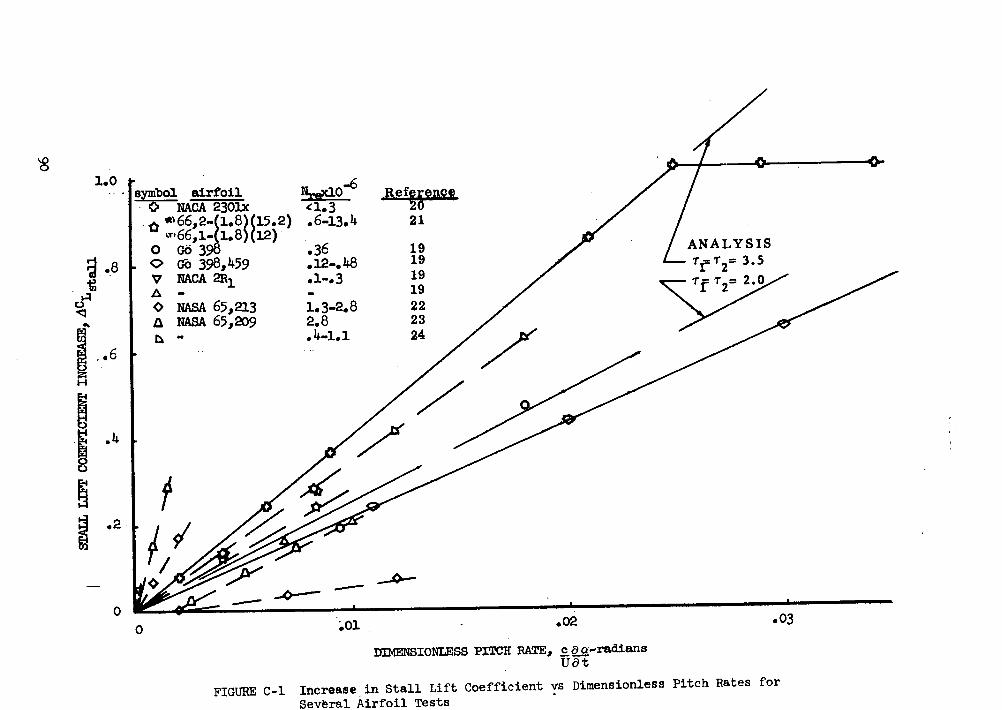
To establish an estimate of the time constants a limited literature survey
of the effect of unsteady flow on the maximum lift coefficient of an airfoilwas conducted and is presented in Appendix C. Results indicate that the timeconstants are approximately equal and on the order of 3.5c/U.
In summary, it was found that the response of a lifting airfoil to anunsteady change in angle of attack was in general governed by a second orderlinear differential equation. To represent this unsteady process which is afunction of the time required for airflow accelerations, shedding of necessarytrailing edge vortices, and the delay of boundary layer separation, aneffective angle of attack was hypothesized. By means of this effective angleof attack a mathematical representation of the increase in stalling lift co-efficient is established by solution of the governing differential equation.This is considered an important development since it enables the responsecharacteristics of a rotor airfoil subjected to unsteady flow conditions tobe determined. These characteristics can then be incorporated into a com-pressor analysis.
Compressor Analysis
The response of a compressor rotor to circumferential total pressuredistortion will be established by first relating the change in rotor airfoilangle of attack caused by the distortion to the required change in compressorpressure ratio. This result will then be combined with the unsteady flow modelfor an isolated airfoil to relate the inlet pressure distortion to loss incompressor stall margin. Fundamental to this analysis is the assumption thatthe stage or stages that first cause breakdown or surge in the compressoroperating in undistorted flow are the same limiting stages causing the compressorto stall when subjected to a distorted flow. This assumption enables theanalysis to predict perturbations of the stall line due to distortion ratherthan an absolute stall margin level, which would require a stage by stageanalysis.
Relate Distortion to Blade Lift Coefficient and Compressor Work. - Theobject of the following development is to relate the total pressure distortionat the compressor face to the required additional compressor pressure ratioand rotor blade lift coefficient. This is accomplished by means of the follow-ing approach.
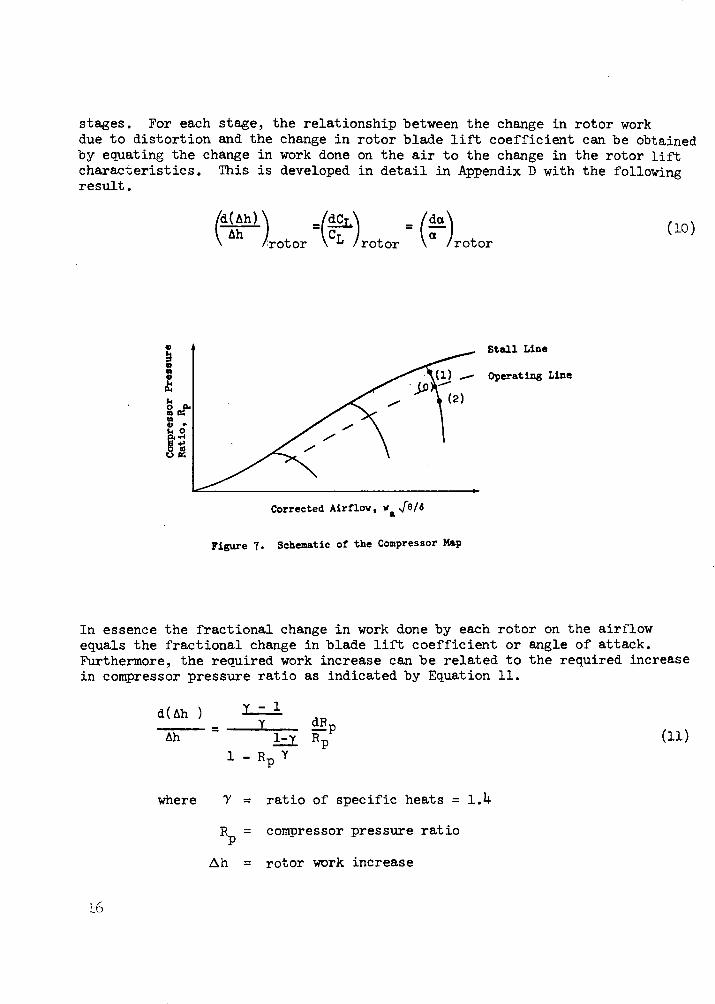
The overall performance of a compressor is represented by a compressor mapas shown schematically in Figure 7. To minimize weight, the engine is designedto operate at high stage loadings, near the stall line as shown. When thecompressor is subjected to a distorted flow, the average work done by thecompressor on the airflow remains constant, and corresponds to point 0 inFigure 7. However, that section of the compressor operating in the region oflow inlet total pressure must operate at a higher pressure ratio (point 1 inFigure 7) to pump the flow to the uniform compressor exit pressure. Theopposite condition holds for the high pressure regions, which correspond topoint 2 in Figure 7. The low pressure regions are of prime interest since theytend to reduce the compressor stall margin. The additional work required inthe low pressure regions is assumed to be evenly divided among the compressor
15
stages. For each stage, the relationship between the change in rotor workdue to distortion and the change in rotor blade lift coefficient can be obtainedby equating the change in work done on the air to the change in the rotor liftcharacteristics. This is developed in detail in Appendix D with the followingresult.
(CL )rotor /drotor
Stall Line
(1 Operating Line
0~
Corrected Airflow, wa e/6
Figure 7. Schematic of the Compressor Map
In essence the fractional change in work done by each rotor on the airflowequals the fractional change in blade lift coefficient or angle of attack.Furthermore, the required work increase can be related to the required increasein compressor pressure ratio as indicated by Equation 11.
d(Ah ) Y - 1= dRp
Th - 1 1-1 Rp- 1 - Rp ¥
where 7 = ratio of specific heats = 1.4
Rp = compressor pressure ratiop
Ah = rotor work increase
/d(Ah)
k~" )rotor
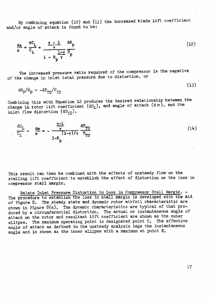
By combining equation (10) and (11) the increased blade lift coefficientand/or angle of attack is found to be:
da dCL y - 1 dR (12)L C (12)a CL YI¥ 1-y R
l - R P
The increased pressure ratio required of the compressor is the negativeof the change in inlet total pressure due to distortion, or
dRp/R = -dPT2/PT2 (13)
Combining this with Equation 12 produces the desired relationship between thechange in rotor lift coefficient (dCL), and angle of attack (d a), and theinlet flow distortion (dPT2).
dCL da dPT2 (14)
*L = - - .XPT21-R
P
This result can then be combined with the effects of unsteady flow on thestalling lift coefficient to establish the effect of distortion on the loss incompressor stall margin.
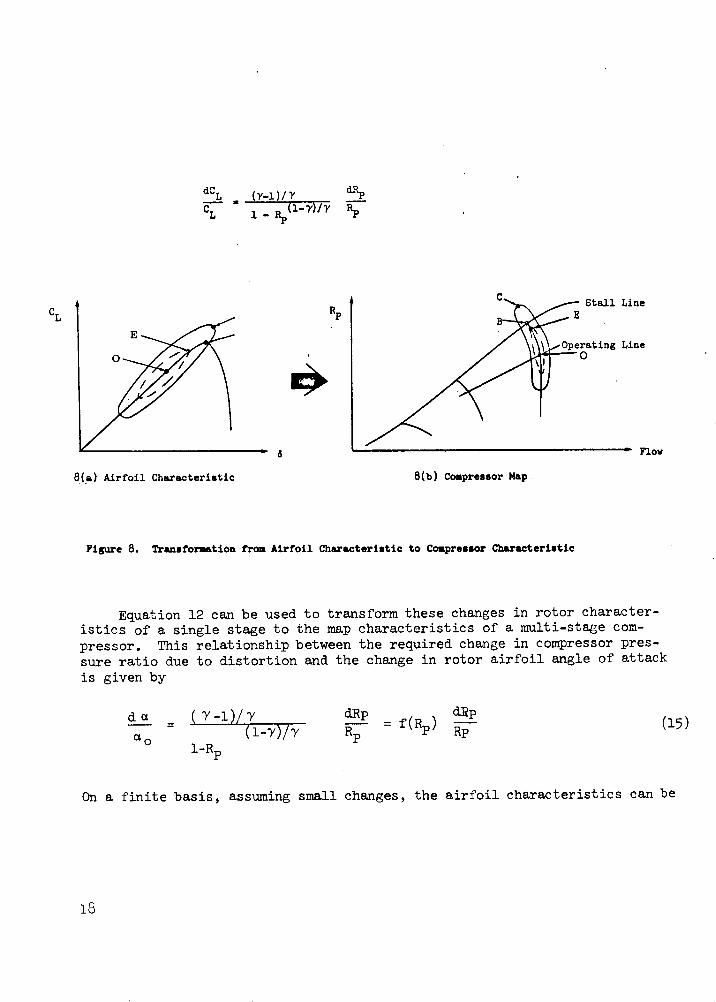
Relate Inlet Pressure Distortion to Loss in Compressor Stall Margin. -The procedure to establish the loss in stall margin is developed with the aidof Figure 8. The steady state and dynamic rotor airfoil characteristic areshown in Figure 8(a). The dynamic characteristics are typical of that pro-duced by a circumferential distortion. The actual or instantaneous angle ofattack on the rotor and resultant lift coefficient are shown as the outerellipse. The maximum operating point is designated point C. The effectiveangle of attack as defined in the unsteady analysis lags the instantaneousangle and is shown as the inner ellipse with a maximum at point E.
17
dCL -)/ Y dR
L 1 _ (l- y)/YCL 1 ,(- Rp I
a
8 (a) Airfoil Characteristic 8(b) Compressor Map
Figure 8. Transformation from Airfoil Characteristic to Compressor Characteristic
Equation 12 can be used to transform these changes in rotor character-istics of a single stage to the map characteristics of a multi-stage com-pressor. This relationship between the required change in compressor pres-sure ratio due to distortion and the change in rotor airfoil angle of attackis given by
( T-l)/ya 0 (1-y)/Y
dRp= f(Rp)
RP
dRpRp (15)
On a finite basis, assuming small changes, the airfoil characteristics can be
CLLine
Line
Flow
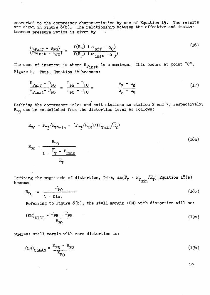
converted to the compressor characteristics by use of Equation 15. The resultsare shown in Figure 8(b). The-relationship between the effective and instan-taneous Pressure ratios is given by
(Rpeff - Rpo) =-Pinst - RpoJ
f(Rp) ( -eff - 0)
f(Rp)- (G inst - O )
The case of interest is where RPinst is a maximum.
Figure 8. Thus, Equation 16 becomes:
This occurs at point "C",
Rpeff - Rpo
Rpinst Rpo
RpE - Rpo
RPC - Rpo
aE - aC0ao - a
0
0(17)
Defining the compressor inlet and exit stations as station 2 and 3, respectively,RPC can be established from the distortion level as follows:
RPC T3/PT2min= (PT3 T2)/(PTmin / T)
(18a)
PC =1 - PT - PTmin
T
Defining the magnitude of distortion, Dist, as(fT - PT in/T),Equation 18(a)becomes min
Rpo(18b)
1 - Dist
Referring to Figure 8(b), the stall margin (SM) with distortion will be:
(SM)DIST = PB - PE
RPO
whereas stall margin with zero distortion is:
(SM)LEAN= Rp- Rpo
Rp0
(16)
(19a)
(19b)
19
RpO
RPC =
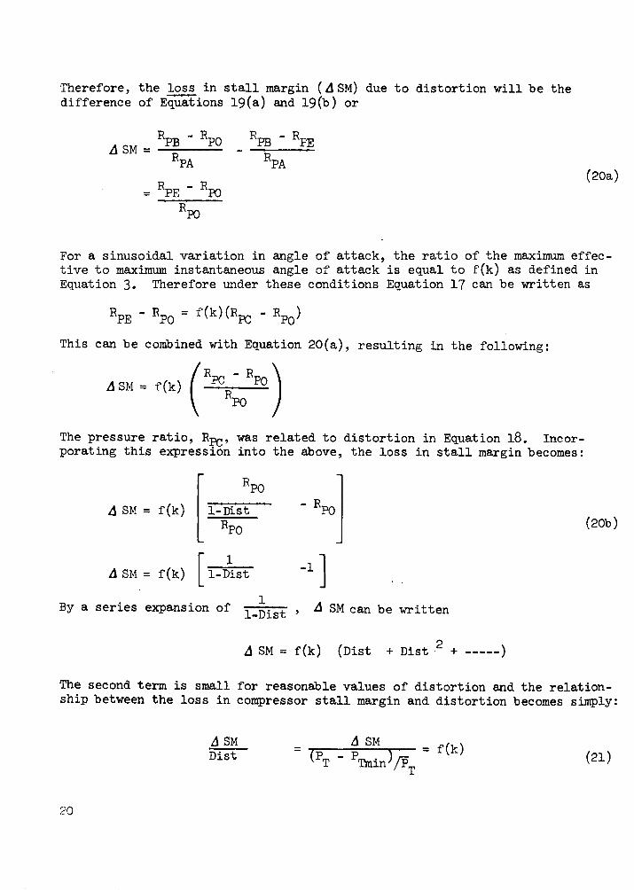
Therefore, the loss in stall margin (A SM) due to distortion will be thedifference of Equations 19(a) and 19(b) or
RpB - Rp0A SM =PB P0
RPA
= RpE - RP0
Rpo
RpB -RPE
RPA(20a)
For a sinusoidal variation in angle of attack, the ratio of the maximum effec-tive to maximum instantaneous angle of attack is equal to f(k) as defined inEquation 3. Therefore under these conditions Equation 17 can be written as
RPE - Rpo = f(k)(RPC -Rp0 )
This can be combined with Equation 20(a), resulting in the following:
ASIA = f(k) (ER %)Rpo
The pressure ratio, Rpc, was related to distortion in Equation 18. Incor-porating this expression into the above, the loss in stall margin becomes:
A SM = f(k)
Rp-
1-DistRp0
A SM = f(k) [1-Dist
- Rpo
-1 I
By a series expansion of 1Dist SM can be written
A SM = f(k) (Dist + Dist 2 + -----)
The second term is small for reasonable values of distortion and the relation-ship between the loss in compressor stall margin and distortion becomes simply:
A SMDist
a SM f(k)
T Tmin/_T f (21)
20
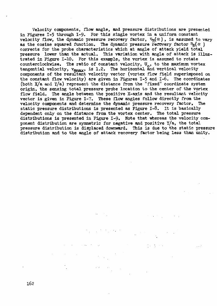
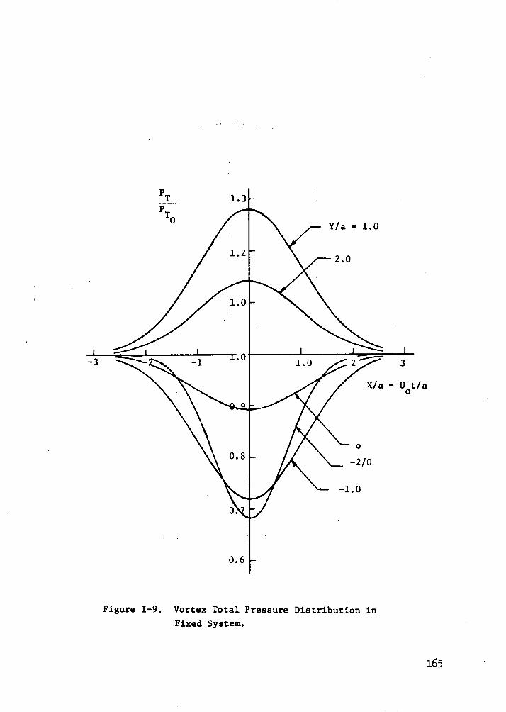
The loss in compressor stall margin can be established by use of Equation21 for a 180 degree sinusoidal circumferential distortion pattern. Results ofthis computation are shown in Figure 9 for T
1= T2 and for various values of
the non-dimensional time constant. The abscissa has been modified to includethe number of lobes, n, in the circumferential distortion pattern. The graphis thus generalized to enable the stall margin loss to be found for a com-pressor of reduced frequency, kc = U c/2U and for single or multiple lobedistortion patterns. This loss for several typical distortion patterns isshown in Figure 10 for three assumed compressors having reduced frequencies,kc, of 0.05, 0.10 and 0.15, respectively, and time constants r1 = 72 = 3.5.
1.0
.3." 4.
Z.01 .1 1.0
MODIFIED REDUCED FREQUENCY, k-nk "nu c/(2U)c c
Figure 9 The Effect of Compressor Reduced Frequencyand System Time Constants on Loss in Normalized
Compressor Stall Margin
1.o0
1r72'3.5
Z'-
I .5 1 ·# .r .05
.10
P4 P,~~~~~~~~ .15
IIN
1/REV 2/REV 3/REV 4/REV
Figure 10 Tolerance to Sinusoidal Distortion forDifferent Compressors
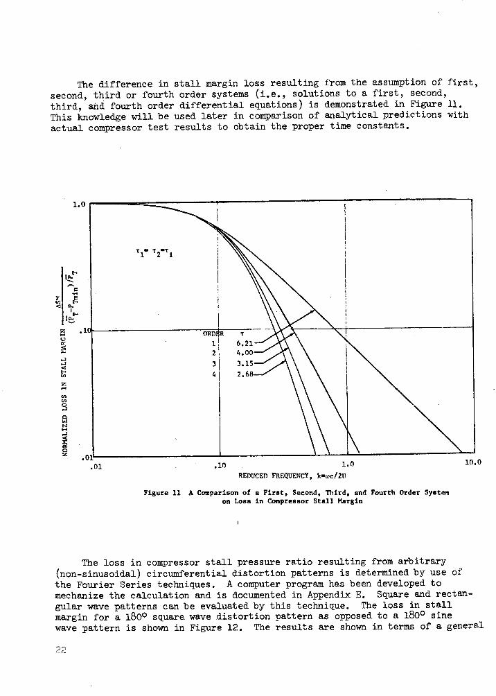
The difference in stall margin loss resulting from the assumption of first,second, third or fourth order systems (i.e., solutions to a first, second,third, and fourth order differential equations) is demonstrated in Figure 11.This knowledge will be used later in comparison of analytical predictions withactual compressor test results to obtain the proper time constants.
1.0
IN.
h
'.a
la
Z
r<.:
I
2:
It.
(n
To
0
UW
'-4
0z.
.01 .10 1.0 10.0
REDUCED FREQUENCY, k-wc/211
Figure 11 A Comparison of a First, Second, lTird, and Fourth Order Systemon Loss in Compressor Stall Margin
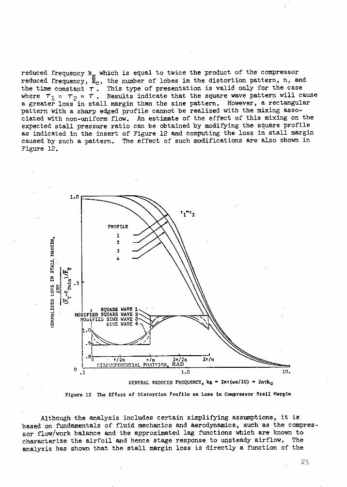
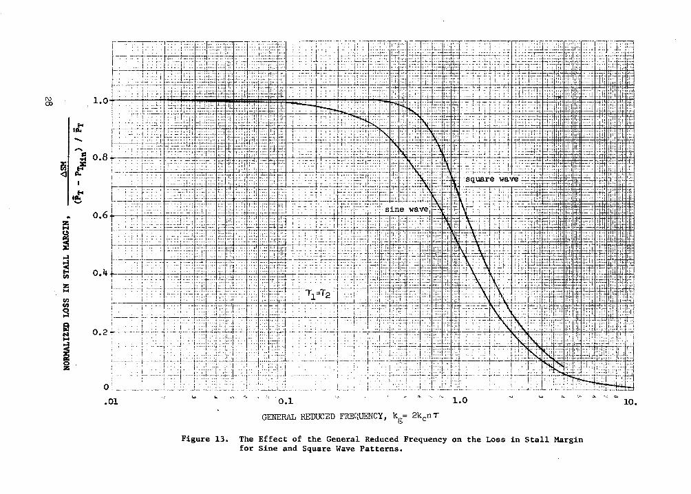
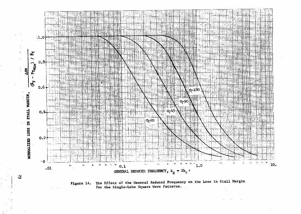
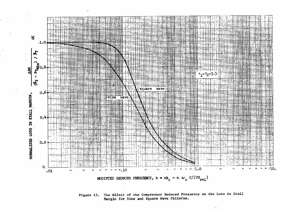
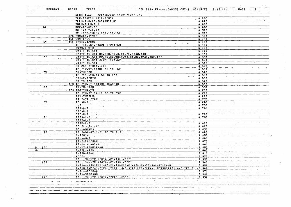
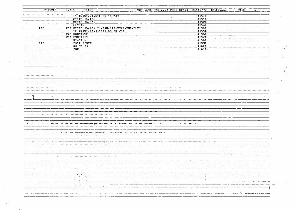
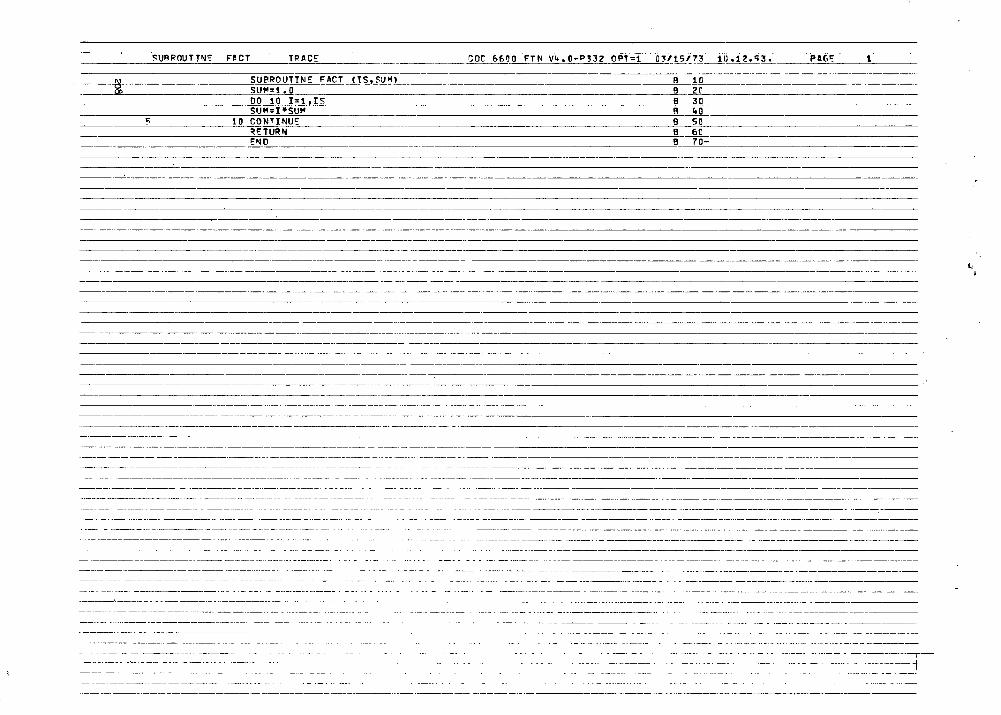
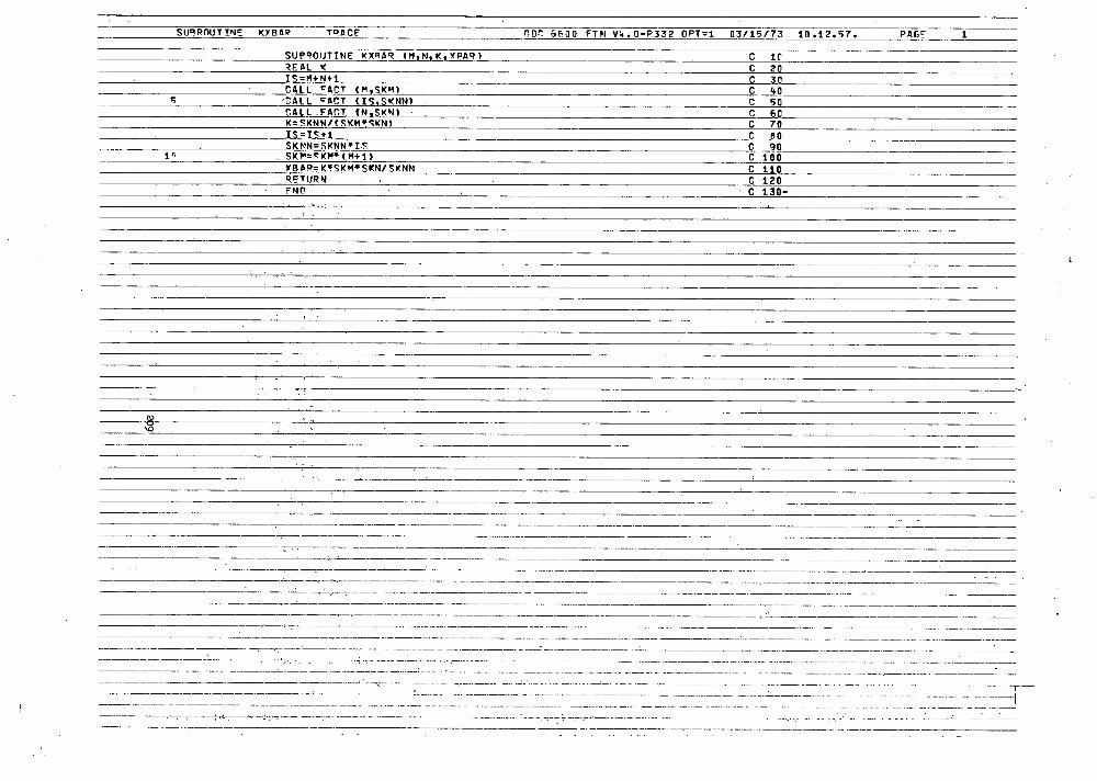
The loss in compressor stall pressure ratio resulting from arbitrary(non-sinusoidal) circumferential distortion patterns is determined by use ofthe Fourier Series techniques. A computer program has been developed tomechanize the calculation and is documented in Appendix E. Square and rectan-gular wave patterns can be evaluated by this technique. The loss in stallmargin for a 1800 square wave distortion pattern as opposed to a 1800 sinewave pattern is shown in Figure 12. The results are shown in terms of a general
reduced frequency k which is equal to twice the product of the compressorreduced frequency, k, the number of lobes in the distortion pattern, n, andthe time constant T. This type of presentation is valid only for the casewhere 7
1= = 2 = Results indicate that the square wave pattern will cause
a greater loss in stall margin than the sine pattern. However, a rectangularpattern with a sharp edged profile cannot be realized with the mixing asso-ciated with non-uniform flow. An estimate of the effect of this mixing on theexpected stall pressure ratio can be obtained by modifying the square profileas indicated in the insert of Figure 12 and computing the loss in stall margincaused by such a pattern. The effect of such modifications are also shown inFigure 12.
1.0
z
0
v.1E.4 IAZH rI1
.1 1.0 10.
GENERAL REDUCED FREQUENCY, kg - 2nr(wc/2U) - 2nxkc
Figure 12 The Effect of Distortion Profile on Loss in Compressor Stall Margin
Although the analysis includes certain simplifying assumptions, it is
based on fundamentals of fluid mechanics and aerodynamics, such as the compres-
sor flow/work balance and the approximated lag functions which are known tocharacterize the airfoil and hence stage response to unsteady airflow. The
analysis has shown that the stall margin loss is directly a function of the
23
distortion level ((PT - PTmin)/T), the shape of the distortion pattern and ofthe compressor rotor reduced frequency, kc.
Application and Generalized Curves
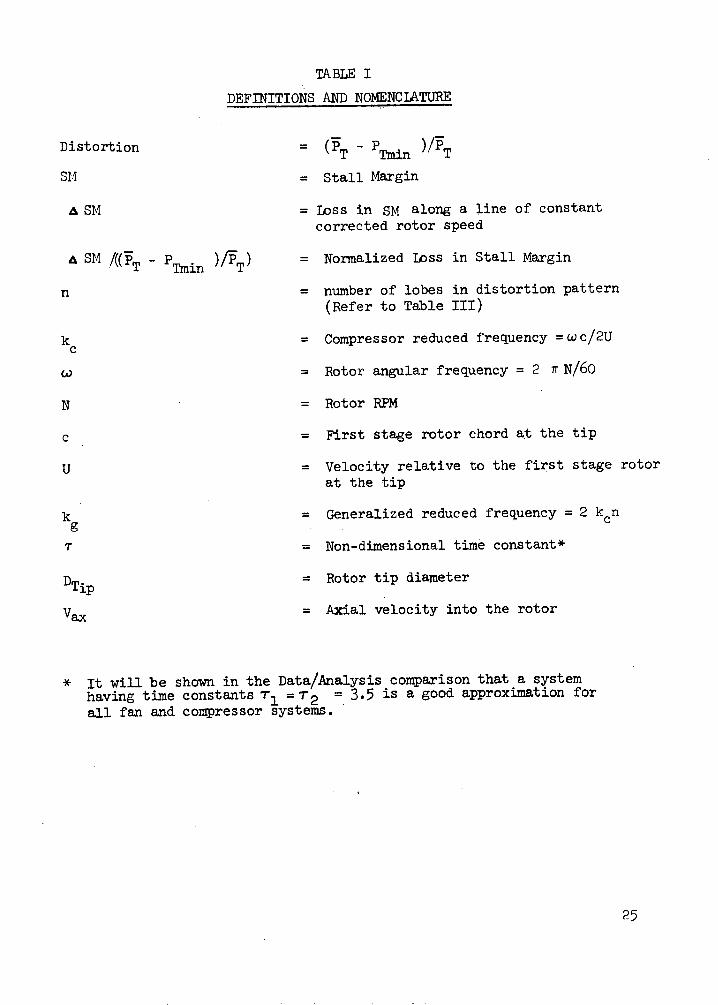
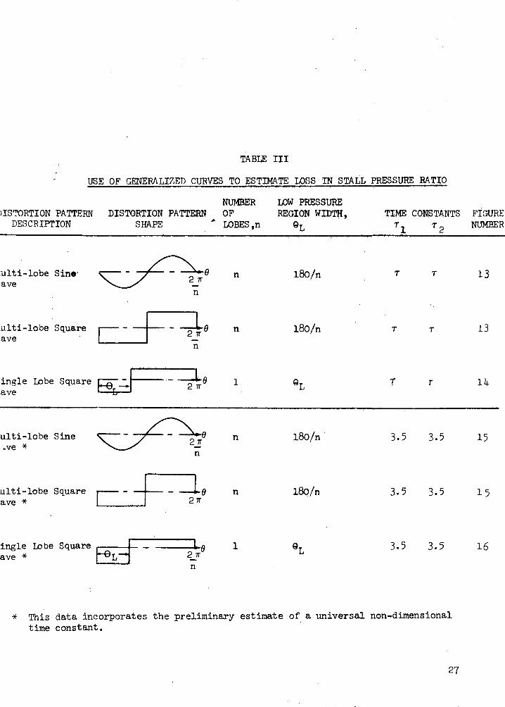
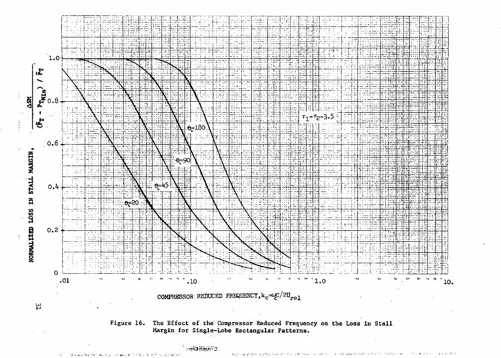
The technique relating arbitrary circumferential distortion patterns tothe loss in compressor stall pressure ratio has been established. This analy-sis has been computerized. Documentation and instructions for use of thisprogram is given in Appendix E. However, many inlet distortion patterns canbe approximated by standard patterns of sine or rectangular wave shape.Furthermore, the loss in stall margin resulting from such distortion patternsis basically dependent upon only the extent of the low pressure region, QL, therotor time constant, 7, and the rotor reduced frequency, kc. As a result, theloss in stall margin associated with these patterns can be presented as afunction of these three variables, QL, r , and kc. Therefore a set of general-ized curves have been compiled that can be readily used to estimate the lossin compressor stall margin for these standard patterns.
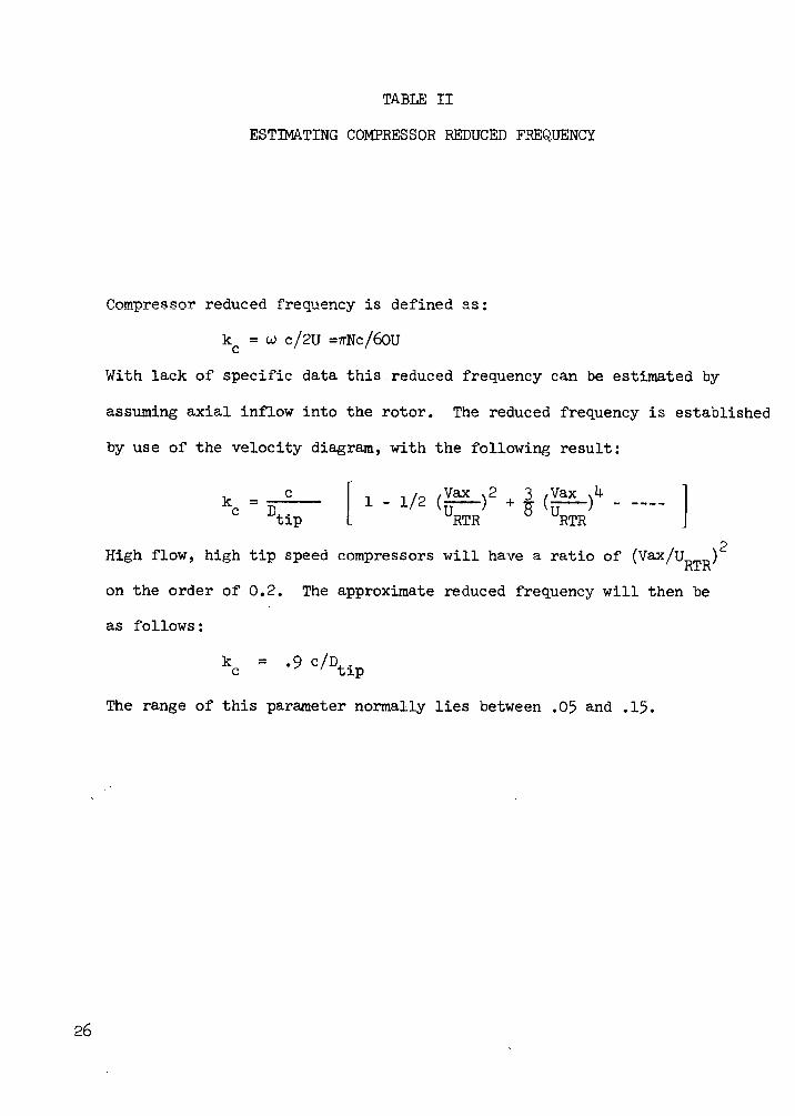
The three basic distortion patterns utilized to compile the generalizedcurves are shown in Table III. Applicable definitions and nomenclature arepresented in Table I as an aid in estimating the loss in stall pressure ratiofor those patterns defined in Table III. A means to approximate the compressorreduced frequency is shown in Table II.
Table III is composed of two parts. The curves outlined in the first partare completely general and can be used with a non-dimensional time constantchosen by the user to establish, for example, the effect of different timeconstants on a comparison between the analysis and a specific set of compressortest data. The second part pertains to those generalized curves utilizing afixed non-dimensional time constant with a value of T = 3.5. It will be shownin the Data/Analysis Comparison that this constant will produce a good matchbetween test results and the analysis. The specific curve applicable to agiven problem will depend on the distortion pattern and available informationon the non-dimensional time constant. Table III is intended to give therequired guidance for use of the specific curves, contained in Figures 13through 16.
Comparison of Analysis with Test Data
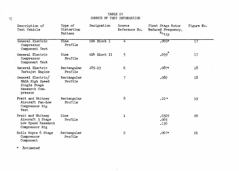
A limited comparison between results of the analysis with test data wasconducted to add credence to the analysis developed herein, which is basedsolely on theoretical grounds. A literature search was conducted and the datalimited to that readily available in published sources. Much of this datalacks specific details and the reduced frequency of the respective turbo-machinery has been estimated. A description of each test vehicle along withthe source of information and the reduced frequency is given in Table IV.
The data comparison is made assuming a single non-dimensional time con-stant to be valid for all turbomachinery. In such a case the compressor
24
TABLE I
DEFINITIONS AND NOMENCLATURE
Distortion
SM
a SM
A SM /((PT - Tmin )/ T)
n
kC
N
c
U
kg
DTip
Vax
= (PT -Tmin )/ T
= Stall Margin
= Loss in SM along a line of constantcorrected rotor speed
= Normalized Loss in Stall Margin
= number of lobes in distortion pattern(Refer to Table III)
= Compressor reduced frequency = wc/2U
= Rotor angular frequency = 2 7 N/60
= Rotor RPM
= First stage rotor chord at the tip
= Velocity relative to the first stage rotorat the tip
= Generalized reduced frequency = 2 ken
= Non-dimensional time constant*
= Rotor tip diameter
= Axial velocity into the rotor
* It will be shown in the Data/Analysis comparison that a systemhaving time constants 71 = r
2= 3.5 is a good approximation for
all fan and compressor systems.
25
TABLE II
ESTIMATING COMPRESSOR REDUCED FREQUENCY
Compressor reduced frequency is defined as:
kc= w c/2U =frNc/60U
With lack of specific data this reduced frequency can be estimated by
assuming axial inflow into the rotor. The reduced frequency is established
by use of the velocity diagram, with the following result:
c = c [ 1 - 1/2 ( 2 + Vax 4 c Dtip [ URTR+ 7 URTR
High flow, high tip speed compressors will have a ratio of (Vax/U )2
on the order of 0.2. The approximate reduced frequency will then be
as follows:
k = .9 c/Dti p
The range of this parameter normally lies between .05 and .15.
26
TABLE III
USE OF GENERALIZED CURVES TO ESTIMATE LOSS IN STALL PRESSURE RATIO
DISTORTION PATTERNDESCRIPTION
DISTORTION PATTERNSHAPE
NUMBEROFLOBES,n
LOW PRESSUREREGION WIDTH,
0L
TIME
T
ulti-lobe Sine'ave
ulti-lobe Squareave
ingle Lobe Squareave
2ir
n
l-_- Le 2i
n
ulti-lobe Sine.ve *
ulti-lobe Squareave *
ingle Lobe Squareave *
2rn
Le
2r
n
n 18 0/n
n 180/n
1 97
3.5 3.5
3.5 3.5
3.5 3.5
* This data incorporates the preliminary estimate of a universal non-dimensionaltime constant.
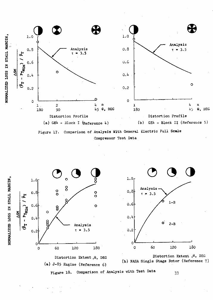
Distortion Profile Distortion Profile(a) GE4 - Block I (Reference 4) (b) GE4 . Block II (Reference 5)
Figure 17. Comparison of Analysis With General Electric Full Sc4le
Compressor Test Data
o
o oo
oo 0o 0
0
0
Analysis
T '3.5
1.0
0.8
0.6
0.4
1-B
O 2-B
0 60 120 180 0 60 120 180
Distortion Extent ,O, DEG Distortion Extent ,G, DEG(a) J-85 Engine (Reference 6) (b) NASA Single Stage Rotor (Reference 7)
Figure 18. Comparison of Analysis with Test Data 33
3 :1.0
0.8E4
0.6
0.4X 0.4I
lPA% 0.2
0
1.0r
C1
O'4zj-4
I104
%14
0
) O O
1:' 1Z
ANALYSIS 00
1.0
0.8
0. 6
0.4
0.2
0
0
0
60 120 180
DISTORTION EXTENT, 0, DEG
1180
2 390 60
DISTORTION PROFILE
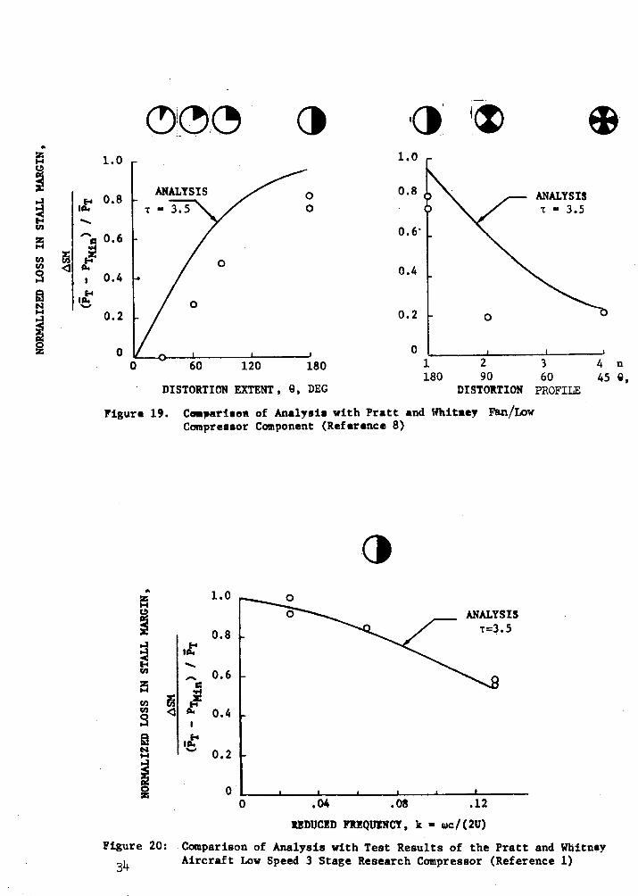
Ceparison of Analysis with Pratt and Whitney Fan/LowCompressor Component (Reference 8)
0
ANALYSIST=3.5
.08 .12
REDUCED FREQUENCY, k - wc/(2U)
Figure 20: Comparison of Analysis with Test Results of the Pratt and Whitney34 Aircraft Low Speed 3 Stage Research Compressor (Reference 1)
ciI
A
zU]
.
laNN
9
1.0
,o 0.8
A 0.6
14
10.4
0.2
00
Figure 19.
4 n45 0,
C1.0
in
IzNI.
14
lt
'A'
E
06
14IA64
0.8
0.6
0.4
0.2
o L0
000
cc�oO
O 1.0
o
ANALYSIST = 3.5
0.6,
0.4
0.2
O00 60
DISTORTION EXTENT, 0, DEG
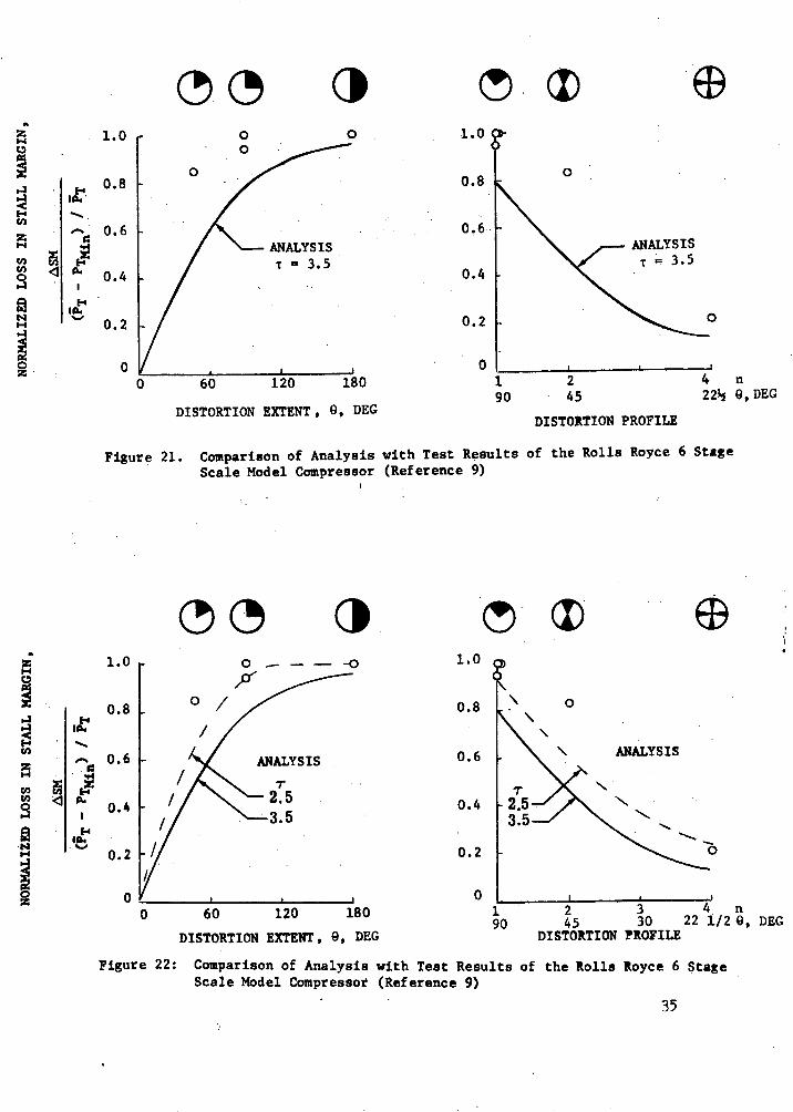
Comparison of Analysis with Test ResultsScale Model Compressor (Reference 9)
o
ANALYSIST = 3.5
0
90 45
DISTORTION PROFILE
of the Rolls Royce 6 Stage
cz3
00 60 120
1.0
0.8
0.6
0.4
0.2
0180
DISTORTION EXTENT, 9, DEG
o
\ANALYSIS
<\\'"
90 45 30DISTORTION PROFILE
4 n22 1/2 9, DEG
Comparison of Analysis with Test ResultsScale Model Compressor (Reference 9)
of the Rolls Royce 6 Stage
35
1.01.4
1
PA
zH
o
Z
0
N
H
0.8
0.6
0.4
0.2
r.
"4IA.
,£
0
Figure 21.
4 n22½ , DEG
1.0
1*4
A.
14IA.
0.8
0.6
0.4
0.2
Figure 22:
q)
(0( (n '
Om
sensitivity to distortion is dependent only on the rotor reduced frequencyas shown earlier (Effect of Inlet Pressure Distortion on Loss in Stall PressureRatio). The comparison is presented in terms of the normalized loss in stallpressure ratio in Figures 17 through 21 for the constant non-dimensional timeconstant of 3.5. Without exception, the trends predicted by use of the analy-sis are in very good agreement with results of the tests, and in many cases,good quantitative agreement is obtained. (See for example Figure 20)
The non-dimensional time constant of 3.5 was assumed universally appli-cable in the above comparison. As shown it produces reasonable agreement withdata and as a result is recommended for use during the development phase of aninlet/engine program. However, the analysis also provides the mechanism toimprove data/analysis comparison once test data of production type hardwareis available. For example, the prediction shown in Figure 21 for T = 3.5 canbe modified by assuming a time constant, T = 2.5, bringing the analysis inexceptionally close agreement with the test results as shown in Figure 22.This further demonstrates the validity of the basic approach.
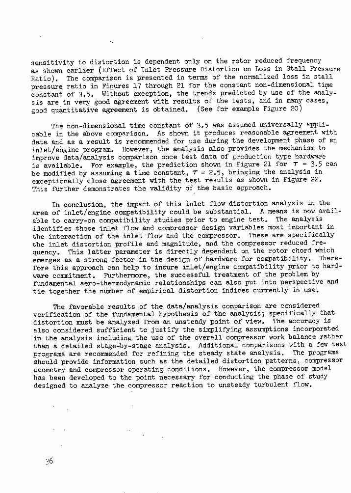
In conclusion, the impact of this inlet flow distortion analysis in thearea of inlet/engine compatibility could be substantial. A means is now avail-able to carry-on compatibility studies prior to engine test. The analysisidentifies those inlet flow and compressor design variables most important inthe interaction of the inlet flow and the compressor. These are specificallythe inlet distortion profile and magnitude, and the compressor reduced fre-quency. This latter parameter is directly dependent on the rotor chord whichemerges as a strong factor in the design of hardware for compatibility. There-fore this approach can help to insure inlet/engine compatibility prior to hard-ware commitment. Furthermore, the successful treatment of the problem byfundamental aero-thermodynamic relationships can also put into perspective andtie together the number of empirical distortion indices currently in use.
The favorable results of the data/analysis comparison are consideredverification of the fundamental hypothesis of the analysis; specifically thatdistortion must be analyzed from an unsteady point of view. The accuracy isalso considered sufficient to justify the simplifying assumptions incorporatedin the analysis including the use of the overall compressor work balance ratherthan a detailed stage-by-stage analysis. Additional comparisons with a few testprograms are recommended for refining the steady state analysis. The programsshould provide information such as the detailed distortion patterns, compressorgeometry and compressor operating conditions. However, the compressor modelhas been developed to the point necessary for conducting the phase of studydesigned to analyze the compressor reaction to unsteady turbulent flow.
TASK IIFLUID DYNAMIC MODEL OF TURBULENT INLET FLOW
Turbulent flow produced in an aircraft inlet system can result inmomentary total pressure distortion levels of a magnitude and durationsufficient to cause engine compressor stall. The first attempt to identifysuch instantaneous distortion levels was in terms of the Root Mean Square (RMS)level and the Power Spectral Density (PSD) function of the total pressurefluctuations. These statistical averages are relatively inexpensive to obtain.However, no physical interpretation could be given such quantities and as aresult were of little value in the correlation of unsteady flow and compressorstall. Presently, it is common practice to measure an instantaneous distortionpattern at each instant of time by use of high response, highly (time) corre-lated total pressure instrumentation. This requires complex and expensivedata measurement systems. While these instantaneous patterns graphicallydemonstrate the existence of unsteady flow, only limited empirical correlationsof unsteady flow and compressor stall have been shown. The high cost of datareduction severely restricts the quantity of data analysis that can be made tosubstantiate any correlation. In addition, an empirical approach is inherentlyweak since it does not provide physical understanding of the basic flow phe-nomena. An analysis relating turbulent flow phenomena in the inlet to com-pressor stall is required.
A fluid dynamic model of turbulent flow is developed herein as a meansof understanding turbulent inlet flow and as a practical tool for evaluatingflow properties through the use of the total pressure RMS level and PSD func-tions. By use of this flow model, which is based on a combination of basicfluid dynamic concepts and statistical analyses, a better understanding of themechanics of the flow is obtained. Consequently, the loss in compressor stallmargin may ultimately be related to the statistical characteristics of turbu-lence.
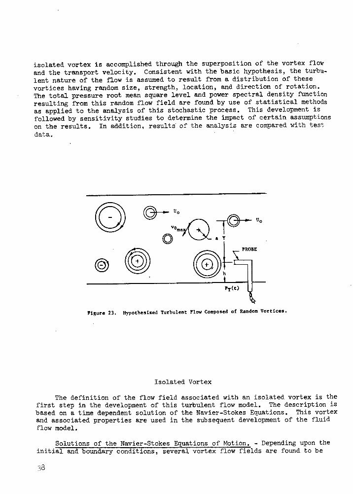
The approach used to analyze this turbulent flow is outlined below andpresented in detail in the subsequent sections of the report. Turbulence,normally measured in terms of velocity or total pressure, implies pressuregradients exist in the flow. It is a fundamental of fluid mechanics thatpressure gradients can be supported by only two means: (1) pressure wavestraveling at (or above) the local sound speed and (2) by streamline curvature.Since turbulence is produced by viscous phenomena, it is proposed that thepressure fluctuations measured in an inlet are primarily supported by stream-line curvature. To realistically model the flow, it is hypothesized that thestreamline curvature and resultant pressure fluctuations are caused by arandom distribution of discrete vortices being convected downstream by themean flow. This is illustrated schematically in Figure 23.
To obtain a mathematical representation of this flow model, a coordinatesystem moving downstream with the mean flow is used and enables the individualvortices to be analyzed in a steady frame of reference. Steady state flowequations can then be applied to describe the flow field about an isolatedvortex. Analytical construction of the total pressure signature of this
37
isolated vortex is accomplished through the superposition of the vortex flowand the transport velocity. Consistent with the basic hypothesis, the turbu-lent nature of the flow is assumed to result from a distribution of thesevortices having random size, strength, location, and direction of rotation.The total pressure root mean square level and power spectral density functionresulting from this random flow field are found by use of statistical methodsas applied to the analysis of this stochastic process. This development isfollowed by sensitivity studies to determine the impact of certain assumptionson the results. In addition, results of the analysis are compared with testdata.
(e.- Uo
a Y
I _ PROBE
PT(t)
Figure 23. Hypothesized Turbulent Flow Composed of Random Vortices.
Isolated Vortex
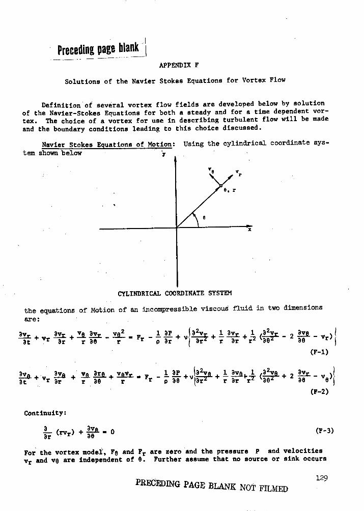
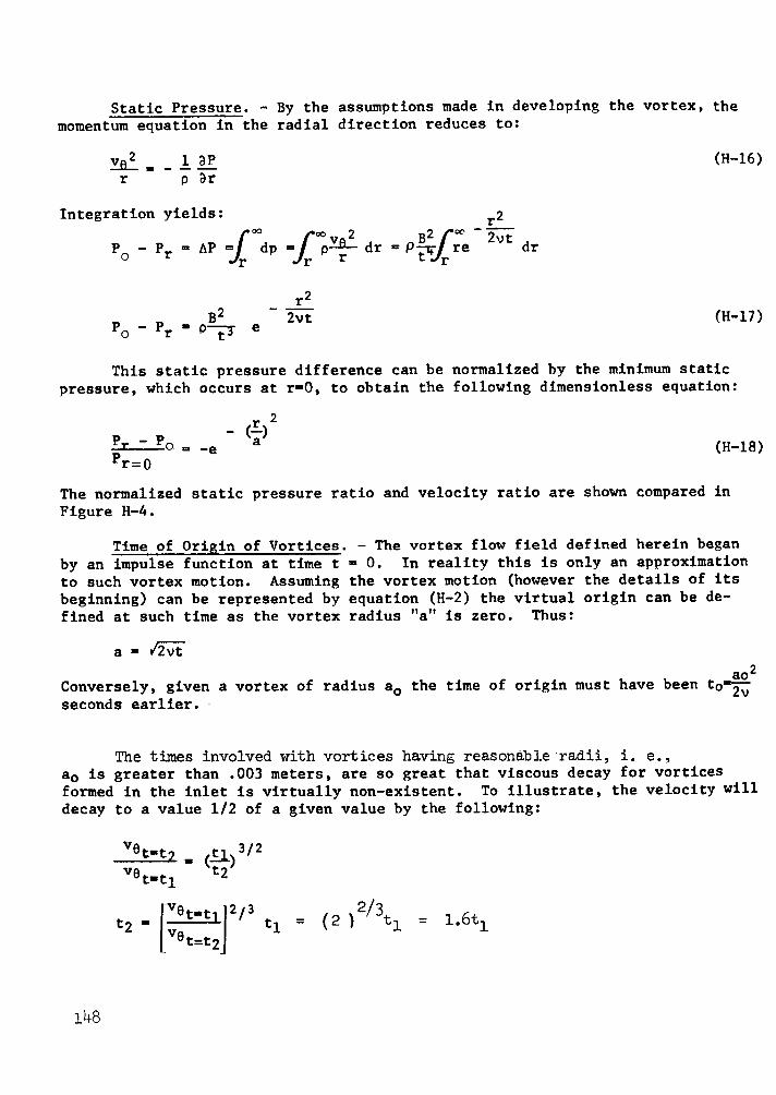
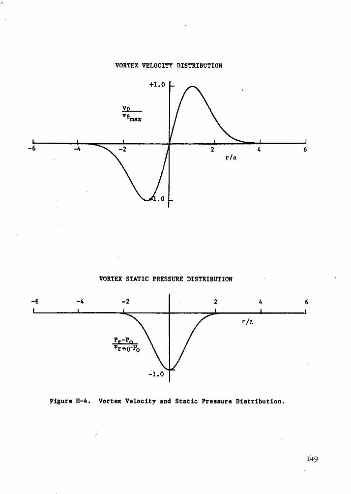
The definition of the flow field associated with an isolated vortex is thefirst step in the development of this turbulent flow model. The description isbased on a time dependent solution of the Navier-Stokes Equations. This vortexand associated properties are used in the subsequent development of the fluidflow model.
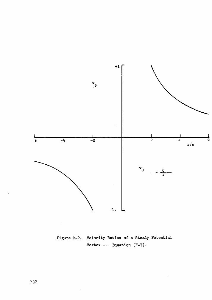
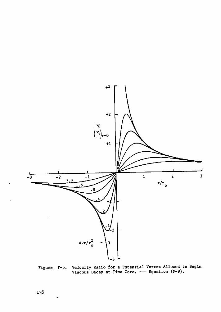
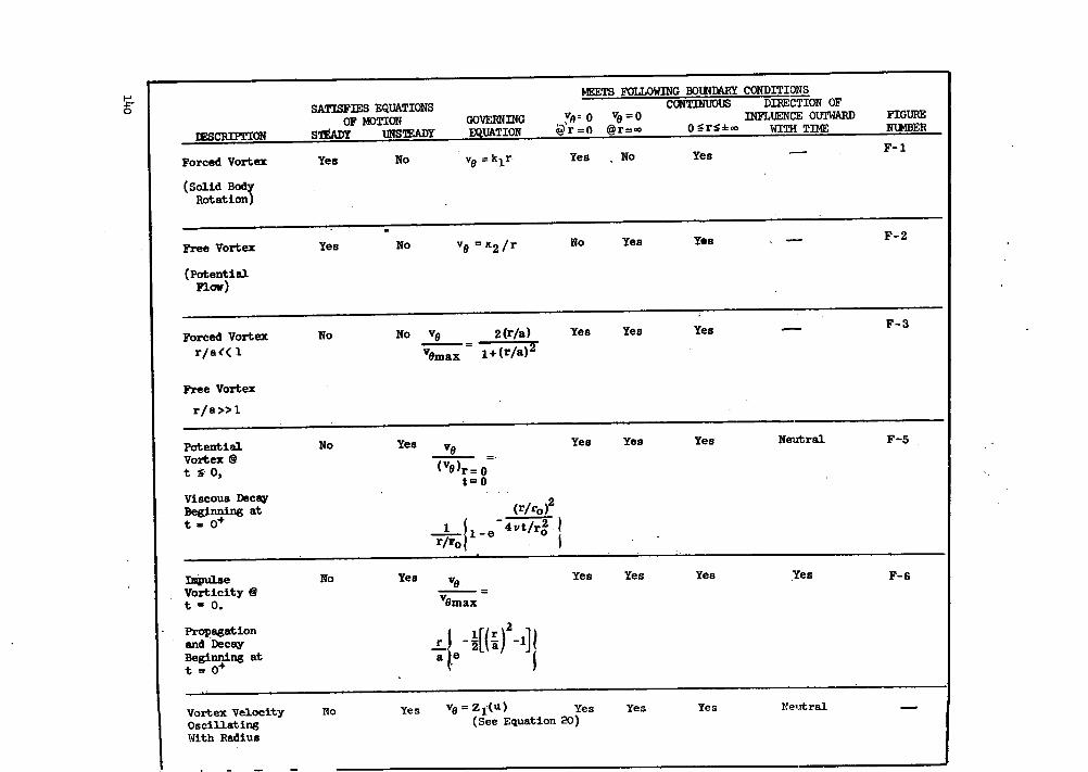
Solutions of the Navier-Stokes Equations of Motion. - Depending upon theinitial and boundary conditions, several vortex flow fields are found to be
:8
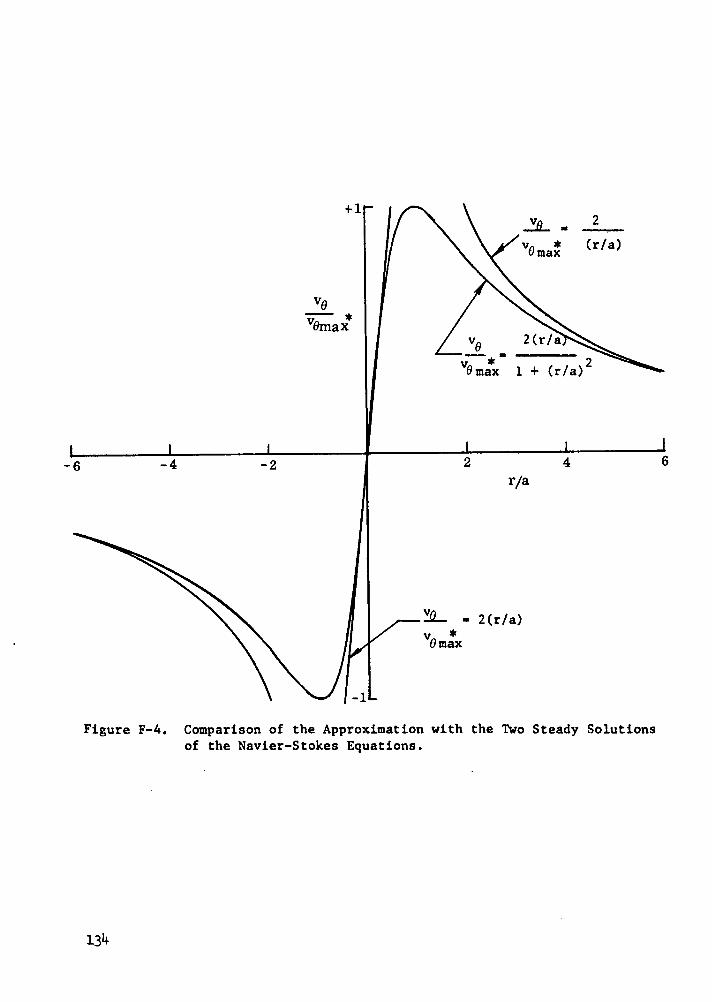
0
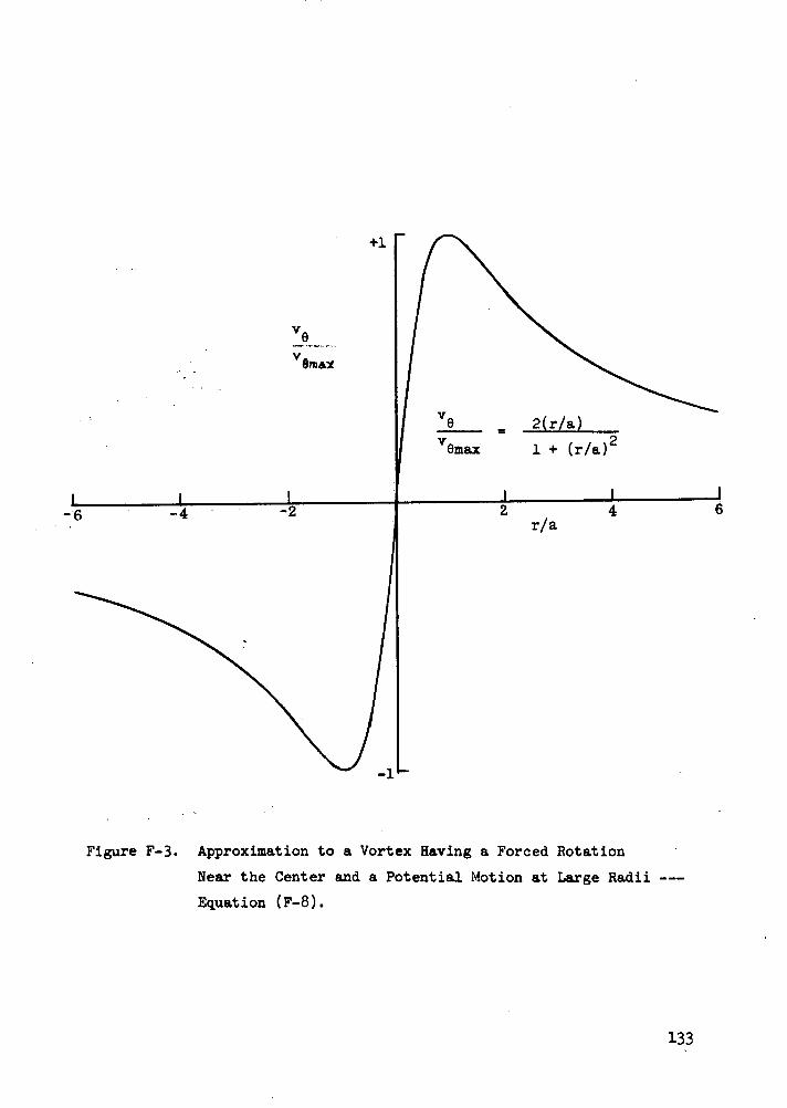
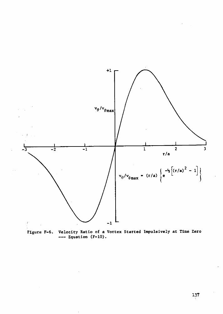
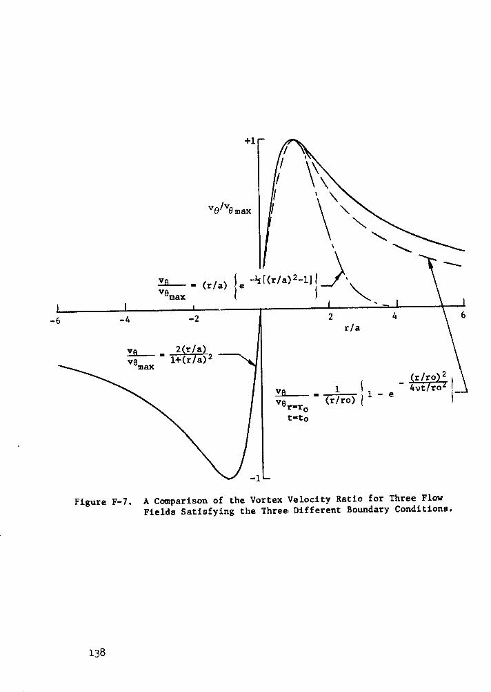
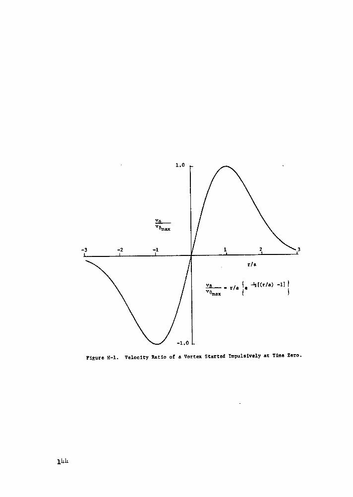
solutions of the Navier-Stokes Equations. The details and the characteristicsof these solutions are presented in Appendix F. It was found that all steadystate solutions have singularities (infinite velocities) at either the vortexcenter or outer extremity and therefore do not represent real flows. There-fore, the time dependent solutions, each representing different vortex boundaryconditions, were examined. For a realistic flow, the solution must satisfy thefollowing boundary conditions: (1) the vortex must have a tangential velocityof zero at both the center and at an infinite radius, (2) the velocity must becontinuous for all radii, and (3) the influence of the vortex must move outwardwith time. The solution of the two-dimensional time dependent Navier-StokesEquations that fits these assumed boundary conditions is a vortex formed by animpulsive start in an undisturbed flow. The normalized velocity field asso-ciated with this vortex is given in Equation 22.
2
=n e 2 [(a) 2 (22)Vmax a
where vQ = velocity in the 0 direction (cylindrical coordinatesystem)
vgmax = maximum velocity of the given vortex at a given time
a = radius at which vO= vQmax
n = specifies direction of rotation, = 1 for counter-clockwise and -1 for clockwise
The radius r = a at which the velocity is a maximum is considered the vortexcore radius. This core radius varies with time and as a result, the influenceof this vortex increases in the radial direction with time.
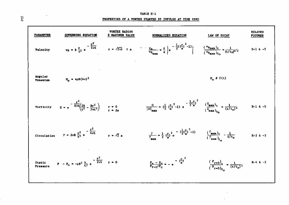
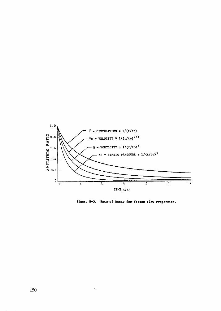
A complete development of this vortex is presented in Appendix H andincludes a description of the angular momentum, vorticity, circulation and adiscussion on the time of origin and decay of the vortex.
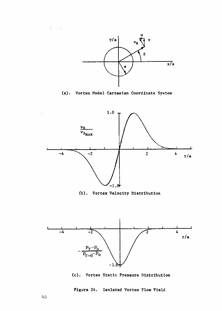
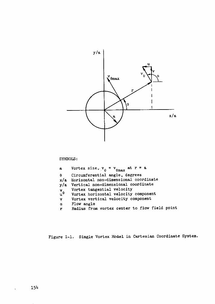
Vortex Description in Cartesian Coordinates. - In order to describe theproperties of the vortex in terms of a coordinate system fixed with respect tothe inlet it is first necessary to express the vortex properties in terms ofa Cartesian coordinate system fixed to the center of the vortex (x, y) asopposed to the cylindrical coordinate system (r, Q) used for solutions of theNavier-Stokes Equations. A description of the coordinate system used is shownin Figure 24(a).
As developed in Appendix H the circumferential velocity is a function ofthe radius and time and is given by Equation 23.
rBr (23)Br -4 (23)
ve '-rA e
39
U
y/a v
(a). Vortex Model Cartesian Coordinate System
1.0
vA
VOmax
-4 2 4 r/a
(b). Vortex Velocity Distribution
Pr-Po
Pr=0-Po
4r/a
(c). Vortex Static Pressure Distribution
Figure 24. Isolated Vortex Flow Field
where: B = constant depending on the vortex strength
v = kinematic viscosity
t = time since the vortex started.
However, due to the short period of time the vortex is in the field of interest(the inlet duct) and the very slow rate of growth of the vortex, the time isassumed constant. The vortex tangential velocity normalized by the maximumvelocity, which occurs at r = a, was given by Equation 22 and repeated below.The variation of vg with r is shown in Figure 24(b).
- [(r/a) 2-1]ve - n(r/a) e (22)
rOmax
The horizontal (u) and vertical (v) velocity components of the vortexvelocity are obtained by use of the description and definitions of the coordi-nate systems of Figure 24(a). These are:
nYa) - [(x/a) 2+(y/a) 2l1]u ' -~Vmax(Y/a) e
-½ [(x/a) 2+(y/a) 2-1 ]v - ven(x/a) e (25)
The local flow angle is dependent on the velocity components, and is given byEquation 26.
a - arctan (v/u) - arctan ( tan-) (26)
The static pressure variation with radius as determined in Appendix I is givenby Equation 27 and shown in Figure 24(c).
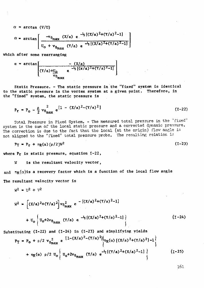
Pro =. 2 e - [(x/a)2 +(y/a)2-1]Pr- 2 Vemax e (27)
where: Pr = static pressure at radius r
Po = static pressure beyond the vortex influence,r>>a
P = density
The total pressure in the vortex flow field, based on a coordinate system fixedto the vortex center, is equal to the sum of static and dynamic pressures or
41
PT - Pr vo 2 (28)
In terms of the cartesian coordinate system, the total pressure is obtained bycombining Equations 22, 27, and 28 and is given by Equation 29.
PTpo -M P [(x/a)2 +(y/a)2-]vea e- [(x/a)2 +(y/a)2 -1] (29)
Transformation of the Vortex Flow Field to the Inlet Coordinate System. -The vortex flow field has been described in the coordinate system fixed to thevortex center. The vortex, however, is moving downstream at the local averageflow velocity. To determine the total pressure as it would be measured at theengine face, it is necessary to transform the vortex velocity field into thecoordinate system fixed to the inlet.
Allowing the vortex to move downstream at the local velocity, Uo, as shownin Figure 25, the local instantaneous velocity components as would be measuredin a coordinate system fixed at the probe becomes:
(30)U - Uvvme x(/a e - [(X/a) 2+(Y/a) 2- 1
V - -ve(X/a) e - [(X/a)2 +(y/a)2 -1(V -emax(Xa
Here, the upper case (X, Y) represent the position of the vortex center relativeto the origin of the fixed coordinate system located on the probe. In essence,U and V are the velocity components at the probe due to a vortex located at(X, Y). In this case, the transformation between the moving and fixed coordi-nate systems is simply
X = -x(32)
Y = -y
The static pressure in the fixed coordinate system is
- [(X/a) 2 +(y/a)2 -1]Pr -P Vemax e
(31)
(33)
VORTEX COORDINATESYSTEM
TOTAL PRESSURE PROBE
X
FIXED COORDINATE SYSTEM
Figure 25. Transformation of Coordinate Systems.
To account for the fact that the local flow angle at the total pressure probeis not aligned with the probe, the total pressure as expressed in Equation 34is assumed to be the local static pressure plus a corrected dynamic pressure.
PT ' Pr+naR(a)=2 (34)
where: Pr = static pressure (which is independent of coordinatesystem)
W = the resultant velocity vector, (U2 + V2)1 /2
7IR = probe total pressure recovery
a = local flow angle
Since the vortex is moving downstream at velocity U , the position, X, ofthe vortex center with respect to the fixed (probe) coordinate system is afunction of the velocity, Uo, and time, t. Thus:
x- Uot (35)
This implies that the origin of time must be chosen such that X = O when t = 0.
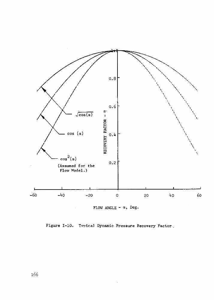
The total pressure recovery is assumed to vary directly by the square ofthe cosine of the flow angle, a , at the probe.
nR l COB2 -U)2 (36)(j7
43
H
I i II I III I III -I I I I I I I I I " 11 I ZI I I I� -II e I /Ji 1 I I / / /A L~/////L/ / / / *.. / I ../ ... / /
Using the transformation of Equation 35, the total pressure recovery, andthe definition of static pressure (Equation 33) and velocity (Equation 30 and31), the total pressure expressed by Equation 34 becomes:
PT-PTo= nPU 0 (-)e a (37)
+n 22 [(v/a)2 1] [(a a
where PT is the total pressure of the undisturbed flow and equal to
Po + p Uo2
Defining this delta pressure as A PT and normalizing by the dynamic pressure,
The resultant total pressure is a function of the time, t, the meanvelocity, UO, the strength of the vortex vGmax, the core size of the vortexa, and direction of rotation, n. Detailed development of these relation-ships are given in Appendix I.
Although these relations have been developed for a single vortex, they areapplicable to a series of vortices. These vortices can assume random valuesof size, strength, location and direction. In such a case the vortex proper-ties, a, vQmax, y, and n, become random variables. The techniques requiredto treat these properties as random variables are developed in Appendix J.These tools are then used in conjunction with Equation 39 to establish thestatistical characteristics (RMS and PSD) of the proposed flow field.
Statistical Flow Model
The model of turbulent inlet flow is hypothesized as being composed ofa random distribution of vortices, each having a specific size, strength,direction of rotation, and location as shown in Figure 23. The total pressure
fluctuation created by each vortex is given in Equation 39. For a specificvortex having a given set of properties, a, vomax, y, and n, Equation 39signifies a single time function. However, each vortex has a different set ofproperties; consequently, the flow field is composed of a family of timefunctions. This family is called a stochastic process.
The autocorrelation function and its Fourier Transform, the power spectraldensity function resulting from this process, are found in functional form bystatistical methods as applied to a general stochastic process in Appendix J.These developments are applied to the vortex flow field to obtain the totalpressure autocorrelation and power spectral density functions of the turbulence.The fluctuations in total pressure are also related to the fluctuations invelocity by use of the flow model, providing an analytical means to relate,hot wire anemometer velocity measurements and total pressure measurements.
Autocorrelation Function. - The autocorrelation function of the stochasticprocess composed of the random vortices flowing downstream with the flux of Nper second can be summarized as follows.
The general total pressure wave described by Equation 39 can be repre-sented by the following functional notation.
APT= APT (a,v,Y,n,t) (40)
The autocorrelation function of this discrete total pressure wave is found bymeans of the definition of the autocorrelation function and is given by
o00
R (av,v,(a,v.,Y= PT(a ,nt) APT(a,v,Y,n,t + t)dt (41)
_00
To establish the autocorrelation function of the entire family of waves, aweighted sum of the function RAP (a, v, Y, n, T) is performed over allpossible values of a, v, Y, and n. T The weighting functions are the percentageof vortices having a specific core size between a and a + Aa, specific strengthbetween vomax and vemax + Avemax, a specific location between y and y +Ay anda direction of rotation (n = +1 or -1). These weighting functions are assumedindependent of each other, are simply the probability density functions of a, v,y, and n, respectively, and are designated by the notation, p( ). The auto-correlation function of the resultant total pressure wave (Equation 42) is there-fore the weighted sum of the general autocorrelation function.
RAPT(r) = N I R ,v,Y,n,rT)P(a)P(v)P(Y)P(n)dndYdvda (42)
8V yn
The autocorrelation function of the vortex flow field, as measured at thetotal pressure probe, is found by incorporating the total pressure wave(Equation 40), the definition of the autocorrelation for a discrete wave
45
I>5
L
()d
H0
4 4
0
Ox)d H
0
-4
AI
4.uo-4
Ou
'40U
0&4
o oGu-4O
ePr.'4 C
L
-4
GD
I A
iw'.40
4UC
uO '4X 0)c4 O -44.uD 0.44Cu
O
to
I, n O
()d
(u)d
CO
fO
K
O
¢D E·
4.1
E~
:>0
CD
CuA
-4
.4-4
cN
1:
C
u
, G
.
:I "1.4=
N
G)
/ g0 C
.
O
co %
O
-T N
O
0
(M)d
H1
In
t (
e N
-4
0
(XV
Ig)
on
1 4
I-+i
II
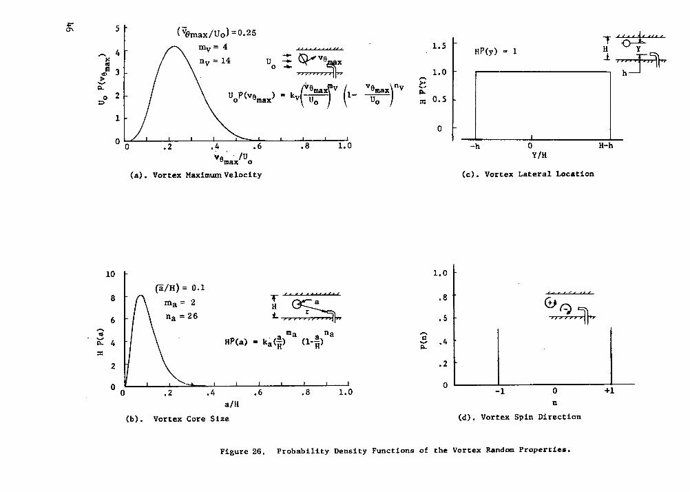
(Equation 41), and appropriate probability density functions into Equation 42.This substitution is accomplished in Appendix J and the resulting integralequation is solved by numerical techniques. The particular probability densityfunctions used in this analysis are discussed in detail in Appendix K and out-lined in Figure 26.
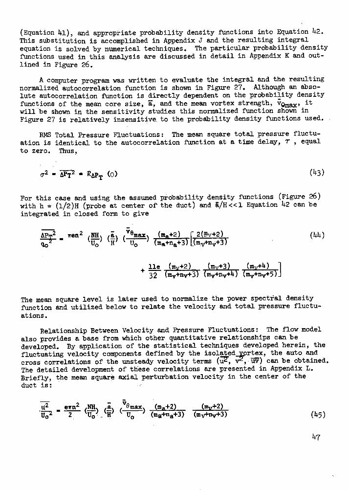
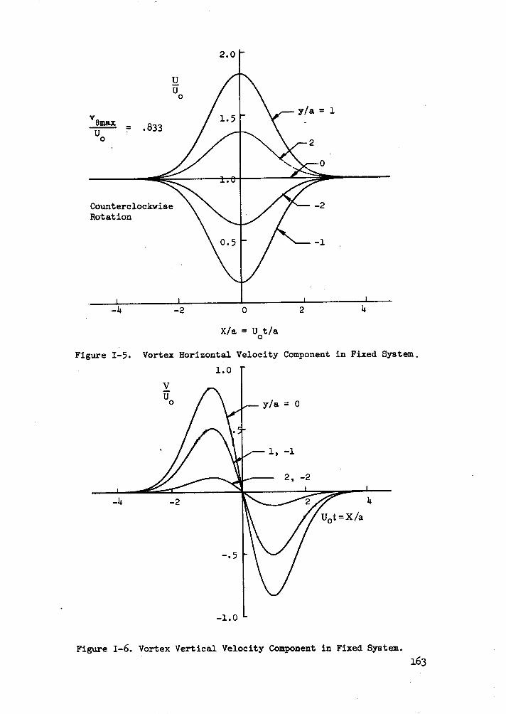
A computer program was written to evaluate the integral and the resultingnormalized autocorrelation function is shown in Figure 27. Although an abso-lute autocorrelation function is directly dependent on the probability densityfunctions of the mean core size, a, and the mean vortex strength, VQmax, itwill be shown in the sensitivity studies this normalized function shown inFigure 27 is relatively insensitive to the probability density functions used.
RMS Total Pressure Fluctuations: The mean square total pressure fluctu-ation is identical to the autocorrelation function at a time delay, T , equalto zero. Thus,
(2 A-PT2 " RAPT (0) (43)
For this case and using the assumed probability density functions (Figure 26)with h = (1/2)H (probe at center of the duct) and &/H<<l Equation 42 can beintegrated in closed form to give
The mean square level is later used to normalize the power spectral densityfunction and utilized below to relate the velocity and total pressure fluctu-ations.
Relationship Between Velocity and Pressure Fluctuations: The flow modelalso provides a base from which other quantitative relationships can bedeveloped. By application of the statistical techniques developed herein, thefluctuating velocity components defined by the isolatedyvortex, the auto andcross correlations of the unsteady velocity terms (up vZ ,-uv) can be obtained.The detailed development of these correlations are presented in Appendix L.Briefly, the mean square axial perturbation velocity in the center of theduct is:
U2 ewn2 NH Va (mA+2) (my+2)vUO U2o? ( U (ma+na+3) (mV+nv+ 3 ) (45)
47
1.0
0.9---
NOTE: The probability density functionsare given in Figure 26.
0.8
t 0.7
0. 0.6
0.5
o 0.4
N
0.3
z
0.2
0.1
0 1.0 2.0 3.0 4.0 5,0 6.0
NORMALIZED TIME DELAY -T Uo / a
Figure 27. Autocorrelation Function Computed From TheTurbulent Flow Model.
48
?.0
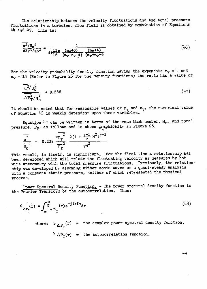
The relationship between the velocity fluctuations and the total pressurefluctuations in a turbulent flow field is obtained by combination of Equations44 and 45. This is:
u2/U 2 1APT/q 2 411e (mv+3) (mv+4) (46)
16 (mv+nv+4) (mv+nv+5
For the velocity probability density function having the exponents mv = 4 andnv = 14 (Refer to Figure 26 for the density functions) the ratio has a value of
2 = 0.238 (47)
APT/qo
It should be noted that for reasonable values of m. and nv, the numerical valueof Equation 46 is weakly dependent upon these variables.
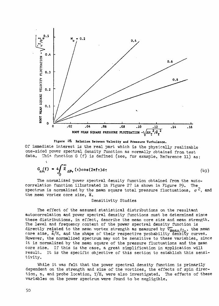
Equation 47 can be written in terms of the mean Mach number, Mo, and totalpressure, PT, as follows and is shown graphically in Figure 28.
Y
2 APT2 2(1 + Y-1 M2 )y-1ApT 2(1 2
= 0.238 2 2U0 2 2 yM2U P YM
This result, in itself, is significant. For the first time a relationship hasbeen developed which will relate the fluctuating velocity as measured by hotwire anemometry with the total pressure fluctuations. Previously, the relation-ship was developed by assuming either sonic waves or a quasi-steady analysiswith a constant static pressure, neither of which represented the physicalprocess.
Power Spectral Density Function. - The power spectral density function isthe Fourier Transform of the autocorrelation. Thus:
S (f) R (T)e-j 2 fTdT (48)
where: S AP(f) = the complex power spectral density function,
R APT(7) = the autocorrelation function.
49
o H M 10.2'C4~~ 0.4
0.40
I-.u O.S~~~~~~~~~~~~~~~~~~~~.
0.3
0
0.2
0.I1
0
0 I I /I I/
0 .02 .04 .06 .08 .10 .12 .14 .16
ROOT MEAN SQUARE PRESSURE FLUCTUATION - PT 2/P 2
Figure 2& Relation Between Velocity and Pressure Turbulence.
Of immediate interest is the real part which is the physically realizableone-sided power spectral density function as normally obtained from testdata. This function G (f) is defined (see, for example, Reference 11) as:
Gu4f) - 4 RAt ()Cos(2wfT)dT (49)
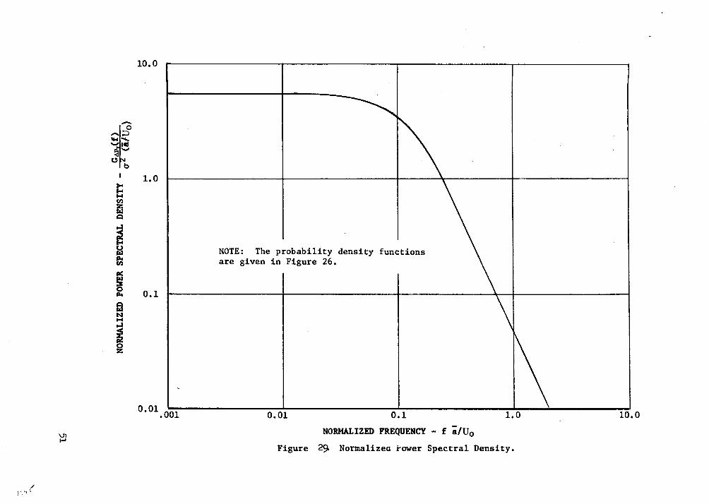
The normalized power spectral density function obtained from the auto-correlation function illustrated in Figure 27 is shown in Figure 29. Thespectrum is normalized by the mean square total pressure fluctuations, a 2, andthe mean vortex core size, a.
Sensitivity Studies
The effect of the assumed statistical distributions on the resultantautocorrelation and power spectral density functions must be determined since
these distributions, in effect, describe the mean core size and mean strength.The level and frequency content of the power spectral density function isdirectly related to the mean vortex strength as measured by vmax/u , the meancore size, a/H, and the shape of their respective probability density curves.However, the normalized spectrum may not be sensitive to these variables, sinceit is normalized by the mean square of the pressure fluctuations and the meancore size. If this is the case, a great simplification in application willresult. It is the specific objective of this section to establish this sensi-tivity.
While it was felt that the power spectral density function is primarilydependent on the strength and size of the vortices, the effects of spin direc-tion, n, and probe location, Y/H, were also investigated. The effects of thesevariables on the power spectrum were found to be negligible.
50
O
4=U
I~ 0
0~
~~
~~
~~
~~
I'A
44 N
"4=
0 a
o 0 0
0 PW
60~~~~
r4,
O C,,
0 ~
~ ~
~
0
4)
.- 0
insmaa im
ozas
mdaaIW
0(~)~VO
~ ~
1 -
0.,IN(
Y~
~dS
~/O
IZ
q"O
E-~
~~
~~
~0
~-4
r~
1-4
0
0F
p0l
(O,) -A
IS~
V~
adS o3~
iIIHO
51
0o4
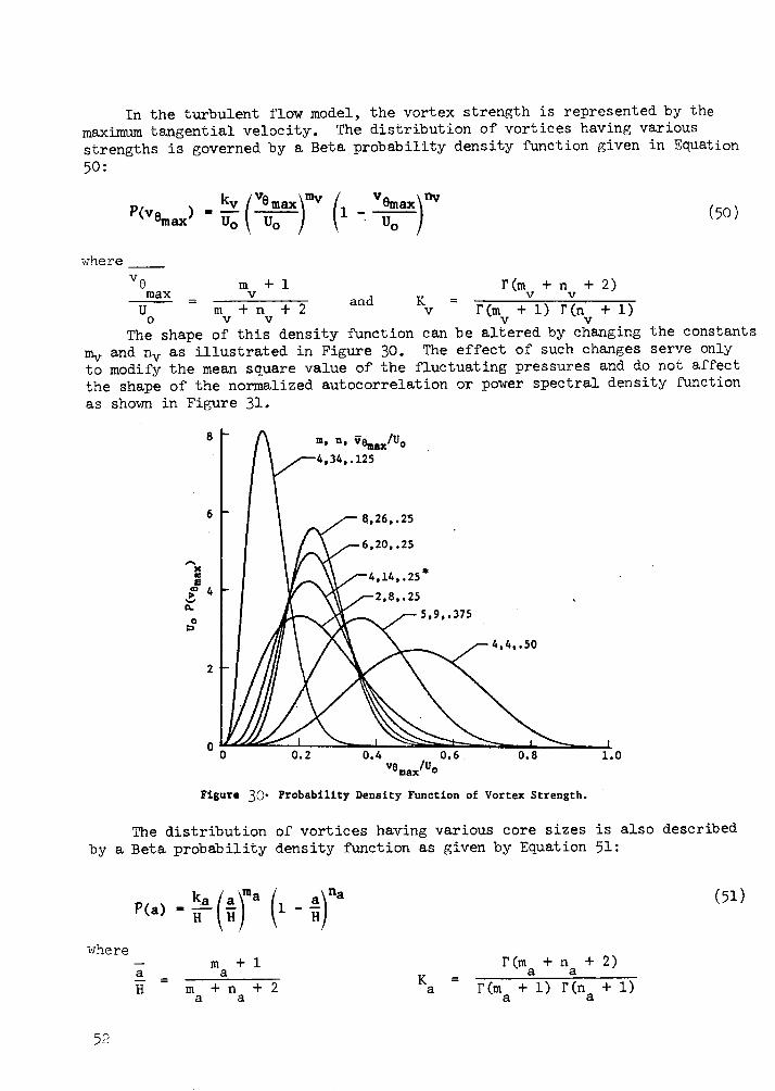
In the turbulent flow model, the vortex strength is represented by the
maximum tangential velocity. The distribution of vortices having various
strengths is governed by a Beta probability density function given in Equation
50:
P(vmkax) U, mv~vex~ U0 U0 / (1 Uo )
where
ve m + 1 r(m + n + 2)max v v vU m +2 and v r (m + 1) r (n + 1)0 V V
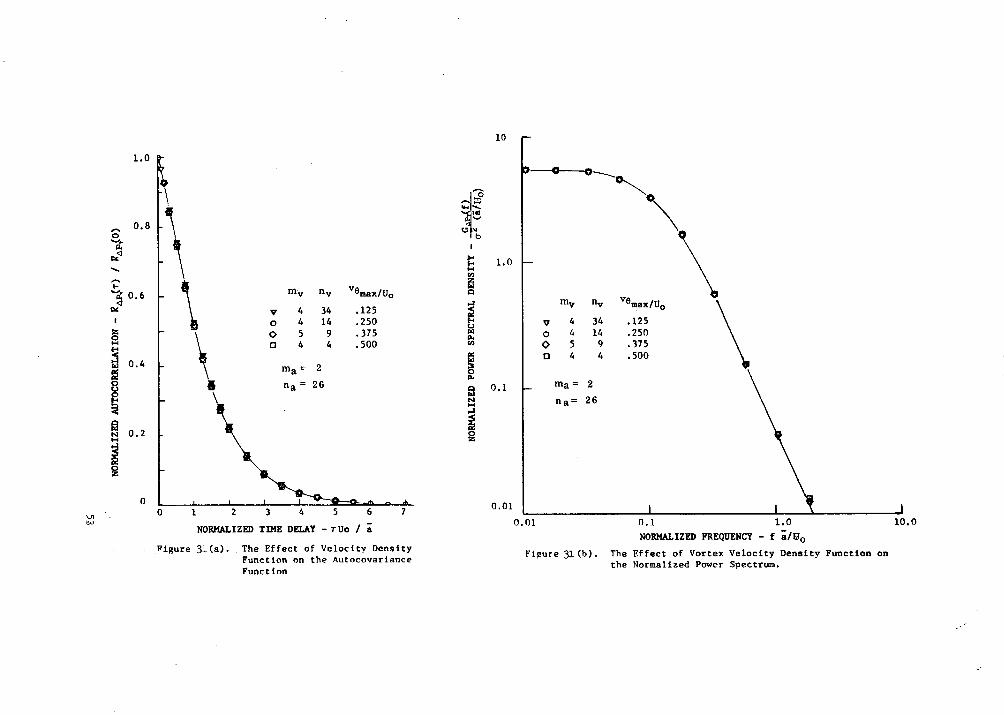
The shape of this density function can be altered by changing the constants
mv and nv as illustrated in Figure 30. The effect of such changes serve only
to modify the mean square value of the fluctuating pressures and do not affect
the shape of the normalized autocorrelation or power spectral density function
as shown in Figure 31.
8 - : am, n, veax/U o
4,34,.125
6,20.\25
4 ~2,8,.25" 9,.375
4,4,.50
VSmax/VO
Figure 30- Probability Density Function of Vortex Strength.
The distribution of vortices having various core sizes is also described
by a Beta probability density function as given by Equation 51:
P(a) k ()a ( Ha)na (51
where- m +1
a aH m +n +2
a a
r(ma + n + 2)Ka a r(ma + 1) r(na + 1)
52
(50)
-o
o
(j-)d -
-A
IISN
aa
IV
L'D
adS
3LO
da 'aZ
IIVH
ION
0x I
o 04 0
c ....
ID
V !
1 L
> ES
S
00C11
II 11
Cd C
dE
ed
Do 0O
0o
ID
( 0o) /
() a_
(0)td
v~
/ (4
dvdj
-
c0
o0
0
NO
IlrImflO
DO
lW
Cf Z
I V"IO
N
0
>8
:
0r. o0
_ G
i
o r.
1.Si'4o.ino
N
u _
0u04
0e t
U..L
" cJ
p 00
._
0 40
O
N
004
G4)004
4,- 4) I"a
1:
eAt
0o9I go
-44441E0'PkaN
,Pc 0
C;
O-4
.u
c
0 U
o -
?.-
co
u
CZ u
D- 00
N_
0 -C14-4
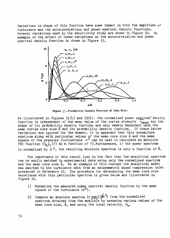
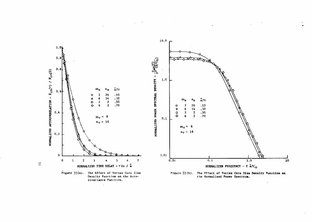
Variations in shape of this function have some impact on both the amplitude ofturbulence and the autocorrelations and power spectral density functions.Several variations used in the sensitivity study are shown in Figure 32. Anexample of the effect of these variations on the autocorrelation and powerspectral density function is shown in Figure 33.
12 m, n, a/H
4,44,.1
3,35,.1
2,26, .1*
/-6 14..32r! \ \! / lO,10 10 .5
0.2 0.4 0.6 0;.8 1.(
a/H
Figure 3 ..Probability Density Function of Core Size.
As illustrated in Figures 31(b) and 33(b), the normalized power spectral'densityfunction is independent of the mean value of the vortex strength vomax and theshape of its probability density function and only weakly dependent upon themean vortex core size a and its probability density function. If these lattervariations are ignored for the moment, it is apparent that this normalizedspectrum along with particular values of the mean core size a and the meansquare of the pressure fluctuations C 2 can be used to calculate an absolutePSD function (Gi~T(f) as a function of f).Furthermore, if the power spectrum
is normalized by a 2, the resulting absolute spectrum is only a function of a.
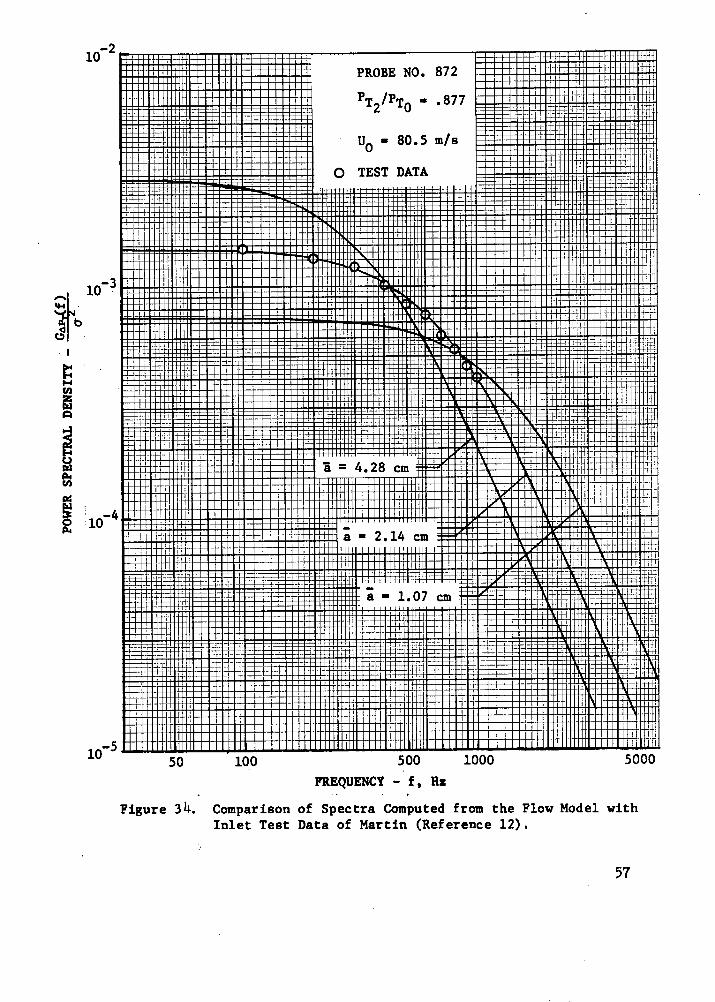
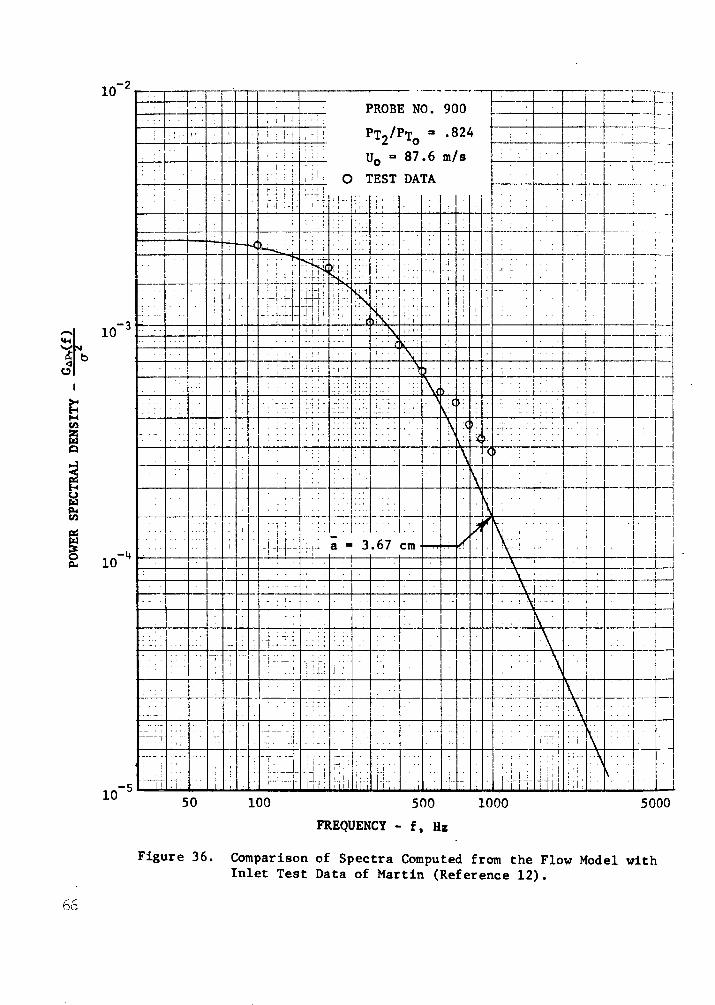
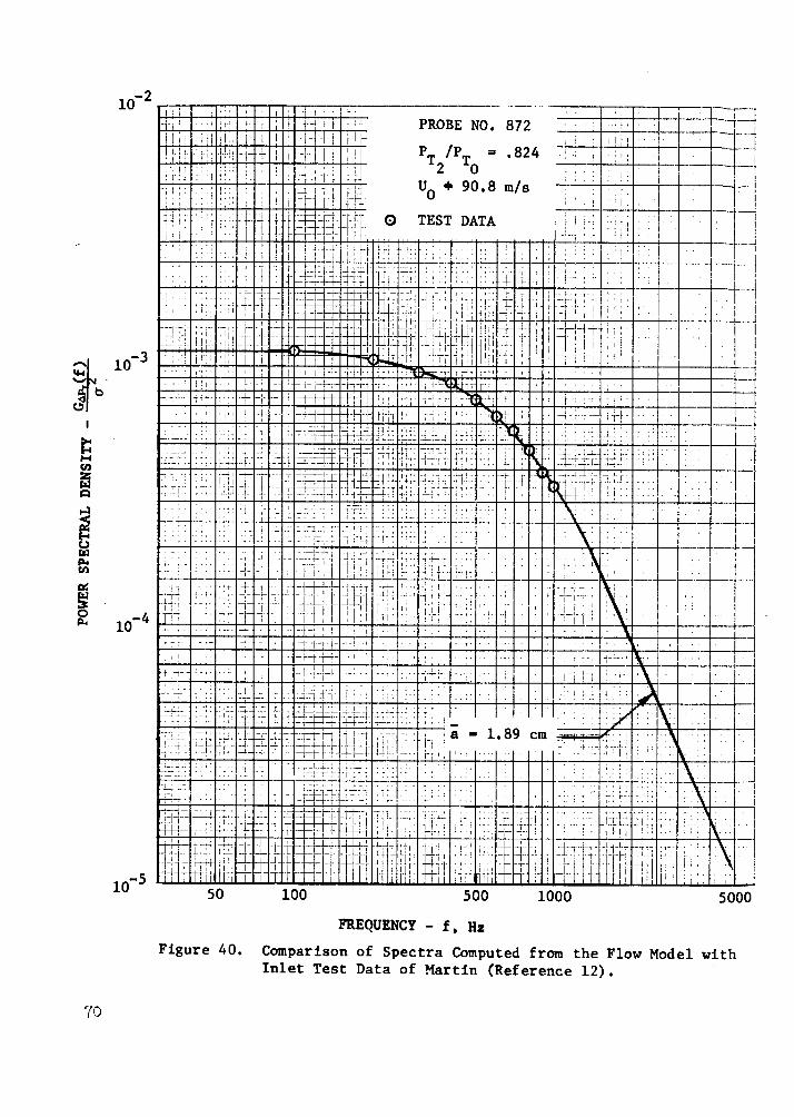
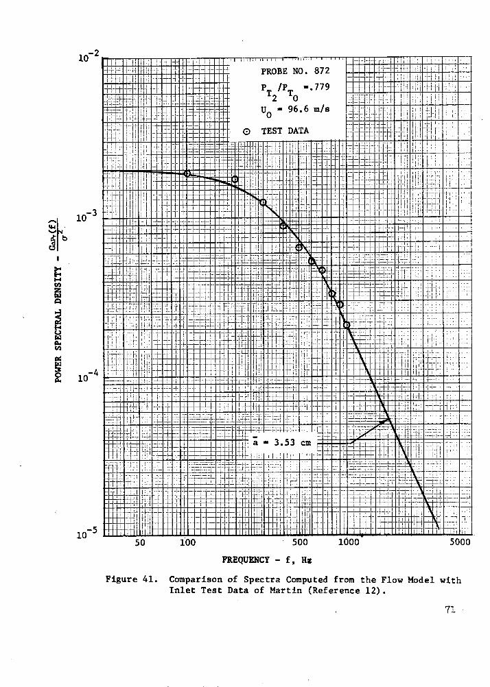
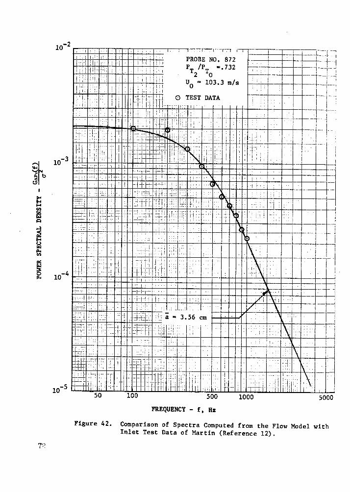
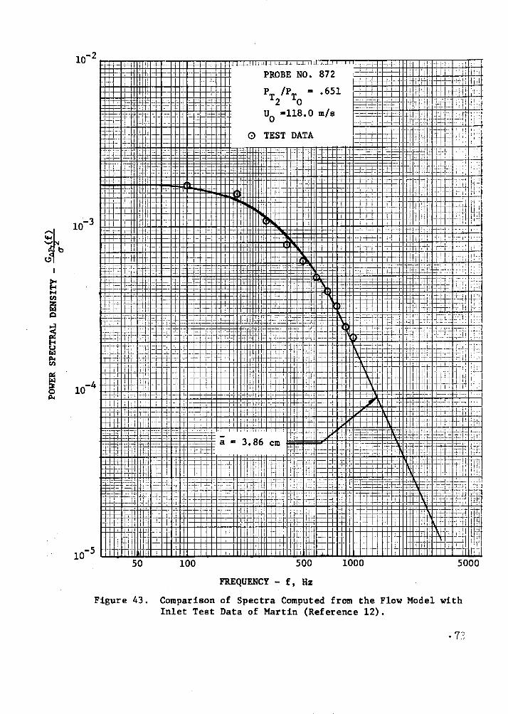
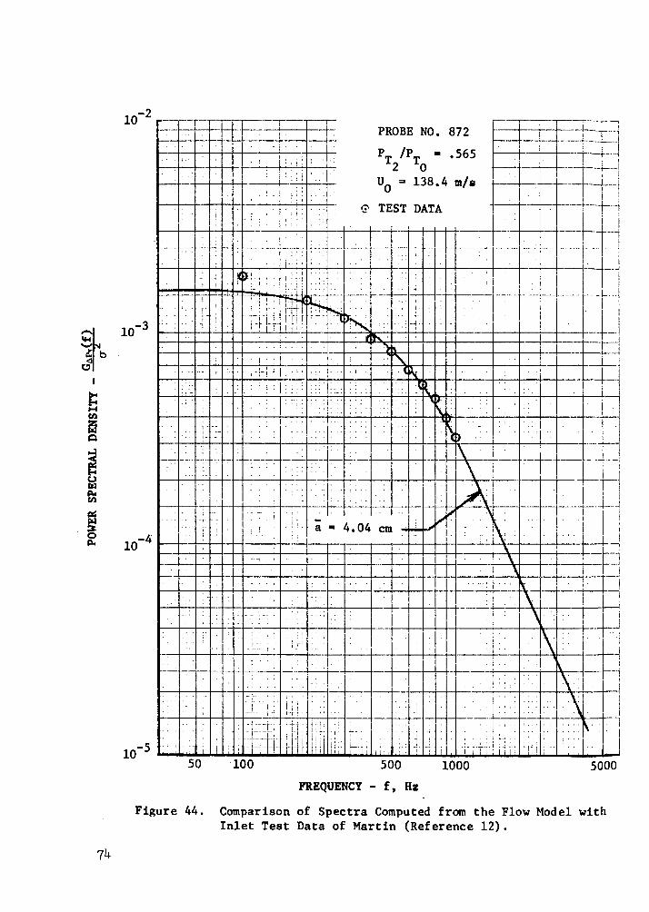
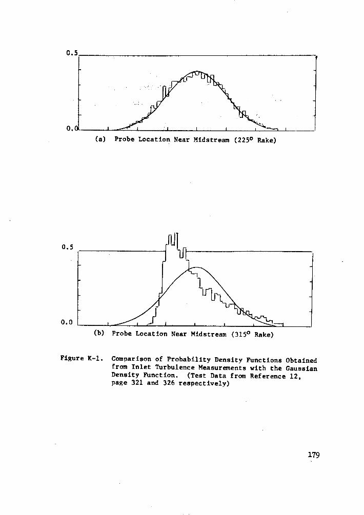
The importance of this result lies in the fact that the analytical spectrumcan be easily matched to experimental data using only the normalized spectrumand the mean core size a. As an example of this concept the analytical modelwas matched to the turbulence data from an axisymmetric mixed compression inletpresented in Reference 12. The procedure for determining the mean core sizeassociated with this particular spectrum is given below and illustrated inFigure 34.
1) Normalize the measured power spectral density function by the meansquare of the turbulence (a2 ).
2) Compute an absolute spectra (G -(f/ 2) from the normalizedspectrum obtained from the analysis by assuming various values of themean core size, a, and using the local velocity, U
o.
54
0I1
o
lc14
/ A
l
o o _o
I C
2: O
N
O
O
N
C
_ O
NG
IoL
N
°
u
0
(otdv (
-N
OL
O
ool
aZ
IO
o
¢ IIS
N-(
,Ifi-a.
I- .
(0
)dV /
\NL
(4
d
-k
IWIiW
u~
l aaziv
wio
55
0o,
_.
3) Compare the computed spectra with that obtained experimentally. Themean core size producing the best fit with the data corresponds thecharacteristic mean core size for the particular flow conditions.
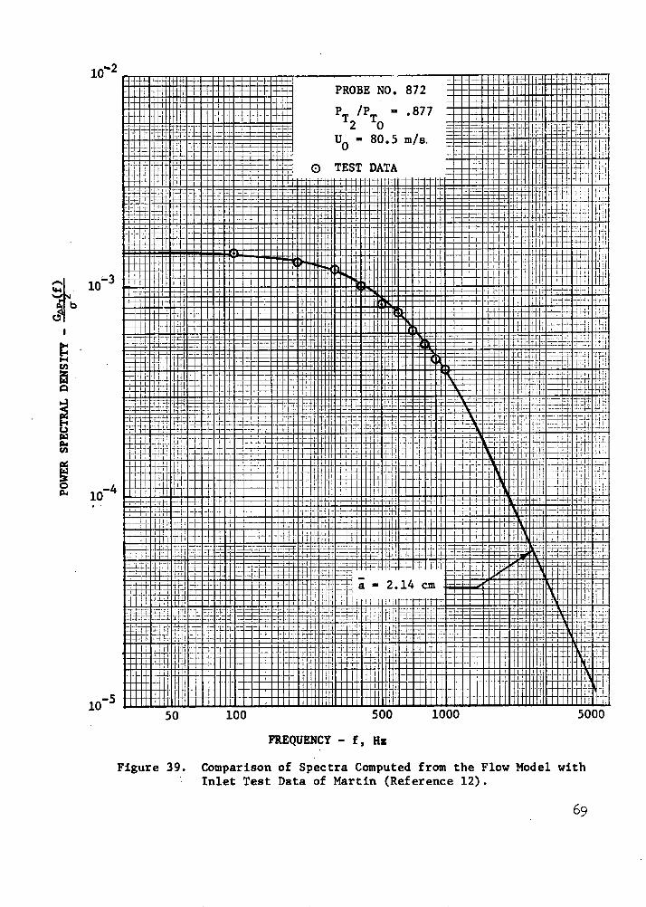
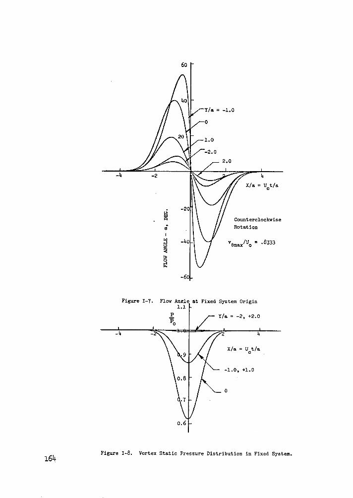
As shown in Figure 34, the mean vortex core size producing the best fit underthe constraints of both the shape of the spectrum and the area under the spec-trum ( 2 ) is 2.1 centimeters. The comparison shown yields excellent agree-ment. Additional examples of test/analysis comparison will be discussed in the"Data/Analysis Comparison" section.
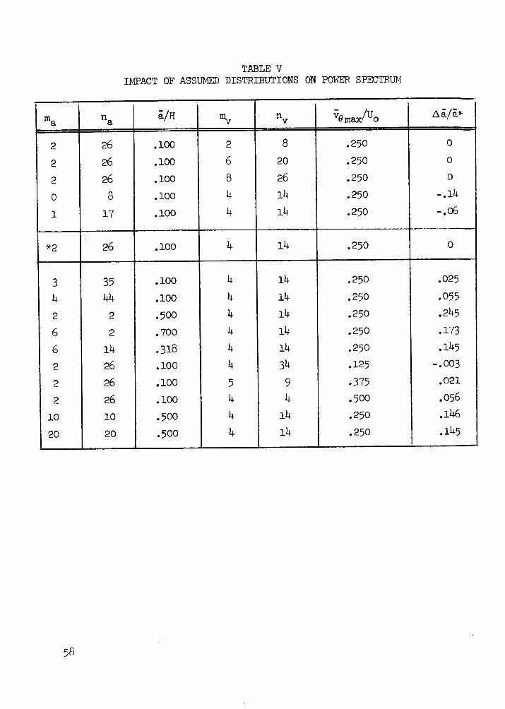
As previously indicated and illustrated in Figure 33(b) the mean core sizeand shape of its probability density function have a small effect on the normal-ized power spectral density function. Therefore, depending upon the particularspectrum used, this frequency shift in the normalized spectrum will result invariations in the mean core size, a, obtained from the analytical model when itis matched to experimental data. As a measure of the sensitivity of the com-puted mean core size to the assumed probability density function, the computa-tions summarized in Table V were made. It was assumed that the test data wasrepresented by the normalized power spectrum with the core size and maximumvelocity probability density functions corresponding to ma = 2, na = 26, andmv = 4, n
v= 14, respectively. This result is indicated by the asterisk in
Table V and shown in Figure 32. The frequency shift of the other normalizedspectra, caused by other assumed density functions, will thus cause a falseindication in actual mean core size. This error is given in Table V as Aa/a*.As shown the maximum error is 25% and occurs for assumed probability densityfunctions yielding large values of a/H. For data indicating mean core sizesgreater than 30% it may be necessary to choose coefficients that give consist-ent values of core size. This would require iteration. However, it is feltthat typical values of core size will be less than 30%, in which case the errorwill be small and hence iterations will not be necessary.
Results of this sensitivity study indicate that for turbulent flow witha/H < 0.30 the probability density functions of core size and maximum velocityhave only small impact on the overall turbulent flow model itself. This isimportant to the use of the model eliminating two degrees of freedom that mightordinarily have to be taken into account.
56
PROBE NO. 872
PT2/PTO - .877
UO - 80.5 m/s
O TEST DATA
-310
%4
I = 4.28 cm
a - 2.14 cm .11111 I I I11 II IIIIII
a - 1.07 cm
50 100 500 1000
Figure 34.
FREQUENCY - f, Hz
Comparison of Spectra Computed from the Flow Model withInlet Test Data of Martin (Reference 12).
57
I
a
ptIn
W;
-410
10-5 !5000
TABLE VASSUMED DISTRIBUTIONS ON POMER SPECTRUMIMPACT OF
ma "na i mv nv N max/Uo a I/i
2 26 .100 2 8 .250 0
2 26 .100 6 20 .250 0
2 26 .100 8 26 .250 00 I I.0 u .10O ' 4 .250 -. 14
1 17 .100 4 14 .250 -.06
*2 26 .100 4 14 .250 0
3 35 .100 4 14 .250 .025
4 44 .100 4 14 .250 .055
2 2 .500 4 14 .250 .245
6 2 .700 4 14 .250 .173
6 14 .318 4 14 .250 .145
2 26 .100 4 34 .125 -. 003
2 26 .100 5 9 .375 .021
2 26 .100 4 4 .500 .056
10 10 .500 4 14 .250 .146
20 20 .500 4 14 .250 .145
58
Scaling Law For Turbulent Flow
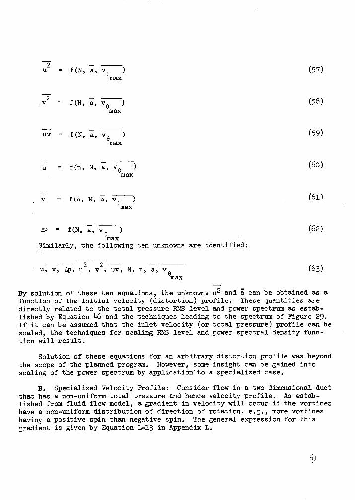
Inlet development universally begins with subscale testing. These testresults are then extrapolated to full scale to establish the expected inletperformance. The technique to scale turbulence has, however, not yet beendefined, although dimensional analyses suggest that the power spectrum willshift in frequency in inverse proportion to the actual scale size.
The scaling techniques have not been defined because of the complex natureof random, unsteady flow. "Ever since the derivation of the momentum equation,the fundamental problem of the analysis of turbulent flow has been that ofclosing the system of governing equations. This is caused by the fact thateven in its simplest form the turbulent flow momentum equation contains a"Reynolds stress" term made up of a correlation of the fluctuating componentsof the turbulent velocity field which acts as an apparent stress. Since themomentum equation is the governing equation for the mean velocity field, thepresence of this apparent stress term introduces additional unknowns into theproblem, and any equation derived without further assumptions to characterizethese unknown quantities will in turn introduce other unknown quantities. Onemethod of closing the system of equations is to formulate models for the tur-bulent shear stress in terms of already known (or knowable) quantities"(Reference 20). This formulation of models has classically been handled in oneof two ways--either some model can be postulated for the turbulent shear stressitself, or, in analogy to a laminar flow, the turbulent shear stress can beassumed to be given by some effective viscosity multiplied by a local velocitygradient.
An attempt to develop a third, perhaps more fundamental model, was madeby use of the fluid dynamic model of turbulent flow developed in this program.The model was used to define the "Reynolds stresses" in terms of the meanturbulent flow properties, providing a third model for the shear stress.
This development is outlined in Part A below. The resultant set ofEquations could not, however, be solved for an arbitrary inlet flow profilewithin the scope of the planned effort. Nonetheless, a specialized case isgiven in Part B which may give some indication of the method of scaling theturbulence power spectrum.
A. General Development: The longitudinal velocity is assumed to bedominant in the following development and the flow velocity and static pressureis defined in terms of a fixed value plus the perturbation value as indicatedbelow:
U = U0
+ u
V = O+v (52)
P = P + AP
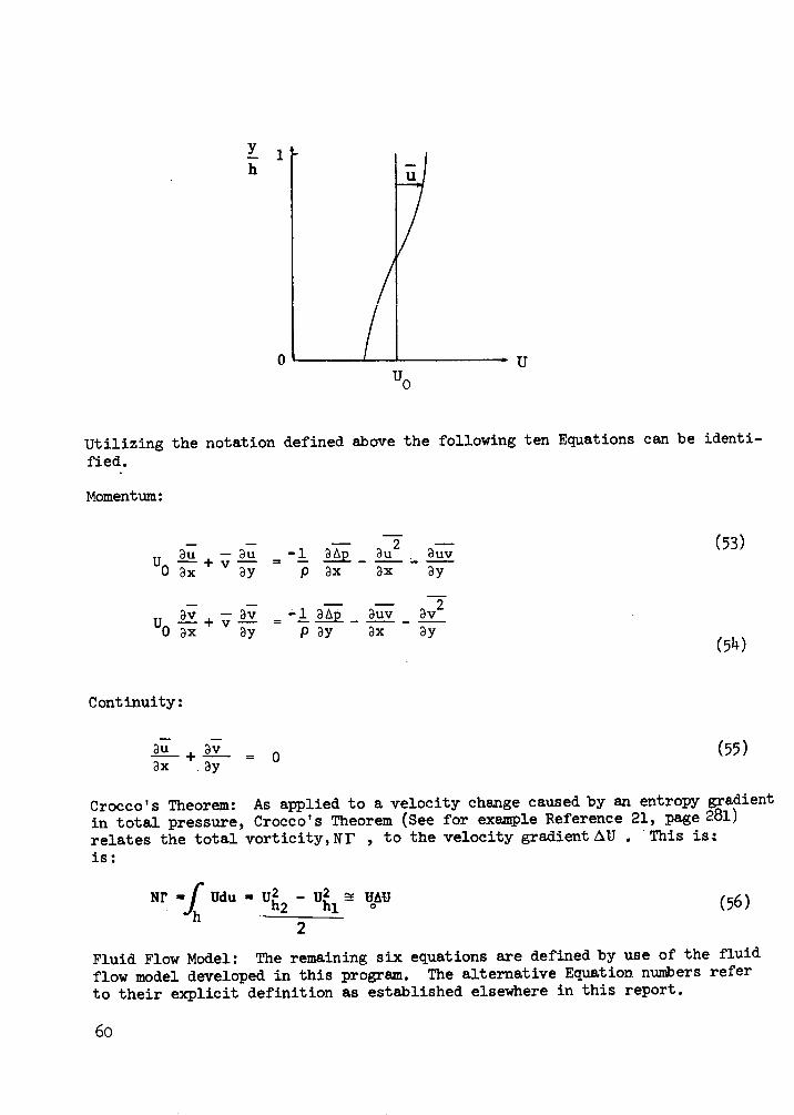
The initial velocity distribution in the x-direction serves as a boundarycondition. This distribution is shown sketched below:
59
Yh
1
0' I I
Uo
Utilizing the notation defined above the followingfied.
U
ten Equations can be identi-
Momentum:
au + u = -1 ap auo ax ay p ax ax
(53)auvay
av - av - vu av+ v = -la __ avO ax ay p ay ax ay
(54)
Continuity:
au_ + av 0 (55)ax ay
Crocco's Theorem: As applied to a velocity change caused by an entropy gradientin total pressure, Crocco's Theorem (See for example Reference 21, page 281)relates the total vorticity, Nr , to the velocity gradient AU . This is:is:
Nr -a Udu- 2 Uhi xj
2
Fluid Flow Model: The remaining six equations are defined by use of the fluidflow model developed in this program. The alternative Equation numbers referto their explicit definition as established elsewhere in this report.
6o
(56)
2u = f(N, a, v0 (57)
max
V = f(N, a, Ve ) (58)max
uv = f(N, a, v ) (59)max
u = f(n, N, a, v0 ) (60)max
v = f(n, N, a, ve
) (61)max
AP = f(N, a, v ) (62)max
Similarly, the following ten unknowns are identified:
2 2U, v, Ap, u , v , uv, N, n, a, v0 (63)
max
By solution of these ten equations, the unknowns u2 and a can be obtained as afunction of the initial velocity (distortion) profile. These quantities aredirectly related to the total pressure RMS level and power spectrum as estab-lished by Equation 46 and the techniques leading to the spectrum of Figure 29.If it can be assumed that the inlet velocity (or total pressure) profile can bescaled, the techniques for scaling RMS level and power spectral density func-tion will result.
Solution of these equations for an arbitrary distortion profile was beyondthe scope of the planned program. However, some insight can be gained intoscaling of the power spectrum by application to a specialized case.
B. Specialized Velocity Profile: Consider flow in a two dimensional ductthat has a non-uniform total pressure and hence velocity profile. As estab-lished from fluid flow model, a gradient in velocity will occur if the vorticeshave a non-uniform distribution of direction of rotation, e.g., more vorticeshaving a positive spin than negative spin. The general expression for thisgradient is given by Equation L-13 in Appendix L.
2 21 h 2 1 H-h
u-= n(.UNH 1/2 (mv +1) 41 1 2(
U 0
0(m +n + 2) [ )
L-13m +2 na a
[a a H
Equation L-13 can be integrated in closed form at the duct walls, h = 0 andh = H, by assuming a/H<<l. This results in
v 6 -2U NH ()1/2 max a (6)
U|-n (NH) (2,rre) ( ) ()(64)
h=H
v2e --2
u NH 1/2 max aU| n (U. (2Te) U
2() (65)
h=0
This will enable the maximum difference in velocity across the duct tobe established. The total vorticity flux is dependent only on this differ-ence and hence for the purposes of this example it is not nexessary to obtainthe velocity profile between h = O and H, which would require numerical inte-gration of Equation L-13. However, it is for this special case of interestthat the scaling technique will be defined which is valid only for the velocityprofile implied in Equation L-13.
The absolute value of vorticity passing between h = O and H can be com-puted by use of the flow model as in Appendix H. This flux of vorticitybecomes:
V e
Nr = n 8r NH Uo e- 1/2 ) ( max (66)' U
0
However, this flux is related to the change in velocity across the duct byCrocco's Theorem, Equation 56, which in turn is obtained by combining Equations64, 65, and 66. By so doing it is found that a/H is a constant (within theconfines of the velocity profile described by Equation L-13).
Since the power spectral density function is directly related to themean vortex core size, this result specifies that increasing inlet size wouldshift the spectrum in inverse proportion to the inlet scale. This result wouldverify the present practice of scaling the frequency content of the turbulencepower spectrum inversely with the inlet scale size. Again, this applies onlyto the specialized case.
6 2
Data/Analysis Comparison
The power spectral density functions of turbulent flow computed from thisturbulent flow model were compared with data obtained from Reference 12 for atest of a .55 meter diameter, Mach 3 mixed compression axisymmetric inlet. Thecomparisons were performed to illustrate the technique of determining the meanturbulence scale size, verify the assumptions incorporated in the turbulentflow model, and to gain insight into production of turbulence by interpretationof test data through use of the model.
The experimentally determined power spectra used in the comparisons areshown in Figures 35 and 38. The mean core size of the turbulent flow was com-puted for these spectra by assuming a mean core size and comparing the testdata with results of the turbulent flow model. These comparisons are shownin Figures 36 and 37 and Figures 39 through 44. Excellent agreement isobtained indicating the turbulent flow model accurately represents the realcase and that the flow can be modeled by the assumption of random vortices withthe indicated mean core size.
Data from probe number 900 (Figure 36), which is in the inlet duct exten-sion, approximately 3-1/2 diameters downstream of the inlet diffuser exit(Figure 36) shows some disagreement with the analysis at the higher frequencies.However, if it is assumed that this scatter is created by turbulence from twoseparate sources each having a different mean core size, a composite spectrumcan be constructed incorporating the two different mean core sizes. This com-posite spectrum is shown compared with data in Figure 45. Excellent agreementis obtained. This not only adds credence to the turbulent flow model but allowsconcrete interpretation of the power spectra. For example, it can be postulatedthat the source of the turbulence having the scale size of approximatelya = 2.0 cm. at the compressor face probe 872 may be produced by shock boundarylayer interaction. This turbulence carries through to the inlet duct extension(probe 900) but is reduced in size to approximately a = 0.8 cm., as indicatedin the composite of Figure 45. However, a new source is identified by intro-ducing of turbulence having the scale size of 2.9 cm. which may be attributedto the wakes generated by the centerbody support struts.
As a second, perhaps more significant example, consider the data of Figure39 (Probe 872) in which case the total pressure recovery was 88% and the meancore size of the turbulent flow 2.14 cm. As the inlet is operated at increasedsupercritical margins (increased terminal shock strength) the power spectrumchanges as shown by the data in Figure 44 for a recovery of 57%. -A compositespectrum for this supercritical case was computed from the turbulent flow modeland is shown in Figure 46. It indicates the flow is composed of eddies havinga mean core size of 1.9 cm plus additional turbulence having a mean core sizeof 5.0 cm. This may be indicating large scale separation is occurring and theturbulence is not only increasing in strength but in size as well.
Comparison between the power spectrum as established from the analyticalmodel and that obtained from test data shows exceptional agreement givingconsiderable credence to the development outlined herein. With this model thetotal pressure power spectrum and root mean square level of the total pressure
63
fluctuations take on considerable significance. It is specifically thestrength and size of these low pressure regions, derived by application of themodel, that are important in the inlet flow/engine interactions.
64
I I
o O
OO
--4
-4C
aa ~
CD
Dx
:
-- 0-~
p~v
0
I I
IU
0
Q
CJ
A
I tL
CC
I C
Co
0II
ID~
~~
~~
65
PROBE NO. 900
PT2/PTo =
U0 = 87.6
0 TEST DATA
i:: i: 1
.824
m/s
I '--= ..... ~f' I ~~~~~~~~~~~~~~~~~~~~~~~~~~~~~~i. -,----- 1---.L--
-- --- 1--4- - _
t ijii..
- -. 01 t- _ r_ . . . 4.I ; . . .=;·- =-. _
_~~~~__ _~*~ . - A -. - 1--1_I--
.... ,. -Ii
-- I . I
__-7 _ -- -7-- - -- ____- ---4-i- ---- *I---
._ - S -- -I-H- ----- 3.71 - ~--i-'I rI t i -I- - 4- i l -l= 1 : , t--------
Figure 44. Comparison of Spectra Computed from the Flow Model withInlet Test Data of Martin (Reference 12).
74
Ab
I
U
r.3
la
i
II! ,-r-; ! ! , I .- ,i I . : I 1
*1
10
H . I i It i iIH I i I4!
4:11.
PROBE NO. 900
PT2/PT 824
Uo S 87.6 m/s
- TEST DATA- ' im !-1 il I i_ _ i i i i _ ]i/
-Id- iiF,! i-H-!ii I ! !: , : ._ .:
! I i, i i
I ,,1 Ii~~~~~~~~~~~~~~~~~~~~~~~ 1 i I I II II II ..
i;~q:N,, ~,l!;i I-!-[~-~ -COMPOSITE·I !- "' ,ti
iii ii,, , J i , !
~~~~~~~~~~~~~~~~~~~~~~~~~~I - I +i I !-I
+L~~~~~~~~~~~~~~~~~~~~:L
i i-H -H 1-1d- M fl f I11 H hk ii ; I-I '~~~~~~~d i +Ji ++ I-H _ _
-': -":- :-
COMO4_f; ii'
-i i +i q 7~~~~~i ,~ i
i-I i I--i-i i- i I !I1 1 H4 I - I i Ar
-- i I-H i I· I i ii~~~~~~i i f :-I ii A -It
iii: ii I "~~~~~~~~~~R-Ir
~~· I ~~~~~~E~~~i !Ir_ F1'~~~~N
I 1 4+i .
W. l
50II
100.
Lrl I I i {I imf f I .tt500
FREQUENCY - f, Hz
1000dA
Figure 45. Construction of the Composite Spectrum and Comparisonwith Data from Probe 900 (Downstream)
75
-210
4b
iIEA
iN
10-3
10-4
5000
Ll.Li11
i
1-
I
I
i It
L.II i-
-111-f-4 --dS-tri I
E. -L
Im rTI iil
I I t t ill . .. ,iid~:'t: J I i. i I n i, F MJl-l~'
50 100
.lD- .. . _ .i--I 7-
t7I. ' ': ';1
., }.- ;+
500 1000
: : -7 . . . . - , I-1 . . , . . .-TI ... ..
i , T:41: -.LIIHq
5000
FREQUENCY - f, Hz
Figure 46. Construction of the Composite Spectrum and Comparisonwith Data from Probe 872 (Diffuser Exit) at Low Recovery
10-3
10 - 4
~b
!
lM
UPaad
En
10-5
76
] ,' 1; ' ~ '
CONCLUSIONS AND RECOMMENDATIONS
The analytical developments reported herein provide a fundamental approachto the problem of inlet/engine compatibility. With further development, thisapproach will provide a method of evaluating inlet tests and engine designsearly in the propulsion system development cycle. Ultimately, it shows promiseas a method for predicting and evaluating the effects of distortion and turbu-lence on engine stall characteristics, prior to system test.
The following are the more significant conclusions arising from the workto date and suggestions for continued activity to achieve the basic programgoal: establishing the fundamental relationship between inlet distortion andturbulence and loss in compressor stall margin.
Conclusions
(1) The effect of circumferential total pressure distortion on the lossin compressor stall margin has been established analytically. The analysis hasshown that the stall margin loss is directly a function of the distortionpattern, the distortion level ((Pt - Ptmin)/ t), and of the compressor rotorreduced frequency, k =wc/2 U.
(2) The rotor'chord is the principal design variable in the reducedfrequency, k, and therefore emerges as a significant engine parameter indesign for compatibility.
(3) Favorable comparison of distortion and engine stall data with analysisresults is considered verification of the fundamental hypothesis of theanalysis. Specifically, a circumferential total pressure distortion will resultin an unsteady flow over the rotor blades requiring these unsteady aerodynamiceffects to be included in the stage characteristics.
(4) The accuracy of the stall prediction technique is sufficient tojustify the simplified approach which considers an overall compressor workbalance rather than a detailed stage-by-stage development.
(5) A phenomenological model of turbulent flow typical of that found inaircraft inlets has been developed by combining statistical techniques withthe basic laws governing fluid dynamics. The power spectral density functionand root mean square level of the fluctuating total pressure take on consider-able significance as a consequence of the model resulting in a means ofdetermining the strength and extent of time variant low pressure regions.
(6) Favorable comparison of spectra obtained from the analytical modelwith test data of a Mach 3 mixed compression inlet verify the Turbulent FlowModel.
(7) The agreement with test data for both the Compressor Analysis andTurbulent Flow Model strongly suggest that compatibility problems, heretoforeonly attacked by empirical methods, are amenable to analysis.
77
Recommendations
(1) Both the Compressor Analysis and Turbulent Flow Model are considereddeveloped to the point necessary to initiate the program to achieve the longterm goal of establishing a fundamental relationship between both inlet dis-tortion and turbulence and compressor stall margin loss.
(2) Further comparisons of the compressor analysis with test data arerecommended for refining the method. The data used should provide the detaileddistortion patterns, compressor geometry and compressor operating conditions.
(3) Additional analysis of turbulence data from a well documented inlettest program should be conducted to demonstrate the use of the turbulent flowmodel in isolating the source of turbulence and establishing turbulence decaycharacteristics.
(4) Finally, the developed relationships between distortion, turbulenceand loss in compressor stall margin should be compared with data from anaircraft flight test program to verify the analysis.
78
APPENDIX A
Analysis of Unsteady Potential Flow on an Airfoil
This appendix contains a detailed discussion of the physical mechanismseffecting the interaction between an airfoil and the surrounding unsteady flow.The effects of unsteady airflow or airflow motion on an airfoil below thestalling angle of attack are explained in terms of the physical mechanism inpart A and then related quantitatively with the governing mathematical rela-tionships in part B.
A. The Governing Physical Mechanisms. - Lift on an airfoil is a conse-quence of the unequal pressures acting on the upper and lower surfaces. Inpotential flow these pressures along the surface of an airfoil can be computedfrom the velocity field by use of the equations of motion. The result of apotential flow solution, with zero circulation, about a flat plate of length,'c", and inclined to the stream at an angle,d ,would yield stream lines similarto those sketched in Figure Al.
Figure Al: Potential Streamlines Around anAirfoil with no Circulation
The required boundary condition is that of zero flow through the plate. Thisis equivalent to the plate being a streamline which by definition implies zerocross flow. The lift on the airfoil is given by Equation A-1 and is designatedas the non-circulatory lift, LNC. Although the lift component is zero forsteady flow, it can be non-zero under non-steady conditions.
C
LNC - o (PU - PL) dx (A-l)
To bring this mathematical model into agreement with experience it isnecessary to move the rear stagnation point aft to the airfoil trailing edge(Kutta condition). This can be accomplished by imposing a circulatory flowaround the airfoil as shown in Figure A2.
79
F
a+~~~~~~
NON-CIRCULATORY FLOW PURE CIRCULATORY FLOW COMBINED FLOW
Figure A-2. Flow About an Airfoil with Circulation.
By so doing an equal circulation of opposite sign is shed from the airfoil suchthat the sum of the two is zero. The circulation about the airfoil imparts anadditional velocity field around the airfoil and must be accounted for inobtaining the total lift. This additional lift is directly proportional to theamount of circulation r required to move the stagnation point aft to thetrailing edge and is given by Equation A-2.
LC - pur (A-2)
This in turn is related to the angle of attack, a, of the airfoil by
1 2LC ' pUor - 2a(r(pU
o2 )c
wherer - nUoca
(A-3)
(A-4)
Total lift is therefore composed of two terms each caused by imposing a boundarycondition:
L - LNC + LC (A-5)
where C is of non-circulatory (potential) origin and is a consequenceof the requirement for zero flow through the plate
and LC results from the circulation required (Kutta condition) to movethe rear stagnation point to the trailing edge.
In steady flow and as indicated by the symmetry of Figure A-1, the liftdue to non-circulatory flow is zero. Thus, in steady flow the total lift isapproximated by the circulatory term,
L - LC ' (~pU2)c 2wa (A-6)
80
For unsteady airfoil motion, however, inertial forces due to the finitemass of fluid that is forced to adjust cause the non-circulatory lift to benon-zero. As an example, consider the resultant lift due to oscillatoryvertical translation and pitching motion (about the mid chord) of an airfoil:
C2LNC - fP W [y + Uc] (A-7)
where wp , is termed the virtual mass per unit span associated with thevertical acceleration y and/or U(. It is equivalent to the mass of a cylinderof fluid with a diameter equal to the airfoil chord.
In addition, for any change in motion of the airfoil a trailing edgevortex must be shed to force the stagnation point to remain at the trailingedge. This adjustment requires a finite time and it too contributes to theresultant airfoil lift. The vortex shed is non-recoverable and might beconsidered as a dissipative or damping force. For the case mentioned abovethe lift of circulatory origin is:
LC - ipUcC(k) [j + Ua + c a ] (A-8)
Combining equations A-7 and A-8 the total lift for an airfoil undergoingoscillations in the vertical direction and along the pitch axis is as follows
*L - ffp S + U&]I + rpUcC(k)[y + & + ] (A-9)
For a general treatment of non-steady airfoil/airflow refer to References18 and 19.
B. The Governing Equations. - The pressure forces due to unsteady flowacting on the isolated airflow discussed in Part A will be quantitativelydescribed below. This will be important in developing the effects of unsteadyflow on the stalling airfoil lift coefficients in subsequent sections.
Airfoil lift in unsteady airflow is dependent upon three prime factors:
1. The type of motion occurring. This can be classified by thefollowing:
(ii) Airfoil undergoing horizontal translation(iii) Airfoil exhibiting pitch oscillation
(b) Free stream airflow unsteady - airfoil steady(i) Airflow with vertical gust(ii) Airflow with horizontal gust
2. The type of input, e.g., sinusoidal, step, arbitrary, etc.
3. The times associated with the disturbance compared with the airfoil"time constant".
Unsteady lift equations for the various classes of motions are summarized inTable A-1.
81
gI 4'
111
_ H
'IN
.ou50I=1
oi
HLt
0 H-61
C~lI
~o .4 44
a4 44
OBU I
O
I I
°
_t
_
4.4
4' 44
-4'o
44
~
4 to
W 0
44
to04
4m04101
04.
1:
e 0 V
e. Z0
lk .
II
(d
0 0
t> 0
>' 0
'd+
ES
E~
~~
~~
~
,R>0
7o o
3 * ,a,l 4 -.4100
a0o
0
.,4,
iIT
K
0
>4a
*to
'te
*8
0)
0 ..a,
C10
o
0H
.4.
0
.In
a AtoVI
c ea
0 O
0)00)I;.. a0 0
R O
.
A' a:
4-0
40c
iriPII
00)
I at;
U.
I
p a
e0
;a4
:4>-I,!,VUell
N0.0]I0)0
82
clo
Pl
M.e~-
.e-
0-iV%I,V
o
As indicated by the response functions in Table A-1, the change in liftcharacteristics is delayed in response to instantaneous change in airfoil angleof attack or flow velocity. The two physical mechanisms causing delay arefound to be:
1. inertia of the mass of air requiring adjustment and
2. the finite time for the trailing edge vortices to be shed and causeadjustment with the flow field leading to a damping of the unsteadi-ness.
These phenomena are analogous to a damped mass/spring system which can bedescribed by a second order differential equation, such as:
m dz + d + c2x - f(t) (A-10)
where: m = mass
c1= damping factor
c2= spring constant
An unsteady flow field about an airfoil will most likely be composed of acombination of several of the above motions. Nevertheless, each of the abovemotions can be approximated by a second order differential equation and thecomposite flow field modeled by a general second order equation. This responseof the airfoil to these motions in unstalled flow will form the basis uponwhich to develop the phenomenological model of an isolated airfoil subjectedto angle of attack excursions beyond the steady state stall limit, and ulti-mately to represent the phenomenological model in usable, mathematical terms.
83
APPENDIX B
Solution of the Differential Equation for theEffective Angle of Attack
The effective angle is related to the instantaneous angle of attackthrough a second order linear differential equation. The differential equationis solved below for step, ramp, and sinusoidal changes in the instantaneousangle of attack. LaPlace transform techniques are utilized in the solutions.
In terms of dimensional time, t, and dimensional time constants, t1 and t2the governing equation is
d (aff
dt
- a) + (L +t d (at 2 eff
1- a0) + tt 2 (aeff - a)
1l 2
1(a - a )
t 1 t 2 inst 0
It is convenient to non-dimensionalize this equation by the airfoil velocity,U , and chord c. A non-dimensional time and time constants are defined below:
T = tU/c
T1 = t 1 U/
2= t2U/c
Employing these definitions Equation B-1 becomes:
d2
2 (aeffd-r
- ac) + (1 -- d (e ff1 2
- Ca) + T (aeff aO)12 ffa
1rl
2(r inst
- a)
This is identical to Equation 2 in the main text. Equation B-2 is a linearsecond order differential equation, is conveniently solved by LaPlace Trans-form techniques and is represented in the LaPlace domain as:
L (aeff - a )
L (ainst - ao) (1lS+ l) (T 2
where T (s) = transfer function
and s = LaPlace dummy variable
84
(B-2)
The effective angle of attack can be obtained for simple changes in theinstantaneous angle of attack, ainst - a o, by the method outlined below:
aeff - =eff o L -1 {L(a ff- a)} L -1{ (ainst - ao) x T(s)}
For example, assume that the instantaneous angle of attack, a inst,increases as a step function of time as shown in Figure B-l.
L (ainst - ao)
aeff - ao
1
- 1= + 1 s (s T1 + 1) (S T2 + 1)
aeff - oa - ainst o
11+ 1 [ -e
-T/T
T -T [Te 1-2 1
] (B-5)2 ~~~~~~~(B-5)
The effective angle lags the instantaneous angle as shown below.
a
1.0
0.5
I
u 02.0 4.0
DIINKSIONLZSS TDM, t - tU/c
Figure - Iesponae of EffectiLe Angle of Attack to a Step'Chanse
The actual shape of the a eff curve will depend on the system time constants,VI and r 2 , as indicated in (B-5).
As another example the effective angle is found for a ramp input in a inst,with a ramp rate of increase, dca = constant = c1 .
dt
85
(B-4)
L (ainst - ao)
C1aeff ao =L1
eff - o
s2(ST1 + 1) (sT2
2
c1 z2
- Z1
+ 1)
21 -T/T
e I+T- - 2z2 - T1 2
An arbitrary variation in the instantaneous angle of attack can be repre-sented by a Fourier Series as discussed in the section "Extension toArbitrary Variations in Angle of Attack." A Fourier series utilizes the sum ofsine and/or cosine waves to approximate the variation. Solution of the differ-ential equation (Equation B-2) for a sine wave will therefore allow solutionfor arbitrary instantaneous angles of attack. This solution follows:
ainst ao = Aainstsin(wt)
sL (a it C a) = 2 2
-1 -a
ef o- a = (ST1+ 1) (ST2 + 1) (s +d )
a -aeff o
A ainst
2k
1I2
e-T/T1+
-T/T2
12 )(2+ 4k2)
+
2k 4k2 ( 1
sin (2kT - %)
+T 2 )+ ( T2 J .
1T2 4k )
Tl (B-6)
}
where k = (o/2
86
(B-7)
= Cl/S2
1
( 2-1) ( 2 + 4 2) (IT1
+
The exponential decaying terms are neglected for periodic motion, simplifyingthe amplitude of the sine wave results in
sin (2kT - ~)
(1 + 4k T12) (1 + 4k T22)
The amplitude of the sine wave is notedFigure B2. The phase shift is
m = tan- 1 (2k) + tan-1
(2kT2)
= f(k) sin (2kT --) (B-8)
as f(k) for convenience and shown in
(B-9)
-. 10 1.0
Reduced Frequency, k -cwc/2U
Figure B2. f(k) vs Reduced Frequency for Several Values of T2.
87
eff o
A in st
1.00o
v
I
0
I
44
.5
0.01
Preceding page blank jAPPENDIX C
Increase in Airfoil Maximum Lift Coefficient forUnsteady Flow Test Data
A limited literature survey of the effect of unsteady flow on the maximumlift coefficient of an airfoil was conducted to establish an estimate of thetime constants associated with airfoil stall in unsteady flow.
Available data were for a ramp rate of increase in angle of attack definedas an increase in angle of attack at a rate = d ca /dt = constant. The liftcoefficient achieved at stall with this type of unsteady motion was found tobe greater than that achieved with steady flow. This increase, A CLmax, isshown in Figure C-1 as compiled from several sources.
Solution to the governing differential equation, Equation 2, for the ramprate of increase was given in Appendix B. The analysis is dependent on the non-dimensional time constants r1 and r2. Based on a comparison between compressorcomponent data and the analysis it was established that by setting the two timeconstants equal, 7 1 = T 2, the best match between data and analysis could beachieved. For this reason, analytical results are shown compared with thedata in Figure C-1 for values of ~1 = T2 = r= 2.0 and 3.5. The comparisonindicates time constants on the order of 3c/u are representative of theinteraction between the unsteady flow and stall.
PRECEDING PAGE BLANK NOT FILMED
89
-4
cA
'A(AII(4
'4\9
oe
C
-co'I
>
,
er-r)
C
1
'. · ·
I I
e 4CU
e ~ 10~
ts
' ee
A Iaa
,2 .GE
a
c0 ..0
Trswls
oV lS
dN
I
C0I
D=
)ffmO
D
MM
T
1IM
ul~
to l
0IIU2
0coI
0
0co02
40cH 0
4U,
C)
o0
E-i Q0
4,C12
H
C
.0:
4
90
0
0
APPENDIX D
Relating Inlet Distortion to Rotor Blade Lift Coefficient
The objective of this Appendix is to develop the relationship between thechange in rotor blade lift coefficient required to perform the increased com-pressor work and the inlet distortion. Since a multistage compressor is builtof individual stages having similar characteristics, the effect of a change inmaximum angle of attack of one stage will therefore be similar to the responseof the next stage and derivatives or influence factors should be similar. Theprocedure will be to equate the change in work (due to distortion) done on theairflow to the change in work done by the rotor blade. From this equality willcome the relationship between CL and pressure ratio which can be evaluated interms of the operating point and the total pressure distortion.
Change of Work Done on the Air. - The compressor work per unit time doneon the airflow is:
AE = w Ah pA UAh (D-l)a x
where Wa = airflow = PAxU
A h = ideal compressor total enthalpy increase
(A E) = increase in energy of the air per unit time.
Ax = flow area normal to the axial direction
U = axial velocity
Consistent with the parallel compressor model which is based on a uniformcompressor exit pressure, inlet total pressure distortion will require a changein work done on the air to maintain this uniform exit pressure. The change inwork can be written:
· ' dA
(D-2)AEI P Ax U AhAE J x
This change of work done on the air must be balanced by the change inwork done by the rotor.
Change of Work Done by the Rotor. - The rotor work is as follows:
ERTR = 2 PvR ARTRURTRCL (D-3)ERTR 2 R ARTRURTRCL
91
where ERTR
= work per unit time done by the rotor
VR = air velocity relative to the rotor
ARTR
= rotor area = chord X unit span
URTR = compressor blade velocity
CL = rotor lift coefficient
The useful work done on the air by the rotor will be somewhat less dueto the finite efficiency. Thus:
ER = nER
(D-4)
ER=1 PV22 PVR ARTRURTRCLn
The change in useful rotor work required by distortion is therefore:
d(ER)
.EER
dp + 2dVR
P VR
dARTR
ARTR
dU+RTRURTR
dCL dnCL nL
(D-5)
Equating the Change in Work. - Since the useful work done by the rotormust be equal to the work done on the air equations (D-2) and (D-5) can beequated:
dp dAx dU +dAh d 2d R+ A + Ah +p A U Ah P VR
dARTR
ARTR
dURTR+ U
RTR
dCL dnC nrlL
Since the rotor area, the axial flow area, and speed remain constant, andassuming the change in efficiency due to distortion is strictly a secondaryeffect and therefore negligible, the equality reduces to the following:
dU dAh 2dVR dCL (D-6)U+ dAh' +V C- -~=h VR L
It remains to find a relationship between dCL, dU, and dVR.
established from the typical stage velocity diagram.This can be
92
Velocity Diagram. - In the compressor mid stages, the stage stator exitangle will be to a first order independent of distortion around the circum-ference. Making this assumption the velocity into the following rotor will beas below:
\ \ \ \ \ Stage n-l stator row
Stage n rotor cascade
r = a + 8. = constant
tan B = tan (r - a) = U/URTR
.'. U = U tan (F - c)
Taking the derivative of U
dU = -URTR (1 + tan2 (r - a)) da
and
dU ( -a a tan (r - a) da_U (\tan (r - a) 1 ) a
Similarly:
VR U (cos (r - a))-1R RTR
= URTR ( cos (r - a) -2 sin (r - a))da
dVR = - a tan (r - a) daV aR
(D-7)
dVR
(D-8)
93
Recall:
CL
= 2 a
and
dCL da
CL a
Using these relationships equation (D-6) becomes:
[tan ( - - a tan (r - a)t an (T - et ) 1J
da dAh+ dAh =a Ah
- 2 atan (r - a) d +a a
Combining terms:
d [ - adec C tan (F - c) + a tan (Fa n r 0 - a)J-1 + dAh
Ah'0
Typical flow angles (r - aattack of 12 degrees.
) are 35 degrees (Reference 13) and angle of
tan 350 = .7
a = 120 = .21 radians
d[ .15- l =dAhAh
In essence
dU dVdU 2 R 2U VR
dAh - daAh a
dCL
CL(D-9)
The additional required work comes from(or lift coefficient). This additionaldistortion.
an increase in blade angle of attackwork must be related to the inlet flow
Compressor Work and Inlet Distortion. - The average work done by thecompressor on the airflow remains constant. However, that section of thecompressor operating in the region of low inlet total pressure must increasethe pressure ratio to pump the flow to the uniform compressor exit pressure.It is assumed that this additional work is divided evenly among the compressorstages and the stage work, " A (A hi)," can be related to the required increase
94
in overall pressure ratio as shown below:
Ah. = C(T - TT P Ti Ti-1
ith- stage work
TTi = total temperature atcompressor stage
the exit of the it h
I I I TTi_-l = total temperature at the in:
stage(exit of ((i - l)th) stage)
let to the iu- '
The c]
dahi CpdTTi
Ahi
Cp (TTi - TTi_1 )ha!nge in overall work is t
nz d(Ah.)
d(Ah) i=1Ah n
i Ahii=l
Since dAhi dC
Ahi CL
therefore given by Equation D-ll.n d(Ahi) Ah
Ah.i=l .
n
i=lAh
Equation (D-ll) becomes:
n dCL Ah.
C nd(Ah) i=1 CL n Ahi dCL/C LAh n n Ah.
E Ah 1i=l i
therefore
d Ah dCL
Ah overall L stage
where Ahi =1
(D-10)
and
(D-11)
and
(D-12)
(D-13)
95
I
Thus it is shown that the overall increase in compressor work is relateddirectly to the increase in airfoil lift coefficient of a single typical stage.By assuming this additional required work is divided evenly among the com-pressor stages the required increased work can be equated to the requiredincreased pressure ratio as developed below. The overall compressor work,assuming an efficiency of 1Oo, is given by:
TT3
Ah = C (TT- TT2) C T (-- 1)
[(P T 2
CTT
Taking the derivative the following results
d (Ah), 1d~nh~dRP CP ·T2 ( Y- ) P -1 (D-14)
dR CTT ~dRTherefore
d(ah) ( dR (D-15)h ry-1 R
1 -(R ) Y P
where Rp = overall compressor pressure ratio = PT3/PT2
By combining equation (D-13) with this result the relationship between theincreased pressure ratio and required blade lift coefficient is derived.
dC r-1 dRdCL dAh Y p (D-16)
CL Ah y-l R1 -R y
Realizing that the increased pressure ratio required of the compressor isthe negative of the change in inlet total pressure, (distortion)
dR dPT2-- T (D-17)
T2
equation (D-16) produces the relationship between the stage lift coefficient(dCL) and the distortion (dPT
2) as given by Equation D-18.
96
da dCL
a CL
y-1Y
1 - R (l-y)/yP
dPT
T 2
22(D-18)
This result is combined with the effects of unsteady flow on the stallinglift coefficient to establish the effect of distortion on the compressor stallmargin.
97
preceding pae blankAPPENDIX E
Computation of the Loss in Compressor Stall Margin
Computer Program Description
I. ABSTRACT
A computer program has been written to calculate the loss in compressorstall margin due to inlet steady-state circumferential total pressure dis-tortion. The program is written in Fortran IV and is operational on the LTVACCDC 3300 computer. The mechanics of the program are discussed below, and aprogram listing included. Input instructions and examples of the input andoutput are given.
The program input is the circumferential totalcan be of arbitrary shape. A Fourier Series is thenthe coefficients are modified by a transfer functionin dynamic airfoil stall of the rotors. The loss inthen calculated as an output.
pressure profile whichfit to this profile andto account for the delaystall pressure ratio is
II. FORMULATION
A. Mathematical Description
1. Distortion Amplitude
The distortion amplitude is defined from the input total pressurefield as the difference between the average and the minimum pressure dividedby the average pressure (Pt - Ptmin)/Pt. The distortion amplitude is used tonormalize the calculated loss in stall margin.
2. Fourier Series
arbitraryindicated
The technique of predicting stall pressure ratio loss fordistortion profiles utilizes Fourier series fit of the profile asbelow.
PT(e) = a + En=1
00
a cos (nO) + E b sin (ne)n nn=l(E-1)
PRECEDING PAGE BLANK NOT FILMEDI
99
where
Pt(8) = total pressure as a function of circumferential position,
n = harmonic numberTr
= 1a PT P,()de
an = -PT(8)- cos (nO) de (E-2)- Tr rr
1bn I P T() sin (nO) dO
-Tr
The Fourier series can also be represented by sine terms. Thiswill facilitate calculation of the loss in stall margin as will be shown later.
Let
a = c sin (4n) Cnan
bn = cn cos (pn) an
c = a + b bnn n n
-1= tan (an/bn )n nfl
Then
a cos (nO) + bn sin (nO) = c sin (ne + 4n)
The series is thus written as
PT(9) 0 cT = 1 E- _ -n sin (nO + 4n)
PT n=l PT (E-3)
where the minus sign is the result of a change in the limits ofintegration from, -7-to Tr , to 0 to 2 T.
100
3. Compressor Loss in Stall Pressure Ratio for Arbitrary DistortionProfiles
The technique to establish the loss in compressor stall marginis fully described in the section of the main text entitled "CompressorAnalysis." Briefly, loss in stall margin is defined with the aid of the fol-lowing figure which represents the process on a steady state compressor map.
B dt w St&U La
Operat in Line
/o.lov
The "clean" stall margin is defined as
R - RPB P 0
SM = R
p0
(E-4)
101
The stall margin with distortion is defined as
R - RPE PO
SMDist = R (E-5)P 0
The loss in stall margin is thus the difference between thesetwo equations:
R - R
PE; PO (E-6)RPO
This loss in stall margin is normalized by the distortion levelas defined in Equation E7
Dist = (PT -PT )/P T(E-7)
min
resulting in a normalized loss in stall margin, Equation E-8.
ASM (E-8)
(PT PT .)/PTmin
The technique to compute this normalized loss in stall margindue to an arbitrary inlet distortion profile is briefly as follows:
(1) The input distortion profile is represented by a Fourierseries.
(2) The response of the compressor to this pattern is equalto the sum of the response to each of the components of the Fourier series.This is computed by the program.
(3) The highest compressor stall pressure ratio, during acomplete revolution of the rotor, is used to compute the loss in stall margin.
B. Program Input
1. The program is designed to compute the normalized loss in stallmargin assuming a second order response with the non-dimensional time constants,
T 1 = '2 = 3.5. This is the recommended mode of operation. In such a case
102
the only required input is the distortion pattern and the compressor reducedfrequency, k.
However, if it is desired to change the non-dimensional timeconstant and/or the "order of response" the program is designed to accept theseas input items on Card 1 (Refer to Figure E-l).
2. An arbitrary number of total pressure values are input into theprogram in order of increasing circumferential position up to a maximum of 144.The corresponding circumferential positions, which are arbitrary, are required.As an option it is possible to use the sine input subroutine to generate singleor multiple harmonic sine waves of a specified amplitude in percent. Threesample cases are given which demonstrate the use of both types of input.
Multiple cases are run by repeating all cards except the initialcard which gives the number of cases to be run.
3. The number of harmonics used in the Fourier series can be changedby changing the value of the parameter KN in the main program. KN = 72 isrecommended for complex patterns where five degree resolution is adequate. If,for example, 2 1/2 degree resolution is required, set KN equal to 144. Moreharmonics will increase the accuracy of representing the input wave at theexpense of more computing time; the effect on the calculated loss in stallmargin is usually small.
4. The input data arrangement is illustrated in Figure E-1. The dataon the first card is used to signal the number of cases to be executed duringthe run. All control parameters are input for each case. The input data forthe arbitrary distortion profile and the sine wave distortion profile are dif-ferent; and are illustrated in Figures E-l(b) and E-l(c), respectively. Adetailed description of each input parameter follows. Parameters input inI format (see Figure E-l) are right adjusted.
JJ - Number of cases to be executed during run, input only once.
NORD - Order of system response.
KREF - Compressor reduced frequency.
T 1 - First time constant; if zero input, T 1 defaults to 3.5.
T2
- Second time constant; if zero input, T2 defaults to 3.5.
LSPR - Key for long print out; LSPR f 2, long printoutLSPR = 2, short printout
KKKK - Key for sine or arbitrary distortion profileKKKK = 1, sine input followsKKKK Z 1, arbitrary input follows
K - Number of data points in arbitrary distortion profile defini-tion 1 < K < 149.
103
FORMATPARAMETER
FORMATPARAMETER
. AND SO ON THROUGH CASE "JJ".
CASE 2
CASE 1
16JJ
Figure E-l(a). General Input Data Deck Arrangement.
/ F1O.5 F10.5 F1O.5 F10.5 F10.5 FlO.5 F10.5 FlO.1T (1) T (2) T (K)
Figure E-l(b). Arbitrary Distortion Profile Input Data Deck Arrangement.
FORMATPARAMETER
Figure E-l(c). Sine Wave Distortion Profile Input Data Deck Arrangement.
104
T1
PT(I) - Total pressure distortion profile; arbitrary units, eitherratio of local to freestream or avg, or absolute dimensions(PSIA, PSFA, N/M2, etc.).
T(I) - Circumferential location (degrees) to describe distortionprofile, must be input in ascending order.
MMM - Sine wave input distortion, number of cycles per revolution.
AMPL - Sine wave distortion maximum amplitude.
5. Most of the output data are labeled. The printed data include asummary of the input data, a short or long output data format, and a printerplot of the instantaneous and effective pressure ratios.
a. AMPLITUDE - Sine wave distortion profile maximum amplitude,input parameter AMPL
b. MULTIPLE/REV NO. - Number of sine wave cycles per revolution,input parameter MMM
or
INPUT PT THETA - list of arbitrary distortion profile total pressure andangle pairs; these are PT(I) and T(I) input parameters,from I = 1 to K.
PT AVG - Average total pressure of the input distortion profile.
LOSS IN STALL MARGIN - This is the loss in stall margin.
NORMALIZED LOSS - Loss in stall margin divided by distortion, wheredistortion is (PT - PTmin)/PT.
The printer plot is composed of:
1. the input instantaneous total pressure ratios
2. and the effective total pressure ratios versus circumferential loca-tion, in degrees.
105
The long printout also includes
PT/PTAVG - linearly interpolated total pressures divided by theaverage; computed from the input profile.
THETA - Circumferential location, radians.
A(I)/AVE - Fourier coefficients, a, for harmonics 1 to 18, dividedby average total pressure.
B(I)/AVE - Fourier coefficients, b, for harmonics 1 to 18,divided by average total pressure.
C(I)/AVE - Fourier coefficients, c, for harmonics 1 to 18,divided by average total pressure.
PHI(I) - See Equation (E-3), radians
PHASE ANGLE - Transfer function phase shift for harmonics 1 to 18,radians
AMPLITUDE RATIO - Transfer function amplitude ratio for harmonics 1 to 18
PT2INST - Instantaneous total pressure computed from Fourier fit
THETA - Circumferential angle, radians
THETA - Circumferential angle, degrees
PT2 INST - Instantaneous total pressure ratio computed from Fourierfit and normalized by average total pressure.
PT2 EFF - The computed effective total pressure ratio, normalizedby the average.
SPR LOSS - The loss in stall pressure ratio.
INPUT RPI/RPO - Defined by Equation (18) in main text.
RP(EFF)/RPO - See Equation (17) and Figure 8, in main text, fordefinition.
C. Subroutine Descriptions
1. Subroutine LINR
Subroutine LINR accepts the input total pressure and angle data.The angles (and corresponding pressures) are input in increasing order and maybe unevenly spaced. The subroutine linearly interpolates the data to generatetotal pressures every five degrees (KN = 72).
106
2. Subroutine ALF
Subroutine ALF accounts for the dynamics of the rotor stall pro-cess. The subroutine accepts (1) the number of harmonics to be used, (2) theorder of the response, (3) the compressor reduced frequency, and (4) two timeconstants. The output is the phase angle and amplitude for each of the har-monics.
3. Subroutine Sine
The sine subroutine may be used to generate sinusoidal input data.When the sine subroutine is used, no pressure or angle data are input. Thesubroutine accepts the amplitude, and the number of sine waves per 360 degrees.
4. Subroutine Plot
The PLOT subroutine generates a printer plot of the interpolatedinput total pressure ratio, and the calculated effective total pressure ratio.The plot is suppressed when the output circumferential spacing is other thanfive degrees (i.e., KN d 72).
D. Program Limitation
The dimension statements allow for a maximum value of KN = 144 whichcorresponds to 36 harmonics, and 144 circumferential spaced total pressures.The plot limits are fixed; the upper limit is 1.25 and the lower limit is 0.75.If the order of response is other than two, the two input time constants haveto be equal.
107
IV PROGRAM LISTING
A listing of the main program and the four subroutines are given below:
108
1., CD
0.I A-tD.4
I-19I0'II
'- -
H
0.
im
G
LI'~
~~
~~
~~
'
(A70.
U
0-
0'II-
II1I3I-ar1x
tLI
'Ci 0B.
ftIIZ
hII
I- 0
.IIi
.&
. I° I- c) I
1el
I |5 |IF
|
a D
in
c.
0.I0
O
Li0B
.
in0A-n
UII
I
'0.
uzLII
,I-in
ih
in H t
I
Cd, ..J
C' ~
U,
u
CD 1,
-, *
'.4 Z
~
~ ~ z
2 aX
t
'.4 U
.I-o
1 1 L
1.4 0.
I-r0
anwlZ-ItLI'
II
i
<
J I'
I-B
1 H
,
II~~
~~
J Ii
-
-*- 4 EZ
, H
c
II
*~
~~
I in
C
01-
II y
x t-
9I
H
UC, I
19
IIIIII
� II1 �II
ilEL;\i .:iL~i\\~t;\\
!: ISj/ii
V ;I
4 I
t I0
_, N
oIIl C
..1-
I4
I
11
I I
)):I iI l /IIIl
1 ,i .//lll/I
I LI 11L
I-l_I- I
I -E
I I
% I
-
I z
LI iF./ It-I i, ---· ~
f rZ,~~.1-Ir4
I-a,C .
I! I
T IuI&
. VI 'Il
IH;"i l .
zlfl
l
I. I
IIII l
Il
r
I
PO
CY
~ ~
~ ~
~
.4~
~~
~~
~~
~0
0
&
-4
4 U
.
.4 .4
Ii i
I- ~ ~
~ ~
a~
~~
~~
~~
~~
~~
~~
~~
~~
~~
~~
~~
~~
~~
~~
~~
~C
a
N~
~~
~~
~~
~I-N
w
al0. u
s j Itw
II
IIII
IL~
~~
~~
~~
~~
~~
~~
~~
~~
~~
~~
~~
AI
-J 0.~
~~
~~
~~
~~
~~
~~
~~
~~
~~
~~
:I
o~
~~
~~
~
WI-
:- I
4
.
-4
I~i .
I i
i
to Fll
Ir 14
.4
F- I
l 1l 1
I I
II 1I l
I U
, i
1 hl
w
w
I, I
N
ZI
" 4
N1w
;w#4.
ww
.
(AC
--
UM
.M
%
44
a I
M0
MC
.3C
o --
0..I
I-IIIZ
ZU
%
2..J
4--4-~~~~D
~ U
M4
M
L
1 4
IL
M0
M
IZPI)D
*.
-rL
t' .42
.4It'C'.JZ
*
I-Id
.4
.4Z
~
~ ~
~ 11
.1~
~~
~~
~~
~~
~~
~~
~~
~~
~~
~~
~~
~~
~~
~~
~~
~.
-t~~
~~
~~
~~
~~
~~
~~
~~
~~
~~
~~
~~
~~
~~
~~
~~
-
00
-t~~
~~
~~
~~
~t
I- bJ~~~~~~~~~~~~~~~~~~~~V
o IJ.J4*~~~~~~~~o
0
I -,2
O.Z
-"~
~~
~~
~~
~-
IL IL
~~
~~
~~
~~
~~
~~
~~
~~
~~
~~
~~
~~
~~
~~
~~
I
V. SAMPLE PROBLEM
A. Input Data Description
'T'4~T"7n T".-g? 8 sn 1rr_75;57 U 17.. N'~B'? .17745sT l" t1Zi 40'q-7 Rq0t~ 3tttn4 9, 0 ; 6 '3t45~? 8t
.^ . : 9. 90.- _
I ._ _ _ _ _ - _2 .2 -Z .1 3,*9 IS5F- -- 10
123467 2369636 016__ _ -9 CI--T
10 9.3 o.. Zh1- T0.I21 i *n-I.
I Z ] 4 5 h r R1234567 9012345 6 78O 4-900i--T-F-q- f 567f . lc}. 1?3 4-67Tq012345A7R9? 01234567B90 1 346 7890
B. Output Description
Pages 120 through 125 present the long output for the arbitrary distortion profileinput. A two per revolution sine wave short output is presented on page 126. Afinal short output for a complex distortion profile input is presented on page 127.
Solutions of the Navier Stokes Equations for Vortex Flow
Definition of several vortex flow fields are developed below by solutionof the Navier-Stokes Equations for both a steady and for a time dependent vor-tex. The choice of a vortex for use in describing turbulent flow will be madeand the boundary conditions leading to this choice discussed.
Navier Stokes Equations of Motion:ten shown below ¥
Using the cylindrical coordinate sys-
V1*
CYLINDRICAL COORDINATE SYSTEM
the equations of Motion of an incompressible viscous fluid in twoare:
av, + r ar + vr e r ar + a $ + r ayr + 1 a2'at 3r r a6 r 3r 3 r ar pa
__ aVa VA are 1 ad Va2v 1 a 2at r ar r ae r Fr P a +j ar r+ rr -r (-ae
Continuity:
ar (rVr) + av_ 0i-r ae
dimensions
- 2 avQ - Vr)
(F-l)
+ 2 avvr - V)ae ae )
(F-2)
(F-3)
For the vortex model, Fe and Fr are zero and the pressure P and velocitiesvr and ve are independent of 8. Further assume that no source or sink occurs
PRECEDING PAGE BLANK NOT FILMED 129
within the area enclosing the vortex, in which case vr - 0. Equation (F-2)then reduces to the following:
ave W V 2 F 1 e vI (F-4)at r + r r r r e
Solution of the Navier Stokes Equations. - There are several solutions ofequation (F-4), each representing a different set of physical boundary condi-tions. Five of these solutions are discussed.
For a steady flow v is independent of time and equation (F-4) reduces tothe following:
a21 1+ r (F-5)- -- Ve o
The two solutions are:
(a) For forced vortex (solid body rotation):
ve- klr (F-6)
This is shown in Figure F-1.
(b) For a Potential (free) vortex:
ve = k2 /r (F-7)
This is shown in Figure F-2.
A combination of equations F-6 and F-7 has been used to approximate aviscous flow model. Specifically, the following form results and is shown inFigure F-3.
ve- l+r (F-8)
This satisfies the Navier-Stokes equations when r<<l or when r>>l; not, however,at r - 1 (see Figure F-4). Viscous effects cause non-recoverable losses. Theselosses dictate the vortex velocity and energy decrease with time. As a conse-quence a solution containing viscous dissipation must be time dependent and nosteady state solution that fits the boundary conditions imposed by real flowscan be found.
For unsteady flow, three basic solutions have been found. The first is asfollows:
r 2
\ v8 . - e 4vtI (F-9)veI w130
voe r
2
r
Figure F-1. Velocity Ratio of a Steady Forced Vortex
(Solid Body Rotation) --- Equation (F-6).
+1
V8
-2
131
+1
v0
-4 -2I2
v8 C
r
-1. L
Figure F-2. Velocity Ratios of a Steady Potential
Vortex --- Equation (F-7).
-6I
6r/a
132
I I 1 l
vo 2(r/a)
VOmax 1 + (r/a) 2
Figure F-3. Approximation to a Vortex Having a Forced Rotation
Near the Center and a Potential Motion at Large Radii ---
Equation (F-8).
+1
v e
V¥ max
133
V*
O max
2
(r/a)
2(r/a )
1 + (r/a)2
4r/a
-' - 2(r/a)v *0 max
Figure F-4. Comparison of the Approximation with the Two Steady Solutionsof the Navier-Stokes Equations.
134
+11
ve
V0 maxvftax*
V0
vo mOmax
-6 -4 -2 6
This represents a vortex that at zero time has a potential flow field. Att > 0, viscosity effects begin to cause the vortex to decay as shown in FigureF-5. The radius, r shown in Figure F-5 is that arbitrary radius havingthe velocity, vy, a? time equal to zero. This solution is given, for example,in Reference 14 page 81.
A second solution exists for a vortex that is started impulsively at timet - 0, having a strength concentrated within a zero radius (a Delta function).At time t - 0 the influence of this line vortex spreads. The normalized shapeof this vortex is shown in Figure F-6, and compared with the other vortex flowfields in Figure F-7. This particular solution is attributed to G. I. Taylorin Reference (15).
Its equation is given below:
r 2
ve -B I (F-10)
It will be assumed that this model most nearly represents the type of vorticesin turbulent flow where the influence of a formed vortex is at first limited butincreases radially with time. Reasons for this selection are discussed belowin Appendix G.
A set of additional solutions to the Navier-Stokes equations can be foundby the technique of separation of variables. These solutions are as follows:
-A2tv 06- · Z (u) (F-il)
where: Z(u) - Jl(u), J_l(u), YI(u), Hl(u), Hj(u)
Jl(u) - Bessel Function of the first kind of order 1
Jl(u) - Bessel Function of the first kind of order -1
Y1(u) - Bessel Function of the second kind of order 1
Hj(u) - Hankel Function of the first kind of order 1
H1(u)* - Hankel Function of the second kind of order 12U2 . (X2 r 2 )/v
These solutions however are oscillating with radius and as a result do notfit the boundary conditions of the problem at hand.
135
+2
ve
( vOer
+1
4vt/r2
O
1 2 3
r/r0
Figure F-5. Velocity Ratio for a Potential Vortex Allowed to BeginViscous Decay at Time Zero. --- Equation (F-9).
136
1 2 3r/a
V/vOmax - (/a)
Figure F-6. Velocity Ratio of a Vortex Started Impulsively at Time Zero--- Equation (F-10).
137
+1
VO/Vomaxl
+1
vo/Ve max
vA - (r/a)Vemax
-2
2(r/a)l+(r/a) 2
-1(rhro)
Figure F-7. A Comparison of the Vortex Velocity Ratio for Three FlowFields Satisfying the Three Different Boundary Conditions.
138
-6 -4
Vomax
2 4r/a
- ev8
V6r-ro
t-to
(r/ro)24vt/ro z
e - ½ [(r/a)2-1]
APPENDIX G
Boundary Conditions for Vortex Model
For the purposes of developing a fluid dynamic model of turbulent flowcertain boundary conditions must be imposed on the vortex description that meetthe physical conditions associated with the turbulent eddies. These are assumedto be as below:
(a) ve must be zero at a vortex radius of zero (viscous forces predominate).(b) ve must be zero at a vortex radius of infinity.(c) v6 must be continuous between 0 <r <-" and satisfy the equations of
motion.(d) The zone of influence of an eddy or vortex must be small at first, as
when it first forms, and grow with time; as opposed to an eddy that isfully established at all radii, then proceeds to decay, i.e. the trans-fer of momentum is outward with time.
A summary of various vortex flows is given in Table G-1 along with a graphicalrepresentation of the vortex and its respective ability to meet the boundary con-ditions. The Figure numbers in the Table refer to Appendix F. As shown, only thevortex formed by the impulsive start meets all the required boundary conditions.For this reason it was chosen as a typical vortex in turbulent flow and will beused in further development of the fluid dynamic model of turbulent flow.
A word of caution, however, the vortex proposed assumes a laminar viscos-ity coefficient. Bear in mind that any given vortex may have smaller eddiesforming in the core which in themselves may produce "turbulent" flow in whichcase decay would be governed by an eddy viscosity and occur an order of magni-tude faster. This turbulence could also cause modification of the velocityprofile. Because of the assumption to use a laminar viscosity coefficient orspecifically a viscosity coefficient independent of both radius and time, andbecause of the assumed impulse start of the vortex, the option must remain opento select other vortex velocity fields subject to experimental verification.
139
cot
mP44)40.4go
Aeea_I
X
B
.4
"ii0
oz t h
:9 0 tp
0IoI
a AU
I?S)>4So404
O
a11
6to
_I
lii
co'I0
cItoS.mA)mAs)
r-4I_
t
i1
x 4)e
· B
-
4)A
)A
..44
'A
0 p
4 g
t .
11
-C
Im
1
0
tS o
O
ay
4)
go iS
i A
c
t X
4
J4 'A
0
42HP
4 a.
Vi+
, 9+
9
O
S) w0A;
tlbR
g
1 o
C.
eIrz
moa;$4
0M;
S
IIIi
Yb0;W0t02
U0 044
4
o tn
8~
140
I
41
II
%*.1 1 11Ap11
I 0
III
n o ait
I
gI
-
iE
APPENDIX H
Details of the Selected Vortex Flow Field
A vortex flow field that satisfies the unsteady Navier-Stokes Equationsand the proper boundary conditions was selected as representative of thoseeddies typical of inlet turbulent flow. This particular solution was firstgiven by G. I. Taylor in 1918 and represents a vortex formed instantaneouslyin undisturbed flow. The influence of this impulse begins to propagate out-ward at t = 0 . Table H-1 is presented in summary giving the velocity, angularmomentum, vorticity, circulation, and static pressure distributions of thevortex along.with the rates of decay of each parameter. Derivation of thecharacteristics and graphical representations follow.
Velocity. - The vortex flow field selected for detailed study is definedbelow:
r 2
r -4vt (H-l)ve B t- e
Where: v = velocity in angular direction
B = constant
r = radius
t = time
v = kinematic viscosity = //p
The radius, a, at which the velocity is athe derivatives Ovaq 4r, equal to zero or
r2
vA B 4vt 2Br2 - 4vtar P 4'4t3
Thus:
r 2
2vt
maximum can be determined by setting
=O
1
or
.r~v/ 6Max'r@V . vYe,1 a - ,2vt (H-2)
Note that a grows at a rate proportional to, t2. Normalizing the vortex radiusby a, Equation H-1 becomes:
141
IA
If)L
i
I I
I I
•i~~~~~~~~~~~~~~~~~~~~~~~~~~~~-,4I
I I
I~~
~~
~~
~M
N
C
0
* U
~~
~~
~~
~~
~~
~~
~~
~v2
4i o~~~~~~~~l
IAJ~
~~
~~
~~
~~
[,g
:4
I~~
~~
I.
I-I
0 0
Ai
4I ,
, ~
~ ,
cll ~~~~~~~~~~~~~~~~~cll
c"
U~~~ .
C' ,
*I',,N
"
0 'I-l
Ip 2 2
.41 a~
~~
~~
~~
~~
~~
~~
~~
~~
~~
~~
.)
YI
I I.-
.
II,~~
~~
~~
~~
~~
~~
~~
~~
~~
-
0NI N
.
_] I
C~
~~
~~
~~
~~
~~
~~
~~
~~
C
N
0 04
pa ~~~~~~~~4)
I~~
~~
~~
~I
-i
04 4
8.41. 8.4
04
r
rim~
~~
I%
I
4)~
~~
~~
~~
~~
~~
~~
C
aI~
~~
~
.- 4)
>
l
o ~
~~
~~
~~
~~
~~
~~
~~
~~
~
u uh
t U>
i~~
~~
~~
~~
~~
~~
~~
~~
~~
~~
~~
~44
1 0 $ 4.
4) 0
45)4~~
~~
~~
~~
~~
~~
~~
13
142
Il
, ,r 9
v - B - e (H-3)
Normalizing v. by the maximum value, the velocity ratio is:
,r (-v -e a (H-4)
This is shown graphically (for a given time) in Figure H-1.
Vortex Angular Momentum. - The equation of moment of momentum (angularmomentum) is as follows:
Mw = (~ x r)dm (H-5)
where the arrow denotes a vector quantity, "X" a cross (vector) product, and"dm" an elemental mass. In the cylindrical coordinate system
ye
r r r
m - p x Volume
dm - prdedr (unit depth)
·where denotes-the unit vector in the e direction
r denotes the unit vector in the r direction
Therefore:
M -JfvorprdOdr r2
2 2f r e 4vt dr
To integrate let [ - r 2
dE - 2rdr
dr -/
r3 - (r2)3/2 , &3/2
143
1.0
r/a
v - r/a le -½[(r/a) -1] IV max I i
Figure H-1. Velocity Ratio of a Vortex Started Impulsively at Time Zero.
14k
Thus
B fp 4vt dv
Mw - rpB(4v)2 (H-6)
Note: The angular momentum is independent of time and hence is conserved.Because Mo is conserved it would be a logical term in which to expressthe constant "B".
Thus:
B (H-7)
Vorticity.- Vorticity is defined as:
R ' x v-
t" (rve)t
.la Br2 4vt)
r 2
- e 4vt 2B Br2 i (H-8)
At a given time the maximum vorticity is found by setting the derivativeof vorticity with respect to radius equal to zero. Thus:
.-r2 r2 r2an 2B 2r - 4t Br 4vt Br3 4vt
ar ' - -iz e -- e + 4-vZt e=
P- ~ax 2ar@Qn ' qax
rn I |IMax - (H-9)
Substitute this radius in equation (H-8) the maximum vorticity is:
2BInlMax ' tr (H-10)
The maximum vorticity therefore decays proportional to 1/t2 .
Substituting the radius at which the vorticity is maximum (Equation H-9)into the expression for vorticity (equation H-8) and using this maximum vorti-city to normalize equation (H-10), the following becomes the normalized vorticity:
145
r.2,1(2 - r2 -l)e a
)
and is shown plotted in Figure H-2.
(H-1l)
Circulation. - Vorticity is associated with a local elemental area. Thisvorticity can be different at each spatial location in the flow field. By multi-plying each elemental area by its associated vorticity and summing the resultsover the total area, the circulation r will result. Thus:
~~r -1_~ 3~ d A - P~ *.~ ds ~(H-12)
ds - rde ;
r = verde = B 2 e
rr 2 4vt
r - 2wB 7. e
r 2
4vt de
(H-13)
The circulation approaches zero at infinite radius indicating that thearea associated with negative vorticity exactly balances the area weightedpositive vorticity of Figure H-2. The maximum circulation can be found bysetting the first derivative equal to zero.
ar 4wBr
art - constant
r2
4vt Br3_ Ut e
r 2
4vt
1 r 2
t2 - 4Vt3 0
r - /4vt - / a (H-14
Maximum circulation occurs at a radius Y/ a.
Normalizing the circulation by the maximum value results in the following:
Static Pressure. - By the assumptions made in developing the vortex, themomentum equation in the radial direction reduces to:
v_2_ 1 3P (H-16)
r p Dr
Integration yields: r2
P0 Pr APJdp XP r dr PPVjre dr
pressure, which occurs at riO, to obtain the following dimensionless equation:
r2
Pr -Pdp -e -ra (H-18)
Pr=O
The normalized static pressure ratio and velocity ratio are shown compared inFigure H-4.
Time of Origin of Vortices. - The vortex flow field defined herein beganby an impulse function at time t = O. In reality this is only an approximationto such vortex motion. Assuming the vortex motion (however the details of itsbeginning) can be represented by equation (H-2) the virtual origin can be de-fined at such time as the vortex radius "a" is zero. Thus:
ao2Conversely, given a vortex of radius ao the time of origin must have been to 2vseconds earlier.
The times involved with vortices having reasonable sradii, i. e.,ao is greater than .003 meters, are so great that viscous decay for vorticesformed in the inlet is virtually non-existent. To illustrate, the velocity willdecay to a value 1/2 of a given value by the following:
Vtot , (aL) 3 /2
ve tutl t2
t2 avett 12/ t = (2 ) 2/3t = 1.6t
Covrslgie vre o adu oh im forgn uthaebent"
VORTEX VELOCITY DISTRIBUTION
+1.0
2 4 6r/a
VORTEX STATIC PRESSURE DISTRIBUTION
-6 -4 -2
PrO-Po
-1.0
2 4 6
r/a
Figure H-4. Vortex Velocity and Static Pressure Distribution.
-6 -4
149
1.0
r CIRCULATION a l/(t/to)
0.8 v/ e - VELOCITY a l/(t/to) 3 / 2
W 0.6 a\\ fl - VORTICITY a 1/(t/to) 2
AP - STATIC PRESSURE a 1/(t/to)30.4
' 0.2
0I 2 3 4 5 6
TIME, t/t o
Figure H-5. Rate of Decay for Vortex Flow Properties.
150
Assume: al - .3 meters
t= al 2 /2v
t2 = 1.6 tl (from Figure H-5) = 6250 secondsThe residence time of this vortex in a 3 meters long inlet would be -.02 seconds.For this reason the assumption will be made that the vortex is essentially in-dependent of time and defined as below:
Total Pressure and Flow Angle of a Vortex Superimposed on a Local Flow
As a first step in developing the statistical model of turbulent flow theflow field of an isolated vortex was defined in the cylindrical coordinatesystem in Appendix F. In part A of the following discussion the vortex flowfield will be converted to cartesian coordinates with the origin at the vortexcenter. In part B, the vortex is superimposed on axial flow in a channel andthe flow properties of this moving vortex as measured by a probe fixed with thewall are determined by a transformation of coordinate systems.
A. Single Vortex in Cartesian Coordinate System. - The following is adescription of the vortex flow field velocity components, flow angle, staticpressure variation, and total pressure variation as seen in the cartesiancoordinate system fixed at the vortex center. This coordinate system issketched in Figure I-1. The circumferential angle, Q, is measured counter-clockwise from the positive x-axis. The vortex size, a, is the radius at whichthe maximum tangential velocity, vgmax occurs. These and other basic vortexrelations to be used herein come from Appendix H.
Velocity Components -
The circumferential velocity is a function of the radius only and is givenby
v , Br -r /4vt: t2-e (I-1)
where B is a constant dependent on the vortex strength (circulation)
v is the kinematic viscosity
t is the time of origin, but is to be assumed constant because of theshort period that the vortex is in the field of interest.
The maximum velocity occurs at the radius r = a = 2t
2a
Ba 2a Ba e- 1 / 2
Vmax ' 2 2 (I-2)t t.
PRECEDING PAGE BLANK NOT FILMED
153
y/a
x/a
SYMBOLS:
a Vortex size,. v = vemax at r = a
e Circumferential angle, degreesx/a Horizontal non-dimensional coordinatey/a Vertical non-dimensional coordinate
v Vortex tangential velocityu0 Vortex horizontal velocity componentv Vortex vertical velocity componenta Flow angler Radius from vortex center to flow field point
Figure I-1. Single Vortex Model in Cartesian Coordinate System.
154
So that in terms of the maximum velocity
v e
Vemax
Br 2e e a2)
Ba -1/2
t2
(r e1/2 [(r/a) - 1](-)a(1-3)
From the geometry of Figure I-i, the velocity components in the x and y directionsare
u - -v6sin e
86~~~~~~~~~~~~ (I-4)'v v- cos 8
The relation between the radius and the cartesian coordinates can be expressed as
cos 0 - sin 8 - (-/a)(r/a) (I-5)
Substituting equations (1-3) & (I-5) into (I-4) and using the relation (r/a)
(x/a) + (y/a) yields
- 1/2 [(x/a)2 + (y/a) 2 - 11u - evmax (y/a)e
- 1/2 [(x/a)2 + (y/a) 2 -1]v - Vemax (x/a)e
Flow Angle: The local flow angle is always tangential. Thisfact that no radial velocity exists in the proposed vortex model.as determined from the vertical and horizontal velocity components
is due to theThe flow angleis:
" Omax ]a n / - arctan_ skin 8a - arctansv/u) - arctan vI sin l[ emax csin (cos eJ
-a-ctan 1
(I-7)
Static Pressure Variation: The absolute value of static pressure is requiredin order to later evaluate the total pressure. From Appendix H, the static pres-sure is
Pr - PoB v e - r /2vt
t(I-8)
155
(I-6a)
(I-6b)
where B, t, v have been defined, see equation (I-1).
p is densityP is the uniform "freestream" static pressure at infinityPO is the static pressure at radius r from the vortex center
The maximum static pressure depression occurs at r - o, so
(p -P )3(Pr Po)max t
This equation can be written in the form
(P - Po)max (Ba/t2 )2 (1-9)
By rearranging and squaring the expression for the maximum velocity, equation(I-2) yields
2 2 2(Ba/t2) - vemax e (1-10)
Substituting equation (I-10) into equation (I-9), together with the fact that
2vt - a /2, yields
(Pr Po)max - 2 (-max
The ratio of static pressure at any radius to the maximum static pressuredepression is
2 -r /2vtpB2v e r2/2t
-r P P- t3
- e-(r/a)2 (I-12)r ° ' Z
(Pr Po)max 3t
as given in Appendix H. Therefore, the absolute pressure at any radius is
P ) -(r/a) 2 [- (r/a)2
Pr Po (Pr Po)maxe ema (-13)
Which, in terms of the cartesian coordinate system becomesP 2 [1- (/a) - (y/a)2]
= - - max e (I-14)r o 2 emax
156
Vortex Total Pressure: The total pressure in the vortex flow field, as seenin the vortex coordinate system, is equal to he sum of the static pressure and thedynamic pressure. The total pressure is
P P I- vPT Pr 2 ev
whereP is defined by equation (I-14) andve is defined by equation (I-3)
So that the total pressure becomes
(1-15)
P P _ p v2T 0 2 Omax
[l-(r/a)2]e + v2 (r/a)2
2 rmaxr _
PT W P + 2 [(x/a)2 + (y/a) 2 -1] eo 2 Omax
[1-(r/a)2]
e
(x/a) - (y/a), (I-16)
Velocity and pressure variations are shown in Figures I-2 and 1-3. The resultsare plotted versus the dimensionless coordinate, X/a, for y/a = O. The velocitydistribution is maximum at x = a, is zero at x = 0, and diminishes to zero at largeradii. The pressure distributions, both static and total, are shown as the ratioto the static pressure at infinity. The maximum static pressure depression occursat r = O. The total pressure reaches its maximum value at x/a _ 1.4, approaches thelocal static pressure at r = 0 (V = 0), and approaches the static pressure atinfinity at large radii (V = 0).
B. Single Vortex in a "Fixed" Coordinate System. - The vortex flow fieldwill now be defined in terms of a "fixed" coordinate system. The vortex model(and its coordinate system) are assumed to move at a constant axial velocityrelative to a fixed channel as sketched below:
I I/,, If/ /, Z ,,,,, If,,, * , e ,, , , ,, , . , , , I ...
I
TOTAL PR-BSSU3ZI P
is
Fmna COORDINATE SYSTI
157
LI. -
I
1.01
v6
vOmax
Figure I-2.
x/a
Single Vortex Velocity Distribution
1.21
P/Po T/Po
Pr/Por o
-4 -2 0 2
x/a
Figure I-3. Vortex Pressure Distributions.
158
In the vortex model coordinate system, the flow properties are the same aspreviously defined. In the "fixed" system, however, the uniform constant velo-city must be added to the vortex velocity components. This yields differentresultant velocity vectors and total pressures. In both cases, the staticpressure at a point must be identical. (Properties of a flow field are indepen-dent of the coordinate system).
The fixed coordinate system is sketched in Figure I-4. The vortex andits coordinate system are assumed to move at constant velocity, Uo, which isdefined as being parallel to the X-axis. The vortex system axes can be setparallel to the "fixed" system axes because the vortex flow field is dependenton radius only. The vortex flow field point of interest is the point whichcoincides with the "fixed" system origin. Therefore, the flow properties atthe origin of the fixed coordinate system due to a vortex located at X, Y, canbe obtained by applying the following transformation to the equations in themoving coordinate system.
X =-x and Y I -y (I-17)
The vertical coordinate remains constant, but the horizontal coordinate is adirect function of time
AX - UoAt (I-18)
Velocity Components. - The vortex flow field velocity components are deter-mined by substituting (I-17)into (I-6), so that
u ema (Y) e - [(X/a)2+(y/a)2-1] (I-19(a))
v -vma (X/a) e½ [(X/a) 2+(Y/a)2-l (I-19(b))
And then adding the constant flow velocity, UO
U - UO + u
V v
U UO +U v x (Y/a) 'e -½[(X/a)2 +(/a)2-l] (I-20(a))U - U0 + Vemax (Yfa) )
V --. Vre, (X/a) ½ f(X/a) e [(X/a)2+(Y/a) 21] (I-20(b))
Flow Angle. - The flow angle at the "fixed" system origin is defined as thearc tangent of the ratio of vertical to horizontal velocity. It is measuredcounterclockwise from the positive X - axis. The expression is
159
Y/a0
U
-V \ X/a
SYM4BOLS:
U Flow field constant velocity
a Vortex size, v8 = emx at r = a
o Circumferential angle in vortex systemx/a Horizontal coordinate in vortex systemy/a Vertical coordinate in vortex systemv Tangential velocityu Vortex horizontal velocity componentv Vortex vertical velocity component
La Flow angler Radius from vortex center to fixed system centerX/a Fixed system horizontal coordinateY/a Fixed system vertical coordinate
Figure I-4. Vortex Model in Fixed Coordinate System.
16o
t= arctan (V/U)
= arctan [-V a (X/a) e . - ½[(X/a)2 +(y/a) 2 -1]
UO + VOmax (Y/a) e -½ [(X/a) +(/a) -1]
which after some rearranging
a arctan - (X/a)
(Y¥/a)l+U e -½ [(x/a)Z+(Y/a)2-l]vemax
Static Pressure. - The static pressure in the "fixed" system is identicalto the static pressure in the vortex system at a given point. Therefore, inthe "fixed" system, the static pressure is
= 2 e[1 - (X/a)2-(y/a)2] (1-22)Pr =
Po - 2 V8max
Total Pressure in Fixed System. - The measured total pressure in the "fixed"system is the sum of the local static pressure and a corrected dynamic pressure.The correction is due to the fact that the local (at the origin) flow angle isnot aligned to the "fixed" total pressure probe. The resulting relation is
PT = Pr + nR(a)(p/2)W2 (I-23)
where Pr is static pressure, equation 1-22,
W is the resultant velocity vector,
and nR(ca)is a recovery factor which is a function of the local flow angle
The resultant velocity vector is
W2 = U2 + V2
W2 2[(X/a)2+(Y/a)2ve2 e -[(X/a) 2 +(Y/a) 2 -1]
+ UI Uo+2vemax (Y/a) e -½ [(X/a)2 +(y/a)2-] (1-24)
Substituting (1-22) and (1-24) in (I-23) and simplifying yields
PT =
Po + p/2 v2 e [l-(X/a)2
-(Y/a)2 1 nR(a)[(X/a)2+(y/a)2]-l)
+ nR(a) p/ 2 Uo U0 +2emax (Y/a) e-
[(Y/a)2+(X/a)
2
l] (1-25)
161
Velocity components, flow angle, and pressure distributions are presentedin Figures I-5 through I-9. For this single vortex in a uniform constantvelocity flow, the dynamic pressure recovery factor, 77R(a ), is assumed to varyas the cosine squared function. The dynamic pressure recovery factor 1'R( )corrects for the probe characteristics which at angle of attack yield totalpressure lower than the actual. This variation with angle of attack is illus-trated in Figure I-10. For this example, the vortex is assumed to rotatecounterclockwise. The ratio of constant velocity, UO, to the maximum vortextangential velocity, Venax, is 1.2. The horizontal and vertical velocitycomponents of the resultant velocity vector (vortex flow field superimposed onthe constant flow velocity) are given in Figures I-5 and I-6. The coordinates(both X/a and Y/a) represent the distance from the "fixed" coordinate systemorigin, the sensing total pressure probe location to the center of the vortexflow field. The angle between the positive X-axis and the resultant velocityvector is given in Figure I-7. These flow angles follow directly from thevelocity components and determine the dynamic pressure recovery factor, Thestatic pressure distributions is presented as Figure I-8. It is basicallydependent only on the distance from the vortex center. The total pressuredistributions is presented in Figure I-9. Note that whereas the velocity com-ponent distribution are symmetric for negative and positive Y/a, the totalpressure distribution is displaced downward. This is due to the static pressuredistribution and to the angle of attack recovery factor being less than unity.
162
2.0
UUo
V max .833o
CounterclockwiseRotation
-1
2
X/a = Uot/a
Vortex Horizontal
1.0
VU
o
-4 -2
-. 5
-1.0
Velocity Component in Fixed System.
y/a = 0
- 1, -1
- 2, -2
Uot=X/a
Figure I-6. Vortex Vertical Velocity Component in Fixed System.
163
y/a = 1
-2
Figure I-5.
/a= -1.0
0
2.0
2.0
X/a = UOt/a
Counterclockwise
Rotation
v mx/Uo= .8333
Figure 1-7. Flow System Origin
Y/a = -2, +2.0
X/a = Uot/a
-1.0, +1.0
0
Figure I-8. Vortex Static Pressure Distribution in Fixed System.164
The Autocorrelation Function of a Random Signal ,Composed of Several Independent Random Variables
The autocorrelation function resulting from a stochastic process isfound in functional form by statistical methods below. 'These developmentsare then applied to the vortex flow field and the autocorrelation functionof the turbulence established.
Autocorrelation Function of a Stochastic Process. - The objective ofthe following treatise is to establish the autocorrelation function of aresultant signal, f(t), composed of wave forms g(t) that occur randomly withtime at an average rate of N per unit time (Poisson waves). Each waveformis specified by several variables that are random. Schematically;
v" ' time
where g(t) may be structured as below:
time
(J-j)g(t) = f(a, v, y, n,t)
167
g (t)---
\' / ,0c
The waves f(a, v, y, n) are identical for identical values of a, v, y and n.
The resultant signal, assuming the variables occur randomly, will be:
A 7/time
As a first step toward the development, assume the wave occurs randomlywith time at a mean rate of n/second and has the waveform specified by onlya single random variable, "a".
Where ai is governed by its probability density function P(a). This wave canalso be considered as composed of various sets of identical waves, such as
Set 1
Set 2
where the number of pulses nl of size a and n2 of size a, etc. is establishedby the probability density function P ( p ((a).
168
bAN
The autocorrelation function of pulses of size a,, governed by a Poissondistribution having nl pulses per unit time is (see p 336-7 of Reference (16))
R (T) n1R a (T) + (t) )
a1 ,. - , .. .'.
where Ral(T) is the autocorrelation function of a single wave.
Similarly, the autocorrelation function of pulses of size a2will be:
-- a ( T ) n2 R2 2R (T) = n
2R ()fa (+t)
a2 2 2
;(J-3)
:- Continuingby summing
R a
the process,-the overall autocorrelation function can be obtainedthe above autocorrelations.
2(T) = Ena Ra. (T) + [ia (t)]
.. . 16 a
P(a) Ra (T) da + (J-4)
Subtracting the D.C. component (which is independent of (r)) from theautocorrelation function the following results.
R a (T) = N L.J L.L.
P (a) R (T) daa
(J-5)
Extension to multi-variant signals
The typical wave is represented by the following general functionf(a, v, y, n) where a, v, y and n are independent random variables governedby their respective probability density functions:
P(a)p(v)
(y)P'(n)
169
[ j P (a) f2a(t) Ida ]
Assume first v, y, and n are constant and only "a" varies. The resultantautocorrelation will be the same as given by Equation J-5.
Ra (T) = {ni Ra (T) + constant}i
V
yn
(J-6)constant
or schematically
vy constantn
Now, for a given al, v will take onbelow:
a random value illustrated schematically
constant
By Equation J-4 the autocorrelation of this signal of width a1and
having random widths v. as governed by a probability density will e:1
Ivi
a=a 1
(T) Envi Rvi
(T) I
a=a1
170
(J-7)
There are nvi number of occurrences of this signal. Similarly for a = a2:
R v (T) = a na=a
2
R (T)i + constant
a=a2
n, occurrences of this signal. Continuing for a = a3,
.2 an the resultant autocorrelation function will be:
(T)
I + na2 nVia=a
1
n i
R
(T)
Vi (T) aa=a2
+ constant
a.ai
= na i nvi R vi (T ) laai + constant (J-9)En En .Rv (T) Ia=aiContinuing this same process allowing y and n to take on random values, theautocorrelation of the resultant signal will be:
Rvay. (T)
= E n nyiE nE n v i Vi(T) + constant
For a continuous range of variables this will result in an integral form:
R vayn (T) N R(T) P ?(a) P(v) P(y) P(n) dadvdydn (J-ll)
+ constant
The constant is simply the mean of the resultant signal squared. Thus
constant = [rTETJ
171
(J-8)
with
a4
R av ()aM = an l nv R vVi
+ . . ..
R vayn (J-10)
If these positive pulses are added to a wave train of similar but nega-tive pulses occurring at the same rate
.avyn (T) = 2Nffff R (T) P(a) p (v) p (y) p(n) dadvdydn
+ f(t) (J-12)
But since these negative pulses are equal in number and shape to thepositive pulses and differ only in sign, f(t) = O. Then the following auto-correlation results for equally likely positive and negative pulses of totalrate N
Autocorrelation Function of the Total Pressures. - The model of turbulentinlet flow is hypothesized as being composed of a random distribution ofvortices each having a specific size, strength, direction of rotation, andlocation. The total pressure fluctuation created by each vortex is given byEquation 39 of main text.
APT v -v[(Uot/a)2+(Y/a)2-112n(--) (Y/a) e
2 v 2 1 ] -[(Uot/a)2+(Y/a)2-1]
For a specific vortex having a given set of properties (size, a; strength,Vgmax; spin direction, n; and location, Y), Equation J-14 signifies a singletime function. However, each vortex has a different set of properties. There-fore, the flow field is composed of a family of time functions. The auto-correlation function of the total pressure fluctuation composed of the randomvortices flowing downstream with the flux of N per second is given by EquationJ-13 with P(a), p(v), P(y), and P(n) being the probability density functionsof the respective independent random variables, the autocorrelation functionof the general wave R( ) is found by means of the definition of autocorrelationfunction for discrete waves.
In Equation J-13, P(a), p(v), P(y) and p(n) are the probability densityfunctions of the respective random variables aS given by Equations J-14 throughJ-17. These density functions are in general described by a Beta probabilitydensity function.
172
0
This density function and its transformation are flexible and can be made tofit the boundary conditions of the respective random variables. See AppendixK for a detailed discussion of probability density functions. The respectivevortex probability density functions are as follows:
a. Vortex Core size, a
P(a)
mk aa a
I - (-)
na
(1 a)
H for O < a < H (J-14)
b. Vortex Strength (Maximum tangential velocity),
k v8 maP(v = v ( max a
P max (vo o
V8 nv
(1-U )o
for 0 < vemax
c. Vortex Lateral Location, Y
P (Y) = 1H for -h < Y < H - h (J-16)
d. Vortex Spin Direction, n
p(n) = +1, -1 (J-17)
The autocorrelation function of the vortex flow field as measured at thetotal pressure probe is found by incorporating the total pressure wave(Equation 39 ), the definition of the autocorrelation for a descrete wave(Equation 41), and the density functions into Equation J-13. This is givenby Equation J-18.
173
< U (J-15)
a 4Ne +fn2
Vm.(1 -
0
V
k m na () a (1- a)aH 'H' (1 H
vvo
4Ne+3/2 n3 H£3/~·'6"
(t + (te-£(a- (t 2 + (t
e
k m na a a , a)aH H H
1 Y2Ha
v m +2(m v
Uo
+ T)2
]
dtdv dYdadnOm
H-h 1 Y 3
£ j[ a) -
e Y 2 o
(t) Ie 2 , 43(Y)]e-~,aj ./
V(1 m nv
(1- U )U0 r
U 2
ae
(t2 + (t + T)
dtdv dYdadnem
Ne+2 /n 4
-0fe
k m nj.a ka a ma na H-H (1. -~.
U 2 2_[(aE) (t + (t + T) I2
H-h1[ -1 y2'
dtdv dYdadnGm
2 -2(--)a iJ e
Uo k v m +4v (- vU Uo o
(J-18)
This can be reduced as far as Equation J-19 in closed form. Integrationwith respect to the random variablesa must be done by numerical techniques.A computer program was written to evaluate this integral.
y2-(-a) U kv
e / UO
k v m
U Uo o
Vmnv(1- _m v
v
,I - I,
174
8kk ()v aU
n (m + 2)1 n !
(m + n + 3)!V v
+1 1,e(-~-) fl
0
U T
[ERFC (a-)]
U 2T2 (o4 a4e
-h2-h)a H-h) ee ~aa
2.H-ha + H-h (H)+ ERF(h/a) + ERF (-)I [
a H
m na
(1 - -) da) IH H
2 3/2
18 / 3
U[ERFC (TO
2 +2+n e
4 f /2
(mv + 3)! nv!
(mv+n +4)!
V V
T) + ERFC
(m + 4)1 n!v
(mv+ nv + 5)1
-h) + 5 (:I))
U(a
f1
/13 H-h 2*j(--' ) 1
2 U 2
3 aT) IF -
e (a)H
UERFC ( T °- ) e
a
2 -h 2 '3a i.1H-h-2 (a-) /__(H_h) 3
e5 H-h)16 -"
-3 H h))_
m.
2 -(1 - 3 (-) ) e
n1- a a(1 _-) d(-)]
H H
2U 2T 0OT-(T->
H-h 2
e11
+ (ERF16 t-
+ ERF H-h /-2))]
m na ) d H a I (J-19)
where
ERF(z) = 0V e0 do
Numerical evaluation of this integral yields the normalized auto-correlation function as shown in Figure 27 of the main text.
175
R ,, (T)
3 -h)2
~- ]T
aB
C&
APPENDIX K
Probability Density Functions
A physical interpretation and definition of the probability density function"f(x)" will be given below using the common Gaussian density function as anexample. A summary of the more common density functions and their characteris-tics will then be given.
Transformation of the Beta distribution demonstrating the added flexibilitythat can be obtained by use of this technique will follow. Such flexibilityis required to meet the wide range of density functions needed to fit thephysical turbulence characteristics.
Probability Density Function.- The probability density function "f(x)" forrandom data describes the probability that the data will assume a value withinsome defined range for a single event or, as below, at any instant of time.Consider the following time history of the signal x(t) below:
x( t)b
n TT
x= At i Prob [x <x(t) x + Ax] li (-1)
T--oo
The probability that x(t) assumes a value within the range between x and(x + Ax) may be obtained by taking the ratio of Tx/T when Tx is the totalamount of time that x(t) falls inside the range (x, x + Ax) during an observationtime T. This ratio will approach an exact probability description as T approach-es infinity. Often random data of this nature assumes a probability density
approaching the bell shaped or Gaussian form as shown to the right of the abovesketch. The mean value, p of random data will be the average over the entire
range. Thus:
u.l.
p fi x f(x) dx (K-2)
1.1.
177PRECEDING PAGE BLANK NOT FILMED
The mean square value, a , is the squared value of x over the entire range.Thus:
u.l.
2 =X x2f(x) dx (K-3)1.1.
The mean and mean square values are called the first and second momentsrespectively. In general the mth order moment is as follows:
u.l.
=m xmf(x) dx (K-4)1.1.
A random variable is completely specified by definition of all its moments.
Examples of Probability Density Functions.- A summary of density functionsis given in Table I along with a graphical representation. A typical source forthese density functions is Reference 16. The characteristics of the functionsare also given in the Table and will be significant when subsequently fitting thedensity function to the properties of the random vortex model.
It should be noted that all of these density functions are greatly limitedin flexibility. Specifically the moments, and hence the shape of the respectivedensity curves, are fixed (with the exception of the Beta Density).
As an example of experimental data consider the probability density func-tLion of the total pressure fluctuations measured in an inlet of Reference 12 andas shown in Figure K-l(a). The data obtained from test agrees closely with the7aussian Density. However, at other conditions and measurement locations askewed density has been measured in the same test. This is shown in FigureK-l(b). As evident, the Gaussian Density is not representative of this data.
The moments of the Beta Density can be changed by choice of the constantsb and c (see Table K-l). The limit values of this function remain, however, atzero and unity. The flexibility of this density can be greatly increased bytransformation as developed in the following section.
Transformation of the Beta Density Function.- The Beta Density Function isdefined as:
f(x) = Axb(1-x)c
for o - x 1 (K-5)
where A = F(b+c+2)
r(b+l) r(c+l)
and r= Gamma Function
178
0.
0.(d(a)
0.5
0.0
(b)
Figure K-1.
Probe Location Near Midstream (2250 Rake)
Probe Location Near Midstream (3150 Rake)
Comparison of Probability Density Functions Obtainedfrom Inlet Turbulence Measurements with the GaussianDensity Function. (Test Data from Reference 12,page 321 and 326 respectively)
179
TABLE K-I
SUTM2'ARY OF CO:.0ON P'iZO7llILITF D-:1SMi' ruT.CTIO;:SNUACE
Gaussian Jf(xZ) = --- :., V~; -a . 4 CO0
J (z) -= 1'AIt
(=) = a, + ,/Axr) - I' + z
0 ?"-¢ 17 V '
to
.i I ,77)
0 Y.X, XA
t1(,,}
0 1/a '
Jt ' I, CDchy
Rayleigh
f(z) = a '""U(z)
Maxmell
j(z)
if() Beto
1 c(z) = 1 1.875 $ I ·
0 0.1 I 1
0 tco
0
CAPABILITY
Uniform
LaPlace
Cauchy
tco
o00
Roki , h.Raleg
No-e
0
0 a .' r
+ co Norse
Beta
180
t
�� X/%K . .
re
I
The Gamma function for integers is defined as
r(n) - (n-i)'
Therefore for integer values of b and c the mean
b+lf(x) b+c+2
For b = c = 2 the density function is as below:
f(x) t
value of f(x) is
X
This can be skewed by choosing b f c and for example with b = 2 and c = 3 thefollowing density function results:
f(x)
.5 1.0x
To increase the flexibility of this density function it will betwo steps. First f(x) will be transformed linearly by y = dx.following transformation (see for example Reference 16, P ):
f(y) = f(x)dx
dThe density function of y now becomes:
transformed inBy use of the
(K-6)
( )b (1 - d )f(Y) = Ad
(K-7)
This function is shown below:
df(y)
0 .5 1.0
d
Secondly, transform by translating this distribution by its mean value y, where:ad
y =fy f(y) dy0
The required translation is:
Z=y -y
This results in the following density:
-b -cf(z) = (Z + ) ( - (K-8)
d d d (K-8)
where: A = r(b+c+2)r(b+l) r(c+l)
and = _ A r(b+2) r (c+l)andd r b+c+3
f(z) is sketched below:
f(q)
_ */X\~~~. -~q
182
-y O d-y
The first moment (mean) of this distribution is by reason of the translation,z = y - y, equal to zero. The second moment, which is the mean square value isfound by integration to be:
Normalizing the transformed density function by the root of the mean squarevalue, a, results in equation (K-10)
of(z) = at (z+ ) ((1 ( z + (K-10)
To illustrate the flexibility of the transfermed Beta Density, equation (K-10)is shown graphically in Figure K-2 for various values of b and c, where b Z c.Note the varying amounts of "skewness" that can be obtained. In Figure K-3, bis assumed equal to c which is equal to "n". Thus
b=c=n
This gives a symmetrical Density Function. For n = o, the uniform density isobtained; for n = the Gaussian Density results, demonstrating the widerange of density functions that can be formed from this transformed Beta DensityFunction.
The transformed Beta density still has only the two constants b and c asvariable to change the general shape of the density. As a result this densitystill falls short of fitting the data of Figure K-l(b). In an attempt to fitthese data the following Hyper-Beta Density Function was developed.
Hyper-Beta Density Function. - Define a density function, similar to theBeta density as follows:
P(x) D x b (1 - xn) c for O X < l (K-ll)
To establish D, it is known that the probability of a single event occurringsomewhere in the region of interest is unity. Thus:
I P(x) dx E 1
The constant D is found to be,1nr (b+c+l-
D =r (b,) r (:c+l)
This density, which has lower and upper limits of zero and one respectively canbe transformed as the Beta Density was transformed.
183
Such transformation leads to the following density:
aP(z) Dal-nb{(Z + p)nb (1 -an (Z +)n)
a=a a anr(b+c+l.-)
where: D nb+c+l
r(b+-l) r(c+l)n
r(b+c+l+) r(b+.l)02 n n _ p2
r(b+c+l+-) r(b+-)n n
D r(b 2) r(c+l)
n r(b+c+l+2)n
Comparison of this density for a set of constants b, c and n is shown in FigureK-4, again compared with the test data. Much better agreement is obtainedbecause of the increased flexibility resulting from the- additional constant, n,in the definition of the density function.
184
:i :!-1! .
.;
..
Ifi-:I
!: -. I I
I I
o:: L
: :n
-;
· ~
:~,:
~ .
,i ,
l :
~ !!'l
~1
: I
·_
, ,
, ,
,~k
....
.,-,
: ,
,....... .
,'. ..
:.,i?
.I.
,~ .......
~, .
....
:; L
...
-'r~-
..... ,
;.. .
"'. ,.L
.^r
N F X
...'t.
.. : ;
K !z
+' !
..-.-i
i-- !: n7
1i:-' :
_ ,
_ _
..... 3
, '
:' -
i.':,
....;,
;1L
_ ;,,
~'!' .' _
_
44~
~~
~~
~~
~
m
.. ' .
.....
~"
;: b
.. .-7:;
:
i. :'-:.-: .~
: ~ .., .
,...[::-~
: r-;,: :
J.::n
. 0
.i;:!'. :h!: · ~ ;..
:i : '...
"::
:' '". .-?
..:.: .... .,1.1 .i.. .
I........ "
i! .I. L
isF...:._;..... ~.......
...................
..+
_,
........... _.~&
:
::' i.:
' .
: .:
:-'. ;
-: ':
1+. i :Z
: :,
:::--i -: : ::: :: ;
~..T ':' .:
'7::
.:. :: :-: .:-:
: '',::.t::\4.
-' :;-
I i
' ' , ' i'1
' : .
.,,
--'
.. ,.4
. :........ ! t: .q
:..
:'1
' __:_
.... '
";._
._' .,.!j: '.:'
'., ' ~
"" ...........:.....................
,-...... .,-tq......... .!.
i : ·
· -
.. il
.... :T
: r'
~ :'
" ~
:"
.... ,.
? '
~~ ..........
..... ,
! <
:- ..........
:.....
~~~~~~~~~..,·... .
..........
~~~~.i-:;:~-- .
:r !r, .: ..$ ..i:.
i .::
.+4 :
:- !
',:" .: .'- . ..
.i.' ._._
. .
,: ,,
, ':-
't 4
, -'
'' I
' '
" N
.
: i
i~! !~
?'
"?1
-.
..,: .
, ' i,
, ! 1...
Ci
' -|-
4i4
|-|{>o
1-
-
.. .~~~~~~~ii;iF' "-,
'i?-- .....
'-:' -'-
T......
:
.:.: :1
...
L..
! :
., 'T
"':
' i
.
:3.!':7:]~~~~~~~~~~~~ ~~~~~
:i~ :!'!
:Z.
:i~-:;
7i:' I
·- :
' ~-i~·
ii 1-~
~~
~~
~~
~~
~~
~~
~~
~~
~~
i
-W. q-··--
I ·
·.: I-.
II·; I·-:
I- -
.,,U'r. .0"4
*4i
a cb
14 u
b o
H
,44go
j4 S
H
Il
o ~4J
ii
cn
'44S $014aC94
I rlw
185
i ' '!:1
''
.II-!9';
I'i I
I I
.'i-i.-i�7771i-I I-1-.. III
f
.iI:i
:i:.4-L-
I: i:
I
, rJ
:!ii !-i;:f-! .-
,...
.::-
!i-t ..
I I
L :
, :
.! :1 1: :
-
7t~~~~~~~~~~~~~~~~~~~~~~*.......
i :- ,
'I-~:~
i-li
i: [ ··
..... .
.
-:-'q_'T
:r.._C
:T~
. --;!7
i:
-"
N'
;...i"
::'-:..
I I
7
'i .
-.
---
..
.7, ~~~~~~~~~~In
V~~
·; -ii: i I
j I''
·--IAi~
4-!I
il_.: -
2--i
--:...... .......
-I -
--- .. ...
i--- .
-. :
'I::: c
-&-T: -::: :t:-I
:::: .T',:l.:Tq:;: ':-:-:i -
:-'r
.L! i- : I. :; :'..
Nb
IiI, 11tn
"i
!:- ~
i I/,-J_--
.-:
... --
i .
1]' -
I -
---I
I ..
I --- ..
1
__
3
'!;...:,.
'i'r*_i
:.::_. i
· :..
i: ;_.-? "-.-/'
-- : -*
:--
--A:
1: .
i~~~~~~ K
·'--"....."....-'.....- ':--!
..
..i---'1-:1
-.. ..--
....Ii:-- ' .......'......
d................i--::--
-I-
-'
:;':-'_ ;
ZJ_-
J7i'/4
._.'"
_.
;.1.:i._:7_:_..:T:_____ _
£_
.Z_
_
2___._
. '__
_[
-~~~1 '
....i. .I-:
________~ ~' · ,~
..
,, '
i..... _
__
_
' 1
._!'__\
----7-:i- *1
_ _
,'~~~~~~ ~
~~
~~
~~
~
~ ~
~ ~~~~~~~~:..'
· ''::!
i;-
" :i _
_
_ _
_ ::...-'
.__?-~
'--:--
.... i--::
~~~~~~~'''{'':.
.. t-. .1.--f
.......
:'\- ...l/-
I--· .i- -' I--:
_1r--- ---
-----l~-
-----:---
-- .------------
.-
1. _L
_ ___--
--
N
~~I~I
I K
~
: r
t::~ :. ! _:.
_ :
.... t.... t
~~~~~~~~~~~~~~~· zl''i
'! .
:86
4I.i UU1411 4)
U0Ai
4.3a)a)
'44 Wco4ion0 4)
A'4boPI
r-' i 1
i '
I .1.. i
i ;· i. 7F
i i
Ii ·bII
I ,. I(
'.: ! i
· [
~~~~~~~:... -;
...~
:.-:
Comparison of this density for a set of constants b, c and n is shown in FigureK-4, again compared with the test data. Much better agreement is obtained becauseof the increased flexibility resulting from the additional constant, n, in thedefinition of the density function.
0.5
of x)
0.0
Standard Deviation, a
Figure t-4. Comparison of the Gaussian, Beta and Hyper-BetaDensity Functions with Test Data of Reference 12.
187
APPENDIX L
Velocity Correlations
The auto and cross-correlation functions of the velocity terms can alsobe computed by use of the statistical flow model. These correlations arecommonly called the Reynold's stresses, u--2, v2 and uv. Such "stresses"produce a static pressure gradient which can also be obtained from the model..These correlations are developed below by application of the statisticaltechniques developed in Appendix J to the flow model..
Axial Velocity Correlation. - The mean square axialcan be obtained from the vortex flow field model and theturbulence by the method defined by Equation L-1.
velocity correlationstatistical model of
2: %/nfyfvfj u(t)u(t) P (a) P (v6m) P(Y) p (n) dtdadv dYdn
,(L-1)
Wheree the axial component of fluctuating velocity, u(t), is Equation L-2:
Ut 2 2Z (a) + (-) -1]
u(t) = nv Y 2 a a (L-a= a
-2)
The respective vortex probability' density functions are defined by EquationsJ-14, J-15, J-16, and J-17. Substitution of the probability density func-tions and the expression for u't) into Equation L-1 and division by U2 yieldsthe following integral:
Ne+lfn2o0
mk a
a(a). (1H H
n-a ) H-h
- a)H -
1 Y 2 -(-Y
Ha
Uo k ve m +2
v ( Om) vU U0 0 0
v n(1- Em) v
U JXUt 2
-( 0 )a
e dtdv dYdadnem
Integration of this expression produces the desired mean square value of axialvelocity fluctuation. ~~~~~~( v
+1( v+2)
2 NH .n (-) e
o n
H-ha
(H-h z
a )
(mv + l)(mv + 2)
(m na + 2)(m + n + 3)
-(h/a) 2-h[a
m +2
)a+ ERF a a all
(L-4)
na
(1 -) ] d)189
189PRECEDING PAGE BLANK NOT FILMED
2u
Uo
(L-3)
2u
Uo
',tefldat blank
The last integral must be solved by numerical integration techniques.vertical velocity correlation can be solved in a similar manner.
The
Vertical Velocity Correlation. - The vertical component of fluctuatingvelocity, v(t), is given by Equation L-1 and with the substitution X= Uotbecomes:
v(t)Ut
= -nVm (a )
U t 2
* - [( - )e
2+ Ya
-1](L-5)
The mean square velocity will thus be:
kaH
Ne+l fn 2
m,a) aH
n(1 - a) a
H
[H-h
fff - (-)He
k v" m +2
U (U--o o
v n
(1 - U )o JO
Ut 2
(- ) ea
Ut 2
- ( -)a dtdv dadYdnem
Integration of this expression as far as possible infollowing equation:
2 NHU
n e (mv +1) (mv +2)2 e (m +n +2)(m + n + 3)
v V V
n
(1 -a) a] d (a)H 14
m +2ERF (-)] [k (-)
a a H
(L-6)
closed form yields the
[ERF H-h[ERF (H) +
a
(L-7)
Velocity Cross-correlation. - Combining the horizontal and verticalcomponents yields: U 2 9 2
2 2 Yuv = -n Vm (-) ( ) eOm a a
u . L
a + (Y) - 1]a
2
U 2
0o
U
O
2v
Uo
190
(L-8)
The cross correlation is computed from the following integral equation:
2 -k m n H-h
uV = N+1 n2 H akaa a a 1 Y a
Uo2
U/o
H 'H'
kv ve6 m +2- -) vU U
o o
- HJ
(1 .em)U
o
-h
-fUt
( 0 )
Hat e
U t 2-ae dtdv mdYdadn
Gm
(L-9)
Integrating this expression as far as possible inL-10.
2 +1-n e
2(NH
0
(mv+ 1) (mv + 2)
(m + n + 2)(mV + n + 3)V VV V V
closed form yields Equation
-(h/a)2
[e - e
H-h) 2- C-)]
m +2[ka (a) a
a H)
n(1 - a a]I (a
Mean Velocity. - The meanfound by use of Equation L-ll.
(L-10)
value of the perturbation in axial velocity is
u = NnfYvfaf u(t) P(a) P(v m) P(Y) P(n) dtdv dadYdnem
uv
U0
(L-li)
191
LA U 1 n
ja B
Substitution of the axial velocity perturbation and density functions intoEquation L-ll yields the time averaged or mean velocity:
= Ne+/2n rU0 0o
k maa aHH
n H-h(1 - A) -a
H -h
v ( Om) VO QO o
vOm nV(1 _ m)v
c? 0
This can be simplified to Equation L-13.
NH= n(U-)
o
(mv+ 1) 1
e (m + n + 2) 'lV V
[e
U t 21 o2 a
e dtdvm dYdadnem
1h 2
2a -- e
1 H-h 2
-]" "
m +2[ka () a
n(1 ) a ()
The mean vertical velocity is found by similar methods.
V = Nnf fvmfatv(t)
n y avmat
P(a) P(vem) P(Y) P(n) dtdv dadYdn
After introducting the expression for the vertical velocity, this becomes:
- Nel/2 fnJH
k ma a a
H 'H'
n(1 - a) a
H-h 1 -
-W e
-1
k v m +1v Om v
UU o o
Vm n(1 - V )
U0 41r
U t( 0 )a
U t 2
- -ae dtdv dYdadn
em
(L-14)
192
1Y 2 'aY(-) e
a
u
U
(L-12)
(L-13)
vU
U
/o
1 y)2-I (t
And simplifies to:
(L-15)= 0
Static Pressure. - A static pressure gradient can be supported by theReynolds shear stresses. This can also be obtained by use of the turbulentflow model.
faftU t 2
n 2 - [( )2 'Vm e a
+ (Y)a - 1]
p(Y) P(n) dtdvemda4Ydh (L-16)
Substitution of the density functions and integration yields:
2 NH= n (-)
o
1fe
2 Vem
0
m +2
\m +n + 3)v v
[ (F a)H-h h (a[ m +2[ERF (H_-)+ ERF ()] [k (a)
n(1 - a) ] d (a)
The preceding velocity correlations and static pressure were evaluatedby a numerical integration procedure for the probe location variation fromh=o to h=H/2. The data are presented in Figure L-l, normalized by ?u2.
193
v
Uo
A = NPP(a) *Pvm
P (a) · P (vOm)
p
(L-17)
3.0
2.5 AP1 -2
2.0
1.5
v
1.o
0.5 U V
00 0.1 0.2 0.3 0.4 0.5
PROBE LOCATION - h/H
Figure L-1. Velocity Correlations (Reynolds Stresses) and Static PressureDifference as Computed from the Turbulent Flow Model.
194
Evaluations. - With the assumption of the vortex rotational directionbeing equally probable plus or minus, and for the sensing probe in the center'of the channel (h = H/2). The mean velocities and correlations can be foundin closed form. These are:
u = 0
v = 0
r re NH
0
Vem
Uo
(m + 2)
(m + nv + 3)~v V
(ma
+ 2)
(m + n + 3)
At h = 0 (at one wall) the static pressure simplifies to:
AP = E- N)
1/2 pU o*0
VO (m+ + 2)(f ) ( (m + l + 3)
(ma + 2)
(ma + na + 3)
A relationship between the velocity correlations (or Reynolds stressesas they are commonly called) and measurements taken by high response totalpressure instrumentation can now be established by application of the turbu-lent flow model. An example is given in the next section.
195
2UU
2
U 20
uv
2U
=0
(L-18)
(L-19)
AP
Unsteady Total Pressure and Velocity Correlation. - The relationshipbetween the turbulent fluctuation in total pressure can now be related to thefluctuations in velocity by use of the vortex flow model. This will linktotal pressure and hot wire anermometer measurements. The mean square velocityfluctuation was computed at the center of the duct in the preceding section.This is:
rTe NH2 U
0
- v
(a) (em)
0
(m + 2)v
(m + n + 3)v V
(m + 2)a
(ma
n + 3)aa
The mean square level of the total pressure fluctuations is given forthe center of the duct by Equation L-19.
= e (U )0
a(H) (et- )
(ma + 2)
(ma + na + 3)
2 (m + 2)
(m + n + 3)
+ lle (mv + 3)(mv + 4) (mv + 2)
32 (m + n + 4)(mv + n + 5)(m + n + 3)v v v v v v(L-19)
The ratio of velocity fluctuation to total pressure fluctuation isestablished from Equations L-18 and L-19.
2u
Uo
2T
2qo
1 (L-20)lie (mv + 3)(m
v+ 5)
4+16 (mv + nv + 4)(m
v+ n + 5)v V V V
After appropriate simplification and for the velocity probability density func-tion having the exponents mv = 4 and nv = 14 (Refer to Figure 26 for thedensity functions), the ratio becomes:
2uU
U2
APT2
2
111e (7) (8)
4+16 (23)16 (22) (23)
(L-21)
2u
U 2
o
(L-18)
2T
2qo
196
Results of Equation L20 , which has very little dependence on the expo-nents of the density functions (mv, nv), were shown graphically in Figure 316f the main text for various levels of turbulence ( APTRMS) and flow Machnumbers.
This result is significant. For the first time a relationship has beendeveloped between turbulence as velocity fluctuations and turbulence as totalpressure fluctuations. Previously, the relationship was obtained by assumingeither sonic waves or a quasi-study analysis with a constant static pressure.
197
APPENDIX M
FLUID DYNAMIC MODEL OF TURBULENT FLOW - COMPUTER ROUTINE
A computer program was written to evaluate the statistical properties ofturbulent flow by numerical integration of the equations described in the maintext. These properties include the Power Spectral Density function, Auto-correlation function, and Root Mean Square value of the total pressure fluc-
tuations. Also included are the velocity correlation terms, u2 v, and the
static pressure deviation, APS . A description of this computer program is the
subject of this Appendix.
The program is a digital computer solution of the Fluid Dynamic Model ofTurbulent Inlet Flow. The single vortex total pressure variations is combinedwith the vortex random properties of size, strength, location, and spin direc-tion. The resultant equation is integrated with respect to the various randomparameters and specified delay time (r) to yield the autocorrelation function.This autocorrelation based on the deviation of the total pressure fluctuationsfrom the mean is made non-dimensional by the uniform stream dynamic pressure(qo = ½ P Uo2 ). The autocorrelation function is also computed normalized by thevalue at a delay (r) of zero (the mean square level).
The Fourier transform of the normalized autocorrelation function isobtained by a numerical integration procedure. The result is the power spectraldensity (PSD) function of the total pressure fluctuations.
INPUT:
The input data card arrangement is shown in Figure 1. The input parametersare described below followed by a discussion of the Input default options.
H - distance of sensing probe from lower duct wall - in.
DP - ratio of root mean square total pressure fluctuation to averagetotal pressure - APT/ T
MO - Mach Number
DTAU - delay time increment for computing autocorrelation function,normalized, DTAU = TAU * Uo/a
TAUL - limit value for computing autocorrelation function
199PRECEDING PAGE BLANK NOT FILMED
MVD, NVD - vortex strength Beta probability density function (PDF) exponents
MAD, NAD - vortex size Beta PDF exponents
ANP, ANM - fraction of total vortices which have positive and negative,respectively, spin directions. Positive is counterclockwise;negative is clockwise rotation.
LINE - Key for printing the vortex core size and strength PDF's.
PN - Number of proportional parts per decade of the frequency thatPSD is computed. l/P
Af = 10
FLM - Limiting value of frequency that PSD is computed.
1 -f _ FLM -HZ
INPUT PARAMETER DEFAULT OPTIONS
IF Uo = O, execution stops, use blank card to terminate.
IF Mo = O, Mo defaults to 0.4
IF DP = O, DP defaults to 0.02
IF TAUL = O, TAUL defaults to 3.0
IF ANP = ANM = O, set ANP = 0.5 & ANM = 0.5
IF MVD = NVD = 0 and MAD = MAD = O, then previous core size and strength PDF'sare used, but not printed.
IF MVD Z NVD and MAD # NAD, then new core size and strength, PDF's arecomputed.
IF LINE = 0, the PDF's are not printed,LINE O, the PDF's are printed.
IF DTAU O0, autocorrelation and PSD will not be computed.
OUTPUT DESCRIPTION:
The output data are printed in four groups - Probability Density Functions,velocity correlations, autocorrelation function, and the power spectral densityfunction. Each output data group will be discussed separately. In addition,the input data are printed with each output data group.
PROBABILITY DENSITY FUNCTIONS
KV - Beta PDF constant for vortex strength (velocity)
KA - Beta PDF constant for vortex size
VBAR - Mean vortex strength (vmax/Uo)
ABAR - Mean vortex core size (a/H)
A/H - ratio of vortex core size to inlet duct height
A - vortex core size - in.
200
P(A) probability of vortex having size A/H
VTM/Uo - ratio of vortex maximum velocity to local flow velocity(vQGax/Uo)
VTM - probability of vortices having strength VTM
VELOCITY CORRELATIONS
H/HU - total pressure probe location;h/H in model
H - absolute value of probe location - in.
UUBAR - mean square axial velocity fluctuation, normalized by localvelocity square (Uo2) and the term (NH/Uo).
VVBAR - mean square lateral velocity fluctuation, normalized by Uo2 and(NH/Uo)
UVBAR - mean velocity cross correlation, normalized by Uo2 and (NH/Uo).
UBAR/Uo - mean axial velocity fluctuation, normalized by Uo and (NH/Uo).
VBAR/Uo - mean lateral velocity fluctuation, normalized by Uo and (NH/Uo).
DP/Qo - mean static pressure fluctuation. normalized by dynamic pressurebased on local flow (qo = ½ p Uo2 ) and(NH/Uo).
DUUDY - gradient of mean square axial velocity fluctuation with respectto Y.
DVVDY - similar to DUUDY for mean square of lateral velocity
DUVDY - similar to DUUDY for velocity cross correlations
DUDY - similar to DUUDY for mean axial velocity
DVDY - similar to DUUDY for mean lateral velocity
DPBY - similar to DUUDY for mean static pressure
AUTOCORRELATION FUNCTIONS
ALUMP - intermediate results
ABAR/Uo - inverse of time delay normalizing factor
AK - number of vortices per unit time (N)
TAU*UO/A -. normalized time delay
TAU - actual time delay, T - sec
RXT - actual total pressure autocorrelation at time delay, T
RXT/RXTO - total pressure autocorrelation normalized by value at r= 0
RUT - actual velocity autocorrelation at time delay, T
RUT/RUTO - velocity autocorrelation normalized by value at r = 0.
201
DENSITY FUNCTION
F - frequency HZ (CPS)
FR - normalized frequency FR = F* ABAR/Uo
GXF - total pressure power spectral density at frequency, f
GXFR - normalized power spectral density at frequency, f orFR
RMS - integrated area under PSD curve
GUF - velocity power spectral density at frequency, f
GUFR - normalized power spectral density at frequency, f or FR
202
POWER SPECTRAL
K "BLANK CARD TERMINATES EXECUTION"
"REPEAT THREE DATA CARDS FOR ADDITIONAL CASES"
F O.5 FJO.5PN FLM
/I51I5 'I5 '151 F10.5 'F1O.5 IW5
MVD NVD MAD NAD ANP ANM LINEI. .I I . I I
/F10.5' F1O.5' F10.5 'F10.5 ' F10.5 F10.5 ' F
UO RHO HU H DP MO D'
o10.5
TAU
FlO. 5
TAUL
FIGURE M1 INPUT DATA DECK ARRANGEMENT.
' . J. ....
203
N
at~~~~~~~~~~~~,U-1
l ~ l i ' i
.:i=I
~~~~~~~~~~~~~~~~~~~~~~~~~~~~~~~~~~a; 4
i
Q: 'r~
~
~~~~~~~~~ Ii
41
I
r~~
~~
~~
~~
~~
~~
~~
~~
~~
~~
~1
I
ci I
21~
~~
~~
~~
~~
1i ?
rr~~
~~
~~
~~
~~
~~
~~
~~
~~
~~
~~
~~
~~
~~
~~
~~
~~
~~
~~
~~
~~
~~
~~
~~
~~
~~
~~
~~
~~
~~
~~
~~
~~
~~
~~
~~
~~
~~
~~
~~
~~
~~
~~
~~
~~
~~
~~
~~
~~
~~
~~
~~
~~
~~
~~
~~
~~
~~
~~
~~
~~
~~
~~
~~
~~
~~
~~
~~
~~
~~
~~
~~
~~
~~
~~
~~
~~
~~
~~
~~
~~
~~
~~
~~
~~
~~
~~
~~
~~
~
,
,
p
!
1U
~ ~~~ i9
;
'
;
,,
c~
~~
t 1
,I~~
~~
~U
a ~~~~~~
o I
~~
~~
~~
~~
I~
'ili
r~~
~~
~~
~~
~~
~~
~~
~~
~
!
i I i:
o~~c ,I
di'~~~i I,:
I;~~! 11
a g
if jr1~~~~~~~~~~~~~~~~~~~~~~~~~~~~~~~~~~~~~~~~~~~~~~~~~~~~~~~~~~~~~~~II
2. McAulay, J. E.: Effect of Dynamic Variations in Engine-Inlet Pressureon the Compressor System of a Twin-Spool Turbofan Engine. NASA TMX-2081,Sept. 1970.
3. Liiva, J.; Davenport, F. J.: Dynamic Stall of Airfoil Sections for HighSpeed Rotors. 24th Annual National Proceedings of the American HelicopterAssociation, Washington, D. C. (No. 206) May 8-10, 1968.
4. Alford, J. S.: Design Criteria for Turbomachinery Periodic Structuresto Improve Tolerance to Inflow Distortion and Resonant Oscillatory Flows.SAE #690388, 1969.
5. Taylor, J. B.: Engine Compatibility Programs for the Supersonic TransportPropulsion System. AIAA #68-993, 1968.
6. Calogeros; Mehalic; Burstadt: Experimental Investigation of the Effect ofScreen - Induced Total-Pressure Distortion on Turbojet Stall Margin. NASATMX 2239, 1971.
7. Gostelow; Krabacher; Smith: Performance Comparisons of High Mach NumberCompressor Rotor Blading. G. E./NASA CR-1256, December 1968.
8. Cotter, H. N.: Integration of Inlet and Engine - An Engine Man'sPoint of View. SAE Paper #680286, 1968.
9. Reid, C.: The Response of Axial Flow Compressors to Intake FlowDistortion. ASME #69-GT-29, 1969.
10. Hinze, J. 0.: Turbulence. McGraw-Hill Book Co. Inc., New York, 1959.
11. Bendot, J. S.; Piersol, A. G.: Measurement and Analysis of Random Data.John Wiley and Sons, New York, 1966.
12. Martin; Beaulieu; Kostin: Analysis and Correlation of Inlet Unsteady FlowData. NA-71-1146 prepared under Contract No. NAS-2-5916 for Ames ResearchCenter, National Aeronautics and Space Administration.
13. Hill; Peterson: Mechanics and Thermodynamics of Propulsion (Page 254).Addison-Wesley Publishing Co., Inc., Dallas, 1965.
19. Fung: The Theory of Aeroelasticity. John Wiley and Sons, Inc., 5th PrintingJanuary 1966.
20. Harper, P. W., and R. E. Flanigan: "The Effect of Rate of Change of Angleof Attack on the Maximum Lift of a Small Model", NACA TN 2061, March 1950.
21. Gadeberg, B. L.: "The Effect of Rate of Change of Angle of Attack on theMaximum Lift Coefficient of a Pursuit Airplane", NACA TN 2525, October, 1951.
22. Ericsson, L. E. and J. P. Reding: "Unsteady Airfoil Stall", NASA CR-66787,July 1969
23. Harper, P. W., and R. E. Flanigan: "Investigation of the Variation ofMaximum Lift for a Pitching Airplane Model and Comparison with FlightResults", NACA TN 1734, October, 1948.
24. Shapiro, A. H.: Compressible Fluid Flow, Vol. I, The Ronald PressCo., 1953.