INFORMATION TO ALL USERS The quality of this reproduction is dependent upon the quality of the copy submitted.
In the unlikely event that the author did not send a complete manuscript and there are missing pages, these will be noted. Also, if material had to be removed,
a note will indicate the deletion.
UMIDissertation PiiblishMig
UMI 1525672Published by ProQuest LLC 2014. Copyright in the Dissertation held by the Author.
Figure 1: Variation in spectral reflectance for different LULC types............................12Figure 2: Difference in PBC and OOIC.............................................................................. 13Figure 3: Study area- Kiskatinaw River W atershed.........................................................21Figure 4: Channel network within Kiskatinaw River W atershed..................................23Figure 5: Kiskatinaw River Watershed sub-basins..........................................................24Figure 6: Surficial geology of KRW.................................................................................... 26Figure 7: Different wavelengths of Landsat b ands..........................................................32Figure 8: Cropland sampled during ground truth survey..............................................33Figure 9: Coniferous forest sampled during ground truth survey................................33Figure 10: Deciduous forest sampled during ground truth survey..............................34Figure 11: Mixed forest sampled during ground truth survey......................................35Figure 12: Planted or re-growth forest sampled during ground truth su rvey ........... 36Figure 13: Forest fire area sampled during ground truth survey..................................36Figure 14: Cut block sampled during ground truth su rvey ...........................................37Figure 15: Pasture land sampled during ground truth survey......................................38Figure 16: View of One Island lake sampled during ground truth survey................. 38Figure 17: Wetland sampled during ground truth survey .............................................39Figure 18: A gas development infrastructure sampled during ground truth survey 40Figure 19: Band- 4 of Landsat 2010 image before processing.........................................42Figure 20: Mosaiced 2010 image with 5-4-3 band combination ............................43Figure 21:1984 Landsat satellite image used in this study.............................................45Figure 22:1999 Landsat satellite image used in this study.............................................46Figure 23:2010 Landsat satellite image used in this study.............................................47Figure 24: Number of segments and fineness varying with ST value...........................51Figure 25:1984 image classification; A) MAXLIKE, B) SEGCLASS..............................54Figure 26:1999 image classification; A) MAXLIKE, B) SEGCLASS..............................55Figure 27: 2010 image classification; A) MAXLIKE, B) SEGCLASS..............................56Figure 28: Landsat image analysis fram ework.................................................................60Figure 29: MLP neural network (after Eastman, 2012)....................................................64Figure 30: Land use modeling fram ew ork........................................................................70Figure 31: Area covered by each LULC type in 1984.......................................................72Figure 32: KRW LULC map of 1984...................................................................................73
Figure 33: Area covered by each LULC type in 1999.......................................................74Figure 34: KRW LULC map of 1999................................................................................... 75Figure 35: Area covered by each LULC type in 2010.......................................................76Figure 36: KRW LULC map of 2010................................................................................... 77Figure 37:1984-1999 change analysis for LULC types....................................................83Figure 38:1999-2010 change analysis for LULC types....................................................84Figure 39: LULC map of Mainstem sub-basin in 1984.................................................. 87Figure 40: LULC map of Mainstem sub-basin in 1999.................................................. 88Figure 41: LULC map of Mainstem sub-basin in 2010.................................................. 89Figure 42: Change in LULC within Mainstem sub-basin..............................................90Figure 43: LULC map of Brassey sub-basin in 1984....................................................... 91Figure 44: LULC map of Brassey sub-basin in 1999....................................................... 92Figure 45: LULC map of Brassey sub-basin in 2010....................................................... 93Figure 46: Change in LULC within Brassey sub-basin....................................................93Figure 47: LULC map of Flalfmoon-Oetata sub-basin in 1984..................................... 95Figure 48: LULC map of Halfmoon-Oetata sub-basin in 1999..................................... 96Figure 49: LULC map of Halfmoon-Oetata sub-basin in 2010..................................... 97Figure 50: Change in LULC within Halfmoon-Oetata sub-basin..................................97Figure 51: LULC map of East KRW sub-basin in 1984....................................................99Figure 52: LULC map of East KRW sub-basin in 1999..................................................100Figure 53: LULC map of East KRW sub-basin in 2010..................................................101Figure 54: Change in LULC within East KRW sub-basin.............................................102Figure 55: LULC map of West KRW sub-basin in 1984.................................................104Figure 56: LULC map of West KRW sub-basin in 1999.................................................105Figure 57: LULC map of West KRW sub-basin in 2010.................................................106Figure 58: Change in LULC within West KRW sub-basin............................................107Figure 59: Wetlands converted to other land-use type (1984-2010).............................109Figure 60: Gains and losses in wetland area (1984-2010)..............................................110Figure 61: Changes in built-up area and cut block (1984-2010)...................................I l lFigure 62: Transition probabilities from planted/re-growth forest to deciduous forest 116Figure 63: Intermediate stage LULC m ap from hard prediction.................................120Figure 64: Final stage LULC map from hard prediction...............................................121
Figure 65: Difference in area for each LULC type between existing and predictedm aps................................................................................................................................... 123Figure 66: Soft prediction output for 2020.......................................................................125
List o f Tables
Table 1: Description of satellite imageries used in LULC change detection............... 31Table 2: Spectral features of Landsat bands......................................................................31Table 3: Driver variables for transition potential m odeling...........................................67Table 4: Surface area covered by each LULC type in a particular y e a r ........................78Table 5: Accuracy assessment error matrix for 2010 image classification................... 79Table 6: Accuracy assessment sum m ary ...........................................................................80Table 7: Sensitivity of transition model for forcing independent variables...............115Table 8: Transition probability m atrix ............................................................................. 117Table 9: Expected transition of pixels...............................................................................119Table 10: Area calculated for predicted LULC m aps.....................................................123
ACKNOWLEDGEMENT
When you leave home for an uncertain period of time and travel half way of
the world to achieve something, you m ust know that you are starting a difficult
journey to reach that 'special achievement'. Pursuing the graduate study at UNBC
was that special to me. Not to mention, this precious journey would not have been
possible without the gracious support from some great people.
First and foremost, I would like to express my sincere gratitude to my
supervisor Dr. Jianbing Li whose unreserved support and guidance at every stage of
doing this research mentored me to reach the goal. His elaborate efforts and patience
for my intellectual development are truly appreciated. I would also like to offer my
indebtedness to my committee members Dr. Roger Wheate and Dr. Liang Chen for
their guidance throughout this research. Despite busy schedules, they were more
than willing to meet me when I needed advice.
I am grateful to Scott Emmons, Senior Instructor, GIS lab for his various sorts
of technical support. My sincere thankfulness goes to my research team member,
Gopal Saha and others for being beside me for every single need. I would like to
offer my appreciation to my family and friends who are with me to share my laughs
and cries and who I can feel every moment. The research was funded by Peace River
Regional District, City of Dawson Creek, Geoscience BC, Encana, and BP Canada.
DEDICATION
I dedicate this work to the people who feel and fight for a partition free world and
who care for unbiased goodwill towards humankind
ix
CHAPTER 1: INTRODUCTION
1.1 Background
Human beings, since the earliest stage of settlement, are dependent on land
for their food production and various sorts of economic development which have
been constantly modifying the global landscape. The relentless pressure to meet the
needs of burgeoning population and demand driven development activities have
amplified the stress on earth's land (Foley et al., 2011; Weinzettel et al., 2013). In this
context, anthropogenic activity and its concomitant land use and land cover (LULC)
changes have become an inevitable issue for the present time and accentuating the
risks of environmental degradation around the globe (Paiboonvorachat, 2008;
Stabile, 2012).
Over half of the world's landscape is influenced by hum an activities or under
some sort of anthropogenic development and since the historic past, many natural
resources have been heavily used or even depleted in the worst cases (Foley, et al.,
2005, Goldewijk, et al., 2011). The impacts of this widespread LULC change on the
natural environment are multi faceted, including climate change, alteration of
hydrological cycle, increased water extraction, impairment of water quality,
degradation of soil nutrients, amplified surface erosion, and loss of biodiversity
(Turner, et al., 2007, Paiboonvorachat, 2008). Therefore, information on land use and
1
land cover, changing trends and optimal use of the land resources have become
predestined criteria for land use planning and effective natural resources
management of an area.
Watersheds in the north-eastern part of British Columbia (BC), Canada have
been experiencing widespread LULC changes over the past few years due to the
convergence of various industrial interests, for example, logging, mining, oil and gas
development, large scale hydro development etc. (Lee & Hanneman, 2012). Among
the north-eastern BC's watersheds, Kiskatinaw River watershed (KRW) which is the
study area of this research, features a significant portion of industrial development
activities and associated LULC changes. Being the only source of drinking water
supply to the City of the Dawson Creek (DC) and neighbouring village of Pouce
Coupe, KRW plays a dominant role in north-eastern BC's life and environment
(Saha, et al., 2013), but unfortunately, information on LULC changes within the
watershed is scanty. Therefore, there is a pressing need to understand the LULC
system within the watershed to assess its impact on the overall watershed dynamics.
Researchers around the globe have long been enjoying the effectiveness of
remote sensing (RS) technology for extracting current and previous land use and
land cover (LULC) information and for providing robust inventory of LULC
changes (Ridd and Liu, 1998; Mas, 1999; Paul et al., 2012; Chen et al., 2013). Recent
2
advancement of RS tools and combination of Geographic Information System (GIS)
with RS makes this technique more successful and introduces a wider scope of
research including LULC change detection, LULC modeling and prediction (Araya,
2009, Paul et al., 2012). Every change in land cover can be reflected by the alteration
of radiance value captured by the remote sensor, e.g. satellite image sensor (Mas,
1999). Later, this variation in radiance value is gauged by comparing multi-temporal
satellite images or aerial photographs (Chen et al., 2013; Saha et al., 2013) and LULC
maps are produced for change detection. The information gathered from the change
detection analysis can be further realized by a land use modeling approach. The
simulation of land use models has recently proven valuable in land use planning,
environmental impact assessment, policy making etc. (Schulp, et al., 2008; Kline, et
al., 2007) and thus, being widely used globally. Land use models are capable of
exploring the transition potentials of various LULC types for a given set of driver
variables (Kamusoko, et al., 2009). This information can then be used for predicting
future LULC information for a study area.
It is anticipated that this thesis study will provide a comprehensive insight
about the land use-land cover system within the Kiskatinaw River watershed. The
LULC information congregated by RS, GIS and modeling analysis of this research
will update decision makers and development practitioners about the magnitude
3
and nature of long term LULC change in KRW. As a result, informed environmental
policies and management strategies could be implemented and practiced.
1.2 Purpose of study
This thesis study aims to capture the LULC change in Kiskatinaw River
watershed (KRW) to compare scenarios before and after the economic growth in this
vicinity using RS, GIS and modeling techniques. So, the specific objectives
encompassed by this study are:
• To assess the changes in land use and land cover occurring within KRW
based on the analysis of remotely sensed satellite imagery
• To model the transition potentials for each LULC type
• To predict future LULC scenarios
4
1.3 Organization of the thesis
Overview on the study area
Detail of the data used
Purpose of the study
Structure of the thesis
Background of the study
Describes the data analysis process
Chapter 1: Introduction
Introduces the research
Chapter 3: Data and Methods
Provides details about the chosen study methods
Chapter 2: Literature Review
Explains existing literatures and context of the study, introduces available methods of analysis
Chapter 4: Results and Discussion
Describes the analyzed results
Presents the results Explains the deliverables
__________ i____________Chapter 5: Conclusion
Summarizes the research outputs,
explains limitations and provides directions for future research
5
CHAPTER 2: LITERATURE REVIEW
2.1 Land use and land cover (LULC) changes
2.1.1 Concepts of LULC change
Although the terms 'land use' and 'land cover' are sometimes used
interchangeably, each has a distinct meaning. Land cover is the bio-physical layer
covering the earth surface, while land use represents the human utilization of the
land cover. Land cover includes earth's land surface distribution of vegetation,
water, desert and ice as well as the biota, soil, topography etc. in the immediate
subsurface, and it also includes hum an activity areas, such as settlement, mine
exposure etc. (Lambin, et al., 2003; Oumer, 2009). On the other hand, land use is
attributed to how humans exploit the land cover to serve their own purposes and
includes features such as residential zones, agricultural farms, logging areas etc.
(Zubair, 2006; Oumer, 2009). In this context, land use influences the changes in land
cover; therefore, LULC change can be defined as the modification of surface features
on earth's landscape which is realized by the difference in their surface appearance
assessed at two different times (Ayele, 2011).
The current global condition of mass environmental change and
sustainability issues elucidates the gravity of LULC change detection research in
different parts of the world. Though LULC changes entail both natural (e.g. weather,
6
flooding, earthquake etc.) and anthropogenic causes, the ever-increasing demand of
the mushrooming population has designated the anthropogenic influences as the
most dramatic (Turner, et al., 2007; Foley, et al., 2011; Weinzettel, et al., 2013).
At present, the undisturbed pristine areas cover less than 50% of the total
earth's landscape; forest cover is only 30% which was around 50% some 8000 years
ago (Oumer, 2009). Diverse and intense anthropogenic activities around the world
are attributed for most of these LULC changes. For this reason, research is
conducted around the world to study this dynamic LULC alteration and devoted
efforts are underway to explore its connection with the disturbances happening in
the earth system.
7
2.1.2 Remote sensing (RS) and GIS techniques in LULC change analysis
2.1.2.1 Definition of RS and GIS:
Remote sensing is defined in various ways in the literature, but with similar
meaning. For example, United Nations (1986) defined remote sensing as
'the sensing of the Earth’s surface from space by making use o f the properties o f
electromagnetic waves emitted, reflected or diffracted by the sensed objects, for the purpose of
improving natural resources management, land use and the protection of the environment'
Lillesand, et al. (2008), defined remote sensing as (p. 1):
'the science and art o f obtaining information about an object, area, or phenomenon
through the analysis o f data acquired by a device that is not in contact with the object, area,
or phenomenon under investigation'
In short, remote sensing is the study of satellite images or aerial photographs which
are capable of differentiating earth's land use and land cover types by variation in
their electromagnetic signature. On the other hand, geographic information systems
(GIS) refer to any scientific effort that incorporates geographical data to visualize,
analyze, and explore geographically referenced information of a location.
8
The United States Geological Survey (USGS, 2007) defined GIS as:
'In the strictest sense, a GIS is a computer system capable of assembling, storing,
manipulating, and displaying geographically referenced information, that is data identified
according to their locations'
2.1.2.2 Application in LULC mapping
In combination, RS and GIS serve efficiently for earth observations and
associated information analysis (Paiboonvorachat, 2008; Araya, 2009; Paul, et al.,
2012). Viewing earth from space enables us to comprehend the cumulative influence
of hum an activities on earth surface's natural state. Capturing and analyzing this
information by the RS and GIS tools provides a cost effective record of LULC in an
accurate and timely m anner (Ridd & Liu, 1998; Chen, et al., 2013).
Availability of multiple satellite sensors offering image data with fine spatial
resolution, high geometric precision and short revisit intervals has m ade satellite
remote sensing more appealing than aerial photography and manual data collection
methods for LULC change detection and modeling (Aplin, et al., 1997; Stabile, 2012).
With the advancement of satellite image analysis tools and ease-of-access to various
off-the-shelf image processing software, satellite remote sensing has been gaining
9
wide popularity for investigating LULC change. For example, Musaoglu, et al.,
(2005) analyzed Landsat and SPOT satellite images for land use change monitoring
(1975-2001) in the Beykoz region of Istanbul. Land cover change dynamics were
monitored in Africa using high spatial resolution satellite data by Brink & Eva
(2009). Supervised classification of Landsat image was performed by El-Kawy, et al.
(2011) to provide recent and historical LULC conditions for the western Nile delta.
Satellite remote sensing was also employed in New Zealand for estimating change
in forest cover, i.e. area of afforestation and deforestaion to meet the reporting
obligation under Kyoto protocol (Dymond, et al., 2012). Land use change derived by
shrub cover growth in northern slope of Alaska was mapped by Beck et al. (2011)
using IKONOS and SPOT satellite data. Thus, satellite remote sensing is being vastly
utilized at different parts of the world for diverse LULC change detection
approaches.
2.1.2.3 Satellite image analysis
Satellite image analysis entails digital image processing which involves
manipulation and interpretation of the digital image data by specific computer
programs to display and extract meaningful information about the surface of the
earth. Digital image classification which is among the basic image analysis processes
10
governs most of the LULC change detection study (Matinfar, et al., 2007). Image
classification which is normally performed on multispectral images, i.e. images with
more than one spectral band, automatically categorizes all the image pixels into
various land cover classes based on their similar digital num ber (DN) values
(Lillesand, et al., 2008).
The satellite sensors record the variation in the electromagnetic radiation
from each part of the earth surface and assign it with a distinct DN value for each
spectral band (Oumer, 2009). The range of digital number varies from sensor to
sensor and depends on the radiometric resolution, which is attributed to the sensor's
sensitivity to various level of incoming energy (Ayele, 2011). For example, Landsat
Multispectral Scanner (MSS) satellite sensor detects radiation in the range from 0 to
63 DN; while Landsat Thematic Mapper (TM) sensor's DN value ranges from 0 to
255 (NASA, 2011). The variation in the spectral reflectance of a particular LULC type
is captured during the digital image classification process and thus the LULC map
of an area is constructed. For instance, the spectral signature of water is different
from that of vegetation for each band of a multi-spectral imagery and vice-versa.
Figure 1 explains the variation in spectral reflectance for three LULC types: water,
vegetation and soil in Landsat TM imagery.
11
"mm fit m L«̂ TMb«di n i50 -
Sail
LVegetation
30
Watero04 O ui U 14 2.0 23
Figure 1: Variation in spectral reflectance for different LULC types
(adapted from Richards & Jia, 1999)
Various classification approaches and algorithms have been adopted by
researchers around the globe for classifying satellite imagery (Gao & Mas, 2008). The
conventional method is a pixel based classification (PBC) technique which classifies
the image based on each single image pixel (Dean & Smith, 2003) (Figure 2). The
remotely sensed satellite imagery comprises rows and columns of pixels whose
spectral similarity and dissimilarity work as the basis of PBC. The classification
process groups the like-pixels under distinct LULC types (Casals-Carrasco, et al.,
2000). Though the PBC technique has been well developed and successfully applied
in many cases, it has some limitations essentially because spatial photo-interpretive
elements namely texture, context and shape are disregarded during PBC and the
12
pixels do not represent true geographical objects (Hay & Gastilla, 2006; Blaschke,
2010). These issues contribute to lower classification accuracy in many studies.
a) Pixel based classification b) Object oriented classification
Green = Vegetation, Blue = Water
a) Individual pixels have been identified for vegetation and water classes based on spectral reflectance i.e. DN values; b) Image objects or segments comprising several pixels have been identified for vegetation and water classes based on homogeneities of spectral, spatial and
other characteristics.
Figure 2: Difference in PBC and OOIC
PBC classification techniques which employ the supervised method,
unsupervised method or some combinations (Enderle & Weih, 2005), do not
consider the spatial and contexual information of the pixels of interest; but this
information could be used to produce more accurate LULC classification output,
13
particularly when using high resolution satellite data (De Jong, et al., 2001; Benz, et
al., 2003; Dwivedi, et al., 2004; Matinfar et al., 2007; MacLean et al., 2013). In this
context, the object oriented image classification (OOIC) technique m ade a timely
arrival in the research era of remote sensing. Although the concept of OOIC was
introduced in 1970s, OOIC started to attract the demand of researcher community
after mid-1990s with the advancement of remote sensing data processing software
and hardware as well as with the increased availability of high spatial and spectral
resolution imagery (De Kok, et al., 1999).
Over time, many faceted issues regarding PBC have increased dissatisfaction
among the remote sening users which has been compensated by the object oriented
image classification (OOIC) gaining wide popularity over the last few years
(Blaschke, 2010; Chen et al., 2013). Unlike per-pixel classification, OOIC classifies the
imagery by image segments which comprise groups of spectrally homogeneous
pixels. Segments are building blocks in OOIC (Hay and Castilla, 2008; Blaschke,
2010) and govern the classification process by their own characteristics (such as:
segment size, shape, texture, zonal statistics etc.) instead of the individual
characteristics of each pixel (MacLean et al., 2013). Image segmentation which is the
basic step in object oriented classification, divides the imagery into homogeneous,
continuous and contiguous objects (Gao & Mas, 2008). Figure 2 demonstrates the
difference between PBC and OOIC. In Figure 2a vegetation and water were
14
classified pixel by pixel, but in Figure 2b, vegetation and water objects were
identified by segment based classification.
The image segments or objects provide OOIC the leverage of using spatial,
spectral, textural and contextual information during LULC classification.
2.2 Land use modeling
Land use modeling, at the present time, plays a pivotal role in many natural
resources management and decision making processes. Land use models are
effective tools to analyze the causes and consequences of land use-land cover change
and create an enhanced understanding of the land use system in an area (Verburg, et
al., 2004; Stabile, 2012). The use of land change models is multi-dimensional. For
example, they were used in biodiversity monitoring (Verburg, et al., 2008), for
estimating loss of vegetation cover (Echeverria, et al., 2008), for forest management
(Kamusoko, et al., 2013), in urban expansion and planning (Sun, et al., 2007) etc..
Researchers around the globe have been devising and utilizing a wide variety
of land use models, all of which are diverse in their formulations, objectives and
capabilities. There are whole landscape models, distributional landscape models as
well as spatial landscape models (Baker, 1989; Singh, 2003). Since the spatial details
including natural and human processes have greater impacts on land use change
15
system, spatial modeling has taken over other modeling methods in m any studies.
Progress in remote sensing and GIS research has made significant contributions in
these spatial landscape modeling methods (Singh, 2003).
Spatial land use modeling research has employed various approaches, a few
of which has been explained below.
2.2.1 Artificial neural network (ANN) models
ANN serves as a machine learning tool which is capable of quantifying and
forecasting complex behaviour and patterns of LULC change (Pijanowski, et al.,
2002). ANN imitates the interconnected neural system in the hum an brain. The basic
element or nodes, called neurons are connected in layers and perform the processing
in an ANN model. The neuron's output is derived from multiplying the input signal
by specific weights which are determined by using training algorithms of which
back propagation is the most popular approach (Pijanowski, et al., 2002; Singh, 2003;
Pijanowski, et al., 2005). ANN is used to identify the pattern of land use change and
hence, transition from one land use type to another can be predicted.
2.2.2 Spatial statistical models
Spatially explicit statistical modeling of LULC changes is a widely used
approach for understanding processes related to LULC change and quantifying their
16
influences on the change dynamics (Semeels & Lambin, 2001). Various spatial
statistical modeling techniques have been adopted by researchers for understanding
current LULC change and projecting the future change scenarios. Multiple linear
regression, Markov Chain methods, Multivariate modeling tools etc. are just a few.
When spatial information is aggregated with statistical analysis, the land use
modeling becomes more realistic and effective (Veldkamp & Lambin, 2001).
2.2.3 Cellular Automata (CA) models
The cellular automata (CA) is a popular spatially explicit land use modeling
tool. The output of the CA model emerges from interactions between individual
cells which are the fundamental modeling unit (Batty, 2005); this is why, CA is
frequently considered as powerful technique for modeling complex land use change
(Hasbani, 2008). CA is enhanced by its natural affinity with GIS and remotely sensed
data use (Torrens & O'Sullivan, 2001).
2.2.4 Application of land use models
Specific land use change process was focused in many land use modeling
approaches (Mas, et al., 2004; He, et al., 2008), whereas some other models integrated
multiple change dynamics (Dietzel & Clarke, 2007; Overmars, et al., 2007). A
Regressional statistical land use model was used by Aspinall (2004); a cellular
17
automata mechanistic model was applied by Walsh et al. (2008) for modeling
agricultural expansion and deforestation; a combination of various models has also
been used in many studies as in Kamusoko et al. (2013) for modeling multiple land
use processes. Though complex models are capable of generating robust output,
simulation of these models entails rigorous and difficult parameterization as well as
large cost and time (Benito et al., 2010). However, Markov Chain as a simple land
use model, is a useful and popular tool in this context and covers large spatial
extent (Weng, 2002). The Markov model calculates transition matrix for various land
use features based on current driving factors and predicts the future land use change
pattern if the driving forces continue in future (Mubea et al., 2010). Markov Chain
has been successfully used in many studies with few reported issues in varied
settings; for example Weng (2002) employed Markov model along with remote
sensing and GIS analysis to model land use dynamics in a coastal region of China;
Islam & Ahmed (2011) modeled urban sprawl in Dhaka city using GIS aided
Markovian modeling, while Freier, et al. (2011) used Markov Chain for modeling
rangelands under climate change scenarios in semi-arid environment of Morocco.
The transition matrix which comprises all the estimated transition potentials
serves as one of the basics in Markov Chain land use modeling. The non-parametric
multi-layer perception (MLP) technique which is an artificial neural network has the
merit to fit complex non-linear relationships between driving variables and land use
18
for producing accurate transition potential estimation (Sangermano, et al., 2010;
Eastman, 2012). Multi-layer perception tool has the ability to perform efficiently
even with less training data which has made it a convenient and preferred technique
(Civco, 1993; Chan, et al., 2001; Martinuzzi, et al., 2007). The augmentation of
computing power and performance as well as availability of user friendly software
packages have supported and substantially increased the use of MLP neural
network techniques in land use studies (Li & Yeh, 2002; Pijanowski, et al., 2002). A
number of studies have reported the effectiveness of artificial neural networks in
land use modeling (Pijanowski, et al., 2005; Almeida, 2008; Lin, et al., 2011). It is
claimed in various studies that a MLP network with 3 layers - input, hidden and
output is capable of estimating any polynomial function and its ability is almost
unequivocal for solving very complex regression and land use classification and
modeling problems (Eastman, 2012). So the integration of MLP neural network and
Markov Chain model could reinforce the land use modeling study by aggregating
statistical and spatial characteristics of LULC variations.
19
CHAPTER 3: DATA AND METHODS
3.1 Overview of Kiskatinaw River Watershed
3.1.1 Location and extent
Kiskatinaw River Watershed (KRW) is located on the Alberta Plateau of
north-eastern British Columbia, near the British Columbia-Alberta border (Figure 3).
KRW lies between longitude 119° 59' W to 121° 7' W and latitude 54° 58' N to 56° 5'
N. The total area of the watershed is 4097 km2, although this study focuses on the
upper Kiskatinaw watershed which is 2836 km2 (Figure 3). The City of Dawson
Creek and the village of Pouce Coupe are located on the north-east of the study area.
The municipality of Tumbler Ridge is near the south-western periphery of KRW.
Arras, located at the northernmost edge of the study area serves as Dawson Creek's
water intake station. Steep slopes of the Rocky Mountain Foothills characterize the
western portion of the watershed, while undulating plains projecting into BC from
Alberta delineate the eastern portion (Kiskatinaw River IWMP, 1991).
20
55°0
’0"N
55°2
0'0"N
55
°40,
0"N
56°0
*0MN
120°50'0MW 120°0'0"W
Poucacoupe
A Major locationMajor roads______________________ L120°50,0,,W 1 2 0 W W
Figure 3: Study area- Kiskatinaw River Watershed
55°0
'0HN
55°2
0'0"N
55
°40'0
"N
56°0
'0"N
3.1.2 Kiskatinaw River
The Kiskatinaw River is a tributary of the Peace River. The River originates in
the foothills of the Rocky Mountains, near Tumbler Ridge, and flows approximately
200 km north before joining the Peace River at the Alberta border with BC (Peace
Forest District, 2010) (Figure 4). The water supply area rises from an elevation of
680m at Arras in the northernmost edge to 1,300m at Bear Hole Lake in the
southernmost boundary (Dobson Engineering Ltd., 2007). The eastern and western
confluences meet the main confluence of the river almost at the middle of the
watershed near its eastern border (Figure 4). The average annual flow rate is 10 m3/s,
but in January it drops to 0.052 m3/s which makes it more complicated to establish
an effective water resources management for the watershed (City of Dawson Creek,
2009). The watershed receives an average annual precipitation of 499 mm,
comprising 320 mm of rain and 179 mm of snow.
22
LegendMain ch an n e l o f K iskatinaw River
Tributaries of K iskatinaw River
Elevation (m)
Figure 4: Channel network within Kiskatinaw River Watershed
23
3.1.3 Study area sub-basin
For study purposes, the KRW study area has been divided into five sub
basins which are Mainstem, Brassey, Halfmoon-Oetata, East KRW and West KRW
(Figure 5). Among these, West KRW covers the largest area of 1005 km2, followed by
East KRW (996 km2), Mainstem (433 km2), Brassey (208 km2) and Halfmoon-Oetata
pasture, water, wetland, built-up area. Each of the classes is described below.
Cropland: This class includes all the cultivated lands used for crop
production. This comprises mostly flat areas and also some steep slopes where
various crops are grown (Figure 8).
32
Figure 8: Cropland sampled during ground truth survey
Coniferous Forest: The forested lands that predominantly comprise
evergreen trees throughout the year are defined as coniferous forest in this
classification scheme (Figure 9).
Figure 9: Coniferous forest sampled during ground truth survey
33
Deciduous Forest: The forested lands with predominance of broadleaf trees
that lose their leaves seasonally, particularly at the end of the frost-free season, are
classified as deciduous forest in this study (Figure 10).
Figure 10: Deciduous forest sampled during ground truth survey
Mixed Forest: The forested lands which have both evergreen coniferous and
broadleaf deciduous trees and no predominance of one category are defined as
mixed forest in this classification scheme (Figure 11).
34
Coniferous tree
Deciduous tree
Figure 11: Mixed forest sampled during ground truth survey
Planted or Re-growth Forest: The forested lands that comprise young
coniferous and/or deciduous plants which have re-grown or been planted after
forest fire or clear cutting or any other decay event are classified in this class. Some
herb-shrub may be included in this class since these are hard to differentiate during
digital image classification with imagery of 30 m resolution. Planted and re-growth
forests are very common in this watershed (Figure 12).
35
Figure 12: Planted or re-growth forest sampled during ground truth survey
Forest Fire: This class comprises fire affected forest land with burnt, dead
trees. A fire event occurred in the Hourglass area of this watershed in 2006. So this
class only appeared in 2010 image classification (Figure 13).
Figure 13: Forest fire area sampled during ground truth survey
36
Cut block: This class represents the forest clear cut area which was removed
for industrial (mostly) or other purposes. Cut blocks are copious in this watershed.
Figure 14 shows a cut block in KRW which was cleared by the gas development
industry.
Figure 14: Cut block sampled during ground truth survey
Pasture: The lands which are maintained for livestock production as well as
used for perennial hay or forage cultivation are defined as pasture in this
classification scheme. Figure 15 shows a typical pasture land in the study area.
Pasture and croplands may be interchanged after several years.
37
Figure 15: Pasture land sampled during ground truth survey
Water: This class comprises open water bodies with more than 95% water
surfaces. It includes river channels, lakes etc. (Figure 16).
Figure 16: View of One Island lake sampled during ground truth survey
38
Wetland: In this classification scheme, wetlands are non-forested and/or
slightly forested marshes, swamps etc. where the groundwater table is at, near or
above the surface for significant part of the year. W etlands are one of the common
features in KRW (Figure 17).
Figure 17: Wetland sampled during ground truth survey
Built-up Area: This class includes lands covered with human-built structures
like: houses, roads, industrial infra-structures etc. (Figure 18).
39
Figure 18: A gas development infrastructure sampled during ground truth survey
3.2.4 Image pre-processing and analysis
The image pre-processing and analysis entail a number of steps before
generating the final output. During this process, several computer software
packages were used. Pre-processing was mostly performed with PCI Geomatica
10.2, image analysis was conducted with IDRISI Selva 17.0 while ArcGIS 10.1 and
Quantum GIS 1.7 were used at different phases of the analysis and map generation.
40
3.2.4.1 Pre-processing of Landsat image
The downloaded Landsat images for each band needed to undergo several
pre-processing steps. The pre-processing of images prepares them for the
classification analysis. All the bands of the two Landsat scenes were downloaded as
separate image files (.tiff) which were layer stacked together for classification
analysis.
Figure 19 shows an image of an individual Landsat band downloaded from
the USGS EROS database. These individual bands were then stacked sequentially
from 1 to 7 using the 'transfer' function in PCI. Stacked bands were then translated
to PCI default image format (.pix). When layer stacking of all the bands from each
scene into two separate image files was executed, they were ready for the next step
of 'mosaicing'. During mosaicing, both of the new image files were joined together
to form a single image file which was later clipped to get the full extent of the study
area. Figure 20 displays mosaiced output of 2010 Landsat image with 5-4-3 band
combination.
The downloaded Landsat images have been already georeferenced to
projection system Universal Traverse Mercator (UTM), zone 10 with datum WGS 84
which was utilized throughout the analysis.
41
Sheene frdn* 25• ■ <► . ’ . . .
Scene from path 48 & row, 22
Figure 19: Band- 4 of Landsat 2010 image before processing
Figure 20: Mosaiced 2010 image with 5-4-3 band combination (KRW area in red boundary)
Each band of the Landsat image has its own characteristics as discussed
above and contains distinct signatures for the associated LULC features. Each LULC
type absorbs or reflects a particular range of wavelength. This phenomenon is
recorded in each Landsat band with a particular wavelength range. This is why, the
43
nature of these different Landsat bands had to be thoroughly studied to make a
decision as to which combination of three bands would be most interpretive during
classification analysis and visual elucidation. After literature surveying and lab
examination, 5-4-3 band combination was selected for RGB color composite, i.e.
band 5 in the red, band 4 in the green and band 3 in the blue. This combination
provides the user with the greatest amount of information and color contrast which
makes it easier to differentiate different LULC features (NASA, 2011). Healthy
vegetation and forest cover appear with strong green color, while soil is mauve. It
clearly contrasts water bodies with distinct blue color where range of blue color
varies with depth and turbidity of water. It also provides robust agricultural
information. Built-up areas appear in dark purple or pink. The 5-4-3 band
combination was used for all three Landsat images for the years 1984,1999, 2010 and
color composite images were produced accordingly for classification. Figure 21,
Figure 22 and Figure 23 display the Landsat images for the respective years in 5-4-3
band combination and clipped to the study area extent.
44
RGBRed: Band 5Green: Band 4 Blue: Band 3
V20 km
Figure 21:1984 Landsat satellite image used in this study
45
Band 5Green: Band 4 20 km
Figure 22:1999 Landsat satellite image used in this study
46
Red: Band 5 Green: Band 4 Blue: Band 3
Figure 23:2010 Landsat satellite image used in this study
47
3.2.4.2 Image classification
Digital image classification in remote sensing is the detection and clustering
of similar image pixels into the same information categories which are produced
from several spectral bands of a satellite image (Campbell, 2002; Paiboonvorachat,
2008). The object oriented image classification (OOIC) method was used in this
analysis. OOIC, as described in the literature review section, has the ability to
generate more accurate and meaningful result than conventional pixel based
methods.
Image classification in this study was conducted using the segment classifier
in IDRISI Selva which comprises three distinct and mutually dependent modules,
namely SEGMENTATION, SEGTRAIN and SEGCLASS. SEGMENTATION is the
process by which spectrally similar, homogeneous pixels are grouped into
individual image segments or polygons. SEGTRAIN generates training and
signature files for the final classification step. Finally, SEGCLASS is a majority rule
classifier which uses segmentation, training files and a pixel based classification
output for its performance.
48
3.2.4.2.1 First step - segmentation of the image
During the segmentation process in IDRISI, the spectral similarity of the
image pixels are quantified using variance of pixel values within a moving window
which is a user defined filter. Both spectral and spatial characteristics of the imagery
are critical for properly delineating image segments. Accordingly, all six Landsat
bands (1 to 5 & 7) were used for image segmentation in this study.
In its first step, the SEGMENTATION module uses the moving window to
generate a variance image. The homogeneity of pixels controls the variance value;
the more the homogeneity, the lower the variance value. The homogeneous pixels
are grouped into image segments based on their variance values and assigned with
discrete IDs. The smaller the threshold value, the smaller the size of the segments as
smaller threshold value searches for more homogeneity.
In this analysis, all three Landsat images for the years 1984, 1999 and 2010
were segmented using these parameters: window width and height 3 x 3 , weight
mean factor 0.5, weight variance factor 0.5, similarity tolerance 10. The width and
height of the moving window assists IDRISI to derive variance image for each layer;
the weights for the mean and the variance factors evaluate the similarity between
neighbouring segments; similarity tolerance (ST) is used to control the
generalization level during the segmentation process given that the smaller the
49
tolerance value, the higher the num ber of image segments and the finer the
segmentation output (Egberth and Nilsson, 2010). Figure 24 shows how the number
of segments and fineness vary with similarity tolerance value of 10 and 50.
50
Figure 24: Number of segments and fineness varying with ST value
A) Original Image (5-4-3 band combination), B) Segments generated with ST=50 (red outline), C) Segments generated with ST=10 (red outline)
51
3.2A.2.2 Second step - generating training profile
After performing segmentation of all the images, the SEGTRAIN module was
used to create training profiles to be used for classification. The segmented images
were overlaid on the respective RGB composite images and segments were
identified for its particular LULC classes.
The training class generation entailed a rigorous use of field sampling data,
higher resolution aerial photograph for some parts as well as personal knowledge
about this watershed since many parts of this remote densely forested watershed are
physically inaccessible. Several factors were considered while selecting the sampling
locations by onscreen viewing of the imagery - a) at least 30 sampling polygons for
each LULC type, b) spatial distribution of the data polygons, c) accessibility to
sample location etc.. At the end of this process and based on the sampled data,
SEGTRAIN module generated a training file which was forwarded for further
analysis in the next step.
52
3.2A2.3 Third step - classification of images
This is the final step in the digital OOIC procedure. The SEGCLASS module
on IDRISI requires a supervised classification image for its final analysis.
Accordingly, supervised classification was performed for each of the years using
maximum likelihood (MAXLIKE) algorithm where training classes from the
previous step were utilized. In the MAXLIKE process, pixels are assigned to the
most likely class based on a comparison of the subsequent probability that it belongs
to each of the signatures being considered. Then, the SEGCLASS module executed
the final classification using the MAXLIKE output, segmented image from the first
step and segment-based training and signature files from the second step. The
SEGCLASS resulted in less noisy, smoother and improved classified output
compared to the MAXLIKE output. Figures 25 - 27 demonstrate the classification
outputs generated for the 1984,1999 and 2010 images respectively.
These outputs were then clipped to the study area extent and input into
ArcGIS for map creation and were analyzed on IDRISI for accuracy assessment,
change detection and land use modeling.
53
■ CroplandI I C oniferous Forest■ Deciduous Forest■ Mixed Forest■ Ptaitfed_Regrowti Forest■ Cut Bloc*I I Pasture■ Water■ Wetend H i But-upArea
B
»
Hi Cropland I I Coniferous Forest■ D eciduous F orest^ i Mixed forest Hi Ptartted_Regrowth Forest■ Cut Block I I P astu re■ W ater■ Wetland H i Buft-upArea
Figure 25:1984 image classification; A) MAXLIKE, B) SEGCLASS
54
■ CroplandI I coniferous Forest■ Deciduous Forest H Mixed Forest■ Ptarted.Regroifrth Forest■ Cut Block I I Fasfcve■ Water■ Wetland■ Buift-upArea
R
" i* 1
■ CroplandI I Coniferous Forest H I Deciduous Forest■ Mixed ForestH i Planted Regrowrih Forest■ CutBtodc
Pasture Water Wetland BuitapAiea
Figure 26:1999 image classification; A) MAXLIKE, B) SEGCLASS
55
■ C roplandI I CorifcrouB F orest■ D eciduous F orest■ M ixed F orest■ Ptantedjtegrowth Forest■ F o rest fire I I Cut Block■ Pasture
□ B u t-q p A rea
B ■ C roplandI I C oniferous Forest B D eciduous Forest■ M ixed F o rest■ Pfaflted.R egraw lti F o rest■ F o rest fire | | cut Block I P astu re
■ w etland I 1 B u t-u p A ree
Figure 27: 2010 image classification; A) MAXLIKE, B) SEGCLASS
56
3.2.4.3 Accuracy assessment
Assessing accuracy of digital image classification output is very important.
Accuracy assessment is usually performed either using a new set of ground truth
data or by comparing with a previously classified reference map for selected
sampling points.
In this study, accuracy assessment was an intricate task as there was no
reference LULC map available for the study area for the years 1984 and 1999. Thus,
there were no available ground truth data for those years. But it was possible to
perform the accuracy assessment using ground tru th data for the 2010 classification
output. Since the same signature and training information were used for classifying
all three images, the accuracy assessment of 2010 confidently confirmed the accuracy
of the other two, assuming that the land cover was consistent over the years.
The design of the sampling program is critical. In this study, stratified
random sampling method was applied for the ground data collection. The stratified
random scheme works by dividing the area into a rectangular matrix of cells and
then chooses a random location within each cell for sampling. Spatially distributed
20 sample points were selected for each class in LULC classification scheme. Each of
these points was checked in the field or with higher resolution images (Google
earth), where locations were inaccessible. Every match between classified LULC
57
map and ground truth information was counted as 1 and for mis-match, it resulted
in 0. All of these information were summarized in an error matrix which is the most
common method used by researchers for classification accuracy assessment (Oumer,
2009). The overall accuracy, user's accuracy, producer's accuracy as well as Kappa
coefficient were calculated.
Overall accuracy is defined as the ratio between the total num ber of samples
which are correctly classified and the total number of samples considered for the
accuracy assessment. User's accuracy corresponds to error of commission. It refers
to the measurement of how many of the samples of a particular class matched
correctly. It is defined by the following ratio:
Total number of samples that are correctly classified in a given categoryUser's accuracy =----------------- —— :-------;------:------;— :— ;-------------------------------
Total number of samples in that category
On the other hand, producer's accuracy corresponds to errors of omission. It
is a measure of how much of land in each LULC category was classified correctly. It
is calculated as:
58
Total number o f samples which are correctly classified for a given categoryProducer's accuracy =---------------------------------------------------------------------————— (2)
Total number o f samples that are classified to that particular category
The kappa coefficient estimates the agreement between a modeled scenario
and reality (Congalton R. G., 1991). It determines if the results displayed in an error
matrix are significantly better than random (Lillesand, et al., 2008). For an error
matrix with num ber of rows and column, kappa coefficient is computed as:
K = (NA - B ) / (N2 - B) (3)
Where, N = total number of observations included in the error matrix
A =the sum of correct classifications contained in the diagonal elements
B = the sum of the products of row total and column total for each LULC type
in the error matrix
Figure 28 summarizes all the Landsat image analysis steps in a flow chart:
59
Pre-processing
Image classification
Post-classificationanalysis
OOIC ClassificationMAXLIKE classification
Segmentation of the image
Accuracy assessment
Generation of training profile
LULC maps generation for 1984,1999 & 2010
Mosaicing of scenes, Clipping to KRW area
Layer stacking of bands (1-5 & 7): Transfer & Translate
Manual editing of the classified output to include missing features
Landsat imagery download for 1984,1999 & 2010 (scene from Path 48, Row 21 & Path 48, Row 22)
Figure 28: Landsat image analysis framework
60
3.2AA Land use modeling
RS and GIS along with computer based modeling tools have become a
popular and efficient means of simulating current and future land use and land
cover change and hence, assist in land use planning and natural resources
management (Herold, et al., 2003; Araya, 2009).
Various tools exist in the era of land use modeling which are diverse in
design, spatial scale, temporal dimension, data availability etc. The present study
utilizes Markov Chain model for simulating LULC changes in Kiskatinaw River
Watershed.
The Markov Chain model is a unique and widely used tool in land use
modeling which demonstrates the LULC changes as a stochastic process (Weng,
2002). In the Markovian system, the future state of a land use system is modeled on
the basis of the immediate proceeding state (Araya, 2009). The Markov Chain
analysis describes the probability of LULC changes from one period to another by
constructing a transition probability matrix between period-1 and period-2. The
basic hypothesis of Markov Chain prediction is that future land use at time (t+1), Xm
is a function of current land use at time t, Xr, i.e.
X m = f (Xt) (4)
61
The transition probability Pm* is represented by the probability that a cell of
land cover type Um alters into land cover type m in between the model period.
Therefore, if the transition probabilities are congregated in a transition Matrix, P,
then Xm can be derived from the following equation (Benito, et al., 2010):
X w = X t.P (5)
The whole land use modeling task was performed in the 'Land Change Modeler
(LCM)' on IDRISI Selva.
3.2.4.4.1 Land Change Modeler (LCM)
LCM is a powerful application in IDRISI which integrates a set of tool to
understand the dynamics of land use-land cover conversion and its associated
impacts. In this study, LCM provided support for LULC change analysis, transition
potential modeling and LULC change prediction. For all these tasks, LCM used the
LULC maps generated for the years 1984, 1999 and 2010. The change analysis was
performed for two separate periods, one from 1984 to 1999 and another from 1999 to
2010. But the transition potential modeling and change prediction were carried out
for the whole period from 1984 to 2010.
62
The 'Change Analysis' on LCM assesses changes between time Ti and T2 . In
the first set, changes were evaluated for T1 = 1984 and T2 = 1999; in the second set, it
was for Ti = 1999 and T2 = 2010. As a result, an in-depth comprehension could be
gained about the LULC change dynamic of the study area. The changes that are
identified are transitions from one state of land use-land cover to another. The gain
and loss in area for each LULC type as well as the net change were calculated and
corresponding graphics were generated. Outside of LCM, changes in individual sub
watershed were also evaluated and maps were created using ArcGIS.
After the change analysis, the next task on LCM was to model the potential of
land transitions. At first, the LCM project was set for Ti = 1984, T2 = 2010 and
corresponding LULC maps were loaded to the project. Then, LCM calculated the
transitions occurring between 1984 and 2010. At this stage, transition maps were
created which basically shows the LULC changes from one type to another. The
transition maps were organized within empirically evaluated transition sub-models
that were driven by the same underlying variables. These driver variables were used
to model the chronological change processes.
LCM modeled the transition potentials for each identified transition between
different LULC types by using a multi-layer perception (MLP) neural network
technique. The non-linear neural networks can be regarded as a complex
63
mathematical function which has the ability to convert multi-variant input data to a
desired output. MLP in LCM uses a back propagation algorithm for transition
prediction. A typical MLP network contains one input layer, one output layer and
one or more hidden layers, each containing multiple nodes which is akin to the
neural network of brains (Lin, et al., 2011) (Figure 29). Each node in the three layers
is connected to other with varying weights and plays critical role during the
procedure (Eastman, 2012). The hidden layer nodes are crucial to the execution of
MLP such that it loses its ability to learn and make use of interaction effects without
64
them (Chan, et al., 2001). At the beginning of the MLP process, sampling size was
selected for each transition which is the num ber of change pixels that would be used
in the modeling. Half of the samples were used for training and half were utilized
for validation of the transition model. As mentioned before, each transition was
modeled under a set of input variables which are basically various GIS layers and
likely to affect the land use change within the watershed. Table 3 explains the input
variables used in this analysis. The selection of these variables entailed careful
consideration of KRW's land use activities and data availability, and they were
presented as different GIS layers in the modeling process. All of the driving
variables were tested for their effects on modeling accuracy and skill statistics
calculated by using the following equations 6 and 7 (Eastman, 2012). The variables
which resulted in lower accuracy (i.e. below 50%) and skill statistics were removed
from analysis, and then the remaining variables were considered to govern the
transition process for each transition sub-model. Modeling parameters, e.g. hidden
layer nodes, learning rates, momentum factor, sigmoid constant etc. were
interactively estimated by the MLP modeling tool and produced the best result.
MLP provides the measure of accuracy (in %) and skill statistics (value: -1 to +1) as
an appraisal of efficiency of the prediction process.
65
The expected accuracy can be determined by the following equation
(Eastman, 2012):
EA = 1 / (T+P) (6)
Where,
EA = expected accuracy,
T = the number of transitions in the sub-model
P = the num ber of persistence classes
And the measure of model skill is then expressed as:
S = ( A - E A ) / (1 -E A ) (7)
Where,
A = measured accuracy from the analysis
EA = expected accuracy
66
Table 3: Driver variables for transition potential modeling
Driver variable layer RoleDistance to gas development infrastructure
Shale gas development industry: responsible for forest clear cutting, road development, high am ount of water extraction from the river etc.
Forest cut blocks planned for future harvesting
Forestry industry: Cut blocks planned and mapped for future harvesting dictates the plantation and regrowth process, hence the shifting of forest types.
Cumulative kill by mountain pine beetle infestation
Active management of the mountain pine beetle attack is on action in this watershed since its detection in 2004 which includes aggressive forest harvesting. This driver comprises location and number of cumulative kill by pine beetle infestation.
Distance to major channel network The channel network controls the general hydrology, wetlands dynamics, gas development activities etc. in this watershed.
Digital elevation model (DEM) and topographic wetness index (TWI)
These two determine the hydrological flow path i.e. overall hydrological process within a watershed; hence these control the wetland dynamics in the watershed. TWI is defined as Ln(A/tanB) (Sorensen, et al., 2005)where,A = local upslope area draining through a certain point per unit contour length, tanB = the local slope
67
In the final step of LULC modeling, the transition probabilities estimated
from MLP neural network modeling were fed into the "Change Prediction" module
on LCM to generate future LULC scenario in 2020 by using Markov Chain (MC)
modeling. The MC model in LCM could generate a transition probability matrix and
a transition area matrix based on which the prediction process was performed. The
probability of change from one LULC type to another was contained in the
transition probability matrix. The transition area matrix records the num ber of pixels
that are expected to convert from one LULC type to another, and it was created
through the multiplication of each column in the transition probability matrix by the
num ber of pixels in a corresponding LULC type (Myint & Wang, 2006). Based on
these transition matrices, MC model was used to generate both hard and soft
predictions of LULC within the study area. The hard prediction produces a LULC
map derived by a multi-objective land allocation algorithm contained in LCM which
considers all of the calculated transitions for creating lists of host classes (i.e. losing
land area) and claimant classes (i.e. gaining land area) (Eastman, 2012). On the other
hand, soft prediction identifies the vulnerability of LULC change for a set of
transitions based on a method of logical "OR" aggregation. This method is based on
the principle that a location is more vulnerable to LULC change if it is subject to
several transitions than if it is only subject to a single transition. The output of
logical "OR" aggregation for a pixel is equal to (a+b-ab), where 'a ' represents the
68
probability of that pixel transition to one LULC type and 'b ' represents its transition
probability to another LULC type. For example, if a particular pixel has a probability
of 0.40 to be changed to one LULC type and 0.30 to another LULC type, the logical
"OR" operation would evaluate the LULC change vulnerability as (0.40 + 0.30 - 0.40
x 0.30 = 0.58). More detailed descriptions of transition probability estimation and
LULC change vulnerability assessment can be found in Eastman (2012). Both of the
hard and soft predictions in this study were performed with an intermediate stage at
2015 and a final stage at 2020.
The land use modeling process has been summarized in the following flow
chart (Figure 30):
69
r
LULC map of Ti
Inputs
LULC map of T2
1—.......................................................... ... ... I
Driver variables
Change Analysis
Change map/gain & loss in area/net
change (T1-T2)
Figure 30: Land use m odeling framework
Transition Model
MLP neural network
Transition potentials: map / matrix
Change Prediction
Markov Chain model
Hard prediction:
projected LULC m ap of T3
Soft prediction: projected
vulnerability of
70
CHAPTER 4: RESULTS AND DISCUSSION
4.1 Results of RS & GIS analysis of satellite images
The land use-land cover maps produced by integration of remotely sensed
image classification and corresponding GIS editing have provided im portant LULC
information for this study area. Analysis of 1984 imagery has been summarized in
Figure 31 and Figure 32. It is shown that the major share of the land area was
covered by different types of forest among which coniferous forest comprised the
maximum of 37.35%, followed by deciduous forest (28.09%) and mixed forest
(12.41%). In total, all of the forest types including planted and re-growth forest
occupied 80% of the total land area of the study watershed in 1984. Wetlands
covered a significant portion of the area (16.02%). Other LULC features, namely
cropland, cut block, pasture, water, and built-up area comprised 0.82%, 1.58%,
0.23%, 0.76% and 0.64% respectively of the study watershed.
71
Built-up area
W etland
W ater
Pasture
C ut block
Planted or regrow th forest
M ixed forest
Deciduous forest
Coniferous forest
Cropland
200 400 1000 1200
Figure 31: Area covered by each LULC type in 1984
72
Built-up area Coniferous forest Cropland Cut block Deciduous forest
Mixed forest PasturePlanted or regrowth forestWaterWetland
N20 km
Figure 32: KRW LULC map of 1984
73
Figure 33 and Figure 34 display the output generated from the analysis of
1999 Landsat imagery. As in the 1984 analysis, forest types comprised the dominant
portion (85%) of the land area among which coniferous forest covered the maximum
of 41.45%, followed by deciduous forest 23.30%, mixed forest 15.92%, and planted
and re-growth forest 4.94%. Wetlands occupied only 7.79% of the watershed area in
1999. Other LULC features, namely cropland, cut block, pasture, water, and built-up
area comprised 1.12 %, 1.54%, 1.82%, 0.75% and 1.39% respectively of the study
watershed.
Built-up area
Wetland
Water
Pasture
Cut block
' Wanted or regrowth forest
Mixed forest
Deciduous forest
Coniferous forest
Cropland
0 200 400 600 800 1000 1200
Figure 33: Area covered by each LULC type in 1999
74
Built-up area Coniferous forest Cropland Cut block Deciduous forest
Mixed forest PasturePlanted or regrowth forestWaterWetland
fj20 km
Figure 34: KRW LULC map of 1999
75
Analysis of 2010 Landsat imagery is displayed in Figure 35 and Figure 36.
Kiskatinaw watershed maintained its LULC nature in 2010 with the principal
portion covered by various forest types. As before, the dominant forest type is
coniferous forest comprising 39.05% of the study area, followed by deciduous forest
28.83%, mixed forest 12.87% and planted and re-growth forest 5.53%. Wetlands
coverage continued to decline with a total of 6.45% of the watershed. The Hour
Glass forest fire event in this area in 2006 represents 1.17% of the watershed area.
The fire affected forest cover is located near the south western boundary of the area.
Finally, 0.66%, 0.93%, 2.12%, 0.72% and 1.66% of the study watershed are occupied
by cropland, cut block, pasture, water, and built-up area respectively.
Forest fire
Wetland
Pasture
Wanted or regrowth forest
Deciduous forest
Arei (km2)Cropland
0 200 400 600 800 1000 1200
Figure 35: Area covered by each LULC type in 2010
76
H i Built-up area Hi Coniferous forest
Cropland H Cut block
Hil Deciduous forest Hi Forest fire Hi Mixed forest
PastureM B Planted or regrowth forest HI Water
Wetland
20 km
Figure 36: KRW LULC map of 2010
77
Table 4 represents a compendium of the total area and percent of area
covered by individual LULC types.
Table 4: Surface area covered by each LULC type in a particular year
Total study area 2836 km 2
1984 1999 2010LULC type km2 % of total km2 % of total km2 % of totalCropland (CL) 23.27 0.82 31.70 1.12 18.82 0.66Coniferous forest (CF) 1059.06 37.35 1175.45 41.45 1107.84 39.05Deciduous forest (DF) 796.65 28.09 660.79 23.30 815.34 28.83Mixed forest (MF) 351.97 12.41 451.57 15.91 365.88 12.87Planted or regrowth forest (P/RF) 59.94 2.10 140.08 4.94 157.23 5.53Cut block (CB) 44.70 1.58 43.46 1.54 26.38 0.93Pasture (PS) 6.53 0.23 51.63 1.82 60.30 2.12Water (WT) 21.49 0.76 21.18 0.75 20.48 0.72Wetland (WL) 454.22 16.02 220.82 7.79 183.30 6.45Built-up area (BA) 18.17 0.64 39.32 1.39 47.24 1.66Forest fire (FF) 0.00 0.00 0.00 0.00 33.19 1.17
4.2 Accuracy assessment
The accuracy of satellite image classification could be constrained by the
resolution of images used and lack of fine details as well as unavoidable
generalization impacts (Oumer, 2009) and therefore, errors are always expected.
This is why, to ensure prudent utilization of the produced LULC maps and their
associated statistical results, the errors and accuracy of the analyzed outputs should
be quantitatively explained.
78
As clarified in the 'Data and Methods' section, the accuracy tests for the 1984
and 1999 image classification were not possible due to unavailability of reference
data, the test was only performed for 2010 image analysis. Table 5 shows the
corresponding accuracy assessment error matrix for 2010 analysis. The randomly
generated sample points were tested with ground truth information as well as with
higher resolution imagery, where the point was inaccessible. The numbers
highlighted in grey are matching samples for each LULC type, others are mis-match.
Table 5: Accuracy assessment error matrix for 2010 image classification
LULC typeGround Truth
CL CF DF MF P/RF CB PS WT WL BA FF Row Total
CL 16 2 1 1 20
i , CF 20 20
DF 19 1 20
MF 2 18 20
P/RF 1 19 20
CB 1 1 18 20
PS 2 17 1 20
WT 20 20
WL 1 2 2 15 20
BA 1 1 18 20
FF 1 19 20
Column Total 19 20 21 21 21 21 22 20 16 19 20 199
CL=Cropland, CF=Coniferous forest, DF=Deciduous forest, MF=Mixed forest, P/RF=Planted or regrowth forest, CB=Cut block, PS=Pasture, WT=Water, WL=Wetland, BA=Built-up area, FF=Forest fire
79
Based on the information from Table 5, the overall accuracy, user's accuracy,
producer's accuracy and overall kappa coefficient were calculated using the formula
stated in previous chapter. Table 6 recapitulates the calculated results.
Table 6: Accuracy assessm ent summary
LULC type User's Accuracy (%) Producer's Accuracy (%)
Democratic Republic (PDR): Implications for sustainable forest management. Land,
2,1-19.
City of Dawson Creek (1991). Kiskatinaw River IW M P. Dawson Creek, BC.
City of Dawson Creek (2009). Kiskatinaw River Watershed Brochure. Dawson Creek,
BC.
Kline, J., Moses, A., Lettman, G. J., & Azuma, D. L. (2007). Modeling forest and range
land development in rural locations, with example from eastern Oregon. Urban
Plannin , 80, 320-332.
138
Lambin, E. F., Geist, H. J., & lepers, E. (2003). Dynamics of land-use and land-cover
change in tropical regions. Annual Review o f Environmental Resources, 28, 205-241.
Lee, P., & Hanneman, M. (2012). Atlas o f land cover, industrial land uses and industrial-
caused land change in the Peace Region of British Columbia. Edmonton, AB: Global
Forest Watch Canada report #4 International Year of Sustainable Energy for All.
Li, X., & Yeh, A. G.-O. (2002). Neural-network-based cellular automata for
simulating multiple land use changes using GIS. International Journal o f Geographic
Information Science, 16 (4), 323-343.
Lillesand, T. M., Kiefer, R. W., & Chipman, J. W. (2008). Remote sensing and image
interpretation (6th ed.). Hoboken, NJ: John Wiley & Sons, Inc.
Lin, Y., Chu, H., Wu, C., & Verburg, P. (2011). Predictive ability of logistic
regression, auto-logistic regression and neural network models in empirical land-use
change modeling - a case study. International Journal of Geographic Information Science,
25 (1), 65-87.
Ly, K. (2010). Assessment o f the effects o f land use change on Water quality and quantity in
the Nam N gum river basin using better assessment science integrating point and nonpoint
sources 4.0 (BASINS 4.0) model. Unpublished thesis. Christchurch, New Zealand:
Lincoln University.
Lyons, M., Phinn, S., & Roelfsema. (2012). Long term land cover and seagrass
mapping using Landsat and object-based image analysis from 1972 to 2010 in the
coastal environment of South East Queensland, Australia. ISPRS Journal o f
Photogrammetry and Remote Sensing, 71, 34-46.
139
MacLean, M., Campbell, M., Maynard, D., Ducey, M., & Congalton, R. (2013).
Requirements for labelling forest polygons in an object-based image analysis
classification. International Journal o f Remote Sensing, 34 (7), 2531-2547.
Martinuzzi, S., Gould, W. A., & Gonz'alez, O. M. (2007). Land development, land use
and urban sprawl in Puerto Rico integrating remote sensing and population census
data. Landscape and Urban Planning, 79, 288-297.
Mas, J. F. (1999). Monitoring land-cover changes: a comparison of change detection
techniques. International Journal o f Remote Sensing, 20 (1), 139-152.
Mas, J. F., Puig, H., Palacio, J. L., & Sosa-Lopez, A. (2004). Modeling deforestation
using GIS and artificial neural networks. Environmental Modelling & Software, 19, 461-
471.
Matinfar, H. R., Sarmadian, F., Panah, S. K., & Heck, R. J. (2007). Comparisions of
obejct-oriented and pixel-based classification of land use/land cover types based on
Landsat7 ETM+ spectral bands (case study: Arid region of Iran). American-Eurasian
Journal o f Agriculture and Environmental Science, 2, 448-456.
Mubea, K., Ngigi, T., & Mundia, C. (2010). Assessing application of Markov chain
analysis in predicting land cover change: a case study of Nakuru Municipality.
Journal o f Agriculture, Science and Technology, 12 (2), 126-143.
Musaoglu, N., Coskun, M., & Kocabas, V. (2005). Land use change analysis of
Beykoz-Istanbul by means of satellite images and GIS. Water Science & Technology, 51
(11), 245-251.
Myint, S., & Wang, L. (2006). Multicriteria decision approach for land use land cover change using Markov chain analysis and a cellular automata approach. Canadian
Journal o f Remote Sensing, 32 (6), 390-404.
140
NASA. (2011). Landsat science data users handbook. Washington, D.C.: National
Aeronautics and Space Administration.
NASA. (2011, March 21). National Aeronautics and Space Administration. Retrieved
June 24, 2013. http://Landsat.gsfc.nasa.gov/education/compositor/diff_color.html
NASA. (2011, March 21). National Aeronautics and Space Administration: Goddard Space


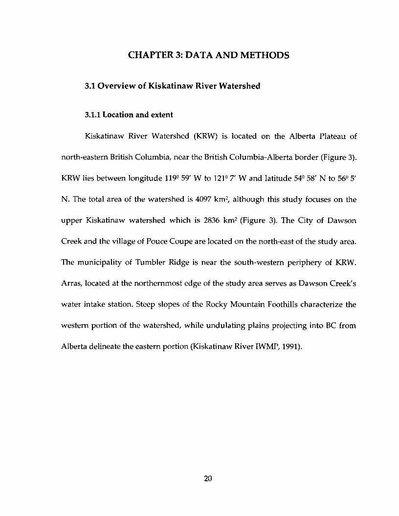


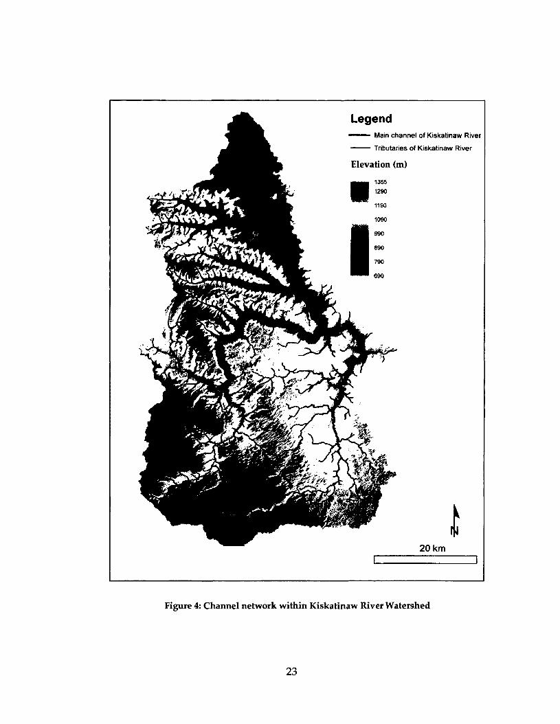


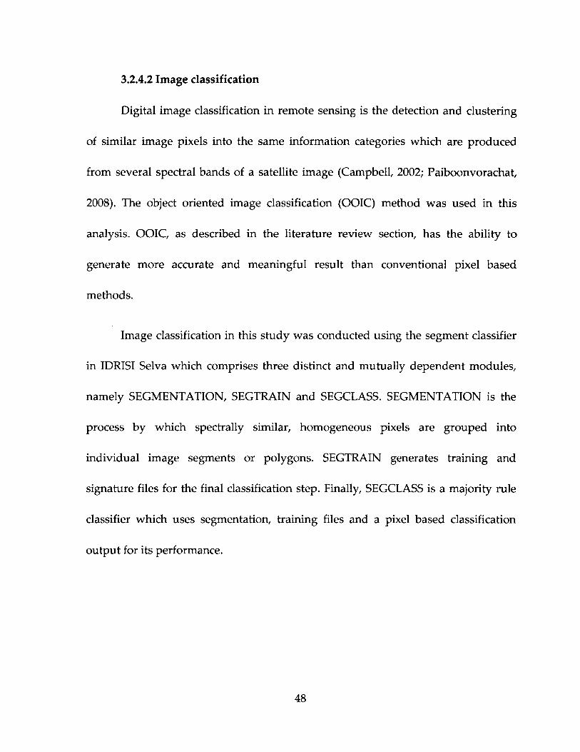


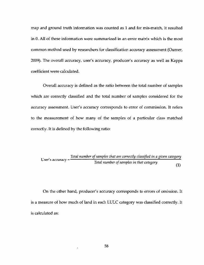


![A [simple] land cover change intercomparison](https://static.documents.pub/doc/80x56/56814f92550346895dbd4da4/a-simple-land-cover-change-intercomparison.jpg)


