ANALYSIS OF NUCLEAR REACTOR PERIOD MEASUREMENTS by LAURENCE LESLIE MOON A THESIS submitted to OREGON STATE UNIVERSITY in partial fulfillment of the requirements for the degree of MASTER OF SCIENCE June 1963
Transcript
ANALYSIS OF NUCLEAR REACTOR PERIOD MEASUREMENTS
by
LAURENCE LESLIE MOON
A THESIS
submitted to
OREGON STATE UNIVERSITY
in partial fulfillment of the requirements for the
degree of
MASTER OF SCIENCE
June 1963
APPROVED
----~-
Associate Professor of Electrical Engineering
In Charge of Major
Chairman of School Graduate Committee
Date thesis is pre s e nte d_--=gtE=--(~_1_middot_zmiddot_plusmnL_~I_1~0-=_____
Typed by Carol Baker
ACKNOWLEDGMENT
My special thanks go to Associate Professor Robert R
Michael for his helpful suggestions and encouragement during
the research for this paper The efforts of Assistant Professor
Edward A Daly made the reactor experiment possibl e
TABLE OF CONTENTS
Page INTRODUCTION l
INTRODUCTION TO REACTOR MEASUREMENTS 2
Basic Concepts 2 Reactor Kinetics 4
NUCLEAR REACTOR FLUCTUATIONS 7
Statistical Terms 8 Nature of the Fluctuati ons 10 Radioactive Decay Statistics 11
EXPERIMENTAL DETERMINATION OF REACTOR FLUCTUATION DISTRIBUTION 13
Simple Power Measurement 21 Reciprocal Period Measurement 30 Operating Parameters 35 Quasi-continuous Measurement 36
GENERATION OF RELIABLE PER IOD SCRAM 41
Basic Increase Function 41 Optimum Increase Function 44 Weighted Increase Function 47 Comparison of Measurement Types 50 Design of Optimum Period Scram Device 51 Maximum Acceptable Accuracy Values 52 Quasi -continuous Measurement 56
COMPARISON OF ANALOGUE AND DIGITAL PERIOD DEVICES 70
CONCLUDING COMMENTS 72
BIBLIOGRAPHY 74
LIST OF TABLES AND FIGURES
Table Page
1 Reactor Test Results 15 2 Per Unit Deviation of Reciprocal Period
Measurement 40
Figure 1 Accuracy of Count Rate Measurement 26 2 Accuracy of Count Rate Measurement 29 3 Reciprocal Period Indication Ratio 32 4 Accuracy of Reciprocal Period Measurement 34 5 Accuracy of Reciprocal Period Measurement
as a Function of Counting Time 38 6 Accuracy of Basic Increase Function
Measurement 43 7 Magnitude of Vincent s Optimum Increase
Function 46 8 Accuracy of Weighted Increase Function
Measurement 49 9 Illustration of Accuracy Parameter 54
10 Typical Analogue Period Meter 61 J 1 Transient Response of Analogue Period Meter 63 12 Steady State Accuracy of Analogue Period Meter 68
ANALYSIS OF NUCLEAR REACTOR PERIOD MEASUREMENTS
The production of power in a nuclear reactor involves complex1
dynamic processes which require censtant observation to assure
safe efficient utilizat ion These observations consist of measure shy
ments to determine such thing s as power levels control rod posishy
tiona temperatures and others depending upon the size and comshy
plexity of the reactor The statistical nature of the processes in-
valved complicates these measurements This paper is concerned
with one type of measurement that which determines the rate of
change of reactor power
The time rate of change of power is usually expressed in terms
of the period of the reactor This is the time taken for the power
to change by a factor e (the base of natural logarithms) Assuming
the reactor response to be exponential the reciprocal of the period
is the coefficient of time in t he e xponent of e Careful control of
the period is necessary particularly on start up to prevent rapid
power increases It is essential for reasons of safety that the reshy
actor not be allowed to become critical with prompt neutrons alone
Monitoring the period is an effective way to prevent this
Common period measuring systems are analogue devices whose
performance is limited by factors inherent in the devices themshy
selves and by statistical fluctuations Direct comparison of the
2
performance of an analogue device with that dictated by statistical
limitations has not been published Once this comparison is made
the feasibility of a digital device can be determined The object of
this paper is to make this comparison
INTRODUCTION TO REACTOR M EASUREMENTS
Some knowledge of the behavior of a nuclear reactor is required
before one can attempt to analyze devices used for reactor measureshy
ments It is not intended that a lengthy description of reactor
physics and kinetics be given here standard textbooks and referenshy
ces are to be consulted
Basic Concepts
A nuclear reactor might be de scribed as a system for controlshy
ling a neutron chain reaction Neutrons created during the fission
of certain heavy nuclei survive to initiate fission in other heavy
nuclei When the ratio between the number of neutrons created in
one generation and those created in the generation immediately preshy
ceding is exactly unity the reaction is self sustaining This ratio is
called the effective multiplication factor K e
Each fission event releases energy which is distributed among
fission fragments neutrons neutrinos and decay gamma rays beta
particles and alpha particles A total of about 201 Mev is released
3
in the fission of uranium 235 of which about 190 Mev can be
1 d 1 If a filtCed amount of energy per fission is made availableuhtze
and transferred to the reactor as heat power the power level is
directly related to the fission rate The exact correlation depends
upon the degree of equilibrium between fission product production
and decay and upon the fraction of gamma rays which escape from
the reactor (24 p 5 )
It will be assumed that reactor power is directly proportional
to the fission rate This is a basic assumption upon which importshy
ant nuclear measurement techniques are based Thus the reactor
2power can be found by determining the fission rate
The neutrons in a reactor are distributed throughout the core
with a distribution of energy and direction A convenient quantity
in this regard is the neutron flux ~ with the units neutrons per
square centimeter per second This is the ratio between the reacshy
tion rate per unit volume and the macroscopic cross section 24 p
23 )
The fission rate may then be determined by measuring the flux
This is frequently done using a detector filled with a suitable gas
1 The neutrinos carry about 11 Mev from the system
2 Murray states that 3 3 x 1o1 0 fissions of uranium 235 per second are necessary for the production of 1 watt of reactor power (24 p 5 )
4
Neutrons passing through the detecter collide with constituents of
the gas creating ionizing particles The ions and electrons created
by these secondary particles are rapidly swept to electrodes by a
strong electric field A voltage pulse at the detector output is the
result The number of pulses per unit time is proportional to the
flux at the detector location Another type the ion chamber gives
a current output proportional to the flux These devices are
descr ibed in the book by Price (26 chapter 9)
It is assumed when making neutron flux measurements that
the d e tec tor output is directly proportional to the reactor power
This means that the flux at the detector location usually a region of
relative ly low flux near the core periphery is representative of the
high core flux It is a problem for the reactor designer to select
detector locations where the assumption of proportionality between
detector output and reactor power is valid Spatial flu~ distribushy
tions in the reactor may require the use of several detectors whose
outputs are combined in some manner to give the reactor power
Reactor Kinetics
As the power level detector is triggered by neutrons it is desirshy
able to hav e some knowledge of the time behavior of neutron flux
A pair of equations developed from a space independent model
which considers only one neutron energy group are commonly used
5
to determine the neutron density 19 p 86) An average flux is
then obtained by multiplying this density value by the mean velocity
of the group considered These equations are
6
1 dndt = (eKe - (3Ke)nL + I Xiyici and
i=l
2 de dt = 3 K nL - X c 1 1 e 1 1
In equations 1 and 2
n is the neutron density
Cmiddot1 is the density of the ith precursor
K is the effective multiplication factor e
oKe is the
L is the prompt neutron lifetime
is the fraction of neutrons due to the ithl3i precursor
3 is the total de layed neutron fraction
x_ 1 is the decay constant of the ith precursor
y is the effectiveness of ith precursor neutrons1
in producing fission as compared to prompt neutrons
If an artificial fast neutron source is present sf is added to equashyf
tion 1 with S being the source strength and f the fraction of source
6
neutrons which do not escape from the system (24 p 166)
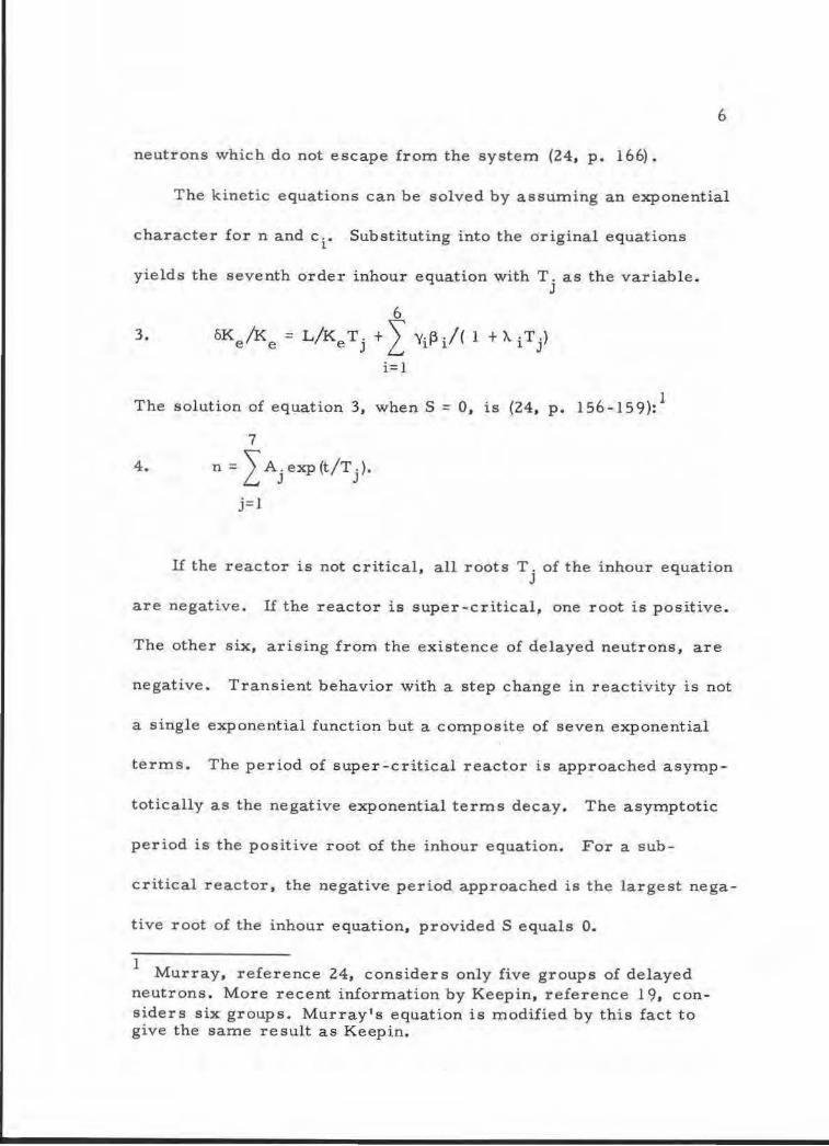
The kinetic equations can be solved by assuming an exponential
character for n and c Substituting into the original equations1
yields the seventh order inhour equation with T as the variable J
6 3 oK K = LKeTJ + Yf3 j( 1 + gt middotT )e e Ltl lJ
i~l
1The solution of equation 3 when S = 0 is (24 p 156-159)
7
4 n =A exp (tT )L J J
j= 1
lf the reactor is not critical all roots T of the inhour equationJ
are negative If the reactor is super-critical one root is positive
The other six arising from the existence of delayed neutrons are
negative Transient behavior with a step change in reactivity is not
a single exponential function but a composite of seven exponential
terms The period of super-critical reactor is approached asympshy
totically as the negative exponential terms decay The asymptotic
period is the positive root of the inhour equation For a sub-
critical reactor the negative period approached is the largest negashy
tive root of the inhour equation provided S equals 0
1 Murray reference 24 considers only five groups of delayed
neutrons More recent information by Keepin reference 19 conshysiders six groups Murrays equation is modified by this fact to give the same result as Keepin
7
The assumption that a single exponential function is a good
approximation to the complete solution of the inhour equation is
implicit in period measuring devices Toppel has calculated the
time required after a step change in reactivity for the difference
between the asymptotic reciprocal period obtained from the inhour
equation and the value obtained from the single exponential approxishy
mation to become less than a specified fraction of the asymptotic
value (28) This waiting time can be as long as one period in a
source free reactor when the asymptotic period is about 10 seconds
or less (28 p 91 and longer in reactors containing sources (28
p 96) Discussion of the effect of the single exponential approxishy
mation on period measuring devices is beyond the scope of this
paper It will be assumed that this approximation is sufficiently
valid to permit useful period measurements to be made
NUCLEAR REACTOR FLUCTUATIONS
A moment 1 s consideration will show that even in a reactor
operating at a steady power level the neutron flux must fluctuate
with time The various processes by which neutrons interact with
nuclei are described by cross sections (24 p 20) Cross sections
are a measure of the probability of occurrence for a given reaction
and their magnitude is a function of neutron energy Fission
8
neutrons are not created with a fixed energy but with a distribution
of energy (24 p 38) Likewise thermalized neutrons do not have a
fixed energy (24 p 30) A fixed number of neutrons is not created
in a fission (1 0 ) one must consider the probability that a given numshy
ber are created The number of collisions with moderator nuclei
required to thermalize fission neutrons is not a constant but will
vary from one neutron to another due to variations in the scattering
angle (24 p 37 )
The energy of neutrons in a reactor varies over a large range
with a certain probability for a given number lying in a given range
The various processes occurring within the reactor must be deshy
scribed by energy dependent probabilities Because of these facts
average values are used when reactor behavior is discussed Mean
thermal neutron energy mean fission neutron energy mean neushy
tron lifetime and mean number of collisions to thermalize are
terms frequently used
Statistical Terms
In this paper we are interested in the nature of the neutron flux
fluctuations Before discussing this further it would be well to de shy
fine several statistical terms which will be encountered frequently
It must be recognized at the outset that the shape of the curves
showing the results of experiments performed on statistical
9
processes need not be the same Several types of statistical proshy
cesses have been mathematically described in terms of the form of
the experimental results
The basic mathematical description is the probability density
function p(x) (22 p 419-421) To find the probability of obtaining
a result within certain limits p (x) is integrated between those limshy
its This density function is normalized to make the area u nder its
curve unity The variabl e x may be discrete or continuous depend shy
ing upon the process i n question
The probability distribution function P (x) is the integral of the
density function p (x) from negative infi nity to x It expresses the
probability of obtaining a result less than x (22 p 428)
SX
5 P (x) ~ p (x )dx
-00
The familiar normal distribution is an example (22 p 439)
1 2 6 P (x) = (1CJ~) exp - (x- M )
za2
Values of the normal and other distribution functions are tabulated
(5 8 21 25)
Of special1nterest are the average properties of the process
These are found from the moment functions of mth order (22 p
456)
10
S00
7 Mm (x) = xmp (x)dx
-00
The moment function gives the expected value of xm For example
the first moment (m equals one) is the mean and the second moment
is the mean square of the process
2 The variance ltY a common measure of the spread of a distri shy
bution is the second central moment Central moments are obshy
tained by biasing ordinary moments by the mean of the distribution
(22 bull p 4 57 ) bull
00
8 C m (x) = S[x - M 1 (x)Jm p (x) dx
-00
It can be shown that the variance is the difference between the mean
square and the mean squared (22 p 459)
2 1 29 ()2 (x) = M (x)- [M (x) ]
Nature of the Fluctuations
The information of interest here is the type of distribution folshy
lowed by the reactor fluctuations Some theoretical trea tment has
been given to reactor fluctuations in the literature (7 9 13 14
17 ) Two papers present a thorough theoretical treatment considshy
ering a sub-critical reactor as a stationary random process (7 14)
11
The term stationary refers to a process whose statistical charactershy
istics are not time dependent (22 p 417) The term random reshy
fers to a physical process containing a random element (3 p 1 )
The mathematical techniques used are in the realm of advanced
mathematical statistics and will not be considered here However
the assumption that the process is random and stationary seems unshy
duly restrictive Harris (14 p 30) feels that a critical reactor
will not be a random process and that in any case the counting sys shy
tem c a n n ot be stationary Clark 1 feels that a reactor is a Markov
rather than a random process The methods used with Markov proshy
cesses account for a lack of statistical independence in the system
studied In a reactor the neutron flux at any given time is related
to the flux extsting earlier and some statistical dependence must
be present
Radioactive Decay Statistics
With the lack of a theoretical result suitable for engineering
purposes it was necessary to develop a model which would lead to
a readily applicable result The first one which comes to mmd is
the decay of radioactive nuclei
The stati stics of radioactive decay are discussed by Price (26
1
Mr R G Clark Hanford Atomic Works private communication
12
p 53-56) He states that the distribution followed is the binomial
distribution (26 p 55) If the number of nuclei decaying in a given
time interval is much less than the total number present at the
start of the interval and if the product of the decay constant and
time interval is much less than unity the simpler Poisson distrishy
bution is an excellent approximation Decay statistics are comshy
monly assumed to follow the Poisson rather than the binomial
distribution
The Poisson distribution is characterized by the following
probability density function (31 p 67 )
u X
exp (-u)10 p (x) = x
In equation 10 xis a discrete variable Calculation of the first
and second moments shows that the mean and variance of the distrishy
bution are both equal to u (31 p 203 )
The assumption that a process follows a Poisson distribution
is very convenient Only one parameter u is required to comshy
pletely describe the process No separate calculation to find the
variance is necessary
13
EXPERIMENTAL DETERMINATION OF REACTOR FLUCTUATION D1STRIBUTION
An experiment to test the validity of assuming that a reactors
fluctuations follow a Poisson distribution was performed The re shy
actor at Oregon State University an Aerojet-General Nucleonics
AGN 201 was used This is a low power reactor designed for trainshy
ing purposes The lack of a general theory for reactor fluctuations
applicable to a critical reactor made experimentation necessary
Experimental Methods
The equipment and procedures used were essentially routine
A boron-trifluoride filled thermal neutron detector Radiation
Counter Laboratories model 10502 was installed in one of the reshy
actor loading ports The flux at the detector location was the order
of a hundredth of the maximum core flux (4 p 165 )1 Mechanically
coupled to the detector was a cathode follower circuit providing a
low output impedance to eight feet of coaxial cable transmitting de-
teeter pulses to Tracerlab RLI-1 linear amplifier A Hewlett-
Packard 524C electronic counter gave the output information
The detector was relatively insensitive to gamma rays A
The sensitive volume of the detector was located outside the graphite reflector and most of the lead shield The flux varies with distance from the center of the core so the detector output represhysents a spatial average
14
radium source placed adjacent to the detector resulted in the obsershy
vation of pulses no larger than 5 millivolts Using the shut down
reactor as a source of neutrons resulted in the observation of pulses
up to 60 millivolts In a high mtensity gamma ray field the small
pulses due to individual gamma rays can pile up to produce brger
pulses which can not be distinguished from those due to neutrons
(the neutron detector was used as a proportional counter j The deshy
tector was placed in the loading port with the reactor operating at
full rated power and a curve of count rate as a function of detector
voltage was obtained This curve showed a plateau of about 400
volts length with a slope of about l 25 percent per l 00 volts The
presence of this wide plateau is evidence that the gamma ray field
was not sufficiently intense to produce pile up effects (12 p 88)
Experimental Results
The results of this experiment and associated calculations are
shown in Table l Sarnple mean and sample variance characterize
the raw data The latter consists of a number of readings of counts
accumulated during a flxed time interval This was conveniently
done with the Hewlett-Packard 524C counter which would count for
a pre set interval hold the result for a fixed time then automatically
reset and resume cotAnting In all cases the reactor was as near a
condition of equilibrium as was possible to achieve
15
Table 1 Reactor Test Results
Nominal Counting Sample Sampl e Sample Sample Power Time Size Mean Variance_____________________________________________
1 1 mw 10 sec 25 128476 402552
2 1 100 13669 43016 3 II 0 I 100 13 13 2838
4 It 0 01 so 1 74 1 83
5 10 mw 10 25 987452 5567934
6 II 1 100 82570 1171 38
7 It 10 10 842690 1396121
8 II o 1 100 83 15 98 43
9 0 1 100 101 46 97255
10 II o 01 50 834 862
11 100 mw l 100 845056 1381221
12 II 1 24 811779 755956
13 0 l 25 85 7 12 69128 14 It 0 01 25 8564 5824
15 II o 01 100 8550 78 88
16 II 0 1 100 844 82 733 48
----------------------------------------------
16
1
Table 1 (Continued)
Data 2 2Sample Intervals Sample X Critical X
1 4 6 66 40 29
2 8 7771 124 12
3 7 6976 124 12
4 4 10 97 6369
5 2 0 04 41 64
6 11 1185 124 12
7 2 0554 18 48
8 7 1o 69 124 12
9 4 133 1 12 4 12
1o 6 938 6369
11 7 1280 124 12
12 4 0 7 01 40 29
13 3 0 356 4029
14 4 1 61 4164
15 12 888 12412
1 6 9 7 95 124 12
Critic al values taken at 1 percent significance level (8 p 232) 1
17
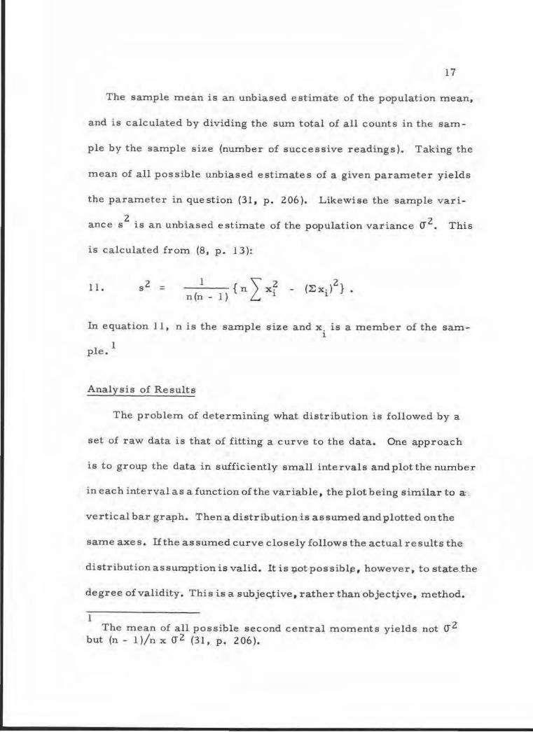
The sample mean is an unbiased estimate of the population mean
and is calculated by dividing the sum total of all counts in the samshy
ple by the sample size (number of successive readings) Taking the
mean of all possible unbiased estimates of a given parameter yields
the parameter in question (31 p 206 Likewise the sample varishy
ance s 2
is an unbiased estimate of the population variance cr 2 bull This
is calculated from (8 p 13)
11 --1 -- n x
1n(n - 1) L
In equation 11 n is the sample size and x is a member of the samshyi
1ple
Analysis of Results
The problem of determining what distribution is followed by a
set of raw data is that of fitting a curve to the data One approach
is to group the data in sufficiently small intervals and plot the number
in each intervalas a function of the variable the plot being similar to a
vertical bar graph Then a distribution is assumed andplotted on the
same axes Ifthe assumed curve closely follows the actual results the
distribution assumption is valid It is 9-otpossibl~ however to state the
degree of validity This is a subjective rather than object~ve method
The mean of all possible second central moments yields not o-2 but (n- 1)nx o-2 (31 p 206)
1
18
Statisticians have developed an objective method the chi-
squared (X 2 ) test (8 p 83-88 31 p 238-242) This involves
calculating the X 2 statistic for each sample and comparing it with
tabulated values at a stated significance level If the sample x 2 is less
than the tabulated X 2 the assumption is considered valid The statisshy
2tic X compares the actual and assumed relative frequencies (occurshy
rences per interval compared to total occurrences)
2The X statistic with r - 1 - g degrees of freedom is found from
the following relationship (8 p 85 )
r 2 - ei)
12 x2 =I (nishy
e 1
i=l
In equation 12 ni is the actual number of occurrences in the ith inshy
terval ei is the assumed number of occurrences g is the number
of assumed distribution paramete r s based upon the data and r is
the number of intervals
The sensitiveness of this test de)ends upon the number of
intervals r If a small enough number of intervals is used almost
any assumption will pass the test On the other hand if r is so
large that the assumed number of occurrences per interval is very
2small unrealistically large X values result There is no way to
explicitly surmount these difficulties However both references
consulted are agreed that the minimum number of assumed
19
occurrences per interval should be five
The sigmficance level sets the likelihood that a true assumption
will be rejected (8 p 16 ) For example if a 1 percent significance
level is chosen a true assumption will be accepted in 99 percent of
the tests on the average
Values of x2 were calculated for each sample assuming a
Poisson distribution with a mean equal to the sample mean These
values are compared to the critical values taken from the table (8
p 232) at the 1 percent significance level The table contains valshy
ues only for 100 degrees of freedom (df or less taken i n intervals
of 10 past 30 The df for most samples fell between tabulated valshy
ues When that was the case the next lowest tabulated value was
used This gave pessimistic values for the critical X 2 values
The Poisson table used to find the expected number of occurshy
rences per interval considered mean values only to l 00 If the
sample mean was less than 100 the assumed Poisson mean was the
nearest integer (but for sample 4 where 1 70 was assumed) to it
When the sample mean was greater than 100 a normal distribution
with mean and variance equal to the sample m ean was assumed
The Poisson distribution can be approximated by a normal disshy
tribution if the mean is sufficiently large Price considers a mean
of 100 or greater sufficient to make the normal approximation to the
20
Poisson distribution valid (26 p 57) Since the normal distribution
is more thoroughly tabulated than the Poisson distribution this
approximation is often convenient
The raw data and chi- squared test calculations are too lengthy
to include in the paper
Conclusion
The assumption of a Poisson distribution or an approximate
normal distribution for nuclear counting fluctuations is both convenshy
ient and widespread Table l shows the results of the chi- squared
test performed upon reactor counting data with this assumption All
samples but one number 9 pass the test This indicates that the
Poisson distribution assumption is valid within the meaning of the
chi-squared test Table 1 does not indicate that a Poisson distribushy
tion is the only or even the most accurate assumption Even with
an objective test judgement must be used in reaching a final conshy
number of intervals relation between sample and critical chi shy
squared values experimental methods and perhaps others
For example consider the very small X 2 values obtained in
samples 5 7 and 13 Only two or three intervals were possible
with the small sample size These results should not be given the
same weight as the larger but still relatively small X 2 values in
21
samples 15 and 16 On the other hand the large x 2 value of sample
9 might be discounted as the one in a hundred which gives a negative
result with a true assumption The only difference between samples
8 and 9 is the linear amplifier gain (more small pulses are counted
in sample 9) and sample 8 has a relatively small X 2 value
On the basis of the results shown in Table 1 nuclear reactor
fluctuations as seen by counting device will be assumed to follow a
Poisson distribution in this paper
STATISTICAL LIMITATIONS UPON MEASUREMENT
Consecutive measurements made during a finite time interval
of some property of a statistical process will rarely be identical
This is a direct result of the fact that the property in question
1fluctuates about some mean value The measured fluctuation will
be relatively smaller than the instantaneous process fluctuations due
to averaging inherent in the finite time interval measurement To
reduce relative fluctuations a longer time interval (larger sample
size) must be used
Simple Power Measurement
The count rate of a pulse type neutron detector is proportional
1 The independent variable is not necessarily time but iq this
paper it is the only one considered
22
to reactor power if the detector is properly located Ipound a mean
count rate r exists the fluctuations in the count rate are
J 3 () 2 = t
r c
when the fluctuations follow a Poisson distribution (26 p 59)
Note that the fluctuations exist in the number of events n = rt that c
occur during the time interval t rather than in the events per unit c
time r
The variance in the number of counts per interval n may be
equal to n only when the count rate is constant during the counting
inter val Price shows that this variance is n exp (- t ) for radioshyc
active decay when the counting time tc is not small enough to make
tc lt lt 1 (26 p 56) In an analogous manner equation 13 is mulshy
tiplied by exp (tcT) when tc is not much smaller than the period T
of an exponential increase
Equation 13 for the count rate variance neglects any fluctua shy
tions in the counting time t which must exist with any physicalc
measuring device In order to determine how the counting time
fluctuations affect the result the rule for combining vanances in
an equation containing fluctuating quantities must be known The
answer is provided by the Motorola handbook (23 section 3 2 4
p 5 ) Ipound y is a function of x X x then the variance in y1 2 n
23
is found from equation 14
Applying equation 14 to count rate fluctuations where = ntc
the following result is obtained when the count rate is constant
2 - 2 -2 4 215 () r = nfc + (n tc )0 t
c
2 Equation 13 will be valid when crt is small enough to make the
c second term in equation 15 much smaller than the first term If the
first term is to be larger by a factor F the following inequality must
be satisfied
2 16 () lt t
2 I F t c c
Only when the counting time is the same order of magnitude as 0t
will the counting time var iance be important The inherent accushy
racy of a measurement in a region where the counting time variance
is important will probably be so poor as to discourage the measureshy
ment
As an example of what is possible with a sophisticated device
the Hewlett-Packard 524C counter contains a highly stable (5 parts
8in 10 per week) 1 megacycle standard oscillator The timing error
can be as large as one period of the standard oscillator plus the
c
24
stability due to uncertainties in the gating circuits or about 1
microsecond This is small enough to consider the result of equashy
tion 1 3 or the first term of equation 15 as a good approximation
which will be used throughout this paper
If the statistical distribution is specified a known relationship
exists between the reliability and the standard deviation This reshy
lationship is found in the table for the given distribution The reshy
liability is the probability of obtaining a result within the specified
number K of standard deviations from the mean Accuracy then
expresses the relationship between the magnitude of K standard
deviations and the mean in percent Both reliability and accuracy
must be specified for a given measurement one can not be specified
independently of the other
For example 95 percent of the observations from a normal
distribution fall within 1 96 standard deviations of the mean If the
mean is 100 and the variance is unity the measurement would be deshy
scribed as having an accuracy of 1 96 percent ata reliability of 0 95
The per unit deviation P U D or the ratio of the standard
deviation to the mean is often found mathematically Accuracy at
a specified reliability is then 1 OOK (P U D )
With this knowledge it is possible to find the relation between
counting time mean count rate and accuracy for a simple power
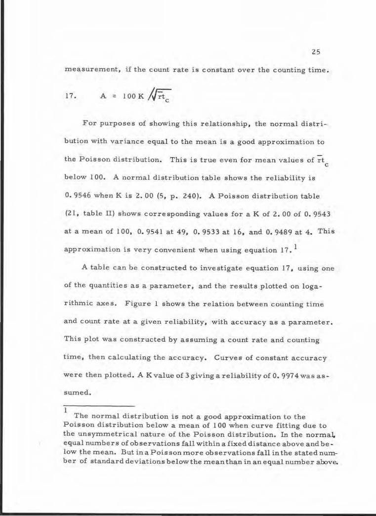
25
measurement if the count rate is constant over the counting time
17 A == 100 K Jtc
For purposes of showing this relationship the normal distrishy
bution with variance equal to the mean is a good approximation to
the Poisson distribution This is true even for mean values of rt c
below 100 A normal distribution table shows the reliability is
0 9546 when K is 2 00 (5 p 240) A Poisson distribution table
(21 table II) shows corresponding values for a K of 2 00 of 0 9543
at a mean of 100 0 9541 at 49 0 9533 at 16 and 0 9489 at 4 This
1approximation is very convenient when using equation 17
A table can be constructed to investigate equation 17 using one
of the quantities as a parameter and the results plotted on logashy
rithmic axes Figure l shows the relation between counting time
and count rate at a given reliability with accuracy as a parameter
This plot was constructed by assuming a count rate and counting
time then calculating the accuracy Curves of constant accuracy
were then plotted A K value of 3 giving a reliability of 0 9974 was asshy
sUcmed
1 The normal distribution is not a good approximation to the
Poisson distribution below a mean of 100 when curve fitting due to the unsymmetrical nature of the Poisson distribution In the normal equal nUcmbers of observations fall within a fixed distance above and beshylow the mean But inaPoissonmore observations fall in the stated numshyber of standard deviations belowthe mean than in an equal number above
26
1o- 1
(x5)
(x2)
-3 10
10 perce t
Mean C ount Rate r Counts Per Unit Time Interval
Figure 1 Accuracy of Count R ate Measurement
gtshy~ ~ Q)
~ s Q)
gt l)
Q)
8 ~ ~ s
0
27
The accuracy value increases as the counting time becomes
smaller the increase being inversely proportional to the square
root of counting time at a fixed count rate The counting time can
be decreased until the uncertainty becomes several times larger
than the true count rate There exists some minimum counting
time for a given count rate below which even an order of magnitude
estimate of the count rate is impossible~ The lower left corner of
Figure 1 represents a region of impossibility It is difficult to deshy
fine the boundaries of this region as the normal approximation to
the Poisson becomes poorer as rt becomes smaller The 300 pershyc
cent curve appears to be a reasonable boundary however
The effect of a lower reliability parameter is to improve the
accuracy (lower the numerical value) by the ratio of K values at a
given counting time and count rate The ordinates of Figure 1 are
directly proportional to K
All curves of Figure 1 were plotted with the assumption that the
normal distribution is a good approximation to the Poisson distribushy
tion witll the exception of the 100 percent curve Using linear inshy
terpo1ation the Poisson distribution table (21 table II p 11) gives
a K of about 3 16 for a reliability of 0 997 4 The normal distribushy
tion gives counting times about ll percent smaller than those shown
for the 100 percent curves The use of the normal distribution
28
approximation for the 300 percent curve is questionable as 9974
percent of observations from a Poisson distribution fall within
minls l and plus 5 15 standard deviations of the mean when rt is c
unity If an average K of 3 07 5 is taken the Poisson distribution
curve for 300 percent accuracy is essentially that plotted The difshy
ference between exact and approximate curves is not significant for
thE r emainder of those shown in Figure 1
Figure 1 is similar to a plot developed by Hoehn (16 p 1 08)
to show the time required to measure electric current to a given
accuracy He derives an equation considering current as a Poisson
distributed flow of charge from which his plot is developed The
elementary probability theory used in this paper will reproduce
Hoehns results This leads to the inference that a curve similar
to Figure 1 may exist for any physical measurement and that a
r egion of impossibility may be encountered
Another useful demonstration of equation 17 is a plot showing
the relation between accuracy and the mean number of events rt c
which occur during the counting interval Figure 2 is such a plot
Several different reliability values are used to show the effect of
reliability upon accuracy A normal distribution is assumed for
convenience Presenting equation 17 in this manner emphasizes
the fact that it is not the count rate but the number of events
~ Q)
u 1-lt Q)
P
Cil u (x2)Cil 1-lt l u u 0
-ct 10
----1-----tshy-shy- - - ---~~-----~
74
10 (x2) (x5)
Mean Number of Events Per Counting Interval rtc
Figure 2 Accuracy of Count Rate Measurement
30
occurring in the counting interval that determines the accuracy of
the measurement
Reciprocal Period Measurement
The preceding section discussed the statistical fluctuations
involved in measurements of count rate Figures l and 2
show the relative magnitudes of these fluctuat ions when the count
rate is constant The quantity of interest in this paper is not reacshy
tor power but reactor period Two power measurements can be
combined to yield an indication of reciprocal period The accuracy
of a reciprocal period measurement can be no better than the
power measurements f rom which it is made
U the reactor power varies in an exponential manner so does
the count rate r The reciprocal period 1T is then defined by
equation 18
18 1T = 1r x drdt
This is found by d1viding the slope of the count rate-time curve
by the count rate The slope R can be approx imated by equation 19
If the comparison time ~t is much longer than the counting times
used to determine r 1 and r bull the count rates can be assumed2
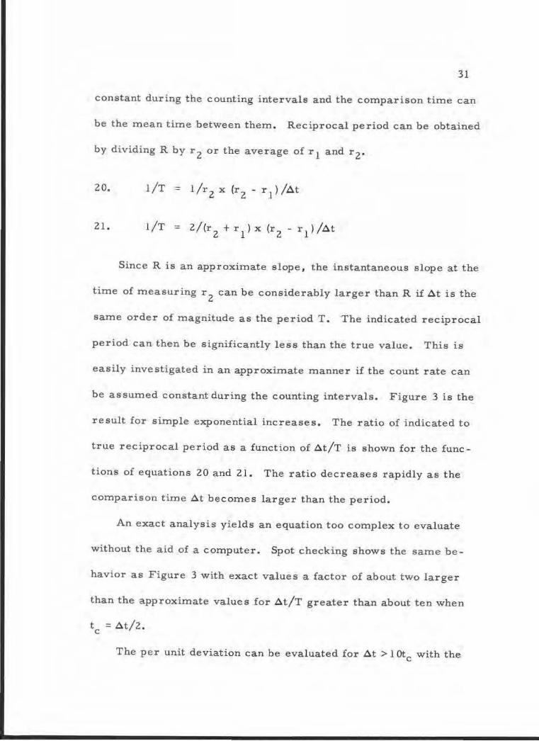
31
constant during the counting intervals and the comparison time can
be t he mean time between them Reciprocal period can be obtained
by d ividing R by r 2 or the average of r and r bull1 2
20 liT = llr x(r -r )1At2 2 1
21 1IT = 2I (r + r ) x (r - r ) IAt2 1 2 1
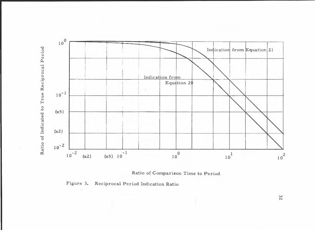
Since R is an approximate slope the instantaneous slope at the
time of measuring r can be considerably larger than R if At is the2
same order of magnitude as the period T The indicated reciprocal
period can then be significantly less than the true value This is
easily investigated in an approximate manner if the count rate can
be assumed constant during the counting intervals Figure 3 is the
result for simple exponential increases The ratio of indicated to
true reciprocal period as a function of AtiT is shown for the funcshy
tions of equations 20 and 21 The ratio decreases rapidly as the
comparison time At becomes larger than the period
An exact analysis yields an equation too complex to evaluate
without the aid of a computer Spot checking shows the same beshy
havior as Figure 3 with exact values a factor of about two larger
than the approximate values for AtiT greater than about ten when
tc = Atl2
The per unit deviation can be evaluated for At gt 1Otc with the
10deg U 0 1-4 Q)
~ ro u 0 1-4 P u Q)
~ Q) 1o- 1 l H ~
0 jgt
U (x5) Q)
jgt
ro u
U H ~ (x2)
0
0 jgt 10- 2 ro
I
I I
--~
I
l I I l
I
l
I i
I
i I
I I
I j I
I
i
I
I
----r-- ~
~nc
Indicat
ion from ~~I Equ tion 2
I
I
from ~quationicatior I
~~ ~
i
~ ~
21
~ ~middot
~ -2 -1 0 1 210 (x2) (x5) 1 0 10 10 10
Ratio of Comparison Time to Period
Figure 3 Reciprocal Period Indication Ratio
w N
33
method of equation 14 The restrmiddotiction on tc simplifies the matheshy
matics since the count rate can then be assumed constant over the
counting intervals Little difference exists between exact and apshy
proximate values when tc is sufficiently small
The result for the function of equation 20 is given 1n equation
22 Likewise equation 23 expresses the per unit deviation of the
function of equation 21 These equations neglect fluctuations in the
counting and comparison times
222 P U D = l(2 - 1) X (1tc1) + (12) (2tc 2)
2 3 PUD = 2(2 + 1 )(2 1) x 12lt1tc2+r2tc1)
These per unit deviation functions were converted to accuracy
functions at a reliability of 0 997 4 Figure 4 is a plot of accuracy
as a function of the ratio 6tT with t and - specified (counting c 1
times do not have to be equal but considering them equal sirnplishy
fies the calculations) The values specified are t = 0 01 minutes c
3 and r 1 = 1 0 counts per minute The subscripts on r refer to the
first and second counting intervals which are used to determine
1T and the bar over r specifies that mean values are being
considered
1 10
C) 0 1-lt Q)
Poi 0 Q)
8 E-l ~ 0 tO 1-lt ro (x5)8 0 u
(x2)
- 1 10
-T l 32xl0 10 10
- ____ r----f---r---~ middotcat ion from ~quat ion 21r----F -l0
I dicatilt n from
~Equat ion 20 ~ ~ ~ountingTimesmiddot001 11kinutes ~ ~ean Ini ial Co~nt Rat e10 3 Pc r Min ~te Reliabili tv 0 9 g74
-
i i I
I I
I I I
I
~
~
~
Accuracy at Given Reliability Percent
Figure 4 Accuracy of Reciprocal Period Measurement
35
Operating Parameters
Time is important in a period measuring system particularly
if warning of excessive periods is de sired There is apparently no
published information which enables specification of minimum
performance standards It seems reasonable however that an
upper limit to the useful comparison time is the order of one perishy
od Figure 4 then sets limits upon the counting time and count rate
if satisfactory accuracy is to be achieved Satisfactory accuracy
is difficult to define without operating experience but 10 percent
seems reasonable
Figure 4 shows that an initial count rate of 1o5 counts per minshy
ute is required to obtain 10 percent accuracy with 0 01 minute
counting times when the comparison time is one period Increasing
the counting times to 1 minute will also provide better than 10 per shy
3cent accuracy at an initial count rate of 10 counts per minute
The minimum period to be measured limits the maximum counting
time to one half its value if the reciprocal period indication is to be
obtained in ore period The maximum count rate obtainable from
a neutron detector is limited by its resolution time to the order of
6 7 110 or 10 counts per mmute A realist1c estimate of the
1 Price (26 p 126) states that the resolving time for Geiger tube
detectors is the order of 100 micrQseconds The neutron detector not utilizing avalanche multiplication should have a resolving time less than this value
36
minimum accuracy value obtainable in a reciprocal period measurshy
ing device is 10 percent at comparison times of 0 1 T and 1 percent
at comparison times of one period
Quasi-continuous Measurement
Once the measuring system has been in operation for a suffishy
ciently long time an output indication occurs every counting intershy
val If the counting time is small the measurement is almost conshy
tinuous A possible mode of operation involves comparison of sucshy
cessive counting intervals with no time separation between them
It may be also desirable to obtain the most accurate measurement
possible in a given time Figure 4 can be extended to show accurashy
cy as a function of counting time when the two counting intervals
are of equal length
The approximations used in the developrnent of equations 22
and 23 result in relationships amenable to hand calculation whereshy
as a more exact analysis produces a result too complex for practishy
cal extensive investigation by hand To find the counting times
which produce the most accurate measurement it would be best to
use a more exact analysis instead of Figure 4 The exact results
are not greatly different from Figure 4 however
Equation 24 showing the per unit deviation of a reciprocal
period measurement obtained in the manner of equation 21 is not
37
restricted by the assumption of constant count rates during the
counti ng intervals An exponential increase of period T is initiated
at t = 0 when the count rate is r bull The measurement is completed0
at time t the counting intervals are of length t and the comparishyc
son time At is t - t bull c
tc IT 2e
24 PUD = - tc 1T t J T tc I T
(etIT-etc IT) )(e +e )r T(l-e0
Count rate variance is taken as exp (tcT )tc since the count rate
may not be constant over the counting intervals Variances in
counting time and comparison time are neglected
Figure 5 shows the accuracy at a given tT of unity and reliashy
bility corresponding to three standard deviations The results of
3Figure 4 for T = 0 1 minutes and r = 10 counts per minute are 0
shown to compare exact and approximate results The approxishy
mate values are as much as 12 or 15 percent lower than exact
values for t gt 0 lt When t is smaller than this the difference is c c
not significant
The most significant aspect of Figure 5 is the presence of a
minimum in the accuracy value The location of this minimum and
its magnitude are of interest However equation 24 is so complex
that setting the derivative to zero does not readily allow a solution
38
~ Q) 300 u J Q)
~
- 200 gt
-lt 150 Q
-lt Q) 100 ~ c Q) 75
gt j 50
gt u J I u
lt u 20
~ ~
E act AnalLrs1s~ Equa~ ion 2f4~L~r-shy ---p--~ 1Count middotng Time s o 0 Min ~tes
~ean nitial Cc unt Rc te 10 P Per Mi lute A pproxima e Anfal~sisRelial i1ity o 9~74
Ratio of Counting Time to Total Measurement Time tct
Figure 5 Accuracy of Reciprocal Period Measurement as a Function of Counting Time
39
for the counting time at which the -accuracy value is a minimum
A numerical approach using a computer should be attempted the
result would be of great practical interest The designer of a reshy
ciprocal period measuring device would want to obtain the most
accurate measurement possible and the knowledge of the counting
time at which this occurs would be helpful to him
Figure 5 shows that Figure 4 can be used to investigate recipshy
rocal period measuring devices over a large range of operating
c onditions keeping in mind that the accuracy values are optimistic
for large counting times
Table 2 shows the per unit deviation of reciprocal period
measurements predicted by equation 24 as a function of total
measurement time and counting time for several values of tT
Note that t c can be no larger than t2 The results are expressed
in terms of rr-T times per unit deviation rather than the per unit 0
deviation itself to avoid specification of operating conditions A
digit al computer could be used to construct a much more compreshy
h e nsive table
40
Table 2 Per Unit Deviation of Reciprocal Period Measurement
tT
0 1 0 05 II o 025 II o 01
o 5 0 25 II o 15 II 0 10 II o 05
0 01
1 0 5 n o 25 II 0 10 II o 05 II o 01
2 1 0 II o 5 II 0 1 II 0 OS
5 2 5 II 1 25 II 10 II 0 5 II o 1
10 5 0 II 25
tJTT x P UD 0
126 5 115 0 154 0
1o 40 9 80
10 20 12 45 25 1
3 89 3 14 3 74 4 86
1o 13
1 25 0 831 1 065 1 56
o 180 0 0541 o 0465 0 0357 0 0484
0 0136 o 00116
41
GENERATION OF RELIABLE PERIOD SCRAM
The limitations described in the preceding section suggest that
a method to obtain an indication of a dangerous period should be
use d rather than cont inuous monitoring of the period Figure 3
shows that the reciprocal period indication can be too low when the
comparison time is a period or longer Figure 4 and Table 2 show
the effect of statistical fluctuations on the measurement accuracy
Basic Increase Function
Indication of a dangerous period can be obtained by comparing
the difference between two count rate measurements to the standard
deviation of the first Let us call this the increase function as deshy
fined in equation 25
25 I = (r - r ) (T r 2 1 1
A compar i son time related to the shortest safe period is estabshy
lished If the increase in count rate during the comparison intershy
val is sufficiently large in comparison to the initial standard deviashy
tion the period is considered dangerously short Regardless of
the magnitude of the ratio of rate increase to initial standard deviashy
tion some false indications of excessive period will result The
larger the ratio the smaller the probability of fals e indications If
42
the ratio is 3 13 indications in 10 000 will be false (5 p 241 )
The variance of the increase function can be found in the
manner described by equation 14 The per unit deviation with the
result shown as equation 26 is then found
Equation 26 assume s that the count rate is constant during the
counting intervals and that variances in counting times and comshy
parison time are negligible Figure 6 relates accuracy to normalshy
ized comparison time at a 0 9974 reliability when the counting
times are 0 01 minutes and the initial count rate is 1000 counts
per minute Extension of Figure 6 to other operating conditions is
possible the ordinates are inversely proportional to the square
root of both initial count rate and counting time
An analysis more exact than that leading to equation 26 shows
the basic increase function to behave in a manner similar to Figure
5 as the counting time is varied Equation 27 is the exact solution
neglecting variances in counting and comparison times As with
equation 24 the counting time required for the minimum accuracy
value is of interest but difficult to find by hand calculation Figure
6 can be used to investigate a wide range of operating parameters
keeping in mind the fact that the ordinates are lower than the exact
0 j)
()
8 E-i ~ 0 Ill 1-lt 10deg roO 0 08 0 1-lt
()
u~ (x5) 0
0 j)
ro P= (x2)
-110 u 1 2 310 (x2) (x5) 10 10 10
Accuracy at Given Reliability Percent
lr----- I i I
I
I
i
[-_ i
I I
-
I I
~ I
Coulting Tirr
--
ate I ~ 3 PerM es 0 01 Mir utes
~ Meap Initialltf-OUnt I inute iReli itbility- 0 9974 ~ i
I ~II
II l ~ -middot-+--middot-----
~ I
F i gure 6 Accuracy of Basic Increase Function Measurement
44
values for long counting times
r-e-tc T_(e_t I_T_t_et_c ~ shy-1 _ _ -T )
27 P U D =
Comparison of Figures 4 and 6 will show the relative accurshy
acy capabilities of reciprocal period and basic increase function
measurements The reciprocal period meas urement has l ower
accuracy values over a wide range with the difference becoming
more marked as the comparison times become longer than one
period Basic increase function measurements do not suffer from
the limitation described in Figure 3 but offer no accuracy advan shy
tage over reciprocal p e riod measurements
Optimum Increase Function
However C H Vincent has shown that the magnitude of the
increase function can be made larger by weighting the data The
optimum weighting func tion has the same form as the equation
describing the time behavior of the count rate It is not necessary
to exactly fit the weighting function to the count rate equation to
obtain increase function value close to the maximum (29 p 183)
Vincent states that his result is the absolute optimum for this type
of measurement (29 p 183) His paper is quite thorough in deshy
veloping the optimum weighting function evaluating approximations
to it and suggests an analogue device to mechanize his result (29
p 185 ) He does not discuss the per unit deviation of his result
45
however stating that it will be no more than one part in I (29 p
1 91 )
Vincents optimum result with notation changed to that used
in this paper is shown as equation 28 (29 p 183)bull
Ot 2
28 1 = r sf(t) 2 dt 0
The time behavior of r is f(t) Applying this result to the case
where f(t) is an exponential f(t) = exp(OtT) Vincent obtains
equation 29 (29 p 184)
229 I r T = 12 [exp(OtT) -2]2 -1 +LnT
l
Vincents result equation 29 i s plotted in Figure 7 The
2quantities used r r T and OtT were chosen to pre sent the maxshy
1
imum amount of information on one plot Vincent plots this reshy
sult in a similar manner over a much narrower range (29 p 184)
The values for Figure 7 were obtained by assuming OtT and then
calculating 12r T from equation 29 with the aid of a slide rule and1
exponential table
Vinc ents mechanization of his optimum result i nvolves conshy
tinuous measurement of count rate using diode pump ratemeters
(29 p 185 ) This non-linear analogue device has weighting inshy
herent in its operation A scaling or counting device has no such
inherent weighting each pulse contributes a given amount to the
5xl 00
Q)
8
E-
1=1 0 I) (x5) 1-i ro 0 8 0 u
1o- 1 4 -4 3
I I I
I
I- I I
I I i
II I I
I _ I
----middot-t-i
middotmiddot-middot ----+-L---- ~----L----1I I middotmiddot- --middot-middotmiddot--- ---~--- -r
I l----~I I I
~ I - ----~ ----1---
I
--~~ I I I
2x l 0 5x l 0 l 0-
--
Magnitude Squared of Vincent s Optimum Increase Function Divided by the Product of Mean Initial Count Rate and Period I2rl T
F igur e 7 Magnitude of Vincents Optim um Increase Function
47
output regardless of its position in the counting interval A diode
pump ratemeter places more emphasis on events which have occurshy
red recently in time than on events occurring farther in the past
A digital measurement using counting devices can only approxishy
mate Vincents result
Weighted Increase Function
The basic increase function accuracy will be improved by
weighting r 2 before calculating the increase The lowest possible
accuracy value will be that corresponding to the measurement of
r 2 since multiplying a statistically fluctuating quantity by a con shy
stant does not alter its per unit deviation The weighted increase
function becomes the relationship of equation 30
30 Iw = (Wr - r )(J2 1 r 1
The per unit deviation of the weighted increase function will
approach that inherent in r 2 as W becomes larger According to
Vincents result W should be an exponential Equation 31 is the
per unit deviation of the weighted increase function obtained from
equation 30 by using equation 14 It is assumed that
r 2 = r 1 exp (~tT) and that variances in counting and comparison
times are negligible
48
J 2 ~tjT1 + W e
31 PUD =
The magnitude of equation 31 approaches the per unit deviation
of r 2 or j lr2tc Figure 2 then represent the lowest possible
accuracy values obtainable with a weighted increase function meas shy
urement Approach to within 10 percent of the optimum value for
6tT e qual to unity is possible if W is at least 4 6 and if W is at
least 38 a 10 percent approach is possible for a 6tT of 0 1 Setting
the weighting function at exp (3AtT )will give near optimum accuracy
for all 6tT greater than a few tenths
The ultimate accuracy of a weighted increase function measshy
uxement as predicted by equation 17 is shown in Figure 8 as a
function of comparison time To allow comparison with other
types of measurement investigated earlier in this paper the asshy
sumed parameters are a 0 01 minute counting time and an initial
count rate of 1000 counts per minute A simple exponential inshy
crease in count rate is assumed so that r =r exp (AtT )2 1
Figure 8 is an approximation good for counting times small
compared to the comparison time
Also shown in Figure 8 is the approximate curve for the
increase function weighted by exp (6tT ) with the same parameters
d 0 H Q)
P-t 0
4-gt
Q)
8 1-l I= 0 [J) H ro 0 8 0 (x5)u
(x2)
1 2
4
rease ~unctio ighted br e~p (
I
1 )
2xl0- 1 5x10- 1 10deg 10 1 ~ 102
Accuracy at Given Reliability Percent
Counting Times 0 01 Minutes Mean Initial Count Rate 1o3 Per Minute Reliability 0 997 4
Figur e 8 Accuracy of Weighted Increase Function Measurement
50
used in construction of the ultimate curve This weighting function
is an improvement over the basic increase function but falls short
of the ultimate over a wide range
Comparison of Measurement Types
To allow quick comparison between reciprocal period and inshy
c r ease function measurements the curves o f Figures 4 and 6 are
also shown in Figure 8 The reciprocal period curve is that corshy
responding to equation 21 For comparison times longer than one
period or so the r eciprocal period measurement is more accurate
than increase function measurements The ultimate weighted inshy
crease function measurement is much more accurate for shorter
comparison times The accuracy superiority of the reciprocal
period device may not be realized in practice due to the effect
described in Figure 3 setting an upper limit on the useful comparishy
son time
Figure 8 based on approximate analyses shows the relative
accuracy m e r its of two basic types of period related measurements
obtainable with digital mechanization A more exact approach not
restricted by the assumption of constant collnt rates during the
counting intervals has not been analyzed in detail for the various
measurements but should show the same relative behavior Figure
8 does not necessarily show the lowest possible accuracy values
51
Exact analysis shows the lowest possible accuracy values result at
some counting time the order of ~t4 A reduction by a factor of
two or three in the ordinates of Figure 8 is possible with longer
counting times for periods the order of 0 1 minutes Complete
solution of the exact relationships for the minimum accuracy valshy
ues would explicitly show the ultimate accuracy capabilities of the
various measurements
Design of Optimum Period Scram Device
Figure 8 shows the ultimate weighted increase function to have
an accuracy superiority over a large range of comparison times
No single equation will give the parameters for the optimum period
scram system using this function The designer can however
use Figure 8 as a guide in selecting counting times comparison
times and scram trigger level Several conflicting requirements
must be satisfied the system must be sufficiently fast accurate
reliable and free from spurious scrams
The shortest safe period determines the comparison time
but no explicit relation between the two is apparent As a rule of
thumb the reactor should be shut down within one period after the
start of an excursion Probably the slowest process involved is
withdrawing reactivity from the reactor In the Aerojet-General
AGN 201 reactor for example 54 percent of the reactivity
52
contained in the control and safety rods is withdrawn in 0 05 sec shy
onds from initiation of the scram (4 p 16) The rods excepting
the fine control rod are completely withdrawn in 0 12 seconds A
realistic estimate of the time for recognition decision and scram
is one second
Once the comparison time is fixed the counting time can be
selected Knowledge of the minimum accuracy counting time would
be helpful here If this is not known a trial and error procedure
using Figure 8 will approximately locate the minimum value
Every effort should be made to obtain as high a count rate as
possible for the sake of improving the accuracy Figure 8 shows
3 that 10 counts per minute are not sufficient to give satisfactory
accuracy for comparison times less than one period Much better
accuracy is obtained if the count rate is increased to 1oS counts
per minute Perhaps several detectors located in regions of dipoundshy
ferent neutron flux magnitudes should be used to give sufficiently
large count rates over a wide power range
Maximum Acceptable Accuracy Value
The term accuracy as used in this paper does not refer to the
11 11right or wrong nature of a measurement Rather it refers to
the magnitude of the spread of the measurement 1s distribution
53
This is very important as it determines the possibility of true and
false scrams
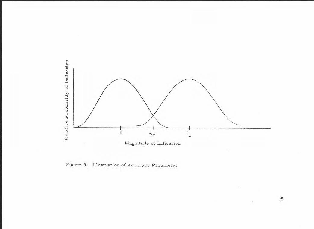
This situation is de scribed in Figure 9 The vertical axis
refers to the probability of obtaining a given I value plotted on the
horizontal axis If the power is steady the mean value of I is
zero but there is a definite p rob ability that non-zero values of I
will be measured Likewise if the power is increasing on the
critical period a value I results with a distribution determined byc
Figure 8
The location of the trigger level Itr fixes both the probability
of a true scram when the period is the critical value and the prob shy
ability of a false scram when the power is constant If the trigger
level is set at the critic-al value the true scram probability is
0 SO If set at the lower accuracy limit from Figure 8 the true
scram probability i s 0 9987 The fa l se scram probability at conshy
s t ant power is determined by the ratio of the trigger level to the
standard deviation of the increase function at constant power If
the counting times are equal the variance of the increase function
1at constant power is two If the trigger level is set at 3[2 the
1 Equation 14 will show the variance of the weighted increase
function is approximately 2 2 shy 1 shyltYr = 1 + W (r2tcl rltc2)
If W is an exponential the magnitude of this variance at constant power is two when the counting times are equal
0 I Itr c
Magnitude of Indication
Figure 9 Illustration of Accuracy Parameter
55
false scram probability is 0 0013 at 4~2 it is 0 0002 (5 p 241 )
The tolerable false scram probability sets the minimum trigshy
ger level Operating experience is necessary to define the tolershy
able false scram probability and thus the minimum trigger level
but a trigger level of at least 3~2 or 4~2 is reasonable
Similarly there is apparently no published information defin shy
ing the minimum acceptable true scram probability Harvey in a
paper discussing time constants for analogue measuring devices
develops his subject using a true sc r a m probability of 0 50(15 p
89) This seems quite low but may be acceptable The probabilshy
ity of two successive indications not indicating a c r itical period is
the product of the separate probabilities (22 p 41 1 ) In an anashy
logue dev ice measuring continuously or a digital device giving
successive indications in a short time it may be possible to rely
on this principle The trigger leve l would then be set so that the
square or cube of the scram failure probability is sufficiently
small Until evidence is produced to the contrary however an
individual failure probability of 0 0013 with the trigger level set at
the lower accuracy limit of the ~an critical increase function indishy
cation (three standard deviations below it) seems a reasonable
maximum
The rule of thumb resulting from these considerations is that
the trigger level be set at the lower accuracy limit and be at least
56
3J2
Periods longer than the critical value can result in increase
functions larger than the trigger level More false scrams than
are predicted by the constant power false scram probability may
occur Here is another situation where acceptable performance
is difficult to define It is reasonable however that false scrams
due to periods equal to 32 T should be comparable to those at c
constant power
At high counting rates an accuracy of 50 percent may be adeshy
quate to satisfy the criteria discussed in this section In most
cases however an accuracy of l 0 percent or better is required
The exact value necessary depends upon the true and false scram
probability requirements
Quasi -continuous Measurement
Once the measuring system has be~n operating for a sufficientshy
ly long time successive indications will occur every counting inshy
terval The measuring system is de signed to give an indication of
the critical period in a time equal to a certain fraction of that perishy
od Periods longer than the critical period will not result in mean
increase values larger than that caused by the critical period But
periods shorter than the critical period wi~l have mean increase
function values larger than the critical value The possibility
57
arises that an indication of a period shorter than the critical period
will occur in a time less than the comparison time after initiation
of the increase This is of interest in regard to obtaining one pershy
iod scrams on short accident periods
Periods shorter than the counting interval can produce indicashy
tions greater than the critical value by the end of the next complete
counting interval after their initiation and perhaps by the end of
the interval during which the increase was initiated if the period
is very short One period scrams will not occur within one perishy
od for periods shorter than the counting time
As will be described later analogue period devices will proshy
vide one period scrams onl y over a narrow period range A digishy
tal device can conceivably provide one period scrams over a perishy
od range limited by the counting and comparison times The relashy
tion between COLlnting time and the shortest period upon which one
period scrams will occur is of interest in this regard
Assuming that the count rate is constant during the first
counting interval and that an expltgtnential increase is initia t e d at
the start of the second counting interval a scram will be indicated
by an increase function measurement if the inequality of equation
32 is satisfied
32 T exp(tT) [1- exp(-t T)]egtT exp(atTc)[exp(t T )-1]c c c c
58
The right hand side of the inequality is derived from the mean m-
crease function at the critical period T (the true scram probabilshyc
ity is 0 50 with the trigger level at this value) The left hand side
of the inequality is derived from the basic increase function at
time t for a period T
Investigation of equation 32 will show the conditions under
which one period scrams are possible for periods equal to the
counting time When the counting time is the order of one-fourth
the critical period and the comparison time is about equal to one
critical period one period scrams for periods equal to the countshy
ing time will occur only if the trigger level is set at 0 71 times
the mean critical indication Reducing the counting and comshy
parison times will ease this restriction A computer investigashy
tion of equation 32 is needed to show what is required for one perishy
od scrams over a wide range of operating conditions Limited
hand investigation shows that one period scrams are possible on
periods equal to the counting times but that the operating paramshy
eters required will not give the ultimate accuracy possible when
the critical period equals the critical value
Reducing the counting time to the point where exp (t T ) can c c
be approximated by 1 + t T enables equation 32 to be simplifiedc c
to equation 33
59
33 T exp (tT)[l- exp(-t T) gt t exp(~tT ) c c c
This inequality shows that one period scrams for periods equal to
the counting time will occur when the comparison time is less than
0 54T and two period scrams will occur if the comparison time c
is less than l 54Tc Setting the trigger level at a l ower value than
the mean critical indication will ease these restrictions
The system providing the lowest possible accuracy values for
indications on the critical period will provide one period scrams
over a period range of about T to T 3 A system which pro-c c
vides one period scrams over a range T to t will not be the ultishyc c
mate from the standpoint of accuracy The reactor designer may
wish to use a separate increase function measurement to provide
protection against short accident periods if a wide range system
can not provide sufficient accuracy for critical periods
This analysis holds also for reciprocal period measurements
An inequality identical t o that in equation 32 results from a similar
analysis performed with equations 20 and 21
ANALOGUE PERIOD MEASURING DEVICES
The fundamental limitations imposed by statistical fluctuations
upon measurements of reactor power and reciprocal period have
60
been discussed in preceding sections A digital device us1ng a
computer capable of fast arithmetical operations could be conshy
structed to provide performance dictated by fundamental limitashy
tions only Analogue devices currently in use however have
performance limited by inherent factors as well as statistical
fluctuations
Description
The earliest paper discussing analogue period devices came
from the Oak Ridge National Laboratories in 1948 (18) The basic
features are unchanged in more recent discussions (1 2 6 11
30) These papers should be consulted for detailed analyses as
only a brief discussion is intended here
Figure 10 shows the basic period meter circuit A current
proportional to the neutron flux is applied to a logarithmic diode
The resulting voltage proportional to the logarithm of the diode
current is differentiated by the network R C 2 The differentiated2
diode voltage is proportional to the reciprocal period if the diode
current is exponential This current may be obtained from an ion
chamber or a pulse type detector supplying a fixed charge q to the
diode capacitor C for each event (Fluctuations in q are elimishy1
nated by using a pulse shaping device coupling through a small
capacitator to the period device) The filter network R C is3 3
co=- rq L ogarithmic Diode
i ~3
1M
i ( (t) 1lt a3 ()c c3I
Figure l 0 Typical Analogue Period Meter
62
added to reduce the output fluctuati ons due to statistical fluctuashy
tions at the i nput The amplifiers are used to isolate the various
sections of the device simplifying its analysis
Transie nt Response
The transient response of the analogue period device for a
step change in period can be obtained with methods of linear cirshy
cuit theory if the diode is idealized The general result is shown
in equation 34
exp (-tt2 ) - K exp (-tt 3 ) 1 - ___---_________
l - K 34
t3 = R 3C 3
and T is the period of an exponential increase The
paramete r A is that of the logarithmic diode e =A ln(i ) If 1 1
= t 3 the response becomes that shown in equation 35t 2
35 e (t) =At T 1- (tt )exp(-tt)- exp(-tt )3 2 2 2 2
These results ag ree with those published (6 p 23 )
In addition to those limitations imposed by statistical fluctuashy
tions analogue devices have performance limitations due to the
inhere nt transient response Barrow demonstrates that the
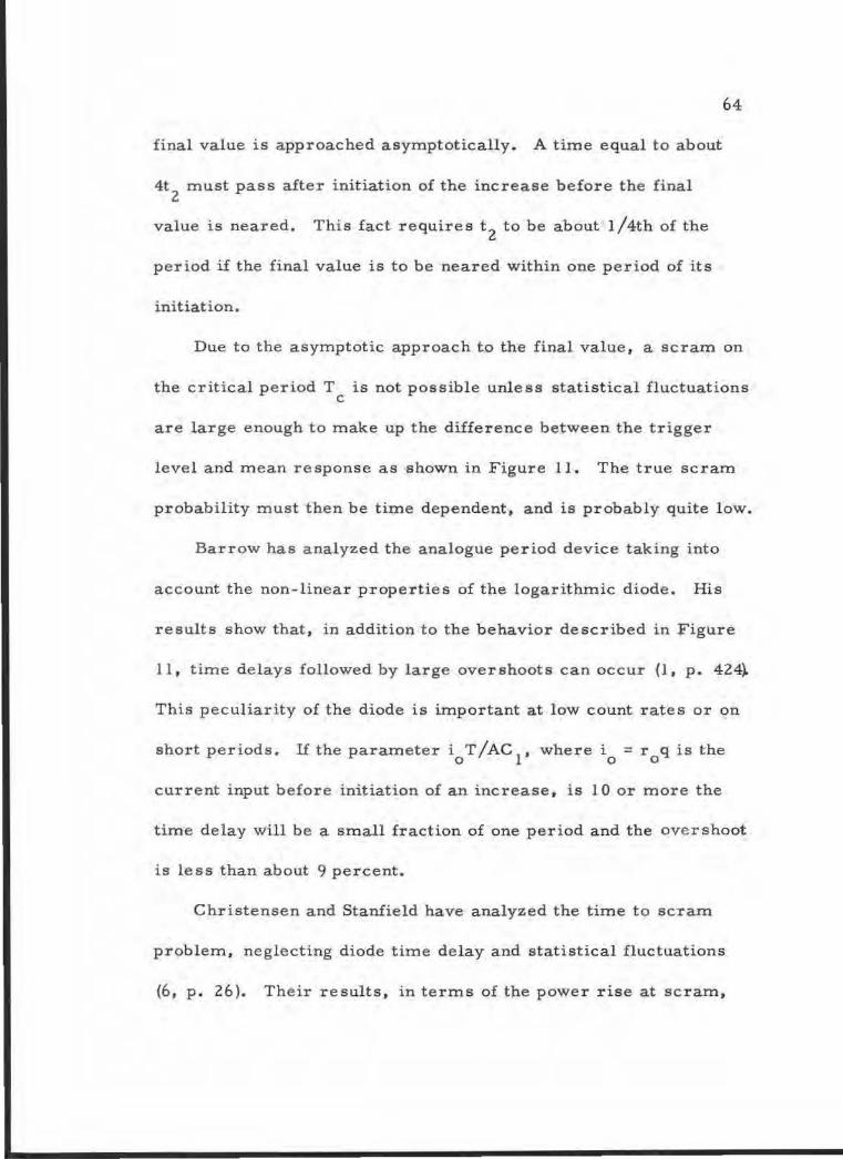
optimum value of the ratio t t is unity (1 p 423 ) The transhy3 2
sient response for this case is plotted in Figure 11 Note that the
10
63
0 8
0 6
Transient Response of Typical Analogue Period Device Having
0 4 = t Neglecting Diode Timet 2 3
Delay
02
0
0 1 2 3 4 5 6 7 8 9
Time Normalized tt2
Figure 11 Transient Response of Analogue Period Meter
2
64
final value is approached asymptotically A time equal to about
4t must pass after initiation of the increase before the final
value is neared This fact requires t to be about l4th of the2
period if the final value is to be neared within one period of its
initiation
Due to the asymptotic approach to the final value a scram on
the critical period T is not possible unless statistical fluctuations c
are large enough to make up the difference between the trigger
level and mean response as middotshown in Figure 11 The true scram
probability must then be time dependent and is probably quite low
Barrow has analyzed the analogue period device taking into
account the non-linear properties of the logarithmic diode His
results show that i n addition to the behavior described in Figure
11 time delays followed by large overshoots can occur (1 p 424~
This peculiarity of the diode is important at low count rates or on
short periods If the parameter i T AC where i = r q is the 0 1 0 0
current input before initiation of an increase is 10 or more the
time delay will be a small fraction of one period and the overshoot
is less than about 9 percent
Christensen and Stanfield have analyzed the time to scram
problem neglecting diode time delay and statistical fluctuations
(6 p 26) Their results in terms of the power rise at scram
65
are useful since the solution of equation 34 or 35 for t given e (t)3
must be obtained graphically If t t is unity or larger their 3 2
results show that one period scrams are possible only over a narshy
row range of period less than one decade when t is about T 4 2 c
The minimum possible time to scram is t and reducing it 2
widens the period range over which one period scrams are posshy
sible Statistical fluctuations limit t 2 to some minimum value
however A narrow range of one period scrams with large power
increases before scram on periods slightly less than Tc and very
large power increases on very short periods is the general patshy
tern
In addition to the finite range of period where one period
scrams are possible and the difficulty of obtaining scrams on par shy
iods equal to T the analogue device offers little protection c
against short accident periods Diode time delay at short perishy
ods further increases the short period scram time An example
device described by Christensen and Stanfield having a t of 8 2
seconds allows the power to rise by a factor of 4 7 x 1o4 before
scram is inititated on a period of 0 01 seconds (6 p 25
The dynamic behavior of a given device can be readily anshy
alyzed with the aid of the cited references but no synthesis proshy
cedure has been developed Examples presented by Barrow are
66
perhaps definitive of the capabilities of analogue period devices
A device having t 2 =t 3 = 4 seconds approaches within 10 percent
of the final value in 90 seconds when the period is 15 seconds and
in 14 seconds when the period is 3 seconds There was no overshy
shoot on the 3 second period but an overshoot to a 12 second pershy
iod indication at 25 seconds occurred on the 15 second period
Barrow considers these figures as bullbull bullbullbull considerable improvement
over period meters built previouslybullbull (2 p 366)
Statistical Fluctuations
The need to keep false scrams from occurring more than a
tolerable amount places limits upon the minimum time constants
of an analogue period device Thus the transient response is
limited by the threat of excessive statistical fluctuations
Shot noise consists of impulses having a fixed magnitude but a
Poisson distribution in time Treatment of the statistical fluctuashy
tions in analogue devices begins by assuming that shot noise is
present in the diode current The varian ce of the diode voltage
is then found to have a magnitude independent of count rate with
a frequency spectrum proportional to count rate (6 p 23 1 p
425 ) The result expressing the variance of the diode voltage is
equation 36
67 2
36 0D = 1r AqZC I
Christensen and Stanfield obtain the ratio of the variance of
2 1the output voltage to ODmiddot as a function of t t and t t bull If no
3 2 2 1
filter network is present the variance ratio ls very small at low
count rates and rises smoothly to unity at about t t = 100 The2 1
output variance is half the diode variance at about t ti of unity 2
With a filte r network the ratio rises to a maximum at t 2tt~ t t bull 2 3
The peak magnitude of the ratio for t =t is 0 125 while one 2 3
count decade above and below the peak the ratio is 0 0413
Barrows conclusion that the optimum ratio of t t is unity3 2
results from the fact that the fastest response for a given reducshy
tion in output noise power is achieved when t = t (l p 42 3 ) 2 3
The per unit deviation at the output is a function of time
period device parameters and count rate If diode time de lay
and overshoot are neglected the steady state per unit deviation
can be plotted This is done for a 1 0 second period in Figure 12
for three typical devices whose parameters are consistent with
those of published examples The per unit deviation is converted
to accuracy at a 0 9974 reliability to allow comparison with other
1 The ratio t t is proportional to count rate since t is the
2 1effective time cohstant of the logarithmic network t =AC rq
1 So t 2tL =qrt2 AC bull The diode is assumed to be linear for1
1small cbanges in current so its resistance is dedi
gt
-I ~ -I
Q)
~ gt=
1~ 10 l)
~ ~ (x5) cU 1-lt 1 u u lt (x2)
10deg 2 10
1-Typical Analo 1 2 1Typical[Analo 2 3 J Typical fAnalo C se 4 Near Op~imum Digita At T =1 1 5 1Near Opltimum Digita tltT = 2
(x2) (x5) 1 0
--------~-----~----~~------~----middot
Count Rate at Time of Indication Per Minute
Figure 12 Steady State Accuracy of Analogue Period Meter
69
plots in this paper Accuracy values are inversely proportional
to the output voltag~ Time dependent values can be obtained by
dividing the ordinates in Figure 12 by the ratio of instantaneous
to steady state output voltage Similarly accuracy values for
periods T other than l 0 seconds are found by multiplying the
ordinates by T 10
In all cases presented in Figure 12 A 0 1 volts per neper
C 1 = ljJf and t 2 =t 3 bull Cases 1 and 2 have t 2
= 2 5 seconds while
= 5 seconds in case 3 Values of charge q are 1 o- 9 coulombst 2
in cases 2 and 3 and 5 x 10- 9 coulombs in case 1
Smaller t 2 values will shift the curves of Figure 12 upward
and to the right All other parameters staying constant the neeshy
essary accuracy at a given count rate determines the minimum
acceptable t The compromise between accuracy and speed of2
response is unavoidable in an analogue period device
Shown also in Figure 12 are accuracy curves for digital reshy
ciprocal period measuring devices The total digital measureshy
ment time t is equal to 4t and the count rate is that at time t2
instead of the initial value Counting times are set to give the
ultimate accuracy as determined from Table 2 Extension to
periods other than 10 seconds requires recalculation since tT
changes horizontal as well as vertical shift of the digital curves
70
results
The ultimate digital device has superior accuracy at higher
count rates The magnitude of this superiority is a function of
period but it does not appear to be great at any period Accuracy
superiority of the analogue device at lower count rates may not be
realized due to the large accuracy values at lower count rates A
digital device affords a slight accuracy superiority over an anashy
logue device in general
It must be emphasized that the analogue accuracy values
shown in Figure 12 are achieved only in the steady state At a
time equal to 4t2 after initiation of an increase Figure 11
shows the true ordinates to be l l times those plotted in Figure 12
COMPARISON OF ANALOGUE AND DIGITAL PERIOD DEVICES
Figure 12 shows the s teady state accuracy of an analogue
reciprocal period measurement to be nearly that predicted by
statistical fluctuations at higher count rates and actually superior
at lower count rates Transient response as shown by Figure ll
sets the practical limitation on the use of analogue period measur shy
ing devices
The main advantage to be gained by the use of a digital period
measurement is freedom from transient response limitations
71
Accuracy can be specified independent of time along with the true
and false scram probabilities Knowledge of the ratio of instantashy
neous to steady state output voltage is not required to specify
instantaneous accuracy of an analogue device On a dynamic or
instantaneous basis the accuracy of a digital device can be subshy
stantially bette r than that of an analogue device
A digital mechanization of the weighted increase function is
significantly better than an anal ogue device from the standpoint of
providing reliable warning of dangerou s periods One period
scrams can occur with a specified probability for periods ranging
from the counting time to the critical value A wide period range
digital system will not provide the ultimate accuracy but is much
more dependable than an analogue device The most accurate digshy
ital system will probably give one period scrams over a wider
range than an analogue device Figure 8 ~gthows that the weighted
increase function can provide a significant accuracy advantage if
the comparison time is not too long
ln contrast to the dependability of a digital period scram
device on periods equal to the critical value the true scram
probability of an analogue device is very small on the critical
period For an analogue device having a steady state accuracy of
about 10 percent the true scram probability at a time 4t after 2
72
initiation of the critical period is about 0 001 This probability
approaches 0 50 as the output voltage reaches its final value An
acceptable steady state false scram probability does not mean that
an excessive number of false scrams can not occur with an anashy
logue device due to the possibility of poor dynamic accuracy
CONCLUDING COMMENTS
The object of this paper was to investigate the limitations imshy
posed by statistical fluctuations in nuclear reactors on measureshy
ments of reactor period Figures 8 and 12 summarized thereshy
sults The analyses used were approximate but sufficiently acshy
curate to investigate the feasibility of digital period measuring
devices A compute r is required to make extensive investigashy
tions of the more exact relationships Experimental evidence was
presented to justify the assumption that the statistical fluctuations
present in nuclear reactors follow a Poisson distribution The
methods of analysis used do not depend upon this assumption and
the results obtained could be modified for other statistical
distributions
A digital approach to measurement of reactor period and
generation of dangerous period indications is feasible from the
standpoint of performance Digital mechanization would be
73
expensive however The coming application of digital computers
to the middot control of nuclear power plants may make digital mechanishy
zation feasible from an economic standpoint Period measuring
functions would share the control computer with other reactor
control functions
It was not the purpose of this paper to suggest a specific
digital mechanization or to determine minimum performance
standards Preliminary investigation of a fixed count adaptive
approach to digital measurement of reciprocal period shows sufshy
ficient promise to merit mention however This approach in-
valves comparing the results of successive count rate measureshy
ments to determine reciprocal period as does any digital ap shy
preach but with the counting times varied to make the counts
occurring in each counting interval constant A computer is
needed to e xtensively investigate the equation describing this apshy
preach Preliminary hand calculations show the accuracy
function to have a sharp null as a function of (t + t )T with c 1 c2
the magnitude at the null a factor of ten smaller than that predic shy
ted by Figure 4 for the situation investigated An adaptive system
is necessary to maintain the operating point at the null over a
wide range of operation Adaptive digital control of process
plants is relatively new but we might reasonably expect the art to
advance to where this type of control is useful with nuclear reactors
7 4
BIBLIOGRAPHY
1 Barrow Bruce B The logarithmic diode counting rate meter and period meter Transactions of the American Institute of Electrical Enginee-rs Part I - Communication and Electronics 7 6421-427 1 957
2 Barrow Bruce B and Robert Maitland Transients in logshyarithmic count rate and period meters Transactions of the American Institute of Electrical Engineers Part I shyCommunication and Electronics 79362-369 1960
3 Bartlett MS An introduction to stochastic processes Cambridge University Press 1955 312 p
4 Biehl A T et al (eds ) Elementary reactor experimentation San Ramon Cal Aerojet-General Nucleonics 1957 189 p
5 Chemical Rubber Publishing Company Standard mathematical tables lith ed Cleveland 1957 480 p
6 Christensen Helge and Robert B Stanfield The log count rate period meter used with safety circuits IRE Transshyactions on Nuclear Science NS - 822-26 July 1 961
7 Courant E D and PR Wallace Fluctuations of the number of neutrons in a pile Physical Review 721038-1048 1947
8 Crow Edwin L Frances A Davis and Margaret W Maxfield Statistics manual New York Dover 1960 288 p
9 de Hoffman Frederic Statistical aspects of pile theory In Clark Goodmanbull s ed) The science and engineering of nuclear power Vol II Philadelphia Addison- Wesley 1949 p 103-119
10 Diven B C et al Multiplicities of fission neutrons Physical Review 1011012-1015 1956
75
11 Grim William M Jr Bruce B Barrow and John C Simons Jr Random fluctuations in period meter indications Nuclear Science and Engineering 180-91 1956
12 Handloser John S Health physics instrumentation New York Pergamon Press 1959 182 p
13 Harris D R Analysis of reactor fluctuations Transactions of the American Nuclear Society 4317-318 1961
14 Harris D R Stochastic fluctuations in a power reactor Pittsburgh Westinghouse Electric Co 1958 37 p (US Atomic Energy Commission WAPD-TM-190)
15 Harvey Roland A The selection of optimum time constants for RC filters with random signals IRE Transactions on Nuclear Science NS - 985-90 April 1962
16 Hoehn Gus L Jr Semiconductor comparator circuits IRE WESCON Convention Record 3(2)101-110 1959
17 Hurwitz H Jr et a l Effects of neutron fluctuations on reactor operations Transactions of the American Nuclear Society 3 477 1960
18 Jordan W H H B Frey and G Kelley An instrument for measuring the logarithm of neutron level and the period of a pile Oak Ridge Tenn National Laboratory 1948 13 p (ORNL- 110)
19 K eepin G R and T F Wimett Reactor kinetic equations a new evaluation Nucleonics 1686-90 Oct 1958
20 Lehr Samuel N and Vernon P Mathis A digital start up control for air cooled nuclear reactors Transactions of the American Institute of Electrical Engineers Part I shyCommunications and Electronics 7 9369-37 5 1960
21 Molina E C Poissons exponential binomial limit Princeton NJ Van Nostrand 1942 47 p
22 Mori Hideo and Eugene P Johnson Jr Basic statistical theory In William W Seifert and Carl W Steeg Jr s (eds) Control systems engineering New York McGrawshyHill 1960 p 406 - 541
76
23 Motorola Inc Reliability and Components Group Reliability and components handbook Phoenix Ariz rev 1959 6 sections
24 Murray Raymond L Nuclear reactor physics Englewood Cliffs N J Prentice-Hall 1957 317 p
25 Pearson Karl Tables for statisticians and biometricians Part I 3d ed 143 p
26 Price William J McGraw- Hill
27 Rand Corporation
Cambridge University Press 1930
Nuclear radiation detection New York 1958 382 p
A million random digits Glencoe Ill Free Press 1955 200 p
28 Toppe1 B J Sources of error in reactivity determinations by means of asymptotic period measurements Nuclear Science and Engineering 5 88-98 1960
2 9 Vincent C H The rapid recognition of a significant increase in the rate of arrival of pulses occurring at random Nuclear Instruments and Methods 9181-194 1960
30 Wade E J and D S Davidson Transistorized log-period amplifier IRE Transactions on Nuclear Science NS- 653 shy56 June 1959
31 Wadsworth George P and Joseph G Bryan Introduction to probability and random variables New York McGrawshyHill 1960 292p
APPROVED
----~-
Associate Professor of Electrical Engineering
In Charge of Major
Chairman of School Graduate Committee
Date thesis is pre s e nte d_--=gtE=--(~_1_middot_zmiddot_plusmnL_~I_1~0-=_____
Typed by Carol Baker
ACKNOWLEDGMENT
My special thanks go to Associate Professor Robert R
Michael for his helpful suggestions and encouragement during
the research for this paper The efforts of Assistant Professor
Edward A Daly made the reactor experiment possibl e
TABLE OF CONTENTS
Page INTRODUCTION l
INTRODUCTION TO REACTOR MEASUREMENTS 2
Basic Concepts 2 Reactor Kinetics 4
NUCLEAR REACTOR FLUCTUATIONS 7
Statistical Terms 8 Nature of the Fluctuati ons 10 Radioactive Decay Statistics 11
EXPERIMENTAL DETERMINATION OF REACTOR FLUCTUATION DISTRIBUTION 13
Simple Power Measurement 21 Reciprocal Period Measurement 30 Operating Parameters 35 Quasi-continuous Measurement 36
GENERATION OF RELIABLE PER IOD SCRAM 41
Basic Increase Function 41 Optimum Increase Function 44 Weighted Increase Function 47 Comparison of Measurement Types 50 Design of Optimum Period Scram Device 51 Maximum Acceptable Accuracy Values 52 Quasi -continuous Measurement 56
COMPARISON OF ANALOGUE AND DIGITAL PERIOD DEVICES 70
CONCLUDING COMMENTS 72
BIBLIOGRAPHY 74
LIST OF TABLES AND FIGURES
Table Page
1 Reactor Test Results 15 2 Per Unit Deviation of Reciprocal Period
Measurement 40
Figure 1 Accuracy of Count Rate Measurement 26 2 Accuracy of Count Rate Measurement 29 3 Reciprocal Period Indication Ratio 32 4 Accuracy of Reciprocal Period Measurement 34 5 Accuracy of Reciprocal Period Measurement
as a Function of Counting Time 38 6 Accuracy of Basic Increase Function
Measurement 43 7 Magnitude of Vincent s Optimum Increase
Function 46 8 Accuracy of Weighted Increase Function
Measurement 49 9 Illustration of Accuracy Parameter 54
10 Typical Analogue Period Meter 61 J 1 Transient Response of Analogue Period Meter 63 12 Steady State Accuracy of Analogue Period Meter 68
ANALYSIS OF NUCLEAR REACTOR PERIOD MEASUREMENTS
The production of power in a nuclear reactor involves complex1
dynamic processes which require censtant observation to assure
safe efficient utilizat ion These observations consist of measure shy
ments to determine such thing s as power levels control rod posishy
tiona temperatures and others depending upon the size and comshy
plexity of the reactor The statistical nature of the processes in-
valved complicates these measurements This paper is concerned
with one type of measurement that which determines the rate of
change of reactor power
The time rate of change of power is usually expressed in terms
of the period of the reactor This is the time taken for the power
to change by a factor e (the base of natural logarithms) Assuming
the reactor response to be exponential the reciprocal of the period
is the coefficient of time in t he e xponent of e Careful control of
the period is necessary particularly on start up to prevent rapid
power increases It is essential for reasons of safety that the reshy
actor not be allowed to become critical with prompt neutrons alone
Monitoring the period is an effective way to prevent this
Common period measuring systems are analogue devices whose
performance is limited by factors inherent in the devices themshy
selves and by statistical fluctuations Direct comparison of the
2
performance of an analogue device with that dictated by statistical
limitations has not been published Once this comparison is made
the feasibility of a digital device can be determined The object of
this paper is to make this comparison
INTRODUCTION TO REACTOR M EASUREMENTS
Some knowledge of the behavior of a nuclear reactor is required
before one can attempt to analyze devices used for reactor measureshy
ments It is not intended that a lengthy description of reactor
physics and kinetics be given here standard textbooks and referenshy
ces are to be consulted
Basic Concepts
A nuclear reactor might be de scribed as a system for controlshy
ling a neutron chain reaction Neutrons created during the fission
of certain heavy nuclei survive to initiate fission in other heavy
nuclei When the ratio between the number of neutrons created in
one generation and those created in the generation immediately preshy
ceding is exactly unity the reaction is self sustaining This ratio is
called the effective multiplication factor K e
Each fission event releases energy which is distributed among
fission fragments neutrons neutrinos and decay gamma rays beta
particles and alpha particles A total of about 201 Mev is released
3
in the fission of uranium 235 of which about 190 Mev can be
1 d 1 If a filtCed amount of energy per fission is made availableuhtze
and transferred to the reactor as heat power the power level is
directly related to the fission rate The exact correlation depends
upon the degree of equilibrium between fission product production
and decay and upon the fraction of gamma rays which escape from
the reactor (24 p 5 )
It will be assumed that reactor power is directly proportional
to the fission rate This is a basic assumption upon which importshy
ant nuclear measurement techniques are based Thus the reactor
2power can be found by determining the fission rate
The neutrons in a reactor are distributed throughout the core
with a distribution of energy and direction A convenient quantity
in this regard is the neutron flux ~ with the units neutrons per
square centimeter per second This is the ratio between the reacshy
tion rate per unit volume and the macroscopic cross section 24 p
23 )
The fission rate may then be determined by measuring the flux
This is frequently done using a detector filled with a suitable gas
1 The neutrinos carry about 11 Mev from the system
2 Murray states that 3 3 x 1o1 0 fissions of uranium 235 per second are necessary for the production of 1 watt of reactor power (24 p 5 )
4
Neutrons passing through the detecter collide with constituents of
the gas creating ionizing particles The ions and electrons created
by these secondary particles are rapidly swept to electrodes by a
strong electric field A voltage pulse at the detector output is the
result The number of pulses per unit time is proportional to the
flux at the detector location Another type the ion chamber gives
a current output proportional to the flux These devices are
descr ibed in the book by Price (26 chapter 9)
It is assumed when making neutron flux measurements that
the d e tec tor output is directly proportional to the reactor power
This means that the flux at the detector location usually a region of
relative ly low flux near the core periphery is representative of the
high core flux It is a problem for the reactor designer to select
detector locations where the assumption of proportionality between
detector output and reactor power is valid Spatial flu~ distribushy
tions in the reactor may require the use of several detectors whose
outputs are combined in some manner to give the reactor power
Reactor Kinetics
As the power level detector is triggered by neutrons it is desirshy
able to hav e some knowledge of the time behavior of neutron flux
A pair of equations developed from a space independent model
which considers only one neutron energy group are commonly used
5
to determine the neutron density 19 p 86) An average flux is
then obtained by multiplying this density value by the mean velocity
of the group considered These equations are
6
1 dndt = (eKe - (3Ke)nL + I Xiyici and
i=l
2 de dt = 3 K nL - X c 1 1 e 1 1
In equations 1 and 2
n is the neutron density
Cmiddot1 is the density of the ith precursor
K is the effective multiplication factor e
oKe is the
L is the prompt neutron lifetime
is the fraction of neutrons due to the ithl3i precursor
3 is the total de layed neutron fraction
x_ 1 is the decay constant of the ith precursor
y is the effectiveness of ith precursor neutrons1
in producing fission as compared to prompt neutrons
If an artificial fast neutron source is present sf is added to equashyf
tion 1 with S being the source strength and f the fraction of source
6
neutrons which do not escape from the system (24 p 166)
The kinetic equations can be solved by assuming an exponential
character for n and c Substituting into the original equations1
yields the seventh order inhour equation with T as the variable J
6 3 oK K = LKeTJ + Yf3 j( 1 + gt middotT )e e Ltl lJ
i~l
1The solution of equation 3 when S = 0 is (24 p 156-159)
7
4 n =A exp (tT )L J J
j= 1
lf the reactor is not critical all roots T of the inhour equationJ
are negative If the reactor is super-critical one root is positive
The other six arising from the existence of delayed neutrons are
negative Transient behavior with a step change in reactivity is not
a single exponential function but a composite of seven exponential
terms The period of super-critical reactor is approached asympshy
totically as the negative exponential terms decay The asymptotic
period is the positive root of the inhour equation For a sub-
critical reactor the negative period approached is the largest negashy
tive root of the inhour equation provided S equals 0
1 Murray reference 24 considers only five groups of delayed
neutrons More recent information by Keepin reference 19 conshysiders six groups Murrays equation is modified by this fact to give the same result as Keepin
7
The assumption that a single exponential function is a good
approximation to the complete solution of the inhour equation is
implicit in period measuring devices Toppel has calculated the
time required after a step change in reactivity for the difference
between the asymptotic reciprocal period obtained from the inhour
equation and the value obtained from the single exponential approxishy
mation to become less than a specified fraction of the asymptotic
value (28) This waiting time can be as long as one period in a
source free reactor when the asymptotic period is about 10 seconds
or less (28 p 91 and longer in reactors containing sources (28
p 96) Discussion of the effect of the single exponential approxishy
mation on period measuring devices is beyond the scope of this
paper It will be assumed that this approximation is sufficiently
valid to permit useful period measurements to be made
NUCLEAR REACTOR FLUCTUATIONS
A moment 1 s consideration will show that even in a reactor
operating at a steady power level the neutron flux must fluctuate
with time The various processes by which neutrons interact with
nuclei are described by cross sections (24 p 20) Cross sections
are a measure of the probability of occurrence for a given reaction
and their magnitude is a function of neutron energy Fission
8
neutrons are not created with a fixed energy but with a distribution
of energy (24 p 38) Likewise thermalized neutrons do not have a
fixed energy (24 p 30) A fixed number of neutrons is not created
in a fission (1 0 ) one must consider the probability that a given numshy
ber are created The number of collisions with moderator nuclei
required to thermalize fission neutrons is not a constant but will
vary from one neutron to another due to variations in the scattering
angle (24 p 37 )
The energy of neutrons in a reactor varies over a large range
with a certain probability for a given number lying in a given range
The various processes occurring within the reactor must be deshy
scribed by energy dependent probabilities Because of these facts
average values are used when reactor behavior is discussed Mean
thermal neutron energy mean fission neutron energy mean neushy
tron lifetime and mean number of collisions to thermalize are
terms frequently used
Statistical Terms
In this paper we are interested in the nature of the neutron flux
fluctuations Before discussing this further it would be well to de shy
fine several statistical terms which will be encountered frequently
It must be recognized at the outset that the shape of the curves
showing the results of experiments performed on statistical
9
processes need not be the same Several types of statistical proshy
cesses have been mathematically described in terms of the form of
the experimental results
The basic mathematical description is the probability density
function p(x) (22 p 419-421) To find the probability of obtaining
a result within certain limits p (x) is integrated between those limshy
its This density function is normalized to make the area u nder its
curve unity The variabl e x may be discrete or continuous depend shy
ing upon the process i n question
The probability distribution function P (x) is the integral of the
density function p (x) from negative infi nity to x It expresses the
probability of obtaining a result less than x (22 p 428)
SX
5 P (x) ~ p (x )dx
-00
The familiar normal distribution is an example (22 p 439)
1 2 6 P (x) = (1CJ~) exp - (x- M )
za2
Values of the normal and other distribution functions are tabulated
(5 8 21 25)
Of special1nterest are the average properties of the process
These are found from the moment functions of mth order (22 p
456)
10
S00
7 Mm (x) = xmp (x)dx
-00
The moment function gives the expected value of xm For example
the first moment (m equals one) is the mean and the second moment
is the mean square of the process
2 The variance ltY a common measure of the spread of a distri shy
bution is the second central moment Central moments are obshy
tained by biasing ordinary moments by the mean of the distribution
(22 bull p 4 57 ) bull
00
8 C m (x) = S[x - M 1 (x)Jm p (x) dx
-00
It can be shown that the variance is the difference between the mean
square and the mean squared (22 p 459)
2 1 29 ()2 (x) = M (x)- [M (x) ]
Nature of the Fluctuations
The information of interest here is the type of distribution folshy
lowed by the reactor fluctuations Some theoretical trea tment has
been given to reactor fluctuations in the literature (7 9 13 14
17 ) Two papers present a thorough theoretical treatment considshy
ering a sub-critical reactor as a stationary random process (7 14)
11
The term stationary refers to a process whose statistical charactershy
istics are not time dependent (22 p 417) The term random reshy
fers to a physical process containing a random element (3 p 1 )
The mathematical techniques used are in the realm of advanced
mathematical statistics and will not be considered here However
the assumption that the process is random and stationary seems unshy
duly restrictive Harris (14 p 30) feels that a critical reactor
will not be a random process and that in any case the counting sys shy
tem c a n n ot be stationary Clark 1 feels that a reactor is a Markov
rather than a random process The methods used with Markov proshy
cesses account for a lack of statistical independence in the system
studied In a reactor the neutron flux at any given time is related
to the flux extsting earlier and some statistical dependence must
be present
Radioactive Decay Statistics
With the lack of a theoretical result suitable for engineering
purposes it was necessary to develop a model which would lead to
a readily applicable result The first one which comes to mmd is
the decay of radioactive nuclei
The stati stics of radioactive decay are discussed by Price (26
1
Mr R G Clark Hanford Atomic Works private communication
12
p 53-56) He states that the distribution followed is the binomial
distribution (26 p 55) If the number of nuclei decaying in a given
time interval is much less than the total number present at the
start of the interval and if the product of the decay constant and
time interval is much less than unity the simpler Poisson distrishy
bution is an excellent approximation Decay statistics are comshy
monly assumed to follow the Poisson rather than the binomial
distribution
The Poisson distribution is characterized by the following
probability density function (31 p 67 )
u X
exp (-u)10 p (x) = x
In equation 10 xis a discrete variable Calculation of the first
and second moments shows that the mean and variance of the distrishy
bution are both equal to u (31 p 203 )
The assumption that a process follows a Poisson distribution
is very convenient Only one parameter u is required to comshy
pletely describe the process No separate calculation to find the
variance is necessary
13
EXPERIMENTAL DETERMINATION OF REACTOR FLUCTUATION D1STRIBUTION
An experiment to test the validity of assuming that a reactors
fluctuations follow a Poisson distribution was performed The re shy
actor at Oregon State University an Aerojet-General Nucleonics
AGN 201 was used This is a low power reactor designed for trainshy
ing purposes The lack of a general theory for reactor fluctuations
applicable to a critical reactor made experimentation necessary
Experimental Methods
The equipment and procedures used were essentially routine
A boron-trifluoride filled thermal neutron detector Radiation
Counter Laboratories model 10502 was installed in one of the reshy
actor loading ports The flux at the detector location was the order
of a hundredth of the maximum core flux (4 p 165 )1 Mechanically
coupled to the detector was a cathode follower circuit providing a
low output impedance to eight feet of coaxial cable transmitting de-
teeter pulses to Tracerlab RLI-1 linear amplifier A Hewlett-
Packard 524C electronic counter gave the output information
The detector was relatively insensitive to gamma rays A
The sensitive volume of the detector was located outside the graphite reflector and most of the lead shield The flux varies with distance from the center of the core so the detector output represhysents a spatial average
14
radium source placed adjacent to the detector resulted in the obsershy
vation of pulses no larger than 5 millivolts Using the shut down
reactor as a source of neutrons resulted in the observation of pulses
up to 60 millivolts In a high mtensity gamma ray field the small
pulses due to individual gamma rays can pile up to produce brger
pulses which can not be distinguished from those due to neutrons
(the neutron detector was used as a proportional counter j The deshy
tector was placed in the loading port with the reactor operating at
full rated power and a curve of count rate as a function of detector
voltage was obtained This curve showed a plateau of about 400
volts length with a slope of about l 25 percent per l 00 volts The
presence of this wide plateau is evidence that the gamma ray field
was not sufficiently intense to produce pile up effects (12 p 88)
Experimental Results
The results of this experiment and associated calculations are
shown in Table l Sarnple mean and sample variance characterize
the raw data The latter consists of a number of readings of counts
accumulated during a flxed time interval This was conveniently
done with the Hewlett-Packard 524C counter which would count for
a pre set interval hold the result for a fixed time then automatically
reset and resume cotAnting In all cases the reactor was as near a
condition of equilibrium as was possible to achieve
15
Table 1 Reactor Test Results
Nominal Counting Sample Sampl e Sample Sample Power Time Size Mean Variance_____________________________________________
1 1 mw 10 sec 25 128476 402552
2 1 100 13669 43016 3 II 0 I 100 13 13 2838
4 It 0 01 so 1 74 1 83
5 10 mw 10 25 987452 5567934
6 II 1 100 82570 1171 38
7 It 10 10 842690 1396121
8 II o 1 100 83 15 98 43
9 0 1 100 101 46 97255
10 II o 01 50 834 862
11 100 mw l 100 845056 1381221
12 II 1 24 811779 755956
13 0 l 25 85 7 12 69128 14 It 0 01 25 8564 5824
15 II o 01 100 8550 78 88
16 II 0 1 100 844 82 733 48
----------------------------------------------
16
1
Table 1 (Continued)
Data 2 2Sample Intervals Sample X Critical X
1 4 6 66 40 29
2 8 7771 124 12
3 7 6976 124 12
4 4 10 97 6369
5 2 0 04 41 64
6 11 1185 124 12
7 2 0554 18 48
8 7 1o 69 124 12
9 4 133 1 12 4 12
1o 6 938 6369
11 7 1280 124 12
12 4 0 7 01 40 29
13 3 0 356 4029
14 4 1 61 4164
15 12 888 12412
1 6 9 7 95 124 12
Critic al values taken at 1 percent significance level (8 p 232) 1
17
The sample mean is an unbiased estimate of the population mean
and is calculated by dividing the sum total of all counts in the samshy
ple by the sample size (number of successive readings) Taking the
mean of all possible unbiased estimates of a given parameter yields
the parameter in question (31 p 206 Likewise the sample varishy
ance s 2
is an unbiased estimate of the population variance cr 2 bull This
is calculated from (8 p 13)
11 --1 -- n x
1n(n - 1) L
In equation 11 n is the sample size and x is a member of the samshyi
1ple
Analysis of Results
The problem of determining what distribution is followed by a
set of raw data is that of fitting a curve to the data One approach
is to group the data in sufficiently small intervals and plot the number
in each intervalas a function of the variable the plot being similar to a
vertical bar graph Then a distribution is assumed andplotted on the
same axes Ifthe assumed curve closely follows the actual results the
distribution assumption is valid It is 9-otpossibl~ however to state the
degree of validity This is a subjective rather than object~ve method
The mean of all possible second central moments yields not o-2 but (n- 1)nx o-2 (31 p 206)
1
18
Statisticians have developed an objective method the chi-
squared (X 2 ) test (8 p 83-88 31 p 238-242) This involves
calculating the X 2 statistic for each sample and comparing it with
tabulated values at a stated significance level If the sample x 2 is less
than the tabulated X 2 the assumption is considered valid The statisshy
2tic X compares the actual and assumed relative frequencies (occurshy
rences per interval compared to total occurrences)
2The X statistic with r - 1 - g degrees of freedom is found from
the following relationship (8 p 85 )
r 2 - ei)
12 x2 =I (nishy
e 1
i=l
In equation 12 ni is the actual number of occurrences in the ith inshy
terval ei is the assumed number of occurrences g is the number
of assumed distribution paramete r s based upon the data and r is
the number of intervals
The sensitiveness of this test de)ends upon the number of
intervals r If a small enough number of intervals is used almost
any assumption will pass the test On the other hand if r is so
large that the assumed number of occurrences per interval is very
2small unrealistically large X values result There is no way to
explicitly surmount these difficulties However both references
consulted are agreed that the minimum number of assumed
19
occurrences per interval should be five
The sigmficance level sets the likelihood that a true assumption
will be rejected (8 p 16 ) For example if a 1 percent significance
level is chosen a true assumption will be accepted in 99 percent of
the tests on the average
Values of x2 were calculated for each sample assuming a
Poisson distribution with a mean equal to the sample mean These
values are compared to the critical values taken from the table (8
p 232) at the 1 percent significance level The table contains valshy
ues only for 100 degrees of freedom (df or less taken i n intervals
of 10 past 30 The df for most samples fell between tabulated valshy
ues When that was the case the next lowest tabulated value was
used This gave pessimistic values for the critical X 2 values
The Poisson table used to find the expected number of occurshy
rences per interval considered mean values only to l 00 If the
sample mean was less than 100 the assumed Poisson mean was the
nearest integer (but for sample 4 where 1 70 was assumed) to it
When the sample mean was greater than 100 a normal distribution
with mean and variance equal to the sample m ean was assumed
The Poisson distribution can be approximated by a normal disshy
tribution if the mean is sufficiently large Price considers a mean
of 100 or greater sufficient to make the normal approximation to the
20
Poisson distribution valid (26 p 57) Since the normal distribution
is more thoroughly tabulated than the Poisson distribution this
approximation is often convenient
The raw data and chi- squared test calculations are too lengthy
to include in the paper
Conclusion
The assumption of a Poisson distribution or an approximate
normal distribution for nuclear counting fluctuations is both convenshy
ient and widespread Table l shows the results of the chi- squared
test performed upon reactor counting data with this assumption All
samples but one number 9 pass the test This indicates that the
Poisson distribution assumption is valid within the meaning of the
chi-squared test Table 1 does not indicate that a Poisson distribushy
tion is the only or even the most accurate assumption Even with
an objective test judgement must be used in reaching a final conshy
number of intervals relation between sample and critical chi shy
squared values experimental methods and perhaps others
For example consider the very small X 2 values obtained in
samples 5 7 and 13 Only two or three intervals were possible
with the small sample size These results should not be given the
same weight as the larger but still relatively small X 2 values in
21
samples 15 and 16 On the other hand the large x 2 value of sample
9 might be discounted as the one in a hundred which gives a negative
result with a true assumption The only difference between samples
8 and 9 is the linear amplifier gain (more small pulses are counted
in sample 9) and sample 8 has a relatively small X 2 value
On the basis of the results shown in Table 1 nuclear reactor
fluctuations as seen by counting device will be assumed to follow a
Poisson distribution in this paper
STATISTICAL LIMITATIONS UPON MEASUREMENT
Consecutive measurements made during a finite time interval
of some property of a statistical process will rarely be identical
This is a direct result of the fact that the property in question
1fluctuates about some mean value The measured fluctuation will
be relatively smaller than the instantaneous process fluctuations due
to averaging inherent in the finite time interval measurement To
reduce relative fluctuations a longer time interval (larger sample
size) must be used
Simple Power Measurement
The count rate of a pulse type neutron detector is proportional
1 The independent variable is not necessarily time but iq this
paper it is the only one considered
22
to reactor power if the detector is properly located Ipound a mean
count rate r exists the fluctuations in the count rate are
J 3 () 2 = t
r c
when the fluctuations follow a Poisson distribution (26 p 59)
Note that the fluctuations exist in the number of events n = rt that c
occur during the time interval t rather than in the events per unit c
time r
The variance in the number of counts per interval n may be
equal to n only when the count rate is constant during the counting
inter val Price shows that this variance is n exp (- t ) for radioshyc
active decay when the counting time tc is not small enough to make
tc lt lt 1 (26 p 56) In an analogous manner equation 13 is mulshy
tiplied by exp (tcT) when tc is not much smaller than the period T
of an exponential increase
Equation 13 for the count rate variance neglects any fluctua shy
tions in the counting time t which must exist with any physicalc
measuring device In order to determine how the counting time
fluctuations affect the result the rule for combining vanances in
an equation containing fluctuating quantities must be known The
answer is provided by the Motorola handbook (23 section 3 2 4
p 5 ) Ipound y is a function of x X x then the variance in y1 2 n
23
is found from equation 14
Applying equation 14 to count rate fluctuations where = ntc
the following result is obtained when the count rate is constant
2 - 2 -2 4 215 () r = nfc + (n tc )0 t
c
2 Equation 13 will be valid when crt is small enough to make the
c second term in equation 15 much smaller than the first term If the
first term is to be larger by a factor F the following inequality must
be satisfied
2 16 () lt t
2 I F t c c
Only when the counting time is the same order of magnitude as 0t
will the counting time var iance be important The inherent accushy
racy of a measurement in a region where the counting time variance
is important will probably be so poor as to discourage the measureshy
ment
As an example of what is possible with a sophisticated device
the Hewlett-Packard 524C counter contains a highly stable (5 parts
8in 10 per week) 1 megacycle standard oscillator The timing error
can be as large as one period of the standard oscillator plus the
c
24
stability due to uncertainties in the gating circuits or about 1
microsecond This is small enough to consider the result of equashy
tion 1 3 or the first term of equation 15 as a good approximation
which will be used throughout this paper
If the statistical distribution is specified a known relationship
exists between the reliability and the standard deviation This reshy
lationship is found in the table for the given distribution The reshy
liability is the probability of obtaining a result within the specified
number K of standard deviations from the mean Accuracy then
expresses the relationship between the magnitude of K standard
deviations and the mean in percent Both reliability and accuracy
must be specified for a given measurement one can not be specified
independently of the other
For example 95 percent of the observations from a normal
distribution fall within 1 96 standard deviations of the mean If the
mean is 100 and the variance is unity the measurement would be deshy
scribed as having an accuracy of 1 96 percent ata reliability of 0 95
The per unit deviation P U D or the ratio of the standard
deviation to the mean is often found mathematically Accuracy at
a specified reliability is then 1 OOK (P U D )
With this knowledge it is possible to find the relation between
counting time mean count rate and accuracy for a simple power
25
measurement if the count rate is constant over the counting time
17 A == 100 K Jtc
For purposes of showing this relationship the normal distrishy
bution with variance equal to the mean is a good approximation to
the Poisson distribution This is true even for mean values of rt c
below 100 A normal distribution table shows the reliability is
0 9546 when K is 2 00 (5 p 240) A Poisson distribution table
(21 table II) shows corresponding values for a K of 2 00 of 0 9543
at a mean of 100 0 9541 at 49 0 9533 at 16 and 0 9489 at 4 This
1approximation is very convenient when using equation 17
A table can be constructed to investigate equation 17 using one
of the quantities as a parameter and the results plotted on logashy
rithmic axes Figure l shows the relation between counting time
and count rate at a given reliability with accuracy as a parameter
This plot was constructed by assuming a count rate and counting
time then calculating the accuracy Curves of constant accuracy
were then plotted A K value of 3 giving a reliability of 0 9974 was asshy
sUcmed
1 The normal distribution is not a good approximation to the
Poisson distribution below a mean of 100 when curve fitting due to the unsymmetrical nature of the Poisson distribution In the normal equal nUcmbers of observations fall within a fixed distance above and beshylow the mean But inaPoissonmore observations fall in the stated numshyber of standard deviations belowthe mean than in an equal number above
26
1o- 1
(x5)
(x2)
-3 10
10 perce t
Mean C ount Rate r Counts Per Unit Time Interval
Figure 1 Accuracy of Count R ate Measurement
gtshy~ ~ Q)
~ s Q)
gt l)
Q)
8 ~ ~ s
0
27
The accuracy value increases as the counting time becomes
smaller the increase being inversely proportional to the square
root of counting time at a fixed count rate The counting time can
be decreased until the uncertainty becomes several times larger
than the true count rate There exists some minimum counting
time for a given count rate below which even an order of magnitude
estimate of the count rate is impossible~ The lower left corner of
Figure 1 represents a region of impossibility It is difficult to deshy
fine the boundaries of this region as the normal approximation to
the Poisson becomes poorer as rt becomes smaller The 300 pershyc
cent curve appears to be a reasonable boundary however
The effect of a lower reliability parameter is to improve the
accuracy (lower the numerical value) by the ratio of K values at a
given counting time and count rate The ordinates of Figure 1 are
directly proportional to K
All curves of Figure 1 were plotted with the assumption that the
normal distribution is a good approximation to the Poisson distribushy
tion witll the exception of the 100 percent curve Using linear inshy
terpo1ation the Poisson distribution table (21 table II p 11) gives
a K of about 3 16 for a reliability of 0 997 4 The normal distribushy
tion gives counting times about ll percent smaller than those shown
for the 100 percent curves The use of the normal distribution
28
approximation for the 300 percent curve is questionable as 9974
percent of observations from a Poisson distribution fall within
minls l and plus 5 15 standard deviations of the mean when rt is c
unity If an average K of 3 07 5 is taken the Poisson distribution
curve for 300 percent accuracy is essentially that plotted The difshy
ference between exact and approximate curves is not significant for
thE r emainder of those shown in Figure 1
Figure 1 is similar to a plot developed by Hoehn (16 p 1 08)
to show the time required to measure electric current to a given
accuracy He derives an equation considering current as a Poisson
distributed flow of charge from which his plot is developed The
elementary probability theory used in this paper will reproduce
Hoehns results This leads to the inference that a curve similar
to Figure 1 may exist for any physical measurement and that a
r egion of impossibility may be encountered
Another useful demonstration of equation 17 is a plot showing
the relation between accuracy and the mean number of events rt c
which occur during the counting interval Figure 2 is such a plot
Several different reliability values are used to show the effect of
reliability upon accuracy A normal distribution is assumed for
convenience Presenting equation 17 in this manner emphasizes
the fact that it is not the count rate but the number of events
~ Q)
u 1-lt Q)
P
Cil u (x2)Cil 1-lt l u u 0
-ct 10
----1-----tshy-shy- - - ---~~-----~
74
10 (x2) (x5)
Mean Number of Events Per Counting Interval rtc
Figure 2 Accuracy of Count Rate Measurement
30
occurring in the counting interval that determines the accuracy of
the measurement
Reciprocal Period Measurement
The preceding section discussed the statistical fluctuations
involved in measurements of count rate Figures l and 2
show the relative magnitudes of these fluctuat ions when the count
rate is constant The quantity of interest in this paper is not reacshy
tor power but reactor period Two power measurements can be
combined to yield an indication of reciprocal period The accuracy
of a reciprocal period measurement can be no better than the
power measurements f rom which it is made
U the reactor power varies in an exponential manner so does
the count rate r The reciprocal period 1T is then defined by
equation 18
18 1T = 1r x drdt
This is found by d1viding the slope of the count rate-time curve
by the count rate The slope R can be approx imated by equation 19
If the comparison time ~t is much longer than the counting times
used to determine r 1 and r bull the count rates can be assumed2
31
constant during the counting intervals and the comparison time can
be t he mean time between them Reciprocal period can be obtained
by d ividing R by r 2 or the average of r and r bull1 2
20 liT = llr x(r -r )1At2 2 1
21 1IT = 2I (r + r ) x (r - r ) IAt2 1 2 1
Since R is an approximate slope the instantaneous slope at the
time of measuring r can be considerably larger than R if At is the2
same order of magnitude as the period T The indicated reciprocal
period can then be significantly less than the true value This is
easily investigated in an approximate manner if the count rate can
be assumed constant during the counting intervals Figure 3 is the
result for simple exponential increases The ratio of indicated to
true reciprocal period as a function of AtiT is shown for the funcshy
tions of equations 20 and 21 The ratio decreases rapidly as the
comparison time At becomes larger than the period
An exact analysis yields an equation too complex to evaluate
without the aid of a computer Spot checking shows the same beshy
havior as Figure 3 with exact values a factor of about two larger
than the approximate values for AtiT greater than about ten when
tc = Atl2
The per unit deviation can be evaluated for At gt 1Otc with the
10deg U 0 1-4 Q)
~ ro u 0 1-4 P u Q)
~ Q) 1o- 1 l H ~
0 jgt
U (x5) Q)
jgt
ro u
U H ~ (x2)
0
0 jgt 10- 2 ro
I
I I
--~
I
l I I l
I
l
I i
I
i I
I I
I j I
I
i
I
I
----r-- ~
~nc
Indicat
ion from ~~I Equ tion 2
I
I
from ~quationicatior I
~~ ~
i
~ ~
21
~ ~middot
~ -2 -1 0 1 210 (x2) (x5) 1 0 10 10 10
Ratio of Comparison Time to Period
Figure 3 Reciprocal Period Indication Ratio
w N
33
method of equation 14 The restrmiddotiction on tc simplifies the matheshy
matics since the count rate can then be assumed constant over the
counting intervals Little difference exists between exact and apshy
proximate values when tc is sufficiently small
The result for the function of equation 20 is given 1n equation
22 Likewise equation 23 expresses the per unit deviation of the
function of equation 21 These equations neglect fluctuations in the
counting and comparison times
222 P U D = l(2 - 1) X (1tc1) + (12) (2tc 2)
2 3 PUD = 2(2 + 1 )(2 1) x 12lt1tc2+r2tc1)
These per unit deviation functions were converted to accuracy
functions at a reliability of 0 997 4 Figure 4 is a plot of accuracy
as a function of the ratio 6tT with t and - specified (counting c 1
times do not have to be equal but considering them equal sirnplishy
fies the calculations) The values specified are t = 0 01 minutes c
3 and r 1 = 1 0 counts per minute The subscripts on r refer to the
first and second counting intervals which are used to determine
1T and the bar over r specifies that mean values are being
considered
1 10
C) 0 1-lt Q)
Poi 0 Q)
8 E-l ~ 0 tO 1-lt ro (x5)8 0 u
(x2)
- 1 10
-T l 32xl0 10 10
- ____ r----f---r---~ middotcat ion from ~quat ion 21r----F -l0
I dicatilt n from
~Equat ion 20 ~ ~ ~ountingTimesmiddot001 11kinutes ~ ~ean Ini ial Co~nt Rat e10 3 Pc r Min ~te Reliabili tv 0 9 g74
-
i i I
I I
I I I
I
~
~
~
Accuracy at Given Reliability Percent
Figure 4 Accuracy of Reciprocal Period Measurement
35
Operating Parameters
Time is important in a period measuring system particularly
if warning of excessive periods is de sired There is apparently no
published information which enables specification of minimum
performance standards It seems reasonable however that an
upper limit to the useful comparison time is the order of one perishy
od Figure 4 then sets limits upon the counting time and count rate
if satisfactory accuracy is to be achieved Satisfactory accuracy
is difficult to define without operating experience but 10 percent
seems reasonable
Figure 4 shows that an initial count rate of 1o5 counts per minshy
ute is required to obtain 10 percent accuracy with 0 01 minute
counting times when the comparison time is one period Increasing
the counting times to 1 minute will also provide better than 10 per shy
3cent accuracy at an initial count rate of 10 counts per minute
The minimum period to be measured limits the maximum counting
time to one half its value if the reciprocal period indication is to be
obtained in ore period The maximum count rate obtainable from
a neutron detector is limited by its resolution time to the order of
6 7 110 or 10 counts per mmute A realist1c estimate of the
1 Price (26 p 126) states that the resolving time for Geiger tube
detectors is the order of 100 micrQseconds The neutron detector not utilizing avalanche multiplication should have a resolving time less than this value
36
minimum accuracy value obtainable in a reciprocal period measurshy
ing device is 10 percent at comparison times of 0 1 T and 1 percent
at comparison times of one period
Quasi-continuous Measurement
Once the measuring system has been in operation for a suffishy
ciently long time an output indication occurs every counting intershy
val If the counting time is small the measurement is almost conshy
tinuous A possible mode of operation involves comparison of sucshy
cessive counting intervals with no time separation between them
It may be also desirable to obtain the most accurate measurement
possible in a given time Figure 4 can be extended to show accurashy
cy as a function of counting time when the two counting intervals
are of equal length
The approximations used in the developrnent of equations 22
and 23 result in relationships amenable to hand calculation whereshy
as a more exact analysis produces a result too complex for practishy
cal extensive investigation by hand To find the counting times
which produce the most accurate measurement it would be best to
use a more exact analysis instead of Figure 4 The exact results
are not greatly different from Figure 4 however
Equation 24 showing the per unit deviation of a reciprocal
period measurement obtained in the manner of equation 21 is not
37
restricted by the assumption of constant count rates during the
counti ng intervals An exponential increase of period T is initiated
at t = 0 when the count rate is r bull The measurement is completed0
at time t the counting intervals are of length t and the comparishyc
son time At is t - t bull c
tc IT 2e
24 PUD = - tc 1T t J T tc I T
(etIT-etc IT) )(e +e )r T(l-e0
Count rate variance is taken as exp (tcT )tc since the count rate
may not be constant over the counting intervals Variances in
counting time and comparison time are neglected
Figure 5 shows the accuracy at a given tT of unity and reliashy
bility corresponding to three standard deviations The results of
3Figure 4 for T = 0 1 minutes and r = 10 counts per minute are 0
shown to compare exact and approximate results The approxishy
mate values are as much as 12 or 15 percent lower than exact
values for t gt 0 lt When t is smaller than this the difference is c c
not significant
The most significant aspect of Figure 5 is the presence of a
minimum in the accuracy value The location of this minimum and
its magnitude are of interest However equation 24 is so complex
that setting the derivative to zero does not readily allow a solution
38
~ Q) 300 u J Q)
~
- 200 gt
-lt 150 Q
-lt Q) 100 ~ c Q) 75
gt j 50
gt u J I u
lt u 20
~ ~
E act AnalLrs1s~ Equa~ ion 2f4~L~r-shy ---p--~ 1Count middotng Time s o 0 Min ~tes
~ean nitial Cc unt Rc te 10 P Per Mi lute A pproxima e Anfal~sisRelial i1ity o 9~74
Ratio of Counting Time to Total Measurement Time tct
Figure 5 Accuracy of Reciprocal Period Measurement as a Function of Counting Time
39
for the counting time at which the -accuracy value is a minimum
A numerical approach using a computer should be attempted the
result would be of great practical interest The designer of a reshy
ciprocal period measuring device would want to obtain the most
accurate measurement possible and the knowledge of the counting
time at which this occurs would be helpful to him
Figure 5 shows that Figure 4 can be used to investigate recipshy
rocal period measuring devices over a large range of operating
c onditions keeping in mind that the accuracy values are optimistic
for large counting times
Table 2 shows the per unit deviation of reciprocal period
measurements predicted by equation 24 as a function of total
measurement time and counting time for several values of tT
Note that t c can be no larger than t2 The results are expressed
in terms of rr-T times per unit deviation rather than the per unit 0
deviation itself to avoid specification of operating conditions A
digit al computer could be used to construct a much more compreshy
h e nsive table
40
Table 2 Per Unit Deviation of Reciprocal Period Measurement
tT
0 1 0 05 II o 025 II o 01
o 5 0 25 II o 15 II 0 10 II o 05
0 01
1 0 5 n o 25 II 0 10 II o 05 II o 01
2 1 0 II o 5 II 0 1 II 0 OS
5 2 5 II 1 25 II 10 II 0 5 II o 1
10 5 0 II 25
tJTT x P UD 0
126 5 115 0 154 0
1o 40 9 80
10 20 12 45 25 1
3 89 3 14 3 74 4 86
1o 13
1 25 0 831 1 065 1 56
o 180 0 0541 o 0465 0 0357 0 0484
0 0136 o 00116
41
GENERATION OF RELIABLE PERIOD SCRAM
The limitations described in the preceding section suggest that
a method to obtain an indication of a dangerous period should be
use d rather than cont inuous monitoring of the period Figure 3
shows that the reciprocal period indication can be too low when the
comparison time is a period or longer Figure 4 and Table 2 show
the effect of statistical fluctuations on the measurement accuracy
Basic Increase Function
Indication of a dangerous period can be obtained by comparing
the difference between two count rate measurements to the standard
deviation of the first Let us call this the increase function as deshy
fined in equation 25
25 I = (r - r ) (T r 2 1 1
A compar i son time related to the shortest safe period is estabshy
lished If the increase in count rate during the comparison intershy
val is sufficiently large in comparison to the initial standard deviashy
tion the period is considered dangerously short Regardless of
the magnitude of the ratio of rate increase to initial standard deviashy
tion some false indications of excessive period will result The
larger the ratio the smaller the probability of fals e indications If
42
the ratio is 3 13 indications in 10 000 will be false (5 p 241 )
The variance of the increase function can be found in the
manner described by equation 14 The per unit deviation with the
result shown as equation 26 is then found
Equation 26 assume s that the count rate is constant during the
counting intervals and that variances in counting times and comshy
parison time are negligible Figure 6 relates accuracy to normalshy
ized comparison time at a 0 9974 reliability when the counting
times are 0 01 minutes and the initial count rate is 1000 counts
per minute Extension of Figure 6 to other operating conditions is
possible the ordinates are inversely proportional to the square
root of both initial count rate and counting time
An analysis more exact than that leading to equation 26 shows
the basic increase function to behave in a manner similar to Figure
5 as the counting time is varied Equation 27 is the exact solution
neglecting variances in counting and comparison times As with
equation 24 the counting time required for the minimum accuracy
value is of interest but difficult to find by hand calculation Figure
6 can be used to investigate a wide range of operating parameters
keeping in mind the fact that the ordinates are lower than the exact
0 j)
()
8 E-i ~ 0 Ill 1-lt 10deg roO 0 08 0 1-lt
()
u~ (x5) 0
0 j)
ro P= (x2)
-110 u 1 2 310 (x2) (x5) 10 10 10
Accuracy at Given Reliability Percent
lr----- I i I
I
I
i
[-_ i
I I
-
I I
~ I
Coulting Tirr
--
ate I ~ 3 PerM es 0 01 Mir utes
~ Meap Initialltf-OUnt I inute iReli itbility- 0 9974 ~ i
I ~II
II l ~ -middot-+--middot-----
~ I
F i gure 6 Accuracy of Basic Increase Function Measurement
44
values for long counting times
r-e-tc T_(e_t I_T_t_et_c ~ shy-1 _ _ -T )
27 P U D =
Comparison of Figures 4 and 6 will show the relative accurshy
acy capabilities of reciprocal period and basic increase function
measurements The reciprocal period meas urement has l ower
accuracy values over a wide range with the difference becoming
more marked as the comparison times become longer than one
period Basic increase function measurements do not suffer from
the limitation described in Figure 3 but offer no accuracy advan shy
tage over reciprocal p e riod measurements
Optimum Increase Function
However C H Vincent has shown that the magnitude of the
increase function can be made larger by weighting the data The
optimum weighting func tion has the same form as the equation
describing the time behavior of the count rate It is not necessary
to exactly fit the weighting function to the count rate equation to
obtain increase function value close to the maximum (29 p 183)
Vincent states that his result is the absolute optimum for this type
of measurement (29 p 183) His paper is quite thorough in deshy
veloping the optimum weighting function evaluating approximations
to it and suggests an analogue device to mechanize his result (29
p 185 ) He does not discuss the per unit deviation of his result
45
however stating that it will be no more than one part in I (29 p
1 91 )
Vincents optimum result with notation changed to that used
in this paper is shown as equation 28 (29 p 183)bull
Ot 2
28 1 = r sf(t) 2 dt 0
The time behavior of r is f(t) Applying this result to the case
where f(t) is an exponential f(t) = exp(OtT) Vincent obtains
equation 29 (29 p 184)
229 I r T = 12 [exp(OtT) -2]2 -1 +LnT
l
Vincents result equation 29 i s plotted in Figure 7 The
2quantities used r r T and OtT were chosen to pre sent the maxshy
1
imum amount of information on one plot Vincent plots this reshy
sult in a similar manner over a much narrower range (29 p 184)
The values for Figure 7 were obtained by assuming OtT and then
calculating 12r T from equation 29 with the aid of a slide rule and1
exponential table
Vinc ents mechanization of his optimum result i nvolves conshy
tinuous measurement of count rate using diode pump ratemeters
(29 p 185 ) This non-linear analogue device has weighting inshy
herent in its operation A scaling or counting device has no such
inherent weighting each pulse contributes a given amount to the
5xl 00
Q)
8
E-
1=1 0 I) (x5) 1-i ro 0 8 0 u
1o- 1 4 -4 3
I I I
I
I- I I
I I i
II I I
I _ I
----middot-t-i
middotmiddot-middot ----+-L---- ~----L----1I I middotmiddot- --middot-middotmiddot--- ---~--- -r
I l----~I I I
~ I - ----~ ----1---
I
--~~ I I I
2x l 0 5x l 0 l 0-
--
Magnitude Squared of Vincent s Optimum Increase Function Divided by the Product of Mean Initial Count Rate and Period I2rl T
F igur e 7 Magnitude of Vincents Optim um Increase Function
47
output regardless of its position in the counting interval A diode
pump ratemeter places more emphasis on events which have occurshy
red recently in time than on events occurring farther in the past
A digital measurement using counting devices can only approxishy
mate Vincents result
Weighted Increase Function
The basic increase function accuracy will be improved by
weighting r 2 before calculating the increase The lowest possible
accuracy value will be that corresponding to the measurement of
r 2 since multiplying a statistically fluctuating quantity by a con shy
stant does not alter its per unit deviation The weighted increase
function becomes the relationship of equation 30
30 Iw = (Wr - r )(J2 1 r 1
The per unit deviation of the weighted increase function will
approach that inherent in r 2 as W becomes larger According to
Vincents result W should be an exponential Equation 31 is the
per unit deviation of the weighted increase function obtained from
equation 30 by using equation 14 It is assumed that
r 2 = r 1 exp (~tT) and that variances in counting and comparison
times are negligible
48
J 2 ~tjT1 + W e
31 PUD =
The magnitude of equation 31 approaches the per unit deviation
of r 2 or j lr2tc Figure 2 then represent the lowest possible
accuracy values obtainable with a weighted increase function meas shy
urement Approach to within 10 percent of the optimum value for
6tT e qual to unity is possible if W is at least 4 6 and if W is at
least 38 a 10 percent approach is possible for a 6tT of 0 1 Setting
the weighting function at exp (3AtT )will give near optimum accuracy
for all 6tT greater than a few tenths
The ultimate accuracy of a weighted increase function measshy
uxement as predicted by equation 17 is shown in Figure 8 as a
function of comparison time To allow comparison with other
types of measurement investigated earlier in this paper the asshy
sumed parameters are a 0 01 minute counting time and an initial
count rate of 1000 counts per minute A simple exponential inshy
crease in count rate is assumed so that r =r exp (AtT )2 1
Figure 8 is an approximation good for counting times small
compared to the comparison time
Also shown in Figure 8 is the approximate curve for the
increase function weighted by exp (6tT ) with the same parameters
d 0 H Q)
P-t 0
4-gt
Q)
8 1-l I= 0 [J) H ro 0 8 0 (x5)u
(x2)
1 2
4
rease ~unctio ighted br e~p (
I
1 )
2xl0- 1 5x10- 1 10deg 10 1 ~ 102
Accuracy at Given Reliability Percent
Counting Times 0 01 Minutes Mean Initial Count Rate 1o3 Per Minute Reliability 0 997 4
Figur e 8 Accuracy of Weighted Increase Function Measurement
50
used in construction of the ultimate curve This weighting function
is an improvement over the basic increase function but falls short
of the ultimate over a wide range
Comparison of Measurement Types
To allow quick comparison between reciprocal period and inshy
c r ease function measurements the curves o f Figures 4 and 6 are
also shown in Figure 8 The reciprocal period curve is that corshy
responding to equation 21 For comparison times longer than one
period or so the r eciprocal period measurement is more accurate
than increase function measurements The ultimate weighted inshy
crease function measurement is much more accurate for shorter
comparison times The accuracy superiority of the reciprocal
period device may not be realized in practice due to the effect
described in Figure 3 setting an upper limit on the useful comparishy
son time
Figure 8 based on approximate analyses shows the relative
accuracy m e r its of two basic types of period related measurements
obtainable with digital mechanization A more exact approach not
restricted by the assumption of constant collnt rates during the
counting intervals has not been analyzed in detail for the various
measurements but should show the same relative behavior Figure
8 does not necessarily show the lowest possible accuracy values
51
Exact analysis shows the lowest possible accuracy values result at
some counting time the order of ~t4 A reduction by a factor of
two or three in the ordinates of Figure 8 is possible with longer
counting times for periods the order of 0 1 minutes Complete
solution of the exact relationships for the minimum accuracy valshy
ues would explicitly show the ultimate accuracy capabilities of the
various measurements
Design of Optimum Period Scram Device
Figure 8 shows the ultimate weighted increase function to have
an accuracy superiority over a large range of comparison times
No single equation will give the parameters for the optimum period
scram system using this function The designer can however
use Figure 8 as a guide in selecting counting times comparison
times and scram trigger level Several conflicting requirements
must be satisfied the system must be sufficiently fast accurate
reliable and free from spurious scrams
The shortest safe period determines the comparison time
but no explicit relation between the two is apparent As a rule of
thumb the reactor should be shut down within one period after the
start of an excursion Probably the slowest process involved is
withdrawing reactivity from the reactor In the Aerojet-General
AGN 201 reactor for example 54 percent of the reactivity
52
contained in the control and safety rods is withdrawn in 0 05 sec shy
onds from initiation of the scram (4 p 16) The rods excepting
the fine control rod are completely withdrawn in 0 12 seconds A
realistic estimate of the time for recognition decision and scram
is one second
Once the comparison time is fixed the counting time can be
selected Knowledge of the minimum accuracy counting time would
be helpful here If this is not known a trial and error procedure
using Figure 8 will approximately locate the minimum value
Every effort should be made to obtain as high a count rate as
possible for the sake of improving the accuracy Figure 8 shows
3 that 10 counts per minute are not sufficient to give satisfactory
accuracy for comparison times less than one period Much better
accuracy is obtained if the count rate is increased to 1oS counts
per minute Perhaps several detectors located in regions of dipoundshy
ferent neutron flux magnitudes should be used to give sufficiently
large count rates over a wide power range
Maximum Acceptable Accuracy Value
The term accuracy as used in this paper does not refer to the
11 11right or wrong nature of a measurement Rather it refers to
the magnitude of the spread of the measurement 1s distribution
53
This is very important as it determines the possibility of true and
false scrams
This situation is de scribed in Figure 9 The vertical axis
refers to the probability of obtaining a given I value plotted on the
horizontal axis If the power is steady the mean value of I is
zero but there is a definite p rob ability that non-zero values of I
will be measured Likewise if the power is increasing on the
critical period a value I results with a distribution determined byc
Figure 8
The location of the trigger level Itr fixes both the probability
of a true scram when the period is the critical value and the prob shy
ability of a false scram when the power is constant If the trigger
level is set at the critic-al value the true scram probability is
0 SO If set at the lower accuracy limit from Figure 8 the true
scram probability i s 0 9987 The fa l se scram probability at conshy
s t ant power is determined by the ratio of the trigger level to the
standard deviation of the increase function at constant power If
the counting times are equal the variance of the increase function
1at constant power is two If the trigger level is set at 3[2 the
1 Equation 14 will show the variance of the weighted increase
function is approximately 2 2 shy 1 shyltYr = 1 + W (r2tcl rltc2)
If W is an exponential the magnitude of this variance at constant power is two when the counting times are equal
0 I Itr c
Magnitude of Indication
Figure 9 Illustration of Accuracy Parameter
55
false scram probability is 0 0013 at 4~2 it is 0 0002 (5 p 241 )
The tolerable false scram probability sets the minimum trigshy
ger level Operating experience is necessary to define the tolershy
able false scram probability and thus the minimum trigger level
but a trigger level of at least 3~2 or 4~2 is reasonable
Similarly there is apparently no published information defin shy
ing the minimum acceptable true scram probability Harvey in a
paper discussing time constants for analogue measuring devices
develops his subject using a true sc r a m probability of 0 50(15 p
89) This seems quite low but may be acceptable The probabilshy
ity of two successive indications not indicating a c r itical period is
the product of the separate probabilities (22 p 41 1 ) In an anashy
logue dev ice measuring continuously or a digital device giving
successive indications in a short time it may be possible to rely
on this principle The trigger leve l would then be set so that the
square or cube of the scram failure probability is sufficiently
small Until evidence is produced to the contrary however an
individual failure probability of 0 0013 with the trigger level set at
the lower accuracy limit of the ~an critical increase function indishy
cation (three standard deviations below it) seems a reasonable
maximum
The rule of thumb resulting from these considerations is that
the trigger level be set at the lower accuracy limit and be at least
56
3J2
Periods longer than the critical value can result in increase
functions larger than the trigger level More false scrams than
are predicted by the constant power false scram probability may
occur Here is another situation where acceptable performance
is difficult to define It is reasonable however that false scrams
due to periods equal to 32 T should be comparable to those at c
constant power
At high counting rates an accuracy of 50 percent may be adeshy
quate to satisfy the criteria discussed in this section In most
cases however an accuracy of l 0 percent or better is required
The exact value necessary depends upon the true and false scram
probability requirements
Quasi -continuous Measurement
Once the measuring system has be~n operating for a sufficientshy
ly long time successive indications will occur every counting inshy
terval The measuring system is de signed to give an indication of
the critical period in a time equal to a certain fraction of that perishy
od Periods longer than the critical period will not result in mean
increase values larger than that caused by the critical period But
periods shorter than the critical period wi~l have mean increase
function values larger than the critical value The possibility
57
arises that an indication of a period shorter than the critical period
will occur in a time less than the comparison time after initiation
of the increase This is of interest in regard to obtaining one pershy
iod scrams on short accident periods
Periods shorter than the counting interval can produce indicashy
tions greater than the critical value by the end of the next complete
counting interval after their initiation and perhaps by the end of
the interval during which the increase was initiated if the period
is very short One period scrams will not occur within one perishy
od for periods shorter than the counting time
As will be described later analogue period devices will proshy
vide one period scrams onl y over a narrow period range A digishy
tal device can conceivably provide one period scrams over a perishy
od range limited by the counting and comparison times The relashy
tion between COLlnting time and the shortest period upon which one
period scrams will occur is of interest in this regard
Assuming that the count rate is constant during the first
counting interval and that an expltgtnential increase is initia t e d at
the start of the second counting interval a scram will be indicated
by an increase function measurement if the inequality of equation
32 is satisfied
32 T exp(tT) [1- exp(-t T)]egtT exp(atTc)[exp(t T )-1]c c c c
58
The right hand side of the inequality is derived from the mean m-
crease function at the critical period T (the true scram probabilshyc
ity is 0 50 with the trigger level at this value) The left hand side
of the inequality is derived from the basic increase function at
time t for a period T
Investigation of equation 32 will show the conditions under
which one period scrams are possible for periods equal to the
counting time When the counting time is the order of one-fourth
the critical period and the comparison time is about equal to one
critical period one period scrams for periods equal to the countshy
ing time will occur only if the trigger level is set at 0 71 times
the mean critical indication Reducing the counting and comshy
parison times will ease this restriction A computer investigashy
tion of equation 32 is needed to show what is required for one perishy
od scrams over a wide range of operating conditions Limited
hand investigation shows that one period scrams are possible on
periods equal to the counting times but that the operating paramshy
eters required will not give the ultimate accuracy possible when
the critical period equals the critical value
Reducing the counting time to the point where exp (t T ) can c c
be approximated by 1 + t T enables equation 32 to be simplifiedc c
to equation 33
59
33 T exp (tT)[l- exp(-t T) gt t exp(~tT ) c c c
This inequality shows that one period scrams for periods equal to
the counting time will occur when the comparison time is less than
0 54T and two period scrams will occur if the comparison time c
is less than l 54Tc Setting the trigger level at a l ower value than
the mean critical indication will ease these restrictions
The system providing the lowest possible accuracy values for
indications on the critical period will provide one period scrams
over a period range of about T to T 3 A system which pro-c c
vides one period scrams over a range T to t will not be the ultishyc c
mate from the standpoint of accuracy The reactor designer may
wish to use a separate increase function measurement to provide
protection against short accident periods if a wide range system
can not provide sufficient accuracy for critical periods
This analysis holds also for reciprocal period measurements
An inequality identical t o that in equation 32 results from a similar
analysis performed with equations 20 and 21
ANALOGUE PERIOD MEASURING DEVICES
The fundamental limitations imposed by statistical fluctuations
upon measurements of reactor power and reciprocal period have
60
been discussed in preceding sections A digital device us1ng a
computer capable of fast arithmetical operations could be conshy
structed to provide performance dictated by fundamental limitashy
tions only Analogue devices currently in use however have
performance limited by inherent factors as well as statistical
fluctuations
Description
The earliest paper discussing analogue period devices came
from the Oak Ridge National Laboratories in 1948 (18) The basic
features are unchanged in more recent discussions (1 2 6 11
30) These papers should be consulted for detailed analyses as
only a brief discussion is intended here
Figure 10 shows the basic period meter circuit A current
proportional to the neutron flux is applied to a logarithmic diode
The resulting voltage proportional to the logarithm of the diode
current is differentiated by the network R C 2 The differentiated2
diode voltage is proportional to the reciprocal period if the diode
current is exponential This current may be obtained from an ion
chamber or a pulse type detector supplying a fixed charge q to the
diode capacitor C for each event (Fluctuations in q are elimishy1
nated by using a pulse shaping device coupling through a small
capacitator to the period device) The filter network R C is3 3
co=- rq L ogarithmic Diode
i ~3
1M
i ( (t) 1lt a3 ()c c3I
Figure l 0 Typical Analogue Period Meter
62
added to reduce the output fluctuati ons due to statistical fluctuashy
tions at the i nput The amplifiers are used to isolate the various
sections of the device simplifying its analysis
Transie nt Response
The transient response of the analogue period device for a
step change in period can be obtained with methods of linear cirshy
cuit theory if the diode is idealized The general result is shown
in equation 34
exp (-tt2 ) - K exp (-tt 3 ) 1 - ___---_________
l - K 34
t3 = R 3C 3
and T is the period of an exponential increase The
paramete r A is that of the logarithmic diode e =A ln(i ) If 1 1
= t 3 the response becomes that shown in equation 35t 2
35 e (t) =At T 1- (tt )exp(-tt)- exp(-tt )3 2 2 2 2
These results ag ree with those published (6 p 23 )
In addition to those limitations imposed by statistical fluctuashy
tions analogue devices have performance limitations due to the
inhere nt transient response Barrow demonstrates that the
optimum value of the ratio t t is unity (1 p 423 ) The transhy3 2
sient response for this case is plotted in Figure 11 Note that the
10
63
0 8
0 6
Transient Response of Typical Analogue Period Device Having
0 4 = t Neglecting Diode Timet 2 3
Delay
02
0
0 1 2 3 4 5 6 7 8 9
Time Normalized tt2
Figure 11 Transient Response of Analogue Period Meter
2
64
final value is approached asymptotically A time equal to about
4t must pass after initiation of the increase before the final
value is neared This fact requires t to be about l4th of the2
period if the final value is to be neared within one period of its
initiation
Due to the asymptotic approach to the final value a scram on
the critical period T is not possible unless statistical fluctuations c
are large enough to make up the difference between the trigger
level and mean response as middotshown in Figure 11 The true scram
probability must then be time dependent and is probably quite low
Barrow has analyzed the analogue period device taking into
account the non-linear properties of the logarithmic diode His
results show that i n addition to the behavior described in Figure
11 time delays followed by large overshoots can occur (1 p 424~
This peculiarity of the diode is important at low count rates or on
short periods If the parameter i T AC where i = r q is the 0 1 0 0
current input before initiation of an increase is 10 or more the
time delay will be a small fraction of one period and the overshoot
is less than about 9 percent
Christensen and Stanfield have analyzed the time to scram
problem neglecting diode time delay and statistical fluctuations
(6 p 26) Their results in terms of the power rise at scram
65
are useful since the solution of equation 34 or 35 for t given e (t)3
must be obtained graphically If t t is unity or larger their 3 2
results show that one period scrams are possible only over a narshy
row range of period less than one decade when t is about T 4 2 c
The minimum possible time to scram is t and reducing it 2
widens the period range over which one period scrams are posshy
sible Statistical fluctuations limit t 2 to some minimum value
however A narrow range of one period scrams with large power
increases before scram on periods slightly less than Tc and very
large power increases on very short periods is the general patshy
tern
In addition to the finite range of period where one period
scrams are possible and the difficulty of obtaining scrams on par shy
iods equal to T the analogue device offers little protection c
against short accident periods Diode time delay at short perishy
ods further increases the short period scram time An example
device described by Christensen and Stanfield having a t of 8 2
seconds allows the power to rise by a factor of 4 7 x 1o4 before
scram is inititated on a period of 0 01 seconds (6 p 25
The dynamic behavior of a given device can be readily anshy
alyzed with the aid of the cited references but no synthesis proshy
cedure has been developed Examples presented by Barrow are
66
perhaps definitive of the capabilities of analogue period devices
A device having t 2 =t 3 = 4 seconds approaches within 10 percent
of the final value in 90 seconds when the period is 15 seconds and
in 14 seconds when the period is 3 seconds There was no overshy
shoot on the 3 second period but an overshoot to a 12 second pershy
iod indication at 25 seconds occurred on the 15 second period
Barrow considers these figures as bullbull bullbullbull considerable improvement
over period meters built previouslybullbull (2 p 366)
Statistical Fluctuations
The need to keep false scrams from occurring more than a
tolerable amount places limits upon the minimum time constants
of an analogue period device Thus the transient response is
limited by the threat of excessive statistical fluctuations
Shot noise consists of impulses having a fixed magnitude but a
Poisson distribution in time Treatment of the statistical fluctuashy
tions in analogue devices begins by assuming that shot noise is
present in the diode current The varian ce of the diode voltage
is then found to have a magnitude independent of count rate with
a frequency spectrum proportional to count rate (6 p 23 1 p
425 ) The result expressing the variance of the diode voltage is
equation 36
67 2
36 0D = 1r AqZC I
Christensen and Stanfield obtain the ratio of the variance of
2 1the output voltage to ODmiddot as a function of t t and t t bull If no
3 2 2 1
filter network is present the variance ratio ls very small at low
count rates and rises smoothly to unity at about t t = 100 The2 1
output variance is half the diode variance at about t ti of unity 2
With a filte r network the ratio rises to a maximum at t 2tt~ t t bull 2 3
The peak magnitude of the ratio for t =t is 0 125 while one 2 3
count decade above and below the peak the ratio is 0 0413
Barrows conclusion that the optimum ratio of t t is unity3 2
results from the fact that the fastest response for a given reducshy
tion in output noise power is achieved when t = t (l p 42 3 ) 2 3
The per unit deviation at the output is a function of time
period device parameters and count rate If diode time de lay
and overshoot are neglected the steady state per unit deviation
can be plotted This is done for a 1 0 second period in Figure 12
for three typical devices whose parameters are consistent with
those of published examples The per unit deviation is converted
to accuracy at a 0 9974 reliability to allow comparison with other
1 The ratio t t is proportional to count rate since t is the
2 1effective time cohstant of the logarithmic network t =AC rq
1 So t 2tL =qrt2 AC bull The diode is assumed to be linear for1
1small cbanges in current so its resistance is dedi
gt
-I ~ -I
Q)
~ gt=
1~ 10 l)
~ ~ (x5) cU 1-lt 1 u u lt (x2)
10deg 2 10
1-Typical Analo 1 2 1Typical[Analo 2 3 J Typical fAnalo C se 4 Near Op~imum Digita At T =1 1 5 1Near Opltimum Digita tltT = 2
(x2) (x5) 1 0
--------~-----~----~~------~----middot
Count Rate at Time of Indication Per Minute
Figure 12 Steady State Accuracy of Analogue Period Meter
69
plots in this paper Accuracy values are inversely proportional
to the output voltag~ Time dependent values can be obtained by
dividing the ordinates in Figure 12 by the ratio of instantaneous
to steady state output voltage Similarly accuracy values for
periods T other than l 0 seconds are found by multiplying the
ordinates by T 10
In all cases presented in Figure 12 A 0 1 volts per neper
C 1 = ljJf and t 2 =t 3 bull Cases 1 and 2 have t 2
= 2 5 seconds while
= 5 seconds in case 3 Values of charge q are 1 o- 9 coulombst 2
in cases 2 and 3 and 5 x 10- 9 coulombs in case 1
Smaller t 2 values will shift the curves of Figure 12 upward
and to the right All other parameters staying constant the neeshy
essary accuracy at a given count rate determines the minimum
acceptable t The compromise between accuracy and speed of2
response is unavoidable in an analogue period device
Shown also in Figure 12 are accuracy curves for digital reshy
ciprocal period measuring devices The total digital measureshy
ment time t is equal to 4t and the count rate is that at time t2
instead of the initial value Counting times are set to give the
ultimate accuracy as determined from Table 2 Extension to
periods other than 10 seconds requires recalculation since tT
changes horizontal as well as vertical shift of the digital curves
70
results
The ultimate digital device has superior accuracy at higher
count rates The magnitude of this superiority is a function of
period but it does not appear to be great at any period Accuracy
superiority of the analogue device at lower count rates may not be
realized due to the large accuracy values at lower count rates A
digital device affords a slight accuracy superiority over an anashy
logue device in general
It must be emphasized that the analogue accuracy values
shown in Figure 12 are achieved only in the steady state At a
time equal to 4t2 after initiation of an increase Figure 11
shows the true ordinates to be l l times those plotted in Figure 12
COMPARISON OF ANALOGUE AND DIGITAL PERIOD DEVICES
Figure 12 shows the s teady state accuracy of an analogue
reciprocal period measurement to be nearly that predicted by
statistical fluctuations at higher count rates and actually superior
at lower count rates Transient response as shown by Figure ll
sets the practical limitation on the use of analogue period measur shy
ing devices
The main advantage to be gained by the use of a digital period
measurement is freedom from transient response limitations
71
Accuracy can be specified independent of time along with the true
and false scram probabilities Knowledge of the ratio of instantashy
neous to steady state output voltage is not required to specify
instantaneous accuracy of an analogue device On a dynamic or
instantaneous basis the accuracy of a digital device can be subshy
stantially bette r than that of an analogue device
A digital mechanization of the weighted increase function is
significantly better than an anal ogue device from the standpoint of
providing reliable warning of dangerou s periods One period
scrams can occur with a specified probability for periods ranging
from the counting time to the critical value A wide period range
digital system will not provide the ultimate accuracy but is much
more dependable than an analogue device The most accurate digshy
ital system will probably give one period scrams over a wider
range than an analogue device Figure 8 ~gthows that the weighted
increase function can provide a significant accuracy advantage if
the comparison time is not too long
ln contrast to the dependability of a digital period scram
device on periods equal to the critical value the true scram
probability of an analogue device is very small on the critical
period For an analogue device having a steady state accuracy of
about 10 percent the true scram probability at a time 4t after 2
72
initiation of the critical period is about 0 001 This probability
approaches 0 50 as the output voltage reaches its final value An
acceptable steady state false scram probability does not mean that
an excessive number of false scrams can not occur with an anashy
logue device due to the possibility of poor dynamic accuracy
CONCLUDING COMMENTS
The object of this paper was to investigate the limitations imshy
posed by statistical fluctuations in nuclear reactors on measureshy
ments of reactor period Figures 8 and 12 summarized thereshy
sults The analyses used were approximate but sufficiently acshy
curate to investigate the feasibility of digital period measuring
devices A compute r is required to make extensive investigashy
tions of the more exact relationships Experimental evidence was
presented to justify the assumption that the statistical fluctuations
present in nuclear reactors follow a Poisson distribution The
methods of analysis used do not depend upon this assumption and
the results obtained could be modified for other statistical
distributions
A digital approach to measurement of reactor period and
generation of dangerous period indications is feasible from the
standpoint of performance Digital mechanization would be
73
expensive however The coming application of digital computers
to the middot control of nuclear power plants may make digital mechanishy
zation feasible from an economic standpoint Period measuring
functions would share the control computer with other reactor
control functions
It was not the purpose of this paper to suggest a specific
digital mechanization or to determine minimum performance
standards Preliminary investigation of a fixed count adaptive
approach to digital measurement of reciprocal period shows sufshy
ficient promise to merit mention however This approach in-
valves comparing the results of successive count rate measureshy
ments to determine reciprocal period as does any digital ap shy
preach but with the counting times varied to make the counts
occurring in each counting interval constant A computer is
needed to e xtensively investigate the equation describing this apshy
preach Preliminary hand calculations show the accuracy
function to have a sharp null as a function of (t + t )T with c 1 c2
the magnitude at the null a factor of ten smaller than that predic shy
ted by Figure 4 for the situation investigated An adaptive system
is necessary to maintain the operating point at the null over a
wide range of operation Adaptive digital control of process
plants is relatively new but we might reasonably expect the art to
advance to where this type of control is useful with nuclear reactors
7 4
BIBLIOGRAPHY
1 Barrow Bruce B The logarithmic diode counting rate meter and period meter Transactions of the American Institute of Electrical Enginee-rs Part I - Communication and Electronics 7 6421-427 1 957
2 Barrow Bruce B and Robert Maitland Transients in logshyarithmic count rate and period meters Transactions of the American Institute of Electrical Engineers Part I shyCommunication and Electronics 79362-369 1960
3 Bartlett MS An introduction to stochastic processes Cambridge University Press 1955 312 p
4 Biehl A T et al (eds ) Elementary reactor experimentation San Ramon Cal Aerojet-General Nucleonics 1957 189 p
5 Chemical Rubber Publishing Company Standard mathematical tables lith ed Cleveland 1957 480 p
6 Christensen Helge and Robert B Stanfield The log count rate period meter used with safety circuits IRE Transshyactions on Nuclear Science NS - 822-26 July 1 961
7 Courant E D and PR Wallace Fluctuations of the number of neutrons in a pile Physical Review 721038-1048 1947
8 Crow Edwin L Frances A Davis and Margaret W Maxfield Statistics manual New York Dover 1960 288 p
9 de Hoffman Frederic Statistical aspects of pile theory In Clark Goodmanbull s ed) The science and engineering of nuclear power Vol II Philadelphia Addison- Wesley 1949 p 103-119
10 Diven B C et al Multiplicities of fission neutrons Physical Review 1011012-1015 1956
75
11 Grim William M Jr Bruce B Barrow and John C Simons Jr Random fluctuations in period meter indications Nuclear Science and Engineering 180-91 1956
12 Handloser John S Health physics instrumentation New York Pergamon Press 1959 182 p
13 Harris D R Analysis of reactor fluctuations Transactions of the American Nuclear Society 4317-318 1961
14 Harris D R Stochastic fluctuations in a power reactor Pittsburgh Westinghouse Electric Co 1958 37 p (US Atomic Energy Commission WAPD-TM-190)
15 Harvey Roland A The selection of optimum time constants for RC filters with random signals IRE Transactions on Nuclear Science NS - 985-90 April 1962
16 Hoehn Gus L Jr Semiconductor comparator circuits IRE WESCON Convention Record 3(2)101-110 1959
17 Hurwitz H Jr et a l Effects of neutron fluctuations on reactor operations Transactions of the American Nuclear Society 3 477 1960
18 Jordan W H H B Frey and G Kelley An instrument for measuring the logarithm of neutron level and the period of a pile Oak Ridge Tenn National Laboratory 1948 13 p (ORNL- 110)
19 K eepin G R and T F Wimett Reactor kinetic equations a new evaluation Nucleonics 1686-90 Oct 1958
20 Lehr Samuel N and Vernon P Mathis A digital start up control for air cooled nuclear reactors Transactions of the American Institute of Electrical Engineers Part I shyCommunications and Electronics 7 9369-37 5 1960
21 Molina E C Poissons exponential binomial limit Princeton NJ Van Nostrand 1942 47 p
22 Mori Hideo and Eugene P Johnson Jr Basic statistical theory In William W Seifert and Carl W Steeg Jr s (eds) Control systems engineering New York McGrawshyHill 1960 p 406 - 541
76
23 Motorola Inc Reliability and Components Group Reliability and components handbook Phoenix Ariz rev 1959 6 sections
24 Murray Raymond L Nuclear reactor physics Englewood Cliffs N J Prentice-Hall 1957 317 p
25 Pearson Karl Tables for statisticians and biometricians Part I 3d ed 143 p
26 Price William J McGraw- Hill
27 Rand Corporation
Cambridge University Press 1930
Nuclear radiation detection New York 1958 382 p
A million random digits Glencoe Ill Free Press 1955 200 p
28 Toppe1 B J Sources of error in reactivity determinations by means of asymptotic period measurements Nuclear Science and Engineering 5 88-98 1960
2 9 Vincent C H The rapid recognition of a significant increase in the rate of arrival of pulses occurring at random Nuclear Instruments and Methods 9181-194 1960
30 Wade E J and D S Davidson Transistorized log-period amplifier IRE Transactions on Nuclear Science NS- 653 shy56 June 1959
31 Wadsworth George P and Joseph G Bryan Introduction to probability and random variables New York McGrawshyHill 1960 292p
2
performance of an analogue device with that dictated by statistical
limitations has not been published Once this comparison is made
the feasibility of a digital device can be determined The object of
this paper is to make this comparison
INTRODUCTION TO REACTOR M EASUREMENTS
Some knowledge of the behavior of a nuclear reactor is required
before one can attempt to analyze devices used for reactor measureshy
ments It is not intended that a lengthy description of reactor
physics and kinetics be given here standard textbooks and referenshy
ces are to be consulted
Basic Concepts
A nuclear reactor might be de scribed as a system for controlshy
ling a neutron chain reaction Neutrons created during the fission
of certain heavy nuclei survive to initiate fission in other heavy
nuclei When the ratio between the number of neutrons created in
one generation and those created in the generation immediately preshy
ceding is exactly unity the reaction is self sustaining This ratio is
called the effective multiplication factor K e
Each fission event releases energy which is distributed among
fission fragments neutrons neutrinos and decay gamma rays beta
particles and alpha particles A total of about 201 Mev is released
3
in the fission of uranium 235 of which about 190 Mev can be
1 d 1 If a filtCed amount of energy per fission is made availableuhtze
and transferred to the reactor as heat power the power level is
directly related to the fission rate The exact correlation depends
upon the degree of equilibrium between fission product production
and decay and upon the fraction of gamma rays which escape from
the reactor (24 p 5 )
It will be assumed that reactor power is directly proportional
to the fission rate This is a basic assumption upon which importshy
ant nuclear measurement techniques are based Thus the reactor
2power can be found by determining the fission rate
The neutrons in a reactor are distributed throughout the core
with a distribution of energy and direction A convenient quantity
in this regard is the neutron flux ~ with the units neutrons per
square centimeter per second This is the ratio between the reacshy
tion rate per unit volume and the macroscopic cross section 24 p
23 )
The fission rate may then be determined by measuring the flux
This is frequently done using a detector filled with a suitable gas
1 The neutrinos carry about 11 Mev from the system
2 Murray states that 3 3 x 1o1 0 fissions of uranium 235 per second are necessary for the production of 1 watt of reactor power (24 p 5 )
4
Neutrons passing through the detecter collide with constituents of
the gas creating ionizing particles The ions and electrons created
by these secondary particles are rapidly swept to electrodes by a
strong electric field A voltage pulse at the detector output is the
result The number of pulses per unit time is proportional to the
flux at the detector location Another type the ion chamber gives
a current output proportional to the flux These devices are
descr ibed in the book by Price (26 chapter 9)
It is assumed when making neutron flux measurements that
the d e tec tor output is directly proportional to the reactor power
This means that the flux at the detector location usually a region of
relative ly low flux near the core periphery is representative of the
high core flux It is a problem for the reactor designer to select
detector locations where the assumption of proportionality between
detector output and reactor power is valid Spatial flu~ distribushy
tions in the reactor may require the use of several detectors whose
outputs are combined in some manner to give the reactor power
Reactor Kinetics
As the power level detector is triggered by neutrons it is desirshy
able to hav e some knowledge of the time behavior of neutron flux
A pair of equations developed from a space independent model
which considers only one neutron energy group are commonly used
5
to determine the neutron density 19 p 86) An average flux is
then obtained by multiplying this density value by the mean velocity
of the group considered These equations are
6
1 dndt = (eKe - (3Ke)nL + I Xiyici and
i=l
2 de dt = 3 K nL - X c 1 1 e 1 1
In equations 1 and 2
n is the neutron density
Cmiddot1 is the density of the ith precursor
K is the effective multiplication factor e
oKe is the
L is the prompt neutron lifetime
is the fraction of neutrons due to the ithl3i precursor
3 is the total de layed neutron fraction
x_ 1 is the decay constant of the ith precursor
y is the effectiveness of ith precursor neutrons1
in producing fission as compared to prompt neutrons
If an artificial fast neutron source is present sf is added to equashyf
tion 1 with S being the source strength and f the fraction of source
6
neutrons which do not escape from the system (24 p 166)
The kinetic equations can be solved by assuming an exponential
character for n and c Substituting into the original equations1
yields the seventh order inhour equation with T as the variable J
6 3 oK K = LKeTJ + Yf3 j( 1 + gt middotT )e e Ltl lJ
i~l
1The solution of equation 3 when S = 0 is (24 p 156-159)
7
4 n =A exp (tT )L J J
j= 1
lf the reactor is not critical all roots T of the inhour equationJ
are negative If the reactor is super-critical one root is positive
The other six arising from the existence of delayed neutrons are
negative Transient behavior with a step change in reactivity is not
a single exponential function but a composite of seven exponential
terms The period of super-critical reactor is approached asympshy
totically as the negative exponential terms decay The asymptotic
period is the positive root of the inhour equation For a sub-
critical reactor the negative period approached is the largest negashy
tive root of the inhour equation provided S equals 0
1 Murray reference 24 considers only five groups of delayed
neutrons More recent information by Keepin reference 19 conshysiders six groups Murrays equation is modified by this fact to give the same result as Keepin
7
The assumption that a single exponential function is a good
approximation to the complete solution of the inhour equation is
implicit in period measuring devices Toppel has calculated the
time required after a step change in reactivity for the difference
between the asymptotic reciprocal period obtained from the inhour
equation and the value obtained from the single exponential approxishy
mation to become less than a specified fraction of the asymptotic
value (28) This waiting time can be as long as one period in a
source free reactor when the asymptotic period is about 10 seconds
or less (28 p 91 and longer in reactors containing sources (28
p 96) Discussion of the effect of the single exponential approxishy
mation on period measuring devices is beyond the scope of this
paper It will be assumed that this approximation is sufficiently
valid to permit useful period measurements to be made
NUCLEAR REACTOR FLUCTUATIONS
A moment 1 s consideration will show that even in a reactor
operating at a steady power level the neutron flux must fluctuate
with time The various processes by which neutrons interact with
nuclei are described by cross sections (24 p 20) Cross sections
are a measure of the probability of occurrence for a given reaction
and their magnitude is a function of neutron energy Fission
8
neutrons are not created with a fixed energy but with a distribution
of energy (24 p 38) Likewise thermalized neutrons do not have a
fixed energy (24 p 30) A fixed number of neutrons is not created
in a fission (1 0 ) one must consider the probability that a given numshy
ber are created The number of collisions with moderator nuclei
required to thermalize fission neutrons is not a constant but will
vary from one neutron to another due to variations in the scattering
angle (24 p 37 )
The energy of neutrons in a reactor varies over a large range
with a certain probability for a given number lying in a given range
The various processes occurring within the reactor must be deshy
scribed by energy dependent probabilities Because of these facts
average values are used when reactor behavior is discussed Mean
thermal neutron energy mean fission neutron energy mean neushy
tron lifetime and mean number of collisions to thermalize are
terms frequently used
Statistical Terms
In this paper we are interested in the nature of the neutron flux
fluctuations Before discussing this further it would be well to de shy
fine several statistical terms which will be encountered frequently
It must be recognized at the outset that the shape of the curves
showing the results of experiments performed on statistical
9
processes need not be the same Several types of statistical proshy
cesses have been mathematically described in terms of the form of
the experimental results
The basic mathematical description is the probability density
function p(x) (22 p 419-421) To find the probability of obtaining
a result within certain limits p (x) is integrated between those limshy
its This density function is normalized to make the area u nder its
curve unity The variabl e x may be discrete or continuous depend shy
ing upon the process i n question
The probability distribution function P (x) is the integral of the
density function p (x) from negative infi nity to x It expresses the
probability of obtaining a result less than x (22 p 428)
SX
5 P (x) ~ p (x )dx
-00
The familiar normal distribution is an example (22 p 439)
1 2 6 P (x) = (1CJ~) exp - (x- M )
za2
Values of the normal and other distribution functions are tabulated
(5 8 21 25)
Of special1nterest are the average properties of the process
These are found from the moment functions of mth order (22 p
456)
10
S00
7 Mm (x) = xmp (x)dx
-00
The moment function gives the expected value of xm For example
the first moment (m equals one) is the mean and the second moment
is the mean square of the process
2 The variance ltY a common measure of the spread of a distri shy
bution is the second central moment Central moments are obshy
tained by biasing ordinary moments by the mean of the distribution
(22 bull p 4 57 ) bull
00
8 C m (x) = S[x - M 1 (x)Jm p (x) dx
-00
It can be shown that the variance is the difference between the mean
square and the mean squared (22 p 459)
2 1 29 ()2 (x) = M (x)- [M (x) ]
Nature of the Fluctuations
The information of interest here is the type of distribution folshy
lowed by the reactor fluctuations Some theoretical trea tment has
been given to reactor fluctuations in the literature (7 9 13 14
17 ) Two papers present a thorough theoretical treatment considshy
ering a sub-critical reactor as a stationary random process (7 14)
11
The term stationary refers to a process whose statistical charactershy
istics are not time dependent (22 p 417) The term random reshy
fers to a physical process containing a random element (3 p 1 )
The mathematical techniques used are in the realm of advanced
mathematical statistics and will not be considered here However
the assumption that the process is random and stationary seems unshy
duly restrictive Harris (14 p 30) feels that a critical reactor
will not be a random process and that in any case the counting sys shy
tem c a n n ot be stationary Clark 1 feels that a reactor is a Markov
rather than a random process The methods used with Markov proshy
cesses account for a lack of statistical independence in the system
studied In a reactor the neutron flux at any given time is related
to the flux extsting earlier and some statistical dependence must
be present
Radioactive Decay Statistics
With the lack of a theoretical result suitable for engineering
purposes it was necessary to develop a model which would lead to
a readily applicable result The first one which comes to mmd is
the decay of radioactive nuclei
The stati stics of radioactive decay are discussed by Price (26
1
Mr R G Clark Hanford Atomic Works private communication
12
p 53-56) He states that the distribution followed is the binomial
distribution (26 p 55) If the number of nuclei decaying in a given
time interval is much less than the total number present at the
start of the interval and if the product of the decay constant and
time interval is much less than unity the simpler Poisson distrishy
bution is an excellent approximation Decay statistics are comshy
monly assumed to follow the Poisson rather than the binomial
distribution
The Poisson distribution is characterized by the following
probability density function (31 p 67 )
u X
exp (-u)10 p (x) = x
In equation 10 xis a discrete variable Calculation of the first
and second moments shows that the mean and variance of the distrishy
bution are both equal to u (31 p 203 )
The assumption that a process follows a Poisson distribution
is very convenient Only one parameter u is required to comshy
pletely describe the process No separate calculation to find the
variance is necessary
13
EXPERIMENTAL DETERMINATION OF REACTOR FLUCTUATION D1STRIBUTION
An experiment to test the validity of assuming that a reactors
fluctuations follow a Poisson distribution was performed The re shy
actor at Oregon State University an Aerojet-General Nucleonics
AGN 201 was used This is a low power reactor designed for trainshy
ing purposes The lack of a general theory for reactor fluctuations
applicable to a critical reactor made experimentation necessary
Experimental Methods
The equipment and procedures used were essentially routine
A boron-trifluoride filled thermal neutron detector Radiation
Counter Laboratories model 10502 was installed in one of the reshy
actor loading ports The flux at the detector location was the order
of a hundredth of the maximum core flux (4 p 165 )1 Mechanically
coupled to the detector was a cathode follower circuit providing a
low output impedance to eight feet of coaxial cable transmitting de-
teeter pulses to Tracerlab RLI-1 linear amplifier A Hewlett-
Packard 524C electronic counter gave the output information
The detector was relatively insensitive to gamma rays A
The sensitive volume of the detector was located outside the graphite reflector and most of the lead shield The flux varies with distance from the center of the core so the detector output represhysents a spatial average
14
radium source placed adjacent to the detector resulted in the obsershy
vation of pulses no larger than 5 millivolts Using the shut down
reactor as a source of neutrons resulted in the observation of pulses
up to 60 millivolts In a high mtensity gamma ray field the small
pulses due to individual gamma rays can pile up to produce brger
pulses which can not be distinguished from those due to neutrons
(the neutron detector was used as a proportional counter j The deshy
tector was placed in the loading port with the reactor operating at
full rated power and a curve of count rate as a function of detector
voltage was obtained This curve showed a plateau of about 400
volts length with a slope of about l 25 percent per l 00 volts The
presence of this wide plateau is evidence that the gamma ray field
was not sufficiently intense to produce pile up effects (12 p 88)
Experimental Results
The results of this experiment and associated calculations are
shown in Table l Sarnple mean and sample variance characterize
the raw data The latter consists of a number of readings of counts
accumulated during a flxed time interval This was conveniently
done with the Hewlett-Packard 524C counter which would count for
a pre set interval hold the result for a fixed time then automatically
reset and resume cotAnting In all cases the reactor was as near a
condition of equilibrium as was possible to achieve
15
Table 1 Reactor Test Results
Nominal Counting Sample Sampl e Sample Sample Power Time Size Mean Variance_____________________________________________
1 1 mw 10 sec 25 128476 402552
2 1 100 13669 43016 3 II 0 I 100 13 13 2838
4 It 0 01 so 1 74 1 83
5 10 mw 10 25 987452 5567934
6 II 1 100 82570 1171 38
7 It 10 10 842690 1396121
8 II o 1 100 83 15 98 43
9 0 1 100 101 46 97255
10 II o 01 50 834 862
11 100 mw l 100 845056 1381221
12 II 1 24 811779 755956
13 0 l 25 85 7 12 69128 14 It 0 01 25 8564 5824
15 II o 01 100 8550 78 88
16 II 0 1 100 844 82 733 48
----------------------------------------------
16
1
Table 1 (Continued)
Data 2 2Sample Intervals Sample X Critical X
1 4 6 66 40 29
2 8 7771 124 12
3 7 6976 124 12
4 4 10 97 6369
5 2 0 04 41 64
6 11 1185 124 12
7 2 0554 18 48
8 7 1o 69 124 12
9 4 133 1 12 4 12
1o 6 938 6369
11 7 1280 124 12
12 4 0 7 01 40 29
13 3 0 356 4029
14 4 1 61 4164
15 12 888 12412
1 6 9 7 95 124 12
Critic al values taken at 1 percent significance level (8 p 232) 1
17
The sample mean is an unbiased estimate of the population mean
and is calculated by dividing the sum total of all counts in the samshy
ple by the sample size (number of successive readings) Taking the
mean of all possible unbiased estimates of a given parameter yields
the parameter in question (31 p 206 Likewise the sample varishy
ance s 2
is an unbiased estimate of the population variance cr 2 bull This
is calculated from (8 p 13)
11 --1 -- n x
1n(n - 1) L
In equation 11 n is the sample size and x is a member of the samshyi
1ple
Analysis of Results
The problem of determining what distribution is followed by a
set of raw data is that of fitting a curve to the data One approach
is to group the data in sufficiently small intervals and plot the number
in each intervalas a function of the variable the plot being similar to a
vertical bar graph Then a distribution is assumed andplotted on the
same axes Ifthe assumed curve closely follows the actual results the
distribution assumption is valid It is 9-otpossibl~ however to state the
degree of validity This is a subjective rather than object~ve method
The mean of all possible second central moments yields not o-2 but (n- 1)nx o-2 (31 p 206)
1
18
Statisticians have developed an objective method the chi-
squared (X 2 ) test (8 p 83-88 31 p 238-242) This involves
calculating the X 2 statistic for each sample and comparing it with
tabulated values at a stated significance level If the sample x 2 is less
than the tabulated X 2 the assumption is considered valid The statisshy
2tic X compares the actual and assumed relative frequencies (occurshy
rences per interval compared to total occurrences)
2The X statistic with r - 1 - g degrees of freedom is found from
the following relationship (8 p 85 )
r 2 - ei)
12 x2 =I (nishy
e 1
i=l
In equation 12 ni is the actual number of occurrences in the ith inshy
terval ei is the assumed number of occurrences g is the number
of assumed distribution paramete r s based upon the data and r is
the number of intervals
The sensitiveness of this test de)ends upon the number of
intervals r If a small enough number of intervals is used almost
any assumption will pass the test On the other hand if r is so
large that the assumed number of occurrences per interval is very
2small unrealistically large X values result There is no way to
explicitly surmount these difficulties However both references
consulted are agreed that the minimum number of assumed
19
occurrences per interval should be five
The sigmficance level sets the likelihood that a true assumption
will be rejected (8 p 16 ) For example if a 1 percent significance
level is chosen a true assumption will be accepted in 99 percent of
the tests on the average
Values of x2 were calculated for each sample assuming a
Poisson distribution with a mean equal to the sample mean These
values are compared to the critical values taken from the table (8
p 232) at the 1 percent significance level The table contains valshy
ues only for 100 degrees of freedom (df or less taken i n intervals
of 10 past 30 The df for most samples fell between tabulated valshy
ues When that was the case the next lowest tabulated value was
used This gave pessimistic values for the critical X 2 values
The Poisson table used to find the expected number of occurshy
rences per interval considered mean values only to l 00 If the
sample mean was less than 100 the assumed Poisson mean was the
nearest integer (but for sample 4 where 1 70 was assumed) to it
When the sample mean was greater than 100 a normal distribution
with mean and variance equal to the sample m ean was assumed
The Poisson distribution can be approximated by a normal disshy
tribution if the mean is sufficiently large Price considers a mean
of 100 or greater sufficient to make the normal approximation to the
20
Poisson distribution valid (26 p 57) Since the normal distribution
is more thoroughly tabulated than the Poisson distribution this
approximation is often convenient
The raw data and chi- squared test calculations are too lengthy
to include in the paper
Conclusion
The assumption of a Poisson distribution or an approximate
normal distribution for nuclear counting fluctuations is both convenshy
ient and widespread Table l shows the results of the chi- squared
test performed upon reactor counting data with this assumption All
samples but one number 9 pass the test This indicates that the
Poisson distribution assumption is valid within the meaning of the
chi-squared test Table 1 does not indicate that a Poisson distribushy
tion is the only or even the most accurate assumption Even with
an objective test judgement must be used in reaching a final conshy
number of intervals relation between sample and critical chi shy
squared values experimental methods and perhaps others
For example consider the very small X 2 values obtained in
samples 5 7 and 13 Only two or three intervals were possible
with the small sample size These results should not be given the
same weight as the larger but still relatively small X 2 values in
21
samples 15 and 16 On the other hand the large x 2 value of sample
9 might be discounted as the one in a hundred which gives a negative
result with a true assumption The only difference between samples
8 and 9 is the linear amplifier gain (more small pulses are counted
in sample 9) and sample 8 has a relatively small X 2 value
On the basis of the results shown in Table 1 nuclear reactor
fluctuations as seen by counting device will be assumed to follow a
Poisson distribution in this paper
STATISTICAL LIMITATIONS UPON MEASUREMENT
Consecutive measurements made during a finite time interval
of some property of a statistical process will rarely be identical
This is a direct result of the fact that the property in question
1fluctuates about some mean value The measured fluctuation will
be relatively smaller than the instantaneous process fluctuations due
to averaging inherent in the finite time interval measurement To
reduce relative fluctuations a longer time interval (larger sample
size) must be used
Simple Power Measurement
The count rate of a pulse type neutron detector is proportional
1 The independent variable is not necessarily time but iq this
paper it is the only one considered
22
to reactor power if the detector is properly located Ipound a mean
count rate r exists the fluctuations in the count rate are
J 3 () 2 = t
r c
when the fluctuations follow a Poisson distribution (26 p 59)
Note that the fluctuations exist in the number of events n = rt that c
occur during the time interval t rather than in the events per unit c
time r
The variance in the number of counts per interval n may be
equal to n only when the count rate is constant during the counting
inter val Price shows that this variance is n exp (- t ) for radioshyc
active decay when the counting time tc is not small enough to make
tc lt lt 1 (26 p 56) In an analogous manner equation 13 is mulshy
tiplied by exp (tcT) when tc is not much smaller than the period T
of an exponential increase
Equation 13 for the count rate variance neglects any fluctua shy
tions in the counting time t which must exist with any physicalc
measuring device In order to determine how the counting time
fluctuations affect the result the rule for combining vanances in
an equation containing fluctuating quantities must be known The
answer is provided by the Motorola handbook (23 section 3 2 4
p 5 ) Ipound y is a function of x X x then the variance in y1 2 n
23
is found from equation 14
Applying equation 14 to count rate fluctuations where = ntc
the following result is obtained when the count rate is constant
2 - 2 -2 4 215 () r = nfc + (n tc )0 t
c
2 Equation 13 will be valid when crt is small enough to make the
c second term in equation 15 much smaller than the first term If the
first term is to be larger by a factor F the following inequality must
be satisfied
2 16 () lt t
2 I F t c c
Only when the counting time is the same order of magnitude as 0t
will the counting time var iance be important The inherent accushy
racy of a measurement in a region where the counting time variance
is important will probably be so poor as to discourage the measureshy
ment
As an example of what is possible with a sophisticated device
the Hewlett-Packard 524C counter contains a highly stable (5 parts
8in 10 per week) 1 megacycle standard oscillator The timing error
can be as large as one period of the standard oscillator plus the
c
24
stability due to uncertainties in the gating circuits or about 1
microsecond This is small enough to consider the result of equashy
tion 1 3 or the first term of equation 15 as a good approximation
which will be used throughout this paper
If the statistical distribution is specified a known relationship
exists between the reliability and the standard deviation This reshy
lationship is found in the table for the given distribution The reshy
liability is the probability of obtaining a result within the specified
number K of standard deviations from the mean Accuracy then
expresses the relationship between the magnitude of K standard
deviations and the mean in percent Both reliability and accuracy
must be specified for a given measurement one can not be specified
independently of the other
For example 95 percent of the observations from a normal
distribution fall within 1 96 standard deviations of the mean If the
mean is 100 and the variance is unity the measurement would be deshy
scribed as having an accuracy of 1 96 percent ata reliability of 0 95
The per unit deviation P U D or the ratio of the standard
deviation to the mean is often found mathematically Accuracy at
a specified reliability is then 1 OOK (P U D )
With this knowledge it is possible to find the relation between
counting time mean count rate and accuracy for a simple power
25
measurement if the count rate is constant over the counting time
17 A == 100 K Jtc
For purposes of showing this relationship the normal distrishy
bution with variance equal to the mean is a good approximation to
the Poisson distribution This is true even for mean values of rt c
below 100 A normal distribution table shows the reliability is
0 9546 when K is 2 00 (5 p 240) A Poisson distribution table
(21 table II) shows corresponding values for a K of 2 00 of 0 9543
at a mean of 100 0 9541 at 49 0 9533 at 16 and 0 9489 at 4 This
1approximation is very convenient when using equation 17
A table can be constructed to investigate equation 17 using one
of the quantities as a parameter and the results plotted on logashy
rithmic axes Figure l shows the relation between counting time
and count rate at a given reliability with accuracy as a parameter
This plot was constructed by assuming a count rate and counting
time then calculating the accuracy Curves of constant accuracy
were then plotted A K value of 3 giving a reliability of 0 9974 was asshy
sUcmed
1 The normal distribution is not a good approximation to the
Poisson distribution below a mean of 100 when curve fitting due to the unsymmetrical nature of the Poisson distribution In the normal equal nUcmbers of observations fall within a fixed distance above and beshylow the mean But inaPoissonmore observations fall in the stated numshyber of standard deviations belowthe mean than in an equal number above
26
1o- 1
(x5)
(x2)
-3 10
10 perce t
Mean C ount Rate r Counts Per Unit Time Interval
Figure 1 Accuracy of Count R ate Measurement
gtshy~ ~ Q)
~ s Q)
gt l)
Q)
8 ~ ~ s
0
27
The accuracy value increases as the counting time becomes
smaller the increase being inversely proportional to the square
root of counting time at a fixed count rate The counting time can
be decreased until the uncertainty becomes several times larger
than the true count rate There exists some minimum counting
time for a given count rate below which even an order of magnitude
estimate of the count rate is impossible~ The lower left corner of
Figure 1 represents a region of impossibility It is difficult to deshy
fine the boundaries of this region as the normal approximation to
the Poisson becomes poorer as rt becomes smaller The 300 pershyc
cent curve appears to be a reasonable boundary however
The effect of a lower reliability parameter is to improve the
accuracy (lower the numerical value) by the ratio of K values at a
given counting time and count rate The ordinates of Figure 1 are
directly proportional to K
All curves of Figure 1 were plotted with the assumption that the
normal distribution is a good approximation to the Poisson distribushy
tion witll the exception of the 100 percent curve Using linear inshy
terpo1ation the Poisson distribution table (21 table II p 11) gives
a K of about 3 16 for a reliability of 0 997 4 The normal distribushy
tion gives counting times about ll percent smaller than those shown
for the 100 percent curves The use of the normal distribution
28
approximation for the 300 percent curve is questionable as 9974
percent of observations from a Poisson distribution fall within
minls l and plus 5 15 standard deviations of the mean when rt is c
unity If an average K of 3 07 5 is taken the Poisson distribution
curve for 300 percent accuracy is essentially that plotted The difshy
ference between exact and approximate curves is not significant for
thE r emainder of those shown in Figure 1
Figure 1 is similar to a plot developed by Hoehn (16 p 1 08)
to show the time required to measure electric current to a given
accuracy He derives an equation considering current as a Poisson
distributed flow of charge from which his plot is developed The
elementary probability theory used in this paper will reproduce
Hoehns results This leads to the inference that a curve similar
to Figure 1 may exist for any physical measurement and that a
r egion of impossibility may be encountered
Another useful demonstration of equation 17 is a plot showing
the relation between accuracy and the mean number of events rt c
which occur during the counting interval Figure 2 is such a plot
Several different reliability values are used to show the effect of
reliability upon accuracy A normal distribution is assumed for
convenience Presenting equation 17 in this manner emphasizes
the fact that it is not the count rate but the number of events
~ Q)
u 1-lt Q)
P
Cil u (x2)Cil 1-lt l u u 0
-ct 10
----1-----tshy-shy- - - ---~~-----~
74
10 (x2) (x5)
Mean Number of Events Per Counting Interval rtc
Figure 2 Accuracy of Count Rate Measurement
30
occurring in the counting interval that determines the accuracy of
the measurement
Reciprocal Period Measurement
The preceding section discussed the statistical fluctuations
involved in measurements of count rate Figures l and 2
show the relative magnitudes of these fluctuat ions when the count
rate is constant The quantity of interest in this paper is not reacshy
tor power but reactor period Two power measurements can be
combined to yield an indication of reciprocal period The accuracy
of a reciprocal period measurement can be no better than the
power measurements f rom which it is made
U the reactor power varies in an exponential manner so does
the count rate r The reciprocal period 1T is then defined by
equation 18
18 1T = 1r x drdt
This is found by d1viding the slope of the count rate-time curve
by the count rate The slope R can be approx imated by equation 19
If the comparison time ~t is much longer than the counting times
used to determine r 1 and r bull the count rates can be assumed2
31
constant during the counting intervals and the comparison time can
be t he mean time between them Reciprocal period can be obtained
by d ividing R by r 2 or the average of r and r bull1 2
20 liT = llr x(r -r )1At2 2 1
21 1IT = 2I (r + r ) x (r - r ) IAt2 1 2 1
Since R is an approximate slope the instantaneous slope at the
time of measuring r can be considerably larger than R if At is the2
same order of magnitude as the period T The indicated reciprocal
period can then be significantly less than the true value This is
easily investigated in an approximate manner if the count rate can
be assumed constant during the counting intervals Figure 3 is the
result for simple exponential increases The ratio of indicated to
true reciprocal period as a function of AtiT is shown for the funcshy
tions of equations 20 and 21 The ratio decreases rapidly as the
comparison time At becomes larger than the period
An exact analysis yields an equation too complex to evaluate
without the aid of a computer Spot checking shows the same beshy
havior as Figure 3 with exact values a factor of about two larger
than the approximate values for AtiT greater than about ten when
tc = Atl2
The per unit deviation can be evaluated for At gt 1Otc with the
10deg U 0 1-4 Q)
~ ro u 0 1-4 P u Q)
~ Q) 1o- 1 l H ~
0 jgt
U (x5) Q)
jgt
ro u
U H ~ (x2)
0
0 jgt 10- 2 ro
I
I I
--~
I
l I I l
I
l
I i
I
i I
I I
I j I
I
i
I
I
----r-- ~
~nc
Indicat
ion from ~~I Equ tion 2
I
I
from ~quationicatior I
~~ ~
i
~ ~
21
~ ~middot
~ -2 -1 0 1 210 (x2) (x5) 1 0 10 10 10
Ratio of Comparison Time to Period
Figure 3 Reciprocal Period Indication Ratio
w N
33
method of equation 14 The restrmiddotiction on tc simplifies the matheshy
matics since the count rate can then be assumed constant over the
counting intervals Little difference exists between exact and apshy
proximate values when tc is sufficiently small
The result for the function of equation 20 is given 1n equation
22 Likewise equation 23 expresses the per unit deviation of the
function of equation 21 These equations neglect fluctuations in the
counting and comparison times
222 P U D = l(2 - 1) X (1tc1) + (12) (2tc 2)
2 3 PUD = 2(2 + 1 )(2 1) x 12lt1tc2+r2tc1)
These per unit deviation functions were converted to accuracy
functions at a reliability of 0 997 4 Figure 4 is a plot of accuracy
as a function of the ratio 6tT with t and - specified (counting c 1
times do not have to be equal but considering them equal sirnplishy
fies the calculations) The values specified are t = 0 01 minutes c
3 and r 1 = 1 0 counts per minute The subscripts on r refer to the
first and second counting intervals which are used to determine
1T and the bar over r specifies that mean values are being
considered
1 10
C) 0 1-lt Q)
Poi 0 Q)
8 E-l ~ 0 tO 1-lt ro (x5)8 0 u
(x2)
- 1 10
-T l 32xl0 10 10
- ____ r----f---r---~ middotcat ion from ~quat ion 21r----F -l0
I dicatilt n from
~Equat ion 20 ~ ~ ~ountingTimesmiddot001 11kinutes ~ ~ean Ini ial Co~nt Rat e10 3 Pc r Min ~te Reliabili tv 0 9 g74
-
i i I
I I
I I I
I
~
~
~
Accuracy at Given Reliability Percent
Figure 4 Accuracy of Reciprocal Period Measurement
35
Operating Parameters
Time is important in a period measuring system particularly
if warning of excessive periods is de sired There is apparently no
published information which enables specification of minimum
performance standards It seems reasonable however that an
upper limit to the useful comparison time is the order of one perishy
od Figure 4 then sets limits upon the counting time and count rate
if satisfactory accuracy is to be achieved Satisfactory accuracy
is difficult to define without operating experience but 10 percent
seems reasonable
Figure 4 shows that an initial count rate of 1o5 counts per minshy
ute is required to obtain 10 percent accuracy with 0 01 minute
counting times when the comparison time is one period Increasing
the counting times to 1 minute will also provide better than 10 per shy
3cent accuracy at an initial count rate of 10 counts per minute
The minimum period to be measured limits the maximum counting
time to one half its value if the reciprocal period indication is to be
obtained in ore period The maximum count rate obtainable from
a neutron detector is limited by its resolution time to the order of
6 7 110 or 10 counts per mmute A realist1c estimate of the
1 Price (26 p 126) states that the resolving time for Geiger tube
detectors is the order of 100 micrQseconds The neutron detector not utilizing avalanche multiplication should have a resolving time less than this value
36
minimum accuracy value obtainable in a reciprocal period measurshy
ing device is 10 percent at comparison times of 0 1 T and 1 percent
at comparison times of one period
Quasi-continuous Measurement
Once the measuring system has been in operation for a suffishy
ciently long time an output indication occurs every counting intershy
val If the counting time is small the measurement is almost conshy
tinuous A possible mode of operation involves comparison of sucshy
cessive counting intervals with no time separation between them
It may be also desirable to obtain the most accurate measurement
possible in a given time Figure 4 can be extended to show accurashy
cy as a function of counting time when the two counting intervals
are of equal length
The approximations used in the developrnent of equations 22
and 23 result in relationships amenable to hand calculation whereshy
as a more exact analysis produces a result too complex for practishy
cal extensive investigation by hand To find the counting times
which produce the most accurate measurement it would be best to
use a more exact analysis instead of Figure 4 The exact results
are not greatly different from Figure 4 however
Equation 24 showing the per unit deviation of a reciprocal
period measurement obtained in the manner of equation 21 is not
37
restricted by the assumption of constant count rates during the
counti ng intervals An exponential increase of period T is initiated
at t = 0 when the count rate is r bull The measurement is completed0
at time t the counting intervals are of length t and the comparishyc
son time At is t - t bull c
tc IT 2e
24 PUD = - tc 1T t J T tc I T
(etIT-etc IT) )(e +e )r T(l-e0
Count rate variance is taken as exp (tcT )tc since the count rate
may not be constant over the counting intervals Variances in
counting time and comparison time are neglected
Figure 5 shows the accuracy at a given tT of unity and reliashy
bility corresponding to three standard deviations The results of
3Figure 4 for T = 0 1 minutes and r = 10 counts per minute are 0
shown to compare exact and approximate results The approxishy
mate values are as much as 12 or 15 percent lower than exact
values for t gt 0 lt When t is smaller than this the difference is c c
not significant
The most significant aspect of Figure 5 is the presence of a
minimum in the accuracy value The location of this minimum and
its magnitude are of interest However equation 24 is so complex
that setting the derivative to zero does not readily allow a solution
38
~ Q) 300 u J Q)
~
- 200 gt
-lt 150 Q
-lt Q) 100 ~ c Q) 75
gt j 50
gt u J I u
lt u 20
~ ~
E act AnalLrs1s~ Equa~ ion 2f4~L~r-shy ---p--~ 1Count middotng Time s o 0 Min ~tes
~ean nitial Cc unt Rc te 10 P Per Mi lute A pproxima e Anfal~sisRelial i1ity o 9~74
Ratio of Counting Time to Total Measurement Time tct
Figure 5 Accuracy of Reciprocal Period Measurement as a Function of Counting Time
39
for the counting time at which the -accuracy value is a minimum
A numerical approach using a computer should be attempted the
result would be of great practical interest The designer of a reshy
ciprocal period measuring device would want to obtain the most
accurate measurement possible and the knowledge of the counting
time at which this occurs would be helpful to him
Figure 5 shows that Figure 4 can be used to investigate recipshy
rocal period measuring devices over a large range of operating
c onditions keeping in mind that the accuracy values are optimistic
for large counting times
Table 2 shows the per unit deviation of reciprocal period
measurements predicted by equation 24 as a function of total
measurement time and counting time for several values of tT
Note that t c can be no larger than t2 The results are expressed
in terms of rr-T times per unit deviation rather than the per unit 0
deviation itself to avoid specification of operating conditions A
digit al computer could be used to construct a much more compreshy
h e nsive table
40
Table 2 Per Unit Deviation of Reciprocal Period Measurement
tT
0 1 0 05 II o 025 II o 01
o 5 0 25 II o 15 II 0 10 II o 05
0 01
1 0 5 n o 25 II 0 10 II o 05 II o 01
2 1 0 II o 5 II 0 1 II 0 OS
5 2 5 II 1 25 II 10 II 0 5 II o 1
10 5 0 II 25
tJTT x P UD 0
126 5 115 0 154 0
1o 40 9 80
10 20 12 45 25 1
3 89 3 14 3 74 4 86
1o 13
1 25 0 831 1 065 1 56
o 180 0 0541 o 0465 0 0357 0 0484
0 0136 o 00116
41
GENERATION OF RELIABLE PERIOD SCRAM
The limitations described in the preceding section suggest that
a method to obtain an indication of a dangerous period should be
use d rather than cont inuous monitoring of the period Figure 3
shows that the reciprocal period indication can be too low when the
comparison time is a period or longer Figure 4 and Table 2 show
the effect of statistical fluctuations on the measurement accuracy
Basic Increase Function
Indication of a dangerous period can be obtained by comparing
the difference between two count rate measurements to the standard
deviation of the first Let us call this the increase function as deshy
fined in equation 25
25 I = (r - r ) (T r 2 1 1
A compar i son time related to the shortest safe period is estabshy
lished If the increase in count rate during the comparison intershy
val is sufficiently large in comparison to the initial standard deviashy
tion the period is considered dangerously short Regardless of
the magnitude of the ratio of rate increase to initial standard deviashy
tion some false indications of excessive period will result The
larger the ratio the smaller the probability of fals e indications If
42
the ratio is 3 13 indications in 10 000 will be false (5 p 241 )
The variance of the increase function can be found in the
manner described by equation 14 The per unit deviation with the
result shown as equation 26 is then found
Equation 26 assume s that the count rate is constant during the
counting intervals and that variances in counting times and comshy
parison time are negligible Figure 6 relates accuracy to normalshy
ized comparison time at a 0 9974 reliability when the counting
times are 0 01 minutes and the initial count rate is 1000 counts
per minute Extension of Figure 6 to other operating conditions is
possible the ordinates are inversely proportional to the square
root of both initial count rate and counting time
An analysis more exact than that leading to equation 26 shows
the basic increase function to behave in a manner similar to Figure
5 as the counting time is varied Equation 27 is the exact solution
neglecting variances in counting and comparison times As with
equation 24 the counting time required for the minimum accuracy
value is of interest but difficult to find by hand calculation Figure
6 can be used to investigate a wide range of operating parameters
keeping in mind the fact that the ordinates are lower than the exact
0 j)
()
8 E-i ~ 0 Ill 1-lt 10deg roO 0 08 0 1-lt
()
u~ (x5) 0
0 j)
ro P= (x2)
-110 u 1 2 310 (x2) (x5) 10 10 10
Accuracy at Given Reliability Percent
lr----- I i I
I
I
i
[-_ i
I I
-
I I
~ I
Coulting Tirr
--
ate I ~ 3 PerM es 0 01 Mir utes
~ Meap Initialltf-OUnt I inute iReli itbility- 0 9974 ~ i
I ~II
II l ~ -middot-+--middot-----
~ I
F i gure 6 Accuracy of Basic Increase Function Measurement
44
values for long counting times
r-e-tc T_(e_t I_T_t_et_c ~ shy-1 _ _ -T )
27 P U D =
Comparison of Figures 4 and 6 will show the relative accurshy
acy capabilities of reciprocal period and basic increase function
measurements The reciprocal period meas urement has l ower
accuracy values over a wide range with the difference becoming
more marked as the comparison times become longer than one
period Basic increase function measurements do not suffer from
the limitation described in Figure 3 but offer no accuracy advan shy
tage over reciprocal p e riod measurements
Optimum Increase Function
However C H Vincent has shown that the magnitude of the
increase function can be made larger by weighting the data The
optimum weighting func tion has the same form as the equation
describing the time behavior of the count rate It is not necessary
to exactly fit the weighting function to the count rate equation to
obtain increase function value close to the maximum (29 p 183)
Vincent states that his result is the absolute optimum for this type
of measurement (29 p 183) His paper is quite thorough in deshy
veloping the optimum weighting function evaluating approximations
to it and suggests an analogue device to mechanize his result (29
p 185 ) He does not discuss the per unit deviation of his result
45
however stating that it will be no more than one part in I (29 p
1 91 )
Vincents optimum result with notation changed to that used
in this paper is shown as equation 28 (29 p 183)bull
Ot 2
28 1 = r sf(t) 2 dt 0
The time behavior of r is f(t) Applying this result to the case
where f(t) is an exponential f(t) = exp(OtT) Vincent obtains
equation 29 (29 p 184)
229 I r T = 12 [exp(OtT) -2]2 -1 +LnT
l
Vincents result equation 29 i s plotted in Figure 7 The
2quantities used r r T and OtT were chosen to pre sent the maxshy
1
imum amount of information on one plot Vincent plots this reshy
sult in a similar manner over a much narrower range (29 p 184)
The values for Figure 7 were obtained by assuming OtT and then
calculating 12r T from equation 29 with the aid of a slide rule and1
exponential table
Vinc ents mechanization of his optimum result i nvolves conshy
tinuous measurement of count rate using diode pump ratemeters
(29 p 185 ) This non-linear analogue device has weighting inshy
herent in its operation A scaling or counting device has no such
inherent weighting each pulse contributes a given amount to the
5xl 00
Q)
8
E-
1=1 0 I) (x5) 1-i ro 0 8 0 u
1o- 1 4 -4 3
I I I
I
I- I I
I I i
II I I
I _ I
----middot-t-i
middotmiddot-middot ----+-L---- ~----L----1I I middotmiddot- --middot-middotmiddot--- ---~--- -r
I l----~I I I
~ I - ----~ ----1---
I
--~~ I I I
2x l 0 5x l 0 l 0-
--
Magnitude Squared of Vincent s Optimum Increase Function Divided by the Product of Mean Initial Count Rate and Period I2rl T
F igur e 7 Magnitude of Vincents Optim um Increase Function
47
output regardless of its position in the counting interval A diode
pump ratemeter places more emphasis on events which have occurshy
red recently in time than on events occurring farther in the past
A digital measurement using counting devices can only approxishy
mate Vincents result
Weighted Increase Function
The basic increase function accuracy will be improved by
weighting r 2 before calculating the increase The lowest possible
accuracy value will be that corresponding to the measurement of
r 2 since multiplying a statistically fluctuating quantity by a con shy
stant does not alter its per unit deviation The weighted increase
function becomes the relationship of equation 30
30 Iw = (Wr - r )(J2 1 r 1
The per unit deviation of the weighted increase function will
approach that inherent in r 2 as W becomes larger According to
Vincents result W should be an exponential Equation 31 is the
per unit deviation of the weighted increase function obtained from
equation 30 by using equation 14 It is assumed that
r 2 = r 1 exp (~tT) and that variances in counting and comparison
times are negligible
48
J 2 ~tjT1 + W e
31 PUD =
The magnitude of equation 31 approaches the per unit deviation
of r 2 or j lr2tc Figure 2 then represent the lowest possible
accuracy values obtainable with a weighted increase function meas shy
urement Approach to within 10 percent of the optimum value for
6tT e qual to unity is possible if W is at least 4 6 and if W is at
least 38 a 10 percent approach is possible for a 6tT of 0 1 Setting
the weighting function at exp (3AtT )will give near optimum accuracy
for all 6tT greater than a few tenths
The ultimate accuracy of a weighted increase function measshy
uxement as predicted by equation 17 is shown in Figure 8 as a
function of comparison time To allow comparison with other
types of measurement investigated earlier in this paper the asshy
sumed parameters are a 0 01 minute counting time and an initial
count rate of 1000 counts per minute A simple exponential inshy
crease in count rate is assumed so that r =r exp (AtT )2 1
Figure 8 is an approximation good for counting times small
compared to the comparison time
Also shown in Figure 8 is the approximate curve for the
increase function weighted by exp (6tT ) with the same parameters
d 0 H Q)
P-t 0
4-gt
Q)
8 1-l I= 0 [J) H ro 0 8 0 (x5)u
(x2)
1 2
4
rease ~unctio ighted br e~p (
I
1 )
2xl0- 1 5x10- 1 10deg 10 1 ~ 102
Accuracy at Given Reliability Percent
Counting Times 0 01 Minutes Mean Initial Count Rate 1o3 Per Minute Reliability 0 997 4
Figur e 8 Accuracy of Weighted Increase Function Measurement
50
used in construction of the ultimate curve This weighting function
is an improvement over the basic increase function but falls short
of the ultimate over a wide range
Comparison of Measurement Types
To allow quick comparison between reciprocal period and inshy
c r ease function measurements the curves o f Figures 4 and 6 are
also shown in Figure 8 The reciprocal period curve is that corshy
responding to equation 21 For comparison times longer than one
period or so the r eciprocal period measurement is more accurate
than increase function measurements The ultimate weighted inshy
crease function measurement is much more accurate for shorter
comparison times The accuracy superiority of the reciprocal
period device may not be realized in practice due to the effect
described in Figure 3 setting an upper limit on the useful comparishy
son time
Figure 8 based on approximate analyses shows the relative
accuracy m e r its of two basic types of period related measurements
obtainable with digital mechanization A more exact approach not
restricted by the assumption of constant collnt rates during the
counting intervals has not been analyzed in detail for the various
measurements but should show the same relative behavior Figure
8 does not necessarily show the lowest possible accuracy values
51
Exact analysis shows the lowest possible accuracy values result at
some counting time the order of ~t4 A reduction by a factor of
two or three in the ordinates of Figure 8 is possible with longer
counting times for periods the order of 0 1 minutes Complete
solution of the exact relationships for the minimum accuracy valshy
ues would explicitly show the ultimate accuracy capabilities of the
various measurements
Design of Optimum Period Scram Device
Figure 8 shows the ultimate weighted increase function to have
an accuracy superiority over a large range of comparison times
No single equation will give the parameters for the optimum period
scram system using this function The designer can however
use Figure 8 as a guide in selecting counting times comparison
times and scram trigger level Several conflicting requirements
must be satisfied the system must be sufficiently fast accurate
reliable and free from spurious scrams
The shortest safe period determines the comparison time
but no explicit relation between the two is apparent As a rule of
thumb the reactor should be shut down within one period after the
start of an excursion Probably the slowest process involved is
withdrawing reactivity from the reactor In the Aerojet-General
AGN 201 reactor for example 54 percent of the reactivity
52
contained in the control and safety rods is withdrawn in 0 05 sec shy
onds from initiation of the scram (4 p 16) The rods excepting
the fine control rod are completely withdrawn in 0 12 seconds A
realistic estimate of the time for recognition decision and scram
is one second
Once the comparison time is fixed the counting time can be
selected Knowledge of the minimum accuracy counting time would
be helpful here If this is not known a trial and error procedure
using Figure 8 will approximately locate the minimum value
Every effort should be made to obtain as high a count rate as
possible for the sake of improving the accuracy Figure 8 shows
3 that 10 counts per minute are not sufficient to give satisfactory
accuracy for comparison times less than one period Much better
accuracy is obtained if the count rate is increased to 1oS counts
per minute Perhaps several detectors located in regions of dipoundshy
ferent neutron flux magnitudes should be used to give sufficiently
large count rates over a wide power range
Maximum Acceptable Accuracy Value
The term accuracy as used in this paper does not refer to the
11 11right or wrong nature of a measurement Rather it refers to
the magnitude of the spread of the measurement 1s distribution
53
This is very important as it determines the possibility of true and
false scrams
This situation is de scribed in Figure 9 The vertical axis
refers to the probability of obtaining a given I value plotted on the
horizontal axis If the power is steady the mean value of I is
zero but there is a definite p rob ability that non-zero values of I
will be measured Likewise if the power is increasing on the
critical period a value I results with a distribution determined byc
Figure 8
The location of the trigger level Itr fixes both the probability
of a true scram when the period is the critical value and the prob shy
ability of a false scram when the power is constant If the trigger
level is set at the critic-al value the true scram probability is
0 SO If set at the lower accuracy limit from Figure 8 the true
scram probability i s 0 9987 The fa l se scram probability at conshy
s t ant power is determined by the ratio of the trigger level to the
standard deviation of the increase function at constant power If
the counting times are equal the variance of the increase function
1at constant power is two If the trigger level is set at 3[2 the
1 Equation 14 will show the variance of the weighted increase
function is approximately 2 2 shy 1 shyltYr = 1 + W (r2tcl rltc2)
If W is an exponential the magnitude of this variance at constant power is two when the counting times are equal
0 I Itr c
Magnitude of Indication
Figure 9 Illustration of Accuracy Parameter
55
false scram probability is 0 0013 at 4~2 it is 0 0002 (5 p 241 )
The tolerable false scram probability sets the minimum trigshy
ger level Operating experience is necessary to define the tolershy
able false scram probability and thus the minimum trigger level
but a trigger level of at least 3~2 or 4~2 is reasonable
Similarly there is apparently no published information defin shy
ing the minimum acceptable true scram probability Harvey in a
paper discussing time constants for analogue measuring devices
develops his subject using a true sc r a m probability of 0 50(15 p
89) This seems quite low but may be acceptable The probabilshy
ity of two successive indications not indicating a c r itical period is
the product of the separate probabilities (22 p 41 1 ) In an anashy
logue dev ice measuring continuously or a digital device giving
successive indications in a short time it may be possible to rely
on this principle The trigger leve l would then be set so that the
square or cube of the scram failure probability is sufficiently
small Until evidence is produced to the contrary however an
individual failure probability of 0 0013 with the trigger level set at
the lower accuracy limit of the ~an critical increase function indishy
cation (three standard deviations below it) seems a reasonable
maximum
The rule of thumb resulting from these considerations is that
the trigger level be set at the lower accuracy limit and be at least
56
3J2
Periods longer than the critical value can result in increase
functions larger than the trigger level More false scrams than
are predicted by the constant power false scram probability may
occur Here is another situation where acceptable performance
is difficult to define It is reasonable however that false scrams
due to periods equal to 32 T should be comparable to those at c
constant power
At high counting rates an accuracy of 50 percent may be adeshy
quate to satisfy the criteria discussed in this section In most
cases however an accuracy of l 0 percent or better is required
The exact value necessary depends upon the true and false scram
probability requirements
Quasi -continuous Measurement
Once the measuring system has be~n operating for a sufficientshy
ly long time successive indications will occur every counting inshy
terval The measuring system is de signed to give an indication of
the critical period in a time equal to a certain fraction of that perishy
od Periods longer than the critical period will not result in mean
increase values larger than that caused by the critical period But
periods shorter than the critical period wi~l have mean increase
function values larger than the critical value The possibility
57
arises that an indication of a period shorter than the critical period
will occur in a time less than the comparison time after initiation
of the increase This is of interest in regard to obtaining one pershy
iod scrams on short accident periods
Periods shorter than the counting interval can produce indicashy
tions greater than the critical value by the end of the next complete
counting interval after their initiation and perhaps by the end of
the interval during which the increase was initiated if the period
is very short One period scrams will not occur within one perishy
od for periods shorter than the counting time
As will be described later analogue period devices will proshy
vide one period scrams onl y over a narrow period range A digishy
tal device can conceivably provide one period scrams over a perishy
od range limited by the counting and comparison times The relashy
tion between COLlnting time and the shortest period upon which one
period scrams will occur is of interest in this regard
Assuming that the count rate is constant during the first
counting interval and that an expltgtnential increase is initia t e d at
the start of the second counting interval a scram will be indicated
by an increase function measurement if the inequality of equation
32 is satisfied
32 T exp(tT) [1- exp(-t T)]egtT exp(atTc)[exp(t T )-1]c c c c
58
The right hand side of the inequality is derived from the mean m-
crease function at the critical period T (the true scram probabilshyc
ity is 0 50 with the trigger level at this value) The left hand side
of the inequality is derived from the basic increase function at
time t for a period T
Investigation of equation 32 will show the conditions under
which one period scrams are possible for periods equal to the
counting time When the counting time is the order of one-fourth
the critical period and the comparison time is about equal to one
critical period one period scrams for periods equal to the countshy
ing time will occur only if the trigger level is set at 0 71 times
the mean critical indication Reducing the counting and comshy
parison times will ease this restriction A computer investigashy
tion of equation 32 is needed to show what is required for one perishy
od scrams over a wide range of operating conditions Limited
hand investigation shows that one period scrams are possible on
periods equal to the counting times but that the operating paramshy
eters required will not give the ultimate accuracy possible when
the critical period equals the critical value
Reducing the counting time to the point where exp (t T ) can c c
be approximated by 1 + t T enables equation 32 to be simplifiedc c
to equation 33
59
33 T exp (tT)[l- exp(-t T) gt t exp(~tT ) c c c
This inequality shows that one period scrams for periods equal to
the counting time will occur when the comparison time is less than
0 54T and two period scrams will occur if the comparison time c
is less than l 54Tc Setting the trigger level at a l ower value than
the mean critical indication will ease these restrictions
The system providing the lowest possible accuracy values for
indications on the critical period will provide one period scrams
over a period range of about T to T 3 A system which pro-c c
vides one period scrams over a range T to t will not be the ultishyc c
mate from the standpoint of accuracy The reactor designer may
wish to use a separate increase function measurement to provide
protection against short accident periods if a wide range system
can not provide sufficient accuracy for critical periods
This analysis holds also for reciprocal period measurements
An inequality identical t o that in equation 32 results from a similar
analysis performed with equations 20 and 21
ANALOGUE PERIOD MEASURING DEVICES
The fundamental limitations imposed by statistical fluctuations
upon measurements of reactor power and reciprocal period have
60
been discussed in preceding sections A digital device us1ng a
computer capable of fast arithmetical operations could be conshy
structed to provide performance dictated by fundamental limitashy
tions only Analogue devices currently in use however have
performance limited by inherent factors as well as statistical
fluctuations
Description
The earliest paper discussing analogue period devices came
from the Oak Ridge National Laboratories in 1948 (18) The basic
features are unchanged in more recent discussions (1 2 6 11
30) These papers should be consulted for detailed analyses as
only a brief discussion is intended here
Figure 10 shows the basic period meter circuit A current
proportional to the neutron flux is applied to a logarithmic diode
The resulting voltage proportional to the logarithm of the diode
current is differentiated by the network R C 2 The differentiated2
diode voltage is proportional to the reciprocal period if the diode
current is exponential This current may be obtained from an ion
chamber or a pulse type detector supplying a fixed charge q to the
diode capacitor C for each event (Fluctuations in q are elimishy1
nated by using a pulse shaping device coupling through a small
capacitator to the period device) The filter network R C is3 3
co=- rq L ogarithmic Diode
i ~3
1M
i ( (t) 1lt a3 ()c c3I
Figure l 0 Typical Analogue Period Meter
62
added to reduce the output fluctuati ons due to statistical fluctuashy
tions at the i nput The amplifiers are used to isolate the various
sections of the device simplifying its analysis
Transie nt Response
The transient response of the analogue period device for a
step change in period can be obtained with methods of linear cirshy
cuit theory if the diode is idealized The general result is shown
in equation 34
exp (-tt2 ) - K exp (-tt 3 ) 1 - ___---_________
l - K 34
t3 = R 3C 3
and T is the period of an exponential increase The
paramete r A is that of the logarithmic diode e =A ln(i ) If 1 1
= t 3 the response becomes that shown in equation 35t 2
35 e (t) =At T 1- (tt )exp(-tt)- exp(-tt )3 2 2 2 2
These results ag ree with those published (6 p 23 )
In addition to those limitations imposed by statistical fluctuashy
tions analogue devices have performance limitations due to the
inhere nt transient response Barrow demonstrates that the
optimum value of the ratio t t is unity (1 p 423 ) The transhy3 2
sient response for this case is plotted in Figure 11 Note that the
10
63
0 8
0 6
Transient Response of Typical Analogue Period Device Having
0 4 = t Neglecting Diode Timet 2 3
Delay
02
0
0 1 2 3 4 5 6 7 8 9
Time Normalized tt2
Figure 11 Transient Response of Analogue Period Meter
2
64
final value is approached asymptotically A time equal to about
4t must pass after initiation of the increase before the final
value is neared This fact requires t to be about l4th of the2
period if the final value is to be neared within one period of its
initiation
Due to the asymptotic approach to the final value a scram on
the critical period T is not possible unless statistical fluctuations c
are large enough to make up the difference between the trigger
level and mean response as middotshown in Figure 11 The true scram
probability must then be time dependent and is probably quite low
Barrow has analyzed the analogue period device taking into
account the non-linear properties of the logarithmic diode His
results show that i n addition to the behavior described in Figure
11 time delays followed by large overshoots can occur (1 p 424~
This peculiarity of the diode is important at low count rates or on
short periods If the parameter i T AC where i = r q is the 0 1 0 0
current input before initiation of an increase is 10 or more the
time delay will be a small fraction of one period and the overshoot
is less than about 9 percent
Christensen and Stanfield have analyzed the time to scram
problem neglecting diode time delay and statistical fluctuations
(6 p 26) Their results in terms of the power rise at scram
65
are useful since the solution of equation 34 or 35 for t given e (t)3
must be obtained graphically If t t is unity or larger their 3 2
results show that one period scrams are possible only over a narshy
row range of period less than one decade when t is about T 4 2 c
The minimum possible time to scram is t and reducing it 2
widens the period range over which one period scrams are posshy
sible Statistical fluctuations limit t 2 to some minimum value
however A narrow range of one period scrams with large power
increases before scram on periods slightly less than Tc and very
large power increases on very short periods is the general patshy
tern
In addition to the finite range of period where one period
scrams are possible and the difficulty of obtaining scrams on par shy
iods equal to T the analogue device offers little protection c
against short accident periods Diode time delay at short perishy
ods further increases the short period scram time An example
device described by Christensen and Stanfield having a t of 8 2
seconds allows the power to rise by a factor of 4 7 x 1o4 before
scram is inititated on a period of 0 01 seconds (6 p 25
The dynamic behavior of a given device can be readily anshy
alyzed with the aid of the cited references but no synthesis proshy
cedure has been developed Examples presented by Barrow are
66
perhaps definitive of the capabilities of analogue period devices
A device having t 2 =t 3 = 4 seconds approaches within 10 percent
of the final value in 90 seconds when the period is 15 seconds and
in 14 seconds when the period is 3 seconds There was no overshy
shoot on the 3 second period but an overshoot to a 12 second pershy
iod indication at 25 seconds occurred on the 15 second period
Barrow considers these figures as bullbull bullbullbull considerable improvement
over period meters built previouslybullbull (2 p 366)
Statistical Fluctuations
The need to keep false scrams from occurring more than a
tolerable amount places limits upon the minimum time constants
of an analogue period device Thus the transient response is
limited by the threat of excessive statistical fluctuations
Shot noise consists of impulses having a fixed magnitude but a
Poisson distribution in time Treatment of the statistical fluctuashy
tions in analogue devices begins by assuming that shot noise is
present in the diode current The varian ce of the diode voltage
is then found to have a magnitude independent of count rate with
a frequency spectrum proportional to count rate (6 p 23 1 p
425 ) The result expressing the variance of the diode voltage is
equation 36
67 2
36 0D = 1r AqZC I
Christensen and Stanfield obtain the ratio of the variance of
2 1the output voltage to ODmiddot as a function of t t and t t bull If no
3 2 2 1
filter network is present the variance ratio ls very small at low
count rates and rises smoothly to unity at about t t = 100 The2 1
output variance is half the diode variance at about t ti of unity 2
With a filte r network the ratio rises to a maximum at t 2tt~ t t bull 2 3
The peak magnitude of the ratio for t =t is 0 125 while one 2 3
count decade above and below the peak the ratio is 0 0413
Barrows conclusion that the optimum ratio of t t is unity3 2
results from the fact that the fastest response for a given reducshy
tion in output noise power is achieved when t = t (l p 42 3 ) 2 3
The per unit deviation at the output is a function of time
period device parameters and count rate If diode time de lay
and overshoot are neglected the steady state per unit deviation
can be plotted This is done for a 1 0 second period in Figure 12
for three typical devices whose parameters are consistent with
those of published examples The per unit deviation is converted
to accuracy at a 0 9974 reliability to allow comparison with other
1 The ratio t t is proportional to count rate since t is the
2 1effective time cohstant of the logarithmic network t =AC rq
1 So t 2tL =qrt2 AC bull The diode is assumed to be linear for1
1small cbanges in current so its resistance is dedi
gt
-I ~ -I
Q)
~ gt=
1~ 10 l)
~ ~ (x5) cU 1-lt 1 u u lt (x2)
10deg 2 10
1-Typical Analo 1 2 1Typical[Analo 2 3 J Typical fAnalo C se 4 Near Op~imum Digita At T =1 1 5 1Near Opltimum Digita tltT = 2
(x2) (x5) 1 0
--------~-----~----~~------~----middot
Count Rate at Time of Indication Per Minute
Figure 12 Steady State Accuracy of Analogue Period Meter
69
plots in this paper Accuracy values are inversely proportional
to the output voltag~ Time dependent values can be obtained by
dividing the ordinates in Figure 12 by the ratio of instantaneous
to steady state output voltage Similarly accuracy values for
periods T other than l 0 seconds are found by multiplying the
ordinates by T 10
In all cases presented in Figure 12 A 0 1 volts per neper
C 1 = ljJf and t 2 =t 3 bull Cases 1 and 2 have t 2
= 2 5 seconds while
= 5 seconds in case 3 Values of charge q are 1 o- 9 coulombst 2
in cases 2 and 3 and 5 x 10- 9 coulombs in case 1
Smaller t 2 values will shift the curves of Figure 12 upward
and to the right All other parameters staying constant the neeshy
essary accuracy at a given count rate determines the minimum
acceptable t The compromise between accuracy and speed of2
response is unavoidable in an analogue period device
Shown also in Figure 12 are accuracy curves for digital reshy
ciprocal period measuring devices The total digital measureshy
ment time t is equal to 4t and the count rate is that at time t2
instead of the initial value Counting times are set to give the
ultimate accuracy as determined from Table 2 Extension to
periods other than 10 seconds requires recalculation since tT
changes horizontal as well as vertical shift of the digital curves
70
results
The ultimate digital device has superior accuracy at higher
count rates The magnitude of this superiority is a function of
period but it does not appear to be great at any period Accuracy
superiority of the analogue device at lower count rates may not be
realized due to the large accuracy values at lower count rates A
digital device affords a slight accuracy superiority over an anashy
logue device in general
It must be emphasized that the analogue accuracy values
shown in Figure 12 are achieved only in the steady state At a
time equal to 4t2 after initiation of an increase Figure 11
shows the true ordinates to be l l times those plotted in Figure 12
COMPARISON OF ANALOGUE AND DIGITAL PERIOD DEVICES
Figure 12 shows the s teady state accuracy of an analogue
reciprocal period measurement to be nearly that predicted by
statistical fluctuations at higher count rates and actually superior
at lower count rates Transient response as shown by Figure ll
sets the practical limitation on the use of analogue period measur shy
ing devices
The main advantage to be gained by the use of a digital period
measurement is freedom from transient response limitations
71
Accuracy can be specified independent of time along with the true
and false scram probabilities Knowledge of the ratio of instantashy
neous to steady state output voltage is not required to specify
instantaneous accuracy of an analogue device On a dynamic or
instantaneous basis the accuracy of a digital device can be subshy
stantially bette r than that of an analogue device
A digital mechanization of the weighted increase function is
significantly better than an anal ogue device from the standpoint of
providing reliable warning of dangerou s periods One period
scrams can occur with a specified probability for periods ranging
from the counting time to the critical value A wide period range
digital system will not provide the ultimate accuracy but is much
more dependable than an analogue device The most accurate digshy
ital system will probably give one period scrams over a wider
range than an analogue device Figure 8 ~gthows that the weighted
increase function can provide a significant accuracy advantage if
the comparison time is not too long
ln contrast to the dependability of a digital period scram
device on periods equal to the critical value the true scram
probability of an analogue device is very small on the critical
period For an analogue device having a steady state accuracy of
about 10 percent the true scram probability at a time 4t after 2
72
initiation of the critical period is about 0 001 This probability
approaches 0 50 as the output voltage reaches its final value An
acceptable steady state false scram probability does not mean that
an excessive number of false scrams can not occur with an anashy
logue device due to the possibility of poor dynamic accuracy
CONCLUDING COMMENTS
The object of this paper was to investigate the limitations imshy
posed by statistical fluctuations in nuclear reactors on measureshy
ments of reactor period Figures 8 and 12 summarized thereshy
sults The analyses used were approximate but sufficiently acshy
curate to investigate the feasibility of digital period measuring
devices A compute r is required to make extensive investigashy
tions of the more exact relationships Experimental evidence was
presented to justify the assumption that the statistical fluctuations
present in nuclear reactors follow a Poisson distribution The
methods of analysis used do not depend upon this assumption and
the results obtained could be modified for other statistical
distributions
A digital approach to measurement of reactor period and
generation of dangerous period indications is feasible from the
standpoint of performance Digital mechanization would be
73
expensive however The coming application of digital computers
to the middot control of nuclear power plants may make digital mechanishy
zation feasible from an economic standpoint Period measuring
functions would share the control computer with other reactor
control functions
It was not the purpose of this paper to suggest a specific
digital mechanization or to determine minimum performance
standards Preliminary investigation of a fixed count adaptive
approach to digital measurement of reciprocal period shows sufshy
ficient promise to merit mention however This approach in-
valves comparing the results of successive count rate measureshy
ments to determine reciprocal period as does any digital ap shy
preach but with the counting times varied to make the counts
occurring in each counting interval constant A computer is
needed to e xtensively investigate the equation describing this apshy
preach Preliminary hand calculations show the accuracy
function to have a sharp null as a function of (t + t )T with c 1 c2
the magnitude at the null a factor of ten smaller than that predic shy
ted by Figure 4 for the situation investigated An adaptive system
is necessary to maintain the operating point at the null over a
wide range of operation Adaptive digital control of process
plants is relatively new but we might reasonably expect the art to
advance to where this type of control is useful with nuclear reactors
7 4
BIBLIOGRAPHY
1 Barrow Bruce B The logarithmic diode counting rate meter and period meter Transactions of the American Institute of Electrical Enginee-rs Part I - Communication and Electronics 7 6421-427 1 957
2 Barrow Bruce B and Robert Maitland Transients in logshyarithmic count rate and period meters Transactions of the American Institute of Electrical Engineers Part I shyCommunication and Electronics 79362-369 1960
3 Bartlett MS An introduction to stochastic processes Cambridge University Press 1955 312 p
4 Biehl A T et al (eds ) Elementary reactor experimentation San Ramon Cal Aerojet-General Nucleonics 1957 189 p
5 Chemical Rubber Publishing Company Standard mathematical tables lith ed Cleveland 1957 480 p
6 Christensen Helge and Robert B Stanfield The log count rate period meter used with safety circuits IRE Transshyactions on Nuclear Science NS - 822-26 July 1 961
7 Courant E D and PR Wallace Fluctuations of the number of neutrons in a pile Physical Review 721038-1048 1947
8 Crow Edwin L Frances A Davis and Margaret W Maxfield Statistics manual New York Dover 1960 288 p
9 de Hoffman Frederic Statistical aspects of pile theory In Clark Goodmanbull s ed) The science and engineering of nuclear power Vol II Philadelphia Addison- Wesley 1949 p 103-119
10 Diven B C et al Multiplicities of fission neutrons Physical Review 1011012-1015 1956
75
11 Grim William M Jr Bruce B Barrow and John C Simons Jr Random fluctuations in period meter indications Nuclear Science and Engineering 180-91 1956
12 Handloser John S Health physics instrumentation New York Pergamon Press 1959 182 p
13 Harris D R Analysis of reactor fluctuations Transactions of the American Nuclear Society 4317-318 1961
14 Harris D R Stochastic fluctuations in a power reactor Pittsburgh Westinghouse Electric Co 1958 37 p (US Atomic Energy Commission WAPD-TM-190)
15 Harvey Roland A The selection of optimum time constants for RC filters with random signals IRE Transactions on Nuclear Science NS - 985-90 April 1962
16 Hoehn Gus L Jr Semiconductor comparator circuits IRE WESCON Convention Record 3(2)101-110 1959
17 Hurwitz H Jr et a l Effects of neutron fluctuations on reactor operations Transactions of the American Nuclear Society 3 477 1960
18 Jordan W H H B Frey and G Kelley An instrument for measuring the logarithm of neutron level and the period of a pile Oak Ridge Tenn National Laboratory 1948 13 p (ORNL- 110)
19 K eepin G R and T F Wimett Reactor kinetic equations a new evaluation Nucleonics 1686-90 Oct 1958
20 Lehr Samuel N and Vernon P Mathis A digital start up control for air cooled nuclear reactors Transactions of the American Institute of Electrical Engineers Part I shyCommunications and Electronics 7 9369-37 5 1960
21 Molina E C Poissons exponential binomial limit Princeton NJ Van Nostrand 1942 47 p
22 Mori Hideo and Eugene P Johnson Jr Basic statistical theory In William W Seifert and Carl W Steeg Jr s (eds) Control systems engineering New York McGrawshyHill 1960 p 406 - 541
76
23 Motorola Inc Reliability and Components Group Reliability and components handbook Phoenix Ariz rev 1959 6 sections
24 Murray Raymond L Nuclear reactor physics Englewood Cliffs N J Prentice-Hall 1957 317 p
25 Pearson Karl Tables for statisticians and biometricians Part I 3d ed 143 p
26 Price William J McGraw- Hill
27 Rand Corporation
Cambridge University Press 1930
Nuclear radiation detection New York 1958 382 p
A million random digits Glencoe Ill Free Press 1955 200 p
28 Toppe1 B J Sources of error in reactivity determinations by means of asymptotic period measurements Nuclear Science and Engineering 5 88-98 1960
2 9 Vincent C H The rapid recognition of a significant increase in the rate of arrival of pulses occurring at random Nuclear Instruments and Methods 9181-194 1960
30 Wade E J and D S Davidson Transistorized log-period amplifier IRE Transactions on Nuclear Science NS- 653 shy56 June 1959
31 Wadsworth George P and Joseph G Bryan Introduction to probability and random variables New York McGrawshyHill 1960 292p
4
Neutrons passing through the detecter collide with constituents of
the gas creating ionizing particles The ions and electrons created
by these secondary particles are rapidly swept to electrodes by a
strong electric field A voltage pulse at the detector output is the
result The number of pulses per unit time is proportional to the
flux at the detector location Another type the ion chamber gives
a current output proportional to the flux These devices are
descr ibed in the book by Price (26 chapter 9)
It is assumed when making neutron flux measurements that
the d e tec tor output is directly proportional to the reactor power
This means that the flux at the detector location usually a region of
relative ly low flux near the core periphery is representative of the
high core flux It is a problem for the reactor designer to select
detector locations where the assumption of proportionality between
detector output and reactor power is valid Spatial flu~ distribushy
tions in the reactor may require the use of several detectors whose
outputs are combined in some manner to give the reactor power
Reactor Kinetics
As the power level detector is triggered by neutrons it is desirshy
able to hav e some knowledge of the time behavior of neutron flux
A pair of equations developed from a space independent model
which considers only one neutron energy group are commonly used
5
to determine the neutron density 19 p 86) An average flux is
then obtained by multiplying this density value by the mean velocity
of the group considered These equations are
6
1 dndt = (eKe - (3Ke)nL + I Xiyici and
i=l
2 de dt = 3 K nL - X c 1 1 e 1 1
In equations 1 and 2
n is the neutron density
Cmiddot1 is the density of the ith precursor
K is the effective multiplication factor e
oKe is the
L is the prompt neutron lifetime
is the fraction of neutrons due to the ithl3i precursor
3 is the total de layed neutron fraction
x_ 1 is the decay constant of the ith precursor
y is the effectiveness of ith precursor neutrons1
in producing fission as compared to prompt neutrons
If an artificial fast neutron source is present sf is added to equashyf
tion 1 with S being the source strength and f the fraction of source
6
neutrons which do not escape from the system (24 p 166)
The kinetic equations can be solved by assuming an exponential
character for n and c Substituting into the original equations1
yields the seventh order inhour equation with T as the variable J
6 3 oK K = LKeTJ + Yf3 j( 1 + gt middotT )e e Ltl lJ
i~l
1The solution of equation 3 when S = 0 is (24 p 156-159)
7
4 n =A exp (tT )L J J
j= 1
lf the reactor is not critical all roots T of the inhour equationJ
are negative If the reactor is super-critical one root is positive
The other six arising from the existence of delayed neutrons are
negative Transient behavior with a step change in reactivity is not
a single exponential function but a composite of seven exponential
terms The period of super-critical reactor is approached asympshy
totically as the negative exponential terms decay The asymptotic
period is the positive root of the inhour equation For a sub-
critical reactor the negative period approached is the largest negashy
tive root of the inhour equation provided S equals 0
1 Murray reference 24 considers only five groups of delayed
neutrons More recent information by Keepin reference 19 conshysiders six groups Murrays equation is modified by this fact to give the same result as Keepin
7
The assumption that a single exponential function is a good
approximation to the complete solution of the inhour equation is
implicit in period measuring devices Toppel has calculated the
time required after a step change in reactivity for the difference
between the asymptotic reciprocal period obtained from the inhour
equation and the value obtained from the single exponential approxishy
mation to become less than a specified fraction of the asymptotic
value (28) This waiting time can be as long as one period in a
source free reactor when the asymptotic period is about 10 seconds
or less (28 p 91 and longer in reactors containing sources (28
p 96) Discussion of the effect of the single exponential approxishy
mation on period measuring devices is beyond the scope of this
paper It will be assumed that this approximation is sufficiently
valid to permit useful period measurements to be made
NUCLEAR REACTOR FLUCTUATIONS
A moment 1 s consideration will show that even in a reactor
operating at a steady power level the neutron flux must fluctuate
with time The various processes by which neutrons interact with
nuclei are described by cross sections (24 p 20) Cross sections
are a measure of the probability of occurrence for a given reaction
and their magnitude is a function of neutron energy Fission
8
neutrons are not created with a fixed energy but with a distribution
of energy (24 p 38) Likewise thermalized neutrons do not have a
fixed energy (24 p 30) A fixed number of neutrons is not created
in a fission (1 0 ) one must consider the probability that a given numshy
ber are created The number of collisions with moderator nuclei
required to thermalize fission neutrons is not a constant but will
vary from one neutron to another due to variations in the scattering
angle (24 p 37 )
The energy of neutrons in a reactor varies over a large range
with a certain probability for a given number lying in a given range
The various processes occurring within the reactor must be deshy
scribed by energy dependent probabilities Because of these facts
average values are used when reactor behavior is discussed Mean
thermal neutron energy mean fission neutron energy mean neushy
tron lifetime and mean number of collisions to thermalize are
terms frequently used
Statistical Terms
In this paper we are interested in the nature of the neutron flux
fluctuations Before discussing this further it would be well to de shy
fine several statistical terms which will be encountered frequently
It must be recognized at the outset that the shape of the curves
showing the results of experiments performed on statistical
9
processes need not be the same Several types of statistical proshy
cesses have been mathematically described in terms of the form of
the experimental results
The basic mathematical description is the probability density
function p(x) (22 p 419-421) To find the probability of obtaining
a result within certain limits p (x) is integrated between those limshy
its This density function is normalized to make the area u nder its
curve unity The variabl e x may be discrete or continuous depend shy
ing upon the process i n question
The probability distribution function P (x) is the integral of the
density function p (x) from negative infi nity to x It expresses the
probability of obtaining a result less than x (22 p 428)
SX
5 P (x) ~ p (x )dx
-00
The familiar normal distribution is an example (22 p 439)
1 2 6 P (x) = (1CJ~) exp - (x- M )
za2
Values of the normal and other distribution functions are tabulated
(5 8 21 25)
Of special1nterest are the average properties of the process
These are found from the moment functions of mth order (22 p
456)
10
S00
7 Mm (x) = xmp (x)dx
-00
The moment function gives the expected value of xm For example
the first moment (m equals one) is the mean and the second moment
is the mean square of the process
2 The variance ltY a common measure of the spread of a distri shy
bution is the second central moment Central moments are obshy
tained by biasing ordinary moments by the mean of the distribution
(22 bull p 4 57 ) bull
00
8 C m (x) = S[x - M 1 (x)Jm p (x) dx
-00
It can be shown that the variance is the difference between the mean
square and the mean squared (22 p 459)
2 1 29 ()2 (x) = M (x)- [M (x) ]
Nature of the Fluctuations
The information of interest here is the type of distribution folshy
lowed by the reactor fluctuations Some theoretical trea tment has
been given to reactor fluctuations in the literature (7 9 13 14
17 ) Two papers present a thorough theoretical treatment considshy
ering a sub-critical reactor as a stationary random process (7 14)
11
The term stationary refers to a process whose statistical charactershy
istics are not time dependent (22 p 417) The term random reshy
fers to a physical process containing a random element (3 p 1 )
The mathematical techniques used are in the realm of advanced
mathematical statistics and will not be considered here However
the assumption that the process is random and stationary seems unshy
duly restrictive Harris (14 p 30) feels that a critical reactor
will not be a random process and that in any case the counting sys shy
tem c a n n ot be stationary Clark 1 feels that a reactor is a Markov
rather than a random process The methods used with Markov proshy
cesses account for a lack of statistical independence in the system
studied In a reactor the neutron flux at any given time is related
to the flux extsting earlier and some statistical dependence must
be present
Radioactive Decay Statistics
With the lack of a theoretical result suitable for engineering
purposes it was necessary to develop a model which would lead to
a readily applicable result The first one which comes to mmd is
the decay of radioactive nuclei
The stati stics of radioactive decay are discussed by Price (26
1
Mr R G Clark Hanford Atomic Works private communication
12
p 53-56) He states that the distribution followed is the binomial
distribution (26 p 55) If the number of nuclei decaying in a given
time interval is much less than the total number present at the
start of the interval and if the product of the decay constant and
time interval is much less than unity the simpler Poisson distrishy
bution is an excellent approximation Decay statistics are comshy
monly assumed to follow the Poisson rather than the binomial
distribution
The Poisson distribution is characterized by the following
probability density function (31 p 67 )
u X
exp (-u)10 p (x) = x
In equation 10 xis a discrete variable Calculation of the first
and second moments shows that the mean and variance of the distrishy
bution are both equal to u (31 p 203 )
The assumption that a process follows a Poisson distribution
is very convenient Only one parameter u is required to comshy
pletely describe the process No separate calculation to find the
variance is necessary
13
EXPERIMENTAL DETERMINATION OF REACTOR FLUCTUATION D1STRIBUTION
An experiment to test the validity of assuming that a reactors
fluctuations follow a Poisson distribution was performed The re shy
actor at Oregon State University an Aerojet-General Nucleonics
AGN 201 was used This is a low power reactor designed for trainshy
ing purposes The lack of a general theory for reactor fluctuations
applicable to a critical reactor made experimentation necessary
Experimental Methods
The equipment and procedures used were essentially routine
A boron-trifluoride filled thermal neutron detector Radiation
Counter Laboratories model 10502 was installed in one of the reshy
actor loading ports The flux at the detector location was the order
of a hundredth of the maximum core flux (4 p 165 )1 Mechanically
coupled to the detector was a cathode follower circuit providing a
low output impedance to eight feet of coaxial cable transmitting de-
teeter pulses to Tracerlab RLI-1 linear amplifier A Hewlett-
Packard 524C electronic counter gave the output information
The detector was relatively insensitive to gamma rays A
The sensitive volume of the detector was located outside the graphite reflector and most of the lead shield The flux varies with distance from the center of the core so the detector output represhysents a spatial average
14
radium source placed adjacent to the detector resulted in the obsershy
vation of pulses no larger than 5 millivolts Using the shut down
reactor as a source of neutrons resulted in the observation of pulses
up to 60 millivolts In a high mtensity gamma ray field the small
pulses due to individual gamma rays can pile up to produce brger
pulses which can not be distinguished from those due to neutrons
(the neutron detector was used as a proportional counter j The deshy
tector was placed in the loading port with the reactor operating at
full rated power and a curve of count rate as a function of detector
voltage was obtained This curve showed a plateau of about 400
volts length with a slope of about l 25 percent per l 00 volts The
presence of this wide plateau is evidence that the gamma ray field
was not sufficiently intense to produce pile up effects (12 p 88)
Experimental Results
The results of this experiment and associated calculations are
shown in Table l Sarnple mean and sample variance characterize
the raw data The latter consists of a number of readings of counts
accumulated during a flxed time interval This was conveniently
done with the Hewlett-Packard 524C counter which would count for
a pre set interval hold the result for a fixed time then automatically
reset and resume cotAnting In all cases the reactor was as near a
condition of equilibrium as was possible to achieve
15
Table 1 Reactor Test Results
Nominal Counting Sample Sampl e Sample Sample Power Time Size Mean Variance_____________________________________________
1 1 mw 10 sec 25 128476 402552
2 1 100 13669 43016 3 II 0 I 100 13 13 2838
4 It 0 01 so 1 74 1 83
5 10 mw 10 25 987452 5567934
6 II 1 100 82570 1171 38
7 It 10 10 842690 1396121
8 II o 1 100 83 15 98 43
9 0 1 100 101 46 97255
10 II o 01 50 834 862
11 100 mw l 100 845056 1381221
12 II 1 24 811779 755956
13 0 l 25 85 7 12 69128 14 It 0 01 25 8564 5824
15 II o 01 100 8550 78 88
16 II 0 1 100 844 82 733 48
----------------------------------------------
16
1
Table 1 (Continued)
Data 2 2Sample Intervals Sample X Critical X
1 4 6 66 40 29
2 8 7771 124 12
3 7 6976 124 12
4 4 10 97 6369
5 2 0 04 41 64
6 11 1185 124 12
7 2 0554 18 48
8 7 1o 69 124 12
9 4 133 1 12 4 12
1o 6 938 6369
11 7 1280 124 12
12 4 0 7 01 40 29
13 3 0 356 4029
14 4 1 61 4164
15 12 888 12412
1 6 9 7 95 124 12
Critic al values taken at 1 percent significance level (8 p 232) 1
17
The sample mean is an unbiased estimate of the population mean
and is calculated by dividing the sum total of all counts in the samshy
ple by the sample size (number of successive readings) Taking the
mean of all possible unbiased estimates of a given parameter yields
the parameter in question (31 p 206 Likewise the sample varishy
ance s 2
is an unbiased estimate of the population variance cr 2 bull This
is calculated from (8 p 13)
11 --1 -- n x
1n(n - 1) L
In equation 11 n is the sample size and x is a member of the samshyi
1ple
Analysis of Results
The problem of determining what distribution is followed by a
set of raw data is that of fitting a curve to the data One approach
is to group the data in sufficiently small intervals and plot the number
in each intervalas a function of the variable the plot being similar to a
vertical bar graph Then a distribution is assumed andplotted on the
same axes Ifthe assumed curve closely follows the actual results the
distribution assumption is valid It is 9-otpossibl~ however to state the
degree of validity This is a subjective rather than object~ve method
The mean of all possible second central moments yields not o-2 but (n- 1)nx o-2 (31 p 206)
1
18
Statisticians have developed an objective method the chi-
squared (X 2 ) test (8 p 83-88 31 p 238-242) This involves
calculating the X 2 statistic for each sample and comparing it with
tabulated values at a stated significance level If the sample x 2 is less
than the tabulated X 2 the assumption is considered valid The statisshy
2tic X compares the actual and assumed relative frequencies (occurshy
rences per interval compared to total occurrences)
2The X statistic with r - 1 - g degrees of freedom is found from
the following relationship (8 p 85 )
r 2 - ei)
12 x2 =I (nishy
e 1
i=l
In equation 12 ni is the actual number of occurrences in the ith inshy
terval ei is the assumed number of occurrences g is the number
of assumed distribution paramete r s based upon the data and r is
the number of intervals
The sensitiveness of this test de)ends upon the number of
intervals r If a small enough number of intervals is used almost
any assumption will pass the test On the other hand if r is so
large that the assumed number of occurrences per interval is very
2small unrealistically large X values result There is no way to
explicitly surmount these difficulties However both references
consulted are agreed that the minimum number of assumed
19
occurrences per interval should be five
The sigmficance level sets the likelihood that a true assumption
will be rejected (8 p 16 ) For example if a 1 percent significance
level is chosen a true assumption will be accepted in 99 percent of
the tests on the average
Values of x2 were calculated for each sample assuming a
Poisson distribution with a mean equal to the sample mean These
values are compared to the critical values taken from the table (8
p 232) at the 1 percent significance level The table contains valshy
ues only for 100 degrees of freedom (df or less taken i n intervals
of 10 past 30 The df for most samples fell between tabulated valshy
ues When that was the case the next lowest tabulated value was
used This gave pessimistic values for the critical X 2 values
The Poisson table used to find the expected number of occurshy
rences per interval considered mean values only to l 00 If the
sample mean was less than 100 the assumed Poisson mean was the
nearest integer (but for sample 4 where 1 70 was assumed) to it
When the sample mean was greater than 100 a normal distribution
with mean and variance equal to the sample m ean was assumed
The Poisson distribution can be approximated by a normal disshy
tribution if the mean is sufficiently large Price considers a mean
of 100 or greater sufficient to make the normal approximation to the
20
Poisson distribution valid (26 p 57) Since the normal distribution
is more thoroughly tabulated than the Poisson distribution this
approximation is often convenient
The raw data and chi- squared test calculations are too lengthy
to include in the paper
Conclusion
The assumption of a Poisson distribution or an approximate
normal distribution for nuclear counting fluctuations is both convenshy
ient and widespread Table l shows the results of the chi- squared
test performed upon reactor counting data with this assumption All
samples but one number 9 pass the test This indicates that the
Poisson distribution assumption is valid within the meaning of the
chi-squared test Table 1 does not indicate that a Poisson distribushy
tion is the only or even the most accurate assumption Even with
an objective test judgement must be used in reaching a final conshy
number of intervals relation between sample and critical chi shy
squared values experimental methods and perhaps others
For example consider the very small X 2 values obtained in
samples 5 7 and 13 Only two or three intervals were possible
with the small sample size These results should not be given the
same weight as the larger but still relatively small X 2 values in
21
samples 15 and 16 On the other hand the large x 2 value of sample
9 might be discounted as the one in a hundred which gives a negative
result with a true assumption The only difference between samples
8 and 9 is the linear amplifier gain (more small pulses are counted
in sample 9) and sample 8 has a relatively small X 2 value
On the basis of the results shown in Table 1 nuclear reactor
fluctuations as seen by counting device will be assumed to follow a
Poisson distribution in this paper
STATISTICAL LIMITATIONS UPON MEASUREMENT
Consecutive measurements made during a finite time interval
of some property of a statistical process will rarely be identical
This is a direct result of the fact that the property in question
1fluctuates about some mean value The measured fluctuation will
be relatively smaller than the instantaneous process fluctuations due
to averaging inherent in the finite time interval measurement To
reduce relative fluctuations a longer time interval (larger sample
size) must be used
Simple Power Measurement
The count rate of a pulse type neutron detector is proportional
1 The independent variable is not necessarily time but iq this
paper it is the only one considered
22
to reactor power if the detector is properly located Ipound a mean
count rate r exists the fluctuations in the count rate are
J 3 () 2 = t
r c
when the fluctuations follow a Poisson distribution (26 p 59)
Note that the fluctuations exist in the number of events n = rt that c
occur during the time interval t rather than in the events per unit c
time r
The variance in the number of counts per interval n may be
equal to n only when the count rate is constant during the counting
inter val Price shows that this variance is n exp (- t ) for radioshyc
active decay when the counting time tc is not small enough to make
tc lt lt 1 (26 p 56) In an analogous manner equation 13 is mulshy
tiplied by exp (tcT) when tc is not much smaller than the period T
of an exponential increase
Equation 13 for the count rate variance neglects any fluctua shy
tions in the counting time t which must exist with any physicalc
measuring device In order to determine how the counting time
fluctuations affect the result the rule for combining vanances in
an equation containing fluctuating quantities must be known The
answer is provided by the Motorola handbook (23 section 3 2 4
p 5 ) Ipound y is a function of x X x then the variance in y1 2 n
23
is found from equation 14
Applying equation 14 to count rate fluctuations where = ntc
the following result is obtained when the count rate is constant
2 - 2 -2 4 215 () r = nfc + (n tc )0 t
c
2 Equation 13 will be valid when crt is small enough to make the
c second term in equation 15 much smaller than the first term If the
first term is to be larger by a factor F the following inequality must
be satisfied
2 16 () lt t
2 I F t c c
Only when the counting time is the same order of magnitude as 0t
will the counting time var iance be important The inherent accushy
racy of a measurement in a region where the counting time variance
is important will probably be so poor as to discourage the measureshy
ment
As an example of what is possible with a sophisticated device
the Hewlett-Packard 524C counter contains a highly stable (5 parts
8in 10 per week) 1 megacycle standard oscillator The timing error
can be as large as one period of the standard oscillator plus the
c
24
stability due to uncertainties in the gating circuits or about 1
microsecond This is small enough to consider the result of equashy
tion 1 3 or the first term of equation 15 as a good approximation
which will be used throughout this paper
If the statistical distribution is specified a known relationship
exists between the reliability and the standard deviation This reshy
lationship is found in the table for the given distribution The reshy
liability is the probability of obtaining a result within the specified
number K of standard deviations from the mean Accuracy then
expresses the relationship between the magnitude of K standard
deviations and the mean in percent Both reliability and accuracy
must be specified for a given measurement one can not be specified
independently of the other
For example 95 percent of the observations from a normal
distribution fall within 1 96 standard deviations of the mean If the
mean is 100 and the variance is unity the measurement would be deshy
scribed as having an accuracy of 1 96 percent ata reliability of 0 95
The per unit deviation P U D or the ratio of the standard
deviation to the mean is often found mathematically Accuracy at
a specified reliability is then 1 OOK (P U D )
With this knowledge it is possible to find the relation between
counting time mean count rate and accuracy for a simple power
25
measurement if the count rate is constant over the counting time
17 A == 100 K Jtc
For purposes of showing this relationship the normal distrishy
bution with variance equal to the mean is a good approximation to
the Poisson distribution This is true even for mean values of rt c
below 100 A normal distribution table shows the reliability is
0 9546 when K is 2 00 (5 p 240) A Poisson distribution table
(21 table II) shows corresponding values for a K of 2 00 of 0 9543
at a mean of 100 0 9541 at 49 0 9533 at 16 and 0 9489 at 4 This
1approximation is very convenient when using equation 17
A table can be constructed to investigate equation 17 using one
of the quantities as a parameter and the results plotted on logashy
rithmic axes Figure l shows the relation between counting time
and count rate at a given reliability with accuracy as a parameter
This plot was constructed by assuming a count rate and counting
time then calculating the accuracy Curves of constant accuracy
were then plotted A K value of 3 giving a reliability of 0 9974 was asshy
sUcmed
1 The normal distribution is not a good approximation to the
Poisson distribution below a mean of 100 when curve fitting due to the unsymmetrical nature of the Poisson distribution In the normal equal nUcmbers of observations fall within a fixed distance above and beshylow the mean But inaPoissonmore observations fall in the stated numshyber of standard deviations belowthe mean than in an equal number above
26
1o- 1
(x5)
(x2)
-3 10
10 perce t
Mean C ount Rate r Counts Per Unit Time Interval
Figure 1 Accuracy of Count R ate Measurement
gtshy~ ~ Q)
~ s Q)
gt l)
Q)
8 ~ ~ s
0
27
The accuracy value increases as the counting time becomes
smaller the increase being inversely proportional to the square
root of counting time at a fixed count rate The counting time can
be decreased until the uncertainty becomes several times larger
than the true count rate There exists some minimum counting
time for a given count rate below which even an order of magnitude
estimate of the count rate is impossible~ The lower left corner of
Figure 1 represents a region of impossibility It is difficult to deshy
fine the boundaries of this region as the normal approximation to
the Poisson becomes poorer as rt becomes smaller The 300 pershyc
cent curve appears to be a reasonable boundary however
The effect of a lower reliability parameter is to improve the
accuracy (lower the numerical value) by the ratio of K values at a
given counting time and count rate The ordinates of Figure 1 are
directly proportional to K
All curves of Figure 1 were plotted with the assumption that the
normal distribution is a good approximation to the Poisson distribushy
tion witll the exception of the 100 percent curve Using linear inshy
terpo1ation the Poisson distribution table (21 table II p 11) gives
a K of about 3 16 for a reliability of 0 997 4 The normal distribushy
tion gives counting times about ll percent smaller than those shown
for the 100 percent curves The use of the normal distribution
28
approximation for the 300 percent curve is questionable as 9974
percent of observations from a Poisson distribution fall within
minls l and plus 5 15 standard deviations of the mean when rt is c
unity If an average K of 3 07 5 is taken the Poisson distribution
curve for 300 percent accuracy is essentially that plotted The difshy
ference between exact and approximate curves is not significant for
thE r emainder of those shown in Figure 1
Figure 1 is similar to a plot developed by Hoehn (16 p 1 08)
to show the time required to measure electric current to a given
accuracy He derives an equation considering current as a Poisson
distributed flow of charge from which his plot is developed The
elementary probability theory used in this paper will reproduce
Hoehns results This leads to the inference that a curve similar
to Figure 1 may exist for any physical measurement and that a
r egion of impossibility may be encountered
Another useful demonstration of equation 17 is a plot showing
the relation between accuracy and the mean number of events rt c
which occur during the counting interval Figure 2 is such a plot
Several different reliability values are used to show the effect of
reliability upon accuracy A normal distribution is assumed for
convenience Presenting equation 17 in this manner emphasizes
the fact that it is not the count rate but the number of events
~ Q)
u 1-lt Q)
P
Cil u (x2)Cil 1-lt l u u 0
-ct 10
----1-----tshy-shy- - - ---~~-----~
74
10 (x2) (x5)
Mean Number of Events Per Counting Interval rtc
Figure 2 Accuracy of Count Rate Measurement
30
occurring in the counting interval that determines the accuracy of
the measurement
Reciprocal Period Measurement
The preceding section discussed the statistical fluctuations
involved in measurements of count rate Figures l and 2
show the relative magnitudes of these fluctuat ions when the count
rate is constant The quantity of interest in this paper is not reacshy
tor power but reactor period Two power measurements can be
combined to yield an indication of reciprocal period The accuracy
of a reciprocal period measurement can be no better than the
power measurements f rom which it is made
U the reactor power varies in an exponential manner so does
the count rate r The reciprocal period 1T is then defined by
equation 18
18 1T = 1r x drdt
This is found by d1viding the slope of the count rate-time curve
by the count rate The slope R can be approx imated by equation 19
If the comparison time ~t is much longer than the counting times
used to determine r 1 and r bull the count rates can be assumed2
31
constant during the counting intervals and the comparison time can
be t he mean time between them Reciprocal period can be obtained
by d ividing R by r 2 or the average of r and r bull1 2
20 liT = llr x(r -r )1At2 2 1
21 1IT = 2I (r + r ) x (r - r ) IAt2 1 2 1
Since R is an approximate slope the instantaneous slope at the
time of measuring r can be considerably larger than R if At is the2
same order of magnitude as the period T The indicated reciprocal
period can then be significantly less than the true value This is
easily investigated in an approximate manner if the count rate can
be assumed constant during the counting intervals Figure 3 is the
result for simple exponential increases The ratio of indicated to
true reciprocal period as a function of AtiT is shown for the funcshy
tions of equations 20 and 21 The ratio decreases rapidly as the
comparison time At becomes larger than the period
An exact analysis yields an equation too complex to evaluate
without the aid of a computer Spot checking shows the same beshy
havior as Figure 3 with exact values a factor of about two larger
than the approximate values for AtiT greater than about ten when
tc = Atl2
The per unit deviation can be evaluated for At gt 1Otc with the
10deg U 0 1-4 Q)
~ ro u 0 1-4 P u Q)
~ Q) 1o- 1 l H ~
0 jgt
U (x5) Q)
jgt
ro u
U H ~ (x2)
0
0 jgt 10- 2 ro
I
I I
--~
I
l I I l
I
l
I i
I
i I
I I
I j I
I
i
I
I
----r-- ~
~nc
Indicat
ion from ~~I Equ tion 2
I
I
from ~quationicatior I
~~ ~
i
~ ~
21
~ ~middot
~ -2 -1 0 1 210 (x2) (x5) 1 0 10 10 10
Ratio of Comparison Time to Period
Figure 3 Reciprocal Period Indication Ratio
w N
33
method of equation 14 The restrmiddotiction on tc simplifies the matheshy
matics since the count rate can then be assumed constant over the
counting intervals Little difference exists between exact and apshy
proximate values when tc is sufficiently small
The result for the function of equation 20 is given 1n equation
22 Likewise equation 23 expresses the per unit deviation of the
function of equation 21 These equations neglect fluctuations in the
counting and comparison times
222 P U D = l(2 - 1) X (1tc1) + (12) (2tc 2)
2 3 PUD = 2(2 + 1 )(2 1) x 12lt1tc2+r2tc1)
These per unit deviation functions were converted to accuracy
functions at a reliability of 0 997 4 Figure 4 is a plot of accuracy
as a function of the ratio 6tT with t and - specified (counting c 1
times do not have to be equal but considering them equal sirnplishy
fies the calculations) The values specified are t = 0 01 minutes c
3 and r 1 = 1 0 counts per minute The subscripts on r refer to the
first and second counting intervals which are used to determine
1T and the bar over r specifies that mean values are being
considered
1 10
C) 0 1-lt Q)
Poi 0 Q)
8 E-l ~ 0 tO 1-lt ro (x5)8 0 u
(x2)
- 1 10
-T l 32xl0 10 10
- ____ r----f---r---~ middotcat ion from ~quat ion 21r----F -l0
I dicatilt n from
~Equat ion 20 ~ ~ ~ountingTimesmiddot001 11kinutes ~ ~ean Ini ial Co~nt Rat e10 3 Pc r Min ~te Reliabili tv 0 9 g74
-
i i I
I I
I I I
I
~
~
~
Accuracy at Given Reliability Percent
Figure 4 Accuracy of Reciprocal Period Measurement
35
Operating Parameters
Time is important in a period measuring system particularly
if warning of excessive periods is de sired There is apparently no
published information which enables specification of minimum
performance standards It seems reasonable however that an
upper limit to the useful comparison time is the order of one perishy
od Figure 4 then sets limits upon the counting time and count rate
if satisfactory accuracy is to be achieved Satisfactory accuracy
is difficult to define without operating experience but 10 percent
seems reasonable
Figure 4 shows that an initial count rate of 1o5 counts per minshy
ute is required to obtain 10 percent accuracy with 0 01 minute
counting times when the comparison time is one period Increasing
the counting times to 1 minute will also provide better than 10 per shy
3cent accuracy at an initial count rate of 10 counts per minute
The minimum period to be measured limits the maximum counting
time to one half its value if the reciprocal period indication is to be
obtained in ore period The maximum count rate obtainable from
a neutron detector is limited by its resolution time to the order of
6 7 110 or 10 counts per mmute A realist1c estimate of the
1 Price (26 p 126) states that the resolving time for Geiger tube
detectors is the order of 100 micrQseconds The neutron detector not utilizing avalanche multiplication should have a resolving time less than this value
36
minimum accuracy value obtainable in a reciprocal period measurshy
ing device is 10 percent at comparison times of 0 1 T and 1 percent
at comparison times of one period
Quasi-continuous Measurement
Once the measuring system has been in operation for a suffishy
ciently long time an output indication occurs every counting intershy
val If the counting time is small the measurement is almost conshy
tinuous A possible mode of operation involves comparison of sucshy
cessive counting intervals with no time separation between them
It may be also desirable to obtain the most accurate measurement
possible in a given time Figure 4 can be extended to show accurashy
cy as a function of counting time when the two counting intervals
are of equal length
The approximations used in the developrnent of equations 22
and 23 result in relationships amenable to hand calculation whereshy
as a more exact analysis produces a result too complex for practishy
cal extensive investigation by hand To find the counting times
which produce the most accurate measurement it would be best to
use a more exact analysis instead of Figure 4 The exact results
are not greatly different from Figure 4 however
Equation 24 showing the per unit deviation of a reciprocal
period measurement obtained in the manner of equation 21 is not
37
restricted by the assumption of constant count rates during the
counti ng intervals An exponential increase of period T is initiated
at t = 0 when the count rate is r bull The measurement is completed0
at time t the counting intervals are of length t and the comparishyc
son time At is t - t bull c
tc IT 2e
24 PUD = - tc 1T t J T tc I T
(etIT-etc IT) )(e +e )r T(l-e0
Count rate variance is taken as exp (tcT )tc since the count rate
may not be constant over the counting intervals Variances in
counting time and comparison time are neglected
Figure 5 shows the accuracy at a given tT of unity and reliashy
bility corresponding to three standard deviations The results of
3Figure 4 for T = 0 1 minutes and r = 10 counts per minute are 0
shown to compare exact and approximate results The approxishy
mate values are as much as 12 or 15 percent lower than exact
values for t gt 0 lt When t is smaller than this the difference is c c
not significant
The most significant aspect of Figure 5 is the presence of a
minimum in the accuracy value The location of this minimum and
its magnitude are of interest However equation 24 is so complex
that setting the derivative to zero does not readily allow a solution
38
~ Q) 300 u J Q)
~
- 200 gt
-lt 150 Q
-lt Q) 100 ~ c Q) 75
gt j 50
gt u J I u
lt u 20
~ ~
E act AnalLrs1s~ Equa~ ion 2f4~L~r-shy ---p--~ 1Count middotng Time s o 0 Min ~tes
~ean nitial Cc unt Rc te 10 P Per Mi lute A pproxima e Anfal~sisRelial i1ity o 9~74
Ratio of Counting Time to Total Measurement Time tct
Figure 5 Accuracy of Reciprocal Period Measurement as a Function of Counting Time
39
for the counting time at which the -accuracy value is a minimum
A numerical approach using a computer should be attempted the
result would be of great practical interest The designer of a reshy
ciprocal period measuring device would want to obtain the most
accurate measurement possible and the knowledge of the counting
time at which this occurs would be helpful to him
Figure 5 shows that Figure 4 can be used to investigate recipshy
rocal period measuring devices over a large range of operating
c onditions keeping in mind that the accuracy values are optimistic
for large counting times
Table 2 shows the per unit deviation of reciprocal period
measurements predicted by equation 24 as a function of total
measurement time and counting time for several values of tT
Note that t c can be no larger than t2 The results are expressed
in terms of rr-T times per unit deviation rather than the per unit 0
deviation itself to avoid specification of operating conditions A
digit al computer could be used to construct a much more compreshy
h e nsive table
40
Table 2 Per Unit Deviation of Reciprocal Period Measurement
tT
0 1 0 05 II o 025 II o 01
o 5 0 25 II o 15 II 0 10 II o 05
0 01
1 0 5 n o 25 II 0 10 II o 05 II o 01
2 1 0 II o 5 II 0 1 II 0 OS
5 2 5 II 1 25 II 10 II 0 5 II o 1
10 5 0 II 25
tJTT x P UD 0
126 5 115 0 154 0
1o 40 9 80
10 20 12 45 25 1
3 89 3 14 3 74 4 86
1o 13
1 25 0 831 1 065 1 56
o 180 0 0541 o 0465 0 0357 0 0484
0 0136 o 00116
41
GENERATION OF RELIABLE PERIOD SCRAM
The limitations described in the preceding section suggest that
a method to obtain an indication of a dangerous period should be
use d rather than cont inuous monitoring of the period Figure 3
shows that the reciprocal period indication can be too low when the
comparison time is a period or longer Figure 4 and Table 2 show
the effect of statistical fluctuations on the measurement accuracy
Basic Increase Function
Indication of a dangerous period can be obtained by comparing
the difference between two count rate measurements to the standard
deviation of the first Let us call this the increase function as deshy
fined in equation 25
25 I = (r - r ) (T r 2 1 1
A compar i son time related to the shortest safe period is estabshy
lished If the increase in count rate during the comparison intershy
val is sufficiently large in comparison to the initial standard deviashy
tion the period is considered dangerously short Regardless of
the magnitude of the ratio of rate increase to initial standard deviashy
tion some false indications of excessive period will result The
larger the ratio the smaller the probability of fals e indications If
42
the ratio is 3 13 indications in 10 000 will be false (5 p 241 )
The variance of the increase function can be found in the
manner described by equation 14 The per unit deviation with the
result shown as equation 26 is then found
Equation 26 assume s that the count rate is constant during the
counting intervals and that variances in counting times and comshy
parison time are negligible Figure 6 relates accuracy to normalshy
ized comparison time at a 0 9974 reliability when the counting
times are 0 01 minutes and the initial count rate is 1000 counts
per minute Extension of Figure 6 to other operating conditions is
possible the ordinates are inversely proportional to the square
root of both initial count rate and counting time
An analysis more exact than that leading to equation 26 shows
the basic increase function to behave in a manner similar to Figure
5 as the counting time is varied Equation 27 is the exact solution
neglecting variances in counting and comparison times As with
equation 24 the counting time required for the minimum accuracy
value is of interest but difficult to find by hand calculation Figure
6 can be used to investigate a wide range of operating parameters
keeping in mind the fact that the ordinates are lower than the exact
0 j)
()
8 E-i ~ 0 Ill 1-lt 10deg roO 0 08 0 1-lt
()
u~ (x5) 0
0 j)
ro P= (x2)
-110 u 1 2 310 (x2) (x5) 10 10 10
Accuracy at Given Reliability Percent
lr----- I i I
I
I
i
[-_ i
I I
-
I I
~ I
Coulting Tirr
--
ate I ~ 3 PerM es 0 01 Mir utes
~ Meap Initialltf-OUnt I inute iReli itbility- 0 9974 ~ i
I ~II
II l ~ -middot-+--middot-----
~ I
F i gure 6 Accuracy of Basic Increase Function Measurement
44
values for long counting times
r-e-tc T_(e_t I_T_t_et_c ~ shy-1 _ _ -T )
27 P U D =
Comparison of Figures 4 and 6 will show the relative accurshy
acy capabilities of reciprocal period and basic increase function
measurements The reciprocal period meas urement has l ower
accuracy values over a wide range with the difference becoming
more marked as the comparison times become longer than one
period Basic increase function measurements do not suffer from
the limitation described in Figure 3 but offer no accuracy advan shy
tage over reciprocal p e riod measurements
Optimum Increase Function
However C H Vincent has shown that the magnitude of the
increase function can be made larger by weighting the data The
optimum weighting func tion has the same form as the equation
describing the time behavior of the count rate It is not necessary
to exactly fit the weighting function to the count rate equation to
obtain increase function value close to the maximum (29 p 183)
Vincent states that his result is the absolute optimum for this type
of measurement (29 p 183) His paper is quite thorough in deshy
veloping the optimum weighting function evaluating approximations
to it and suggests an analogue device to mechanize his result (29
p 185 ) He does not discuss the per unit deviation of his result
45
however stating that it will be no more than one part in I (29 p
1 91 )
Vincents optimum result with notation changed to that used
in this paper is shown as equation 28 (29 p 183)bull
Ot 2
28 1 = r sf(t) 2 dt 0
The time behavior of r is f(t) Applying this result to the case
where f(t) is an exponential f(t) = exp(OtT) Vincent obtains
equation 29 (29 p 184)
229 I r T = 12 [exp(OtT) -2]2 -1 +LnT
l
Vincents result equation 29 i s plotted in Figure 7 The
2quantities used r r T and OtT were chosen to pre sent the maxshy
1
imum amount of information on one plot Vincent plots this reshy
sult in a similar manner over a much narrower range (29 p 184)
The values for Figure 7 were obtained by assuming OtT and then
calculating 12r T from equation 29 with the aid of a slide rule and1
exponential table
Vinc ents mechanization of his optimum result i nvolves conshy
tinuous measurement of count rate using diode pump ratemeters
(29 p 185 ) This non-linear analogue device has weighting inshy
herent in its operation A scaling or counting device has no such
inherent weighting each pulse contributes a given amount to the
5xl 00
Q)
8
E-
1=1 0 I) (x5) 1-i ro 0 8 0 u
1o- 1 4 -4 3
I I I
I
I- I I
I I i
II I I
I _ I
----middot-t-i
middotmiddot-middot ----+-L---- ~----L----1I I middotmiddot- --middot-middotmiddot--- ---~--- -r
I l----~I I I
~ I - ----~ ----1---
I
--~~ I I I
2x l 0 5x l 0 l 0-
--
Magnitude Squared of Vincent s Optimum Increase Function Divided by the Product of Mean Initial Count Rate and Period I2rl T
F igur e 7 Magnitude of Vincents Optim um Increase Function
47
output regardless of its position in the counting interval A diode
pump ratemeter places more emphasis on events which have occurshy
red recently in time than on events occurring farther in the past
A digital measurement using counting devices can only approxishy
mate Vincents result
Weighted Increase Function
The basic increase function accuracy will be improved by
weighting r 2 before calculating the increase The lowest possible
accuracy value will be that corresponding to the measurement of
r 2 since multiplying a statistically fluctuating quantity by a con shy
stant does not alter its per unit deviation The weighted increase
function becomes the relationship of equation 30
30 Iw = (Wr - r )(J2 1 r 1
The per unit deviation of the weighted increase function will
approach that inherent in r 2 as W becomes larger According to
Vincents result W should be an exponential Equation 31 is the
per unit deviation of the weighted increase function obtained from
equation 30 by using equation 14 It is assumed that
r 2 = r 1 exp (~tT) and that variances in counting and comparison
times are negligible
48
J 2 ~tjT1 + W e
31 PUD =
The magnitude of equation 31 approaches the per unit deviation
of r 2 or j lr2tc Figure 2 then represent the lowest possible
accuracy values obtainable with a weighted increase function meas shy
urement Approach to within 10 percent of the optimum value for
6tT e qual to unity is possible if W is at least 4 6 and if W is at
least 38 a 10 percent approach is possible for a 6tT of 0 1 Setting
the weighting function at exp (3AtT )will give near optimum accuracy
for all 6tT greater than a few tenths
The ultimate accuracy of a weighted increase function measshy
uxement as predicted by equation 17 is shown in Figure 8 as a
function of comparison time To allow comparison with other
types of measurement investigated earlier in this paper the asshy
sumed parameters are a 0 01 minute counting time and an initial
count rate of 1000 counts per minute A simple exponential inshy
crease in count rate is assumed so that r =r exp (AtT )2 1
Figure 8 is an approximation good for counting times small
compared to the comparison time
Also shown in Figure 8 is the approximate curve for the
increase function weighted by exp (6tT ) with the same parameters
d 0 H Q)
P-t 0
4-gt
Q)
8 1-l I= 0 [J) H ro 0 8 0 (x5)u
(x2)
1 2
4
rease ~unctio ighted br e~p (
I
1 )
2xl0- 1 5x10- 1 10deg 10 1 ~ 102
Accuracy at Given Reliability Percent
Counting Times 0 01 Minutes Mean Initial Count Rate 1o3 Per Minute Reliability 0 997 4
Figur e 8 Accuracy of Weighted Increase Function Measurement
50
used in construction of the ultimate curve This weighting function
is an improvement over the basic increase function but falls short
of the ultimate over a wide range
Comparison of Measurement Types
To allow quick comparison between reciprocal period and inshy
c r ease function measurements the curves o f Figures 4 and 6 are
also shown in Figure 8 The reciprocal period curve is that corshy
responding to equation 21 For comparison times longer than one
period or so the r eciprocal period measurement is more accurate
than increase function measurements The ultimate weighted inshy
crease function measurement is much more accurate for shorter
comparison times The accuracy superiority of the reciprocal
period device may not be realized in practice due to the effect
described in Figure 3 setting an upper limit on the useful comparishy
son time
Figure 8 based on approximate analyses shows the relative
accuracy m e r its of two basic types of period related measurements
obtainable with digital mechanization A more exact approach not
restricted by the assumption of constant collnt rates during the
counting intervals has not been analyzed in detail for the various
measurements but should show the same relative behavior Figure
8 does not necessarily show the lowest possible accuracy values
51
Exact analysis shows the lowest possible accuracy values result at
some counting time the order of ~t4 A reduction by a factor of
two or three in the ordinates of Figure 8 is possible with longer
counting times for periods the order of 0 1 minutes Complete
solution of the exact relationships for the minimum accuracy valshy
ues would explicitly show the ultimate accuracy capabilities of the
various measurements
Design of Optimum Period Scram Device
Figure 8 shows the ultimate weighted increase function to have
an accuracy superiority over a large range of comparison times
No single equation will give the parameters for the optimum period
scram system using this function The designer can however
use Figure 8 as a guide in selecting counting times comparison
times and scram trigger level Several conflicting requirements
must be satisfied the system must be sufficiently fast accurate
reliable and free from spurious scrams
The shortest safe period determines the comparison time
but no explicit relation between the two is apparent As a rule of
thumb the reactor should be shut down within one period after the
start of an excursion Probably the slowest process involved is
withdrawing reactivity from the reactor In the Aerojet-General
AGN 201 reactor for example 54 percent of the reactivity
52
contained in the control and safety rods is withdrawn in 0 05 sec shy
onds from initiation of the scram (4 p 16) The rods excepting
the fine control rod are completely withdrawn in 0 12 seconds A
realistic estimate of the time for recognition decision and scram
is one second
Once the comparison time is fixed the counting time can be
selected Knowledge of the minimum accuracy counting time would
be helpful here If this is not known a trial and error procedure
using Figure 8 will approximately locate the minimum value
Every effort should be made to obtain as high a count rate as
possible for the sake of improving the accuracy Figure 8 shows
3 that 10 counts per minute are not sufficient to give satisfactory
accuracy for comparison times less than one period Much better
accuracy is obtained if the count rate is increased to 1oS counts
per minute Perhaps several detectors located in regions of dipoundshy
ferent neutron flux magnitudes should be used to give sufficiently
large count rates over a wide power range
Maximum Acceptable Accuracy Value
The term accuracy as used in this paper does not refer to the
11 11right or wrong nature of a measurement Rather it refers to
the magnitude of the spread of the measurement 1s distribution
53
This is very important as it determines the possibility of true and
false scrams
This situation is de scribed in Figure 9 The vertical axis
refers to the probability of obtaining a given I value plotted on the
horizontal axis If the power is steady the mean value of I is
zero but there is a definite p rob ability that non-zero values of I
will be measured Likewise if the power is increasing on the
critical period a value I results with a distribution determined byc
Figure 8
The location of the trigger level Itr fixes both the probability
of a true scram when the period is the critical value and the prob shy
ability of a false scram when the power is constant If the trigger
level is set at the critic-al value the true scram probability is
0 SO If set at the lower accuracy limit from Figure 8 the true
scram probability i s 0 9987 The fa l se scram probability at conshy
s t ant power is determined by the ratio of the trigger level to the
standard deviation of the increase function at constant power If
the counting times are equal the variance of the increase function
1at constant power is two If the trigger level is set at 3[2 the
1 Equation 14 will show the variance of the weighted increase
function is approximately 2 2 shy 1 shyltYr = 1 + W (r2tcl rltc2)
If W is an exponential the magnitude of this variance at constant power is two when the counting times are equal
0 I Itr c
Magnitude of Indication
Figure 9 Illustration of Accuracy Parameter
55
false scram probability is 0 0013 at 4~2 it is 0 0002 (5 p 241 )
The tolerable false scram probability sets the minimum trigshy
ger level Operating experience is necessary to define the tolershy
able false scram probability and thus the minimum trigger level
but a trigger level of at least 3~2 or 4~2 is reasonable
Similarly there is apparently no published information defin shy
ing the minimum acceptable true scram probability Harvey in a
paper discussing time constants for analogue measuring devices
develops his subject using a true sc r a m probability of 0 50(15 p
89) This seems quite low but may be acceptable The probabilshy
ity of two successive indications not indicating a c r itical period is
the product of the separate probabilities (22 p 41 1 ) In an anashy
logue dev ice measuring continuously or a digital device giving
successive indications in a short time it may be possible to rely
on this principle The trigger leve l would then be set so that the
square or cube of the scram failure probability is sufficiently
small Until evidence is produced to the contrary however an
individual failure probability of 0 0013 with the trigger level set at
the lower accuracy limit of the ~an critical increase function indishy
cation (three standard deviations below it) seems a reasonable
maximum
The rule of thumb resulting from these considerations is that
the trigger level be set at the lower accuracy limit and be at least
56
3J2
Periods longer than the critical value can result in increase
functions larger than the trigger level More false scrams than
are predicted by the constant power false scram probability may
occur Here is another situation where acceptable performance
is difficult to define It is reasonable however that false scrams
due to periods equal to 32 T should be comparable to those at c
constant power
At high counting rates an accuracy of 50 percent may be adeshy
quate to satisfy the criteria discussed in this section In most
cases however an accuracy of l 0 percent or better is required
The exact value necessary depends upon the true and false scram
probability requirements
Quasi -continuous Measurement
Once the measuring system has be~n operating for a sufficientshy
ly long time successive indications will occur every counting inshy
terval The measuring system is de signed to give an indication of
the critical period in a time equal to a certain fraction of that perishy
od Periods longer than the critical period will not result in mean
increase values larger than that caused by the critical period But
periods shorter than the critical period wi~l have mean increase
function values larger than the critical value The possibility
57
arises that an indication of a period shorter than the critical period
will occur in a time less than the comparison time after initiation
of the increase This is of interest in regard to obtaining one pershy
iod scrams on short accident periods
Periods shorter than the counting interval can produce indicashy
tions greater than the critical value by the end of the next complete
counting interval after their initiation and perhaps by the end of
the interval during which the increase was initiated if the period
is very short One period scrams will not occur within one perishy
od for periods shorter than the counting time
As will be described later analogue period devices will proshy
vide one period scrams onl y over a narrow period range A digishy
tal device can conceivably provide one period scrams over a perishy
od range limited by the counting and comparison times The relashy
tion between COLlnting time and the shortest period upon which one
period scrams will occur is of interest in this regard
Assuming that the count rate is constant during the first
counting interval and that an expltgtnential increase is initia t e d at
the start of the second counting interval a scram will be indicated
by an increase function measurement if the inequality of equation
32 is satisfied
32 T exp(tT) [1- exp(-t T)]egtT exp(atTc)[exp(t T )-1]c c c c
58
The right hand side of the inequality is derived from the mean m-
crease function at the critical period T (the true scram probabilshyc
ity is 0 50 with the trigger level at this value) The left hand side
of the inequality is derived from the basic increase function at
time t for a period T
Investigation of equation 32 will show the conditions under
which one period scrams are possible for periods equal to the
counting time When the counting time is the order of one-fourth
the critical period and the comparison time is about equal to one
critical period one period scrams for periods equal to the countshy
ing time will occur only if the trigger level is set at 0 71 times
the mean critical indication Reducing the counting and comshy
parison times will ease this restriction A computer investigashy
tion of equation 32 is needed to show what is required for one perishy
od scrams over a wide range of operating conditions Limited
hand investigation shows that one period scrams are possible on
periods equal to the counting times but that the operating paramshy
eters required will not give the ultimate accuracy possible when
the critical period equals the critical value
Reducing the counting time to the point where exp (t T ) can c c
be approximated by 1 + t T enables equation 32 to be simplifiedc c
to equation 33
59
33 T exp (tT)[l- exp(-t T) gt t exp(~tT ) c c c
This inequality shows that one period scrams for periods equal to
the counting time will occur when the comparison time is less than
0 54T and two period scrams will occur if the comparison time c
is less than l 54Tc Setting the trigger level at a l ower value than
the mean critical indication will ease these restrictions
The system providing the lowest possible accuracy values for
indications on the critical period will provide one period scrams
over a period range of about T to T 3 A system which pro-c c
vides one period scrams over a range T to t will not be the ultishyc c
mate from the standpoint of accuracy The reactor designer may
wish to use a separate increase function measurement to provide
protection against short accident periods if a wide range system
can not provide sufficient accuracy for critical periods
This analysis holds also for reciprocal period measurements
An inequality identical t o that in equation 32 results from a similar
analysis performed with equations 20 and 21
ANALOGUE PERIOD MEASURING DEVICES
The fundamental limitations imposed by statistical fluctuations
upon measurements of reactor power and reciprocal period have
60
been discussed in preceding sections A digital device us1ng a
computer capable of fast arithmetical operations could be conshy
structed to provide performance dictated by fundamental limitashy
tions only Analogue devices currently in use however have
performance limited by inherent factors as well as statistical
fluctuations
Description
The earliest paper discussing analogue period devices came
from the Oak Ridge National Laboratories in 1948 (18) The basic
features are unchanged in more recent discussions (1 2 6 11
30) These papers should be consulted for detailed analyses as
only a brief discussion is intended here
Figure 10 shows the basic period meter circuit A current
proportional to the neutron flux is applied to a logarithmic diode
The resulting voltage proportional to the logarithm of the diode
current is differentiated by the network R C 2 The differentiated2
diode voltage is proportional to the reciprocal period if the diode
current is exponential This current may be obtained from an ion
chamber or a pulse type detector supplying a fixed charge q to the
diode capacitor C for each event (Fluctuations in q are elimishy1
nated by using a pulse shaping device coupling through a small
capacitator to the period device) The filter network R C is3 3
co=- rq L ogarithmic Diode
i ~3
1M
i ( (t) 1lt a3 ()c c3I
Figure l 0 Typical Analogue Period Meter
62
added to reduce the output fluctuati ons due to statistical fluctuashy
tions at the i nput The amplifiers are used to isolate the various
sections of the device simplifying its analysis
Transie nt Response
The transient response of the analogue period device for a
step change in period can be obtained with methods of linear cirshy
cuit theory if the diode is idealized The general result is shown
in equation 34
exp (-tt2 ) - K exp (-tt 3 ) 1 - ___---_________
l - K 34
t3 = R 3C 3
and T is the period of an exponential increase The
paramete r A is that of the logarithmic diode e =A ln(i ) If 1 1
= t 3 the response becomes that shown in equation 35t 2
35 e (t) =At T 1- (tt )exp(-tt)- exp(-tt )3 2 2 2 2
These results ag ree with those published (6 p 23 )
In addition to those limitations imposed by statistical fluctuashy
tions analogue devices have performance limitations due to the
inhere nt transient response Barrow demonstrates that the
optimum value of the ratio t t is unity (1 p 423 ) The transhy3 2
sient response for this case is plotted in Figure 11 Note that the
10
63
0 8
0 6
Transient Response of Typical Analogue Period Device Having
0 4 = t Neglecting Diode Timet 2 3
Delay
02
0
0 1 2 3 4 5 6 7 8 9
Time Normalized tt2
Figure 11 Transient Response of Analogue Period Meter
2
64
final value is approached asymptotically A time equal to about
4t must pass after initiation of the increase before the final
value is neared This fact requires t to be about l4th of the2
period if the final value is to be neared within one period of its
initiation
Due to the asymptotic approach to the final value a scram on
the critical period T is not possible unless statistical fluctuations c
are large enough to make up the difference between the trigger
level and mean response as middotshown in Figure 11 The true scram
probability must then be time dependent and is probably quite low
Barrow has analyzed the analogue period device taking into
account the non-linear properties of the logarithmic diode His
results show that i n addition to the behavior described in Figure
11 time delays followed by large overshoots can occur (1 p 424~
This peculiarity of the diode is important at low count rates or on
short periods If the parameter i T AC where i = r q is the 0 1 0 0
current input before initiation of an increase is 10 or more the
time delay will be a small fraction of one period and the overshoot
is less than about 9 percent
Christensen and Stanfield have analyzed the time to scram
problem neglecting diode time delay and statistical fluctuations
(6 p 26) Their results in terms of the power rise at scram
65
are useful since the solution of equation 34 or 35 for t given e (t)3
must be obtained graphically If t t is unity or larger their 3 2
results show that one period scrams are possible only over a narshy
row range of period less than one decade when t is about T 4 2 c
The minimum possible time to scram is t and reducing it 2
widens the period range over which one period scrams are posshy
sible Statistical fluctuations limit t 2 to some minimum value
however A narrow range of one period scrams with large power
increases before scram on periods slightly less than Tc and very
large power increases on very short periods is the general patshy
tern
In addition to the finite range of period where one period
scrams are possible and the difficulty of obtaining scrams on par shy
iods equal to T the analogue device offers little protection c
against short accident periods Diode time delay at short perishy
ods further increases the short period scram time An example
device described by Christensen and Stanfield having a t of 8 2
seconds allows the power to rise by a factor of 4 7 x 1o4 before
scram is inititated on a period of 0 01 seconds (6 p 25
The dynamic behavior of a given device can be readily anshy
alyzed with the aid of the cited references but no synthesis proshy
cedure has been developed Examples presented by Barrow are
66
perhaps definitive of the capabilities of analogue period devices
A device having t 2 =t 3 = 4 seconds approaches within 10 percent
of the final value in 90 seconds when the period is 15 seconds and
in 14 seconds when the period is 3 seconds There was no overshy
shoot on the 3 second period but an overshoot to a 12 second pershy
iod indication at 25 seconds occurred on the 15 second period
Barrow considers these figures as bullbull bullbullbull considerable improvement
over period meters built previouslybullbull (2 p 366)
Statistical Fluctuations
The need to keep false scrams from occurring more than a
tolerable amount places limits upon the minimum time constants
of an analogue period device Thus the transient response is
limited by the threat of excessive statistical fluctuations
Shot noise consists of impulses having a fixed magnitude but a
Poisson distribution in time Treatment of the statistical fluctuashy
tions in analogue devices begins by assuming that shot noise is
present in the diode current The varian ce of the diode voltage
is then found to have a magnitude independent of count rate with
a frequency spectrum proportional to count rate (6 p 23 1 p
425 ) The result expressing the variance of the diode voltage is
equation 36
67 2
36 0D = 1r AqZC I
Christensen and Stanfield obtain the ratio of the variance of
2 1the output voltage to ODmiddot as a function of t t and t t bull If no
3 2 2 1
filter network is present the variance ratio ls very small at low
count rates and rises smoothly to unity at about t t = 100 The2 1
output variance is half the diode variance at about t ti of unity 2
With a filte r network the ratio rises to a maximum at t 2tt~ t t bull 2 3
The peak magnitude of the ratio for t =t is 0 125 while one 2 3
count decade above and below the peak the ratio is 0 0413
Barrows conclusion that the optimum ratio of t t is unity3 2
results from the fact that the fastest response for a given reducshy
tion in output noise power is achieved when t = t (l p 42 3 ) 2 3
The per unit deviation at the output is a function of time
period device parameters and count rate If diode time de lay
and overshoot are neglected the steady state per unit deviation
can be plotted This is done for a 1 0 second period in Figure 12
for three typical devices whose parameters are consistent with
those of published examples The per unit deviation is converted
to accuracy at a 0 9974 reliability to allow comparison with other
1 The ratio t t is proportional to count rate since t is the
2 1effective time cohstant of the logarithmic network t =AC rq
1 So t 2tL =qrt2 AC bull The diode is assumed to be linear for1
1small cbanges in current so its resistance is dedi
gt
-I ~ -I
Q)
~ gt=
1~ 10 l)
~ ~ (x5) cU 1-lt 1 u u lt (x2)
10deg 2 10
1-Typical Analo 1 2 1Typical[Analo 2 3 J Typical fAnalo C se 4 Near Op~imum Digita At T =1 1 5 1Near Opltimum Digita tltT = 2
(x2) (x5) 1 0
--------~-----~----~~------~----middot
Count Rate at Time of Indication Per Minute
Figure 12 Steady State Accuracy of Analogue Period Meter
69
plots in this paper Accuracy values are inversely proportional
to the output voltag~ Time dependent values can be obtained by
dividing the ordinates in Figure 12 by the ratio of instantaneous
to steady state output voltage Similarly accuracy values for
periods T other than l 0 seconds are found by multiplying the
ordinates by T 10
In all cases presented in Figure 12 A 0 1 volts per neper
C 1 = ljJf and t 2 =t 3 bull Cases 1 and 2 have t 2
= 2 5 seconds while
= 5 seconds in case 3 Values of charge q are 1 o- 9 coulombst 2
in cases 2 and 3 and 5 x 10- 9 coulombs in case 1
Smaller t 2 values will shift the curves of Figure 12 upward
and to the right All other parameters staying constant the neeshy
essary accuracy at a given count rate determines the minimum
acceptable t The compromise between accuracy and speed of2
response is unavoidable in an analogue period device
Shown also in Figure 12 are accuracy curves for digital reshy
ciprocal period measuring devices The total digital measureshy
ment time t is equal to 4t and the count rate is that at time t2
instead of the initial value Counting times are set to give the
ultimate accuracy as determined from Table 2 Extension to
periods other than 10 seconds requires recalculation since tT
changes horizontal as well as vertical shift of the digital curves
70
results
The ultimate digital device has superior accuracy at higher
count rates The magnitude of this superiority is a function of
period but it does not appear to be great at any period Accuracy
superiority of the analogue device at lower count rates may not be
realized due to the large accuracy values at lower count rates A
digital device affords a slight accuracy superiority over an anashy
logue device in general
It must be emphasized that the analogue accuracy values
shown in Figure 12 are achieved only in the steady state At a
time equal to 4t2 after initiation of an increase Figure 11
shows the true ordinates to be l l times those plotted in Figure 12
COMPARISON OF ANALOGUE AND DIGITAL PERIOD DEVICES
Figure 12 shows the s teady state accuracy of an analogue
reciprocal period measurement to be nearly that predicted by
statistical fluctuations at higher count rates and actually superior
at lower count rates Transient response as shown by Figure ll
sets the practical limitation on the use of analogue period measur shy
ing devices
The main advantage to be gained by the use of a digital period
measurement is freedom from transient response limitations
71
Accuracy can be specified independent of time along with the true
and false scram probabilities Knowledge of the ratio of instantashy
neous to steady state output voltage is not required to specify
instantaneous accuracy of an analogue device On a dynamic or
instantaneous basis the accuracy of a digital device can be subshy
stantially bette r than that of an analogue device
A digital mechanization of the weighted increase function is
significantly better than an anal ogue device from the standpoint of
providing reliable warning of dangerou s periods One period
scrams can occur with a specified probability for periods ranging
from the counting time to the critical value A wide period range
digital system will not provide the ultimate accuracy but is much
more dependable than an analogue device The most accurate digshy
ital system will probably give one period scrams over a wider
range than an analogue device Figure 8 ~gthows that the weighted
increase function can provide a significant accuracy advantage if
the comparison time is not too long
ln contrast to the dependability of a digital period scram
device on periods equal to the critical value the true scram
probability of an analogue device is very small on the critical
period For an analogue device having a steady state accuracy of
about 10 percent the true scram probability at a time 4t after 2
72
initiation of the critical period is about 0 001 This probability
approaches 0 50 as the output voltage reaches its final value An
acceptable steady state false scram probability does not mean that
an excessive number of false scrams can not occur with an anashy
logue device due to the possibility of poor dynamic accuracy
CONCLUDING COMMENTS
The object of this paper was to investigate the limitations imshy
posed by statistical fluctuations in nuclear reactors on measureshy
ments of reactor period Figures 8 and 12 summarized thereshy
sults The analyses used were approximate but sufficiently acshy
curate to investigate the feasibility of digital period measuring
devices A compute r is required to make extensive investigashy
tions of the more exact relationships Experimental evidence was
presented to justify the assumption that the statistical fluctuations
present in nuclear reactors follow a Poisson distribution The
methods of analysis used do not depend upon this assumption and
the results obtained could be modified for other statistical
distributions
A digital approach to measurement of reactor period and
generation of dangerous period indications is feasible from the
standpoint of performance Digital mechanization would be
73
expensive however The coming application of digital computers
to the middot control of nuclear power plants may make digital mechanishy
zation feasible from an economic standpoint Period measuring
functions would share the control computer with other reactor
control functions
It was not the purpose of this paper to suggest a specific
digital mechanization or to determine minimum performance
standards Preliminary investigation of a fixed count adaptive
approach to digital measurement of reciprocal period shows sufshy
ficient promise to merit mention however This approach in-
valves comparing the results of successive count rate measureshy
ments to determine reciprocal period as does any digital ap shy
preach but with the counting times varied to make the counts
occurring in each counting interval constant A computer is
needed to e xtensively investigate the equation describing this apshy
preach Preliminary hand calculations show the accuracy
function to have a sharp null as a function of (t + t )T with c 1 c2
the magnitude at the null a factor of ten smaller than that predic shy
ted by Figure 4 for the situation investigated An adaptive system
is necessary to maintain the operating point at the null over a
wide range of operation Adaptive digital control of process
plants is relatively new but we might reasonably expect the art to
advance to where this type of control is useful with nuclear reactors
7 4
BIBLIOGRAPHY
1 Barrow Bruce B The logarithmic diode counting rate meter and period meter Transactions of the American Institute of Electrical Enginee-rs Part I - Communication and Electronics 7 6421-427 1 957
2 Barrow Bruce B and Robert Maitland Transients in logshyarithmic count rate and period meters Transactions of the American Institute of Electrical Engineers Part I shyCommunication and Electronics 79362-369 1960
3 Bartlett MS An introduction to stochastic processes Cambridge University Press 1955 312 p
4 Biehl A T et al (eds ) Elementary reactor experimentation San Ramon Cal Aerojet-General Nucleonics 1957 189 p
5 Chemical Rubber Publishing Company Standard mathematical tables lith ed Cleveland 1957 480 p
6 Christensen Helge and Robert B Stanfield The log count rate period meter used with safety circuits IRE Transshyactions on Nuclear Science NS - 822-26 July 1 961
7 Courant E D and PR Wallace Fluctuations of the number of neutrons in a pile Physical Review 721038-1048 1947
8 Crow Edwin L Frances A Davis and Margaret W Maxfield Statistics manual New York Dover 1960 288 p
9 de Hoffman Frederic Statistical aspects of pile theory In Clark Goodmanbull s ed) The science and engineering of nuclear power Vol II Philadelphia Addison- Wesley 1949 p 103-119
10 Diven B C et al Multiplicities of fission neutrons Physical Review 1011012-1015 1956
75
11 Grim William M Jr Bruce B Barrow and John C Simons Jr Random fluctuations in period meter indications Nuclear Science and Engineering 180-91 1956
12 Handloser John S Health physics instrumentation New York Pergamon Press 1959 182 p
13 Harris D R Analysis of reactor fluctuations Transactions of the American Nuclear Society 4317-318 1961
14 Harris D R Stochastic fluctuations in a power reactor Pittsburgh Westinghouse Electric Co 1958 37 p (US Atomic Energy Commission WAPD-TM-190)
15 Harvey Roland A The selection of optimum time constants for RC filters with random signals IRE Transactions on Nuclear Science NS - 985-90 April 1962
16 Hoehn Gus L Jr Semiconductor comparator circuits IRE WESCON Convention Record 3(2)101-110 1959
17 Hurwitz H Jr et a l Effects of neutron fluctuations on reactor operations Transactions of the American Nuclear Society 3 477 1960
18 Jordan W H H B Frey and G Kelley An instrument for measuring the logarithm of neutron level and the period of a pile Oak Ridge Tenn National Laboratory 1948 13 p (ORNL- 110)
19 K eepin G R and T F Wimett Reactor kinetic equations a new evaluation Nucleonics 1686-90 Oct 1958
20 Lehr Samuel N and Vernon P Mathis A digital start up control for air cooled nuclear reactors Transactions of the American Institute of Electrical Engineers Part I shyCommunications and Electronics 7 9369-37 5 1960
21 Molina E C Poissons exponential binomial limit Princeton NJ Van Nostrand 1942 47 p
22 Mori Hideo and Eugene P Johnson Jr Basic statistical theory In William W Seifert and Carl W Steeg Jr s (eds) Control systems engineering New York McGrawshyHill 1960 p 406 - 541
76
23 Motorola Inc Reliability and Components Group Reliability and components handbook Phoenix Ariz rev 1959 6 sections
24 Murray Raymond L Nuclear reactor physics Englewood Cliffs N J Prentice-Hall 1957 317 p
25 Pearson Karl Tables for statisticians and biometricians Part I 3d ed 143 p
26 Price William J McGraw- Hill
27 Rand Corporation
Cambridge University Press 1930
Nuclear radiation detection New York 1958 382 p
A million random digits Glencoe Ill Free Press 1955 200 p
28 Toppe1 B J Sources of error in reactivity determinations by means of asymptotic period measurements Nuclear Science and Engineering 5 88-98 1960
2 9 Vincent C H The rapid recognition of a significant increase in the rate of arrival of pulses occurring at random Nuclear Instruments and Methods 9181-194 1960
30 Wade E J and D S Davidson Transistorized log-period amplifier IRE Transactions on Nuclear Science NS- 653 shy56 June 1959
31 Wadsworth George P and Joseph G Bryan Introduction to probability and random variables New York McGrawshyHill 1960 292p
8
neutrons are not created with a fixed energy but with a distribution
of energy (24 p 38) Likewise thermalized neutrons do not have a
fixed energy (24 p 30) A fixed number of neutrons is not created
in a fission (1 0 ) one must consider the probability that a given numshy
ber are created The number of collisions with moderator nuclei
required to thermalize fission neutrons is not a constant but will
vary from one neutron to another due to variations in the scattering
angle (24 p 37 )
The energy of neutrons in a reactor varies over a large range
with a certain probability for a given number lying in a given range
The various processes occurring within the reactor must be deshy
scribed by energy dependent probabilities Because of these facts
average values are used when reactor behavior is discussed Mean
thermal neutron energy mean fission neutron energy mean neushy
tron lifetime and mean number of collisions to thermalize are
terms frequently used
Statistical Terms
In this paper we are interested in the nature of the neutron flux
fluctuations Before discussing this further it would be well to de shy
fine several statistical terms which will be encountered frequently
It must be recognized at the outset that the shape of the curves
showing the results of experiments performed on statistical
9
processes need not be the same Several types of statistical proshy
cesses have been mathematically described in terms of the form of
the experimental results
The basic mathematical description is the probability density
function p(x) (22 p 419-421) To find the probability of obtaining
a result within certain limits p (x) is integrated between those limshy
its This density function is normalized to make the area u nder its
curve unity The variabl e x may be discrete or continuous depend shy
ing upon the process i n question
The probability distribution function P (x) is the integral of the
density function p (x) from negative infi nity to x It expresses the
probability of obtaining a result less than x (22 p 428)
SX
5 P (x) ~ p (x )dx
-00
The familiar normal distribution is an example (22 p 439)
1 2 6 P (x) = (1CJ~) exp - (x- M )
za2
Values of the normal and other distribution functions are tabulated
(5 8 21 25)
Of special1nterest are the average properties of the process
These are found from the moment functions of mth order (22 p
456)
10
S00
7 Mm (x) = xmp (x)dx
-00
The moment function gives the expected value of xm For example
the first moment (m equals one) is the mean and the second moment
is the mean square of the process
2 The variance ltY a common measure of the spread of a distri shy
bution is the second central moment Central moments are obshy
tained by biasing ordinary moments by the mean of the distribution
(22 bull p 4 57 ) bull
00
8 C m (x) = S[x - M 1 (x)Jm p (x) dx
-00
It can be shown that the variance is the difference between the mean
square and the mean squared (22 p 459)
2 1 29 ()2 (x) = M (x)- [M (x) ]
Nature of the Fluctuations
The information of interest here is the type of distribution folshy
lowed by the reactor fluctuations Some theoretical trea tment has
been given to reactor fluctuations in the literature (7 9 13 14
17 ) Two papers present a thorough theoretical treatment considshy
ering a sub-critical reactor as a stationary random process (7 14)
11
The term stationary refers to a process whose statistical charactershy
istics are not time dependent (22 p 417) The term random reshy
fers to a physical process containing a random element (3 p 1 )
The mathematical techniques used are in the realm of advanced
mathematical statistics and will not be considered here However
the assumption that the process is random and stationary seems unshy
duly restrictive Harris (14 p 30) feels that a critical reactor
will not be a random process and that in any case the counting sys shy
tem c a n n ot be stationary Clark 1 feels that a reactor is a Markov
rather than a random process The methods used with Markov proshy
cesses account for a lack of statistical independence in the system
studied In a reactor the neutron flux at any given time is related
to the flux extsting earlier and some statistical dependence must
be present
Radioactive Decay Statistics
With the lack of a theoretical result suitable for engineering
purposes it was necessary to develop a model which would lead to
a readily applicable result The first one which comes to mmd is
the decay of radioactive nuclei
The stati stics of radioactive decay are discussed by Price (26
1
Mr R G Clark Hanford Atomic Works private communication
12
p 53-56) He states that the distribution followed is the binomial
distribution (26 p 55) If the number of nuclei decaying in a given
time interval is much less than the total number present at the
start of the interval and if the product of the decay constant and
time interval is much less than unity the simpler Poisson distrishy
bution is an excellent approximation Decay statistics are comshy
monly assumed to follow the Poisson rather than the binomial
distribution
The Poisson distribution is characterized by the following
probability density function (31 p 67 )
u X
exp (-u)10 p (x) = x
In equation 10 xis a discrete variable Calculation of the first
and second moments shows that the mean and variance of the distrishy
bution are both equal to u (31 p 203 )
The assumption that a process follows a Poisson distribution
is very convenient Only one parameter u is required to comshy
pletely describe the process No separate calculation to find the
variance is necessary
13
EXPERIMENTAL DETERMINATION OF REACTOR FLUCTUATION D1STRIBUTION
An experiment to test the validity of assuming that a reactors
fluctuations follow a Poisson distribution was performed The re shy
actor at Oregon State University an Aerojet-General Nucleonics
AGN 201 was used This is a low power reactor designed for trainshy
ing purposes The lack of a general theory for reactor fluctuations
applicable to a critical reactor made experimentation necessary
Experimental Methods
The equipment and procedures used were essentially routine
A boron-trifluoride filled thermal neutron detector Radiation
Counter Laboratories model 10502 was installed in one of the reshy
actor loading ports The flux at the detector location was the order
of a hundredth of the maximum core flux (4 p 165 )1 Mechanically
coupled to the detector was a cathode follower circuit providing a
low output impedance to eight feet of coaxial cable transmitting de-
teeter pulses to Tracerlab RLI-1 linear amplifier A Hewlett-
Packard 524C electronic counter gave the output information
The detector was relatively insensitive to gamma rays A
The sensitive volume of the detector was located outside the graphite reflector and most of the lead shield The flux varies with distance from the center of the core so the detector output represhysents a spatial average
14
radium source placed adjacent to the detector resulted in the obsershy
vation of pulses no larger than 5 millivolts Using the shut down
reactor as a source of neutrons resulted in the observation of pulses
up to 60 millivolts In a high mtensity gamma ray field the small
pulses due to individual gamma rays can pile up to produce brger
pulses which can not be distinguished from those due to neutrons
(the neutron detector was used as a proportional counter j The deshy
tector was placed in the loading port with the reactor operating at
full rated power and a curve of count rate as a function of detector
voltage was obtained This curve showed a plateau of about 400
volts length with a slope of about l 25 percent per l 00 volts The
presence of this wide plateau is evidence that the gamma ray field
was not sufficiently intense to produce pile up effects (12 p 88)
Experimental Results
The results of this experiment and associated calculations are
shown in Table l Sarnple mean and sample variance characterize
the raw data The latter consists of a number of readings of counts
accumulated during a flxed time interval This was conveniently
done with the Hewlett-Packard 524C counter which would count for
a pre set interval hold the result for a fixed time then automatically
reset and resume cotAnting In all cases the reactor was as near a
condition of equilibrium as was possible to achieve
15
Table 1 Reactor Test Results
Nominal Counting Sample Sampl e Sample Sample Power Time Size Mean Variance_____________________________________________
1 1 mw 10 sec 25 128476 402552
2 1 100 13669 43016 3 II 0 I 100 13 13 2838
4 It 0 01 so 1 74 1 83
5 10 mw 10 25 987452 5567934
6 II 1 100 82570 1171 38
7 It 10 10 842690 1396121
8 II o 1 100 83 15 98 43
9 0 1 100 101 46 97255
10 II o 01 50 834 862
11 100 mw l 100 845056 1381221
12 II 1 24 811779 755956
13 0 l 25 85 7 12 69128 14 It 0 01 25 8564 5824
15 II o 01 100 8550 78 88
16 II 0 1 100 844 82 733 48
----------------------------------------------
16
1
Table 1 (Continued)
Data 2 2Sample Intervals Sample X Critical X
1 4 6 66 40 29
2 8 7771 124 12
3 7 6976 124 12
4 4 10 97 6369
5 2 0 04 41 64
6 11 1185 124 12
7 2 0554 18 48
8 7 1o 69 124 12
9 4 133 1 12 4 12
1o 6 938 6369
11 7 1280 124 12
12 4 0 7 01 40 29
13 3 0 356 4029
14 4 1 61 4164
15 12 888 12412
1 6 9 7 95 124 12
Critic al values taken at 1 percent significance level (8 p 232) 1
17
The sample mean is an unbiased estimate of the population mean
and is calculated by dividing the sum total of all counts in the samshy
ple by the sample size (number of successive readings) Taking the
mean of all possible unbiased estimates of a given parameter yields
the parameter in question (31 p 206 Likewise the sample varishy
ance s 2
is an unbiased estimate of the population variance cr 2 bull This
is calculated from (8 p 13)
11 --1 -- n x
1n(n - 1) L
In equation 11 n is the sample size and x is a member of the samshyi
1ple
Analysis of Results
The problem of determining what distribution is followed by a
set of raw data is that of fitting a curve to the data One approach
is to group the data in sufficiently small intervals and plot the number
in each intervalas a function of the variable the plot being similar to a
vertical bar graph Then a distribution is assumed andplotted on the
same axes Ifthe assumed curve closely follows the actual results the
distribution assumption is valid It is 9-otpossibl~ however to state the
degree of validity This is a subjective rather than object~ve method
The mean of all possible second central moments yields not o-2 but (n- 1)nx o-2 (31 p 206)
1
18
Statisticians have developed an objective method the chi-
squared (X 2 ) test (8 p 83-88 31 p 238-242) This involves
calculating the X 2 statistic for each sample and comparing it with
tabulated values at a stated significance level If the sample x 2 is less
than the tabulated X 2 the assumption is considered valid The statisshy
2tic X compares the actual and assumed relative frequencies (occurshy
rences per interval compared to total occurrences)
2The X statistic with r - 1 - g degrees of freedom is found from
the following relationship (8 p 85 )
r 2 - ei)
12 x2 =I (nishy
e 1
i=l
In equation 12 ni is the actual number of occurrences in the ith inshy
terval ei is the assumed number of occurrences g is the number
of assumed distribution paramete r s based upon the data and r is
the number of intervals
The sensitiveness of this test de)ends upon the number of
intervals r If a small enough number of intervals is used almost
any assumption will pass the test On the other hand if r is so
large that the assumed number of occurrences per interval is very
2small unrealistically large X values result There is no way to
explicitly surmount these difficulties However both references
consulted are agreed that the minimum number of assumed
19
occurrences per interval should be five
The sigmficance level sets the likelihood that a true assumption
will be rejected (8 p 16 ) For example if a 1 percent significance
level is chosen a true assumption will be accepted in 99 percent of
the tests on the average
Values of x2 were calculated for each sample assuming a
Poisson distribution with a mean equal to the sample mean These
values are compared to the critical values taken from the table (8
p 232) at the 1 percent significance level The table contains valshy
ues only for 100 degrees of freedom (df or less taken i n intervals
of 10 past 30 The df for most samples fell between tabulated valshy
ues When that was the case the next lowest tabulated value was
used This gave pessimistic values for the critical X 2 values
The Poisson table used to find the expected number of occurshy
rences per interval considered mean values only to l 00 If the
sample mean was less than 100 the assumed Poisson mean was the
nearest integer (but for sample 4 where 1 70 was assumed) to it
When the sample mean was greater than 100 a normal distribution
with mean and variance equal to the sample m ean was assumed
The Poisson distribution can be approximated by a normal disshy
tribution if the mean is sufficiently large Price considers a mean
of 100 or greater sufficient to make the normal approximation to the
20
Poisson distribution valid (26 p 57) Since the normal distribution
is more thoroughly tabulated than the Poisson distribution this
approximation is often convenient
The raw data and chi- squared test calculations are too lengthy
to include in the paper
Conclusion
The assumption of a Poisson distribution or an approximate
normal distribution for nuclear counting fluctuations is both convenshy
ient and widespread Table l shows the results of the chi- squared
test performed upon reactor counting data with this assumption All
samples but one number 9 pass the test This indicates that the
Poisson distribution assumption is valid within the meaning of the
chi-squared test Table 1 does not indicate that a Poisson distribushy
tion is the only or even the most accurate assumption Even with
an objective test judgement must be used in reaching a final conshy
number of intervals relation between sample and critical chi shy
squared values experimental methods and perhaps others
For example consider the very small X 2 values obtained in
samples 5 7 and 13 Only two or three intervals were possible
with the small sample size These results should not be given the
same weight as the larger but still relatively small X 2 values in
21
samples 15 and 16 On the other hand the large x 2 value of sample
9 might be discounted as the one in a hundred which gives a negative
result with a true assumption The only difference between samples
8 and 9 is the linear amplifier gain (more small pulses are counted
in sample 9) and sample 8 has a relatively small X 2 value
On the basis of the results shown in Table 1 nuclear reactor
fluctuations as seen by counting device will be assumed to follow a
Poisson distribution in this paper
STATISTICAL LIMITATIONS UPON MEASUREMENT
Consecutive measurements made during a finite time interval
of some property of a statistical process will rarely be identical
This is a direct result of the fact that the property in question
1fluctuates about some mean value The measured fluctuation will
be relatively smaller than the instantaneous process fluctuations due
to averaging inherent in the finite time interval measurement To
reduce relative fluctuations a longer time interval (larger sample
size) must be used
Simple Power Measurement
The count rate of a pulse type neutron detector is proportional
1 The independent variable is not necessarily time but iq this
paper it is the only one considered
22
to reactor power if the detector is properly located Ipound a mean
count rate r exists the fluctuations in the count rate are
J 3 () 2 = t
r c
when the fluctuations follow a Poisson distribution (26 p 59)
Note that the fluctuations exist in the number of events n = rt that c
occur during the time interval t rather than in the events per unit c
time r
The variance in the number of counts per interval n may be
equal to n only when the count rate is constant during the counting
inter val Price shows that this variance is n exp (- t ) for radioshyc
active decay when the counting time tc is not small enough to make
tc lt lt 1 (26 p 56) In an analogous manner equation 13 is mulshy
tiplied by exp (tcT) when tc is not much smaller than the period T
of an exponential increase
Equation 13 for the count rate variance neglects any fluctua shy
tions in the counting time t which must exist with any physicalc
measuring device In order to determine how the counting time
fluctuations affect the result the rule for combining vanances in
an equation containing fluctuating quantities must be known The
answer is provided by the Motorola handbook (23 section 3 2 4
p 5 ) Ipound y is a function of x X x then the variance in y1 2 n
23
is found from equation 14
Applying equation 14 to count rate fluctuations where = ntc
the following result is obtained when the count rate is constant
2 - 2 -2 4 215 () r = nfc + (n tc )0 t
c
2 Equation 13 will be valid when crt is small enough to make the
c second term in equation 15 much smaller than the first term If the
first term is to be larger by a factor F the following inequality must
be satisfied
2 16 () lt t
2 I F t c c
Only when the counting time is the same order of magnitude as 0t
will the counting time var iance be important The inherent accushy
racy of a measurement in a region where the counting time variance
is important will probably be so poor as to discourage the measureshy
ment
As an example of what is possible with a sophisticated device
the Hewlett-Packard 524C counter contains a highly stable (5 parts
8in 10 per week) 1 megacycle standard oscillator The timing error
can be as large as one period of the standard oscillator plus the
c
24
stability due to uncertainties in the gating circuits or about 1
microsecond This is small enough to consider the result of equashy
tion 1 3 or the first term of equation 15 as a good approximation
which will be used throughout this paper
If the statistical distribution is specified a known relationship
exists between the reliability and the standard deviation This reshy
lationship is found in the table for the given distribution The reshy
liability is the probability of obtaining a result within the specified
number K of standard deviations from the mean Accuracy then
expresses the relationship between the magnitude of K standard
deviations and the mean in percent Both reliability and accuracy
must be specified for a given measurement one can not be specified
independently of the other
For example 95 percent of the observations from a normal
distribution fall within 1 96 standard deviations of the mean If the
mean is 100 and the variance is unity the measurement would be deshy
scribed as having an accuracy of 1 96 percent ata reliability of 0 95
The per unit deviation P U D or the ratio of the standard
deviation to the mean is often found mathematically Accuracy at
a specified reliability is then 1 OOK (P U D )
With this knowledge it is possible to find the relation between
counting time mean count rate and accuracy for a simple power
25
measurement if the count rate is constant over the counting time
17 A == 100 K Jtc
For purposes of showing this relationship the normal distrishy
bution with variance equal to the mean is a good approximation to
the Poisson distribution This is true even for mean values of rt c
below 100 A normal distribution table shows the reliability is
0 9546 when K is 2 00 (5 p 240) A Poisson distribution table
(21 table II) shows corresponding values for a K of 2 00 of 0 9543
at a mean of 100 0 9541 at 49 0 9533 at 16 and 0 9489 at 4 This
1approximation is very convenient when using equation 17
A table can be constructed to investigate equation 17 using one
of the quantities as a parameter and the results plotted on logashy
rithmic axes Figure l shows the relation between counting time
and count rate at a given reliability with accuracy as a parameter
This plot was constructed by assuming a count rate and counting
time then calculating the accuracy Curves of constant accuracy
were then plotted A K value of 3 giving a reliability of 0 9974 was asshy
sUcmed
1 The normal distribution is not a good approximation to the
Poisson distribution below a mean of 100 when curve fitting due to the unsymmetrical nature of the Poisson distribution In the normal equal nUcmbers of observations fall within a fixed distance above and beshylow the mean But inaPoissonmore observations fall in the stated numshyber of standard deviations belowthe mean than in an equal number above
26
1o- 1
(x5)
(x2)
-3 10
10 perce t
Mean C ount Rate r Counts Per Unit Time Interval
Figure 1 Accuracy of Count R ate Measurement
gtshy~ ~ Q)
~ s Q)
gt l)
Q)
8 ~ ~ s
0
27
The accuracy value increases as the counting time becomes
smaller the increase being inversely proportional to the square
root of counting time at a fixed count rate The counting time can
be decreased until the uncertainty becomes several times larger
than the true count rate There exists some minimum counting
time for a given count rate below which even an order of magnitude
estimate of the count rate is impossible~ The lower left corner of
Figure 1 represents a region of impossibility It is difficult to deshy
fine the boundaries of this region as the normal approximation to
the Poisson becomes poorer as rt becomes smaller The 300 pershyc
cent curve appears to be a reasonable boundary however
The effect of a lower reliability parameter is to improve the
accuracy (lower the numerical value) by the ratio of K values at a
given counting time and count rate The ordinates of Figure 1 are
directly proportional to K
All curves of Figure 1 were plotted with the assumption that the
normal distribution is a good approximation to the Poisson distribushy
tion witll the exception of the 100 percent curve Using linear inshy
terpo1ation the Poisson distribution table (21 table II p 11) gives
a K of about 3 16 for a reliability of 0 997 4 The normal distribushy
tion gives counting times about ll percent smaller than those shown
for the 100 percent curves The use of the normal distribution
28
approximation for the 300 percent curve is questionable as 9974
percent of observations from a Poisson distribution fall within
minls l and plus 5 15 standard deviations of the mean when rt is c
unity If an average K of 3 07 5 is taken the Poisson distribution
curve for 300 percent accuracy is essentially that plotted The difshy
ference between exact and approximate curves is not significant for
thE r emainder of those shown in Figure 1
Figure 1 is similar to a plot developed by Hoehn (16 p 1 08)
to show the time required to measure electric current to a given
accuracy He derives an equation considering current as a Poisson
distributed flow of charge from which his plot is developed The
elementary probability theory used in this paper will reproduce
Hoehns results This leads to the inference that a curve similar
to Figure 1 may exist for any physical measurement and that a
r egion of impossibility may be encountered
Another useful demonstration of equation 17 is a plot showing
the relation between accuracy and the mean number of events rt c
which occur during the counting interval Figure 2 is such a plot
Several different reliability values are used to show the effect of
reliability upon accuracy A normal distribution is assumed for
convenience Presenting equation 17 in this manner emphasizes
the fact that it is not the count rate but the number of events
~ Q)
u 1-lt Q)
P
Cil u (x2)Cil 1-lt l u u 0
-ct 10
----1-----tshy-shy- - - ---~~-----~
74
10 (x2) (x5)
Mean Number of Events Per Counting Interval rtc
Figure 2 Accuracy of Count Rate Measurement
30
occurring in the counting interval that determines the accuracy of
the measurement
Reciprocal Period Measurement
The preceding section discussed the statistical fluctuations
involved in measurements of count rate Figures l and 2
show the relative magnitudes of these fluctuat ions when the count
rate is constant The quantity of interest in this paper is not reacshy
tor power but reactor period Two power measurements can be
combined to yield an indication of reciprocal period The accuracy
of a reciprocal period measurement can be no better than the
power measurements f rom which it is made
U the reactor power varies in an exponential manner so does
the count rate r The reciprocal period 1T is then defined by
equation 18
18 1T = 1r x drdt
This is found by d1viding the slope of the count rate-time curve
by the count rate The slope R can be approx imated by equation 19
If the comparison time ~t is much longer than the counting times
used to determine r 1 and r bull the count rates can be assumed2
31
constant during the counting intervals and the comparison time can
be t he mean time between them Reciprocal period can be obtained
by d ividing R by r 2 or the average of r and r bull1 2
20 liT = llr x(r -r )1At2 2 1
21 1IT = 2I (r + r ) x (r - r ) IAt2 1 2 1
Since R is an approximate slope the instantaneous slope at the
time of measuring r can be considerably larger than R if At is the2
same order of magnitude as the period T The indicated reciprocal
period can then be significantly less than the true value This is
easily investigated in an approximate manner if the count rate can
be assumed constant during the counting intervals Figure 3 is the
result for simple exponential increases The ratio of indicated to
true reciprocal period as a function of AtiT is shown for the funcshy
tions of equations 20 and 21 The ratio decreases rapidly as the
comparison time At becomes larger than the period
An exact analysis yields an equation too complex to evaluate
without the aid of a computer Spot checking shows the same beshy
havior as Figure 3 with exact values a factor of about two larger
than the approximate values for AtiT greater than about ten when
tc = Atl2
The per unit deviation can be evaluated for At gt 1Otc with the
10deg U 0 1-4 Q)
~ ro u 0 1-4 P u Q)
~ Q) 1o- 1 l H ~
0 jgt
U (x5) Q)
jgt
ro u
U H ~ (x2)
0
0 jgt 10- 2 ro
I
I I
--~
I
l I I l
I
l
I i
I
i I
I I
I j I
I
i
I
I
----r-- ~
~nc
Indicat
ion from ~~I Equ tion 2
I
I
from ~quationicatior I
~~ ~
i
~ ~
21
~ ~middot
~ -2 -1 0 1 210 (x2) (x5) 1 0 10 10 10
Ratio of Comparison Time to Period
Figure 3 Reciprocal Period Indication Ratio
w N
33
method of equation 14 The restrmiddotiction on tc simplifies the matheshy
matics since the count rate can then be assumed constant over the
counting intervals Little difference exists between exact and apshy
proximate values when tc is sufficiently small
The result for the function of equation 20 is given 1n equation
22 Likewise equation 23 expresses the per unit deviation of the
function of equation 21 These equations neglect fluctuations in the
counting and comparison times
222 P U D = l(2 - 1) X (1tc1) + (12) (2tc 2)
2 3 PUD = 2(2 + 1 )(2 1) x 12lt1tc2+r2tc1)
These per unit deviation functions were converted to accuracy
functions at a reliability of 0 997 4 Figure 4 is a plot of accuracy
as a function of the ratio 6tT with t and - specified (counting c 1
times do not have to be equal but considering them equal sirnplishy
fies the calculations) The values specified are t = 0 01 minutes c
3 and r 1 = 1 0 counts per minute The subscripts on r refer to the
first and second counting intervals which are used to determine
1T and the bar over r specifies that mean values are being
considered
1 10
C) 0 1-lt Q)
Poi 0 Q)
8 E-l ~ 0 tO 1-lt ro (x5)8 0 u
(x2)
- 1 10
-T l 32xl0 10 10
- ____ r----f---r---~ middotcat ion from ~quat ion 21r----F -l0
I dicatilt n from
~Equat ion 20 ~ ~ ~ountingTimesmiddot001 11kinutes ~ ~ean Ini ial Co~nt Rat e10 3 Pc r Min ~te Reliabili tv 0 9 g74
-
i i I
I I
I I I
I
~
~
~
Accuracy at Given Reliability Percent
Figure 4 Accuracy of Reciprocal Period Measurement
35
Operating Parameters
Time is important in a period measuring system particularly
if warning of excessive periods is de sired There is apparently no
published information which enables specification of minimum
performance standards It seems reasonable however that an
upper limit to the useful comparison time is the order of one perishy
od Figure 4 then sets limits upon the counting time and count rate
if satisfactory accuracy is to be achieved Satisfactory accuracy
is difficult to define without operating experience but 10 percent
seems reasonable
Figure 4 shows that an initial count rate of 1o5 counts per minshy
ute is required to obtain 10 percent accuracy with 0 01 minute
counting times when the comparison time is one period Increasing
the counting times to 1 minute will also provide better than 10 per shy
3cent accuracy at an initial count rate of 10 counts per minute
The minimum period to be measured limits the maximum counting
time to one half its value if the reciprocal period indication is to be
obtained in ore period The maximum count rate obtainable from
a neutron detector is limited by its resolution time to the order of
6 7 110 or 10 counts per mmute A realist1c estimate of the
1 Price (26 p 126) states that the resolving time for Geiger tube
detectors is the order of 100 micrQseconds The neutron detector not utilizing avalanche multiplication should have a resolving time less than this value
36
minimum accuracy value obtainable in a reciprocal period measurshy
ing device is 10 percent at comparison times of 0 1 T and 1 percent
at comparison times of one period
Quasi-continuous Measurement
Once the measuring system has been in operation for a suffishy
ciently long time an output indication occurs every counting intershy
val If the counting time is small the measurement is almost conshy
tinuous A possible mode of operation involves comparison of sucshy
cessive counting intervals with no time separation between them
It may be also desirable to obtain the most accurate measurement
possible in a given time Figure 4 can be extended to show accurashy
cy as a function of counting time when the two counting intervals
are of equal length
The approximations used in the developrnent of equations 22
and 23 result in relationships amenable to hand calculation whereshy
as a more exact analysis produces a result too complex for practishy
cal extensive investigation by hand To find the counting times
which produce the most accurate measurement it would be best to
use a more exact analysis instead of Figure 4 The exact results
are not greatly different from Figure 4 however
Equation 24 showing the per unit deviation of a reciprocal
period measurement obtained in the manner of equation 21 is not
37
restricted by the assumption of constant count rates during the
counti ng intervals An exponential increase of period T is initiated
at t = 0 when the count rate is r bull The measurement is completed0
at time t the counting intervals are of length t and the comparishyc
son time At is t - t bull c
tc IT 2e
24 PUD = - tc 1T t J T tc I T
(etIT-etc IT) )(e +e )r T(l-e0
Count rate variance is taken as exp (tcT )tc since the count rate
may not be constant over the counting intervals Variances in
counting time and comparison time are neglected
Figure 5 shows the accuracy at a given tT of unity and reliashy
bility corresponding to three standard deviations The results of
3Figure 4 for T = 0 1 minutes and r = 10 counts per minute are 0
shown to compare exact and approximate results The approxishy
mate values are as much as 12 or 15 percent lower than exact
values for t gt 0 lt When t is smaller than this the difference is c c
not significant
The most significant aspect of Figure 5 is the presence of a
minimum in the accuracy value The location of this minimum and
its magnitude are of interest However equation 24 is so complex
that setting the derivative to zero does not readily allow a solution
38
~ Q) 300 u J Q)
~
- 200 gt
-lt 150 Q
-lt Q) 100 ~ c Q) 75
gt j 50
gt u J I u
lt u 20
~ ~
E act AnalLrs1s~ Equa~ ion 2f4~L~r-shy ---p--~ 1Count middotng Time s o 0 Min ~tes
~ean nitial Cc unt Rc te 10 P Per Mi lute A pproxima e Anfal~sisRelial i1ity o 9~74
Ratio of Counting Time to Total Measurement Time tct
Figure 5 Accuracy of Reciprocal Period Measurement as a Function of Counting Time
39
for the counting time at which the -accuracy value is a minimum
A numerical approach using a computer should be attempted the
result would be of great practical interest The designer of a reshy
ciprocal period measuring device would want to obtain the most
accurate measurement possible and the knowledge of the counting
time at which this occurs would be helpful to him
Figure 5 shows that Figure 4 can be used to investigate recipshy
rocal period measuring devices over a large range of operating
c onditions keeping in mind that the accuracy values are optimistic
for large counting times
Table 2 shows the per unit deviation of reciprocal period
measurements predicted by equation 24 as a function of total
measurement time and counting time for several values of tT
Note that t c can be no larger than t2 The results are expressed
in terms of rr-T times per unit deviation rather than the per unit 0
deviation itself to avoid specification of operating conditions A
digit al computer could be used to construct a much more compreshy
h e nsive table
40
Table 2 Per Unit Deviation of Reciprocal Period Measurement
tT
0 1 0 05 II o 025 II o 01
o 5 0 25 II o 15 II 0 10 II o 05
0 01
1 0 5 n o 25 II 0 10 II o 05 II o 01
2 1 0 II o 5 II 0 1 II 0 OS
5 2 5 II 1 25 II 10 II 0 5 II o 1
10 5 0 II 25
tJTT x P UD 0
126 5 115 0 154 0
1o 40 9 80
10 20 12 45 25 1
3 89 3 14 3 74 4 86
1o 13
1 25 0 831 1 065 1 56
o 180 0 0541 o 0465 0 0357 0 0484
0 0136 o 00116
41
GENERATION OF RELIABLE PERIOD SCRAM
The limitations described in the preceding section suggest that
a method to obtain an indication of a dangerous period should be
use d rather than cont inuous monitoring of the period Figure 3
shows that the reciprocal period indication can be too low when the
comparison time is a period or longer Figure 4 and Table 2 show
the effect of statistical fluctuations on the measurement accuracy
Basic Increase Function
Indication of a dangerous period can be obtained by comparing
the difference between two count rate measurements to the standard
deviation of the first Let us call this the increase function as deshy
fined in equation 25
25 I = (r - r ) (T r 2 1 1
A compar i son time related to the shortest safe period is estabshy
lished If the increase in count rate during the comparison intershy
val is sufficiently large in comparison to the initial standard deviashy
tion the period is considered dangerously short Regardless of
the magnitude of the ratio of rate increase to initial standard deviashy
tion some false indications of excessive period will result The
larger the ratio the smaller the probability of fals e indications If
42
the ratio is 3 13 indications in 10 000 will be false (5 p 241 )
The variance of the increase function can be found in the
manner described by equation 14 The per unit deviation with the
result shown as equation 26 is then found
Equation 26 assume s that the count rate is constant during the
counting intervals and that variances in counting times and comshy
parison time are negligible Figure 6 relates accuracy to normalshy
ized comparison time at a 0 9974 reliability when the counting
times are 0 01 minutes and the initial count rate is 1000 counts
per minute Extension of Figure 6 to other operating conditions is
possible the ordinates are inversely proportional to the square
root of both initial count rate and counting time
An analysis more exact than that leading to equation 26 shows
the basic increase function to behave in a manner similar to Figure
5 as the counting time is varied Equation 27 is the exact solution
neglecting variances in counting and comparison times As with
equation 24 the counting time required for the minimum accuracy
value is of interest but difficult to find by hand calculation Figure
6 can be used to investigate a wide range of operating parameters
keeping in mind the fact that the ordinates are lower than the exact
0 j)
()
8 E-i ~ 0 Ill 1-lt 10deg roO 0 08 0 1-lt
()
u~ (x5) 0
0 j)
ro P= (x2)
-110 u 1 2 310 (x2) (x5) 10 10 10
Accuracy at Given Reliability Percent
lr----- I i I
I
I
i
[-_ i
I I
-
I I
~ I
Coulting Tirr
--
ate I ~ 3 PerM es 0 01 Mir utes
~ Meap Initialltf-OUnt I inute iReli itbility- 0 9974 ~ i
I ~II
II l ~ -middot-+--middot-----
~ I
F i gure 6 Accuracy of Basic Increase Function Measurement
44
values for long counting times
r-e-tc T_(e_t I_T_t_et_c ~ shy-1 _ _ -T )
27 P U D =
Comparison of Figures 4 and 6 will show the relative accurshy
acy capabilities of reciprocal period and basic increase function
measurements The reciprocal period meas urement has l ower
accuracy values over a wide range with the difference becoming
more marked as the comparison times become longer than one
period Basic increase function measurements do not suffer from
the limitation described in Figure 3 but offer no accuracy advan shy
tage over reciprocal p e riod measurements
Optimum Increase Function
However C H Vincent has shown that the magnitude of the
increase function can be made larger by weighting the data The
optimum weighting func tion has the same form as the equation
describing the time behavior of the count rate It is not necessary
to exactly fit the weighting function to the count rate equation to
obtain increase function value close to the maximum (29 p 183)
Vincent states that his result is the absolute optimum for this type
of measurement (29 p 183) His paper is quite thorough in deshy
veloping the optimum weighting function evaluating approximations
to it and suggests an analogue device to mechanize his result (29
p 185 ) He does not discuss the per unit deviation of his result
45
however stating that it will be no more than one part in I (29 p
1 91 )
Vincents optimum result with notation changed to that used
in this paper is shown as equation 28 (29 p 183)bull
Ot 2
28 1 = r sf(t) 2 dt 0
The time behavior of r is f(t) Applying this result to the case
where f(t) is an exponential f(t) = exp(OtT) Vincent obtains
equation 29 (29 p 184)
229 I r T = 12 [exp(OtT) -2]2 -1 +LnT
l
Vincents result equation 29 i s plotted in Figure 7 The
2quantities used r r T and OtT were chosen to pre sent the maxshy
1
imum amount of information on one plot Vincent plots this reshy
sult in a similar manner over a much narrower range (29 p 184)
The values for Figure 7 were obtained by assuming OtT and then
calculating 12r T from equation 29 with the aid of a slide rule and1
exponential table
Vinc ents mechanization of his optimum result i nvolves conshy
tinuous measurement of count rate using diode pump ratemeters
(29 p 185 ) This non-linear analogue device has weighting inshy
herent in its operation A scaling or counting device has no such
inherent weighting each pulse contributes a given amount to the
5xl 00
Q)
8
E-
1=1 0 I) (x5) 1-i ro 0 8 0 u
1o- 1 4 -4 3
I I I
I
I- I I
I I i
II I I
I _ I
----middot-t-i
middotmiddot-middot ----+-L---- ~----L----1I I middotmiddot- --middot-middotmiddot--- ---~--- -r
I l----~I I I
~ I - ----~ ----1---
I
--~~ I I I
2x l 0 5x l 0 l 0-
--
Magnitude Squared of Vincent s Optimum Increase Function Divided by the Product of Mean Initial Count Rate and Period I2rl T
F igur e 7 Magnitude of Vincents Optim um Increase Function
47
output regardless of its position in the counting interval A diode
pump ratemeter places more emphasis on events which have occurshy
red recently in time than on events occurring farther in the past
A digital measurement using counting devices can only approxishy
mate Vincents result
Weighted Increase Function
The basic increase function accuracy will be improved by
weighting r 2 before calculating the increase The lowest possible
accuracy value will be that corresponding to the measurement of
r 2 since multiplying a statistically fluctuating quantity by a con shy
stant does not alter its per unit deviation The weighted increase
function becomes the relationship of equation 30
30 Iw = (Wr - r )(J2 1 r 1
The per unit deviation of the weighted increase function will
approach that inherent in r 2 as W becomes larger According to
Vincents result W should be an exponential Equation 31 is the
per unit deviation of the weighted increase function obtained from
equation 30 by using equation 14 It is assumed that
r 2 = r 1 exp (~tT) and that variances in counting and comparison
times are negligible
48
J 2 ~tjT1 + W e
31 PUD =
The magnitude of equation 31 approaches the per unit deviation
of r 2 or j lr2tc Figure 2 then represent the lowest possible
accuracy values obtainable with a weighted increase function meas shy
urement Approach to within 10 percent of the optimum value for
6tT e qual to unity is possible if W is at least 4 6 and if W is at
least 38 a 10 percent approach is possible for a 6tT of 0 1 Setting
the weighting function at exp (3AtT )will give near optimum accuracy
for all 6tT greater than a few tenths
The ultimate accuracy of a weighted increase function measshy
uxement as predicted by equation 17 is shown in Figure 8 as a
function of comparison time To allow comparison with other
types of measurement investigated earlier in this paper the asshy
sumed parameters are a 0 01 minute counting time and an initial
count rate of 1000 counts per minute A simple exponential inshy
crease in count rate is assumed so that r =r exp (AtT )2 1
Figure 8 is an approximation good for counting times small
compared to the comparison time
Also shown in Figure 8 is the approximate curve for the
increase function weighted by exp (6tT ) with the same parameters
d 0 H Q)
P-t 0
4-gt
Q)
8 1-l I= 0 [J) H ro 0 8 0 (x5)u
(x2)
1 2
4
rease ~unctio ighted br e~p (
I
1 )
2xl0- 1 5x10- 1 10deg 10 1 ~ 102
Accuracy at Given Reliability Percent
Counting Times 0 01 Minutes Mean Initial Count Rate 1o3 Per Minute Reliability 0 997 4
Figur e 8 Accuracy of Weighted Increase Function Measurement
50
used in construction of the ultimate curve This weighting function
is an improvement over the basic increase function but falls short
of the ultimate over a wide range
Comparison of Measurement Types
To allow quick comparison between reciprocal period and inshy
c r ease function measurements the curves o f Figures 4 and 6 are
also shown in Figure 8 The reciprocal period curve is that corshy
responding to equation 21 For comparison times longer than one
period or so the r eciprocal period measurement is more accurate
than increase function measurements The ultimate weighted inshy
crease function measurement is much more accurate for shorter
comparison times The accuracy superiority of the reciprocal
period device may not be realized in practice due to the effect
described in Figure 3 setting an upper limit on the useful comparishy
son time
Figure 8 based on approximate analyses shows the relative
accuracy m e r its of two basic types of period related measurements
obtainable with digital mechanization A more exact approach not
restricted by the assumption of constant collnt rates during the
counting intervals has not been analyzed in detail for the various
measurements but should show the same relative behavior Figure
8 does not necessarily show the lowest possible accuracy values
51
Exact analysis shows the lowest possible accuracy values result at
some counting time the order of ~t4 A reduction by a factor of
two or three in the ordinates of Figure 8 is possible with longer
counting times for periods the order of 0 1 minutes Complete
solution of the exact relationships for the minimum accuracy valshy
ues would explicitly show the ultimate accuracy capabilities of the
various measurements
Design of Optimum Period Scram Device
Figure 8 shows the ultimate weighted increase function to have
an accuracy superiority over a large range of comparison times
No single equation will give the parameters for the optimum period
scram system using this function The designer can however
use Figure 8 as a guide in selecting counting times comparison
times and scram trigger level Several conflicting requirements
must be satisfied the system must be sufficiently fast accurate
reliable and free from spurious scrams
The shortest safe period determines the comparison time
but no explicit relation between the two is apparent As a rule of
thumb the reactor should be shut down within one period after the
start of an excursion Probably the slowest process involved is
withdrawing reactivity from the reactor In the Aerojet-General
AGN 201 reactor for example 54 percent of the reactivity
52
contained in the control and safety rods is withdrawn in 0 05 sec shy
onds from initiation of the scram (4 p 16) The rods excepting
the fine control rod are completely withdrawn in 0 12 seconds A
realistic estimate of the time for recognition decision and scram
is one second
Once the comparison time is fixed the counting time can be
selected Knowledge of the minimum accuracy counting time would
be helpful here If this is not known a trial and error procedure
using Figure 8 will approximately locate the minimum value
Every effort should be made to obtain as high a count rate as
possible for the sake of improving the accuracy Figure 8 shows
3 that 10 counts per minute are not sufficient to give satisfactory
accuracy for comparison times less than one period Much better
accuracy is obtained if the count rate is increased to 1oS counts
per minute Perhaps several detectors located in regions of dipoundshy
ferent neutron flux magnitudes should be used to give sufficiently
large count rates over a wide power range
Maximum Acceptable Accuracy Value
The term accuracy as used in this paper does not refer to the
11 11right or wrong nature of a measurement Rather it refers to
the magnitude of the spread of the measurement 1s distribution
53
This is very important as it determines the possibility of true and
false scrams
This situation is de scribed in Figure 9 The vertical axis
refers to the probability of obtaining a given I value plotted on the
horizontal axis If the power is steady the mean value of I is
zero but there is a definite p rob ability that non-zero values of I
will be measured Likewise if the power is increasing on the
critical period a value I results with a distribution determined byc
Figure 8
The location of the trigger level Itr fixes both the probability
of a true scram when the period is the critical value and the prob shy
ability of a false scram when the power is constant If the trigger
level is set at the critic-al value the true scram probability is
0 SO If set at the lower accuracy limit from Figure 8 the true
scram probability i s 0 9987 The fa l se scram probability at conshy
s t ant power is determined by the ratio of the trigger level to the
standard deviation of the increase function at constant power If
the counting times are equal the variance of the increase function
1at constant power is two If the trigger level is set at 3[2 the
1 Equation 14 will show the variance of the weighted increase
function is approximately 2 2 shy 1 shyltYr = 1 + W (r2tcl rltc2)
If W is an exponential the magnitude of this variance at constant power is two when the counting times are equal
0 I Itr c
Magnitude of Indication
Figure 9 Illustration of Accuracy Parameter
55
false scram probability is 0 0013 at 4~2 it is 0 0002 (5 p 241 )
The tolerable false scram probability sets the minimum trigshy
ger level Operating experience is necessary to define the tolershy
able false scram probability and thus the minimum trigger level
but a trigger level of at least 3~2 or 4~2 is reasonable
Similarly there is apparently no published information defin shy
ing the minimum acceptable true scram probability Harvey in a
paper discussing time constants for analogue measuring devices
develops his subject using a true sc r a m probability of 0 50(15 p
89) This seems quite low but may be acceptable The probabilshy
ity of two successive indications not indicating a c r itical period is
the product of the separate probabilities (22 p 41 1 ) In an anashy
logue dev ice measuring continuously or a digital device giving
successive indications in a short time it may be possible to rely
on this principle The trigger leve l would then be set so that the
square or cube of the scram failure probability is sufficiently
small Until evidence is produced to the contrary however an
individual failure probability of 0 0013 with the trigger level set at
the lower accuracy limit of the ~an critical increase function indishy
cation (three standard deviations below it) seems a reasonable
maximum
The rule of thumb resulting from these considerations is that
the trigger level be set at the lower accuracy limit and be at least
56
3J2
Periods longer than the critical value can result in increase
functions larger than the trigger level More false scrams than
are predicted by the constant power false scram probability may
occur Here is another situation where acceptable performance
is difficult to define It is reasonable however that false scrams
due to periods equal to 32 T should be comparable to those at c
constant power
At high counting rates an accuracy of 50 percent may be adeshy
quate to satisfy the criteria discussed in this section In most
cases however an accuracy of l 0 percent or better is required
The exact value necessary depends upon the true and false scram
probability requirements
Quasi -continuous Measurement
Once the measuring system has be~n operating for a sufficientshy
ly long time successive indications will occur every counting inshy
terval The measuring system is de signed to give an indication of
the critical period in a time equal to a certain fraction of that perishy
od Periods longer than the critical period will not result in mean
increase values larger than that caused by the critical period But
periods shorter than the critical period wi~l have mean increase
function values larger than the critical value The possibility
57
arises that an indication of a period shorter than the critical period
will occur in a time less than the comparison time after initiation
of the increase This is of interest in regard to obtaining one pershy
iod scrams on short accident periods
Periods shorter than the counting interval can produce indicashy
tions greater than the critical value by the end of the next complete
counting interval after their initiation and perhaps by the end of
the interval during which the increase was initiated if the period
is very short One period scrams will not occur within one perishy
od for periods shorter than the counting time
As will be described later analogue period devices will proshy
vide one period scrams onl y over a narrow period range A digishy
tal device can conceivably provide one period scrams over a perishy
od range limited by the counting and comparison times The relashy
tion between COLlnting time and the shortest period upon which one
period scrams will occur is of interest in this regard
Assuming that the count rate is constant during the first
counting interval and that an expltgtnential increase is initia t e d at
the start of the second counting interval a scram will be indicated
by an increase function measurement if the inequality of equation
32 is satisfied
32 T exp(tT) [1- exp(-t T)]egtT exp(atTc)[exp(t T )-1]c c c c
58
The right hand side of the inequality is derived from the mean m-
crease function at the critical period T (the true scram probabilshyc
ity is 0 50 with the trigger level at this value) The left hand side
of the inequality is derived from the basic increase function at
time t for a period T
Investigation of equation 32 will show the conditions under
which one period scrams are possible for periods equal to the
counting time When the counting time is the order of one-fourth
the critical period and the comparison time is about equal to one
critical period one period scrams for periods equal to the countshy
ing time will occur only if the trigger level is set at 0 71 times
the mean critical indication Reducing the counting and comshy
parison times will ease this restriction A computer investigashy
tion of equation 32 is needed to show what is required for one perishy
od scrams over a wide range of operating conditions Limited
hand investigation shows that one period scrams are possible on
periods equal to the counting times but that the operating paramshy
eters required will not give the ultimate accuracy possible when
the critical period equals the critical value
Reducing the counting time to the point where exp (t T ) can c c
be approximated by 1 + t T enables equation 32 to be simplifiedc c
to equation 33
59
33 T exp (tT)[l- exp(-t T) gt t exp(~tT ) c c c
This inequality shows that one period scrams for periods equal to
the counting time will occur when the comparison time is less than
0 54T and two period scrams will occur if the comparison time c
is less than l 54Tc Setting the trigger level at a l ower value than
the mean critical indication will ease these restrictions
The system providing the lowest possible accuracy values for
indications on the critical period will provide one period scrams
over a period range of about T to T 3 A system which pro-c c
vides one period scrams over a range T to t will not be the ultishyc c
mate from the standpoint of accuracy The reactor designer may
wish to use a separate increase function measurement to provide
protection against short accident periods if a wide range system
can not provide sufficient accuracy for critical periods
This analysis holds also for reciprocal period measurements
An inequality identical t o that in equation 32 results from a similar
analysis performed with equations 20 and 21
ANALOGUE PERIOD MEASURING DEVICES
The fundamental limitations imposed by statistical fluctuations
upon measurements of reactor power and reciprocal period have
60
been discussed in preceding sections A digital device us1ng a
computer capable of fast arithmetical operations could be conshy
structed to provide performance dictated by fundamental limitashy
tions only Analogue devices currently in use however have
performance limited by inherent factors as well as statistical
fluctuations
Description
The earliest paper discussing analogue period devices came
from the Oak Ridge National Laboratories in 1948 (18) The basic
features are unchanged in more recent discussions (1 2 6 11
30) These papers should be consulted for detailed analyses as
only a brief discussion is intended here
Figure 10 shows the basic period meter circuit A current
proportional to the neutron flux is applied to a logarithmic diode
The resulting voltage proportional to the logarithm of the diode
current is differentiated by the network R C 2 The differentiated2
diode voltage is proportional to the reciprocal period if the diode
current is exponential This current may be obtained from an ion
chamber or a pulse type detector supplying a fixed charge q to the
diode capacitor C for each event (Fluctuations in q are elimishy1
nated by using a pulse shaping device coupling through a small
capacitator to the period device) The filter network R C is3 3
co=- rq L ogarithmic Diode
i ~3
1M
i ( (t) 1lt a3 ()c c3I
Figure l 0 Typical Analogue Period Meter
62
added to reduce the output fluctuati ons due to statistical fluctuashy
tions at the i nput The amplifiers are used to isolate the various
sections of the device simplifying its analysis
Transie nt Response
The transient response of the analogue period device for a
step change in period can be obtained with methods of linear cirshy
cuit theory if the diode is idealized The general result is shown
in equation 34
exp (-tt2 ) - K exp (-tt 3 ) 1 - ___---_________
l - K 34
t3 = R 3C 3
and T is the period of an exponential increase The
paramete r A is that of the logarithmic diode e =A ln(i ) If 1 1
= t 3 the response becomes that shown in equation 35t 2
35 e (t) =At T 1- (tt )exp(-tt)- exp(-tt )3 2 2 2 2
These results ag ree with those published (6 p 23 )
In addition to those limitations imposed by statistical fluctuashy
tions analogue devices have performance limitations due to the
inhere nt transient response Barrow demonstrates that the
optimum value of the ratio t t is unity (1 p 423 ) The transhy3 2
sient response for this case is plotted in Figure 11 Note that the
10
63
0 8
0 6
Transient Response of Typical Analogue Period Device Having
0 4 = t Neglecting Diode Timet 2 3
Delay
02
0
0 1 2 3 4 5 6 7 8 9
Time Normalized tt2
Figure 11 Transient Response of Analogue Period Meter
2
64
final value is approached asymptotically A time equal to about
4t must pass after initiation of the increase before the final
value is neared This fact requires t to be about l4th of the2
period if the final value is to be neared within one period of its
initiation
Due to the asymptotic approach to the final value a scram on
the critical period T is not possible unless statistical fluctuations c
are large enough to make up the difference between the trigger
level and mean response as middotshown in Figure 11 The true scram
probability must then be time dependent and is probably quite low
Barrow has analyzed the analogue period device taking into
account the non-linear properties of the logarithmic diode His
results show that i n addition to the behavior described in Figure
11 time delays followed by large overshoots can occur (1 p 424~
This peculiarity of the diode is important at low count rates or on
short periods If the parameter i T AC where i = r q is the 0 1 0 0
current input before initiation of an increase is 10 or more the
time delay will be a small fraction of one period and the overshoot
is less than about 9 percent
Christensen and Stanfield have analyzed the time to scram
problem neglecting diode time delay and statistical fluctuations
(6 p 26) Their results in terms of the power rise at scram
65
are useful since the solution of equation 34 or 35 for t given e (t)3
must be obtained graphically If t t is unity or larger their 3 2
results show that one period scrams are possible only over a narshy
row range of period less than one decade when t is about T 4 2 c
The minimum possible time to scram is t and reducing it 2
widens the period range over which one period scrams are posshy
sible Statistical fluctuations limit t 2 to some minimum value
however A narrow range of one period scrams with large power
increases before scram on periods slightly less than Tc and very
large power increases on very short periods is the general patshy
tern
In addition to the finite range of period where one period
scrams are possible and the difficulty of obtaining scrams on par shy
iods equal to T the analogue device offers little protection c
against short accident periods Diode time delay at short perishy
ods further increases the short period scram time An example
device described by Christensen and Stanfield having a t of 8 2
seconds allows the power to rise by a factor of 4 7 x 1o4 before
scram is inititated on a period of 0 01 seconds (6 p 25
The dynamic behavior of a given device can be readily anshy
alyzed with the aid of the cited references but no synthesis proshy
cedure has been developed Examples presented by Barrow are
66
perhaps definitive of the capabilities of analogue period devices
A device having t 2 =t 3 = 4 seconds approaches within 10 percent
of the final value in 90 seconds when the period is 15 seconds and
in 14 seconds when the period is 3 seconds There was no overshy
shoot on the 3 second period but an overshoot to a 12 second pershy
iod indication at 25 seconds occurred on the 15 second period
Barrow considers these figures as bullbull bullbullbull considerable improvement
over period meters built previouslybullbull (2 p 366)
Statistical Fluctuations
The need to keep false scrams from occurring more than a
tolerable amount places limits upon the minimum time constants
of an analogue period device Thus the transient response is
limited by the threat of excessive statistical fluctuations
Shot noise consists of impulses having a fixed magnitude but a
Poisson distribution in time Treatment of the statistical fluctuashy
tions in analogue devices begins by assuming that shot noise is
present in the diode current The varian ce of the diode voltage
is then found to have a magnitude independent of count rate with
a frequency spectrum proportional to count rate (6 p 23 1 p
425 ) The result expressing the variance of the diode voltage is
equation 36
67 2
36 0D = 1r AqZC I
Christensen and Stanfield obtain the ratio of the variance of
2 1the output voltage to ODmiddot as a function of t t and t t bull If no
3 2 2 1
filter network is present the variance ratio ls very small at low
count rates and rises smoothly to unity at about t t = 100 The2 1
output variance is half the diode variance at about t ti of unity 2
With a filte r network the ratio rises to a maximum at t 2tt~ t t bull 2 3
The peak magnitude of the ratio for t =t is 0 125 while one 2 3
count decade above and below the peak the ratio is 0 0413
Barrows conclusion that the optimum ratio of t t is unity3 2
results from the fact that the fastest response for a given reducshy
tion in output noise power is achieved when t = t (l p 42 3 ) 2 3
The per unit deviation at the output is a function of time
period device parameters and count rate If diode time de lay
and overshoot are neglected the steady state per unit deviation
can be plotted This is done for a 1 0 second period in Figure 12
for three typical devices whose parameters are consistent with
those of published examples The per unit deviation is converted
to accuracy at a 0 9974 reliability to allow comparison with other
1 The ratio t t is proportional to count rate since t is the
2 1effective time cohstant of the logarithmic network t =AC rq
1 So t 2tL =qrt2 AC bull The diode is assumed to be linear for1
1small cbanges in current so its resistance is dedi
gt
-I ~ -I
Q)
~ gt=
1~ 10 l)
~ ~ (x5) cU 1-lt 1 u u lt (x2)
10deg 2 10
1-Typical Analo 1 2 1Typical[Analo 2 3 J Typical fAnalo C se 4 Near Op~imum Digita At T =1 1 5 1Near Opltimum Digita tltT = 2
(x2) (x5) 1 0
--------~-----~----~~------~----middot
Count Rate at Time of Indication Per Minute
Figure 12 Steady State Accuracy of Analogue Period Meter
69
plots in this paper Accuracy values are inversely proportional
to the output voltag~ Time dependent values can be obtained by
dividing the ordinates in Figure 12 by the ratio of instantaneous
to steady state output voltage Similarly accuracy values for
periods T other than l 0 seconds are found by multiplying the
ordinates by T 10
In all cases presented in Figure 12 A 0 1 volts per neper
C 1 = ljJf and t 2 =t 3 bull Cases 1 and 2 have t 2
= 2 5 seconds while
= 5 seconds in case 3 Values of charge q are 1 o- 9 coulombst 2
in cases 2 and 3 and 5 x 10- 9 coulombs in case 1
Smaller t 2 values will shift the curves of Figure 12 upward
and to the right All other parameters staying constant the neeshy
essary accuracy at a given count rate determines the minimum
acceptable t The compromise between accuracy and speed of2
response is unavoidable in an analogue period device
Shown also in Figure 12 are accuracy curves for digital reshy
ciprocal period measuring devices The total digital measureshy
ment time t is equal to 4t and the count rate is that at time t2
instead of the initial value Counting times are set to give the
ultimate accuracy as determined from Table 2 Extension to
periods other than 10 seconds requires recalculation since tT
changes horizontal as well as vertical shift of the digital curves
70
results
The ultimate digital device has superior accuracy at higher
count rates The magnitude of this superiority is a function of
period but it does not appear to be great at any period Accuracy
superiority of the analogue device at lower count rates may not be
realized due to the large accuracy values at lower count rates A
digital device affords a slight accuracy superiority over an anashy
logue device in general
It must be emphasized that the analogue accuracy values
shown in Figure 12 are achieved only in the steady state At a
time equal to 4t2 after initiation of an increase Figure 11
shows the true ordinates to be l l times those plotted in Figure 12
COMPARISON OF ANALOGUE AND DIGITAL PERIOD DEVICES
Figure 12 shows the s teady state accuracy of an analogue
reciprocal period measurement to be nearly that predicted by
statistical fluctuations at higher count rates and actually superior
at lower count rates Transient response as shown by Figure ll
sets the practical limitation on the use of analogue period measur shy
ing devices
The main advantage to be gained by the use of a digital period
measurement is freedom from transient response limitations
71
Accuracy can be specified independent of time along with the true
and false scram probabilities Knowledge of the ratio of instantashy
neous to steady state output voltage is not required to specify
instantaneous accuracy of an analogue device On a dynamic or
instantaneous basis the accuracy of a digital device can be subshy
stantially bette r than that of an analogue device
A digital mechanization of the weighted increase function is
significantly better than an anal ogue device from the standpoint of
providing reliable warning of dangerou s periods One period
scrams can occur with a specified probability for periods ranging
from the counting time to the critical value A wide period range
digital system will not provide the ultimate accuracy but is much
more dependable than an analogue device The most accurate digshy
ital system will probably give one period scrams over a wider
range than an analogue device Figure 8 ~gthows that the weighted
increase function can provide a significant accuracy advantage if
the comparison time is not too long
ln contrast to the dependability of a digital period scram
device on periods equal to the critical value the true scram
probability of an analogue device is very small on the critical
period For an analogue device having a steady state accuracy of
about 10 percent the true scram probability at a time 4t after 2
72
initiation of the critical period is about 0 001 This probability
approaches 0 50 as the output voltage reaches its final value An
acceptable steady state false scram probability does not mean that
an excessive number of false scrams can not occur with an anashy
logue device due to the possibility of poor dynamic accuracy
CONCLUDING COMMENTS
The object of this paper was to investigate the limitations imshy
posed by statistical fluctuations in nuclear reactors on measureshy
ments of reactor period Figures 8 and 12 summarized thereshy
sults The analyses used were approximate but sufficiently acshy
curate to investigate the feasibility of digital period measuring
devices A compute r is required to make extensive investigashy
tions of the more exact relationships Experimental evidence was
presented to justify the assumption that the statistical fluctuations
present in nuclear reactors follow a Poisson distribution The
methods of analysis used do not depend upon this assumption and
the results obtained could be modified for other statistical
distributions
A digital approach to measurement of reactor period and
generation of dangerous period indications is feasible from the
standpoint of performance Digital mechanization would be
73
expensive however The coming application of digital computers
to the middot control of nuclear power plants may make digital mechanishy
zation feasible from an economic standpoint Period measuring
functions would share the control computer with other reactor
control functions
It was not the purpose of this paper to suggest a specific
digital mechanization or to determine minimum performance
standards Preliminary investigation of a fixed count adaptive
approach to digital measurement of reciprocal period shows sufshy
ficient promise to merit mention however This approach in-
valves comparing the results of successive count rate measureshy
ments to determine reciprocal period as does any digital ap shy
preach but with the counting times varied to make the counts
occurring in each counting interval constant A computer is
needed to e xtensively investigate the equation describing this apshy
preach Preliminary hand calculations show the accuracy
function to have a sharp null as a function of (t + t )T with c 1 c2
the magnitude at the null a factor of ten smaller than that predic shy
ted by Figure 4 for the situation investigated An adaptive system
is necessary to maintain the operating point at the null over a
wide range of operation Adaptive digital control of process
plants is relatively new but we might reasonably expect the art to
advance to where this type of control is useful with nuclear reactors
7 4
BIBLIOGRAPHY
1 Barrow Bruce B The logarithmic diode counting rate meter and period meter Transactions of the American Institute of Electrical Enginee-rs Part I - Communication and Electronics 7 6421-427 1 957
2 Barrow Bruce B and Robert Maitland Transients in logshyarithmic count rate and period meters Transactions of the American Institute of Electrical Engineers Part I shyCommunication and Electronics 79362-369 1960
3 Bartlett MS An introduction to stochastic processes Cambridge University Press 1955 312 p
4 Biehl A T et al (eds ) Elementary reactor experimentation San Ramon Cal Aerojet-General Nucleonics 1957 189 p
5 Chemical Rubber Publishing Company Standard mathematical tables lith ed Cleveland 1957 480 p
6 Christensen Helge and Robert B Stanfield The log count rate period meter used with safety circuits IRE Transshyactions on Nuclear Science NS - 822-26 July 1 961
7 Courant E D and PR Wallace Fluctuations of the number of neutrons in a pile Physical Review 721038-1048 1947
8 Crow Edwin L Frances A Davis and Margaret W Maxfield Statistics manual New York Dover 1960 288 p
9 de Hoffman Frederic Statistical aspects of pile theory In Clark Goodmanbull s ed) The science and engineering of nuclear power Vol II Philadelphia Addison- Wesley 1949 p 103-119
10 Diven B C et al Multiplicities of fission neutrons Physical Review 1011012-1015 1956
75
11 Grim William M Jr Bruce B Barrow and John C Simons Jr Random fluctuations in period meter indications Nuclear Science and Engineering 180-91 1956
12 Handloser John S Health physics instrumentation New York Pergamon Press 1959 182 p
13 Harris D R Analysis of reactor fluctuations Transactions of the American Nuclear Society 4317-318 1961
14 Harris D R Stochastic fluctuations in a power reactor Pittsburgh Westinghouse Electric Co 1958 37 p (US Atomic Energy Commission WAPD-TM-190)
15 Harvey Roland A The selection of optimum time constants for RC filters with random signals IRE Transactions on Nuclear Science NS - 985-90 April 1962
16 Hoehn Gus L Jr Semiconductor comparator circuits IRE WESCON Convention Record 3(2)101-110 1959
17 Hurwitz H Jr et a l Effects of neutron fluctuations on reactor operations Transactions of the American Nuclear Society 3 477 1960
18 Jordan W H H B Frey and G Kelley An instrument for measuring the logarithm of neutron level and the period of a pile Oak Ridge Tenn National Laboratory 1948 13 p (ORNL- 110)
19 K eepin G R and T F Wimett Reactor kinetic equations a new evaluation Nucleonics 1686-90 Oct 1958
20 Lehr Samuel N and Vernon P Mathis A digital start up control for air cooled nuclear reactors Transactions of the American Institute of Electrical Engineers Part I shyCommunications and Electronics 7 9369-37 5 1960
21 Molina E C Poissons exponential binomial limit Princeton NJ Van Nostrand 1942 47 p
22 Mori Hideo and Eugene P Johnson Jr Basic statistical theory In William W Seifert and Carl W Steeg Jr s (eds) Control systems engineering New York McGrawshyHill 1960 p 406 - 541
76
23 Motorola Inc Reliability and Components Group Reliability and components handbook Phoenix Ariz rev 1959 6 sections
24 Murray Raymond L Nuclear reactor physics Englewood Cliffs N J Prentice-Hall 1957 317 p
25 Pearson Karl Tables for statisticians and biometricians Part I 3d ed 143 p
26 Price William J McGraw- Hill
27 Rand Corporation
Cambridge University Press 1930
Nuclear radiation detection New York 1958 382 p
A million random digits Glencoe Ill Free Press 1955 200 p
28 Toppe1 B J Sources of error in reactivity determinations by means of asymptotic period measurements Nuclear Science and Engineering 5 88-98 1960
2 9 Vincent C H The rapid recognition of a significant increase in the rate of arrival of pulses occurring at random Nuclear Instruments and Methods 9181-194 1960
30 Wade E J and D S Davidson Transistorized log-period amplifier IRE Transactions on Nuclear Science NS- 653 shy56 June 1959
31 Wadsworth George P and Joseph G Bryan Introduction to probability and random variables New York McGrawshyHill 1960 292p
10
S00
7 Mm (x) = xmp (x)dx
-00
The moment function gives the expected value of xm For example
the first moment (m equals one) is the mean and the second moment
is the mean square of the process
2 The variance ltY a common measure of the spread of a distri shy
bution is the second central moment Central moments are obshy
tained by biasing ordinary moments by the mean of the distribution
(22 bull p 4 57 ) bull
00
8 C m (x) = S[x - M 1 (x)Jm p (x) dx
-00
It can be shown that the variance is the difference between the mean
square and the mean squared (22 p 459)
2 1 29 ()2 (x) = M (x)- [M (x) ]
Nature of the Fluctuations
The information of interest here is the type of distribution folshy
lowed by the reactor fluctuations Some theoretical trea tment has
been given to reactor fluctuations in the literature (7 9 13 14
17 ) Two papers present a thorough theoretical treatment considshy
ering a sub-critical reactor as a stationary random process (7 14)
11
The term stationary refers to a process whose statistical charactershy
istics are not time dependent (22 p 417) The term random reshy
fers to a physical process containing a random element (3 p 1 )
The mathematical techniques used are in the realm of advanced
mathematical statistics and will not be considered here However
the assumption that the process is random and stationary seems unshy
duly restrictive Harris (14 p 30) feels that a critical reactor
will not be a random process and that in any case the counting sys shy
tem c a n n ot be stationary Clark 1 feels that a reactor is a Markov
rather than a random process The methods used with Markov proshy
cesses account for a lack of statistical independence in the system
studied In a reactor the neutron flux at any given time is related
to the flux extsting earlier and some statistical dependence must
be present
Radioactive Decay Statistics
With the lack of a theoretical result suitable for engineering
purposes it was necessary to develop a model which would lead to
a readily applicable result The first one which comes to mmd is
the decay of radioactive nuclei
The stati stics of radioactive decay are discussed by Price (26
1
Mr R G Clark Hanford Atomic Works private communication
12
p 53-56) He states that the distribution followed is the binomial
distribution (26 p 55) If the number of nuclei decaying in a given
time interval is much less than the total number present at the
start of the interval and if the product of the decay constant and
time interval is much less than unity the simpler Poisson distrishy
bution is an excellent approximation Decay statistics are comshy
monly assumed to follow the Poisson rather than the binomial
distribution
The Poisson distribution is characterized by the following
probability density function (31 p 67 )
u X
exp (-u)10 p (x) = x
In equation 10 xis a discrete variable Calculation of the first
and second moments shows that the mean and variance of the distrishy
bution are both equal to u (31 p 203 )
The assumption that a process follows a Poisson distribution
is very convenient Only one parameter u is required to comshy
pletely describe the process No separate calculation to find the
variance is necessary
13
EXPERIMENTAL DETERMINATION OF REACTOR FLUCTUATION D1STRIBUTION
An experiment to test the validity of assuming that a reactors
fluctuations follow a Poisson distribution was performed The re shy
actor at Oregon State University an Aerojet-General Nucleonics
AGN 201 was used This is a low power reactor designed for trainshy
ing purposes The lack of a general theory for reactor fluctuations
applicable to a critical reactor made experimentation necessary
Experimental Methods
The equipment and procedures used were essentially routine
A boron-trifluoride filled thermal neutron detector Radiation
Counter Laboratories model 10502 was installed in one of the reshy
actor loading ports The flux at the detector location was the order
of a hundredth of the maximum core flux (4 p 165 )1 Mechanically
coupled to the detector was a cathode follower circuit providing a
low output impedance to eight feet of coaxial cable transmitting de-
teeter pulses to Tracerlab RLI-1 linear amplifier A Hewlett-
Packard 524C electronic counter gave the output information
The detector was relatively insensitive to gamma rays A
The sensitive volume of the detector was located outside the graphite reflector and most of the lead shield The flux varies with distance from the center of the core so the detector output represhysents a spatial average
14
radium source placed adjacent to the detector resulted in the obsershy
vation of pulses no larger than 5 millivolts Using the shut down
reactor as a source of neutrons resulted in the observation of pulses
up to 60 millivolts In a high mtensity gamma ray field the small
pulses due to individual gamma rays can pile up to produce brger
pulses which can not be distinguished from those due to neutrons
(the neutron detector was used as a proportional counter j The deshy
tector was placed in the loading port with the reactor operating at
full rated power and a curve of count rate as a function of detector
voltage was obtained This curve showed a plateau of about 400
volts length with a slope of about l 25 percent per l 00 volts The
presence of this wide plateau is evidence that the gamma ray field
was not sufficiently intense to produce pile up effects (12 p 88)
Experimental Results
The results of this experiment and associated calculations are
shown in Table l Sarnple mean and sample variance characterize
the raw data The latter consists of a number of readings of counts
accumulated during a flxed time interval This was conveniently
done with the Hewlett-Packard 524C counter which would count for
a pre set interval hold the result for a fixed time then automatically
reset and resume cotAnting In all cases the reactor was as near a
condition of equilibrium as was possible to achieve
15
Table 1 Reactor Test Results
Nominal Counting Sample Sampl e Sample Sample Power Time Size Mean Variance_____________________________________________
1 1 mw 10 sec 25 128476 402552
2 1 100 13669 43016 3 II 0 I 100 13 13 2838
4 It 0 01 so 1 74 1 83
5 10 mw 10 25 987452 5567934
6 II 1 100 82570 1171 38
7 It 10 10 842690 1396121
8 II o 1 100 83 15 98 43
9 0 1 100 101 46 97255
10 II o 01 50 834 862
11 100 mw l 100 845056 1381221
12 II 1 24 811779 755956
13 0 l 25 85 7 12 69128 14 It 0 01 25 8564 5824
15 II o 01 100 8550 78 88
16 II 0 1 100 844 82 733 48
----------------------------------------------
16
1
Table 1 (Continued)
Data 2 2Sample Intervals Sample X Critical X
1 4 6 66 40 29
2 8 7771 124 12
3 7 6976 124 12
4 4 10 97 6369
5 2 0 04 41 64
6 11 1185 124 12
7 2 0554 18 48
8 7 1o 69 124 12
9 4 133 1 12 4 12
1o 6 938 6369
11 7 1280 124 12
12 4 0 7 01 40 29
13 3 0 356 4029
14 4 1 61 4164
15 12 888 12412
1 6 9 7 95 124 12
Critic al values taken at 1 percent significance level (8 p 232) 1
17
The sample mean is an unbiased estimate of the population mean
and is calculated by dividing the sum total of all counts in the samshy
ple by the sample size (number of successive readings) Taking the
mean of all possible unbiased estimates of a given parameter yields
the parameter in question (31 p 206 Likewise the sample varishy
ance s 2
is an unbiased estimate of the population variance cr 2 bull This
is calculated from (8 p 13)
11 --1 -- n x
1n(n - 1) L
In equation 11 n is the sample size and x is a member of the samshyi
1ple
Analysis of Results
The problem of determining what distribution is followed by a
set of raw data is that of fitting a curve to the data One approach
is to group the data in sufficiently small intervals and plot the number
in each intervalas a function of the variable the plot being similar to a
vertical bar graph Then a distribution is assumed andplotted on the
same axes Ifthe assumed curve closely follows the actual results the
distribution assumption is valid It is 9-otpossibl~ however to state the
degree of validity This is a subjective rather than object~ve method
The mean of all possible second central moments yields not o-2 but (n- 1)nx o-2 (31 p 206)
1
18
Statisticians have developed an objective method the chi-
squared (X 2 ) test (8 p 83-88 31 p 238-242) This involves
calculating the X 2 statistic for each sample and comparing it with
tabulated values at a stated significance level If the sample x 2 is less
than the tabulated X 2 the assumption is considered valid The statisshy
2tic X compares the actual and assumed relative frequencies (occurshy
rences per interval compared to total occurrences)
2The X statistic with r - 1 - g degrees of freedom is found from
the following relationship (8 p 85 )
r 2 - ei)
12 x2 =I (nishy
e 1
i=l
In equation 12 ni is the actual number of occurrences in the ith inshy
terval ei is the assumed number of occurrences g is the number
of assumed distribution paramete r s based upon the data and r is
the number of intervals
The sensitiveness of this test de)ends upon the number of
intervals r If a small enough number of intervals is used almost
any assumption will pass the test On the other hand if r is so
large that the assumed number of occurrences per interval is very
2small unrealistically large X values result There is no way to
explicitly surmount these difficulties However both references
consulted are agreed that the minimum number of assumed
19
occurrences per interval should be five
The sigmficance level sets the likelihood that a true assumption
will be rejected (8 p 16 ) For example if a 1 percent significance
level is chosen a true assumption will be accepted in 99 percent of
the tests on the average
Values of x2 were calculated for each sample assuming a
Poisson distribution with a mean equal to the sample mean These
values are compared to the critical values taken from the table (8
p 232) at the 1 percent significance level The table contains valshy
ues only for 100 degrees of freedom (df or less taken i n intervals
of 10 past 30 The df for most samples fell between tabulated valshy
ues When that was the case the next lowest tabulated value was
used This gave pessimistic values for the critical X 2 values
The Poisson table used to find the expected number of occurshy
rences per interval considered mean values only to l 00 If the
sample mean was less than 100 the assumed Poisson mean was the
nearest integer (but for sample 4 where 1 70 was assumed) to it
When the sample mean was greater than 100 a normal distribution
with mean and variance equal to the sample m ean was assumed
The Poisson distribution can be approximated by a normal disshy
tribution if the mean is sufficiently large Price considers a mean
of 100 or greater sufficient to make the normal approximation to the
20
Poisson distribution valid (26 p 57) Since the normal distribution
is more thoroughly tabulated than the Poisson distribution this
approximation is often convenient
The raw data and chi- squared test calculations are too lengthy
to include in the paper
Conclusion
The assumption of a Poisson distribution or an approximate
normal distribution for nuclear counting fluctuations is both convenshy
ient and widespread Table l shows the results of the chi- squared
test performed upon reactor counting data with this assumption All
samples but one number 9 pass the test This indicates that the
Poisson distribution assumption is valid within the meaning of the
chi-squared test Table 1 does not indicate that a Poisson distribushy
tion is the only or even the most accurate assumption Even with
an objective test judgement must be used in reaching a final conshy
number of intervals relation between sample and critical chi shy
squared values experimental methods and perhaps others
For example consider the very small X 2 values obtained in
samples 5 7 and 13 Only two or three intervals were possible
with the small sample size These results should not be given the
same weight as the larger but still relatively small X 2 values in
21
samples 15 and 16 On the other hand the large x 2 value of sample
9 might be discounted as the one in a hundred which gives a negative
result with a true assumption The only difference between samples
8 and 9 is the linear amplifier gain (more small pulses are counted
in sample 9) and sample 8 has a relatively small X 2 value
On the basis of the results shown in Table 1 nuclear reactor
fluctuations as seen by counting device will be assumed to follow a
Poisson distribution in this paper
STATISTICAL LIMITATIONS UPON MEASUREMENT
Consecutive measurements made during a finite time interval
of some property of a statistical process will rarely be identical
This is a direct result of the fact that the property in question
1fluctuates about some mean value The measured fluctuation will
be relatively smaller than the instantaneous process fluctuations due
to averaging inherent in the finite time interval measurement To
reduce relative fluctuations a longer time interval (larger sample
size) must be used
Simple Power Measurement
The count rate of a pulse type neutron detector is proportional
1 The independent variable is not necessarily time but iq this
paper it is the only one considered
22
to reactor power if the detector is properly located Ipound a mean
count rate r exists the fluctuations in the count rate are
J 3 () 2 = t
r c
when the fluctuations follow a Poisson distribution (26 p 59)
Note that the fluctuations exist in the number of events n = rt that c
occur during the time interval t rather than in the events per unit c
time r
The variance in the number of counts per interval n may be
equal to n only when the count rate is constant during the counting
inter val Price shows that this variance is n exp (- t ) for radioshyc
active decay when the counting time tc is not small enough to make
tc lt lt 1 (26 p 56) In an analogous manner equation 13 is mulshy
tiplied by exp (tcT) when tc is not much smaller than the period T
of an exponential increase
Equation 13 for the count rate variance neglects any fluctua shy
tions in the counting time t which must exist with any physicalc
measuring device In order to determine how the counting time
fluctuations affect the result the rule for combining vanances in
an equation containing fluctuating quantities must be known The
answer is provided by the Motorola handbook (23 section 3 2 4
p 5 ) Ipound y is a function of x X x then the variance in y1 2 n
23
is found from equation 14
Applying equation 14 to count rate fluctuations where = ntc
the following result is obtained when the count rate is constant
2 - 2 -2 4 215 () r = nfc + (n tc )0 t
c
2 Equation 13 will be valid when crt is small enough to make the
c second term in equation 15 much smaller than the first term If the
first term is to be larger by a factor F the following inequality must
be satisfied
2 16 () lt t
2 I F t c c
Only when the counting time is the same order of magnitude as 0t
will the counting time var iance be important The inherent accushy
racy of a measurement in a region where the counting time variance
is important will probably be so poor as to discourage the measureshy
ment
As an example of what is possible with a sophisticated device
the Hewlett-Packard 524C counter contains a highly stable (5 parts
8in 10 per week) 1 megacycle standard oscillator The timing error
can be as large as one period of the standard oscillator plus the
c
24
stability due to uncertainties in the gating circuits or about 1
microsecond This is small enough to consider the result of equashy
tion 1 3 or the first term of equation 15 as a good approximation
which will be used throughout this paper
If the statistical distribution is specified a known relationship
exists between the reliability and the standard deviation This reshy
lationship is found in the table for the given distribution The reshy
liability is the probability of obtaining a result within the specified
number K of standard deviations from the mean Accuracy then
expresses the relationship between the magnitude of K standard
deviations and the mean in percent Both reliability and accuracy
must be specified for a given measurement one can not be specified
independently of the other
For example 95 percent of the observations from a normal
distribution fall within 1 96 standard deviations of the mean If the
mean is 100 and the variance is unity the measurement would be deshy
scribed as having an accuracy of 1 96 percent ata reliability of 0 95
The per unit deviation P U D or the ratio of the standard
deviation to the mean is often found mathematically Accuracy at
a specified reliability is then 1 OOK (P U D )
With this knowledge it is possible to find the relation between
counting time mean count rate and accuracy for a simple power
25
measurement if the count rate is constant over the counting time
17 A == 100 K Jtc
For purposes of showing this relationship the normal distrishy
bution with variance equal to the mean is a good approximation to
the Poisson distribution This is true even for mean values of rt c
below 100 A normal distribution table shows the reliability is
0 9546 when K is 2 00 (5 p 240) A Poisson distribution table
(21 table II) shows corresponding values for a K of 2 00 of 0 9543
at a mean of 100 0 9541 at 49 0 9533 at 16 and 0 9489 at 4 This
1approximation is very convenient when using equation 17
A table can be constructed to investigate equation 17 using one
of the quantities as a parameter and the results plotted on logashy
rithmic axes Figure l shows the relation between counting time
and count rate at a given reliability with accuracy as a parameter
This plot was constructed by assuming a count rate and counting
time then calculating the accuracy Curves of constant accuracy
were then plotted A K value of 3 giving a reliability of 0 9974 was asshy
sUcmed
1 The normal distribution is not a good approximation to the
Poisson distribution below a mean of 100 when curve fitting due to the unsymmetrical nature of the Poisson distribution In the normal equal nUcmbers of observations fall within a fixed distance above and beshylow the mean But inaPoissonmore observations fall in the stated numshyber of standard deviations belowthe mean than in an equal number above
26
1o- 1
(x5)
(x2)
-3 10
10 perce t
Mean C ount Rate r Counts Per Unit Time Interval
Figure 1 Accuracy of Count R ate Measurement
gtshy~ ~ Q)
~ s Q)
gt l)
Q)
8 ~ ~ s
0
27
The accuracy value increases as the counting time becomes
smaller the increase being inversely proportional to the square
root of counting time at a fixed count rate The counting time can
be decreased until the uncertainty becomes several times larger
than the true count rate There exists some minimum counting
time for a given count rate below which even an order of magnitude
estimate of the count rate is impossible~ The lower left corner of
Figure 1 represents a region of impossibility It is difficult to deshy
fine the boundaries of this region as the normal approximation to
the Poisson becomes poorer as rt becomes smaller The 300 pershyc
cent curve appears to be a reasonable boundary however
The effect of a lower reliability parameter is to improve the
accuracy (lower the numerical value) by the ratio of K values at a
given counting time and count rate The ordinates of Figure 1 are
directly proportional to K
All curves of Figure 1 were plotted with the assumption that the
normal distribution is a good approximation to the Poisson distribushy
tion witll the exception of the 100 percent curve Using linear inshy
terpo1ation the Poisson distribution table (21 table II p 11) gives
a K of about 3 16 for a reliability of 0 997 4 The normal distribushy
tion gives counting times about ll percent smaller than those shown
for the 100 percent curves The use of the normal distribution
28
approximation for the 300 percent curve is questionable as 9974
percent of observations from a Poisson distribution fall within
minls l and plus 5 15 standard deviations of the mean when rt is c
unity If an average K of 3 07 5 is taken the Poisson distribution
curve for 300 percent accuracy is essentially that plotted The difshy
ference between exact and approximate curves is not significant for
thE r emainder of those shown in Figure 1
Figure 1 is similar to a plot developed by Hoehn (16 p 1 08)
to show the time required to measure electric current to a given
accuracy He derives an equation considering current as a Poisson
distributed flow of charge from which his plot is developed The
elementary probability theory used in this paper will reproduce
Hoehns results This leads to the inference that a curve similar
to Figure 1 may exist for any physical measurement and that a
r egion of impossibility may be encountered
Another useful demonstration of equation 17 is a plot showing
the relation between accuracy and the mean number of events rt c
which occur during the counting interval Figure 2 is such a plot
Several different reliability values are used to show the effect of
reliability upon accuracy A normal distribution is assumed for
convenience Presenting equation 17 in this manner emphasizes
the fact that it is not the count rate but the number of events
~ Q)
u 1-lt Q)
P
Cil u (x2)Cil 1-lt l u u 0
-ct 10
----1-----tshy-shy- - - ---~~-----~
74
10 (x2) (x5)
Mean Number of Events Per Counting Interval rtc
Figure 2 Accuracy of Count Rate Measurement
30
occurring in the counting interval that determines the accuracy of
the measurement
Reciprocal Period Measurement
The preceding section discussed the statistical fluctuations
involved in measurements of count rate Figures l and 2
show the relative magnitudes of these fluctuat ions when the count
rate is constant The quantity of interest in this paper is not reacshy
tor power but reactor period Two power measurements can be
combined to yield an indication of reciprocal period The accuracy
of a reciprocal period measurement can be no better than the
power measurements f rom which it is made
U the reactor power varies in an exponential manner so does
the count rate r The reciprocal period 1T is then defined by
equation 18
18 1T = 1r x drdt
This is found by d1viding the slope of the count rate-time curve
by the count rate The slope R can be approx imated by equation 19
If the comparison time ~t is much longer than the counting times
used to determine r 1 and r bull the count rates can be assumed2
31
constant during the counting intervals and the comparison time can
be t he mean time between them Reciprocal period can be obtained
by d ividing R by r 2 or the average of r and r bull1 2
20 liT = llr x(r -r )1At2 2 1
21 1IT = 2I (r + r ) x (r - r ) IAt2 1 2 1
Since R is an approximate slope the instantaneous slope at the
time of measuring r can be considerably larger than R if At is the2
same order of magnitude as the period T The indicated reciprocal
period can then be significantly less than the true value This is
easily investigated in an approximate manner if the count rate can
be assumed constant during the counting intervals Figure 3 is the
result for simple exponential increases The ratio of indicated to
true reciprocal period as a function of AtiT is shown for the funcshy
tions of equations 20 and 21 The ratio decreases rapidly as the
comparison time At becomes larger than the period
An exact analysis yields an equation too complex to evaluate
without the aid of a computer Spot checking shows the same beshy
havior as Figure 3 with exact values a factor of about two larger
than the approximate values for AtiT greater than about ten when
tc = Atl2
The per unit deviation can be evaluated for At gt 1Otc with the
10deg U 0 1-4 Q)
~ ro u 0 1-4 P u Q)
~ Q) 1o- 1 l H ~
0 jgt
U (x5) Q)
jgt
ro u
U H ~ (x2)
0
0 jgt 10- 2 ro
I
I I
--~
I
l I I l
I
l
I i
I
i I
I I
I j I
I
i
I
I
----r-- ~
~nc
Indicat
ion from ~~I Equ tion 2
I
I
from ~quationicatior I
~~ ~
i
~ ~
21
~ ~middot
~ -2 -1 0 1 210 (x2) (x5) 1 0 10 10 10
Ratio of Comparison Time to Period
Figure 3 Reciprocal Period Indication Ratio
w N
33
method of equation 14 The restrmiddotiction on tc simplifies the matheshy
matics since the count rate can then be assumed constant over the
counting intervals Little difference exists between exact and apshy
proximate values when tc is sufficiently small
The result for the function of equation 20 is given 1n equation
22 Likewise equation 23 expresses the per unit deviation of the
function of equation 21 These equations neglect fluctuations in the
counting and comparison times
222 P U D = l(2 - 1) X (1tc1) + (12) (2tc 2)
2 3 PUD = 2(2 + 1 )(2 1) x 12lt1tc2+r2tc1)
These per unit deviation functions were converted to accuracy
functions at a reliability of 0 997 4 Figure 4 is a plot of accuracy
as a function of the ratio 6tT with t and - specified (counting c 1
times do not have to be equal but considering them equal sirnplishy
fies the calculations) The values specified are t = 0 01 minutes c
3 and r 1 = 1 0 counts per minute The subscripts on r refer to the
first and second counting intervals which are used to determine
1T and the bar over r specifies that mean values are being
considered
1 10
C) 0 1-lt Q)
Poi 0 Q)
8 E-l ~ 0 tO 1-lt ro (x5)8 0 u
(x2)
- 1 10
-T l 32xl0 10 10
- ____ r----f---r---~ middotcat ion from ~quat ion 21r----F -l0
I dicatilt n from
~Equat ion 20 ~ ~ ~ountingTimesmiddot001 11kinutes ~ ~ean Ini ial Co~nt Rat e10 3 Pc r Min ~te Reliabili tv 0 9 g74
-
i i I
I I
I I I
I
~
~
~
Accuracy at Given Reliability Percent
Figure 4 Accuracy of Reciprocal Period Measurement
35
Operating Parameters
Time is important in a period measuring system particularly
if warning of excessive periods is de sired There is apparently no
published information which enables specification of minimum
performance standards It seems reasonable however that an
upper limit to the useful comparison time is the order of one perishy
od Figure 4 then sets limits upon the counting time and count rate
if satisfactory accuracy is to be achieved Satisfactory accuracy
is difficult to define without operating experience but 10 percent
seems reasonable
Figure 4 shows that an initial count rate of 1o5 counts per minshy
ute is required to obtain 10 percent accuracy with 0 01 minute
counting times when the comparison time is one period Increasing
the counting times to 1 minute will also provide better than 10 per shy
3cent accuracy at an initial count rate of 10 counts per minute
The minimum period to be measured limits the maximum counting
time to one half its value if the reciprocal period indication is to be
obtained in ore period The maximum count rate obtainable from
a neutron detector is limited by its resolution time to the order of
6 7 110 or 10 counts per mmute A realist1c estimate of the
1 Price (26 p 126) states that the resolving time for Geiger tube
detectors is the order of 100 micrQseconds The neutron detector not utilizing avalanche multiplication should have a resolving time less than this value
36
minimum accuracy value obtainable in a reciprocal period measurshy
ing device is 10 percent at comparison times of 0 1 T and 1 percent
at comparison times of one period
Quasi-continuous Measurement
Once the measuring system has been in operation for a suffishy
ciently long time an output indication occurs every counting intershy
val If the counting time is small the measurement is almost conshy
tinuous A possible mode of operation involves comparison of sucshy
cessive counting intervals with no time separation between them
It may be also desirable to obtain the most accurate measurement
possible in a given time Figure 4 can be extended to show accurashy
cy as a function of counting time when the two counting intervals
are of equal length
The approximations used in the developrnent of equations 22
and 23 result in relationships amenable to hand calculation whereshy
as a more exact analysis produces a result too complex for practishy
cal extensive investigation by hand To find the counting times
which produce the most accurate measurement it would be best to
use a more exact analysis instead of Figure 4 The exact results
are not greatly different from Figure 4 however
Equation 24 showing the per unit deviation of a reciprocal
period measurement obtained in the manner of equation 21 is not
37
restricted by the assumption of constant count rates during the
counti ng intervals An exponential increase of period T is initiated
at t = 0 when the count rate is r bull The measurement is completed0
at time t the counting intervals are of length t and the comparishyc
son time At is t - t bull c
tc IT 2e
24 PUD = - tc 1T t J T tc I T
(etIT-etc IT) )(e +e )r T(l-e0
Count rate variance is taken as exp (tcT )tc since the count rate
may not be constant over the counting intervals Variances in
counting time and comparison time are neglected
Figure 5 shows the accuracy at a given tT of unity and reliashy
bility corresponding to three standard deviations The results of
3Figure 4 for T = 0 1 minutes and r = 10 counts per minute are 0
shown to compare exact and approximate results The approxishy
mate values are as much as 12 or 15 percent lower than exact
values for t gt 0 lt When t is smaller than this the difference is c c
not significant
The most significant aspect of Figure 5 is the presence of a
minimum in the accuracy value The location of this minimum and
its magnitude are of interest However equation 24 is so complex
that setting the derivative to zero does not readily allow a solution
38
~ Q) 300 u J Q)
~
- 200 gt
-lt 150 Q
-lt Q) 100 ~ c Q) 75
gt j 50
gt u J I u
lt u 20
~ ~
E act AnalLrs1s~ Equa~ ion 2f4~L~r-shy ---p--~ 1Count middotng Time s o 0 Min ~tes
~ean nitial Cc unt Rc te 10 P Per Mi lute A pproxima e Anfal~sisRelial i1ity o 9~74
Ratio of Counting Time to Total Measurement Time tct
Figure 5 Accuracy of Reciprocal Period Measurement as a Function of Counting Time
39
for the counting time at which the -accuracy value is a minimum
A numerical approach using a computer should be attempted the
result would be of great practical interest The designer of a reshy
ciprocal period measuring device would want to obtain the most
accurate measurement possible and the knowledge of the counting
time at which this occurs would be helpful to him
Figure 5 shows that Figure 4 can be used to investigate recipshy
rocal period measuring devices over a large range of operating
c onditions keeping in mind that the accuracy values are optimistic
for large counting times
Table 2 shows the per unit deviation of reciprocal period
measurements predicted by equation 24 as a function of total
measurement time and counting time for several values of tT
Note that t c can be no larger than t2 The results are expressed
in terms of rr-T times per unit deviation rather than the per unit 0
deviation itself to avoid specification of operating conditions A
digit al computer could be used to construct a much more compreshy
h e nsive table
40
Table 2 Per Unit Deviation of Reciprocal Period Measurement
tT
0 1 0 05 II o 025 II o 01
o 5 0 25 II o 15 II 0 10 II o 05
0 01
1 0 5 n o 25 II 0 10 II o 05 II o 01
2 1 0 II o 5 II 0 1 II 0 OS
5 2 5 II 1 25 II 10 II 0 5 II o 1
10 5 0 II 25
tJTT x P UD 0
126 5 115 0 154 0
1o 40 9 80
10 20 12 45 25 1
3 89 3 14 3 74 4 86
1o 13
1 25 0 831 1 065 1 56
o 180 0 0541 o 0465 0 0357 0 0484
0 0136 o 00116
41
GENERATION OF RELIABLE PERIOD SCRAM
The limitations described in the preceding section suggest that
a method to obtain an indication of a dangerous period should be
use d rather than cont inuous monitoring of the period Figure 3
shows that the reciprocal period indication can be too low when the
comparison time is a period or longer Figure 4 and Table 2 show
the effect of statistical fluctuations on the measurement accuracy
Basic Increase Function
Indication of a dangerous period can be obtained by comparing
the difference between two count rate measurements to the standard
deviation of the first Let us call this the increase function as deshy
fined in equation 25
25 I = (r - r ) (T r 2 1 1
A compar i son time related to the shortest safe period is estabshy
lished If the increase in count rate during the comparison intershy
val is sufficiently large in comparison to the initial standard deviashy
tion the period is considered dangerously short Regardless of
the magnitude of the ratio of rate increase to initial standard deviashy
tion some false indications of excessive period will result The
larger the ratio the smaller the probability of fals e indications If
42
the ratio is 3 13 indications in 10 000 will be false (5 p 241 )
The variance of the increase function can be found in the
manner described by equation 14 The per unit deviation with the
result shown as equation 26 is then found
Equation 26 assume s that the count rate is constant during the
counting intervals and that variances in counting times and comshy
parison time are negligible Figure 6 relates accuracy to normalshy
ized comparison time at a 0 9974 reliability when the counting
times are 0 01 minutes and the initial count rate is 1000 counts
per minute Extension of Figure 6 to other operating conditions is
possible the ordinates are inversely proportional to the square
root of both initial count rate and counting time
An analysis more exact than that leading to equation 26 shows
the basic increase function to behave in a manner similar to Figure
5 as the counting time is varied Equation 27 is the exact solution
neglecting variances in counting and comparison times As with
equation 24 the counting time required for the minimum accuracy
value is of interest but difficult to find by hand calculation Figure
6 can be used to investigate a wide range of operating parameters
keeping in mind the fact that the ordinates are lower than the exact
0 j)
()
8 E-i ~ 0 Ill 1-lt 10deg roO 0 08 0 1-lt
()
u~ (x5) 0
0 j)
ro P= (x2)
-110 u 1 2 310 (x2) (x5) 10 10 10
Accuracy at Given Reliability Percent
lr----- I i I
I
I
i
[-_ i
I I
-
I I
~ I
Coulting Tirr
--
ate I ~ 3 PerM es 0 01 Mir utes
~ Meap Initialltf-OUnt I inute iReli itbility- 0 9974 ~ i
I ~II
II l ~ -middot-+--middot-----
~ I
F i gure 6 Accuracy of Basic Increase Function Measurement
44
values for long counting times
r-e-tc T_(e_t I_T_t_et_c ~ shy-1 _ _ -T )
27 P U D =
Comparison of Figures 4 and 6 will show the relative accurshy
acy capabilities of reciprocal period and basic increase function
measurements The reciprocal period meas urement has l ower
accuracy values over a wide range with the difference becoming
more marked as the comparison times become longer than one
period Basic increase function measurements do not suffer from
the limitation described in Figure 3 but offer no accuracy advan shy
tage over reciprocal p e riod measurements
Optimum Increase Function
However C H Vincent has shown that the magnitude of the
increase function can be made larger by weighting the data The
optimum weighting func tion has the same form as the equation
describing the time behavior of the count rate It is not necessary
to exactly fit the weighting function to the count rate equation to
obtain increase function value close to the maximum (29 p 183)
Vincent states that his result is the absolute optimum for this type
of measurement (29 p 183) His paper is quite thorough in deshy
veloping the optimum weighting function evaluating approximations
to it and suggests an analogue device to mechanize his result (29
p 185 ) He does not discuss the per unit deviation of his result
45
however stating that it will be no more than one part in I (29 p
1 91 )
Vincents optimum result with notation changed to that used
in this paper is shown as equation 28 (29 p 183)bull
Ot 2
28 1 = r sf(t) 2 dt 0
The time behavior of r is f(t) Applying this result to the case
where f(t) is an exponential f(t) = exp(OtT) Vincent obtains
equation 29 (29 p 184)
229 I r T = 12 [exp(OtT) -2]2 -1 +LnT
l
Vincents result equation 29 i s plotted in Figure 7 The
2quantities used r r T and OtT were chosen to pre sent the maxshy
1
imum amount of information on one plot Vincent plots this reshy
sult in a similar manner over a much narrower range (29 p 184)
The values for Figure 7 were obtained by assuming OtT and then
calculating 12r T from equation 29 with the aid of a slide rule and1
exponential table
Vinc ents mechanization of his optimum result i nvolves conshy
tinuous measurement of count rate using diode pump ratemeters
(29 p 185 ) This non-linear analogue device has weighting inshy
herent in its operation A scaling or counting device has no such
inherent weighting each pulse contributes a given amount to the
5xl 00
Q)
8
E-
1=1 0 I) (x5) 1-i ro 0 8 0 u
1o- 1 4 -4 3
I I I
I
I- I I
I I i
II I I
I _ I
----middot-t-i
middotmiddot-middot ----+-L---- ~----L----1I I middotmiddot- --middot-middotmiddot--- ---~--- -r
I l----~I I I
~ I - ----~ ----1---
I
--~~ I I I
2x l 0 5x l 0 l 0-
--
Magnitude Squared of Vincent s Optimum Increase Function Divided by the Product of Mean Initial Count Rate and Period I2rl T
F igur e 7 Magnitude of Vincents Optim um Increase Function
47
output regardless of its position in the counting interval A diode
pump ratemeter places more emphasis on events which have occurshy
red recently in time than on events occurring farther in the past
A digital measurement using counting devices can only approxishy
mate Vincents result
Weighted Increase Function
The basic increase function accuracy will be improved by
weighting r 2 before calculating the increase The lowest possible
accuracy value will be that corresponding to the measurement of
r 2 since multiplying a statistically fluctuating quantity by a con shy
stant does not alter its per unit deviation The weighted increase
function becomes the relationship of equation 30
30 Iw = (Wr - r )(J2 1 r 1
The per unit deviation of the weighted increase function will
approach that inherent in r 2 as W becomes larger According to
Vincents result W should be an exponential Equation 31 is the
per unit deviation of the weighted increase function obtained from
equation 30 by using equation 14 It is assumed that
r 2 = r 1 exp (~tT) and that variances in counting and comparison
times are negligible
48
J 2 ~tjT1 + W e
31 PUD =
The magnitude of equation 31 approaches the per unit deviation
of r 2 or j lr2tc Figure 2 then represent the lowest possible
accuracy values obtainable with a weighted increase function meas shy
urement Approach to within 10 percent of the optimum value for
6tT e qual to unity is possible if W is at least 4 6 and if W is at
least 38 a 10 percent approach is possible for a 6tT of 0 1 Setting
the weighting function at exp (3AtT )will give near optimum accuracy
for all 6tT greater than a few tenths
The ultimate accuracy of a weighted increase function measshy
uxement as predicted by equation 17 is shown in Figure 8 as a
function of comparison time To allow comparison with other
types of measurement investigated earlier in this paper the asshy
sumed parameters are a 0 01 minute counting time and an initial
count rate of 1000 counts per minute A simple exponential inshy
crease in count rate is assumed so that r =r exp (AtT )2 1
Figure 8 is an approximation good for counting times small
compared to the comparison time
Also shown in Figure 8 is the approximate curve for the
increase function weighted by exp (6tT ) with the same parameters
d 0 H Q)
P-t 0
4-gt
Q)
8 1-l I= 0 [J) H ro 0 8 0 (x5)u
(x2)
1 2
4
rease ~unctio ighted br e~p (
I
1 )
2xl0- 1 5x10- 1 10deg 10 1 ~ 102
Accuracy at Given Reliability Percent
Counting Times 0 01 Minutes Mean Initial Count Rate 1o3 Per Minute Reliability 0 997 4
Figur e 8 Accuracy of Weighted Increase Function Measurement
50
used in construction of the ultimate curve This weighting function
is an improvement over the basic increase function but falls short
of the ultimate over a wide range
Comparison of Measurement Types
To allow quick comparison between reciprocal period and inshy
c r ease function measurements the curves o f Figures 4 and 6 are
also shown in Figure 8 The reciprocal period curve is that corshy
responding to equation 21 For comparison times longer than one
period or so the r eciprocal period measurement is more accurate
than increase function measurements The ultimate weighted inshy
crease function measurement is much more accurate for shorter
comparison times The accuracy superiority of the reciprocal
period device may not be realized in practice due to the effect
described in Figure 3 setting an upper limit on the useful comparishy
son time
Figure 8 based on approximate analyses shows the relative
accuracy m e r its of two basic types of period related measurements
obtainable with digital mechanization A more exact approach not
restricted by the assumption of constant collnt rates during the
counting intervals has not been analyzed in detail for the various
measurements but should show the same relative behavior Figure
8 does not necessarily show the lowest possible accuracy values
51
Exact analysis shows the lowest possible accuracy values result at
some counting time the order of ~t4 A reduction by a factor of
two or three in the ordinates of Figure 8 is possible with longer
counting times for periods the order of 0 1 minutes Complete
solution of the exact relationships for the minimum accuracy valshy
ues would explicitly show the ultimate accuracy capabilities of the
various measurements
Design of Optimum Period Scram Device
Figure 8 shows the ultimate weighted increase function to have
an accuracy superiority over a large range of comparison times
No single equation will give the parameters for the optimum period
scram system using this function The designer can however
use Figure 8 as a guide in selecting counting times comparison
times and scram trigger level Several conflicting requirements
must be satisfied the system must be sufficiently fast accurate
reliable and free from spurious scrams
The shortest safe period determines the comparison time
but no explicit relation between the two is apparent As a rule of
thumb the reactor should be shut down within one period after the
start of an excursion Probably the slowest process involved is
withdrawing reactivity from the reactor In the Aerojet-General
AGN 201 reactor for example 54 percent of the reactivity
52
contained in the control and safety rods is withdrawn in 0 05 sec shy
onds from initiation of the scram (4 p 16) The rods excepting
the fine control rod are completely withdrawn in 0 12 seconds A
realistic estimate of the time for recognition decision and scram
is one second
Once the comparison time is fixed the counting time can be
selected Knowledge of the minimum accuracy counting time would
be helpful here If this is not known a trial and error procedure
using Figure 8 will approximately locate the minimum value
Every effort should be made to obtain as high a count rate as
possible for the sake of improving the accuracy Figure 8 shows
3 that 10 counts per minute are not sufficient to give satisfactory
accuracy for comparison times less than one period Much better
accuracy is obtained if the count rate is increased to 1oS counts
per minute Perhaps several detectors located in regions of dipoundshy
ferent neutron flux magnitudes should be used to give sufficiently
large count rates over a wide power range
Maximum Acceptable Accuracy Value
The term accuracy as used in this paper does not refer to the
11 11right or wrong nature of a measurement Rather it refers to
the magnitude of the spread of the measurement 1s distribution
53
This is very important as it determines the possibility of true and
false scrams
This situation is de scribed in Figure 9 The vertical axis
refers to the probability of obtaining a given I value plotted on the
horizontal axis If the power is steady the mean value of I is
zero but there is a definite p rob ability that non-zero values of I
will be measured Likewise if the power is increasing on the
critical period a value I results with a distribution determined byc
Figure 8
The location of the trigger level Itr fixes both the probability
of a true scram when the period is the critical value and the prob shy
ability of a false scram when the power is constant If the trigger
level is set at the critic-al value the true scram probability is
0 SO If set at the lower accuracy limit from Figure 8 the true
scram probability i s 0 9987 The fa l se scram probability at conshy
s t ant power is determined by the ratio of the trigger level to the
standard deviation of the increase function at constant power If
the counting times are equal the variance of the increase function
1at constant power is two If the trigger level is set at 3[2 the
1 Equation 14 will show the variance of the weighted increase
function is approximately 2 2 shy 1 shyltYr = 1 + W (r2tcl rltc2)
If W is an exponential the magnitude of this variance at constant power is two when the counting times are equal
0 I Itr c
Magnitude of Indication
Figure 9 Illustration of Accuracy Parameter
55
false scram probability is 0 0013 at 4~2 it is 0 0002 (5 p 241 )
The tolerable false scram probability sets the minimum trigshy
ger level Operating experience is necessary to define the tolershy
able false scram probability and thus the minimum trigger level
but a trigger level of at least 3~2 or 4~2 is reasonable
Similarly there is apparently no published information defin shy
ing the minimum acceptable true scram probability Harvey in a
paper discussing time constants for analogue measuring devices
develops his subject using a true sc r a m probability of 0 50(15 p
89) This seems quite low but may be acceptable The probabilshy
ity of two successive indications not indicating a c r itical period is
the product of the separate probabilities (22 p 41 1 ) In an anashy
logue dev ice measuring continuously or a digital device giving
successive indications in a short time it may be possible to rely
on this principle The trigger leve l would then be set so that the
square or cube of the scram failure probability is sufficiently
small Until evidence is produced to the contrary however an
individual failure probability of 0 0013 with the trigger level set at
the lower accuracy limit of the ~an critical increase function indishy
cation (three standard deviations below it) seems a reasonable
maximum
The rule of thumb resulting from these considerations is that
the trigger level be set at the lower accuracy limit and be at least
56
3J2
Periods longer than the critical value can result in increase
functions larger than the trigger level More false scrams than
are predicted by the constant power false scram probability may
occur Here is another situation where acceptable performance
is difficult to define It is reasonable however that false scrams
due to periods equal to 32 T should be comparable to those at c
constant power
At high counting rates an accuracy of 50 percent may be adeshy
quate to satisfy the criteria discussed in this section In most
cases however an accuracy of l 0 percent or better is required
The exact value necessary depends upon the true and false scram
probability requirements
Quasi -continuous Measurement
Once the measuring system has be~n operating for a sufficientshy
ly long time successive indications will occur every counting inshy
terval The measuring system is de signed to give an indication of
the critical period in a time equal to a certain fraction of that perishy
od Periods longer than the critical period will not result in mean
increase values larger than that caused by the critical period But
periods shorter than the critical period wi~l have mean increase
function values larger than the critical value The possibility
57
arises that an indication of a period shorter than the critical period
will occur in a time less than the comparison time after initiation
of the increase This is of interest in regard to obtaining one pershy
iod scrams on short accident periods
Periods shorter than the counting interval can produce indicashy
tions greater than the critical value by the end of the next complete
counting interval after their initiation and perhaps by the end of
the interval during which the increase was initiated if the period
is very short One period scrams will not occur within one perishy
od for periods shorter than the counting time
As will be described later analogue period devices will proshy
vide one period scrams onl y over a narrow period range A digishy
tal device can conceivably provide one period scrams over a perishy
od range limited by the counting and comparison times The relashy
tion between COLlnting time and the shortest period upon which one
period scrams will occur is of interest in this regard
Assuming that the count rate is constant during the first
counting interval and that an expltgtnential increase is initia t e d at
the start of the second counting interval a scram will be indicated
by an increase function measurement if the inequality of equation
32 is satisfied
32 T exp(tT) [1- exp(-t T)]egtT exp(atTc)[exp(t T )-1]c c c c
58
The right hand side of the inequality is derived from the mean m-
crease function at the critical period T (the true scram probabilshyc
ity is 0 50 with the trigger level at this value) The left hand side
of the inequality is derived from the basic increase function at
time t for a period T
Investigation of equation 32 will show the conditions under
which one period scrams are possible for periods equal to the
counting time When the counting time is the order of one-fourth
the critical period and the comparison time is about equal to one
critical period one period scrams for periods equal to the countshy
ing time will occur only if the trigger level is set at 0 71 times
the mean critical indication Reducing the counting and comshy
parison times will ease this restriction A computer investigashy
tion of equation 32 is needed to show what is required for one perishy
od scrams over a wide range of operating conditions Limited
hand investigation shows that one period scrams are possible on
periods equal to the counting times but that the operating paramshy
eters required will not give the ultimate accuracy possible when
the critical period equals the critical value
Reducing the counting time to the point where exp (t T ) can c c
be approximated by 1 + t T enables equation 32 to be simplifiedc c
to equation 33
59
33 T exp (tT)[l- exp(-t T) gt t exp(~tT ) c c c
This inequality shows that one period scrams for periods equal to
the counting time will occur when the comparison time is less than
0 54T and two period scrams will occur if the comparison time c
is less than l 54Tc Setting the trigger level at a l ower value than
the mean critical indication will ease these restrictions
The system providing the lowest possible accuracy values for
indications on the critical period will provide one period scrams
over a period range of about T to T 3 A system which pro-c c
vides one period scrams over a range T to t will not be the ultishyc c
mate from the standpoint of accuracy The reactor designer may
wish to use a separate increase function measurement to provide
protection against short accident periods if a wide range system
can not provide sufficient accuracy for critical periods
This analysis holds also for reciprocal period measurements
An inequality identical t o that in equation 32 results from a similar
analysis performed with equations 20 and 21
ANALOGUE PERIOD MEASURING DEVICES
The fundamental limitations imposed by statistical fluctuations
upon measurements of reactor power and reciprocal period have
60
been discussed in preceding sections A digital device us1ng a
computer capable of fast arithmetical operations could be conshy
structed to provide performance dictated by fundamental limitashy
tions only Analogue devices currently in use however have
performance limited by inherent factors as well as statistical
fluctuations
Description
The earliest paper discussing analogue period devices came
from the Oak Ridge National Laboratories in 1948 (18) The basic
features are unchanged in more recent discussions (1 2 6 11
30) These papers should be consulted for detailed analyses as
only a brief discussion is intended here
Figure 10 shows the basic period meter circuit A current
proportional to the neutron flux is applied to a logarithmic diode
The resulting voltage proportional to the logarithm of the diode
current is differentiated by the network R C 2 The differentiated2
diode voltage is proportional to the reciprocal period if the diode
current is exponential This current may be obtained from an ion
chamber or a pulse type detector supplying a fixed charge q to the
diode capacitor C for each event (Fluctuations in q are elimishy1
nated by using a pulse shaping device coupling through a small
capacitator to the period device) The filter network R C is3 3
co=- rq L ogarithmic Diode
i ~3
1M
i ( (t) 1lt a3 ()c c3I
Figure l 0 Typical Analogue Period Meter
62
added to reduce the output fluctuati ons due to statistical fluctuashy
tions at the i nput The amplifiers are used to isolate the various
sections of the device simplifying its analysis
Transie nt Response
The transient response of the analogue period device for a
step change in period can be obtained with methods of linear cirshy
cuit theory if the diode is idealized The general result is shown
in equation 34
exp (-tt2 ) - K exp (-tt 3 ) 1 - ___---_________
l - K 34
t3 = R 3C 3
and T is the period of an exponential increase The
paramete r A is that of the logarithmic diode e =A ln(i ) If 1 1
= t 3 the response becomes that shown in equation 35t 2
35 e (t) =At T 1- (tt )exp(-tt)- exp(-tt )3 2 2 2 2
These results ag ree with those published (6 p 23 )
In addition to those limitations imposed by statistical fluctuashy
tions analogue devices have performance limitations due to the
inhere nt transient response Barrow demonstrates that the
optimum value of the ratio t t is unity (1 p 423 ) The transhy3 2
sient response for this case is plotted in Figure 11 Note that the
10
63
0 8
0 6
Transient Response of Typical Analogue Period Device Having
0 4 = t Neglecting Diode Timet 2 3
Delay
02
0
0 1 2 3 4 5 6 7 8 9
Time Normalized tt2
Figure 11 Transient Response of Analogue Period Meter
2
64
final value is approached asymptotically A time equal to about
4t must pass after initiation of the increase before the final
value is neared This fact requires t to be about l4th of the2
period if the final value is to be neared within one period of its
initiation
Due to the asymptotic approach to the final value a scram on
the critical period T is not possible unless statistical fluctuations c
are large enough to make up the difference between the trigger
level and mean response as middotshown in Figure 11 The true scram
probability must then be time dependent and is probably quite low
Barrow has analyzed the analogue period device taking into
account the non-linear properties of the logarithmic diode His
results show that i n addition to the behavior described in Figure
11 time delays followed by large overshoots can occur (1 p 424~
This peculiarity of the diode is important at low count rates or on
short periods If the parameter i T AC where i = r q is the 0 1 0 0
current input before initiation of an increase is 10 or more the
time delay will be a small fraction of one period and the overshoot
is less than about 9 percent
Christensen and Stanfield have analyzed the time to scram
problem neglecting diode time delay and statistical fluctuations
(6 p 26) Their results in terms of the power rise at scram
65
are useful since the solution of equation 34 or 35 for t given e (t)3
must be obtained graphically If t t is unity or larger their 3 2
results show that one period scrams are possible only over a narshy
row range of period less than one decade when t is about T 4 2 c
The minimum possible time to scram is t and reducing it 2
widens the period range over which one period scrams are posshy
sible Statistical fluctuations limit t 2 to some minimum value
however A narrow range of one period scrams with large power
increases before scram on periods slightly less than Tc and very
large power increases on very short periods is the general patshy
tern
In addition to the finite range of period where one period
scrams are possible and the difficulty of obtaining scrams on par shy
iods equal to T the analogue device offers little protection c
against short accident periods Diode time delay at short perishy
ods further increases the short period scram time An example
device described by Christensen and Stanfield having a t of 8 2
seconds allows the power to rise by a factor of 4 7 x 1o4 before
scram is inititated on a period of 0 01 seconds (6 p 25
The dynamic behavior of a given device can be readily anshy
alyzed with the aid of the cited references but no synthesis proshy
cedure has been developed Examples presented by Barrow are
66
perhaps definitive of the capabilities of analogue period devices
A device having t 2 =t 3 = 4 seconds approaches within 10 percent
of the final value in 90 seconds when the period is 15 seconds and
in 14 seconds when the period is 3 seconds There was no overshy
shoot on the 3 second period but an overshoot to a 12 second pershy
iod indication at 25 seconds occurred on the 15 second period
Barrow considers these figures as bullbull bullbullbull considerable improvement
over period meters built previouslybullbull (2 p 366)
Statistical Fluctuations
The need to keep false scrams from occurring more than a
tolerable amount places limits upon the minimum time constants
of an analogue period device Thus the transient response is
limited by the threat of excessive statistical fluctuations
Shot noise consists of impulses having a fixed magnitude but a
Poisson distribution in time Treatment of the statistical fluctuashy
tions in analogue devices begins by assuming that shot noise is
present in the diode current The varian ce of the diode voltage
is then found to have a magnitude independent of count rate with
a frequency spectrum proportional to count rate (6 p 23 1 p
425 ) The result expressing the variance of the diode voltage is
equation 36
67 2
36 0D = 1r AqZC I
Christensen and Stanfield obtain the ratio of the variance of
2 1the output voltage to ODmiddot as a function of t t and t t bull If no
3 2 2 1
filter network is present the variance ratio ls very small at low
count rates and rises smoothly to unity at about t t = 100 The2 1
output variance is half the diode variance at about t ti of unity 2
With a filte r network the ratio rises to a maximum at t 2tt~ t t bull 2 3
The peak magnitude of the ratio for t =t is 0 125 while one 2 3
count decade above and below the peak the ratio is 0 0413
Barrows conclusion that the optimum ratio of t t is unity3 2
results from the fact that the fastest response for a given reducshy
tion in output noise power is achieved when t = t (l p 42 3 ) 2 3
The per unit deviation at the output is a function of time
period device parameters and count rate If diode time de lay
and overshoot are neglected the steady state per unit deviation
can be plotted This is done for a 1 0 second period in Figure 12
for three typical devices whose parameters are consistent with
those of published examples The per unit deviation is converted
to accuracy at a 0 9974 reliability to allow comparison with other
1 The ratio t t is proportional to count rate since t is the
2 1effective time cohstant of the logarithmic network t =AC rq
1 So t 2tL =qrt2 AC bull The diode is assumed to be linear for1
1small cbanges in current so its resistance is dedi
gt
-I ~ -I
Q)
~ gt=
1~ 10 l)
~ ~ (x5) cU 1-lt 1 u u lt (x2)
10deg 2 10
1-Typical Analo 1 2 1Typical[Analo 2 3 J Typical fAnalo C se 4 Near Op~imum Digita At T =1 1 5 1Near Opltimum Digita tltT = 2
(x2) (x5) 1 0
--------~-----~----~~------~----middot
Count Rate at Time of Indication Per Minute
Figure 12 Steady State Accuracy of Analogue Period Meter
69
plots in this paper Accuracy values are inversely proportional
to the output voltag~ Time dependent values can be obtained by
dividing the ordinates in Figure 12 by the ratio of instantaneous
to steady state output voltage Similarly accuracy values for
periods T other than l 0 seconds are found by multiplying the
ordinates by T 10
In all cases presented in Figure 12 A 0 1 volts per neper
C 1 = ljJf and t 2 =t 3 bull Cases 1 and 2 have t 2
= 2 5 seconds while
= 5 seconds in case 3 Values of charge q are 1 o- 9 coulombst 2
in cases 2 and 3 and 5 x 10- 9 coulombs in case 1
Smaller t 2 values will shift the curves of Figure 12 upward
and to the right All other parameters staying constant the neeshy
essary accuracy at a given count rate determines the minimum
acceptable t The compromise between accuracy and speed of2
response is unavoidable in an analogue period device
Shown also in Figure 12 are accuracy curves for digital reshy
ciprocal period measuring devices The total digital measureshy
ment time t is equal to 4t and the count rate is that at time t2
instead of the initial value Counting times are set to give the
ultimate accuracy as determined from Table 2 Extension to
periods other than 10 seconds requires recalculation since tT
changes horizontal as well as vertical shift of the digital curves
70
results
The ultimate digital device has superior accuracy at higher
count rates The magnitude of this superiority is a function of
period but it does not appear to be great at any period Accuracy
superiority of the analogue device at lower count rates may not be
realized due to the large accuracy values at lower count rates A
digital device affords a slight accuracy superiority over an anashy
logue device in general
It must be emphasized that the analogue accuracy values
shown in Figure 12 are achieved only in the steady state At a
time equal to 4t2 after initiation of an increase Figure 11
shows the true ordinates to be l l times those plotted in Figure 12
COMPARISON OF ANALOGUE AND DIGITAL PERIOD DEVICES
Figure 12 shows the s teady state accuracy of an analogue
reciprocal period measurement to be nearly that predicted by
statistical fluctuations at higher count rates and actually superior
at lower count rates Transient response as shown by Figure ll
sets the practical limitation on the use of analogue period measur shy
ing devices
The main advantage to be gained by the use of a digital period
measurement is freedom from transient response limitations
71
Accuracy can be specified independent of time along with the true
and false scram probabilities Knowledge of the ratio of instantashy
neous to steady state output voltage is not required to specify
instantaneous accuracy of an analogue device On a dynamic or
instantaneous basis the accuracy of a digital device can be subshy
stantially bette r than that of an analogue device
A digital mechanization of the weighted increase function is
significantly better than an anal ogue device from the standpoint of
providing reliable warning of dangerou s periods One period
scrams can occur with a specified probability for periods ranging
from the counting time to the critical value A wide period range
digital system will not provide the ultimate accuracy but is much
more dependable than an analogue device The most accurate digshy
ital system will probably give one period scrams over a wider
range than an analogue device Figure 8 ~gthows that the weighted
increase function can provide a significant accuracy advantage if
the comparison time is not too long
ln contrast to the dependability of a digital period scram
device on periods equal to the critical value the true scram
probability of an analogue device is very small on the critical
period For an analogue device having a steady state accuracy of
about 10 percent the true scram probability at a time 4t after 2
72
initiation of the critical period is about 0 001 This probability
approaches 0 50 as the output voltage reaches its final value An
acceptable steady state false scram probability does not mean that
an excessive number of false scrams can not occur with an anashy
logue device due to the possibility of poor dynamic accuracy
CONCLUDING COMMENTS
The object of this paper was to investigate the limitations imshy
posed by statistical fluctuations in nuclear reactors on measureshy
ments of reactor period Figures 8 and 12 summarized thereshy
sults The analyses used were approximate but sufficiently acshy
curate to investigate the feasibility of digital period measuring
devices A compute r is required to make extensive investigashy
tions of the more exact relationships Experimental evidence was
presented to justify the assumption that the statistical fluctuations
present in nuclear reactors follow a Poisson distribution The
methods of analysis used do not depend upon this assumption and
the results obtained could be modified for other statistical
distributions
A digital approach to measurement of reactor period and
generation of dangerous period indications is feasible from the
standpoint of performance Digital mechanization would be
73
expensive however The coming application of digital computers
to the middot control of nuclear power plants may make digital mechanishy
zation feasible from an economic standpoint Period measuring
functions would share the control computer with other reactor
control functions
It was not the purpose of this paper to suggest a specific
digital mechanization or to determine minimum performance
standards Preliminary investigation of a fixed count adaptive
approach to digital measurement of reciprocal period shows sufshy
ficient promise to merit mention however This approach in-
valves comparing the results of successive count rate measureshy
ments to determine reciprocal period as does any digital ap shy
preach but with the counting times varied to make the counts
occurring in each counting interval constant A computer is
needed to e xtensively investigate the equation describing this apshy
preach Preliminary hand calculations show the accuracy
function to have a sharp null as a function of (t + t )T with c 1 c2
the magnitude at the null a factor of ten smaller than that predic shy
ted by Figure 4 for the situation investigated An adaptive system
is necessary to maintain the operating point at the null over a
wide range of operation Adaptive digital control of process
plants is relatively new but we might reasonably expect the art to
advance to where this type of control is useful with nuclear reactors
7 4
BIBLIOGRAPHY
1 Barrow Bruce B The logarithmic diode counting rate meter and period meter Transactions of the American Institute of Electrical Enginee-rs Part I - Communication and Electronics 7 6421-427 1 957
2 Barrow Bruce B and Robert Maitland Transients in logshyarithmic count rate and period meters Transactions of the American Institute of Electrical Engineers Part I shyCommunication and Electronics 79362-369 1960
3 Bartlett MS An introduction to stochastic processes Cambridge University Press 1955 312 p
4 Biehl A T et al (eds ) Elementary reactor experimentation San Ramon Cal Aerojet-General Nucleonics 1957 189 p
5 Chemical Rubber Publishing Company Standard mathematical tables lith ed Cleveland 1957 480 p
6 Christensen Helge and Robert B Stanfield The log count rate period meter used with safety circuits IRE Transshyactions on Nuclear Science NS - 822-26 July 1 961
7 Courant E D and PR Wallace Fluctuations of the number of neutrons in a pile Physical Review 721038-1048 1947
8 Crow Edwin L Frances A Davis and Margaret W Maxfield Statistics manual New York Dover 1960 288 p
9 de Hoffman Frederic Statistical aspects of pile theory In Clark Goodmanbull s ed) The science and engineering of nuclear power Vol II Philadelphia Addison- Wesley 1949 p 103-119
10 Diven B C et al Multiplicities of fission neutrons Physical Review 1011012-1015 1956
75
11 Grim William M Jr Bruce B Barrow and John C Simons Jr Random fluctuations in period meter indications Nuclear Science and Engineering 180-91 1956
12 Handloser John S Health physics instrumentation New York Pergamon Press 1959 182 p
13 Harris D R Analysis of reactor fluctuations Transactions of the American Nuclear Society 4317-318 1961
14 Harris D R Stochastic fluctuations in a power reactor Pittsburgh Westinghouse Electric Co 1958 37 p (US Atomic Energy Commission WAPD-TM-190)
15 Harvey Roland A The selection of optimum time constants for RC filters with random signals IRE Transactions on Nuclear Science NS - 985-90 April 1962
16 Hoehn Gus L Jr Semiconductor comparator circuits IRE WESCON Convention Record 3(2)101-110 1959
17 Hurwitz H Jr et a l Effects of neutron fluctuations on reactor operations Transactions of the American Nuclear Society 3 477 1960
18 Jordan W H H B Frey and G Kelley An instrument for measuring the logarithm of neutron level and the period of a pile Oak Ridge Tenn National Laboratory 1948 13 p (ORNL- 110)
19 K eepin G R and T F Wimett Reactor kinetic equations a new evaluation Nucleonics 1686-90 Oct 1958
20 Lehr Samuel N and Vernon P Mathis A digital start up control for air cooled nuclear reactors Transactions of the American Institute of Electrical Engineers Part I shyCommunications and Electronics 7 9369-37 5 1960
21 Molina E C Poissons exponential binomial limit Princeton NJ Van Nostrand 1942 47 p
22 Mori Hideo and Eugene P Johnson Jr Basic statistical theory In William W Seifert and Carl W Steeg Jr s (eds) Control systems engineering New York McGrawshyHill 1960 p 406 - 541
76
23 Motorola Inc Reliability and Components Group Reliability and components handbook Phoenix Ariz rev 1959 6 sections
24 Murray Raymond L Nuclear reactor physics Englewood Cliffs N J Prentice-Hall 1957 317 p
25 Pearson Karl Tables for statisticians and biometricians Part I 3d ed 143 p
26 Price William J McGraw- Hill
27 Rand Corporation
Cambridge University Press 1930
Nuclear radiation detection New York 1958 382 p
A million random digits Glencoe Ill Free Press 1955 200 p
28 Toppe1 B J Sources of error in reactivity determinations by means of asymptotic period measurements Nuclear Science and Engineering 5 88-98 1960
2 9 Vincent C H The rapid recognition of a significant increase in the rate of arrival of pulses occurring at random Nuclear Instruments and Methods 9181-194 1960
30 Wade E J and D S Davidson Transistorized log-period amplifier IRE Transactions on Nuclear Science NS- 653 shy56 June 1959
31 Wadsworth George P and Joseph G Bryan Introduction to probability and random variables New York McGrawshyHill 1960 292p