International Journal of Advances in Engineering & Technology, Sept. 2013.
©IJAET ISSN: 22311963
1603 Vol. 6, Issue 4, pp. 1603-1614
ANALYSIS OF NUMERICAL SOLUTIONS FOR
ELECTROMAGNETIC METHOD
Nilesh Yadav, Neeraj Kumar
Faculty of Engineering & Department of Electrical Engineering,
Shri Satya Sai Institute of Science & Technology, Sehore, M.P., India
ABSTRACT
In this paper, we study that a static electric field would be created from a charge distribution. In addition, it was
possible to determine this static electric field from a scalar potential. This equation reduces to Laplace's
equation if the charge density in the region of interest were equal to zero. The general procedure of solving
these equations for the cases where the potential V depended on only one or two spatial coordinates is given
here. In this paper, we will introduce analytical and numerical techniques that will allow us to examine such
complicated problems. For mathematical simplicity, however, only problems that can be written in terms of
Cartesian coordinates will be emphasized.
KEYWORDS: 1 dimension, 2 dimension, 3 dimension, FEM, FDM
I. INTRODUCTION
We also introduce numerical techniques for solution such problems (Method of Moments, Finite
Element Method and Finite difference Method) in this paper and make extensive use of MATLAB in
the process. The technique that will be examined for the numerical solution of Laplace's and Poisson's
equation in one dimension is the finite difference method (FDM). This will be developed using
MATLAB although the techniques are not restricted to MATLAB. There are different methods for the
numerical solution of the two dimensional Laplace’s and Poisson’s equation. Some of the techniques
are based on a differential formulation that was introduced earlier. The Finite difference method is
considered here and the Finite element method is discussed in the next section. Other techniques are
based on the integral formulation of the boundary value problems such as the Method of moments is
described later. The boundary value problems become more complicated in the presence of dielectric
interfaces which are also considered in this section.There are cases, however, where the potential may
actually be known and the charge distribution may be unknown. Static fields abound with such
problems. An example would be the determination of an unknown surface charge distribution on a
conductor if the potential of the conductor was specified. The technique that will be introduced is
called the “Method of Moments” and it will be identified as “MoM” in the following discussion. This
technique will be very powerful in calculating the capacitance of various metallic objects. It is also
useful in calculating the capacitance of a transmission line that will be encountered later. Finally, it is
useful in determining the shapes of various objects such as planes and rockets that may be impinging
upon a nation by correctly interpreting the reflected high frequency signals from the objects by the
observer.
In this paper, we study that a static electric field E would be created in a vacuum from a volume
charge distribution ρv. This physical phenomenon was expressed through a partial differential
equation. We have been able to write this partial differential equation using a general vector notation
as
International Journal of Advances in Engineering & Technology, Sept. 2013.
©IJAET ISSN: 22311963
1604 Vol. 6, Issue 4, pp. 1603-1614
(1)
which is Gauss’s law in a differential form. Here we have applied a shorthand notation that is
common for the vector derivatives by using a vector operator ∇ called the “del operator”, which in
Cartesian coordinates is
(2)
The static electric field is a conservative field which implies that
(3) This means that the electric field could be represented as the gradient of a scalar electric potential V
(4) Recall the vector identity
Combine (1) with (4) and obtain
(5) where we have used the relation that ∇ • ∇=∇2 . Equation (5) is called Poisson's equation. If the charge
density ρv in the region of interest were equal to zero, then Poisson's equation is written as
(6) Equation (6) is called Laplace's equation. Both of these equations have received considerable attention
since equations of this type describe several physical phenomena, e. g. the temperature profile in a
metal plate if one of the edges is locally heated.
In writing (5) or (6), we can think of employing the definition for ∇2 that ∇ • ∇=∇2. This operation is
based on interpreting the ∇operator as a vector and a heuristic application of the scalar product of two
vectors that leads to a scalar quantity. The resulting operator ∇2 is called a "Laplacian operator" Since
each application of the ∇operator yields a first order differentiation, we should expect that the
Laplacian operator ∇2 would lead to a second order differentiation.
II. ANALYTICAL SOLUTION IN ONE DIMENSIONAL
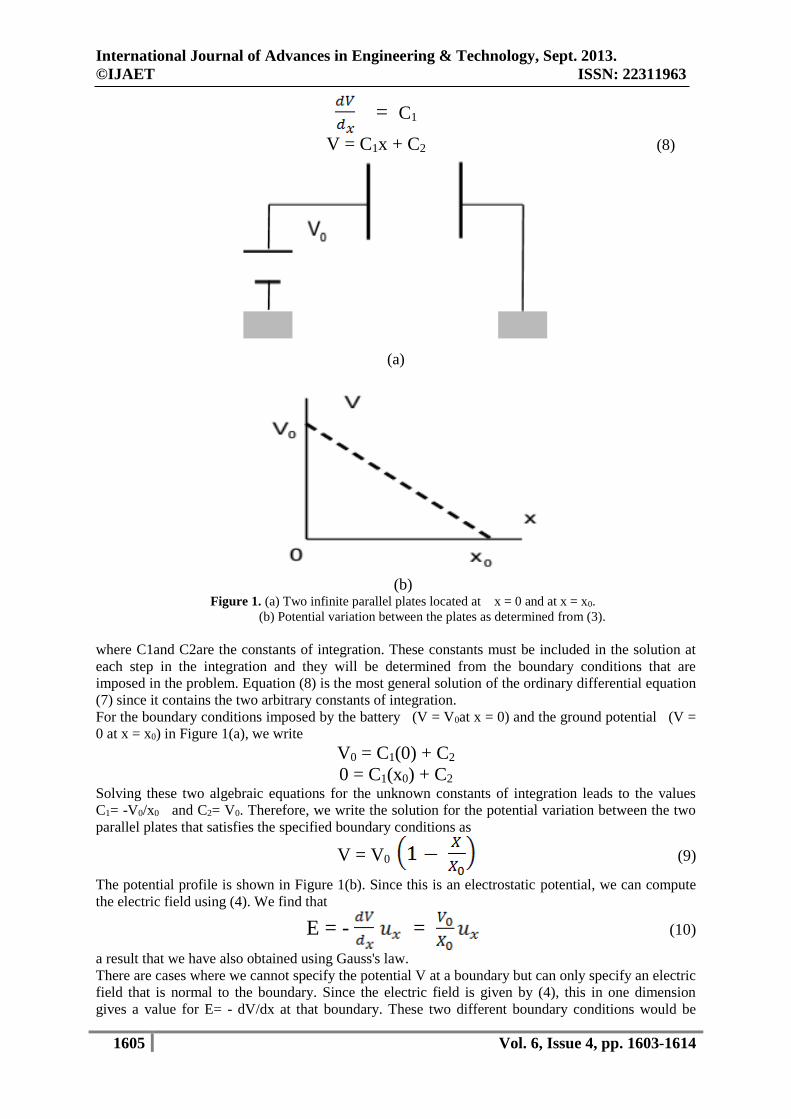
In order to conceptualize the method, we will calculate the potential variation between two infinite
parallel metal plates located in a vacuum as shown in Figure 1(a). This will require solving Laplace's
equation in one dimension and it will yield a result that approximates the potential distribution in a
parallel plate capacitor where the separation between the plates is much less than any transverse
dimension. Since the plates are assumed to be infinite and the conductivity of these metal plates is
very high, they can be assumed to be equipotential surfaces. We can think just that these metal plates
have zero resistance. Hence, in the y and the z coordinates, we can postulate with a high degree of
confidence that
Since there is no variation of the potential in two of the three independent variables, we can let the
remaining partial derivative that appears in Laplace's equation become an ordinary differential one.
Hence, the one-dimensional Laplace's equation is
(7)
Let us assume that the plate at x = 0 to be at a potential V = V0 and that the plate at x = x0 is
connected to ground and therefore has the potential V = 0. These are the boundary conditions for this
problem. The solution of (7) is found by integrating this equation twice
International Journal of Advances in Engineering & Technology, Sept. 2013.
©IJAET ISSN: 22311963
1605 Vol. 6, Issue 4, pp. 1603-1614
= C1
V = C1x + C2 (8)
(a)
(b)
Figure 1. (a) Two infinite parallel plates located at x = 0 and at x = x0. (b) Potential variation between the plates as determined from (3).
where C1and C2are the constants of integration. These constants must be included in the solution at
each step in the integration and they will be determined from the boundary conditions that are
imposed in the problem. Equation (8) is the most general solution of the ordinary differential equation
(7) since it contains the two arbitrary constants of integration.
For the boundary conditions imposed by the battery (V = V0at x = 0) and the ground potential (V =
0 at x = x0) in Figure 1(a), we write
V0 = C1(0) + C2
0 = C1(x0) + C2
Solving these two algebraic equations for the unknown constants of integration leads to the values
C1= -V0/x0 and C2= V0. Therefore, we write the solution for the potential variation between the two
parallel plates that satisfies the specified boundary conditions as
V = V0 (9)
The potential profile is shown in Figure 1(b). Since this is an electrostatic potential, we can compute
the electric field using (4). We find that
E = - = (10)
a result that we have also obtained using Gauss's law.
There are cases where we cannot specify the potential V at a boundary but can only specify an electric
field that is normal to the boundary. Since the electric field is given by (4), this in one dimension
gives a value for E= - dV/dx at that boundary. These two different boundary conditions would be
International Journal of Advances in Engineering & Technology, Sept. 2013.
©IJAET ISSN: 22311963
1606 Vol. 6, Issue 4, pp. 1603-1614
analogous to a metal plate being clamped atone edge or passing between two rollers that specify the
slope of the plate at that edge. The vertical height of the rollers could, however, be arbitrarily adjusted
in a rolling mill.
III. ANALYTICAL SOLUTION OF A TWO DIMENSIONAL
In this paper, we will introduce the methodical procedure to effect the solution of the type of problem
that is governed by Poisson's or Laplace's equation in higher dimensions. The technique that will be
employed to obtain this solution is the powerful "method of separation of variables." It is
pedagogically convenient to introduce the technique with an example and then carefully work through
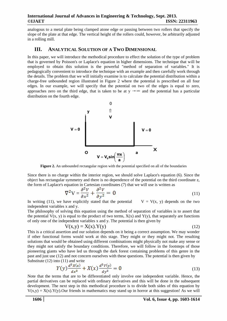
the details. The problem that we will initially examine is to calculate the potential distribution within a
charge-free unbounded region illustrated in Figure 2 where the potential is prescribed on all four
edges. In our example, we will specify that the potential on two of the edges is equal to zero,
approaches zero on the third edge, that is taken to be at y →∞ and the potential has a particular
distribution on the fourth edge.
Figure 2. An unbounded rectangular region with the potential specified on all of the boundaries
Since there is no charge within the interior region, we should solve Laplace's equation (6). Since the
object has rectangular symmetry and there is no dependence of the potential on the third coordinate z,
the form of Laplace's equation in Cartesian coordinates (7) that we will use is written as
V = (11)
In writing (11), we have explicitly stated that the potential V = V(x, y) depends on the two
independent variables x and y.
The philosophy of solving this equation using the method of separation of variables is to assert that
the potential V(x, y) is equal to the product of two terms, X(x) and Y(y), that separately are functions
of only one of the independent variables x and y. The potential is then given by
V(x,y) = X(x).Y(y) (12) This is a critical assertion and our solution depends on it being a correct assumption. We may wonder
if other functional forms would work at this stage. They might or they might not. The resulting
solutions that would be obtained using different combinations might physically not make any sense or
they might not satisfy the boundary conditions. Therefore, we will follow in the footsteps of those
pioneering giants who have led us through the dark forest containing problems of this genre in the
past and just use (12) and not concern ourselves with these questions. The potential is then given by
Substitute (12) into (11) and write
(13)
Note that the terms that are to be differentiated only involve one independent variable. Hence, the
partial derivatives can be replaced with ordinary derivatives and this will be done in the subsequent
development. The next step in this methodical procedure is to divide both sides of this equation by
V(x,y) = X(x).Y(y).Our friends in mathematics may stand up in horror at this suggestion! As we will
International Journal of Advances in Engineering & Technology, Sept. 2013.
©IJAET ISSN: 22311963
1607 Vol. 6, Issue 4, pp. 1603-1614
later see, one of these terms could be zero at one or more points in space. Recall what a calculator or
computer tells us when we do this "evil" deed of dividing by zero! With this warning in hand and with
a justified amount of trepidation, let us see what does result from this action. In our case, the end will
justify the means. We find that
(14)
The first term on the left side of (14) is independent of the variable y. As far as the variable y, it can
be considered to be a constant that we will take to be - . Using a similar argument, the second term
on the left side of (14) is independent of the variable x and it also can be replaced with another
constant that will be written as + . Therefore, (14) can be written as two ordinary differential
equations and one algebraic equation:
(15)
(16)
(17)
A pure mathematician would have just written these three equations down by inspection in order to
avoid any problems with dividing by zero that we have so cavalierly glossed over.
The two second-order ordinary differential equations can be easily solved. We write that
(18)
(19)
where we include the constants of integration, C1to C4. Let us now determine these constants of
integration from the boundary conditions imposed in Figure 2. From (12), we note that the potential
V(x, y) is determined by multiplying the solution X(x) with Y(y). Therefore, we can specify the
constants by examining each term separately. For any value of y at x = 0, the potential V(0, y) is equal
to zero. The only way that we can satisfy this requirement is to let the constant: C2= 0 since cos 0 = 1.
Nothing can be stated about the constant C1from this particular boundary condition since sin 0 = 0.
For any value of x and in the limit of y →∞, the potential V (x,y→∞). This specifies that the constant
C3= 0 since the term exp( kyy) →∞ as y→∞. The constant C4remains undetermined from the
application of this boundary condition. The potential on the third surface V(a, y) is also specified to be
zero at x = a from which we conclude that Kx = n π/a since sin nπ = 0 . From (17), we also write that
the constants Ky = Kx . With these values for the constants, our solution V(x,y) = X(x).Y(y) becomes
(20)
For this example, the integer n will take the value of n = 1 in order to fit the fourth boundary condition
at y = 0. Finally, the product of the two constants [C1C4] that is just another constant is set equal to
V0. The potential in this channel finally is given by
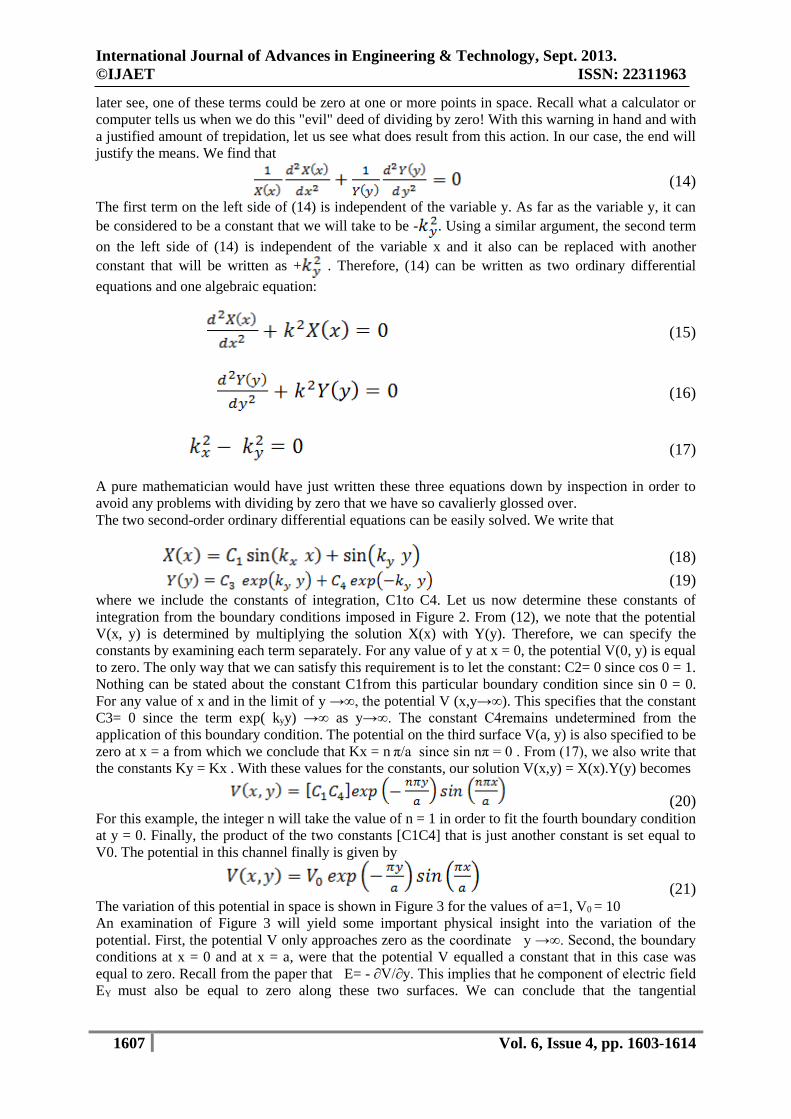
(21) The variation of this potential in space is shown in Figure 3 for the values of a=1, V0 = 10
An examination of Figure 3 will yield some important physical insight into the variation of the
potential. First, the potential V only approaches zero as the coordinate y →∞. Second, the boundary
conditions at x = 0 and at x = a, were that the potential V equalled a constant that in this case was
equal to zero. Recall from the paper that E= - ∂V/∂y. This implies that he component of electric field
EY must also be equal to zero along these two surfaces. We can conclude that the tangential
International Journal of Advances in Engineering & Technology, Sept. 2013.
©IJAET ISSN: 22311963
1608 Vol. 6, Issue 4, pp. 1603-1614
component of electric field adjacent to an equipotential surface will be equal to zero. This conclusion
will be of importance in several later calculations
Figure 3 Variation of the potential within the region for the prescribed boundary conditions depicted in Figure
The procedure that we have conducted is the determination of the solution of a partial differential
equation. Let us recapitulate the procedure before attacking a slightly more difficult problem.
(1) The proper form of the Laplacian operator ∇2V for the coordinate system of interest was chosen.
This choice was predicated on the symmetry and the boundary conditions of the problem.
(2) The potential V(x,y) that depended on two independent variables was separated into two
dependent variables that individually depended on only one of the independent variables. This
allowed us to write the partial differential equation as a set of ordinary differential equations and
an algebraic equation by assuming that the solution could be considered as a product of the
individual functions of the individual independent variables.
(3) Each of the ordinary differential equations was solved that led to several constants of integration.
The solution of each ordinary differential equation was multiplied together to obtain the general
solution of the partial differential equation.
(4) The arbitrary constants of integration that appeared when the ordinary differential equations were
solved were determined such that the boundary conditions would be satisfied. The solution for a
particular problem has now been obtained. Note that this step is similar to the methodical procedure
that we employed in the one dimensional case.
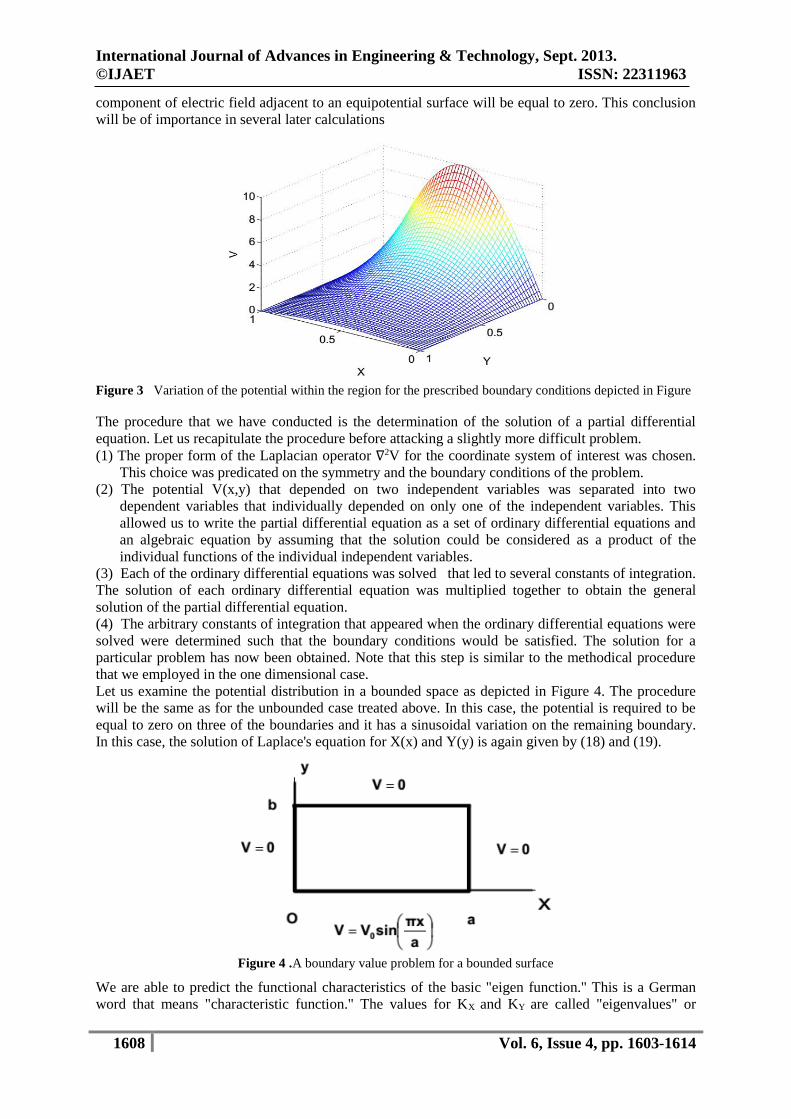
Let us examine the potential distribution in a bounded space as depicted in Figure 4. The procedure
will be the same as for the unbounded case treated above. In this case, the potential is required to be
equal to zero on three of the boundaries and it has a sinusoidal variation on the remaining boundary.
In this case, the solution of Laplace's equation for X(x) and Y(y) is again given by (18) and (19).
Figure 4 .A boundary value problem for a bounded surface
We are able to predict the functional characteristics of the basic "eigen function." This is a German
word that means "characteristic function." The values for KX and KY are called "eigenvalues" or
International Journal of Advances in Engineering & Technology, Sept. 2013.
©IJAET ISSN: 22311963
1609 Vol. 6, Issue 4, pp. 1603-1614
characteristic values. In this case again, the eigenvalue KX = KY as determined from (16). We may also
find this function referred to as a proper function.
The constants are again determined by the boundary conditions. From (17), the constant C2= 0 again
since the potential V = 0 at x = 0. The constant KX = nπ/a since the potential V = 0 at x = a – these
are the eigenvalues of the problem. From (18), we write
(22) since the potential V = 0 at y = b, which yields a relationship between C3and C4. Therefore, the
potential within the enclosed region specified in Figure 4 can be written as
(23) Or
(24)
The constants within the square brackets will be determined from the remaining boundary condition at
y = 0. The boundary condition at y = 0 states that V = V0 sin(πx/a) for 0 ≤x ≤a. Hence, the integer
n = 1 and
(25)
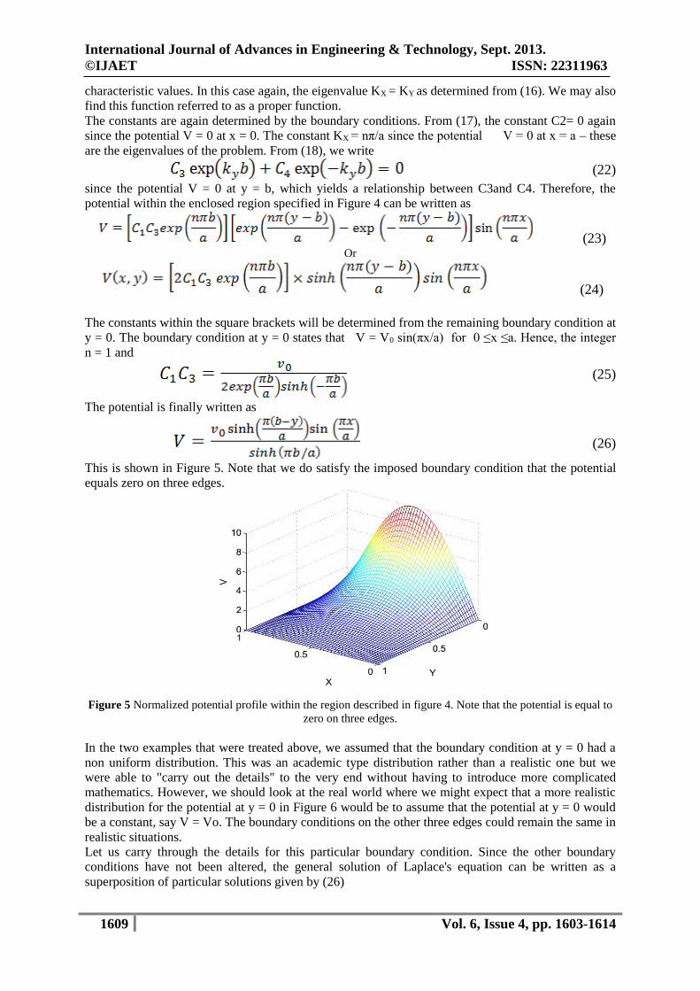
The potential is finally written as
(26)
This is shown in Figure 5. Note that we do satisfy the imposed boundary condition that the potential
equals zero on three edges.
Figure 5 Normalized potential profile within the region described in figure 4. Note that the potential is equal to
zero on three edges.
In the two examples that were treated above, we assumed that the boundary condition at y = 0 had a
non uniform distribution. This was an academic type distribution rather than a realistic one but we
were able to "carry out the details" to the very end without having to introduce more complicated
mathematics. However, we should look at the real world where we might expect that a more realistic
distribution for the potential at y = 0 in Figure 6 would be to assume that the potential at y = 0 would
be a constant, say V = Vo. The boundary conditions on the other three edges could remain the same in
realistic situations.
Let us carry through the details for this particular boundary condition. Since the other boundary
conditions have not been altered, the general solution of Laplace's equation can be written as a
superposition of particular solutions given by (26)
International Journal of Advances in Engineering & Technology, Sept. 2013.
©IJAET ISSN: 22311963
1610 Vol. 6, Issue 4, pp. 1603-1614
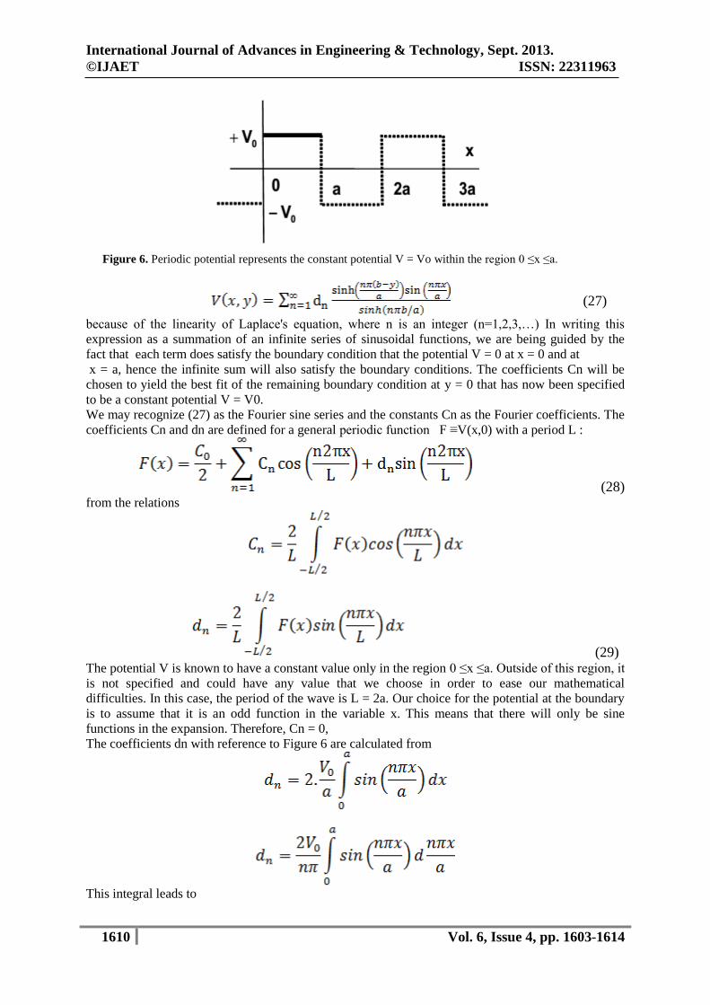
Figure 6. Periodic potential represents the constant potential V = Vo within the region 0 ≤x ≤a.
(27)
because of the linearity of Laplace's equation, where n is an integer (n=1,2,3,…) In writing this
expression as a summation of an infinite series of sinusoidal functions, we are being guided by the
fact that each term does satisfy the boundary condition that the potential V = 0 at x = 0 and at
x = a, hence the infinite sum will also satisfy the boundary conditions. The coefficients Cn will be
chosen to yield the best fit of the remaining boundary condition at y = 0 that has now been specified
to be a constant potential V = V0.
We may recognize (27) as the Fourier sine series and the constants Cn as the Fourier coefficients. The
coefficients Cn and dn are defined for a general periodic function F ≡V(x,0) with a period L :
(28) from the relations
(29) The potential V is known to have a constant value only in the region 0 ≤x ≤a. Outside of this region, it
is not specified and could have any value that we choose in order to ease our mathematical
difficulties. In this case, the period of the wave is L = 2a. Our choice for the potential at the boundary
is to assume that it is an odd function in the variable x. This means that there will only be sine
functions in the expansion. Therefore, Cn = 0,
The coefficients dn with reference to Figure 6 are calculated from
This integral leads to
International Journal of Advances in Engineering & Technology, Sept. 2013.
©IJAET ISSN: 22311963
1611 Vol. 6, Issue 4, pp. 1603-1614
(30) The potential is given by (28) with the coefficients defined in (30)
(31) This is called the analytical solution of two dimensional equation.
IV. FINITE ELEMENT METHOD USING MATLAB
There are different methods for the numerical solution of the two dimensional Laplace’s and
Poisson’s equation. Some of the techniques are based on a differential formulation that was
introduced earlier [2]. The Finite difference method is considered here and the Finite element method is
discussed in the next paper. Other techniques are based on the integral formulation of the boundary
value problems such as the Method of moments is described later. The boundary value problems
become more complicated in the presence of dielectric interfaces which are also considered in this
paper.
The finite difference method (FDM) considered here is an extension of the method already applied to
a one-dimensional problem. This method allows MATLAB to be more directly involved in the
solution of the boundary value problems. We will discuss this method here using a problem that is
similar to that presented in equation. We will describe the technique to obtain and to solve a suitable
set of coupled equations that can be interpreted as a matrix equation.
he algorithm that we use is based on the approximation for the second derivatives in Cartesian
coordinates. In this case, we assume a square grid with a step size h in both directions for a two-
dimensional calculation
2
2
1V(x, y) V x h, y V x h, y
h
V x, y h V x, y h 4V x, y
(32)
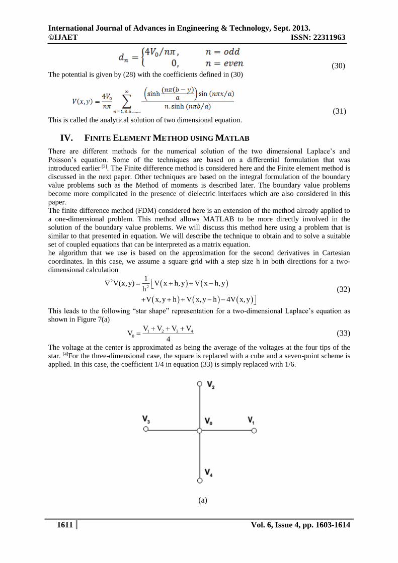
This leads to the following “star shape” representation for a two-dimensional Laplace’s equation as
shown in Figure 7(a)
1 2 3 40
V V V VV
4
(33)
The voltage at the center is approximated as being the average of the voltages at the four tips of the
star. [4]For the three-dimensional case, the square is replaced with a cube and a seven-point scheme is
applied. In this case, the coefficient 1/4 in equation (33) is simply replaced with 1/6.
(a)
International Journal of Advances in Engineering & Technology, Sept. 2013.
©IJAET ISSN: 22311963
1612 Vol. 6, Issue 4, pp. 1603-1614
(b)
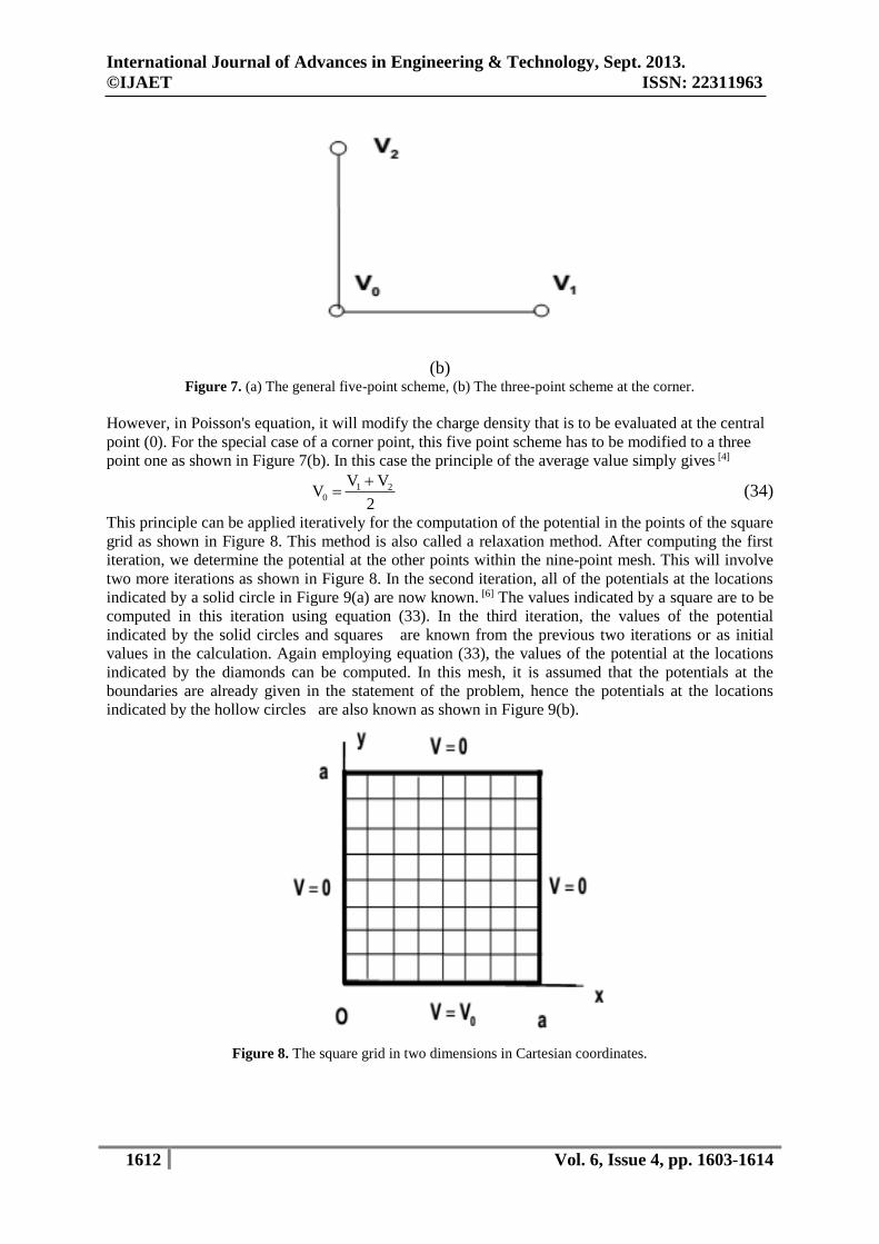
Figure 7. (a) The general five-point scheme, (b) The three-point scheme at the corner.
However, in Poisson's equation, it will modify the charge density that is to be evaluated at the central
point (0). For the special case of a corner point, this five point scheme has to be modified to a three
point one as shown in Figure 7(b). In this case the principle of the average value simply gives [4]
1 20
V VV
2
(34)
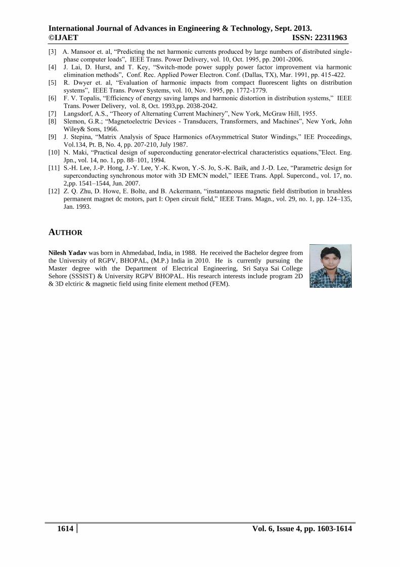
This principle can be applied iteratively for the computation of the potential in the points of the square
grid as shown in Figure 8. This method is also called a relaxation method. After computing the first
iteration, we determine the potential at the other points within the nine-point mesh. This will involve
two more iterations as shown in Figure 8. In the second iteration, all of the potentials at the locations
indicated by a solid circle in Figure 9(a) are now known. [6] The values indicated by a square are to be
computed in this iteration using equation (33). In the third iteration, the values of the potential
indicated by the solid circles and squares are known from the previous two iterations or as initial
values in the calculation. Again employing equation (33), the values of the potential at the locations
indicated by the diamonds can be computed. In this mesh, it is assumed that the potentials at the
boundaries are already given in the statement of the problem, hence the potentials at the locations
indicated by the hollow circles are also known as shown in Figure 9(b).
Figure 8. The square grid in two dimensions in Cartesian coordinates.
International Journal of Advances in Engineering & Technology, Sept. 2013.
©IJAET ISSN: 22311963
1613 Vol. 6, Issue 4, pp. 1603-1614
(a)
Figure 9. The second and third iterations. (a) The values of the potential indicated by the solid circles are
known. The values at the locations of the solid squares are computed in the second iteration. (b) The potentials
at the boundaries indicated by the hollow circles are assumed to be known. The potentials at the locations
indicated by the diamonds are computed in the third iteration.
This iterative procedure can continue until the computed values at all of the points in the decreasing
meshes become closer to each other. The accuracy of the calculation can be insured by repeating the
calculation with a different initial mesh size. A mesh with a shape and orientation that is different than
the one used here could also be employed in a numerical calculation.[8] This is particularly useful in
calculations involving unusual shapes. It is also possible to scale the various dimensions in order to
use this particular mesh. A critical restriction is also found on the square mesh size in that the first
point must be in the center of the square. This point will be evaluated from the four boundaries of the
square. This will restrict the number of internal points N of the square to contain the following
number of points
12; 32; 72, 152; 312’ 632;… [2N-1]2 (35)
This is called the array.
V. CONCLUSION
The numerical techniques that were introduced here are also applicable to three-dimensional problems
that may be later encountered. As presented in this paper, all of the methods assume linearity which
leads to linear superposition principles. However, you will frequently encounter nonlinearity in nature
which will lead to significant alterations in your method of obtaining a solution. Numerical questions
concerning other specific programming solving boundary value problems for potentials has led us to
certain general conclusions concerning the methodical procedure. First, nature has given us certain
physical phenomena that can be described by partial or ordinary differential equations. In many cases,
these equations can be solved analytically. Other cases may require numerical solutions. The
analytical solutions contain constants of integration. Nature also provides us with enough information
that will allow us to evaluate these constants and thus obtain the solution for the problem. Assuming
that neither mathematical nor numerical mistakes have been made, we can rest assured that this is the
solution.
REFERENCES
[1] IEEE Task Force, “Effects of harmonics on equipment”, IEEE Trans. Power Delivery, vol. 8, Apr. 1993,
pp. 672-680.
[2] IEEE Task Force, “The effects of power system harmonics n power system equipment and loads”, IEEE
Trans. Power Apparatus and Systems, vol. PAS-104, Sept. 1985, pp. 2555-2563.
International Journal of Advances in Engineering & Technology, Sept. 2013.
©IJAET ISSN: 22311963
1614 Vol. 6, Issue 4, pp. 1603-1614
[3] A. Mansoor et. al, “Predicting the net harmonic currents produced by large numbers of distributed single-
phase computer loads”, IEEE Trans. Power Delivery, vol. 10, Oct. 1995, pp. 2001-2006.
[4] J. Lai, D. Hurst, and T. Key, “Switch-mode power supply power factor improvement via harmonic
elimination methods”, Conf. Rec. Applied Power Electron. Conf. (Dallas, TX), Mar. 1991, pp. 415-422.
[5] R. Dwyer et. al, “Evaluation of harmonic impacts from compact fluorescent lights on distribution
systems”, IEEE Trans. Power Systems, vol. 10, Nov. 1995, pp. 1772-1779.
[6] F. V. Topalis, “Efficiency of energy saving lamps and harmonic distortion in distribution systems,” IEEE
Trans. Power Delivery, vol. 8, Oct. 1993,pp. 2038-2042.
[7] Langsdorf, A.S., “Theory of Alternating Current Machinery”, New York, McGraw Hill, 1955.
[8] Slemon, G.R.; “Magnetoelectric Devices - Transducers, Transformers, and Machines”, New York, John
Wiley& Sons, 1966.
[9] J. Stepina, “Matrix Analysis of Space Harmonics ofAsymmetrical Stator Windings,” IEE Proceedings,
Vol.134, Pt. B, No. 4, pp. 207-210, July 1987.
[10] N. Maki, “Practical design of superconducting generator-electrical characteristics equations,”Elect. Eng.
Jpn., vol. 14, no. 1, pp. 88–101, 1994.
[11] S.-H. Lee, J.-P. Hong, J.-Y. Lee, Y.-K. Kwon, Y.-S. Jo, S.-K. Baik, and J.-D. Lee, “Parametric design for
superconducting synchronous motor with 3D EMCN model,” IEEE Trans. Appl. Supercond., vol. 17, no.
2,pp. 1541–1544, Jun. 2007.
[12] Z. Q. Zhu, D. Howe, E. Bolte, and B. Ackermann, “instantaneous magnetic field distribution in brushless
permanent magnet dc motors, part I: Open circuit field,” IEEE Trans. Magn., vol. 29, no. 1, pp. 124–135,
Jan. 1993.
AUTHOR
Nilesh Yadav was born in Ahmedabad, India, in 1988. He received the Bachelor degree from
the University of RGPV, BHOPAL, (M.P.) India in 2010. He is currently pursuing the
Master degree with the Department of Electrical Engineering, Sri Satya Sai College
Sehore (SSSIST) & University RGPV BHOPAL. His research interests include program 2D
& 3D elctiric & magnetic field using finite element method (FEM).