Analysis of radiation modeling for turbulentcombustion : development of a methodology tocouple turbulent combustion and radiative heat

transfer in LES

POITOU DamienCERFACS

42, Avenue Gaspard Coriolis31057 Toulouse Cedex 01

France.Email : poitou@cerfacs.fr

EL HAFI MounaCentre RAPSODEE

Ecole des Mines d’AlbiCampus Jarlard

81013 ALBIFrance

CUENOT BenedicteCERFACS

42, Avenue Gaspard Coriolis31057 Toulouse Cedex 01

France.

ABSTRACT

Radiation exchanges must be taken into account to improve Large Eddy Simulation (LES) prediction of turbu-lent combustion, in particular for wall heat fluxes. Because of its interaction with turbulence and its impact onthe formation of polluting species, unsteady coupled calculations are required. This work constitutes a first steptowards coupled LES-radiation simulations, selecting the optimal methodology based on systematic comparisonsof accuracy and CPU cost. Radiation is solved with the Discrete Ordinate Method (DOM) and different spec-tral models. To reach the best compromise between accuracy and CPU time, the performance of various spectralmodels and discretizations (angular, temporal and spatial) is studied. It is shown that the use of a global spectralmodel combined with a mesh coarsening (compared to the LES mesh) and a minimal coupling frequency Nit allowsto compute one radiative solution faster than Nit LES iterations, while keeping a good accuracy. It also appearsthan the impact on accuracy of the angular discretization in the DOM is very small compared to the impact of thespectral model. The determined optimal methodology may be used to perform unsteady coupled calculations ofturbulent combustion with radiation.

IntroductionRadiation is one important heat transfer phenomenon in combustion devices. Previous studies have shown that is is

necessary to solve radiative heat transfer to improve combustion simulation results [1, 2, 3]. Heat losses may change thetemperature of the flame by more than 100 K which can significantly modify the chemical kinetics, cf. polluting species likeNOx, CO, or soot particles in luminous flames. Moreover, the radiative heat flux must be determined to evaluate correctlythe thermal exchanges with walls. Due to the complexity of radiation and the nonlinear interactions between reacting flows,heat transfer and turbulence perform coupled simulations in practical situations is a challenge.

While Reynolds Average Navier-Stokes (RANS) provide only averaged results, Large Eddy Simulation (LES) [4, 5] isable to predict instantaneous flow characteristics. Also, LES is in principle more accurate as the large flow scales are resolvedexplicitly while only the small scales are modeled. Many authors demonstrated the advantages of LES in application to gasturbine engines [6], laboratory flames [7] or in other combustion systems [8, 9].

Radiation may be calculated from a steady flame solution to study wall heat fluxes for example. However the interactionwith the turbulence may have a strong impact on radiation : this is referred as the Turbulence-Radiation Interaction (TRI)

problem which has been studied by many authors (see [10] for a review on this topic). To take into account the interactionwith turbulence and chemistry coupled calculations are required.

Literature about radiation in LES is limited. Only few papers present detailed radiation calculations in configurationsinvolving a high number of mesh cells (more than a million). Desjardin et al. [11] have coupled combustion and radiationin a bi-dimensional configuration of a non-premixed acetylene/air planar jet flame with 16 000 cells. The gas is transparentand only the absorption of soot is considered. The radiative transfer is solved in a finite volume approach using the DiscreteOrdinate Method (DOM). Jones et al. [12] have also used DOM with Sn quadratures in a LES of a gas turbine combustorusing a 16 000 cells mesh and a gray gas spectral model. Joseph et al. [13] developed a DOM solver for unstructuredmeshes to compute radiation in the PRECCINSTA burner [14] where the swirled flames is typical of turbo-engines. Themesh contained 138 000 cells and a narrow band model (SNBcK) was used. However the radiation and LES calculationwere not coupled. More recently Dos Santos et al. [3, 15] worked on the feasibility of the coupling between turbulentcombustion and detailed radiation in practical systems. First a 2D situation has been studied in [15] using a raytracingmethod. Then a 3D premixed propane/air flame stabilized behind a triangular flame holder [16, 17] was calculated withcoupled DOM-LES approaches [3]. Preliminary results demonstrated the feasibility of the coupling and showed first trendsof the impact of radiation on flame dynamics. Due to the very high computing cost of both LES and radiation simulations,further investigation is needed to optimize the choice of the models and their coupling to provide a good compromise betweenCPU time and accuracy.

The main objective of this work is to propose an efficient and accurate radiation solver adapted to LES. This meansin particular that the ratio between CPU time of DOM and LES must be close to 1. This will be achieved by an optimalchoice of models and parameters, such as the radiative properties model, the subcycling frequency, the mesh resolution, thedistribution over parallel processors or the number of directions to discretize the solid angle in DOM.

In the following, section one describes the test configuration which is the same as in [3, 15]. Then, the LES calculationof this configuration is briefly presented. In the second section, the numerical method and radiation models are detailed.The approach to couple combustion with radiation is presented in the third section where a subcycling scheme is defined. Insection four, the influence of the physical and numerical parameters of the radiation model is studied and analyzed to deter-mine the best compromise between calculation time and accuracy. In particular the influence of the angular discretizationand of the spectral model are discussed. In section five the effect of the mesh resolution on radiation results is investigatedwhereas in section six the influence of the wall reflection is addressed. Finally the impact of all parameters on the radiativetime calculation with the associated level of accuracy is summarized and compared to the combustion calculation time.

1 The test configuration1.1 Geometry

The test configuration was initially set up and studied experimentally by Knikker et al. [16, 17, 7] and is represented inFig. 1.

Fig. 1. Test configuration [16].

A premixed propane/air flow is injected into a rectangular combustor. The dimensions of the combustion chamber in

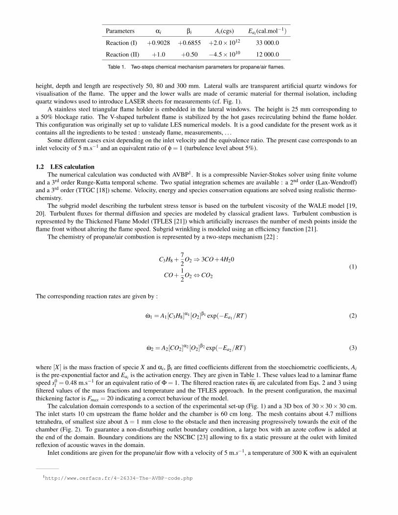
Parameters αi βi Ai(cgs) Eai (cal.mol−1)

Reaction (I) +0.9028 +0.6855 +2.0×1012 33 000.0

Reaction (II) +1.0 +0.50 −4.5×1010 12 000.0

Table 1. Two-steps chemical mechanism parameters for propane/air flames.

height, depth and length are respectively 50, 80 and 300 mm. Lateral walls are transparent artificial quartz windows forvisualisation of the flame. The upper and the lower walls are made of ceramic material for thermal isolation, includingquartz windows used to introduce LASER sheets for measurements (cf. Fig. 1).

A stainless steel triangular flame holder is embedded in the lateral windows. The height is 25 mm corresponding toa 50% blockage ratio. The V-shaped turbulent flame is stabilized by the hot gases recirculating behind the flame holder.This configuration was originally set up to validate LES numerical models. It is a good candidate for the present work as itcontains all the ingredients to be tested : unsteady flame, measurements, . . .

Some different cases exist depending on the inlet velocity and the equivalence ratio. The present case corresponds to aninlet velocity of 5 m.s−1 and an equivalent ratio of φ = 1 (turbulence level about 5%).

1.2 LES calculationThe numerical calculation was conducted with AVBP1. It is a compressible Navier-Stokes solver using finite volume

and a 3rd order Runge-Kutta temporal scheme. Two spatial integration schemes are available : a 2nd order (Lax-Wendroff)and a 3rd order (TTGC [18]) scheme. Velocity, energy and species conservation equations are solved using realistic thermo-chemistry.

The subgrid model describing the turbulent stress tensor is based on the turbulent viscosity of the WALE model [19,20]. Turbulent fluxes for thermal diffusion and species are modeled by classical gradient laws. Turbulent combustion isrepresented by the Thickened Flame Model (TFLES [21]) which artificially increases the number of mesh points inside theflame front without altering the flame speed. Subgrid wrinkling is modeled using an efficiency function [21].

The chemistry of propane/air combustion is represented by a two-steps mechanism [22] :

C3H8 +72

O2⇒ 3CO+4H20

CO+12

O2⇔CO2

(1)

The corresponding reaction rates are given by :

ω1 = A1[C3H8]α1 [O2]β1 exp(−Ea1/RT ) (2)

ω2 = A2[CO2]α2 [O2]β2 exp(−Ea2/RT ) (3)

where [X ] is the mass fraction of specie X and αi, βi are fitted coefficients different from the stoechiometric coefficients, Aiis the pre-exponential factor and Eai is the activation energy. They are given in Table 1. These values lead to a laminar flamespeed s0

l = 0.48 m.s−1 for an equivalent ratio of Φ = 1. The filtered reaction rates ωi are calculated from Eqs. 2 and 3 usingfiltered values of the mass fractions and temperature and the TFLES approach. In the present configuration, the maximalthickening factor is Fmax = 20 indicating a correct behaviour of the model.

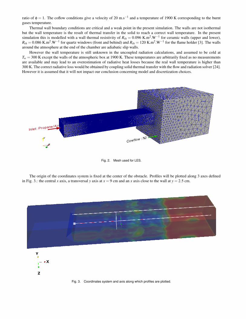
The calculation domain corresponds to a section of the experimental set-up (Fig. 1) and a 3D box of 30×30×30 cm.The inlet starts 10 cm upstream the flame holder and the chamber is 60 cm long. The mesh contains about 4.7 millionstetrahedra, of smallest size about ∆ = 1 mm close to the obstacle and then increasing progressively towards the exit of thechamber (Fig. 2). To guarantee a non-disturbing outlet boundary condition, a large box with an azote coflow is added atthe end of the domain. Boundary conditions are the NSCBC [23] allowing to fix a static pressure at the oulet with limitedreflexion of acoustic waves in the domain.

Inlet conditions are given for the propane/air flow with a velocity of 5 m.s−1, a temperature of 300 K with an equivalent

1http://www.cerfacs.fr/4-26334-The-AVBP-code.php

ratio of φ = 1. The coflow conditions give a velocity of 20 m.s−1 and a temperature of 1900 K corresponding to the burntgases temperature.

Thermal wall boundary conditions are critical and a weak point in the present simulation. The walls are not isothermalbut the wall temperature is the result of thermal transfer in the solid to reach a correct wall temperature. In the presentsimulation this is modelled with a wall thermal resistivity of Rth = 0.096 K.m2.W−1 for ceramic walls (upper and lower),Rth = 0.086 K.m2.W−1 for quartz windows (front and behind) and Rth = 120 K.m2.W−1 for the flame holder [3]. The wallsaround the atmosphere at the end of the chamber are adiabatic slip walls.

However the wall temperature is still unknown in the uncoupled radiation calculations, and assumed to be cold atTw = 300 K except the walls of the atmospheric box at 1900 K. These temperatures are arbitrarily fixed as no measurementsare available and may lead to an overestimation of radiative heat losses because the real wall temperature is higher than300 K. The correct radiative loss would be obtained by coupling solid thermal transfer with the flow and radiation solver [24].However it is assumed that it will not impact our conclusion concerning model and discretization choices.

Fig. 2. Mesh used for LES.

The origin of the coordinates system is fixed at the center of the obstacle. Profiles will be plotted along 3 axes definedin Fig. 3.: the central x axis, a transversal y axis at x = 9 cm and an x axis close to the wall at y = 2.5 cm.

Fig. 3. Coordinates system and axis along which profiles are plotted.

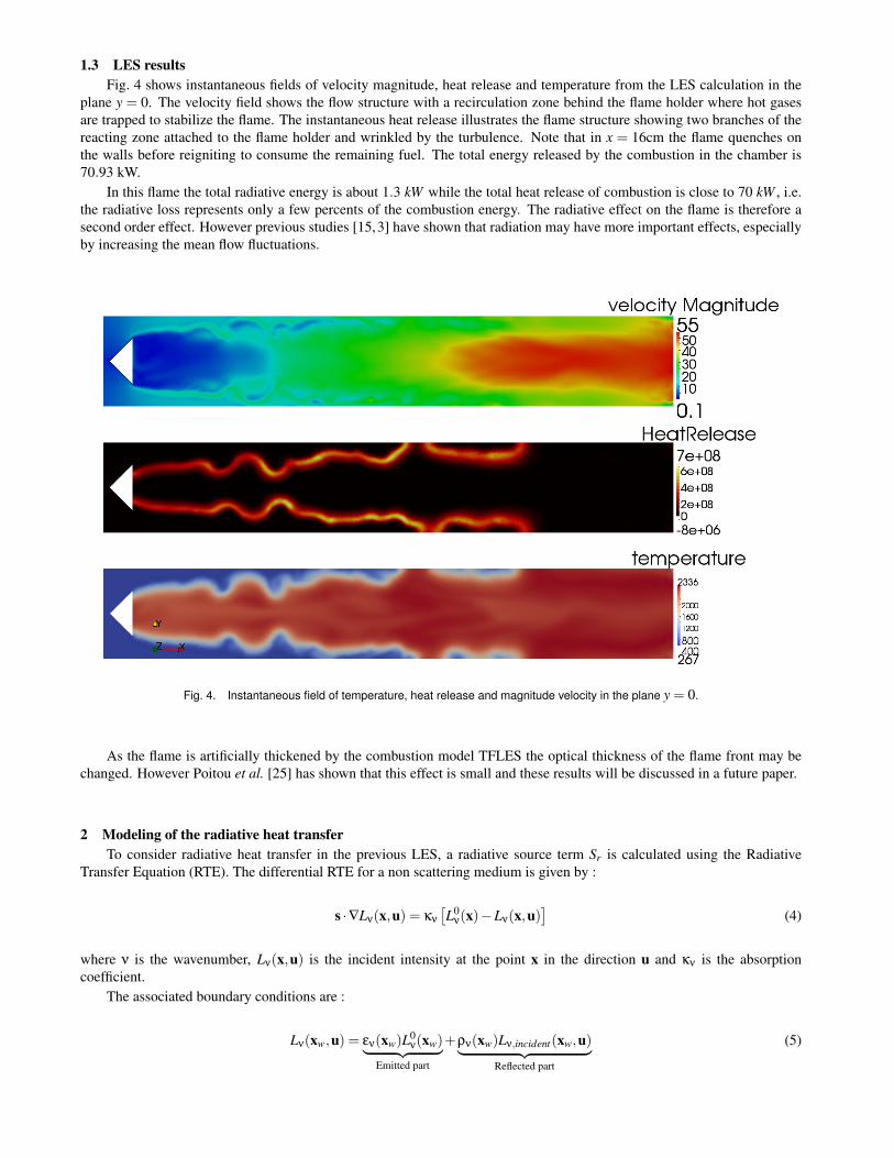
1.3 LES resultsFig. 4 shows instantaneous fields of velocity magnitude, heat release and temperature from the LES calculation in the

plane y = 0. The velocity field shows the flow structure with a recirculation zone behind the flame holder where hot gasesare trapped to stabilize the flame. The instantaneous heat release illustrates the flame structure showing two branches of thereacting zone attached to the flame holder and wrinkled by the turbulence. Note that in x = 16cm the flame quenches onthe walls before reigniting to consume the remaining fuel. The total energy released by the combustion in the chamber is70.93 kW.

In this flame the total radiative energy is about 1.3 kW while the total heat release of combustion is close to 70 kW , i.e.the radiative loss represents only a few percents of the combustion energy. The radiative effect on the flame is therefore asecond order effect. However previous studies [15,3] have shown that radiation may have more important effects, especiallyby increasing the mean flow fluctuations.

Fig. 4. Instantaneous field of temperature, heat release and magnitude velocity in the plane y = 0.

As the flame is artificially thickened by the combustion model TFLES the optical thickness of the flame front may bechanged. However Poitou et al. [25] has shown that this effect is small and these results will be discussed in a future paper.

2 Modeling of the radiative heat transferTo consider radiative heat transfer in the previous LES, a radiative source term Sr is calculated using the Radiative

Transfer Equation (RTE). The differential RTE for a non scattering medium is given by :

s ·∇Lν(x,u) = κν

[L0

ν(x)−Lν(x,u)]

(4)

where ν is the wavenumber, Lν(x,u) is the incident intensity at the point x in the direction u and κν is the absorptioncoefficient.

The associated boundary conditions are :

Lν(xw,u) = εν(xw)L0ν(xw)︸ ︷︷ ︸

Emitted part

+ρν(xw)Lν,incident(xw,u)︸ ︷︷ ︸Reflected part

(5)

where εν(xw) is the wall emissivity andρν(xw) the wall reflectivity (ρν(xw) = 1− εν(xw)).The source term Sr results from a double integration of the RTE in the physical and spectral spaces, leading to a

macroscopic source term which depends only on the position x :

Sr(x) =Z

∞

0κν

[4πL0

ν(x)−Z

4π

Lν(x,u)dΩ

]dν (6)

2.1 Angular discretizationVarious methods exist to perfom the angular integration over the discretized directions ui : Ray tracing methods follow-

ing optical paths, P1 methods uses spherical harmonics, Monte-Carlo methods calculate photon statistics with a high numberof absorption/diffusion events, . . . Here the Discrete Ordinate Method (DOM) is used which is a finite volume formulationof the RTE and offers a good compromise between accuracy and CPU time [26, 27, 14].

The radiative solver used in this work is PRISSMA2 [26, 2, 13, 27, 25]. The RTE is solved for a set of Ndir directions(ordinates), computing the integral over each ordinate by a numerical quadrature :

Z4π

f (u)dΩ'Ndir

∑i=1

wai f (ui) (7)

where ui are the discrete directions and ωai the associated weights of Sn quadratures determined from Truelove [28].

2.2 Spectral modelThe spectral dependency of the radiation is known for absorbing gases such as CO, CO2 and H2O and is very complex.

Line-by-line model gives the absorption for each frequency which implies rhe resolution of the RTE for at least one millionfrequencies in each direction. Narrow-band models such as SNBcK [29] offer a good accuracy with less calculations.Goutiere et al. have shown that the SNBcK model is very precise in combustion applications [29,30]. Finally global modelsallow to reduce the calculation to 3 to 15 spectral integrations in each direction.

In PRISSMA a series of spectral models are available. The SNBcK model is implemented with 371 narrow bands ofwidth ∆νi over the IR spectrum (wavelength in the range λ = [0.5;68 µm]): 367 bands from the SNB database from [31]more 4 bands in the visible for the radiation of soot. In each narrow band the Planck function is assumed to be constant.A re-arrangement called k-distribution allows to calculate the absorption coefficient in each band (i) with a Gauss-Legendrequadrature (over Nq points) of the cumulative function of the possible values of absorption. The final expression of theradiative source term is then :

Sr(x)'Nband

∑i=1

∆νi

[Nquad

∑j=1

ω jκi j

(4πL0

∆νi(x)−

Ndir

∑k=1

ωakLi j(x,uk)

)](8)

where ω j are the weights of the Gauss-Legendre quadrature, L0∆νi

(x) is the mean value of the Planck function on the ith

narrow band, κi j and Li j are respectively the absorption coefficient and the incident intensity for the quadrature point j in theith band.

Typically 5 quadrature point are used, corresponding to 371×5 = 1 800 integrations for each direction. The associatedcalculation time is still high and the SNBcK model is used here as a reference solution.

Two global models are also implemented in PRISSMA : the Weighted Sum of Gray Gases (WSGG) model [32] and theFull Spectrum SNBcK (FS-SNBcK) model [33, 34]. Such models are fast but their accuracy must be carefully checked.

A previous study has shown the validity limits for the global model FS-SNBcK [34] for combustion applications. Forthis model the macroscopic source term Sr is given by :

Sr(x)'Nq

∑j=1

ω jκ j

(4σT 4(x)−

Ndir

∑k=1

ωakL j(x,uk)

)(9)

where ω j are the weights of the Gauss-Legendre quadrature over the full spectrum.

2PRISSMA: Parallel RadIation Solver with Spectral integration on Multicomponent mediA, http://www.cerfacs.fr/prissma

This model is equivalent to the WSGG approach, using a partial intensity L j with the absorption coefficient κ j for eachquadrature point j. With the FS-SNBcK model the gray gas j is reconstructed from the narrow band properties [34]. TheWSGG model suffers from an important lack of accuracy, near high gradients of temperature. Moreover it uses assumptionssuch as constant ratio for CO2/H2O, no absorption of CO, . . . which may be not correct. However it represents a reference asthe shortest calculation time model.

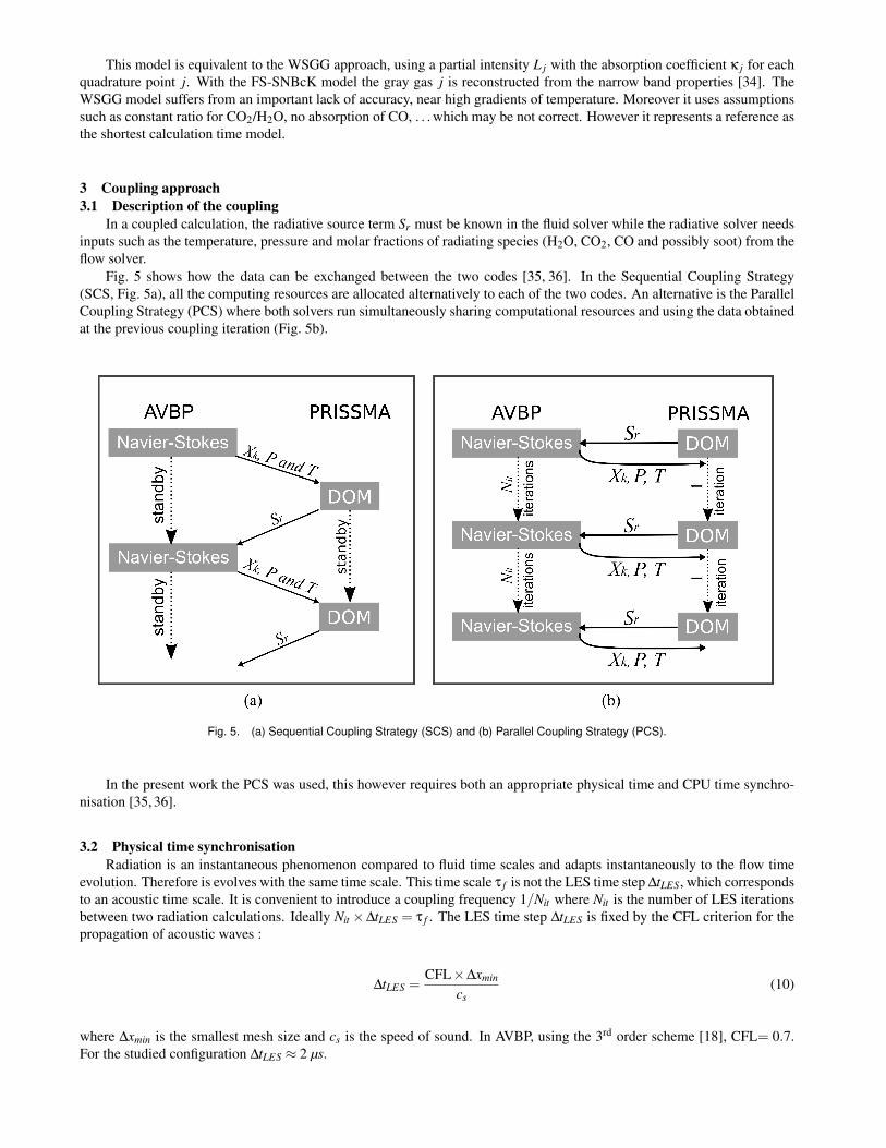
3 Coupling approach3.1 Description of the coupling

In a coupled calculation, the radiative source term Sr must be known in the fluid solver while the radiative solver needsinputs such as the temperature, pressure and molar fractions of radiating species (H2O, CO2, CO and possibly soot) from theflow solver.

Fig. 5 shows how the data can be exchanged between the two codes [35, 36]. In the Sequential Coupling Strategy(SCS, Fig. 5a), all the computing resources are allocated alternatively to each of the two codes. An alternative is the ParallelCoupling Strategy (PCS) where both solvers run simultaneously sharing computational resources and using the data obtainedat the previous coupling iteration (Fig. 5b).

Fig. 5. (a) Sequential Coupling Strategy (SCS) and (b) Parallel Coupling Strategy (PCS).

In the present work the PCS was used, this however requires both an appropriate physical time and CPU time synchro-nisation [35, 36].

3.2 Physical time synchronisationRadiation is an instantaneous phenomenon compared to fluid time scales and adapts instantaneously to the flow time

evolution. Therefore is evolves with the same time scale. This time scale τ f is not the LES time step ∆tLES, which correspondsto an acoustic time scale. It is convenient to introduce a coupling frequency 1/Nit where Nit is the number of LES iterationsbetween two radiation calculations. Ideally Nit ×∆tLES = τ f . The LES time step ∆tLES is fixed by the CFL criterion for thepropagation of acoustic waves :

∆tLES =CFL×∆xmin

cs(10)

where ∆xmin is the smallest mesh size and cs is the speed of sound. In AVBP, using the 3rd order scheme [18], CFL= 0.7.For the studied configuration ∆tLES ≈ 2 µs.

The radiative source term changes with the convection of hot gas [37] and Wang [38]. The flow time scale is evaluatedas:

τ f =∆xmin

u(11)

where u is the bulk flow velocity.Thus the radiative source term must be updated after Nit LES iterations such as :

Nit =τ f

∆tLES=

cs

0.7×u=

10.7M

(12)

For the low-Mach flows considered here Nit ∼ 100. The coupling frequency has also been studied on the same configurationby Dos Santos et al. [15, 3] who tested different values from 20 to 500. They also found Nit = 100 is the best compromisebetween accuracy and computing time. It is therefore retained for the following study.

3.3 CPU time synchronisationKnowing the coupling frequency, the minimal CPU time is obtained if :

Nit × tCPULES = tCPU

Rad (13)

where tCPULES et tCPU

Rad are respectively the CPU time required for one fluid iteration and one radiative calculation. As bothsolvers are parallel, the restitution time for each code depends on the allocated number of processors :

tCPULES = α(PLES)× tCPU,1

LES /PLES

tCPURad = α(PRad)× tCPU,1

Rad /PRad(14)

where tCPU,1∗ is the CPU time for on 1 processor, P∗ the number of allocated processors and α∗(P∗) the speed-up factor. For

a code with a perfect speed-up this factor is equal to 1.Combining Eqs. 13 and 14 and for a total number of processors P = PLES +PRad , the final processor distribution is :

PLES =P

(tCPU,1Rad /tCPU,1

LES )/Nit +1

Prad = P−PLES

(15)

AVBP is parallelized with a domain decomposition which is very efficient on massively parallel architectures with aperfect speed-up factor up to 4 078 processors on IBM BlueGene/L [39]. PRISSMA uses two levels of parallelization. Thecalculation of the absorption coefficients is parallelized with a domain decomposition as it depends on local flow quantitiesonly. The integration of the incident intensity is also parallelized on the bands (for SNBcK model) and on the incidentdirections. As the integration of the incident intensity involves the whole domain the use of domain decomposition is notstraightforward for radiation. By now the good scalability of PRISSMA is limited to the number of processor equal to thenumber of directions used for the DOM (i.e. the speed up factor is equal to 1 until 24 processors for an S4 quadrature).This is a important limitation for coupled simulations on industrial configurations and the use of domain decomposition forradiation is currently investigated.

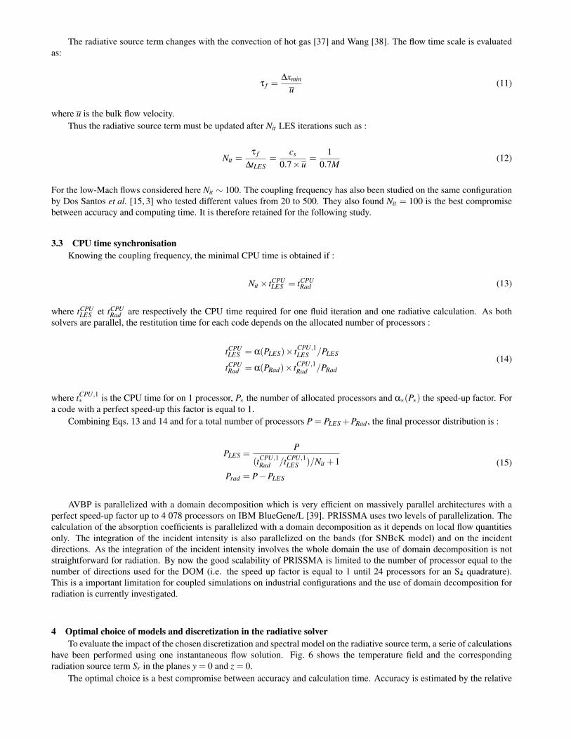
4 Optimal choice of models and discretization in the radiative solverTo evaluate the impact of the chosen discretization and spectral model on the radiative source term, a serie of calculations

have been performed using one instantaneous flow solution. Fig. 6 shows the temperature field and the correspondingradiation source term Sr in the planes y = 0 and z = 0.

The optimal choice is a best compromise between accuracy and calculation time. Accuracy is estimated by the relative

Fig. 6. Instantaneous fields of temperature and radiative source term Sr (W/m3) in the y = 0 et z = 0 planes.

error compared to a reference solution for the total radiative energy:

εtot =|〈ψ〉−

⟨ψre f

⟩|⟨

ψre f⟩ (16)

where 〈Ψ〉 is the total radiated energy.The mean relative error and its variance are also estimated along the central axis as:

ε =|Sr−Sr,re f |

Sr,re f

σ =√

ε2− ε2

(17)

where the overline denotes the average along the central axis.The calculation of radiation depends on the number of integration of the RTE integrations and the number of discretiza-

tion points, It can be written as :

tCPURad ∝ Ndir︸︷︷︸

Angular discretisation

×NBands×Nq︸ ︷︷ ︸Spectral model

×NPoints︸ ︷︷ ︸Mesh

(18)

In the next sections, the impact on the CPU time of each contributor (number of directions, spectral bands and meshpoints) is discussed.

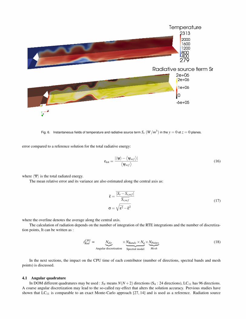
4.1 Angular quadratureIn DOM different quadratures may be used : SN means N(N +2) directions (S4 : 24 directions), LC11 has 96 directions.

A coarse angular discretization may lead to the so-called ray-effect that alters the solution accuracy. Previous studies haveshown that LC11 is comparable to an exact Monte-Carlo approach [27, 14] and is used as a reference. Radiation source

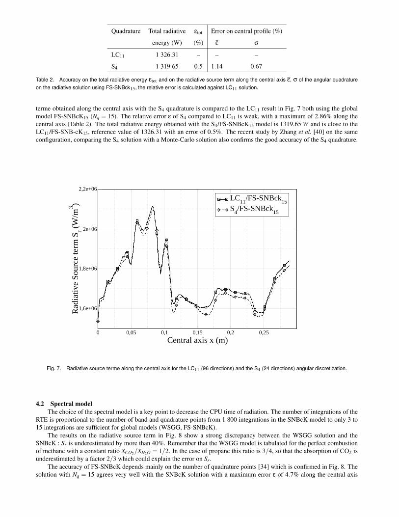
Quadrature Total radiative εtot Error on central profile (%)

energy (W) (%) ε σ

LC11 1 326.31 – – –

S4 1 319.65 0.5 1.14 0.67

Table 2. Accuracy on the total radiative energy εtot and on the radiative source term along the central axis ε, σ of the angular quadratureon the radiative solution using FS-SNBck15, the relative error is calculated against LC11 solution.

terme obtained along the central axis with the S4 quadrature is compared to the LC11 result in Fig. 7 both using the globalmodel FS-SNBcK15 (Nq = 15). The relative error ε of S4 compared to LC11 is weak, with a maximum of 2.86% along thecentral axis (Table 2). The total radiative energy obtained with the S4/FS-SNBcK15 model is 1319.65 W and is close to theLC11/FS-SNB-cK15, reference value of 1326.31 with an error of 0.5%. The recent study by Zhang et al. [40] on the sameconfiguration, comparing the S4 solution with a Monte-Carlo solution also confirms the good accuracy of the S4 quadrature.

0 0,05 0,1 0,15 0,2 0,25Central axis x (m)

1,6e+06

1,8e+06

2e+06

2,2e+06

Rad

iativ

e So

urce

term

Sr (W

/m3 )

LC11/FS-SNBck15S4/FS-SNBck15

Fig. 7. Radiative source terme along the central axis for the LC11 (96 directions) and the S4 (24 directions) angular discretization.

4.2 Spectral modelThe choice of the spectral model is a key point to decrease the CPU time of radiation. The number of integrations of the

RTE is proportional to the number of band and quadrature points from 1 800 integrations in the SNBcK model to only 3 to15 integrations are sufficient for global models (WSGG, FS-SNBcK).

The results on the radiative source term in Fig. 8 show a strong discrepancy between the WSGG solution and theSNBcK : Sr is underestimated by more than 40%. Remember that the WSGG model is tabulated for the perfect combustionof methane with a constant ratio XCO2/XH2O = 1/2. In the case of propane this ratio is 3/4, so that the absorption of CO2 isunderestimated by a factor 2/3 which could explain the error on Sr.

The accuracy of FS-SNBcK depends mainly on the number of quadrature points [34] which is confirmed in Fig. 8. Thesolution with Nq = 15 agrees very well with the SNBcK solution with a maximum error ε of 4.7% along the central axis

while using only Nq = 7 leads to significant errors of 20%. However the CPU time associated to FS-SNBcK still remainsimportant compared to WSGG and must be reduced.

0 0,05 0,1 0,15 0,2 0,25Central axis x (m)

1e+06

1,5e+06

2e+06

2,5e+06

Rad

iativ

e So

urce

term

Sr (W

/m3 )

S4/SNBck5S4/WSGGS4/FS-SNBck7S4/FS-SNBcK10S4/FS-SNBck15

Fig. 8. Radiative source term for different spectral models along the central axis : SNBcK (Nq = 5), FS-SNBcK for Nq = 7,10,15 andWSGG.

This is achieved by using a tabulation of the FS-SNBcK model [25], where the absorption coefficient is tabulated fortemperature and molar fraction steps : ∆T = 5 K, ∆XH20 = ∆XCO2 = ∆XCO = 0.02. This allows to reach WSGG calculationtimes and will be detailed in a future paper . The maximal molar fractions obtained in LES (XH2O,max = 0.18, XCO2,max = 0.13and XCO,max = 0.04), allow to keep the table size small (38 Mb in ascii format for Nq = 15). In Fig. 9, the tabulated FS-SNBcK result is compared to the SNBcK and the WSGG solutions, showing a mean error ε on the central profile of 4.03%at CPU cost similar to WSGG.

Table 3 summarizes the errors on radiative energies for each spectral model compared to SNBcK taken as a reference.The WSGG model leads to an important error of 32% on the total energy while the error obtained for tabulated FS-SNBcK15is only 4%. It can be noticed in Table 3 that because of the spatial averaging over the domain the error on the total radiativeenergy is smaller in the tabulated case than in the FS-SNBck15 but the errors on the central profile are higher.

5 Influence of the temporal and spatial resolutionsThe temporal resolution has been discussed in section 3.2. To validate the coupling frequency Nit = 100, profiles of Sr

are plotted along the central axis in Fig. 10 at t = t1, t = t1 +100∆tLES and from a mean solution over [t1;t1 +100∆tLES]. Allthe results are very close, nearly merged. The retained coupling frequency ∆tRad = 100∆tLES is then well justified and thetemperature and molar fraction fluctuation within 100 fluid iterations do not impact Sr.

Radiation is impacted by the turbulence through the so-called Turbulence Radiation Interaction (TR)I [10]. The influenceof the spatial resolution must then be checked for coupling combustion and radiation. Subgrid scale fluctuations may alsoimpact radiation in principle but previous studies of TRI in the LES context [41,42,1,43] have shown that subgrid fluctuationscan be neglected.

An other problem linked to grid resolution is the memory occupancy as domain decomposition can not be easily appliedto radiation, which requires that properties over the whole domain must be known at each point, i.e. must be available in allprocessors. On the LES grid, presented in the section 1.1, the memory occupancy for the radiative solver is more than 4 Gb

0 0,05 0,1 0,15 0,2 0,25Central axis x (m)

1e+06

1,2e+06

1,4e+06

1,6e+06

1,8e+06

2e+06

2,2e+06

Rad

iativ

e So

urce

term

Sr (W

/m3 )

S4/SNBck5S4/WSGGS4/FS-SNBck15S4/FS-SNBck15 Tab.

Fig. 9. Influence of the tabulation for the FS-SNBcK model with Nq = 15.

Spectral model Total radiative εtot Errors on central profile (%)

energy (W) (%) ε σ

SNBcK 1 396.92 – – –

WSGG 941.92 32.57 35.49 2.82

FS-SNBcK7 1 262.02 9.66 11.99 3.93

FS-SNBcK10 1 517.75 8.65 15.23 1.91

FS-SNBcK15 1 319.65 5.53 2.45 0.88

FS-SNBcK15 Tab. 1 339.81 4.09 4.03 3.36

Table 3. Accuracy on the total radiative energy εtot and on the radiative source term along the central axis ε, σ of the spectral model on theradiative solution, the relative error is calculated against SNBcK solution.

(Table 4), i.e. twice the available memory on the used computed (IBM JS21, 56 nodes quadcore Power5+@1.5 GHz, 8 Gbmemory, i.e. 2 Gb/core). The only way to reduce the memory occupancy is to coarser the mesh. Of course this should notalters the accuracy of the solution.

This is possible as the flow solver required very fine mesh to describe the turbulent flow in regions that are otherwisehomogeneous in temperature and composition, i.e. where radiation exchanges are null. From the results of Poitou et al. [41],the impact of fluid variables fluctuations on radiation can be characterized and used to coarsen the mesh in regions where thetemperature is sufficiently homogeneous while keeping small cells sizes where the temperature is fluctuating. This is basedon the average temperature field and its variance are illustrated plotted in Fig. 11 in the y = 0 plane.

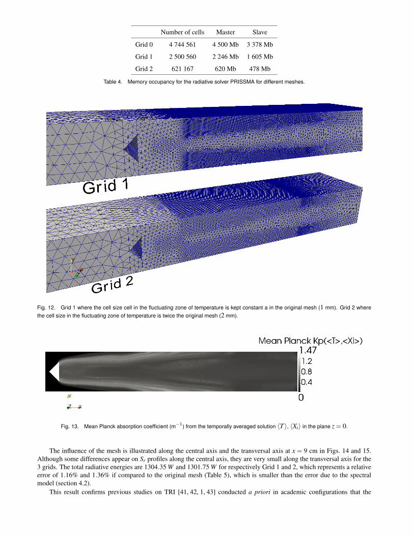
To evaluate the dependence of the accuracy of the solution on the mesh resolution , 3 grids have been tested. The originalmesh (Grid 0) contains 4 744 561 cells with a cell size of 1 mm close to the flame holder. Starting from Grid 0 and using theaverage temperature fields, two meshes have been built, shown in Fig. 12. The grids keep the cells as small as possible wheretemperature RMS (Root Main Square) is important (Fig. 11), while the size of the cells is increased to about 1 cm in thefresh gases zone where there is no absorption (only the absorption of CO2, H2O, CO are considered here). Grid 1 contains

0,05 0,1 0,15 0,2 0,25Central axis x (m)

1,4e+06

1,6e+06

1,8e+06

2e+06

2,2e+06

2,4e+06

Rad

iativ

e So

urce

term

Sr (W

/m3 )

Sr(T(t1),Xk(t1))Sr(T(t1+100it),Xk(t1+100it))Sr(<T>100it,<Xk>100it)

Fig. 10. Radiative source term along the central axis, calculated at t1, t1 +100it and with the time averaged variables over 100 iterations.

Fig. 11. Mean and RMS temperature fields in y = 0 plane.

2 500 560 cells, and has the same cell size as Grid 0 (1 mm) in the temperature fluctuating zone. Grid 2 contains 621 167cells and has cells twice the size of Grid 0 (2 mm) in the temperature fluctuating zone. The associated memory occupancy isgiven in Table 4 : it decreases linearly with the cell number.

Al grids must guarantee optically thin cells as required by the Diamond Mean Flux Scheme (DMFS) used in PRISSMA[2] to avoid numerical scattering, so-called “false-scattering”. Using the mean Planck absorption coefficient to a criterionfor the maximal cell size as : κP∆x ≤ 0.1. Fig. 13 shows κP for the mean solution in the range [0;1.47]m−1 which gives amaximum cell size of 7cm, far above the cell size in all grids.

Number of cells Master Slave

Grid 0 4 744 561 4 500 Mb 3 378 Mb

Grid 1 2 500 560 2 246 Mb 1 605 Mb

Grid 2 621 167 620 Mb 478 Mb

Table 4. Memory occupancy for the radiative solver PRISSMA for different meshes.

Fig. 12. Grid 1 where the cell size cell in the fluctuating zone of temperature is kept constant a in the original mesh (1 mm). Grid 2 wherethe cell size in the fluctuating zone of temperature is twice the original mesh (2 mm).

Fig. 13. Mean Planck absorption coefficient (m−1) from the temporally averaged solution 〈T 〉, 〈Xi〉 in the plane z = 0.

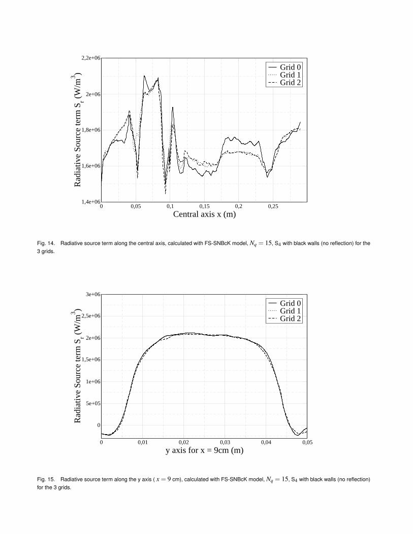
The influence of the mesh is illustrated along the central axis and the transversal axis at x = 9 cm in Figs. 14 and 15.Although some differences appear on Sr profiles along the central axis, they are very small along the transversal axis for the3 grids. The total radiative energies are 1304.35 W and 1301.75 W for respectively Grid 1 and 2, which represents a relativeerror of 1.16% and 1.36% if compared to the original mesh (Table 5), which is smaller than the error due to the spectralmodel (section 4.2).

This result confirms previous studies on TRI [41, 42, 1, 43] conducted a priori in academic configurations that the

0 0,05 0,1 0,15 0,2 0,25Central axis x (m)

1,4e+06

1,6e+06

1,8e+06

2e+06

2,2e+06

Rad

iativ

e So

urce

term

Sr (W

/m3 )

Grid 0Grid 1Grid 2

Fig. 14. Radiative source term along the central axis, calculated with FS-SNBcK model, Nq = 15, S4 with black walls (no reflection) for the3 grids.

0 0,01 0,02 0,03 0,04 0,05y axis for x = 9cm (m)

0

5e+05

1e+06

1,5e+06

2e+06

2,5e+06

3e+06

Rad

iativ

e So

urce

term

Sr (W

/m3 )

Grid 0Grid 1Grid 2

Fig. 15. Radiative source term along the y axis ( x = 9 cm), calculated with FS-SNBcK model, Nq = 15, S4 with black walls (no reflection)for the 3 grids.

Quadrature Total radiative εtot Errors on central profile (%)

energy (W) (%) ε σ

Grid 0 1 326.31 – – –

Grid 1 1 304.35 1.16 2.39 1.77

Grid 2 1 301.75 1.36 2.46 1.52

Table 5. Accuracy on the total radiative energy εtot and on the radiative source term along the central axis ε, σ of grid resolution on theradiative solution using FS-SNBck15, the relative error is calculated against Grid 0 solution.

influence on the radiation of subgrid scale fluctuation is small. Here the increase of the mesh size, between Grid 0 and 2, isequivalent to a spatial filtering with a filter size from 2∆xLES to 10∆xLES. As ignoring the fluctuations smaller than 2∆xLESgive a maximal error of 1.36%, it is possible to conclude a posteriori no subgrid scale model is required for radiation in LEScontext.

6 Influence of the boundary conditions : reflective wallsFrom a radiative point of view, walls are characterized by a temperature and an emissivity. The ceramic wall emissivity

is ε = 0.91 [3]. The flame holder emissivity is taken from for a stainless steels lightly oxidized at 1000 K, ε = 0.4 [3]. Theinlet, outlet and the atmosphere are assumed to be black enclosures (i.e. all incident radiation is absorbed).

Quartz windows are semi-transparent, i.e. their emissivity is a function of the wavelength (Fig. 16). This is a particularityof the experimental configuration as in a real combustor there are no transparent walls. The quartz spectral emissivity shownin Fig. 16 [3] was provided by the manufacturer for the interval [0.5;4.5 µm] and results from an emissivity calculation basedon the complex index of the medium [44] for the interval [4.5;15 µm]. It is assumed to be 1 in the interval [15;68 µm]. Todescribe the quartz emissivity in global spectral models the mean emissivity (weighted by the Planck function) over the fullspectrum is calculated. Using the temperature of 300 K, the mean quartz emissivity is ε = 0.879 even for the SNBcK case.

0,5 1 2 4 8 16 32 64Wavelength λ (µm)

0

0,2

0,4

0,6

0,8

1

Emis

sivi

ty

Quartz emissivityin the range λ=[0.5;68µm]

Fig. 16. Quartz spectral emissivity.

Spectral model Total radiative εtot

energy (W) (%)

SNBcK 1331.47 4.69

WSGG 900.92 4.94

FS-SNBcK15 1254.49 4.93

FS-SNBcK15, Tab. 1273.82 4.35

Table 6. Relative difference εtot on the total radiative energy for different spectral models compared to the cases without reflection.

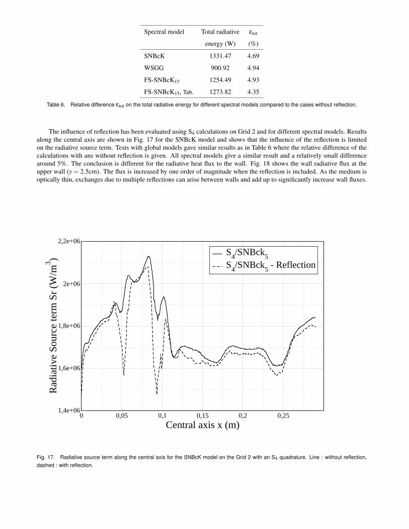
The influence of reflection has been evaluated using S4 calculations on Grid 2 and for different spectral models. Resultsalong the central axis are shown in Fig. 17 for the SNBcK model and shows that the influence of the reflection is limitedon the radiative source term. Tests with global models gave similar results as in Table 6 where the relative difference of thecalculations with ans without reflection is given. All spectral models give a similar result and a relatively small differencearound 5%. The conclusion is different for the radiative heat flux to the wall. Fig. 18 shows the wall radiative flux at theupper wall (y = 2.5cm). The flux is increased by one order of magnitude when the reflection is included. As the medium isoptically thin, exchanges due to multiple reflections can arise between walls and add up to significantly increase wall fluxes.

0 0,05 0,1 0,15 0,2 0,25Central axis x (m)

1,4e+06

1,6e+06

1,8e+06

2e+06

2,2e+06

Rad

iativ

e So

urce

term

Sr (

W/m

3 ) S4/SNBck5S4/SNBck5 - Reflection

Fig. 17. Radiative source term along the central axis for the SNBcK model on the Grid 2 with an S4 quadrature. Line : without reflection,dashed : with reflection.

0 0,05 0,1 0,15 0,2 0,25x axis for the upper wall for y = 2.5cm (m)

0

1e+05

2e+05

3e+05

4e+05

5e+05

6e+05W

all H

eat F

lux

Qw

(W/m

2 )

S4/SNBck5S4/SNBck5 - Reflection

Fig. 18. Wall radiative flux along the x axis at y = 2.5 cm et z = 0 (quartz wall) for the SNBcK model on Grid 2 with an S4 quadrature.Line : without reflection, dashed : with reflection.

7 Summary of calculation time and accuracyThe performance in terms of accuracy and computing time of the radiative solver with all possible models and dis-

cretizations are summarized in Table 7. The calculation times is given for a parallel calculation on 24 Intel(R) Xeon(R) CPU@ 2.66 GHz processors.

The radiative calculation time is split into 2 contributions, corresponding to spectral calculations (calculation of the ab-sorption coefficient) and the geometrical calculations (integration of the RTE). The total time is the sum of both contributionsplus the communication time and data I/O time.

As the absorption coefficients are functions of local variables the spectral calculation is parallelized with a domaindecomposition method. WSGG and tabulated FS-SNBcK models use tabulated absorption coefficients the spectral time isnegligible for these cases. The spectral calculation time is longer for the FS-SNBcK model than the SNBcK model becauseof the numerical inversion of the full spectrum cumulative function [34].

The geometrical time for all global models is much reduced compared to the SNBcK because the decrease of the numberof resolutions of the RTE. Because of prohibitive CPU time, the LC11/SNBcK5 and S4/SNBcK5 with reflection calculationtimes are only estimated. Grid reduction is also very efficient in reducing the calculation time linearly with the number ofcells.

Finally, including reflection increases the geometrical time increases by a factor 3 to 4 (the resolution of the RTE hasbeen iterated 3 or 4 times to reach the convergence). Obviously global models should be used if the reflection is consideredas the geometrical time is small compared to the use of SNBcK.

The accuracy of the solution is estimated from the total radiative energy calculated in Tables 2, 3 and 5. The total erroris the sum of the errors linked to spectral model, angular quadrature and grid resolution. As an example, the error of thesolution WSGG/S4 on the mesh 1 is : 32.57 (Tab. 3) +1.16 (Tab. 5) +0.5 (Tab. 2) = 34.23%. Solutions with an error above10% are considered unacceptable. Clearly all WSGG calculations are not sufficiently accurate, while all SNBcK are alwaysexcellent even on the coarser mesh and FS-SNBcK15 are good on all meshes.

Spectral Total PRISSMA/AVBP Cumulated

Quadrature time (s) time (s) time (s) (TTGC)

502,84 494,41 -

502,84 125,37 0,5

502,84 -

502,84 371,40 0,5

876,05 23,17 5,53

219,01 20,06 6,03

21,25 200,47 239,90 1,13 4,59

146,01 10,38 9,15

102,21 7,21 10,16

WSGG 6,19 39,61 89,27 0,42 33,07

107,67 9,02 7,19

WSGG 3,26 21,93 41,63 0,20 34,23

442,61 56,60 1,86

395,84 25,75 482,30 2,27 7,39

5,32 25,55 36,76 0,17 5,95

WSGG 0,81 5,19 9,70 0,05 34,43

469,47 220,72 1,86

393,05 46,71 692,41 3,25 7,39

2,25 66,10 132,88 0,62 5,95

0,81 12,71 17,84 0,08 34,43

AVBP Ratio

106,45 1 Acceptable precision

TTGC 212,89 1,9 Unacceptable precision

7,64 LC11 : 96 directions

Number of processors: 24 S4 : 24 directions

Grid Angular Spectral Model Geometrical

(Reflection) errors (%)

Grid 0 LC11

SNBck5 (estimated) 104 753,64 105 256,49

Grid 0 S4

SNBck5 26 188,41 26 691,26

Grid 0 LC11

SNBck5 – Reflection (estimated) 314 260,93 314 763,78 1 478,52

Grid 0 S4

SNBck5 – Reflection (estimated) 78 565,23 79 068,08

Grid 0 LC11

FS-SNBck15 4 022,75 4 931,88

Grid 0 S4

FS-SNBck15 4 022,75 4 269,89

Grid 0 S4

FS-SNBck15

Tab.

Grid 0 S4

FS-SNBck10 2 062,87 2 208,88

Grid 0 S4

FS-SNBck7 1 433,50 1 535,70

Grid 0 S4

Grid 1 S4

FS-SNBck15 1 572,41 1 919,53

Grid 1 S4

Grid 2 S4

SNBck5 4 863,08 12 049,66

Grid 2 S4

FS-SNBck15

Grid 2 S4

FS-SNBck15

Tab.

Grid 2 S4

Grid 2 S4

SNBck5 – Reflection 20 903,66 46 990,05

Grid 2 S4

FS-SNBck15

– Reflection

Grid 2 S4

FS-SNBck15

Tab. – Reflection

Grid 2 S4 WSGG – Reflection

Time for Nit=100 iterations # cells Reference solution

Lax-Wendroff 4 744 561

2 500 560

621 167

Table 7. Radiative calculation times for set of parameters, obtained on 24 processors Intel(R) Xeon(R) CPU @ 2.66 GHz.

In the PCS coupling (section 3.1), the radiation calculation time must be compared to the combustion CPU time for 100iterations over 24 processors. This time is 106 s with the 2nd order spatial scheme (Lax-Wendroff) and 212 s with the 3rd

order spatial scheme (TTGC) in the AVBP solver. In the case where the same number of processors is allocated to the fluidand the radiation solver the ratio of calculation times PRISSMA/AVBP (for the TTGC scheme) is given in the 7th columnof Table 7. These ratio are sorted by decreasing in Fig. 19. Good solution correspond to a ratio less than 1, meaning that acoupled simulation cost or less than CPU of uncoupled calculation.

The reference solutions reach ratios up to 1 400. The ratio for S4/SNBcK on Grid 0 without reflection is 125 which isstill unacceptable. The tabulated FS-SNBck15/S4 calculation on Grid 2 gives an efficient ratio of 0.17.

The tabulated FS-SNBck15/S4 on Grid 2 with reflection is the optimum case, ensuring both rapidity and accuracy.The error on the total radiative energy is 5.95% which is acceptable in comparison to the precision of LES calculations.This optimum demonstrated that using global spectral models with reflection and sufficient number of discrete directions ismore accurate than narrow band models where the high CPU cost imposes to neglect reflection or decrease the number ofdirections.

8 ConclusionWith the objective of coupled combustion-radiation simulations, a premixed turbulent flame has been studied from a

radiative point of view to evaluate the efficiency and accuracy of the radiative solver.A study of the models and discretization used in the radiative solver have been conduced on the angular quadrature, the

spectral model and the spatial/temporal discretization. It has been demonstrated the spectral model is the most important

Fig. 19. Ratio of calculation times PRISSMA/AVBP for the different models and discretisations of the radiative solver.

parameter for combustion applications both for accuracy and CPU time.The systematic comparison of the different parameters and choice of radiative models in terms of precision and cost

demonstrate that a tabulated FS-SNBcK15/S4 on the coarsest grid and including reflection is the optimal combination. Theradiative calculation time is then 350 times shorter than a SNBcK/S4 calculation on the original mesh, and introduces anerror less than 6%. With this model it is possible to obtain a radiative solution within a time 0.6 times shorter than 100combustion iterations, the objective of reaching a CPU time ratio PRISSMA/AVBP less than one.

A mesh reduction has been applied to reduce the radiative calculation time and the memory occupancy of the radiativesolver following the criterion of temperature fluctuations. It can be concluded that the radiative grid is larger than the fluidmesh. Mesh convergence confirms a posteriori the small influence of the LES subgrid scale fluctuations on radiation, andthere is no need for subgrid models for radiation in LES.

An other important result is that it is possible to take into account reflection if a global spectral model is used. If theinfluence of reflection on the radiative source term is small, it remains very important for the radiative wall fluxes.

This work constitutes a first step toward coupled CFD-radiation simulations selecting the optimal methodology basedon systematic comparisons. Coupled simulation are underway and the analysis of the influence of radiation on combustionwill be discussed in a future paper.

References[1] Coelho, P. J., 2009. “Approximate solutions of the filtered radiative transfer equation in large eddy simulations of

turbulent reactive flows”. Combustion and Flame, 156(5), May, pp. 1099–1110. 1, 11, 14[2] Joseph, D., 2004. “Modelisation des transferts radiatifs en combustion par methode aux ordonnees discretes sur des

maillages non structures tridimensionnels”. PhD thesis, Institut National Polytechnique de Toulouse. 1, 6, 13[3] dos Santos, R. G., 2007. “Large eddy simulation of turbulent combustion including radiative heat transfer”. PhD thesis,

EM2C. 1, 2, 4, 5, 8, 16[4] Sagaut, P., 1998. Introduction a la simulation des grandes echelles pour les ecoulements de fluide incompressible.

Mathematiques & Applications, Vol. 30. 1[5] Poinsot, T., and Veynante, D., 2001. Theorical and Numerical Combustion. Edwards. 1

[6] Boileau, M., Staffelbach, G., Cuenot, B., Poinsot, T., and Berat, C., 2008. “LES of an ignition sequence in a gas turbineengine”. Combustion and Flame, 154(1-2), pp. 2–22. 1

[7] Nottin, C., Knikker, R., Boger, M., and Veynante, D., 2000. “Large eddy simulations of an acoustically excited turbulentpremixed flame”. Symposium (International) on Combustion, 28(1), pp. 67–73. 1, 2

[8] Roux, A., Gicquel, L., Sommerer, Y., and Poinsot, T., 2008. “Large eddy simulation of mean and oscillating flow inside-dump ramjet combustor”. Combustion and Flame, 152(1-2), pp. 154–176. 1

[9] Boudier, G., Gicquel, L., and Poinsot, T., 2008. “Effects of mesh resolution on large eddy simulation of reacting flowsin complex geometry combustors”. Combustion and Flame, 155, pp. 196–214. 1

[10] Coelho, P. J., 2007. “Numerical simulation of the interaction between turbulence and radiation in reactive flows”.Progress in Energy and Combustion Science, 33(4), Aug., pp. 311–383. 2, 11

[11] Desjardin, P. E., and Frankel, S. H., 1999. “Two-dimensional large eddy simulation of soot formation in the near-fieldof a strongly radiating nonpremixed acetylene-air turbulent jet flame”. Combustion and flame, 119(1-2), pp. 121–132.2

[12] Jones, W., and Paul, M., 2005. “Combination of DOM with LES in a gas turbine combustor”. International Journal ofEngineering Science, 43(5-6), Mar., pp. 379–397. 2

[13] Joseph, D., Hafi, M. E., Fournier, R., and Cuenot, B., 2005. “Comparison of three spatial differencing schemes indiscrete ordinates method using three-dimensional unstructured meshes”. International Journal of Thermal Sciences,44(9), Sept., pp. 851–864. 2, 6

[14] Joseph, D., Perez, P., Hafi, M. E., and Cuenot, B., 2009. “Discrete Ordinates and Monte-Carlo Methods for radiativetransfer simulation applied to computational fluid dynamics combustion modeling”. Journal of Heat Transfer, 131(5),May, pp. 052701–9. 2, 6, 9

[15] dos Santos, R. G., Lecanu, M., Ducruix, S., Gicquel, O., Iacona, E., and Veynante, D., 2008. “Coupled large eddysimulations of turbulent combustion and radiative heat transfer”. Combustion and Flame, 152(3), Feb., pp. 387–400.2, 5, 8

[16] Knikker, R., Veynante, D., Rolon, J., and Meneveau, C., 2000. “Planar laser-induced fluorescence in a turbulentpremixed flame to analyze Large Eddy Simulation models”. In Proceedings of the 10th international Symposium onApplications of Laser Techniques to Fluid Mechanics. 2

[17] Knikker, R., Veynante, D., and Meneveau, C., 2002. “A priori testing of a similarity model for large eddysimulationsof turbulent premixed combustion”. Proceedings of the Combustion Institute, 29(2), pp. 2105–2111. 2

[18] Colin, O., and Rudgyard, M., 2000. “Development of high-order Taylor-Galerkin schemes for LES”. Journal ofComputational Physics, 162(2), pp. 338–371. 3, 7

[19] Ducros, F., Nicoud, F., and Poinsot, T., 1998. “Wall-adapting local eddy-viscosity models for simulations in complexgeometries”. In ICFD, B. M. J., ed., pp. 293–300. 3

[20] Nicoud, F., and Ducros, F., 1999. “Subgrid-scale stress modelling based on the square of the velocity gradient tensor”.Flow, Turbulence and Combustion, 62(3), pp. 183–200. 3

[21] Colin, O., Ducros, F., Veynante, D., and Poinsot, T., 2000. “A thickened flame model for large eddy simulations ofturbulent premixed combustion part2”. Physics of Fluids, 12(7), pp. 1843–1863. 3

[22] Selle, L., Lartigue, G., Poinsot, T., Koch, R., Schildmacher, K.-U., Krebs, W., Prade, B., Kaufmann, P., and Vey-nante, D., 2004. “Compressible Large-Eddy Simulation of turbulent combustion in complex geometry on unstructuredmeshes”. Combustion and Flame, 137(4), pp. 489–505. 3

[23] Poinsot, T., and Lele, S., 1992. “Boundary conditions for direct simulations of compressible viscous flows”. Journalof Computational Physics, vol.101(1), pp. 104–129. 3

[24] Amaya, J., 2010. “Unsteady coupled convection, conduction and radiation simulations on parallel architectures forcombustion applications”. PhD thesis, CERFACS. 4

[25] Poitou, D., 2009. “Modelisation du rayonnement dans la simulation aux grandes echelles de la combustion turbulente”.PhD thesis, Institut National Polytechnique de Toulouse, Decembre. 5, 6, 11

[26] Joseph, D., Coelho, P. J., Cuenot, B., and Hafi, M. E., 2003. “Application of the discrete ordinates method to greymedia in complex geometries using 3-dimensional unstructured meshes”. In Eurotherm73 on Computationnal ThermalRadiation in Participating Media, Vol. 11, Eurotherm series, pp. 97–106. 6

[27] Jensen, K. A., Ripoll, J., Wray, A., Joseph, D., and Hafi, M. E., 2007. “On various modeling approaches to radiativeheat transfer in pool fires”. Combustion and Flame, 148(4), Mar., pp. 263–279. 6, 9

[28] Truelove, J. S., 1987. Discrete-ordinate solutions of the radiation transport equation. 6[29] Goutiere, V., Liu, F., and Charette, A., 2000. “An assessment of real-gas modelling in 2D enclosures”. Journal of

Quantitative Spectroscopy and Radiative Transfer, 64, Feb., pp. 299–326. 6[30] Goutiere, V., Charette, A., and Kiss, L., 2002. “Comparative performance of non-gray gas modeling techniques”.

Numerical Heat Transfer Part B: Fundamentals, 41, Mar., pp. 361–381. 6[31] Soufiani, A., and Taine, J., 1997. “High temperature gas radiative propriety parameters of statistical narrow-band model

for H2O, CO2 and CO and correlated-k model for H2O and CO2”. Technical note in International Journal of Heat and

mass transfer, 40, pp. 987–991. 6[32] Soufiani, A., and Djavdan, E., 1994. “A comparison between weighted sum of gray gases and statistical narrow-band

radiation models for combustion applications”. Combustion and Flame, 97(2), pp. 240 – 250. 6[33] Liu, F., Yang, M., Smallwood, G., and Zhang, H., 2004. “Evaluation of the SNB based full-spectrum CK method for

thermal radiation calculations in CO2−H2O mixtures”. In Proceedings of ICHMT. 6[34] Poitou, D., Amaya, J., Bushan Singh, C., Joseph, D., Hafi, M. E., and Cuenot, B., 2009. “Validity limits for the global

model FS-SNBcK for combustion applications”. In Proceedings of Eurotherm83 – Computational Thermal Radiationin Participating Media III. 6, 7, 10, 18

[35] Amaya, J., Cabrit, O., Poitou, D., Cuenot, B., and Hafi, M. E., 2010. “Unsteady coupling of Navier-Stokes and radiativeheat transfer solvers applied to an anisothermal multicomponent turbulent channel flow”. Journal of QuantitativeSpectroscopy and Radiative Transfer, 111(2), pp. 295–301. 7

[36] Duchaine, F., Corpron, A., Pons, L., Moureau, V., Nicoud, F., and Poinsot, T., 2009. “Development and assessmentof a coupled strategy for conjugate heat transfer with Large Eddy Simulation. Application to a cooled turbine blade”.International Journal of Heat and Mass Transfer, submitted. 7

[37] Leacanu, M., 2005. “Couplage multi-physique combustion turbulente - rayonnement - cinetique chimique”. PhD thesis,Ecole centrale Paris. 8

[38] Wang, Y., 2005. “Direct numerical simulation of non-premixed combustion with soot and thermal radiation”. PhDthesis, University of Maryland. 8

[39] Staffelbach, G., Gicquel, L. Y. M., and Poinsot, T., 2007. Highly Parallel Large Eddy Simulations of MultiburnerConfigurations in Industrial Gas Turbines, Vol. Complex Effects in LES. pp. 325–336. Lecture Notes in ComputationalScience and Engineering. 8

[40] Zhang, J., Gicquel, O., Veynante, D., and Taine, J. “Monte carlo method of radiative transfer applied to a turbulentflame modeling with LES”. Comptes Rendus Mecanique, 337(6-7), pp. 539–549. 10

[41] Poitou, D., Hafi, M. E., and Cuenot, B., 2007. “Diagnosis of Turbulence Radiation Interaction in turbulent flames andimplications for modeling in Large Eddy Simulation”. Turkish Journal of Engineering and Environmental Sciences,31, pp. 371–381. 11, 12, 14

[42] Roger, M., Silva, C. B. D., and Coelho, P. J., 2009. “Analysis of the turbulence-radiation interactions for Large EddySimulations of turbulent flows”. International Journal of Heat and Mass Transfer, 52(9-10), pp. 2243 – 2254. 11, 14

[43] Roger, M., Coelho, P. J., and da Silva, C. B., 2010. “The influence of the non-resolved scales of thermal radiation inLarge Eddy Simulation of turbulent flows: A fundamental study”. International Journal of Heat and Mass Transfer,53(13-14), pp. 2897–2907. 11, 14

[44] Palik, E. D., and Ghosh, G., 1998. Handbook of optical constants of solids. Academic Press. 16