72
Analysis of Signalized Intersections

Analysis of Signalized Intersections

2
What is Intersection analysis
Inverse application of the signal timing design In signal timing design, green times
are estimated to provide necessary capacity
In intersection analysis, signal timing is known and used to estimate the existing capacity

Two methods
Critical Movement Approach Apply adjustment factors to the
demand volume
HCM Methodology Saturation flow rates are reduced to
reflect non-ideal prevailing conditions
3

4
Steps for Critical Movement Approach
1. Identify the lane geometry and use 2. Identify hourly demand volumes 3. Specify the signal timing 4. Convert demand volumes to equivalent passenger-car
Volumes 5. Convert passenger-car equivalents to through-car
equivalents 6. Convert Through-car equivalents under prevailing
conditions to though-car equivalents under ideal conditions 7. Assign lane flow rates 8. Find critical-lane flows 9. Determine capacity and v/c ratios 10. Determine delay and level of service

5
1. Proportion of heavy vehicles 2. Proportion of local buses 3. Lane widths 4. Approach grade 5. Parking conditions on approach 6. Pedestrian interference levels
Identify hourly demand volumes

6
1. Proportion of heavy vehicles 2. Proportion of local buses 3. Lane widths 4. Approach grade 5. Parking conditions on approach 6. Pedestrian interference levels
Identify hourly demand volumes

Identify signal timings
7
1 2g G y ar l l= + + − −Effective green time Actual green time Actual yellow time Actual all-red time Start-up lost time Clearance lost time
gGy
ar1l2l

Convert Demand Volume to Equivalent Passenger Car Volume
8
(1 )pc HV HV LB LB HV LBV VP E VP E V P P= + + − −

Passenger-car Equivalents for Local Buses (Stop in Travel Lane)
9

Passenger-car Equivalents for Local Buses (Stop in Parking Lane)
10

Convert Passenger-Car Equivalent to Through-Car Equivalent
11
Left Turn Vehicles Protected left turns = 1.05 Permitted depends on opposing flow and
number of opposing lanes Right Turn Vehicles Depends on the pedestrian volume in
conflicting crosswalk

Through Car Equivalent for Left-Turning Vehicles
12

Through Car Equivalent for Right-Turning Vehicles
13
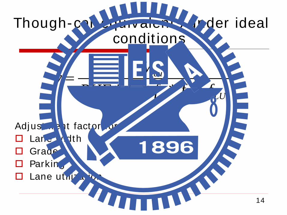
Though-car equivalents under ideal conditions
14
* * * *tcu
w g p LU
VvPHF f f f f
=
Adjustment factor for: Lane width Grade Parking Lane utilization

Lane Width Adjustment
15

Grade Adjustment
16
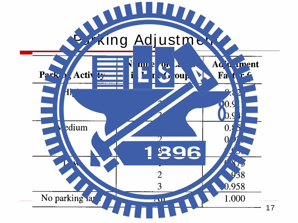
Parking Adjustment
17

Lane Utilization Adjustment
18

Assign Lane Flow Rates
19
Where a separate LT lane exist, assign all LT tcus to this lane group. If more than one lane exists, divide the tcu/h equally among the lanes
Where a separate RT lane exist, assign all RT tcus to this lane group. If more than one lane exists, divide the tcu/h equally among the lanes
For all mixed lane group(LT/TH/RH, LT/TH, TH/RT)divide the total tcu/h equally among all lanes, except that all LT tcus must be in the LH lane and all RT tcus in RH lane

Find Critical Lane Flow Rates for Each Signal Phase
20
From A1 to A3 Ring 1 148+420=568 Ring 2 203+330=533
Maximum = 568
From B1 to B3 Ring 1 120+380=500 Ring 2 220+250=570
Maximum = 570 1138

Capacity and v/c Ratio
21
From A1 to A3 Ring 1 148+420=568 Ring 2 203+330=533
Maximum = 568
From B1 to B3 Ring 1 120+380=500 Ring 2 220+250=570
Maximum = 570 1138
1900( / )i ic g C=
11900( / )
n
SUM ii
c g C=
= ∑/i i iX v c=
1/
n
c i ii
X v c=
=∑

Delay and Level of Service
22
1 2*i i id d PF d= +
Approach delay for lane group i Uniform delay for lane group I Overflow plus random delay for lane group i Progression adjustment factor
id1id2id
PF

Uniform Delay and Overflow delay
23
2
10.5 [1 ( / )]
1 [min(1, )*( / )]i
ii i
C g CdX g C−
=−
22
16225[( 1) ( 1) ]ii i i
i i
Xd X Xc N
= − + − +
Uniform Delay:
Overflow Delay:

Progression Factor
24

Level of Service
25

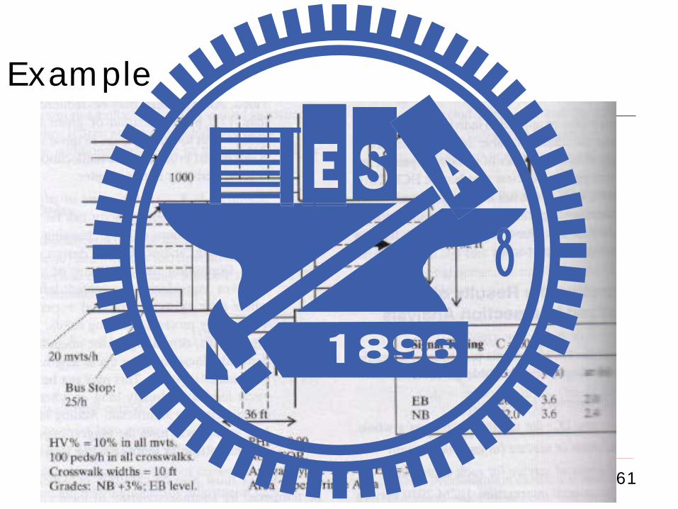
Example
26

Step 1 and 2: Geometry and volume
27

Step 3:Signal Phase
28

Step 4: Conversions to Equivalent Passenger Car Flow
29
EB Through movement 1100 veh/h, 10% heavy vehicle and 20 buses/hour Heavy=1100*10%*2.0=220 Bus=20*3.1=62 Passenger_car=1100*(1-10%)-20=970 Total=Heavy+Bus+Passenger_car=1252

Step 4: Conversions to Through-Car Equivalent
30
EB left turn Protected, equivalent=1.05
NB left turn One-way street, No conflicting through Go through pedestrian crosswalk Pedestrian volume 100 ped/h Treated like right turn, equivalent=1.21

Step 5: Conversions to Equivalent Under Ideal Condition
31
No parking, fp=1.0 EB lane width is 11 feet, fw=0.97 EB Through has two lanes f=0.952


Step 6: Assign Flow to Lanes
33
WB approach 183 tch/h for right turn and 1242 for
through Total 1424 uniformly split between two
lanes Leftmost lane 712 through only Rightmost lane carries 183 right turn and
1241-712=529 through
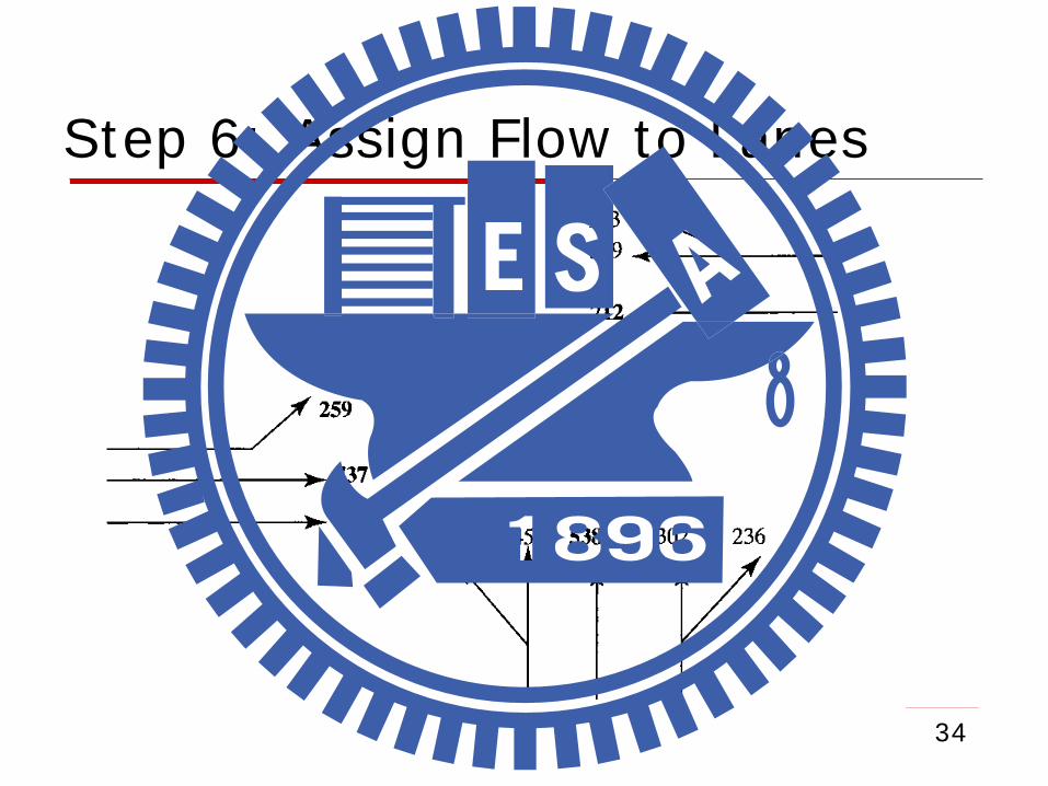
Step 6: Assign Flow to Lanes
34

Step 7: Critical Volume
35

Step 8: Capacity and v/c ratio
36

Step 8: Capacity and v/c ratio
37

Step 9: Delay and LOS
38
Uniform Delay:

Step 9: Delay and LOS
39
Overflow Delay:

Step 9: Delay and LOS
40
Total Delay = d1*PF+d2:
41
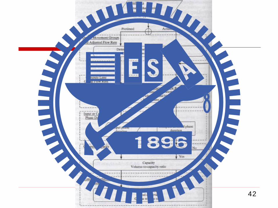
Steps for HCM Approach
1. Input data
2. Define movement groups and adjusted flow rate
3. compute lane group flow rate
4. input or compute phase duration
5. Compute capacity
6. Compute delays and LOS
42

43
Step 2: Movement and lane groups
44
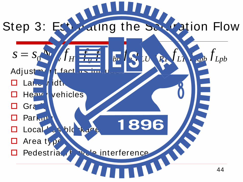
Step 3: Estimating the Saturation Flow
Adjustment factors include: Lane width Heavy vehicles Grade Parking Local bus blockage Area type Pedestrian/bicycle interference
0 w HV g p bb a LU RT LT Rpb Lpbs s Nf f f f f f f f f f f=

45
Adjustment for Lane Width
Lanes width less than 10 ft Lane width between 10 and 12.9 ft Lane width larger than 12.9 ft
0.96wf =
1.0wf =
1.04wf =
46
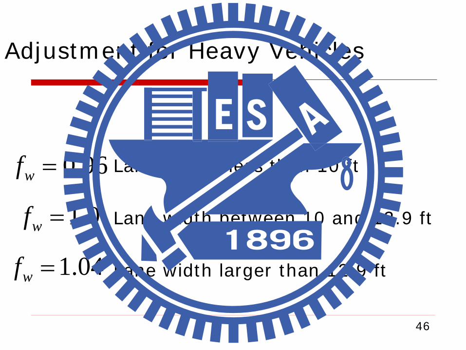
Adjustment for Heavy Vehicles
Lanes width less than 10 ft Lane width between 10 and 12.9 ft Lane width larger than 12.9 ft
0.96wf =
1.0wf =
1.04wf =
47
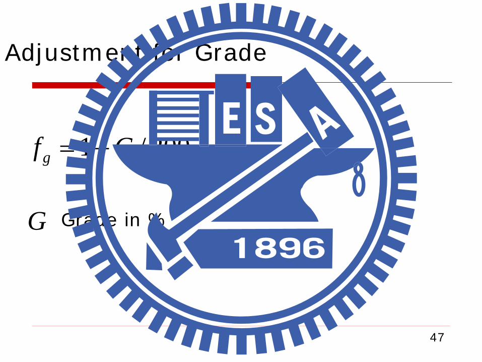
Adjustment for Grade
1 / 200gf G= −
G Grade in %

48
Adjustment for Parking
180.9 ( )3600
mNP = − ( 1)p
N PfN− +
=
180.1 ( )3600 0.05
m
p
NNf
N
− −= ≥
49
Adjustment for Local Bus Blockage
14.41.0 ( )3600
BNB = − ( 1)bb
N BfN− +
=
14.4( )3600 0.05
B
p
NNf
N
−= ≥

50
Adjustment for Type of Area
0.9af =CBD location:
Other location: 1.0af =

51
Adjustment for Lane Utilization
1
gLU
g
vf
v N=
Demand flow rate for the lane group gv
1gv Demand flow rate for highest lane volume
N Number of lanes in the lane group
52
Adjustment for Protected Turns
0.85RTf = For exclusive RT lane
0.95LTf = For protected LT lane

53
Adjustment for Pedestrian and Bicycle Interference with Turns
Estimate Pedestrian Flow Rate During Green Phase Estimate the Average Pedestrian Occupancy in the Conflict
Zone Estimate the Bicycle Flow Rate During the Green Phase Estimate the Average Bicycle Occupancy in the Conflict
Zone Estimate the Conflict Zone Occupancy Estimate the Unblocked Portion of the Phase Determine Adjustment Factors

54
Step 4: Determine Lane Group Capacities and v/c Ratios
Capacity of a lane group
v/c ratio of a lane group
Critical v/c ratio for intersection
( / )i i ic s g C=
( / )( / )
i ii
i i
v v sXc g C
= =
maxmin
max
( / ) *( )iC c
i
CX v sC L
=−∑
55
Step 5: Critical Lane Group Identification

56
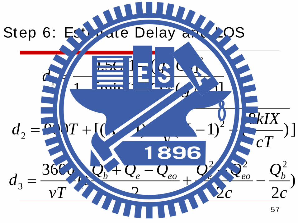
Step 6: Estimate Delay and LOS
Uniform Delay
Incremental Delay
Additional Delay Per Vehicle Due to Queue
1 2 3d d d d= + +
1d
2d
3d
57
Step 6: Estimate Delay and LOS
2
10.5 [1 ( / )]
1 [min(1, )*( / )]C g Cd
X g C−
=−
22
8900 [( 1) ( 1) ( )]kIXd T X XcT
= + − + − +
2 2 2
33600 ( )
2 2 2b e eo e eo bQ Q Q Q Q Qd t
vT c c+ − −
= + −

58
Step 6: Aggregate Delay
i ii
Ai
i
d vd
v=∑∑
A AA
IA
i
d vd
v=∑∑

59
Step 7: Interpret the Results
v/c ratios X for every lane group Critical v/c ratio X for the intersection Delays and LOS for each lane group Delays and LOS for each approach Delays for overall intersection

60
Step 7: Interpret the Results
Scenario I: Xc<1.0,all Xi<1.0, no capacity deficiency Scenario II;
Xc<1.0,some Xi>1.0, reallocation of green time needed
Scenaio III: Xc>1.0,some or all Xi>1.0, change of phase plan, cycle length, or physical design is needed
61
Example

62
Volume Adjustment

63
Saturation Flow Rate Estimation
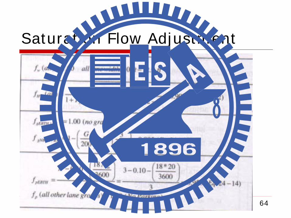
Saturation Flow Adjustment
64

Saturation Flow Adjustment
65

Saturation Flow Adjustment
66

Saturation Flow Adjustment
67

Saturation Flow Adjustment
68

Capacity Analysis
69
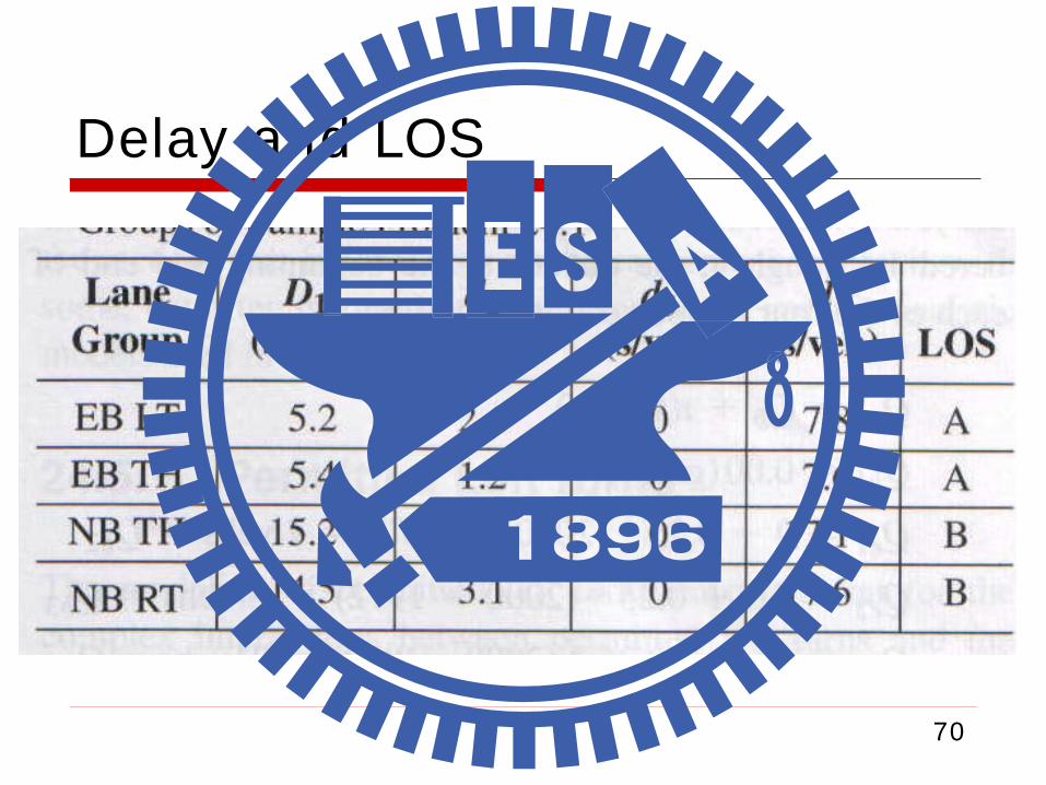
Delay and LOS
70

What is the result if applying HCM to the former Critical Movement analysis example?
71

72


