ANALYSIS OF SOURCE LOCATION ALGORITHMSPart II: Iterative methods
MAOCHEN GEPennsylvania State University, University Park PA 16802
Abstract
Iterative algorithms are of particular importance in source location as they provide a muchmore flexible means to solve nonlinear equations, which is essential in order to deal with a widerange of practical problems. The most important iterative algorithms are Geiger’s method and theSimplex method. This article provides an overview of iterative algorithms as well as an in-depthanalysis of several major methods.
1. Introduction
In Part I, we discussed the non-iterative location methods. A restriction that severely limitsthe application of these methods is the assumption of a single velocity for all channels. This as-sumption is not arbitrary or just for convenience; it is necessary in order to keep the source loca-tion equations in the simplest form so that they can be solved non-iteratively. In other words, theassumption is a reflection of an inherent difficulty associated with non-iterative location meth-ods. If a single velocity model is not suitable, as in most cases, we have to turn to an iterativemethod.
While the associated searching strategies may vary significantly, iterative methods in generalrefer to those algorithms that start from an initial solution, commonly called a guess or trial solu-tion. This trial solution is tested by the given conditions, and then updated by the predefinedschemes, which subsequently forms a new trial solution. Therefore, iterative methods, in es-sence, are a process of testing and updating trial solutions.
An iterative method is distinguished by its updating scheme, which determines its efficiencyas well as its other major characters. While there are many different schemes, the ones that aretruly significant both theoretically and practically are few for the purpose of source location. Theobject of this article is to provide an in-depth analysis of these methods. But first we will give abrief review on the basic searching approaches.
2. An Overview on Basic Searching Approaches
The iterative methods used for source location fall into several basic categories, which arederivative, sequential, genetic and Simplex. A brief discussion of these approaches is given asfollow.
Derivative approachDerivative approach refers to those methods that use the derivative information to update
trial solutions. Derivative approach is a classical means in mathematics for solving nonlinearproblems and is probably one of the most widely used numerical approaches for this purpose.“Root finding” by derivatives, an elementary topic in calculus, is such an example.
30
Derivative methods update their trial solutions based on the nonlinear behavior informationat the trial solution as given by derivatives. This searching mechanism makes derivative methodsfar more efficient than any other iterative methods.
The derivative algorithms used for source location include Geiger's method (Geiger, 1910,1912) and Thurber's method (Thurber, 1985). The difference between these two methods is thatthe Geiger's method uses the first order derivatives while the Thurber's method uses both the firstand second order derivatives. Mathematically, Geiger’s method is an application of Gauss-Newton’s method (Lee and Stewart, 1981) and Thurber’s method an application of Newton’smethod (Thurber, 1985).
Geiger’s method is probably the most important source location method, and has been usedalmost exclusively for local earthquake locations. Understanding this method is important forboth theoretical and practical reasons and we will give a detailed discussion on this method. Wewill also discuss Thurber’s method. In addition to the fact that Thurber’s method constitutes asignificant derivative approach, the discussion of this method will help us understand the deriva-tive approach as a whole.
Sequential searching algorithmsSequential searching algorithms here refer to those methods that partition the monitoring
volume into smaller blocks and study these blocks sequentially. With these methods, each block,which is represented by either the center of the block or other feature locations, is considered as apotential AE source. The block may be further refined in the searching process. While the ap-proach is extremely simple, easy to use, and easy to modify, the main problem is inefficiency,which essentially blocks its application potential for problems requiring the good location accu-racy. For instance, if we would like to achieve 1 mm location accuracy on a 1 cubic meter block,the points that to be searched are in the order of one billion. In contrast, it may take only a fewiterations for Geiger’s method to achieve this accuracy.
Simplex algorithmA notable problem with high efficiency derivative algorithms is divergence, which could be-
come very severe if the associated system is not stable. Sequential searching algorithms, on theother hand, exhibit very stable solution process, although they are just too slow. A method thatcomes in between is the Simplex algorithm, which is quite efficient while showing very stablecharacteristics.
The Simplex algorithm is a robust curve fitting technique developed by Nelder and Mead(1965). It was introduced for the source location purpose in late 1980s by Prugger and Gendzwill(Prugger and Gendzwill, 1988; Gendzwill and Prugger, 1989). The mathematical proceduresand related concepts in error estimation for this method were further discussed by Ge (1995).Because of the rare combination of efficiency and stability, the Simplex algorithm is suited for awide range of problems and has rapidly become a primary source location method. We will givea detailed discussion on this method.
Genetic AlgorithmThe genetic algorithm was developed by Holland (1975). It is an optimization technique that
simulates natural selection in that only the “fittest” solutions survive so that they can create evenbetter answers in the process of reproduction. The algorithm was applied by a number of re-searchers for earthquake locations (Kennett and Sambridge, 1992; Sambridge and Gallagher,
31
1993; Billings et al., 1994, Xie et al., 1996). While the algorithm seems very flexible for incorpo-rating various source location conditions, it is less conclusive on its efficiency and accuracy. Theviability of the algorithm for source location will largely depend on how these questions are an-swered.
3 Geiger’s Method
Geiger’s method, developed at the beginning of the last century (Geiger, 1910, 1912), is theclassical source location method by all accounts. In addition to its long history, the method is thebest known and most widely used source location method. In seismology, it is used almost uni-versally for local earthquake locations.
3.1 AlgorithmGeiger's method (Geiger, 1910, 1912) is an example of the Gauss-Newton’s method (Lee and
Stewart, 1981), a classical algorithm for solving nonlinear problems. The method is discussedhere in terms of the first-degree Taylor polynomials and the least-squares solution to an incon-sistent linear system.
Let fi (x) represent the arrival time function associated with the ith sensor, where x denotesthe hypocenter parameters:
x = Ttzyx ),,,( . (1)
The unknowns, x, y and z, are the coordinates of an event and t is the origin time of this event.
Expand fi (x) at a nearby location, x0, and express the expansion by the first-degree Taylorpolynomial:
fi (x) = fi (x0 + δ x) = fi (x0 ) +
∂fi∂x
δx + ∂fi∂y
δy + ∂fi∂z
δz + ∂fi∂t
δt (2)
wherex = x0 + δ x,
Ttzyx ),,,( 0000=0x ,
and
δ x = (δx,δy,δz,δt)T . (3)
Eq. (2) may also be expressed in vector notation:
fi (x) = fi (x0 + δ x) = fi (x0 ) + giTδ x (4)
where Tig is the transpose of the gradient vector ig and is defined by
),,,()(t
f
z
f
y
f
x
ffg iiiii
Ti ∂
∂∂∂
∂∂
∂∂
=∇= x (5)
In source location, the nearby location, x0, is conventionally called guess or trial solution.Since the trial solution is either assigned by users or generated from the previous iteration, it isalways known at the beginning of each iteration. As such, fi (x0) is also a known quantity and iscalled calculated arrival time. The term calculated arrival time reflects the fact that this quantityis obtained by calculation, assuming the trial solution, x0, as the hypocenter.
32
The term on the left hand side of Eq. (2), fi (x0 + δ x) , represents the arrival time recorded atthe ith sensor, which is conventionally termed observed arrival time. As such, the physicalmeaning of Eq. (2) is that an observed arrival time is expressed by the arrival time calculatedfrom a nearby location, and by
tt
fz
z
fy
y
fx
x
f iiii δδδδ∂∂
+∂∂
+∂∂
+∂∂
,
a correction factor, which is a function of the partial derivatives of the hypocenter parameters.All the partial derivatives of the arrival time function are known quantities here as they can benumerically evaluated based on the trial solution.
In solving a system of the equations defined by Eq. (2), our goal is to find an x0, such that thecalculated arrival times will best match the observed arrival times so that x0 can be considered asthe hypocenter of the event. This is done in a self correction process: the trial solution is updatedat the beginning of each iteration by adding δ x, known as the correction vector, obtained fromthe previous iteration.
For the convenience of the solution for δ x, we rearrange Eq. (2) into the form:
iiiii tt
fz
z
fy
y
fx
x
f γδδδδ =∂∂
+∂∂
+∂∂
+∂∂
(6)
where
cioii tt −=γ , (7)
)(xioi ft = ,
and )( 0xici ft = .
Here, γi is known as channel residual.
In matrix notation, a system defined by Eq. (6) can be written:
Aδ x = γ (8)
where
⎥⎥⎥⎥⎥
⎦
⎤
⎢⎢⎢⎢⎢
⎣
⎡
∂∂
∂∂
∂∂
∂∂
∂∂
∂∂
∂∂
∂∂
=
t
f
t
f
z
f
z
f
y
f
y
f
x
f
x
f
mmmm
1111
A
δ x =
δxδyδzδt
⎡
⎣
⎢⎢⎢⎢
⎤
⎦
⎥⎥⎥⎥
γ =γ 1γ m
⎡
⎣
⎢⎢⎢
⎤
⎦
⎥⎥⎥
The least squares solution to the system defined by Eq. (8) satisfies (Strang, 1980)
ATAδ x = ATγ (9)
orδ x = (ATA)-1ATγ
The total effect of the mismatch between the observed and calculated arrival times is calledthe event residual or simply residual. The event residual that is defined by the least-squares solu-tion is (Ge, 1985):
33
Res =
γ Tγm − q
(10)
where m is the number of equations and q is the degree of freedom. For the number of hypocen-ter parameters defined by Eq. (1), the degree of freedom is 4.
Now the correction vector, δ x, has been found and it can be added to the previous trial solu-tion to form a new trial solution. This process is repeated until the given error criterion is ful-filled, and the final trial solution is then regarded as the true source.
3.2 ImplementationThe algorithm of Geiger’s method discussed in the previous section was developed for gen-
eral arrival time functions, that is, we can use this algorithm for any arrival time functions as faras the functions and their partial derivatives can be evaluated. To further enhance our under-standing of this algorithm, we now discuss the implementation of Geiger’s method through ex-amples.
The implementation of Geiger’s method is a three-step process:• establishing arrival time functions,• data preparation, and• solving a system of simultaneous equations.
Establishing arrival time functionsThe first task in implementing the Geiger’s method is establishing arrival time functions. Ar-
rival times are affected by many factors. Categorically, there are three major ones: structure andcomposition of media where stress waves propagate, source mechanism and relative orientationof the source and sensors, and the shape and geometry of the structure under study. While realtravel time models are complicated in nature, the arrival time functions that are used to describea model have to be simplified for either theoretical and/or practical reasons. As an example, thefollowing is an arrival time function for a homogeneous velocity model:
222 )()()(1
),,,()( zzyyxxv
ttzyxff iiii
ii −+−+−+==x (11)
where the unknowns, x, y and z, are the coordinates of an AE event; t is the origin time of thisevent; xi, yi and zi, are the coordinates of the ith sensor, and vi is the velocity of the stress wave.
We note the difference of the velocity model used here and the velocity model assumed forthose non-iterative methods discussed in the preceding paper. For those non-iterative methods,we have to assume a single velocity for all arrival time data. With the homogeneous velocitymodel used in this example, each equation can have its own velocity. This allows us to assign thevelocity based on the arrival type, which is critical for accurate source location.
The arrival time functions used for Geiger’s method can be much more complicated than theone used in this example. In fact, Geiger’s method posts no restrictions on the velocity model tobe utilized as far as arrival time functions can be established and their first-order derivatives canbe evaluated.
34
Data preparationOnce arrival time functions are established, the next step is preparing data. It is know from
Eq. (2) that there are four types of data that we have to prepare, which are: trial solution, ob-served arrival time, calculated arrival time, and partial derivatives.
Trial solution At the beginning of the iteration process, a trial solution has to be assigned manu-ally by users or generated automatically by the location code. After this, it is updated automati-cally by adding the new correction vector.
A question that is frequently asked is: is it necessary for the trial solution to be very close tothe true event location? While it would never hurt to have a close guess, it may not be achievablein many cases, especially in the situation where source location is carried out automatically.Fortunately, the answer to this question is “no”. In general, it will be good enough if a trial solu-tion is within the monitoring area. A practice that is frequently adopted by the author is to use thelocation of the first triggered senor as the trial solution if we do not have any prior knowledge onevent locations.
There is a perception, however, that the choice of the trial solution is important. While it ispossible that one has to “play” the initial trial solutions in order to get the right answer, it usuallyindicates that the associated system is unstable, a far more serious problem than the choice of thetrial solution. When this is the case, the confidence that one can put on the final solution is sig-nificantly diminished.
Observed arrival time The observed arrival times are the data provided externally. Since thephysics of source location is to find a location that its associated arrival times best match the ob-served arrival times, the accuracy of the observed arrival times has to be compatible with the re-quired accuracy. For instance, if the required location accuracy is 1 mm and the travel velocity ofthe stress wave under study is 1 km/sec, then the allowed timing error is 1/1000000 = 1 µs.
Calculated arrival time The calculated arrival times are obtained by substituting the trial solutioninto the arrival time functions, such as Eq. (11).
Partial derivatives The partial derivatives defined by A in Eq. (8) have to be fulfilled. This is atwo-step procedure: deriving the general expressions of the partial derivatives and numericalevaluation of these partial derivatives in terms of the trial solution. As a demonstration, the fol-lowing are the general expressions of the partial derivatives of the arrival time function given byEq. (11):
Rv
xx
x
f
i
ii 0−−=
∂∂
Rv
yy
y
f
i
ii 0−−=
∂∂
Rv
zz
z
f
i
ii 0−−=
∂∂
1=∂∂t
f i
20
20
20 )()()( zzyyxxR iii −+−+−=
35
Solving a system of simultaneous equationsThe least squares solution to an inconsistent system is given by Eq. (9). Usually, the size of
correction vector, δ x, will decrease rapidly and reach a prescribed accuracy within a few itera-tions. However, it is possible that δ x will not converge: it may oscillate or even increase beyondcontrol. The problem of the divergence is a sign of the instability of the associated mathematicalsystem, which is usually the result of poor array geometry.
3.3 Mechanics of iteration by first order derivativesAlthough Geiger’s method is relatively straight forward from a computational point of view,
conceptually, the method is still quite confusing despite its enormous popularity and long his-tory. For instance, it is a generally accepted perception in seismology that Geiger’s method is alinear approximation of nonlinear source location problems (Thurber, 1985). The implication ofthis perception is that the method is unable to take into account of the nonlinear behavior of arri-val time functions. This is a serous mistake. It affects not only our theoretical understanding ofthe method, but also its applications.
While the confusions that surround Geiger’s method may be attributed to many causes, fun-damentally, it is the lack of the correct understanding of the mechanics of derivative methods. Inorder to solve this problem, there are two issues we have to discuss further: Taylor’s theorem andthe function of first-order derivatives
Taylor’s theorem and formulation principleThe key element in developing Geiger’s method is the expansion of arrival time functions
into the first-degree Taylor polynomials, and we begin our discussion with Taylor’s theorem.The focus of this discussion is whether the expansion of a function by the Taylor polynomials isan approximation of that function.
The Taylor's theorem states that a function at a point may be evaluated by the Taylor poly-nomial of the function at its neighboring point and the error for this approximation can be evalu-ated by the associated error function. The key here is that, when the Taylor polynomials are usedfor the function evaluation at the location by its neighbors, the accuracy of this approximation isthe function of the size of this neighborhood and, unless demonstrated otherwise, it has to be as-sumed very small. Therefore, the Taylor polynomial in general is a highly localized function inthat it changes with each neighboring point that is being chosen and there is no unique Taylorpolynomial that can represent a function for its entire domain.
Furthermore, the Taylor polynomials used for the purpose of numerical computations aremostly associated with a very low degree, typically first or second. Under this condition, it isvirtually impossible to approximate a function by polynomials. If we consider the fact that Gei-ger’s method only uses the first order derivatives, it is impossible to represent arrival time func-tions by these polynomials.
When an arrival time function is expanded in the form of the Taylor polynomial, the resultingequation, such as Eq. (2), no longer represents the original arrival time function. The original ar-rival time function is the function of hypocenter parameters and the new equation is the functionof a correction vector. With this new equation, the observed arrival time is represented by thearrival time calculated for a nearby point and a correction factor. As it has been discussed earlier,the calculated arrival time is the result of the evaluation of the original arrival time function interms of the trial solution, which eventually represents the hypocenter. The correction factor
36
determines how the trial solution is to be changed in the next iteration. As such, none of theseterms can be regarded as the linear portion of the original arrival time function.
It is understood from the above analysis that the first-degree Taylor polynomials used in Gei-ger’s method are not the approximation of original arrival time functions and, therefore, this ex-pansion process cannot be characterized by linearization. The analysis of the components of theexpanded function also shows that there is no physical evidence to characterize this process bylinearization.
So far we have demonstrated that the Taylor polynomials used in Geiger’s method are not theapproximations of arrival time functions, and, therefore, linearization is not an appropriate termto characterize the formulation of Geiger’s method. We now discuss the question whether thesearching process can be termed as linear because Geiger’s method uses only first order deriva-tives.
The answer to this question is actually quite simple: any derivative method is a nonlinearsearching method. This is because derivatives, regardless of their orders, are used to catch upwith the nonlinear behavior of functions at trial locations and correction vectors are determinedby this information. Therefore, the question with a derivative method is not whether it is a non-linear searching method; the question is the type of the nonlinear behavior that is utilized. Wenow demonstrate the geometric meaning of the searching process associated with Geiger’smethod.
Consider the general form of a nonlinear system:
F(x) = 0,
where()( =xF ),(1 xf ,),(2 …xf ))(xmf ,
0)(1 =xf , 0)(2 =xf , …… , 0)( =xmf ,
and x = Tnxxx ),,,( 21 … .
The solution of this system is to find the common intersection of the functions of F(x) atF(x) = 0. Because of the inherent difficulty to solve a nonlinear system analytically, it is usuallydone numerically, and the corresponding process is commonly known as root finding. One of thebest known methods for this purpose is the Gauss-Newton’s method, and Geiger’s method is anapplication of this method (Lee and Stewart, 1981). The Gauss-Newton’s method uses the first-order derivative information to determine the correction vector.
Gradient vectors, such as the one given by Eq. (5), represent the directions of the steepestslopes. The key to understand the Gauss-Newton’s method, and therefore Geiger’s method, ishow these first order derivatives are used to determine correction vectors. Although it is impos-sible to demonstrate the geometrical meaning of gradient vectors for problems with more thantwo independent variables, it is fortunate that the mechanics remains the same for all dimensions.As such, we will use the Newton-Raphson method, the Gauss-Newton’s method in one variable,to illustrate how first order derivatives are used to determine correction vectors.
37
Newton-Raphson methodThe Newton-Raphson method is one of the most powerful numerical methods for finding a
root of f(x) = 0, and, yet, both the concept and the procedure are extremely simple. The methodbegins with the first-degree Taylor polynomial for f(x), expanded about x0,
)(')()()( 000 xfxxxfxf −+=
Since we are finding the root of f, so that f(x) = 0 and the above equation becomes:
)(')()(0 000 xfxxxf −+=
Solving for x in this equation gives:
)('
)(
0
00 xf
xfxx −=
where x should be a better approximation of the root. This sets the stage for the Newton-Raphsonmethod, which involves generating the sequence {xn} in an iteration process:
)('
)(1
n
nnn xf
xfxx −=+ .
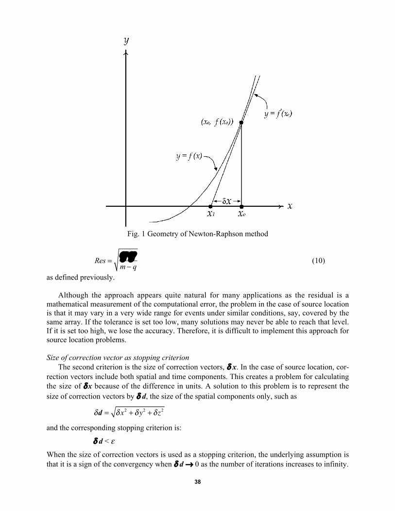
The geometry of the Newton-Raphson method is shown in Fig. 1. At each iteration stage, wedetermine the first-order derivative of the function at the trial solution. Geometrically, it repre-sents the tangent line of the function at this location. The intersection of this line with the x-axisdefines the new trial solution, xn+1. The corresponding correction vector is δx = xn − xn+1 . Fromthe figure, it is easy to verify the relation:
1
' )()(
+−=
nn
nn xx
xfxf .
The above equation is another form of the preceding equation, but with much clearer geomet-rical meaning: the slope of the tangent line represented by f'(xn) on the left-hand side of theequation is the ratio of the function value at the trial solution and the correction vector.
In summary, the Newton-Raphson method can be viewed as a procedure that we use the in-tersection of the tangent line at the x-axis to approximate the root of the function and the direc-tion of the tangent line is defined by the first order derivative of the function at the trial solution.
3.4 Stopping criteriaWhen an iterative method is used, the calculation has to be stopped at a certain point. There
are three commonly used stopping criteria for derivative methods, and their applicability for theproblem of source location is discussed next.
Residual as stopping criterionWhen residual is utilized as the stopping criterion, we stop the calculation soon after the re-
sidual is smaller than a pre-defined tolerance, such that:
Res < ε, for ε > 0,
where Res is the event residual and ε is the tolerance. The event residual is a measurement of thelocation error in terms of the total effect of the mismatch between the observed and calculatedarrival times. Mathematically, it is defined by the regression method being used. For the least-squares method, the event residual is (Ge, 1996) given by Eq. (10):
38
Fig. 1 Geometry of Newton-Raphson method
Res =
γ Tγm − q
(10)
as defined previously.
Although the approach appears quite natural for many applications as the residual is amathematical measurement of the computational error, the problem in the case of source locationis that it may vary in a very wide range for events under similar conditions, say, covered by thesame array. If the tolerance is set too low, many solutions may never be able to reach that level.If it is set too high, we lose the accuracy. Therefore, it is difficult to implement this approach forsource location problems.
Size of correction vector as stopping criterionThe second criterion is the size of correction vectors, δ x. In the case of source location, cor-
rection vectors include both spatial and time components. This creates a problem for calculatingthe size of δ x because of the difference in units. A solution to this problem is to represent thesize of correction vectors by δ d, the size of the spatial components only, such as
δd = δx2 + δy2 + δz2
and the corresponding stopping criterion is:
δ d < ε
When the size of correction vectors is used as a stopping criterion, the underlying assumption isthat it is a sign of the convergency when δ d → 0 as the number of iterations increases to infinity.
39
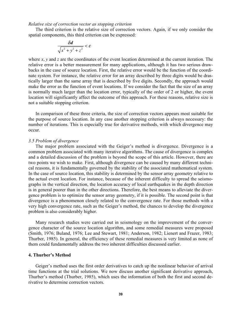
Relative size of correction vector as stopping criterionThe third criterion is the relative size of correction vectors. Again, if we only consider the
spatial components, this third criterion can be expressed:
δd
x2 + y2 + z2< ε
where x, y and z are the coordinates of the event location determined at the current iteration. Therelative error is a better measurement for many applications, although it has two serious draw-backs in the case of source location. First, the relative error would be the function of the coordi-nate system. For instance, the relative error for an array described by three digits would be dras-tically larger than the same array that is described by five digits. Secondly, the approach wouldmake the error as the function of event locations. If we consider the fact that the size of an arrayis normally much larger than the location error, typically of the order of 2 or higher, the eventlocation will significantly affect the outcome of this approach. For these reasons, relative size isnot a suitable stopping criterion.
In comparison of these three criteria, the size of correction vectors appears most suitable forthe purpose of source location. In any case another stopping criterion is always necessary: thenumber of iterations. This is especially true for derivative methods, with which divergence mayoccur.
3.5 Problem of divergenceThe major problem associated with the Geiger’s method is divergence. Divergence is a
common problem associated with many iterative algorithms. The cause of divergence is complexand a detailed discussion of the problem is beyond the scope of this article. However, there aretwo points we wish to make. First, although divergence can be caused by many different techni-cal reasons, it is fundamentally governed by the stability of the associated mathematical system.In the case of source location, this stability is determined by the sensor array geometry relative tothe actual event location. For instance, because of the inherent difficulty to spread the seismo-graphs in the vertical direction, the location accuracy of local earthquakes in the depth directionis in general poorer than in the other directions. Therefore, the best means to alleviate the diver-gence problem is to optimize the sensor array geometry, if it is possible. The second point is thatdivergence is a phenomenon closely related to the convergence rate. For those methods with avery high convergence rate, such as the Geiger’s method, the chances to develop the divergenceproblem is also considerably higher.
Many research studies were carried out in seismology on the improvement of the conver-gence character of the source location algorithm, and some remedial measures were proposed(Smith, 1976; Buland, 1976; Lee and Stewart, 1981; Anderson, 1982; Lienert and Frazer, 1983;Thurber, 1985). In general, the efficiency of these remedial measures is very limited as none ofthem could fundamentally address the two inherent difficulties discussed earlier.
4. Thurber’s Method
Geiger’s method uses the first order derivatives to catch up the nonlinear behavior of arrivaltime functions at the trial solutions. We now discuss another significant derivative approach,Thurber’s method (Thurber, 1985), which uses the information of both the first and second de-rivative to determine correction vectors.
40
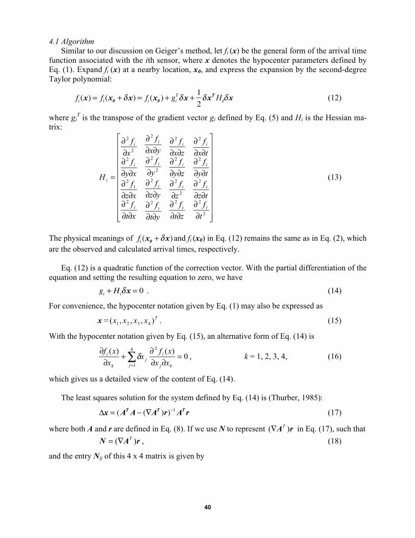
4.1 AlgorithmSimilar to our discussion on Geiger’s method, let fi (x) be the general form of the arrival time
function associated with the ith sensor, where x denotes the hypocenter parameters defined byEq. (1). Expand fi (x) at a nearby location, x0, and express the expansion by the second-degreeTaylor polynomial:
fi (x) = fi (x0 + δ x) = fi (x0 ) + gi
Tδ x +12δ xT H iδ x (12)
where giT is the transpose of the gradient vector gi defined by Eq. (5) and Hi is the Hessian ma-
trix:
⎥⎥⎥⎥⎥⎥⎥⎥⎥⎥
⎦
⎤
⎢⎢⎢⎢⎢⎢⎢⎢⎢⎢
⎣
⎡
∂∂∂∂
∂∂∂
∂∂∂
∂
∂∂∂∂∂∂∂
∂∂∂
∂
∂∂∂∂∂
∂∂∂∂∂
∂
∂∂∂∂∂
∂∂∂
∂∂∂
=
2
2
2
2
2
2
2
2
2
2
2
2
2
2
2
2
12
2
2
2
t
ftz
fty
ftx
f
zt
fz
fzy
fzx
f
yt
fyz
fy
fyx
f
xt
fxz
fxy
fx
f
H
i
i
i
i
i
i
i
i
i
i
i
i
i
i
i
i (13)
The physical meanings of fi (x0 + δ x) and fi (x0) in Eq. (12) remains the same as in Eq. (2), whichare the observed and calculated arrival times, respectively.
Eq. (12) is a quadratic function of the correction vector. With the partial differentiation of theequation and setting the resulting equation to zero, we have
gi + Hiδ x = 0 . (14)
For convenience, the hypocenter notation given by Eq. (1) may also be expressed as
x = Txxxx ),,,( 4321 . (15)
With the hypocenter notation given by Eq. (15), an alternative form of Eq. (14) is
∑=
=∂∂
∂+
∂∂ 4
1
2
0)()(
j kj
ij
k
i
xx
xfx
x
xf δ , k = 1, 2, 3, 4, (16)
which gives us a detailed view of the content of Eq. (14).
The least squares solution for the system defined by Eq. (14) is (Thurber, 1985):
Δx = (AT A − (∇AT )r)−1 AT r (17)
where both A and r are defined in Eq. (8). If we use N to represent rA )( T∇ in Eq. (17), such that
rAN )( T∇= , (18)
and the entry Nij of this 4 x 4 matrix is given by
41
k
m
k ji
kij xx
fN γ∑
= ∂∂∂
=1
2
i, j = 1, 2, 3 (19)
0=ijN i, j = 4
The step that holds the key to understand Newton’s method, and therefore Thurber’s method,is the transition from Eq. (12) to Eq. (14). Eq. (12) is a quadratic function. By the partial differ-entiation of this equation and setting the resulting equation to zero, Eq. (14) defines the extremeof this quadratic function. This extreme in Newton’s method is regarded as the optimum correc-tion vector for the trial solution, and therefore, the solution for Eq. (12).
4.2 Mechanics of iteration by first and second order derivativesFollowing the approach that the Newton-Raphson's method was used to illustrate the geomet-
ric meaning of the first order derivatives, we now use Newton’s method in one variable to dem-onstrate geometrically how the first and second order derivatives are used to determine the cor-rection vector.
Finding the root with first and second derivativesConsider the second-degree Taylor polynomial for f(x), expanded about x0,
)(")(2
1)(')()()( 0
20000 xfxxxfxxxfxf −+−+= (20)
Our goal is to determine x so that f(x) = 0. Note that f(x) in this case is expressed by a quadraticfunction of x and the best approximation of f(x) = 0 is to find the minimum of the function andthis can be done by taking the first derivative of the function with respect to x,
dx
xfxxd
dx
xfxxd
dx
xdf
dx
xdf ))(")((
2
1))(')(()()( 02
0000 −+
−+=
)(")()(' 000 xfxxxf −+=
and let the resulting equation equal to zero,
0)(")()(' 000 =−+ xfxxxf
Solving the equation for x,
)("
)('
0
00 xf
xfxx −=
the final solution can be approached iteratively by the sequence {xi} defined by
)("
)('1
i
iii xf
xfxx −=+ 0≥i (21)
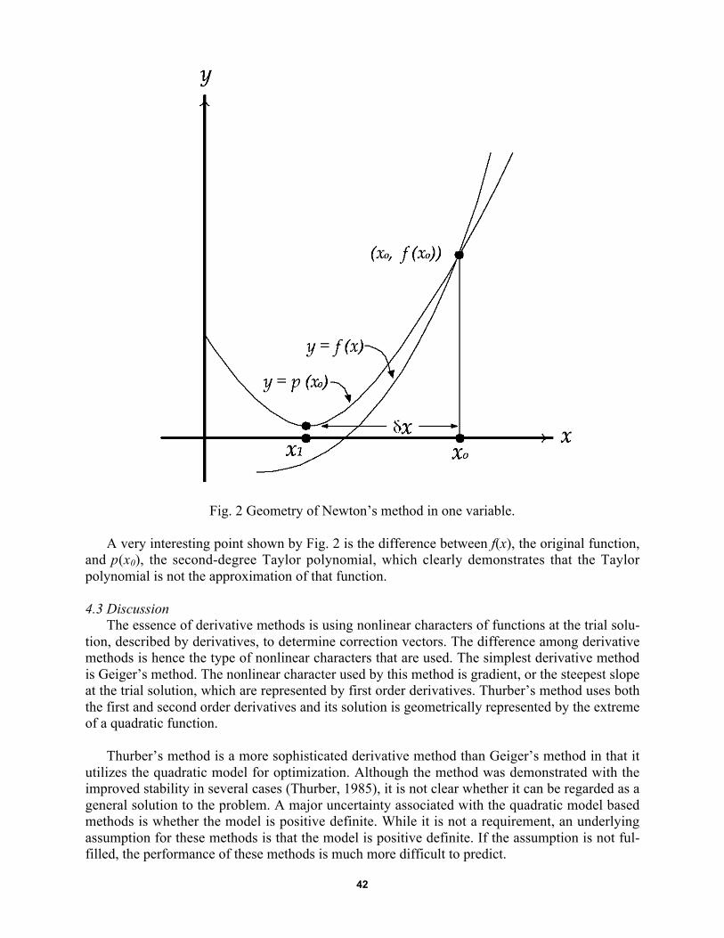
The geometry of this solution process is illustrated in Fig. 2. The second-degree Taylor poly-nomial, denoted by p(x0) in the figure, is used to represent the function at the neighborhood of x0.The extreme of this polynomial, x1, is considered by Newton’s method as the optimum solutionwhich becomes the new trial solution. Eq. (21) is a mathematical definition of this extreme.
42
Fig. 2 Geometry of Newton’s method in one variable.
A very interesting point shown by Fig. 2 is the difference between f(x), the original function,and p(x0), the second-degree Taylor polynomial, which clearly demonstrates that the Taylorpolynomial is not the approximation of that function.
4.3 DiscussionThe essence of derivative methods is using nonlinear characters of functions at the trial solu-
tion, described by derivatives, to determine correction vectors. The difference among derivativemethods is hence the type of nonlinear characters that are used. The simplest derivative methodis Geiger’s method. The nonlinear character used by this method is gradient, or the steepest slopeat the trial solution, which are represented by first order derivatives. Thurber’s method uses boththe first and second order derivatives and its solution is geometrically represented by the extremeof a quadratic function.
Thurber’s method is a more sophisticated derivative method than Geiger’s method in that itutilizes the quadratic model for optimization. Although the method was demonstrated with theimproved stability in several cases (Thurber, 1985), it is not clear whether it can be regarded as ageneral solution to the problem. A major uncertainty associated with the quadratic model basedmethods is whether the model is positive definite. While it is not a requirement, an underlyingassumption for these methods is that the model is positive definite. If the assumption is not ful-filled, the performance of these methods is much more difficult to predict.
43
5. Simplex Method
The Simplex method is a relatively new method developed by Nelder and Mead (1965). Itsearches the minimums of mathematical functions through function comparison. The methodwas introduced for the source location purpose in late 1980s by Prugger and Gendzwill (Pruggerand Gendzwill, 1988; Gendzwill and Prugger, 1989). The mathematical procedures and relatedconcepts in error estimation for this method were further discussed by Ge (1995). Readers shouldbe aware that the Simplex method discussed here is different from the one used in linear pro-gramming where it refers an algorithm for a special type of linear problems.
5.1 Method conceptThe Simplex method starts from the idea that, for a given set of arrival times associated with
a set of sensors, an error can be calculated for any point by comparing the observed and the cal-culated arrival times. An error space is thus the one in which every point is defined by an asso-ciated error, and the point with the minimal error is the event location.
The process of searching for the minimal point with the Simplex method is unique. The so-lution is said to be found when a Simplex figure falls into the depression of the error space. TheSimplex is a geometric figure which contains one more vertex than the dimension of the space inwhich it is used. A simplex for a two dimensional space is a triangle, a simplex for a three di-mensional space is a tetrahedron, etc.
The search for the final solution with the Simplex source location method involves four gen-eral steps:
i) setting an initial Simplex figure;ii) calculating errors for vertices;iii) moving Simplex figures; andiv) examining the status of convergency.
At the beginning of search, an initial Simplex figure has to be set, which is then rollingthrough the error space, expanding, contracting, shrinking and turning towards the minimal errorpoint of the space. The movement of the Simplex figure is governed by the error distribution atits vertex, which is calculated each time when the Simplex figure is reshaped.
5.2 Simplex figure and its initial settingIt is understood from the earlier discussion that the Simplex is a geometric figure that con-
tains one more vertex than the dimension of the space in which it is used. Because a source loca-tion problem is spanned by not only its geometric dimensions, but also time dimension, the Sim-plex figure will be tetrahedron and five-vertices for two and three geometrical problems, respec-tively, if we apply the Simplex method directly to our source location problems.
A more convenient approach is to consider spatial coordinates and origin time “separately” inthat error spaces are already optimized in terms of origin time. With this treatment, the dimen-sion of the Simplex figures is solely determined by the geometric dimension of the source loca-tion problems: a triangle for two-dimensional problems and a tetrahedron for three-dimensionalproblems. We will discuss the mathematical procedure of this approach in the next section.
There is no rigid guideline regarding how to set the initial Simplex figure. For the purpose ofefficiency, one may want to set it near the potential location with a reasonable size. Care must
44
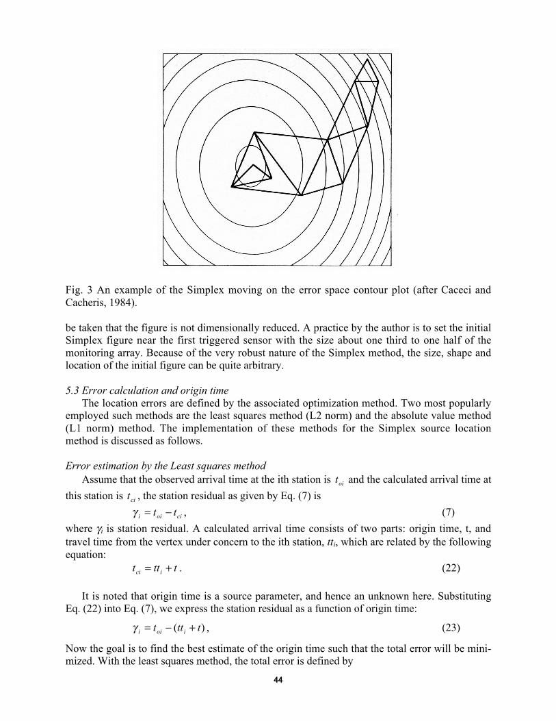
Fig. 3 An example of the Simplex moving on the error space contour plot (after Caceci andCacheris, 1984).
be taken that the figure is not dimensionally reduced. A practice by the author is to set the initialSimplex figure near the first triggered sensor with the size about one third to one half of themonitoring array. Because of the very robust nature of the Simplex method, the size, shape andlocation of the initial figure can be quite arbitrary.
5.3 Error calculation and origin timeThe location errors are defined by the associated optimization method. Two most popularly
employed such methods are the least squares method (L2 norm) and the absolute value method(L1 norm) method. The implementation of these methods for the Simplex source locationmethod is discussed as follows.
Error estimation by the Least squares methodAssume that the observed arrival time at the ith station is oit and the calculated arrival time at
this station is cit , the station residual as given by Eq. (7) is
cioii tt −=γ , (7)
where γi is station residual. A calculated arrival time consists of two parts: origin time, t, andtravel time from the vertex under concern to the ith station, tti, which are related by the followingequation:
tttt ici += . (22)
It is noted that origin time is a source parameter, and hence an unknown here. SubstitutingEq. (22) into Eq. (7), we express the station residual as a function of origin time:
)( tttt ioii +−=γ , (23)
Now the goal is to find the best estimate of the origin time such that the total error will be mini-mized. With the least squares method, the total error is defined by
45
∑ 2iγ
and it is minimized when the origin time is determined by the equation
0)( 2
=∑dt
d iγ
Solving the above equation, the best estimate of the origin time is
n
tt
n
tt ii ∑∑ −= (24)
By substituting Eq. (24) into Eq. (23), we express the station residual in terms of observed arrivaltime and calculated travel time:
)()(n
tttt
n
tt i
ii
ii∑∑ −−−=γ (25)
The event residual is
qmRes
−= ∑ 2
iγ . (26)
Eq. (26) is the equation that is used for the error calculation for each vertex if the least squaresmethod is used. Note that the origin time with this approach is given by Eq. (24).
Error estimation by the absolute value methodFor the absolute value method, the total error is defined by
∑ iγ .
The best estimate of the origin time has to satisfy the objective function
Minimize (∑ iγ ).
Substituting Eq. (23) into the above expression, we have
Minimize (∑ +− )( tttt ii ).
For a set of linear equations with the form of
,ibx =
where x is the variable to be estimated and bi is a constant, the analytical solution of the best fitfor x defined by the L1 misfit norm is the median of bis (Chavatal, 1983). Accordingly, the bestfit of the origin time is the median of all (ti – tti). Let us denote it as tm. The station residual de-fined by the absolute value method is therefore
miii tttt −−=γ (27)
and the total error is
∑∑ −−= miii ttttγ . (28)
Eq. (28) is the equation that is used for the error calculation for each vertex if the absolute valuemethod is used. Note that the origin time with this approach is the median of all (ti – tti).
46
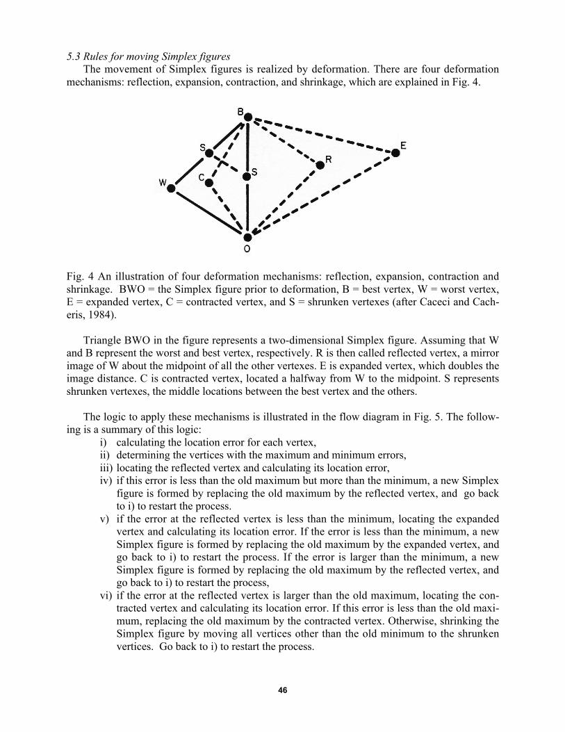
5.3 Rules for moving Simplex figuresThe movement of Simplex figures is realized by deformation. There are four deformation
mechanisms: reflection, expansion, contraction, and shrinkage, which are explained in Fig. 4.
Fig. 4 An illustration of four deformation mechanisms: reflection, expansion, contraction andshrinkage. BWO = the Simplex figure prior to deformation, B = best vertex, W = worst vertex,E = expanded vertex, C = contracted vertex, and S = shrunken vertexes (after Caceci and Cach-eris, 1984).
Triangle BWO in the figure represents a two-dimensional Simplex figure. Assuming that Wand B represent the worst and best vertex, respectively. R is then called reflected vertex, a mirrorimage of W about the midpoint of all the other vertexes. E is expanded vertex, which doubles theimage distance. C is contracted vertex, located a halfway from W to the midpoint. S representsshrunken vertexes, the middle locations between the best vertex and the others.
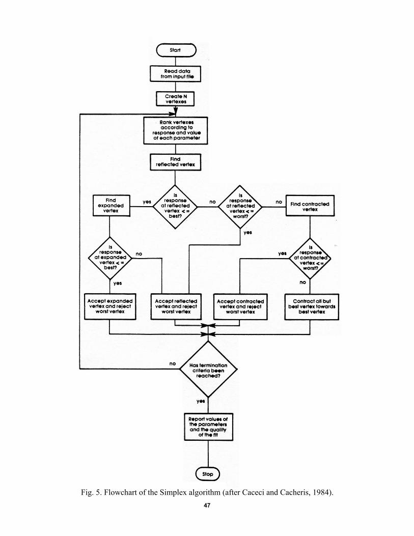
The logic to apply these mechanisms is illustrated in the flow diagram in Fig. 5. The follow-ing is a summary of this logic:
i) calculating the location error for each vertex,ii) determining the vertices with the maximum and minimum errors,iii) locating the reflected vertex and calculating its location error,iv) if this error is less than the old maximum but more than the minimum, a new Simplex
figure is formed by replacing the old maximum by the reflected vertex, and go backto i) to restart the process.
v) if the error at the reflected vertex is less than the minimum, locating the expandedvertex and calculating its location error. If the error is less than the minimum, a newSimplex figure is formed by replacing the old maximum by the expanded vertex, andgo back to i) to restart the process. If the error is larger than the minimum, a newSimplex figure is formed by replacing the old maximum by the reflected vertex, andgo back to i) to restart the process,
vi) if the error at the reflected vertex is larger than the old maximum, locating the con-tracted vertex and calculating its location error. If this error is less than the old maxi-mum, replacing the old maximum by the contracted vertex. Otherwise, shrinking theSimplex figure by moving all vertices other than the old minimum to the shrunkenvertices. Go back to i) to restart the process.
47
Fig. 5. Flowchart of the Simplex algorithm (after Caceci and Cacheris, 1984).
48
5.5 Examining the status of convergencyIn section 3.4 we discussed the stopping criterion for derivative methods and determined that
the size of correction vectors would be most appropriate for the purpose of source location. It isfor the same reason that we use the size of Simplex figures as the measurement of the conver-gency status of Simplex solutions. We accept the solution if the size of the Simplex figure is lessthan the tolerance. The size may be defined differently. For instance, the average distance from avertex to others would be a convenient and representative measurement of the size.
5.6 DiscussionThe Simplex method offers several distinctive advantages over derivative methods. The most
important one is that divergence is impossible. The author manually examined several thousandsof location data by the Simplex method and did not observe a single divergence case. In fact, thesame Simplex code developed by the author has been installed at a numerous mine sites for thecontinuous monitoring for many years and there has been no divergence problems ever reported.The reason for this robust performance is that the Simplex figure will not leave the lowest errorpoint which has been found unless a better one is located. Therefore, the Simplex method willalways keep the best solution that has been found, whereas for others it may be lost in iterationprocesses. This character is especially important for the automated monitoring.
The other important advantage of the method is its flexibility. Unlike derivative methods,with which arrival time functions have to be established prior to the analysis, arrival time func-tions used in the Simplex method can be established during the data processing, which is a nec-essary condition in order to handle many sophisticated problems.
A frequently mentioned advantage of the Simplex method is that we avoid many computa-tional problems associated with partial derivatives and matrix inversions. It is, however, impor-tant to understand that this is not equivalent to say that the underlying problems are also gone.For instance, an ill-conditioned matrix in source location is a reflection of the instability of theassociated mathematical system. It would be a serious mistake to expect the disappearance of theproblem by using the Simplex method. The truth is that the problem is physical; its existence isindependent of the solution methods.
6. Conclusions
Iterative methods are of primary importance in source location methods. This is because oftheir flexibility in dealing with arrival time functions, which is essential for realistically ap-proaching a great majority of source location problems. Non-derivative methods have to assumea single velocity for all channels, which severely limits their application.
The best known group of iterative methods is derivative algorithms. With derivative meth-ods, we approach the final solution through a continuous updating process of trial solution, andthis is done by adding the correction vector found from the previous iteration at each stage. Thecorrection vector is determined by the assessment of nonlinear behavior of arrival time functionsat the trial solution. The difference among derivative methods is therefore the type of the nonlin-ear behavior that is utilized.
The nonlinear behavior used by Geiger’s method is the gradient of arrival time functions, orthe steepest direction of these functions, represented by the first-order derivatives. The one util
49
ized by Thurber’s method is the extreme of the quadratic functions, which is the second-degreeof Taylor polynomials, including both the first- and second-order derivatives..
Because the nonlinear behaviors are used decisively for the calculation of correction vectors,derivative methods, such as Geiger’s method and Thurber’s method, are inherently efficient, andoffer superior performance to other iterative methods. The final solutions are usually approachedwithin a few iterations if the associated systems are stable.
A shortcoming of derivative methods is divergence. While the cause of divergence is com-plex and a detailed discussion of the problem is beyond the scope of this article, it is important toknow that divergence, in general, reflects the problem of instability, which, in turn, is largelygoverned by the sensor array geometry.
The Simplex method is the most important source location method emerged in recent years.Because of its unique iteration approach, divergence is impossible. This has given the method ahuge advantage over derivative methods. The other major advantage of the method is its flexi-bility to deal with complicated velocity models. Unlike derivative methods, with which arrivaltime functions have to be established prior to the analysis, arrival time functions used in theSimplex method can be established during the data processing, which is a necessary condition inorder to handle many sophisticated problems.
Finally, we would like to emphasize that source location is a subject affected by many factorsand the location algorithm is only one of them. In order to use a location algorithm efficiently,we need not only a good understanding of the algorithm itself, but also a perspective view onhow the algorithm relates to other factors. The two most important factors are sensor array ge-ometry and errors associated with input data.
Sensor array geometry and system stabilityThe importance of the sensor array geometry in AE source location lies on the fact that we
would never be able to eliminate input errors completely and the impact of these initial errors onthe final location accuracy is controlled by the sensor array geometry (Ge, 1988). Good arraygeometry can effectively limit the impact of initial errors while a poor one will maximize the im-pact. In other words, the stability of the associated mathematical system is determined by thesensor array geometry. Therefore, the sensor array geometry is fundamental for an accurate andreliable AE source location.
Understanding the relation between sensor array geometry and system stability is importantfrom two perspectives. First, the stability of an event location is independent of the location algo-rithm being used; that is, we can not change the degree of the sensitivity of a solution to initialerrors by switching the location algorithm. If we want to improve the reliability of event loca-tions, the only means is to improve the sensor array geometry. There is no other way around.
Second, a phenomenon that is closely associated with an unstable system is divergence. It ismore difficult to approach the solution numerically when the associated system is unstable. It is,however, important to note that the convergence character does differ from method to method.We can reduce the risk of divergence by choosing an algorithm with the better convergencecharacter, and Simplex method is such an example.
50
Errors associated with input dataThere are a number of error sources for AE source location data. The obvious ones are tim-
ing, velocity model and sensor coordinates. The one that is often not recognized but may causemost damages is misidentification of arrival types.
An assumption that is frequently made in AE source location is P-wave triggering. In reality,many arrivals are due to S-waves or even not related signals called outlier. An outlier may becaused by either culture noises or the interference of other events. The analysis of AE datashows that S-wave arrivals may account for as much as more than 50% of total arrivals (Ge andKaiser, 1990). As S-wave velocity is typically half of the P-wave velocity, mixing of P- and S-wave arrivals immediately introduces a large and systematical error to the location system. Thishas been the primary reason responsible for the poor AE source location accuracy in the past.
Although there are means to reduce the impact of input errors, such as optimization of thesensor array geometry and statistical analysis, one should not expect that any of these methodswould be able to deal with large and systematical errors. These errors have to be detected andeliminated before the location process starts.
Acknowledgments
I am grateful to Dr. Kanji Ono for his encouragement to write my research experience in thearea, and his detailed review of the manuscript and comments. I thank Dr. Hardy for his thor-ough review and the anonymous reviewer for his comments and suggestions to improve themanuscript.
References
Anderson, K. R., (1982). Robust earthquake location using M-estimates, Phys. Earth andPlanet Int., 30, 119-130.
Billings, S. D., B. L. N. Kennett, and M. S. Sambridge, (1994). Hypocentre location: geneticalgorithms incorporating pro lem-specific information, Geophys. J. Int. 118, 693-700.
Buland, R., (1976). The mechanics of locating earthquakes, Bull. Seism. Soc. Am. 66, 173-187.
Burden, R. L., J. D. Faires and A. C. Beynolds (1981). Numerical analysis, Prindle, Weber &Schmidt, Boston, Massachusetts.
Caceci, M. S. and W. P. Cacheris (1984). Fitting curves to data (the Simplex algorithms isthe answer), Byte 9, 340-362.
Ge, M., (1988). Optimization of Transducer array geometry for acousticemission/microseismic source location. Ph.D. Thesis, The Pennsylvania State University,Department of Mineral Engineering, 237 p.
Ge, M. and P. K. Kaiser (1990). Interpretation of physical status of arrival picks formicroseismic source location. Bull. Seism. Soc. Am. 80, pp. 1643-1660.
51
Ge, M. (1995). Comment on "Microearthquake location: a non-linear approach that makesuse of a Simplex stepping procedure" by A. Prugger and D. Gendzwell, Bull. Seism. Soc. Am.85, 375-377.Geiger, L. (1910). Herbsetimmung bei Erdbeben aus den Ankunfzeiten, K.Gessell. Will. Goett. 4, 331-349.
Geiger, L. (1912). Probability method for the determination of earthquake epicentres fromthe arrival time only, Bull. St. Louis. Univ. 8, 60-71.
Gendzwill, D. and A. Prugger (1989). Algorithms for micro-earthquake location, in Proc. 4th
Conf. Acoustic emission/Microseismic Activity in Geologic Structures, Trans Tech.Publications, Clausthal-Zellerfeld, Germany, 601-605.
Holland, J. H. (1975). Adaption in Natural and Artificial Systems, The University ofMichigan Press, Ann Arbor.
Kennett, B. L. N. and M. S. Sambridge, (1992). Earthquake location – genetic algorithms forteleseisms, Phys. Earth and Planet Int., 75, 103 -110.
Lee, W. H. K. and S. W. Stewart (1981). Principles and applications of microearthquakenetworks, Adv. Geophys. Suppl. 2.
Lienert, B. R. and L. N. Frazer (1983). An improved earthquake location algorithm, EOS,Trans. Am. Geophys. Union, 64, 267.
Nelder, J. A. and R. Mead (1965). A simplex method for function minimization, Computer J.7, 308-313.
Prugger, A. and D. Gendzwill (1989). Microearthquake location: a non-linear approach thatmakes use of a Simplex stepping procedure, Bull. Seism. Soc. Am. 78, 799-815.
Sambridge, M., K. Gallagher, (1993). Earthquake hypocenter location using geneticalgorithms, Bull. Seism. Soc. Am. 83, 1467-1491.
Smith, E. G. C., (1976). Scaling the equations of condition to improve conditioning, Bull.Seism. Soc. Am. 66, 2075-2076.
Strang, G. (1980). Linear algerbra and its applications, Academic Press Inc., New York, NewYork.
Thurber, C. H. (1985). Nonlinear earthquake location: theory and examples, Bull. Seism. Soc.Am. 75, 779-790.
Xie, Z, T. W. Spencer, P. D. Rabinowitz, and D. A. Fahlquist, (1996). A new regionalhypocenter location method, Bull. Seism. Soc. Am. 86, 946-958.