Analysis of Temperature and Humidity Effects on Horizontal ...

Air Force Institute of TechnologyAFIT Scholar

Theses and Dissertations Student Graduate Works

3-23-2018

Analysis of Temperature and Humidity Effects onHorizontal Photovoltaic PanelsCorey J. Booker

Follow this and additional works at: https://scholar.afit.edu/etd

Part of the Numerical Analysis and Computation Commons, and the Power and EnergyCommons

This Thesis is brought to you for free and open access by the Student Graduate Works at AFIT Scholar. It has been accepted for inclusion in Theses andDissertations by an authorized administrator of AFIT Scholar. For more information, please contact [email protected].

Recommended CitationBooker, Corey J., "Analysis of Temperature and Humidity Effects on Horizontal Photovoltaic Panels" (2018). Theses and Dissertations.1876.https://scholar.afit.edu/etd/1876

https://scholar.afit.edu?utm_source=scholar.afit.edu%2Fetd%2F1876&utm_medium=PDF&utm_campaign=PDFCoverPages

https://scholar.afit.edu/etd?utm_source=scholar.afit.edu%2Fetd%2F1876&utm_medium=PDF&utm_campaign=PDFCoverPages

https://scholar.afit.edu/graduate_works?utm_source=scholar.afit.edu%2Fetd%2F1876&utm_medium=PDF&utm_campaign=PDFCoverPages

https://scholar.afit.edu/etd?utm_source=scholar.afit.edu%2Fetd%2F1876&utm_medium=PDF&utm_campaign=PDFCoverPages

http://network.bepress.com/hgg/discipline/119?utm_source=scholar.afit.edu%2Fetd%2F1876&utm_medium=PDF&utm_campaign=PDFCoverPages



https://scholar.afit.edu/etd/1876?utm_source=scholar.afit.edu%2Fetd%2F1876&utm_medium=PDF&utm_campaign=PDFCoverPages

mailto:[email protected]

AFIT-ENV-MS-18-M-180

ANALYSIS OF TEMPERATURE AND HUMIDITY EFFECTS ON

HORIZONTAL PHOTOVOLTAIC PANELS

THESIS

Corey J. Booker, Capt, USAF


DEPARTMENT OF THE AIR FORCE AIR UNIVERSITY

AIR FORCE INSTITUTE OF TECHNOLOGY

Wright-Patterson Air Force Base, Ohio

DISTRIBUTION STATEMENT A. APPROVED FOR PUBLIC RELEASE;

DISTRIBUTION UNLIMITED

The views expressed in this thesis are those of the author and do not reflect the official

policy or position of the United States Air Force, Department of Defense, or the United

States Government. This material is declared a work of the United States Government

and is not subject to copyright protection in the United States.




THESIS

Presented to the Faculty

Department of Engineering Management

Graduate School of Engineering and Management

Air Force Institute of Technology

Air University

Air Education and Training Command

In Partial Fulfillment of the Requirements for the

Degree of Master of Science in Engineering Management

Corey J. Booker

Captain, USAF

23 Feb 2018

DISTRIBUTION STATEMENT A. APPROVED FOR PUBLIC RELEASE;

DISTRIBUTION UNLIMITED


ANALYSIS OF TEMPERATURE AND HUMIDITY EFFECTS ON HORIZONTAL

PHOTOVOLTAIC PANELS

Corey J. Booker

Captain, USAF

Committee Membership:

Alfred E. Thal, Jr., PhD Chair

Diedrich Prigge V, PhD Member

Brent T. Langhals, PhDMember

Lt Col Torrey J. Wagner, PhD

Member

iv

Abstract

The United States Air Force seeks to address power grid vulnerability and bolster

energy resilience through the use of renewable energy sources. Air Force Institute of

Technology engineers designed and manufactured control systems to monitor power

production from the most widely-used silicon-based solar cells at 38 testing locations

around the globe spanning the majority of climate types. Researchers conducted

multivariate regression analysis to establish a statistical relationship between photovoltaic

power output, ambient temperature, and humidity pertaining to monocrystalline and

polycrystalline photovoltaic panels. Formulated models first characterized power output

globally, then by specific climate type with general inaccuracy. Location-specific models

are provided with varying accuracy, allowing a number of locations to predict energy

output and make decisions regarding future energy projects. It was found that additional

predictor variables are required to hone model accuracy. Recommendations are made

that modify the current study for the purpose of increasing data quality as well as

ensuring the validity and accuracy of resulting regression models and the future ability to

forecast power production for use by decision-making authorities. Further, a full year of

measurements combined with proposed modifications will demonstrate feasibility of

utilizing horizontal photovoltaic technology.

v

Table of Contents

Page

Abstract .............................................................................................................................. iv

Table of Contents .................................................................................................................v

List of Figures ................................................................................................................... vii

List of Tables ..................................................................................................................... ix

I. INTRODUCTION ...........................................................................................................1

General Issue and Background........................................................................................1 Problem Statement ..........................................................................................................4 Research Objectives ........................................................................................................5 Investigative Questions ...................................................................................................6

Methodology Overview ..................................................................................................6 Assumptions and Limitations ..........................................................................................7

Organization of Thesis ....................................................................................................8

II. LITERATURE REVIEW ...............................................................................................9

Energy Security ...............................................................................................................9 Vulnerability of U.S. Grid ....................................................................................... 11

DoD Considerations ................................................................................................ 12 Photovoltaic Basics .......................................................................................................13

Operating Principles ............................................................................................... 14

Panel Type ............................................................................................................... 17 Panel Orientation .................................................................................................... 19

Photovoltaic Pavement Systems ...................................................................................20 Global Position and Climate Types ..............................................................................24 Temperature and Humidity Performance Models .........................................................27

III. METHODOLOGY .....................................................................................................31

Test System Design, Manufacture, and Distribution ....................................................31 Methods of Analysis .....................................................................................................37

Multivariate Linear Regression .............................................................................. 38 Variance Testing ..................................................................................................... 40

Potential Sources of Error .............................................................................................41

IV. ANALYSIS AND RESULTS.....................................................................................42

Data Quality ..................................................................................................................42

vi

Performance Modeling ..................................................................................................44 Key Assumptions ..................................................................................................... 46 Monocrystalline Models .......................................................................................... 47 Polycrystalline Models ............................................................................................ 53 Regression Models by Location .............................................................................. 55

Model Coefficients ................................................................................................... 61 Surface Variance Test ............................................................................................. 62

V. CONCLUSIONS AND RECOMMENDATIONS ......................................................64

Key Points .....................................................................................................................64 Recommendations for Future Research ........................................................................65

Appendix – Performance Model Analyses ........................................................................68

References ..........................................................................................................................77

vii

List of Figures

Page

Figure 1. Energy Consumption within the DoD ................................................................ 2

Figure 2. Energy Council Governance Structure ............................................................. 10

Figure 3. A chunk of semi-conducting silicon metal ....................................................... 13

Figure 4. Simplified depiction of crystalline silicon ........................................................ 14

Figure 5. n and p type silicon combined to create a P-N junction ................................... 15

Figure 6. Post-photon strike on PV cell, electron freed ................................................... 16

Figure 7. freed electron flow ............................................................................................ 16

Figure 8. Electron flow, n-type SI, through load, back to p-type SI ................................ 16

Figure 9. Various PV types .............................................................................................. 18

Figure 10. SRI's product - photovoltaic pavement system .............................................. 21

Figure 11. Test site at Missouri DOT .............................................................................. 22

Figure 12. First public test in Sandpoint, Idaho ............................................................... 23

Figure 13. Köppen climate types ..................................................................................... 25

Figure 14. Control unit housing ....................................................................................... 32

Figure 15. Power-monitoring circuit................................................................................ 33

Figure 16. Raspberry Pi ................................................................................................... 34

Figure 17. Raspberry Pi Components .............................................................................. 34

Figure 18. RockBlock MK2 ............................................................................................. 35

Figure 19. System health update ...................................................................................... 35

Figure 20. 12V 12Ah battery with DC controller ............................................................ 36

viii

Figure 21. 12V battery DC control unit ........................................................................... 37

Figure 22. Complete test system with battery and charging panel .................................. 37

Figure 23. Linear regression output example .................................................................. 38

Figure 24. Example two-sample t-test results using JMP software ................................. 41

Figure 25. Monocrystalline correlations at select locations ............................................. 46

Figure 26. Polycrystalline correlations at select locations ............................................... 47

Figure 27. Monocrystalline global model ........................................................................ 49

Figure 28. Post-transformation residual plots with predictors indicating linearity ......... 49

Figure 29. Cone-shaped residual pattern indicating non-linearity ................................... 50

Figure 30. two-sample t-test comparing ground and roof system output ........................ 63

Figure 31. temperature and humidity distributions by surface type ................................ 63

Figure 32. GMX101 Solar Radiation Sensor ................................................................... 66

Figure 33. Monocrystalline model and diagnostics for boreal climate ............................ 68

Figure 34. Monocrystalline model and diagnostics for dry climate ................................ 69

Figure 35. Monocrystalline model and diagnostics for temperate climate ...................... 70

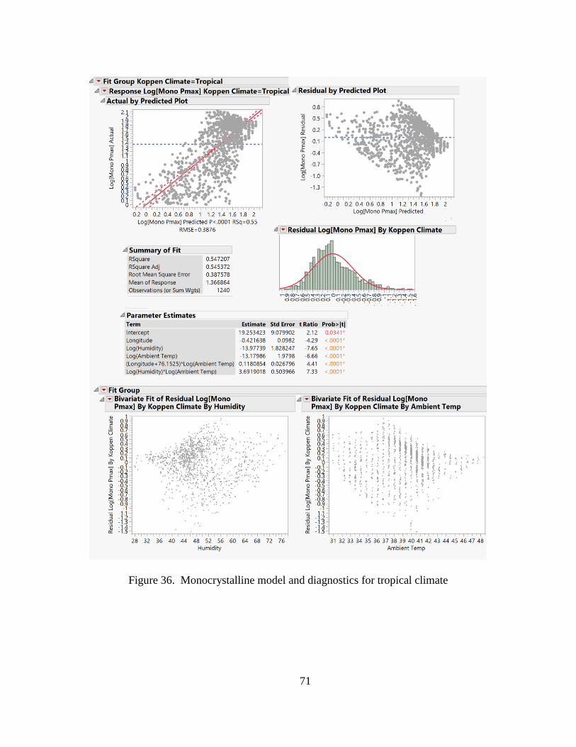
Figure 36. Monocrystalline model and diagnostics for tropical climate ......................... 71

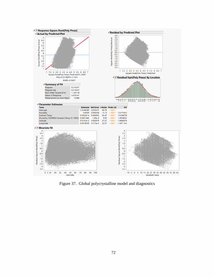
Figure 37. Global polycrystalline model and diagnostics ................................................ 72

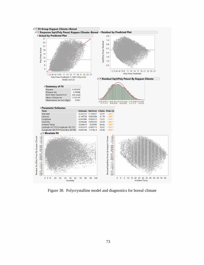
Figure 38. Polycrystalline model and diagnostics for boreal climate .............................. 73

Figure 39. Polycrystalline model and diagnostics for dry climate................................... 74

Figure 40. Polycrystalline model and diagnostics for temperate climate ........................ 75

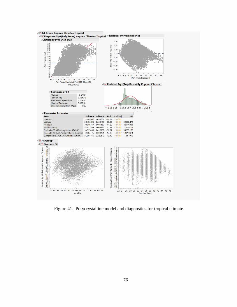
Figure 41. Polycrystalline model and diagnostics for tropical climate ............................ 76

ix

List of Tables

Page

Table 1. One year of test data in Oracle, AZ ................................................................... 23

Table 2. Climate types and locations analyzed ............................................................... 26

Table 3. Competing Temperature/Efficiency Equations ................................................. 28

Table 4. Competing Temperature/Power Equations ........................................................ 29

Table 5. Test Site participation ........................................................................................ 43

Table 6. Analyzed test locations and their corresponding Kӧppen climate types ........... 43

Table 7. Transformations of Y to improve model performance ...................................... 45

Table 8. Monocrystalline regression models and predictor effects by location .............. 57

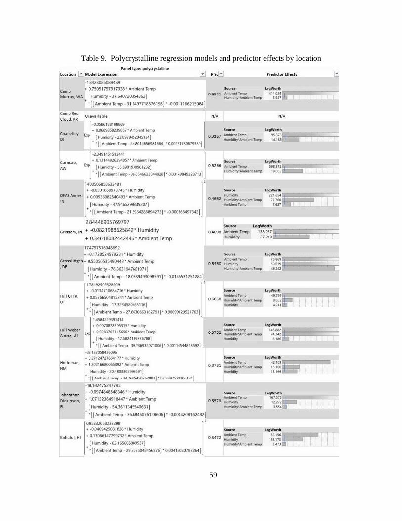
Table 9. Polycrystalline regression models and predictor effects by location ................. 59

1



I. INTRODUCTION

Energy resilience is a global issue and an especially key concern for the United

States Air Force. Meeting energy needs through practical and regulatory requirements

will necessitate exploration of renewable technologies. One such technology is

photovoltaic (PV) panels, commonly referred to as solar panels, which convert solar

irradiance into usable electricity. This research builds upon a prior feasibility study on

the use of PV pavement technology and will test its underlying principle: horizontal

placement of silicon-based PV panels to capture direct and diffuse radiation. To

accomplish this, power output must be measured in various climate types around the

world having broad temperature and humidity ranges for a sufficient period of time. This

will allow researchers to observe and record relationships between environmental factors

affecting panel performance.

General Issue and Background

Securing energy resources for the purpose of national security is a primary focus

for United States military and political leadership. The National Defense Authorization

Act of 2010 allocated resources for use by the United States Department of Defense

(DoD) and mandated that 25% of energy usage by the department be derived from

renewable sources by the end of 2025 (U.S. Congress, 2010). One such renewable source

is solar energy. This energy source can be captured by PV technology, allowing

2

absorption of solar radiation to produce electricity via commercially available silicon-

based panels. The U.S. Air Force, bearing the majority of the burden imposed by

congressional mandate as shown in Figure 1, has made significant investments toward

arrays of PV panels at installations such as Nellis Air Force Base (AFB) and Davis-

Monthan AFB, utilizing large amounts of real estate readily available at these locations

(PEW Project, 2014; U.S. Air Force, 2014).

Figure 1. Energy Consumption within the DoD (AFCEC, 2014)

Since military installations may be limited in their available land to an extent that

prohibits enterprise-wide adoption of large PV arrays, alternative solutions must be

sought. One example is rooftop PV, which requires extensive and costly structural

modifications to allow for installation. Because of these challenges, a different method

of utilizing PV will be necessary lest the technology be abandoned in favor of renewable

energy sources with a higher perceived feasibility.

Great potential exists for the Air Force to continue building energy resilience and

complying with congressional mandate. An emerging technology, photovoltaic

pavement systems, provided the impetus for this research due to their flat orientation.

3

Horizontal positioning of PV panels are not normally considered due to decreased

efficiency in capturing direct solar radiation. However, there is data that suggests

horizontal PV may be more efficient at capturing diffuse solar radiation and may be

significantly influenced by temperature and humidity (Brusaw & Brusaw, 2016). In

addition, there is a multitude of performance models characterizing power output as a

function of temperature and humidity (Sukamongkol et al., 2001; Rosell & Ibanez, 2006;

Skoplaki & Palyvos, 2008; Koussa et al., 2012). It is important to note that these models

were obtained using tilted panels aimed at maximizing direct radiation exposure.

Therefore, insights from current literature apply to applications using tilted panels and

not necessarily to those using horizontal panels.

For applications utilizing a horizontal tilt, the goal is assessment of PV

performance at different locations around the world comprising a variety of climate

types, temperatures, and humidity ranges. There may be many environmental factors to

consider in assessing PV performance through multiple successive research efforts. This

research narrows its focus to determining performance impacts of temperature and

humidity on two types of PV panels: mono-crystalline and poly-crystalline. Currently, 24

and 27 performance models exist for efficiency and power, respectively, with

temperature as an independent variable. In addition, the Köppen-Geiger Climate

Classification methodology was utilized in a prior study to produce several climate

categories in which Air Force installations are located (Nussbaum, 2017). These

categories result in a great amount of variance in the effects of ambient temperature and

humidity in mono- and polycrystalline PV panels. The study also identified 25 global

4

regions in which test systems would need to be placed. Further details on this process,

including test site selection, are provided in the following chapter. This effort

implements the proposed global test to analyze data gathered from 37 installations in

which the Air Force operates. Simultaneous research examines categorical data from this

test and performs logistical regression to determine which military installations and their

corresponding climate types are ideally suited for horizontal PV panels in any given

application. Follow-on studies will build upon the knowledge garnered through this line

of research to gain a more complete understanding of the benefits and risks of full

investment into this technology.

Problem Statement

As stated in the previous section, there are many performance models

characterizing power output as a function of temperature and a considerable number of

separate models accounting for humidity. Again, these accounted for non-horizontal PV

panels and users of PV technology may be constrained to horizontal positioning of

panels. Thus, users would remain unable to predict the amount of electricity produced at

any given time due to a lack of data in their respective climates and global positions. A

deeper understanding is needed regarding performance at various locations with a broad

range of temperature and humidity. This would serve to arm leadership with decision-

making power in considering PV-related projects on military installations or within any

interested organization.

5

Research Objectives

To fully analyze and predict power output as a function of temperature and

humidity, data must be gathered from as many of the 25 stated global regions as possible

to account for any variation due to different climate types. In addition, a dataset spanning

a full year is necessary to account for seasonal changes that are likely to have significant

impact on panel performance. A larger sample size covering the entire year will hone the

resulting regression model’s accuracy, with limitations. Data spanning a greater number

of years would be required to obtain the most accurate model possible. An analysis of

the data allows for comparison with existing performance models to ascertain which most

accurately predicts power output over the course of a year. Quality of data that lacks

significant gaps or errors is important to establish confidence in the accuracy of new

regression models based on ambient temperature and humidity. After constructing a new

regression model, a tolerable range of values pertaining to ambient conditions that

maximize power output can be discovered.

The aim of this study will be to build upon previous research and implement the

proposed study by Nussbaum. The end goal in assessing the feasibility of horizontal PV

technology remains. To build toward that end, this study aims to refine the accuracy of

existing ambient temperature/humidity dependent performance models that characterize

horizontal silicon-based PV panels in a variety of previously identified test regions.

Current data gathered by Brusaw and Brusaw only encapsulates latitudes within the U.S.,

though the Air Force maintains operations at continental U.S. (CONUS) and overseas

(OCONUS) installations. Collecting data and identifying performance coefficients at

6

military installations operating on other continents will provide a more robust

performance characterization.

Investigative Questions

Test systems monitoring power output at each test site measured and recorded

power readings for an initial period of one year. Time constraints prompted preliminary

analysis of data spanning a shorter timeframe, discussed in chapters III and IV.

Following data compilation for initial analysis, research utilized multivariate regression

techniques to answer the following primary research questions:

1. Which existing model most accurately predicts PV performance with respect

to ambient temperature and humidity?

2. How accurate is an empirically established regression model based on ambient

temperature, ambient humidity, and global position for mono- and poly-

crystalline silicon PV panels?

3. Which ambient conditions are optimal for use of horizontally inclined mono-

and poly-crystalline silicon panels?

Methodology Overview

To carry out this study, researchers constructed 40 test systems, each consisting of

a 25W mono-crystalline PV panel, a 50W poly-crystalline PV panel, a

temperature/humidity probe, a satellite communication module, a central processing unit

(CPU), and several other peripheral items. The CPU will control the operation of the

other electronic components. Measurements were collected from the PV panels and probe

for storage, transmission, and data processing. Three of the test systems remain at AFIT

while the other 37 were distributed to test sites around the globe. The test systems

7

operate by recording power outputs every 15 minutes. Data points include instantaneous

values for ambient temperature, humidity, and 64 distinct voltage/current readings for

each panel. The technique utilized for this analysis is multivariate linear regression to

produce accurate performance models and establish relationships between power output

and temperature/humidity for mono-crystalline and poly-crystalline panel types. Other

factors such as latitude, longitude, season, month, internal controls temperature and

respective power-monitoring node temperatures are included to properly identify the

principle components affects performance. To account for possible variation in results

from test systems placed on the ground and roof tops, a two-sample t-test is conducted to

ascertain significant differences from the two differing surface types.

Assumptions and Limitations

To facilitate this study, assumptions were made with regard to items outside

research scope or researcher control. Panels will perform with efficiency consistent with

manufacturer specifications. Respective test site climates will remain stable without

significant deviations from the norm. Some data gaps are expected to be present as a

myriad of issues can arise from the task of keeping 37 global systems operating at all

times. Examples of issues include power outages, debris or snow cover, damage from

equipment such as lawn-mowers, and bystander interference. It is assumed that site

monitors will address issues and notify researchers immediately upon discovery so that

exceptions can be noted and accounted for during data analysis.

Limitations pertaining to this study include the sole testing of silicon-based panels

amid other PV technologies available on the market. Additionally, funding limitations

8

reduce margin for error and ability to ship spare parts to test sites should the need arise.

For the same reason and in addition to commercial availability, researchers purchased

poly-crystalline panels which are two times the size of the mono-crystalline panels. It is

possible, though unlikely, that this may affect data quality. Since PV fundamentals

dictate power is linearly proportional to panel size, negative effects are expected to be

minimal. To control for this, output is reduced to wattage per square foot.

Organization of Thesis

This thesis is organized into a traditional five-chapter format. This chapter will be

followed by a review of existing literature summarizing the most current knowledge in

the field and providing insight from prominent subject matter experts. Chapter III details

the methodology used and will cover test system design, manufacturing, data collection,

and analysis methods. Chapter IV presents results garnered from analyzed data. The

fifth and final chapter draws conclusions from the resulting analysis and provides readers

with possible decision-making information regarding application of PV technology.

Lastly, the final chapter discusses further research opportunities

9

II. LITERATURE REVIEW

This chapter provides readers with a detailed summary of the body of knowledge

pertaining to the general use of photovoltaics. National defense requires identification of

security vulnerabilities in U.S. power supplies and U.S. Department of Defense (DoD)

considerations, necessitating research into alternative fuels and thus prompting this study.

The reader can expect a basic overview of photovoltaic principles to understand the basic

functionality. Photovoltaic pavement systems, one possible application of horizontal

panels and the driver of this study, appear in this chapter to provide readers with

information about an effort to implement them in the U.S. Also discussed in this chapter

are the global positions and climate types considered for panel positioning during the

global test, types of panels included, and horizontal panel orientation. The chapter will

conclude with a detailed discussion of currently existing performance models that attempt

to characterize performance as functions of temperature, humidity, and other factors.

Energy Security

With regard to national defense, the U.S. Air Force seeks guaranteed energy

security by maximizing availability of supplies and the capability of safely providing

reliable power for military operations. The U.S. Air Force Energy Strategic Plan

enumerates four overarching goals for the service: improve resiliency, reduce demand,

assure supply, and foster an energy aware culture (USAF, 2013). These goals are

furthered through federal policy and implemented by the service through the Air Force

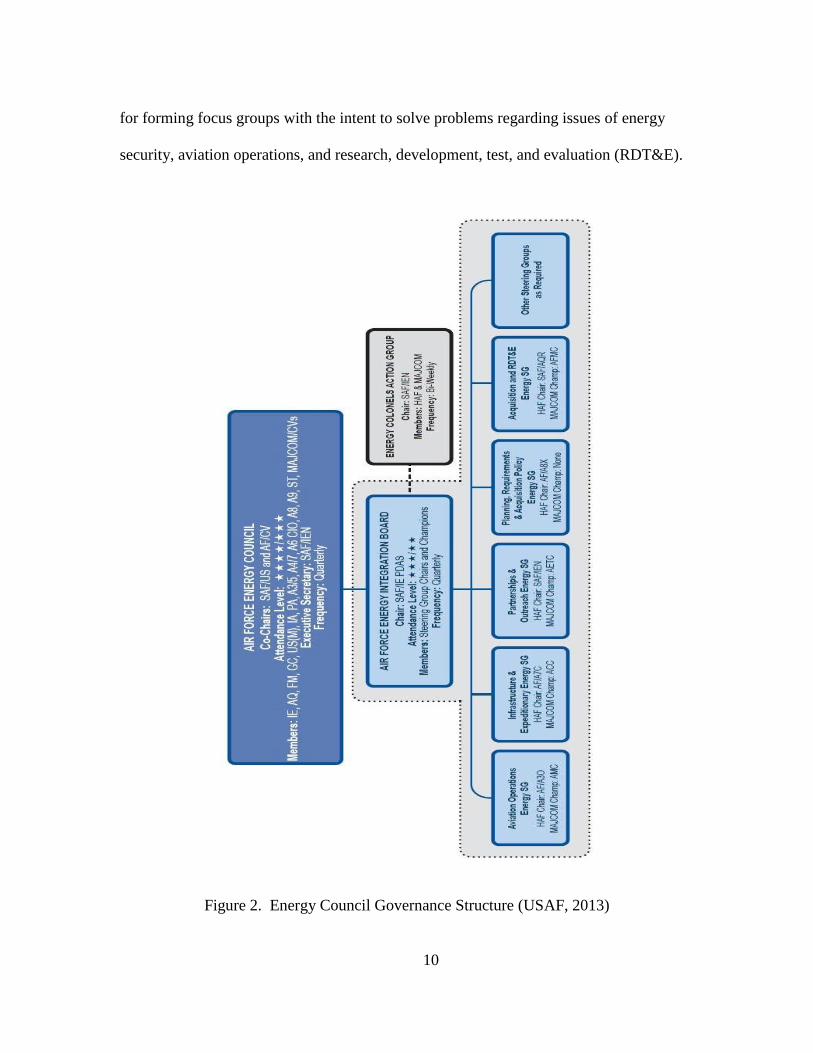
Energy Council. Figure 2 displays this three-tiered governing body, which is responsible

10

for forming focus groups with the intent to solve problems regarding issues of energy

security, aviation operations, and research, development, test, and evaluation (RDT&E).

Figure 2. Energy Council Governance Structure (USAF, 2013)

11

Research into photovoltaics (PV) can have a positive impact to supply assurance

while fulfilling public mandates and internal service objectives such as the increased

utilization of renewable energy sources. The protection of the U.S. power grid and, by

extension, vulnerability of power supplies on military installations has come into focus in

recent years. Adequate protection of these resources must be accomplished through

physical and cyber security methods.

Vulnerability of U.S. Grid

The federal budget, in alignment with DoD’s strategy to defend its networks and

U.S. interests from cyber-attacks, will attempt to fulfill the Cyber Mission Force of 133

teams tasked with cyber security by end of Fiscal Year (FY)18. Federal spending is

projected to be $6.7 billion in FY17, a 15% increase from FY16, in response to greater

cyber security threats (US Department of Defense, 2016).

In March of 2007, an experiment named “Aurora” was conducted to test the

resilience of U.S. energy assets by using computers to launch a cyber-attack on a

generator at the Department of Energy’s Idaho Laboratory. Experimenters were

successful in causing the generator to emit smoke, malfunction, and cease operation

(Meserve, 2007). This test highlighted the relative ease with which internal or external

forces could exploit the U.S. power grid and cause a local or potentially nationwide

power failure. A 2017 world-wide cyber-attack using ransomware, software that renders

computers inaccessible pending monetary payments to restore system access, renewed

concerns regarding U.S. power grid vulnerability. More than 57,000 infections in 99

countries were observed primarily targeting Microsoft Windows operating systems in

12

Russia, Ukraine, and Taiwan (Volz, 2017). The concern is not just for vulnerability of

civilian power, but also for the possible compromise of national defense should military

installations be targeted. As ransomware and similar software intended to exploit or

destroy become more sophisticated, the DoD is facing a situation prompting exploration

of alternative energy options to build a robust power supply network which minimizes

the likelihood of and the damage caused in the event cyber-attacks occur.

DoD Considerations

The issue of facility energy consumption has spurred additional legislation to

combat the increase in facility energy intensity. The years 2001 through 2006 saw a 40%

increase in Air Force energy consumption (AFCEC, 2014). The National Defense

Authorization Acts of 2007, 2008, and 2009; the Energy Policy of Act of 2005; and

Executive Order 13423 established the federal requirement for 7.5% utilization of

renewable energy by 2013 and 25% by 2025 for all federal and DoD facilities,

respectively (AFCEC, 2014; Energy Flight Plan, 2017). The U.S. Department of Energy

reports that, as of this writing, 8.3% of federal government energy consumption comes

from renewable sources (Office of Energy Efficiency & Renewable Energy, 2018).

Progress in meeting the DoD’s 25% goal remains to be seen. Future considerations

regarding vulnerability to attack, climate change, and increased demand will require

substantial effort to accommodate. With today’s resource constraints, photovoltaics may

provide an avenue to directly contribute to the Air Force’s pursuit of net zero energy on

installations by 2030 and fulfillment of the priority to increase integration of new

technologies to reduce costs while leveraging investments (USAF, 2013).

13

Photovoltaic Basics

PV panels convert sunlight into electricity through the use of thin layers of semi-

conducting material. The most common semi-conductor used for this purpose is silicon

metal, shown in Figure 3. Silicon-based panels are commercially available in several

varieties including monocrystalline, polycrystalline, thin-film, and amorphous. Other

semi-conducting material can be used for PV purposes but are not yet widely available or

fully tested. Although varying in cost and efficiency, all of these PV types operate under

the same basic principles. The most common panel positioning method is adjusting the

tilt angle toward the sun to capture direct radiation. Panels are also capable of capturing

indirect, or diffuse, radiation caused by airborne water vapor. Further information

regarding PV orientation, panel types, and basic principles of PV operation is covered in

the remainder of this section.

Figure 3. A chunk of semi-conducting silicon metal (WebElements, 2018)

14

Operating Principles

The most basic PV unit used to construct larger networks of panels is called a cell,

with each cell producing one to two watts of electrical energy (Office of Energy

Efficiency & Renewable Energy, 2013). Large arrays of solar cells can be connected in

series to produce the desired power output. This makes PV an option for large or small

power needs. PV panels, which are most efficient when their flat surface is positioned

normal to the sun, produce direct current (DC) which can be used or converted to

alternating current (AC) for most power needs such as residential housing. Figure 4

shows a simplified depiction of silicon’s arrangement of atoms and electrons, also known

as its crystal structure. Each group of dots, represents an atom of silicon (large dot) with

four valence electrons in each atom’s outer shell, thus resulting in a net neutral charge.

Figure 4. Simplified depiction of crystalline silicon (Laube, 2018)

To enable the silicon to conduct electricity for use in PV applications, impurities

are deliberately introduced (a process known as doping) to create an imbalance of

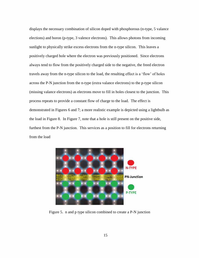
electrons resulting in a net-positive or net-negative charge (Laube, 2018). Figure 5

15

displays the necessary combination of silicon doped with phosphorous (n-type, 5 valance

elections) and boron (p-type, 3 valence electrons). This allows photons from incoming

sunlight to physically strike excess electrons from the n-type silicon. This leaves a

positively charged hole where the electron was previously positioned. Since electrons

always tend to flow from the positively charged side to the negative, the freed electron

travels away from the n-type silicon to the load, the resulting effect is a ‘flow’ of holes

across the P-N junction from the n-type (extra valance electrons) to the p-type silicon

(missing valance electrons) as electrons move to fill in holes closest to the junction. This

process repeats to provide a constant flow of charge to the load. The effect is

demonstrated in Figures 6 and 7; a more realistic example is depicted using a lightbulb as

the load in Figure 8. In Figure 7, note that a hole is still present on the positive side,

furthest from the P-N junction. This services as a position to fill for electrons returning

from the load

Figure 5. n and p type silicon combined to create a P-N junction

16

Figure 6. Post-photon strike on PV cell, electron freed

Note: (left to right) holes filled by other electrons. Notice the hole appears to travel away

from P-N junction as previous positions are occupied

Figure 7. freed electron flow

Figure 8. Electron flow, n-type SI, through load, back to p-type SI (TechyChaps, 2017)

17

Electrons flow through a circuit within a closed loop; therefore, as photons

continually bombard the silicon’s extra valance electrons free, they will flow through the

load and back to the positive side to fill in the rogue hole. This process is more easily

seen in Figure 8. The same principles are exploited regardless of specific PV application.

Several types of panels are available today that make use of these principles and are

discussed in the following section.

Panel Type

A sample of different PV types are displayed in Figure 9. Note that the

amorphous cell on the displayed calculator is visible on its upper right corner. These

panels differ in appearance, efficiency, and other attributes. Monocrystalline cells have a

more complicated, higher cost manufacturing process and result in about 15% efficiency

(National Energy Foundation, 2017). In other words, monocrystalline panels can convert

approximately 15% of the sunlight striking it to electricity. Polycrystalline, or

multicrystalline, cells are slightly cheaper than monocrystalline ones due to a simplified

manufacturing process and a lower efficiency of approximately 12% (National Energy

Foundation, 2017). Approximately 85% of the U.S. PV market is comprised of the

crystalline variety (Maehlum, Which Solar Panel Type is Best? Mono- vs. Polycrystalline

vs. Thin Film, 2017). Their availability combined with higher demonstrated efficiency

makes them the mostly likely candidate for any given PV application (Nagangast,

Hendrickson, & Matthew, 2013). Thin-film silicon is another option which comprises

11% of market penetration and can achieve up to 20.4% efficiency depending on the

type. The most common type is amorphous silicon (a-Si), which has an efficiency of

18

13.4% and higher manufacturing cost, thus making it a sensible option for small, low-

power applications such as calculators (Maehlum, 2015). Other variations of thin-film

technology are cadmium telluride (CdTe) and copper indium gallium selenide

(CIS/CIGS), which are currently emerging technologies with higher efficiencies and

expected market share growth (Maehlum, 2015; Mekhile, Saidur, & Kamalisarvestani,

2012). Studies involving non-crystalline panel technologies have yielded significant

discrepancies between resulting performance models (Cameron, Boyson, & Riley, 2008)

Due to the significantly lower market share of non-crystalline technologies and limited

research budgets, these panel types are not used in this research, which instead focuses on

commercially abundant crystalline panels.

Note: Monocrystalline (upper left), polycrystalline (upper right), thin film (lower left),

and amorphous (lower right) PV cells

Figure 9. Various PV types (Maehlum, 2017)

Sandia National Laboratories has conducted studies to validate existing PV

performance models and produce an annual model accounting for the non-proportional

output of PV panels comprised of different technologies. Primary emphasis was placed

on models that are readily available through a number of U.S. Department of Energy

19

(DoE)-sponsored calculation tools such as Solar Advisor Model (SAM), PVWATTS,

PVFORM, and PVMod. One-year studies were conducted on three different test systems

installed without shading and at latitude tilt; the first two systems, utilizing 210 and 220

watt panels, respectively, were comprised of five in-series crystalline silicon panels

connected to a 2 kW inverter. The third system contained two strings of seven silicon

panels connected to a 2.5 kW inverter. These systems were used to validate radiation,

panel output, and inverter output performance submodels in the calculation tools

mentioned previously. The results were conclusive for crystalline technologies, showing

modeled and experimental results were in agreement within a margin of 3%. Non-

crystalline technologies, such as thin-film, showed significant disagreement between

models (Cameron, Boyson, & Riley, 2008). As previously mentioned in Chapter I, the

effect of tilt angles was not studied. This necessitates further study to validate or produce

new models to predict PV performance with a horizontal tilt. For these reasons, current

research focuses on evaluating the crystalline variety placed flat on a surface.

Panel Orientation

The most efficient currently known method of capturing sunlight is exposure to

direct rays by positioning panels normal to incoming photons. Global latitude is the

primary piece of positional data that dictates optimal tilt angle of PV panels for maximum

electricity-producing efficiency (Landau, 2015). However, emerging data suggests that

horizontal panels (zero degree tilt angle) may perform more efficiently than conventional

systems in overcast conditions because of their greater exposure to diffuse irradiance.

This insight has spurred current research to explore the potential of utilizing horizontal

20

PV technology for new applications within regions where solar irradiance is not optimal

for traditional PV installation (Brusaw & Brusaw, 2016). In addition, a study was

conducted to explore the performance impact of different sun tracking systems (Koussa,

Haddadi, Saheb, Malek, & Hadji, 2012). Researchers tested two fixed panel, two single

rotating axes, and one two-axis system and calculated the amount of direct, diffuse, and

reflected solar irradiance encountered by each. The five configurations were used in the

hot and dry Algerian desert to determine and compare power outputs from each of the

five systems. As expected, the ability of panels to capture direct beam irradiance was

affected by different trackers. Interestingly, it was also found that cloudy days yielded

the same power output regardless of the presence of a sun-tracking system. Further,

horizontal PV panels performed best during completely cloudy days when compared to

inclined, one-axis and two-axis sun tracking systems. Further evidence of increased

horizontal panel output on cloudy days has been observed. The observations were made

by a U.S.-based company specializing in design and testing of a proprietary PV product

utilizing horizontal PV cells. These cells are embedded between tempered glass to

produce a potential alternative to traditional pavement. This product provided the

impetus for this research and is discussed in the following section.

Photovoltaic Pavement Systems

Military installations are far from suffering a shortage of sidewalks, streets,

parking lots, and other pavement. The emergence of PV pavement systems may have the

potential to out-produce conventional systems through sheer amounts of area available

for PV coverage. One U.S.-based company, Solar Roadways, Incorporated (SRI) is

21

currently conducting test and evaluation of their product which consists of assembled

hexagonal units containing 48W silicon-based solar cells embedded between tempered

glass and polymer insulation. A sample of the product is displayed in Figure 10. The

product also features other capabilities such as self-heating, light-emitting diodes (LED)

to replace road paint, and integrated drainage (Brusaw & Brusaw, 2016). The PV units

are intended to be placed on a flat surface which raises questions as to their efficiency

and ability to effectively generate electricity.

Figure 10. SRI's product - photovoltaic pavement system (Brusaw & Brusaw, 2016)

Performance testing is being conducted using store-bought silicon panels. Each

of three test sites, the latest of which is located at the Missouri Department of

Transportation as of March 2016 and shown in Figure 11, is equipped with one flat panel

and one angled panel to compare variation in results. The first test site was installed in

April 2015 at the Biosphere 2 in Oracle, Arizona, while the second test site was installed

22

in August 2015 at SRI’s facility in Sagle, Idaho. The first public test of this product has

been taking place since late 2016 in Sandpoint, Idaho, shown in Figure 12. Preliminary

analysis of PV performance data collected at different latitudes suggest that flat panels

generate more electricity than tilted panels during overcast conditions (Brusaw &

Brusaw, 2016). Additionally, total monthly energy produced is comparable between the

tilted and horizontal panels. Table 1 displays the most recent results from the Arizona

site in which outputs from each panels appear almost the same. Similar results are

provided for the other test sites.

Figure 11. Test site at Missouri DOT (Brusaw & Brusaw, 2016)

23

Figure 12. First public test in Sandpoint, Idaho (Fingas, 2016)

Table 1. One year of test data in Oracle, AZ

24

It is hypothesized that the similar results are caused by the scattering of photons

through airborne water vapor, thus allowing for easier harvesting of diffuse radiation by

flat panels than angled panels. Successfully replicating this data for a variety of latitudes

and climate conditions may prove the PV pavement application feasible for installations

without sufficient sunlight to justify investing in a PV array which is intended to capture

direct beam sunlight. Prior research has been conducted by Nussbaum (2017) to

determine the applicability of PV panels for energy production on DoD installations. His

study provided the foundation for further research into the potential application of

horizontal PV on DoD installations through the methodical selection of test locations for

horizontal PV systems.

Global Position and Climate Types

The Köppen-Geiger Climate Classification system is used to divide the globe into

five main climate zones as shown in Figure 13. The system further divides each zone

into a multitude of varying climate types. Previous research utilized this system to

ascertain variance in environmental factors affecting PV performance. These factors are

largely dependent on latitude, temperature, humidity, and changes in air mass

(Nussbaum, 2017). Statistical analysis of 1,763 Air Force installations placed them into

bins representing latitude and longitude. From this analysis, 25 regions were identified in

which PV system performance could be measured to represent latitudinal and

longitudinal effects of temperature and humidity. These regions are listed in Table 2.

Subsequent Pareto analysis, a statistical technique used to select principle components

that produce the greatest overall effects on performance, established the regions in which

25

test systems should be placed to gather performance data representing the entire set of

installations. As of this writing, concurrent research at AFIT uses this classification

system to perform logistical regression based on the interactions between global position

and climate types. Additionally, the Air Force operates installations in tropical, dry,

temperate, and boreal climate types. Consequentially, the polar climate type will not be

included in this round of research.

Note: A-Tropical, B-Dry, C-Temperate, D-Boreal, E-Polar

Figure 13. Köppen climate types (Beck, Grieser, & Rubel, 2005)

26

Table 2. Climate types and locations analyzed (Nussbaum, 2017)

27

Temperature and Humidity Performance Models

Many competing equations exist describing efficiency and power output as

functions of temperature. Functions that utilize ambient temperature yield more variance.

As shown in Tables 3 and 4, respectively, there are currently 24 functions describing

efficiency and 27 describing power (Skoplaki & Palyvos, 2008; Rosell & Ibanez, 2006).

Global research is first intended to center on the effects of temperature and humidity on

mono- and poly-crystalline PV panels to refine existing performance models using

empirical data. Humidity has been shown to have a substantial direct and indirect

influence on PV performance. Directly, visible and microscopic water droplets divert

incoming photons through refraction, diffraction, and reflection. Indirectly, dust build-

up, in significant amounts, creates a barrier to photons striking the doped silicon within

the PV panels and thus reducing power output. It is estimated that between 1 and 65.8

percent of potential PV output is lost due to these effects, directly depending on the

percentage of solar rays blocked (Mekhile, Saidur, & Kamalisarvestani, 2012).

Existing models for predicting the performance of PV panels have been produced

by Sandia National Laboratories and are supported by the U.S. Department of Energy

(DoE) (Cameron, Boyson, & Riley, 2008). Further validation and refinement of these

models has been conducted to improve the accuracy of predictions against empirical

results. Typical tests are concerned with panels tilted at latitude and toward the sun for

maximum energy output.

Additional modeling efforts in sunny and cloudy conditions have included the

panel fill factor (FF) in addition to short-circuit current, open-circuit voltage, and

maximum power output as variables dependent on solar intensity and model temperature.

28

The findings confirm weather’s strong influence on irradiance captured by PV (Wei,

Yang, & Fang, 2007). Most of the research requires humidity as an independent variable

in their respective performance models while all require temperature. Refining these

functions for PV system performance will allow users to determine the optimum size of

the system for specific load requirements under local meteorological conditions.

Table 3. Competing Temperature/Efficiency Equations (Skoplaki & Palyvos, 2008)

29

Table 4. Competing Temperature/Power Equations (Skoplaki & Palyvos, 2008)

30

The cited study which determined optimal sun-tracking configuration used only

one proposed model predicting PV behavior and is described by the equation,

where q is the charge on an electron (1.602 ×10-19 C), k is Boltzmann’s constant

(1.381×10-23 J/◦K), Tc is the solar cell temperature, I is the operating current (A), V is the

operating voltage (V), IL is the photocurrent, and I0 is the diode reverse saturation current.

The γp and Rs factors are the empirical photovoltaic curve fitting parameter and model

series resistance, respectively (Koussa, Haddadi, Saheb, Malek, & Hadji, 2012). Note

that humidity does not appear in this model, although previously cited data suggests

humidity significantly affects the PV’s ability to capture diffuse solar radiation. To

properly utilize horizontal PV systems, especially in regions with little sunlight and

persistently overcast conditions, capturing the maximum amount of diffuse radiation is

paramount. Therefore, a performance model that can accurately predict power output as

functions of temperature and humidity is necessary to ascertain the feasibility of using

horizontal orientation at any global location.

31

III. METHODOLOGY

Little research has been done with respect to horizontal photovoltaic (PV) panels

and current research is inspired by existing methods of data collection and analysis

covered in Chapter II. Since this line of research builds upon a prior feasibility study, the

methods for data collection and selection of test sites have already been established. Test

system design and prototyping was conducted by a team of AFIT graduate students while

this phase of the research carried out manufacturing and distribution of the systems while

maintaining working relationships with points of contacts monitoring data collection in

the field. The following sections will provide details regarding panel selection, test

system manufacturing and distribution, and analysis techniques. Due to the amount of

detail and meticulous planning required for the research, mistakes were likely to occur

and will be explained in this chapter as potential sources of error.

Test System Design, Manufacture, and Distribution

The primary targets of this study were two types of silicon-based PV panels:

monocrystalline and polycrystalline. These panel types are commercially available off-

the-shelf, which make them the most likely candidates for use in any given PV

application. Further research may concern itself with thin-film PV or other emerging

technologies. These crystalline panels produce the same amount of electricity per rated

watt, although monocrystalline is slightly more space efficient. For the sake of

thoroughness, both types are included to ascertain any differences in the effects of

temperature and humidity between the two types. For each test system, one 50W

polycrystalline panel and one 25W monocrystalline panel are included.

32

Each control unit, as shown in Figure 14, is equipped with a temperature/humidity

probe to collect measurements of primary factors, a satellite communications uplink, and

a central processing unit (CPU) for central control of peripheral devices. Sensitive

electronic equipment is protected from the elements within a robust Pelican™ case.

Panels are equipped with power-monitoring circuits shown in Figure 15. These devices

transmit data via a CAT5e network cable to the CPU for storage.

Figure 14. Control unit housing

33

Figure 15. Power-monitoring circuit

Ambient temperature, humidity, and power output measurements are made every

15 minutes and contain 64 distinct voltage and current readings within each interval.

Each measurement is then stored on a Micro SD flash memory card for later retrieval and

submission to researchers. Additionally, data submissions are requested to be ideally

made at the end of each month to maintain a steady influx of data for compilation for

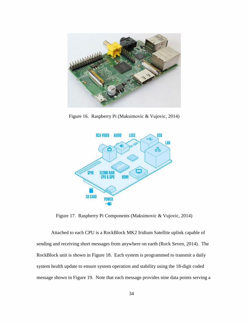
future analysis. The CPU used for this system is a Raspberry Pi, displayed in Figure 16,

which is a standard operating computer containing typical components such as random

access memory (RAM), graphics processing unit, and peripheral connections

(Maksimovic & Vujovic, 2014). The CPU interface is conducted using a standard

keyboard for command entry and display monitor. Figure 17 shows the different

available components such as SD flash memory card port, USB, Local Area Network

(LAN) connection, audio/video capability (HDMI included), and LED status indicators.

34

Figure 16. Raspberry Pi (Maksimovic & Vujovic, 2014)

Figure 17. Raspberry Pi Components (Maksimovic & Vujovic, 2014)

Attached to each CPU is a RockBlock MK2 Iridium Satellite uplink capable of

sending and receiving short messages from anywhere on earth (Rock Seven, 2014). The

RockBlock unit is shown in Figure 18. Each system is programmed to transmit a daily

system health update to ensure system operation and stability using the 18-digit coded

message shown in Figure 19. Note that each message provides nine data points serving a

35

specific purpose to allow researchers to verify system status. In order, they are mean

ambient temperature in degrees Celsius, mean ambient humidity, average daily power

produced by each panel, operating voltages on both panels, panel node temperatures, and

motherboard temperature.

Figure 18. RockBlock MK2 (Rock Seven, 2014)

Figure 19. System health update (Nussbaum, 2017)

36

The control units are not self-powered and require an external 110-240V, 50-60

Hz power source for operation. Sites are required to connect their respective unit to a

prime power source or use a standalone battery provided by researchers prior to the start

of the study. Five of the 37 test sites required a battery as a power source due to

limitations in authorized placement locations for the systems combined with lack of

available prime power source. The chosen battery type and accompanying control unit is

a 12V, 12ah, sealed lead acid battery purchased from AA Portable Power Corporation.

These units come equipped with a DC control unit and provide a stable DC power source

for the test system. The battery and DC controller are displayed in Figures 20 and 21.

They are recharged via an additional 30W mono-crystalline PV panel. A complete

system set-up with battery power source and charging PV panel is displayed in Figure 22.

Figure 20. 12V 12Ah battery with DC controller (AA Portable Power Corp, 2017)

37

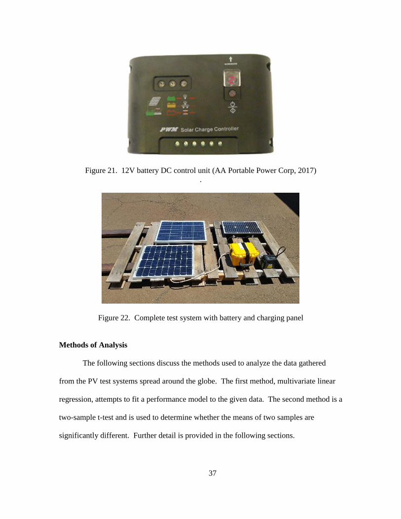
Figure 21. 12V battery DC control unit (AA Portable Power Corp, 2017)

.

Figure 22. Complete test system with battery and charging panel

Methods of Analysis

The following sections discuss the methods used to analyze the data gathered

from the PV test systems spread around the globe. The first method, multivariate linear

regression, attempts to fit a performance model to the given data. The second method is a

two-sample t-test and is used to determine whether the means of two samples are

significantly different. Further detail is provided in the following sections.

38

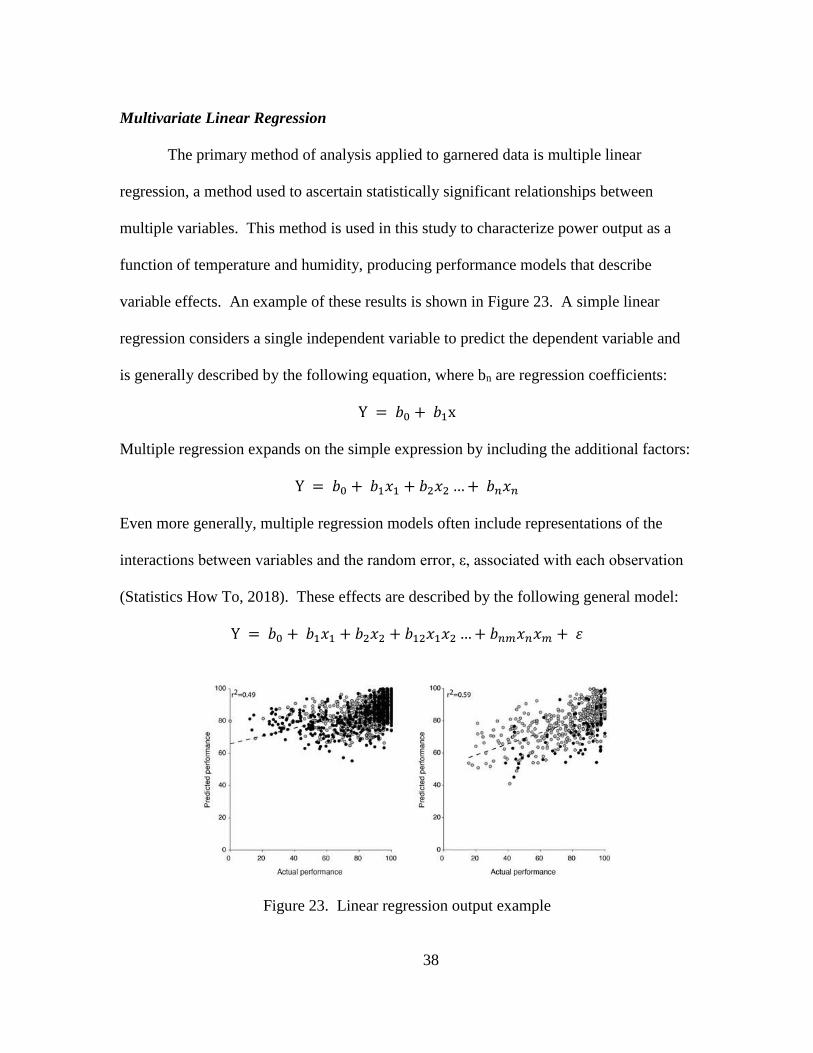
Multivariate Linear Regression

The primary method of analysis applied to garnered data is multiple linear

regression, a method used to ascertain statistically significant relationships between

multiple variables. This method is used in this study to characterize power output as a

function of temperature and humidity, producing performance models that describe

variable effects. An example of these results is shown in Figure 23. A simple linear

regression considers a single independent variable to predict the dependent variable and

is generally described by the following equation, where bn are regression coefficients:

Y = 𝑏0 + 𝑏1x

Multiple regression expands on the simple expression by including the additional factors:

Y = 𝑏0 + 𝑏1𝑥1 + 𝑏2𝑥2 … + 𝑏𝑛𝑥𝑛

Even more generally, multiple regression models often include representations of the

interactions between variables and the random error, ε, associated with each observation

(Statistics How To, 2018). These effects are described by the following general model:

Y = 𝑏0 + 𝑏1𝑥1 + 𝑏2𝑥2 + 𝑏12𝑥1𝑥2 … + 𝑏𝑛𝑚𝑥𝑛𝑥𝑚 + 𝜀

Figure 23. Linear regression output example

39

The aim is to model each panel type separately with power output being the sole

dependent variable in their respective models. Since the two panel types are of different

sizes, the polycrystalline panel being double the size of the monocrystalline, each power

output reading was converted into wattage per square foot of area. The independent

variables considered are the month, season, latitude, longitude, humidity, ambient

temperature, internal control system temperature, and respective node temperatures. Also

included is a factor indicating daylight hours for the purpose of excluding night data from

the analysis. This factor is calculated from sunrise and sunset data obtainable from the

website owned by the Astronomical Applications Department of the U.S. Naval

Observatory ( Astronomical Applications Department, 2016). As a reminder, a node

consists of a PV panel and its attached power-monitoring circuit. Interactions between

independent variables may result in collinearity, which is typically a disqualifier for

inclusion. Multivariate regression assumes the absence of this effect, along with a few

other key assumptions (Statistics Solutions, 2018).

The first assumption required to conduct a multivariate regression is a linear or

curvilinear relationship between variables which can be observed using scatterplots.

Second, multivariate normality is assumed to ensure residuals of the regression follow a

normal distribution. Histograms or goodness of fit tests (Kolmogorov-Smirnov, Shapiro-

Wilks, etc.) can be used to assess normality. The third assumption is lack of

multicollinearity, which occurs when independent variables are highly correlated with

each other. These can obscure principle components that explain variance in dependent

variable observations and should be filtered out. The final assumption is

40

homoscedasticity of the data, which indicates error variances are similar across

independent variables and can be checked for using a scatterplot of residuals against

predicted values. Non-equal distribution of residuals indicates heteroscedasticity and

would necessitate a non-linear transformation, introduction of a quadratic term, or other

remedial technique to aid analysis. Verifying the key assumptions allows the application

of multivariate linear regression. Multiple models are likely required to account for

differing panel types, latitudes, or other unforeseen variables. Further, test site monitors

may place their systems on different surfaces and at varying elevations. To control for

these possible discrepancies, multiple test systems are placed in the same location, within

one mile of each other, to collect measurements for variance testing.

Variance Testing

Testing for variance using three or more systems, as originally planned, would

requires an analysis of variance (ANOVA) to check for significant variation between

outputs from multiple systems. However, due to system error on one of the home

systems, only two of the systems are analyzed to ascertain variance in differing surfaces.

Therefore, a two-sample t-test is conducted to determine any significant difference in the

independent sample means. This process ensures any variance in power output between

the differing surface types has minimal interference with the temperature/humidity study.

The two independent samples being examined are from a ground-level pavement surface

and a rooftop system. Follow-on research will attempt to ensure all three systems are

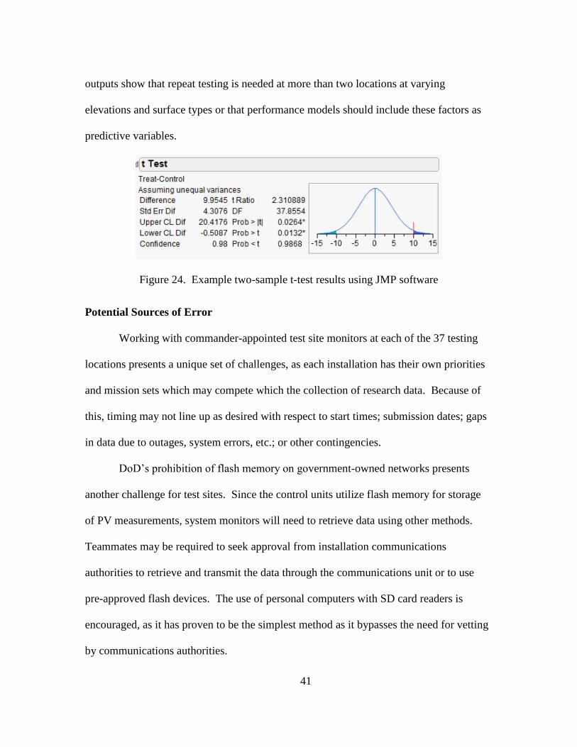
functional for a thorough variance test. A two-sample t-test sample output using JMP

statistical analysis software is shown in Figure 24. Significant deviations between the

41

outputs show that repeat testing is needed at more than two locations at varying

elevations and surface types or that performance models should include these factors as

predictive variables.

Figure 24. Example two-sample t-test results using JMP software

Potential Sources of Error

Working with commander-appointed test site monitors at each of the 37 testing

locations presents a unique set of challenges, as each installation has their own priorities

and mission sets which may compete which the collection of research data. Because of

this, timing may not line up as desired with respect to start times; submission dates; gaps

in data due to outages, system errors, etc.; or other contingencies.

DoD’s prohibition of flash memory on government-owned networks presents

another challenge for test sites. Since the control units utilize flash memory for storage

of PV measurements, system monitors will need to retrieve data using other methods.

Teammates may be required to seek approval from installation communications

authorities to retrieve and transmit the data through the communications unit or to use

pre-approved flash devices. The use of personal computers with SD card readers is

encouraged, as it has proven to be the simplest method as it bypasses the need for vetting

by communications authorities.

42

IV. ANALYSIS AND RESULTS

The aim of this chapter is to perform all necessary analysis to obtain an accurate

performance model characterizing the behavior of monocrystalline and polycrystalline

photovoltaic (PV) panels in each zone enumerated in Table 2. The test zone

identification process discussed in the previous chapter allowed for selection of U.S.

military installations and appointment of site monitors to install, monitor, and transmit

data from their respective test systems. This chapter begins with an explanation of the

amount and quality of data garnered from installations participating in the study and then

breaks down the results of relevant analyses. First, global models are sought that predict

behavior across the earth. New models are then obtained for four of the five existing

Kӧppen climate types. As a reminder, this is because the Air Force does not operate in

polar climate, thus there are no available test sites. Finally, site-specific expressions are

provided to identify regions where ambient temperature and humidity have the most

effect on power output. The chapter concludes with comparisons of resulting models

with existing performance models discussed in the review of the literature.

Data Quality

Power performance data was obtained from 25 of the 37 test locations. Those

sites that were not able to transmit data faced various issues with priority, setup, systems

errors, or availability of power. All test locations are shown in Table 5, which is

analogous with Table 2. In addition, Table 6 lists each participating location and its

respective Kӧppen climate type.

43

Table 5. Test Site participation

Table 6. Analyzed test locations and their corresponding Kӧppen climate types

Region Actual Latitude Actual Longitude Site Name Owning Installation of Record

A 20.890247 -156.4447 KAHULUI COMMUNICATION STATIONKEAUKAHA MIL RESERVATION

C 12.187654 -68.970935 CURACAO SITE # 1 - Aruba DAVIS MONTHAN AFB

D 11.5183 43.0672 CHABELLEY USAFE-AFAFRICA

E -22.219846 114.103057 LEARMONTH AF SOLAR OBSERVATORYYOKOTA AB

G 32.8888 -106.1038 HOLLOMAN SITE # 1 HOLLOMAN

G 29.12 -100.48 LAUGHLIN AFB AUX 1 SITE # 1 LAUGHLIN AIR FORCE BASE

G 34.39 -103.32 CANNON AFB SITE # 1 CANNON AIR FORCE BASE

G 33.904322 -117.262814 MARCH AFB SITE # 1 MARCH AIR RESERVE BASE

H 31.1833 -92.632 CLAIBORNE AIR FORCE RANGE SITE # 1BARKSDALE AIR FORCE BASE

H 26.983 -80.108 JONATHAN DICKINSON MISSILE TRACKING PATRICK

I 34.5901 32.9892 RAF AKROTIRI RAF AKROTIRI

J 33.581778 130.448329 ITAZUKE AUXILIARY AIRFIELD SITE # 1YOKOTA AB

L 41.0508 -112.9356 UTTR - NORTH SITE # 1 HILL AFB

L 41.13 -95.75 OFFUTT FAMILY HOUSING ANNEX SITE # 1OFFUTTAIRFORCEBASE

L 38.16 -121.56 TRAVIS ILS OUTER MARKER ANNEX SITE # 1TRAVIS AFB

L 38.82 -104.71 PETERSON AFB SITE # 1 PETERSON AFB

L 38.95 -104.83 U S A F ACADEMY SITE # 1 U S A F ACADEMY

L 41.1517 -111.9922 SO WEBER ENVIRONMENTAL ANNEX HILL AFB

M 40.66807 -86.14765 GRISSOM AIR FORCE BASE SITE # 1 GRISSOM ARB

M 37.08 -76.37 LANGLEY AFB SITE # 1 JBLE

M 40.026986 -74.584263 MCGUIRE AFB JB MDL

M 44.89 -93.2 MINN-ST PAUL SITE # 1 MINN-ST PAUL

N 38.7754 -27.0891 LAJES FIELD SITE # 1 LAJES FIELD

O 37.753755 127.027811 CAMP RED CLOUD COMMUNICATION OSAN

O 37.08 128.59 OSAN SITE # 1 OSAN AB

P 55.245335 -162.770084 COLD BAY LONG RANGE RADAR SITEEARECKSON AS

Q 47.7947385 -101.2979626 MINOT AF MISSILE SITE D1 SITE # 1 MINOT AFB

Q 47.11439 -122.573129 CAMP MURRAY AGS SITE # 1 CAMP MURRAY AGS

Q 48.418476 -101.338604 MINOT AFB SITE #1 MINOT AFB

Q 47.52 -111.18 MALMSTROM SITE # 1 MALMSTROM AFB, MT

R 46.933892 -67.911875 DFAS ANNEX - Limestone Maine WHITEMAN

S 50.0166 6.7704 GROSSLITTGEN WATER SYSTEM ANNEX SPANGDAHLEM

T 52.729239 174.099627 EARECKSON AS SITE # 1 EARECKSON AS

U 64.2852 -149.1515 CLEAR AIR FORCE STATION SITE # 1 CLEAR AIR FORCE STATION

U 65.564961 -167.967703 TIN CITY LONG RANGE RADAR SITE EARECKSON AS

W 76.53 -68.7 THULE AIR BASE SITE # 1 THULE AIR BASE

X 58.905625 5.7215649 STAVANGER ADMIN OFFICE SITE # 1 RAF ALCONBURY

44

Note that data garnered from installations are highlighted in green. Several

locations were able to install and begin data transmissions as early as May, 2017. Of the

locations that submitted data, the latest test start date covered the month of October,

2017. As of this writing, these 25 systems are still operating. They will continue the

study into the following year with the other 12 test sites working to address various

technical or installation issues including battery malfunction, component failure, faulty

data, or anchoring system problems. All test systems, with the exception of three systems

sent to the Alaskan zone installations, were confirmed by site monitors as received and

intact. These are expected to join the study early in 2018. Inclusion of more systems into

the study will yield more data and hone the accuracy of resulting performance models.

Performance Modeling

Multiple linear regression was performed using JMP Pro Statistical Analysis

Software, Version 12.0.1, 64-bit edition by SAS Institute Inc. The aim was to

characterize each panel type separately as the difference in material type may be

influenced by environmental factors in unforeseen ways. Fitting the data to a linear

model requires testing the key assumptions for multivariate linear regression outlined in

chapter III to ascertain whether non-linear analysis techniques or transforms are

necessary. A best model for each panel type is then selected that allows a reasonable

prediction of energy output at locations with wide distributions of temperature and

humidity. Varying accuracy prompted additional models applicable to respective climate

types and specific locations around the world. The effect each predictor had on the

power output and coefficient of determination (R2) accuracy depends heavily on the

45

location, alluding to a high probability of additional location or region-specific predictors

affecting the power output of PV panels. Following initial experimentation with global

models, a new factor was introduced to delineate between the five Kӧppen climate types

(tropical, dry, temperate, boreal, and polar) and enable the creation of new models that

pertain to each climate type and provide more accurate characterization. Note that in

some models, the response variable is the logarithm of power output. In an effort to

improve the models and account for additional variance, Y and X value transformations

were used to linearize the models, create constant variance in the plot of residuals against

predicted values, and create a linear relationship with predictor variables. The five

transformations listed in Table 7 were used on response and predictor variables to find

the best fitting model. The best result for all models used a square root, logarithmic, or

no transform to linearize Y-values. Finally, multiple regression assumes that the

independent variables are not highly correlated with each other. This assumption is

tested using Variance Inflation Factor (VIF) values. As a general rule, VIFs greater than

10 indicate problematic collinearity between variables (Statistics Solutions, 2018).

Table 7. Transformations of Y to improve model performance (Buro, 2018)

46

Key Assumptions

Confirmation of model validity is first tested on the performance of the

monocrystalline panels, followed by the polycrystalline panel. A linear relationship

should be shown between each panel type and the independent variables. The

scatterplots for select locations in Figure 25 show one-to-one relationships between

power output and the independent variables of ambient temperature and humidity. It can

be seen from the scatterplots that knowledge of these factors alone does not allow an

accurate prediction of power output. Regardless, there is indication of a positive trend for

ambient temperature while humidity shows a negative trend. Interactions with other

factors likely explain the remaining variance in observations. Similar relationships are

shown for polycrystalline panel performance in Figure 26, though it appears the

independent variables are more correlated with power output for this material type.

Figure 25. Monocrystalline correlations at select locations, strong and weak examples

47

Figure 26. Polycrystalline correlations at select locations, strong and weak examples

Monocrystalline Models

The first model attempted to characterize temperature and humidity across all

ranges of latitude and longitude. Key assumptions for linearity were met, though the

result was unsatisfactory with an R2 value of 0.3111, indicating that only 31.11% of the

variation in the response is explained by the presence of these predictive variables. The

dependent variable y describes the power output in watts(W), Lt is the latitude, Ln is the

longitude, t is the ambient temperature, and h is the humidity. The global performance

model for monocrystalline PV panels is described by the following:

ln 𝑦 = 0.012𝐿𝑡 − 0.004𝐿𝑛 + 0.015𝑡 + 0.003(𝐿𝑡 − 40.691)(𝑡 − 32.77)

+ 0.001(ℎ − 36.059)(𝑡 − 32.77) + 0.465

48

Goodness-of fit tests can be conducted. However, due to such large sample sizes,

there is great sensitivity in tests for normality and failing them does not necessarily mean

a linear model cannot be created (Ghasemi & Zahediasl, 2012). A visual inspection of

the residual distribution histogram confirms the data is approximately normal and

analysis can continue unabated. Validity of the model and the linear relationship with

predictor variables are seen are seen in Figures 27 (top right) and 28, respectively. In

addition, the resulting VIF values indicate no issues with collinearity among the predictor

variables. The low R2 value may not be accurate enough to base decisions on, but it is

significant enough that the predictors should definitely be kept and supplemented with

additional predictors to hone accuracy. The histogram in Figure 27 shows

underestimations for the majority of predictions and overestimates concentrated in a

specific small range. This spike in overestimates may stem from location or region-

specific conditions. Location-dependent model accuracy, discussed in a later section,

confirms that residual values are expected to concentrate in different areas of the

histogram. In addition, linearity with predictor variables was vastly improved by using a

logarithmic data transformation compared to the non-transformed, cone-shaped values in

Figure 29. Subsequent performance models are provided without the full analyses in this

chapter. For the analyses of remaining global and climate-based models, comparable to

the one provided in Figures 27 and 28, see the appendix.

49

Figure 27. Monocrystalline global model, R2 = 0.3111

Figure 28. Post-transformation residual plots with predictors indicating linearity

50

Figure 29. Cone-shaped residual pattern indicating non-linearity

The boreal climate type is the first of the four climate types in which a model is

built. Experimentation with transformation functions from Table 7 and observance of

model diagnostics indicate a logarithmic Y-transform is the most appropriate, yielding

the highest correlations with ambient temperature and humidity. The power output in

boreal climate is described by the following equation:

ln 𝑦 = 0.229𝐿𝑡 − 0.028𝐿𝑛 − 0.006(𝐿𝑡 − 42.306)(𝐿𝑛 + 90.423) + 0.019𝑡

+ 0.0003(𝐿𝑛 + 90.423)(𝑡 − 33.283) + 0.00007(𝐿𝑡

− 42.306)(ℎ − 31.724)(𝑡 − 33.283) − 11.293

The result shows a significant predictive relationship between predictors and

power output for this climate type with an R2 value of 0.6120. The dominant variables

are latitude; longitude; ambient temperature; humidity; and interactions between latitude

and longitude, longitude and temperature, and latitude with humidity and temperature.

The clustering seen occurring on the plot of observed versus predicted values correspond

51

to different test locations, a predictable result given the various R2 accuracies among

locations. Similar results are seen in the residual histogram. Effects of individual

predictors are better seen in the location-specific models, though significance of

coordinate effects indicate missing predictor variables that describe local or regional site

conditions needed to obtain performance model accuracy.

The next climate type test is dry climate. The Y-transform used for linearizing

dry climate types outputs is the square root of the dependent variable. The power output

for monocrystalline PV in the dry climate type is given by the following:

√𝑦 = −0.002𝐿𝑛 − 0.006(𝐿𝑡 − 27.673)(𝐿𝑛 + 28.359)

+ 0.002(𝐿𝑡 − 27.673)(ℎ − 20.757) + 0.05𝑡 − 0.0002(𝐿𝑛

+ 28.359)(𝑡 − 39.006) − 0.527

Obtaining any accuracy with this particular model was difficult as was correcting

linearity by applying a square root transform. The equation describing dry climates, with

an R2 value of 0.3044 and a tendency to underestimate power output predictions, contains

environmental factors not explicitly identified but encapsulated by changes in latitude

and longitude. These unknown components are seen interacting with ambient

temperature and humidity. The resulting bivariate graphs show a linear relationship is

maintained between power output and the independent variables.

The temperate climate model utilizes the same data transform as the dry climate

model and acheives a slightly greater accuracy with an R2 value of 0.4109. The power

equation is as follows:

52

√𝑦 = 0.0006(𝐿𝑡 − 43.048)(𝐿𝑛 + 90.666) + 0.002(𝐿𝑡 − 43.048)(ℎ − 37.108)

+ 0.021𝑡 − 0.015(𝐿𝑡 − 43.048)(𝑡 − 32.616)

+ 0.0001(𝐿𝑡 − 43.048)(ℎ − 37.108)(𝑡 − 32616) + 2.673

Variation in power output appears to be relatively even between all locations

encompassed by the temperate category, evidenced by the lack of clustering and

relatively even number of residuals on either side of the best fit line.

The final climate model is tropical. It was found that a logarithmic transform

yielded the greatest accuracy for tropical climates, unlike, dry, and temperate. Accuracy

is second highest to the boreal model with an R2 value of 0.5472. The power output is

given by the following equation:

ln 𝑦 = −0.422𝐿𝑛 − 13.977ln ℎ − 13.18 ln 𝑡 + 0.118(𝐿𝑛 + 76.153) ln 𝑡

+ 3.69 ln ℎ ln 𝑡 + 19.253

Significant clustering on the residuals histogram is evident, showing differences

in specific locations that affect accuracy along with a more severe tendency to

underestimate power predictions. The bivariate fit at the bottom of the figure, with

exception of a few data points, maintains that there is linear relationship between power

and the predictor variables of interest, temperature and humidity. It is thought that

inclusion of additional factors, to be discussed in more detail during researcher

recommendations, will help refine each model’s accuracy.

53

Polycrystalline Models

The following models describe the effects of ambient temperature and humidity

using polycrystalline PV panels. The same analyses are again conducted, first attempted

for a global characterization and then on the four Kӧppen climate types. Polycrystalline

material appears to behave slightly differently, requiring different data transforms to

obtain the most accurate models. The global model utilized a square root transform,

though validity is highly suspect with an R2 value of 0.2166. The global power output is

given by the following equation:

√𝑦 = −0.004ℎ + 0.05𝑡 + 0.0002(ℎ − 39.096)(𝑡 − 31.745) + 0.01𝐿𝑡 + 0.002𝐿𝑛

+ 2.035

Additional factors are definitely necessary to refine this model. The boreal,

tropical, and dry models all used the square root transform as it was more accurate than

the logarithm. The respective power equations for the boreal, tropical, and dry climate

types are as follows:

√𝑦 = −0.007ℎ + 0.047𝑡 − 0.0001(ℎ − 30.702)(𝐿𝑛 + 89.757)

− 0.003(𝐿𝑡 − 40.779)(𝐿𝑛 + 89.757) + 0.141𝐿𝑡 − 0.005𝐿𝑛 − 4.263

√𝑦 = 0.167𝑡 − 0.513(𝐿𝑡 − 20.369)(𝐿𝑛 + 87.437) − 0.004(𝐿𝑡 − 20.369)(𝑡 − 35.627)

+ 0.0005(𝐿𝑛 + 87.437)(ℎ − 56.021) − 0.016ℎ + 6.95𝐿𝑡 − 163.981

54

√𝑦 = 0.083𝑡 + 0.0006(𝐿𝑡 − 14.801)(𝑡 − 32.712) + 0.0005(𝑡 − 32.712)(ℎ

− 27.901) − 0.0003(𝐿𝑡 − 14.801)(𝐿𝑛 + 3.765) + 0.071𝐿𝑡 + 0.015𝐿𝑛

− 0.47

Resulting accuracies were less reliable than monocrystalline models for boreal

and tropical climates but more accurate for dry climate with R2 values of 0.3999, 0.5210,

and 0.3956, respectively. Seemingly non-linear bivariate plots for dry climate type may

be the result of total non-validity of the derived model. However, it may also be the

result of superimposing residuals from multiple locations with differing model accuracy.

This type of clustering was also seen in previous models, especially that of the boreal

climate using a monocrystalline panel. Temperate climate required a logarithmic

transform and yielded an R2 value of 0.3693. The equation for the temperate climate

models is as follows:

ln 𝑦 = 0.044𝐿𝑡 − 0.006ℎ + 0.028𝑡 + 0.0002(𝐿𝑡 − 40.886)(𝐿𝑛 + 78.237)

+ 0.0003(ℎ − 44.147)(𝑡 − 29.793) − 0.0003𝐿𝑛 + 0.42

Clustering of residuals for the temperate climate is also especially apparent,

indicating significant environmental differences between temperate test sites. Again, it is

apparent that additional, currently unidentified predictors are necessary to further refine

these models. However, the coefficients are significant enough that interactions between

ambient temperature and humidity should definitely be included in all models.

55

Regression Models by Location

Significant inaccuracies are apparent in the global and climate-specific regression

models. Therefore, it is necessary to ascertain the effects of temperature and humidity at

each test location by modeling power output from each test system. The intent is to

reveal the best and worst fit models described by these predictors. Table 8 lists location-

specific regression equations, their R2 values, and predictor effects summary for

monocrystalline panels. The same information is provided for polycrystalline panels in

Table 9. There may be some test sites in which information is incomplete or missing. In

these cases, the model fit (R2 value) was too low to provide any worthwhile result. In

these cases, additional data will be required for future analysis.

LogWorth values describe predictor significance in each model. Values greater

than 2 are considered significant with 99% confidence (0.01 level) and are derived from

the following equation:

− log10(0.01) = 2

With respect to monocrystalline panels, the highest R2 values were found at Hill

AFB, Utah, at 0.8087 and Holloman AFB, New Mexico, at 0.8059. The resulting

regression equations can be reasonably relied upon to forecast power production at these

locations. There are other locations with reasonably accurate models such as Jonathan

Dickinson missile tracking site, Florida (R2=0.6510), Camp Murray, Washington

(R2=0.6415), and Grissom ARB, Indiana (R2=0.6172). It can be seen from the predictor

effects summaries that ambient temperature is a far more significant predictor than

56

humidity, though both are considered statistically significant enough to include in the

models, as denoted by the LogWorth values.

Similar results are seen with polycrystalline panels, with some exceptions. The

data gathered from the Air National Guard installation in Minnesota shows humidity was

a significant factor for only monocrystalline panels and not for polycrystalline. Another

point of interest is data from the sole test location in the southern hemisphere. The least

accurate model came from Learmonth Solar Observatory with R2=0.1076, indicating the

resultant model does not fit the data. This may indicate factors unique to the southern

hemisphere that affect solar irradiance and warrant additional research. Lastly, only RAF

Akrotiri data indicated that the interaction between temperature and humidity had a

greater effect on power than temperature alone for both panel types.

57

Table 8. Monocrystalline regression models and predictor effects by location

58

59

Table 9. Polycrystalline regression models and predictor effects by location

60

61

Model Coefficients

Predictors had similar effects for both panel types across global and climate type

models. Observance of patterns in the data show an increase in power output

commensurate with movement west of the Prime Meridian and north of the Equator for

monocrystalline panels. The same results are seen for polycrystalline panels but in the

opposite direction with respect to the Prime Meridian. Consistently small coefficients

corresponding to longitude’s individual effect suggest a relatively insignificant impact.

Additional data will enable increased specificity on this point. It is worth noting that

latitude’s effect is not fully known due the lack of test sites in the Southern Hemisphere.

For all cases, power output decreased with increasing humidity and increased with

increasing temperature. Interaction between temperature and humidity always resulted in

increased power. These results may confirm that during the presence of increased overall

solar radiation, ambient temperature was increased and humidity aided in the absorption

of diffuse radiation. The interaction also shows that higher humidity mitigates the effects

of lower amounts of direct radiation and temperature, supporting the results obtained in

the experiments conducted by the Brusaws (see Chapter II). This interaction was

significant in nearly all location-specific models, in some cases having a greater effect

than ambient temperature alone. Humidity’s effect, without any interaction, was much

less impactful or not included at all. This further confirms the important link between the

two factors and the importance of their inclusion in the study.

62

Surface Variance Test

Identical test systems operated at Tec^Edge Works (TEW) in Dayton, Ohio, on

different surface types for the purpose of identifying additional factors possibly

impacting regression model fit. Results of the test, provided in Figure 30, show a

statistically significant difference between the two-sample means. Closer inspection of

the difference in means with a range of zero to 20 watts, indicates average energy

production is approximately two watts higher on the ground than on roofs during the

months of November and December. Distribution of temperature and humidity among

the two surface types, displayed in Figure 31, reveal a lower average temperature and

humidity measured by the roof system compared to the ground systems. Initially, it may

seem that elevation has an effect on power output. However, previous results

consistently linked higher humidity and lower temperatures with less power produced.

This explains why the rooftop system produced less power. The higher temperatures on

the ground may be attributed to shielding of wind by the building adjacent to the test site.

The roof system is not shielded from wind in any direction and thus more susceptible to

wind chill effects. Regardless, inclusion of elevation as a potential predictor would be

simple and provide another way of discovering or ruling out additional model effects.

63

Figure 30. two-sample t-test comparing ground and roof system output

Figure 31. temperature and humidity distributions by surface type

64

V. CONCLUSIONS AND RECOMMENDATIONS

The following sections summarize the analysis from the previous chapter and

allow future researchers and decision-makers a point of reference to continue research

into global horizontal photovoltaic (PV) panel performance. The primary purpose of this

research aimed to impact a U.S. Air Force effort to bolster energy resilience and satisfy

clean energy mandates by the U.S. government. This is partly achieved by providing

decision-makers with technological solutions involving renewable sources such as wind,

hydro, solar, and other power sources. Solar power has a great amount of untapped

potential for energy production that can be harnessed through judicious use of

technological innovations such as PV. This study confirms a link between temperature

and humidity with power output at most locations, though the link diminishes at some.

Key insights were obtained from this study into horizonal PV and opportunities to bolster

current and future research were identified.

Key Points

The current data is insufficient to model power production globally or by major

climate type. Individual locations have some highly predictive models while others

require more predictors to gain any kind of predictive value. In general, models

pertaining to monocrystalline PV were more predictive, meaning variance in power

output was explained by the given factors slightly more than the polycrystalline. Current

models do not provide enough information to justify expenditure of funds on

polycrystalline technology. Therefore, any forecasting effort would be better served

65

using monocrystalline PV for specific installations (intra-state or local area) in which

accuracy was greatest.

These data show that one or more interacting predictor variables are missing from

the models. This is shown by the significance of latitude and longitude and their effects

on global and climate models. They indicate their encapsulation of environmental

conditions that change in conjunction with global position. Air mass, elevation, rainfall,

wind speed, and other factors may interact with or have significantly greater independent

effects than temperature and humidity on their own. Current data is mainly composed of

autumn months with partial summer and winter seasonal data. A full year of

measurements, per the study’s design, will reveal the full extent to which these factors

interact and affect power output covering all seasonal conditions. Now that test locations

are well-established and site-monitors are familiar with the test systems and expectations,

subsequent research will be able to garner data from a larger number of test sites and

increase data quantity and quality. Finally, continuation of this line of research would

benefit from modifications to the current study whether they be part of this initial year of

data gathering or subsequent years of research.

Recommendations for Future Research

One predictor variable that is likely to explain variance in power output is the

amount of periodic direct, diffuse, and reflected solar radiation. As of this writing, real-

time solar irradiance data is not being gathered by test sites and the latest datasets

available that provide this information are dated June 2005 from the Atmospheric Science

Data Center at the National Aeronautics and Space Administration (NASA). However,

66

cloud cover and other conditions that affect penetration of solar rays can change rapidly

within short time periods. Therefore, a method should be devised for measuring the

amount of direct, diffuse, and reflected solar radiation in immediate test areas. This can

be partly accomplished through the use of a pyranometer, such as those incorporated in

GMX101 Solar Radiation Sensors, pictured in Figure 41. Resulting data, combined with

a full year of ambient temperature and humidity readings for both panel types, are

expected to provide a wealth of explanatory information regarding the effects of humidity

and temperature on horizontal silicon-based PV panels in varying lighting conditions. In

addition, improvements to data quality and inclusion of additional variables can be

performed at researcher discretion to uncover additional effects and refine model fits.

Figure 32. GMX101 Solar Radiation Sensor (Omni Instruments, 2018)

Reliability of acquired data can be improved by ensuring uniform guidance to test

site monitors describing proper test system placement and periodic maintenance.

Varying site-specific conditions can be accounted for by requesting that each monitor

submit photographs capturing a 360-degree view of their respective site. Trees and other

67

obstructions causing periodic shading of the panels can be taken into account. Additional

variables can also be considered for inclusion such as climate types narrowed beyond the

five Kӧppen climate types, periodic (daily or hourly) rain or snow fall, presence of fog or

smog, site elevation above sea level, surface type, etc. Finally, incorporating enough

predictors to hone regression models to an accuracy that is satisfactory should prompt an

analysis using time-series or other forecasting technique that enables decision-making

based on expected power production (per month or season).

Incorporating this additional level of effort would require staffing and funding

sources that may be beyond the scope of a single researcher at AFIT to conduct.

However, this study was a team effort involving engineers and graduate students from

multiple departments coming together to design and manufacture the test systems used

during the research. Funding was appropriated by multiple stakeholders interested in the

possibility of utilizing horizontal PV for energy applications. Similar collaborative

efforts could and should be made to bolster the current study with additional funding,

equipment, and expertise that will greatly improve the validity of performance models

and ultimately the ability of military leadership to make informed decisions toward using

this technology to supplement their energy portfolios.

68

Appendix – Performance Model Analyses

Figure 33. Monocrystalline model and diagnostics for boreal climate

69

Figure 34. Monocrystalline model and diagnostics for dry climate

70

Figure 35. Monocrystalline model and diagnostics for temperate climate

71

Figure 36. Monocrystalline model and diagnostics for tropical climate

72

Figure 37. Global polycrystalline model and diagnostics

73

Figure 38. Polycrystalline model and diagnostics for boreal climate

74

Figure 39. Polycrystalline model and diagnostics for dry climate

75

Figure 40. Polycrystalline model and diagnostics for temperate climate

76

Figure 41. Polycrystalline model and diagnostics for tropical climate

77

References

Astronomical Applications Department. (2016, Jun 1). Sun or Moon Rise/Set Table for

One Year. Retrieved from Astronomical Applications Department of the U.S.

Naval Observatory: http://aa.usno.navy.mil/data/docs/RS_OneYear.php

AA Portable Power Corp. (2017). SLA Battery:Regulated Sealed Lead Acid Battery 12V

12Ah with Overcharge and Overdischarge Protection. Retrieved from

BatterySpace.com:

http://www.batteryspace.com/regulatedleadacidbattery12v12ahwithoverchargeand

overdischargeprotection.aspx

Airforce Civil Engineer Center (AFCEC) Energy Directorate. (2014). Building the Air

Force Renewable Energy Portfolio - Meeting the 2015 Energy Goals. AFCEC.

Beck, C., Grieser, J., & Rubel, F. (2005). Characterizing Global Climate Change by

means of Koppen Climate Classification. ResearchGate, 13.

Brusaw, E., & Brusaw, J. (2016). Research & Findings: Phase IIB Research. Retrieved

from Solar Roadways: http://www.solarroadways.com/Research/Funding#

Buro, K. (2018). Department of Mathematics & Statistics. Retrieved from MacEwan

University: https://academic.macewan.ca/burok/Stat378/notes/remedies.pdf

Cameron, C. P., Boyson, W. E., & Riley, D. M. (2008). Comparison of PV System

Performance-Model Predictions with Measured PV System Performance. Sandia

National Laboratories.

De Soto, W., & Klein, S. (2005). Improvement and Validation of a Model for

Photovoltaic Array Performance. Solar Energy Laboratory, University of

Wisconsin.

Fanney, A. H., Dougherty, B. P., & Davis, M. W. (2009). Comparison of Predicted to

Measured Photovoltaic Module Performance. Journal of Solar Energy

Engineering, vol. 131.

Fingas, J. (2016, Oct 2). Solar road tiles get their first public test. Retrieved from 2018

Oath Tech Network Aol Tech: https://www.engadget.com/2016/10/02/solar-

roadways-public-test/

78

Ghasemi, A., & Zahediasl, S. (2012, Apr 20). Normality Tests for Statistical Analysis: A

Guide for Non-Statisticians. Retrieved from National Center for Biotechnology

Information: https://www.ncbi.nlm.nih.gov/pmc/articles/PMC3693611/

Koussa, M., Haddadi, M., Saheb, D., Malek, A., & Hadji, S. (2012). Sun tracker systems

effects on flat plate photovoltaic PV systems performance for different sky states:

A case of an arid. Elsevier Ltd. Selecti.

Landau, C. R. (2015). Optimal Tile of Solar Panels. Retrieved from

http://www.solarpaneltilt.com/

Laube, P. (2018). Fundamentals: Doping: n- and p-semiconductors. Retrieved from

Semiconductor Technology from A to Z:

https://www.halbleiter.org/en/fundamentals/doping/

Maehlum, M. A. (2015, April 6). Best Thin Film Solar Panels – Amorphous, Cadmium

Telluride or CIGS? Retrieved from Energy Informative:

http://energyinformative.org/best-thin-film-solar-panels-amorphous-cadmium-

telluride-cigs/

Maehlum, M. A. (2017, Aug 5). Which Solar Panel Type is Best? Mono- vs.

Polycrystalline vs. Thin Film. Retrieved from Energy Informative:

http://energyinformative.org/best-solar-panel-monocrystalline-polycrystalline-

thin-film/

Maksimovic, M., & Vujovic, V. (2014). Raspberry Pi as a Wireless Sensor node:

Performances and constraints. ResearchGate, 7.

Mekhile, S., Saidur, R., & Kamalisarvestani, M. (2012). Effect of Dust, Humidity, and

Air Velocity on Efficiency of Photovoltaic Cells. Renewable and Sustainable

Energy Reviews, no. 16, pp. 2920-2925.

Meserve, J. (2007, September 27). Mouse Click Could Plunch City into Darkness,

Experts Say. Retrieved from CNN:

http://www.cnn.com/2007/US/09/27/power.at.risk/index.html#cnnSTCText

Nagangast, C., Hendrickson, C., & Matthew, H. S. (2013). Variations in Photovoltaic

Performance Due to Climate and Low-Slope Roof Choice. Energy and Buildings,

no. 64, pp. 493-502.

79

National Aeronautics and Space Administration. (2018). NASA Surface meteorology and

Solar Energy: Global Data Sets. Retrieved from Atmospheric Science Data

Center: https://eosweb.larc.nasa.gov/cgi-bin/sse/global.cgi

National Energy Foundation. (2017). Types of Photovoltaic (PV) Cells. Retrieved from

http://www.nef.org.uk/knowledge-hub/solar-energy/types-of-photovoltaic-pv-

cells

Nussbaum, J. H. (2017). Analyzing the Viability of Photovoltaic Pavement Systems:

Quantifying Climate Impacts on Potential Power and the Risks of

Implementation. Wright-Patterson Air Force Base: Air Force Intitute of

Technology.

Office of Energy Efficiency & Renewable Energy. (2013, Aug 16). Solar Photovoltaic

Technology Basics. Retrieved from U.S. Department of Energy:

https://energy.gov/eere/solar/articles/solar-photovoltaic-technology-basics

Office of Energy Efficiency & Renewable Energy. (2018). Achieving 30% Renewable

Electricity Use by 2025. Retrieved from U.S. Department of Energy:

https://energy.gov/eere/femp/achieving-30-renewable-electricity-use-2025

Omni Instruments. (2018). GMX101 Solar Radiation Sensor. Retrieved from

http://www.omniinstruments.co.uk/weather-stations-and-

instruments/pyranometers-solar-irradiance/gmx101-weather-station.html

Pew Project on National Security, Energy, and Climate, Clean Energy Initiative. (2014,

February). Military's Largest Solar Array Opens at Davis-Monthan Air Force

Base. Retrieved from The PEW Charitable Trusts:

http://www.pewtrusts.org/en/research-and-analysis/analysis/2014/02/28/militarys-

largest-solar-array-opens-at-davismonthan-air-force-base

Rock Seven. (2014). RockBlock MK2. Retrieved from

http://www.rock7mobile.com/products-rockblock

Rosell, J. I., & Ibanez, M. (2006). Modelling Power Output in Photovoltaic Modules for

Outdoor Operating Conditions. Energy Conversion and Mangement, 2424-2430.

Skoplaki, E., & Palyvos, J. A. (2008). On the Temperature Dependence of Photovoltaic

Module Electrical Performance: A Review of Efficiency/Power Correlations.

Solar Energy, no. 83, pp. 614-624.

80

Statistics How To. (2018). Regression Analysis: Step by Step Articles, Videos, Simple

Definitions. Retrieved from http://www.statisticshowto.com/probability-and-

statistics/regression-analysis/

Statistics Solutions. (2018). Assumptions of Multiple Linear Regression. Retrieved from

http://www.statisticssolutions.com/assumptions-of-multiple-linear-regression/

Statistics Solutions. (2018). Multiple Linear Regression. Retrieved from

http://www.statisticssolutions.com/multiple-lr/

Sukamongkol, Y., Chunpaibulpatana, S., & Ongsakul, W. (2001). "A Simulation Model

for Predicting the Performance of a Solar Photovoltaic System with Alternating

Current Loads. Sirindhorn International Institute of Technology, Asian Institute

of Technology.

TechyChaps. (2017, September 2). Retrieved from How do Solar Panels work and

Generate Electricity??: https://www.techychaps.com/solar-panels-work/

U.S. Air Force. (2014, July). Nellis AFB to Add Second Large Solar Plan. Retrieved from

Official United States Air Force Website: http://www.af.mil/News/Article-

Display/Article/486227/nellis-afb-to-add-second-large-solar-plant/

U.S. Air Force. (2017, Jan 6). Energy Flight Plan. Retrieved from U.S. Air Force Civil

Engineer Center:

http://www.safie.hq.af.mil/Portals/78/AFEnergyFlightPlan2017.pdf?ver=2017-

01-13-133958-503

US Congress. (2010). National Defense Authorization Act (NDAA). Retrieved from

Defense Technical Information Center:

http://www.dtic.mil/congressional_budget/pdfs/FY2010_pdfs/AUTH_CONF_111

-288.pdf

US Department of Defense. (2016, February 16). Fiscal Year 2017 Budget Fact Sheet,

2016. Retrieved from United States Department of Defense (DoD):

https://www.defense.gov/Portals/1/features/2016/0216_budget/docs/2-4-

16_Consolidated_DoD_FY17_Budget_Fact_Sheet.pdf

USAF. (2013). AFD-130325-124 U.S. Air Force Energy Strategic Plan. U.S. Department

of Defense.

81

Volz, D. (2017, May 12). Global cyber attack fuels concern about U.S. vulnerability

disclosures. Retrieved from Reuters: https://www.reuters.com/article/us-britain-

security-hospitals-nsa/global-cyber-attack-fuels-concern-about-u-s-vulnerability-

disclosures-idUSKBN1882ZF

WebElements. (2018). Silicon: the essentials. Retrieved from

https://www.webelements.com/silicon/

Wei , Z., Yang, H., & Fang, Z. (2007). A Novel Model for Photovoltaic Array

Performance Prediction. Hong Kong: The Hong Kong Polytechnic University,

Shandong University of Architecture.

Standard Form 298 (Rev. 8/98)

REPORT DOCUMENTATION PAGE

Prescribed by ANSI Std. Z39.18

Form Approved OMB No. 0704-0188

The public reporting burden for this collection of information is estimated to average 1 hour per response, including the time for reviewing instructions, searching existing data sources, gathering and maintaining the data needed, and completing and reviewing the collection of information. Send comments regarding this burden estimate or any other aspect of this collection of information, including suggestions for reducing the burden, to Department of Defense, Washington Headquarters Services, Directorate for Information Operations and Reports (0704-0188), 1215 Jefferson Davis Highway, Suite 1204, Arlington, VA 22202-4302. Respondents should be aware that notwithstanding any other provision of law, no person shall be subject to any penalty for failing to comply with a collection of information if it does not display a currently valid OMB control number. PLEASE DO NOT RETURN YOUR FORM TO THE ABOVE ADDRESS. 1. REPORT DATE (DD-MM-YYYY) 2. REPORT TYPE 3. DATES COVERED (From - To)

4. TITLE AND SUBTITLE 5a. CONTRACT NUMBER

5b. GRANT NUMBER

5c. PROGRAM ELEMENT NUMBER

5d. PROJECT NUMBER

5e. TASK NUMBER

5f. WORK UNIT NUMBER

6. AUTHOR(S)

7. PERFORMING ORGANIZATION NAME(S) AND ADDRESS(ES) 8. PERFORMING ORGANIZATION REPORT NUMBER

9. SPONSORING/MONITORING AGENCY NAME(S) AND ADDRESS(ES) 10. SPONSOR/MONITOR'S ACRONYM(S)

11. SPONSOR/MONITOR'S REPORT NUMBER(S)

12. DISTRIBUTION/AVAILABILITY STATEMENT

13. SUPPLEMENTARY NOTES

14. ABSTRACT

15. SUBJECT TERMS

16. SECURITY CLASSIFICATION OF: a. REPORT b. ABSTRACT c. THIS PAGE

17. LIMITATION OF ABSTRACT

18. NUMBER OF PAGES

19a. NAME OF RESPONSIBLE PERSON

19b. TELEPHONE NUMBER (Include area code)

epolen

Highlight

epolen

Highlight

epolen

Highlight

asharp

Sticky Note

Accepted set by asharp

asharp

Sticky Note


asharp

Sticky Note


coviatt

Highlight

Date post:	25-Nov-2021
Category:	Documents
Upload:	others
View:	2 times
Download:	0 times

Analysis of Temperature and Humidity Effects on Horizontal ...

Documents