Analysis of the limits of the CT2-profile method for sensible heat flux measurements in

unstable conditions

J-P. LAGOUARDE (1), A. CHEHBOUNI (2)*, J-M. BONNEFOND (1),

J-C. RODRIGUEZ (2), Y. H. KERR (3), C. WATTS (2), M. IRVINE (1)

(1) Unité INRAde Bioclimatologie, Domaine de la Grande Ferrade BP 81, 33883 Villenave d’Ornon, FRANCE

(2) IRD/IMADES, Hermosillo CP 83190, Sonora, MEXIQUE

(3) CESBIO (CNES-CNRS-UPS), 18 Avenue E. Belin, 31401 Toulouse Cedex 4, FRANCE

* Permanent address : IRD, 213 rue La Fayette, 75480 Paris, FRANCE

ABSTRACT

We present a test of the CT2-profile method described by Hill et al. (1992) to estimate the surface

sensible heat flux over an homogeneous surface. A comparison with traditional eddy correlation

measurements performed over a pasture (during the SALSA-Mexico experiment) using three

identical large aperture scintillometers (LAS) along a 330 m propagation path and placed at heights

2.50, 3.45 and 6.45 m is first given. Scintillometer derived fluxes using the classical method at one

level (McAneney et al., 1995) reveal that the three scintillometers provide consistent measurements

but underestimate by 15 % the flux obtained with the 3D sonic anemometer. This is attributed to

spatial non-homogeneities of the experimental site. Considerable scatter (and even the impossibility

of performing computations) is found when using the CT2-profile method which is particularly prone

to errors in nearly neutral and highly unstable conditions. The sensitivity of these errors to the

accuracy of scintillometer measurements, the calibration errors and the measurement heights is

investigated numerically. Simulations are made assuming a normal distribution of the relative error for

CN2 with standard deviations σ between 2 % and 5 % and no calibration error in a first step. Only

calibration errors (up to 4 % between instruments) are simulated in a second step. They confirm that

the profile method degrades very rapidly with the accuracy of CN2: for instance the rms error for H

reaches 68 Wm-2 (and the cases of impossible computation 28 %) for a realistic σ = 5 % value, with

heights 2.50 and 3.45 m. Results appear slightly less sensitive to small calibration errors. The choice

of the measurement heights z1 and z2 is also analysed: a ratio z2/z1 ∼3 or 4 with z1 > 2 m seems the

best compromise to minimise errors in H. Nevertheless the accuracy of the profile method is always

much lower than that given by the classical method using measurements at one level, provided a

good estimate of roughness length is available. We conclude that the CT2-profile method is not

suitable for routine applications.

1. INTRODUCTION

Recent modelling efforts concentrate on improving the parameterisation of land-surface processes in

atmospheric models or environmental modelling (Noilhan and Lacarrère, 1995; Brunet, 1996). Up-

scaling is now an important topic and several approaches, such as aggregation techniques have been

developed to account for the effect of surface heterogeneity in models (Avissar, 1991 ; Raupach,

1995 ; Raupach and Finnigan, 1995 ; Chehbouni et al., 1995). However, the validation of

simulations at regional (and obviously larger) scales still remains a critical issue.

Due to their ability to integrate atmospheric processes along a path length which dimension may

range between a few hundreds meters to a few kilometers, optical methods based on the analysis of

scintillations appear as an interesting alternative to classical micrometeorological methods, such as

eddy correlation, which can only provide local fluxes, typically at the scale of the hundred meters. A

review of scintillation techniques can be found in Hill (1992). In what follows, we will focus on the

use of large aperture scintillometers (LAS). It has been shown by various authors (eg Hartogensis,

1997) that LAS could deliver areally-averaged sensible heat fluxes over path lengths of up to several

kilometers. Since the LAS provides indirect estimate of the temperature scale T*, a major practical

difficulty in using a single LAS instrument for deriving the path-averaged sensible heat flux is related

to the fact that an independent estimate of friction velocity (u*) is required. The latter is often

determined from a measurement of wind speed combined with an estimation of roughness length.

Above a complex surface, this requires assuming that the Monin-Obhukov similarity is conserved

and also that an aggregation scheme for roughness is known. An optical means of inferring friction

velocity u* for practical applications is tempting, even though it does not eliminate the need for

Monin-Obukhov similarity theory (MOST) to be valid.

In this regard, Green et al. (1997) tested the ‘Inner Scale Meter’ (ISM) which employs both large

aperture and laser scintillometers. This method is based on the dependence of laser measurements

upon u*. But laser scintillometers are practically limited to distances less than a few hundreds meters

(typically comprised in the range ∼100 to ∼250 m according to litterature results) depending on the

strength of the refractive turbulence and of the height. This makes the ISM not suitable for larger

scales. Andreas (1988) used two LAS over the same pathlength to infer the average Monin-

Obukhov length. Hill et al. (1992) tested this method, referred to as the ‘CT2-profile method’ and

described below, using two LAS at different heights (1.45 and 3.95 m) over a 600 m propagation

path to estimate heat and momentum surface fluxes. But their experiment suffered from systematic

differences between CN2 values measured by the two scintillometers and their data set was limited to

a few runs. They showed the reliability of retrieved sensible heat fluxes was significantly affected by

the accuracy of the instruments used. Nieveen and Green (1999) recently describe a new test of the

method over a pasture land; however a questionable experimental set-up with the 2 scintillometers

sampling very different propagation paths (3.1 km at 10 m, and only 141 m at 1.5 m), and

inhomogeneous surface conditions limit the validity of this test. To the authors’ knowledge, no other

tests of the CT2-profile method have been published.

Before using such an approach over composite terrain, it is therefore necessary to test the method

further over a homogeneous surface. This paper presents experimental results obtained during

summer 1998 over a pasture in Mexico within the framework of the SALSA (Semi-Arid-Land-

Surface-Atmosphere) program (Goodrich et al., 1998). Numerical simulations are then performed

to investigate the effect of different sources of errors, and to evaluate the impact of the measurement

heights on the flux retrieval accuracy.

2. THEORY

2.1 General definitions

Scintillometers provide a measurement of the refractive index structure parameter CN2 in the

atmosphere. In the optical domain, CN2 mainly depends on temperature fluctuations in the

atmosphere and only slightly on humidity fluctuations. The temperature structure parameter CT2 can

be derived from the refractive index structure parameter CN2 by:

( ) 2-

22a2

N2

T 0.03/1P

TCC β

γ+

= (1)

The corrective term including the Bowen ratio β takes into account the influence of humidity

fluctuations1. P is the atmospheric pressure (Pa), Ta the air temperature (K), and γ the refractive

index for air (γ = 7.9 10-7 K Pa-1). CN2 and CT

2 are in m-2/3 and K2 m-2/3 respectively. CT2 and the

temperature scale T* (K) are related by :

C T z f(z

LT2

*2 2/3= − ) (2)

1 It is worth noting that in recent papers (Green et al., 1994; McAneney et al., 1995; Lagouarde et al.,1996) equation (1) is given incorrectly. The term (1+0.03 / β) should be to the power -2 as indicated here.

where z is the height corrected from the displacement height d. T* is classically defined as w’θ’/u*

(w’θ’ being the kinematic heat flux, cross product of the vertical windspeed and temperature

fluctuations). The expressions of the f function vary according to authors (Kaimal and Finnigan,

1994; De Bruin et al., 1995). Following Hill et al. (1992), we use those proposed by Wyngaard

(1973):

f(zL

) 4.9 1 7zL

2/3

= +

−

for unstable conditions (z/L ≤ 0) (3)

f(zL

) 4.9 1 2.4zL

= +

2 3/

for stable conditions (z/L > 0) (4)

L is the Monin-Obhukov length defined as:

L T u

k g Ta *

2

*

= − with k = 0.4 and g = 9.81 ms -2 (5)

2.2 Estimation of the sensible heat flux from measurements at one level

As this method (referred to as ‘1L method’ in what follows) has been described in detail by several

authors (McAneney et al., 1995 ; De Bruin et al., 1995), we shall only briefly recall its principle. T*

is retrieved from the scintillometer measurements according to (1) and (2). A windspeed

measurement allow the determination of u* from the wind profile equation, which requires the

roughness length z0 to be known :

1

0* ln

−

Ψ−

=

Lz

zz

uku M (6)

where ψM is the classical stability function given by Panofsky and Dutton (1984).

The sensible heat flux H (Wm-2) is then computed as :

H = ρ cp u* T* (7)

ρ (kg m-3) and cp (J kg-1 K -1) are the air density and heat capacity respectively. u* is in m s-1.Since the

sensible heat flux determines atmospheric stability, which in turn influences turbulent transport, an

iterative procedure is necessary to compute z/L, ψM and thence u*. An initial computation is made

assuming neutrality (z/L = 0). The value of H obtained allows a better estimation of T* and u* through

Eq. (1) to (6), which provides a new approximation of H. The procedure is repeated until the

convergence on z/L is obtained.

2.3 Estimation of the sensible heat flux using C T2-profile method

In what follows, low and high levels will be referenced by indices 1 and 2 respectively. The ratio of

the CT2 measurements at both levels leads, through Eq. (2), to :

r f(z / L)f(z / L)

1

2

= (8)

with

r CC

zz

T12

T22

1

2

2/3

=

(9)

Eq. (8) and (9) assume that fluxes (and hence T*) are constant with height. In other words it assumes

that MOST applies, which requires a laterally homogeneous surface layer. L can be estimated by

solving Eq. (8). Eq. (3) and (4) show that the f function decreases with z for unstable conditions

while it increases in the case of stability. A test on r therefore allows to discriminate between stable

and unstable conditions (r < 1 or r > 1 respectively). For unstable conditions, Eq. (3) and (8) lead

to :

L 7 z r z

r 11

3/ 22

3/2=−

− (10)

The constraint L<0 imposes a second condition on r, which leads to 1 < r < (z2/z1)2/3. It can easily

be seen that this second condition can also be found as the limit of r defined by Eq. (8) and (3) when

z/L → -∞.

Similarly, in the stable case, Eq. (4) and (8) give :

L 2.4 r z z

1 r2

2/312/3 3/2

=−−

with (z1/z2)

2/3 < r < 1 (11)

Eq. (2) applied to any level then allows to compute T* while u* is derived from Eq. (5). H is finally

given as before by Eq. (7).

3. EXPERIMENT

3.1 Site and experimental set-up

The experiment was performed during August and September 1998 and was part of the SALSA

program (Goodrich et al., 1998). The site is situated in the vicinity of the Zapata village in the upper

San Pedro basin (31°01’N, 110°09’W) North of Mexico (Sonora). The altitude is 1450 m ASL.

The site is a large plain displaying some large but gentle undulations (several hundreds of metres wide

with elevations reaching about 15 m).

The experimental set-up was placed in the middle of a very flat area (Fig 1a) so as to have the best

fetch conditions as possible. A gentle slope was situated about 300 m to the South. A line of sparse

small trees was located about 400 m North along a temporary drainage stream. In the other

directions the fetch was even better.

The vegetation is a natural grassland used for extensive cattle breeding. It is composed mainly of

perennial grasses, with dominant species being black grama (Bouteloua eriopoda) and hairy grama

(Bouteloua hirsuta). The height of grass varied between 20 cm up to 60 cm during the period of the

experiment. Some local heterogeneity within the field developed after rainfalls. Particularly a wide

homogeneous area of denser and higher green vegetation totally covering the ground appeared in the

West part of the field (which was even flooded during a few hours after a storm). Elsewhere the

vegetation was lower and somewhat drier, with a mean cover estimated to be around 70%; it was

quite representative of the rest of the site, with local non-homogeneities lower than a few meters.

Three identical large aperture scintillometers (LAS) built by the Meteorology and Air Quality Group

(Wageningen Agricultural University, the Netherlands) were installed in parallel along a 330 m path

oriented NE-SW (43° from North), which is perpendicular to the prevailing winds. These

instruments were built according to the method described in Ochs and Cartwright (1980) and Ochs

and Wilson (1993). They have a 15 cm aperture and operate at a wavelength of 0.94 µm, with a

square signal modulated at 7 kHz to discriminate between light emitted by the transmitter and that of

ambient radiation. The data were sampled every second and averaged over 15 min time steps. The

instruments deliver an output voltage V (Volts) and CN2 is computed as CN

2 = 10(V - 12). The standard

deviation of V (σV) was also recorded. So as to avoid possible interference between instruments,

their paths were separated by 10 m, and the transmitter and receiver alternated (Fig. 1b). Prior to

the experiment they had been installed at the same height (3.45 m) on different masts over 1 day for

inter-calibration purposes (DOY 231 to 232). Then they were deployed at three heights (2.50, 3.45

and 6.45 m) to perform CT2-profile measurements between DOY 249 and 254 (September 6 to

11). The pathlength crosses the humid area previously mentioned over a distance about 80 m long

approximately occupying its second quarter (between ∼70 m and ∼150 m) from its SW extremity

(see Fig. 1b). As (i) this area spreads towards the East of the pathlength on a few tens of meters

upwind and as (ii) it is situated in the vicinity of the middle of the path where the sensitivity of

scintillometers is maximum, it is likely to have an influence on the measurements.

A 3D Applied Technology2 sonic anemometer (height: 4.0 m, sampling frequency: 10 Hz, orientation

towards SE in the prevailing wind direction) was installed in the center of the experimental setup

(referred to as ‘central site’ in what follows) to provide reference measurements of sensible heat flux.

It was also used to estimate the roughness length. During the experiment we observed a large range

of unstable conditions with –z/L values varying from 0.002 up to 10. The quality of the eddy

correlation measurements was assessed by comparing our instrument against two other 3D Solent

R3 Gill2 sonic anemometers, one in Mexico during the experiment, the other in France a few weeks

after the end of the experiment: we found an excellent agreement HAT = 1.017 HR3 (r² = 0.982) for

776 samples (30 minutes integration time) and fluxes ranging up to 250 Wm-2. On a neighbouring

micrometeorological mast, measurements of wind speed at 2.68 m and wind direction (using a

Campbell2 cup anemometer and wind vane), net radiation at 2.50 m (REBS Q6 instrument2), air

temperature and humidity at 3.0 m (Vaisala HMP 352) were performed. Two soil heat flux plates

had also been installed in the vicinity of the surface at ∼5 mm depth (one under vegetation, the other

under a bare soil patch). The heat storage in the soil layer above the soil heat flux plates was

neglected. As the vegetation is quite similar at the central site and in the fetch upwind, with possible

2 The name of companies are given for the benefit of the reader and do not imply any endorsement of the product or company by the authors.

small scale non-homogeneities only, we consider the local reference measurements (3D and

micrometeorologiocal) satisfactorily allow to characterize the drier part of the landscape. But no

reliable information on fluxes above the wetter area was available.

3.2 Intercomparison of the scintillometers

The inter-comparison experiment was performed over a 24 hour period, between DOY 231 (8 :00

am) and DOY 232 (9 :00 am). The three scintillometers were placed at the same height (3.45 m),

and were sampling parallel optical paths 10 m apart. As we have no independent estimation of CN2,

the mean value of the 3 measurements (CN2

mean) was used as the reference. The general agreement

between instruments is good (Fig. 2). Differences between measurements come from the

combination of two sources of error:

• the first -referred to as the calibration error- lies in systematic differences between

instruments : two of the 3 instruments (A and C) differ by only 0.5 %, while the third one (B)

provides values smaller by about 2 %. As perfect agreement between instruments A and B had

been found in a previous calibration experiment (performed at Audenge, in the South-West of

France over a fallow field in 1997 and for a larger range of CN2 values), such a difference is

difficult to understand: is it a drift of the instrument itself or is it simply related to possible

variations in surface conditions along the different parallel optical paths?

• the second error -referred to as the instrumental error- depends on the scintillometers' accuracy

and corresponds to the scatter around the regression lines established for each instrument. Its

evaluation requires a more important data set both displaying large variation in CN2 values and

including enough runs for significant statistical study. We therefore based the characterisation of

the instrumental error on instruments (A) and (B) only for which more intercalibration data were

available: 408 runs, 10 minutes integration time each, CN2 up to 7 10-13 m-2/3, by merging Zapata

(Mexico 1998) and Audenge (France 1997) intercomparison experiments. Analysis of the data

showed that, at least over the range of the observed CN2, the absolute error (defined as the

absolute value of the deviation of every measurement from the regression line between the 2

instruments, |∆CN2|) was increasing with CN

2. We therefore analyzed the measurement

uncertainties in terms of relative error |∆CN2|/CN

2. To avoid artefacts due to possible artificial

increase of the relative error for small CN2 values, we eliminated the points corresponding to

CN2 < 2 10-14 which generally correspond to nightime conditions. The histogram of the relative

instrumental error indicates that it follows a normal distribution with a 5 % standard deviation

(Fig. 3).

A longer inter-calibration experiment would have been necessary to evaluate the accuracy of the 3

scintillometers together with more confidence. For future experiments we strongly recommend an

intercomparison over several days, sampling a wide range of CN2 values (by performing

measurements in drier conditions and/or by placing the instruments at a lower height).

3.3 Estimation of roughness length and displacement height

The roughness length z0 was estimated from wind speed (u), friction velocity (u*) and Monin-

Obukhov length (L) values all measured directly by the 3D instrument, using equation (6). In this

case we used z = z3D - d, z3D and d being respectively the height of the sonic anemometer and the

displacement height.

As the vegetation height varies from 30 to 60 cm within the field, with a rather important cover

fraction (at least 70%), we arbitrarily set d at 30 cm. The histogram of the realistic z0 values retrieved

in moderately unstable conditions, -1 < z/L < 0 (Fig. 4) shows we can reasonably take z0 = 10 cm.

4. EXPERIMENTAL RESULTS

4.1 1L method

In testing the CT2-profile method, we must first evaluate the consistency of the independent

scintillometer measurements obtained at each level. We therefore present as a first step the

estimations of sensible heat flux obtained by the 1L method.

Computations of u* have been made using the wind speed measured at 2.68 m with the cup

anemometer. Net radiation Rn and soil heat flux G from the central meteorological station provide

the available energy A = Rn – G. G is the average of the measurements of the two soil heat flux

plates. Accuracy on G is not a critical point for our purpose as G only indirectly appears in a

corrective factor through the Bowen ratio β (β = H/(A-H)) in Eq. (1). Nevertheless, as the use of

soil heat flux plates is subject to important well known uncertainties (due to the differences of thermal

characteristics of soil and plates and to the difficulty of correcting for the thin soil layer above the

plates, among others), we used the direct measurements of G only after having checked that they

gave realistic estimates: the mean ratio G/Rn was found to be 0.21 for Rn values greater than 400

Wm-2, which is consistent with general experience.

Values obtained for each scintillometer are plotted against the eddy correlation measurements in Fig.

5. All the data have been used in a first step and no selection has been made on wind direction (most

of the time perpendicular to the propagation path) or on the variability of CN2 during a run (Hill et al.,

1992 eliminate ‘nonstationary’ runs for which the structure parameter varies by more than a factor

8). The three instruments provide similar estimates, but rather important scatter is visible and it

appears that scintillometer measurements underestimate by about 15% the reference H3D. The

regression line obtained for the three instruments considered together is Hscint = 0.862 H3D with

r² = 0.870 and a rms error of 22.6 Wm-2. The slopes of the regression lines obtained for the 3

instruments considered separately are 0.841 (A), 0.849 (B) and 0.895 (C). Results of validation

experiments of LAS scintillometers performed by other authors (see for instance McAneney et al.,

1995 ; De Bruin et al., 1995) are much better. A very severe filtering of ‘nonstationary’ runs by

eliminating runs for which σV > 150 mV (which corresponds to a rejection of 40 % of the data) did

not bring significant improvement, but only a slight reduction of scatter. Similarly, the fact of selecting

the most favourable wind direction conditions (from East to South, facing the 3D anemometer within

a ±45° angle and crossing the scintillometer path at angles between 45 and 90°) is of no effect on the

quality of the relation between scintillometer and 3D estimated fluxes. The non-homogeneity of the

field is therefore likely to explain the observed deviation from the 1:1 line: as previously mentioned,

the eddy correlation measurements were performed on a relatively drier area displaying a lower and

sparser vegetation representative of the site, while the path of scintillometers were including an

important proportion of a wetter area. No reliable reason could be found for explaining the large

scatter.

So as to evaluate the CT2-profile method, it is important to check that there is no vertical divergence

of sensible heat flux, and that the three scintillometers provide the same value whatever the height of

measurement. Fig. 6 shows the estimates of H performed by every scintillometer against the mean

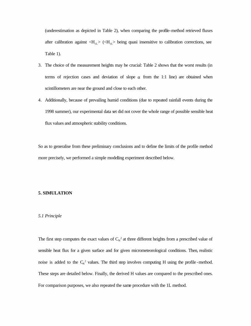
value of the three measurements, <H1L>. This figure gives idea of the consistency of the

scintillometers’ response. The characteristics of the linear regressions Hscint = α <H1L> obtained are

given in Table 1. Despite small systematic differences between the instruments, the agreement is quite

satisfactory. Merging the whole data set, we can consider that the three LAS provide a ±5%

accuracy on the sensible heat flux. This control demonstrates (i) the reliability of the 3 scintillometers’

measurements and (ii) the fact that –as the retrieved sensible heat flux remains constant with height-

the instruments are all placed in the surface boundary layer. The data set therefore appears consistent

and quite suitable for testing the profile method which should provide similar fluxes in these

conditions.

4.2 Profile method

The profile method has been applied in the 3 possible combinations of two levels (2.50 and 3.45 m),

(2.50 and 6.45 m) and (3.45 and 6.45 m). No correction for inter-calibrating the instruments have

been done in a first step. Because of the doubts about the representativity of the 3D sonic

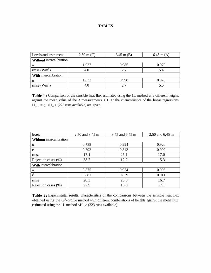
anemometer/eddy correlation measurements, we only present here the comparison against <H1L>

(Fig. 7). In addition to a deviation from the 1:1 line, it shows a considerable increase of the scatter

whatever the couple of heights considered: Table 2 shows that the rms error of the linear regressions

Hprofile = α <H1L> reaches 25 Wm-2 and is much larger than the single level

measurements. Moreover, critical problems appear in some cases (the occurrence of rejections is

also indicated in Table 2): computations either may lead to unrealistic values not even plotted in Fig.

7 (out of scale), or they may simply be impossible, the estimated ratio r (Eq. 9) being out of the

range 1 < r < (z2/z1)2/3 previously defined (see Eq. 10) for unstable conditions.

The failure of the profile method is easy to explain. For near-neutral conditions, f(z/L) tends towards

4.9 (see Eq. 3 and 4) and the ratio r towards 1; the denominator of Eq. 10 then ends towards 0,

making the computation of L subject to very large errors. These propagate on u* through eq. (5),

which may lead to unrealistic values of u*T*. Similarly, under very unstable conditions, r → (z2/z1)2/3

and L → 0 according to equation (10). f(z/L) then tends towards 0 (see Eq. 3), which possibly

induces large errors on the estimate of T* (see Eq. 2) and finally on H.

As it determines that of r, the accuracy of CN2 measurements is therefore likely to limit the accuracy

of estimates of H under atmospheric conditions (near neutral and highly unstable) in which H is over-

sensitive to r. Computations may even be simply impossible when measurement errors on the

structure parameters CN12 and CN2

2 at both heights or a poor inter-calibration of the instruments

make the inequalities r > 1 (near neutrality) or r < (z2/z1)2/3 (very unstable) to be not satisfied.

This is consistent with the results of other authors who have commented on the sensitivity of the

profile method to the inter-calibration and accuracy of the scintillometers. Andreas (1988) already

noted the uncertainties of the CT2-profile method for near-neutral conditions and under highly

unstable conditions. Hill et al. (1992) compared scintillometer derived sensible heat flux H and

friction velocity u* using the CT2-profile method against eddy correlation measurements on a small

dataset: they attributed to systematic differences between their scintillometers the rather poor

agreement they observed for H and the systematic deviation for u*.

Following recommendations given by Hill et al. (1992), we also tested the results obtained with inter-

calibrated data (1L and profile methods). For this, we used ‘inter-calibrated’ CN2 values retrieved

from the regressions indicated in Fig. 2. The results are presented in Tables 1 and 2. No significant

improvement appears when comparing with the previous results obtained with raw (i.e. non

calibrated) CN2 values.

At this point of the study one may conclude from the experimental results that:

1. Provided z0 is known, the 1L method is much more robust than the profile method. The profile

method is very sensitive to measurement errors, particularly in near-neutral and very unstable

conditions.

2. The possible improvement brought by a careful inter-calibration of the scintillometers before

using the profile method, as recommended by several authors, could not be fully addressed with

our data set. The reasons lie in the poor confidence we have in our intercalibration experiment.

First the experiment was too short (only 1 day). Secondly it suffered from the lack of a credible

independent reference measurement of CN2. This probably translates into a remaining bias

(underestimation as depicted in Table 2), when comparing the profile-method retrieved fluxes

after calibration against <H1L> (<H1L> being quasi insensitive to calibration corrections, see

Table 1).

3. The choice of the measurement heights may be crucial: Table 2 shows that the worst results (in

terms of rejection cases and deviation of slope α from the 1:1 line) are obtained when

scintillometers are near the ground and close to each other.

4. Additionally, because of prevailing humid conditions (due to repeated rainfall events during the

1998 summer), our experimental data set did not cover the whole range of possible sensible heat

flux values and atmospheric stability conditions.

So as to generalise from these preliminary conclusions and to define the limits of the profile method

more precisely, we performed a simple modelling experiment described below.

5. SIMULATION

5.1 Principle

The first step computes the exact values of CN2 at three different heights from a prescribed value of

sensible heat flux for a given surface and for given micrometeorological conditions. Then, realistic

noise is added to the CN2 values. The third step involves computing H using the profile -method.

These steps are detailed below. Finally, the derived H values are compared to the prescribed ones.

For comparison purposes, we also repeated the same procedure with the 1L method.

For a surface characterised by its roughness length and displacement height (prescribed values),

simulation runs were performed over a large range of H and of atmospheric stability conditions

(though we only focus on unstable conditions in this paper). The data required were wind speed at a

given reference height, air temperature and net radiation. Practically a run is performed as follows :

1. u* is first calculated using an iterative procedure combining Eq. (6) and an expression of Monin-

Obukhov length. L is corrected for humidity following Panofsky and Dutton (1984) as :

( )β

ρ

0.07/ 1 H gk

u TL

3

*a

+−=

pc (12)

The Bowen ratio is estimated as β = H/(Rn-H-G) where the ground heat flux G is here taken as

G = 0.15 Rn.

T* is then computed as T* = H/ρ cp u* . C T2 can then be estimated from Eq. (2) and (3). Finally

CN2 is computed using Eq. (1).

2. Realistic errors (in terms of magnitude and statistical distribution) are then assigned to CN2.

• In what follows we first examine the sensitivity to instrumental errors only. For this purpose the

exact CNi2 values at level i (i = 1, 2 or 3 for the 3 scintillometers) are replaced by

CNi2 (1 + 0.01δi). The relative errors δi (expressed in percent) for each instrument are randomly

selected for every run from 3 normal distributions having the same prescribed standard deviation

(σ). The 3 errors are therefore independent from each other.

• A second step evaluates the sensitivity to calibration errors only. The instrumental errors are now

set to 0, and every CNi2 (i = 1, 2, 3) value is modified by a systematic error, i.e. replaced by

(1 + ε i) CNi2, εi depending on the instrument (i.e. the measurement height) only, and being kept

constant for all the runs.

3. H is finally computed again applying the profile-method as described in section 2.3

All the simulations have been made with a constant net radiation of 550 Wm-2 and air temperature of

30°C. Reference height is 4 m. In order to have a range of z/L values as large as possible, the

sensible heat flux H and wind speed u are given random values (with a uniform distribution) and

allowed to vary respectively between 0 and 450 Wm-2 and between 0.5 and 5.5 ms -1. 4000 runs are

repeated for each simulation. Before performing the sensitivity study, we first checked the code by

assigning a 0 value to CN2 errors and verifying the H flux initially prescribed was correctly retrieved.

5.2 Sensitivity to instrumental errors

5.2.1 Simulation of Zapata data

We used the scintillometer heights (i.e. 2.50, 3.45 and 6.45 m) and surface characteristics (i.e.

z0 = 10 cm and d = 30 cm) encountered on the Zapata site. We assumed that the instruments were

perfectly inter-calibrated and that measurements were only affected by instrumental errors δi (i = 1, 2,

3). Four simulations have been performed assuming standard deviations (σ) of instrumental errors of

2.0 %, 3.0 %, 4.0 % and 5.0 % successively, the latter corresponding to the order of magnitude

found after the inter-comparison experiment (see section 3.2).

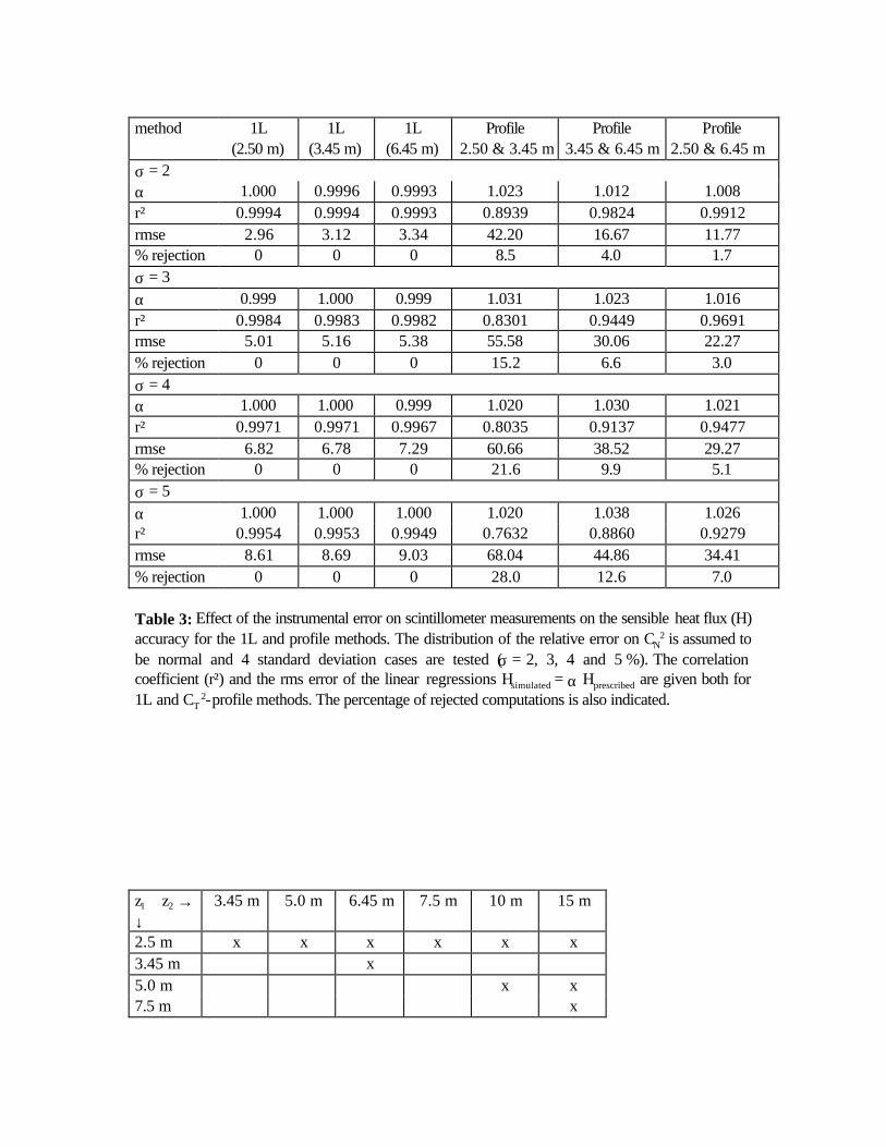
Table 3 shows the statistics for the regression between simulated -by both 1L and profile methods-

and prescribed H values, Hsimulated = α Hprescribed, forced through the origin. Table 3 also gives the

percentage of rejection cases (impossible computations or unrealistic results). Fig. 8a and 8b

illustrate results for σ = 5 %. The scatter remains very large whatever the combination of heights

considered: the rms error characterises the standard deviation of the error on simulated H values and

varies between 34 Wm-2 (for 2.50 and 6.45 m combined heights) to 68 Wm-2 (for 2.50 and 3.45

m). To give an idea, if we assume the error in H follows a normal distribution, a rmse of 30 Wm-2

(which means that 99% of the points are within a ±90 Wm-2 interval) roughly corresponds to a ±30%

relative accuracy on H (whose average prescribed value is around 300 Wm-2).

For comparison, Fig. 8c shows that the sensitivity of the classical 1L method to instrumental errors is

much more limited, the simulated H not differing from its prescribed value by more than ±6%. Table

3 shows that, whatever the instrumental error σ, the accuracy of the 1L method is at least four times

better than the profile method. It also appears that the accuracy of the profile method is reduced

significantly when the two heights of measurement are close to each other and/or close to the ground.

The simulations confirm that the instrumental errors can be responsible for the impossibility of

performing retrievals in a number of cases (up to 28 %, see Table 3). These impossibilities are

encountered near neutrality, or for high atmospheric unstability, for which computations must be

rejected. This may limit the usefulness of the profile method for practical applications, for instance

when a continuous monitoring of sensible heat flux is expected.

After having confirmed by these simulations the sensitivity to instrumental errors, as observed in our

experimental results (see section 4.2), the question now rises if a suitable choice of the measurement

heights would yield a better performance from the CT ²-profile method.

5.2.2 Effect of height of the instruments

Andreas (1988) showed that the larger the ratio of measurement heights, the more accurate the

determination of z/L by the profile-method. He also discussed the practical constraints imposed by

the location of the instruments, not too close to the surface for the lower one, and inside the surface

boundary layer for the upper one.

We performed simulations to test the sensitivity of the profile-method to the heights of instruments.

All the configurations tested are indicated in Table 4. They allowed us to test the sensitivity of z2/z1

ratios ranging between 1.38 and 6. The lower level z1 must be chosen with a particular care. As a

matter of fact, in the framework of similar previous experiments over grass (not yet published), the

comparison between sensible heat fluxes estimated by the classical 1L method at 2 heights revealed

systematic underestimation of H for too small z1 (lower than 2 m). Hill et al. (1992) mention the

same problem with a scintillometer placed at 1.45 m. Moreover, for long propagation paths, LAS

measurements are more prone to saturation if performed close to the ground. The saturation distance

depends on the characteristics of LAS: for instance, according to Hartogensis (1997) who used the

same instrument as ours, H fluxes up to 500 Wm-2 can be measured only on distances under 500 m

at 1 m height and under 700 m at 2 m. For these reasons, we performed our simulations with

z1 = 2.5 m. The other constraint imposed by the surface boundary layer height for the choice of

z2 also contributes to limit the ratio z2/z1 for practical applications.

As the CT2 profile shape -and consequently the CT

2 ratio at two given heights- obviously depends on

the aerodynamic characteristics of the surface, we tested 2 cases : (i) z0 = 10 cm and d = 30 cm (as

in the Zapata site), and (ii) z0 = 2 cm and d = 0 cm (which typically corresponds to short grass).

Finally computations were done for three values of the standard deviation of the instrumental error,

σ = 2, σ = 3 and σ = 5 %.

We only present here synthetic results illustrating the impact on 2 variables : the rms error for H and

the percentage of rejection cases.

Fig. 9a shows the variation of the rms error (rmse) on H against the z2/z1 ratio, the lower height z1

being kept constant (z1 = 2.5 m). The rmse first rapidly decreases with z2/z1 and it remains rather

constant for z2/z1 ratios greater than 4. The rmse is obviously larger for important instrumental noise,

whatever the aerodynamic characteristics of the surface, as it can easily be seen in Fig. 9a. High

values of z2/z1 (∼ 6) tend to reduce the sensitivity of the instrumental error on H, but are not easily

compatible with the practical constraints discussed above. We also note that for a given combination

of heights, the CT2-profile method is more robust above low vegetation cover. For a given height

ratio (z2/z1 = 2, Fig. 9b) one can see the best accuracy on H is obtained for the highest possible

levels. The percentage of rejection cases rapidly decreases with z2/z1 for z1 = 2.5 m (Fig. 10a). But

for the given ratio z2/z1 = 2, it behaves differently from the rmse and increases with z1 (Fig. 10b). For

a given location of instruments, the percentage of rejection is very sensitive to the instrumental error

and to the roughness of the surface.

Simulations finally show that the best trade off is achieved by choosing z2/z1 ∼ 3 or 4 with z1 ∼ 2 or

2.5 m. It is compatible with the practical constraints encountered for locating the instruments, i.e.: (i)

the highest level remains below the top of the surface boundary-layer and, (ii) the lowest level is

above a minimum height from the surface so as to avoid underestimated measurements of CN2. In

these conditions, the greatest accuracy attainable for H would be about ±10% (rmse ∼10 Wm-2)

obtained with a hypothetical instrument having a precision characterised by a σ = 2% normal

distribution of the relative error. This is to be compared to an accuracy for H of about ±30% (rms

∼25 Wm-2) obtained with a more realistic instrument having a lower relative accuracy (σ = 5 %). For

the same ratio of heights, Fig. 10a shows that the percentage of rejection cases varies between 2 and

12% depending on the type of surface and the accuracy of scintillometers (instrumental error). A

rapid degradation of these performances occurs when the height of scintillometers is altered.

5.3 Sensitivity to calibration errors

The instrumental error has been here set to 0, and only a calibration error has been simulated. For

this purpose, systematic deviations ε i (i = 1, 2, 3) from the exact CN2 value were introduced on each

instrument response. We did not peformed a systematic study of the effect of instruments’

miscalibration, but limited us to a few examples based on the case studies depicted in Table 5 to

illustrate the possible errors for H. The sensitivity tests have been made using measurement heights of

2.5, 5.0, and 10.0 m, with z0 = 10 cm and d = 30 cm for the characteristics of the surface. We only

considered the combinations of levels including the lowest height z1 = 2.5 m, ie (2.5 and 5.0 m) and

(2.5 and 10.0 m). For clarity, we only present here cases for which instruments deviate

symmetrically from the 1:1 line with opposite signs. But we controlled that the results were quite

similar if only one of the instruments was affected by an equivalent overall error: for instance cases (-

2 %, +2 %) and (0 %, + 4 %) or (-4 %, 0 %) provided the same results. At least for small

calibration errors, which seems to be important is the difference of calibration of both instruments.

We evaluated the consequences of differences in calibration of up to ±4 % (cases 3 and 4) between

instruments.

Fig. 11 displays the comparison between simulated and prescribed H values obtained when

combining the two lower levels (2.5 and 5.0 m) and simulating a +4 % and –4 % calibration

difference successively between instruments. The two cases 3 and 4 (see Table 5) are gathered in

Fig. 11: combined calibration errors of –2 % and +2 % for the lower and upper instrument

respectively induce a systematic overestimation of H (see circles); on the opposite, triangles in the

same figure correspond to a simulation performed with calibrations errors of +2 % and –2 % (at

lower and upper levels of measurement). Despite this being a worst scenario (even though Nieveen

and Green (1999) found a 5 % deviation on one of their instruments), it is given to introduce the

criteria used in next figure: the scatter for H and its systematic deviation from the 1:1 line can simply

be characterized by considering the two relative deviations d1 and d2 from the 1:1 line at an arbitrary

H value (we took H ∼ 300 Wm-2, see Figure 11). d1 and d2 provide a helpful, despite qualitative,

criteria to evaluate different configurations of calibration errors in what follows.

A synthesis of the results is presented in Fig. 12. The calibration difference between the two

considered instruments (‘high’ minus ‘low’) is plotted along the X-axis. The Y-axis represents the

relative error on the retrieved H values (for H ∼ 300 Wm-2) which ranges between the extreme

values d1 and d2 previously defined. d1 and d2 increase (in absolute value) with the difference of

calibration between the instruments. This defines an area (grey tones in Fig. 12) containing the

possible values of the error for H. As an example, we see in Fig. 12 that for 2 instruments placed at

2.5 and 5 m and having a 3 % difference in calibration, the error is likely to situate between –3 and –

9 % or between +3 and +15 % depending on the fact either the upper or lower instrument is over-

calibrated. Fig. 12 shows three such ‘error areas’ corresponding to the CT2-profile method applied

to heights of (i) 2.5 and 5.0 m, (ii) 2.5 and 10.0 m, and (iii) to the classical 1L method (given here for

comparison purposes).

It appears that the lowest levels (2.5 and 5.0 m) tend to cause the largest errors on H. The sensitivity

of the profile method to measurements errors when both instruments are placed too near from the

surface is confirmed, as it had already been pointed out for the instrumental error (see 5.2). When

the calibration of both instruments is satisfactorily (say within ±1%), the resulting error on H is much

smaller than the one induced by instrumental error. This confirms the small influence we noted on our

experimental results when introducing a calibration correction. Choosing a larger z2/z1 ratio (levels

2.5 and 10 m) reduces the sensitivity to calibration error to a few percent, as indicated by the dotted

lines in Fig. 12. The 1L method is the most robust, the resulting error on H being of the same order

of magnitude as the calibration error with no amplification effect (see thin continuous lines in fig. 12).

6. DISCUSSION

An experiment combining measurements of scintillations with large aperture scintillometers placed at

three heights (2.50, 3.45 and 6.45 m) over natural grassland (330 m propagation path) in Mexico

was designed to test the potential of CT2-profile method for estimating sensible heat flux H. The

classical method (1L) which consists in measuring scintillations at a single level but which requires an

independent estimation of u* has also been used for comparison purposes. The results confirm the

robustness of the 1L method, provided the roughness length is correctly estimated. The comparison

between the CT2-profile method derived H against the average of the 1L method estimations (taken

as a reference) shows considerable scatter, particularly when the two levels used are close to each

other and/or close to the surface. The rms error is about 5 Wm-2 for the 1L method, compared with

the 17 to 25 Wm-2 rmse range obtained with the profile method (depending on the combinations of

levels used). The experiment reveals significant limitations of the profile method: namely unrealistic

estimations of H and the impossibility of performing the computations in either near-neutral conditions

or very unstable conditions. These limitations are easily explained by the sensitivity of the equations

used to measurement errors through the ratio between CT2 at two heights. Numerical simulations

confirm these results.

Two types of measurement error on CN2 are identified. The ‘calibration error’ corresponds to a

systematic deviation of the scintillometer response from the actual values of CN2. What we refer to as

the ‘instrumental error’ corresponds to the scatter around a calibration curve. We assumed this to be

random noise (gaussian distribution). The inter-calibration experiment performed did not allow us to

characterise precisely these two errors. For future experiments, we recommend a careful inter-

calibration procedure.

The numerical experiments consisted of simulating actual CN2 data by adding a noise to exact CN

2

values computed from prescribed H over a given surface, and then retrieving H by both the classical

1L and CT2-profile methods. Comparison between computed and prescribed H values allowed an

evaluation of both methods. For instrumental error (expressed in terms of relative error) we tested

the effect of gaussian distributions of noise with standard deviation ranging between 2 % and 5 %.

For the calibration error we examined the effect of differences between instruments up to ±4 %.

The simulations confirmed the experimental results: the sensitivity of the CT2-profile method to

measurement errors is likely to explain the large scatter we observed on Mexico data set. The

sensitivity to instrumental errors appears so large in many cases that, even with a good inter-

calibration of the scintillometers, the CT2-profile method remains prone to large errors. The

simulations showed that the closer to the ground or to each other are the instruments, the higher is the

sensitivity to instrumental errors. It also shows that the profile method is much more sensitive to

measurement errors than the 1L method. For both calibration and instrumental errors, the simulations

indicated that the larger the difference between measurement heights is, the better the estimations of

H are. This condition is not always easy to fulfil: the upper level must be in the surface boundary

layer, while the lower one must not be too close to the surface. A combination of measurement

heights around 2.5 and 10 m generally provides a good trade off for vegetation heights of 50 cm or

less. The characteristics of the surface also play a role, and we have shown that results were better

for a vegetation with low roughness and displacement height.

Let us insist on the fact that, in this paper, we only tested the sensitivity of the 1L and CT2-profile

methods to CN2 measurement errors. The profile method is ‘self-sufficient’ to estimate H whilst the

1L method requires to know the roughness length, which introduces another source of error, not

taken into account in this paper. A rule of thumb estimation of z0 is realistic for a dense homogeneous

vegetation and allows a robust estimation of H (McAneney et al., 1995). This might not be the case

for heterogeneous vegetation or composite surfaces for which the definition of an ‘equivalent

roughness’ still remains unclear and poses problems of aggregation; the consequence of z0 errors on

the final accuracy for H should be evaluated in these cases. Despite this, the over-sensivity of the

profile method to CN2 errors is likely to make it less competitive than the 1L method for estimating H.

Another limitation of the CT2-profile method lies in a number of cases for which computations are

impossible or results unrealistic. They occur for near-neutral or very unstable conditions. The number

of ‘rejection’ cases depends on the location of instruments and on the aerodynamic characteristics of

the surface, but may reach as much as 30% according to the experimental results and to the

simulations. This may drastically limit the practical interest of the profile method when a continuous

monitoring of fluxes is desired.

Acknowledgements

The authors are indebted to CNES (Centre National d'Etudes Spatiales)/(Terre Ocean Atmosphere

Biosphere) TAOB and IRD (Institut de Recherche en Développement) who funded this study, and

to the IRD/IMADES (Instituto del Medio Ambiente y el Desarrollo Sustentable del Estado de

Sonora) who supported the field experiment.

Part of this study has been carried out in the context of a joint research project on scintillometry with

the Department of Meteorology of the Wageningen University, who also provided the instruments.

REFERENCES

Andreas E.L., 1988 : Atmospheric stability from scintillation measurements. Applied optics, Vol. 27,

No. 11, 2241-2246.

Avissar R., 1991 : A statistical-dynamical approach to parameterize subgrid-scale land-surface

heterogeneity in climate models. Surv. Geophys., 12, 155-178.

Brunet Y., 1996 : La représentation des paysages et la modélisation dans le domaine de l’environnement.

In : Tendances nouvelles en modélisation, pour l’environnement. Elsevier, Paris, 59-77.

Chehbouni A., Njoku E.G., Lhomme J.P., Kerr Y.H., 1995 : Approaches for averaging surface

parameters and fluxes over heterogeneous terrain. J. Climate, 8, 1386-1393.

De Bruin H.A.R., Van den Hurk B.J.J.M., Kohsiek W., 1995 : The scintillation method tested

over a dry vineyard area. Boundary-Layer Meteorol., 76, 25-40.

Goodrich D.C. and 30 co-authors, 1998 : An overview of the 1998 activities of the semi-arid Land-

Surface Program. In : Proc. of the 1998 American Meteorological Society meeting. Phoenix, AZ, 1-7.

Green, A.E., McAneney, K.J., Astill, M.S., 1994 : Surface layer scintillation measurements of

daytime heat and momentum fluxes. Boundary-Layer Meteorol., 68 357-373.

Green A.E., McAneney K.J., Lagouarde J.P., 1997 : Sensible heat and momentum flux

measurement with an optical inner scale meter. Agric. For. Meteorol., 85, 259-267.

Hartogensis O., 1997 : Measuring areally-averaged sensible heat fluxes with a Large Aperture

Scintillometer. Report, Department of Meteorology, Agricultural University of Wageningen, The

Netherlands.

Hill R.J., 1992 : Review of optical scintillation methods of measuring the refractive-index spectrum,

inner scale and surface fluxes. Waves in Random Media, 2, 179-201.

Hill R.J., Ochs G.R., Wilson J.J., 1992 : Surface-layer fluxes measured using the CT2-profile

method. J. of Atmospheric and Oceanic Technology, 9, 5, 526-537.

Kaimal J.C., Finnigan J.J., 1994 : Atmospheric boundary layer flows : their structure and

measurement. Oxford University Press.

Lagouarde J.P., McAneney K.J., Green A.E., 1996 : Spatially-averaged measurements of sensible

heat flux using scintillations : first results above a heterogeneous surface. "Scaling-up in Hydrology using

remote sensing" workshop, June 10-12 1996, Institute of Hydrology, Wallingford, G.B., Wiley & sons

Ed., 147-160.

McAneney, K.J., Green, A.E. and Astill, M.S., 1995 : Large-aperture scintillometry: the

homogeneous case. Agric. and Forest Meteorol. , 76, 149-162.

Nieveen J.P., Green A.E., 1999 : Measuring sensible heat flux over pasture using the CT2-profile

method. Boundary-Layer Meteor., in press.

Noilhan J., Lacarrère P., 1995 : GCM grid-scale evaporation from mesoscale modelling. J. Climate, 8,

206-223.

Ochs G.R., Cartwright W.D., 1980 : Optical system model IV for space-averaged wind and CN2

measurements. NOAA Tech. Memor. ERL WPL-52. NOAA Environmental Research Laboratories,

Boulder, CO, USA.

Ochs G.R., Wilson J.J., 1993 : A second-generation large-aperture scintillometer. NOAA technical

Memorandum ERL WPL-232. NOAA Environmental Research Laboratories, Boulder, CO, USA.

Panofsky H.A., Dutton J.A., 1984 : Atmospheric turbulence : models and methods for engineering

applications. John Wiley & Sons, New York.

Raupach M.R., 1995 : Vegetation-atmosphere interaction and surface conductance at leaf, canopy and

regional scales. Agric. For. Meteor., 73, 151-179.

Raupach M.R., Finnigan J.J., 1995 : Scale issues in boundary-layer meteorology : surface energy

balance in heterogeneous terrain. Hydrol. Processes, 9, 589-612.

Wyngaard J.C., 1973 : On surface-layer turbulence. Workshop on Micrometeorology, Denver,

Colorado, Amer . Meteor. Soc., 101-149.

LIST OF CAPTIONS

Fig. 1: (a): Zapata experimental site; the propagation path of the scintillometers is indicated by a

thick segment, and the location of the meteorological and 3D reference measurements by a dot. (b):

location of the scintillometers (A, B, C); the square dot corresponds to the location of the 3D sonic

anemometer and of the micrometeorological station (the list of instruments is given in the text); the

area indicated by the dotted circle corresponds to wetter and higher vegetation (see text).

Fig. 2: Inter-calibration of the three scintillometers. The x-axis represents the average value of the

three measured CN2. The "forced through 0" regressions are also indicated.

Fig. 3: Distribution of the relative measurement error on CN2 observed during the inter-calibration

experiments performed in Audenge (SW France, 1997) and in Zapata (Mexico, 1998). The normal

distributions with standard deviations 4, 5 and 6.0 % are also plotted.

Fig. 4: Histogram of the roughness length values z0 retrieved from 3D sonic anemometer

measurements.

Fig. 5: Comparison of sensible heat flux estimated at Zapata site from the three scintillometers using

the 1L method at every height independently against H measured using a 3D sonic anemometer.

Fig. 6: Comparison of sensible heat flux estimated at Zapata site from the three scintillometers using

the 1L method at every height independently against the mean H values <H 1L>.

Fig. 7: Comparison of the sensible heat flux estimated at Zapata site by the CT²-profile method

against <H 1L> for the three possible combinations of heights.

Fig. 8: Simulation of the sensible heat flux using the CT²-profile method, assuming a relative

instrumental error following a normal distribution with a 5.0 % standard deviation, and for different

combinations of scintillometer heights (a: 2.50 and 6.45 m; b: 2.50 and 3.45 m). For comparison

purposes, the simulation using the 1L method for each scintillometer is given in Fig. 8c.

Fig. 9: Simulation study of the sensitivity of the CT²-profile method to the respective locations of the

scintillometers. (a): rms retrieval error for H vs the ratio z2/z1 (using the same lower height z1 = 2.5

m); (b): rms retrieval error for H as a function of the lower height z1 (for a given height ratio

z2/z1 = 2). Three cases of instrumental errors have been tested (σ = 2 %: triangles, σ = 3 %: squares

and σ = 5 %: circles), as well as two surface types (‘high’ vegetation: full lines, and ‘low’ vegetation:

dotted lines).

Fig. 10: Same as Fig. 9, but for the percentage of rejection cases (CT ²-profile method leading to

impossible computations or unrealistic results).

Fig. 11: Simulation study of the sensitivity of the CT ²-profile method to inter-calibration errors. The

example given here has been done for scintillometers located at 2.50 and 3.45 m; two cases of 4 %

inter-calibration difference between instruments have been tested: circles correspond to combined

calibration errors of –2 % and +2 % for the lower and upper instrument respectively; similarly

triangles correspond to a (+2 %, -2 %) set of calibration errors. The deviations d1 and d2 from the

1:1 line at an arbitrary value H = 300 Wm-2 allow to characterise the scatter (see text).

Fig. 12: Sensitivity of the CT²-profile method to inter-calibration errors: for a given combination of

heights the relative errors on H resulting from inter-calibration differences between the two

instruments (x-axis) are situated in an area between two curves. The thick lines and the dark grey

area correspond to a combination of scintillometers' heights of 2.5 and 5.0 m; the dotted lines

correspond to the combination of heights 2.5 and 10.0 m. For comparison purpose, the thin lines

indicate the sensitivity of the 1L method to inter-calibration errors (clear grey area).

TABLES Levels and instrument 2.50 m (C) 3.45 m (B) 6.45 m (A) Without intercalibration α 1.037 0.985 0.979 rmse (Wm-2) 4.0 2.7 5.4 With intercalibration α 1.032 0.998 0.970 rmse (Wm-2) 4.0 2.7 5.5 Table 1 : Comparison of the sensible heat flux estimated using the 1L method at 3 different heights against the mean value of the 3 measurements <H1L>: the characteristics of the linear regressions Hscint = α <H1L> (223 runs available) are given. levels 2.50 and 3.45 m 3.45 and 6.45 m 2.50 and 6.45 m Without intercalibration α 0.788 0.994 0.920 r2 0.892 0.843 0.909 rmse 17.1 25.1 17.0 Rejection cases (%) 38.7 12.2 15.3 With intercalibration α 0.875 0.934 0.905 r2 0.881 0.839 0.911 rmse 20.3 23.3 16.7 Rejection cases (%) 27.9 19.8 17.1 Table 2 : Experimental results: characteristics of the comparisons between the sensible heat flux obtained using the CT

2-profile method with different combinations of heights against the mean flux estimated using the 1L method <H1L> (223 runs available).

method 1L

(2.50 m) 1L

(3.45 m) 1L

(6.45 m) Profile

2.50 & 3.45 m Profile

3.45 & 6.45 m Profile

2.50 & 6.45 m σ = 2 α 1.000 0.9996 0.9993 1.023 1.012 1.008 r² 0.9994 0.9994 0.9993 0.8939 0.9824 0.9912 rmse 2.96 3.12 3.34 42.20 16.67 11.77 % rejection 0 0 0 8.5 4.0 1.7 σ = 3 α 0.999 1.000 0.999 1.031 1.023 1.016 r² 0.9984 0.9983 0.9982 0.8301 0.9449 0.9691 rmse 5.01 5.16 5.38 55.58 30.06 22.27 % rejection 0 0 0 15.2 6.6 3.0 σ = 4 α 1.000 1.000 0.999 1.020 1.030 1.021 r² 0.9971 0.9971 0.9967 0.8035 0.9137 0.9477 rmse 6.82 6.78 7.29 60.66 38.52 29.27 % rejection 0 0 0 21.6 9.9 5.1 σ = 5 α 1.000 1.000 1.000 1.020 1.038 1.026 r² 0.9954 0.9953 0.9949 0.7632 0.8860 0.9279 rmse 8.61 8.69 9.03 68.04 44.86 34.41 % rejection 0 0 0 28.0 12.6 7.0 Table 3: Effect of the instrumental error on scintillometer measurements on the sensible heat flux (H) accuracy for the 1L and profile methods. The distribution of the relative error on CN

2 is assumed to be normal and 4 standard deviation cases are tested (σ = 2, 3, 4 and 5 %). The correlation coefficient (r²) and the rms error of the linear regressions Hsimulated = α Hprescribed are given both for 1L and CT

2-profile methods. The percentage of rejected computations is also indicated. z1 z2 → ↓

3.45 m 5.0 m 6.45 m 7.5 m 10 m 15 m

2.5 m x x x x x x 3.45 m x 5.0 m x x 7.5 m x

Table 4: Combinations of heights (indicated by symbol x) used to test the sensitivity of the CT2-

profile method to the location of scintillometers.

Deviation (%) case 1 2 3 4 ε3 (z3 = 10.0 m) -1 +1 -2 +2 ε2 (z2 = 5.0 m) -1 +1 -2 +2 ε1 (z1 = 2.5 m) +1 -1 +2 -2 Table 5: Sets of calibration errors (in %) introduced for testing the CT

2-profile method. For each of the four cases, the sensitivity study has been performed for the combination of levels (z1, z2) and (z1, z3).