Page 1
1
Analysis of the regional impacts of Climate Policy in Japan
Shigeharu Okajima
Department of Agricultural, Environmental and Development Economics
The Ohio State University
[email protected]
Selected Paper prepared for presentation at the Agricultural & Applied Economics
Association’s 2009 AAEA & ACCI Joint Annual Meeting, Milwaukee, WI, July 26-28, 2009.
Copyright 2009 by Shigeharu Okajima. All rights reserved. Readers may make verbatim copies of
this document for non-commercial purposes by any means, provided this copyright notice appears on
all such copies.
Page 2
2
Abstract
After great improvements in energy efficiency in the 1970’s, Japan has made little progress in reducing
energy consumption since 1990, the base year for the Kyoto Protocol. This study is motivated by the recent
growing demands among policy makers to find all possibilities for saving energy. To make informed
decisions on how to save energy, policy makers need detailed information on energy consumption structures
within each jurisdiction.
First, in this article, I decompose national level energy intensity into efficiency and activity effects with
the Fisher Ideal index, and then estimate regressions on prefecture level residential electricity demand between
1990 and 2003. It is found that national level energy intensity declined by seventy three percent from 1970 to
2003; sixty three percent of the decline may be attributed to improvement in energy efficiency. Energy
intensity, however, has slightly increased since early 1990’s.
Secondly, this paper explores the impact of reduction of carbon emission on the economy. I find that the
Japanese government needs to enact the environmental taxes on a $12/ton in order to meet the Kyoto Protocol.
It is also found that imposing a $12/ton environmental tax reduces Japanese GDP by around six percent and
equivalent variations in urban regions fall while equivalent variations in rural regions rise.
Keywords: Fisher index; Energy intensity; Regional Computable General Equilibrium; Environmental taxes
Page 3
3
Ⅰ. INTRODUCTION
After the Kyoto Protocol, many countries agreed to reduce carbon emissions to slow
global warming. Japan, for example, has to reduce carbon emissions by six percent compared to
1990 emissions levels and the government started trying to find ways to meet the obligation. It
seems, however, that there are many different factors that influence the carbon emitted in each
region and that the central government does not always recognize them. For instance, Hokkaido,
the northernmost prefecture in Japan, has a lot of snow. As a result, people living there may use
more electricity during winter than those who are in warmer regions. Another example is
population density. If population density has a positive effect on decreasing energy consumption,
the energy consumption per capita in Tokyo, which is the most populated prefecture in Japan,
may be smaller than that of a less densely populated area. Also, some prefectures have a lot of
heavy industries so they may consume more energy than those with fewer such industries. When
energy consumption structures differ between regions, energy saving measures need to vary by
region based on the differences. Thus, the central government either needs to fully understand
regional differences in energy consumption patterns in order to make informed decisions on how
to save energy, or it should allow each local government to take leadership in reducing energy
consumption within its area of jurisdiction. This paper investigates the impacts of the regional
level policies to limit Japanese carbon dioxide emissions.
Okajima (2008) decomposes energy intensity into efficiency and activity effects using the
Fisher Ideal index in order to determine which prefectures have been most effective in improving
their energy efficiency since 1990 in Japan. When energy intensity declines, there are two
possible reasons for the decline. First, energy efficient technologies or energy saving measures
are adopted and thus less energy is used to produce the same amount of GDP. Second, structural
Page 4
4
changes happen and the number of energy intensive industries decreases, while the number of
less energy intensive industries, such as the service industry, grows. These changes, i.e.
improvements in energy efficiency and structural changes, are essentially different. The former
is called energy efficiency and the latter is called economic activity. By distinguishing energy
efficiency from economic activity, we can tell how much of the decline in energy intensity is due
to the pure efforts to save energy.
In this paper, we discuss two policy issues. First, I examine how regional welfare will
change if the Japanese government imposes environmental taxes to reduce Japan’s aggregated
carbon emissions. From Okajima (2008), it is found that some prefectures have been more
effective in improving their energy efficiency compared to other prefectures. Also, each
prefecture has different geographic features and climate conditions which affect energy
consumption. The study implies that each region has different preference for energy
consumption. Thus, I use different utility functions for each region to analyze the impact of
environmental taxes at the regional level. There is a stream of policy literature that studies
regional taxes. One complication of changing tax rates among regions is the “leakage” effect,
which is also known as “pollution haven” effect. When tax rates are different among regions,
inter-regional firms can reduce production in regions with higher taxes, and instead, increase
activities in the other regions to compensate the decrease. Therefore, this paper assumes that
policy makers impose the same tax rate on all regions and investigates equivalent variation of
each region in order to estimate the effectiveness of environmental taxes more accurately.
Another policy issue studied in this paper is the “rebound” effect. In general, rebound
effect means that a policy exhibits such effects that are totally opposite to policy makers’ original
intention. For example, poorly planned environmental policies could induce more energy
Page 5
5
consumption. Many studies emphasize that emission taxes generate revenues that can be used
for finance cut in existing distorted taxes, which in turn avoids some of the deadweight costs
associated with distorted taxes. However, these policies may encourage people to consume
more goods than before. In this paper, we assume that the production taxes are distorted. The
central government will evenly redistribute revenue from the production taxes to each region.
The reduction of finances by the production tax cut is then covered by the environmental tax.
We estimate how the policy affects the level of carbon emissions.
A CGE model is proposed to analyze environmental taxes and the rebound effect.
According to Partridge and Rickman (1998), CGE models are a powerful tool to analyze inter-
regional climate policies. CGE models allow us to simulate the effects of economic policies and
to analyze the aggregate welfare and distributional impacts of policies. For example, Li and
Rose (1995) examine the effect of an emission limit on a single state, modeled as a small open
economy. Balistreri and Rutherford (2004) and Ross et al. (2004) perfom similar analysis using
models which resolve one state but aggregates the remainder of the economy into five census
regions. Sue Wing (2007) is the first to simultaneously resolve all U.S. states, and to simulate
both the interstate system of taxes and transfers as well as general equilibrium effects of
abatement on the distribution of income.
This paper is unique in that it constructs a computable general equilibrium model which
divides the Japanese economy into eight industries and eight regions, and simulates the effects of
environmental policies in order to investigate the potential impact on Japanese economy.
Although the details of regional differences are important for both local and the central
government decision making, there has been no study investigating energy consumption or
demand structure within Japanese prefectures. A major reason for a lack of regional studies is
Page 6
6
that little reliable data on regional energy consumption has been available in Japan. Scarce as it
still is, prefecture level data is becoming more readily available. We use the data on energy
consumption in Japanese prefectures in the period of 1990 to 2003 which was released by the
Research Institute of Economy, Trade and Industry in 2006.
The remaining sections of the paper are organized as follows: the second section presents
Japan’s energy consumption trend; the third section describes the decomposition and analyses of
energy intensity at the national and prefecture level using a decomposition method; the forth
section presents the structure of the CGE model and the simulation results; and the fifth section
provides concluding remarks.
Ⅱ. JAPANESE ENERGY CONSUMPTION TREND
As a first step, I examine Japan’s energy consumption trend in the last few decades. The
reason why energy consumption trend is analyzed, instead of carbon emissions, is that there is
not enough data about carbon emissions in the past 40 years at regional levels. However, energy
consumption correlates closely to carbon emissions. Therefore, it is reasonable to examine the
trend of Japanese energy consumption, instead of Japanese carbon emissions. Overall, Japan has
become very energy efficient since the 1970’s, but progress is not uniform between sectors.
Industry reduced energy consumption dramatically, while the transportation, commercial, and
residential sector increased energy consumption continuously. In this section, I first outline
Japan’s energy consumption trend. Then I present the energy issues that the Japanese
government now confronts.
Page 7
7
A. Japan’s Energy Consumption Trend
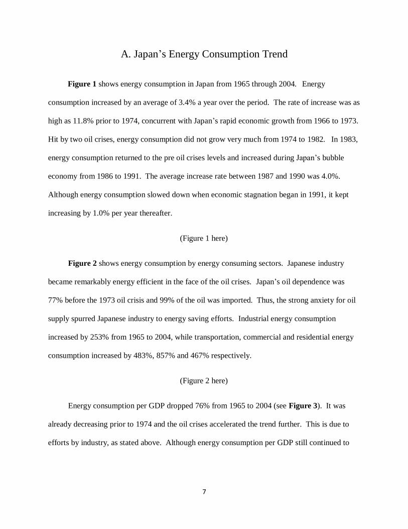
Figure 1 shows energy consumption in Japan from 1965 through 2004. Energy
consumption increased by an average of 3.4% a year over the period. The rate of increase was as
high as 11.8% prior to 1974, concurrent with Japan’s rapid economic growth from 1966 to 1973.
Hit by two oil crises, energy consumption did not grow very much from 1974 to 1982. In 1983,
energy consumption returned to the pre oil crises levels and increased during Japan’s bubble
economy from 1986 to 1991. The average increase rate between 1987 and 1990 was 4.0%.
Although energy consumption slowed down when economic stagnation began in 1991, it kept
increasing by 1.0% per year thereafter.
(Figure 1 here)
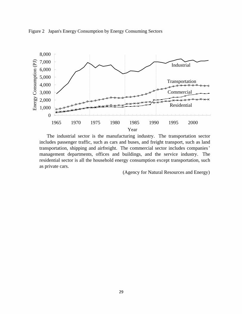
Figure 2 shows energy consumption by energy consuming sectors. Japanese industry
became remarkably energy efficient in the face of the oil crises. Japan’s oil dependence was
77% before the 1973 oil crisis and 99% of the oil was imported. Thus, the strong anxiety for oil
supply spurred Japanese industry to energy saving efforts. Industrial energy consumption
increased by 253% from 1965 to 2004, while transportation, commercial and residential energy
consumption increased by 483%, 857% and 467% respectively.
(Figure 2 here)
Energy consumption per GDP dropped 76% from 1965 to 2004 (see Figure 3). It was
already decreasing prior to 1974 and the oil crises accelerated the trend further. This is due to
efforts by industry, as stated above. Although energy consumption per GDP still continued to
Page 8
8
decline at a slower pace during the bubble economy, it slightly increased when Japan entered
economic stagnation and both energy consumption per capita and GDP per capita leveled off.
(Figure 3 here)
B. Japan’s Energy Issues
After the great improvements made in the 1970’s, Japanese energy saving efforts seem to
have reached a ceiling. Energy consumption per GDP has been gently increasing since 1990 but
had been declining before the 1980’s. Even though the pace has slowed down since 1990,
energy consumption has been rising as well. Japan has to reduce greenhouse gas emissions by
six percent below the 1990 level by 2008 to 2012 to meet the obligations of the Kyoto Protocol.
This is a great challenge as Japan’s energy efficiency improved greatly before 1990 and has been
deteriorating ever since. In reality, energy consumption grew by 115% from 1990 to 2004.
Observing the energy consumption trends, I have found that Japanese industry has become
very energy efficient. Taking into account the fact that manufacturing companies have relocated
their plants overseas since the early 1990’s with only their offices remaining in Japan, as well as
their tireless efforts in past decades, there is little room for improvement in the industrial sector.
On the other hand, energy consumption in the transportation, commercial and residential
sector has been growing rapidly. In 1965 energy consumption in these three sectors represented
36 % of aggregate energy consumption. However, the percentage went up to 55% in 2004.
Therefore, it is especially important to improve energy use in the transportation, commercial, and
residential sector in order to reduce Japan’s aggregate energy consumption. With these issues in
mind, I examine the factors which affect energy intensity in the next section.
Page 9
9
Ⅲ. DECOMPOSITION OF ENERGY INTENSITY
In this section, I analyze energy intensity trends. Energy intensity is the ratio of energy
use to activity, and is usually obtained by dividing GDP into energy consumption. Unlike
energy consumption per capita, energy intensity can tell how efficiently energy is used and can
be used to compare different levels of energy use. As energy consumption is essential to
economic activities, simply capping energy use may deteriorate the economy. Instead, energy
intensity should be used to evaluate energy saving efforts. In the following section, I decompose
an energy intensity index into an efficiency and activity index. First, I explain the decomposition
method with the Fisher Ideal index. Then, I apply the method to national and prefecture level
energy consumption in Japan. Again, the reason why energy consumption trend is analyzed,
instead of carbon emissions, is that there is not enough date about carbon emissions in the past
40 years at regional levels. However, energy consumption correlates closely to carbon emissions.
Therefore, it is reasonable to examine the trend of Japanese energy consumption, instead of
Japanese carbon emissions.
A. Decomposition Method of Energy Intensity
When energy intensity declines, there are two possible reasons for the decline. First,
energy efficient technologies or energy saving measures are adopted and thus less energy is used
to produce the same amount of GDP. Second, structural changes happen and the number of
energy intensive industries decreases, while the number of less energy intensive industries, such
as the service industry, grows. These changes, i.e. improvements in energy efficiency and
structural changes, are essentially different. The former is called energy efficiency and the latter
Page 10
10
is called economic activity. By distinguishing energy efficiency from economic activity, we can
tell how much of the decline in energy intensity is due to the pure efforts to save energy.
Over the past few decades, a considerable number of studies have been conducted on
index numbers that are used to decompose aggregate energy intensity into component elements
of energy efficiency and economic activity. Boyd et al. (1987) introduced the Divisia index
approach and Tornqvist approximation. These decompositions, however, had a residual term. If
there are residual terms, they may have effects on an energy intensity index and we may
misinterpret results. Therefore, we have to think about another index approach that has no
residual term. Fisher (1921) indicated that Fisher Ideal indices can completely decompose an
expenditure index into a price and quantity index. Applying this idea, Boyd and Roop (2004)
showed that the Fisher ideal index provides a perfect decomposition of an aggregate energy
intensity index into an economic activity and an energy efficiency index with no residual.
However we cannot always accomplish this decomposition. According to Diewert (2001), we
can achieve this decomposition if the following conditions are met: we can construct sectors that
account for all energy use in the economy without overlap; and, there exists a set of economic
activity measures itY with which to construct a measure of energy intensity.
Aggregate energy intensity ( te ) is a function of sectoral energy efficiency ( ite ) and
sectoral activity ( ita ).
itit
t
it
i it
it
t
t
t aeY
Y
Y
E
Y
Ee
(1)
where tE is aggregate energy consumption in year t, itE is energy consumption in sector i in
year t, tY is GDP in year t, and itY is a measure of economic activity in sector i in year t. The
Page 11
11
sum total of energy consumption in sectors must be equal to aggregate energy consumption,
whereas the sum total of measures of economic activity needs not equal to GDP.
I first construct the Laspeyres and Paasche index and an efficiency and activity index in
order to construct the Fisher Ideal index. In terms of energy intensity, the Laspeyres approach
uses a base year fixed weight for energy consumption and economic activity measures. The
Laspeyres index is
i
ii
i
iti
act
tae
ae
L00
0
(2)
i
ii
i
iit
eff
tae
ae
L00
0
(3)
where act
tL is the Laspeyres activity index and eff
tL is the Laspeyres efficiency index. By
reversing the role of the base year (t=0) and the end year (t=T), we can construct the Paasche
index. Therefore the Paasche index is
i
iit
i
itit
act
tae
ae
P0
(4)
i
iti
i
itit
eff
tae
ae
P0
(5)
Page 12
12
where act
tP is the Paasche activity index and eff
tP is the Paasche efficiency index. The Fisher
Ideal index is the geometric average of the Laspeyres and Paasche index. The Fisher Ideal index
is
act
t
act
t
act
t PLF (6)
eff
t
eff
t
eff
t PLF (7)
According to Boyd and Roop (2004), the Fisher Ideal index satisfies the property
equivalent to perfect decomposition. The property, factor reversal, means that an acceptable
functional form of the price index TT qqppp ,0,,0 should be acceptable to the quantity index
TT qqppQ ,0,,0 as well with the roles of the price and quantity vector reversed and that the
quantity index must satisfy 0V
VT TT ppqqP ,0,,0 TT qqppQ ,0,,0. Thus, the Fisher Ideal index
allows us to segment an aggregate energy intensity index into an efficiency and activity index
with no residual. Denoting 0e as aggregate energy intensity for a base year, an energy intensity
index ( tI ) can be constructed. The decomposition of an energy intensity index into an activity
and efficiency index is
eff
t
act
ttt FFI
e
e
0
(8)
Applying this decomposition method, we can determine how energy intensity would have
changed if either an efficiency or activity index had not changed at all.
Page 13
13
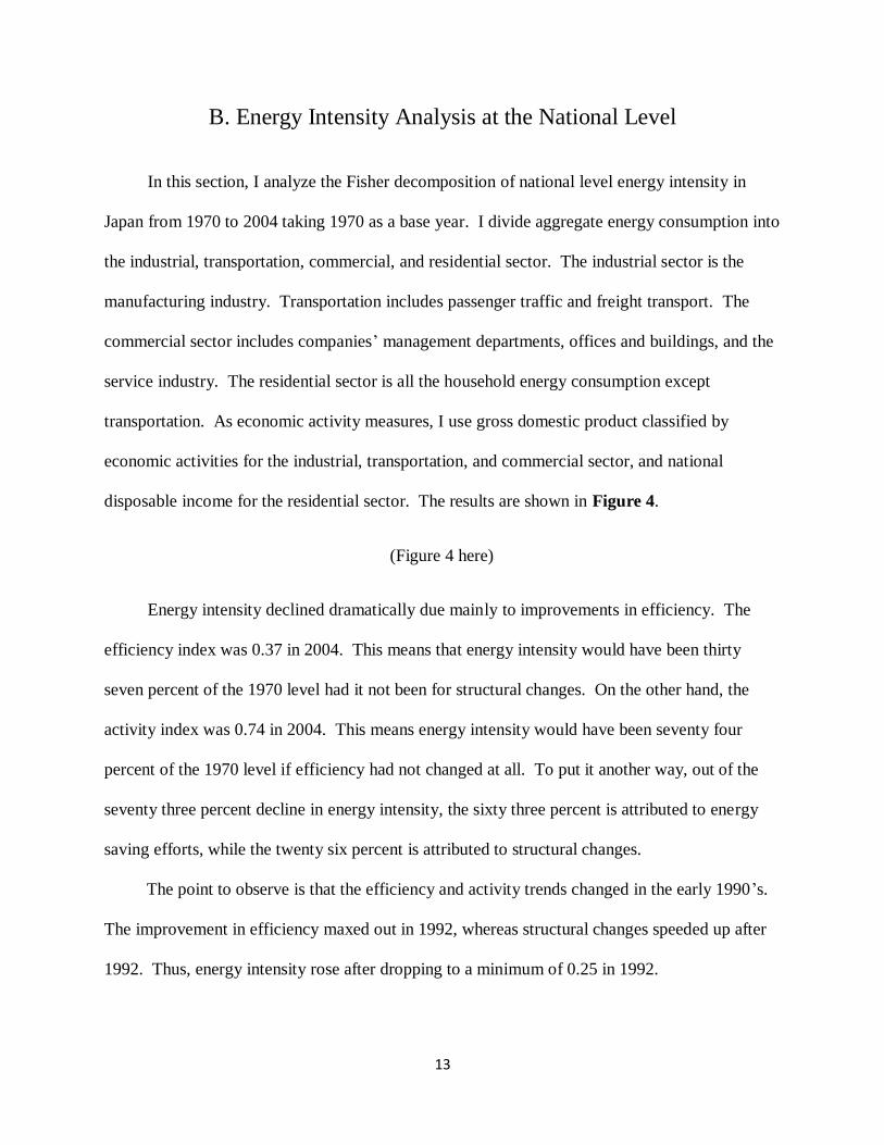
B. Energy Intensity Analysis at the National Level
In this section, I analyze the Fisher decomposition of national level energy intensity in
Japan from 1970 to 2004 taking 1970 as a base year. I divide aggregate energy consumption into
the industrial, transportation, commercial, and residential sector. The industrial sector is the
manufacturing industry. Transportation includes passenger traffic and freight transport. The
commercial sector includes companies’ management departments, offices and buildings, and the
service industry. The residential sector is all the household energy consumption except
transportation. As economic activity measures, I use gross domestic product classified by
economic activities for the industrial, transportation, and commercial sector, and national
disposable income for the residential sector. The results are shown in Figure 4.
(Figure 4 here)
Energy intensity declined dramatically due mainly to improvements in efficiency. The
efficiency index was 0.37 in 2004. This means that energy intensity would have been thirty
seven percent of the 1970 level had it not been for structural changes. On the other hand, the
activity index was 0.74 in 2004. This means energy intensity would have been seventy four
percent of the 1970 level if efficiency had not changed at all. To put it another way, out of the
seventy three percent decline in energy intensity, the sixty three percent is attributed to energy
saving efforts, while the twenty six percent is attributed to structural changes.
The point to observe is that the efficiency and activity trends changed in the early 1990’s.
The improvement in efficiency maxed out in 1992, whereas structural changes speeded up after
1992. Thus, energy intensity rose after dropping to a minimum of 0.25 in 1992.
Page 14
14
C. Energy Intensity Analysis at the Prefecture Level
Before I turn to the decomposition of prefecture level energy intensity, it is useful to be aware
how energy intensity varies between prefectures. One sees from Figure 5 that aggregate energy
intensity in Tokyo is by far the lowest. In prefectures such as Yamaguchi, Oita and Okayama,
aggregate energy intensity is quite high and so is the industrial energy intensity. These
prefectures are all located in Japanese major industrial areas and have many energy intensive
industries, i.e., iron and steel, chemicals, non metallic mineral products, pulp, paper and paper
products industries. Energy intensity in the commercial sector does not vary greatly between
prefectures, though some prefectures are clearly less efficient than the others. In the residential
sector, the trends of energy intensity are quite similar between prefectures. Since Hokkaido,
Aomori and Akita, the northernmost prefectures and Okinawa, the southernmost prefecture, have
the highest energy intensity; there is a fair possibility of the existence of geographical factors.
(Figure 5 here)
For the Fisher decomposition of prefecture level energy intensity in Japan, I use a data set
covering the period from 1990 to 2003 and take 1990 as a base year. I divide aggregate energy
consumption into industrial, commercial, and residential sector. I do not include transportation
as a sector. Data on energy consumption in the transportation industry are not gathered at the
prefecture level, because operations of transportation companies range over many prefectures
and thus their energy consumption cannot be allocated between prefectures. Energy
consumption of household owned cars is included in the residential sector. As economic activity
measures, I use gross prefectural domestic product classified by economic activities for the
industrial and commercial sector, and prefectural income for the residential sector. The results
Page 15
15
appear in Figure 6. It is found that the trends of energy intensity vary between prefectures
because energy efficiency has worsened more in some prefectures than in the others. It is
possible that some energy saving measures have been taken in the prefectures where energy
efficiency has improved; on the other hand, there is little difference in structural changes
between prefectures.
(Figure 6 here)
D. Energy Intensity Analysis at the Sectional Level
From the previous section, the initial reductions in energy consumption can be
attributed mainly to improvements in efficiency. After 1990, the changing of economic activity
had influenced on reduction in energy consumption; on the other hand, the reduction of
aggregate energy intensity in Japan has stopped since 1990. The question we have to ask here is
which sector did not improve energy-efficiency. Importantly, this question offers the key to an
understanding of reducing energy consumption in the future. We can see how the energy
efficiency has changed in each sector since 1990 in Figure 7. As Figure 7 indicates, each sector
has progressively become less energy efficient since 1990. Therefore, policy makers should take
a decision that the each sector carries their share of burden.
(Figure 7 here)
Ⅳ. THE MODEL
From what has been discussed in previous chapters, we may conclude that energy intensity
has slightly increased since early 1990’s. It is also found that all sectors have not increased their
efforts toward energy saving. Now, the Japanese government has begun to discuss proposals of
Page 16
16
environmental taxes in order to reduce carbon emissions. However, the Japanese government
has not figured out the effect of environmental taxes on the economy. Therefore, for policy
makers to adopt appropriate polices, we need to analyze the effect of environmental taxes on the
Japanese economy on regional and national basis.
This chapter presents the economic impacts of policy to mitigate the emission of heat-
trapping greenhouse gases which are carbon dioxide, methane, nitrous oxide and fluorinated
gases. Heat-trapping greenhouse gases contribute to global warming and the most important
heat-trapping greenhouse gas is carbon dioxide.
Carbon dioxide emissions come primarily from the combustion of fossil fuels in energy use.
For instance, on the supply side of the economy, fossil fuels are the large-scale source of energy,
while, on the demand side of the economy, energy is employed as an input to every activity.
Therefore, when policy makers adopt appropriate environmental policies to reduce carbon
dioxide, these policies may cause large increases in energy prices, reduction in energy use, and
declines in economic impacts and welfare.
There are two main polices to achieve emission reduction. One is price instrument which
indicates environmental tax. Second is quantity instrument which indicates an emission cap and
trading system. However, there are some critiques of quantity instrument. Firstly, cap and trade
systems cannot reduce the sum total of carbon emissions in the world. For example, many
developed countries may purchase "hot air" which is surplus credits to pollute held by former
communist countries or developing countries. As a result, there is possibility of increasing the
amount of carbon emission which everyone believes must decrease when cap and trade system is
introduced. Secondly, the government may impose an additional burden on people to finance the
Page 17
17
cost of hot air. This additional burden is no different from environmental taxes. For example,
Japan's emissions climbed around 13 percent in 2005 versus the 1990 level in the latest
government data, leaving it 19 percent off the Kyoto target to cut emissions. Analysts say it will
struggle to meet the target without buying hot air from former communist countries. However,
the Japanese government has no idea how to finance the cost of hot air.
Therefore, this paper only adopts price instrument in order to investigate how much effect the
environmental tax has on the economy.
A. Model structure
I present the structure of the model used for a static price equilibrium simulation of Japanese
economy. This model is refereed to Sue Wing (2004).
Firms are classified into 8 aggregate sectors: coal mining, natural gas distribution, refined
petroleum, electric power, energy-intensive manufacturing (an amalgam of the chemical, ferrous
and non-ferrous metal, pulp and paper, and stone, clay and glass industries), transportation,
service and the remaining manufacture. Labor and capital are the primary factors. Each firms
produce output from capital, labor and intermediate inputs (energy goods and non energy goods),
according to nested CES production functions which is referred to Bosetti et al. (2006). To put it
more concretely, the output of the j-th industry, yj, is combining N types of intermediate goods
imput, x, E types of fossil fuel commodities, e, capital input, K, and labor input, L, according to
the nested CES production function:
Page 18
18
yj =
βj
klem yjkle
(σ jklem −1)
σ jklem
γi,jklem x
i,j
(σ jklem −1)
σ jklem
Ni=1
σ jklem
(σ jklem −1)
(9)
yjkle =
βj
kle yjkl
(σ jkle −1)
σ jkle
+ γe,jkleE
e=1 ee,j
(σ jkle −1)
σ jkle
σ jkle
σ jkle −1
(10)
yjkl =
βj
kl Kj
(σ jkl −1)
σ jkl
+ γjkl L
j
(σ jkl −1)
σ jkl
σ jkl
(σ jkl −1)
(11)
where βi,j and γf,j are the technical coefficients, while σj denotes each industry’s elasticity of
substitution. Moreover yjkl is composite goods of capital and labor, and yj
kle is composite goods
of capital-labor and energy goods.
Households differ in their preferences. For example, Hokkaido, the northernmost prefecture
in Japan, has lots of snow. As a result, people living there may use more electricity during
winter than those who are in warmer regions. Thus, preference of people living in Hokkaido is
different from preference of people living in other regions. This paper divides Japan into 8
regions in order to take several households with different preference into consideration.
Page 19
19
There are three types of household demand for commodities of final uses: consumption,
investment, and net exports. Investment and net exports are assumed to be exogenous and
constant. Households in each region are modeled as a utility-maximizing representative agent
with CES preferences over their consumption of commodities. Consumption is financed out of
the income which each regional agent receives from the rental of their endowments of labor and
capital to industries. To put it more concretely, the j-th household utility, Uj , is related to the
consumption, c, of the N commodities by the CES function:
Uj = αi,jCj
(ω−1)ω N
i=1
ω(ω−1)
(12)
where αi,j’s are the technical coefficients of the utility function, and ω is the elasticity of
substitution.
An important feature is that this model uses revenues accruing from environmental taxes in
order to reduce pre-existing distortions brought by pre-existing distorting taxes. Several studies
have been made on the possibility of substituting environmental taxes for pre-existing distorting
taxes in order to lower the efficiency cost. This approach is referred to as “revenue recycling.”
This paper assumes that pre-existing ad-valorem taxes on production and imports bring about
pre-existing distortions. Under these situations, imposing environmental taxes may leave the
economy worse. Now, policy makers need to maximize gains in economic efficiency. So I
assume that the revenue, raised by pre-existing ad-valorem taxes on production and imports, is
recycled to the representative agent in a lump sum.
Page 20
20
B. Data
For the benchmark dataset, I use Japanese input-output tables for the year 2000 provided by
Japanese Ministry of Internal Affairs and Communications. The data of CO2 emissions in the
year 2000 from coal, petroleum and natural gas are obtained by Greenhouse Gas Inventory
Office in Japan. Following Sue Wing (2004), this paper assumes that both σj’s, each industry’s
elasticity of substitutions, and ω, elasticity of substitution, are 1.
C. Environmental taxes
The model attempts to simulate the effect of imposing environmental taxes on emission of
CO2. To calculate the burden of environmental taxes on industries and the representative agent,
it is necessary to examine the relationship between the levels of production and demand activities
and the quantity of emissions. This is because it is difficult to correctly grasp how much CO2
each sector emits. Therefore, instead of directly imposing environmental taxes on the activity
emitting CO2, it is better to impose environmental taxes on fossil fuel commodities when these
commodities are traded in the market. The simplest way of doing this is to assume a fixed
relationship between the aggregate demands for fossil fuel commodities in which carbon is
embodied, such as coal, refined petroleum and natural gas. Therefore, a tax on carbon results in
a set of commodity taxes that are differentiated by energy goods’ carbon contents, and acts to
increase the gross-of- advalorem-tax price of each fossil fuel.
The model is simulated to reproduce the benchmark as a baseline no-policy case. Next, I
constructed a series of counterfactual shocks by levying carbon taxes that range between $3/ton
and $12/ton CO2, in order to attain the Kyoto protocol. According to Sue Wing (2004), “a
Page 21
21
potential source of confusion in that GHG taxes are usually specified in units of carbon while
environmental statistics usually account for GHG emissions in units of CO2. The ratio of these
substances’ molecular weights (0.273 tons of carbon per ton of CO2) establishes an equivalency
between the two measures.” Therefore, the values of a tax on carbon become equivalent to taxes
on CO2: $0.819, $1.638, $2.457 and $3.276 per ton of CO2 respectively.
D. Result
In this section, I present results from the numerical analysis. In order to attain the Kyoto
Protocol, Japan has to reduce carbon emissions by six percent compared to 1990 emissions level.
CO2 emissions in the year 1990 were 1,144 MT. Therefore, Japan has to reduce CO2 emissions
to 1,079 MT.
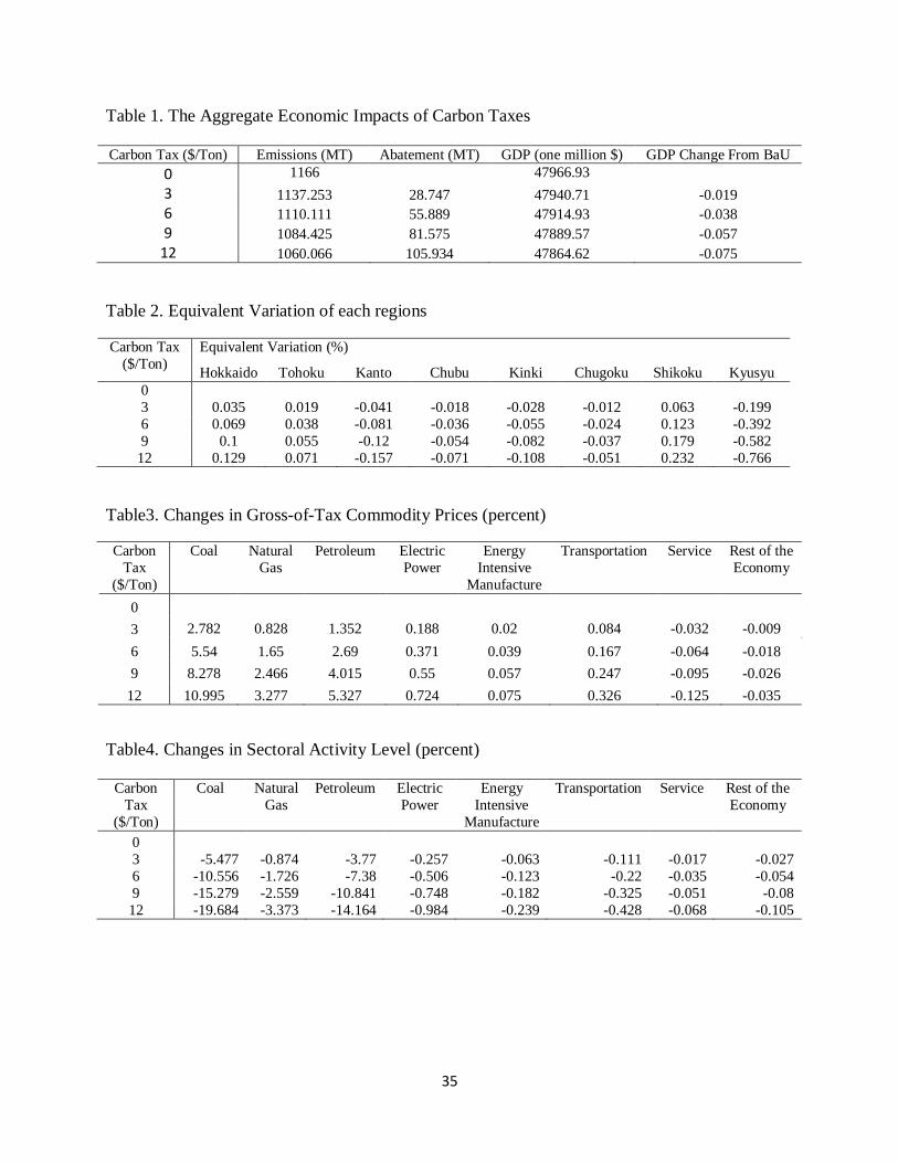
The model simulates the effects of imposing range of additional taxes on emissions of CO2.
Table 1 shows the impact of CO2 reduction on GDP. In order to reduce CO2 emissions to 1,079
MT, the Japanese government needs to impose a $12/ton tax. A 7 percent fails in GDP.
This model assumes that ad-valorem taxes on production are levied on the output of each
industry. Also, these taxes discourage economically desirable activities. Now, this paper
assumes that the central government collects tax revenue and allocates it to each household
evenly as a lump-sum supplement to the income, because the central government’s imposing
environmental taxes cause to raise the tax burden ratio.
(Table 1 here)
To capture aggregate impact of policies, I use Equivalent variations because this indicator is
one of the well micro-founded indicators. This result appears in Table2.
Page 22
22
Equivalent variations of Hokkaido region, Tohoku region and Shikoku region are positive.
This means that revenue from pre-existing production taxes offsets the cost of environmental
taxes. On the other hand, equivalent variations of other regions are negative. This means that
revenue from pre-existing production taxes could not offset the cost of environmental taxes.
Let us look at this result from a different angle. Equivalent variations of Kanto region and
Kinki region decrease to more than 10 percent. A plausible explanation of this is Kanto region
and Kinki region are urban regions. Therefore people who live there are more dependent on
energy commodities than those who live in rural regions. In other words, Hokkaido region,
Tohoku region and Shikoku region are rural regions. Therefore people who live there may not
be dependent on energy commodities than people who live in urban regions.
(Table 2 here)
Table 3 shows how much carbon tax raises the consumer price. Increase in consumer price of
coal is higher than increases in consumer price in any other sectors. A $3/ton carbon tax raises
the consumer price of coal by 3 percent, and a $12/ton carbon tax raises the consumer price of
coal by 11 percent. This is because coal is the most carbon-intensive energy source compared
with other energy sources, such as oil and gas.
(Table 3 here)
Table 4 indicates changes in final consumption by commodities. Table 5 shows changes in
sectoral activity level. The changes in final consumption of commodities and in sectoral activity
levels correspond closely to changes in gross-of-tax commodity prices (Table 3).
(Table 4 and Table 5 here)
Page 23
23
Also the impacts of environmental policy interventions on pollution are investigated by CGE
model. Figure 8 shows emissions from each sector. In order to reduce carbon emission by six
percent compared with 1990 emissions levels, the Japanese CO2 target is 1,079 MT. As
mentioned above, in order to reduce CO2 emissions to 1,079 MT, the Japanese government
needs to impose a $12/ton tax. The coal sector and the oil sector reduce the carbon emission by
around 30 percent, while other sectors reduce the carbon emission by less than 10 percent.
(Figure 8 here)
E. Sensitivity Analysis
To test the generality of the result above, I have run a series of sensitivity analysis. In order
to test the accuracy of this model, we need two criterions. First criteria is that when the elasticity
of substitution is changed, the direction of change in each production is unchanged. Second
criteria is that when the elasticity of substitution is changed, the order of change in each
production is still the same.
Although the model assumes that the elasticity of substitution for the CES production
function between input commodities and energy commodities is 1, in order to investigate
robustness, I conducted experiments with the elasticity of substitution for the CES production
function between input commodities and energy commodities is 0.8 and 1.2, respectively. This
analysis results in Table 6. Table 6 clearly shows that the results of simulations are reliable
because both of criterions are satisfied.
(Table 6 here)
Page 24
24
Ⅴ. CONCLUSION
In conclusion, I would like to state the following two points. Firstly, I applied the energy
intensity decomposition method with the Fisher Ideal index to Japanese energy intensity. It is
found that at the national level, energy intensity declined by seventy three percent from 1970 to
2003. Furthermore, the sixty three percent of the decline is attributed to improvement in energy
efficiency. Energy intensity, however, has slightly increased since early 1990’s. The results
show that at the prefecture level, improvements in energy intensity have not been uniform after
1990. It is also found that each sector has to put more effort in order to reduce carbon emissions
by six percent compared to 1990 emissions level.
Secondly, this paper explores the potential impact reduction of carbon emission on the
economy. I find that the Japanese government needs to enact the environmental taxes on a
$12/ton in order to meet the Kyoto Protocol. It is also found that imposing a $12/ton
environmental tax reduces Japanese GDP by around six percent and equivalent variations in
urban regions fall while equivalent variations in rural regions rise.
Finally, I point out several future research directions. First, the model is static which means
that static models cannot deal with issues of next periods. This model assumes that investment
demand of each commodity is fixed. However, a more realistic model, like dynamic models,
would let households adjust saving and investment behavior to a tax shock, due to the forward-
looking behavior of households. Therefore, this simple static general equilibrium model needs
to be transformed into a dynamic model.
Page 25
25
Second, the economy’s net export position is assumed to be constant. I need to extend this
model into a small open economy model in order to model the economy’s net export position as
an endogenous variable. One way to extend this model is that we let imports and exports linked
by the balance-of-payment condition and assume that imports and domestically supplied goods
are aggregated to be Armington’s (1969) composite goods.
Lastly, we have to consider how the central government allocates revenue from pre-existing
production taxes to each region. This paper evenly distributes revenue from pre-existing
production taxes to each region. However, each region has a different economics situation. For
example, some regions pay more production taxes than other regions. Therefore policy makers
have to consider how they can fairly distribute revenue from pre-existing production taxes to
each region.
Page 26
26
REFERENCES
-Armington. P.S. A Theory of Demand for Products Distinguished by Place of Production.
IMF Staff Papers 1969;16(1);170-201.
-Balisteri. E.J., Reilly. J.M., and Jacoby H.D. Assessing the state-level burden of carbon
emissions abatement. Mimeo 2004.
-Bosetti. V., Carraro. C., Galeotti. M., and Tavoni. M. WITCH. A World Induced Technical
Change Hybrid Model. The Energy Journal 2006;27(2);13-38.
-Boyd. G.A., J.F. McDonald., M. Ross., and D. Hanson. Separating the Changing Composition
of U.S. Manufacturing Production from Energy Efficiency Improvement; A Divisia Index
Approach. The Energy Journal 1987;8(2); 77-96.
-Boyd. G. A., and Roop. J.M. A note on the Fisher Ideal Index Decomposition for Structural
Change in Energy Intensity. The Energy Journal 2004;25; 87-101.
-Diewert.W.E. The Consumer Price Index and Index Number Theory; A Survey.
2001;Vancouver, Department of Economics, University of British Columbia, Department
Paper 0102.
-Fisher. I. The Best Form of Index Number. Quarterly Publications of the American Statistical
Association 1921;17; 533-37.
Page 27
27
-Li. P.C. and Rose. A.Z. Global warning policy and the Pennsylvania economy: A computable
general equilibrium analysis. Economic System Research 1995;7;151-171.
-Partridge. M.D. and Rickman. D.S. Regional computable general equilibrium modeling: A
survey and critical appraisal. International Regional Science Review 1998; 3;205-250.
-Ross. M.T., Beach. R.T. and Murray. B.C. Distributional implications of regional climate
change policies in theU.S.: A general equilibrium assessment.; 2004; Working paper.
-Sue Wing I. The Regional Impact of U.S. Climate Change Policy:a general equilibrium
Analysis.2007; Working paper.
-Sue Wing I. Computable General Equilibrium Models and Their Use in Economy-Wide Policy
Anaysis. MIT Joint Program on the Science and Policy of Global Change;2004;Technical Note
No.6.
-Okajima. S. Analysis of Energy intensity in Japan. 2008; Working paper.
Page 28
28
Figure 1 Japan's Aggregate Energy Consumption
Energy
Consumption
Annual Percent
Change
0
2,000
4,000
6,000
8,000
10,000
12,000
14,000
16,000
18,000
1965 1970 1975 1980 1985 1990 1995 2000
Year
En
erg
y C
on
sum
pti
on
(P
J)
-10
-5
0
5
10
15
20
25
An
nu
al P
erce
nt
Ch
ang
e (%
)
Rapid
Economic
Growth Oil Crises
Bubble
EconomyEconomic
Stagnation
(Agency for Natural Resources and Energy)
Page 29
29
Figure 2 Japan's Energy Consumption by Energy Consuming Sectors
Industrial
Transportation
Commercial
Residential
0
1,000
2,000
3,000
4,000
5,000
6,000
7,000
8,000
1965 1970 1975 1980 1985 1990 1995 2000
Year
En
erg
y C
on
sum
pti
on
(P
J)
The industrial sector is the manufacturing industry. The transportation sector
includes passenger traffic, such as cars and buses, and freight transport, such as land
transportation, shipping and airfreight. The commercial sector includes companies ’
management departments, offices and buildings, and the service industry. The
residential sector is all the household energy consumption except transportation, such
as private cars.
(Agency for Natural Resources and Energy)
Page 30
30
Figure 3 Japan's Energy Consumption and GDP Trends
0
50
100
150
1965 1970 1975 1980 1985 1990 1995 2000
Year
En
erg
y C
on
sum
pti
on
Per
GD
P
(GJ/
1,0
00
,00
0Y
en)
En
erg
y C
on
sum
pti
on
Per
Cap
ita
(GJ/
Per
son
)
0.0
1.0
2.0
3.0
4.0
5.0
GD
P P
er C
apit
a (1
,00
0,0
00
Yen
/Per
son
)
Energy Consumption Per GDP
Energy Consumption
Per Capita
GDP Per Capita
(Ministry of Internal Affairs and Communications, Cabinet Office, Agency for Natural
Resources and Energy)
Page 31
31
Figure 4 Decomposition of Aggregate Energy Intensity at the National Level
0.0
0.2
0.4
0.6
0.8
1.0
1.2
1970 1975 1980 1985 1990 1995 2000Year
En
erg
y I
nte
nsi
ty (
19
70
=1
)
Activity Index
0.74
Efficiency Index
0.37
Energy Intensity
0.27
Page 32
32
Figure 5 Ten Prefectures with the Lowest and Highest Energy Intensity
(1) Aggregate Energy Intensity
0
20
40
60
80
100
1990 1995 2000
Year
Ener
gy
Inte
nsi
ty (
GJ/
1,0
00,0
00
Yen
)
Wakayama
Tokyo
OsakaKyoto
NaganoNagasaki
Ehime
Okayama
Oita
Yamaguchi
Mean
(2) Industrial Energy Intensity
0
40
80
120
160
200
1990 1995 2000
Year
En
erg
y I
nte
nsi
ty (
GJ/
1,0
00
,00
0Y
en)
TokyoKyotoNaganoNara
Yamagata
EhimeChiba
Okayam
a
Oita
Yamaguchi
Mean
(3) Commercial Energy Intensity
0
5
10
15
20
25
1990 1995 2000
Year
Ener
gy
Inte
nsi
ty (
GJ/
1,0
00,0
00
Yen
)
Tokyo
NiigataOkayam
aShizuokaKanaga
wa
Yamagat
a
Yamanas
hi
Okinawa
Ibaraki
Tottori
Mean
(4) Residential Energy Intensity
0
4
8
12
16
20
1990 1995 2000
Year
Ener
gy
Inte
nsi
ty (
GJ/
1,0
00,0
00
Yen
)
Tokyo
ShigaAichiIbarakiTochigi
OkinawaAkitaKochiHokkaidoAomori
Mean
Page 33
33
Figure 6 Decomposition of the Prefecture Level Energy Intensity: Ten Prefectures with the
Most and Least Reduced Energy Intensity, Efficiency and Activity.
(1) Energy Intensity Index Trend
0.0
0.2
0.4
0.6
0.8
1.0
1.2
1.4
1990 1995 2000Year
En
erg
y I
nte
nsi
ty (
19
90
=1
)
Wakayama TottoriOita YamanashiOkayama AkitaMie NaraFukuoka Tochigi
(Worst 5)(Best 5)
(2) Efficiency Index Trend
0.0
0.2
0.4
0.6
0.8
1.0
1.2
1.4
1990 1995 2000Year
Eff
icie
ncy
(1
99
0=
1)
Wakayama AkitaTokushima TottoriOita AomoriMie YamanashiShizuoka Nara
(Worst 5)(Best 5)
(3) Activity Index Trend
0.0
0.2
0.4
0.6
0.8
1.0
1.2
1.4
1990 1995 2000Year
Act
ivit
y (
19
90
=1
)
Chiba TokyoHyogo TokushimaKanagawa OkinawaOkayama ShizuokaEhime Tottori
(Worst 5)(Best 5)
Page 34
34
Figure 7 Energy Efficiency of each sectors
0
0.2
0.4
0.6
0.8
1
1.2
1.4
1990 1991 1992 1993 1994 1995 1996 1997 1998 1999 2000 2001 2002 2003
Eff
icie
ncy
(199
0=1
)
Year
industry
residential
service
Page 35
35
Table 1. The Aggregate Economic Impacts of Carbon Taxes Carbon Tax ($/Ton) Emissions (MT) Abatement (MT) GDP (one million $) GDP Change From BaU
0 1166 47966.93 3 1137.253 28.747 47940.71 -0.019
6 1110.111 55.889 47914.93 -0.038
9 1084.425 81.575 47889.57 -0.057
12 1060.066 105.934 47864.62 -0.075
Table 2. Equivalent Variation of each regions
Carbon Tax
($/Ton)
Equivalent Variation (%)
Hokkaido Tohoku Kanto Chubu Kinki Chugoku Shikoku Kyusyu
0
3 0.035 0.019 -0.041 -0.018 -0.028 -0.012 0.063 -0.199
6 0.069 0.038 -0.081 -0.036 -0.055 -0.024 0.123 -0.392
9 0.1 0.055 -0.12 -0.054 -0.082 -0.037 0.179 -0.582
12 0.129 0.071 -0.157 -0.071 -0.108 -0.051 0.232 -0.766
Table3. Changes in Gross-of-Tax Commodity Prices (percent)
Carbon
Tax
($/Ton)
Coal Natural
Gas
Petroleum Electric
Power
Energy
Intensive
Manufacture
Transportation Service Rest of the
Economy
0 3 2.782 0.828 1.352 0.188 0.02 0.084 -0.032 -0.009
6 5.54 1.65 2.69 0.371 0.039 0.167 -0.064 -0.018
9 8.278 2.466 4.015 0.55 0.057 0.247 -0.095 -0.026
12 10.995 3.277 5.327 0.724 0.075 0.326 -0.125 -0.035
Table4. Changes in Sectoral Activity Level (percent)
Carbon
Tax
($/Ton)
Coal Natural
Gas
Petroleum Electric
Power
Energy
Intensive
Manufacture
Transportation Service Rest of the
Economy
0 3 -5.477 -0.874 -3.77 -0.257 -0.063 -0.111 -0.017 -0.027
6 -10.556 -1.726 -7.38 -0.506 -0.123 -0.22 -0.035 -0.054
9 -15.279 -2.559 -10.841 -0.748 -0.182 -0.325 -0.051 -0.08
12 -19.684 -3.373 -14.164 -0.984 -0.239 -0.428 -0.068 -0.105
Page 36
36
Table5. Changes in Final Consumption by Commodity (percent)
Carbon
Tax
($/Ton)
Coal Natural
Gas
Petroleum Electric
Power
Energy
Intensive
Manufacture
Transportation Service Rest of the
Economy
0
3 -2.753 -0.868 -1.381 -0.235 -0.067 -0.132 -0.015 -0.039
6 -5.339 -1.716 -2.712 -0.464 -0.133 -0.261 -0.031 -0.077
9 -7.775 -2.544 -3.995 -0.687 -0.197 -0.387 -0.046 -0.114
12 -10.073 -3.353 -5.234 -0.903 -0.26 -0.51 -0.061 -0.151
Table6. Sensitivity Results
Elasticity=1 Elasticity=1.2 Elasticity=0.8
Coal -19.684 -21.088 -18.246
Petroleum -14.164 -15.726 -12.57
Natural Gas -3.373 -3.628 -3.113
Electric Power -0.984 -1.404 -0.556
Transportation -0.428 -0.479 -0.377
Energy Intensive Manufacture -0.239 -0.277 -0.202
Rest of the Economy -0.105 -0.122 -0.088
Service -0.068 -0.086 -0.049
Page 37
37
Figure8. Impact of Carbon Taxes on Carbon Emissions by Sector
0
200
400
600
800
1000
1200
1400
0 3 6 9 12
Car
bon
Dio
xid
e E
mis
sion
s (M
T)
Carbon Taxe ($/Ton Carbon)
Impact of Carbon Taxes on Carbon Emissions by Sector
hhold
roe
service
trn
eis
ele
oil
gas
col