Analysis of the Structural Integrity of a Floating Semisubmersible

Foundation for Offshore Wind

Diogo Rosario Diasdiogo.r.dias@tecnico.ulisboa.pt

Instituto Superior Tecnico, Universidade de Lisboa, Portugal

November 2017

Abstract

Floating wind power is a promising solution to the expansion of offshore wind, as it can be used indeeper water as well as it allows the usage of large wind turbines. Nonetheless, this technology is stillin demonstration, with just a few full-scale prototypes all over the world. On this thesis the structuralintegrity of a semisubmersible floating foundation for offshore wind is studied, which foundation wascreated within the DeepCwind consortium in order to validate aero-hydro-servo-elastic numerical codes.Thereby, the focus is on the development of an appropriate numerical model for the structural analysisof the foundation. FAST 8, an aero-hydro-servo-elastic numerical code, was used to obtain the variousloads applied on the structure. These loads were preprocessed before their input on a finite elementmodel developed using ANSYS software. A submodeling technique was used to analyse with moreprecision and detail the stress concentration regions of the structure. Static and transient structuralanalysis allowed to find critic regions of the foundation and hence begin an iterative reinforcementprocess, allowing the study of the structure’s suitability for use in offshore environments. Moreover, amodal analysis and a hydrodynamic response analysis of both the original and reinforced structureswere made and their results compared. Results show that the DeepCwind floating semisubmersiblecannot stand the severe offshore environment it was designed to.

Keywords: offshore wind power, floating, semisubmersible, DeepCwind, structural analysis, finiteelements, submodeling

1 INTRODUCTION

Offshore wind turbines are a leading renewable en-ergy technology capable of supporting a low-carboneconomy in world. The offshore wind industry re-lies essentially on fixed-base foundations such asmonopiles, space frame jackets and tripods, whoseuse is limited to shallow waters, thereafter limitingthe growth of this industry. Since floating offshorewind foundations are not limited by water depth,they are a solution with great prospect to unlockthe full-potential of the offshore wind market [6].

A typical floating wind turbine comprises a rotornacelle assembly, a tower, a foundation and a moor-ing system. Since they are floating structures, theyhave 6 DOF. According to Butterfield et al. [5], theycan be classified by three main physical principlesused to archive stability. Thus, Spar-type rely onballasting, TLP count on the mooring lines tension,and semisubmersible makes use of the distributedbuoyancy, taking advantage of the weighted waterplane area. The latter is the case of the studiedfoundation, although it also uses ballasting as a

secondary source of stability. In reality, all foun-dations achieve stability from the three presentedprinciples, but rely in one as the main source.

The foundation subjected to analysis was thefloating semisubmersible foundation examined inthe OC4-project (Offshore Code Comparison Col-laboration Continuation) whose design was origi-nated from the activities of the DeepCwind con-sortium, in order to verify the floating capabil-ities of various aero-hydro-servo-elastic numericalcodes [12, 20, 21]. This foundation uses the NREL5 MW Reference wind turbine [19], described inRef. [10].

Although multi-body formulations based onbeam elements are a common practice [14], the useof shell elements allows for a more detailed mod-elling of structure [14]. Shell elements were used ona global model of the structure.

To model the loads on the foundation and moor-ing lines computational fluid dynamics models(CFD) can be used, as well as potential flow theo-ries and Morison’s equation, or even a hybrid modelmade of a combination of the latter two.

1

In agreement with GL guidelines for offshorewind power [1], various DLC (design load cases)have to be considered. Nevertheless, this analysiswas based on DLC 1.1 to find critic regions and testalternative solutions.

2 MODEL DEFINITION

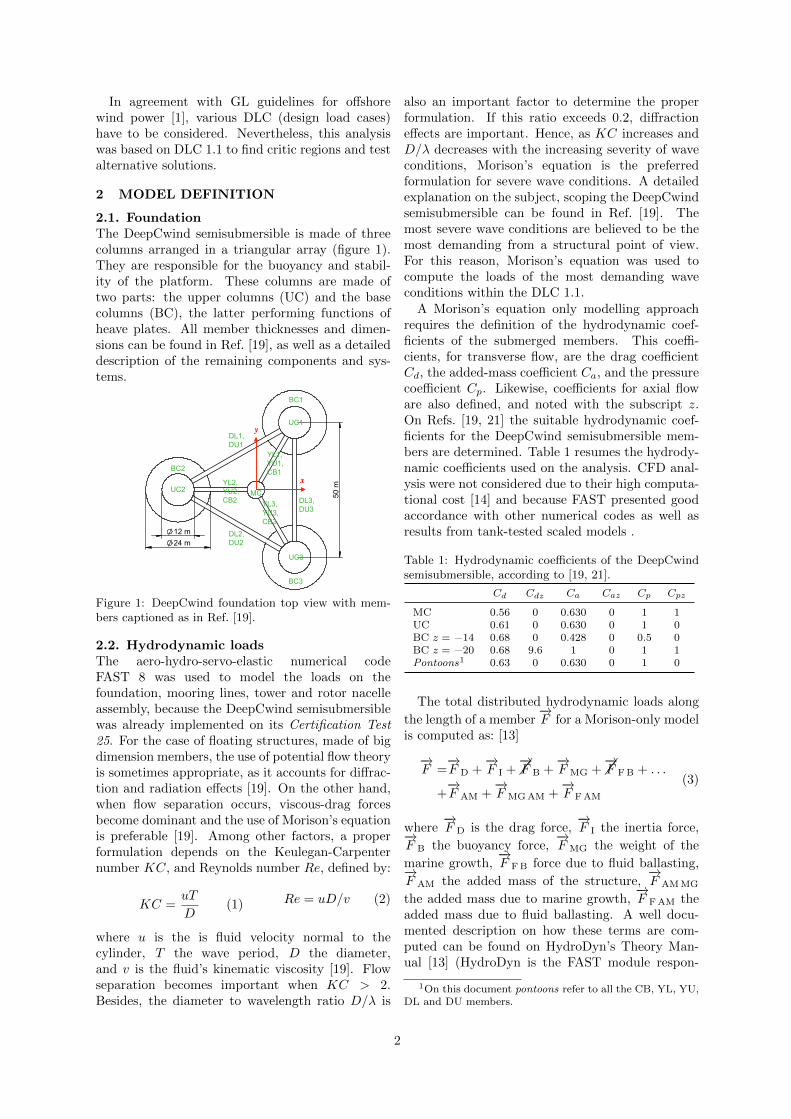
2.1. FoundationThe DeepCwind semisubmersible is made of threecolumns arranged in a triangular array (figure 1).They are responsible for the buoyancy and stabil-ity of the platform. These columns are made oftwo parts: the upper columns (UC) and the basecolumns (BC), the latter performing functions ofheave plates. All member thicknesses and dimen-sions can be found in Ref. [19], as well as a detaileddescription of the remaining components and sys-tems.

6

24

m

DeepCwind foundation, tower and turbine NREL 5MW

50

m

24 m 12 m

20

m

A A

B B

C C

D D

E E

F F

8

8

7

7

6

6

5

5

4

4

3

3

2

2

1

1

DRAWN

CHK'D

APPV'D

MFG

Q.A

UNLESS OTHERWISE SPECIFIED:DIMENSIONS ARE IN MILLIMETERSSURFACE FINISH:TOLERANCES: LINEAR: ANGULAR:

FINISH: DEBURR AND BREAK SHARP EDGES

NAME SIGNATURE DATE

MATERIAL:

DO NOT SCALE DRAWING REVISION

TITLE:

DWG NO.

SCALE:1:2000 SHEET 1 OF 1

A3

WEIGHT:

Assembly_DeepCwind_Desenho

SWL

wind

z

x

y

DL3,DU3

DL1,DU1

DL2,DU2

UC1

MCUC2

BC2

BC3

UC3

YL1,YU1,CB1

YL2,YU2,CB2 YL3,

YU3,CB3

BC3

UC3

BC2

UC2 MC

DL1,DL2

DU1,DU2

CB2

CB3

26

BC1

x

Figure 1: DeepCwind foundation top view with mem-bers captioned as in Ref. [19].

2.2. Hydrodynamic loadsThe aero-hydro-servo-elastic numerical codeFAST 8 was used to model the loads on thefoundation, mooring lines, tower and rotor nacelleassembly, because the DeepCwind semisubmersiblewas already implemented on its Certification Test25. For the case of floating structures, made of bigdimension members, the use of potential flow theoryis sometimes appropriate, as it accounts for diffrac-tion and radiation effects [19]. On the other hand,when flow separation occurs, viscous-drag forcesbecome dominant and the use of Morison’s equationis preferable [19]. Among other factors, a properformulation depends on the Keulegan-Carpenternumber KC, and Reynolds number Re, defined by:

KC =uT

D(1) Re = uD/v (2)

where u is the is fluid velocity normal to thecylinder, T the wave period, D the diameter,and v is the fluid’s kinematic viscosity [19]. Flowseparation becomes important when KC > 2.Besides, the diameter to wavelength ratio D/λ is

also an important factor to determine the properformulation. If this ratio exceeds 0.2, diffractioneffects are important. Hence, as KC increases andD/λ decreases with the increasing severity of waveconditions, Morison’s equation is the preferredformulation for severe wave conditions. A detailedexplanation on the subject, scoping the DeepCwindsemisubmersible can be found in Ref. [19]. Themost severe wave conditions are believed to be themost demanding from a structural point of view.For this reason, Morison’s equation was used tocompute the loads of the most demanding waveconditions within the DLC 1.1.

A Morison’s equation only modelling approachrequires the definition of the hydrodynamic coef-ficients of the submerged members. This coeffi-cients, for transverse flow, are the drag coefficientCd, the added-mass coefficient Ca, and the pressurecoefficient Cp. Likewise, coefficients for axial floware also defined, and noted with the subscript z.On Refs. [19, 21] the suitable hydrodynamic coef-ficients for the DeepCwind semisubmersible mem-bers are determined. Table 1 resumes the hydrody-namic coefficients used on the analysis. CFD anal-ysis were not considered due to their high computa-tional cost [14] and because FAST presented goodaccordance with other numerical codes as well asresults from tank-tested scaled models .

Table 1: Hydrodynamic coefficients of the DeepCwindsemisubmersible, according to [19, 21].

Cd Cdz Ca Caz Cp Cpz

MC 0.56 0 0.630 0 1 1UC 0.61 0 0.630 0 1 0BC z = −14 0.68 0 0.428 0 0.5 0BC z = −20 0.68 9.6 1 0 1 1Pontoons1 0.63 0 0.630 0 1 0

The total distributed hydrodynamic loads along

the length of a member−→F for a Morison-only model

is computed as: [13]

−→F =−→F D +

−→F I + ��

−→F B +

−→F MG + ��

−→F FB + . . .

+−→F AM +

−→F MGAM +

−→F FAM

(3)

where−→F D is the drag force,

−→F I the inertia force,−→

F B the buoyancy force,−→F MG the weight of the

marine growth,−→F FB force due to fluid ballasting,−→

F AM the added mass of the structure,−→F AMMG

the added mass due to marine growth,−→F FAM the

added mass due to fluid ballasting. A well docu-mented description on how these terms are com-puted can be found on HydroDyn’s Theory Man-ual [13] (HydroDyn is the FAST module respon-

1On this document pontoons refer to all the CB, YL, YU,DL and DU members.

2

sible for the hydrodynamic problem). An equiva-lent strip-theory formula exists for the case of theBC (heave plates), as well as an adapted Morison’sequation, which can the latter be found in [19]. Thedrag and inertia terms are computed with the Mori-son’s equation. Drag and inertia terms related tomarine growth allow for different hydrodynamic co-efficients, even though that was not made due to in-sufficient data. The Morison’s-only approach usedcomputes buoyancy changes due to platform move-ments using a linearized model [13, 19]. Therefore,FAST computes the total load on the foundationfrom linear hydrostatics, Fhidri , according to theequation 4, written in Einstein’s notation:

Fhidri (q) = ρgV0δi3 − Chidrij qj (4)

where ρ is the fluid’s density, g is the gravitationalacceleration, V0 is the displaced volume of fluidwhen the platform is in its undisplaced position, δi3is the (i, 3) component of the Kronecker-Delta func-tion (i.e. identity matrix), Chidri,j is the (i, j) com-ponent of the linear hydrostatic restoring matrix atthe centre of buoyancy, and qj is the jth platformDOF2 [19]. The original foundation has the follow-ing hydrostatic restoring matrix:

Chidr3,3 = 3.836× 106 N m−1

Chidr4,4 = 1.074× 109 N m rad−1

Chidr5,5 = 1.074× 109 N m rad−1

(5)

For all other values of the indices i, j, Chidrij = 0.

2.3. Aerodynamic loadsFAST’s Aerodyn module computes the aerody-namic loads with the Blade Element Method [16],one of the most used methods for stationary flows.As the real flow is not stationary, Aerodyn usessome corrective measures to include some importantunsteady flow effects, like the stall phenomenon andvortex shedding [8, 16].

2.4. Mooring system loadsMoorDyn module is used to model the mooring sys-tem, since it accounts for non-linear mooring dy-namics. The model uses finite elements, and itconsiders mooring lines inertia, stiffness, internaldamping, buoyancy, hydrodynamic inertia and dragloads, and soil interaction. It does not account forbending stiffness of the lines. A detailed descriptionof this model can be found in Ref. [7].

2.5. Design load case 1.1GL guideline for offshore wind turbines [1] requiresthe study of various DLC to guarantee their certi-fication, which the external conditions have to be

2subscripts i and j range from 1 to 6, one for each plat-form DOF (1 = surge, 2 = sway, 3 = heave, 4 = roll, 5 =pitch, 6 = yaw)

chosen according to a specific installation site. Fora first approach, it has been considered only DLC1.1. The site chosen was the same of Ref. [11]. Ta-ble 2 presents the external conditions for the casesanalysed.

Table 2: External conditions for DLC 1.1 cases anal-ysed. u is the mean wind velocity at hub hight, Hs thesignificant wave height, and Tp the peak period of thesea state.

Case u [m s−1] Hs [m] Tp [s]

1 11.4 2.466 13.1592 18.0 4.005 14.1293 24.0 5.585 16.162

TurbSym was used to create the wind fieldsneeded for the analysis with IEC Kaimal spec-tra and NTM (Normal Turbulence Model), seeRefs. [9, 18]. Airy model with Pierson-Moscowitzspectral density was chosen to model the wave con-ditions, see Ref. [13]. Wind induced sea super-ficial currents were also considered according toIEC 61400-3 standard [9].

As mentioned before, due to the Morison’s equa-tion approach limitations, only severe wave con-ditions were considered. They correlate to higherwind speeds, and for this reason, only externalconditions from rated to cut-out wind speeds weretaken into account.

3 IMPLEMENTATION

3.1. FAST outputs

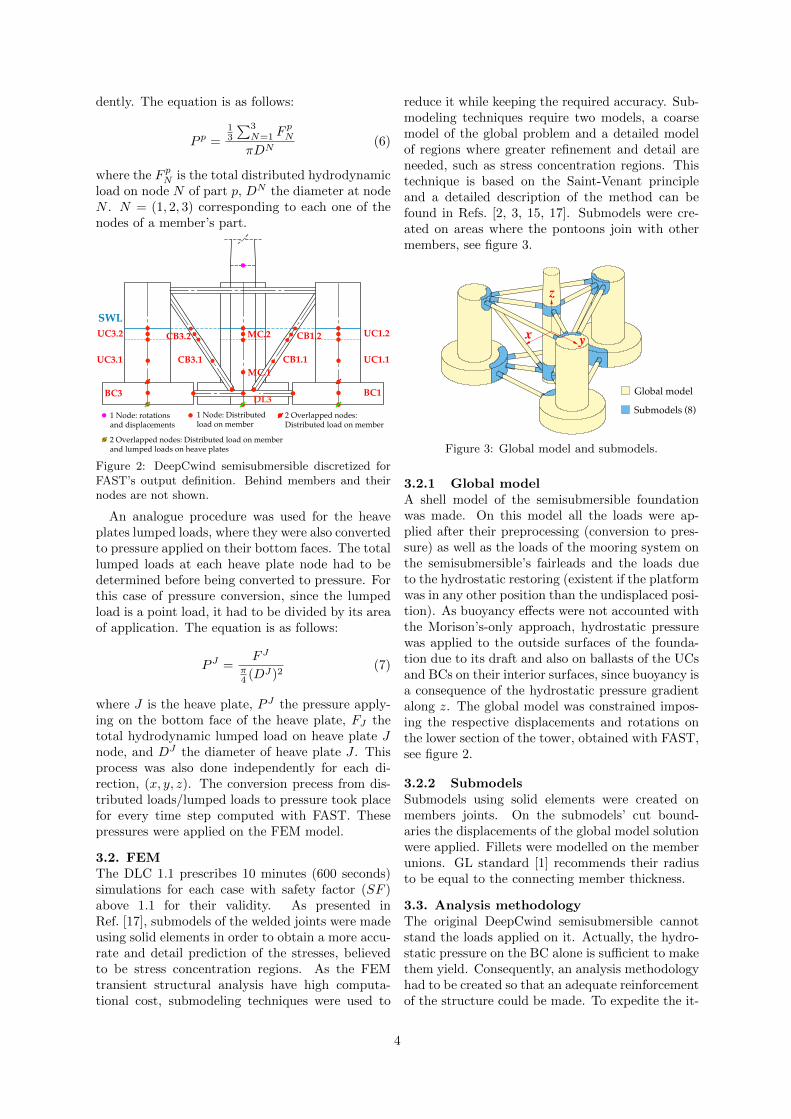
Because hydrodynamic loads decay exponentiallywith depth [13], the DeepCwind semisubmersiblewas discretized through an imaginary horizontalplane 3 meters below the SWL (sea water level).All the members intercepted by this plane were di-vided in two parts, see figure 2.

Three nodes on each part of the members were de-fined to output the distributed hydrodynamic loadsapplied along the length of the member. This meansthat the divided members have 5 nodes, as the mid-dle one is shared by both parts, while undividedmembers have only three nodes. At all nodes, equa-tion 3 is applied to compute the total hydrodynamicdistributed load on each node, except for the dis-tributed buoyancy load contribution (as mentionedin section 2.2 and to be discussed later). Once thetotal hydrodynamic load at each node is know, theaverage distributed load on the member’s part isfound. By acknowledging the average of the to-tal distributed hydrodynamic load applied along thelength of the part, it can be converted to the totalpressure on the wet surface of the part, P p, simplydividing it by the part’s diameter. This procedurewas made for the directions x, y and z, indepen-

3

dently. The equation is as follows:

P p =13

∑3N=1 F

pN

πDN(6)

where the F pN is the total distributed hydrodynamicload on node N of part p, DN the diameter at nodeN . N = (1, 2, 3) corresponding to each one of thenodes of a member’s part.

50

m

24 m 12 m

Fundação DeepCwind, s/ torre nem turbinaA A

B B

C C

D D

E E

F F

8

8

7

7

6

6

5

5

4

4

3

3

2

2

1

1

DRAWN

CHK'D

APPV'D

MFG

Q.A

UNLESS OTHERWISE SPECIFIED:DIMENSIONS ARE IN MILLIMETERSSURFACE FINISH:TOLERANCES: LINEAR: ANGULAR:

FINISH: DEBURR AND BREAK SHARP EDGES

NAME SIGNATURE DATE

MATERIAL:

DO NOT SCALE DRAWING REVISION

TITLE:

DWG NO.

SCALE:1:2000 SHEET 1 OF 1

A3

WEIGHT:

Assembly_DeepCwind_Desenho_2discretizacao

SWLMC.2

MC.1

BC3 BC1

UC1.1

UC1.2

UC3.1

UC3.2

DL3

CB1.1

CB1.2CB3.2

CB3.1

1 Node: rotations and displacements

1 Node: Distributed load on member

2 Overlapped nodes: Distributed load on member

2 Overlapped nodes: Distributed load on member and lumped loads on heave plates

Figure 2: DeepCwind semisubmersible discretized forFAST’s output definition. Behind members and theirnodes are not shown.

An analogue procedure was used for the heaveplates lumped loads, where they were also convertedto pressure applied on their bottom faces. The totallumped loads at each heave plate node had to bedetermined before being converted to pressure. Forthis case of pressure conversion, since the lumpedload is a point load, it had to be divided by its areaof application. The equation is as follows:

P J =F J

π4 (DJ)2

(7)

where J is the heave plate, P J the pressure apply-ing on the bottom face of the heave plate, FJ thetotal hydrodynamic lumped load on heave plate Jnode, and DJ the diameter of heave plate J . Thisprocess was also done independently for each di-rection, (x, y, z). The conversion precess from dis-tributed loads/lumped loads to pressure took placefor every time step computed with FAST. Thesepressures were applied on the FEM model.

3.2. FEMThe DLC 1.1 prescribes 10 minutes (600 seconds)simulations for each case with safety factor (SF )above 1.1 for their validity. As presented inRef. [17], submodels of the welded joints were madeusing solid elements in order to obtain a more accu-rate and detail prediction of the stresses, believedto be stress concentration regions. As the FEMtransient structural analysis have high computa-tional cost, submodeling techniques were used to

reduce it while keeping the required accuracy. Sub-modeling techniques require two models, a coarsemodel of the global problem and a detailed modelof regions where greater refinement and detail areneeded, such as stress concentration regions. Thistechnique is based on the Saint-Venant principleand a detailed description of the method can befound in Refs. [2, 3, 15, 17]. Submodels were cre-ated on areas where the pontoons join with othermembers, see figure 3.

z

x y

Global model

Submodels (8)

Figure 3: Global model and submodels.

3.2.1 Global modelA shell model of the semisubmersible foundationwas made. On this model all the loads were ap-plied after their preprocessing (conversion to pres-sure) as well as the loads of the mooring system onthe semisubmersible’s fairleads and the loads dueto the hydrostatic restoring (existent if the platformwas in any other position than the undisplaced posi-tion). As buoyancy effects were not accounted withthe Morison’s-only approach, hydrostatic pressurewas applied to the outside surfaces of the founda-tion due to its draft and also on ballasts of the UCsand BCs on their interior surfaces, since buoyancy isa consequence of the hydrostatic pressure gradientalong z. The global model was constrained impos-ing the respective displacements and rotations onthe lower section of the tower, obtained with FAST,see figure 2.

3.2.2 SubmodelsSubmodels using solid elements were created onmembers joints. On the submodels’ cut bound-aries the displacements of the global model solutionwere applied. Fillets were modelled on the memberunions. GL standard [1] recommends their radiusto be equal to the connecting member thickness.

3.3. Analysis methodologyThe original DeepCwind semisubmersible cannotstand the loads applied on it. Actually, the hydro-static pressure on the BC alone is sufficient to makethem yield. Consequently, an analysis methodologyhad to be created so that an adequate reinforcementof the structure could be made. To expedite the it-

4

erative reinforcement process, transient structuralanalyses were only to be considered once a semisub-mersible geometry could validate (SF > 1.1) astatic structural analysis for a random timestep (ofthe whole 600 s). Until it did not validate the staticanalysis, improvements would be done to the geom-etry. Once a geometry was found valid for the staticanalysis, it would be subjected to transient struc-tural analysis. If the geometry could not validatethe transient structural analysis, further improve-ments had to be made. Once a geometry verifiesall the three cases presented in table 2, it is con-sidered as a valid geometry, capable of standing theloads for normal operation. Figure 4 resumes thefollowed methodology for the reinforcement itera-tive process.

Original geometryNew geometry that verifies static

Improve geometry

Verifies

Verifies

yes: static

yes: transient

no

no

yes

Start

Valid geometry

Find critic region

FAST loads

transient static

Submodels analysis

Global model analysis

Figure 4: Flowchart resuming the methodology for thereinforcement iterative process.

4 STRUCTURAL ANALYSIS

4.1. Original DeepCwind ResultsFor the static structural analysis the stresses werewell above the yield strength of 355 MPa, in agree-ment with the GL guideline [1]. See figure 5.

4.2. BC reinforcementIt can be seen that the BC cannot withstand the hy-drostatic pressure applied on them. Its thickness in-crease was not sufficient, so internal stiffeners werestudied, see figure 6.

The final concept for the BC can stand the hy-drostatic pressure, as seen in figure 7.

4.3. Wall thickness increaseAlthough BC and UP wall thicknesses had alreadybeen increased, from figure 5 it is observed thatalso the pontoons and the MC would need to seetheir thicknesses increased. An iterative process

Figure 5: SF plot for 11.4 m s−1 static structural anal-ysis.

45000

A A

B B

C C

D D

E E

F F

8

8

7

7

6

6

5

5

4

4

3

3

2

2

1

1

DRAWN

CHK'D

APPV'D

MFG

Q.A

UNLESS OTHERWISE SPECIFIED:DIMENSIONS ARE IN MILLIMETERSSURFACE FINISH:TOLERANCES: LINEAR: ANGULAR:

FINISH: DEBURR AND BREAK SHARP EDGES

NAME SIGNATURE DATE

MATERIAL:

DO NOT SCALE DRAWING REVISION

TITLE:

DWG NO.

SCALE:1:200 SHEET 1 OF 1

A3

WEIGHT:

ANSYS_DeepCwind_ExternalSurf_Interacoes-Escrita-primeira

(a) Early concept.

(b) Mid concept.

(c) Final concept.

Figure 6: BC internal stiffeners concept evolution. BCfinal wall thickness 120 mm, stiffeners final thickness100 mm. BC top cap not shown for the sake of visi-bility.

was initiated. As the thickness increased, the fil-lets’ radius existent on the member unions also in-creased. ASM Industries, a reference industry onoffshore structures, works with thicknesses up to150 mm, a value that was assumed to be an indus-try limit. On the other hand, weight considerationswere also taken in mind, so the limit was defined to120 mm. For the pontoons, a 50 mm limit was cho-sen in order to avoid calendering problems due totheir relatively small diameter. After the iterativeprocess, the thicknesses of the BC, UP and pon-toons were on the limit. Nevertheless, for the MC,it was found that further thickness increase (above100 mm) had little to no effect on the maximumstress on the structure (located on the connectionbetween the YU and the MC). A summary of thefinal thicknesses obtained from the iterative processis on table 3.Table 3: Summary of wall thickness increase for all theDeepCwind members.

Member Original thickness Final thickness[mm] [mm]

MC 30 100UC 60 120BC 60 120

Pontoons 17.5 50

A static analysis for the semisubmersible withthe BCs reinforced and member thicknesses as pre-sented in table 3 was made. The resultant maxi-mum equivalent stresses were σmax = 140.91 MPa

5

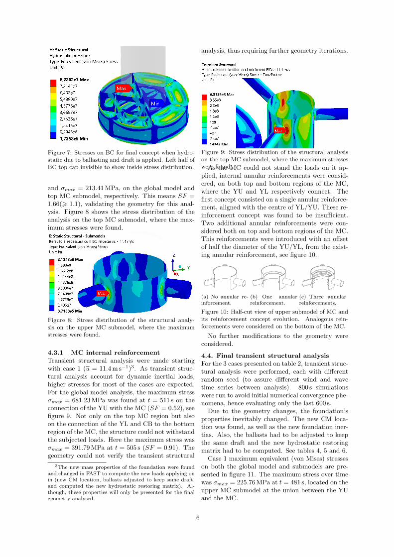
Figure 7: Stresses on BC for final concept when hydro-static due to ballasting and draft is applied. Left half ofBC top cap invisible to show inside stress distribution.

and σmax = 213.41 MPa, on the global model andtop MC submodel, respectively. This means SF =1.66(> 1.1), validating the geometry for this anal-ysis. Figure 8 shows the stress distribution of theanalysis on the top MC submodel, where the max-imum stresses were found.

Figure 8: Stress distribution of the structural analy-sis on the upper MC submodel, where the maximumstresses were found.

4.3.1 MC internal reinforcementTransient structural analysis were made startingwith case 1 (u = 11.4 m s−1)3. As transient struc-tural analysis account for dynamic inertial loads,higher stresses for most of the cases are expected.For the global model analysis, the maximum stressσmax = 681.23 MPa was found at t = 511 s on theconnection of the YU with the MC (SF = 0.52), seefigure 9. Not only on the top MC region but alsoon the connection of the YL and CB to the bottomregion of the MC, the structure could not withstandthe subjected loads. Here the maximum stress wasσmax = 391.79 MPa at t = 505 s (SF = 0.91). Thegeometry could not verify the transient structural

3The new mass properties of the foundation were foundand changed in FAST to compute the new loads applying onin (new CM location, ballasts adjusted to keep same draft,and computed the new hydrostatic restoring matrix). Al-though, these properties will only be presented for the finalgeometry analysed.

analysis, thus requiring further geometry iterations.

Figure 9: Stress distribution of the structural analysison the top MC submodel, where the maximum stresseswere found.As the MC could not stand the loads on it ap-plied, internal annular reinforcements were consid-ered, on both top and bottom regions of the MC,where the YU and YL respectively connect. Thefirst concept consisted on a single annular reinforce-ment, aligned with the centre of YL/YU. These re-inforcement concept was found to be insufficient.Two additional annular reinforcements were con-sidered both on top and bottom regions of the MC.This reinforcements were introduced with an offsetof half the diameter of the YU/YL, from the exist-ing annular reinforcement, see figure 10.

A A

B B

C C

D D

E E

F F

8

8

7

7

6

6

5

5

4

4

3

3

2

2

1

1

DRAWN

CHK'D

APPV'D

MFG

Q.A

UNLESS OTHERWISE SPECIFIED:DIMENSIONS ARE IN MILLIMETERSSURFACE FINISH:TOLERANCES: LINEAR: ANGULAR:

FINISH: DEBURR AND BREAK SHARP EDGES

NAME SIGNATURE DATE

MATERIAL:

DO NOT SCALE DRAWING REVISION

TITLE:

DWG NO.

SCALE:1:100 SHEET 1 OF 1

A3

WEIGHT:

ANSYS_DeepCwind_ExternalSurf_NoRingsMC

(a) No annular re-inforcement.

(b) One annularreinforcement.

(c) Three annularreinforcements.

Figure 10: Half-cut view of upper submodel of MC andits reinforcement concept evolution. Analogous rein-forcements were considered on the bottom of the MC.

No further modifications to the geometry wereconsidered.

4.4. Final transient structural analysisFor the 3 cases presented on table 2, transient struc-tural analysis were performed, each with differentrandom seed (to assure different wind and wavetime series between analysis). 800 s simulationswere run to avoid initial numerical convergence phe-nomena, hence evaluating only the last 600 s.

Due to the geometry changes, the foundation’sproperties inevitably changed. The new CM loca-tion was found, as well as the new foundation iner-tias. Also, the ballasts had to be adjusted to keepthe same draft and the new hydrostatic restoringmatrix had to be computed. See tables 4, 5 and 6.

Case 1 maximum equivalent (von Mises) stresseson both the global model and submodels are pre-sented in figure 11. The maximum stress over timewas σmax = 225.76 MPa at t = 481 s, located on theupper MC submodel at the union between the YUand the MC.

6

Table 4: Foundation’s mass properties considering bal-lasting

Properties Original Final

Steel mass 3.8522E+6 kg 9.1882E+6 kgTotal mass 1.3473E+7 kg 1.3473E+7 kgCM below SWL 13.46 m 12.13 mRoll inertia 6.827E+9 kg m−2 6.836E+9 kg m−2

Pitch inertia 6.827E+9 kg m−2 6.836E+9 kg m−2

Yaw inertia 1.226E+10 kg m−2 1.116E+10 kg m−2

Table 5: Ballasting properties.

Properties Original Final

Height at UC 7.830 m - mHeight at BC 5.048 m 3.196 mTotal mass 9.621E+6 kg 4.285E+6 kg

Table 6: Hydrostatic restoring matrix. Entries notshown are zero.

Properties Original Final

Chidr3,3 3,836E+6 N m−1 3,836E+6 N m−1

Chidr4,4 1,074E+9 N m rad−1 1,702E+9 N m rad−1

Chidr5,5 1,074E+9 N m rad−1 1,702E+9 N m rad−1

0 100 200 300 400 500 600Time (s)

100

200

300

400

Max

imum

Stress(M

Pa)

u = 11 ,4 m/s , H s = 2 ,466 m, T s = 13 ,159 s Global model Submodels

Figure 11: von Mises maximum stresses over time forcase 1, for the global model and submodels.

For case 2, the maximum stress over time σmax =342.86 MPa was also located on the union betweenthe YU and the MC, at t = 169 s. This correspondsto a minimum safety factor over time of 1.035, bel-low the minimum limit of 1.1 stated by the GL stan-dard [1]. For this reason, this geometry is not ca-pable of verifying the normative conditions.

0 100 200 300 400 500 600Time (s)

100

200

300

400

Max

imum

Stress(M

Pa)

u = 18 m/s, Hs = 4, 005 m, Ts = 14, 129 s Global model Submodels

Figure 12: von Mises maximum stresses over time forcase 2, for the global model and submodels.

The analysis for case 3 presented higher max-imum stresses over time, going up to σmax =378.63 MPa at t = 292 s, above the yield stressstated by the GL standard [1], of 355 MPa, whichmeans a minimum safety factor of SF = 0.94 over

time. This stress was located also at the connec-tion of the YU with the MC. The yield region canbe seen in figure 14.

0 100 200 300 400 500 600Time (s)

100

200

300

400

Max

imum

Stress(M

Pa)

u = 24 m/s, Hs = 5, 585 m, Ts = 16, 162 s Global model Submodels

Figure 13: von Mises maximum stresses over time forcase 3, for the global model and submodels.

(a) Global model.

(b) Upper MC submodel.

Figure 14: Stress distribution for time of von Misesmaximum stresses on case 3.

The maximum stresses tend to increase with theincrease of wind speed u, and therefore the increaseof the significant wave height Hs and peak periodTp. The main reason why this happens may bedue to the inertial loads accounted by the transientstructural analysis. The inertial loads may dependmainly on the Hs and Tp, since they have a biggerinfluence on the structure’s acceleration. Although,analysis have to be made for increasing Hs and Tpwhile u is kept constant, to attest this hypothesis.

4.5. Modal analysisDespite the final geometry analysed not being capa-ble of standing the loads, it may be close to accom-plish it with some adjustments. Thus, a free-freemodal analysis was performed of the final founda-tion considered, whose the results may be somehowrepresentative of a geometry that verifies the tran-

7

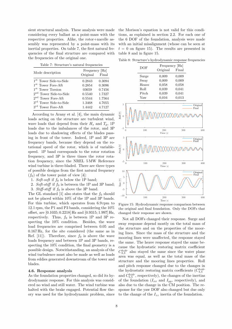
sient structural analysis. These analysis were madeconsidering every ballast as a point-mass with therespective properties. Alike, the rotor+nacelle as-sembly was represented by a point-mass with itsinertial properties. On table 7, the first natural fre-quencies of the final structure are compared withthe frequencies of the original one.

Table 7: Structure’s natural frequencies

Mode descriptionFrequency [Hz]

Original Final

1st Tower Side-to-Side 0.2843 0.30941st Tower Fore-Aft 0.2854 0.30961st Tower Torsion 03659 0.7456

2nd Tower Side-to-Side 0.5540 1.7327

2nd Tower Fore-Aft 0.5544 1.7564

3rd Tower Side-to-Side 1.3468 4.7055

3rd Tower Fore-Aft 1.4442 4.7127

According to Arany et al. [4], the main dynamicloads acting on the structure are turbulent wind,wave loads that depend from their Hs and Tp, 1Ploads due to the imbalances of the rotor, and 3Ploads due to shadowing effects of the blades pass-ing in front of the tower. Indeed, 1P and 3P arefrequency bands, because they depend on the ro-tational speed of the rotor, which is of variable-speed. 1P band corresponds to the rotor rotationfrequency, and 3P is three times the rotor rota-tion frequency, since the NREL 5 MW Referencewind turbine is three-bladed. There are three typesof possible designs from the first natural frequency(f0) of the tower point of view [4]:

1. Soft-soft if f0 is below the 1P band;2. Soft-stiff if f0 is between the 1P and 3P band;3. Stiff-stiff if f0 is above the 3P band.

The GL standard [1] also states that the f0 shouldnot be placed within 10% of the 1P and 3P bands.For this turbine, which operates from 6.9 rpm to12.1 rpm, the P1 and P3 bands, considering the 10%offset, are [0.1035; 0.2218] Hz and [0.9315; 1.997] Hz,respectively. Thus, f0 is between 1P and 3P re-specting the 10% condition. Besides, the waveload frequencies are comprised between 0.05 and0.167 Hz, for the site considered (the same as inRef. [11]). Therefore, since f0 is above the waveloads frequency and between 1P and 3P bands, re-specting the 10% condition, the final geometry is apossible design. Notwithstanding, an analysis of thewind turbulence must also be made as well as loadsfrom eddies generated downstream of the tower andblades.

4.6. Response analysisAs the foundation properties changed, so did its hy-drodynamic response. For this analysis was consid-ered no wind and still water. The wind turbine washalted with the brake engaged. Potential flow the-ory was used for the hydrodynamic problem, since

the Morison’s equation is not valid for this condi-tions, as explained in section 2.2. For each one ofthe 6 DOF of the foundation, analysis were madewith an initial misalignment (whose can be seen att = 0 on figure 15). The results are presented intable 8 and in figure 15.

Table 8: Structure’s hydrodynamic response frequencies

DOFFrequency [Hz]

Original Final

Surge 0,009 0,009Sway 0,009 0,009Heave 0,058 0,058Roll 0,039 0,041Pitch 0,039 0,041Yaw 0,016 0,013

0 100 200 300 400Time (s)

-5

0

5

Roll [

º]

OriginalFinal

0 100 200 300 400

Tempo (s)

-5

0

5

Pitch

[º]

Original

Final

0 100 200 300 400

Tempo (s)

-10

-5

0

5

10

Original

Final

Yaw

[º]

0 100 200 300 400

Tempo (s)

-5

0

5

Roll [

º]

Original

Final

0 100 200 300 400Time (s)

-5

0

5

Pitc

h [º

]

OriginalFinal

0 100 200 300 400

Tempo (s)

-10

-5

0

5

10

Original

Final

Yaw

[º]

0 100 200 300 400Tempo (s)

-5

0

5

Roll [

º]

OriginalFinal

0 100 200 300 400Tempo (s)

-5

0

5

Pitch

[º]

OriginalFinal

0 100 200 300 400Time (s)

-10

-5

0

5

10 OriginalFinal

Yaw

[º]

Figure 15: Hydrodynamic response comparison betweenthe original and final foundation. Only the DOFs thatchanged their response are shown.

Not all DOFs changed their response. Surge andsway response depend mostly on the total mass ofthe structure and on the properties of the moor-ing lines. Since the mass of the structure and themooring lines were unaffected, the response stayedthe same. The heave response stayed the same be-cause the hydrostatic restoring matrix coefficientChidr3,3 also stayed the same since the water planearea was equal, as well as the total mass of thestructure and the mooring lines properties. Rolland pitch response changed due to the changes inthe hydrostatic restoring matrix coefficients (Chidr4,4

and Chidr5,5 , respectively), the changes of the inertiasof the foundation (Ixx and Iyy, respectively), andalso due to the change in the CM position. The re-sponse for the yaw DOF also changed but due onlyto the change of the Izz inertia of the foundation.

8

5 CONCLUSIONS

Due to the incapability of the BCs to stand thehydrostatic pressure, two possible solutions are seenas possible:

1. Internal reinforcement of the BCs, as presentedon this document or with alternative concepts;

2. Replacement of the BC by heave plates, with-out any free interior volume, and thus not tobe affected by the hydrodynamic pressure. Anexample are the heave plates used by the Wind-Float.

The thickness of the overall foundation was foundto be bellow the necessary for the structure to with-stand the existent loads. However, with the increaseof thickness, and the added internal reinforcementson the BC,, the foundation still yield on the unionsof the YU with the MC. This region was consideredto be the weaker region of the entire foundation. Anincrease in the pontoon’s diameter or a reduction ofthe distance between the UC+BC (of the side of thetriangle formed by the columns) may be a possiblesolution to this problem.

The maximum stresses tend to increase with theincrease of wind speed u, and therefore the increaseof the significant wave hight Hs and peak periodTp. This is believed to be because of the inertialloads that may depend mainly on the Hs and Tp,since they have a bigger influence on the structure’smovement. To attest this hypothesis, analysis haveto be made for increasing Hs and Tp while u is keptconstant.

REFERENCES

[1] Rules and Guidelines Industrial ServicesGuideline for the Certification of OffshoreWind Turbines. Standard, Germanischer Lloyd(GL), 2012.

[2] ANSYS. ANSYS advanced analysis techniquesguide. Ansys Help, (November), 2007.

[3] ANSYS. Reduction Techniques, Part 1: Sub-modeling Applicability and Example, 2012.

[4] L. Arany, S. Bhattacharya, J. Macdonald, andS. J. Hogan. Simplified critical mudline bend-ing moment spectra of offshore wind turbinesupport structures. Wind Energy, 2014.

[5] S. Butterfield, W. Musial, and J. Jonkman.Engineering Challenges for Floating OffshoreWind Turbines. 2007.

[6] J. Cruz and M. Atcheson. Floating OffshoreWind Energy: the next generation of wind en-ergy. Spinger, 2016.

[7] M. Hall and A. Goupee. Validation of alumped-mass mooring line model with Deep-Cwind semisubmersible model test data. OceanEngineering, 104, 2015.

[8] M. O. Hansen. Aerodynamics of Wind Tur-bines. 2015.

[9] Wind turbines - Part 3: Design Requirementsfor Offshore Wind Turbines. Standard, Inter-national Electrotechnical Commission (IEC),2006.

[10] J. Jonkman, S. Butterfield, W. Musial, andG. Scott. Definition of a 5-MW reference windturbine for offshore system development. Tech-nical report, NREL, 2009.

[11] J. M. Jonkman. Dynamics modeling and loadsanalysis of an offshore floating wind turbine.Technical report, NREL, 2007.

[12] J. M. Jonkman, T. Larsen, A. C. Hansen,T. Nygaard, K. Maus, M. Karimirad, Z. Gao,T. Moan, I. Fylling, J. Nichols, M. Kohlmeier,J. P. Vergara, D. Merino, W. Shi, and H. Park.Offshore code comparison collaboration withinIEA Wind Task 23: Phase IV results regard-ing floating wind turbine modeling. Technicalreport, NREL, 2010.

[13] J. M. Jonkman, A. N. Robertson, and G. J.Hayman. HydroDyn User’s Guide and TheoryManual HydroDyn User’s Guide and TheoryManual. (March), 2015.

[14] C. Luan, Z. Gao, and T. Moan. Developmentand verification of a time-domain approachfor determining forces and moments in struc-tural components of floaters with an applica-tion to floating wind turbines. Marine Struc-tures, 2016.

[15] E. Madenci and I. Guven. The finite elementmethod and applications in engineering usingANSYS. Spinger, 2006.

[16] P. J. Moriarty and A. C. Hansen. Aerodyntheory manual. Renewable Energy, 2005.

[17] E. Narvydas and N. Puodziuniene. Applica-tions of sub-modeling in structural mechanics.In Mechanika, 2014.

[18] N. Neil Kelley, Bonnie Jonkman. TurbSimUser’s Guide: Version 1.50 TurbSim User’sGuide:. 2009.

[19] A. Robertson, J. Jonkman, and M. Masci-ola. Definition of the Semisubmersible FloatingSystem for Phase II of OC4. Golden, CO, 2014.

9

[20] A. Robertson, J. Jonkman, F. Vorpahl,J. Qvist, and et al. Offshore code compar-ison collaboration, Continuation within IEAwind Task 30: Phase II results regarding afloating semisubmersible wind system. Pro-ceedings of the 33rd International Conferenceon Ocean, Offshore and Arctic Engineering(OMAE2014), 2014.

[21] F. Wendt, A. Robertson, J. Jonkman, andG. Hayman. Verification of New Floating Ca-pabilities in FAST v8. Proceedings of the AIAASciTech, 2015.

10