Page 1
ANALYSIS OF THE TRIBOLOGICAL BEHAVIOR IN TRANSVERSELY ISOTROPIC MATERIALS UTILIZING ANALYTICAL AND FINITE ELEMENT METHODS
by
Xinguo Ning
B.S., Northeastern Institute of Heavy Machinery, 1985
M.S., Huazhong University of Science and Technology, 1988
Submitted to the Graduate Faculty of
School of Engineering in partial fulfillment
of the requirements for the degree of
Doctor of Philosophy
University of Pittsburgh
2002
Page 2
ii
UNIVERSITY OF PITTSBURGH
SCHOOL OF ENGINEERING
This dissertation was presented
by
Xinguo Ning
It was defended on
December 11, 2002
and approved by
Anne M. Robertson
William S. Slaughter
Patrick Smolinski
James H.-C. Wang
Michael R. Lovell Dissertation Director
Page 3
iii
ABSTRACT
ANALYSIS OF THE TRIBOLOGICAL BEHAVIOR IN TRANSVERSELY ISOTROPIC
MATERIALS UTILIZING ANALYTICAL AND FINITE ELEMENT METHODS
Xinguo Ning, PhD
University of Pittsburgh, 2002
This dissertation develops methods for evaluating the tribological behavior of anisotropic
materials. The underlying objectives of the work are: (1) to elucidate the relationship between
the sliding frictional contact and the fiber orientations of FRP composites; (2) to explore the
relationship between the anisotropic strength and the wear of FRP composites and develop an
innovative wear model of FRP composites; and (3) to derive a general approximate solution for
analyzing the contact behavior of transversely isotropic coatings such solid lubricant films.
The first goal was achieved in two steps. First, by incorporating anisotropic contact
theory, the elastic properties of FRP composites, and the analytical expressions of Barnett-Lothe
tensors, the contact behavior of FRP composites in the three principal fiber orientations
(transverse, normal, parallel) was deduced. Specially, the influence of fibers, matrices, volume
fractions, and friction coefficients on the contact behavior was ascertained. Next, through the
numerical solution of the explicit expressions of Barnett-Lothe tensors, the relationship between
the contact performance and the arbitrary fiber orientations was examined. Based on this
approach, the influence of fiber orientations on the contact pressure and the contact patch was
determined.
Page 4
iv
To develop an anisotropic wear model of FRP composites, the Tsai-Wu failure strength
criterion was employed to establish the relationship between the wear and the contact stress. The
theoretically predicated results were in good agreement with the previously published
experimental data. This correlation demonstrates that the anisotropic failure strength criteria may
be used to explain the anisotropy of wear in FRP composites.
Finally, a set of approximate solutions for thin, transversely isotropic coatings was
derived to gain deep insight into the coated structures. These easy-to-use solutions are helpful for
optimizing the contact behavior of thin coatings used in the design of contacting components.
DESCRIPTORS Anisotropic
Coating
Composites
Contact Behavior
Fiber Reinforced Polymer
Friction
Tribology
Wear
Page 5
ii
ACKNOWLEDGMENTS
I am deeply indebted to my advisor, Dr. Michael Lovell for his guidance, support,
collaboration and encouragement throughout my education and research. I also would like to
gratefully thank Dr. William Slaughter for his guidance and collaboration on the mechanics
analysis of this research. I deeply appreciate Dr. James Wang, who not only serves on my
committee but also is generous to give me great help. I am equally indebted to my advisory
committee members, Dr. Patrick Smolinski, and Dr. Anne Robertson, for their providing
invaluable suggestions towards this research.
I gratefully thank Mr. Clint Morrow for his collaboration and discussion about the
content in chapter 5. I am grateful for the support of the Department of Mechanical Engineering
at University of Pittsburgh. My thanks also go to ANSYS Inc. for their offering me the 2001
summer internship. I also thank Mr. Grama Bhashyam, Dr. Guoyu Lin and Dr. Jin Wang at
ANSYS Inc. for their guidance.
Finally, I wish to express my deep appreciation to my dear parents and brother and sisters
for their support, affection and inspiration throughout my education.
Page 6
iii
TABLE OF CONTENTS
ABSTRACT.................................................................................................................................III
ACKNOWLEDGMENTS ........................................................................................................... II
LIST OF TABLES ...................................................................................................................... VI
LIST OF FIGURES ...................................................................................................................VII
NOMENCLATURE.................................................................................................................... IX
1.0 INTRODUCTION....................................................................................................................1
1.1 FRP Composites ....................................................................................................................2
1.1.1 Wear Anisotropy Of FRP Composites............................................................................2
1.1.2 Contact Pressure Of FRP Composites ............................................................................4
1.2 Contact Problems Of Coating Structures...............................................................................5
1.3 Motivations ............................................................................................................................7
1.4 Objectives ..............................................................................................................................8
2.0 ANALYSIS OF TWO-DIMENSIONAL ANISOTROPIC CONTACT .............................9
2.1 Problem Formulation .............................................................................................................9
2.1.1 Elastic Properties Of Composites .................................................................................11
2.1.2 Boundary And Frictional Conditions............................................................................13
2.1.3 Frictional Sliding Contact Pressure ..............................................................................15
3.0 CONTACT PERFORMANCE IN PRINCIPAL FIBER ORIENTATIONS...................17
3.1 Elastic Constants Of Orthotropic Materials.........................................................................17
Page 7
iv
3.2 Components Of Barnett-Lothe Tensors...............................................................................19
3.3 Numerical Results And Discussion .....................................................................................21
3.3.1 Influence Of Fiber Orientations ....................................................................................21
3.3.2 Influence Of Fiber Materials.........................................................................................33
3.3.3 Influence Of Fiber Volume Fractions ...........................................................................37
3.3.4 Influence Of Matrix Materials ......................................................................................42
3.3.5 Influence Of Friction Coefficient..................................................................................47
3.4 Conclusion ...........................................................................................................................51
4.0 CONTACT BEHAVIOR IN ARBITRARY FIBER ORIENTATIONS...........................53
4.1 Off-Axis Elastic Properties Of Composites.........................................................................54
4.2 Explicit Expression Of Barnett-Lothe Tensors....................................................................56
4.3 Solutions And Discussion....................................................................................................59
4.4 Conclusion ...........................................................................................................................68
5.0 DEVELOPMENT OF WEAR MODEL FOR FRP COMPOSITES ................................69
5.1 Wear Analysis......................................................................................................................69
5.2 Anisotropic Strength Approach ...........................................................................................71
5.3 Development Of Wear Model..............................................................................................83
5.4 Comparison With Experimental Data..................................................................................85
5.5 Conclusion ...........................................................................................................................92
6.0 AXISYMMETRIC CONTACT OF A THIN, TRANSVERSELY ISOTROPIC
ELASTIC LAYER...............................................................................................................93
6.1 Problem Formulation ...........................................................................................................94
6.1.1 Governing Equations ....................................................................................................96
Page 8
v
6.1.2 Boundary Conditions ....................................................................................................97
6.2 Approximate Solutions ........................................................................................................99
6.2.1 Unbonded, Frictionless Interface ................................................................................100
6.2.2 Ideally Bonded Interface.............................................................................................104
6.3 Results And Discussion .....................................................................................................107
6.3.1 Reduced Solutions For Isotropic Materials.................................................................107
6.4 Comparison With Finite Element Analysis .......................................................................109
6.4.1 FEM Model.................................................................................................................109
6.4.2 Comparison For Bonded Layer...................................................................................112
6.4.3 Comparison For Unbonded Layer ..............................................................................112
6.5 Conclusion .........................................................................................................................114
7.0 SUMMARY AND FURTHER CONSIDERATION.........................................................115
BIBLIOGRAPHY......................................................................................................................118
Page 9
vi
LIST OF TABLES
Table 1 Material properties of Epoxy/T300 FRP composite ........................................................ 24
Table 2 Material Properties........................................................................................................... 32
Table 3 Material properties of PEEK/AS4 graphite FRP ............................................................. 43
Table 4 Strength of FRP composites ............................................................................................ 78
Table 5 Material strength of T300/Epoxy FRP composites.......................................................... 91
Table 6 Verification of the predicted data for T300/Epoxy.......................................................... 91
Page 10
vii
LIST OF FIGURES
Figure 1 Contact model of a rigid cylinder on FRP composites................................................... 10
Figure 2 Principal fiber orientations and the sliding direction ..................................................... 18
Figure 3 Pressure for Epoxy/T300 in three principal fiber direcitons .......................................... 23
Figure 4 Finite element model of a cylinder on composites......................................................... 26
Figure 5 Finely meshed contact surface in x-y plane ................................................................... 27
Figure 6 Comparison of analytical and numerical solutions ........................................................ 29
Figure 7 Pressure in transverse orientation for different fibers .................................................... 34
Figure 8 Pressure in normal orientation for different fibers ........................................................ 35
Figure 9 Pressure in parallel orientation for different fibers......................................................... 36
Figure 10 Pressure in transverse orientation for different fiber fractions .................................... 39
Figure 11 Pressure in normal orientation for different fiber fractions.......................................... 40
Figure 12 Pressure in parallel orientation for different fiber fractions ........................................ 41
Figure 13 Pressure in transverse orientation for different matrices ............................................. 44
Figure 14 Pressure in normal orientation for different matrices................................................... 45
Figure 15 Pressure in parallel orientation for different matrices .................................................. 46
Figure 16 Pressure in TL for different friction coefficients.......................................................... 48
Figure 17 Pressure in NL for different friction coefficients ......................................................... 49
Figure 18 Pressure in PL for different friction coefficients.......................................................... 50
Page 11
viii
Figure 19 Transition of fiber orientations from TL (θ=0deg) to NL (θ=90deg) .......................... 55
Figure 20 Variation of the maximum pressure Pmax with the fiber orientation............................. 61
Figure 21 Variation of δ with the fiber orientation....................................................................... 63
Figure 22 Variation of contact patch width with the fiber orientation ......................................... 65
Figure 23 Ellipsoidal failure stress envelope for Glass/Epoxy: x, y –longitudinal, transverse
principal stresses, respectively; z-shear stress .............................................................. 75
Figure 24 Biaxial stresses (a) off-axis uniaxial loading; (b) off-axis biaxial loading .................. 76
Figure 25 Failure compressive stress xσ vs. fiber orientation from PL/TL to NL........................ 79
Figure 26 Compressive stress xσ vs. fiber orientation from PL/TL to NL for T300/Epoxy ........ 82
Figure 27 Schematic model of plane stress................................................................................... 86
Figure 28 Theoretical wear trend for T300/Epoxy from PL/TL (0deg) to NL (90deg) ............... 88
Figure 29 Verification of the results from TL (0deg) to NL (90deg) ........................................... 90
Figure 30 Geometry of the contacting surfaces ............................................................................ 95
Figure 31Comparison between the predicated maximum contact pressure p(0) and the FEM
results .......................................................................................................................... 111
Figure 32 Contact pressure for the bonded and unbonded cases ................................................ 113
Page 12
ix
NOMENCLATURE
a left width of the contact patch
A transformation matrix
b right width of the contact patch
c elastic constant
C compliance matrix
e$ orthonormal vector basis
E Young's modulus
f friction coefficient or subscript represents fiber
F applied normal force
G shear modulus
H material hardness
i subscript, i=1…6
j subscript, j=1…6
k wear factor
K bulk modulus
L Barnett-Lothe tensor
m subscripts expressing the resin
p(x) pressure distribution
Page 13
x
r radius of curvature of the parabolic cylinder
R matrix
S Barnett-Lothe tensor
Ss shear strength
t layer thickness and subscript represents transverse or tensile
T matrix
u displacement
v sliding direction
V volume fractions
w& wear rate
Xc compressive strength in X-axis
Xt tensile strength in X-axis
y(x) indenter profile
Y yield stress
Yc compressive strength in Y-axis
Yt tensile strength in Y-axis
α parameter
β characteristic parameter
ν Poisson’s ratios
iσ normal stress components
iε normal strain components
ijτ shear stress components
η parameter
Page 14
xi
δ characteristic parameter
ijγ shear strain components
ξ sin(θ)
ζ cos(θ)
ρ parameter
λ parameter
Page 15
1
1.0 INTRODUCTION
The word tribology, derived from the Greek word tribos meaning rubbing, first appeared
in Jost’s report [1] and was defined as: ‘… The science and technology of interacting surfaces in
relative motion and the practices related thereto.’ As interdisciplinary science and technology, it
includes friction, wear and lubrication.
Tribology is crucial to modern industry. Many tribological components such as brakes,
clutches, driving wheels, bolts, nuts, gears, cams, bearings, and seals are applied in the
machinery. The friction and wear appearing in these operations is one of the largest energy
losses. It was estimated in 1966 [1] that the United Kingdom could save approximately 500
million pounds per year, and the United States could save in excess of 16 billion dollars per year
by better tribological designs. Therefore, research in tribology may lead to substantially
economical saving and better performance of machines.
The commonly used materials in tribological components range from metals, alloys to
ceramics, solid lubricants, polymers, and composites. Among these materials, several are
transversely isotropic in nature such as unidirectional continuous fiber-reinforced polymer (FRP)
composites, and molybdenum disulphide (MoS2). The former material is a class of tribological
materials that possess unique self-lubricating capability and low noise, and the latter one
represents an important solid lubricant that may be coated on the surfaces of tribological
components to meet the severe work conditions and often reduce the cost. FRP composites and
coated structures are widely utilized in tribological components such as gears, seals, and
bearings, and hence have been theoretically and experimentally studied.
Page 16
2
1.1 FRP Composites
FRP composite materials are comprised of matrix and fiber elements. The fibers of FRP
composites give them their unique mechanical characteristics. The most common filled fiber
reinforcements are glass, carbon (graphite), and aramid (Kevlar 49). E-glass fibers are created
using a calcium aluminoborosilicate formulation that produces beneficial mechanical properties
at very reasonable cost. Carbon or graphite fibers are currently the best known and most widely
utilized high performance composite. Aramid is a class of aromatic–polyamide fibers that are
produced using para-phenylene terephthalamide. The purpose of the FRP composite matrix
material is to bind the fibers together. By virtue of their cohesive and adhesive characteristics,
the resins give FRP materials the ability to transfer load to and between fibers, and to protect
them from environmental conditions and handling. The most common matrix materials are
epoxy, PEEK (polyether ether keton), and PPS (polyphenylene sulfide).
With numerous possible material combinations, FRP composites provide nearly
unlimited possibilities for optimizing the tribological performance of mating components. For
this reason, polymer composites are widely utilized in numerous applications including seals,
bearings, gears, and artificial prosthetic joints.
1.1.1 Wear Anisotropy Of FRP Composites
Unidirectional continuous fiber-reinforced polymer composites exhibit significant
tribological anisotropy due to their heterogeneity. As described in the literature [2-6], fiber
orientations have a significant influence on the wear and friction behavior of FRP composites.
Page 17
3
Experimental investigation has shown that the largest wear resistance in FRP composites
occurred when the sliding was normal to the fiber orientation, while the lowest wear resistance
occurred when the fiber orientation was in the transverse direction. Experiments have also shown
that the coefficient of friction and the wear in FRP composites depend on several factors
including the material combination, the fiber orientation, and the surface roughness. Sung and
Suh [2] tested T300/epoxy and Kevlar 49/epoxy composites and explained the wear phenomena
using a delamination theory. In their work, the wear was found to be related to the stress field
under the indentation of an asperity, the mechanics of the crack nucleation and propagation, and
the material properties.
Tsukizoe and Ohmae [7] later performed numerous experiments to establish the influence
of fiber orientation, elastic modulus, loading condition, friction coefficient, interlaminar shear
strength, and the fracture strain on the wear rate of FRP composites. Based on the experimental
results, they proposed the following empirical wear rate equation:
1
s
fpwE I
λ
ρ =
& (1.1)
where ρ is the wear constant; λ is an exponential parameter; f is the friction coefficient; p is the
applied pressure; E is the elastic modulus and Is is the interlaminar shear strength. By means of
the above empirical wear equation, Lhymn [3] investigated the tribological properties of
unidirectional polyphenylene sulfide-carbon fiber laminate composites. He attempted to
qualitatively explain the effect of fiber orientation in terms of the difference in the interlaminar
shear strength and the fracture strain of the three principal fiber orientations. In order to
theoretically elucidate the effect of fiber orientation on the wear of composites, Ovaert and Wu
Page 18
4
[8, 9] constructed a relationship between the wear rate of normally oriented FRP composites and
the fiber debonding depth under the indentation of a spherical asperity. For the wear of FRP
composites in the parallel-oriented fiber orientation, Ovaert [10, 11] later introduced a model of a
beam lying on a foundation to simulate the fibers in a polymer matrix. These models clearly
demonstrate the wear modes in the three principal directions and the influence of the
microstructures of FRP composites on the wear.
1.1.2 Contact Pressure Of FRP Composites
The classical Hertzian contact theory cannot be applied to anisotropic materials such as
FRP composites, so several researchers have analyzed the contact between anisotropic bodies.
Klingworth and Stronge [12] analyzed a plane punch indentation of anisotropic elastic half space
with the potential function approach. Fan and Keer [13] derived a general solution for two-
dimensional contact on anisotropic half-space by combining the approach of analytical
continuation [14] and Stroh’s formalism [15]. This method can be used to evaluate the in-plane
deformation and the coupled deformation between the in-plane and the anti-plane. Fan and Hwu
[16-18] studied general contact problems for an anisotropic elastic half-plane and obtained the
closed-form solutions for the sliding contact of bodies on anisotropic elastic planes. Recently,
Ning and Lovell [19, 20] revealed the contact behavior for arbitrary fiber orientations of
unidirectional continuous FRP composites and highlighted the correlation between the contact
characteristics and the wear.
Page 19
5
1.2 Contact Problems Of Coating Structures
Surface coatings have become widely utilized in the engineering community due to the
many potential benefits they offer. These coatings, which may be isotropic or anisotropic in
nature, are typically used to enhance the contact characteristics and improve the tribological
performance of mating components. One of the most common applications for surface coatings
is in rolling element or slider bearings that operate in vacuum or low temperature environments.
As described in the literature [cf. 21], oils and other liquid lubricants may evaporate in vacuum
and contaminate instrumentation. At low temperature, fluid lubricant viscosity dramatically
increases and may become insufficient over time. In such applications, solids lubricant coatings
are often the most effective method of reducing wear in contacting components. Coatings are
generally very thin layers of soft metals (e.g. Au, Ag, In, and Pb), laminar solids (e.g., MoS2 and
Boron Nitride), or polymers (e.g., PTFE, Polyamide composites and Phenolic and Epoxy), which
are deposited onto a substrate surface.
When solid lubricant coatings are applied to a substrate, the contact stress and
displacement fields significantly deviate from the Hertzian contact profile within the half-space.
This causes significant problems to designers because there are no closed-form solutions
available for analyzing three-dimensional coated surface contact for even simple geometries.
Reviewing the literature, various researchers have analytically investigated axi-symmetrical
contact problems with isotropic elastic layers. Sneddon [22] expressed the axi-symmetrical
punch stress and displacement in the layer in terms of Hankel integral transforms. Chen [23], and
Chen and Engel [24] studied multi-layered media by respectively employing the Fourier integral
transform and the least square integral approach. Matthewson [25] approximated the stress
Page 20
6
within thin compliant layers by averaging through the layer thickness. Aleksandrov [26]
obtained asymptotic solutions for the stresses in a layer and Jaffar [27] gave a numerical solution
for the contact traction and displacement by using modified Legendre polynomials. O’Sullivan
and King [28] analyzed sliding contact of a sphere on an elastic layered half-space and
determined the stress fields using the Papkovich-Neuber potentials. Johnson [29] developed an
approximate method based on the assumption that “ plane sections remain plane after
compression”, and analyzed frictionless cylinder indenting an unbonded or bonded layer on a
rigid foundation. His solution was found to be in good agreement with Meijers’ [30] when the
ratio of contact semi-width to layer thickness is large. Jaffer [31] later employed Johnson’s
assumption to obtain an asymptotic solution for the axi-symmetrical indentation of a thin elastic
layer bonded or unbonded to a rigid foundation. Barber [32] extended the same assumption to
general three-dimensional isotropic elastic thin layer punch problems with arbitrary shaped
indenters. Tian and Bhushan [33] analyzed the contact of 3-dimensional layered with rough
surfaces by variational principle.
Anisotropic coatings demonstrate more complicated contact characteristics than isotropic
elastic layers because of their directional dependence. Ovaert [34] analyzed the punch problem
of a rigid ellipsoidal indenter on a transversely isotropic solid lubrication film. Kuo and Keer
[35] obtained numerical solutions for transversely isotropic multi-layered media by means of
Hankel transforms. Lovell et al. [21, 36, 37] used finite element method to investigate the normal
stress and tangential friction characteristics of an elastic sphere in contact with transversely
isotropic, coated elastic substrate surface.
Page 21
7
1.3 Motivations
For the purpose of fully utilizing the beneficial tribological characteristics of FRP
composites, it is necessary to obtain an in-depth knowledge of their contact behavior and
establish the relationship between the wear and the fiber orientations. However, Hertzian and
other fundamental contact theories are not valid for FRP composites due to their anisotropy. The
present investigation will incorporate the analytical and the explicit expressions of Barnett-Lothe
tensors [38, 39] to the analytical solutions to reveal the effect of fiber orientations on the contact
behavior and to develop an anisotropic wear model of unidirectional continuous FRP
composites.
As reviewed earlier in the chapter, there has not existed an exact closed-form solution for
the analysis of the transversely isotropic, layered system. However, a set of approximate
analytical solutions may provide not only a convenient design tool to predicate the performance
of coating systems but in-depth understanding of the roles of the material properties as well. In
this work, approximate solutions will be derived based on specified assumptions.
Page 22
8
1.4 Objectives
The present research has two main goals; one is to attempt to elucidate how the fiber
orientation affects the wear of unidirectional continuous FRP composites and to model the
anisotropic wear, the other is to derive approximate formulae for a thin, transversely isotropic
coatings bonded or unbonded on a rigid foundation. To achieve the first goal, there are two steps:
• Propose an analytical approach to investigate the two-dimensional contact behavior of
FRP composites, including the effect of fiber orientations, fiber and matrix materials,
friction coefficients, and material volume fractions
• Based on anisotropic strength criteria, develop anisotropic wear model for FRP
composites
To achieve the second goal, the Johnson’s assumption [29] was incorporated in the basic
elastic theory.
Page 23
9
2.0 ANALYSIS OF TWO-DIMENSIONAL ANISOTROPIC CONTACT
2.1 Problem Formulation
In the present investigation, the unidirectional continuous FRP composites will be
modeled as a quasi-homogeneous, transversely isotropic elastic half-space that is in contact with
an infinitely long, rigid parabolic cylinder. A Cartesian coordinate system will be defined such
that the Y-axis coincides with the vertical axis of the cylinder, as shown in Fig. 1. The sliding
direction, v, is perpendicular to the axis of cylinder, and motion occurs from left to right. (- a ,b )
is the interval of the contact patch,
Page 24
10
Figure 1 Contact model of a rigid cylinder on FRP composites
Y
v
X
a b
Composites
Page 25
11
2.1.1 Elastic Properties Of Composites
When the coordinates coincide with the principal axes of the elastic half-plane (as in
Fig.1), the stress/strain relationship of uni-directional composites can be sufficiently described
using five elastic constants. In such a condition the X-Y plane is considered transversely
isotropic, and the generalized Hooke’s law becomes:
11 12 131 1
12 11 132 2
13 13 333 3
4423 23
4431 31
6612 12
0 0 00 0 00 0 0
0 0 0 0 00 0 0 0 00 0 0 0 0
c c cc c cc c c
cc
c
σ εσ εσ ετ γτ γτ γ
=
(2.1)
where cij are the components of material stiffness matrix C, and c66=(c11-c12)/2; iσ and iε are the
normal stress and strain components; and ijτ and ijγ are the shear stress and strain components,
respectively. The components of the stiffness matrix may be expressed in terms of engineering
constants:
23 3211 22
2 3
1c cE Eν ν−
= =∆
(2.2)
21 31 23 23 32 1312
2 3 1 3
cE E E E
ν ν ν ν ν ν+ += =
∆ ∆ (2.3)
31 21 32 13 12 2313 23
2 3 1 3
c cE E E E
ν ν ν ν ν ν+ += = =
∆ ∆ (2.4)
Page 26
12
12 2133
1 3
1cE Eν ν−
=∆
(2.5)
44 55 23 31c c G G= = = (2.6)
66 12c G= (2.7)
where 12 21 23 32 13 31 21 32 13 1 2 3(1 2 ) / E E Eν ν ν ν ν ν ν ν ν∆ = − − − − ; E1 (=E2) is the elastic modulus in the
plane of transverse isotropy; E3 is the longitudinal elastic modulus normal to the plane of
isotropy; ν31 is the longitudinal Poisson’s ratio and ν12 is the transverse Poisson’s ratio; and G31
and G12 are the transverse and the longitudinal shear moduli, respectively.
Unlike those of metals, the elastic constants of FRP composites exhibit the mixed
properties of the constituents. If the fiber is assumed to be isotropic, the elastic constants can be
determined using the representative elastic properties of the fiber and the matrix, as presented by
Rosen [40] and Hashin [41]:
2
3
4 ( )/ / 1/
m f f mm m f f
m f f m m
V VE E V E V
V k V k Gν ν−
= + ++ +
(2.8)
31
( )(1/ 1/ )/ / 1/
m f f m m fm m f f
m f f m m
V V k kV V
V k V k Gν ν
ν ν ν− −
= + ++ +
(2.9)
3 2 2
12 3 2 2
( )(1 ) 3( )(1 ) 3
m f f f m mm
f f f m m
V V V VG G
V V V Vα β ρ βα ρ β+ + −
=− + −
(2.10)
121 2 2
12 31 3
4(1 4 / )
t
t t
k GE Ek G k Eν
= =+ +
(2.11)
12 1 12/ 2 1E Gν = − (2.12)
Page 27
13
, ( i, j 1, 2, 3 )ji
ij ji
EEν ν
= = (2.13)
31
(1 )(1 )
m m f fm
m f f m
V G V GG G
V G V G+ +
=+ +
(2.14)
( )m f f f m m mt
m f f m m
k k V k V k Gk
V k V k G+ +
=+ +
(2.15)
( ) ( 1)mα γ β γ= + − (2.16)
2 22(1 2 ), 2(1 2 )f f f f m m m mk E k Eν ν ν ν= − − = − − (2.17)
1 (3 4 ), 1 (3 4 ), m m f fβ ν β ν= − = − (2.18)
( ) (1 ), m f f f mG Gρ β γβ γβ γ= − + = (2.19)
where k is the bulk modulus; V is the volume fraction of the fiber or the matrix; and the
subscripts f, m, and t respectively express the fiber, matrix, and transverse.
2.1.2 Boundary And Frictional Conditions
In the case of two-dimensional sliding contact, the boundary conditions on the
anisotropic half-plane are given by:
12 22 , -f a x bτ σ= ≤ ≤ (2.20)
12 22 0, or x a x bτ σ= = < − > (2.21)
2
, - 2xy(x)= a x br
≤ ≤ (2.22)
Page 28
14
where 12τ is the shear stress component on the contact plane in the sliding direction, 22σ is the
normal stress component on the contact plane, y(x) is the mathematical expression of the profile
of the indenter, and r is the radius of the curvature of the parabolic cylinder,. In Eqs. 2.20-2.22, (-
a ,b ) is the interval of the contact patch, and f is the friction coefficient of the composite in the
direction of the X-axis.
Since the problem analyzed in this work assumes steady sliding motion, a dynamic
coefficient of friction will be used for f. The composites’ frictional coefficients may be
calculated using the law of mixtures [7] if the dependence of the frictional coefficient on the
reinforcement orientation is negligible:
1( )f f m mf V f V f −= + (2.23)
In this work, it is assumed that the dependence of the frictional coefficient on the
reinforcement orientation might be negligible. It is noted that the friction coefficient varies with
the fiber orientation as shown in the previous experimental results [2]. In order to obtain a
theoretical solution for the effect of material anisotropy, however, the friction coefficient of
composites was assumed to be constant. This is of course a simplification to a more complex
phenomenon, but is required for the purpose of obtaining useful analytical results.
Page 29
15
2.1.3 Frictional Sliding Contact Pressure
The two-dimensional sliding contact pressure on the anisotropic elastic half-plane may be
derived using analytical continuation method [14] and Stroh’s formalism [15]. In this case, the
following closed-form solutions have been obtained by Hwu and Fan [17]:
12sin( )( ) ( ) ( )( )
p x b x x ar
δ δδπβ β
−= − ++
(2.24)
1 arg( ) ,2
βδπ β
= − 0 1δ≤ ≤ (2.25)
2 ( )(1 )
rFa δ β βπ δ
+=
− (2.26)
2 (1 )( )rFb δ β βδπ
− += (2.27)
where F is the normal applied load, β is a parameter that reflects the anisotropic elastic
properties of materials, β is the conjugate of β, and δ is a parameter to characterize the
symmetry of the contact patch with respect to the Y-axis.
Equations 2.24-2.27 describe a two-dimensional contact of a parabolic cylinder on
general anisotropic elastic half-plane. The contact pressure distribution is characterized by the
parameters of β and δ. The value of β is determined by Barnett-Lothe tensors.
* *22 21M fMβ = + (2.28)
Page 30
16
where *ijM is the components of the Hermitian matrix, given by:
* 1( )M I iS L−= − (2.29)
where I is a unit matrix. L and S are two of three Barnett-Lothe tensors. So the analysis of
contact performance involves the determination of the Barnett-Lothe tensors. They appear in the
Stroh’s formalism of two- or three- dimensional deformations of anisotropic elastic materials.
Physically, L (except L33) represents a uniform stress state in an anisotropic elastic solid, and S is
related to the strain components [42]. Mathematically, they have different definitions shown in
their explicit expressions for generally anisotropic materials.
The values or the expressions of the Barnett-Lothe tensors depend upon the anisotropy of
materials. Firstly, the orthotropic materials are discussed. And then generally anisotropic
materials are evaluated for the arbitrary fiber orientations.
Page 31
17
3.0 CONTACT PERFORMANCE IN PRINCIPAL FIBER ORIENTATIONS
3.1 Elastic Constants Of Orthotropic Materials
If the cylinder slides along the principal fiber orientations, the coordinate axes coincide
with the principal axes of the elastic half-space (as in Fig.1). In this case, the material is
orthotropic, and the stress and strain of the in-plane and the anti-plane can be decoupled. For
example, for the TL orientation, the generalized Hooke’s law is simplified as:
1 11 12 1
2 12 11 2
12 66 12
00
0 0
c cc c
c
σ εσ ετ γ
=
(3.1)
The stress/strain relations corresponding to the sliding contact directions of NL, and PL
can be similarly given. As shown in Fig. 2, three different fiber orientations will be considered:
(1) the transverse fiber orientation (TL), (2) the normal orientation (NL), and (3) the parallel
fiber orientation (PL).
Page 32
18
Figure 2 Principal fiber orientations and the sliding direction
matrix
fiber
NL
TL
PL
Page 33
19
3.2 Components Of Barnett-Lothe Tensors
For the contact of two orthotropic elastic bodies, the explicit expression of β is [17]:
(1) (2) (1) (2) (2) (1)22 22 12 22 12 22(1) (2)
22 22
1 ( )L L if S L S LL L
β = + + − (3.2)
where Lij and Sij are the components of Barnett-Lothe tensors, L and S. Superscripts represent the
elastic bodies.
If a rigid body slides on orthotropic materials, the value of (1)22L is infinite, so the value of
β reduces to [17]:
12
22 22
1 SifL L
β = − (3.3)
L and S are two of three Barnett-Lothe tensors. The analytical expressions of L and S for
orthotropic materials have been given in terms of elastic constants cij by Dongye and Ting [38].
The non-zero components of the Barnett-Lothe tensors for orthotropic materials are as follows
[17]:
21
2211661222
1222116621 )2(
)(
++
−=
ccccccccc
S (3.4)
21112212 SccS −= (3.5)
2122111211 )( ScccL += (3.6)
Page 34
20
11112222 LccL = (3.7)
21)( 554433 ccL = (3.8)
It is important to note that the parameters of β and δ reflect the degree of anisotropy
properties and the amount of friction. For smooth surface, the value of δ is 0.5 and the contact
profile is symmetrical about the vertical axis of the parabolic cylinder. For surfaces with friction,
the contact patch becomes asymmetrical. The value of δ describes the deviation of the maximum
contact pressure from the axis of the parabolic cylinder. If the value of δ is less than 0.5, the
maximum normal pressure deviates to the side of the moving direction. If δ is larger than 0.5, the
maximum normal pressure would deviate in the opposite direction. Usually, the value of δ is less
than 0.5, and hence the absolute value of b is larger than that of a in the contact patch.
Page 35
21
3.3 Numerical Results And Discussion
Based on the representation of the elastic properties of FRP composites (Eq. 3.1), the
mixture law of friction (Eq. 2.23), and the analytical solutions (Eqs. 2.24-2.27), the influence of
the material combinations, the fiber orientations and the frictional coefficients on the pressure
distributions of FRP composites in three principal alignments can be assessed. In this work, a
normal force of 30 N and an indenter radius of 8 mm will be evaluated.
The pressure distributions for a wide range of contact conditions are investigated and
plotted in figures. In the figures, the horizontal coordinate is marked according to the fraction of
the average contact half-width, x0.
2)( 110 bax += (3.9)
In Eq. 3.9, (- 1a , 1b ) represents the minimum interval of the contact patch. The vertical
coordinate of figures shows the pressure values. From the figures, the variation of the pressure
distribution and the contact area can be determined as a function of the fiber materials, the
volume fractions, the fiber orientations, the resin materials and the friction coefficient.
3.3.1 Influence Of Fiber Orientations
The influence of the fiber orientation on the two-dimensional contact pressure
distribution is illustrated in Fig. 3 for one of the most common FRP composites, epoxy/T300 (see
Page 36
22
Table 1). Examining Fig. 3, it is found that the pressure distribution and the contact patch can
distinctly vary with the principal fiber orientation. In the figure, the smallest maximum pressure
and the largest half-width are obtained when the sliding contact occurs in the transverse (TL)
fiber alignment, while the largest maximum pressure and the smallest half-width occur in the
normal (NL) fiber orientation. The maximum pressure in the NL orientation is actually more
than 300% greater than that of the TL orientation. This can best be explained by investigating the
stiffness variability of FRP composites in different orientations. While in the NL fiber
orientation, the fibers will carry a significant portion of the normal force as the fibers are axially
compressed by the rigid cylinder. This is in contrast to the TL and PL orientations where the
fibers experience a predominantly shearing action and the matrix carries the largest portion of the
normal load. Examining the material properties of epoxy/T300 FRP given in Table 1, it is found
that the fiber is more than 600 times stiffer than the matrix material. Hence, the NL orientation
will be far less compliant than the PL and TL orientations, as illustrated in Fig. 3.
Page 37
23
Figure 3 Pressure for Epoxy/T300 in three principal fiber direcitons
0
50
100
150
-1.5 -1 -0.5 0 0.5 1 1.5x/x0
p(x)(MPa)
TLNLPL
Page 38
24
In Figure 3 it is also found that the maximum pressure in the PL orientation is slightly
larger than that of TL orientation, and that the contact patch in the PL direction is slightly
narrower than the TL direction. This difference between the PL and TL directions can be
attributed to the contribution of the elastic constant C11. The maximum contact pressure is known
to increase with C11. Since C11 in the PL orientation is 30 times larger than that of the TL
orientation, it is natural for the PL orientation to have a greater pressure distribution and a
smaller contact area. It is somewhat surprising, however, that the maximum contact pressure in
Fig. 3 does not vary to a greater extent between PL and TL. Such a finding can be attributed to
the complex compliance behavior of anisotropic materials.
Table 1 Material properties of Epoxy/T300 FRP composite
FRP Fiber Matrix Composites
Modulus
(GPa)
Poisson’s
Ratio
Modulus
(GPa)
Poisson’s
Ratio
Frictional
Coefficient
Epoxy
+
T300
(Carbon fiber)
[2] 228 0.2 0.33 0.34 0.2
Another important set of information provided by Fig. 3 is the influence of fiber
orientation on the symmetry of the contact patch. As shown in the figure and as calculated by Eq.
2.25, the value of δ in the normal fiber orientation is 0.4663. This is the smallest among three
Page 39
25
principal fiber orientations, which indicates the maximum contact pressure in the NL alignment
deviates the farthest distance from the vertical axis of the cylinder. The value of δ in the parallel
(PL) fiber alignment is the highest at 0.4964, which shows that the maximum contact pressure is
the nearest to the vertical axis of the cylinder. Such a finding can again be explained by the fact
that the NL orientation is very stiff, and therefore has a small contact area than the other
orientations. This smaller contact area is more sensitive to deviations caused by friction and
anisotropy, thus leading to small δ values.
Page 40
26
Figure 4 Finite element model of a cylinder on composites
Page 41
27
Figure 5 Finely meshed contact surface in x-y plane
Page 42
28
Before these analytical solution results are related to the published experimental results,
the analytical solution presented in this work will be initially evaluated with respect to results
obtained from the finite element method. For the purpose of assessment, a three-dimensional
finite element model was constructed to simulate a cylinder that slides with respect to a
unidirectional continuous composite substrate. As illustrated in Fig.4, the model is generated
using ANSYS®/LS-DYNA 5.7 and given boundary conditions to obtain results under the
idealized condition of an infinitely long rigid cylinder that is in normal and tangential contact
with a transversely isotropic half-plane. In the model, the half-plane was defined with material
properties of Epoxy/T300 (density is 1536kg/m^3 and the cylinder was specified as a rigid. The
half-plane was defined with dimension of 0.02m wide, 0.05m high, and 0.02m long and its
displacement along the bottom surface were constrained in all three principal directions. The
radius and length of the cylinder are 8 mm and 22 mm, respectively. Both the cylinder and half-
plane were meshed using eight-node structural solid elements and the entire model consisted of
14320 elements for the fiber reinforced polymer composites and 3120 elements for the rigid
cylinder. Finite element results were obtained in PL, TL, and NL orientations by varying the
anisotropic material properties of the half-plane (see Table 2) and then applying normal load
(1N/mm) and a sliding velocity (v=0.1 m/s) to the cylinder.
Page 43
29
Figure 6 Comparison of analytical and numerical solutions
0
5
10
15
20
25
30
1 2 3TL PL NL
P max
(MPa
)
analyticalFEM
Page 44
30
Comparing the analytical and numerical results, good correlation was found in all three
fiber orientations. As illustrated in Fig.6, the differences in the maximum contact pressure
predicted analytically and by the FEM are very small. In fact, the pressures vary by only 0.1
percent and 1.8 percent respectively in the TL and PL orientations. The largest difference
between values is in the NL direction where the analytical and FEM results differ by 6.25
percent. The authors believe that this difference was due to approximations in the numerical
model, and better correlation could have obtained by further refining the mesh of the half-plane
in the contact region. Nonetheless, the small differences between the analytical and FEM results
in all of the directions indicate that the present approach is valid for predicting the contact
behavior of FRP composites.
In the literature, experimental research [2, 7] has indicated that the greatest wear
resistance of FRP composites was obtained when the fiber alignment was normal to the sliding
contact plane (normal orientation), and the lowest wear resistance occurred when the indenter
crossed the fiber alignment (TL). These trends are similarly found using Hwu and Fan’s solution
and can be explained by combining asperity wear rate theory with the results of Fig. 3. In wear
rate models of an asperity’s indentation [8, 9], the wear rate has been shown to be directly
proportional to the contact penetration and inversely proportional to the contact width. In
addition to depicting the influence of fiber orientation on surface pressure, Fig. 3 can also be
utilized to illustrate how the fiber orientation affects the wear in FRP composites. Prior research
[7] has shown that FRP composites have three distinct wear mechanisms: (1) excess thinning of
fibers, (2) fracture of fibers, and (3) peeling of fibers from the matrix. Under large penetrations,
it is more likely for asperities to break fibers and peel them from the matrix. Since the
Page 45
31
penetration is proportional to the size of the contact width, Fig. 3 shows that the cylinder
produces the largest penetration in the transverse fiber orientation and the smallest in the normal
fiber orientation. Therefore Eqs. 2.24-2.27 predict that the largest wear resistance occurs in the
normal fiber orientation and the smallest resistance is obtained in the transverse fiber orientation,
which is identical to the experimental results in [2, 7]. This correlation with the experimental
results shows that the anisotropic theoretical approach utilized in this work may be used to gain
information about the wear of FRP composites.
Page 46
32
Table 2 Material Properties
Fiber Matrix
FRP Modulus
(GPa)
Poisson’s
Ratio
Frictional
Coefficient
Modulus
(GPa)
Poisson’s
Ratio
Frictional
Coefficient
Epoxy
+
Glass Fiber
[8]
72 0.2 0.43
Epoxy
+
Aramid
Fiber
[7]
130 130 0.17
Epoxy
+
Stainless
steel
[7]
186 0.3 0.18
Epoxy
+
AS4
(Carbon
fiber)
[2]
235 0.2 0.2
0.33 0.34 0.3
Page 47
33
3.3.2 Influence Of Fiber Materials
With a large number of fiber materials available, it is important to establish how fiber
material affects the contact behavior of FRP composites. Figs. 7-9 illustrate the variation of the
pressure distributions of four different fiber materials in the transverse, normal and parallel fiber
alignments, respectively. The fiber materials and their properties are given in Table 2. It is
important to note that the polymer resin material was identical for all results in Fig. 7. Examining
the figures, it is found that the variation of the fiber materials has little effect on the profile and
magnitude of the pressure in the PL and TL directions. In the PL results of Fig. 9, it is found that
the maximum normal pressure increases slightly from 43.9825 to 44.7381 MPa for the glass and
carbon fibers respectively. For these fiber materials the value of δ increases from 0.489 to 0.4976
in the PL orientation, showing that the contact profile becomes more symmetric and decreases in
magnitude (see Fig. 9) with increasing fiber elastic modulus.
Turning our attention to the transverse fiber orientation results in Fig. 7, it is similarly
found that the fiber material has little influence on the contact profile. In fact, the contact
pressure only increases from 40.86 MPa for the glass fiber to 41.3 MPa for carbon fiber, and
there is negligible change in the area of the contact patch. There is however, a moderate increase
in the symmetry in the contact patch between glass and carbon fibers, as δ was found to increase
from 0.4569 to 0.4838.
Page 48
34
Figure 7 Pressure in transverse orientation for different fibers
0
10
20
30
40
50
-1.5 -1 -0.5 0 0.5 1 1.5x/x0
p(x)(MPa)GFRPAFRPSFRPCFRP
Page 49
35
Figure 8 Pressure in normal orientation for different fibers
0
50
100
150
-1.5 -1 -0.5 0 0.5 1 1.5
x/x0
p(x)(MPa)
GFRPAFRPSFRPCFRP
Page 50
36
Figure 9 Pressure in parallel orientation for different fibers
0
10
20
30
40
50
-1.5 -1 -0.5 0 0.5 1 1.5x/x0
p(x)(MPa)GFRPAFRPSFRPCFRP
Page 51
37
In contrast with the variation of the pressure distributions in the PL and TL alignments,
the pressure profile considerably changed with fiber materials in the NL orientation. As shown in
Fig. 8, the contact width considerably narrows and the maximum pressure sharply increases with
the longitudinal elastic modulus of the fiber. In the figure, the maximum contact pressure for
epoxy/E-glass composites is approximately 101 MPa, whereas that for epoxy/AS4 composites is
138 MPa. It is also found in the figure that the maximum contact pressure in the normal fiber
orientation becomes substantially more symmetric with an increased elastic modulus of the
fibers, as δ for glass fibers is only 0.4416 while δ=0.4770 for the carbon fibers. These findings
demonstrate that the contact traction in the normal fiber alignment has a great sensitivity to the
variation of fiber material properties. Such a tendency can again be explained by the fact that
fibers carry a significantly larger portion of the load in the normal orientation compared to the
PL and TL orientations. Therefore, the stiffness and resultant pressure distribution is strongly
influenced in the NL alignment by the material properties of the fibers.
3.3.3 Influence Of Fiber Volume Fractions
The fiber volume fraction of an FRP composite is a very important parameter in
determining the composites stiffness characteristics. This is due to the fact that the engineering
properties of a composite are often dominated by the mechanical and physical properties of the
fiber reinforcement. Since the fiber material is generally several hundred times stiffer than its
matrix counterpart, increasing the fiber volume fraction in an FRP composite will substantially
decrease its compliance.
Page 52
38
For the purpose of quantifying the influence of fiber volume fraction on the pressure
distribution in FRP composites, Figs. 10-12 were generated for the three fiber alignments. In the
figures, the fiber volume fraction was varied between 0.3 and 0.75 for an epoxy/E-glass FRP
composite. As expected, Figs. 10-12 all show that the variation of fiber volume fraction has a
considerable influence on the contact pressure distribution. As the volume of the filled fiber
increases from 0.3 to 0.75, the maximum pressure values for all three principal fiber orientations
approximately double. This indicates the prominent role that the fibers have in increasing the
stiffness of the FRP composites. Likewise, the contact distribution becomes less symmetric as
the fiber volume fraction increases, for example, in the TL orientation δ=0.4687, 0.4630, 0.4569,
0.4507 for the volume fractions of 0.30, 0.45, 0.60, 0.75. The significant variation of the contact
properties with fiber volume fraction enables a designer to create FRP composites for a specific
application. It is important to note, however, that there are limits on the magnitude of the fiber
volume fraction, as the matrix volume fraction must be sufficient to satisfy its bonding and
protective functions.
Page 53
39
Figure 10 Pressure in transverse orientation for different fiber fractions
0
10
20
30
40
50
60
-1.5 -1 -0.5 0 0.5 1 1.5
x/x0
P(x)(MPa)30%45%60%75%
Page 54
40
Figure 11 Pressure in normal orientation for different fiber fractions
0
10
20
30
40
50
60
-1.5 -1 -0.5 0 0.5 1 1.5x/x0
P(x)(MPa)
30%45%60%75%
Page 55
41
Figure 12 Pressure in parallel orientation for different fiber fractions
0
10
20
30
40
50
60
-1.5 -1 -0.5 0 0.5 1 1.5x/x0
p(x)(MPa)30%45%60%75%
Page 56
42
3.3.4 Influence Of Matrix Materials
Polymer resins are an essential part of FRP composites, as they serve as the bonding and
protective agent for the reinforcing fibers. In addition to the strong influence of the fibers, the
matrix material is an important factor in determining the contact behavior of FRP composites. In
order to assess the role of matrix material on the pressure distribution, Figs. 13-15 were
generated at the three orientations for resin materials of epoxy and PEEK. In the figures, the
composites consist of AS4 carbon fibers with a fiber volume fraction of 60%. As shown in the
figures, the matrix material has an important influence on the pressure distribution. In particular,
the maximum pressure increases by 300% in the TL and PL alignments when the matrix material
is changed from epoxy to PEEK. This is clearly due to the fact that the PEEK resin (E=3.6GPa)
is much stiffer than the epoxy (E=0.33GPa) material, and therefore has a lower compliance as
indicated by the smaller contact areas of Figs. 13-15. Considering the symmetry of the contact
patch, all three orientations show that δ is moderately larger (δTL=0.4738 δNL=0.477, δPL
=0.4976) for epoxy than for the stiffer PEEK resin material (δTL=0.448 δNL=0.4335, δPL
=0.4805).
A final item that is interesting to note is that the properties of the matrix material has less
influence in the NL direction than the TL and PL directions. As shown in Fig. 9b, the maximum
pressure increases less than 100% between that epoxy and PEEK matrix materials. Considering
that an increase of over 300% was found in the PL and TL orientations, it is again clear that the
fibers reinforcements play a more significant role in carrying the load in the NL orientation.
Page 57
43
Table 3 Material properties of PEEK/AS4 graphite FRP
FRP Fiber Matrix Composites
Modulus
(GPa)
Poisson’s
Ratio
Modulus
(GPa)
Poisson’s
Ratio
Frictional
Coefficient PEEK
+
AS4
[4] 235 0.2 3.6 0.30 0.4
Page 58
44
Figure 13 Pressure in transverse orientation for different matrices
0
20
40
60
80
100
120
140
-1.5 -1 -0.5 0 0.5 1 1.5x/x0
p(x)(MPa)Epoxy+AS4
PEEK+AS4
Page 59
45
Figure 14 Pressure in normal orientation for different matrices
0
50
100
150
200
250
300
-1.5 -1 -0.5 0 0.5 1 1.5x/x0
p(x)(MPa)
Epoxy+AS4PEEK+AS4
Page 60
46
Figure 15 Pressure in parallel orientation for different matrices
0
20
40
60
80
100
120
140
-1.5 -1 -0.5 0 0.5 1 1.5x/x0
p(x)(MPa)
Epoxy+AS4
PEEK+AS4
Page 61
47
3.3.5 Influence Of Friction Coefficient
The final parameter to be analyzed for the contact characteristics of FRP composites is
the friction coefficient. Since the friction coefficient of composites depend on numerous factors
including material constituents, fiber alignment, and surface roughness, the friction coefficient
should be considered a parameter that can be adjusted to attain a desired effect. However, care
should be taken, because increasing the frictional coefficient to high levels will lead to larger
frictional forces, and experiments [7] have shown that wear rates dramatically increase with the
frictional forces experienced by FRP composites. The overall influence of the friction coefficient
on the pressure distribution of FRP composites in each of the three orientations is shown in Figs.
16-18. In the figures, the friction coefficient is varied between 0.15 and 0.75 for an epoxy/K-49
(Aramid) composite. As illustrated in the figures, the friction coefficient has a small effect on the
maximum contact pressure and the contact area. When considering the symmetry of the contact
area, however, the friction coefficient has a substantial influence in the TL and NL orientations.
As the friction coefficient increases from 0.15 to 0.75, δ decreases from 0.4823 to 0.4135 in the
TL orientation and from 0.4757 to 0.3836 in the NL orientation. Such a decrease in δ is
expected, as increasing the friction coefficient tends to elongate the contact patch in the direction
of sliding. It is very important to point out that a similar change in δ is not found in the PL
alignment. In fact, Fig. 18 shows that the friction coefficient has virtually no influence on the
contact pressure distribution in the PL alignment. Such a finding can be explained by the fact
that the sliding of the cylinder in the PL alignment is parallel to the fibers, and therefore will not
significantly increase the shear forces they experience.
Page 62
48
Figure 16 Pressure in TL for different friction coefficients
0
5
10
15
20
25
30
35
40
45
-1.5 -1 -0.5 0 0.5 1 1.5x/x0
p(x)(MPa)f=0.15f=0.30f=0.60f=0.75
Page 63
49
Figure 17 Pressure in NL for different friction coefficients
0
20
40
60
80
100
120
140
-1.5 -1 -0.5 0 0.5 1 1.5x/x0
p(x)(MPa)f=0.15f=0.30f=0.60f=0.75
Page 64
50
Figure 18 Pressure in PL for different friction coefficients
0
10
20
30
40
50
-1.5 -1 -0.5 0 0.5 1 1.5x/x0
p(x)(MPa)f=0.15f=0.30f=0.60f=0.75
Page 65
51
3.4 Conclusion
By applying a closed form sliding contact solution for an anisotropic half-plane, the
effects of matrix material, friction coefficient, fiber material, fiber orientation and fiber volume
fraction on the contact characteristics of FRP composites have been evaluated. The trends
determined for this analytical approach was found to match very closely with published
experimental results. From the analytical data, several important tendencies for FRP composites
have been determined, as related to optimizing the tribological performance of FRP materials.
These findings are summarized below:
• The highest maximum contact pressure was obtained in the normal fiber orientation,
and the lowest maximum contact pressure was obtained in the transverse fiber
orientation. The large contact pressure in the NL orientation was due to the fibers
carrying a large portion of the load.
• The analytical results indicated that the contact penetration and contact patch play
critical roles in the wear of FRP composites. Therefore, similar to that found by
experiments [2, 3, 7], the NL fiber orientation possesses the highest wear resistance.
• The friction sliding pressure distributions of FRP materials were not symmetrical, as
the maximum contact pressure is inclined to the sliding direction. The contact pressure
distribution in the normal fiber alignment has the least symmetric contact area,
whereas the parallel fiber alignment is the most symmetric.
• With a variation of fiber materials, the contact pressure in the transverse and parallel
fiber orientations shows little change. In the normal fiber alignment, however, fiber
materials significantly influence the contact behavior. This trend was attributed to the
Page 66
52
fact that the fibers carry a substantial portion of the normal load in the NL direction,
and therefore is more sensitive to fiber material properties.
• Since fibers are several hundred times stiffer than matrix materials, increasing the fiber
volume fraction of FRP composites increases the maximum contact pressure in all the
three fiber alignments.
• The elastic modulus of the matrix material also has a strong influence on the maximum
contact pressure distribution. The normal orientation was least sensitive to changes in
matrix materials.
• The frictional coefficient of FRP composites has little influence on the magnitude of
the contact pressure in all the three fiber orientations. The magnitude of the friction
coefficient did have a significant influence on the symmetry of the contact patch,
except for the PL orientation.
Page 67
53
4.0 CONTACT BEHAVIOR IN ARBITRARY FIBER ORIENTATIONS
In the above section, the sliding occurs in the principal orientations of orthotropic
materials. If the sliding is along the arbitrary fiber orientations, composites demonstrate the off-
axis elastic properties and the Barnett-Lothe tensors cannot be obtained through Eqs. 3.3-3.7. In
this section, the contact behavior is investigated by incorporating the numerical solutions of the
explicit expressions of Barnett-Lothe tensors and the off-axis elastic properties.
Page 68
54
4.1 Off-Axis Elastic Properties Of Composites
The arbitrary sliding directions with respect to the fiber alignment may be expressed with
the current Cartesian coordinate system rotating about the origin. The direction cosines between
the current coordinate axes, ', ', 'X Y Z and the original coordinate axes, X, Y, Z are l1, m1, n1, l2,
m2, n2, l3, m3, n3, respectively. The current off-axis elastic properties 'C are given by:
' TC ACA= (4.1)
where A is the transformation matrix shown below:
2 2 21 1 1 1 1 1 1 1 12 2 22 2 2 2 2 2 2 2 22 2 23 3 3 3 3 3 3 3 3
2 3 2 3 2 3 2 3 3 2 2 3 3 2 2 3 3 2
3 1 3 1 3 1 3 1 1 3 3 1 1 3 3 1 1 3
1 2 1 2 1 2 1 2 2 1 1 2 2 1 1 2 2 1
2 2 22 2 22 2 2
l m n m n n l l ml m n m n n l l ml m n m n n l l m
Al l m m n n m n m n n l n l l m l ml l m m n n m n m n n l n l l m l ml l m m n n m n m n n l n l l m l m
= + + +
+ + +
+ + +
(4.2)
When the axes of the coordinate system do not coincide with the material principal axes,
the transversely isotropic material may become triclinic materials (without symmetry plane), or
monoclinic materials (with one symmetry plane).
Page 69
55
Figure 19 Transition of fiber orientations from TL (θ=0deg) to NL (θ=90deg)
v
Moving plane
θ
Page 70
56
4.2 Explicit Expression Of Barnett-Lothe Tensors
For generally anisotropic materials, Yin [39] obtained the explicit expressions of Barnett-
Lothe tensors.
Firstly, define three matrices:
11 16 15
16 66 56
15 56 55
C C CQ C C C
C C C
=
, 16 12 14
66 26 46
56 25 45
C C CR C C C
C C C
=
, 66 26 46
26 22 24
46 24 44
C C CT C C C
C C C
=
(4.3)
where [Cij] is the elastic constants of generally anisotropic materials.
Define a matrix with the above three matrices as follows:
2( )TQ R R Tω ωΠ = + + + (4.4)
where ω is the eigenvalues of matrix ∏, superscript T represents transpose. There are three cases
for the explicit expressions of Barnett-Lothe tensor, as demonstrated by [39]:
• If the equation ∏(ω)=0 has three distinct roots ωj (j=1, 2, 3), the materials are called N-
simple materials. For N-simple materials:
3
1
ˆ2 [1 '( )( ) ( )( )]Tj j jj
jL i R T R Tω ω ω ω
=
= − Ω + Π +∑ (4.5)
Page 71
57
3
1
ˆ2 [1 '( ) ( )( )]j jjj
S i R T iIω ω ω=
= − Ω Π + +∑ (4.6)
• If the equation ∏(ω)=0 has one simple root ω1 and one double root ω2, the materials are
called N-double materials. For N-double materials:
1 1 1 1
2 2
2 2 2 2
ˆ2 [1 '( )( ) ( )( )ˆ (2 / ''( ))[( ) ( )( )]'( )
ˆ (2 / 3)(1 ''( )) '( ) ( )( )]
T
T
T
L i R T R T
R T R T
R T R T
ω ω ω ω
ω ω ω ω ω
ω ω ω ω
= − Ω + Π +
+ Ω + Π +
+ Ω + Π +
(4.7)
1 1 1
2 2
2 2 2
ˆ2 [1 '( ) ( )( )ˆ (2 / ''( ))[( ) ( )( )]'( )
ˆ (2 / 3)(1 ''( )) ' ( )( )]
T
S i R T
R T R T
R T iI
ω ω ω
ω ω ω ω ω
ω ω ω
= − Ω Π +
+ Ω + Π +
+ Ω Π + +
(4.8)
• If the equation ∏(ω)=0 has a triple root ω, the materials are called N-triple materials. For
N-triple materials (extra-degenerate case):
ˆ6 '''( )( ) ( )''ˆ 3 (1/ ''') '( ) ( )'
ˆ (6 /19)(1 ''') ''( ) ( )
T
T
T
L i R T R T
i R T R T
i R T R T
ω ω ω
ω ω
ω ω
= − Ω + Π +
− Ω + Π +
+ Ω + Π +
(4.9)
ˆ6 '''( ) ( )''ˆ 3 (1/ ''') ' ( )'
ˆ (6 /19)(1 ''') ''( ( )
S i R T
i R T
i R T iI
ω ω
ω
ω
= − Ω Π +
− Ω Π +
+ Ω Π + +
(4.10)
Page 72
58
where ˆ ( )ωΠ represents the adjoint matrix of ∏(ω), I is a unit matrix. Ω(ω) is the determinant of
∏(ω), ( )’ represents a derivation, i= 1− .
Incorporate above explicit expression of Barnett-Lothe tensors, the characteristic
parameters β and δ may be determined.
Page 73
59
4.3 Solutions And Discussion
The contact pressure distribution in FRP composites can be calculated from the
representation of the elastic properties (Eqs. 4.1-4.2), the analytical solutions (Eqs. 2.24-27), and
the relationship (Eqs. 2.28-2.29) between the contact parameters and the Barnett-Lothe tensors
(Eqs. 4.5-4.10). The calculation procedure involves the numerical solution of a sixth-order linear
Eq. 4.4 to obtain the eigenvalues and the eigenvector for the explicit expression of the Barnett-
Lothe tensors.
It is important to verify the numerical results obtained with the above procedure. Since
there are the analytical expressions of Barnett-Lothe tensors for orthotropic materials [15], the
contact results may be obtained for three principal fiber orientations without solving the sixth-
order equation (Eq. 4.4) and using the explicit expressions of Barnett-Lothe tensors (Eqs.4.5-
4.10). By the comparison of the results for the NL, the TL and the PL, the present program for
generally anisotropic materials give the same results as those [8] by the means of the analytical
expression when the applied load is the same.
Three special cases will be considered in this work: (i) the fiber orientation as it rotates
from the transverse fiber orientation (TL) to the parallel direction (PL); (ii) the fiber orientation
as it rotates from the transverse fiber orientation (TL) to the normal direction (NL); (iii) the fiber
orientation as it rotates from the parallel fiber orientation (PL) to the normal direction (NL). Fig.
19 shows the transition of the fiber orientation from the TL to the NL. It is assumed that a
moving plane may cut through the composites from left to right and slide relative to the
stationary composite. The angle between the moving plane and horizontal is indicted by θ. In the
figure, changing the angle transitions the fiber orientation from the TL (θ=0deg) alignment to the
Page 74
60
NL (θ=90deg) orientation. The former two cases involve both in-plane and out-plane
deformations, while the last case only experiences in-plane deformations. The materials
corresponding to the three cases are classified as monoclinic materials, i.e., ones with one
symmetry plane.
In order to demonstrate the applicability of the analytical method presented in this work,
a unit normal line force (F=1 N/mm) and an indenter radius of 8 mm will be evaluated for one of
the most common FRP composites, epoxy/T300 (Table 1). The analytical results are plotted in
Figs. 20-22 where the maximum pressure, parameter δ, and the contact patch width are
respectively plotted as a function of the fiber orientation.
Page 75
61
Figure 20 Variation of the maximum pressure Pmax with the fiber orientation
0
5
10
15
20
25
30
0 15 30 45 60 75 90Degree
Pmax
(MPa
)
TL-PLPL-NLTL-NL
Page 76
62
Examining Fig. 20, it is found that the maximum contact pressure distribution
monotonically varies with the fiber orientation. Closely examining the figure, the smallest
maximum pressure is obtained when the sliding contact occurs in the transverse (TL) fiber
alignment, while the largest maximum pressure occurs in the normal (NL) fiber orientation. In
addition, the maximum pressure in the parallel orientation (PL) is only slightly higher than in the
TL. Comparing the pressure values in the TL and the NL directions, it is found that the
maximum pressure increases by more than 300% when the fiber orientation rotates from the TL
to the NL orientations. An identical trend is also shown when the fiber orientation varies from
the PL to the NL orientations. This can best be explained by considering the stiffness variability
of FRP composites in different directions. In the NL fiber orientation, the composites
demonstrate a high stiffness because the fibers carry the largest portion of the load and their
elastic modulus is large. This is in contrast to the TL and the PL orientations where the
composites possess a relatively small stiffness. In fact, since there is only a slight increase in the
stiffness as the contact orientation rotates from the TL to the PL alignment, little variation in the
maximum contact pressure occurs. Hence, it can be concluded that the elastic stiffness of the
composites in the normal contact direction plays a predominant role in determining the
maximum contact pressure.
Page 77
63
Figure 21 Variation of δ with the fiber orientation
0.46
0.465
0.47
0.475
0.48
0.485
0.49
0.495
0.5
0 15 30 45 60 75 90Degree
δ
TL-PLPL-NLTL-NL
Page 78
64
Turning our attention to the contact area, the symmetry of the contact patch can be
characterized by the ratio of the contact patch dimensions a b . As described previously, the
parameter δ also describes the geometrical characteristics of the contact pressure profile. The
relationship between δ and a b may be obtained by combining Eqs. 2.26 and 2.27:
1a b
a bδ =
+ (4.11)
The influence of fiber orientation on the symmetry of the contact patch is depicted in Fig.
21. As shown in the figure, the value of δ substantially decreases as the fiber orientation rotates
from the PL to the NL direction, increases as the orientation rotates from the TL to the PL
direction, and non-monotonically varies as the orientation rotates from the TL to the NL
direction. The value of δ in the NL orientation is 0.4663, which is the smallest among the three
principal fiber orientations. This indicates the maximum contact pressure in the NL alignment
deviates the farthest distance from the vertical axis of the cylinder. Conversely, the value of δ in
the PL alignment is the highest at 0.4964, which shows that the maximum contact pressure is
nearly symmetrical. Such trends demonstrate the important role that the fiber orientation has in
determining the asymmetry of the contact area.
Page 79
65
Figure 22 Variation of contact patch width with the fiber orientation
0
0.02
0.04
0.06
0.08
0.1
0.12
0.14
0.16
0.18
0 15 30 45 60 75 90Degree
a+b
TL-PL
TL-NL
PL-NL
Page 80
66
As shown in the Fig. 22, the total contact width, a+b, is the smallest in the NL
orientation. This can again be explained by the fact that the elastic stiffness in the contact
direction plays a predominant role in determining the contact area. Therefore, as fiber orientation
rotates from either the TL or PL orientation to the NL orientation, the contact width is found to
decrease by more than 50% as the stiff fibers carry a larger portion of the load. As the fiber
orientation rotates from the PL to the TL there is only slight decrease of the contact width.
It is interesting to note that the NL orientation, with the smallest contact area, is the most
sensitive to friction. In the PL direction, sliding occurs along the direction of the fibers where
composites have the largest stiffness. As a result, the PL orientation demonstrates the most
symmetry, and is the least sensitive to the friction. In the TL orientation, the sliding crosses the
fibers, and therefore the contact area will be less symmetric than in the PL direction. It can be
concluded that the elastic stiffness in the sliding direction determines the sensitivity of the
contact area to the friction.
The relevance of studying the contact behavior of FRP composites lies within the fact
that the contact characteristics have substantial influence on the wear performance. Prior
research [7] has shown that the wear of FRP composites is a fiber-dominated process as the
failure most commonly occurs in the form of excess thinning of fibers, fracture of fibers, and
peeling of fibers from the matrix. These three wear mechanisms are all directly related to the
deformation or the strain in the contact region. The contact deformation may be taken as the
resultant response of the anisotropic elastic material when it is subjected to the contact loading.
Under large deformations, it is more likely for the fibers to break and peel from the matrix. Since
the contact penetration is proportional to the size of the contact width, Fig. 22 shows that the
cylinder produces the largest penetration in the transverse fiber orientation and the smallest in the
Page 81
67
normal fiber orientation. The penetration in the parallel orientation is slightly narrower than in
the transverse. From the viewpoints of the contact deformation, it can generally be concluded, as
indicated in previous experimental research [2,3,7], that the largest wear resistance was obtained
when the fiber alignment was normal to the sliding contact plane (NL), although the wear
resistance in the TL and PL cannot be determined by the contact deformation.
Since the variation of the contact width is monotonically as the fiber orientation varies
from the TL or PL direction to the NL orientation, or from the TL to PL orientation, the tendency
for wear for some composites like T300/Epoxy can be deduced from the contact width curves in
Fig. 22. For example, the wear rate when the fiber orientation rotates from the TL to the NL
should be lower than the wear rate in the TL, but larger than that in the NL direction. In fact, this
conclusion is in exact agreement with the experimental data of Sung and Suh [2] on epoxy/T300
when the fiber orientations varied from the TL to the NL. This correlation with the experimental
results shows the real contact area plays a very important role in the wear of unidirectional
continuous FRP composites. It should be noted, however, that the wear of FRP composites is a
complicated process involving thermal, chemical and coupled field effects, so that the
geometrical deformation only accounts for the mechanical effect. Lhymn [3] employed the
microstructures of PAN carbon fiber morphology to explain the difference of the friction and
wear behavior between the TL and PL
Page 82
68
4.4 Conclusion
By incorporating the explicit expression of Barnett-Lothe tensors to a closed-form sliding
contact solution for an anisotropic half-plane, the anisotropic contact behavior of FRP
composites has been investigated. Several trends for the tribological performance of FRP
materials have been ascertained and discussed. These trends are summarized below:
• The maximum contact pressure and contact width of FRP composites are dominated by
the elastic stiffness in the normal contact direction, and therefore the largest maximum
contact pressure and the smallest contact area occur as the sliding direction is rotated to
the NL orientation.
• The maximum contact pressure and the contact width were found to monotonically vary
as the fiber orientation was rotated between PL, NL, and TL orientations.
• Based on the comparison with the experiment data, the level of contact deformation in
FRP composites was found to correlate with the wear rate.
• The contact symmetry parameter δ was found to be highly dependent on the fiber
orientation.
Page 83
69
5.0 DEVELOPMENT OF WEAR MODEL FOR FRP COMPOSITES
5.1 Wear Analysis
Wear is closely correlated with failure stresses for isotropic materials because the wear
process involves plastic yielding and deformation. It has been summarized by numerous
researchers (cf. [43]) that there are three main contributions to wear: adhesion, abrasive, and
asperity deformation. Abrasive and adhesive wear are the two primary mechanisms for most
ductile isotropic materials. For these materials, the wear rate may be expressed in the form [44]:
Fw kH
=& (5.1)
where k is the abrasive/adhesive wear constant factor; F is the applied force; and H is the
material hardness. k, describing the probability that the material loses as wear debris, is
dependent on materials. The hardness, defined as the applied load divided by the projected
indentation area, is a measure of the plastic deformation in the contact region. The relationship
between the hardness and the yield strength for isotropic materials has been given by Johnson
[29]:
2.8H Y= (5.2)
Page 84
70
The yield stress Y in Eq. 5.2 may be obtained according to von Mises shear strain energy
criterion or Tresca’s plastic criterion. Eqs. 5.1 and 5.2 demonstrate the quantitative relationship
between wear and the failure strength.
The adhesive and abrasive wear mechanisms have similarly been found in anisotropic
FRP composites [2]. The wear of FRP composites, however, cannot be characterized directly in
terms of Eqs. 5.1-5.2 because the von Mises yield criterion cannot be applied to FRP composites
due to the anisotropy. In addition, the above equations do not include the influence of the fiber
orientation on the wear. As observed on their worn surfaces [7], the wear modes of fiber-
reinforced composites are a fiber-dominated process, which involves fiber fracture, fiber pullout,
matrix crack, and fiber and matrix thinning. With the exception of the fiber and matrix thinning,
all of the above wear modes are similar to the micro-scale failure modes of the fibrous
composites. Hence, it is prudent to assume that the anisotropic failure criteria can be employed to
characterize the wear of fiber-reinforced composites.
Page 85
71
5.2 Anisotropic Strength Approach
There are several widely applied biaxial strength criteria for fiber-reinforced
composites [45, 46]. These criteria include: (1) maximum stress failure criterion; (2) maximum
strain failure criterion; (3) Tsai-Hill failure criterion; (4) Hoffman failure criterion; (5) Tsai-Wu
failure criterion. Since the Tsai-Wu failure criterion has exhibited the best agreement with FRP
composites experimental data, superior curve-fitting capability, and a convenient mathematical
operation, it will be employed in the present investigation to develop an analytical model for
anisotropic wear. It should be noted that the Tsai-Wu strength criteria provides a tool to curve-fit
failure data for FRP composites, but does not reveal which failure modes occur. This is similarly
true for all the above failure strength criteria that predict the failure but do not indicate a specific
failure mechanism.
The application of a macro-scale anisotropic failure criteria implicitly requires that the
wear of FRP composites satisfy two hypotheses:
• The composites are homogeneous.
• The contact and wear behavior of composites results from the averaged or mixed
constituent material properties in a direction.
In general, the above two assumptions are well conceived because the wear performance
largely depends upon the bulk mechanical properties of materials. In this case, FRP composites
may be assumed quasi-homogeneous and anisotropic.
The Tsai-Wu failure criterion is a quadratic tensor polynomial criterion that includes
linear terms [47]. Tsai-Wu assumed that a scalar function ( )iσ∆ exists in the form [46]:
Page 86
72
( )i i i ij i jσ σ σ σ∆ = Γ +Γ i, j =1,…6 (5.3)
where iΓ and ijΓ are strength tensors of the second and fourth rank, respectively. Failure occurs
under the conditions:
( ) 1iσ∆ ≥ (5.4)
Considering the orthotropic composites under plane stress conditions, the criterion Eq.
5.4 is expressed by the failure surface [46]:
2 2 21 1 2 2 6 6 11 1 22 2 66 6 12 1 22 1σ σ σ σ σ σ σ σΓ +Γ +Γ +Γ +Γ +Γ + Γ = (5.5)
11 1
t cX XΓ = + (5.6)
21 1
t cY YΓ = + (5.7)
111
t cX XΓ = − (5.8)
221
t cY YΓ = − (5.9)
6 0Γ = (5.10)
66 21
sSΓ = (5.11)
Page 87
73
12 2
1 1 1 1 1 1 112 t c t c t c t cX X Y Y X X Y Y
σ σσ
Γ = − + + + + +
(5.12)
where X and Y are the failure strength in the principal axes 1 and 2 and the subscripts t and c
represent tension and compression respectively. In Eq. 5.5, 6 12σ τ= , Ss is the shear strength, and
σ is the biaxial tensile failure stress. Because it is difficult to obtain a reliable value of
12Γ through experiments and there is little influence of 12Γ on the overall results,
Narayanaswami and Adelman [48] suggested that 12Γ be taken as zero. As a result, Eq. 5.5 may
be transformed to a standard ellipsoidal equation of the form:
2 21 21 2 2
1211 222 2 2
1 2 3
( ) ( )2 2 1
d d d
σ στ
Γ Γ+ +
Γ Γ+ + = (5.13)
2 21 2
2 11 221
11
14 4d
Γ Γ+ +
Γ Γ=
Γ (5.14)
2 21 2
2 11 222
22
14 4d
Γ Γ+ +
Γ Γ=
Γ (5.15)
2 21 2
2 11 223
66
14 4d
Γ Γ+ +
Γ Γ=
Γ (5.16)
The space formed by 1 2 12σ σ τ− − is an ellipsoid. It is symmetric about the shear stress
plane so that 12 0τ = . Since the sign of the shear stress has no influence on the results, a semi-
Page 88
74
ellipsoidal failure stress envelope can be generated as shown for Glass/Epoxy (Table 1) in Fig.
23. It should be noted that the scales of the three axes in Fig. 23 were made different for clarity.
An identical scale for each axis would make the ellipsoid more slender and longer than that
shown in Fig. 23. Such an ellipsoid constructs a yield surface, which covers possible failure
stress states. A very slender and long failure envelope indicates that the strength of fiber-
reinforced composites is highly anisotropic and is strongly a function of the fiber alignment.
Continuous unidirectional FRP composites typically possess larger strengths in the longitudinal
fiber alignment than in the transverse alignment. In general, the ellipsoidal failure stress
envelope is not symmetrical about the plane 1 0σ = or 2 0σ = . In the longitudinal fiber
alignment, composites have larger maximum tension failure stress magnitudes than the
compressive values. Conversely, the transverse fiber alignment of composites has a larger
maximum compressive failure stress magnitude than a tension magnitude. It should be noted that
the direction transverse to the fiber longitudinal orientation in a plane stress condition actually
represents both fiber orientations, i.e., PL and TL. Thus, examining Fig. 23, the largest failure
stress was obtained in the NL direction, while the lowest failure stress was in the PL or TL
directions.
Page 89
75
Figure 23 Ellipsoidal failure stress envelope for Glass/Epoxy: x, y –longitudinal, transverse principal stresses, respectively; z-shear stress
Considering a point within the centerline of the contact surface of the composites, the
principal stresses 1σ and 2σ are compressive in nature. Therefore, the stress state will be
enveloped within the third quadrant of the yielding surface. When subjected to the compressive
stresses, the third quadrant in Fig. 23 predicts that the compressive failure stress decrease
dramatically as the fiber orientation varies from the normal direction (NL) to the parallel or
transverse direction (PL/TL). It also indicates that the NL orientation possesses the highest
compressive strength. From this viewpoint, it is not surprising that experiments find that the wear
varies with the fiber orientations and the largest wear resistance is obtained in the normal fiber
orientation [2].
Page 90
76
(a) (b)
Figure 24 Biaxial stresses (a) off-axis uniaxial loading; (b) off-axis biaxial loading
2 1
y
x
σx
σx
θ
τxy
2 1
y
x
σx
σx
θ
Page 91
77
The relationship between the fiber orientation and the strength can be further understood
by transforming the results. The relationship between the stresses in the principal material
coordinate system and those in the global coordinate system is:
2 21 cos sin 2 sin cosx y xyσ σ θ σ θ τ θ θ= + + (5.17)
2 22 sin cos 2 sin cosx y xyσ σ θ σ θ τ θ θ= + − (5.18)
12 sin cos sin cos 2 cos 2x y xyτ σ θ θ σ θ θ τ θ= − + + (5.19)
For the special case of an off-axis coupon under uniaxial compressive stress, as shown in
Fig. 24, the Tsai-Wu criterion takes a quadratic form when Eqs. 5.13-5.19 are combined:
2 1 0x xασ ησ+ − = (5.20)
where α and η are parameters expressed in the terms of the failure strengths and the fiber
orientation θ :
2 24 4
21 1( ) ( )
t c t c sX X Y Y Sξ ζα ξ ζ− −
= + + (5.21)
2 21 1 1 1( ) ( )t c t cX X Y Y
η ξ ζ= + + + (5.22)
Page 92
78
where sin , cosξ θ ζ θ= = . For given materials with known strengths, the failure stress xσ can
be solved as a function of θ . Fig. 25 shows how the compressive strength of three typical
tribological FRP composites (Table 4) varies with the fiber orientation from the NL to PL/TL.
Table 4 Strength of FRP composites
FRP [46] Xt (MPa) Xc (MPa) Yt (MPa) Yc(MPa) Ss (MPa)
Glass/Epoxy 1035 1035 28 138 41
Graphite/Epoxy 1035 689 41 117 69
Kevlar/Epoxy 1380 276 28 138 44
Page 93
79
Figure 25 Failure compressive stress xσ vs. fiber orientation from PL/TL to NL
0
200
400
600
800
1000
1200
0 15 30 45 60 75 90
Degree (PL/TL-NL)
Failu
re S
tres
s (M
Pa)
Glass/EpoxyGraphite/EpoxyKevlar49/Epoxy
Page 94
80
Another important result that can be deduced from Eqs. 5.17-5.19 is the influence of the
friction conditions on the failure strength. In order to elucidate the effect of friction, the case
where there is no stress in the horizontal direction of the composites is considered, i.e.:
0yσ = (5.23)
Hence, when the composites are under the compressive and friction shear stresses shown in Fig.
24(b), the friction shear stress is:
xy xfτ σ= (5.24)
where f is the frictional coefficient. Similarly to Fig. 25 where friction was included, the
compressive strength for T300/Epoxy (Table 1) is show in Fig. 26. Table 1 [2] lists the strength
values of T300/epoxy that were used in the analytical calculations. Since the transverse
compressive strength data was not given in the original literature [2], it was assumed that the
transverse compressive strength of T300/Epoxy was -120 MPa. This assumption was based on
data available for similar Graphite/Epoxy given in the literature [46]. In Fig. 26, it is shown that
the friction coefficient has significant influence on the failure strength when the fiber orientation
is near the NL alignment. When the friction coefficient is large, the maximum strength does not
occur at the NL orientation, whereas it occurs near the NL orientation. It indicates that when the
friction coefficient is small, the damage mode at the NL fiber orientation is governed by the
compressive strength in the fiber orientation; when the friction coefficient is large, the failure
Page 95
81
mechanism is dominated by the shear strength and transverse compressive strength. In the
empirical wear rate Eq. 1, the wear is assumed to be proportional to the friction coefficient. Here,
the friction loading is implicitly included in the failure strength as a nonlinear term. With the
relationships between the strength and the fiber orientations established, an anisotropic wear
model may be tentatively constructed so as to quantify the wear of fiber-reinforced composites.
Page 96
82
Figure 26 Compressive stress xσ vs. fiber orientation from PL/TL to NL for T300/Epoxy
0
200
400
600
800
1000
1200
0 15 30 45 60 75 90Degree
Stre
ngth
(MPa
)
f=0f=0.1f=0.2f=0.4f=0.5
Page 97
83
5.3 Development Of Wear Model
Wear rate is a complex function of loading conditions, material properties, and interface
characteristics. An empirical wear rate equation should not only curve-fit the experimental data
at reasonable accuracy, but also explain the wear phenomena. In this work, an anisotropic wear
rate equation will be constructed based on the following two physical criteria:
• In a fiber orientation, the greater the failure strength, the less the wear.
• In a fiber orientation, the greater the stress, the more the wear
Using the above two conditions as a premise, the following first-order anisotropic wear
model is proposed:
( ).( ) max
( )x
Pw kθ
θθσ
= (5.25)
where w& is the wear rate; k is a composite material wear factor; Pmax is the maximum contact
stress, varying with fiber orientations; σx is the failure compressive stress; and the superscript (θ)
indicates the an arbitrary fiber orientation. The physical meaning of this model represents the
probability that material loss occurs. In Eq. 5.25, the maximum contact pressure replaces the
applied load in the original abrasive or adhesive model Eq. 5.1. The maximum contact pressure
is used because the contact behavior of fiber-reinforced composites is anisotropic and the same
loading may lead to different contact stress levels in different fiber orientations. In general, the
maximum contact pressure in the NL orientation is several times that in the TL. Based on Eq.
5.25, the wear of fiber-reinforced composites can be theoretically predicted and investigated.
Page 98
84
Compared to Eqs. 1.1 and 5.1, the wear model in Eq. 5.25 offers the following beneficial
features:
• It is an anisotropic and includes anisotropic stress and strength.
• The friction condition is implicitly included in the strength.
• The contact behavior is expressed in terms of the maximum contact pressure,
which is a function of the directional elastic properties of composites and the
external loading. Eq. 1.1 only considers a single Young’s modulus of the
composites.
Page 99
85
5.4 Comparison With Experimental Data
A theoretical predication of wear for T300/epoxy is listed in Table 6 as a function of the
fiber orientation as it varies from the TL to the NL orientation. It is important to note that the
composite material in the model is in a plane stress state as shown in Fig.27, the elastic constants
is transformed as below:
'3 3 33ij ij i jc c c c c= − (5.26)
Page 100
86
Figure 27 Schematic model of plane stress
w
v
Composites
Page 101
87
Since the wear factor is dependent on materials, it can be used to construct a method to
verify the wear model in Eq. 5.25 because k should be constant for a specific material.
According to Eq. 5.25, the wear factor is:
( )( )
( ) max( )testx theoretical
Pk wθ
θθσ
=
& (5.27)
In Eq. 5.27, the wear factor equals to the ratio of the test wear data over the theoretical
values, max( )xw P σ& . If Eq. 5.25 accurately predicts the wear rate for a specific material, the
ratios of test wear data over the theoretical values, max( )xw P σ& , should be equal for different
fiber orientations, i.e.:
1 2... .k k constθ θ= = = (5.28)
Therefore, in order to examine the above relationship (Eq. 5.28), the wear factors for
T300/Epoxy are shown in Table 6 and Fig. 29. It is found that the ratios for the four fiber
alignments are close to a constant, which is between 0.55×10⁻⁷and 1.39×10⁻⁷ cm3 kg-1 m-1. The
mean value of the wear factor for T300/Epoxy is 1.13×10⁻⁷ cm3 kg-1 m-1. Hence, it can be
concluded that Eq. 5.25 may predict the wear rate from the TL to the NL at rather reasonable
accuracy.
Page 102
88
Figure 28 Theoretical wear trend for T300/Epoxy from PL/TL (0deg) to NL (90deg)
0
1
2
3
4
5
6
7
0 15 30 45 60 75 90Degree
Wea
r Rat
e/K
(*0.
01)
TL-NL
PL-NL
Page 103
89
Another interesting trend in Fig. 28 is that the predicted wear rate in the PL orientation is
slightly larger than in the TL, which is inconsistent with the experimental result [2] that found
the wear in TL was 1.4 times that in PL. This indicates that a two-dimensional plane stress model
is not sufficient to discern the wear difference between the PL and the TL orientations. A three-
dimensional geometrical model is required to accommodate the difference of the shear stress
strength among three principal material orientations for highly anisotropic materials
Page 104
90
Figure 29 Verification of the results from TL (0deg) to NL (90deg)
0
1
2
3
4
5
0 15 30 45 60 75 90Degree
Kθ(
10-7
)
Page 105
91
Table 5 Material strength of T300/Epoxy FRP composites
FRP Strength
Longitudinal
tensile
strength
(MPa)
Longitudinal
compression
strength
(MPa)
Transverse tensile
strength
(MPa)
Shear
strength
(MPa)
Epoxy
+
T300
(Carbon
fiber)
[2] 1380 -1000 69 110
Table 6 Verification of the predicted data for T300/Epoxy
Fiber orientation TL 45˚ 60˚ NL
Test data (10-9cm3 kg-1 m-1)[2] w& 7.4 4.2 3.8 2.8
Theoretical (10-2) Pmax/σx 5.65 3.28 2.73 4.76
Wear factor (10-7 cm3 kg-1 m-1) kθ 1.30 1.28 1.39 0.55
Page 106
92
5.5 Conclusion
In this investigation, anisotropic strength theories are employed to analyze the wear of
FRP composites. A tentative anisotropic wear model is constructed to predict the anisotropic
wear of composites based on the anisotropic strength and the contact behavior. Compared with
the experimental data, the predicted results for the wear rate from TL to NL demonstrate a
reasonable accuracy. One benefit of this wear model is that it may be used to tailor or optimize
the tribological performance of unidirectional continuous FRP composites.
Page 107
93
6.0 AXISYMMETRIC CONTACT OF A THIN, TRANSVERSELY ISOTROPIC
ELASTIC LAYER
In the previous sections, the 2-D contact behavior of FRP composites have been
evaluated. When transversely isotropic materials are in the form of a thin coating, their contact
performance is different from that of the half-plane. In industrial applications, transversely
isotropic solid lubricants are generally coated on the surface of components to prevent wear.
Thus, it is essential to investigate the contact characteristics of thin, transversely isotropic elastic
coatings.
Page 108
94
6.1 Problem Formulation
In this section, an infinite, transversely isotropic layer on a rigid foundation will be
considered. The elastic layer has uniform thickness t and its axis of material symmetry is normal
to the plane of contact between the layer and the foundation. The free surface of the elastic layer
is indented by a smooth, rigid spherical indenter of radius R (Fig.30). The central indentation
depth is w*. The radius of the contact patch is a , and the load P applied to the indenter is in the
direction normal to the free surface of the layer. Due to the symmetry of the problem, the
displacement and stress fields caused by the indentation will be cylindrically symmetric about an
axis normal to the free surface of the layer that passes through the centroid of the spherical
indenter.
Page 109
95
Figure 30 Geometry of the contacting surfaces
r
w*
t Thin layer
Rigid foundation
z
Rigid sphere
Load P
w(r,z)
u(r,z)
2a
Page 110
96
6.1.1 Governing Equations
Define a cylindrical coordinate system (r, θ, z) associated with an orthonormal vector
basis re , ze , ϑe , such that the z-axis is coincident with the problem’s axis of symmetry and the
elastic layer occupies the region tz ≤≤0 , with z=0 at the layer’s free surface and z=t at the
layer/foundation interface (Fig.30). Given the cylindrical symmetry of the solution, the
displacement field θθ eueueuu zzrr ˆˆˆˆ ++= has scalar components that can be represented by
0 ),( ),( z === θuzruuzruu zrr (6.1)
It follows that the scalar components of the strain field are given by
rur
rr ∂∂
=ε , rur=θθε ,
zuz
zz ∂∂
=ε , )(21
ru
zu zr
rz ∂∂
+∂∂
=ε , 0== zr θθ εε (6.2)
and that the transversely isotropic stress-strain constitutive relations reduce to
=
rz
zz
rr
rz
zz
rr
cccccccccc
εεεε
σσσσ
θθθθ
2000000
44
331313
131112
131211
(6.3)
with 0== zr θθ σσ
where σij are the scalar components of the stress field in the layer and cij are the transversely
isotropic elastic constants. Finally, the equilibrium equations reduce to
Page 111
97
0rzr
=−
+∂∂
+∂∂ θθσσσσ rrrzrr (6.4)
0rzrrz =+
∂∂
+∂∂ σσσ zzrz (6.5)
where the third equilibrium equation is trivially satisfied.
6.1.2 Boundary Conditions
Two different interface conditions between the elastic layer and the rigid foundation will
be considered. The elastic layer will either be assumed to be: (1) ideally bonded to the
foundation; (2) lying frictionless (unbonded) on the interface.
At the free surface of the layer (z=0), tractions are zero in the contact patch,
0rz == zzσσ when 0=z , 0 r a≤ ≤ (6.6)
while at the layer/indenter interface, the tangential traction is zero and the normal displacement
is given by the spherical profile of the indenter,
)( ,0 zrz rwu ==σ when 0=z , r a≤ (6.7)
where 222 )/(1** RrRRwrRRww −+−=−+−= . If r<<R, 222 2/1)/(1 RrRr −≈− , then
Page 112
98
Rrwrw2
)(2
* −≈ (6.8)
Note the requirement that ( ) 0w a = , it follows that for a thin elastic layer
2
*2awR
= (6.9)
• Ideally bonded interface
For the ideally bonded case, there is zero displacement at the layer/foundation interface,
0r zz t z tu u
= == = [ )0,r∀ ∈ ∞ (6.10)
• Frictionless (unbonded) interface
For the frictionless case, the tangential traction and the normal displacement are zero at
the layer/foundation interface,
0 ,0 == zrz uσ when tz = (6.11)
Page 113
99
6.2 Approximate Solutions
The axisymmetric generalization of Johnson’s assumption [29] that ‘ plane section
remains plane after compression’ implies that the radial displacement is independent of z. To
begin, note that this assumption implies that
44z
rzucr
σ ∂=
∂ (6.12)
which means that, at the interface between the indenter and the elastic layer, the zero-friction
boundary condition Eq. 6.71 and the normal displacement boundary condition Eq. 6.72 cannot be
simultaneously satisfied. Priority here is given to the normal displacement boundary condition.
On the other hand, the zero-friction boundary condition Eq. 6.111 is implied by the zero normal
displacement boundary condition Eq. 6.112.
Given the assumed form of the displacement field, it will not be possible to find solutions
of the equilibrium equations Eq. 6.4 and Eq. 6.5 that satisfy all of the boundary and internal
continuity conditions. Accordingly, the solutions derived below will be approximate-they may be
unequilibrated and/or some of the boundary and internal continuity conditions may not be
satisfied. Te conditions that are not satisfied will be explicitly identified and some indication of
the degree of error will be given via comparison with finite element analysis.
Page 114
100
6.2.1 Unbonded, Frictionless Interface
a. Approximate Method 1: negligible shear stress
One possible approximation is to assume that the shear stress in the contact zone and
throughout the layer is identically zero,
0=rzσ (6.13)
and the compression strain is approximately averaged throughout the layer thickness,
( )zz zz rε ε≅ )( at << (6.14)
It follows from Eq. 6.23 and the axial displacement boundary conditions Eq. 6.72 and 6.112 that
(1 ) ( )zzu w rt
= − (6.15)
Hence, substituting Eq. 6.13 and Eq. 6.15 with Eq. 6.2 and Eq. 6.3 into Eq. 6.4 yields:
Rtcrcu
rur
rur r
rr
11
313
2
22 −=−
∂∂
+∂∂ (6.16)
Page 115
101
The general and particular solution to this Euler-Cauchy equation is
Rtcrc
rBrBur
11
313
21 81−+= (6.17)
The requirement that the displacement at r=0 is finite makes B1 =0. Substituting Eq. 6.15 and
Eq. 6.17 into Eqs. 6.2 and 6.3 requiring that 0
0zz zσ
== vanish as r→a then gives
)(2
22
11
3311213 ra
Rtcccc
zz −−
=σ (6.18)
Thus the contact pressure is
)(2
)( 22
11
2133311 ra
Rtccccrp zz −
−=−= σ (6.19)
The total applied load can then be integrated over the contact patch:
∫=a
drrrpP0
)(2π (6.20)
After integrating the above equation and transforming, the contact radius is
Page 116
102
41
))(
4( 2133311
11
cccRtPca−
=π
(6.21)
Note that, in this case, the contact pressure distribution and contact patch radius are independent
of the elastic constant c44.
b. Approximate method 2: considering shear stress
Given this assumed form of the displacement field, it follows from Eqs. 6.2-6.5 that the
equilibrium equations reduce to
zrur
cccrfrrfrfr z
∂∂∂+
−=−+2
2
11
44132 )()(')('' (6.22)
0442
2
332
2
44 =∂∂
+∂∂
+∂∂
ru
rc
zuc
ruc zzz (6.23)
It follows from Eq. 6.22 that 2zu r z∂ ∂ ∂ is independent of z. Using this as a starting point,
one can obtain a general solution for zu from Eq. 6.23,
2 3 244 441 1 2 3 3 4 5 6
33 33
2 2ln r + ln3 3zc cu A zr A z A z r A A z A r A z Ac c
= − + − + + + (6.24)
and then a general solution ur from Eq. 6.22
38 13 447 1 2
11
( 2 ln )4r
A c cu A A r A r rr c
+= + − + (6.25)
Page 117
103
where nA , n = 1…8 , are constants. Thus, Eqs. 6.24 and 6.25 represent the most general form of
equilibrated, axisymmetric displacement field consistent with the assumption that plane sections
remain plane.
The zero normal displacement condition, 0z z tu
== for all [ )0,r∈ ∞ , at the interface
between the elastic layer and the rigid foundation, the normal displacement condition,
2 20
( ) 2z zu a r R
== − for all [ ]0,r a∈ , at the interface between the elastic layer and the spherical
indenter, the requirement that ur vanish at r=0, and the requirement that 0
0zz zσ
== vanish as
r a→ a reduce the equilibrated displacement field Eqs. 6.24-6.25 to
[ ]
2 244
33
2 313 4444
13 11
(1 ) ( )(2 )2 3
0,(2 )
3 8
z
r
z a r cu t z t zt R c R
r ac cc tru a r r
c R c Rt
−= − + − −
∀ ∈+ = + −
(6.26)
The approximate solution does not satisfy the zero-friction boundary condition Eq. 6.71.
Additionally, the approximate solution for 0 r a≤ ≤ is independent of the response of the elastic
layer outside of this domain.
Substituting Eq. 6.26 into Eqs. 6.1-6.3 and using the boundary conditions at ar ±= , the
contact pressure is given by:
)(2
)()( 22
11
4413133311 raRtc
cccccrp zz −+−
=−= σ (6.27)
and the contact radius is
Page 118
104
1411
11 33 13 13 44
4( )[ ( )]
Pc Rtac c c c cπ
=− +
(6.28)
6.2.2 Ideally Bonded Interface
If the layer is ideally bonded on the rigid foundation, the radial displacement on the
surface of z=t is fixed. When Johnson’s assumption is applied, it means that the radial
displacement of the thin layer is identically zero throughout the layer thickness, i.e.
0),( ,0),( rr == zrzrur ε (6.29)
Physically Eq. 6.29 implies that the plane sections of a thin layer remain motionless.
It is important to note that the axial displacement boundary conditions Eq. 6.72 and Eq.
6.102 and the equilibrium equations Eqs. 6.4 and 6.5 are incompatible with this result, that is,
they cannot be simultaneously satisfied. Thus, the decision is made to satisfy the axial
displacement boundary conditions at the expense of the equilibrium equations.
Assume that the strain component zzε is uniform though the thickness of the elastic layer:
( )zz zz rε ε≅ (6.30)
It follows from the strain-displacement relations Eq. 6.23, the axial displacement
boundary conditions Eq. 6.62 and Eq. 6.102, and the traction-free boundary condition outside the
contact patch that
Page 119
105
[ ]
[ )
2 2
( ), 0,2
0, , z
a r t z r au Rt
r a
−− ∀ ∈=
∀ ∈ ∞
(6.31)
Substituting Eq. 6.31 into Eq. 6.33 yields:
2 2
33 33( )
2zz zza rc c
Rtσ ε −
= = − (6.32)
The contact pressure between the indenter and the elastic layer is
)(2
)( 2233 raRt
crp zz −=−= σ (6.33)
The total applied load is
Rtca
drRt
rarcdrrrpPaa
a
4
2)(2)(2
334
0
2233
π
ππ
=
−== ∫∫
++
− (6.34)
and the contact radius for a bonded thin layer is
41
33
4
=
cRtPaπ
(6.35)
Page 120
106
It is interesting to note that the contact pressure Eq. 6.33, and the profile for transversely
isotropic thin coatings bonded to the foundation are independent of four of the five elastic
constants.
Page 121
107
6.3 Results And Discussion
6.3.1 Reduced Solutions For Isotropic Materials
In order to initially evaluate the accuracy of the analytical expressions introduced in this
work, we will examine the reduced solutions for the case of isotropic coatings. The relationships
between elastic constants for transversely isotropic materials are as follows:
∆−
==32
32232211
1EE
cc νν (6.36)
∆+
=∆
+==
31
231213
32
3221312313 EEEE
cc νννννν (6.37)
∆−
=31
211233
1EE
c νν (6.38)
where 12 21 23 32 13 31 21 32 13
1 2 3
1 2E E E
ν ν ν ν ν ν ν ν ν− − − −∆ = . For isotropic elastic materials with νij=ν≠0.5
and Ei=E, the solutions Eqs. 6.19-6.21 and Eqs. 6.33-6.35 are immediately reduced to the Jaffar’s
formulae [31] for isotropic elastic materials. For example, the pressure distributions Eq. 6.19 and
Eq. 6.33 for the transversely isotropic materials may be simplified to Jaffar’s solutions Eqs. 6.39
and 6.40, respectively.
For frictionless layer:
Page 122
108
Rtra
vErp
2)(
1)(
22
2−
−= (6.39)
For bonded layer:
RtraErp
2)(
121)1()(
22
2
2 −−−
−=
ννν (6.40)
Jaffar’s solutions are for isotropic elastic materials. Therefore, the present solutions Eqs. 6.19-
6.21 and Eqs. 6.33-6.35 may be taken as the extension of Jaffar’s solutions to a transversely
isotropic elastic material. However, the solution Eq. 6.27 cannot be reduced to the solution Eq.
6.39 for isotropic materials. This is due to the fact that the approximate method employed in
deriving Eq. 6.27 is different from that of Jaffar’s. As will be discussed in the following section,
the solutions Eq. 6.19 and Eq. 6.33 provide more accurate approximate results than the solution
Eq. 6.27.
Page 123
109
6.4 Comparison With Finite Element Analysis
6.4.1 FEM Model
In order to further ascertain the accuracy of the solutions presented in this work, the
results of the asymptotic transversely isotropic analyses were compared to those generated with
the finite element method (FEM). The commercial FEM software ABAQUS 6.1 was adopted to
simulate the stress and displacement of a transversely isotropic elastic thin layer that was either
bonded or lying frictionless on a rigid foundation.
The finite element model consisted of a rigid spherical indenter that was in normal
contact with a coating layer. The element type for the coating layer was a 2-D axi-symmetric
element, while the element type for the indenter was an analytical rigid surface with a 8mm
radius. The dimensions of the layer were 1mm long and 5µm thick. With a mesh size of
5µm×0.5µm, there were approximately 2000 elements within the layer. At the bottom edge of
the layer, both the horizontal and vertical displacements were constrained for a bonded
condition. Only vertical displacement constraints were applied for an unbonded layer. Axi-
symmetry was defined so that horizontal displacements were constrained along the left-hand side
of the layer. According to the designated ratio of the contact radius to layer thickness, a known
vertical displacement was applied to the indenter.
The elastic constants of the transversely isotropic material NbSe2 are c11=105 GPa,
c33=54 GPa, c12=14 GPa, c13=31 GPa, and c44=19.5 GPa. Considering the directions of the
Page 124
110
geometry examined, 33c was the elastic constant in the principal direction of the transversely
isotropic plane of the layer, which was perpendicular to the contact plane. 11c and 22c were the
elastic constants parallel to the contact plane.
Page 125
111
Figure 31Comparison between the predicated maximum contact pressure p(0) and the FEM results
0
1
0 5 10 15 20a/t
P0/P
FEM
bond case
unbond case (method 1)unbond case (method 2)
Page 126
112
6.4.2 Comparison For Bonded Layer
The numerical results are compared to the approximate bonded layer solution Eq.6.33 in
Figs. 31 and 32. Examining Fig. 31, it is found that the results predicted by equation Eq. 6.33 for
the bonded layer are in very good agreement with those determined by FEM. This is particularly
true when the ratio of the contact radius to layer thickness is larger than 2.0. As shown in Fig. 31,
the predicted results are slightly larger than those by FEM, but converge very close to the FEM
results when a t >10. The pressure distribution on the contact interface is parabolic in nature, as
shown in Fig. 32.
6.4.3 Comparison For Unbonded Layer
The results of FEM and the approximate solutions (Eqs. 6.19 and 6.27) for the unbonded
layer are compared and plotted in Figs. 31 and 32. From Fig. 31, it is found that the result using
the method of negligible shear stress in an unbonded layer diverges from FEM when a/t becomes
larger than 10. When 5< a t <10, however, the predicted results of Eq. 6.19 converges to the
FEM values. Examining the overall results of Eqs. 6.19 and 6.27, it is found that by considering
the shear stress yields substantially poorer results than Eq. 6.19. It shows that the results of Eq.
6.27 are significantly smaller than FEM results. From Fig. 32, it is found that the contact
pressure distribution on the surface of a thin unbonded layer is also parabolic, as predicted by the
solutions of Eqs. 6.19 and 6.27.
Page 127
113
Figure 32 Contact pressure for the bonded and unbonded cases
0
0.2
0.4
0.6
0.8
1
1.2
1.4
1.6
1.8
0 0.2 0.4 0.6 0.8 1 1.2r/a
p(r)
(GPa
)
bond-FEA
bond-modelunbond-FEA
unbond-model
Page 128
114
6.5 Conclusion
The contact problem of a rigid sphere on a thin transversely isotropic elastic layer was
analyzed in this section. Both the conditions of a layer being ideally bonded and lying
frictionless (unbonded) on a rigid foundation have been considered. For the bonded layer, a
solution was obtained using Johnson’s assumption [29]. In the case of the unbonded layer, two
approximate solutions were also similarly obtained using Johnson’s assumption by assuming
negligible and non-negligible shear stress. Results for each solution were then compared to FEM
predicted values to ascertain their relative accuracy. From the analytical solutions, and their
comparison to FEM values, the following conclusions were drawn:
• The approximate solutions for the bonded layer or the unbonded layer with negligible
shear stress were found to reduce to Jaffar’s solution for an isotropic layer. In
contrast, the unbonded layer solutions considering shear stress did not reduce to the
isotropic solution.
• With an increase of the ratio of the contact radius to layer thickness ( a t ), the bonded
layer results converge to the FEM values whereas the unbonded results with
negligible shear stress in the layer become less accurate.
• The pressure distributions for all of the conditions were found to be parabolic in
nature.
• For the unbonded layer, the results obtained for neglecting the shear stress were
found to be more accurate than those obtained by considering the shear stress.
Page 129
115
7.0 SUMMARY AND FURTHER CONSIDERATION
In this work, three objectives were achieved. First, the anisotropic contact behaviors of
FRP composites were evaluated by incorporating a closed-form sliding contact solution,
analytical or explicit expressions of Barnett-Lothe tensors, and the elastic properties of FRP
composites. The effects of matrix material, friction coefficient, fiber material, fiber orientation
and fiber volume fraction on the contact characteristics of FRP composites were investigated.
From the analytical data, several important tendencies for FRP composites have been
determined, as related to optimizing the tribological performance of FRP materials. These
findings are:
1) The maximum contact pressure and contact width of FRP composites are dominated by
the elastic stiffness in the normal contact direction, and therefore the largest maximum
contact pressure and the smallest contact area occur as the sliding direction is obtained in
the NL orientation. And the lowest maximum contact pressure was obtained in the
transverse fiber orientation.
2) The maximum contact pressure and the contact width were found to monotonically vary
as the fiber orientation was rotated between PL, NL, and TL orientations.
3) Based on the comparison with the experiment data, the level of contact deformation in
FRP composites was found to correlate with the wear rate. Therefore, similar to that
found by experiments [2, 7], the NL fiber orientation possesses the highest wear
resistance.
4) The frictional sliding pressure distributions of FRP materials were not symmetrical, as
the maximum contact pressure is inclined to the sliding direction. The contact symmetry
parameter δ was found to be highly dependent on the fiber orientation. The contact
Page 130
116
pressure distribution in the normal fiber alignment has the least symmetric contact area,
whereas the parallel fiber alignment is the most symmetric.
5) With a variation of fiber materials, the contact pressure in the transverse and parallel fiber
orientations show little change. In the normal fiber alignment, however, fiber materials
significantly influence the contact behavior. This trend was attributed to the fact that the
fibers carry a substantial portion of the normal load in the NL direction, and therefore is
more sensitive to fiber material properties.
6) Since fibers are several hundred times stiffer than matrix materials, increasing the fiber
volume fraction of FRP composites increases the maximum contact pressure in all the
three fiber alignments.
7) The elastic modulus of the matrix material also has a strong influence on the maximum
contact pressure distribution. The normal orientation was least sensitive to changes in
matrix materials.
8) The frictional coefficient of FRP composites has little influence on the magnitude of the
contact pressure in all the three fiber orientations. The magnitude of the friction
coefficient did have a significant influence on the symmetry of the contact patch, except
for the PL orientation.
Furthermore, the anisotropic failure strength theory was utilized to account for the
significant anisotropy of the wear in FRP composites. Based on the anisotropic failure strength
criteria an anisotropic wear model was proposed. The theoretically predicated wear results were
in good agreement with the published experimental data. It demonstrates the failure strength
theory is highly related to the anisotropy of wear in FRP composites.
Page 131
117
Finally, starting from the theory of elasticity and the basic assumptions, a set of
approximate equations were obtained for a thin, transversely isotropic coating on rigid
foundations.
Based on the present work, the further research should be done in the two areas. The first
work is to extend the present analysis approach to investigate the contact behavior of the metal /
ceramics matrix composites. The second is to determine the applicability and validation of the
proposed anisotropic strength method and the wear model for FRP composite by performing
extensive experiments for various FRP composite materials.
Page 133
119
BIBLIOGRAPHY [1] Jost, P., 1966, Lubrication (tribology)-a report on the present position and industry’s
needs, Department of Education and Science, H. M. Stationary Office, London
[2] Sung, N.-H., Suh, N. P., 1978, “Effect of fiber orientation on friction and wear of fiber reinforced polymeric composites,” Wear, 53, pp.129-141
[3] Lhymn, C., 1987, “tribological properties of unidirectional polyphenylene sulfide-carbon laminate composites”, Wear, 117, pp147-159
[4] Cirino, M., Friedrich, K., Pipes, R. B., 1988, “The effect of fiber orientation on the abrasive wear behavior of polymer composite materials,” Wear, 121, pp.127-141
[5] Vishwananth, B., Verma, A. P., Rao, V. S. K., 1993, “Effect of reinforcement on friction and wear of fabric reinforced polymer composites,” Wear, 167, pp.93-99
[6] Shim, H. H., Kwon, O. K., Youn, J. R., 1992, “Effects of fiber orientation and humidity on friction and wear properties of graphite fiber composites”, Wear, 157, pp141-149
[7] Tsukizoe, T., Ohmae, N., 1986, “Friction and wear performance of uni-directionally oriented glass, carbon, aramid and stainless steel fibre reinforced plastics, friction and wear of polymer composites,” Friction and Wear of Polymer Composites, Friedrich, K, ed., Elsevier, NY, pp. 205-231
[8] Ovaert, T. C., Wu, J. -P., 1993, “Theoretical estimates of asperity-scale stresses in normally-oriented continuous fiber-reinforced composites,” STLE Tribology Transactions, 36, pp.120-126
[9] Wu, J. -P., Ovaert, T. C., 1994, “Effect of asperity-scale tensile stresses on the wear behavior of normally oriented fiber reinforced composites,” STLE Tribology Transactions, 37, pp.23-32
[10] Ovaert, T. C., 1995, “On the wear behavior of longitudinally (parallel) oriented unidirctional fiber-reinforced polymer composites,” STLE Tribology Transactions, 38, pp.27-34
Page 134
120
[11] Ovaert, T.C., 1997, “Wear of unidirectional polymer matrix composites with fiber orientation in the plane of contact,” STLE Tribology Transactions, 40, pp.227-234
[12] Klintworth, J. W., Stronge, W. J., 1990, “Plane punch indentation of anisotropic elastic half space”, ASME J. of Applied Mechanics, 57, pp.84-90
[13] Fan, H., Keer, L. M., 1994, “Two-dimensional contact on an anisotropic elastic half-space”, ASME J. of Tribology, 250, pp. 250-255
[14] Muskhelishvili, N. L, Some Basic Problems of the Mathematical Theory of Elasticity, Noodhoff, Gronigen, 1953
[15] Stroh, A. N., 1958, “Dislocation and cracks in anisotropic elasticity,” Philosophical Magazine, 3, pp.625-646
[16] Fan, C. W., Hwu, C., 1996, “Punch problems for an anisotropic elastic half-plane,” ASME Journal of Applied Mechanics, 63, pp.69-76
[17] Hwu, C., Fan, C.W., 1998, “Sliding punches with or without friction along the surface of an anisotropic elastic half-plane,” Quarter Journal of Mechanics and Applied Mathematics, 51, pp.159-177
[18] Hwu, C., Fan, C.W., 1998, “Contact problem of two dissimilar anisotropic elastic bodies,” ASME Journal of Applied Mechanics, 65, pp.580-587
[19] Ning, X., Lovell, M. R., 2002, “On the Sliding Friction Characteristics of Unidirectional Continuous FRP Composites”, ASME Trans. J. of Tribology, 124, pp.5-13
[20] Ning, X., Lovell, M. R., Slaughter, W., 2002, “Two-dimensional anisotropic contact behavior of unidirectional continuous FRP composites”, (to appear in J. of Tribology)
[21] Lovell, M. R., and Khonsari, M. M., and Marangoni, R. D., 1997, “Parameter identification of hysteresis friction for coated ball bearings based on three dimensional FEM analysis,” ASME Journal of Tribology, 119, pp. 462-470
[22] Sneddon, I. N., 1964, Fourier Transforms, New York, Toronto, and London: McGraw-Hill
[23] Chen, W. T., 1971, “Computation of stresses and displacements in a layered elastic medium,” International Journal of Engineering Science, 9, pp. 775-800
[24] Chen, W. T., and Engel, P. A., 1972, “Impact and contact stress analysis in multiplayer media,” International Journal of Solids and Structures, 8, pp. 1257-1281
[25] Matthewson, M. J., 1981, “Axi-symmetric contact on thin compliant coatings,” Journal of Mechanics and Physics of Solids, 29, pp. 89-113
Page 135
121
[26] Aleksandrov,V. M., 1967, “On the approximate solution of some integral equations of the
theory of elasticity and mathematical physics, ” Journal of Applied Mathematics and Mechanics, 31, pp.1117-1131
[27] Jaffar, M. J., 1988, “A numerical solution for axismmetric contact problems involving rigid indenters on elastic layers,” Journal of Mechanics and Physics of Solids, 36, pp. 401-416
[28] O’Sullivan, T. C., and King, R. B., 1988, “Sliding contact stress field due to a spherical indenter on a layered elastic half-space,” ASME Journal of Tribology, 110, pp. 235-240
[29] Johnson, K. L., 1985, Contact Mechanics, Cambridge University Press, Cambridge, pp.138-141
[30] Meijers, P., 1968, “The contact problem of a rigid cylinder on an elastic layer,” Applied Science Reserach, 18. p. 353
[31] Jaffar, M. J., 1989, “Asymptotic behavior of thin elastic layers bonded and unbonded to a rigid foundation,” International Journal of Mechanical Science, 31, pp. 229-235
[32] Barber, J. R., 1990, “Contact problems for thin elastic layer,” International Journal of Mechanical Science, 32, pp. 129-132
[33] Tian, X., Bhushan, B., 1996, “A numerical three–dimensional model for the contact of rough surfaces by variational principle”, ASME J. of Tribology, 118, pp.33-41
[34] Ovaert, T. C., 1993, “On the indentation of a transversely isotropic half-space with application to thin solid lubricant films,” ASME Journal of Tribology, 115, pp. 650-657
[35] Kuo, C. H., and Keer, L. M., 1992, “Contact stress analysis of layered transversely isotropic half-space,” ASME Journal of Tribology, 114, pp. 253-262
[36] Lovell, M. R., Khonsari, M. M., and Marangoni, R. D., 1997, “Frictional analysis of MoS2 coated ball bearings: a three-dimensional finite element analysis,” ASME Journal of Tribology, 119, pp. 754-763
[37] Lovell, M. R., and Khonsari, M. M., 1999, “On the frictional characteristics of ball bearings coated with solid lubricants,” ASME Journal of Tribology, 121, pp. 761-767
[38] Dongye, C., Ting, T. C. T., 1989, “Explicit expressions of Barnett-Lothe tensors and their associated tensors for orthotropic materials,” Quarterly Journal of Applied Mathematics, 47, pp.724-734
[39] Yin, W.-L., 2000, “Deconstructing plane anisotropic elasticity Part II: Stroh’s formalism sans frills” , International Journal of Solids and Structures, 37, pp.5277-5296
Page 136
122
[40] Rosen, B. W., 1973, “Stiffness of fiber composite materials,” Composites, 4, pp.16-25
[41] Hashin, Z., 1983, “Analysis of composite materials-a survey,” ASME Journal of Applied Mechanics, 50, pp.481-505
[42] Ting, T.C.T., 1998, “symmetric representation of stress and strain in the Stroh formalism and physical meaning of the tensors L, S, L(θ) and S(θ)”, 50, pp. 91-96
[43] Suh, N. P., 1986, Tribophysics, Prentice-Hall, Inc.
[44] Bhushan, B., 1999, Principles and Applications of Tribology, John Wily & Sons, Inc., p485, p500
[45] Jones, R. M., 1999, Mechanics of Composite Materials, Taylor & Francis, Inc., p101
[46] Herakovich, C. T., 1998, Mechanics of Fibrous Composites, John Wily & Sons, Inc., p316
[47] Tsai, S. W., Wu, E. M., 1971, “A general theory of strength for anisotropic materials”, J. of Composite Materials, pp.58-80
[48] Narayanaswami, N., Adelman, H. M., 1977, “Evaluation of the tensor polynomial and Hoffman strength theories for composite materials”, J. of Composite Materials, pp.366-377


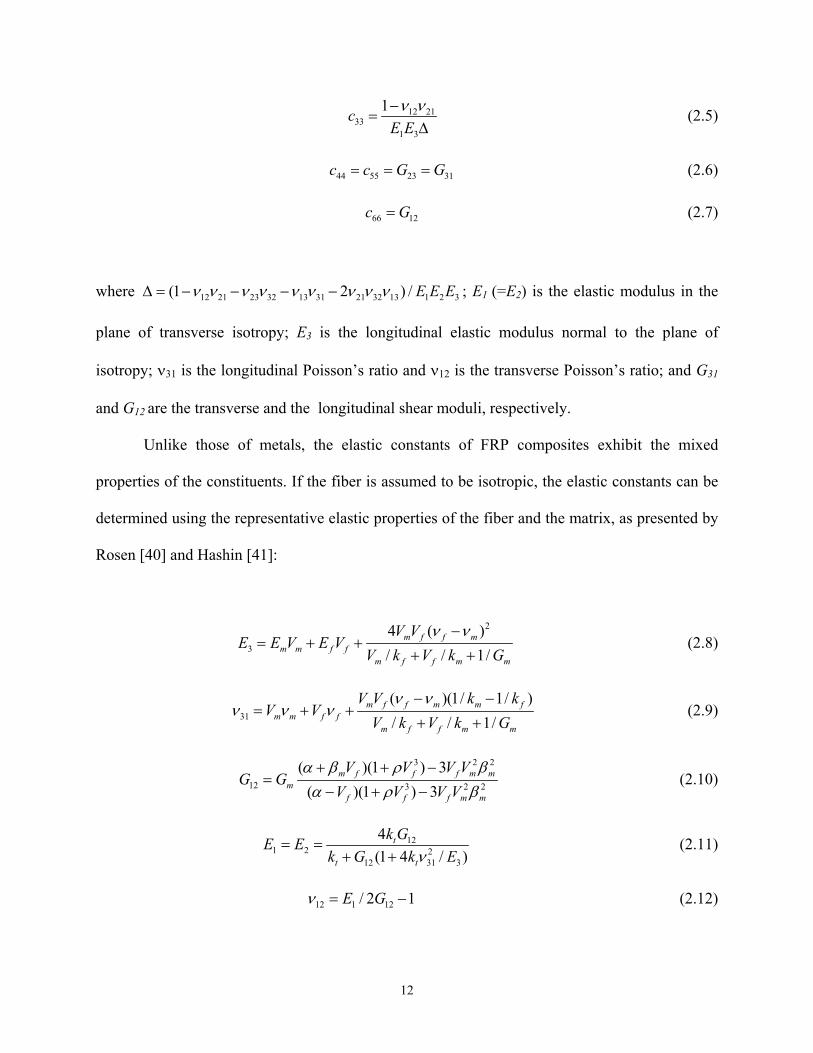

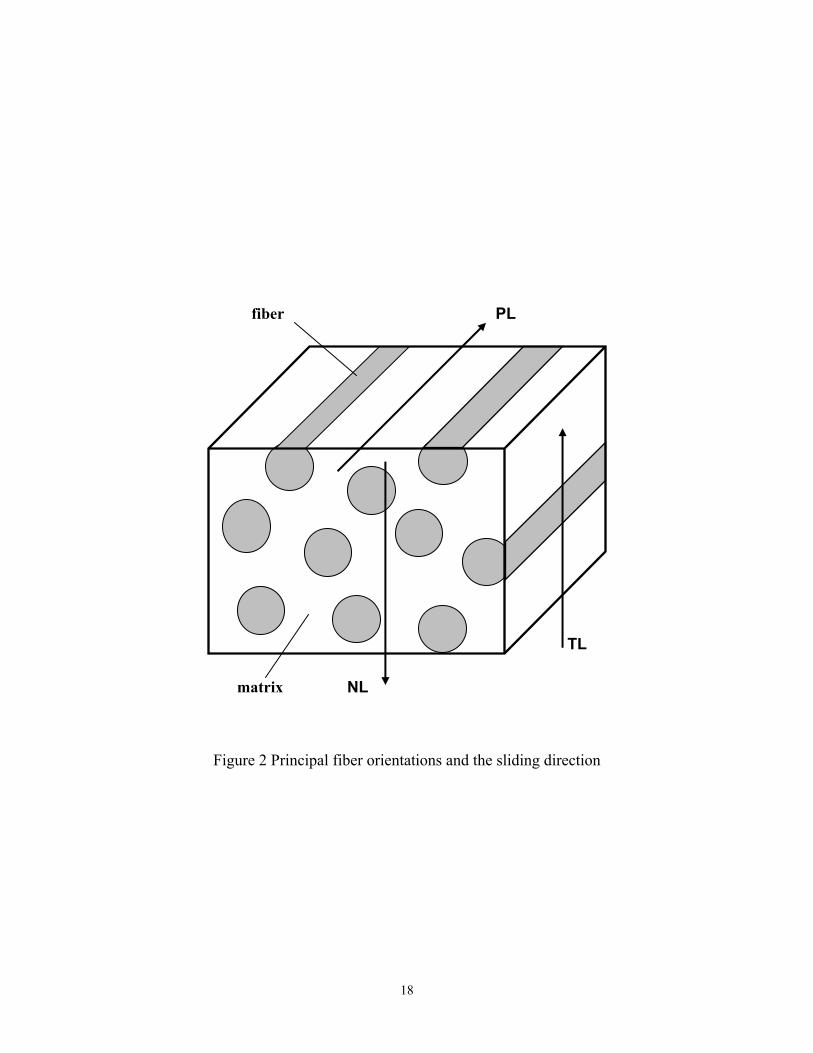
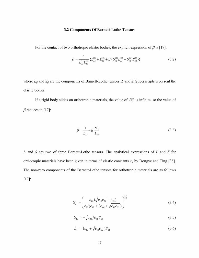
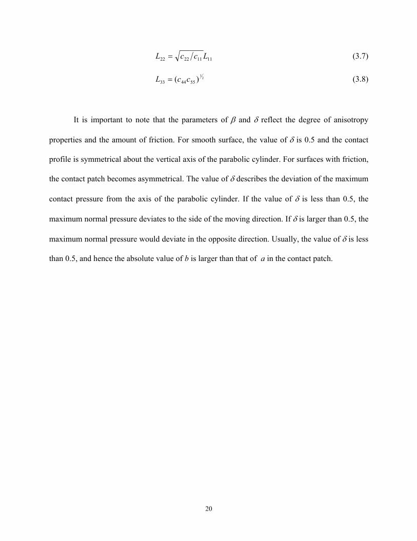
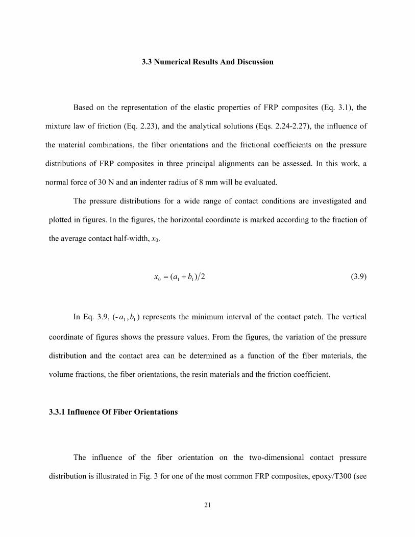


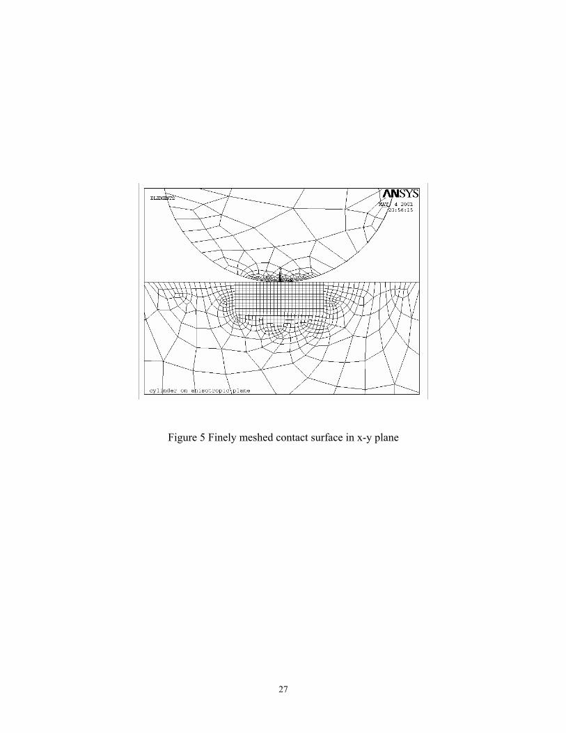

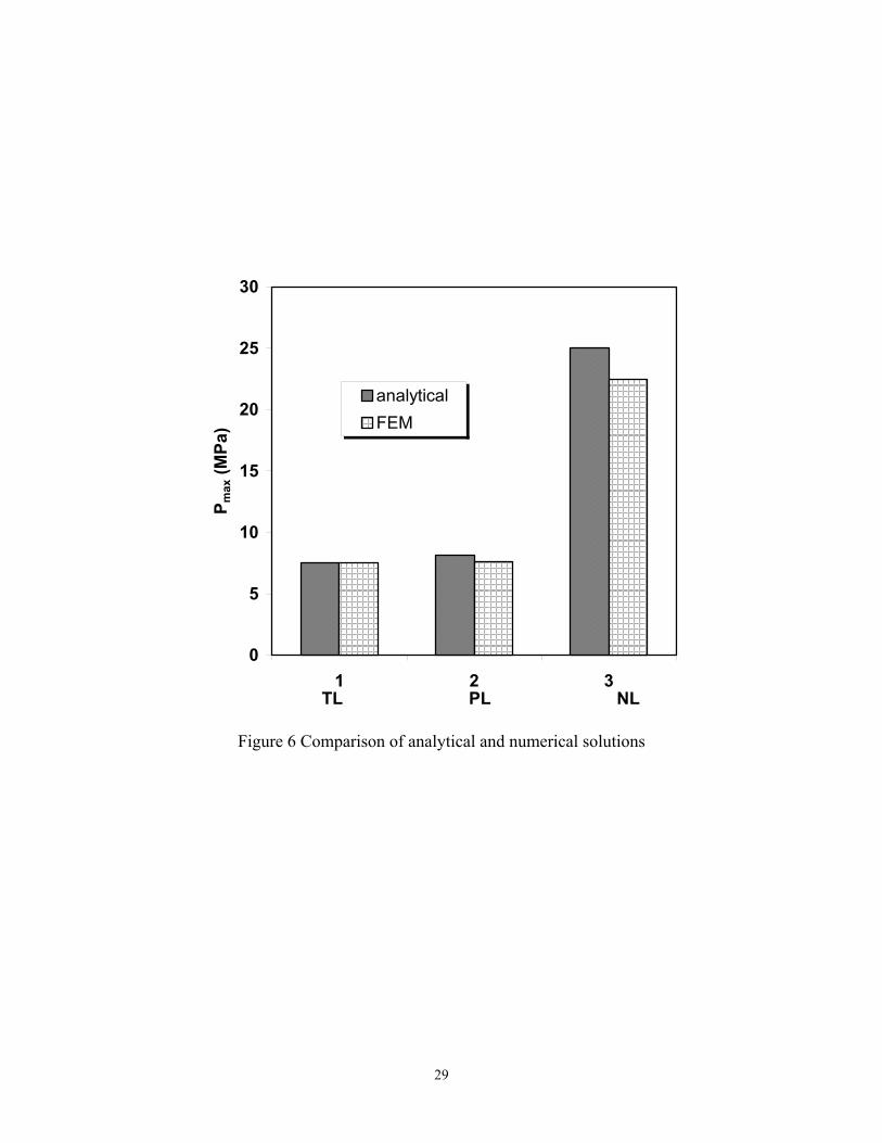


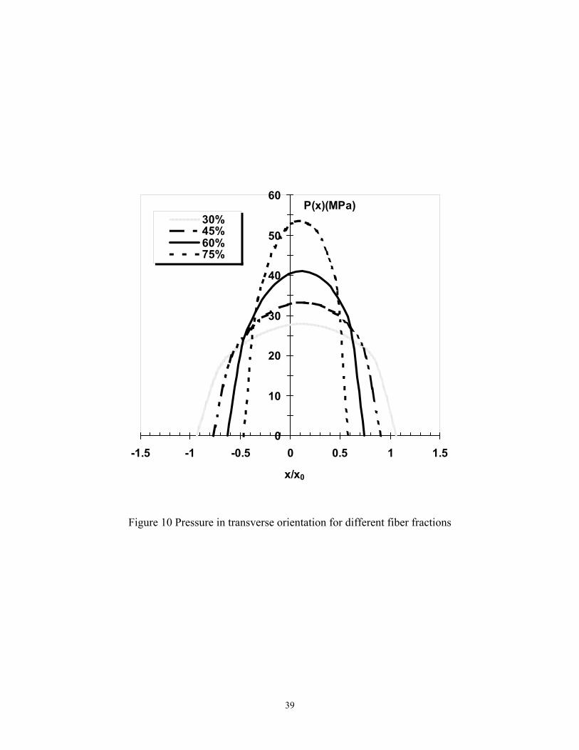
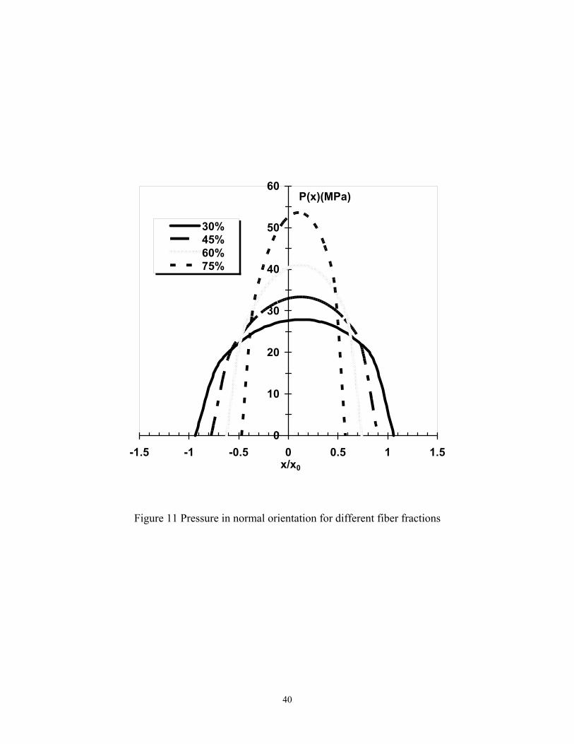
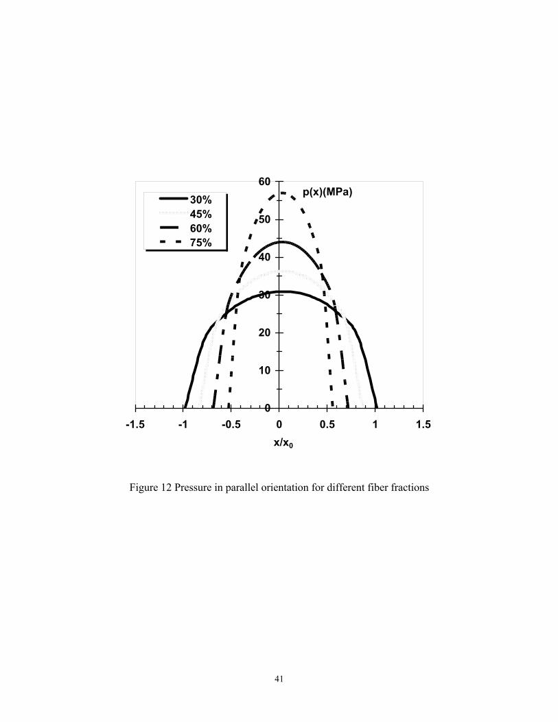

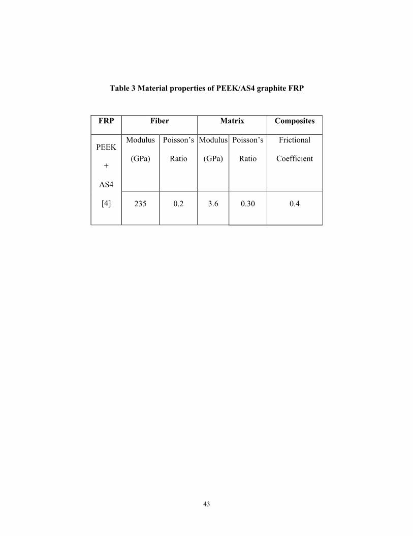
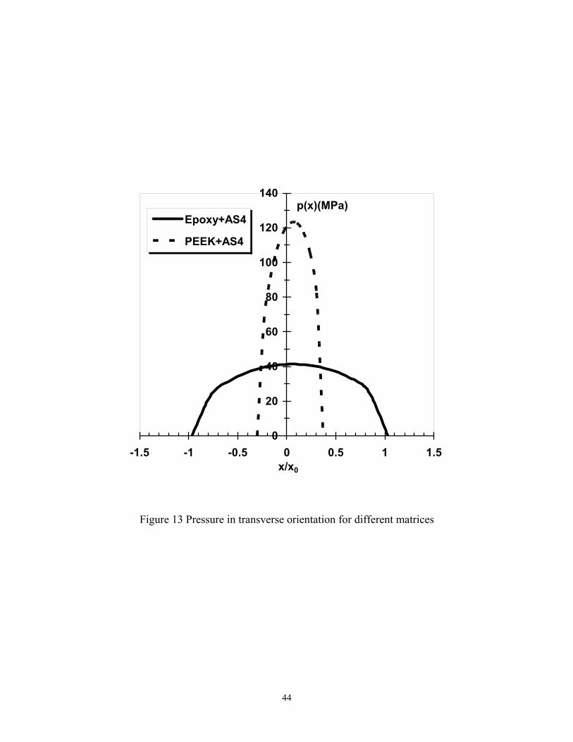


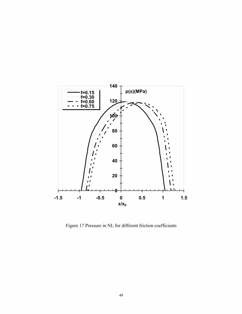


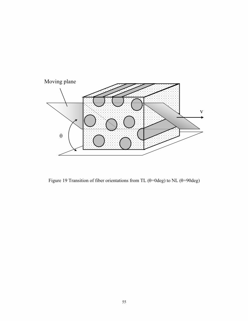

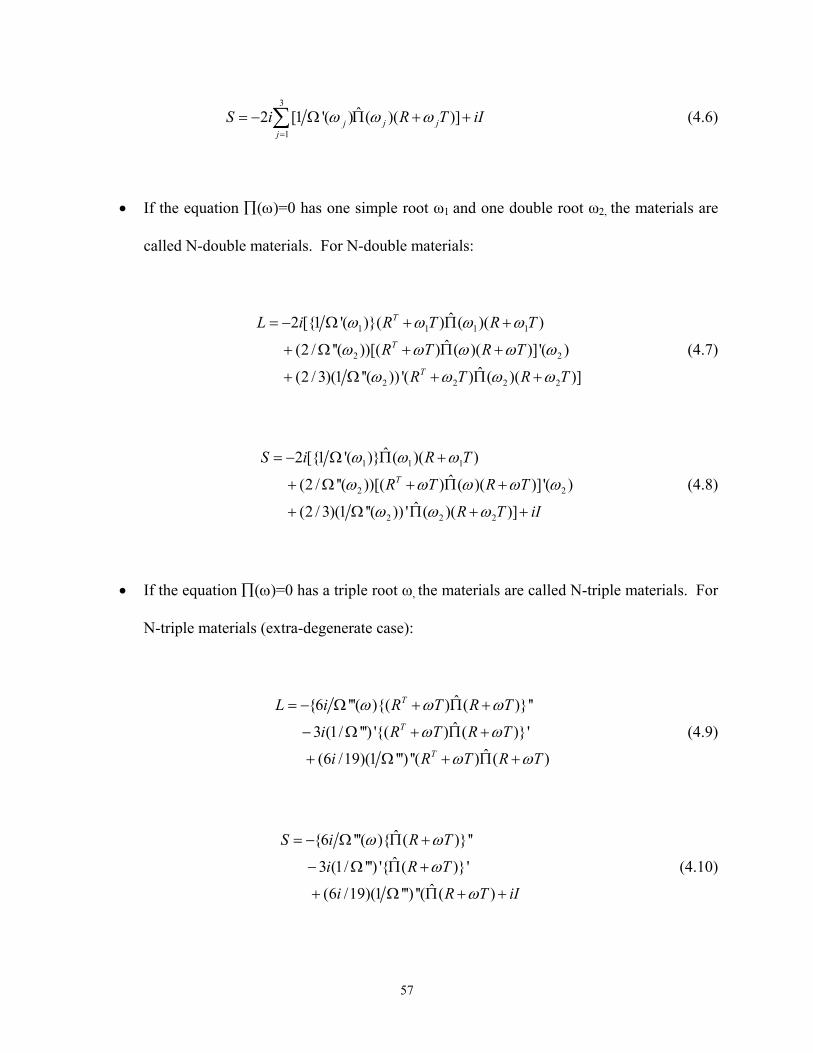


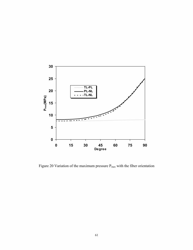


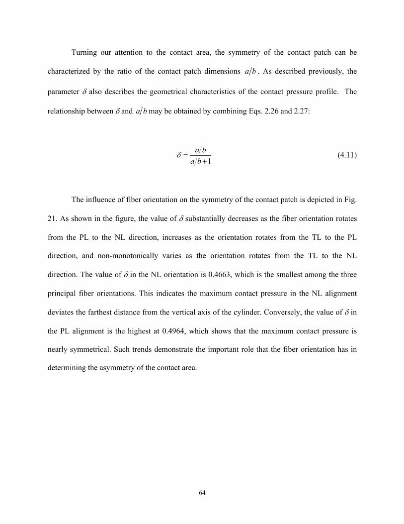


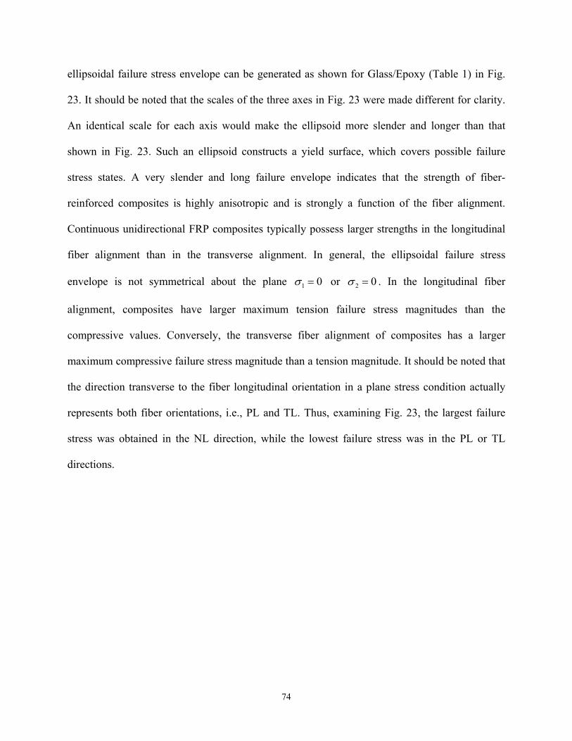
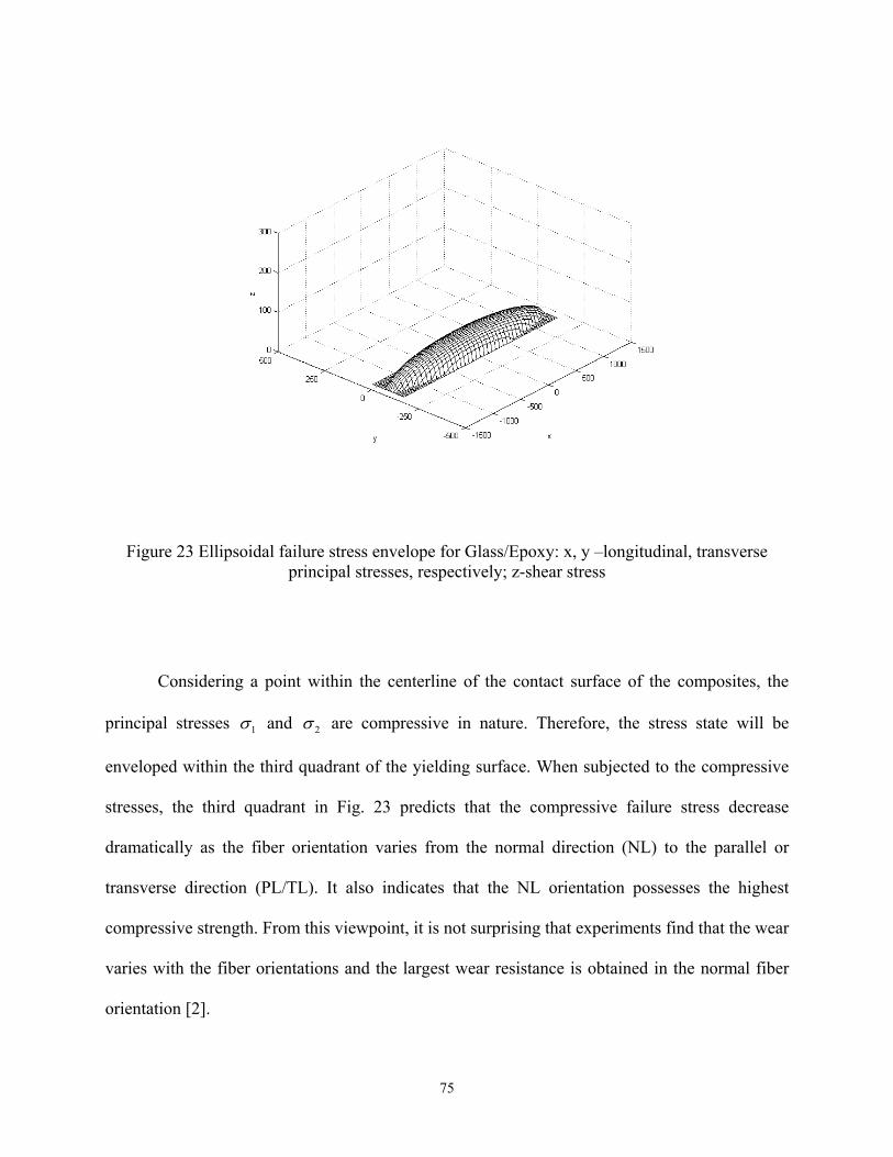


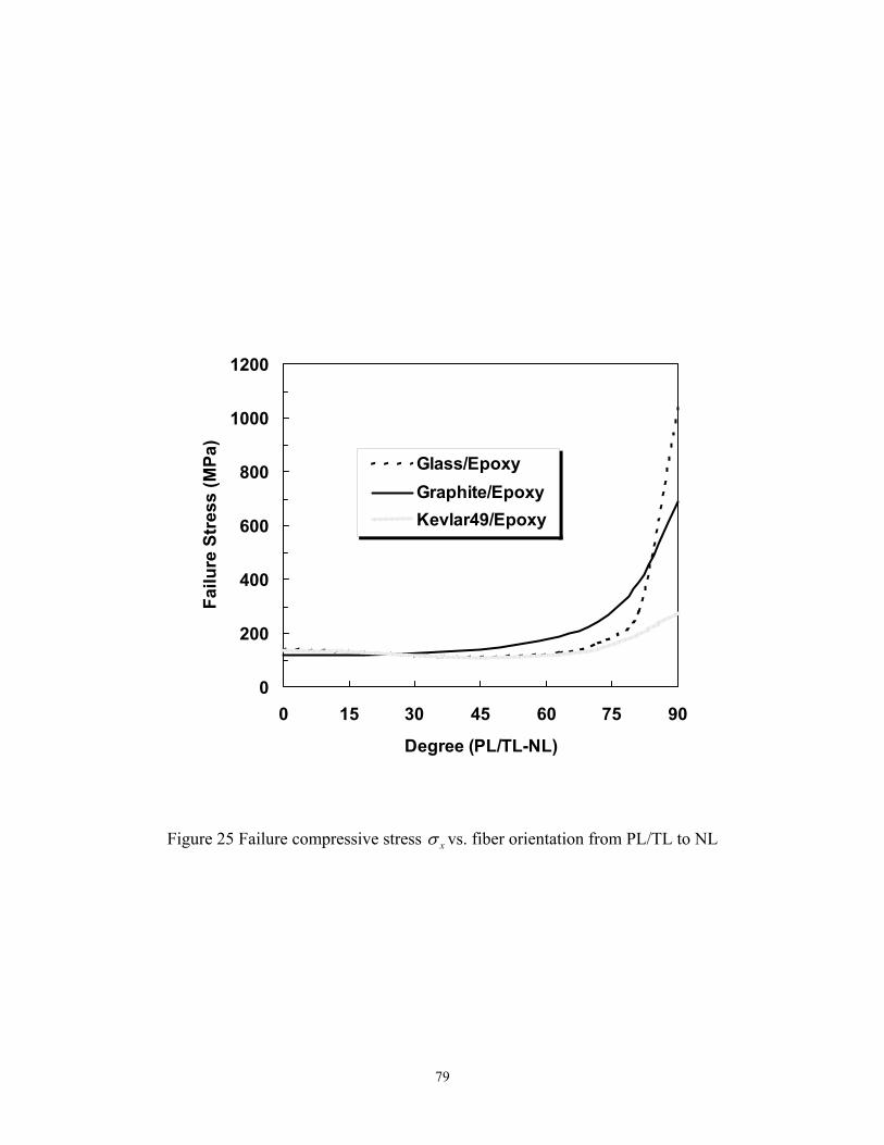


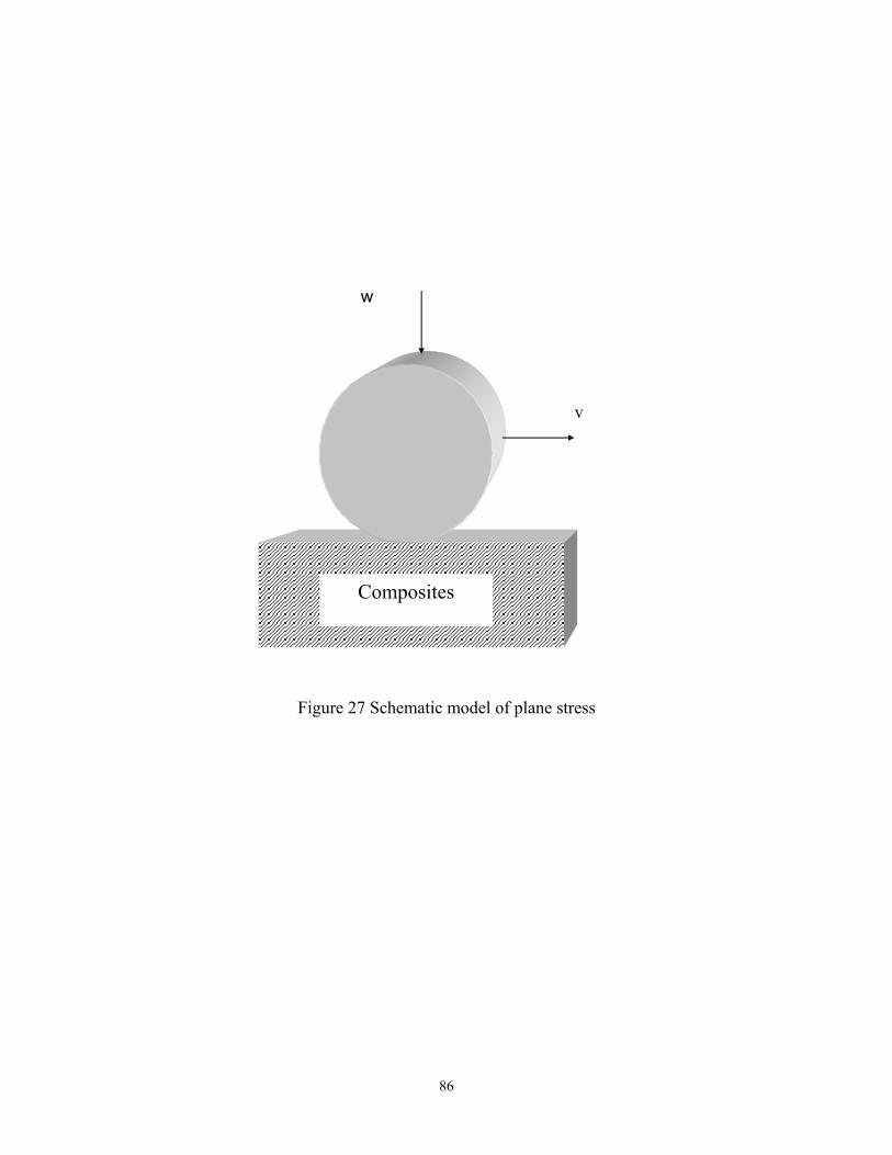


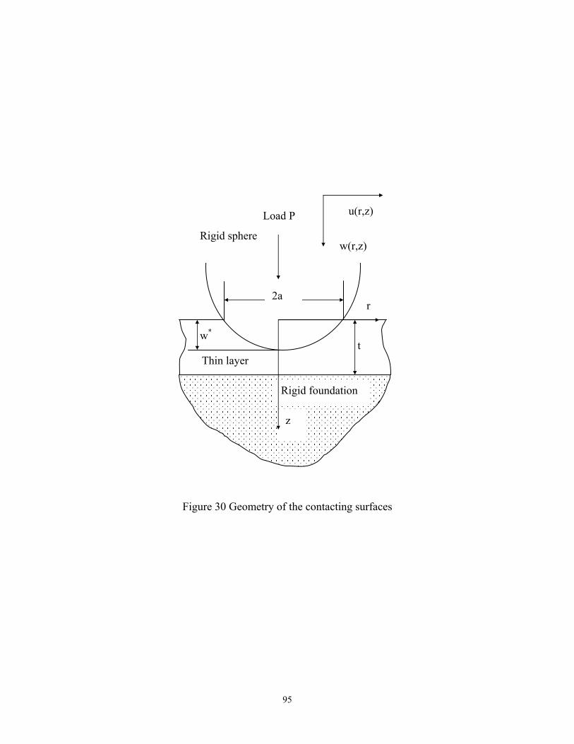


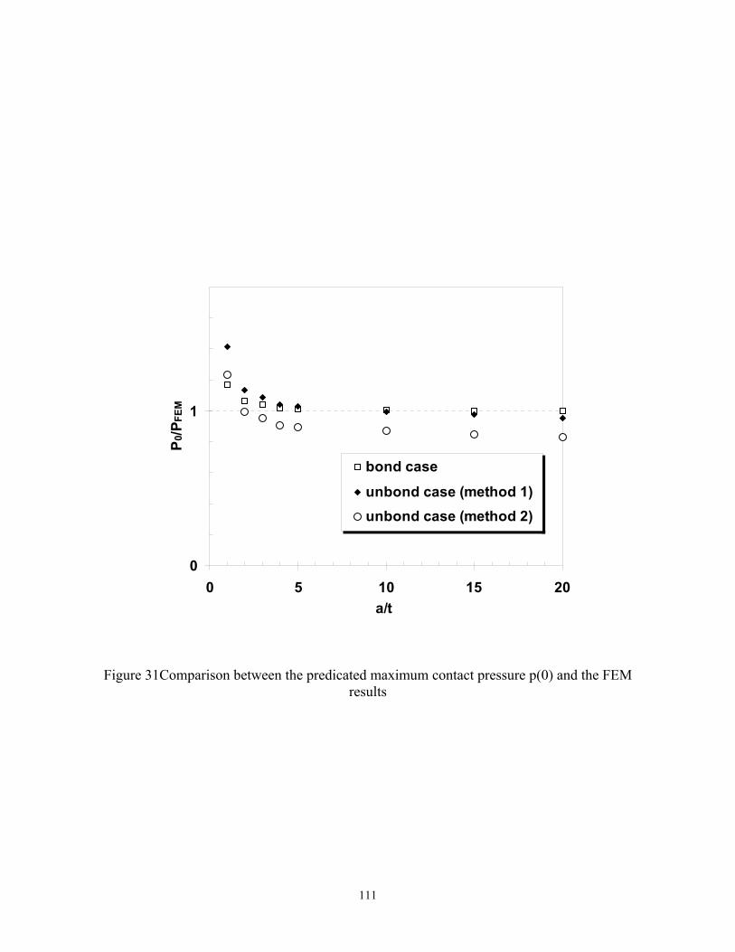
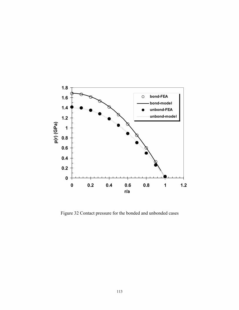


![Studies on Tribological Behavior of Polyamide Filled Jute Fiber-Nano-ZnO Hybrid Composites · 2017. 1. 23. · Erol et al [6] illustrated that the tribological behavior of polymers](https://static.documents.pub/doc/80x56/5fe7fb2eff9bc64ea27f714b/studies-on-tribological-behavior-of-polyamide-filled-jute-fiber-nano-zno-hybrid.jpg)


