Analysis of Wind Tunnel Polar Replicates Using the Modern Design of Experiments (Invited) · ·...

American Institute of Aeronautics and Astronautics

1

Analysis of Wind Tunnel Polar Replicates

Using the Modern Design of Experiments (Invited)

Richard DeLoach*

NASA Langley Research Center, Hampton, Virginia, 23681

John R. Micol†

NASA Langley Research Center, Hampton, Virginia, 23681

The role of variance in a Modern Design of Experiments analysis of wind tunnel data is

reviewed, with distinctions made between explained and unexplained variance. The

partitioning of unexplained variance into systematic and random components is illustrated,

with examples of the elusive systematic component provided for various types of real-world

tests. The importance of detecting and defending against systematic unexplained variance in

wind tunnel testing is discussed, and the random and systematic components of unexplained

variance are examined for a representative wind tunnel data set acquired in a test in which a

missile is used as a test article. The adverse impact of correlated (non-independent)

experimental errors is described, and recommendations are offered for replication strategies

that facilitate the quantification of random and systematic unexplained variance.

Nomenclature

ALPT Model total angle of attack, deg

ANOVA Analysis of variance

AoA, ALP Model angle of attack, deg

ALPTUN Model angle of attack, normal force in vertical plane, deg

BETTUN Model angle of sideslip, normal force in vertical plane, deg

CAF Forebody axial force coefficient (Body and Missile Axis)

CLMNR Non-rolled pitching moment coefficient, tunnel fixed (Missile Axis)

CLL Rolling moment coefficient (Body and Missile Axis)

CLNNR Non-rolled yawing moment coefficient, tunnel fixed (Missile Axis)

CNNR Non-rolled normal force coefficient, tunnel fixed (Missile Axis)

CYNR Non-rolled side force coefficient, tunnel fixed (Missile Axis)

DEL1 Canard #1 deflection angle, deg DEL2 Canard #2 deflection angle, deg

DEL3 Canard #3 deflection angle, deg

DEL4 Canard #4 deflection angle, deg

df Degrees of freedom

F Ration of effects variance to error variance

Fcrit Critical F: Criterion for significant effect

Factor A variable for which levels changes are planned in the course of an experiment

Level A specific value of a factor or independent variable (2° is a level of the factor angle of attack)

LSD Least Significant Difference

Mach Mach number

MDOE Modern Design of Experiments MS Mean Square, also Variance

OFAT One Factor At a Time

* Senior Research Scientist, NASA Langley Research Center, MS 238, 4 Langley Blvd, Hampton, VA 23681,

Associate Fellow. † Ground Facilities Testing Technical Lead for Business Partnership, NASA Langley Research Center, MS 225,

Bldg 1236, Rm 208, Senior Member.

https://ntrs.nasa.gov/search.jsp?R=20100025834 2018-06-14T14:16:04+00:00Z


2

P-value Probability that an effect is due to chance

PHIS Balance roll angle, deg

PS Static pressure, psia

PT Total pressure, psia

Q Dynamic pressure, psia

QA Quality Assurance Response A variable that depends on the values of various factor levels

RN Reynolds number

Sample A collection of N individual data points, where N can be any number, including 1

SS Sum of Squares

TS Tunnel static temperature, deg F

TT Tunnel total temperature, deg F

UPWT Unitary Plan Wind Tunnel

I. Introduction

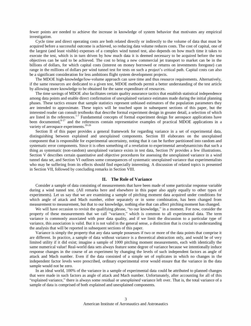
uring the fall of 2000, the aerodynamics of a surface-to-air missile model (Fig. 1) was tested in the Unitary

Plan Wind Tunnel (UPWT) at NASA’s Langley Research Center using a conventional One Factor At a Time

(OFAT) experiment design. The test was designated T1878. The authors were recently asked to examine the data

from T1878 to see how quality and productivity might be improved if the Modern Design of Experiments (MDOE)

were applied in a future study of a similar test article. Of special interest was the question of whether productivity

and quality improvements typically achieved when MDOE methods are applied in conventional fixed-wing and

lifting-body tests could be achieved when the test article is a missile.

This paper reports on the initial phase of this OFAT/MDOE comparison, focusing on an objective assessment the

UPWT measurement environment that is typical of the planning stage of any MDOE experiment design. Since

MDOE data volume requirements depend on the magnitude and nature of the unexplained variance that can be

anticipated in a worst-case scenario, it is useful to obtain as clear an idea of this as is possible as part of the

experiment design. The MDOE method reduces costs by minimizing the volume of data necessary to achieve technical objectives in

a wind tunnel test or in any other type of experiment, a concept that is anathema to conventional wind tunnel testing

strategies that focus on high-volume data collection. The data volume is minimized by changing the levels of

multiple independent variables at the same time for each data point, which imparts substantially more knowledge of

the system’s response characteristics into each point than when independent variables are only changed one factor at

a time, as has been the traditional approach. With more knowledge available to be harvested from each data point,

D

Figure 1. Missile test article used in wind tunnel test.


3

fewer points are needed to achieve the increase in knowledge of system behavior that motivates any empirical

investigation.

Cycle time and direct operating costs are both related directly or indirectly to the volume of data that must be

acquired before a successful outcome is achieved, so reducing data volume reduces costs. The cost of capital, one of

the largest (and least visible) expenses of a complex wind tunnel test, also depends on how much time it takes to

execute the test, which is in turn driven by how much data it is deemed necessary to be acquired before the test objectives can be said to be achieved. The cost to bring a new commercial jet transport to market can be in the

billions of dollars, for which capital costs (interest on money borrowed or returns on investments foregone) can

range in the millions of dollars per wind tunnel test for tests on such a project’s critical path. Capital costs can also

be a significant consideration for less ambitions flight system development projects.

The MDOE high-knowledge/low-volume approach can save time and thus resource requirements. Alternatively,

if the same resources are dedicated to a given test, MDOE methods permit a better understanding of the test article

by allowing more knowledge to be obtained for the same expenditure of resources.

The time savings of MDOE also facilitates certain quality assurance tactics that establish statistical independence

among data points and enable direct confirmation of unexplained variance estimates made during the initial planning

phases. These tactics ensure that sample statistics represent unbiased estimators of the population parameters they

are intended to approximate. These topics will be touched upon in subsequent sections of this paper, but the

interested reader can consult textbooks that describe formal experiment design in greater detail, a selection of which are listed in the references.1-7 Fundamental concepts of formal experiment design for aerospace applications have

been documented,8-17 and the references contain representative examples of practical MDOE applications in a

variety of aerospace experiments.18-26

Section II of this paper provides a general framework for regarding variance in a set of experimental data,

distinguishing between explained and unexplained components. Section III elaborates on the unexplained

component that is responsible for experimental uncertainty, noting that it can be further partitioned into random and

systematic error components. Since it is often something of a revelation to experimental aerodynamicists that such a

thing as systematic (non-random) unexplained variance exists in test data, Section IV provides a few illustrations.

Section V describes certain quantitative and objective procedures for assessing the unexplained variance in a wind

tunnel data set, and Section VI outlines some consequences of systematic unexplained variance that experimentalists

who may be suffering from its effects should find especially interesting. A discussion of related topics is presented in Section VII, followed by concluding remarks in Section VIII.

II. The Role of Variance

Consider a sample of data consisting of measurements that have been made of some particular response variable during a wind tunnel test. (All remarks here and elsewhere in this paper also apply equally to other types of

experiments). Let us say that we are examining a sample of pitching moment data acquired under conditions for

which angle of attack and Mach number, either separately or in some combination, has been changed from

measurement to measurement, but that to our knowledge, nothing else that can affect pitching moment has changed.

We will have occasion to revisit the qualifying phrase, ―to our knowledge,‖ in a moment. For now, consider the

property of these measurements that we call ―variance,‖ which is common to all experimental data. The term

variance is commonly associated with poor data quality, and if we limit the discussion to a particular type of

variance, this association is valid. But it is not valid in the general sense, a distinction that is crucial to understanding

the analysis that will be reported in subsequent sections of this paper.

Variance is simply the property that any data sample possesses if two or more of the data points that comprise it

are different. In practice, a sample of data without variance is a theoretical abstraction only, and would be of very

limited utility if it did exist; imagine a sample of 1000 pitching moment measurements, each with identically the same numerical value! Real-world data sets always feature some degree of variance because we intentionally induce

response changes in the course of an experiment by changing the levels of such independent factors as angle of

attack and Mach number. Even if the data consisted of a simple set of replicates in which no changes in the

independent factor levels were prescribed, ordinary experimental error would ensure that the variance in the data

sample would not be zero.

In an ideal world, 100% of the variance in a sample of experimental data could be attributed to planned changes

that were made in such factors as angle of attack and Mach number. Unfortunately, after accounting for all of this

―explained variance,‖ there is always some residual or unexplained variance left over. That is, the total variance of a

sample of data is comprised of both explained and unexplained components.


4

Explained variance comprises most of the total variance in a typical wind tunnel data set. It is through the

explained variance that we gain new knowledge of the complex relationships between factors such as angle of

attack, Mach number, control surface deflections, etc; and the response variables they influence, such as pressures,

forces, and moments. We are motivated to take the time and bear the expense of wind tunnel testing precisely

because we seek such knowledge. Therefore, lots of variance in aerodynamic response data is a good thing, as long

as the lion’s share of it can be explained in terms of the factor changes that were intentionally made throughout the test. It is the unexplained component of the total variance that constitutes a quality issue, as it is a major contributor

to the uncertainty in test results. Isolating and then carefully quantifying the unexplained variance is therefore an

important (if occasionally overlooked) element of any empirical investigation, including a wind tunnel test.

Of special interest in this report is the fact that the volume of data that must be planned in order to achieve

specified precision goals depends on the level of unexplained variance anticipated in the samples of data to be

acquired in a given measurement environment such as a particular wind tunnel. This means that the minimum

resources that must be budgeted for a successful test, which are a function of the volume of data to be acquired as

argued earlier, also depend on how much unexplained variance is anticipated. Estimating how much unexplained

variance to anticipate is therefore a critical element in formal test planning, playing a role in what is known as

scaling the experiment. It is in the scaling process that the minimum volume of data and the associated resource

requirements to be budgeted are estimated. For a specified precision requirement, data volume requirements are a

sensitive function of the anticipated unexplained variance, so it is important to assess this carefully. There is a corollary to the relationship between specified precision and data volume, which is that unexplained

variance is less a quality issue than a cost issue. With a well-designed test, arbitrarily high levels of precision can be

achieved in any measurement environment as long as a sufficient volume of data is acquired. This is not, as it may

initially seem, an argument in favor of maximizing data volume. Once a volume of data is acquired that is sufficient

to deliver the required level of precision, resources expended on acquiring substantially more data are wasted. A

surprisingly small volume of data is ample to satisfy typical wind tunnel precision requirements. A thorough

understanding of the relationship between precision and unexplained variance can result in significantly more

compact test matrices and smaller testing budgets (time and money) than are typical of conventional wind tunnel

testing strategies that rely on setting an exhaustive combination of factor levels, one factor at a time.

III. The Nature of Unexplained Variance

The unexplained variance in a sample of wind tunnel data has been attributed historically to ―random

experimental error,‖ also known as ―pure error.‖ Pure error is regarded as the result of a number of error processes,

all acting on the data at any instant of time to bias it in a slightly net positive or net negative direction. The algebraic

sum of all such processes is time-dependent so that replicated measurements can be expected to produce slightly different results, no matter how small the interval of time between them. Furthermore, it is assumed that the

resulting errors are random in nature, so that knowledge of the error in any one measurement reveals no information

about the error in any prior, or any subsequent, measurement. (This assumption of independent errors is crucial to

achieving reproducible experimental results from finite samples of data, and unfortunately it is not generally valid

absent explicit effort to assure such independence, about which more presently.)

It is not necessary to understand the specific mechanisms responsible for pure error in order to quantify it.

Random error can simply be regarded as a natural and ubiquitous element of any experimental investigation.

The most common error model that has emerged in conventional wind tunnel testing is that random, chance

variations in the data occur about a sample mean that is stable in time. Under such conditions, while individual

replicates may differ because of ordinary chance variations in the data, sample means are expected to be stationary,

especially for moderately large samples.

One likely reason for the popularity of this model is that its alternative—that sample means change with time—is so inconvenient. Consider a single-point sample of pitching moment data acquired early in the week and then

replicated later in the week. If the sample means were not time invariant, we would have to account for pitching

moment’s dependence on time as well as on such factors as angle of attack and Mach number. This means we would

have to distinguish between the Monday pitching moment, say, and the Friday pitching moment. The entire business

of experimental aeronautics, already a complicated affair, would be all the more complex if our measurements were

not reproducible within ordinary random error, no matter how much time elapses between the measurements. This

possibility is seldom even considered in conventional wind tunnel data acquisition and analysis. The stability of

sample means is simply assumed, and relatively few resources are actually expended to confirm this assumption.

Even fewer resources are routinely expended to defend against the possibility of time-dependent sample means in


5

the event, however unlikely it may seem to be, that Nature would fail to accommodate the researcher with indefinite

intervals of such a convenient level of stability.

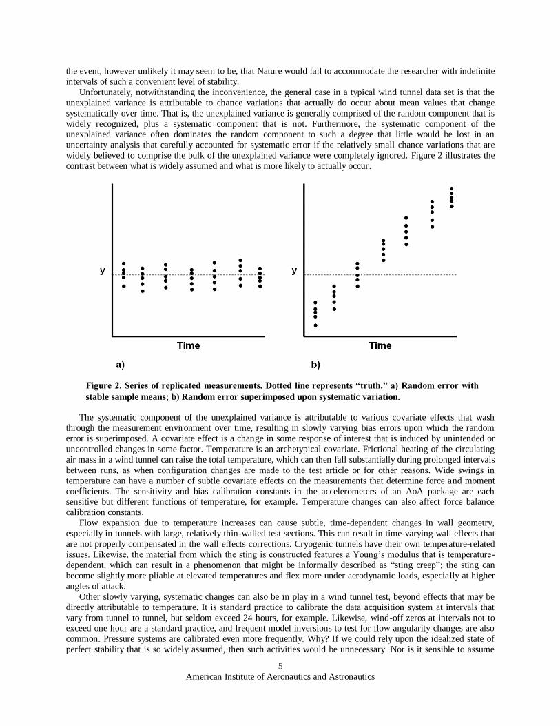
Unfortunately, notwithstanding the inconvenience, the general case in a typical wind tunnel data set is that the

unexplained variance is attributable to chance variations that actually do occur about mean values that change

systematically over time. That is, the unexplained variance is generally comprised of the random component that is

widely recognized, plus a systematic component that is not. Furthermore, the systematic component of the unexplained variance often dominates the random component to such a degree that little would be lost in an

uncertainty analysis that carefully accounted for systematic error if the relatively small chance variations that are

widely believed to comprise the bulk of the unexplained variance were completely ignored. Figure 2 illustrates the

contrast between what is widely assumed and what is more likely to actually occur.

The systematic component of the unexplained variance is attributable to various covariate effects that wash

through the measurement environment over time, resulting in slowly varying bias errors upon which the random

error is superimposed. A covariate effect is a change in some response of interest that is induced by unintended or

uncontrolled changes in some factor. Temperature is an archetypical covariate. Frictional heating of the circulating

air mass in a wind tunnel can raise the total temperature, which can then fall substantially during prolonged intervals

between runs, as when configuration changes are made to the test article or for other reasons. Wide swings in

temperature can have a number of subtle covariate effects on the measurements that determine force and moment

coefficients. The sensitivity and bias calibration constants in the accelerometers of an AoA package are each sensitive but different functions of temperature, for example. Temperature changes can also affect force balance

calibration constants.

Flow expansion due to temperature increases can cause subtle, time-dependent changes in wall geometry,

especially in tunnels with large, relatively thin-walled test sections. This can result in time-varying wall effects that

are not properly compensated in the wall effects corrections. Cryogenic tunnels have their own temperature-related

issues. Likewise, the material from which the sting is constructed features a Young’s modulus that is temperature-

dependent, which can result in a phenomenon that might be informally described as ―sting creep‖; the sting can

become slightly more pliable at elevated temperatures and flex more under aerodynamic loads, especially at higher

angles of attack.

Other slowly varying, systematic changes can also be in play in a wind tunnel test, beyond effects that may be

directly attributable to temperature. It is standard practice to calibrate the data acquisition system at intervals that

vary from tunnel to tunnel, but seldom exceed 24 hours, for example. Likewise, wind-off zeros at intervals not to exceed one hour are a standard practice, and frequent model inversions to test for flow angularity changes are also

common. Pressure systems are calibrated even more frequently. Why? If we could rely upon the idealized state of

perfect stability that is so widely assumed, then such activities would be unnecessary. Nor is it sensible to assume

Figure 2. Series of replicated measurements. Dotted line represents “truth.” a) Random error with

stable sample means; b) Random error superimposed upon systematic variation.


6

that our stability assumptions are secured by such activities; systematic variations can always be in play between

wind-off zeros and model inversions, and between system calibrations. These systematic (non-random) effects may

be small in an absolute sense and difficult to detect without a concerted effort to do so, but in an environment in

which parts per million of unexplained variance can consume the entire error budget of a precision wind-tunnel test,

they can be, and often are, the dominant source of unexplained variance.

IV. Evidence of a Systematic Component of Unexplained Variance

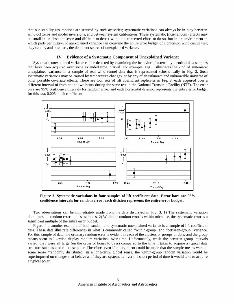
Systematic unexplained variance can be detected by examining the behavior of ostensibly identical data samples

that have been acquired over some extended time interval. For example, Fig. 3 illustrates the kind of systematic

unexplained variance in a sample of real wind tunnel data that is represented schematically in Fig. 2. Such

systematic variations may be caused by temperature changes, or by any of an unknown and unknowable universe of other possible covariate effects. There are four sets of lift coefficient replicates in Fig. 3, each acquired over a

different interval of from one to two hours during the same test in the National Transonic Facility (NTF). The error

bars are 95% confidence intervals for random error, and each horizontal division represents the entire error budget

for this test, 0.005 in lift coefficient.

Two observations can be immediately made from the data displayed in Fig. 3. 1) The systematic variation

dominates the random error in these samples. 2) While the random error is within tolerance, the systematic error is a

significant multiple of the entire error budget.

Figure 4 is another example of both random and systematic unexplained variance is a sample of lift coefficient

data. These data illustrate differences in what is commonly called ―within-group‖ and ―between-group‖ variance. For this sample of data, the ordinary random error is evident in each of the clusters or groups of data, and the group

means seem to likewise display random variations over time. Unfortunately, while the between-group intervals

varied, they were all large (on the order of hours to days) compared to the time it takes to acquire a typical data

structure such as a pitch-pause polar. Therefore, even if an argument could be made that the sample means were in

some sense ―randomly distributed‖ in a long-term, global sense, the within-group random variation would be

superimposed on changes that behave as if they are systematic over the short period of time it would take to acquire

a typical polar.

Figure 3. Systematic variations in four samples of lift coefficient data. Error bars are 95%

confidence intervals for random error; each division represents the entire error budget.


7

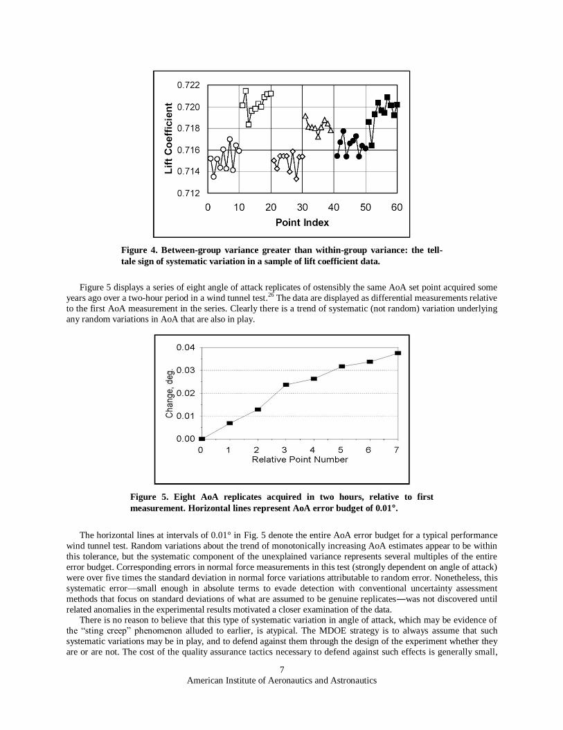
Figure 5 displays a series of eight angle of attack replicates of ostensibly the same AoA set point acquired some

years ago over a two-hour period in a wind tunnel test.26 The data are displayed as differential measurements relative

to the first AoA measurement in the series. Clearly there is a trend of systematic (not random) variation underlying

any random variations in AoA that are also in play.

The horizontal lines at intervals of 0.01° in Fig. 5 denote the entire AoA error budget for a typical performance

wind tunnel test. Random variations about the trend of monotonically increasing AoA estimates appear to be within

this tolerance, but the systematic component of the unexplained variance represents several multiples of the entire

error budget. Corresponding errors in normal force measurements in this test (strongly dependent on angle of attack)

were over five times the standard deviation in normal force variations attributable to random error. Nonetheless, this

systematic error—small enough in absolute terms to evade detection with conventional uncertainty assessment

methods that focus on standard deviations of what are assumed to be genuine replicates―was not discovered until

related anomalies in the experimental results motivated a closer examination of the data. There is no reason to believe that this type of systematic variation in angle of attack, which may be evidence of

the ―sting creep‖ phenomenon alluded to earlier, is atypical. The MDOE strategy is to always assume that such

systematic variations may be in play, and to defend against them through the design of the experiment whether they

are or are not. The cost of the quality assurance tactics necessary to defend against such effects is generally small,

Figure 4. Between-group variance greater than within-group variance: the tell-

tale sign of systematic variation in a sample of lift coefficient data.

Figure 5. Eight AoA replicates acquired in two hours, relative to first

measurement. Horizontal lines represent AoA error budget of 0.01°.


8

and can be regarded as an insurance premium the prudent researcher pays to protect against the larger cost of

inference errors that may occur if such systematic variations go undetected.

The existence of systematic as well as random unexplained variance is not unique to wind tunnel testing. We

provide one interesting non-aero example here for illustration.

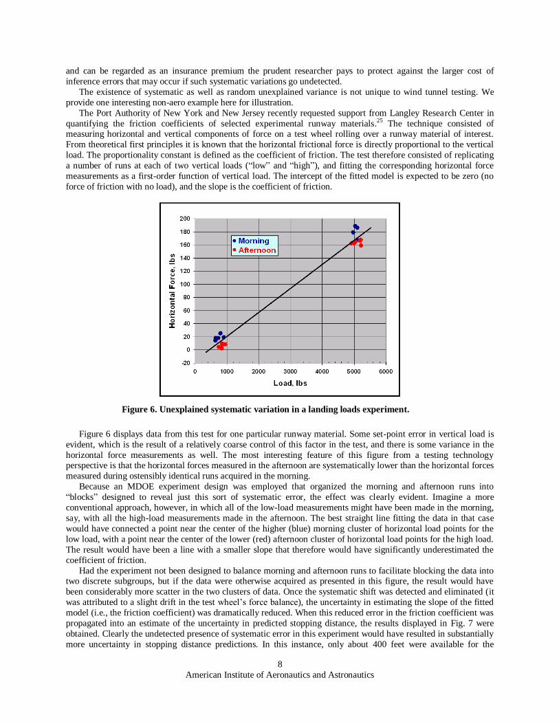
The Port Authority of New York and New Jersey recently requested support from Langley Research Center in

quantifying the friction coefficients of selected experimental runway materials.25 The technique consisted of measuring horizontal and vertical components of force on a test wheel rolling over a runway material of interest.

From theoretical first principles it is known that the horizontal frictional force is directly proportional to the vertical

load. The proportionality constant is defined as the coefficient of friction. The test therefore consisted of replicating

a number of runs at each of two vertical loads (―low‖ and ―high‖), and fitting the corresponding horizontal force

measurements as a first-order function of vertical load. The intercept of the fitted model is expected to be zero (no

force of friction with no load), and the slope is the coefficient of friction.

Figure 6 displays data from this test for one particular runway material. Some set-point error in vertical load is

evident, which is the result of a relatively coarse control of this factor in the test, and there is some variance in the

horizontal force measurements as well. The most interesting feature of this figure from a testing technology perspective is that the horizontal forces measured in the afternoon are systematically lower than the horizontal forces

measured during ostensibly identical runs acquired in the morning.

Because an MDOE experiment design was employed that organized the morning and afternoon runs into

―blocks‖ designed to reveal just this sort of systematic error, the effect was clearly evident. Imagine a more

conventional approach, however, in which all of the low-load measurements might have been made in the morning,

say, with all the high-load measurements made in the afternoon. The best straight line fitting the data in that case

would have connected a point near the center of the higher (blue) morning cluster of horizontal load points for the

low load, with a point near the center of the lower (red) afternoon cluster of horizontal load points for the high load.

The result would have been a line with a smaller slope that therefore would have significantly underestimated the

coefficient of friction.

Had the experiment not been designed to balance morning and afternoon runs to facilitate blocking the data into two discrete subgroups, but if the data were otherwise acquired as presented in this figure, the result would have

been considerably more scatter in the two clusters of data. Once the systematic shift was detected and eliminated (it

was attributed to a slight drift in the test wheel’s force balance), the uncertainty in estimating the slope of the fitted

model (i.e., the friction coefficient) was dramatically reduced. When this reduced error in the friction coefficient was

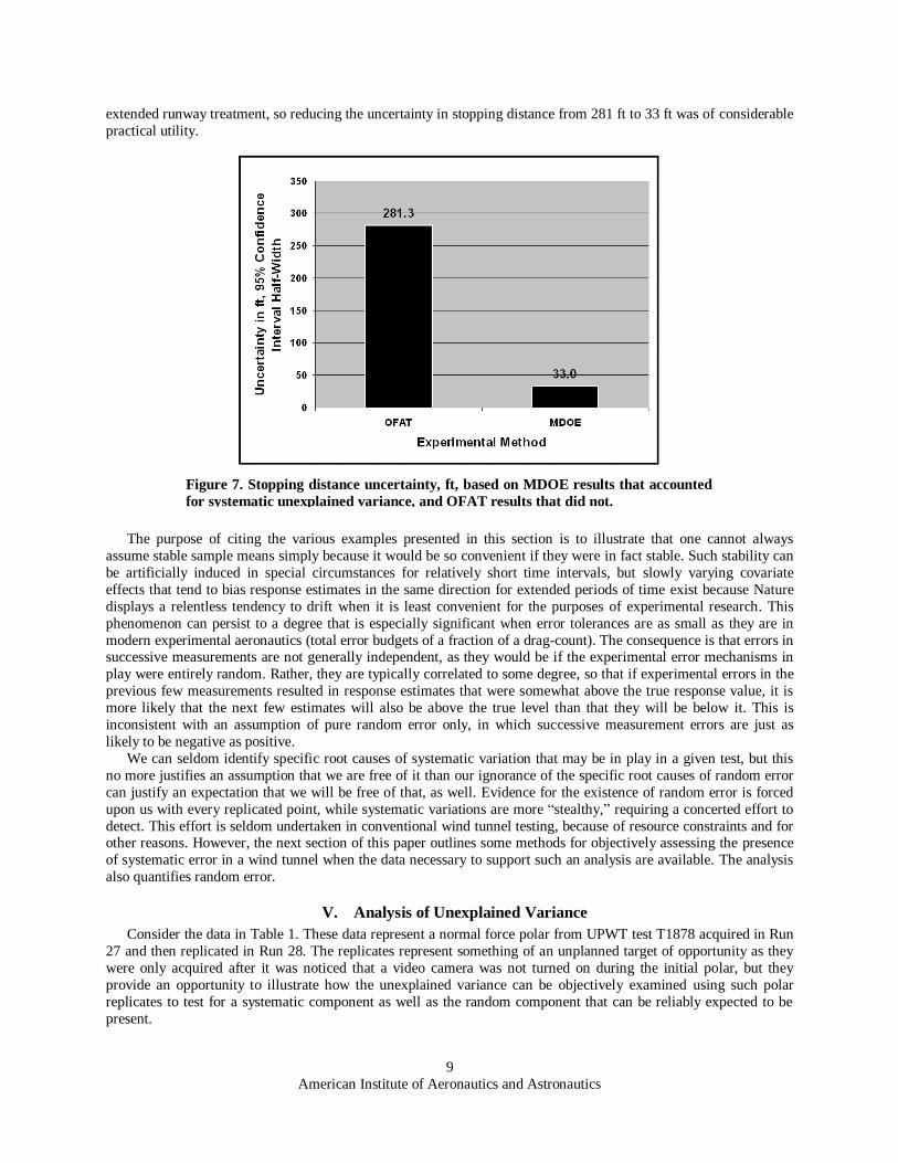
propagated into an estimate of the uncertainty in predicted stopping distance, the results displayed in Fig. 7 were

obtained. Clearly the undetected presence of systematic error in this experiment would have resulted in substantially

more uncertainty in stopping distance predictions. In this instance, only about 400 feet were available for the

Figure 6. Unexplained systematic variation in a landing loads experiment.


9

extended runway treatment, so reducing the uncertainty in stopping distance from 281 ft to 33 ft was of considerable

practical utility.

The purpose of citing the various examples presented in this section is to illustrate that one cannot always

assume stable sample means simply because it would be so convenient if they were in fact stable. Such stability can

be artificially induced in special circumstances for relatively short time intervals, but slowly varying covariate

effects that tend to bias response estimates in the same direction for extended periods of time exist because Nature

displays a relentless tendency to drift when it is least convenient for the purposes of experimental research. This

phenomenon can persist to a degree that is especially significant when error tolerances are as small as they are in

modern experimental aeronautics (total error budgets of a fraction of a drag-count). The consequence is that errors in successive measurements are not generally independent, as they would be if the experimental error mechanisms in

play were entirely random. Rather, they are typically correlated to some degree, so that if experimental errors in the

previous few measurements resulted in response estimates that were somewhat above the true response value, it is

more likely that the next few estimates will also be above the true level than that they will be below it. This is

inconsistent with an assumption of pure random error only, in which successive measurement errors are just as

likely to be negative as positive.

We can seldom identify specific root causes of systematic variation that may be in play in a given test, but this

no more justifies an assumption that we are free of it than our ignorance of the specific root causes of random error

can justify an expectation that we will be free of that, as well. Evidence for the existence of random error is forced

upon us with every replicated point, while systematic variations are more ―stealthy,‖ requiring a concerted effort to

detect. This effort is seldom undertaken in conventional wind tunnel testing, because of resource constraints and for other reasons. However, the next section of this paper outlines some methods for objectively assessing the presence

of systematic error in a wind tunnel when the data necessary to support such an analysis are available. The analysis

also quantifies random error.

V. Analysis of Unexplained Variance

Consider the data in Table 1. These data represent a normal force polar from UPWT test T1878 acquired in Run

27 and then replicated in Run 28. The replicates represent something of an unplanned target of opportunity as they

were only acquired after it was noticed that a video camera was not turned on during the initial polar, but they

provide an opportunity to illustrate how the unexplained variance can be objectively examined using such polar

replicates to test for a systematic component as well as the random component that can be reliably expected to be

present.

Figure 7. Stopping distance uncertainty, ft, based on MDOE results that accounted

for systematic unexplained variance, and OFAT results that did not.


10

The data displayed in Table 1 were preprocessed by fitting each of the two normal force polars with cubic

splines, from which force estimates were made at the design-point angles of attack rather than the angles of attack

for which the data were actually acquired. This ensured that at a given angle of attack, normal force differences

could be attributed to variance in the response measurements and not to ALPTUN set-point errors.

The mean and standard deviation in the mean of the 12 differential normal force values were computed, as was a t-statistic expressing the mean as a multiple of the standard deviation in the mean. Absent any systematic difference

between the two polars, the true differential normal force value at any give angle of attack is expected to be zero.

Ordinary chance variations in the data due to random experimental error preclude any one differential normal force

value from being precisely zero except by chance, but the mean of all such measurements should be very nearly

zero.

Table 1: Replicated Normal Force Polars from UPWT T1878.

Mach 1.6, PHIS=0, All Canard Deflections = 0.

Figure 8. Mean difference between CNNR levels in Runs 27 and 28 for 12 angles of

attack. Any differences within shaded area are statistically indistinguishable from zero.


11

The critical two-tailed t-statistic for 11 degrees of freedom and a significance level of 0.05 can be determined

readily from tabulated values or from standard statistical software. Its value is 2.201, which means that any

measured t-value with an absolute value less than this corresponds to a random variable (in this case, the mean

difference in CNNR levels from Run 27 to Run 28) that cannot be distinguished from zero with at least 95%

confidence. Taking this as the criterion, the data in Table 1 do not support a rejection of the null hypothesis that no

systematic difference exists between the CNNR polars acquired in Run 27 and Run 28, and we therefore infer that no significant covariate effects are in play that affect CNNR, or if they are, the elapsed time between these two

polars (less than six minutes) may have been insufficient for a significant shift to have occurred. Figure 8 displays

the test of this null hypothesis graphically, with the shaded area encompassing the range of t-values corresponding to

random variables that cannot be distinguished from zero with at least 95% confidence, based on a sample of 12

measurements and the standard error estimated for the CNNR data. The CNNR t-statistic is clearly within this range.

We tested for a systematic difference between runs 27 and 28 for the other five forces and moments in the same

way, with results that are displayed in Fig. 9.

Figure 9 reveals no significant difference between runs 27 and 28 for the three moments (rolling, pitching, and

yawing) as well as for normal force, but it indicates that we can reject the null hypothesis of no systematic difference

for axial force and side force with no more than a 5% probability of an inference error.

It should be noted that we are only able to make inferences with a given level of confidence about the response

variables for which systematic variation was detected (axial and side force). For the other four responses, we cannot make an inference of ―no systematic error.‖ For those responses we can only say that if any systematic error is in

play, it is too small to detect with 95% confidence given the levels of random error and the volume of data available

for analysis.

The pair-wise comparisons made between runs 27 and 28 for multiple forces and moments have a particular

disadvantage because the probability of an inference error is less when only one pair of polars is compared than

when more than one are compared. There are 15 unique pairs for six polars, for example, and if the probability of an

inference error is 0.05 (one in 20) for each of 15 inferences, then the probability that all 15 inferences are correct is

0.9515 = 0.46, meaning that the overall probability of at least one inference error is 0.54. That is, it is likely (p > 0.5)

that there will be some inference error. Accounting for six force/moment comparisons for each of 15 polar pairs

increases the overall error probability for pair-wise comparisons from 54% (likely) to 99% (highly likely). A two-

way analysis of variance (ANOVA) avoids such high inference error probabilities for multiple comparisons. Test T1878 featured a number of polar replicates designated Quality Assurance Polars. Six ostensibly identical

Quality Assurance Polars were commonly acquired in wind tunnel tests at Langley Research Center in this

timeframe (around 2000), with three acquired in succession near the beginning of the test and a similar set of three

acquired near the end. The intent was to use each group of three replicated polars to quantify short-term variance,

Figure 9. Mean difference between force and moment levels in Runs 27 and 28

for 12 angles of attack. Any differences within the shaded area are statistically

indistinguishable from zero.


12

and to use any significant observed differences between the group means as an indication of longer-period

systematic variation, or a departure from a state of ―statistical control‖ in which sample means are time-invariant.

As with the unplanned replicates in Runs 27 and 28, the quality assurance polars were first fitted using cubic

splines in order to estimate forces and moments at common factor levels (integer angle of attack values), minimizing

the effect of set-point error. Table 2 displays the six resulting CNNR quality assurance polars.

An analysis of variance was performed on the data in Table 2. Computational details are beyond the scope of this

paper but the reader can consult standard texts on this subject.27 Reference 16 provides a tutorial description of

ANOVA applications in wind tunnel data analysis.

The basic idea behind an analysis of variance is to partition the variance in a sample of data into constituent

components. For the data in Table 2, the variance associated with changes that are experienced from one row to the

next is quantified, as is the variance associated with changes that occur from column to column. The total variance

of the entire data set is also quantified, as is any component of variance that cannot be attributed to changes across

columns, or changes across rows. This latter, residual variance is assumed to be attributable to ordinary chance

variations in the data. Row-wise variation is associated with changes in CNNR that are induced by changing angle

of attack, and represent in that sense a component of the total variance that we can describe as ―explained‖ by the

ALPTUN changes. We are not as interested in row-wise variation for this analysis as we are in column-wise variation, since our intent is to test for systematic variation over time. We wish to determine whether the column-

wise variance is large compared to the residual or random error variance. Absent any systematic changes from

column to column (that is, over time), the column-wise variance and residual error variance should be nominally the

same.

Table 3 summarizes the ANOVA calculations for the data in Table 2. There is one row in the ANOVA table

dedicated to each of the sources of variation. The first three columns to the right of the source names contain

computed values for sums of squares, degrees of freedom, and their ratio—variance or Mean Square. The next

column is a list of F-statistics representing the ratio of each variance component to the error mean square. The row-

wise variance is seen to be 293,031 times larger than the random error variance, emphasizing the rather

unremarkable fact that changing angle of attack over a range in this instance of 13 degrees does indeed result in

much greater changes in CNNR than are attributable to random error. The F-statistic for column-wise variation, however, is much smaller, at 1.49.

Table 2. Six CNNR Quality Assurance Polars from UPWT T1878. Mach 2.16, PHIS=0, All Canard

Deflections = 0.

Table 3. ANOVA Table for CNNR Data of Table 2.


13

The fact that column-wise variance is greater than random error variance (F > 1) suggests that perhaps there is in

fact some systematic variation from column to column; however, the data samples are comprised of a finite number

of measurements that are each influenced by random fluctuations in the data, so it is possible for departures from a

ratio of 1 to be attributable to the waxing and waning of numerator and denominator due to ordinary experimental

error. We therefore examine the P-value.

The P-value column contains numbers representing the probability that F-statistics as large as those observed could be attributable entirely to chance variations in the data. For the row-wise variation, this probability is

vanishingly small. Given the level of random error, essentially no combination of random fluctuations in the

numerator and denominator of the F-statistic would be expected to cause such an enormous ratio. Since it is so

unlikely that random variations in the data are responsible for the large F-statistic, we infer that some non-random

(i.e., systematic) effect explains it, and we attribute the large F to the systematic row-wise variation in angle of

attack displayed in Table 2.

The P-value for the column-wise variation is 0.207. Unlike the P-value for row-wise variation, this is not a

particularly small number. There is better than one chance in five that the ratio of column-wise variance to error

variance could be as high as 1.49 just due to random fluctuations of a magnitude observed in each of these values,

even if there is no systematic variation from column to column in Table 2. Therefore the data do not provide

sufficient evidence to reject a Null Hypothesis that no systematic column-wise variation is in play. We therefore

conclude in the case of the CNNR data, that if there are such systematic variations, they are too small to detect with at least 95% confidence.

If we adopt as a criterion that any hypothesized effect, such as systematic variation across columns (or rows),

must be detectable with at least 95% confidence before we will report it as a non-random phenomenon, this

establishes 0.05 as a critical P-value. For any phenomenon with a P-value in excess of 0.05, there is more than a 5%

probability that it will occur by chance, and therefore less than a 95% probability that it can be attributed to non-

chance events. In the case of Table 3, there is a negligible probability that the row-wise variation is due to chance

and so a near certainty that the variance is due to systematic changes (in this case, ALPTUN variations), while the

opposite circumstances apply to the column-wise variations; a relatively high probability of chance variations

implies a relatively low probability of some systematic causal effect.

The Fcrit column in ANOVA Table 3 is an F-statistic that corresponds to a critical P-value of 0.05, and also

depends on the number of degrees of freedom that are available to estimate the variance in the numerator and denominator of the F-statistic. Column-wise variance would have to exceed error variance by a factor of the Fcrit

value in order for the probability that it is a due to chance variations to drop below 0.05 in Table 3. This is then the

condition that must be met to justify reporting a systematic cause for a given component of variance (row-wise or

column-wise) with at least 95% confidence. In the case of row-wise variation, the fact that the measured F-value of

293,061 exceeded the Fcrit value of 1.92 by such a large margin provides the overwhelming evidence supporting a

conclusion that CNNR varies with ALPTUN (not unanticipated, as noted before, but a reassuringly consistent

result). The fact that the measured F-value for column-wise variance is only 1.49 while the Fcrit value is 2.37

implies that there is insufficient variation across columns to attribute it to anything other than random error.

The square root of the Mean Square error from the ANOVA table (1.82E-05 in Table 3) is just the standard

random error (―one sigma‖). For the normal force data, the value is 0.0043. The ANOVA calculations thus quantify

the random component of the unexplained variance, as well as testing for any systematic component.

ANOVA calculations were performed for the coefficients of axial force, pitching moment, rolling moment, yawing moment, and side force, in addition to normal force (CNNR). The resulting P-values, F-values, and Fcrit

values are summarized in Table 4.

Table 4. Summary of ANOVA results for systematic variation in T1878 QA polar means.


14

The ANOVA results of Table 4 are generally consistent with the paired t-test results that are displayed in Fig. 9.

In both cases, systematic variation between replicated polars of axial force and side force can be unambiguously

detected. The ANOVA results in Table 4 also reveal a significant shift between replicated yawing moment polars

that Fig. 9 does not indicate with 95% or more confidence for Runs 27 and 28. Nonetheless, the largest statistically

insignificant t-statistic for Runs 27 and 28 was for yawing moment, and it is possible that the absence of an effect

large enough to detect with 95% confidence is attributable to the short time interval (less than six minutes) between runs 27 and 28. There is no evidence of significant systematic between-polar variation for normal force, rolling

moment, or pitching moment, either in the analysis of runs 27 and 28, or in the analysis of the designated QA polars.

This analysis of variance indicates systematic (non-random) differences between two or more polar means.

When a polynomial model is used to fit response data to factors that have undergone a common centering and

scaling transformation, the mean of the fitted data corresponds to the y-intercept of the model. This is independent

of the order of the polynomial or the number of independent variables, so in the case of a simple function of one

variable such as an angle of attack polar, the polar mean has the same interpretation. A systematic difference in the

means of two ostensibly identical polars therefore represents a shift in the intercept or ―DC component‖ of the fitted

function. This intercept can serve as a tracer for the effects of covariates washing through the system.

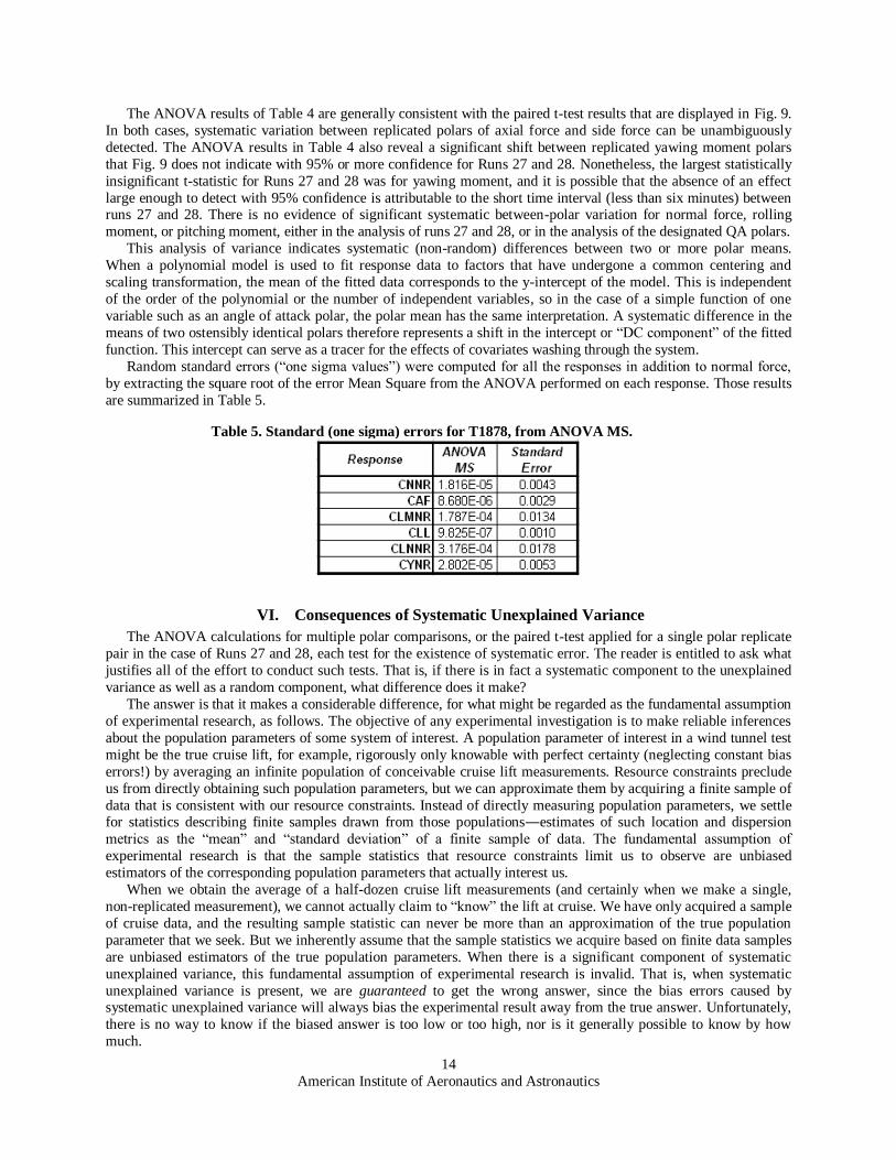
Random standard errors (―one sigma values‖) were computed for all the responses in addition to normal force,

by extracting the square root of the error Mean Square from the ANOVA performed on each response. Those results

are summarized in Table 5.

VI. Consequences of Systematic Unexplained Variance

The ANOVA calculations for multiple polar comparisons, or the paired t-test applied for a single polar replicate

pair in the case of Runs 27 and 28, each test for the existence of systematic error. The reader is entitled to ask what

justifies all of the effort to conduct such tests. That is, if there is in fact a systematic component to the unexplained

variance as well as a random component, what difference does it make?

The answer is that it makes a considerable difference, for what might be regarded as the fundamental assumption

of experimental research, as follows. The objective of any experimental investigation is to make reliable inferences

about the population parameters of some system of interest. A population parameter of interest in a wind tunnel test

might be the true cruise lift, for example, rigorously only knowable with perfect certainty (neglecting constant bias

errors!) by averaging an infinite population of conceivable cruise lift measurements. Resource constraints preclude

us from directly obtaining such population parameters, but we can approximate them by acquiring a finite sample of

data that is consistent with our resource constraints. Instead of directly measuring population parameters, we settle for statistics describing finite samples drawn from those populations―estimates of such location and dispersion

metrics as the ―mean‖ and ―standard deviation‖ of a finite sample of data. The fundamental assumption of

experimental research is that the sample statistics that resource constraints limit us to observe are unbiased

estimators of the corresponding population parameters that actually interest us.

When we obtain the average of a half-dozen cruise lift measurements (and certainly when we make a single,

non-replicated measurement), we cannot actually claim to ―know‖ the lift at cruise. We have only acquired a sample

of cruise data, and the resulting sample statistic can never be more than an approximation of the true population

parameter that we seek. But we inherently assume that the sample statistics we acquire based on finite data samples

are unbiased estimators of the true population parameters. When there is a significant component of systematic

unexplained variance, this fundamental assumption of experimental research is invalid. That is, when systematic

unexplained variance is present, we are guaranteed to get the wrong answer, since the bias errors caused by systematic unexplained variance will always bias the experimental result away from the true answer. Unfortunately,

there is no way to know if the biased answer is too low or too high, nor is it generally possible to know by how

much.

Table 5. Standard (one sigma) errors for T1878, from ANOVA MS.


15

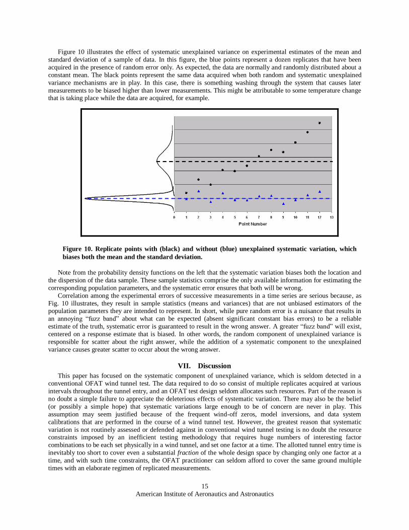
Figure 10 illustrates the effect of systematic unexplained variance on experimental estimates of the mean and

standard deviation of a sample of data. In this figure, the blue points represent a dozen replicates that have been

acquired in the presence of random error only. As expected, the data are normally and randomly distributed about a

constant mean. The black points represent the same data acquired when both random and systematic unexplained

variance mechanisms are in play. In this case, there is something washing through the system that causes later

measurements to be biased higher than lower measurements. This might be attributable to some temperature change that is taking place while the data are acquired, for example.

Note from the probability density functions on the left that the systematic variation biases both the location and

the dispersion of the data sample. These sample statistics comprise the only available information for estimating the

corresponding population parameters, and the systematic error ensures that both will be wrong.

Correlation among the experimental errors of successive measurements in a time series are serious because, as

Fig. 10 illustrates, they result in sample statistics (means and variances) that are not unbiased estimators of the population parameters they are intended to represent. In short, while pure random error is a nuisance that results in

an annoying ―fuzz band‖ about what can be expected (absent significant constant bias errors) to be a reliable

estimate of the truth, systematic error is guaranteed to result in the wrong answer. A greater ―fuzz band‖ will exist,

centered on a response estimate that is biased. In other words, the random component of unexplained variance is

responsible for scatter about the right answer, while the addition of a systematic component to the unexplained

variance causes greater scatter to occur about the wrong answer.

VII. Discussion

This paper has focused on the systematic component of unexplained variance, which is seldom detected in a

conventional OFAT wind tunnel test. The data required to do so consist of multiple replicates acquired at various

intervals throughout the tunnel entry, and an OFAT test design seldom allocates such resources. Part of the reason is

no doubt a simple failure to appreciate the deleterious effects of systematic variation. There may also be the belief

(or possibly a simple hope) that systematic variations large enough to be of concern are never in play. This

assumption may seem justified because of the frequent wind-off zeros, model inversions, and data system

calibrations that are performed in the course of a wind tunnel test. However, the greatest reason that systematic

variation is not routinely assessed or defended against in conventional wind tunnel testing is no doubt the resource constraints imposed by an inefficient testing methodology that requires huge numbers of interesting factor

combinations to be each set physically in a wind tunnel, and set one factor at a time. The allotted tunnel entry time is

inevitably too short to cover even a substantial fraction of the whole design space by changing only one factor at a

time, and with such time constraints, the OFAT practitioner can seldom afford to cover the same ground multiple

times with an elaborate regimen of replicated measurements.

Figure 10. Replicate points with (black) and without (blue) unexplained systematic variation, which

biases both the mean and the standard deviation.


16

In the missile aerodynamics test considered in this paper, for example, the following factors and factor levels

were of interest: four canards with five deflections each, 31 levels of roll angle, 19 angle of attack levels, and two

Mach numbers, or 5x5x5x5x31x19x2=736,250 possible factor combinations. Resources were exhausted after

examining a subset of 5,575 of these factor combinations one factor at a time. This amounts to 0.76% of the total,

not an atypical percentage in a conventional OFAT test.

There is an implicit assumption common in OFAT wind tunnel testing that those factor combinations that must be left unexamined due to resource constraints, typically 99+ % of the total, are somehow irrelevant for practical

purposes, or at least that they are of a much lower priority than the factor combinations there is time to examine.

This does not even account for the responses at intermediate factor levels that also go unexamined when discrete

factor levels are physically set one factor at a time. There actually are some configurations that may not be of

interest―certain non-aerodynamic control surface combinations, for example―but it strains credulity to suggest

that we can leave 99+ % of the information on the table in a typical wind tunnel test and still achieve most of the

desirable objectives.

Faced with the impossible task of individually examining, with limited resources, what is for practical purposes

an infinite number of factor combinations, it is no wonder that the typical wind tunnel researcher is hesitant to spend

time going over ground already covered by replicating earlier measurements. It generally seems more prudent, under

these circumstances, to allocate limited wind tunnel time to exploring parts of the design space that have not yet

been examined, rather than repeating measurements that have already been acquired. One reason for diminished concerns over systematic variations in an OFAT wind tunnel test was cited earlier:

Standard operating procedures in a conventional wind tunnel test include certain tactics specifically designed to

eliminate systematic shifts in the response estimates. These include frequent (typically hourly) wind-off zeros,

model inversions designed to detect changes in flow angularity and other systematic changes, and regularly

scheduled calibrations of such subsystems as pressure transducers and the data acquisition system. All of these

activities convey a certain sense of security that any systematic variation otherwise in play will have been

eliminated.

Unfortunately, while this strategy probably represents the most effective approach to controlling the

measurement environment that is practical given typical resource constraints, there is plenty of evidence to suggest

that it is not enough. For example, the various citings in this paper of significant systematic variation were all taken

from wind tunnel tests in which such tactics were routinely applied. Clearly, periodic corrections for the cumulative effects of systematic variation will have no effect on variations

occurring in the interim; the correction applied as a result of a wind-off zero only addresses systematic shifts at that

one instant in time. Such a correction does nothing to stop covariate effects that are in play, and data acquired

between wind-off zeros will continue to be influenced by any such effects during that interval.

The analysis above revealed systematic variation when there was an unscheduled replication of Run 27 in test

T1878, for example, even though the replicated polar, Run 28, was executed within six minutes of Run 27. Wind-off

zeros, model inversions, and data system calibrations simply cannot be executed often enough to compensate for

conditions that change this rapidly. Likewise, systematic response shifts were observed in the six Quality Assurance

Polars that were subjected to a formal ANOVA. While some variation might not have been unanticipated between

polars acquired at the start and at the end of the test, systematic variations were in fact observed among polars that

were acquired back-to-back, as in the case of runs 27 and 28. The individual lift coefficient replicates in Fig. 3 from

another test displayed systematic (non-random) changes of several multiples of the entire error budget over time intervals that are not dissimilar from the intervals between wind off zeros. Systematic, unplanned changes in angle

of attack are seen in Fig. 5 for yet another test to have changed at an average rate of about 0.02° per hour, enough to

exceed the entire error budget by a factor of two in an interval no greater than is typically permitted between wind-

off zeros.

These observations might be characterized as anecdotal, involving only a small percentage of all of the polars

acquired in the tests that have been cited. On the other hand, they represent a large percentage of the specific polars

drawn from these tests to be examined for evidence of unexplained systematic variation. It is not unlikely that other

data in these tests were also influenced by the kinds of systematic unexplained variance that adversely impacts

statistical independence, and leads to the kinds of bias errors represented schematically in Fig. 10.

Conventional techniques designed to ensure stability in the measurement environment by frequent calibrations

and adjustments represent one approach to coping with systematic variation, but there is another. Instead of attempting to perfect the measurement environment by using brute strength, as it were, to force Nature to conform to

our desire for a convenient but unnatural level of stability, we can simply allow Nature to have her own way as she

will in any case. We can then compensate for the systematic changes that will inevitably occur, by how we execute

our experiments and how we analyze the data they produce. That is, instead of trying to squeeze out the systematic


17

variation, we can compensate for it by designing our experiments in such a way as to ensure that experimental errors

are independent whether systematic variation is in play or not. This, in turn, will ensure that the means and standard

deviations of finite data samples with which we are forced to contend by resource constraints will in fact represent

unbiased estimators of their corresponding population parameters. This is key to any successful experiment.

In actual practice, some combination of tactics is desirable. We should make all efforts that are cost effective to

contain the range of systematic variation, while adopting other quality assurance tactics to account for the systematic variation that it is not practical to eliminate entirely. A detailed exposition of such tactics is beyond the scope of this

paper, but they are centered on randomizing the set-point order of test matrices to the maximum practical extent,

blocking or grouping subsets of data in such a way as to facilitate the detection and elimination of systematic shifts

that may occur between them, and replicating data over relatively short and relatively long intervals, to permit the

assessment of ordinary random error and the detection and quantification of longer-term unexplained variance.

These tactics, which have been employed for decades outside the aerospace industry, are described in detail in

essentially every textbook on experiment design. A few standard texts are listed in the references,1-7 as are papers

focused more on this specific topic.10-12

Perhaps the most important reason to provide sufficient test resources to cope with unexplained systematic

variation is that factor effects can be reproduced from test to test with relatively high precision, but covariate effects

cannot. They tend to be localized phenomena, differing from test to test. Unless sufficient precautions are taken, the

results of a replicated wind tunnel test are virtually guaranteed to differ from the test it is attempting to reproduce, to a degree dictated by the uncontrolled differences in covariate effects between the two tests. To the extent that this

difference is large compared to established tolerance requirements, as it often is in the case of high-precision wind

tunnel testing (especially performance testing), reproducibility of results in experimental aeronautics will continue to

be a problem. These difficulties are only exacerbated by a testing philosophy that is predicated on the assumption

that covariate effects are either negligible, or small enough that they can be physically eliminated by within-test

corrective actions (wind-off zeros, etc.) that are only applied as often as it is convenient to do.

Unexplained systematic variance generally remains in play at troublesome levels even after all conventional

options to induce stability in the measurement environment have been exhausted. In commonly occurring

circumstances, the resulting systematic errors dominate the random errors that receive so much more attention.

There is another reason that systematic unexplained variance is undesirable, besides the extent to which resulting

systematic errors might be inconsistent with specific tolerance levels. Computations of the standard deviation are always valid as long as no blunders are made in the calculation, as the standard deviation simply represents a

prescribed formula for one particular dispersion metric. However, common interpretations applied to the standard

deviation depend on the distributional properties of the data. Specifically, such rules of thumb as ―two standard

deviations encompass 95% of the residuals‖ are only valid if the residuals are normally distributed, which they are

not if the unexplained variance features a significant systematic component. For this reason, the replicated polars

from runs 27 and 28 of T1878 would be of limited utility in assessing the uncertainty in axial force and side force

results obtained in that test. At the very least, the systematic component of unexplained variance would have to be

taken into account in order to use these data to properly assess the uncertainty.

When covariate effects inflate variance estimates as in Fig. 10, it is of greater concern than the fact that

statements about the uncertainty in response estimates might be improperly represented. When experimental data are

fitted to independent variables to develop a certain class of high-precision mathematical response models describing

system response, a judgment must be made about each candidate term in the math model. Each term will be retained or rejected, based on the size of its coefficient relative to the uncertainty in estimating that coefficient. The

magnitude of the coefficient must be large compared to the standard error in estimating it in order to justify retaining

that term in the model. If variance estimates are inflated, it could cause an artificially low estimate of signal to noise

for a model term that is relatively small, but nonetheless significant. This could cause the term to be erroneously

rejected from the model, an example of a ―Type II inference error.‖ The resulting model might then fail to reveal an

interaction between two factors, for example, or misrepresent some other aspect of the response surface. This could

cause a loss of insight into the underlying physical process, as well as an error in predicting response levels for some

prescribed combination of factors.

A few remarks are in order about the distinction that should be made between statistical significance and

physical significance. A statistically significant effect is simply one that can be distinguished unambiguously from

the noise of ordinary random error. Usually, when an effect is described by an analyst as ―significant,‖ this is the sense in which the word is meant.

However, not all statistically significant effects are large enough to matter; it is possible for an effect to be

significant statistically, but not physically. This is especially true in the case of experimental data acquired with very

high-precision measurement systems, in relatively quiescent measurement environments. In such cases it may be


18

possible to detect an effect that is large compared to a very low background noise level, but is nonetheless so small

as to be of no practical interest.

Consider again the analysis performed on the polar replicates from runs 27 and 28 in test T1878. A statistically

significant difference was detected between the polar means for axial force coefficient and for side force coefficient.

That is, the difference in polar means was large enough that it was unlikely to be due to ordinary random error. For

axial force, the difference in polar means was 0.0020, or 20 counts. The corresponding shift in side force was 0.0111, or 111 counts. Are these shifts large enough to be of concern? For the researcher seeking fractional drag

count precision, a 20-count axial force shift in six minutes would no doubt be troublesome, but if greater tolerance

were acceptable in this particular test, then a 20-count shift might not be important. Similar remarks apply to side

force. There might still be some concern about what kinds of shifts could occur over intervals significantly longer

than six minutes, of course.

A statistically significant F-value in the ANOVA that was applied to Quality Assurance Polars from runs 24-26

and runs 211-213 implied a detectible difference in two or more polar means for some of the responses. However,

there was no information as to which polars were similar and which were different, or how different they were.

A number of tests can be applied to determine how different each polar is from the rest of the polars when an

ANOVA indicates significant differences. Details of the ANOVA method are beyond the scope of this paper, but Fig. 11, which displays axial force polar means for all six QA runs that were examined, illustrates the basic concept.

Here, the difference between each polar mean and the grand mean of all six polars is plotted as a function of the

date/time each polar was acquired (defined as the mid-point between start and end of acquisition). The temporal

clustering of the six polars into two groups of three is evident. The horizontal lines are spaced at the Least

Significant Difference (LSD) corresponding to a 95% confidence level. By definition of the LSD, any two points

displaced from each other by more than the distance between two adjacent horizontal lines in this figure are different

by an amount that can be detected with 95% confidence, while points that do not differ by more than this amount

cannot be distinguished with at least 95% confidence. Error bars represent 95% confidence intervals for the random

component of unexplained variance.

Figure 11 illustrates that the differences in axial force polar means are not necessarily large in absolute terms,

compared for example to the magnitude of random error. This means that while some of the differences are large

enough to detect unambiguously in the presence of random error in play at the time, they are not necessarily large enough to matter. For example, the axial force LSD of 0.0034 (34 counts) is exceeded by four polar pairs, for which

the largest difference, between runs 25 and 212, is 49 counts. Shifts from one polar to the next were larger than

random experimental error, a traditionally criterion for concern, but no precision requirements were documented for

the T1878 test. It therefore remains an article of subjective interpretation as to whether the observed shifts in axial

force were large enough to be of concern. The same can be said for side force, for which statistically significant

Figure 11. Quality Assurance polar means (polynomial intercepts) for axial force in T1878, relative to

average axial force QA polar mean. Horizontal lines represent Least Significant Differences.


19

differences were observed in both the paired t-test involving runs 27 and 28, and the ANOVA for the six QA polars.

This highlights the utility of achieving a documented consensus during the planning stages of a test as to what size

of each observed effect (change in measured responses) is important from a practical perspective. At the very least,

this can provide an objective basis for assessing the uncertainty in experimental results.

We close this discussion with an observation that the Quality Assurance Polars available from T1878 are of a

meager and rather unsatisfactory kind, in that limited replicates were only acquired at the very beginning and very end of the test. This provides what is in effect a single degree of freedom estimate of the long-period systematic

unexplained variance in this test. The original purpose of clustering polar replicates in groups featuring three back-

to-back polars was to assess short-term unexplained variance, but such a grouping is not necessary for this purpose

and short-term systematic variation of the kind that was observed confounds these estimates in any case. A more

effective approach to assessing random, pure error is to make variance calculations from data for which some effort

has been made to ensure that the experimental errors are independent.

It is also better to space polar replicates at longer intervals to test for covariate effects. This provides more

degrees of freedom for the estimate of unexplained systematic variance and also helps illuminate any trends in the

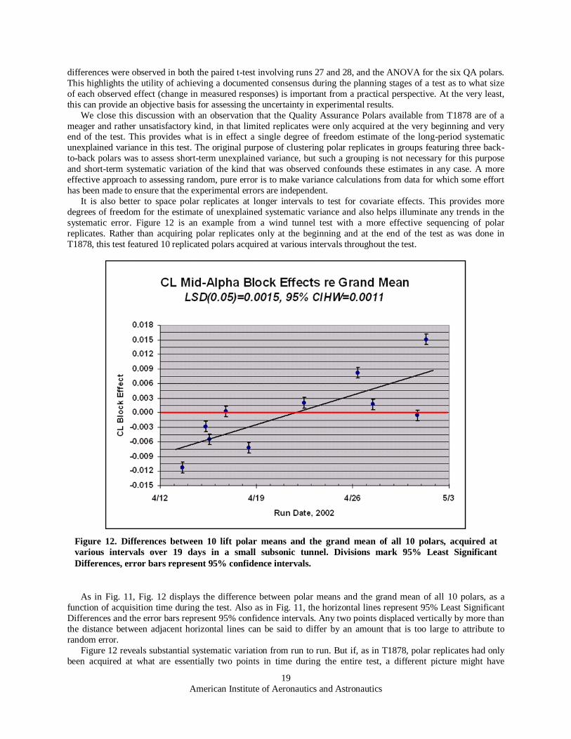
systematic error. Figure 12 is an example from a wind tunnel test with a more effective sequencing of polar

replicates. Rather than acquiring polar replicates only at the beginning and at the end of the test as was done in

T1878, this test featured 10 replicated polars acquired at various intervals throughout the test.

As in Fig. 11, Fig. 12 displays the difference between polar means and the grand mean of all 10 polars, as a

function of acquisition time during the test. Also as in Fig. 11, the horizontal lines represent 95% Least Significant

Differences and the error bars represent 95% confidence intervals. Any two points displaced vertically by more than

the distance between adjacent horizontal lines can be said to differ by an amount that is too large to attribute to

random error.

Figure 12 reveals substantial systematic variation from run to run. But if, as in T1878, polar replicates had only

been acquired at what are essentially two points in time during the entire test, a different picture might have

Figure 12. Differences between 10 lift polar means and the grand mean of all 10 polars, acquired at

various intervals over 19 days in a small subsonic tunnel. Divisions mark 95% Least Significant

Differences, error bars represent 95% confidence intervals.


20

emerged. For example, imagine that polar replicates had only been acquired on April 17 (the fourth polar mean in

Fig. 12) and again two weeks later, on May 1 (second polar from the right). The polar means would not have

differed by as much as the 95% Least Significant Difference, and we would have inferred that there was no evidence

for systematic variation in this test. Similarly, it is difficult to assess the true long-term systematic variance in play

during T1878 from only two samples.

VIII. Concluding Remarks

The intent of this paper has been to examine the data from a representative missile wind tunnel test to assess

improvements that might be made in similar tests in the future by using techniques common to the Modern Design

of Experiments (MDOE). A certain amount of tutorial material was presented to introduce the MDOE focus on

variance and its analysis, which features a partitioning into explained and unexplained components. Unexplained variance was further partitioned into random and systematic components.

The systematic component of unexplained variance was described as a major impediment to reproducibility in

wind tunnel testing. Because of the systematic variance detected in the axial force and side force data of T-1878,

these two responses are expected to be the most difficult to reproduce. They are, unfortunately, key factors in

determining missile range and accuracy. Likewise, the yawing moment, a key accuracy control factor, also displays

systematic variance that is likely to have an adverse impact on reproducibility. No evidence was found for

systematic variation in normal force, rolling moment, or pitching moment.

It appears likely that if a future test of this type were to embrace quality assurance tactics used in MDOE testing

to insure independent (not systematic) experimental errors, the results would be more reproducible. Certain

productivity advantages not directly covered in this paper are also likely to be realized. These are related to the

MDOE practice of instilling more information into each data point by changing multiple factors at a time, which results in the need for significantly fewer points and an attendant savings in direct operating costs and cycle time. It

is virtually certain that an MDOE design would also enable the exploration of significantly more of the design space

than there was time to examine with conventional OFAT testing methods in T1878.

Acknowledgments

This work was supported by the NASA Aeronautics Test Program Office. Figure 4 was produced from data

acquired and analyzed by Dr. Michael Hemsch. The authors acknowledge the special assistance of Mr. Floyd

Wilcox in selecting the coordinate system used for the missile data analysis in this paper and for other helpful

suggestions.

References 1Box, G. E. P., Hunter, W. G., and Hunter, J. S., Statistics for Experimenters, 2nd Ed., John Wiley and Sons, New York, 2005. 2Box, G. E. P., and Draper, N. R., Response Surfaces, Mixtures, and Ridge Analyses, 2nd Ed., John Wiley and Sons, New

York, 2007. 3Montgomery, D. C., Peck, E. A., and Vining, C. G., Introduction to Linear Regression Analysis, 4th Ed., John Wiley and

Sons, New York, 2006. 4Diamond, W. J., Practical Experiment Designs for Engineers and Scientists, Van Nostrand Reinhold, New York, 1981. 5Myers, R. H., and Montgomery, D. C., Response Surface Methodology: Process and Product Optimization Using Designed

Experiments, John Wiley and Sons, New York, 1995. 6Cochran, W. G., and Cox, G. M., Experimental Designs, 2nd Ed., Wiley Classics Library Edition, Wiley, New York, 1992. 7Montgomery, D. C., Design and Analysis of Experiments, 7th Ed., John Wiley and Sons, New York, 2009. 8DeLoach, R., ―Applications of Modern Experiment Design to Wind Tunnel Testing at NASA Langley Research Center,‖

AIAA 98-0713, 36th AIAA Aerospace Sciences Meeting and Exhibit, Reno, NV, Jan. 1998. 9DeLoach, R., ―Tailoring Wind Tunnel Data Volume Requirements Through the Formal Design Of Experiments,‖ AIAA 98-

2884, 20th Advanced Measurement and Ground Testing Conference, Albuquerque, NM, Jun. 1998. 10DeLoach, R., ―Improved Quality in Aerospace Testing Through the Modern Design of Experiments (invited),‖ AIAA 2000-

0825, 38th AIAA Aerospace Sciences Meeting and Exhibit, Reno, NV, Jan. 2000. 11DeLoach, R., ―Tactical Defenses Against Systematic Variation in Wind Tunnel Testing,‖ AIAA 2002-0885, 40th AIAA

Aerospace Sciences Meeting and Exhibit, Reno, NV, Jan. 1417, 2002. 12DeLoach, R., ―Blocking: A Defense Against Long-Period Unexplained Variance in Aerospace Ground Testing (Invited),‖

AIAA 2003-0650, 41st AIAA Aerospace Sciences Meeting and Exhibit, Reno, NV, Jan. 69, 2003. 13DeLoach, R., ―Bayesian Inference in the Modern Design of Experiments,‖ AIAA 2008-0847, 46th AIAA Aerospace

Sciences Meeting and Exhibit, Reno, NV, Jan. 710, 2008. 14DeLoach, R., ―Assessment of Response Surface Models Using Independent Confirmation Point Analysis,‖ AIAA 2010-

741, 48th AIAA Aerospace Sciences Meeting and Exhibit, Orlando, FL, Jan. 47, 2010.


21

15DeLoach, R., ―The Role of Hierarchy in Response Surface Modeling of Wind Tunnel Data,‖ AIAA 2010-931, 48th AIAA Aerospace Sciences Meeting and Exhibit, Orlando, FL, Jan. 47, 2010.

16DeLoach, R., ―Analysis of Variance in the Modern Design of Experiments,‖ AIAA 2010-1111, 48th AIAA Aerospace Sciences Meeting and Exhibit, Orlando, FL, Jan. 47, 2010.

17DeLoach, R., ―Assessment of Response Surface Models Using Independent Confirmation Point Analysis,‖ AIAA 2010-

741, 48th AIAA Aerospace Sciences Meeting and Exhibit, Orlando, FL, Jan. 47, 2010. 18Morelli, E. A., and DeLoach, R., ―Ground Testing Results Using Modern Experiment Design and Multivariate Orthogonal

Functions (Invited),‖ AIAA 2003-0653, 41st AIAA Aerospace Sciences Meeting & Exhibit, Reno, NV, Jan. 69, 2003. 19Dowgwillo, R. M., and DeLoach, R., ―Using Modern Design of Experiments to Create a Surface Pressure Database From a

Low Speed Wind Tunnel Test,‖ AIAA 2004-2200, 24th AIAA Aerodynamic Measurement Technology and Ground Testing Conference, Portland, OR, Jun. 2830, 2004.

20Rhode, M.N., and DeLoach, R., ―Hypersonic Wind Tunnel Calibration Using the Modern Design of Experiments,‖ AIAA 2005-4274, 41st AIAA/ASME/SAE/ASEE Joint Propulsion Conference and Exhibit, Tucson, AZ, Jul. 1013 2005.

21DeLoach, R., Rayos, E. M., Campbell, C. H., Rickman, S. L., and Larsen, C. E., ―Space Shuttle Debris Impact Tool Assessment Using the Modern Design of Experiments,‖ AIAA 2007-0550, 45th AIAA Aerospace Sciences Meeting and Exhibit, Reno, NV, Jan. 811, 2007.

22DeLoach, R., and Philipsen, I., ―Stepwise Regression Analysis of MDOE Balance Calibration Data Acquired at DNW (Invited),‖ AIAA 2007-0144, 45th AIAA Aerospace Sciences Meeting and Exhibit, Reno, NV, Jan. 811, 2007.

23DeLoach, R., ―Propagation of Computational Uncertainty Using the Modern Design of Experiments,‖ Symposium on Computational Uncertainty, organized by the Applied Vehicle Technology Panel (AVT-147) of the North Atlantic Treaty Organization Research and Technology Agency, Athens, Greece, Dec. 36, 2007.

24DeLoach, R., and Lyle, K. H., ―An Airbag Landing Dynamics Experiment Using the Modern Design of Experiments,‖ AIAA 2009-0622, 47th AIAA Aerospace Sciences Meeting and Exhibit, Orlando, FL, Jan. 58, 2009.

25DeLoach, R., Marlowe, J. M., and Yager, T. J., ―Uncertainty Analysis for the Evaluation of a Passive Runway Arresting System,‖ AIAA 2009-1156, 47th AIAA Aerospace Sciences Meeting and Exhibit, Orlando, FL, Jan. 58, 2009.

26DeLoach, R., ―A Factorial Data-Rate and Dwell-Time Experiment in the National Transonic Facility,‖ AIAA 2000-0828, 38th AIAA Aerospace Sciences Meeting and Exhibit, Reno, NV. Jan. 10–13, 2000.

27Scheffe, H., The Analysis of Variance, John Wiley and Sons, New York, 1959.

Date post:	02-May-2018
Category:	Documents
Upload:	ngokien
View:	219 times
Download:	3 times

Analysis of Wind Tunnel Polar Replicates Using the Modern Design of Experiments (Invited) · ·...

Documents