Analyst Coverage and Real Earnings Management: Quasi-Experimental Evidence * Rustom M. Irani † David Oesch ‡ First draft: November 10, 2012 This draft: January 20, 2014 Abstract We study how securities analysts influence managers’ use of different types of earnings management. To isolate causality, we employ a quasi-experiment that exploits exoge- nous reductions in analyst following resulting from brokerage house mergers. We find that managers respond to the coverage loss by decreasing real earnings management, while increasing accrual manipulation. These effects are significantly stronger among firms with less coverage and for firms close to the zero-earnings threshold. Our causal evidence suggests that managers use real earnings management to enhance short-term performance in response to analyst pressure, effects that are not uncovered when fo- cusing solely on accrual-based methods. JEL Classification: D82; G24; G34; M41. Keywords: Analyst Coverage; Real Earnings Management; Accrual Manipulation; Natural Experiment. * For helpful comments we thank Viral Acharya, Heitor Almeida, Marcin Kacperczyk, Philipp Schnabl, Xuan Tian, Frank Yu, Amy Zang, Paul Zarowin, and participants at Ludwig Maximilian University of Munich, Technical University of Munich, University of Zurich, and the 2013 Accounting Conference at Temple University. Irani gratefully acknowledges research support from the Lawrence G. Goldberg Prize. † Corresponding author: College of Business, University of Illinois, 444 Wohlers Hall, 1206 South Sixth Street, Champaign, IL 61820, USA, Tel: +1 217 244-2239, E-mail: [email protected]‡ Department of Business Administration, University of Zurich, Ramistrasse 71, Zurich, CH-8006, Switzer- land, E-mail: [email protected]
Transcript
Analyst Coverage and Real Earnings Management:Quasi-Experimental Evidence∗
Rustom M. Irani† David Oesch‡
First draft: November 10, 2012
This draft: January 20, 2014
Abstract
We study how securities analysts influence managers’ use of different types of earningsmanagement. To isolate causality, we employ a quasi-experiment that exploits exoge-nous reductions in analyst following resulting from brokerage house mergers. We findthat managers respond to the coverage loss by decreasing real earnings management,while increasing accrual manipulation. These effects are significantly stronger amongfirms with less coverage and for firms close to the zero-earnings threshold. Our causalevidence suggests that managers use real earnings management to enhance short-termperformance in response to analyst pressure, effects that are not uncovered when fo-cusing solely on accrual-based methods.
JEL Classification: D82; G24; G34; M41.
Keywords: Analyst Coverage; Real Earnings Management; Accrual Manipulation; NaturalExperiment.
∗For helpful comments we thank Viral Acharya, Heitor Almeida, Marcin Kacperczyk, Philipp Schnabl,Xuan Tian, Frank Yu, Amy Zang, Paul Zarowin, and participants at Ludwig Maximilian University ofMunich, Technical University of Munich, University of Zurich, and the 2013 Accounting Conference atTemple University. Irani gratefully acknowledges research support from the Lawrence G. Goldberg Prize.†Corresponding author: College of Business, University of Illinois, 444 Wohlers Hall, 1206 South Sixth
Street, Champaign, IL 61820, USA, Tel: +1 217 244-2239, E-mail: [email protected]‡Department of Business Administration, University of Zurich, Ramistrasse 71, Zurich, CH-8006, Switzer-
Do the recommendations and short-term earnings benchmarks emphasized by securities
analysts pressure managers to manipulate reported earnings?1 Firms failing to meet or beat
quarterly expectations experience a loss of stock market valuation (Bartov et al., 2002).
Managers of these firms experience declines in compensation (Matsunaga and Park, 2001)
and a greater likelihood of turnover (Hazarika et al., 2012; Mergenthaler et al., 2012). Given
these expected private costs to managers, a large literature emphasizes analysts’ role in
pressuring managers and in decreasing overall transparency.2
On the other hand, do securities analysts serve as effective external monitors? As ac-
counting and finance professionals with industry expertise, analysts process and disseminate
information disclosed by firms in financial statements and other sources as well as scrutiniz-
ing management during conference calls. Dyck et al. (2010) document the important role
analysts play as whistle blowers, who are often the first to detect corporate fraud. In light
of the adverse wealth, reputation, and career consequences management experience in the
wake of such incidents (Karpoff et al., 2008a), an alternative view is that analysts deter mis-
reporting and discipline managerial misbehavior by serving as monitors alongside traditional
mechanisms of corporate governance (e.g., Yu, 2008).
These issues are at the center of a divisive debate over how analysts impact managers’
behavior and whether they have a positive effect on firm value, relationships that have not
yet been clearly established in the literature and warrant further research (Leuz, 2003).
Moreover, understanding the causes of earnings manipulation is of particular importance,
given the substantial direct adverse consequences of misreporting (Karpoff et al., 2008a,b),
1Earnings manipulation is suitably defined as follows: “Earnings management occurs when managers usejudgment in financial reporting and in structuring transactions to alter financial reports to either misleadsome stakeholders about the underlying economic performance of the company or to influence contractualoutcomes that depend on reported accounting practices.” (Healy and Wahlen, 1999, p.6).
2For example, see Fuller and Jensen (2002), Dechow et al. (2003), and Grundfest and Malenko (2012).
1
as well as potential macroeconomic distortions—excessive hiring and investment—that could
accompany overstated performance (Kedia and Philippon, 2009).
In this paper, we examine how securities analysts impact managers’ incentives to engage
in earnings management activities. We follow a recent earnings management literature that
proposes “real activities manipulation”—changing investments, advertising, or the timing
and structure of operational activities—as a natural alternative to accrual-based methods
(e.g., Chen and Huang, 2013; Cohen et al., 2008; Roychowdhury, 2006; Zang, 2012).3,4 Our
analysis expands the scope of previous studies on the impact of analysts on earnings manage-
ment by incorporating real activities manipulation as an alternative earnings management
mechanism. We argue that by focusing on one earnings management technique in isolation
(e.g., accrual-based methods), it is not possible to provide a complete picture of how analysts
influence earnings reporting.5 Accordingly, the purpose of this paper is to provide the first
observational empirical study into how securities analysts affects both accrual-based and real
earnings management.
Recent evidence documents the importance of real activities manipulation as a way for
managers to meet analysts’ expectations. In a survey of 401 U.S. financial executives, Gra-
ham et al. (2005) find that a majority of executives were willing to use real activities manipu-
lation to meet an earnings target, despite cash flow implications that may be value-destroying
3The terms “real earnings management” and “real activities manipulation” have the same meaning andare used interchangeably throughout this paper.
4These recent papers build off prior work emphasizing earnings manipulation via operational adjustments.For example, Bens et al. (2002), Dechow and Sloan (1991), and Bushee (1998) emphasize cutting R&Dexpenses as a means of managing earnings. In addition, Bartov (1993) and Burgstahler and Dichev (1997)provide evidence on the management of real activities other than through R&D.
5Recent research finds that greater analyst coverage results in fewer discretionary accruals used in corpo-rate financial reporting (Irani and Oesch, 2013; Lindsey and Mola, 2013; Yu, 2008), concluding that analystsconstrain earnings management and serve as external monitors of managers (as in Jensen and Meckling,1976). However, these studies do not consider real activities manipulation as an alternative earnings man-agement tool at managers’ disposal.
2
from a shareholder perspective.6,7 Thus, if analyst following pressures managers to meet
earnings targets then this may induce managers to utilize real activities manipulations to
boost short-term reported earnings. On the other hand, if analysts monitor companies’ R&D
investment, cost structure, and operational decisions then they may prioritize deterring man-
agers’ use of real actions to manipulate short run earnings, especially given the potentially
great long-term loss of shareholder value.
This survey evidence also finds that managers may prefer to manage earnings using real
activities, since accrual-based earnings management may be more likely to attract scrutiny
from regulators, auditors, securities analysts or other market participants. Along these lines,
Cohen et al. (2008) argue that managers prefer real activities manipulation because it may be
harder to detect than accrual-based methods and thus entails lower expected private costs. In
support of this argument, recent research documents a shift in earnings management behavior
among U.S. corporations towards real activities manipulation and away from accrual-based
methods in the wake of the Sarbanes-Oxley Act, a stricter regulatory regime (see also Chen
and Huang, 2013).8 Thus, if analysts monitor managers alongside regulators and other
6“We find strong evidence that managers take real economic actions to maintain accounting appearances.In particular, 80% of survey participants report that they would decrease discretionary spending on R&D,advertising, and maintenance to meet an earnings target. More than half (55.3%) state that they woulddelay starting a new project to meet an earnings target, even if such a delay entailed a small sacrifice invalue.” (Graham et al., 2005, p.32).
7Real activities manipulation can reduce firm value because actions taken to increase short run earningscan have a detrimental impact on future cash flows. For example, the use of price discounts to boost sales andmeet earnings benchmarks may lead customers to expect such discounts in the future, implying lower marginssales going forward (Roychowdhury, 2006). Kedia and Philippon (2009) show that firms incur significantcosts associated with the suboptimal operating decisions (excessive hiring and investment) they make tomeet financial reporting goals. In addition, Bushee (1998) presents evidence that such short-termism canlead managers to forgo potentially valuable long-term investment in innovative projects that are highly riskyand slow in generating revenues (see also He and Tian, 2013). On the other hand, accrual manipulation onlyinvolves changes to the accounting methods that are used to represent the underlying economic activities ofthe firm. If such changes are within the limits of Generally Accepted Accounting Principles (GAAP), thisshould not have a negative impact on firm value (e.g., Cohen and Zarowin, 2010; Zang, 2012).
8Dechow et al. (1996) present further evidence consistent with real activities manipulation being moredifficult to detect than accrual manipulation. They conduct a comprehensive investigation of enforcementactions undertaken by the SEC for alleged violations of GAAP. None of the allegations they describe indicatethat the enforcement action commenced because of some real economic decision.
3
stakeholders, as previous research ascertains (e.g., Chen et al., 2013; Irani and Oesch, 2013;
Yu, 2008), then it is imperative that real activities manipulation be incorporated when
attempting to measure the effect of analyst following on earnings management.
Empirical identification of the firm-level impact of analyst following on the use of real
or accrual-based earnings management tools is severely hampered by endogeneity. Should a
regression uncover a relationship between coverage and a measure of earnings management,
it is difficult to rule out reverse causality, as corporate prospects and policies—including
transparency (as in Healy et al., 1999; Lang and Lundholm, 1993)—inevitably drive decisions
to initiate and terminate coverage. A further identification problem arises if some omitted
factor attracts coverage and also influences earnings management (such as a seasoned equity
offering, as in Cohen and Zarowin, 2010).
To address this serious endogeneity issue, we implement a quasi-experimental research
design and examine the adjustment in managers’ behavior to a plausibly exogenous decrease
in analyst following caused by brokerage house mergers [originally proposed by Hong and
Kacperczyk (2010)].9 Following a brokerage house merger, the newly formed entity often will
have several redundant analysts (due to overlapping coverage universes) and, as a result, one
or more analysts might be let go (Wu and Zang, 2009). For instance, both merging houses
might have an airline stock analyst covering the same set of companies. After the merger,
in the newly-formed entity, it is likely that one of these stock analysts will be surplus to
requirements. Thus, a loss of analyst coverage for the firms being covered by both houses
arises due to these merger-related factors and not due to the prospects of these firms.
Our empirical approach makes use of 13 brokerage house merger events staggered over
time from 1994 until 2005 and accommodates all publicly traded U.S. firms. Associated
9This quasi-experiment has been validated extensively in the literature in the process of studying securityanalyst coverage and analyst reporting bias (Fong et al., 2013; Hong and Kacperczyk, 2010), firm valuationand the cost of capital (Derrien et al., 2012; Kelly and Ljungqvist, 2007, 2012), real firm performance andcorporate policies (Derrien and Kecskes, 2013), innovation (He and Tian, 2013), corporate governance (Chenet al., 2013; Irani and Oesch, 2013), and stock liquidity (Balakrishnan et al., 2013).
4
with these mergers are 1,266 unique firms that were covered in the year prior to the merger
by both houses. These firms form our treatment sample. Using a difference-in-differences
approach, we compare the adjustment in earnings management behavior of the treatment
sample relative to a control group of observationally similar firms that were unaffected by
the merger. Thus, we identify the causal change in earnings management strategies resulting
from the loss of coverage.
We provide causal evidence that securities analysts influence earnings management. Us-
ing both discretionary accrual-based (Dechow et al., 1995; Jones, 1991) and real activities
manipulation-based (Roychowdhury, 2006; Zang, 2012) measures of earnings management,
we document two adjustments in behavior following an exogenous loss of analyst coverage.
First, our estimates imply that a reduction in analyst coverage leads managers to use less real
activities manipulation in their financial reporting. We find that the adjustment in real activ-
ities manipulation is coming primarily from a reduction in abnormal discretionary expenses,
which includes R&D expenses. This suggests that analyst following pressures managers to
meet outside expectations through real activities manipulation, for instance, by disincen-
tivizing innovative activity.10 Second, we find that the loss of coverage results in greater
accrual manipulation. Taken together with the first result, this is consistent with managers
preferring to use real activities manipulation in response to analyst pressure, perhaps because
it is harder to detect and hence entails lower expected private costs to managers.
On further examination of the cross-section, we find that the treatment effect is nonlin-
ear and more pronounced for treated firms with less analyst coverage prior to the merger,
providing direct evidence that earnings management responds to large percentage drops in
analyst coverage. We also observe a stronger treatment effect among “suspect” firms—those
firms in close proximity to the zero earnings threshold (e.g., Degeorge et al., 1999)—and
10This finding fits into a broader literature that examines how earnings management through real activitiesimpacts research and development (e.g., Baber et al., 1991; Bushee, 1998; Dechow and Sloan, 1991).
5
firms lacking experienced analysts. These three findings bolster our confidence in the plau-
sibility of our quasi-experimental results, as we would expect the loss of coverage to matter
most for these firms. In addition, following the coverage drop, we observe a stronger shift
from real activities towards accrual-based earnings manipulation among treated firms with
greater accounting flexibility or shorter auditor tenure; that is, those firms with lower costs
of accrual manipulation. This suggests an important interaction effect between analyst fol-
lowing and other costs of accrual manipulation, which together impact managers’ preferred
mix of earnings management tools.
We conduct a battery of tests to check the validity and robustness of our results. We
mitigate the concern that our findings could be driven by systematic differences in indus-
tries, mergers, or firms by showing that our estimates are robust to the inclusion of the
respective fixed effects. Additionally, we demonstrate that our estimates are not merely
capturing ex ante differences in the observable characteristics of treated and control firms,
by including a number of control variables in our panel regression framework and also by
implementing difference-in-differences matching estimators. Consistent results also emerge
when we consider alternative measures of accrual-based and real earnings management, in-
cluding several non-regression-based measures of accruals. We also examine the validity of
our quasi-experiment—particularly, the parallel trends assumption—by constructing placebo
mergers that shift the merger date one year backward or forward.
We wrap up our empirical analysis by running a series of ordinary least squares (OLS)
regressions of real and accrual-based earnings management on analyst coverage, without
taking into account the endogeneity of coverage. These estimates imply that analyst following
is largely uncorrelated with earnings management behavior.11 This is in contrast to the
robust directional effects we uncover using our identification strategy. Moreover, these OLS
11In a similar OLS framework, Roychowdhury (2006) finds weak evidence on the use of real activitiesmanipulation to meet annual analyst forecasts.
6
results are tricky to interpret because analyst coverage is likely to be endogenous. These
mixed findings underscore the importance of our quasi-experimental research design.
This paper makes two main contributions to the literature. First, it advances the em-
pirical literature on the interaction between analyst coverage and earnings management. Of
note, Yu (2008) examines earnings management and analyst following and finds evidence of
a negative relationship, consistent with an external monitoring role of analysts. We develop
this line of thought in two ways. First, we employ a quasi-experimental design, allowing us
to establish a direct causal relationship and demonstrate that a reduction in analyst coverage
causes an adjustment in earnings management.12 Second, we consider firms’ overall earn-
production costs, and discretionary expenses) rather than accrual manipulation in isolation
(see also Irani and Oesch, 2013). As a consequence, and in contrast to studies that base
inferences solely on accrual-based methods, we find that analysts may pressure managers to
meet expectations via real activities manipulation, particularly through the reduction of dis-
cretionary expenses. Thus, our new evidence offers a more complete picture on how analysts
influence earnings management, in a well-identified empirical setting.
Our second contribution is to the earnings management literature. In light of the Graham
et al. (2005) survey findings that managers prefer real activities manipulation, several no-
table studies have emerged examining this form of earnings management and whether there
is any complementary or substitute interaction with accrual-based practices.13 Zang (2012)
12This evidence is based on correlations between the level of analyst coverage and discretionary accruals,as well as an instrumental variables strategy that uses S&P 500 index inclusion as an instrument for coverage.Unfortunately, this instrument is unlikely to satisfy the exclusion restriction, as index inclusion is likely toreflect news about fundamentals that both attracts coverage and affects the decision to manage earnings.
13It is a priori unclear that real and accrual-based earnings management methods are substitutes. Forinstance, in a theoretical model, Kedia and Philippon (2009) show that accrual manipulating firms needto hire and invest sub-optimally—excessively, in fact—to mimic highly productive firms, fool investors,and avoid detection. In a model of real and financial inter-temporal smoothing, Acharya and Lambrecht(2014) show that managers may choose to lower outsiders’ expectations by underreporting earnings andunderinvesting. In these asymmetric information frameworks, under certain conditions, the two earningsmanagement tools are complements.
7
assesses the tradeoffs between accrual manipulation and real earnings management and, by
focusing on the timing and costs of each strategy, concludes that managers treat the two
strategies as substitutes. Consistent with the idea that regulatory scrutiny affects the costs
of accrual-based strategies, recent studies on the impact of the Sarbannes-Oxley Act (SOX)
on the use of accrual-based and real earnings management provide evidence that managers
substitute towards real activities manipulation in the post-SOX era (Chen and Huang, 2013;
Cohen et al., 2008). Our contribution is to analyze how securities analysts influence man-
agers’ preferred mix of accrual and real activities manipulation. In our context, we find
corroborative evidence that these two earnings management techniques are substitutes.
The remainder of this paper is structured as follows. Section 2 describes the data and
empirical design. Section 3 reports the results of the empirical analysis. Section 4 concludes.
2. Empirical strategy and data
2.1. Identification
In this section, we lay out the details of our identification strategy and difference-in-
differences estimator.
The most straightforward way to examine the issue of how monitoring by securities
analysts affects earnings management is to regress a measure of corporate financial reporting
on analyst following. However, the estimates from such regressions are difficult to interpret as
a consequence of endogeneity (omitted variables bias, reverse causality, etc.).14 For example,
if a positive relation between analyst following and the use of accruals were uncovered, this
may reflect the fact that analysts are attracted to firms with higher quality financial reporting
14Given the inherent identification problem, empirical research on this relationship has produced ambigu-ous results so far. Lang and Lundholm (1993) and Healy et al. (1999), for instance, conclude that companieswith high disclosure quality (less earnings management) are followed by more analysts. Of note, Ananthara-man and Zhang (2012) find that firms increase the volume of public financial guidance in reaction to a lossof analyst coverage.
8
(as in Healy et al., 1999), as opposed to (the reverse) causal impact of analyst coverage on
reporting.
To address this endogeneity concern and identify a casual effect, we use brokerage house
mergers as a source of exogenous variation in analyst coverage. In order for our quasi-
experiment to be relevant, we require that the two merging brokerage houses—both covering
the same stock prior to the merger—are expected to let one of these analysts go, leading to
a loss of analyst coverage for a given firm. Most importantly, the coverage termination is
unlikely to be a choice made by the analyst and, thus, independent of firm prospects and
other factors that have the potential to confound inference.
We follow Hong and Kacperczyk (2010) to select the set of relevant mergers. We begin by
gathering mergers in the Securities Data Company (SDC) Mergers and Acquisitions database
involving financial institutions [firms with Standard Industrial Classification (SIC) code 6211,
“Investment Commodity Firms, Dealers, and Exchanges”]. We keep mergers where there are
earnings estimates in Thomson Reuters Institutional Brokers’ Estimate System (I/B/E/S)
for both the bidder and target brokerage houses. We retain merging houses that have
overlapping coverage universes, that is, each house covers at least one identical company.
This ensures the relevance of our empirical approach. Finally, we consider post-1988 mergers
to make the calculation of our measures of earnings management feasible. These constraints
yield 13 mergers, which are utilized in this paper.
To isolate the effects of each of these mergers on analyst career outcomes as well as stock
coverage, we proceed as follows. First, we identify the I/B/E/S identifiers of the merging
brokerage houses and the newly formed (merged) entity.15 With these identifiers, we obtain
the unique analyst identifiers for all analysts of the merging houses that provide an earnings
forecast (in the year prior to the merger date) and all analysts that provide a forecast at
15We show these identifiers in Table 1, and they can also be found in the Appendix in Hong and Kacperczyk(2010).
9
the newly formed entity (in the year post-merger). The intersection of these two sets is a
collection of analysts that were retained by the merged entity. Next, we obtain the lists
of stocks covered by these analysts—one list for the bidder analysts and one for the target
analysts—by compiling a list of unique stocks (identified by PERMNO) for which an earnings
forecast was provided in the year prior to the merger date. The intersection of these two
lists is the set of stocks covered by both houses pre-merger. There is overlapping coverage
at the merging houses for this set of stocks. These are the (“treated”) stocks that are the
central focus of this paper.
Table 1 displays the key information on the 13 mergers. We indicate the names and
I/B/E/S identification numbers of the merging brokerage houses, showing the bidding house
in the top row of each partition. We provide a description of analyst employment at both
houses both before and after the merger. We also detail stock coverage at each house, in
particular, a count of the unique U.S. stocks followed by each house in the year before the
merger, as well as the coverage overlap.
To illustrate our identification strategy, consider the Morgan Stanley and Dean Witter
Reynolds merger, which took place on May 31, 1997. There was significant analyst turnover
as a consequence of the merger. More precisely, Morgan Stanley had 89 analysts prior to
the merger and Dean Witter Reynolds had 39. After the merger, the combined entity had
a total of 84, retaining 78 analysts from Morgan Stanley and only six from Dean Witter
Reynolds. We also see that there were 180 (treated) stocks that were covered by both firms
prior to the merger. However, as evidenced by the final column of Table 1, following the
merger the new entity had fewer analysts with coverage overlap. In particular, the six Dean
Witter Reynolds analysts retained in-house only continued to cover 11 of the 180 treated
stocks.
We replicate this procedure for each of the remaining 12 mergers and identify a total
of 1,266 unique treated stocks. A similar pattern emerges for the full set of mergers, as in
10
the case of Morgan Stanley’s merger with Dean Witter Reynolds: On average, stocks with
overlapping coverage tend to lose coverage following the merger and coverage tends to be
kept by analysts at the acquiring house.16 We verify this explicitly in Section 3 and use this
variation to estimate a causal impact of analyst coverage on accrual-based and real earnings
management.
In order to implement our identification strategy, we must select an event window around
the merger to be able to isolate potential effects brought about by the merger. In contrast
to short-term event studies that use daily stock market data, we use annual accounting data
and require a longer event window. To this end, we follow other studies also using brokerage
house mergers and financial statement data (e.g., Derrien and Kecskes, 2013; Irani and Oesch,
2013) and use a two-year window consisting of one year (365 days) prior to the merger and
one year following the merger. To calculate the number of analysts covering a stock around
the merger date, we use the same window. To calculate accounting ratios, we use financial
statement data from the last fiscal year that ended before the merger as the pre-merger year
and the first complete fiscal year following the merger as the post-merger year. For example,
consider a treated firm with a December fiscal year-end and a November 28, 1997 merger
date. In such a case, the pre-merger year (t− 1) is set to the year ending on December 31,
1996 and the post-merger year (t+ 1) is set to the year ending on December 31, 1998. This
yields two non-overlapping observations for all the firms included in our sample, one pre-
and one post-merger.
The simplest way to test for differences in firms’ earnings management behavior following
a reduction in analyst coverage is to contrast the corporate financial reporting of treated
16Wu and Zang (2009) confirm that analyst turnover is concentrated at the target brokerage house andtends to reflect the acquirer’s elimination of duplicate research coverage. This indicates that coverage termi-nations follow a clear pattern that is unrelated to analyst skill or firm performance. Hong and Kacperczyk(2010) examine a similar set of treated stocks and find that the mergers led to a decline in analyst perfor-mance, measured by annual earnings per share forecast updates and accuracy (forecast error variance). Thesefindings alleviate the concern that the loss of coverage for treated stocks coincides with an improvement inthe quality of analyst coverage.
11
firms before the merger shock to the reporting of treated companies after the merger. This
approach disregards, however, potential trends that impact all stocks (regardless if they
are included in the treatment sample or not). For example, new accounting regulations
might limit the use of accrual-based accounting manipulation for all firms in a way that
coincides with the pre- or post-period of a particular merger (e.g., the Sarbanes-Oxley Act
in 2002 as in Chen and Huang, 2013; Cohen et al., 2008). By only considering the time-
series (i.e., post minus pre) difference for treated firms, this could lead us to falsely attribute
an adjustment in treated firms’ reporting behavior to the merger. We adopt a commonly
used method to address potential time trends: incorporating a control group and using a
difference-in-differences (DiD) methodology. This method compares the difference in the
variable of interest across the event window between the treated and control firms. In our
setting, the set of control firms are all stocks that do not have overlapping coverage at the
merging brokerage houses.
One residual concern with our identification strategy is that ex ante differences between
treatment and control samples could affect the estimated impact of the coverage loss. In our
context, this could be due to the fact that larger firms tend to be covered by more brokerage
houses (and are thus more likely to be a treated firm), but that these larger firms are also
less likely to manipulate earnings. Thus, it is important to control for such differences in
characteristics in our empirical specification to ensure we are correctly identifying the effect
of the coverage shock. We mitigate this concern using two different approaches. First, as
detailed below, we incorporate control variables into our linear regression framework. Second,
as detailed in Section 3.3, we implement a difference-in-differences propensity score matching
estimator.
To empirically test how firms react to the exogenous coverage loss, we implement our
12
quasi-experiment using the following panel regression specification
where EMi denotes our measure of earnings management (i.e., accrual-based or real) for firm
i, POSTi denotes an indicator variable that is equal to one in the post-merger period and
zero otherwise, and TREATEDi is an indicator variable that identifies whether a firm is
treated or not. The coefficient of interest is β3, which corresponds to the DiD effect, namely,
the impact of the merger on the earnings management behavior of treated firms relative to
control firms.
We employ several versions of (1). Our preferred specification includes industry, merger,
and firm fixed effects that account for time-invariant (potentially unobservable) factors par-
ticular to a merger, an industry, or a firm that may influence the earnings management
behavior between units. This specification permits the inclusion of firm-specific control vari-
ables (to be defined below), which we incorporate as part of the vector Xi on the right-hand
side of (1). This specification is estimated using heteroskedasticity-robust standard errors,
which we cluster at the firm-level.17
2.2. Sample construction
In this section we detail how we construct our sample. First, we collect data on analyst
coverage from I/B/E/S. For the 13 mergers that comprise our identification strategy, we
consider a 365-day window around the brokerage house merger calendar date and keep all
publicly traded U.S. companies that have an earnings forecast in this window. This yields
144,943 firm-year observations.
17We have experimented with various different clusterings (e.g., by merger, industry, merger and industry).Our results are robust to these various clustering schemes. Clustering at the firm-level tends to produce thelargest—and thus most conservative—standard errors, so we elect to report these throughout.
13
Next, we merge this sample with financial statement data from Standard & Poor’s Com-
pustat. To this end, we assign fiscal years to the 365-day windows before and after the
merger date. We assign the last completed fiscal year before the merger date to the 365-day
window before the merger date and the first complete fiscal year after the merger date to
the 365-day window after the merger date. We link 110,482 firm-year observations.
Next, we require that each firm-year observation has the variables necessary to calculate
our primary measures of earnings management (AM and RM , as defined below). This
requirement results in a final sample of 61,442 firm-year observations, which consists of
1,266 treated firms. This shrinkage in sample size results from missing accounting data or
SIC-code, or a firm belonging to an industry-year with fewer than 15 observations.
In further specifications, we include control variables (defined below) which utilize both
balance sheet and securities price data from the merged CRSP/Compustat database. Con-
structing these variables imposes data constraints that reduce the sample for these analyses
to at most 60,758 firm-year observations.
2.3. Measuring earnings management
In our empirical analysis, our main dependent variables will be an accrual-based measure
of earnings management (AM) and a measure of real activities manipulation (RM). We
follow the extant earnings management literature when constructing these variables.
We construct AM in the following way. First, we estimate the “normal” level of accruals
for a given firm, using coefficients obtained from an industry-level cross-sectional regression
model of accruals.18 To estimate the normal level of accruals, we use the Jones model (Jones,
1991) in its modified version (Dechow et al., 1995). To this end, we first run the following
18The advantage of such a cross-sectional approach is that it helps us deal with the severe data restrictionsand survivorship bias that arise in time-series models. Moreover, given our focus on year-to-year changesaround the merger dates, a time-series estimate would not be appropriate.
14
regression for each industry and year pair
TAit
Ai,t−1
= a11
Ai,t−1
+ a2∆REVitAi,t−1
+ a3PPEit
Ai,t−1
+ εit, (2)
where TAit denotes total accruals of firm i in year t, computed as the difference between
net income (Compustat item ni) and cash flow from operations (item oancf), ∆REV is the
difference in sales revenues (item sale), and PPE is gross property, plant, and equipment
(item ppegt). These variables are all normalized by lagged total assets (item at).19
The estimated coefficients from (2) are then used to calculate normal accruals (NA) for
each firm
NAit
Ai,t−1
= a11
Ai,t−1
+ a2∆REVit −∆ARit
Ai,t−1
+ a3PPEit
Ai,t−1
, (3)
where ∆AR is the change in receivables (item rect) and the other variables are the same
as above. Finally, we calculate our measure of accruals management, AM , as the absolute
difference between total accruals and the predicted firm-level normal accruals (“abnormal
accruals”). Large absolute abnormal accruals reflect high differences between the cash flows
and the earnings of a firm, relative to an industry-year benchmark. We attenuate the dis-
tortions arising from extreme outliers by winsorizing our AM variable at the 1% and 99%
levels.20
In robustness tests, we consider a number of alternative measures of accrual-based earn-
ings management. First, we use two non-regression-based measures of current accruals.
19In our baseline results, we use the 48 Fama-French industries. In Section 3.3, we show that our resultsare robust to using the two-digit SIC industry classification.
20A potential concern with this measure is that standard Jones-type models of discretionary accruals arenot able to adequately control for firm growth. In robustness tests, we follow the procedure outlined in Collinset al. (2012) and adjust the discretionary accruals for sales growth. We find our results to be unaffectedby this adjustment. The same is also true when we use performance-matched discretionary accruals, asadvocated by Kothari et al. (2005).
15
Following Sloan (1996), we calculate the current accruals as
CAit =∆CATit −∆CLit −∆CASHit −DEPit
Ai,t−1
, (4)
where ∆CAT is the change in current assets (item act), ∆CL is the change in current
liabilities (item lct), ∆CASH is the change in cash holdings (item che), and DEP is the
depreciation and amortization expense (item dp). We exclude short-term debt from current
liabilities, since managers will lack discretion over this item in the short run (Richardson
et al., 2005). We take the absolute value of these current accruals as an alternative measure
of accruals manipulation.
We also consider a variant of this accruals measure, “CA (exc. Depr),” calculated by
removing depreciation from (4). We do so following Barton and Simko (2002), who argue
that managers have limited discretion over depreciation schedules in the short run.
The third non-regression-based measure of accrual manipulation follows Hribar and Collins
(2002) and is based on data from the income and cash flows statement, as opposed to the
balance sheet. These authors show that using balance sheet information to calculate accru-
als relies on a well-defined mapping between the statement of cash flows and the balance
sheet. However, non-operating events such as M&A activity or foreign currency transactions
can lead to a breakdown in basic relationships among financial statements.21 Specifically,
changes in current assets and liabilities brought about by such events will show up on the
balance sheet, but do not flow through the income statement as earrings are unaffected.
As a consequence, Hribar and Collins (2002) show that using a balance sheet approach to
estimate abnormal accruals can lead to the incorrect conclusion that earnings management
21This is commonly referred to as a “non-articulation” problem (e.g., Wilkins and Loudder, 2000).
16
exists when in fact it does not. A measure not subject to this problem can be computed as
CA (Cash Flow)it =EBXIit − CFOit
Ai,t−1
, (5)
where EBXI denotes earnings before extraordinary items and discontinued operations (item
ibc) and CFO is the operating cash flows from continuing operations taken from the state-
ment of cash flows (item oancf − item xidoc). This measure is conceptually similar to a
balance-sheet accruals measure in that it aims to capture the difference between earnings and
cash flows. The key difference is that it is calculated using data from the income statement
and the statement of cash flows, rather than the balance sheet.
Construction of a valid RM proxy uses the model introduced by Dechow et al. (1998), as
implemented by Roychowdhury (2006) among others (e.g., Chen and Huang, 2013; Cohen
et al., 2008; Zang, 2012). We follow these earlier works and consider the abnormal levels
of cash flow from operations (CFO), discretionary expenses (DISX), and production costs
(PROD) that arise from the following three manipulation methods. First, sales manipulation
achieved by acceleration of the timing of sales via more favorable credit terms or steeper
price discounts. Second, the reduction of discretionary expenditures, which include SG&A
expenses, advertising, and R&D. Third, reporting a lower cost of goods sold (COGS) by
increasing production.22
As a first step we generate the normal levels of CFO, DISX, and PROD. We express
normal CFO as a linear function of sales and change in sales. We estimate this model with
the following cross-sectional regression for each industry and year combination:
CFOit
Ai,t−1
= b11
Ai,t−1
+ b2SALESit
Ai,t−1
+ b3∆SALESit
Ai,t−1
+ εit. (6)
22Roychowdhury (2006) provides a detailed description of the mechanics of these real activities manipu-lation methods.
17
Abnormal CFO (RMCFO) is actual CFO minus the normal level of CFO calculated
using the estimated coefficients from (6). CFO is cash flow from operations in period t
(item oancf minus item xidoc).
Production costs are defined as the sum of cost of goods sold (COGS) and change in
inventory during the year. We model COGS as a linear function of contemporaneous sales:
COGSit
Ai,t−1
= c11
Ai,t−1
+ c2SALESit
Ai,t−1
+ εit. (7)
Next, we model inventory growth as:
∆INVitAi,t−1
= d11
Ai,t−1
+ d2∆SALESit
Ai,t−1
+ d3∆SALESi,t−1
Ai,t−1
+ εit. (8)
Using (7) and (8), we estimate the normal level of production costs as:
∆PRODit
Ai,t−1
= e11
Ai,t−1
+ e2SALESit
Ai,t−1
+ e3∆SALESit
Ai,t−1
+ e4∆SALESi,t−1
Ai,t−1
+ εit. (9)
PROD represents the production costs in period t, defined as the sum of COGS (item
cogs) and the change in inventories (item invt). The abnormal production costs (RMPROD)
are computed as the difference between the actual values and the normal levels predicted
from equation (9).
We model discretionary expenses as a function of lagged sales and estimate the following
model to derive normal levels of discretionary expenses
∆DISXit
Ai,t−1
= f11
Ai,t−1
+ f2SALESi,t−1
Ai,t−1
+ εit, (10)
where DISX represents the discretionary expenditures in period t, defined as the sum of
normal discretionary expenses (RMDISX) are computed as the difference between the actual
values and the normal levels predicted from equation (10).
Finally, throughout our analysis we consider two aggregate measures of real earnings
management activities that incorporate the information in RMCFO, RMPROD, and RMDISX .
These measures are computed following Zang (2012) and Cohen and Zarowin (2010) as
RM1 = RMPROD −RMDISX , (11)
RM2 = −RMCFO −RMDISX . (12)
Higher values of RM1 and RM2 imply that the firm is more likely to have used real
activities manipulation.23,24
2.4. Control variables
To mitigate concerns regarding observable differences among treated and control firms
we incorporate control control variables in empirical specification (1). In this section, we
describe these control variables.
To select appropriate control variables, we follow prior research that also uses measures
of accrual-based and real earnings management as dependent variables (e.g., Anantharaman
and Zhang, 2012; Armstrong et al., 2012; Li, 2008; Yu, 2008; Zang, 2012). These variables
include the logarithm of a firm’s market capitalization (LNSIZE), where a firm’s market
capitalization is calculated as the number of common shares outstanding times price. We
include a company’s return on assets (ROA) as a measure of profitability, computed by
23RMPROD is not multiplied by minus one, as higher production costs suggest excess production and lowerCOGS. Moreover, as discussed in Cohen and Zarowin (2010) and Roychowdhury (2006), we do not combineabnormal cash flow from operations and abnormal production costs, as it is likely that the same activitieswill give rise to abnormally low CFO and high PROD, and a double counting problem as a consequence.
24We have also experimented with performance-matched measures of real earnings management, in thespirit of Kothari et al. (2005) and Cohen et al. (2013). We found our results to be robust to these alternativemeasures.
19
dividing a company’s net income by its total assets. We include the natural logarithm of a
company’s book value divided by its market capitalization (MTB). We include a company’s
sales growth (SALESGR) computed as the yearly growth in sales. All of these variables
are based on information obtained from Compustat. Finally, from I/B/E/S, we include the
number of unique analysts covering a particular firm in a given fiscal year (COV ERAGE).
All continuous non-logarithmized variables are winsorized at the 1% and 99% levels.
The data constraints imposed by these additional variables reduce the sample from 61,442
to 60,758 firm-year observations. Summary statistics for these variables for both treatment
and control samples are shown in Table 2. Panel A of Table 2 presents the summary statistics
for the earnings management variables. Panels B and C summarize the control and other
variables used in cross-sectional analyses, respectively.
Treated firms are larger in size and have greater coverage than the average Compustat
firm. These differences occur for two reasons. First, treated firms must be covered by at
least two brokerage houses. Second, the majority of treated firms are involved with the large
brokerage house mergers (i.e., mergers 1, 2, 3, 9, and 10, as detailed in Table 1) and large
houses tend to cover large firms (Hong and Kacperczyk, 2010). In addition, the treatment
and control samples differ along several other observable dimensions, as displayed in Table
2. To validate our empirical design, we will demonstrate in tests below that our results are
not driven by these ex ante differences.
3. Results
This section starts by confirming the validity of the quasi-experiment and then quantifies
the average effect of an exogenous loss of analyst coverage on earnings management (Section
3.1). In Section 3.2, we conduct a series of cross-sectional tests to further assess what
is driving the estimated average treatment effect. In particular, we investigate how this
20
treatment effect varies with proximity to important earnings thresholds, analyst experience,
and the costs of earnings management. In Section 3.3, we conclude our empirical analysis
with a series of robustness tests.
3.1. Average effect of analyst following on earnings management
Table 3 presents the main results and contribution of this paper. We first validate the key
premise of the experiment: on average, treated firms should lose analyst coverage relative to
non-treated firms in the year following a brokerage house merger. We examine whether this
is the case by replacing earnings management (EM) with analyst coverage (COV ERAGE)
on the left-hand side in equation (1). The first column of Table 3 confirms that our quasi-
experiment is relevant. The estimated coefficient is -0.633 with a t-value of -4.44. This is
consistent in terms of size and significance with research using a similar experimental design
(e.g., Derrien and Kecskes, 2013; Hong and Kacperczyk, 2010), in spite of sample differences
occurring due to various data restrictions across these studies.
Next, we investigate the effects of this loss of coverage on the earnings management
behavior of the firm. The remaining columns of Table 3 display these results. Column 2
shows the outcome of estimating (1) with accrual manipulation (AM) as the dependent
variable without any fixed effects. The results indicate that the DiD coefficient, β3, is
positive and statistically significant. The point estimate on the DiD term in Column 2 is
0.043, indicating that a drop in coverage among treated firms causes an increase in the use
of abnormal discretionary accruals that is about 9% of one standard deviation. Thus, the
effect we document is both statistically significant and economically meaningful.
In Columns 3 to 5, we run the same analysis but now include a battery of fixed effects.
These fixed effects mitigate the concern that time-invariant factors could be driving the
observed relationship between coverage and earnings management behavior between units.
In Column 3, we include merger fixed effects. We then additionally include industry and,
21
finally, industry and firm fixed effects. None of these steps change the overall picture:
For all of these specifications, the estimated partial effect of the merger on the treated
firms remains statistically significant and on the same order of magnitude. This confirms
that the estimated impact of coverage on accrual manipulation is not due to time-invariant
heterogeneity between mergers, industries, or firms.
Thus, after the merger and coverage loss, consistent with greater accrual manipulation,
treated firms’ accounting figures reflect a higher amount of absolute abnormal accruals, i.e., a
larger gap between cash flows and earnings relative to industry peers. This outcome mirrors
prior empirical research that infers a monitoring role of securities analysts when studying
their impact accrual manipulation (Irani and Oesch, 2013; Lindsey and Mola, 2013; Yu,
2008).
In columns 6 and 7, we examine the impact of coverage on real earnings management.
We consider the two composite measures of real activities manipulation used in Cohen and
Zarowin (2010) and defined in (11) and (12). The estimated DiD coefficient in the RM1
equation is -0.095 with a t-value of -3.46. We arrive at this estimate when we include the full
set of merger, industry, and firm fixed effects. A similar result holds when we exclude these
fixed effects (omitted for brevity) and also in the RM2 equation, although the magnitude
is slightly smaller in the latter case. Thus, the point estimate indicates that a loss of
coverage causes a reduction in the use of real earnings management among treated firms.
This reduction in real activities manipulation is both relative to control firms and relative
to the level of real manipulation within-firm in the period prior to the coverage shock.
These estimates are the key findings of this paper. They indicate that managers decrease
the use of real activities to manipulate reported earnings in response to an exogenous loss of
coverage. This positive relationship is consistent with analyst following pressuring managers
to manage earnings and doing so via real activities manipulation. The use of real activities
to manipulate reported earnings can be rationalized by observing that it may be harder to
22
detect and punish such actions and may therefore be characterized by lower expected private
costs for managers (Cohen et al., 2008; Graham et al., 2005).
Consistent with prior literature (e.g., Yu, 2008), we find a negative relationship between
analyst following and accrual-based earnings management. While this relationship is in line
with analysts constraining accrual-based earnings management, by considering managers’
overall earnings management strategy our results indicate that managers use real activities
manipulation as a natural alternative way to handle pressure from analysts. Indeed, our
findings indicate that a reduction in analyst following leads to a shift in managers’ preferred
mix of earnings management tools, in particular, a substitution from real activities manip-
ulation towards accrual-based earnings management. Thus, considering both methods of
earnings management is informative and enables us to uncover a more complete picture of
how securities analysts influence earnings management practices.
Next, we examine how the adjustment in earnings management varies with initial analyst
coverage. We reasonably expect firms experiencing a large percentage reduction in coverage
to adjust their earnings management behavior more sharply. Moreover, if securities analysts
do affect earnings management then we would also expect to observe the greatest adjustment
in reporting behavior among firms experiencing a large percentage loss in analyst coverage
(i.e., those firms with a low pre-merger level of coverage). This is an important way to test
the validity of our identification strategy.
The results of this investigation are shown in Panel B of Table 3. We split our treatment
sample into two groups and define an indicator variable that is equal to one depending on
whether coverage in the year prior to the merger is above (LOWCOV ERAGE = 0) or
below (LOWCOV ERAGE = 1) the median among treated firms. Mean coverage in the
below(above)-median pre-merger coverage subgroup is 12.1 (28.3). We then estimate our
baseline model allowing the treated effect to differ among these two groups. The point
estimates indicate that the cross-sectional effect is concentrated among firms with low pre-
23
merger coverage, which are firms where the loss of one analyst represents a larger percentage
drop in analyst following. For this group, the estimated DiD coefficient for the accrual
manipulation regression is positive and statistically significant, and negative and significant
for the real activities manipulation regressions. This is not the case for the high coverage
subgroup. We conduct two additional sample splits (unreported) that are based on the
pre- and post-merger level of coverage, respectively. First, following Hong and Kacperczyk
(2010), we compare treated firms that were covered by fewer than five analysts pre-merger
with those that were covered by more than five. Using this alternative cutoff, we find
a consistent result that treated firms with low pre-merger coverage experience a stronger
treatment effect. Second, we condition on firms losing all coverage post-merger and once
again find that treatment effect is stronger for this subset of firms. Thus, the effect of
coverage on earnings management is strongest among firms experiencing a large percentage
drop in coverage, which is consistent with our expectation and also reassures us that our
experiment is well-designed.
In our next set of tests, we disaggregate our composite real activities manipulation mea-
sure and repeat our baseline tests on each separate component (RMPROD, RMCFO, and
RMDISX). Our aim is to understand which of the three methods of real manipulation de-
scribed in Section 2.3 features most prominently.
These results can be found in Table 4. We reestimate (1) using each of the three real
activities manipulation components as left-hand side variables.25 Panel A displays the results
for RMDISX , Panel B for RMCFO, and Panel C for RMPROD. In Column 1 to 4 of each
panel, we repeat the analysis starting with no fixed effects and then incorporating merger,
industry, and firm fixed effects sequentially. This demonstrates the robustness of the point
estimates to these potential sources of heterogeneity.
25The left-hand side variables in the regressions are −RMDISX , −RMCFO, and RMPROD, respectively,for ease of interpretation.
24
Looking across these panels and focusing on the POST × TREATED interaction, the
point estimates indicate that the adjustment in real activities manipulation following the
coverage drop is coming primarily from abnormal discretionary expenses. The increase in
abnormal discretionary expenses following the reduction in coverage is consistent with recent
empirical evidence in He and Tian (2013), who argue that analysts impede innovative activity.
Overall, the key results presented here indicate that an exogenous reduction in analyst
coverage causes greater use of accrual-based earnings management and less real activities
manipulation, a substitution effect. These results indicate that managers substitute out of
real activities manipulation and into accrual manipulation when they feel less scrutinized by
financial analysts. This finding is consistent with managers rebalancing their mix of earnings
management tools to reflect the lower likelihood of detection of accrual manipulation.
3.2. Cross-sectional analysis
Our findings so far indicate that managers trade-off the costs and benefits of earnings
management tools (real- and accrual-based) and that financial analysts have a causal impact
on this trade-off. To bolster confidence in the plausibility of our results and the valid-
ity of our quasi-experimental research design, we now investigate how the treatment effect
varies cross-sectionally. In particular, we seek to understand whether the treatment effect is
stronger among firms with a greater incentive to manage earnings. We consider firms in close
proximity to the zero-earnings threshold (Section 3.2.1.), firms losing experienced analysts
(Section 3.2.2.), and firms with lower costs of earnings management (Section 3.3.3.). These
factors have been identified by the accounting and finance literature as key determinants of
incentives to manage earnings.26 As we will discuss in detail, the results from this section
provide further support for a causal effect of analyst scrutiny on managers’ mix of accrual-
26For overviews of the literature on earnings management incentives, see Dechow and Skinner (2000),Fields et al. (2001), and Healy and Palepu (2001).
25
and real-based earnings management.
3.2.1. Suspect firms at the zero earnings threshold
In this section, we examine the earnings management behavior of firms in close proximity
to an important earnings benchmark. We demonstrate that the estimated treatment effect
is stronger for this subset of “suspect” firms.
Conceptually, if analysts pressure managers to meet short run earnings benchmarks then
this may incentivize managers to manipulate earnings. If this statement is true, it follows that
managers should have a stronger incentive to manage earnings when earnings are expected
to narrowly miss a short run earnings target. Put differently, the effect of analyst scrutiny on
earnings management and managers’ mix of accrual and real activities manipulation should
be more evident when a firm is in close proximity to an earnings target.
This line of thought is corroborated by previous empirical research. First, empirical evi-
dence clearly demonstrates that firms with reported earnings either meeting or closely beating
important targets manage earnings more frequently. This occurs both through accrual-based
earnings management (Bartov et al., 2002) and real activities manipulation (Bushee, 1998).
Second, analyst coverage may exacerbate incentives to manipulate earnings near targets,
since greater coverage is associated with a more severe market reaction to a firm missing an
earnings target (Gleason and Lee, 2003; Hong et al., 2000).
In this section, we focus on the zero-earnings threshold. This benchmark has been shown
to be particularly important in both research based on observational data and survey-based
evidence. For instance, using a large sample of U.S. firms from 1984 until 1996, Degeorge
et al. (1999) find that the positive earnings threshold is predominant in the sense that firms
falling just short of this particular benchmark show a strong tendency to manage earnings
upward (see also Burgstahler and Dichev, 1997). Moreover, in their survey of 401 U.S.
financial executives, Graham et al. (2005) find that more than 65% agree or strongly agree
26
that reporting a positive earnings per share is an important benchmark.
To identify firms near the zero-earnings threshold and conduct our empirical analysis
we proceed as follows. We label earnings management suspects as firm-years with earnings
meeting or closely beating the zero-earnings threshold in the previous year. In particular,
we classify treated firm-years as meeting or closely beating this threshold whenever reported
earnings before extraordinary items divided by lagged assets fall between 0 and 0.05% (Roy-
chowdhury, 2006; Zang, 2012). We then define an indicator variable SUSPECT that reflects
this partitioning of the treatment sample. Finally, we repeat the heterogenous treatment ef-
fects analysis, that is, we re-estimate our baseline model allowing the treatment effect to
differ between the suspect and non-suspect groups.
The results of this analysis are displayed in Table 5. The baseline treatment sample is
partitioned into two groups depending on whether pre-merger earnings are in close proximity
to zero threshold (SUSPECT = 1) or not (SUSPECT = 0). We then estimate the
differential treatment effect between these two groups by interacting this indicator variable
with the POST × TREATED variable. In columns [1] to [3], we see that each of the
point estimates of the treatment effect is larger in magnitude for the suspect firms relative
to the non-suspect firms. Moreover, for the suspect group, the estimated DiD coefficient
in the accrual manipulation regression is positive and larger than the average treatment
effect reported in Table 3. For the non-suspect group, the estimated treatment effect is not
statistically significant. A similar pattern emerges for the estimates from the real earnings
management equations, where we find the estimated treatment effect to be larger for the
suspect treated firms as compared to the non-suspect firms.27
27We implement an F -test of the alternative hypothesis that the coefficient on the suspect firm triple-interaction is bigger than the non-suspect interaction (against the null hypothesis that they are equal). Weimplement three such tests, one for each of the earnings management regressions in columns [1], [2], and[3]. The respective p-values for these tests are 0.062, 0.037, and 0.127, indicating that the differences incoefficients are statistically significant (in columns [1] and [2]) or borderline statistically insignificant (incolumn [3]).
27
These results are consistent with our expectation that treated firms close to the important
zero-earnings benchmark have a greater incentive to manage earnings. For these firms the
exogenous loss of coverage induces a greater response, consistent with analyst coverage having
a compounding effect on earnings management incentives.
3.2.2. Impact of analyst experience
In this section, we test cross-sectionally how the experience of the analysts following the
firm influences earnings management behavior following the merger-related coverage loss.
An established literature has found that analyst experience (or skill) matters for capital
markets outcomes and also has an important impact on earnings management outcomes.
This research demonstrates that analysts with greater experience are more skillful in the
sense that they provide more accurate forecasts that incorporate past information more
quickly (Clement, 1999; Mikhail et al., 1997, 2003). These studies put forward two main
explanations for the observed positive relationship between analyst experience and skill.
First, senior analysts have survived longer than junior analysts, and it is therefore plausible
that they are endowed with more skill to begin with. Second, senior analysts may acquire
more skill with time, for example, as a result of industry specialization, training, or repeated
interactions with management at a given company. On the relationship between analyst skill
and managerial behavior, Yu (2008) finds that accrual manipulation is negatively correlated
with the average level of experience of the analysts following the firm, conditional on the
level of coverage. This final piece of evidence is consistent with the scrutiny of experienced
In our context, we hypothesize that treated firms followed by highly experienced analysts
will have less of an incentive to adjust earnings management behavior following a reduction
in coverage. Empirically, this will correspond to a small average treatment effect of the
merger-related coverage loss on earnings management for treated firms followed by highly
28
experienced analysts. Our basic intuition is that, from the perspective of a firm covered
by highly experienced analysts, losing one analyst at random is likely to only have a small
impact on managerial incentives. For these firms, the remaining pool of analysts covering
the firm is skillful. Thus, the nature of remaining analysts’ forecasts, the market reaction
to earnings announcements, and hence managers’ incentives will likely be unaffected by the
coverage loss.
We investigate this hypothesis empirically by first suitably defining analyst experience at
the firm level and then implementing a test in our heterogenous treatment effects framework.
We measure analysts’ experience at the firm-level in the year prior to the merger. To this
end, we first measure the level of experience of each individual analyst covering every firm
in our treatment sample. We measure analyst-level experience in two complementary ways
following Yu (2008). First, we consider “general experience,” which is simply the number of
years an analyst has worked as an analyst. We measure this as the number of years that an
analyst identifier appears in the I/B/E/S database.
Second, we consider “house experience,” which is the number of years that an analyst has
worked at her current brokerage house. This is calculated by counting the number of years
that an analyst and her current employer’s identifier are matched in I/B/E/S. Firm-year
level analyst experience is then calculated as the simple average of the experience of analysts
covering the firm in a given year. Table 2 provides relevant summary statistics for firm-level
analyst experience.28
Next, we define an indicator variable, EXP , and utilize our heterogenous treatment
effects empirical framework. Our treatment sample is once again classified into two groups,
this time depending on whether the pre-merger level of analyst experience is above (EXP =
1) or below (EXP = 0) the median level of firm-level experience in the sample. Our
28Note that for this analysis we lose a small number of control firms due to the fact that a unique analystidentifier is not reported in I/B/E/S.
29
baseline model (1) is then re-estimated allowing for a differential treatment effect across the
two groups.29
The results of this analysis are shown in Table 6. Looking across columns [1] to [3]
and comparing the point estimates between the two groups, we see that the coefficient on
POST×TREATED is larger in magnitude for the low analyst experience group as compared
to the high analyst experience group. This is true for each of the accrual manipulation
and real activities manipulation equations. Moreover, this is also the case when analyst
experience is measured using house experience (see columns [4] to [6]). However, while each
of the point estimates are statistically significant at conventional levels, the differences are
not in general.30 Thus, we must interpret these results with caution given the weak evidence
that that the coefficients are statistically distinct.
The results of these tests provide suggestive evidence that firms covered by highly ex-
perienced analysts do not adjust their earnings management behavior to the same extent
as those followed by inexperienced analysts. This finding confirms our intuition that the
random loss of an analyst from a highly experienced group covering a firm will not affect
managerial incentives to engage in earnings management.
29Throughout Section 3.2, we choose to employ dichotomous variables and interact them with thePOST × TREATED variable in our heterogenous treatment effects regression specification. While theanalyst experience variables are continuous, we cannot cleanly incorporate them into a triple-differencesspecification. In the case of the analyst general and house experience variables, both variables are always≥ 1 for treated firms (the pre-merger mean general experience is equal to 7.8 and minimum is equal to 1.5).This follows from treatment assignment requiring that a firm be covered by at least two analysts prior tothe merger. This leads to a tricky interpretation of the triple-interaction coefficient in such a regression, asthere is not a clear baseline level of experience. On the other hand, using dichotomous variables allows fora consistent interpretation of our estimated coefficients and also permits hypothesis testing.
30We implement an F -test of the alternative hypothesis that the coefficient on the inexperienced triple-interaction is bigger than the experienced interaction (against the null hypothesis that they are equal). Weimplement three tests, one for each of the earnings management regressions in columns [1] through [3] inTable 6. The respective p-values for these tests are 0.22, 0.23, and 0.09. We conduct equivalent F -tests forthe “house experience” regressions, resulting in p-values of 0.10, 0.42, and 0.10 for columns [4], [5], and [6],respectively.
30
3.2.3. Impact of the costs of earnings management
Differences in firms’ accounting and operational environments give rise to differences in
the relative costs of real and accrual-based earnings management methods.31 In this section,
we investigate two important costs of accrual manipulation: auditor quality and accounting
flexibility. We hypothesize and find that when these costs are relatively high, firms are
unable to substitute away from real activities toward accrual manipulation following the loss
of analyst coverage. Thus, we provide causal evidence that the impact of analyst scrutiny
on accrual-based earnings management matters less in the presence of an effective auditor
(or where managers have little accounting flexibility).
The literature has emphasized two factors limiting the use of accrual manipulation: first,
scrutiny from external monitors, including auditors and regulators; and, second, the degree
of accounting flexibility. We now briefly describe why these factors are important and then
provide details on how we measure them for our empirical analysis.
We first focus on external scrutiny from auditors as a cost of accrual manipulation. The
accounting literature has emphasized audit quality as an important constraint on accounting
manipulation (e.g., Becker et al., 1998; DeFond and Jiambalvo, 1991; Myers et al., 2003;
Stice, 1991). This literature has demonstrated that high quality auditors constrain extreme
accounting choices made by management when presenting the firm’s financial performance.
On the other hand, when audit quality is low, auditors do not constrain such questionable
choices, resulting in a failure to detect misreporting or material fraud.
In our tests, we follow this literature and use auditor tenure (AUDITORTENURE) as
a proxy for auditor scrutiny, based on data obtained from Compustat. Empirical evidence
supports the assertion that as auditor tenure increases so too does overall audit quality.
Geiger and Raghunandan (2002) identify a lack of knowledge of client-specific risks as a
31See Zang (2012) and references therein for an in-depth analysis and discussion of the costs of real andaccrual-based earnings management.
31
key reason why auditors are less effective early in their tenure and, as a consequence, audit
failures occur more frequently. Along these lines, prior research demonstrates that a larger
fraction of audit failures occur on newly acquired clients and that auditors’ litigation risk is
greater in the early years of an engagement (Palmrose, 1991). Moreover, Myers et al. (2003)
find that longer auditor tenure is associated with higher earnings quality, using a broad
cross-section of firms and several different measures of accrual manipulation as proxies for
earnings quality.32
In addition to scrutiny from external monitors, accrual manipulation may also be con-
strained by the flexibility within the accounting systems and procedures of the firm. Barton
and Simko (2002) argue that accrual manipulation occurring in previous periods should ac-
cumulate on the balance sheet. In particular, if managers have biased earnings up in previous
periods then this will be reflected in an “overstatement” of net operating assets.33 Indeed,
the authors find a strong positive association between the current level of net operating
assets (relative to sales) and reported cumulative levels of abnormal accruals over the past
five years. Taking this logic a step further, the authors hypothesize that managers will be
constrained in their ability to bias up earnings via accrual manipulation if net assets have
already been overstated in the past. If managers wish to stay within the limits of GAAP,
then liberal choices made in the past regarding loss recognition and measurement should
limit their ability to make similarly generous assumptions going forward. Consistent with
32The other side of this argument—which has been the subject of debate among academics, regulators,and policymakers—has been that longer auditor tenure could compromise independence and lead to auditors’support for accounting choices that “push the boundaries” of GAAP. Those in favor of the mandatory rotationof auditors argue that capping auditor tenure limits concerns about auditor capture and deteriorating auditquality. See Myers et al. (2003) for a detailed discussion of these issues, as well as empirical evidence insupport of our approach.
33“Overstatement” describes the extent to which reported net assets exceed some benchmark that wouldhave been recorded under an unbiased application of GAAP. Following Barton and Simko (2002), we usecurrent sales as this benchmark. While current sales may also be subject to manipulation, as acknowledgedby these authors, such a reporting bias would only be present in the current period. The results presentedin this section are also robust to using the alternative definition of scaled net operating assets found inHirshleifer et al. (2004).
32
this hypothesis, the authors find that the likelihood of narrowly meeting or beating analysts’
consensus earnings forecasts is decreasing in the extent to which net operating assets are
overstated on the balance sheet.
Following Barton and Simko (2002), we capture accounting flexibility using the beginning-
of-year net operating assets relative to sales (NOAt−1), where net operating assets is calcu-
lated as shareholders’ equity less cash and marketable securities plus total debt.
We investigate how scrutiny from auditors and the degree of accounting flexibility impact
the use of different types of earnings management in response to the loss of coverage. If these
factors do constrain accrual manipulation, this would be evidenced by a smaller increase in
accrual-based earnings management following the loss of coverage. Moreover, if these costs
are particularly onerous then managers might not rebalance their earnings management
strategies towards accrual-based methods at all. In this case, we would reasonably expect
to see no adjustment in earnings management behavior following the loss of coverage.
To test how the use of different types of earnings management is affected by each these
costs, we split our treatment sample into two groups, “High” and “Low” costs, depending
on whether the cost variable is above or below the median among treated firms, in the year
prior to the merger. We then estimate our baseline model—both for accrual-based and real
earnings management (i.e., AM and RM1)—on each group separately and examine how the
treatment effect varies between groups.34
The results of this analysis are presented in Table 7. Columns 1 to 4 and 5 to 8 show how
auditor tenure and accounting flexibility, respectively, impact both real and accrual-based
earnings management behavior. The results are consistent with the substitution effect being
muted where the costs of accrual manipulation are high. We find that the cross-sectional
effect is concentrated among firms in the low cost subsamples. For this group, the estimated
DiD coefficient is positive and statistically significant for accrual manipulation (AM) and
34The results (omitted for brevity) are similar when we consider RM2.
33
negative and statistically significant for real activities manipulation (RM1). On the other
hand, in the high cost subgroup, the estimated treatment effects are indistinguishable from
zero. Thus, we only observe an adjustment in earnings management behavior—a substitution
from real activities to accrual manipulation—among those firms where the costs of accrual
manipulation are not prohibitive.
Overall, the results uncovered here indicate that the extent of substitution from real
to accrual-based earnings management varies systematically with accounting-based costs of
earnings management tools that have been emphasized in the literature (e.g., Zang, 2012).
When taken together with the other results of Section 3.2, we have shown that the mix of
real- and accrual-based earnings management techniques depends on several factors known to
influence managers’ incentives to manage earnings. This analysis gives us greater confidence
in our baseline estimates and also strengthens our argument for the causal effect of analyst
scrutiny on the trade-off between real and accrual-based earnings management.
3.3. Robustness of average treatment effect
In this section we perform a series of tests to examine the validity of our quasi-experiment
and robustness of our estimated average treatment effect in Section 3.1. We first show that
our results hold when we control for ex ante differences between treated and control firms,
using both control variables in a linear framework and a matching estimator (Section 3.3.1).
Next, we investigate the validity of our research design by testing for pre- and post-trends in
our earnings management variables (Section 3.3.2). Finally, we consider several alternative
measures of the manipulation of accruals and real activities and show that our baseline
estimates are unaffected in terms of magnitudes and statistical significance (Section 3.3.3).
34
3.3.1. Controlling for ex ante differences
The identifying assumption of our quasi-experiment states that the average change in
the earnings management behavior of treated firms across the merger date is not due to any
factor aside from the merger leading to a drop in analyst following. There is substantial
evidence in the literature corroborating this assumption. Notably, Wu and Zang (2009)
investigate merger-related departures of financial analysts and find that they occur primarily
among target analysts, especially those with overlapping coverage with analysts in the merger
counterparty. The evidence we present in Tables 1 and 3 is consistent with these findings
(see our discussion in Sections 2.1 and 3.1). In addition, Hong and Kacperczyk (2010)
demonstrate that the loss of coverage is unrelated to changes in firms’ characteristics across
the merger date. Thus, the loss of coverage is unrelated to both analyst quality and changes
in firm characteristics that might drive the observed adjustment in earnings management
behavior.
While this evidence supports our identification assumption, in this section we neverthe-
less rule out the possibility that our estimates merely capture ex ante differences in the
characteristics of treated and control firms. To this end, we adopt two distinct approaches:
we first incorporate control variables into our baseline linear regression model and then we
use a matching estimator. We now discuss these two approaches in turn.
First, we reestimate our baseline specification (1) controlling for the sources of firm-level
heterogeneity discussed in Section 2.4. These control variables include size and performance,
both of which are known to vary predictably with earnings management behavior (e.g.,
Kothari et al., 2005). Our panel regression specification easily allows us to control for
such potential sources of differences across firms—time-varying firm-level characteristics that
correlate with earnings management behavior—in addition to the numerous fixed effects we
have included thus far.
Table 8 shows these results, indicating that our baseline estimate of the effect of analyst
35
following on accrual and real activities manipulation is robust to controlling for a large set
of time-varying observables. Both the effect of the mergers on coverage (Column 1) and the
magnitude and statistical significance of the estimated average treatment effect are largely
unaffected.
Second, we implement a difference-in-differences matching estimator. This alternative
approach will be beneficial if treatment and control samples differ along unobservable di-
mensions. In particular, including control variables in a linear framework might not control
for unobservable heterogeneity, especially if there exist nonlinearities in the data (Roberts
and Whited, 2012).
We match each treated firm to a set of control firms on the basis of observable character-
istics that are measured at the firm level in the year prior to the merger. Initially, we match
on firm size (LNSIZE), then operating performance (ROA), then both size and operating
performance. We match on these two characteristics for two reasons. First, the mergers in
our sample involve large brokerage houses that tend to cover big stocks (see Table 2). Sec-
ond, size and performance vary in a predictable way with the use of accrual- and real-based
earnings management (Kothari et al., 2005; Zang, 2012). In a final step, we match on all
covariates.
We utilize a nearest-neighbor propensity score matching procedure, originally proposed by
Rosenbaum and Rubin (1983) and previously used in our context (e.g., Balakrishnan et al.,
2013; He and Tian, 2013; Irani and Oesch, 2013). To implement this matching scheme,
we first run a logit regression of an indicator variable for whether a particular firm-year
is classified as treated (indicator equal to one) or control (indicator equal to zero) on our
matching variables.35 The sample used to estimate this regression consists of 1,264 treatment
and 29,117 candidate control pre-merger firm-years. This is the sample of treated and control
firms with all control variables available. The estimated coefficients from the logit regression
35The results are very similar when we use a probit regression to predict propensity scores.
36
are used to estimate probabilities of treatment for each firm-year in the sample. These
probabilities (propensity scores) are then used to perform a nearest-neighbor match. We
match with replacement using a standard tolerance (0.005 caliper) and allowing for up to
three unique matches per treated firm. We use multiple matches per treated firm to improve
the accuracy of our estimated treatment effects, which is possible as the number of candidate
control firms exceeds the number of treated firms.
Table 9 shows the results from the matching estimator. Panel A displays the summary
statistics for the treatment and matched control samples. The number of successful matches
drops slightly as we include more covariates into the matching scheme. Importantly, the
summary statistics indicate that, at least for the covariates we match on, the differences
between treated firms and matched control firms are small in terms of economic magnitudes.
This is a clear indication that the matching scheme performs rather well.
Panel B displays the impact of the mergers on coverage and earnings management. Col-
umn 1 verifies that the merger event continues to have a meaningful impact on the coverage
if treated firms relative to the matched control sample. The remaining columns indicate
that the difference-in-differences matching estimator produces quantitatively similar esti-
mates of the average treatment effect, both in terms of economic magnitudes and statistical
significance. The results in Panels B persist across all sets of matching variables.
Overall, these results indicate that our main results (see Table 3) are not driven by
heterogeneity between treatment and control groups. We have shown that differences in size
and operating performance between treatment and control samples do not drive our results.
Our estimates are very similar in magnitude and statistical significance when we match on
all covariates, thus providing further evidence in support of our empirical design.
Taking the results of both approaches together, this section provides strong evidence
that the coverage loss is exogenous and the resulting adjustment in earnings management
behavior is not a consequence of some form of omitted variables bias.
37
3.3.2. Validity of quasi-experiment
The validity of our difference-in-differences identification strategy hinges on the parallel
trends assumption. This assumption requires that treated and control firms exhibit similar
growth rates of earnings management behavior in the run up to the merger.
To verify this assumption, we now conduct a falsification analysis. We rerun our baseline
analysis from Table 3, but mechanically shift each merger event date by one year forward
(Panel A) or backward (Panel B). To illustrate, for Merger 1, we move the event date one
year forward to 12/31/1993 in Panel A of Table 10 and one year backward to 12/31/1995
in Panel B. If our finding that firms adjust their behavior in response to the exogenous loss
of coverage holds (and this adjustment is not simply part of an ongoing trend), we would
expect to observe insignificant estimated DiD coefficients for both of these exercises.
Table 10 shows these results. The estimates shown in Panel A and Panel B of Table
10 are consistent with the interpretation that the mergers cause an adjustment behavior,
and this behavior is not part of an ongoing trend. Regardless of specification and regardless
of whether we artificially shift the merger event dates by one year forward or backward,
the estimated average treatment effects are not statistically significant. This demonstrates
that the adjustment in earnings management behavior among the treated firms takes place
only around the merger event dates and is not due to some trend either in the pre- or the
post-event window. This provides evidence that the parallel trends assumption holds in our
setup. Moreover, this also directly addresses the potential concern that our results might
simply be due to reversion to the mean in earnings management behavior among treated
firms, since it is unlikely that mean reversion would happen only in the year of the merger
and not in the years before or after.
38
3.3.3. Alternative measures of earnings management
In this section, we show that our results are robust to several alternative measures of
earnings management outlined previously in Section 2.3.
The outcomes of these tests are reported in Table 11. We recalculate each of the main
measures of real and accrual-based earnings management using the two-digit SIC industry
classification when calculating the normal level of accruals and real activities manipulation.
In addition, following Sloan (1996), we consider three non-regression-based measures for
accrual-based earnings management, which we broadly term as current accruals (CA). Each
of these measures make use of accounting data, but none use a regression model to compute
abnormal accruals. In each case, a higher value of the measure indicates more accruals used
in the firm’s reporting.
We estimate (1) for each of these alternative measures of earnings management. The
estimated β3 in Table 11 indicate that our main results are robust across these different
measures. Following a loss of analyst coverage, for each of the current accruals measures,
firms’ total accruals increase, indicating a bigger wedge between a firm’s cash flows and
earnings, making it harder for an investor to discern true performance. These findings are
consistent with our key findings for real and accrual-based earnings management following
the exogenous coverage loss. Likewise, the estimated treatment effect is robust to employing
a two-digit SIC industry classification.
Finally, we examine the negative and positive components of discretionary accruals. Pos-
itive discretionary accruals are consistent with income-increasing manipulations and vice
versa for negative discretionary accruals. Managers may be incentivized to boost income
by using positive discretionary accruals. However, managers may also use negative discre-
tionary accruals in order (to smooth earnings) to make future earnings benchmarks easier to
meet (as in Acharya and Lambrecht, 2014). Thus far, we have considered manipulations in
both directions—since we have been interested in the impact of analyst coverage on earnings
39
management per se—but now we consider the use of positive and negative discretionary
accruals separately.
The results from re-estimating our baseline specification (including merger, firm, and
industry fixed effects) indicate a reduction in the use of positive discretionary accruals in
response to the coverage loss. The estimated difference-in-differences coefficient for positive
discretionary accruals is 0.044 with a t-value of 2.35. The equivalent point estimate for
the negative discretionary accruals regression is small in magnitude and not statistically
significant. These results are consistent with analysts impacting the use of income-increasing
discretionary accruals, as opposed to earnings smoothing behavior through managers’ use of
accrual manipulation.
3.4. Comparison with OLS results
We wrap up our empirical analysis by estimating a series of pooled OLS regressions of
each of our measures of earnings management on analyst following and the collection of
control variables detailed in Section 3.3.1. More precisely, we estimate
using our earnings management variables, AM , RM1, and RM2 as left-hand side vari-
ables, where, depending on the specification we use, we also include year fixed effects (αt),
Fama-French industry fixed effects (αj), firm fixed effects (αi), and the same set of time-
varying firm-level control variables used in the analysis thus far. To be comparable with the
results from our natural experiment, we restrict our sample to the time period from 1994
until 2005.
The OLS regression estimates are shown in Table 12.36 We present the results without
36Notice that the estimation sample used in Table 12 is smaller than the sample of the regressionsestimated in Table 8. For the sample used in Table 12, every firm-year appears once, whereas, in Table 8,
40
any fixed effects, and then gradually introduce year, industry, and firm fixed effects. Overall,
the coefficients on COV ERAGE are very small and approximately an order of magnitude
lower than the estimates from our experiment. Moreover, these estimates depend on the
fixed effects specification we use and are generally unstable and imprecisely estimated.
As we have mentioned throughout this study, these OLS estimates are tricky to interpret
due to the endogenous relationship between analyst following and earnings management.
This identification problem potentially explains mixed evidence on the use of real activities
manipulation to meet analyst forecasts (e.g., Roychowdhury, 2006), as this methodology
treats both exogenous (e.g., due to brokerage house mergers) and endogenous changes in
analyst coverage equally. In contrast, the quasi-experimental design we employ identifies a
specific—although pervasive in both the cross-section and time-series—collection of exoge-
nous reductions in coverage. We use these events to isolate an economically meaningful and
statistically significant effect, which is stable over many specifications and robustness tests.
4. Conclusion
We examine the causal effects of financial analyst coverage on earnings management. We
use brokerage house mergers as a quasi-experiment to isolate reductions in analyst cover-
age that are exogenous to firm characteristics (Hong and Kacperczyk, 2010; Wu and Zang,
2009). Using a difference-in-differences methodology, we find that firms that lose analyst
coverage reduce real activities manipulation and increase their use of accrual-based earnings
management. An important implication of these results is that while analyst coverage may
be associated with lower accrual-based earnings management (e.g., Irani and Oesch, 2013;
Lindsey and Mola, 2013; Yu, 2008), pressure to meet analysts’ expectations may nevertheless
lead managers to resort to real activities manipulation. Given real activities manipulation
each firm-year can enter the sample multiple times. For example, a firm-year acts as a control firm-year formultiple mergers occurring within a short time-frame.
41
may entail costly deviations from normal business practices (Graham et al., 2005), this points
to a potentially detrimental real effect of securities analyst coverage. Thus, our findings shed
further light on how financial analysts affect firm value by providing a more complete picture
of their on influence managers’ overall earnings management strategy.
Finally, since analyst coverage and termination decisions correlate with firm characteris-
tics for numerous reasons, the estimates found in existing studies tend to be biased because of
endogeneity. The quasi-experiment we use addresses this identification problem by focusing
on a large set of reductions in coverage—present throughout the time-series and cross-section
of firms—that are orthogonal to the characteristics of the firm. This approach potentially
has many other useful applications in the accounting and finance literature for studying the
impact of analyst coverage on incentives and market outcomes. We look forward to future
work along these lines.
42
References
Acharya, V., Lambrecht, B., 2014. A Theory of Income Smoothing when Insiders Know Morethan Outsiders. Working Paper, New York University .
Anantharaman, D., Zhang, Y., 2012. Cover Me: Managers’ Responses to Changes in AnalystCoverage in the Post-Regulation FD Period. The Accounting Review 86, 1851–1885.
Armstrong, C. S., Balakrishnan, K., Cohen, D. A., 2012. Corporate Governance and theInformation Environment: Evidence from State Antitakeover Laws. Journal of Accountingand Economics 53, 185–204.
Baber, W. R., Fairfield, P. M., Haggard, J. A., 1991. The Effect of Concern about ReportedIncome on Discretionary Spending Decisions: The Case of Research and Development.The Accounting Review 66, 818–829.
Balakrishnan, K., Billings, M. B., Kelly, B. T., Ljungqvist, A., 2013. Shaping Liquidity: Onthe Causal Effects of Voluntary Disclosure. Journal of Finance, forthcoming .
Barton, J., Simko, P., 2002. The Balance Sheet as an Earnings Management Constraint. TheAccounting Review 77, 1–27.
Bartov, E., 1993. The Timing of Asset Sales and Earnings Manipulation. The AccountingReview 68, 840–855.
Bartov, E., Givoly, D., Hayn, C., 2002. The Rewards to Meeting or Beating Earnings Ex-pectations. Journal of Accounting and Economics 33, 173–204.
Becker, C. L., DeFond, M. L., Jiambalvo, J., Subramanyan, K., 1998. The Effect of AuditQuality on Earnings Management. Contemporary Accounting Research 15, 1–24.
Bens, D. A., Nagar, V., Wong, M. F., 2002. Real Investment Implications of Employee StockOption Exercises. Journal of Accounting Research 40, 359–393.
Burgstahler, D., Dichev, I., 1997. Earnings Management to Avoid Earnings Decreases andLosses. Journal of Accounting and Economics 24, 99–126.
Bushee, B. J., 1998. The Influence of Institutional Investors on Myopic R&D InvestmentBehavior. The Accounting Review 73, 305–333.
Chen, S.-S., Huang, C.-W., 2013. The Sarbanes-Oxley Act, Earnings Management, andPost-Buyback Performance of Open-Market Repurchasing Firms. Journal of Financialand Quantitative Analysis, Forthcoming .
Chen, T., Harford, J., Lin, C., 2013. Do Analysts Matter for Governance? Evidence fromNatural Experiments. Working Paper, University of Washington .
43
Clement, M., 1999. Analyst Forecast Accuracy: Do Ability, Resources, and Portfolio Com-plexity Matter? Journal of Accounting and Economics 27, 285–303.
Cohen, D. A., Dey, A., Lys, T., 2008. Real and Accrual-Based Earnings Management in thePre- and Post-Sarbanes-Oxley Periods. The Accounting Review 83, 757–787.
Cohen, D. A., Pandit, S., Wasley, C. E., Zach, T., 2013. Measuring Real Activity Manage-ment. Working Paper, University of Texas at Dallas .
Cohen, D. A., Zarowin, P., 2010. Accrual-Based and Real Earnings Management Activitiesaround Seasoned Equity Offerings. Journal of Accounting and Economics 50, 2–19.
Collins, D., Pungaliya, R., Vijh, A., 2012. The Effects of Firm Growth and Model Specifi-cation Choices on Tests of Earnings Management in Quarterly Settings. Working Paper,University of Iowa .
Dechow, P. M., Kothari, S. P., Watts, R. L., 1998. The Relation Between Earnings and CashFlows. Journal of Accounting and Economics 25, 133–168.
Dechow, P. M., Richardson, S. A., Tuna, I., 2003. Why are Earnings Kinky? An Examinationof the Earnings Management Explanation. Review of Accounting Studies 8, 355–384.
Dechow, P. M., Skinner, D. J., 2000. Earnings management: Reconciling the views of ac-counting academics, practitioners, and regulators. Accounting Horizons 14, 235–250.
Dechow, P. M., Sloan, R. G., 1991. Executive Incentives and the Horizon Problem: AnEmpirical Investigation. Journal of Accounting and Economics 14, 51–89.
Dechow, P. M., Sloan, R. G., Sweeney, A. P., 1995. Detecting Earnings Management. TheAccounting Review 70, 193–225.
Dechow, P. M., Sloan, R. G., Sweeney, A. P., 1996. Causes and Consequences of Earn-ings Manipulation: An Analysis of Firms Subject to Enforcement Actions by the SEC.Contemporary Accounting Research 13, 1–36.
DeFond, M. L., Jiambalvo, J., 1991. Incidence and Circumstances of Accounting Errors. TheAccounting Review 66, pp. 643–655.
Degeorge, F., Patel, J., Zeckhauser, R., 1999. Earnings Management to Exceed Thresholds.The Journal of Business 72, 1–33.
Derrien, F., Kecskes, A., 2013. The Real Effects of Financial Shocks: Evidence from Exoge-nous Changes in Analyst Coverage. The Journal of Finance 68, 1407–1440.
Derrien, F., Kecskes, A., Mansi, S., 2012. Information Asymmetry, the Cost of Debt, andCredit Events. Working Paper, HEC Paris .
44
Dyck, A., Morse, A., Zingales, L., 2010. Who Blows the Whistle on Corporate Fraud?Journal of Finance 65, 2213–2253.
Fields, T. D., Lys, T. Z., Vincent, L., 2001. Empirical Research on Accounting Choice.Journal of Accounting and Economics 31, 255–307.
Fong, K. Y. L., Hong, H. G., Kacperczyk, M. T., Kubik, J. D., 2013. Do Security AnalystsDiscipline Credit Rating Agencies? Working Paper, New York University .
Fuller, J., Jensen, M. C., 2002. Just Say No to Wall Street: Putting a Stop to the EarningsGame. Journal of Applied Corporate Finance 14, 41–46.
Geiger, M. A., Raghunandan, K., 2002. Auditor Tenure and Audit Reporting Failures. Au-diting: A Journal of Practice & Theory 21, 67–78.
Gleason, C. A., Lee, C. M. C., 2003. Analyst Forecast Revisions and Market Price Discovery.The Accounting Review 78, 193–225.
Graham, J., Harvey, C., Rajgopal, S., 2005. The Economic Implications of Corporate Finan-cial Reporting. Journal of Accounting and Economics 40, 3–73.
Grundfest, J., Malenko, N., 2012. Quadrophobia: Strategic Rounding of EPS Data. WorkingPaper, Stanford University .
Hazarika, S., Karpoff, J. M., Nahata, R., 2012. Internal Corporate Governance, CEOTurnover, and Earnings Management. Journal of Financial Economics 104, 44–69.
He, J., Tian, X., 2013. The Dark Side of Analyst Coverage: The Case of Innovation. Journalof Financial Economics 109, 856–878.
Healy, P. M., Hutton, A. P., Palepu, K. G., 1999. Stock Performance and IntermediationChanges Surrounding Sustained Increases in Disclosure. Contemporary Accounting Re-search 16, 485–520.
Healy, P. M., Palepu, K. G., 2001. Information Asymmetry, Corporate Disclosure, and theCapital Markets: A Review of the Empirical Disclosure Literature. Journal of Accountingand Economics 31, 405–440.
Healy, P. M., Wahlen, J. M., 1999. A Review of the Earnings Management Literature andIts Implications for Standard Setting. Accounting Horizons 13, 365–383.
Hirshleifer, D., Hou, K., Teoh, S. H., Zhang, Y., 2004. Do Investors Overvalue firms withBloated Balance Sheets? Journal of Accounting and Economics 38, 297–331.
Hong, H., Lim, T., Stein, J. C., 2000. Bad News Travels Slowly: Size, Analyst Coverage,and the Profitability of Momentum Strategies. Journal of Finance 55, 265–295.
45
Hong, H. G., Kacperczyk, M. T., 2010. Competition and Bias. The Quarterly Journal ofEconomics 125, 1683–1725.
Hribar, P., Collins, D. W., 2002. Errors in Estimating Accruals: Implications for EmpiricalResearch. Journal of Accounting Research 40, 105–134.
Irani, R. M., Oesch, D., 2013. Monitoring and Corporate Disclosure: Evidence from a NaturalExperiment. Journal of Financial Economics 109, 398 – 418.
Jensen, M. C., Meckling, W. H., 1976. Theory of the Firm: Managerial Behavior, AgencyCosts and Ownership Structure. Journal of Financial Economics 3, 305–360.
Jones, J. J., 1991. Earnings Management During Import Relief Investigations. Journal ofAccounting Research 29, 193–228.
Karpoff, J. M., Lee, D. S., Martin, G. S., 2008a. The Consequences to Managers for FinancialMisrepresentation. Journal of Financial Economics 88, 193–215.
Karpoff, J. M., Lee, D. S., Martin, G. S., 2008b. The Cost to Firms of Cooking the Books.Journal of Financial and Quantitative Analysis 43, 581–611.
Kedia, S., Philippon, T., 2009. The Economics of Fraudulent Accounting. Review of FinancialStudies 22, 2169–2199.
Kelly, B. T., Ljungqvist, A., 2007. The Value of Research. Working Paper, New York Uni-versity .
Kelly, B. T., Ljungqvist, A., 2012. Testing Asymmetric-Information Asset Pricing Models.Review of Financial Studies 25, 1366–1413.
Kothari, S., Leone, A. J., Wasley, C. E., 2005. Performance Matched Discretionary AccrualMeasures. Journal of Accounting and Economics 39, 163–197.
Lang, M. H., Lundholm, R. J., 1993. Cross-Sectional Determinants of Analyst Ratings ofCorporate Disclosures. Journal of Accounting Research 31, 246–271.
Leuz, C., 2003. Discussion of ADRs, Analysts, and Accuracy: Does Cross-Listing in theUnited States Improve a Firm’s Information Environment and Increase Market Value?Journal of Accounting Research 41, 347–362.
Li, F., 2008. Annual Report Readability, Current Earnings, and Earnings Persistence. Jour-nal of Accounting and Economics 45, 221–247.
Lindsey, L., Mola, S., 2013. Analyst Competition and Monitoring: Earnings Management inNeglected Firms. Working Paper, Arizona State University .
Matsunaga, S. R., Park, C. W., 2001. The Effect of Missing a Quarterly Earnings Benchmarkon the CEO’s Annual Bonus. The Accounting Review 76, 313–332.
46
Mergenthaler, R. D., Rajgopal, S., Srinivasan, S., 2012. CEO and CFO Career Penalties toMissing Quarterly Earnings Forecasts. Working Paper, Harvard Business School .
Mikhail, M. B., Walther, B. R., Willis, R. H., 1997. Do Security Analysts Improve theirPerformance with Experience? Journal of Accounting Research 35, 131–166.
Mikhail, M. B., Walther, B. R., Willis, R. H., 2003. The Effect of Experience on SecurityAnalyst Underreaction. Journal of Accounting and Economics 35, 101–116.
Myers, J. N., Myers, L. A., Omer, T. C., 2003. Exploring the Term of the Auditor-ClientRelationship and the Quality of Earnings: A Case for Mandatory Auditor Rotation? TheAccounting Review 78, 779–799.
Palmrose, Z.-V., 1991. Trials of Legal Disputes Involving Independent Auditors: Some Em-pirical Evidence. Journal of Accounting Research 29, 149–185.
Richardson, S., Sloan, R., Soliman, M., Tuna, I., 2005. Accrual Reliability, Earnings Persis-tence and Stock Prices. Journal of Accounting and Economics 39, 437–485.
Roberts, M. R., Whited, T., 2012. Endogeneity in Empirical Corporate Finance. In: Con-stantinides, G., Harris, M., Stulz, R. (Eds), Handbook of the Economics of Finance, vol.2. Elsevier Science, North Holland, Forthcoming .
Rosenbaum, P., Rubin, D., 1983. The Central Role of the Propensity Score in ObservationalStudies for Causal Effects. Biometrika 70, 41–55.
Roychowdhury, S., 2006. Earnings Management Through Real Activities Manipulation. Jour-nal of Accounting and Economics 42, 335–370.
Sloan, R. G., 1996. Do Stock Prices Reflect Information in Accruals and Cash Flows AboutFuture Earnings? The Accounting Review 71, 289–315.
Stice, J. D., 1991. Using Financial and Market Information to Identify Pre-EngagementFactors Associated with Lawsuits against Auditors. The Accounting Review 66, 516–533.
Wilkins, M. S., Loudder, M. L., 2000. Articulation in Cash Flow Statements: A Resourcefor Financial Accounting Courses. Journal of Accounting Education 18, 115 – 126.
Wu, J., Zang, A., 2009. What Determines Financial Analysts’ Career Outcomes DuringMergers? Journal of Accounting and Economics 47, 59–86.
Yu, F., 2008. Analyst Coverage and Earnings Management. Journal of Financial Economics88, 245–271.
Zang, A. Y., 2012. Evidence on the Trade-Off between Real Activities Manipulation andAccrual-Based Earnings Management. The Accounting Review 87, 675–703.
47
Table 1
Descriptive statistics for mergers
This table reports details of the merger events considered in this paper. The details were compiled
from I/B/E/S following Hong and Kacperczyk (2010), as described in the text. The names and
dates of the merging brokerage houses are included. For each merger, the brokerage house in the
top row is the acquiring house and the brokerage house in the bottom row is the target. The table
describes analyst career outcomes in the wake of the merger. The table also breaks out the number
of stocks that were covered by both the merging brokerage houses and the overlap in coverage prior
to the merger. These stocks make up our treatment sample and are the focus of this paper. The
number of overlapping stocks retained is also included. This refers to the number of overlapping
stocks from before the merger that continue to be covered by analysts retained at the new entity
(that were previously employed at the bidder and by the target, respectively) in the year following
the merger.
Brokerage House IBES Merger Analyst employment Stock coverage
Identifier Date Before After %Separation # Overlap Overlap


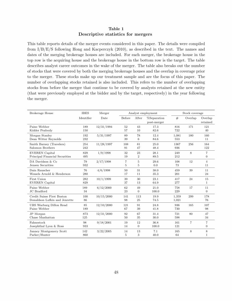

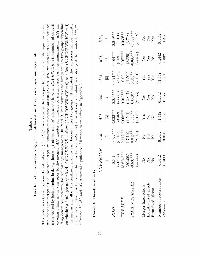
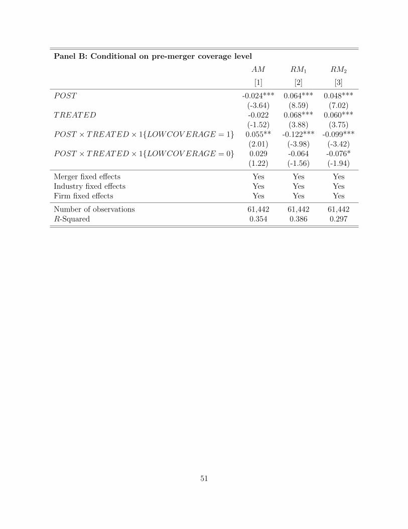
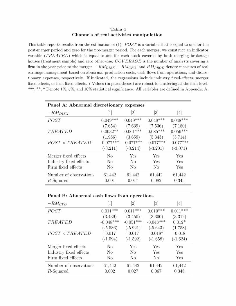
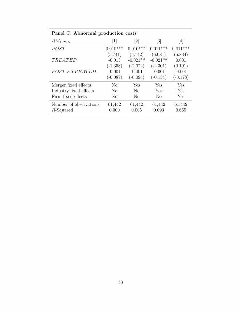
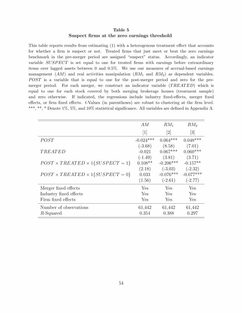
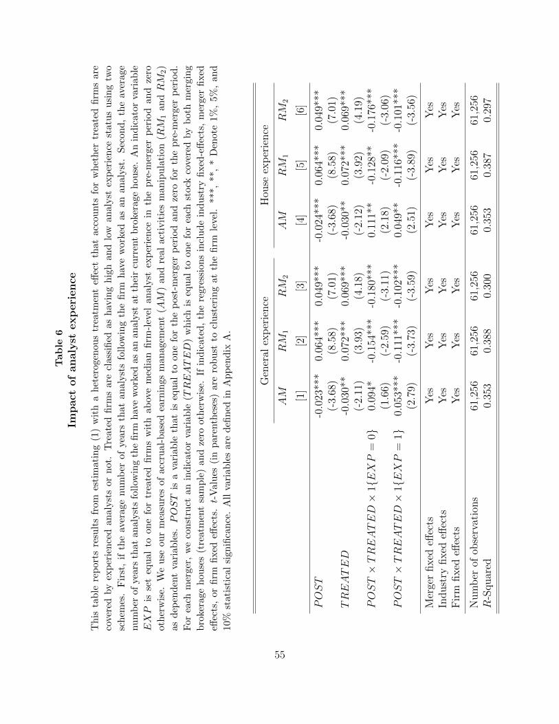
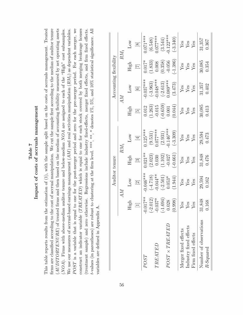
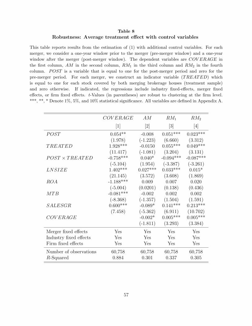
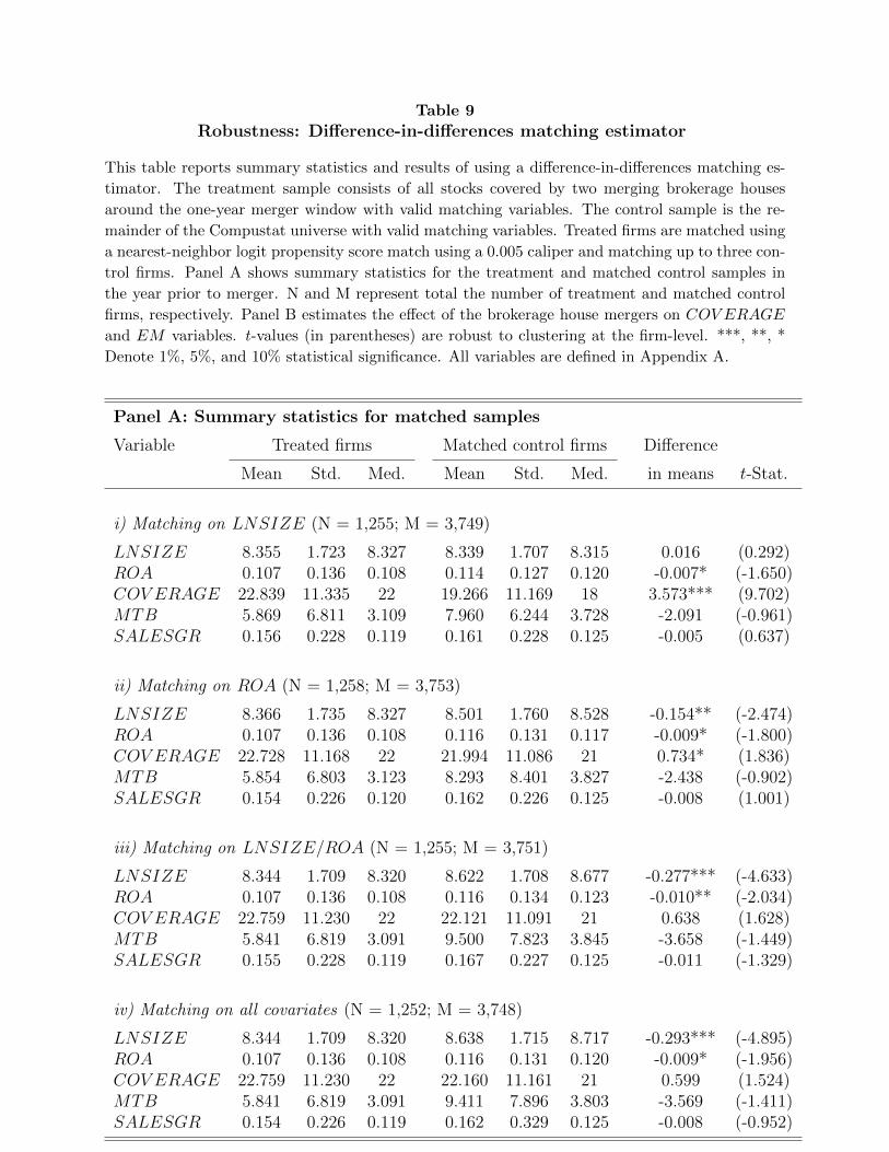
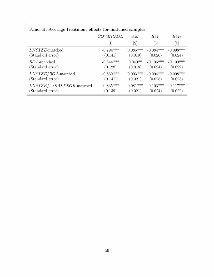
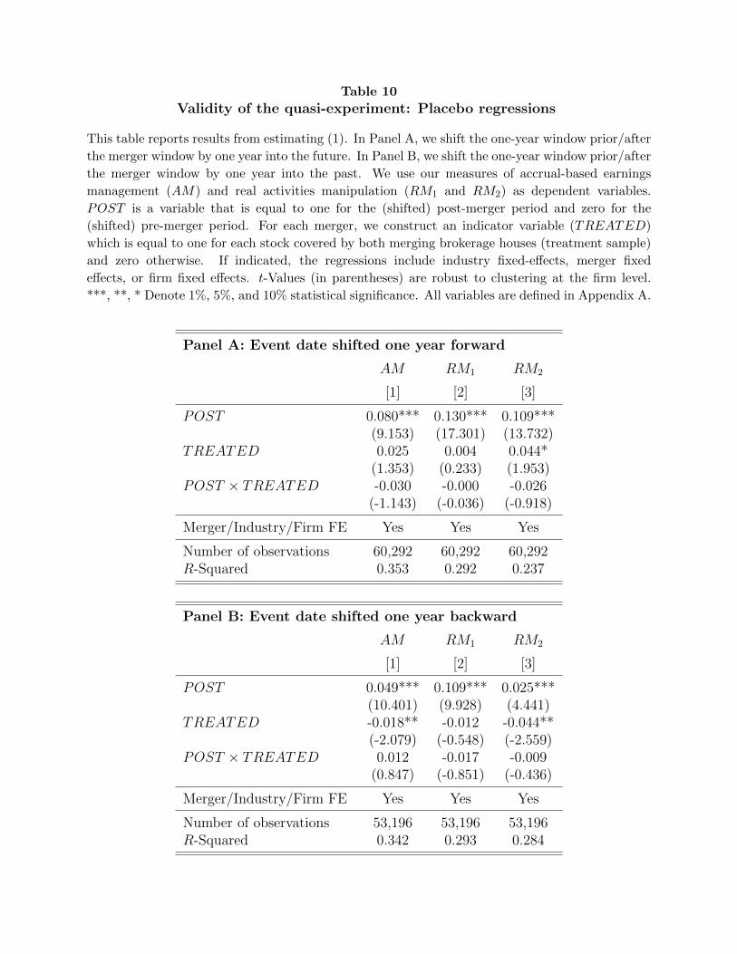
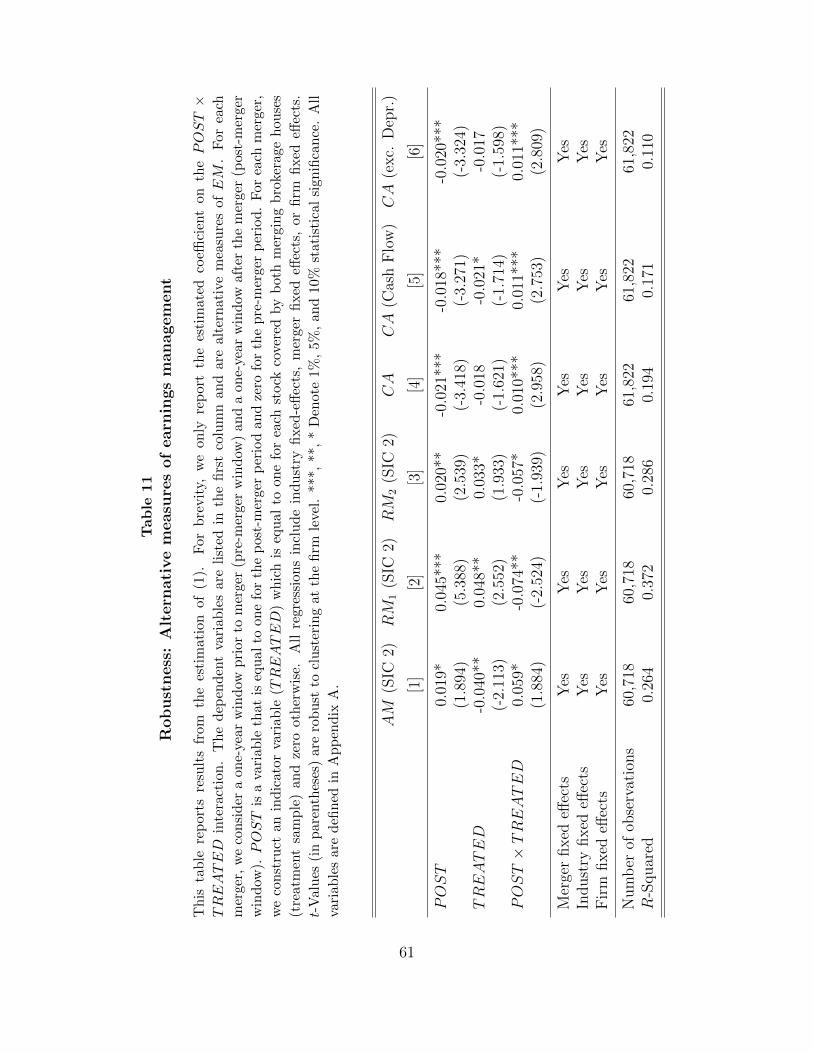
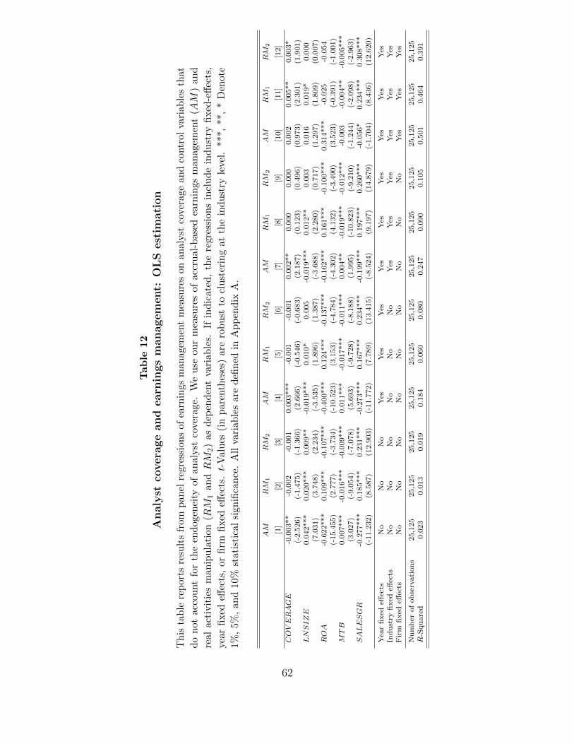


![FINNES DET EN OFFENTLIG LEDELSESMODELL? · Choice-teori [Niskanen] Transaksjons- kostnads- teori [Coase] Prinsipal- agentteori [Jensen & Meckling] Byråkrati- teori [Weber] Fra stat](https://static.documents.pub/doc/80x56/60990702ba2e7d663601d89e/finnes-det-en-offentlig-ledelsesmodell-choice-teori-niskanen-transaksjons-kostnads-.jpg)


