Analysts Consensus Fixation and Corporate Investment

First Draft: September 15, 2006

This Draft: May 25, 2007

Sébastien Michenaud*

Abstract

This paper empirically investigates whether executives alter capital budgeting decisions to

meet or exceed analysts’ earnings per share (EPS) consensus forecasts. I find that firms increase

their likelihood to meet or beat analyst EPS consensus forecasts by reducing investment. A

reduction in investment creates positive earnings surprises through a reduction in depreciation costs

and collateral cash expenses. Furthermore, firms reduce investment when analyst pressure is high at

the start of the year (as measured by abnormally high consensus forecasts early in the year). Firms

with better investment opportunities are more inclined to reduce investment to create earnings

surprises and tend to reduce more investment as a response to analyst pressure. In addition, firms

with lower managers’ entrenchment are also more inclined to reduce investment to create earnings

surprises. This pattern is consistent with underinvestment in response to analyst pressure, a

behavior that is harmful to shareholders’ interests. Taken together these pieces of empirical

evidence point to the harmful pressure exerted by the analysts’ forecasting activity on capital

budgeting decisions.

* HEC School of Management, Paris, 1 rue Libération, 78351 Jouy en Josas, Cedex, France, and Swiss

Finance Institute-FINRISK, University of Lugano, Via G. Buffi 13, 6904 Lugano, Switzerland.

Email: michenauds@hec.fr.

I would like to thank François Degeorge, Thierry Foucault, Francesco Franzoni, Ulrich Hege, Frédéric

Palomino and David Thesmar for helpful discussions and suggestions. All errors are my own. Financial

support from FINRISK is gratefully acknowledged.

1

1 Introduction

Analysts have often been accused of exerting excessive harmful short-term pressure on

managers in the United States. Several empirical studies have confirmed the propensity of U.S.

companies to misrepresent financial information to meet or exceed earnings thresholds. For

example, Degeorge, Patel and Zeckhauser (1999) document that the distribution of earnings forecast

errors exhibit patterns strongly suggestive of earnings management to reach earnings targets set by

analysts. Jensen and Fuller (2002) argue that the “earnings game” in which managers are stuck

may represent important real costs for the firm that go beyond the misrepresentation costs induced

by pure accounting earnings management. Managers may take business decisions for the sake of

meeting or exceeding aggressive, sometimes unrealistic, analyst expectations. This conjecture is

somewhat difficult to observe empirically, as we cannot observe the valuable investment projects

that have not been pursued by companies as a result of this supposed adverse pressure. But Graham,

Harvey and Rajgopal (2005) provide evidence, in a survey of U.S. CFOs, that managers are actually

acting as suggested by Jensen and Fuller. Among other things, they find that 55% of the U.S. CFOs

declare themselves quite ready to destroy firm value, by reducing investment in positive NPV

projects, in the hope of reaching their desired earnings targets.

I build on this previous work and examine the consequences of earnings management for

corporate investment. I propose to empirically investigate whether managers alter corporate

budgeting decisions to meet or beat analysts’ consensus earnings per share (EPS) forecasts.

This work rests on two main assumption building blocks. I first posit that corporate investments

may have a direct impact on a firm’s earnings. Postponing or canceling certain corporate

investments may mechanically reduce expenses in the income statement, and result in higher

earnings relative to what they would have been, had the investment gone through. Consider a firm

that plans to start new operations. Such an investment is usually associated with a ramp up phase

during which associated costs - e.g. personnel, advertising, rental and depreciation costs - that

appear in the income statements need to be incurred, while revenues generated from the project will

materialize in later periods. Investing in this project may actually jeopardize the meeting of

analysts’ EPS forecasts for the period considered, and probably also for later periods, as earnings

will be hurt. If meeting financial analysts’ consensus forecasts is important to the CEO, and analysts

cannot be tamed to revise their consensus downwards, he may well be tempted to either postpone

the investment to a later period, or to cancel it altogether. Investment will mechanically reduce net

income through depreciation costs. Indeed, depreciation is an accounting item that is directly

impacted by an increase in investment. I actually find that the economic impact of reducing

corporate investment on net income through the depreciation channel is quite large: a reduction in

investment by one (within-firm) standard deviation results in an estimated increase of 50% in mean

2

net income. In addition, using quarterly data on my sample of firms, I find that investing in one

quarter increases Selling General and Administrative Expenses (SG&A) beyond the increase in

depreciation the following quarter, suggesting that corporate investment generates additional

expenses in the income statement that could potentially act as an impediment to reaching earnings

targets.

Second, I assume that earnings are an important metric to managers, and that they care about

them. Graham, Harvey and Rajgopal (2005) report that CFOs overwhelmingly consider EPS as the

most important metric for firm performance, despite the strong emphasis of cash flow in the

academic finance literature. Meeting or exceeding certain EPS thresholds is considered very

important by managers, because not doing so is perceived as being strongly penalized in the stock

market. Skinner and Sloan (2002) and Kinney, Burgstahler and Martin (2002) show small negative

earnings surprises are associated with significant negative stock price reactions.

Based on these assumptions, I test the hypotheses that (i) firms reduce investment to increase

their probability of meeting or beating the analysts’ earnings consensus forecast and (ii) firms that

face excessive pressure to attain analysts EPS forecasts reduce their investment. While hypothesis

(i) is straightforward to test, notwithstanding potential endogeneity issues, I need some measure of

the excessive pressure exerted by analysts on management early in the year to test hypothesis (ii). I

build a proxy that is a measure of the abnormal level of EPS expected growth for the year relative to

last year’s realized EPS. It is constructed in two steps. I first measure the consensus analysts

forecast growth in EPS relative to last year’s realized EPS. I then regress this measure against past

firm’s performance and characteristics, and consider the residual as the abnormal level of analyst

forecast EPS expected growth.

I use an unbalanced panel of U.S. firms covered by analysts over the period 1981-2005 built

from the merged CRSP-Compustat Industrial database and I/B/E/S and test two different

econometric specifications corresponding to the two hypotheses presented above. The first model is

a fixed effects logit model where a dummy for non-negative earnings surprises is regressed against

corporate investment and a number of standard controls in the earnings surprises literature. The

second specification is a capital investment model where investment is regressed against the proxy

for analyst pressure and a number of standard controls in the investment literature.

The results of this analysis support the above hypotheses, and are both statistically significant,

and economically important. Firms that reduce capital expenditures by one standard deviation

increase the probability of meeting or beating analysts’ consensus forecasts by twice as much as

when they increase accruals by one standard deviation. In the finance and accounting literature,

accruals management has been found to be the main variable through which managers are creating

earnings surprises (Brown (2001) and Burgstahler and Eames (2006)). In addition, firms that face

3

high analyst pressure at the start of the year decrease their investment by 0.1% to 0.2% of total

assets, a 2% to 3% decrease relative to median cross-sectional capital expenditures.

I also find that firms invest more in the year following earnings surprises, suggesting that the

reduction in investment enabling firms to exceed the consensus forecast is partially caused by

project postponement from one fiscal year to the next. Because of the time value of money, project

postponement will cause loss of value. Say cost of capital is 15%: the net present value of the

postponed growth opportunities is reduced by 15%, not a trivial amount.

The causality link between investment and earnings surprises in the logit specification is not

necessarily obvious because these two variables are determined during the same period. Our

specification could thus suffer from simultaneity bias. Two stories could explain the simultaneous

negative correlation between investment and earnings surprises. The first story argues that

investment decisions could be jointly determined by a shock that also affects analysts’ prediction

abilities in the same fiscal year. Analysts would be too pessimistic about firms experiencing a

negative shock that also negatively impacts investment decisions. This story is inconsistent with the

evidence in Elliott, Philbrick and Weidman (1995). These authors find that analysts actually

underreact to bad news occurring during the contemporaneous year. Positive earnings surprises

occur less often when firms experience a negative economic shock. Alternatively, another story

argues that CEOs deliberately engage in cost-cutting or restructuring plans. Such plans would

simultaneously result in investment reduction at the firm level. Analysts would be too pessimistic

about the positive effects on earnings of such plans, and positive earnings surprises would be easier

to achieve. Such story is inconsistent with the finding that analysts revise forecasts downwards after

restructuring news but remain too optimistic about future earnings (Chaney, Hogan and Jeter

(1999)). It actually becomes harder to create positive earnings surprises. As a result, simultaneity

biases should not be too much of an issue. However, to further rule out any concerns about the

direction of the causality between investment and earnings surprises, I use quarterly data from

I/B/E/S and Compustat, and find that meeting or beating consensus forecasts in the last quarter of a

fiscal year is negatively correlated with investments in previous periods. Earnings surprises for the

year are also negatively correlated with investment in the previous fiscal year. Thus, it appears that

investment decisions taken early in the fiscal year influence the outcome of meeting or beating

analysts’ consensus forecasts in later periods.

An interesting question is whether the reduction in investment induced by managers’ fixation

on consensus forecasts corresponds to a reduction of overinvestment (e.g. empire building, pet

projects), or the passing up of valuable investment opportunities. To address this question, I use two

different approaches.

4

First, I run regressions on portfolios of firms ranked by their governance index. Firms with

good governance are expected to suffer less from overinvestment than firms with bad governance

(Jensen, 1986) because managers’ monitoring by shareholders and the board should be tighter. The

managers of these firms are also typically less entrenched, so they should be more prone to be fired

after bad firm performance (Fisman, Khurana and Rhodes-Kropf (2004)). The results suggest that

the decreased investment related to EPS consensus beating is not more pronounced for firms that

have lower quality governance charters. On the contrary, firms ranked by a manager’s entrenchment

index (Bebchuk, Cohen and Ferrell (2004)) or the Gompers, Ishii and Metrick (2003) governance

index only display a significant negative effect of investment for the good governance firms. This

suggests that the short-term pressure created by the analysts’ forecasting activity induces managers

to invest less to avoid negative earnings surprises. By doing so, they also reduce the risk of being

ousted by shareholders unhappy about the firm’s stock price performance.

Second, I sort firms by the size of their investment opportunity set, as proxied by their Tobin’s

Q. If the reduction in investment related to earnings surprise or related to analyst pressure occurs

because it purges excess investment, it should be stronger for firms with low investment

opportunities (those are firms for which, for a given level of investment, the percentage of

investment that is excessive is higher). It turns out that firms with average to good investment

opportunities tend to decrease more their investment to beat consensus forecasts than firms with bad

investment opportunities. This is also consistent with findings by Degeorge, Patel and Zeckauser

(2007) who show that glamour firms worry more about missing the consensus as they have more to

lose. These patterns are consistent with underinvestment in response to analyst pressure: firms

cancel or postpone good projects to avoid negative earnings surprises.

This work contributes to the literature in several respects. First, it adds to the large existing

earnings surprises literature by pointing to a new variable through which managers create non-

negative earnings surprises. The literature had previously identified accruals management (Brown,

2001 and Burgstahler and Eames, 2006) and forecasts management (Matsumoto, 2002 and

Burgstahler and Eames, 2006) as the main levers through which CEOs create non-negative earnings

surprises. Investment in fixed assets had never been considered previously. This is an important

finding, as changes in investment affect the firm’s real activities, as opposed to accounting

manipulations. It suggests that the analysts’ forecasting activity represents an important factor in

corporate financial decisions. Second, this work adds to the fairly recent corporate finance literature

linking financial analysts’ coverage with firms’ corporate finance decisions. Chang, Dasgupta and

Hilary (2006) and Doukas, Kim and Pantzalis (2006) studied the analysts’ coverage influence on

financing and investment decisions, while Li and Zhao (2006) worked on the analysts’ impact on

dividend policy. These studies concluded that analysts reduce information asymmetry between

5

managers and the stock market. These findings suggest that analysts have a beneficial influence on

corporate financial policies in the sense that they impose less financial constraints on firms, be it

costs of equity issuance or costly dividend signaling. On the other hand, Doukas et al. (2006) also

argue that reduced financing constraints owed to abnormal excess analyst coverage result in

overinvestment and subsequent low excess returns. In contrast with these findings, I find that

analysts exert adverse short-term pressure on the firms’ capital budgeting decisions, and that they

induce underinvestment rather than overinvestment in the short term. Finally, this work supports the

findings by Graham, Harvey and Rajgopal (2005) in a survey of 400 U.S. CFOs, where managers

recognized they might reduce investment to meet their desired earnings benchmarks. It suggests

that the “beliefs” described by CFOs in this survey are actually in the works in the U.S. stock

market. Managers do succeed in creating earnings surprises when they reduce investment.

The paper is organized as follows: section 2 develops the main working hypotheses; section 3

presents the empirical strategy while section 4 briefly describes the data. Section 5 presents the

main empirical results while section 6 presents robustness checks and section 7 concludes.

2 Hypothesis development

I posit that corporate investments may have a direct impact on a firm’s earnings, and that

managers, who care about earnings and the target set by the analyst EPS consensus forecast, adjust

their investment policy to meet or exceed this target.

The main hypotheses of this work are based on two main arguments.

I first assume that corporate investment has a direct impact on a firm’s earnings. There are two

reasons why this assumption holds true. The first and most straightforward reason is that corporate

investment directly impacts depreciation expenses. Depreciation is a non-cash cost that depends

directly on the level of past and contemporaneous investment in fixed assets. Capitalized fixed

assets that have not been fully depreciated still generate depreciation expenses up until the end of

their depreciation period, their assumed useful economic life. This is based on usual accounting

conventions for each class of asset. New additions in fixed assets during the year, capital

expenditures for the year, generate depreciation expenses in the same fiscal year. The influence of

corporate investment on depreciation expenses depends on several factors, like the depreciation

method that is used (straight-line, or accelerated depreciation), the class of fixed assets that have

been acquired, and various other exemptions and options left at the discretion of managers. Section

5.2 empirically investigates the economic impact that such a direct effect has on net income. The

depreciation effect on earnings appears to be quite large and significant.

In addition, I argue that the influence of corporate investment on net income goes beyond this

direct channel. Indeed, postponing or canceling certain corporate investments may reduce, although

6

with some lag, other expenses in the income statement and result in higher earnings. Consider a

firm that plans to start new operations, e.g. a plant or a retail store. Such an investment is usually

associated with a ramp up phase during which costs that appear in the income statements need to be

incurred. Workers of the plant or store will be hired and trained, some of the equipment and

property required for the project may be leased, not purchased, so additional expenses that are

directly associated with the project will appear in the income statement. In addition, advertising

expenses may be incurred to promote the new products manufactured or the retail store. The

following excerpt from the 2006 annual Apple 10K report illustrates the above discussion. In this

example, an increase in capital expenditures related to an aggressive strategy of retail stores

development leads to a series of additional costs that the company needs to incur

contemporaneously.

“Through September 30, 2006, the Company had opened 165 retail stores. The Company’s

retail initiative has required substantial investment in equipment and leasehold

improvements, information systems, inventory, and personnel.”

“[…] a relatively high proportion of the Retail segment’s costs are fixed because of

personnel costs, depreciation of store construction costs, and lease expense.”

Apple 10K report, September 2006

Based on the above discussion, it appears that investment in fixed assets will generate several

collateral cash expenses: labor, advertising, leases expenses.

On the other hand, revenues generated from the plant or store will materialize in later periods.

As a result, investing in such a project could jeopardize the meeting of financial analysts’ EPS

forecasts for the period considered, and probably also for later periods. Indeed, launching such a

project will lead to immediate additional costs that appear in the income statement, and to revenues

that will not materialize immediately. If meeting financial analysts’ consensus forecasts is important

to the CEO, and the CEO cannot manage analysts’ expectations downwards, he may well be

tempted to either postpone the investment to a later period, or to cancel it altogether. This

postponement decision will have a negative impact on the firm’s value because investment

opportunities have been abandoned to competitors for some time. More importantly, because of the

time value of money, such a decision destroys value to shareholders. The assumption described in

this example is supported by findings from Graham, Harvey and Rajgopal (2005) in a survey of 400

U.S. firms’ financial executives. The authors find that 55% of the interviewed CFOs state they are

ready to “delay starting a new project even if it entails a small sacrifice in value” to meet the desired

short-term earnings target.

The second assumption is that earnings are an important metric to managers, and that they care

about them. Graham, Harvey and Rajgopal (2005) report that CFOs overwhelmingly consider EPS

7

as the most important metric for firm performance, despite the strong emphasis of cash flow in the

academic literature. Meeting or exceeding certain EPS thresholds is considered very important by

managers, because not doing so would be strongly penalized in the stock market. Skinner and Sloan

(2002) show that growth firms that fail to meet earnings benchmarks such as analysts’ forecasts

suffer large negative price reactions on the reporting date. Graham, Harvey and Rajgopal (2005)

also report that CFOs believe that meeting such earnings benchmarks helps build the credibility

with the stock market and the external reputation of the management.

As a result of these two assumptions, I hypothesize that managers will take investment

decisions that are influenced by their willingness to alter earnings outcomes. I am particularly

interested in analysts’ earnings forecasts outcomes for two reasons. First, analysts’ consensus

forecasts are a pure collective construct from the financial analysts community. They are therefore

an ideal variable against which one can measure the influence of analysts on the managers’

decisions. Second, these forecasts have been shown in the literature to be important benchmarks

that are targeted by managers (Degeorge, Patel Zeckhauser (1999)) and the earnings surprises are

influenced by discretionary expenses and accruals management (Brown (2001) and Burgstahler and

Eames (2006)) and analysts’ expectations management (Matsumoto (2002)). Results from a survey

of CFOs by Graham, Harvey and Rajgopal (2005) confirm these earnings management practices are

widespread. They also suggest that managers postpone investment to create positive earnings

surprises. If, as suggested by these authors, managers postpone investment to create positive

earnings surprises, we would expect lower investment to increase the probability of positive

earnings surprises in the same fiscal year, and higher investment in the year following past positive

earnings surprises.

Based on these assumptions and findings, I test the following two hypotheses:

Hypothesis H1: Firms reduce investment to meet or beat analysts’ EPS consensus forecasts.

Hypothesis H2: Firms’ reduction in investment to beat EPS forecasts is temporary: the investment

will be higher following past positive earnings surprises.

Notice that there are several reasons why hypothesis H1 could be difficult to identify in the

data.

First, there is a lot of information asymmetry between the manager and the firm’s outsiders

concerning capital budgeting decisions: as a firm outsider, the researcher cannot observe the firm’s

investment opportunity set and the planned timing of such projects. This is an important benefit to

the manager, because, contrary to earnings manipulation that can be identified through careful

analysis of financial statements, an investment project cancellation or postponement could easily be

unnoticed by the firm’s outsiders, unless it is large enough.

8

Second, managers have a wide array of less costly instruments at their disposal to create

positive earnings surprises. We know from Matsumoto (2002) and Burgstahler and Eames (2006)

that managers use both earnings management and analysts’ expectations management to create

positive earnings surprises. Earnings management is carried out through accruals management.

Managers increase the non-cash component of earnings to increase EPS and meet or beat EPS

forecasts and other earnings thresholds. Such a manipulation is costly because managers will have

to decrease the non-cash components of earnings in the future to make up for past increases, and

because such an action is potentially visible to the careful investor. Managers will also significantly

increase the probability to create positive earnings surprises by guiding analysts’ forecasts

downwards. Doing so will make analysts’ consensus forecasts easier to attain. Forecast

management will be costly because managers will exert effort in convincing analysts that their

forecast are too high, and because the induced downwards forecast revisions may have a negative

impact on stock prices in the short term. However, earnings management and earnings guidance

cause significantly lower firm value destruction than project postponement or cancellation, because,

for the most part, they only involve accounting and expectations manipulations, and as such, they

should not influence too much real firm activities1. Firms are therefore expected to resort less to

investment reduction than earnings or expectations management to create positive earnings

surprises.

All the above arguments go against finding a significant effect of investment on positive

earnings surprises in the data. They suggest it is important to select a precise enough econometric

specification to identify the hypothesized effects.

In addition to the added difficulty in identifying hypothesis H1, the above discussion also

suggests that those firms that face high pressure from analysts early in the year will also be more

likely to reduce investment. I implicitly assume here that firms under high analyst pressure will find

it hard to avoid negative earnings surprises through the sole use of earnings management and

expectations management. Furthermore, in order to increase EPS through investment reduction,

managers need to plan such an investment reduction sufficiently ahead of time. I expect managers

to respond to early signals sent by analysts that current fiscal year EPS forecasts would be difficult

to achieve in the fiscal year without reducing investment, a costly decision.

Hypothesis H3: Firms under high analyst pressure will reduce investment.

Firms that face high analyst pressure will typically be firms that start the fiscal year with an

analysts’ EPS consensus forecast for the current year that is excessively high. I will define more

precisely what I mean by “excessively high” later on.

1 Roychowdhury (2006) provides an indirect evidence of earnings management through real activities (e.g. sales at

discount prices to boost EPS). In this case, earnings management destroys value to shareholders and involves more than

misrepresentation costs due to accruals management.

9

3 Empirical Strategy

To test hypothesis H1, I use a panel logit specification, where a dummy variable for meeting or

beating the analysts’ consensus forecast is regressed against corporate investment and various

standard control variables used in the literature. I take advantage of the dataset’s panel structure to

control for the unobserved time invariant firm heterogeneity, running all logit regressions with firm

fixed effects. I also add year fixed effects to control for time variant unobserved heterogeneity.

Wooldridge (2002, p. 491) argues that the logit panel regression with fixed effects is the least

restrictive specification for binary response models with panel data. It does not make any

assumption about the relationship between the unobserved heterogeneity and the independent

variables, contrary to random effects specifications2. Therefore I use the logit fixed effects model.

This choice is further justified by the results of a Hausman (1978) specification test that strongly

rejects the logit with random-effects model against the logit with fixed-effects model with a

significance level of 0.01%. The estimated coefficients are therefore within-firm effects. The

baseline equation for this specification is presented below:

Pr(Above EPS consensus forecastit = 1) = F( t + i+ . Capital expendituresit+ .CONTROLSit 1+ it )

F( X) =e X

1+ e X (1)

where F(.) is the logistic cumulative distribution function, is the column coefficient vector and X

is the sample observations matrix. If hypothesis H1 is verified, the coefficient on will be negative.

One could be concerned about simultaneity bias because Above EPS consensus forecast and

Capital expenditures are determined over the same period. Non-negative earnings surprises may be

jointly determined by an unobserved factor. Two different stories would be consistent with this

potential issue.

First, investment decisions could be jointly determined by a shock that also affects analysts’

prediction abilities in the same fiscal year. In this story, analysts are too pessimistic about firms that

experience a negative shock that negatively impacts investment decisions. This story is in

contradiction with the empirical evidence by Easterwood and Nutt (1999) and Elliott, Philbrick and

Weidman (1995). The former authors find that analysts underreact to bad news and overreact to

good news contained in the prior year’s performance. The latter authors find that analysts

2 I do not use probit panel regressions with fixed effects because they suffer from inconsistent parameters estimation

(Wooldridge (2002), p.484). Probit panel regressions with random effects suffer from the assumption of independence

between the unobserved effects and independent variables and the normality assumption on the unobserved effects, a

“strong assumption” according to Wooldridge (2002, p.485).

10

underreact to bad and good news within the forecast year. This empirical evidence is consistent

with bad news being associated with less positive earnings surprises, a story that is inconsistent

with reduced investment being associated with positive earnings surprises. Nevertheless, to further

rule out any concerns about this issue, I control for past operating performance and analysts’

forecasts revisions within the fiscal year in some of the model specifications.

Alternatively, investment decisions could be jointly determined by a shock that also affects the

firms’ earnings in the same fiscal year. In this story, firms reduce costs and increase the probability

of positive earnings surprises at the same time as they reduce capital expenditures. Note that if this

shock was exogenous, this story would be in contradiction with a neoclassical theory argument: if

costs go down due to an exogenous shock, investment opportunities should increase and so the firm

should invest more, not less. However, it could be that managers decide to reduce expenses and

investment in the same period, e.g. for restructuring purposes. Unfortunately, controlling for such

decision is difficult because our working assumptions confound the effects of investment and cost

reduction. According to hypothesis H1, I expect costs to be reduced, some of these costs with a lag,

as capital expenditures are reduced. One way to disentangle the two effects will be to use lagged

capital expenditures relative to earnings surprises. There should be no reason that a simultaneous

shock on capital expenditures and costs in earlier periods creates positive earnings surprises in later

periods, unless analysts overreact to restructuring news, anticipating too large reductions in costs. In

fact, Chaney, Hogan and Jeter (1999) find that firms announcing restructuring charges are also less

likely to create positive earnings surprises. Although analysts revise downwards their EPS

forecasts, they underreact to the restructuring news. As a result, one should not be too concerned

about the simultaneity of earnings surprises and lower investment due to the same restructuring

decisions.

Based on the above discussion, endogeneity problems should not be too much of a concern.

Nevertheless, to further strengthen results about the direction of causality, I use quarterly data from

I/B/E/S and Compustat to control for the timing of the investment decision relative to its effects on

earnings surprises. I then estimate the following model:

Pr(Above Q4 EPS consensus forecastit = 1) = F( t + i+ . Q(4 -k)Capital expendituresit+ .CONTROLSit 1+ it )

F( X) =e X

1+ e X (2)

where Above Q4 EPS consensus forecastit is a dummy variable for meeting or beating the analysts’

consensus forecast for the last quarter of the fiscal year t, and Q(4 - k) Capital Expenditures is

11

capital expenditures in quarter 4-k, with 1 k 3 (I use capital expenditures from one the first three

quarters). In addition, I also test specifications where the same dummy variable is regressed against

capital expenditures in the first half of the year (the sum of capital expenditures in the first two

quarters of the year). I further test another specification where Above EPS consensus forecastit is

regressed against Capital expenditures in the previous year. We will see that the results from model

(1) remain robust to these new specifications.

To test hypothesis H3, I use standard investment specification equations on unbalanced panels

and regress Capital expenditures against Analyst pressure and standard controls in the investment

literature. I also use firm fixed effects as in previous corporate investment studies (Baker, Stein and

Wurgler (2003) and Chen, Goldstein and Jiang (2006)). Year fixed effects are also added to the

specification. The corresponding baseline equation is as follows:

Capital expendituresit = t + i + . Analyst pressureit + .CONTROLSit 1 + it (3)

This empirical strategy allows me to measure the effects of Analyst pressure early in the year

on the investment policy for the same fiscal year. Notice that, because Analyst pressure is measured

early in year t while investment decisions are taken throughout the same fiscal year, the direction of

causality appears clearly from the model.

Finally, to test hypothesis H2, I look at the effects of having met or beaten analysts’ forecasts in

the previous year on investment for the current year. I use standard investment specification

equations on unbalanced panels and regress Capital expenditures against Above EPS consensus

forecasts in the previous year. The equation is identical to equation (2) except for the variable of

interest, Above EPS consensus forecasts:

Capital expendituresit = t + i + . AboveEPS forecastsit 1 + .CONTROLSit 1 + it (4)

4 Data

I construct the dataset from three main sources. The sample consists of U.S. firms listed in the

merged Center for Research on Security Prices (CRSP) - Compustat Industrial Annual database at

any point in time between 1981 and 2005. I also use the CRSP – Compustat Industrial Quarterly

database that I merge with the main database to obtain quarterly data for all firm-fiscal year

observations, when available. I exclude financial services firms (SIC code 6000-6900), regulated

utilities (SIC code 4900), firms with book values smaller than $10 million and firms with no analyst

coverage (i.e. not present in the I/B/E/S Historical Summary Files). I winsorize all variables except

Firm Age and Analysts at the first and ninety-ninth percentile. This helps mitigate the impact of

outliers and measurement errors in the data.

12

I obtain data on analyst coverage, EPS consensus forecasts, and EPS realizations from the

I/B/E/S Historical Summary Files. I use the I/B/E/S files that are unadjusted for stock splits: these

files are free of the important rounding errors first identified by Diether, Malloy and Scherbina

(2002) in the I/B/E/S adjusted files. These rounding errors resulted in important measurement errors

in the standard errors of analysts’ forecasts. They would also introduce measurement errors for

earnings surprises: firms may be wrongly classified as generating non-negative earnings surprises

when they are actually creating negative earnings surprises. The I/B/E/S files unadjusted for stock

splits require additional processing to properly account for stock splits between the date the

consensus EPS forecast is recorded and the EPS announcement date. I follow the procedure

recommended in WRDS by Robinson and Glushkov (2006) to adjust for stock splits from the

I/B/E/S unadjusted files. I also obtain governance index data from Andrew Metrick3 and

entrenchment index data from Lucian Bebchuk4.

The full sample includes 65,221 firm-year observations for an average of 2,609 observations

per year from 1981 to 2005. Before looking in details at the empirical strategy, I turn to the

construction of the main variables used in the baseline analysis.

Analysts’ Consensus Forecast

I construct the variable Above EPS consensus forecast as a dummy variable that is equal to 1 if

the firm’s EPS is larger than or equal to the analysts’ consensus forecasts and is equal to 0

otherwise. The baseline analysts’ consensus forecast is defined as follows. For each month before

the reporting of the actual EPS, the I/B/E/S Historical Summary Files provide a median of the

analysts’ EPS forecasts for the fiscal year. I use the latest median I/B/E/S EPS consensus forecasts

before the current fiscal year report date. This measure of the analysts’ EPS consensus forecast is

common in the literature. Other authors use the latest individual analysts’ EPS estimate before the

reporting of the EPS. As a robustness check, I use this alternative measure of EPS forecasts to

define my positive earnings surprise variable and find similar results.

Proxy for Analyst Pressure

I construct a proxy for the level of analyst pressure exerted on managers. To do so, I measure

the abnormal level of analysts’ expected increase in EPS relative to last year’s realized EPS. This

proxy measures whether managers face abnormally high or low EPS forecasts at the start of the

year. It is constructed in two steps. First, I compute the level of increase in EPS that is forecast by

analysts relative to last year’s realized EPS. This variable is measured early in the year after the

announcement date of last year’s EPS, so that analysts have updated their forecasts based on this

new piece of information. This measure, Forecast EPS change, is scaled by stock prices 90 to 120

3 http://finance.wharton.upenn.edu/~metrick/data.htm 4 http://www.law.harvard.edu/faculty/bebchuk/data.htm

13

days before last year’s EPS announcement. Stock prices are taken from I/B/E/S to ensure

consistency with the stock split adjustment process relative to EPS forecasts and EPS realizations.

Forecast EPS change = (EPS forecaststart of year t - actual EPSt-1)/Stock price t-1-90days

It turns out that Forecast EPS change is correlated with past firm’s performance and firm’s

characteristics. Analysts tend to be optimistic about firms that have had low past performance. They

predict higher EPS increase for firms that, in the previous year, had low Tobin’s Q, negative EPS,

low cash flow, large financial constraints, low analyst coverage, high forecast EPS increase in the

same industry (at the 3 digit SIC code level), small size, negative earnings surprises, and for which

analysts predict a turnaround (EPS is expected to be positive in the year and was negative last year).

To control for all these effects and introduce a measure of the abnormal level of analyst forecast

EPS increase, I regress Forecast EPS change against all these variables. The results are presented in

Table 1 in the appendix. This regression is a panel regression where the panel unit is the firm, and

year fixed effects are also included. The R squared of this regression is relatively high at 51%, thus

explaining a large portion of the variation in forecast EPS changes. That way, taking the residuals

of this regression, I obtain the within-firm Analyst Pressure variable that measures abnormal

pressure by analysts. By definition, Analyst Pressure is orthogonal to all the variables included in

the panel regression. It will be positive if the analysts’ forecast increase in EPS is too high relative

to past firm performance and characteristics. Managers will thus face abnormally high analyst

consensus EPS forecast at the start of the year in that case. Conversely, Analyst Pressure will be

negative if the analyst forecast increase in EPS is too low relative to past firm performance and

characteristics. Managers will thus face abnormally low analyst consensus EPS forecasts at the start

of the year in that case. I expect this proxy to be negatively correlated with investment, all else

being equal (Hypothesis H3).

[Insert table 1 about here]

Investment

I construct the main measure of corporate investment, Capital Expenditures, as capital

expenditures (Compustat item 128) scaled by beginning-of-the-year total assets (item 6)5.

It is important to stress that, if the hypothesis that CEOs reduce investment to meet earnings

forecasts is verified, they would like to hide this reduction in investment to the financial

community. They could do so by manipulating their accounts, so that they do not show that they are

investing less than what they should. Therefore, I should be particularly concerned about possible

accounting manipulations by CEOs to hide distortions in their capital budgeting decisions. To do

so, I only use a cash measure of investment that is less susceptible to accounting manipulations. I

exclude measures of investment such as capital expenditures plus research and development

5 All the results still hold when investment is measured as ratio of lagged gross property plant and equipment (item 7).

14

expenses, the baseline variable in Chen, Goldstein and Jiang (2006), because R&D is a noisier

variable of investment, for which managers have more accounting creativity leeway. R&D expenses

have been shown in the literature to be susceptible to accounting manipulation (see e.g. Bushee

1998), and much flexibility is left to managers to compute this expense. Likewise, measures such as

year-to-year changes in total assets are also excluded from the analysis because they include all

sorts of assets, including non-cash flow earnings components: accruals. As argued earlier, accruals

have been shown to be the main vehicle for earnings management: an increase in accruals is

positively correlated with firms meeting or beating analysts forecasts.

Controls

Based on previous studies on earnings surprises, I include several control variables in equation

(1) to control for accruals management, macroeconomic, industry and firm specific shocks, firm

past performance, firm size, firm risk, news arrival and uncertainty in the forecasting environment.

Accruals management has been shown to be an important variable through which firms create

earnings surprises (Brown, 2001, Burgstahler and Eames, 2006). The accounting literature on

earnings management has provided several methods to measure earnings management (Dechow et

al. 1995). Accruals represent the non-cash component of earnings. Earnings in year t are equal to

the sum of cash flows and accruals in the same year:

Earningst = Cash flowt + Accrualst

If managers have discretion in deciding the level of accruals for a given year, then we want to

measure the discretionary part of accruals. The simplest such proxy for discretionary accruals has

been provided by De Angelo (1986) who uses Changes in Total Accruals as a proxy for the

discretionary accounting adjustments6. Dechow et al. (1995) find that this measure efficiently

detects earnings management.

Changes in Total Accruals = Total accrualst - Total accrualst-1 = (DAt - DAt-1) – (NAt - NAt-1)

where DA is discretionary accruals and NA is normal accruals. If we assume that changes in normal

accruals are equal to zero on average, then changes in Total Accruals should reflect changes in

discretionary accruals. Following De Angelo (1986) and Dechow et al. (1995), I define Total

Accruals as follows: changes in current assets (item 4) minus changes in cash (item 1), minus

changes in current liabilities (item 5) plus current maturities of long term debt (item 44) plus

changes in income taxes payable (item 71) and I compute the difference between total accruals in

year t and total accruals in year t-1. There is one notable difference between my measure of total

accruals and the measure of accruals by the above authors. Because of the specific hypothesis I test,

I exclude depreciation expenses (item 14). Indeed, in my story, capital expenditures directly impact

6 For expositional clarity I rely on the simplest accruals management proxy. Using the more sophisticated modified

Jones (1991) model, following the procedure described in Dechow et al. (1995), provides similar results for all my tests.

15

depreciation expenses, and depreciation expenses will impact earnings to create earnings surprises.

Including depreciation expenses in the computation of Total Accruals could potentially reduce the

estimated effect of capital expenditures because of collinearity between these two variables7.

Prior research has documented that unexpected macroeconomic shocks affect earnings

surprises (O’Brien (1988)). Year-fixed effects provide control for general macroeconomic shocks. I

also include sales and cash flow to control for firm-specific shocks, and earnings surprises at the

industry level (at the 3 digit SIC code level) to control for industry shocks. Sales and Cash Flow are

respectively contemporaneous sales (item 12 in Compustat) scaled by lagged total assets (item 6),

and contemporaneous cash flow, computed as the sum of earnings before extraordinary items (item

18) and depreciation and amortization (item 14) scaled by start-of-year total assets (item 6).

Percentage above EPS forecasts in industry is the percentage of firms in the same industry that

created non-negative earnings surprises in the contemporaneous year, using the previously defined

variable Above EPS consensus forecasts.

We know from Degeorge, Patel and Zeckhauser (1999) that meeting or beating analysts’

expectations is less important for firms that incur losses. Therefore, I include a dummy variable for

firms that have posted positive EPS in the contemporaneous year.

Analysts underreact to bad news and overreact to good news in the prior year’s performance

according to Easterwood and Nutt (1999). Therefore, I include a control for firm past performance,

with Past profitability, defined as last year’s return on assets, (income before extraordinary items

(item 13) scaled by start-of-year Total Assets). Firms that had good past operating performance are

expected to create less positive earnings surprises while firms with bad past performance are

expected to create more positive earnings surprises. I also include a proxy for positive news arrival

by defining a dummy variable, Upwards consensus change, that is equal to 1 if the last analysts’

consensus forecast before EPS announcement is strictly larger than the first consensus forecast after

the previous fiscal year EPS announcement. Elliott, Philbrick and Weidman (1995) find that

analysts underreact to positive and negative news arriving during the forecasting period. As a result,

good news are positively associated with positive earnings surprises and bad news are associated

with negative earnings surprises.

Firms with high forecasting uncertainty are more likely to face analysts’ EPS consensus

forecast that are more easily attainable (Matsumoto, 2002). I include a control using the median

analyst consensus forecast standard deviation from the I/B/E/S Historical Unadjusted Summary

Files to avoid measurement errors (Diether, Malloy and Scherbina, 2002). Standard deviation of

forecasts is computed as the median of monthly EPS consensus forecasts standard deviation over

7 This modification is made purely on logical grounds. In practical terms, I find that the inclusion of depreciation in

Total Accruals computations does not reduce the significance of my results on Hypothesis H1, both for the De Angelo

(1986) model and for the modified Jones (1991) model presented in Dechow et al. (1995).

16

the fiscal year forecasting period. Analysts are also likely to forecast EPS with less accuracy for

young firms than for older firms, so I include a control for firm age, using a log transformation of

the number of years the company has been present in the Compustat Price Dividends and Earnings

database. In addition, in all the baseline regressions, I include analyst coverage to take into account

the total number of analysts issuing EPS forecasts in the year, and firm size to proxy for the public

information environment. Analysts follow more intensively large firms (Bhushan, 1989), and large

firms are generally considered to be the object of higher scrutiny by the investment community.

Earnings surprises may be more difficult to create for firms followed by a large number of analysts.

Indeed, Degeorge, Ding, Jeanjean and Stolowy (2005) and Yu (2006) show that high analyst

coverage reduces accruals management. I use a logarithm transformation of lagged Total Assets to

control for firm size.

Glamour firms are more likely to create earnings surprises than value firms because they may

have greater incentives to do so (Degeorge, Patel and Zeckhauser, 2007). To proxy value firms, I

use the ratio of tangible assets (item 7) to total assets.

Based on previous studies on corporate investment, I include several control variables in

equations (3) and (4) to control for investment opportunities, cash flow, analyst coverage, firm size,

financial constraints, firm risk, and the firm’s undervaluation.

In all of the investment equations, I include Tobin’s Q, a lagged market-to-book ratio, to

control for investment opportunities. Lagged market-to-book ratio is the market value of equity

(price times numbers of outstanding shares in Compustat, i.e. item 199 multiplied by item 25) plus

book value of assets minus the book value of equity (item 6 - item 60 - item 74 in Compustat)

scaled by the value of book assets (item 6), all values being measured at the end of the previous

year. In addition, following Fazzari, Hubbard and Petersen (1988) who argue that corporate

investment is sensitive to the availability of internal funds, I include contemporaneous cash flow

(Cash Flow) as control, where cash flow is the sum of earnings before extraordinary items (item 18)

and depreciation and amortization (item 14) scaled by start-of-year total assets.

Analyst coverage has been shown to positively influence equity issues and investment (Chang

et al., 2006 and Doukas et al., 2006). I define analyst coverage, Analysts, as the number of analysts

issuing a fiscal year t-1 EPS forecast for the firm in the I/B/E/S Historical Summary Files. I lag the

analyst coverage variable one period and use a logarithm transformation of raw analyst coverage in

all regressions.

In some of the investment equations, I include the firm’s future excess returns (Baker, Stein

and Wurgler (2003)’s undervaluation), the difference between the three year firm’s cumulative

stock return from year t+1 to year t+3 from CRSP and the stock market three year cumulative

return, as a control variable for stock price misvaluation. Baker and Wurgler (2002) and Baker,

17

Stein and Wurgler (2003) show that equity dependent firms invest more when their stock is

overvalued, as there is a negative relation between corporate investment and a firm’s future stock

return. I also follow these authors to construct a modified Kaplan and Zingales (1997) index of

financial constraints that excludes Tobin’s Q to avoid any spurious correlation in the specifications.

This variable is defined as follows:

Kaplan and Zingales (1997) index = -1.002 Cash Flow - 39.368 Dividends - 1.315Cash +

3.139 Leverage

All variables are lagged. Cash is defined as item 1 in Compustat scaled by lagged assets,

Leverage as the sum of long term debt (item 9) and the debt part of short term liabilities (item 34)

divided by the sum of debt and the value of book equity (item 9+item 34 + item 216). Dividends is

the sum of common stock dividends (item 21) and preferred stock dividends (item 19) scaled by

lagged assets. This index has been used extensively in the corporate investment literature (Baker,

Stein and Wurgler (2003), Chen, Goldstein and Jiang (2006)) and has been shown to capture the

effects of financial constraints in a world of costly external finance. Lower values of the index

capture low financial constraints firms (high cash flows, dividend payments, available cash and low

leverage) while higher values of the index stand for high financial constraints firms (high leverage,

low cash flows, dividend payments and cash in bank).

I also control for firm’s size using the logarithm of lagged Total Assets (item 6) as my baseline

measure. Additionally, I control for firm age where age is defined as the number of years a firm is

present in the Compustat Price Dividends and Earnings database to proxy for firm risk.

All the main variables are described in Table 2.

[Insert table 2 about here]

5 Corporate Investment and Earnings Surprises

5.1 Summary Statistics

Panel A of Table 3 reports the summary statistics for the whole sample of 65,221 firm-year

observations and for the two subsets of firms that met or exceeded analysts’ consensus forecast

during the year and firms that did not.

Firms that met or beat analyst forecasts are significantly larger, older, more profitable, have a

higher Tobin’s Q and larger contemporaneous cash flow. These firms are also less financially

constrained, as measured by the Kaplan and Zingales (1997) modified equity dependence index and

sell-side analysts more intensively cover them. They also managed their earnings upwards a lot

more, as testified by the positive mean change in total accruals. Firms that created non-negative

earnings surprises also invested more than firms that missed analysts’ consensus EPS forecasts.

While this finding is in contradiction with hypothesis H1, we should not be surprised about this

18

result. These firms have much larger Tobin’s Q and cash flow and are less financially constrained:

they are expected to invest more. Taken together, these results suggest that meeting or beating

analysts consensus forecast is associated with good news about the firm, and that not meeting these

forecasts contains somewhat bad news. Note that there is positive serial correlation for the variable

Above EPS consensus forecast between year t and year t+1 (0.16). Firms that outperform consensus

EPS forecasts in one year tend to repeat this performance in the following year.

Panel B of Table 3 presents correlation coefficients among the key variables of our analysis.

What is striking in this table is the positive and slightly significant correlation between Capital

expenditures and the dummy variable Above analysts’ EPS consensus forecast. Nevertheless, we

also notice a significant positive correlation with cash flows, past profitability and Tobin’s Q; and a

negative correlation with financial constraints. To be able to draw conclusions about the ceteris

paribus correlation between the earnings surprise variable and investment, we will need to

disentangle the effects of cash flows, investment opportunities and financial constraints. On the

other hand, Analyst pressure is significantly negatively correlated with Capital expenditures and

positive earnings surprises and positively correlated with contemporaneous cash flows. Firms that

face high analysts’ consensus forecasts will generate high cash flow but will invest less and be less

likely to create positive earnings surprises.

[Insert table 3 about here]

In Figure 1, we look at the time series of mean Capital expenditures and Tobin’s Q,

conditioning on the attainment of analysts forecasts at time t8. We get an interesting picture of the

firms’ investment pattern over time. Firms that are above analyst forecasts at time t had mean

investment ratios only slightly larger than firms that have not met analyst forecasts at time t.

However, as seen in Panel A of Figure 1, firms in this group have much better investment

opportunities, as proxied by their Tobin’s Q, they also have much larger contemporaneous cash

flow than firms not meeting analysts’ forecasts a time t, and as such, should invest much more.

What is striking in this graph is the slight investment reversal pattern for those firms that are

above expectations at time t. They invested less than the other group of firms between year t-3 and

year t, while they invest much more for the two following years and they invest more or less the

same in the following years. On the other hand, firms that have not met analysts’ forecasts show a

constant downward trend in investment that is only slightly more pronounced between year t and

t+19. This suggests that meeting or not analysts’ consensus forecast contains information about the

firms’ future prospects: firms that meet or beat analysts’ consensus forecasts tend to perform well

afterwards, while firms that did not tend to perform less well. This is confirmed by Panel A of

8 We also condition on the availability of the whole time series to avoid survival bias. 9 The average downwards trend in investment is owed to the decrease in investment from 2001 onwards. The results of

our analysis are unaffected by using different time periods for the multivariate regressions.

19

Figure 1 that exhibits the evolution of lagged Tobin’s Q for the same cross section of firms that are

above analysts’ expectations or not at time t.

This investment pattern could be explained by bad past economic conditions followed by an

unforeseen economic recovery in the year in which the firm beats analyst forecasts. It could also

suggest that earnings surprises occur in industries at certain points in time of the economic cycles.

Firms in industries that recover from previous sluggish market conditions could create non-negative

earnings surprises. Therefore, when we perform the multivariate analysis, we will need to take into

account such plausible explanations for this investment pattern.

Another possible explanation is based on the story that managers reduce investment to meet or

beat analysts’ consensus forecasts. Managers would be planning earnings surprises ahead by

reducing investment, and, afterwards, they would catch up postponed investments. This casual

observation from the graphs will be confirmed in the multivariate analysis when I control for

various factors, among which industry and past economic performance.

[Insert figure 1 about here]

I now turn to the presentation of evidence that corporate investment influences the firm’s cost

structure as postulated in the development of my hypotheses, and analyze its economic significance.

5.2 Corporate Investment and Cost Structure

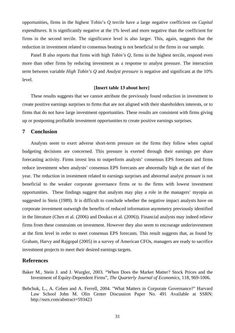
To get an idea of the economic importance that a reduction in corporate investment would have

on net income through the depreciation channel, it is useful to measure the average impact of a

year-over-year change in capital expenditures on the contemporaneous year-over-year change in

depreciation and amortization. To do so, I run panel regressions with firm fixed effects where the

dependent variable, the first difference in depreciation scaled by lagged total assets, is regressed

against the first difference in capital expenditures scaled by lagged total assets10. The first column

in Panel A of Table 4 presents the results of this regression. Results indicate that a 1% increase in

capital expenditures in year t results in a 0.066% increase in depreciation in the same year (all

variables are expressed as a percentage of total assets). On the other hand, in the second column of

the table, we observe that a 1% increase in depreciation decreases net income by approximately 1%

of total asset. Taken together, these results indicate that a reduction in the first difference in

investment by one (within-firm) standard deviation (6.87%) would result in an estimated increase of

50% in mean net income (6.87%*0.066*(-1.07)/0.98%), or an increase of 11% in median net

income (6.87%*0.066*(-1.07)/4.5%). So, it appears that the direct effects of corporate investment

on net income are economically large.

10 Year fixed effects are also included in the regression to control for time variant firm heterogeneity.

20

However, as argued in section 2, I also argue that the influence of corporate investment goes

beyond this direct channel. Empirical support for the above assumptions is mixed on annual data

and more convincing on quarterly data. Panel B of Table 4 exhibits correlation coefficients between

capital expenditures, Selling General and Administrative (SG&A), depreciation, rental, advertising

and labor expenses on annual data for my sample of firms. Both contemporaneous and lagged

capital expenditures are significantly correlated with depreciation, and rental expenses, but not with

advertising expenses or labor expenses, and they are negatively correlated with SG&A.

I also use quarterly accounting data from the Compustat Quarterly Industrial database. This

database does not provide a detail of SG&A expenses, but it allows me to analyze the impact of

Lagged quarterly capital expenditures on Quarterly SG&A expenses beyond its impact on

Quarterly depreciation and amortization expenses. Panel C of Table 4 presents results of the panel

regression with firm and quarter-year fixed effects where quarterly SG&A expenses is regressed on

quarterly depreciation expenses and lagged quarterly capital expenditures plus a control for the

common scaling factor, the inverse of total assets. This regression suggests that lagged quarterly

capital expenditures are positively correlated with quarterly SG&A beyond their influence on

depreciation expenses. However, these results should be interpreted with caution, as they could be

driven by an unobserved factor that would simultaneously influence investment and SG&A

expenses. For instance, a managerial decision to “cut all costs”, including investment could be

driving these results, e.g. for restructuring purposes.

Note, however, that the depreciation channel is important enough in magnitude to potentially

explain the effect of investment on earnings surprises.

[Insert table 4 about here]

5.3 Investment Reduction Hypothesis

I now move to the estimation and analysis of specification (1) presented in section 3, the main

specification. I test whether meeting or beating analysts’ consensus forecasts occurs more often or

less often the higher or the lower the investment at the firm level. According to hypothesis H1, I

expect to find a negative correlation between corporate investment and the probability to create

positive earnings surprises.

The results of these tests are presented in Table 5. The number of firm-year observations is

reduced relative to our full sample because the logit regression with fixed effects does not use

observations where the dependent variable for the firm observations, Above analysts’ EPS

consensus forecasts, are either all equal to 0 or all equal to 1. The reason being that these

observations, 5,279 observations for 2,296 firms, do not provide any estimation information11. They

11 For more on this and an illustrative example, see Wooldridge (2002) page 491.

21

are thus automatically rejected from the sample by traditional statistical software packages such as

STATA®. Column 1 presents the results for a simple specification where, in addition to Capital

expenditures, I add contemporaneous Sales, Cash flow, the logarithm transformation of Analysts

and of total Assets as controls. I also control for Past profitability and earnings management,

through variable Changes in total accruals. Column 2 adds controls for the average earnings

surprise level in the industry, Percentage EPS surprises in industry, Column 3 adds a control for the

dispersion of analysts forecasts, Standard deviation of forecasts, a control for firms that post

positive EPS at the end of the year, and for changes in consensus forecasts over the year. Column 4

introduces additional controls for firm risk, as proxied by the log transformation of firm age, and a

control for value firms, proxied by the ratio of tangible assets to total assets (Tangibles).

Columns 1 to 4 show that the coefficients on all the investment variables are negative and

significant at the 1% level. Investing more during the year decreases the likelihood of meeting or

beating analysts’ consensus forecasts.

The coefficients on contemporaneous Sales and Cash flow are positive and significant at the

1% level in all variants of the model. Sales provide a control for firm specific shocks in their ability

to generate revenue. On the other hand, contemporaneous Cash flow proxies for the firm’s ability to

generate high earnings per share, the object of the analysts’ forecasts. It also provides a control for

firm specific cash expenses shocks in the fiscal year as Sales already provide a control for revenues.

The coefficient on Past profitability is negative and highly significant. As suggested earlier in

our discussion of Figure 1, firms that recover from past economic difficulties find it easier to meet

or beat analysts’ consensus EPS forecasts. This result is also consistent with Easterwood and Nutt

(1999) who find that firms with low past performance create positive earnings surprises more often

in the subsequent year because analysts underreact to bad news and overreact to good news.

However, this past low performance is not what is driving the reduction in capital expenditures, as

testified by the negative coefficient on Capital expenditures.

Consistent with the literature on accounting manipulations, the coefficients on Changes in total

accruals are all positive and significant. The higher the increase in total accruals in the

contemporaneous year, i.e. the higher the increase in the non-cash component of net income, the

more likely the firm will meet or beat analysts’ consensus forecasts. Note however that the

significance is not very high in the last two models (columns 3 and 4) as the level drops to the 10%

and 5% level respectively12. Untabulated results show that the significance level is greatly increased

by the use of a random effects model or of a traditional logit model that does not take into account

the panel structure of the data, as previously carried out in the earnings surprise literature. However,

12 The use of modified Jones (1991) model to proxy for discretionary accruals management actually results in even

lower significance levels for the earnings management proxy: it no longer significantly increases the probability to meet

or beat analysts’ forecasts.

22

as discussed earlier, a Hausman (1978) specification test strongly rejects the random effects model

at the 0.0001 level against the fixed effects model.

Analyst coverage and firm size do not seem to strongly influence earnings surprises. Analyst

coverage is only significant in the first two specifications (columns 1 and 2) with the positive sign,

when a negative sign was expected, while firm size appears to have a negative significant

coefficient only in the last two specifications (columns 3 and 4). Consistent with Degeorge, Ding,

Jeanjean and Stolowy (2005) and Yu (2006), analyst coverage reduces earnings management, so the

negative effect of analyst coverage on earnings surprises should be captured by variable Changes in

total accruals.

As discussed previously, one could suspect that the patterns in the earnings surprises are related

to the overall earnings surprises in the same industry. Firms in the same industry could perform

better than expected by analysts because of unexpected changes in the industry economic cycle and

correlated forecasting errors at the industry level. More specifically, the decreased investment

would be correlated with earnings surprises because analysts forecast errors are correlated within

industries that experience a downturn. I control for this possibility by introducing variable

Percentage above EPS forecasts in industry, the proportion of firms in the same industry meeting or

exceeding analysts’ EPS expectations, where industry is defined at the 3 digit SIC code level. As

expected, the coefficient on this variable is positive and significant at the 1% level in all

specifications. Nevertheless, the introduction of this control does not reduce the significance of the

negative coefficient on Capital expenditures. On the contrary, the negative coefficient decreases

with the introduction of this control variable and its significance increases.

The negative correlation between Capital expenditures and earnings surprises is robust to the

introduction of additional controls. Indeed, Columns 3 and 4 show that higher dispersion in

analysts’ consensus forecasts, Standard deviation of forecasts, decreases the probability to create

positive earnings surprises. Firms with positive earnings per share have a higher likelihood of

beating forecasts, consistent with Degeorge, Patel and Zeckhauser (1999). Positive forecasts

changes are positively associated with earnings surprises. Analysts seem to underreact to positive

news about the firm that occur during the forecasting period. This result is consistent with the

results from Elliott, Philbrick and Weidman (1995) who show that analysts underreact to good

news. However, the introduction of this variable does not reduce the significance of the negative

coefficient on Capital expenditures. On the contrary, the significance is increased in column 3

relative to column 4.

Value firms create less positive earnings surprises than other firms, consistent with Degeorge,

Patel and Zeckhauser (2007).

23

The marginal effects of the last specification (presented in column 4) are presented for

reference. Nevertheless, as pointed out by Wooldridge (2002), any interpretation is subject to

caution. Indeed, fixed effects logit regressions do not estimate the fixed effects parameters. To

compute the marginal effect on the probability to meet or beat analysts’ consensus EPS forecasts,

one would need to get an estimate of the fixed effect for each firm. Therefore, I need to assume that

the fixed effects are equal to 0 and compute the marginal effects at the mean value of control

variables. The assumption that the fixed effects are zero on average is arbitrary because fixed

effects logit regression estimation does not impose any restriction on the mean value of fixed

effects. However, these marginal effects provide a rough estimation of the relative contribution of

each variable in the model on the probability to create non-negative earnings surprises. For

example, the marginal effect of a reduction by a one within-firm standard deviation in Capital

expenditures (-6.46%*-0.178=1.15%) is approximately twice as large as the marginal effect of a

one-within-firm standard deviation in Changes in total accruals (13.53%*0.043=0.58%). Although

the marginal effect in itself is difficult to evaluate, it is important to observe that we find such a

strong effect of investment on earnings surprises relative to what has been considered as the main

discretionary lever to create positive earnings surprises in the finance and accounting literature.

[Insert table 5 about here]

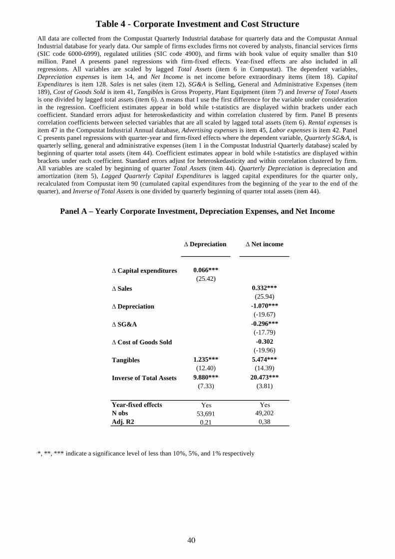
In order to verify that a discretionary reduction in investment creates earnings surprises through

the depreciation channel, I perform the same regressions as the one presented above, replacing

variable Capital expenditures with Depreciation. Depreciation is the ratio of depreciation and

amortization expenses (item 14 in Compustat) scaled by lagged total assets (item 6). The results are

presented in Table 6. The results remain identical to those discussed previously with respect to most

of the comparable coefficients. What is interesting is that the coefficient on Depreciation is

negative and significant at the 1% level in all specifications except the last one, where it is still

significant at the 5% level. A reduction in depreciation increases the probability to create positive

earnings surprises. As discussed in section 2, a reduction in investment will directly reduce

depreciation expenses. A reduction in expenses will increase earnings and contribute to increase the

likelihood that firms meet or beat analysts’ consensus EPS forecasts.

[Insert table 6 about here]

As discussed in section 3, simultaneity biases should not be too much of a concern, because the

two stories that are consistent with this bias and the effects that we find are at odds with the existing

empirical evidence. The story that investment decisions could be jointly determined by a shock that

also affects analysts’ prediction abilities in the same fiscal year is inconsistent with the evidence

found by Easterwood and Nutt (1999). These authors find that analysts underreact to bad news and

overreact to good news contained in prior year’s performance. Elliott, Philbrick and Weidman

24

(1995) find that analysts underreact to good and bad news during the fiscal year, contradicting the

story that bad news, associated with reduced investment, could be positively correlated with more

positive earnings surprises. This is further confirmed by results from regressions presented in Table

5 and 6. The coefficient on variable Upwards consensus change is positive and the coefficient on

Past Profitability is negative.

Alternatively, the story that investment decisions could be jointly determined by a shock that

also affects the firms’ earnings in the same fiscal year is also inconsistent with the finding that

analysts underreact to restructuring news (Chaney, Hogan and Jeter, 1999). However, to rule out

any concerns about the direction of the causality between investment and earnings surprises, I

exploit the Compustat Quarterly Industrial database to test models where earnings surprises are

regressed against investment in earlier periods. I include all the control variables from the previous

specification in these regressions. The results are reported in Table 7.

Column 1 reports the results for a regression where Above consensus EPS forecast, based on

the consensus for the current fiscal year, is regressed against Lagged Capital Expenditures, capital

expenditures from the previous fiscal year. Columns 2 to 5 report the results for a regression where

Above consensus EPS forecasts in 4th quarter, the consensus forecast for the 4th quarter EPS, is

regressed against Capital expenditures in the first semester in column 2, and in the first, second and

third quarters of the same fiscal year in column 3 to 5 respectively. Note that these variables are

including total investment for the period considered only. I do not rebase these investment variables

on a yearly rate basis. As a result, firms invest approximately half of what is invested in a year in

the first semester, while in a quarter, firms invest about one fourth of what is invested in a year.

The previously discussed results remain robust to these new specifications. Decreased

investment in earlier periods increases the probability that a firm will create positive earnings

surprises in the future. Therefore, one can confidently conclude that a reduction in investment at the

firm level will help create positive earnings surprises.

[Insert table 7 about here]

What is striking in the results presented in Table 7 is that analysts do not seem to fully grasp

the effects that investment will have on the earnings they forecast. These capital expenditures data

are available to them, so they should be able to infer that a reduction in investment will result in

higher earnings and adjust their forecasts accordingly. Even capital expenditures in the previous

fiscal year can positively predict earnings surprises in the next fiscal year.

However, note that this relationship was not so easy to disentangle at first sight, because the

simple univariate correlation between investment and earnings surprises was significantly positive.

25

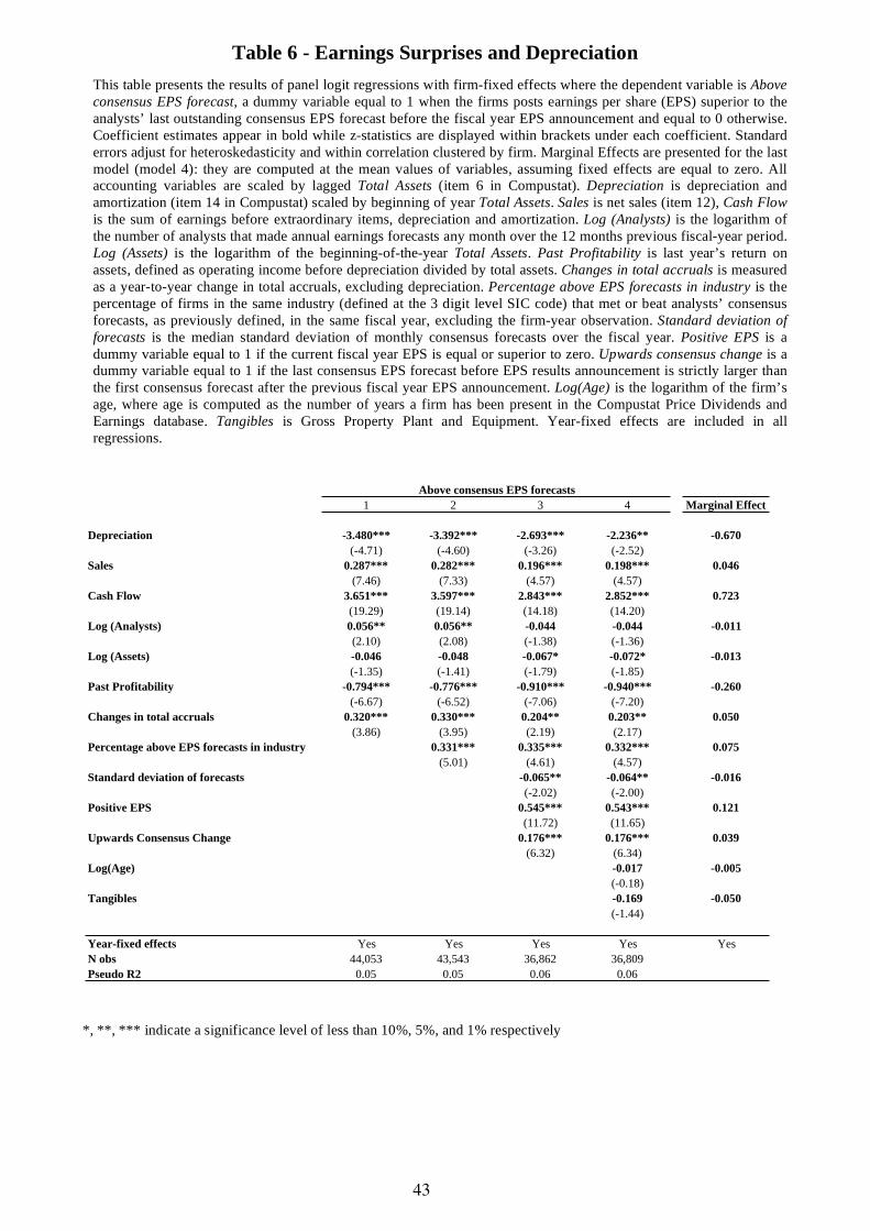
5.4 Analyst Pressure Hypothesis

I now move to the analysis of hypothesis H3. It states that firms facing abnormally high

pressure from analysts, in the form of abnormally high EPS consensus forecasts at the start of the

year, will invest less all else being equal. Table 8 reports the results from estimating equation (3) on

my sample of firms, using Capital expenditures as the dependent variable and variable Analyst

Pressure in all specifications. Column 1 estimates a simple model with lagged Tobin’s Q,

contemporaneous cash flow, a logarithm transformation of lagged analyst coverage, past return on

assets and the logarithm transformation of lagged total assets as controls. In the following columns,

I add various other control variables. Column 2 adds a control for financials constraints in the form

of the Kaplan and Zingales (1997) index and an interaction term between this control and lagged

Tobin’s Q. These variables control for the fact that financially constrained firms invest less than

unconstrained firms (Kaplan and Zingales, 1997). Furthermore, Baker, Stein and Wurgler, 2003

find that financially constrained firms have corporate investment policies that are sensitive to stock

price variations. They invest more when stock prices are high and less when stock prices are low.

Hence I introduce an interaction term between Tobin’s Q and the Kaplan and Zingales (1997)

index. Column 3 adds a proxy for firm age, and a proxy for value firms. Firms at early stages of

their development are expected to invest more than mature firms, while value firms may invest less

than growth firms. Finally, I add a control for stock price misvaluation in column 4. Indeed, as

found in Baker, Stein and Wurgler (2003), firms invest more when overvalued, i.e. when they have

low future excess stock returns.

Overall, the coefficient on Analyst pressure is negative and significant at the 1% level in all

specifications. It is estimated at -2.447 in column 1 and at -1.466 in column 3. Economically this

suggests that a firm facing abnormally high analyst forecasts increasing by a one (within-firm)

standard deviation decreases investment by 0.10% to 0.16% of total assets. This represents a

decrease of 2% to 3% of median corporate investment or a decrease of 1% to 2% of mean corporate

investment.

Coefficients on the control variables are consistent with previous results from the investment

literature. Firms invest more the better the investment opportunities, as proxied by Tobin’s Q.

Firms also invest more the larger the contemporaneous cash flow. Fazzari Hubbard and Petersen

(1988) claim that firms that face financial constraints will be sensitive to cash flow shocks and will

adjust the investment level to the level of available cash flow. Alti (2003) argues that cash flow

shocks contain information that is not properly captured by Tobin’s Q. Firms with positive cash

flow shocks should invest more, even in the absence of financial constraints. Consistent with

Doukas et al. (2006), firms invest more the more intense the analyst coverage, as analysts reduce

asymmetric information with the stock market. Firms also invest more the higher the past

26

profitability and less the larger their size, as measured by the logarithm of Assets. In addition firms

with large financial constraints invest less (Kaplan and Zingales, 1997), and are more sensitive to

stock price variations (Baker, Stein and Wurgler, 2003). Firms also invest less when they grow

older and the larger their total assets base. All firms, irrespective of their level of financial

constraints, invest more when they are overvalued (Baker, Stein and Wurgler, 2003).

[Insert table 8 about here]

5.5 Investment Postponement Hypothesis

So far, we have shown that firms investing less than usual in a year create more non-negative

earnings surprises, and that firms facing high analyst pressure reduce investment. I also posited, in

hypothesis H2, that the reduction in investment that is intended to cause the earnings surprise will

be temporary and lead to a subsequent increase in investment. If the firms’ reduction in investment

caused by beating EPS consensus forecasts is temporary, i.e. the firms compensate the reduction in

investment at time t-1 by investing more at time t, we should observe a positive correlation between

the lagged value of Above consensus EPS forecastit-1 and Capital expenditures. This is the result

that we get from estimating equation (4) as exhibited in Table 9. The coefficients of Above

consensus EPS forecastit-1 are positive and significant at the 1% level.

[Insert table 9 about here]

5.6 Robustness Checks

I perform several robustness checks relative to the previous choices of variables and

specifications.

First, I construct an alternative measure of analysts consensus forecast using the last forecast

reported by a sell-side analyst in the I/B/E/S Individual Detail files13 before the EPS reporting date.

This measure has been used in the earnings surprise literature as an alternative to the last median

EPS forecast in the I/B/E/S Individual Summary files on the grounds that it reflects more up to date

information by analysts issuing forecasts in the vicinity of the reporting date. The use of such

variable makes sense in those analyses, because researchers are primarily interested in earnings

management that is decided right before the reporting date, through e.g. accruals management. In

our case, however, using the baseline consensus forecasts makes more sense as the investment

decisions by managers should be influenced less by the desire to meet or beat the very last analyst

EPS forecast, that is unknown yet. Indeed the investment decisions have been made already, and for

the most part have been reported in previous quarterly reports. Managers have no way to influence

the meeting or the beating of such late forecast through a reduction in investment. However, I use

13 I again use the file with unadjusted data for stock splits, and adjust them using the procedure recommended by

WRDS in Robinson and Glushkov (2006).

27

this forecast variable to further strengthen the results that were found in previous regressions, and to

further argue that analysts do not seem to take into account the effect of investment reduction on

earnings surprises. The results of model (1) with this new variable as the dependent variable are

presented in Table 10. The coefficient on Capital expenditures is always negative in all

specification of the model with a significance level of 1% and 5% in column 3 and 4 respectively.

The significance is slightly reduced relative to the main specification, especially in specifications

where fewer controls are included (column 1 and 2). Nevertheless, this reduced significance was

expected, as discussed above. Analysts issuing forecasts before the reporting date should

incorporate more information about the effects corporate investment has on earnings. Still, they do

not incorporate enough information to cancel out the negative impact of investment on earnings

surprises.

[Insert table 10 about here]

Second, I build a measure of sales surprises to check that sales surprises are not correlated with

investment, because in my story, they have no reasons to be. A reduction in investment creates

surprises in costs (depreciation and collateral expenses) that are not fully accounted for by analysts.

Therefore, investment should not be significantly negatively correlated with sales surprises. I

construct variable Above analysts’ sales consensus forecast as a dummy variable equal to one if

actual sales are larger than the analysts’ sales consensus forecast and equal to zero otherwise. The

analysts’ sales consensus forecast is constructed in the exact same way as the EPS consensus

forecast used in the baseline analysis and described in section 4. I take the last median consensus

forecast from the I/B/E/S Summary files. Because sales forecast are scarcer in the I/B/E/S

database14, the number of observations available for our analysis drops from 65,221 for the period

1981 to 2005 to 17,895 firm-year observations for the period 1993 to 2005. In addition, because of

the specific procedures used in the fixed effects logit estimation and the various variable

requirements, the number of firm year-observations drops to numbers ranging from 10,562 to

11,793 firm-year observations, depending on the specification. The number of observations should

be large enough to obtain good estimation from the logit fixed-effects regressions.

As expected, results reported in Table 11 show that there is no significant negative correlation

between sales surprises and investment. The coefficient on Capital expenditures is negative in all

specifications, but is not significant at any usual level. The z statistics are low, ranging from 0.51 to

1.08. Sales surprises are not negatively correlated with investment. This result is consistent with

the analysts’ general prediction ability not being correlated with investment, whereas the analysts’

prediction ability concerning the firms’ costs is correlated with investment.

[Insert table 11 about here]

14 Data on sales forecasts and sales realizations have been collected from year 1993 onwards in I/B/E/S.

28

Taken together, the results of section 5 suggest that firms that invest less in a given year will

increase their probability to meet or outperform analysts’ EPS consensus forecasts in the same year.

This result is obtained through the creation of surprises in costs. We identified more specifically

surprises in depreciation expenses, but surprises in other collateral expenses could also explain this

result.

6 Increased Underinvestment or Reduced Overinvestment?

An interesting question is whether the reduction in investment induced by consensus fixation

corresponds to a reduction of overinvestment, or the passing up of valuable investment

opportunities.

Testing such question is difficult because the profitability of project investment is

unobservable. Moreover, it is not clear whether the average firm in the sample is (i) investing the

right amount of money, is (ii) underinvesting or (iii) overinvesting. Therefore, observing a

reduction in investment can be interpreted as underinvestment under hypothesis (i) or an

aggravation of the underinvestment problem under hypothesis (ii). Under these two assumptions,

the results presented thus far support the view that analysts create an adverse effect on investment

through increased underinvestment. Conversely, under hypothesis (iii), the observation of a

reduction in investment to create earnings surprises can be interpreted as an improvement in the

firms’ capital budgeting policy through reduced overinvestment.

Recent empirical evidence provided by Bertrand and Mullainathan (2003) and Bøhren, Cooper

and Richard (2007) suggests that overinvestment is not the norm among U.S. firms. Managers enjoy

the “quiet life”. They tend to underinvest rather than overinvest. Bøhren, Cooper and Richard

(2007) show that firms where managers are more entrenched tend to invest less than firms in which

governance mechanisms protect shareholders more against managerial discretion. Based on these

results, the reduction in investment found previously is difficult to reconcile with a beneficial effect

for firms and their shareholders. Nevertheless, to further strengthen this argument, I address the

issue using two different perspectives.

In the first approach, I rank firms based on their corporate governance quality. Consistent with

the arguments in Jensen (1986), I posit that firms in which agency costs are high are more

susceptible to overinvestment than firms in which agency costs are low. Self-serving managers may

want to build empires at the expense of shareholders. Managers may be given less leeway by the

shareholders and the board to pursue pet projects and unprofitable investment opportunities in firms

in which good corporate governance mechanisms are in place (Gompers, Ishii and Metrick, 2003).

Firms in which shareholders are less protected against managerial discretion are more susceptible to

overinvestment than firms with stringent shareholders’ rights protection. Therefore these firms are

29

expected to decrease more their investment to meet or beat consensus forecasts if the decrease in

investment associated with beating EPS consensus forecasts is beneficial (overinvestment is

reduced). On the other hand, observing a larger reduction to create earnings surprises among the

firms with better corporate governance could be interpreted as a proof of the increased short-term

pressure brought about by analysts’ consensus EPS forecasts. Firms in which managers are less

protected are more likely to be ousted by unhappy shareholders after bad firm performance

(Fisman, Khurana and Rhodes-Kropf (2004)). Therefore, it is in those firms that managers have the

highest incentives to keep the shareholders’ happy in the short term. Beating consensus forecasts is

one such way of keeping shareholders happy.

I test these two hypotheses by using two different measures of corporate governance. The first

measure is the Gompers, Ishii and Metrick (2003) index of corporate governance, and the second

measure is the Bebchuk, Cohen, and Ferrell (2004) managers’ entrenchment index. Gompers, Ishii

and Metrick (2003) construct their governance index by considering all provisions from a company

corporate charter reported by IRRC (Investors Responsibility Research Center) that go against the

protection of the firms’ shareholders. A total of 24 unique provisions are considered, and, for every

firm, the authors add one point for each provision that restricts shareholders’ rights. Thus Git has a

possible range from 1 to 24, where the lowest values of Git stand for the firms with the best

shareholders’ rights protections and the highest Git values stand for the firms with the worst such

protection provisions. Bebchuk, Cohen and Ferrell (2004) argue that only six such provisions need

be considered in the construction of a corporate governance index: staggered boards, limits to

shareholder bylaw amendments, supermajority requirements for mergers, supermajority

requirements for charter amendments, poison pills and golden parachutes. The first four provisions

prevent a majority of shareholders from having their way, while the last two provisions make a

hostile takeover more costly, and thus less likely. This index actually measures managers’

entrenchment.

I construct the portfolios of corporate governance as follows. I classify firms as belonging to a

governance tercile based on their previous year corporate governance index value. I then run

regressions where Capital expenditures is the control variable in the logit specification. I use

terciles because of the lower number of observations available for these indices. I only get the

Gompers, Ishii and Metrick (2003) governance index for 15,421 firm-year observations and the

Bebchuk, Cohen, and Ferrell (2004) managers’ entrenchment index for 13,856 firm-year

observations. The firms in that sample are biased towards large firms.

Results for the logit firm fixed effects specification are presented in Table 12 Panel A and

Panel B. Panel A shows the results for the portfolios constructed based on the Gompers, Ishii and

Metrick (2003) governance index. Panel B does the same for portfolios based on the Bebchuk,

30

Cohen, and Ferrell (2004) managers’ entrenchment index. Higher scores of these indices mean

worse corporate governance, so that the bad governance firms are ranked in the last tercile and good

governance firms are ranked in the first tercile.

The results in Table 12 Panel A and B seem to confirm the hypothesis that the previously

observed reduction in investment to create earnings surprise is not primarily present among weakest

governance firms. The regressions in the lowest tercile portfolios, firms with the best governance

mechanisms according to both indices, are the only portfolio in which the negative coefficients are

significant. The significance level is at the 1% level despite the low number of observations. This

result suggests that firms with less entrenched managers are more subject to a reduction in

investment to create positive earnings surprises than firms with more entrenched managers. One

could be tempted to interpret this finding as a proof of the analysts’ induced managerial short-term

bias. However the low number of observations in tercile 2 and 3 advocate for caution in the

interpretation of these findings15. Nevertheless, one can confidently discard the hypothesis that the

reduction in investment related to earnings surprise that we found previously is driven by weak

governance firms. In those conditions, it appears difficult to argue that such reduction in investment

is beneficial to firms in our sample.

Panel C and Panel D report the results for the estimation of model (3) where firms are ranked

by governance index. The reported results show that variable Analyst pressure is no longer

negatively correlated with Capital expenditures in any of the governance portfolio at a significant

level. Firms facing high pressure from analysts early in the year do not significantly reduce

investment more when firms have weak or strong corporate governance mechanisms. Again, the

results previously found in section 5.4 do not appear to be driven by weak corporate governance

firms.

[Insert table 12 about here]

In the second approach, I rank firms based on their investment opportunity set. If the reduction

in investment induced by consensus beating occurs because it purges excess investment, it should

be stronger for firms with low investment opportunities. Indeed these firms are those for which, for

a given level of investment, the percentage of investment that is excessive is higher. It turns out that

firms with good investment opportunities decrease more their investment to beat consensus than

firms with bad investment opportunities, as shown in Table 13 Panel A. Firms in the lowest Tobin’s

Q tercile, the firms that have the lowest investment opportunities, do not decrease their investment

to create earnings surprises. Although the coefficient on Capital expenditures is negative, it is not

significant at conventional levels. On the other hand, firms with the largest investment

15 The governance index variables are discrete with a limited range (from 1 to 24 for the Gompers, Ishii and Metrick

(2003) index and from 1 to 6 for the Bebchuk Cohen and Ferrel (2004) index) and are biased towards low values of the

index. This can explain the imbalance in the number of firm-year observations in the three terciles.

31

opportunities, firms in the highest Tobin’s Q tercile have a large negative coefficient on Capital

expenditures. It is significantly negative at the 1% level and more negative than the coefficient for

firms in the second tercile. The significance level is also larger. This, again, suggests that the

reduction in investment related to consensus beating is not beneficial to the firms in our sample.

Panel B also reports that firms with high Tobin’s Q, firms in the highest tercile, respond even

more than other firms by reducing investment as a response to analyst pressure. The interaction

term between variable High Tobin’s Q and Analyst pressure is negative and significant at the 10%

level.

[Insert table 13 about here]

These results suggests that we cannot attribute the previously found reduction in investment to

create positive earnings surprises to firms that are not aligned with their shareholders interests, or to

firms that do not have large investment opportunities. These results are consistent with firms giving

up or postponing profitable investment opportunities to create positive earnings surprises.

7 Conclusion

Analysts seem to exert adverse short-term pressure on the firms they follow when capital

budgeting decisions are concerned. This pressure is exerted through their earnings per share

forecasting activity. Firms invest less to outperform analysts’ consensus EPS forecasts and firms

reduce investment when analysts’ consensus EPS forecasts are abnormally high at the start of the

year. The reduction in investment related to earnings surprises and abnormal analyst pressure is not

beneficial to the weaker corporate governance firms or to the firms with lowest investment

opportunities. These findings suggest that analysts may play a role in the managers’ myopia as

suggested in Stein (1989). It is difficult to conclude whether the negative impact analysts have on

corporate investment outweigh the benefits of reduced information asymmetry previously identified

in the literature (Chen et al. (2006) and Doukas et al. (2006)). Financial analysts may indeed relieve

firms from these constraints on investment. However they also seem to encourage underinvestment

at the firm level in order to meet consensus EPS forecasts. This result suggests that, as found by

Graham, Harvy and Rajgopal (2005) in a survey of American CFOs, managers are ready to sacrifice

investment projects to meet their desired earnings targets.

References

Baker M., Stein J. and J. Wurgler, 2003. “When Does the Market Matter? Stock Prices and the Investment of Equity-Dependent Firms”, The Quarterly Journal of Economics, 118, 969-1006.

Bebchuk, L., A. Cohen and A. Ferrell, 2004. "What Matters in Corporate Governance?" Harvard

Law School John M. Olin Center Discussion Paper No. 491 Available at SSRN: http://ssrn.com/abstract=593423

32

Bertrand, M., and S. Mullainathan, 2003. “Enjoying the quiet life? Corporate governance and managerial preferences”, The Journal of Political Economics, 111, 1043-1075.

Bhushan, R., 1989. “Firm Characteristics and Analyst Following”, Journal of Accounting and

Economics, 11, 255-274. Bøhren, Ø., Cooper, I. and P. Richard, 2007. “Corporate Governance and Real Investment

Decisions”. Available at SSRN: http://ssrn.com/abstract=891060 Brown, L.D., 2001. “A Temporal Analysis of Earnings Surprises: Profits vs. Losses”, Journal of

Accounting Research, 39, 221-241.

Burgstahler, D., and M. Eames. 2006. “Management of Earnings and Analysts’ Forecasts”, Journal of Business Finance & Accounting, 33, 633–652.

Bushee, B., 1998. “The influence of Institutional Investors on Myopic R&D Investment Behavior”.

Accounting Review, 73, 305-333. Chaney, P., Hogan C. and D. Jeter, 1999. “The Effect of Reporting Restructuring Charges on

Analysts’ Forecast Revisions and Errors”. Journal of Accounting and Economics, 27, 261 -284.

Chang X., Dasgupta S. and G. Hilary, 2006. “Analyst Coverage and Financing Decisions”, Journal

of Finance, Forthcoming. Chen Q., Goldstein I. and W. Jiang, 2006. “Price Informativeness and Investment Sensitivity to

Stock Price”, Review of Financial Studies, Forthcoming. Das, S., Levine, C.B. and K Sivaramakrishnan, 1998. “Earnings predictability and bias in analysts’

earnings forecasts”, Accounting Review, 73, 277-294. De Angelo, L., 1986. “Accounting Numbers as Market Valuation Substitutes: a Study of

Management Buyouts of Public Stockholders”, Accounting Review, 61, 400-420. Dechow, P.M., Sloan, R.G and A.P Sweeney, 1995. “Detecting Earnings Management”. Accounting

Review, 70, 193-225. Degeorge, F., Ding, Y., Jeanjean, T. and R. Stolowy, 2005. “Can Analysts Curb Earnings

Management? International Evidence”. Working Paper Degeorge, F., Patel, J. and R. Zeckauser, 1999. “Earnings Management to Exceed Thresholds”.

Journal of Business, 72, 1-33. Degeorge, F., Patel, J. and R. Zeckauser, 2007. “Earnings Thresholds and Market Responses”.

Working Paper Diether, K.B., Malloy, C.J. and A. Scherbina, 2002, “Differences of Opinion and the Cross Section

of Stock Returns”, Journal of Finance, 57, 2113-2141. Doukas, J.A., Kim, C. and C. Pantzalis, 2006. “Do Analysts Influence Corporate Financing and

Investment”. European Financial Management, forthcoming.

33

Easterwood, J. C. and S. R. Nutt, 1999. “Inefficiency in Analysts’ Earnings Forecasts: Systematic Misreaction or Systematic Optimism?”, Journal of Finance, 54, 1777-1797.

Elliott, J.A., D.R. Philbrick and C.I. Weidman, 1995. “Evidence from Archival Data on the Relation

Between Security Analysts’ Forecast Errors and Prior Forecast Revisions”, Contemporary

Accounting Research, 11, 919-938. Fazzari, S.M., Hubbard, R.G. and B.C. Petersen, 1988. “Financing Constraints and Corporate

Investment”. Brookings Papers on Economic Activity, 141-195. Fisman, R., Khurana, R. and M. Rhodes-Kropf, 2004. “Governance and CEO Turnover: Do

Something or Do the Right Thing?”, Working Paper Gompers, P. A., Ishii, J. L. and A. Metrick, 2003. "Corporate Governance and Equity Prices", The

Quarterly Journal of Economics, 118(1), 107-155. Graham J., Harvey C. and S. Rajgopal, 2005. “The Economic Implications of Corporate Financial

Reporting”, Journal of Accounting and Economics, 40, 3-73 Hausman, J. A., 1978, “Specification tests in econometrics”, Econometrica, 46, 1251-1271. Jensen, M.C., 1986. “Agency Costs of Free Cash Flow, Corporate Finance and Takeovers”,

American Economic Review, 76, 323-329. Jensen, M.C., and J. Fuller, 2002. “Just Say No To Wall Street”, Journal of Applied Corporate

Finance, Vol. 14, No. 4, 41-46. Kaplan, S.N. and L. Zingales, 1997. “Do Investment-Cash Flow Sensitivities Provide useful

Measures of Financing Constraints?”, Quarterly Journal of Economics, 112, 159-216. Kinney, W., D. Burgstahler and R. Martin, 2002. “The Materiality of Earnings Surprises”, Journal

of Accounting Research, 40, 1297-1329. Li, K. and X. Zhao, 2006. “Analyst Coverage and Dividend Policy”, Working Paper, University of

British Columbia. Matsumoto, D.A., 2002. “Management’s Incentives to Avoid Negative Earnings Surprises”, The

Accounting Review, 77, 483-514. O’Brien, P.C., 1988. “Analysts Forecasts as Earnings Expectations”, Journal of Accounting and

Economics, 10, 53-83. Robinson, D. and D. Glushkov, 2006. “A Note on IBES Unadjusted Data”, Wharton Research Data

Services. Roychowdhury, S., 2006. “Earnings Management Through Real Activities Manipulation”, Journal

of Accounting and Economics, 42, 335-370. Skinner, D. and R. Sloan, 2002. “Earnings Surprises, Growth Expectations, and Stock Returns or

Don’t Let an Earning Torpedo Sink your Portfolio”, Review of Accounting Studies, 7, 289-312.

34

Stein, J., 1989. “Efficient Capital Markets, Inefficient Firms: a Model of Myopic Corporate Behavior”, Quarterly Journal of Economics, 104, 655-669.

Wooldridge, J.M., 2002. Econometric Analysis of Cross Section and Panel Data, MIT Press,

Cambridge, Massachussets. Yu, F., 2006. “Analyst Coverage and Earnings Management”, Working Paper, University of

Minnesota.

35

Table 1 - Construction of the Analyst Pressure Proxy

Variable Analyst Pressure is the residual of the following panel regression with firm-fixed effects. The dependent

variable is Forecast EPS change, the forecast change in EPS from last year’s realized EPS, normalized by lagged stock

price, (EPS forecaststart of year t - actual EPSt-1)/Stock price t-1-90days. Coefficient estimates appear in bold while t-statistics are

displayed within brackets under each coefficient. Standard errors adjust for heteroskedasticity and within correlation

clustered by firm. Tobin’s Q is the beginning of the year market-to-book ratio computed as the market value of equity

plus book value of assets minus the book value of equity minus balance sheet deferred taxes scaled by the value of book

assets. Past Profitability is last year’s return on assets, defined as operating income before depreciation divided by total assets. Cash Flow (t-1) is the sum of earnings before extraordinary items, depreciation and amortization scaled by start-

of-year Total Assets (multiplied by 100) in the previous year. Positive EPS (t-1) is a dummy variable equal to 1 if last

fiscal year’s EPS is equal or superior to zero. Kaplan and Zingales (1997) index is a modified Kaplan and Zingales

(1997) index of Financial Constraints, excluding Tobin’s Q. Log (Analysts) is the logarithm of the number of analysts that

made annual earnings forecasts any month over the 12 months previous fiscal-year period. Forecast EPS change in

industry, is the average Forecast EPS change in the same industry (defined at the 3 digit SIC code level). Log (Assets) is

the logarithm of the beginning-of-the-year Total Assets. Expected positive turnaround is a dummy variable equal to 1 if

the forecast EPS for fiscal year t is positive and the actual EPS in year t-1 was negative. Expected negative turnaround is

a dummy variable equal to 1 if the forecast EPS for fiscal year t is negative and the actual EPS in year t-1 was positive.

Above consensus EPS forecast (t-1) is a dummy variable equal to 1 if the firm posted earnings per share (EPS) superior to

the analysts’ the last outstanding consensus EPS forecast before EPS announcement in the last fiscal year and equal to 0 otherwise. Year-fixed effects are also included.

*, **, *** indicate a significance level of less than 10%, 5%, and 1% respectively

Forecast EPS change

Tobin's Q -0.002***

(-3.64)

Past Profitability 0.029***

(2.59)

Positive EPS (t-1) -0.068***

(-13.59)

Cash Flow (t-1) -0.001***

(-8.04)

Kaplan and Zingales (1997) index 0.000***

(12.58)

Log (Analysts) -0.005***

(-3.88)

Forecast EPS change in industry 0.106***

(6.47)

Log (Assets) -0.009***

(-6.49)

Expected positive turnaround 0.039***

(7.91)

Expected negative turnaround -0.064***

(-14.27)

Above consensus EPS forecasts (t-1) -0.010***

(-11.71)

Year-fixed effects Yes

N obs 37,805

Adj. R2 0.51

36

Table 2 – Definition of Main Variables

Capital expenditures Capital expenditure (Compustat item 128) scaled by start-of-year total assets (item 6)

Total assets Start-of-year total assets (item 6) (in million USD)

Tobin’s Q Market value of equity (item 199 multiplied by item 25) plus book value of assets minus book value of equity minus deferred taxes (item 6 -

item 60 - item 74), scaled by book value of total assets (item 6). Variable is lagged one year

Past profitability Ratio of operating income before depreciation and amortization (item 13) to start-of-year total assets. Variable is lagged one year

Cash flow Net income before extraordinary items (item 18) + depreciation and amortization expenses (item 14) scaled by start-of-year total assets

Kaplan and Zingales (1997)

index

Start-of-year Kaplan-Zingales (1997) index of equity dependence (excluding Tobin’s Q): Kaplan and Zingales index (1997) index = -1.002*Cash Flow -39.368*Dividends -1.315*Cash +3.139*Leverage

Dividends is Common stock dividends (item 21) + Preferred Stock dividends (item 19) scaled by start-of-year total assets. Cash is item 1

scaled by start-of-year assets Leverage is long-term debt (item 9) plus debt in current liabilities (item 34) divided by total debt (item 9 + item

34) plus book value of common equity (item 216)

Firm age Number of years the company has been present in the Compustat Price Dividend and Earnings database

Positive EPS Dummy variable equal to 1 if the current fiscal year EPS (earnings per share) is equal or superior to zero

Analysts Maximum number of analysts that posted EPS forecasts any month during the fiscal year for the fiscal year-end. Variable is lagged one year

Above EPS consensus

forecasts

Dummy variable equal to 1 when EPS is above the last analysts’ consensus forecast published before EPS reporting date

Percentage above EPS

forecasts in industry

Percentage of firms in the same industry (at 3 digit SIC code level) that posted EPS above last EPS analysts consensus forecasts

Analyst pressure Proxy for the level of analyst pressure at the beginning of the fiscal year. The variable is constructed as the residual of a firm- and year- fixed

effects panel regression where the forecast increase in EPS from last year’s realized EPS, normalized by lagged stock price, (EPS forecaststart

of year t - actual EPSt-1)/Stock price t-1-90days, is regressed against Past profitability, lagged Above EPS consensus forecasts, Tobin’s Q, lagged

Cash flow, Kaplan and Zingales (1997) index, lagged Positive EPS, lagged log(Analysts), lagged log(Total Assets), and other specific

variables (see section 4 page 12 and 13 of main text and table 1 for details)

Upwards forecast revisions Dummy variable equal to 1 if the latest EPS consensus forecast before EPS announcement is larger than the first EPS consensus forecast

Changes in total accruals Changes in total accruals from year t-1 to year t. Total accruals are defined as changes in current assets (item 4) minus changes in cash (item

1) minus changes in current liabilities (item 5) plus changes in current maturities of long term debt (item 44) plus changes in income taxes

payable (item 71), all of these variables being scaled by beginning of the year total assets

Baker Stein and Wurgler’s

(2003) undervaluation

Compounded cumulative excess return (stock market return for the firm minus the value weighted stock market return) computed from CRSP

over fiscal year t+1 to year t+3, as in Baker, Stein and Wurgler (2003)

37

Table 3 – Summary Statistics Data are collected from the merged CRSP/Compustat Industrial database and I/B/E/S for the years 1981 to 2005 and exclude firms not covered by analysts, financial services firms (SIC

code 6000-6999), regulated utilities (SIC code 4900), and firms with book value of equity smaller than $10 million. Capital Expenditures is Compustat item 128 scaled by start-of-year

Total Assets. Total Assets is the beginning-of-the-year total assets. Tobin’s Q is the lagged market-to-book ratio. Past profitability is the lagged return on assets computed as income before

extraordinary items scaled by Total Assets. Kaplan and Zingales (1997) index is a modified Kaplan and Zingales (1997) index of Financial Constraints, excluding Tobin’s Q, Cash Flow is

the sum of earnings before extraordinary items, depreciation and amortization scaled by start-of-year Total Assets. Firm Age is the number of years a company has been present in the

Compustat Price Dividend and Earnings database. Analysts is the number of analysts that make annual earnings forecasts over the 12 months previous fiscal-year period. Above EPS

consensus forecasts is a dummy variable equal to 1 when the firm posts earnings per share (EPS) superior to the last analysts’ consensus EPS forecast and equal to 0 otherwise.

Percentage above EPS forecasts in industry is the percentage of firms in the same industry (defined at the 3 digit level SIC code) that met or beat analysts consensus forecasts in the same

fiscal year, as previously defined, excluding the firm-year observation. Analyst pressure is a proxy for the level of analyst pressure at the beginning of the fiscal year. The variable is constructed as the residual of a firm-fixed effects panel regression where the consensus forecast change in EPS from last year’s realized EPS, normalized by lagged stock price, is

regressed against a set of lagged variables controlling for past firm performance, firms characteristics and analyst coverage. Upwards forecast revisions is a dummy variable equal to 1 if

the latest EPS consensus forecast before EPS announcement is strictly larger than the first EPS consensus forecast. Changes in total accruals is measured as a year-to-year change in total

accruals. Baker, Stein and Wurgler (2003)’s undervaluation is the compounded cumulative excess return (stock market return for the firm minus the value weighted stock market return)

computed from CRSP over fiscal year t+1 to year t+3, as in Baker, Stein and Wurgler (2003). All data, except Firm Age, Analysts and the dummy variables, are winsorized at the 1st and

99th percentile. Panel A reports summary statistics, the number of observations (N), the mean, median and standard deviation of the key variables in our analysis for the overall sample of

firms covered by analysts, and for sub-samples of firms that met or beat analysts forecasts (Above EPS forecasts=1) and firms that did not (Above EPS forecasts=0). All variables scaled

by Total Assets are multiplied by 100. Panel B reports correlation among selected variables.

Panel A: Summary Statistics

*, **, *** indicate a significance level of less than 10%, 5%, and 1% respectively

Group mean

comparison test

N Mean Median Std. Dev. N Mean Median Std. Dev. N Mean Median Std. Dev.

H0: Difference is not

equal to 0

Capital expenditures 64,362 8.62 5.67 9.51 35,776 8.69 5.89 9.24 27,191 8.55 5.44 9.76 **

Total assets 65,221 1,415 181 4,963 36,192 1,663 233 5,421 27,599 1,144 137 4,39 ***

Tobin’s Q 62,597 2.09 1.48 1.91 34,533 2.17 1.55 1.95 26,67 1.99 1.39 1.85 ***

Past Profitability 54,931 12.78 15.00 20.64 30,738 14.83 16.47 19.44 23,36 10.55 13.32 21.46 ***

Kaplan and Zingales (1997) index 54,673 20.97 20.17 131.26 30,584 10.74 9.09 127.16 23,36 32.18 32.18 134.52 ***

Cash flow 64,998 5.41 9.46 21.25 36,06 9.11 11.47 18.31 27,52 1.25 6.76 22.95 ***

Firm age 65,221 14.53 11 10.60 36,192 15.11 12 10.91 27,599 13.92 11 10.23 ***

Analysts 62,750 7.59 5 7.50 35,917 8.46 6 7.73 26,599 6.46 4 7.02 ***

Above EPS consensus forecasts 63,791 0.57 1 0.50 36,192 1 1 0 27,599 0 0 0

Percentage above EPS forecasts in industry 63,122 0.57 0.58 0.18 35,797 0.58 0.60 0.18 27,325 0.54 0.55 0.18 ***

Analyst Pressure 37,805 0 0 0.07 21,939 -5E-4 -3E-4 0.06 15,729 6E-4 -7E-4 0.07

Upwards forecast revisions 62,750 0.44 0 0.50 35,917 0.44 0 0.50 26,599 0.44 0 0.50

Changes in total accruals 54,865 -0.86 -0.34 14.18 30,179 0.00 0.10 12.92 23,543 -1.96 -0.99 15.30 ***

Baker, Stein and Wurgler (2003)’s undervaluation 38,823 0.13 -0.17 1.26 23,187 0.13 -0.15 1.20 15,313 0.13 -0.20 1.32

Overall Sample

Sample of firms meeting or beating

analysts consensus forecast

Sample of firms NOT meeting or

beating analysts consensus forecast

38

Panel B: Correlation Among Key Variables

Capital

expenditures Total

assets Tobin’s

Q Past profi-

-tability

Kaplan

and

Zingales

(1997)

index Cash flow Firm

Age Analysts

Above

EPS

consensus

forecasts

Percentage

above EPS

forecasts

in industry Analyst

pressure

Upwards

forecast

revisions

Changes

in total

accruals

Capital expenditures 1

Total assets -0.03*** 1

Tobin’s Q 0.12*** -0.06*** 1

Past profitability 0.22*** 0.05*** -0.08*** 1

Kaplan and Zingales

(1997) index -0.02*** 0.03*** -0.30*** -0.14*** 1

Cash flow 0.17*** 0.06*** -0.19*** 0.71*** -0.13*** 1

Firm Age -0.13*** 0.29*** -0.20*** 0.13*** -0.02*** 0.17*** 1

Analysts 0.08*** 0.51*** 0.06*** 0.21*** -0.12*** 0.18*** 0.29*** 1

Above EPS consensus

forecasts 0.01* 0.05*** 0.05*** 0.10*** -0.08*** 0.19*** 0.05*** 0.13*** 1

Percentage above EPS

forecasts in industry -0.05*** 0.00 0.03*** -0.03*** -0.03*** -0.01 0.03*** -0.00 0.11*** 1

Analyst pressure -0.02*** 0.01 0.00 0.00 0.00 0.03*** 0.00 -0.01 -0.01* 0.01 1

Upwards forecast

revisions -0.01*** -0.00 0.06*** -0.11*** 0.07*** -0.10*** -0.06*** -0.01** -0.00 0.03*** -0.02*** 1

Changes in total

accruals 0.03** 0.01** -0.01* -0.09*** 0.00 0.12*** 0.04*** 0.01** 0.07*** 0.02*** 0.05*** 0.00 1

Baker, Stein and

Wurgler (2003)’s

Undervaluation -0.06*** -0.02*** -0.03*** -0.04*** 0.05*** -0.05*** -0.04** -0.04*** 0.00 0.00 -0.01 0.02*** -0.02***

*, **, *** indicate a significance level of less than 10%, 5%, and 1% respectively

39

Figure 1

Meeting or Not Analysts’ EPS Consensus Forecasts:

Ex-Ante Investment Opportunities and Investment Policy Evolution

Panel A displays the median firms’ ex-ante investment opportunities (Tobin’s Q) evolution over time for the sub-sample of firms that met or beat analysts consensus forecast at time t and

the sub-sample of firms that did not, while Panel B displays the median firms’ Capital Expenditures for the same two sub-samples. Tobin’s Q is the lagged market-to-book ratio computed

as the market value of equity plus book value of assets minus the book value of equity minus balance sheet deferred taxes scaled by the value of book assets, all values being measured at

the beginning of the fiscal year. Capital Expenditures is (Compustat) item 128 scaled by start-of-year Total Assets multiplied by 100.

Panel A – Median Lagged Tobin’s Q

Panel B – Median Capital Expenditures

40

Table 4 - Corporate Investment and Cost Structure

All data are collected from the Compustat Quarterly Industrial database for quarterly data and the Compustat Annual

Industrial database for yearly data. Our sample of firms excludes firms not covered by analysts, financial services firms

(SIC code 6000-6999), regulated utilities (SIC code 4900), and firms with book value of equity smaller than $10

million. Panel A presents panel regressions with firm-fixed effects. Year-fixed effects are also included in all

regressions. All variables are scaled by lagged Total Assets (item 6 in Compustat). The dependent variables,

Depreciation expenses is item 14, and Net Income is net income before extraordinary items (item 18). Capital

Expenditures is item 128. Sales is net sales (item 12), SG&A is Selling, General and Administrative Expenses (item

189), Cost of Goods Sold is item 41, Tangibles is Gross Property, Plant Equipment (item 7) and Inverse of Total Assets

is one divided by lagged total assets (item 6). means that I use the first difference for the variable under consideration

in the regression. Coefficient estimates appear in bold while t-statistics are displayed within brackets under each

coefficient. Standard errors adjust for heteroskedasticity and within correlation clustered by firm. Panel B presents

correlation coefficients between selected variables that are all scaled by lagged total assets (item 6). Rental expenses is

item 47 in the Compustat Industrial Annual database, Advertising expenses is item 45, Labor expenses is item 42. Panel

C presents panel regressions with quarter-year and firm-fixed effects where the dependent variable, Quarterly SG&A, is

quarterly selling, general and administrative expenses (item 1 in the Compustat Industrial Quarterly database) scaled by

beginning of quarter total assets (item 44). Coefficient estimates appear in bold while t-statistics are displayed within

brackets under each coefficient. Standard errors adjust for heteroskedasticity and within correlation clustered by firm. All variables are scaled by beginning of quarter Total Assets (item 44). Quarterly Depreciation is depreciation and

amortization (item 5), Lagged Quarterly Capital Expenditures is lagged capital expenditures for the quarter only,

recalculated from Compustat item 90 (cumulated capital expenditures from the beginning of the year to the end of the

quarter), and Inverse of Total Assets is one divided by quarterly beginning of quarter total assets (item 44).

Panel A – Yearly Corporate Investment, Depreciation Expenses, and Net Income

*, **, *** indicate a significance level of less than 10%, 5%, and 1% respectively

Depreciation Net income

Capital expenditures 0.066***

(25.42)

Sales 0.332***

(25.94)

Depreciation -1.070***

(-19.67)

SG&A -0.296***

(-17.79)

Cost of Goods Sold -0.302

(-19.96)

Tangibles 1.235*** 5.474***

(12.40) (14.39)

Inverse of Total Assets 9.880*** 20.473***

(7.33) (3.81)

Year-fixed effects Yes YesN obs 53,691 49,202

Adj. R2 0.21 0,38

41

Panel B – Correlation Between Yearly Investment, Depreciation,

Rental, Advertising and Labor expenses.

Capital expenditures

Lagged Capital

expenditures SG&A

expenses Depreciation

expenses Rental

expenses Advertising

expenses Labor

expenses

Capital

expenditures 1.00

Lagged Capital

expenditures 0.68*** 1.00

SG&A expenses -0.02*** -0.10*** 1.00

Depreciation

expenses 0.47*** 0.43*** 0.06*** 1.00

Rental expenses 0.17*** 0.13*** 0.38*** 0.19*** 1.00

Advertising

expenses 0.06*** 0.00 0.45*** 0.01** 0.15*** 1.00

Labor expenses 0.06*** 0.02 0.21*** 0.08*** 0.21** 0.04*

Number of total

observations 64,362 54,373 58,933 64,838 57,678 22,844 5,753

*, **, *** indicate a significance level of less than 10%, 5%, and 1% respectively

Panel C – Quarterly Corporate Investment and SG&A expenses

*, **, *** indicate a significance level of less than 10%, 5%, and 1% respectively

Quarterly SG&A

Quarterly depreciation 1.33***

(24.24)

Lagged quarterly capital expenditures 0.07***

(8.77)

Inverse of total assets 0.30***

(6.83)

Quarter-year-fixed effects YesN obs 165,746

Adj. R2 0.86

42

Table 5 - Earnings Surprises and Corporate Investment

This table presents the results of panel logit regressions with firm-fixed effects where the dependent variable is Above

consensus EPS forecast, a dummy variable equal to 1 when the firm posts earnings per share (EPS) superior to the

analysts’ last outstanding consensus EPS forecast before the fiscal year EPS announcement and equal to 0 otherwise.

Coefficient estimates appear in bold while z-statistics are displayed within brackets under each coefficient. Standard

errors adjust for heteroskedasticity and within correlation clustered by firm. Marginal Effects are presented for the last

model (model 4): they are computed at the mean values of variables, assuming fixed effects are equal to zero. All accounting variables are scaled by lagged Total Assets (item 6 in Compustat). Capital Expenditures is a fraction of

beginning of year Total Assets. Sales is net sales (item 12), Cash Flow is the sum of earnings before extraordinary

items, depreciation and amortization. Log (Analysts) is the logarithm of the number of analysts that made annual

earnings forecasts any month over the 12 months previous fiscal-year period. Log (Assets) is the logarithm of the

beginning-of-the-year Total Assets. Past Profitability is last year’s return on assets, defined as operating income before

depreciation divided by total assets. Changes in total accruals is measured as a year-to-year change in total accruals,

excluding depreciation. Percentage above EPS forecasts in industry is the percentage of firms in the same industry

(defined at the 3 digit level SIC code) that met or beat analysts’ consensus forecasts, as previously defined, in the same

fiscal year, excluding the firm-year observation. Standard deviation of forecasts is the median standard deviation of

monthly consensus forecasts over the fiscal year. Positive EPS is a dummy variable equal to 1 if the current fiscal year

EPS is equal or superior to zero. Upwards consensus change is a dummy variable equal to 1 if the last consensus EPS forecast before EPS results announcement is strictly larger than the first consensus forecast after the previous fiscal year

EPS announcement. Log(Age) is the logarithm of the firm’s age, where age is computed as the number of years a firm

has been present in the Compustat Price Dividends and Earnings database. Tangibles is Gross Property Plant and

Equipment. Year-fixed effects are included in all regressions.

*, **, *** indicate a significance level of less than 10%, 5%, and 1% respectively

1 2 3 4 Marginal Effect

Capital expenditures -0.575*** -0.617*** -0.740*** -0.775*** -0.178

(-2.73) (-2.92) (-3.19) (-3.33)

Sales 0.262*** 0.260*** 0.189*** 0.202*** 0.046

(6.88) (6.81) (4.49) (4.71)

Cash Flow 3.699*** 3.644*** 2.881*** 2.893*** 0.666

(19.37) (19.20) (14.16) (14.10)

Log (Analysts) 0.057** 0.057** -0.043 -0.040 -0.009

(2.08) (2.08) (-1.31) (-1.21)

Log (Assets) -0.040 -0.043 -0.067* -0.082** -0.015

(-1.16) (-1.26) (-1.76) (-2.08)

Past Profitability -0.727*** -0.706*** -0.848*** -0.895*** -0.206

(-6.14) (-5.96) (-6.58) (-6.85)

Changes in total accruals 0.305*** 0.315*** 0.183* 0.186** 0.043

(3.66) (3.76) (1.96) (1.99)

Percentage above EPS forecasts in industry 0.342*** 0.337*** 0.335*** 0.077

(5.12) (4.60) (4.56)

Standard deviation of forecasts -0.068** -0.065** -0.017

(-2.05) (-2.00)

Positive EPS 0.559*** 0.553*** 0.130

(12.00) (11.80)

Upwards Consensus Change 0.173*** 0.173*** 0.040

(6.18) (6.18)

Log(Age) -0.014 -0.003

(-0.16)

Tangibles -0.309*** -0.071

(-2.78)

Year-fixed effects Yes Yes Yes Yes Yes

N obs 43,539 43,030 36,405 36,356

Pseudo R2 0.05 0.05 0.06 0.06

Above consensus EPS forecasts

43

Table 6 - Earnings Surprises and Depreciation

This table presents the results of panel logit regressions with firm-fixed effects where the dependent variable is Above

consensus EPS forecast, a dummy variable equal to 1 when the firms posts earnings per share (EPS) superior to the

analysts’ last outstanding consensus EPS forecast before the fiscal year EPS announcement and equal to 0 otherwise.

Coefficient estimates appear in bold while z-statistics are displayed within brackets under each coefficient. Standard

errors adjust for heteroskedasticity and within correlation clustered by firm. Marginal Effects are presented for the last

model (model 4): they are computed at the mean values of variables, assuming fixed effects are equal to zero. All accounting variables are scaled by lagged Total Assets (item 6 in Compustat). Depreciation is depreciation and

amortization (item 14 in Compustat) scaled by beginning of year Total Assets. Sales is net sales (item 12), Cash Flow

is the sum of earnings before extraordinary items, depreciation and amortization. Log (Analysts) is the logarithm of

the number of analysts that made annual earnings forecasts any month over the 12 months previous fiscal-year period.

Log (Assets) is the logarithm of the beginning-of-the-year Total Assets. Past Profitability is last year’s return on

assets, defined as operating income before depreciation divided by total assets. Changes in total accruals is measured

as a year-to-year change in total accruals, excluding depreciation. Percentage above EPS forecasts in industry is the

percentage of firms in the same industry (defined at the 3 digit level SIC code) that met or beat analysts’ consensus

forecasts, as previously defined, in the same fiscal year, excluding the firm-year observation. Standard deviation of

forecasts is the median standard deviation of monthly consensus forecasts over the fiscal year. Positive EPS is a

dummy variable equal to 1 if the current fiscal year EPS is equal or superior to zero. Upwards consensus change is a dummy variable equal to 1 if the last consensus EPS forecast before EPS results announcement is strictly larger than

the first consensus forecast after the previous fiscal year EPS announcement. Log(Age) is the logarithm of the firm’s

age, where age is computed as the number of years a firm has been present in the Compustat Price Dividends and

Earnings database. Tangibles is Gross Property Plant and Equipment. Year-fixed effects are included in all

regressions.

*, **, *** indicate a significance level of less than 10%, 5%, and 1% respectively

1 2 3 4 Marginal Effect

Depreciation -3.480*** -3.392*** -2.693*** -2.236** -0.670

(-4.71) (-4.60) (-3.26) (-2.52)

Sales 0.287*** 0.282*** 0.196*** 0.198*** 0.046

(7.46) (7.33) (4.57) (4.57)

Cash Flow 3.651*** 3.597*** 2.843*** 2.852*** 0.723

(19.29) (19.14) (14.18) (14.20)

Log (Analysts) 0.056** 0.056** -0.044 -0.044 -0.011

(2.10) (2.08) (-1.38) (-1.36)

Log (Assets) -0.046 -0.048 -0.067* -0.072* -0.013

(-1.35) (-1.41) (-1.79) (-1.85)

Past Profitability -0.794*** -0.776*** -0.910*** -0.940*** -0.260

(-6.67) (-6.52) (-7.06) (-7.20)

Changes in total accruals 0.320*** 0.330*** 0.204** 0.203** 0.050

(3.86) (3.95) (2.19) (2.17)

Percentage above EPS forecasts in industry 0.331*** 0.335*** 0.332*** 0.075

(5.01) (4.61) (4.57)

Standard deviation of forecasts -0.065** -0.064** -0.016

(-2.02) (-2.00)

Positive EPS 0.545*** 0.543*** 0.121

(11.72) (11.65)

Upwards Consensus Change 0.176*** 0.176*** 0.039

(6.32) (6.34)

Log(Age) -0.017 -0.005

(-0.18)

Tangibles -0.169 -0.050

(-1.44)

Year-fixed effects Yes Yes Yes Yes Yes

N obs 44,053 43,543 36,862 36,809

Pseudo R2 0.05 0.05 0.06 0.06

Above consensus EPS forecasts

44

Table 7 - Controlling for Reversed Causality

This table presents the results of panel logit regressions with firm-fixed effects where the dependent variable are Above

consensus EPS forecast and Above consensus EPS forecast in the 4th

quarter, a dummy variable equal to 1 when the

firms posts earnings per share (EPS) superior to the analysts’ last outstanding consensus EPS forecast before the fiscal

year or fourth quarter EPS announcement and equal to 0 otherwise. Coefficient estimates appear in bold while z-

statistics are displayed within brackets under each coefficient. Standard errors adjust for heteroskedasticity and within

correlation clustered by firm. All accounting variables are scaled by lagged Total Assets (item 6 in Compustat). Capital

Expenditures is a fraction of beginning of year Total Assets. It is computed for the previous year, first semester, the 1st ,

2nd and 3rd quarters of the contemporaneous year from the Compustat quarterly Industrial database. All other financial

variables are yearly data. Sales is net sales (item 12), Cash Flow is the sum of earnings before extraordinary items,

depreciation and amortization. Log (Analysts) is the logarithm of the number of analysts that made annual earnings

forecasts any month over the 12 months previous fiscal-year period. Log (Assets) is the logarithm of the beginning-of-

the-year Total Assets. Past Profitability is last year’s return on assets, defined as operating income before depreciation

divided by total assets. Changes in total accruals is measured as a year-to-year change in total accruals, excluding

depreciation. Percentage above EPS forecasts in industry is the percentage of firms in the same industry (defined at the

3 digit level SIC code) that met or beat analysts’ consensus forecasts, as previously defined, in the same quarter,

excluding the firm-year observation. Standard deviation of forecasts is the median standard deviation of monthly

consensus forecasts over the fiscal year. Positive EPS is a dummy variable equal to 1 if the current fiscal year EPS is equal or superior to zero. Upwards consensus change is a dummy variable equal to 1 if the last consensus EPS forecast

before EPS results announcement is strictly larger than the first consensus forecast after the previous fiscal year EPS

announcement. Log(Age) is the logarithm of the firm’s age, where age is computed as the number of years a firm has

been present in the Compustat Price Dividends and Earnings database. Tangibles is Gross Property Plant and

Equipment. Year-fixed effects are included in all regressions.

*, **, *** indicate a significance level of less than 10%, 5%, and 1% respectively

Above consensus EPS forecasts

1 2 3 4 5

Lagged Capital Expenditures -0.464**

(-2.40)

Capital Expenditures 1st semester -2.126***

(-4.10)

Capital Expenditures 1st quarter -2.394**

(-2.38)

Capital Expenditures 2nd quarter -4.004***

(-4.55)

Capital Expenditures 3rd quarter -2.859***

(-3.64)

Sales 0.177*** 0.169*** 0.161*** 0.172*** 0.173***

(4.18) (3.74) (3.61) (3.79) (3.87)

Cash Flow 2.829*** 2.615*** 2.554*** 2.620*** 2.634***

(14.18) (13.37) (13.15) (13.36) (13.35)

Log (Analysts) -0.044 -0.012 -0.020 -0.013 -0.012

(-1.36) (-0.34) (-0.58) (-0.37) (-0.35)

Standard deviation of forecasts -0.063** -0.042 -0.043 -0.042 -0.042

(-1.98) (-1.48) (-1.51) (-1.50) (-1.49)

Percentage above EPS forecasts in industry 0.326*** 1.604*** 1.605*** 1.605*** 1.604***

(4.44) (21.02) (21.09) (21.03) (20.97)

Past Profitability -0.851*** -1.101*** -1.121*** -1.109*** -1.137***

(-6.42) (-7.82) (-7.96) (-7.90) (-8.11)

Changes in total accruals 0.196** 0.176* 0.163 0.172 0.164

(2.09) (1.67) (1.56) (1.64) (1.57)

Positive EPS 0.547*** 0.662*** 0.666*** 0.664*** 0.663***

(11.71) (13.22) (13.37) (13.25) (13.21)

Upwards Consensus Change 0.174*** 0.316*** 0.317*** 0.317*** 0.314***

(6.21) (10.39) (10.43) (10.42) (10.35)

Log(Age) -0.032 -0.033 -0.036 -0.031 -0.020

(-0.35) (-0.34) (-0.38) (-0.32) (-0.21)

Tangibles -0.291*** -0.205* -0.197 -0.207* -0.213*

(-2.61) (-1.65) (-1.60) (-1.67) (-1.72)

Log (Assets) -0.066* -0.082* -0.071* -0.082* -0.075*

(-1.69) (-1.91) (-1.66) (-1.91) (-1.76)

Year-fixed effects Yes Yes Yes Yes YesN obs 36,329 31,870 31,983 31,870 31,904

Pseudo R2 0.06 0.08 0.08 0.08 0.08

Above consensus EPS forecasts in 4th quarter

45

Table 8 - Corporate Investment and Measures of

Analyst Pressure on Management

This table presents the results of panel regressions with firm-fixed effects where the dependent variable is Capital

Expenditures (Compustat item 128), a fraction of beginning of year Total Assets (item 6) multiplied by 100. Coefficient

estimates appear in bold while t-statistics are displayed within brackets under each coefficient. Standard errors adjust

for heteroskedasticity and within correlation clustered by firm. Analyst Pressure is a proxy for the level of pressure

exerted by analyst at the start of the year on the firm’s management to increase earnings per share (EPS) relative to last

year’s EPS. Tobin’s Q is the beginning of the year market-to-book ratio computed as the market value of equity plus

book value of assets minus the book value of equity minus balance sheet deferred taxes scaled by the value of book

assets. Cash Flow is the sum of earnings before extraordinary items, depreciation and amortization scaled by start-of-

year Total Assets (multiplied by 100). Log (Analysts) is the logarithm of the maximum number of analysts that made

annual earnings forecasts any month over the 12 months previous fiscal-year period. Kaplan and Zingales (1997) index

is a modified Kaplan and Zingales (1997) index of Financial Constraints, excluding Tobin’s Q. Firm Age is the number

of years a company has been present in the Compustat Price Dividends and Earnings database. Tangibles is Gross

Property Plant and Equipment. Baker, Stein and Wurgler (2003)’s undervaluation is the cumulative excess return computed from CRSP over year t+1 to year t+3 as in Baker, Stein and Wurgler (2003). Year-fixed effects are included

in all regressions.

*, **, *** indicate a significance level of less than 10%, 5%, and 1% respectively

1 2 3 4

Analyst pressure -2.447*** -1.723*** -1.466*** -1.776***

(-5.44) (-3.88) (-3.31) (-2.62)

Tobin's Q 0.807*** 0.950*** 0.932*** 0.991***

(17.66) (18.07) (17.88) (13.33)

Cash Flow 0.035*** 0.035*** 0.036*** 0.043***

(7.15) (7.16) (7.36) (5.29)

Log (Analysts) 0.769*** 0.562*** 0.612*** 0.564***

(7.24) (5.32) (5.75) (3.69)

Past Profitability 0.059*** 0.047*** 0.045*** 0.055***

(12.83) (10.50) (10.04) (8.90)

Log (Assets) -2.557*** -2.364*** -2.425*** -2.768***

(-18.42) (-17.34) (-15.74) (-13.35)

Kaplan and Zingales (1997) index -0.015*** -0.015*** -0.017***

(-15.97) (-15.98) (-13.36)

Kaplan and Zingales (1997) index * Tobin's Q 0.003*** 0.003*** 0.003***

(10.19) (10.38) (9.58)

Log (Firm age) -1.457*** -1.289***

(-4.26) (-2.71)

Tangible Assets -1.678*** -1.039

(-3.13) (-1.49)

Baker, Stein & Wurgler (2003)'s undervaluation -0.315***

(-7.03)

Year-fixed effects Yes Yes Yes YesN obs 37,302 37,302 37,165 22,578

Adj. R2 0.65 0.66 0.66 0.68

Capital Expenditures

46

Table 9 - Corporate Investment and Past Earnings Surprises

This table presents the results of panel regressions with firm-fixed effects where the dependent variable is Capital

Expenditures (Compustat item 128), a fraction of beginning of year Total Assets (item 6) multiplied by 100. Coefficient

estimates appear in bold while t-statistics are displayed within brackets under each coefficient. Standard errors adjust

for heteroskedasticity and within correlation clustered by firm. Above consensus EPS forecast (last year) is a dummy

variable equal to 1 if last year, the firm posted earnings per share (EPS) superior to the analysts’ the last outstanding

consensus EPS forecast before the fiscal year EPS announcement and equal to 0 otherwise. Tobin’s Q is the beginning of the year market-to-book ratio computed as the market value of equity plus book value of assets minus the book value

of equity minus balance sheet deferred taxes scaled by the value of book assets. Cash Flow is the sum of earnings

before extraordinary items, depreciation and amortization scaled by start-of-year Total Assets (multiplied by 100). Log

(Analysts) is the logarithm of the maximum number of analysts that made annual earnings forecasts any month over the

12 months previous fiscal-year period. Kaplan and Zingales (1997) index is a modified Kaplan and Zingales (1997)

index of Financial Constraints, excluding Tobin’s Q. Firm Age is the number of years a company has been present in

the Compustat Price Dividends and Earnings database. Tangibles is Gross Property Plant and Equipment. Baker, Stein

and Wurgler (2003)’s Undervaluation is the cumulative excess return computed from CRSP over year t+1 to year t+3

as in Baker, Stein and Wurgler (2003). Year-fixed effects are included in all regressions.

*, **, *** indicate a significance level of less than 10%, 5%, and 1% respectively

1 2 3 4

Above consensus EPS forecast (last year) 0.532*** 0.428*** 0.420*** 0.348***

(8.27) (6.73) (6.60) (4.47)

Tobin's Q 0.849*** 1.004*** 0.977*** 1.035***

(18.96) (20.30) (20.04) (15.38)

Cash Flow 0.036*** 0.035*** 0.036*** 0.045***

(8.63) (8.80) (8.98) (6.61)

Log (Analysts) 0.767*** 0.562*** 0.597*** 0.567***

(8.55) (6.26) (6.63) (4.37)

Return on Assets 0.057*** 0.045*** 0.043*** 0.051***

(14.45) (11.68) (11.10) (9.63)

Log (Assets) -2.475*** -2.300*** -2.250*** -2.532***

(-21.22) (-19.94) (-17.71) (-14.68)

Kaplan and Zingales (1997) index -0.015*** -0.016*** -0.017***

(-19.11) (-19.47) (-15.98)

Kaplan and Zingales (1997) index * Tobin's Q 0.003*** 0.003*** 0.003***

(12.14) (12.42) (11.32)

Log (Firm age) -2.077*** -1.959***

(-6.62) (-4.48)

Tangible Assets -1.027** -0.025

(-2.26) (-0.04)

Baker, Stein & Wurgler (2003)'s undervaluation -0.337***

(-8.39)

Year-fixed effects Yes Yes Yes Yes

N obs 50,960 50,738 50,557 30,056

Adj. R2 0.63 0.64 0.64 0.67

Capital Expenditures

47

Table 10 - Robustness Checks:

Alternative Measure of Analyst Consensus Forecasts

This table presents the results of panel logit regressions with firm-fixed effects where the dependent variable is Above last EPS forecast, a dummy variable equal to 1 when the firms posts earnings per share (EPS) superior to

the last analyst EPS forecast before the fiscal year EPS announcement and equal to 0 otherwise. Coefficient

estimates appear in bold while z-statistics are displayed within brackets under each coefficient. Standard errors

adjust for heteroskedasticity and within correlation clustered by firm. All financial variables are scaled by lagged

Total Assets (item 6 in Compustat). Capital Expenditures is a fraction of beginning of year Total Assets. Sales is

net sales (item 12), Cash Flow is the sum of earnings before extraordinary items, depreciation and amortization.

Log (Analysts) is the logarithm of the number of analysts that made annual earnings forecasts any month over the

12 months previous fiscal-year period. Log (Assets) is the logarithm of the beginning-of-the-year Total Assets.

Past Profitability is last year’s return on assets, defined as operating income before depreciation divided by total

assets. Changes in total accruals is measured as a year-to-year change in total accruals, excluding depreciation.

Percentage above EPS forecasts in industry is the percentage of firms in the same industry (defined at the 3 digit

level SIC code) that met or beat analysts’ consensus forecasts, as previously defined, in the same fiscal year, excluding the firm-year observation. Standard deviation of forecasts is the median standard deviation of monthly

consensus forecasts over the fiscal year. Positive EPS is a dummy variable equal to 1 if the current fiscal year EPS

is equal or superior to zero. Upwards consensus change is a dummy variable equal to 1 if the last consensus EPS

forecast before EPS results announcement is strictly larger than the first consensus forecast after the previous fiscal

year EPS announcement. Log(Age) is the logarithm of the firm’s age, where age is computed as the number of

years a firm has been present in the Compustat Price Dividends and Earnings database. Tangibles is Gross

Property Plant and Equipment. Year-fixed effects are included in all regressions.

*, **, *** indicate a significance level of less than 10%, 5%, and 1% respectively

1 2 3 4 Marginal Effect

Capital Expenditures -0.519* -0.500* -0.772*** -0.721** -0.107

(-1.93) (-1.86) (-2.65) (-2.48)

Sales 0.250*** 0.240*** 0.039 0.030 0.004

(5.02) (4.83) (0.74) (0.56)

Cash Flow 2.740*** 2.711*** 0.830*** 0.855*** 0.126

(13.73) (13.61) (4.17) (4.28)

Log (Analysts) -0.002 -0.006 -0.055 -0.060 -0.009

(-0.06) (-0.15) (-1.30) (-1.41)

Log (Assets) -0.220*** -0.224*** -0.276*** -0.371*** -0.055

(-4.85) (-4.88) (-5.54) (-7.02)

Past Profitability -0.104 -0.091 -0.527*** -0.498*** -0.074

(-0.69) (-0.61) (-3.28) (-3.06)

Changes in total accruals 0.390*** 0.385*** 0.180 0.169 0.025

(3.86) (3.78) (1.60) (1.50)

Percentage above EPS forecasts in industry 0.246*** 0.292*** 0.279*** 0.041

(2.71) (2.95) (2.81)

Standard deviation of forecasts 0.006 0.010 0.015

(0.21) (0.33)

Positive EPS 1.608*** 1.604*** 0.303

(22.56) (22.60)

Upwards Consensus Change 0.380*** 0.384*** 0.056

(10.40) (10.52)

Log(Age) 0.705*** 0.104

(5.82)

Tangibles -0.509*** -0.075

(-3.39)

Year-fixed effects Yes Yes Yes Yes Yes

N obs 32,297 31,731 27,524 27,476

Pseudo R2 0.04 0.04 0.08 0.08

Above last EPS forecasts

48

Table 11 - Robustness Checks:

Sales Surprises and Corporate Investment

This table presents the results of panel logit regressions with firm-fixed effects where the dependent variable is Above consensus sales forecast, a dummy variable equal to 1 when the firms posts sales superior to the last

analysts consensus sales forecast before the fiscal year sales announcement and equal to 0 otherwise. Coefficient

estimates appear in bold while z-statistics are displayed within brackets under each coefficient. Standard errors

adjust for heteroskedasticity and within correlation clustered by firm. All accounting variables are scaled by lagged

Total Assets (item 6 in Compustat). Capital Expenditures is a fraction of beginning of year Total Assets. Sales is

net sales (item 12), Cash Flow is the sum of earnings before extraordinary items, depreciation and amortization.

Log (Analysts) is the logarithm of the number of analysts that made annual earnings forecasts any month over the

12 months previous fiscal-year period. Log (Assets) is the logarithm of the beginning-of-the-year Total Assets.

Past Profitability is last year’s return on assets, defined as operating income before depreciation divided by total

assets. Changes in total accruals is measured as a year-to-year change in total accruals, excluding depreciation.

Percentage above sales forecasts in industry is the percentage of firms in the same industry (defined at the 3 digit

level SIC code) that met or beat analysts’ consensus forecasts, as previously defined, in the same fiscal year, excluding the firm-year observation. Standard deviation of forecasts is the median standard deviation of monthly

consensus EPS forecasts over the fiscal year. Positive EPS is a dummy variable equal to 1 if the current fiscal year

EPS is equal or superior to zero. Upwards consensus change is a dummy variable equal to 1 if the last consensus

EPS forecast before EPS results announcement is strictly larger than the first consensus forecast after the previous

fiscal year EPS announcement. Log(Age) is the logarithm of the firm’s age, where age is computed as the number

of years a firm has been present in the Compustat Price Dividends and Earnings database. Tangibles is Gross

Property Plant and Equipment. Year-fixed effects are included in all regressions.

*, **, *** indicate a significance level of less than 10%, 5%, and 1% respectively

1 2 3 4

Capital Expenditures -0.003 -0.003 -0.003 -0.006

(-0.64) (-0.51) (-0.60) (-1.08)

Sales 0.606*** 0.595*** 0.480*** 0.508***

(7.19) (7.03) (5.44) (5.65)

Cash Flow 0.690*** 0.634*** 0.358 0.392*

(3.18) (2.93) (1.55) (1.69)

Log (Analysts) -0.015 -0.025 -0.067 -0.066

(-0.28) (-0.45) (-1.11) (-1.09)

Log (Assets) -0.120 -0.114 -0.147* -0.225***

(-1.62) (-1.51) (-1.85) (-2.59)

Past Profitability -0.966*** -0.906*** -0.921*** -0.939***

(-4.88) (-4.56) (-4.29) (-4.36)

Changes in total accruals -0.106 -0.134 -0.236 -0.231

(-0.66) (-0.82) (-1.36) (-1.33)

Percentage above sales forecasts in industry 0.863*** 0.835*** 0.829***

(7.04) (6.55) (6.47)

Standard deviation of forecasts 0.008 0.011

(0.17) (0.23)

Positive EPS 0.298*** 0.287***

(3.66) (3.53)

Upwards Consensus Change 0.307*** 0.302***

(6.30) (6.19)

Log(Age) -0.356

(-1.42)

Tangibles -0.748***

(-2.82)

Year-fixed effects Yes Yes Yes Yes

N obs 11,793 11,507 10,588 10,562

Pseudo R2 0.04 0.05 0.05 0.05

Above consensus sales forecasts

49

Table 12 - Controlling for Corporate Governance Quality

These tables present the results of panel regressions where all observations are sorted into three sub-samples depending on the tercile in which a firm’s start-of-the-year corporate governance index falls for each year. The regressions are run with firm-fixed effects. In Panel A and B, the dependent variable is Above consensus EPS forecast, a dummy variable equal

to 1 when the firms posts earnings per share (EPS) superior to the analysts’ last outstanding consensus EPS forecast before the fiscal year EPS announcement and equal to 0 otherwise.

All accounting variables are scaled by lagged Total Assets (item 6 in Compustat). Coefficient estimates appear in bold while z-statistics are displayed within brackets under each

coefficient. Standard errors adjust for heteroskedasticity and within correlation clustered by firm. Capital Expenditures is a fraction of beginning of year Total Assets. Sales is net sales

(item 12), Cash Flow is the sum of earnings before extraordinary items, depreciation and amortization. Log (Analysts) is the logarithm of the number of analysts that made annual

earnings forecasts any month over the 12 months previous fiscal-year period. Log (Assets) is the logarithm of the beginning-of-the-year Total Assets. Past Profitability is last year’s

return on assets, defined as operating income before depreciation divided by total assets. Changes in total accruals is measured as a year-to-year change in total accruals, excluding

depreciation. Percentage above EPS forecasts in industry is the percentage of firms in the same industry (defined at the 3 digit level SIC code) that met or beat analysts’ consensus

forecasts, as previously defined, in the same fiscal year, excluding the firm-year observation. Standard deviation of forecasts is the median standard deviation of monthly consensus

forecasts over the fiscal year. Positive EPS is a dummy variable equal to 1 if the current fiscal year EPS is equal or superior to zero. Upwards consensus change is a dummy variable

equal to 1 if the last consensus EPS forecast before EPS results announcement is strictly larger than the first consensus forecast after the previous fiscal year EPS announcement.

Log(Age) is the logarithm of the firm’s age, where age is computed as the number of years a firm has been present in the Compustat Price Dividends and Earnings database. Tangibles is Gross Property Plant and Equipment. Year-fixed effects are included in all regressions.

Panel A: Gompers Ishii and Metrick (2003) governance index Panel B: Bebchuk, Cohen and Ferrel (2004) entrenchment index

*, **, *** indicate a significance level of less than 10%, 5%, and 1% respectively

Best Governance Worst Governance

T1 T2 T3

Capital Expenditures -2.533*** -1.808 -1.648

(-2.82) (-1.52) (-0.85)

Sales 0.133 -0.194 0.179

(0.85) (-1.14) (0.81)

Cash Flow 0.846 2.037** 3.469***

(1.61) (2.55) (3.02)

Log (Analysts) 0.072 0.034 0.024

(0.65) (0.28) (0.14)

Percentage above EPS forecasts in industry 2.905*** 3.532*** 3.110***

(12.50) (12.00) (10.55)

Return on Assets -0.967* -1.419** -1.714

(-1.88) (-1.99) (-1.64)

Changes in total accruals 0.003 0.002 0.001

(0.84) (0.37) (0.12)

Upwards Consensus change 0.607*** 0.282*** 0.794***

(6.81) (2.63) (7.06)

Positive realized EPS 0.582*** 1.110*** 0.823***

(3.62) (5.93) (2.91)

Log (Assets) 0.020 -0.029 -0.141

(0.13) (-0.17) (-0.71)

Year-fixed effects Yes Yes Yes

N obs 4,152 3,258 2,707

Adj. R2 0.10 0.12 0.14

Above EPS consensus forecasts

Best Governance Worst Governance

T1 T2 T3

Capital Expenditures -2.011** -0.393 -1.235

(-2.32) (-0.22) (-0.66)

Sales 0.179 0.025 0.029

(1.22) (0.12) (0.12)

Cash Flow 1.408*** 1.216 3.447**

(2.70) (1.48) (2.12)

Log (Analysts) 0.031 0.053 0.091

(0.31) (0.33) (0.51)

Percentage above EPS forecasts in industry 2.924*** 3.147*** 3.197***

(12.24) (9.75) (10.41)

Return on Assets -0.854* -1.192 -2.240*

(-1.72) (-1.24) (-1.86)

Changes in total accruals 0.001 0.010* -0.009

(0.31) (1.86) (-1.50)

Upwards Consensus change 0.462*** 0.596*** 0.650***

(5.66) (5.04) (4.63)

Positive realized EPS 0.652*** 0.709*** 1.687***

(4.42) (3.41) (4.76)

Log (Assets) -0.020 0.086 0.050

(-0.15) (0.41) (0.19)

Year-fixed effects Yes Yes Yes

N obs 5,029 2,372 1,990

Adj. R2 0.10 0.12 0.15

Above EPS consensus forecasts

50

In Panel C and D, the dependent variable is Capital Expenditures (Compustat item 128), a fraction of beginning of year Total Assets (item 6) multiplied by 100. Coefficient estimates

appear in bold while t-statistics are displayed within brackets under each coefficient. Standard errors adjust for heteroskedasticity and within correlation clustered by firm. Capital is a

fraction of beginning of year Total Assets (item 6) Analyst Pressure is a proxy for the level of pressure exerted by analyst at the start of the year on the firm’s management to increase earnings per share (EPS) relative to last year’s EPS. Tobin’s Q is the beginning of the year market-to-book ratio computed as the market value of equity plus book value of assets minus

the book value of equity minus balance sheet deferred taxes scaled by the value of book assets. Cash Flow is the sum of earnings before extraordinary items, depreciation and

amortization scaled by start-of-year Total Assets (multiplied by 100). Log (Analysts) is the logarithm of the maximum number of analysts that made annual earnings forecasts any month

over the 12 months previous fiscal-year period. Kaplan and Zingales (1997) index is a modified Kaplan and Zingales (1997) index of Financial Constraints, excluding Tobin’s Q. Firm

Age is the number of years a company has been present in the Compustat Price Dividends and Earnings database. Tangibles is Gross Property Plant and Equipment. Year-fixed effects

are included in all regressions.

Panel C: Gompers Ishii and Metrick (2003) governance index Panel D: Bebchuk, Cohen and Ferrel (2004) entrenchment index

*, **, *** indicate a significance level of less than 10%, 5%, and 1% respectively

Best Governance Worst Governance

T1 T2 T3

Analyst pressure 0.836 2.176 -0.031

(0.80) (1.36) (-0.01)

Tobin's Q 0.687*** 0.866*** 0.720**

(4.62) (5.45) (2.32)

Cash Flow 0.049*** 0.050*** 0.074***

(3.44) (2.95) (4.46)

Log (Analysts) 0.939*** 0.100 0.281

(3.95) (0.43) (0.98)

Return on Assets 8.803*** 7.498*** 11.329***

(6.49) (5.12) (5.05)

Kaplan and Zingales (1997) index -0.013*** -0.015*** -0.006**

(-4.82) (-5.30) (-2.52)

Kaplan and Zingales (1997) index * Tobin's Q 0.003*** 0.004*** 0.003**

(3.06) (4.67) (2.19)

Log (Assets) -1.792*** -0.766* -1.083**

(-5.92) (-1.91) (-2.14)

Log (age) -0.702 -0.481 0.359

(-0.60) (-0.44) (0.23)

Tangible Assets 1.271 0.690 0.776

(1.14) (0.68) (0.71)

Year-fixed effects Yes Yes Yes

N obs 5,113 3,878 3,175

Adj. R2 0.73 0.76 0.73

Capital Expenditures

Best Governance Worst Governance

T1 T2 T3

Analyst pressure 0.895 2.211* -0.918

(0.77) (1.79) (-0.24)

Tobin's Q 0.696*** 0.943*** 1.151***

(4.83) (5.32) (4.04)

Cash Flow 0.059*** 0.035* 0.046***

(4.29) (1.83) (3.37)

Log (Analysts) 0.830*** 0.053 0.289

(3.46) (0.21) (1.03)

Return on Assets 9.890*** 5.950*** 8.524***

(7.50) (3.84) (3.19)

Kaplan and Zingales (1997) index -0.013*** -0.014*** -0.013***

(-5.35) (-5.74) (-3.54)

Kaplan and Zingales (1997) index * Tobin's Q 0.003*** 0.004*** 0.007***

(3.49) (5.48) (4.38)

Log (Assets) -1.650*** -0.896* -0.925*

(-6.03) (-1.74) (-1.82)

Log (age) -1.756 2.308 -0.901

(-1.61) (1.42) (-0.75)

Tangible Assets 1.058 1.166 1.869

(1.18) (0.92) (1.59)

Year-fixed effects Yes Yes Yes

N obs 5,723 2,909 2,346

Adj. R2 0.72 0.77 0.75

Capital Expenditures

51

Table 13 - Controlling for Firms’ Investment Opportunities

Panel A presents the results of panel logit regressions where all observations are sorted into three sub-samples depending

on the tercile in which a firm’s start-of-the-year corporate Tobin’s Q falls for each year. The regression is run with firm-

fixed effects. The dependent variable is Above consensus EPS forecast, a dummy variable equal to 1 when the firms posts

earnings per share (EPS) superior to the analysts’ last outstanding consensus EPS forecast before the fiscal year EPS

announcement and equal to 0 otherwise. Coefficient estimates appear in bold while z-statistics are displayed within brackets under each coefficient. Standard errors adjust for heteroskedasticity and within correlation clustered by firm. All

financial variables are scaled by lagged Total Assets (item 6 in Compustat). Capital Expenditures is a fraction of beginning

of year Total Assets. Sales is net sales (item 12), Cash Flow is the sum of earnings before extraordinary items, depreciation

and amortization. Log (Analysts) is the logarithm of the number of analysts that made annual earnings forecasts any month

over the 12 months previous fiscal-year period. Percentage above EPS forecasts in industry is the percentage of firms in the

same industry (defined at the 3 digit level SIC code) that met or beat analysts’ consensus forecasts, as previously defined, in

the same fiscal year, excluding the firm-year observation. Standard deviation of forecasts is the median standard deviation

of monthly consensus forecasts over the fiscal year. Changes in total accruals is measured as a year-to-year change in total

accruals, excluding depreciation. Log (Assets) is the logarithm of the beginning-of-the-year Total Assets. Upwards

consensus change is a dummy variable equal to 1 if the last consensus EPS forecast before EPS results announcement is

strictly larger than the first consensus forecast after the previous fiscal year EPS announcement. Positive EPS is a dummy

variable equal to 1 if the current fiscal year EPS is equal or superior to zero. Past Profitability is last year’s return on assets, defined as operating income before depreciation divided by total assets. Year-fixed effects are included in all regressions.

Panel A

*, **, *** indicate a significance level of less than 10%, 5%, and 1% respectively

Low Tobin's Q High Tobin's Q

T1 T2 T3

Capital Expenditures -0.687 -1.302** -1.762***

(-1.27) (-2.45) (-3.92)

Sales -0.021 0.088 0.160*

(-0.20) (1.01) (1.85)

Cash Flow 2.813*** 2.743*** 1.328***

(4.27) (5.21) (5.56)

Log (Analysts) -0.084 0.036 -0.083

(-1.15) (0.52) (-1.11)

Percentage above EPS forecasts in industry 0.445*** 0.213 0.341*

(3.08) (1.43) (1.83)

Changes in total accruals 0.272 0.124 0.055

(1.22) (0.57) (0.32)

Upwards Consensus change 0.371*** 0.454*** 0.474***

(5.65) (7.83) (7.86)

Positive EPS 1.535*** 1.216*** 1.043***

(14.00) (9.06) (7.90)

Past Profitability -1.933*** -0.761** -0.635***

(-3.99) (-2.12) (-3.26)

Log (Assets) 0.016 -0.218*** -0.097

(0.16) (-2.63) (-1.20)

Year-fixed effects Yes Yes Yes

N obs 7,617 8,654 8,303

Adj. R2 0.10 0.07 0.06

Above EPS consensus forecasts

52

Panel B presents the results of panel regression with firm-fixed effects. The dependent variable is Capital Expenditures, a

fraction of beginning of year Total Assets multiplied by 100. Coefficient estimates appear in bold while t-statistics are

displayed within brackets under each coefficient. Standard errors adjust for heteroskedasticity and within correlation

clustered by firm. Analyst Pressure is a proxy for the level of pressure exerted by analyst at the start of the year on the

firm’s management to increase earnings per share (EPS) relative to last year’s EPS. This variable is interacted with a

dummy variable equal to 1 when the firm’s Tobin’s Q falls in the highest tercile (High Tobin’s Q) at the beginning of the

year. Tobin’s Q is the market-to-book ratio computed as the market value of equity plus book value of assets minus the book value of equity minus balance sheet deferred taxes scaled by the value of book assets. Cash Flow is the sum of

earnings before extraordinary items, depreciation and amortization scaled by start-of-year Total Assets (multiplied by 100).

Log (Analysts) is the logarithm of the maximum number of analysts that made annual earnings forecasts any month over the

12 months previous fiscal-year period. Kaplan and Zingales (1997) index is a modified Kaplan and Zingales (1997) index

of Financial Constraints, excluding Tobin’s Q. Firm Age is the number of years a company has been present in the

Compustat Price Dividends and Earnings database. Tangibles is Gross Property Plant and Equipment. Year-fixed effects

are included.

Panel B

*, **, *** indicate a significance level of less than 10%, 5%, and 1% respectively

Capital Expenditures

1

Analyst pressure -1.875***

(-3.81)

High Tobin's Q * Analyst Pressure -2.256*

(-1.82)

HighlQ 1.347***

(10.28)

Tobin's Q 0.650***

(13.97)

Cash Flow 0.033***

(6.78)

Log (Analysts) 0.703***

(6.64)

Log (Assets) -2.470***

(-17.98)

Past Profitability 5.392***

(11.87)

Year-fixed effects Yes

N obs 37,302

Adj. R2 0.66