Analytic innovations for air quality modeling Dan Loughlin, Ph.D. U.S. EPA Office of Research and Development Research Triangle Park, NC Presented as part of the Environmental Science and Management Seminar Series Johns Hopkins Dept. of Environmental Health and Engineering Oct. 10 th , 2016
Transcript
Analytic innovations forair quality modelingDan Loughlin, Ph.D.U.S. EPA Office of Research and DevelopmentResearch Triangle Park, NC
Presented as part of the Environmental Science and Management Seminar SeriesJohns Hopkins Dept. of Environmental Health and Engineering
Oct. 10th, 2016
Forward
• Objectives of this presentation- Provide an example of air quality modeling at the EPA- Discuss analytical innovations being explored by ORD to inform Agency’s
future modeling activities• Air Quality Futures scenarios and GLIMPSE
• Intended audience- Graduate students interested in computational tools and methods for
- Key contributors to the work presented here include Rebecca Dodder, Julia Gamas, Ozge Kaplan, Carol Lenox, Chris Nolte, Wenjing Shi, Yang Ou, Limei Ran, Steve Smith, Catherine Ledna, although many others have contributed.
• Disclaimers- The views expressed in this presentation are those of the author and do not
necessarily represent the views or policies of the U.S. Environmental Protection Agency.
- All results are provided for illustrative purposes only. 2
EPA air quality modeling example:Analysis of the Ozone National Ambient Air Quality Standard
3
EPA air quality management
• The Clean Air Act (1963) and its 1970, 1977 and 1990 Amendments
– Provide authority to regulate air emissions• Criteria pollutants (particulate matter, ground-level ozone, carbon
monoxide, sulfur dioxide, nitrogen oxides, and lead)• Hazardous air pollutants (mercury and various toxics)
– Key issues addressed• Acid rain, urban smog, regional haze, stratospheric ozone• Interstate and international transport of pollutants
– Examples of mechanisms• New Source Performance Standards (NSPS)• New Source Review (NSR)• Maximum Achievable Control Technology (MACT) requirements• National Ambient Air Quality Standards (NAAQS)
4
Example: Ozone NAAQS
Every 5 years, the NAAQS for a pollutant is reviewed. The Administrator sets a limit that provides “an adequate margin of safety” “requisite to protect the public health.”
2015 Revision of the Ozone NAAQS:In 2015, based on EPA’s review of the air quality criteria for ozone (O3) and related photochemical oxidants and for O3, EPA revised the levels of both standards. EPA revised the primary and secondary ozone standard levels to 0.070 parts per million (ppm), and retained their indicators (O3), forms (fourth-highest daily maximum, averaged across three consecutive years) and averaging times (eight hours).
5
Ozone NAAQS review process
1. Planning– Gather input from scientific community and public, identifying relevant issues, questions– Develop schedule and outline process
2. Integrated Science Assessment (ISA)– Review, synthesis, and evaluation of policy-relevant science
3. Risk/Exposure Assessment (REA)– Estimates of exposures and risks, baseline versus possible standards– Characterization of uncertainty
4. Policy Assessment (PA)– Staff analysis of alternative policy options– Focus on basic elements: indicator, averaging time, form, level
For the Ozone NAAQS, costs and benefitswere assessed for 2017 and 2025
See appendix for definition of acronyms.
Analytical innovations regarding air quality modeling
8
Enhancing modeling methods
• Consideration of climate change and greenhouse gas emissions mitigation introduces the need for multi-decadal modeling
• Questions to be addressed may include:– How do we project emissions several decades into the future,
accounting for expectations regarding population, economic growth, climate change, land use change, behavior and policy?
– How can we account for uncertainty in these factors?– How do we predict and then take into account spatial and
temporal changes in emission profiles?– How do we identify important cross-sector and/or cross-media
interactions?– How can we meet multi-pollutant objectives efficiently and
robustly?
9
Emission projection methods
Illustrative results
South Atlantic
Middle Atlantic
New EnglandEast North Central
West North CentralMountain
Pacific
West South Central East South Central
CO2NOxSO2PM10PM2.5VOCN2OCH4BCOC
2005 2030 2055
2005 2030 2055 2005 2030 2055 2005 2030 2055
2005 2030 2055
2005 2030 2055
2005 2030 2055
2005 2030 2055 2005 2030 2055
Energy system models can be used to develop emission projections
Sector NOx SO2 PM10
Electric 0.56 0.19 0.88
Industrial 1.69 0.93 1.05
Commercial 1.25 0.79 1.19
Residential 0.89 0.39 0.91
Light duty 0.12 0.21 0.41
Heavy duty 0.21 0.06 0.19
Aircraft 1.29 0.97 0.67
Marine 0.81 0.05 0.86
Nonroad 0.35 0.05 0.33
Railroads 0.48 0.02 0.21
Future-year growth andcontrol factors for SMOKE
Loughlin, D.H., Benjey, W.G., and C. Nolte, C. (2011). ESP v2.0: Methodology for exploring emission impactsOf future scenarios in the United States. Geoscientific Model Development, 4, 287-297.
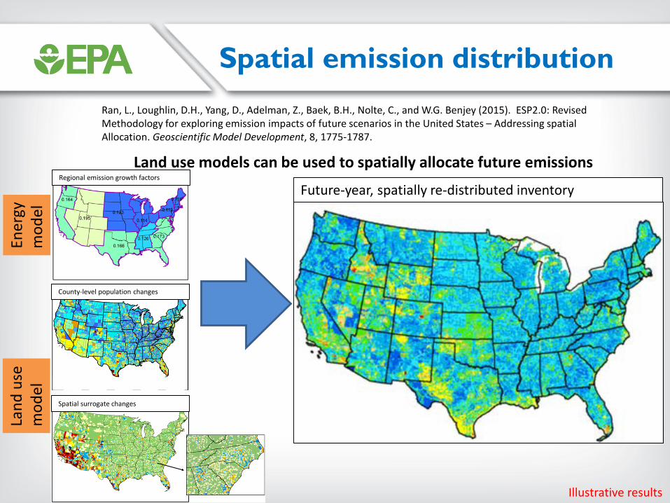
Spatial emission distribution
Illustrative results
Regional emission growth factors
County-level population changes
Spatial surrogate changes
Future-year, spatially re-distributed inventory
Ener
gym
odel
Land
use
mod
el
Ran, L., Loughlin, D.H., Yang, D., Adelman, Z., Baek, B.H., Nolte, C., and W.G. Benjey (2015). ESP2.0: Revised Methodology for exploring emission impacts of future scenarios in the United States – Addressing spatialAllocation. Geoscientific Model Development, 8, 1775-1787.
Land use models can be used to spatially allocate future emissions
Temporal emission distribution
Illustrative results
0
1
2
3
4
0 2000 4000 6000 8000
Elec
tric
ity p
rodu
ctio
n (P
J/hr
)
Electricity production 2010
Summer Fall Winter Spring
AMNight
Afternoon Peak
0
1
2
3
4
0 2000 4000 6000 8000
Elec
tric
ity p
rodu
ctio
n (P
J/hr
)
Electricity production 2050
Summer Fall Winter Spring
Energy model projections of technology and fuel use can inform temporal profiles
Winter 2010 2050
Morning 10% 10%
Afternoon 15% 16%
Peak 0.5% 0.4%
Night 2% 6%
Winter natural gas emissions by time of day (%) As natural gas takes on more of a baseload role, its night-time emissions share increases.
Available models, methods and tools
• Modeling– Optimization (How do I …?) e.g., NEMS (foresight mode), IPM, MARKAL– Simulation (What will happen if ...?) e.g., NEMS (myopic mode), GCAM-USA
• Techniques– Sensitivity analysis (response to incremental changes)– Scenario analysis (performance over very different conditions)– Modeling to Generate Alternatives (identification of very different pathways)
• Tools– Visualization– Statistics and data mining– Exploratory data analysis– Distributed computing– Software development and decision support systems– Integrated modeling frameworks 13
Air Quality FuturesObjective: Explore air quality management opportunities and challenges in the U.S. over a range of possible futures.Tool: MARKAL energy system optimization modelMethod: Future Scenarios MethodReference: Gamas, J., Dodder, R., Loughlin, D., and C. Gage (2015). “Role of future scenarios in understanding deep uncertainty in long-term air quality management.” Journal of the Air & Waste Management Assoc. doi 10.1080/10962247.2015.1084783.
Motivation
• Drivers of future pollutant emissions (and thus air quality) include: – Population growth and migration– Economic growth and transformation– Technology development and adoption– Climate change– Consumer behavior and preferences, and– Policies (energy, environmental, climate, …)
• As these drivers are uncertain, are there steps that we can take to:– understand a range of future conditions that may occur, – anticipate conditions that may limit the efficacy of air quality management
strategies, and,– develop management strategies that are robust over a wide range of future
conditions?
15
Future Scenario Method
• We applied the Future Scenarios Method to develop scenarios that inform air quality management decisions
• Future Scenarios Method steps:– Interview internal and external experts– Select the two most important uncertainties and develop a scenario matrix– Construct narratives describing the matrix’s four scenarios– Implement the scenarios into a model (MARKAL) and refine as necessary– Apply the scenarios to inform decision-making
Note: In this application, we developed a 2x2 scenario matrix. The method is adaptable, however, and could be used to develop more or fewer scenarios.
16
Future Scenario Method, cont’d
This is the resulting Scenario Matrix:
Conservation is motivated by environmental considerations. Assumptions include decreased travel, greater utilization of existing renewable energy resources, energy efficiency and conservation measures adopted in buildings, and reduced home size for new construction.
iSustainability is powered by technology advancements, and assumes aggressive adoption of solar power, battery storage, and electric vehicles, accompanied by decreased travel as a result of greater telework opportunities.
Muddling Through has limited technological advancements and stagnant behaviors, meaning electric vehicle use would be highly limited and trends such as urban sprawl and increasing per-capita home and vehicle size would continue.
Go Our Own Way includes assumptions motivated by energy security concerns. These assumptions include increased use of domestic fuels, particularly coal and gas for electricity production and biofuels, coal-to-liquids, and compressed natural gas in vehicles.
17
iSustainabilityConservation
Go Our Own Way
Muddling Through
Soci
ety
New Paradigms
Old and Known Patterns
Stag
nant
Transformation
Technology
Energy system model: MARKAL
18
• Bottom-up and technology-rich
– Captures the full system from energy resource supply/extraction technologies to end-use technologies in all sectors
– Energy technologies (existing and future techs) are characterized by cost, efficiency, fuel inputs, emissions
– Technologies are connected by energy flows
• Optimization
– The model picks the “best” way (lowest system-wide cost) to meet energy demands choosing from the full “menu” of energy resources and technologies
– The model makes these choices from 2005 to 2055, giving us a snapshot of possible future energy mixes
• Emissions and impacts
• All technologies and fuels have air and GHG emissions characterized
• Standards and regulations are included in the baseline, and additional policies can be modeled
U.S. EPA MARKAL regional database: EPAUS9r
• Coverage: U.S. energy system
• Spatial resolution: Nine Census divisions
• Modeling horizon: 2005 to 2055 in five year increments
• Pollutants: NOx, SO2, PM10, PM2.5, CO, VOC, CO2, CH4, N2O, BC, OC, water use for electricity generation
• Maintenance: Updated and calibrated to Annual Energy Outlook every two years; housed at EPA/ORD; publicly available
Scenario implementation
• Implementation of the scenarios was a learning process
• Early approach:
– Developed highly detailed narratives– Constrained MARKAL to follow the detailed narratives – Advantage: The scenarios differed considerably with respect to
projected technology penetrations and air pollution emissions.– Disadvantage: The scenario assumptions were hard-coded, leaving
the model little freedom to respond to a policy or other “shocks”. • Current approach:
– Step back from the detailed narratives and focus on underlying drivers
– Let the model drive the narratives
20
• Current approach
– Axis: Technological transformation or stagnationLever: technological availability and cost
Scenario implementation, cont’d21
No electric vehiclesNo IGCC
No electric vehiclesNo IGCC
Electric vehicles achievecost parity with conventional
Solar costs are reduced (obtained from IPM v5.15)
Only consideredtechnologies thatare competitive todaywithout subsidies
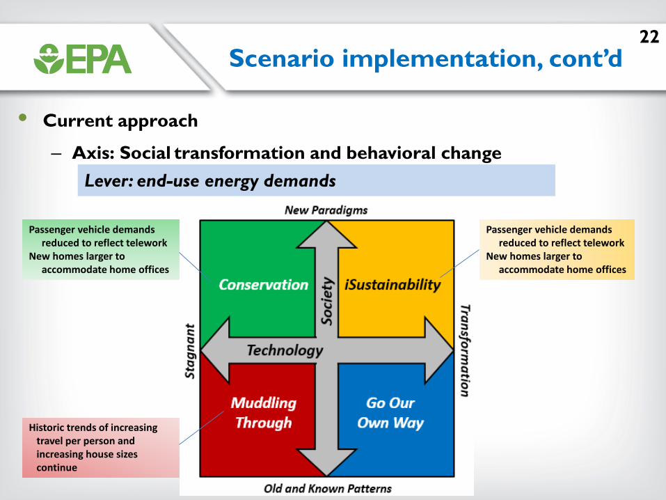
• Current approach
– Axis: Social transformation and behavioral changeLever: end-use energy demands
Scenario implementation, cont’d22
Passenger vehicle demands reduced to reflect telework
New homes larger to accommodate home offices
Historic trends of increasingtravel per person andincreasing house sizescontinue
Passenger vehicle demands reduced to reflect telework
New homes larger to accommodate home offices
• Current approach
– Axis: Social transformation and behavioral changeLever: hurdle rates to reflect scenario-specific preferences
Scenario implementation, cont’d23
Prefer:RenewableEnvironmental- and
climate-friendlyLocalEnergy efficient
Prefer:Conventional technologies
Avoid:Advanced technologiesInfrastructure changes req’dEnvironmental- and
Avoid:Infrastructure changes req’dHigh capital cost
Illustrative results
How different are the scenario results?
What are the long-term emission trends and how do they differ by region?
How effective are existing regulations at controlling emissions over wide-ranging scenarios of the future?
24
Illustrative results, cont’dHow different are the scenario results?
Electricity production by aggregated technologies
25
Coal
Gas
Nuclear
Solar
Wind
Light duty vehicle technologies
26Illustrative results, cont’dHow different are the scenario results?
E85
Conventional
Electric
Hybrids& pluginhybrids
Historic SO2 reductions are “locked in”but there is a small amount of variability.
EmissionsCAIR and Tier-3 drive NOx trend Greatest variability in CO2
Existing regulations are relatively robust in locking in downward trends for criteria pollutants.
The range of CO2 emissions across the scenarios is considerably greater than that of the other pollutants.
27Illustrative results, cont’dWhat are the long-term emission trends?
Decision support system
Project: GLIMPSEObjective: Provide decision support framework for evaluating state-level energy, environmental, and climate management leversRequirements: Address decision-relevant sectors and time horizons, state-level resolution, easy to use, freely available
ORD’s GLIMPSE project
GoalDevelop analytical tools for:
• Evaluating how candidate management strategies meet environmental, climate and energy objectives
• Characterizing tradeoffs among objectives
• Identifying strategies that efficiently meet all objectives
29
Meetsclimate
objectives
Meetsenvironmental
objectives
Meetsenergy
objectives
Management strategy space
Why GCAM-USA?
• GCAM track record – USGCRP, IPCC, EMF …
• Spatial coverage and resolution– Global, covering U.S. at state-level
• Time horizon and resolution– 2005-2100 in 5-year time-steps
• Sectoral coverage– Energy, land use, agriculture, water, climate
• Pollutant coverage– GHGs and many criteria pollutants (e.g., NOx, SO2, PM, NH3, CO)
• Technological representation– Highly resolved compared to most Integrated Assessment Models
• Other– Free, open source, user community, no specialized software or equipment,
structure is amenable to addition of graphical user interface30
Why GCAM-USA?
31
GCAM Components
GCAM-USA modifications FY16
• Emission factor updates
• Regulatory representations
32
Sector Source
Electric IPM version 5.14
Industrial GREET, Regulatory Impact Analyses
Residential/commercial Webfire database
Highway vehicles MOVES 2014
Non-highway vehicles NONROAD, various Regulatory Impact Analyses
Regulation Summary
Cross-State Air Pollution Rule State-level, electric sector NOx and SO2 caps
Clean Power Plan State-level, electric sector CO2 caps
CAFE National light duty vehicle efficiency requirements
Tier 3 Emission standards for highway vehicles
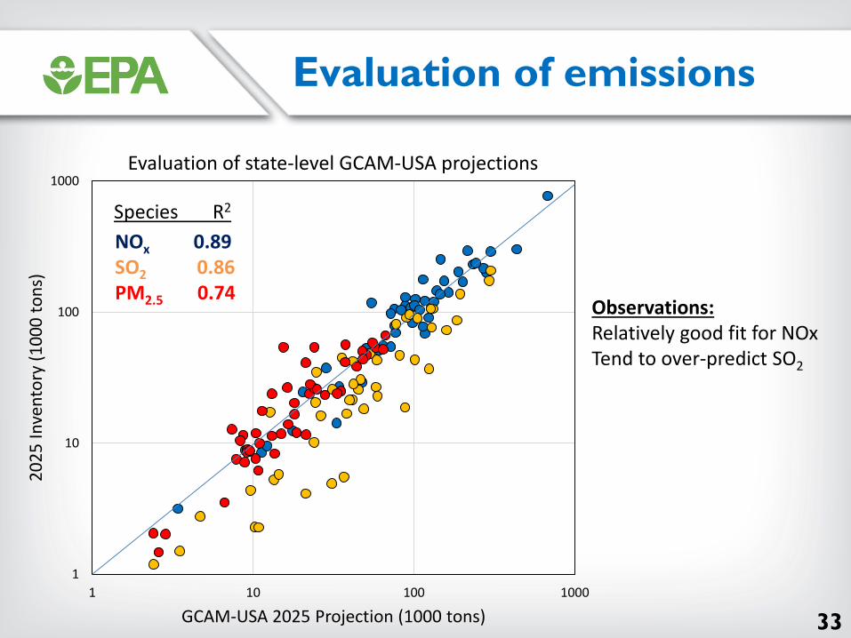
Evaluation of emissions
33
1
10
100
1000
1 10 100 1000
2025
Inve
ntor
y (1
000
tons
)
GCAM-USA 2025 Projection (1000 tons)
Evaluation of state-level GCAM-USA projections
NOx 0.89SO2 0.86PM2.5 0.74
Observations:Relatively good fit for NOxTend to over-predict SO2
Species R2
34
NOx emissions (tons x1000)compared to EPA 2011eh platform
• Off-highway NOx is low relative to the inventory, but this could be because of discrepancies in what is being compared
• Industrial sector SO2 from GCAM-USA are two times higher than the inventory. A hypothesis we are testing is that offroad mobile emissions included GCAM’s industrial sector may not reflect mobile source fuel sulfur content limits. We also need to examine the assumed mix of industrial boilers, turbines, and engines in GCAM-USA.
SO2 emissions (tons x1000)compared to EPA 2011eh platform
Evaluation of emissions, cont’d
Potential applications
Examples of policy levers that could be evaluated with GCAM-USA:• Types
– Air pollutant taxes or caps– GHG taxes or caps– Technology subsidies– Forced technology penetration– High-efficiency technology end-use requirements– CAFE standard– Renewable Electricity Standard
• Geographic application– Global, global region, or national– Group of states or individual state
35
Illustrative application:– 50% Renewable Energy Standard
introduced from 2025, applied to Texas– Applies to annual electricity production
from new builds in each state
36
RES application
37
0.0
0.5
1.0
1.5
2.0
2.5
3.0
3.5
4.0
2010 2015 2020 2025 2030 2035 2040 2045 2050
EJ Texas, 50% RES target
0.0
0.5
1.0
1.5
2.0
2.5
3.0
3.5
4.0
2010 2015 2020 2025 2030 2035 2040 2045 2050
EJ Texas, Base Case
-2.0
-1.5
-1.0
-0.5
0.0
0.5
1.0
1.5
2.0
2010 2015 2020 2025 2030 2035 2040 2045 2050
EJ 50% RES – Base Case
0%
20%
40%
60%
80%
100%
120%
140%
160%
2010 2015 2020 2025 2030 2035 2040 2045 2050
Emission metrics relative to 2010Dashed - Base Case; Solid - 50% RES
CO2 NOx SO2 PM mortality
Electricity production by aggregated technology
Observations:• A 50% RES (for new builds) in Texas reduces electricity
production from coal and gas, which are displaced largely by wind
• This transition yields reductions of CO2, NOx, SO2, and PM mortality costs
Note: The Clean Power Plan is not included in these results
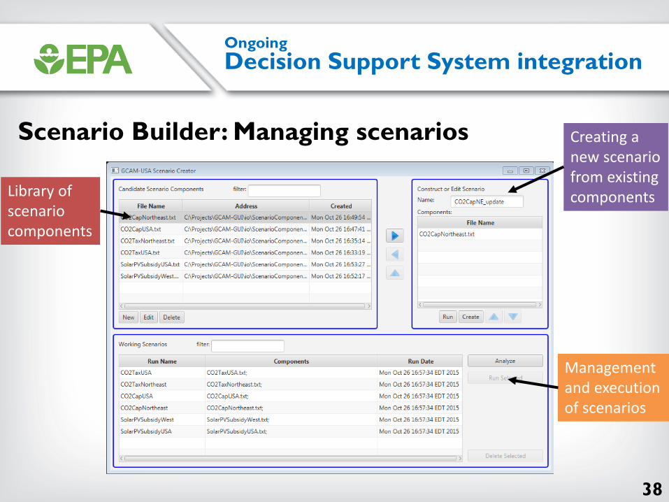
OngoingDecision Support System integration
38
Scenario Builder: Managing scenarios
Library ofscenariocomponents
Creating anew scenariofrom existingcomponents
Managementand executionof scenarios
OngoingDecision Support System integration
39
Enhancements to the Model Interface
Show results separate plots
Easily sum overregions and est-imate differencesacross scenarios
Choose from line, bar, and pie charts
Concluding remarks
• This presentation touches on a handful of ways in which the U.S. EPA Office of Research and Development is working to explore how air quality management and greenhouse gas mitigation goals can be met more cost-effectively and robustly
• EPA has many internship and post-doctoral opportunities that may be of interest to current and graduating students
• There may be opportunities for collaboration with the ACE Centers, including the one in which JHU is participating
40
Questions?Contact information: Dan Loughlin, U.S. EPA, ORD – [email protected]
Processing and Conversion of Energy Carriers End-Use Sectors
Conversion & Enrichment
Processing & conversion of energy carriers
Fossil fuels
Biomass
Uranium
Wind, solar &hydro resources
Conversion & enrichment Nuclear power
H2 production
Fossil fuels
Primaryenergy
Processing and conversion End-use sectors
Biomass
Uranium
Wind, solar and hydro resources
Refining and processing
Transportation
Residential
Commercial
Industrial
Gasification
Carbonsequestration
Combustion
Conversion andenrichment
Renewable electricity
Electric Grid
Transmission
Components of the energy system
Why the energy system?
45
Energy system contributions to environmental concerns: • Air quality1
– Photochemical smog: 92% of nitrogen oxide (NOx) emissions*– Acid rain: 90% of sulfur dioxide (SO2) emissions*
• Climate change2
– Greenhouse gas emissions: 95% of carbon dioxide (CO2) emissions* – Major source of short-lived climate pollutants (e.g., black carbon, methane)
• Water – Demands: electricity production accounts for 45% of U.S. water withdrawals3
– Pollution: • wastewater from fuel extraction and processing, seepage from waste • eutrophication from N deposition, acidification from S and N deposition
*Percentage of U.S. anthropogenic emissions from the energy system in 2014
1 EPA trends report
2 EPA 2016 GHG Inventory
3 Maupin et al., 2014 (USGS)
Models
46
Attribute NEMS IPM EPA MARKAL GCAM-USA
Type Simulation or Optimization Optimization Optimization Simulation
Formulation
Many modules, some of which are linear, nonlinear, mixed integer, etc
Linear or mixed-integer linearprogramming
Linear or mixed-integer linearprogramming Dynamic, recursive nonlinear
ForesightMyopic or Perfect (withcomputational penalty) Perfect Perfect Myopic
SpatialU.S. Census Division, NERCregion NERC region and state-level U.S. Census Division Global and state-level
Temporal2015-20401-year time step
2016-2050configurable time step
2005-20555-year time step
2010-21005-year time step
Sectoral
Energy system (Electricity,industry, residential, commercial, transportation) Electricity production
Energy system (Electricity,industry, residential, commercial, transportation)
Energy, plus agriculture, land use, climate, and water
Technologies Very high number Medium number High number Medium number
Demand elasticity Yes
Electricity demands are elastic to price
Optional, currently not used because of computational penalty Yes
RuntimeApproximately half-day on computational server
Several hours on computational server
1 hour on typical desktop computer
1 hour on typical desktop computer
AvailabilitySpecial software required, economic model proprietary Proprietary
Special software required, model is proprietary
Open source, no specialsoftware required
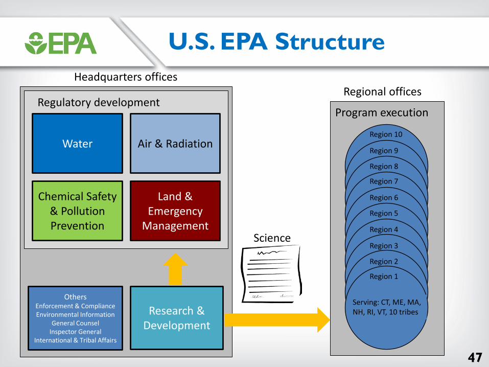
U.S. EPA Structure
47
Regional officesHeadquarters offices
Research & Development
Water Air & Radiation
Chemical Safety & Pollution Prevention
Land & Emergency
Management
OthersEnforcement & ComplianceEnvironmental Information
General CounselInspector General
International & Tribal Affairs
Regulatory developmentProgram execution
Science
Region 10
Region 9
Region 8
Region 7
Region 6
Region 5
Region 4
Region 3
Region 2
Region 1
Serving: CT, ME, MA,NH, RI, VT, 10 tribes
Technology assessmentObjective: Explore the role that centralized solar photovoltaics (CSPV) can play in CO2 mitigationTool: MARKAL energy system optimization modelMethod: Nested sensitivity analysisReference: Loughlin, D., Yelverton, W., Dodder, R., and C. A. Miller (2012). “Examining potential technology breakthroughs for mitigating CO2 using an energy system model.” Clean Technologies and Environmental Policy. doi:10.1007/s10098-012-0478-1. Mar. 27, 2012.
MARKALenergy system
linear programming model
Scenario assumptions
Population growth andmigration
Economic growth and transformation
Climate change impactson heating and cooling
Technology development
Behavior and preferences
Policies
Outputs
Energy-related technology penetrations and fuel use
Emissions• air pollutants• GHGs• short-lived climate
pollutants (SLCPs)
Water demands
1st order estimates ofhealth and warmingimpacts
EPA MARket ALlocation (MARKAL) modeling framework
Objective: Select the technologies and fuels that minimize net present value over the 50-year modeling horizon
Time horizon: 2005 – 2055; Temporal resolution: 5 years; Spatial coverage: U.S.; Spatial resolution: Census Division
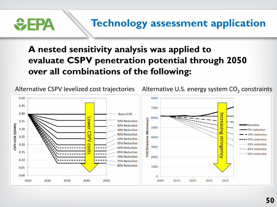
A nested sensitivity analysis was applied to evaluate CSPV penetration potential through 2050 over all combinations of the following:
50
Technology assessment application
Lower CSPV costs
Increasing stringency
Alternative CSPV levelized cost trajectories Alternative U.S. energy system CO2 constraints
51
Technology assessment application
Electricity output (billion kWh) from CSPV in 2050Results:
Insights:• For the 30% mitigation targets, CSPV penetration followed the expected trends• Counter-intuitively, increasing the CO2 reduction target to 40% or 50% reduced CSPV output• Further analysis suggested:
– the more stringent reduction targets led to electrification of end uses (e.g., vehicles and building heating systems)
– these changes disproportionately led to more night-time electricity demands– other technologies respond better to nighttime demands (e.g., nuclear, wind, coal and gas with
CCS)
Ongoing:• Exploring vehicle time-of-charging assumptions, stationary storage, and regional considerations