Analytical Biochemistry, in press ON THE ANALYSIS … · Analytical Biochemistry, in press ON THE...

Analytical Biochemistry, in press

ON THE ANALYSIS OF PROTEIN SELF-ASSOCIATION BY

SEDIMENTATION VELOCITY ANALYTICAL ULTRACENTRIFUGATION

Peter Schuck

Protein Biophysics Resource, Division of Bioengineering & Physical Science, ORS, OD, National

Institutes of Health, Bethesda, Maryland 20892.

Running Title: PROTEIN SELF-ASSOCIATION

Keywords: protein interactions, reversible associations, Lamm equation, sedimentation

equilibrium

Category: Physical Techniques Author’s Address: Dr. Peter Schuck National Institutes of Health Bldg. 13, Rm. 3N17 13 South Drive Bethesda, MD 20892-5766,USA Phone: 301 435-1950 Fax: 301 480-1242 Email: [email protected]

2

ABSTRACT

Analytical ultracentrifugation is one of the classical techniques for the study of protein interactions and

protein self-association. Recent instrumental and computational developments have significantly

enhanced this methodology. In the present paper, new tools for the analysis of protein self-association

by sedimentation velocity are developed, their statistical properties are examined, and considerations

for optimal experimental design are discussed. A traditional strategy is the analysis of the isotherm of

weight-average sedimentation coefficients sw as a function of protein concentration. From theoretical

considerations, it is shown that it integration of any differential sedimentation coefficient distribution

c(s), ls-g*(s), or g(s*) can give a thermodynamically well-defined isotherm, as long as it provides a

good model for the sedimentation profiles. To test this condition for the g(s*) distribution, a back-

transform into the original data space is proposed. Deconvoluting diffusion in the sedimentation

coefficient distribution c(s) can be advantageous to identify species that do not participate in the

association. Because of the large number of scans that can be analyzed in the c(s) approach, its sw

values are very precise and allow extension of the isotherm to very low concentrations. For all

differential sedimentation coefficients, corrections are derived for the slowing down of the

sedimentation boundaries caused by radial dilution. As an alternative to the interpretation of the

isotherm of the weight-average s-value, direct global modeling of several sedimentation experiments

with Lamm equation solutions is studied. For this purpose, a new software SEDPHAT is introduced,

allowing the global analysis of several sedimentation velocity and equilibrium experiments. In this

approach, information from the shape of the sedimentation profiles is exploited, which permits the

identification of the association scheme, and requires fewer experiments to precisely characterize the

association. Further, under suitable conditions, fractions of incompetent material that are not part of

the reversible equilibrium can be detected.

3

Introduction

It has become increasingly obvious that reversible interactions of proteins are among the fundamental

principles that govern their role and organization. Reversible self-association is one of the more

intricate, yet ubiquitous modes of interactions. Self-association is frequently coupled to heterogeneous

protein-protein interactions, and often represents an integral part of the reaction mechanism. This

highlights the importance of methods that allow the characterization of the thermodynamic properties

of self-associating proteins in solution. Among the classical techniques of physical biochemistry for

studying protein association is analytical ultracentrifugation (1, 2) (for recent reviews, see, e.g., (3-8)).

In the 1990s, the technique has experienced a renaissance (see, e.g. (8-12)), largely due to the ability to

study reversible interactions in solution and the increasing interest in protein interactions.

The present paper is concerned with two sedimentation velocity approaches – the method of

isotherms of weight-average sedimentation coefficients and the analysis of the shape of the

sedimentation boundary. They focus on different aspects of the experiment and have evolved in

parallel. To understand their relationship, it is of interest to follow their historical development.

Already in the 1930s, evidence for reversible protein interactions measured by sedimentation velocity

was reported (1). Following were more systematic studies of the concentration-dependence of the

sedimentation coefficient, interpreted in the context of protein self-association. These include, for

example, studies of α-chymotrypsin (13, 14), insulin at low pH (15), casein (16), hemoglobin (17) and

others (2). In parallel, the theoretical framework of sedimentation velocity of self-associating systems

was rapidly developed. From the work of Tiselius, it was known that in moving boundary transport

experiments no resolution of boundaries will occur if the components are in a rapid equilibrium

compared to the rate of migration, in which case a weight-average migration velocity will be observed

(18). In the 1950s, Baldwin has shown that the migration of the second moment position of the

sedimentation boundary corresponds to the weight-average s-value of the solute composition in the

4

plateau region (19), which was related to the chemical equilibrium (via mass action law) between

monomeric and oligomeric species by Oncley et al. (15) and Steiner (20).

With regard to the shapes of the sedimentation boundary, Gilbert examined the ideal case of

negligible diffusion and fast chemical rates. He quant itatively predicted the features of such ‘ideal’

boundaries and found qualitative differences between monomer-dimer and higher self-association

schemes (21). Examples for the application of Gilbert theory are the self-association of α-

chymotrypsin (22) and β-lactoglobulin (23). It was also applied by Frigon and Timasheff in the

detailed analysis of the ligand- induced self-association of tubulin, which also included hydrodynamic

models of the oligomers (24, 25) (a topic reviewed by Cann (26)). Since then, the analysis of protein

self-association by the concentration dependent weight-average sedimentation coefficients, sometimes

combined with hydrodynamic models and qualitative interpretation of the boundary shape has been

applied in many studies (27-33) and others (for a recent review of this approach, see (34)).

As pointed out by Fujita, the diffusion-free approximation of Gilbert-theory represents a limitation

in the interpretation of actual data (35). This was overcome with numerical solutions of the Lamm

equation (the transport equation describing the coupled sedimentation and diffusion process (36)) (37-

42), which was also extended to kinetically controlled self-associations and applied to hetero-

associations (43-46). Numerical or approximate analytical Lamm equation solutions coupled with

non- linear regression can now be used routinely to model experimental data (40, 41, 47-51). Algebraic

noise decomposition permits direct modeling of the interference optical data by calculating the time-

invariant and radial- invariant signal offsets (52). This allows to take full advantage of the excellent

signal-to-noise ratio of the laser interferometry detection system, and, similarly, to perform separate

experiments in each sector of the centrifugal cell when using the absorbance scanner (53). In recent

years, some experience with modeling Lamm equation solutions for self-associating proteins to

experimental data has been gained (32, 41, 54-59). While the importance of globally modeling

5

experiments from different loading concentrations has become clear, a more systematic study of useful

experimental conditions, analogous to those available for sedimentation equilibrium studies (for

example, (60-63) and others) is still lacking.

Modern computational techniques have also led to considerable improvements in the

determination of weight-average sedimentation coefficients via differential sedimentation coefficient

distributions, which have the potential to discriminate different sedimenting species. In 1992, Stafford

has shown how an apparent sedimentation coefficient distribution g(s*) can be calculated from a

transformation of the time-derivative of the sedimentation profiles (64, 65). This approach allows to

extract information from many scans at once, and due to the use of pair-wise differencing is well

adapted to the time- invariant noise structure of the interferometric detection system. It has been

widely used, and was reviewed in the context of weight-average s-values by Correia (34). More

recently, it was shown how an apparent sedimentation coefficient distribution ls-g*(s) can be

calculated directly from least-squares modeling of the sedimentation profiles, permitting higher

precision through the use of an increased data basis and permitting wider distributions and more

general application (66). A sedimentation coefficient distributions c(s) with significantly higher

resolution can be achieved through direct modeling and deconvolution of diffusional broadening of a

complete set of sedimentation profiles (67-69). In general, differential sedimentation coefficient

distributions are particularly powerful for more complex protein interaction processes. Recent

examples include the ligand- induced self-association of tubulin (58 , 70), amyloid formation (71) and

entanglement of amyloid fibers (72) and others (33, 54, 73, 74).

Despite the obvious utility of the sedimentation coefficient distributions, some theoretical and

practical aspects still have to be examined. For example, it is unclear how they relate to a

thermodynamically well-defined weight-average sedimentation coefficient, and from which

experimental data sets they may be derived. In this regard, the ls-g*(s) and c(s) distribution are of

6

particular interest as they apply Bayesian principles such as maximum entropy regularization for

selecting the most parsimonious distribution consistent with the raw data. Also, the increased

precision of the experimental sedimentation data warrants a more detailed study of the effect of

boundary deceleration caused by the radial dilution of the sample in the sector-shaped ultracentrifuge

cell, and how this applies to the different sedimentation coefficient distributions.

These topics are addressed in the present paper. It analyzes and compares the two major strategies

for characterizing protein self-association by modern sedimentation velocity, which are the

determination of an isotherm of weight-average sedimentation coefficients as a function of protein

concentration and global non- linear regression of the sedimentation data with Lamm equation models.

A practical example of the latter approach will be published in the context of the biophysical

characterization of the self-association of gp57A of the bacteriophage T4 (59). Several new tools are

introduced for both strategies. Although the present work focuses on the analysis of protein self-

association, most of the conclusions will also apply to the study of heterogeneous protein interactions

(after accounting for different signal contributions of the different species).

Theory and Modeling

Weight-average sedimentation coefficients for concentration dependent solutes

In this section, first, the definition and theoretical relationships underlying weight-average

sedimentation coefficients sw are recapitulated. This will lead to a new definition of an ‘effective’

concentration c* for interpreting sw(c*) of rapidly equilibrating concentration dependent systems when

sw is derived from sedimentation coefficient distributions. It will also lead to the result that sw can be

obtained by integration of the recently described differential sedimentation coefficient distribution c(s)

and ls-g*(s). Importance is given to the experimental conditions required for the practical application.

The evolution of the concentration distribution throughout the sector-shaped cell for a single

ideally sedimenting species with sedimentation coefficient s and diffusion coefficient D is described by

7

the Lamm equation

2 21c cs r c Dr

t r r rω

∂ ∂ ∂ = − − ∂ ∂ ∂ (1)

(36). For a sedimenting boundary that exhibits a plateau, i.e., a vanishing concentration gradient

( ) 0pc r r∂ ∂ = at a plateau radius value rp (non-standard loading configurations are excluded), the

multiplication of Eq. 1 with r and integration over the radial coordinate from the meniscus rm to the

plateau at rp gives

2 2 2 2( , ) ( ) ( ) ( )p

m

r

p p p w p p pr

dc r t rdr s c r c t s c r c

dt− = ω ≡ ω∫ (2)

(Eq. 2.229 p. 116 in (35)), where s(cp) is the sedimentation coefficient at the plateau concentration cp at

rp. As illustrated by Schachman (2) (p. 65), the left-hand side describes the loss of mass of

sedimenting material between meniscus and the plateau region, due to transport flux through an

imaginary cross-section of the solution column at rp. For sedimenting multi-component mixtures, this

total flux is used to define the weight-average sedimentation coefficient sw. It should be noted that this

definition is completely independent of the boundary shape. Important in practice is that, because of

the vanishing flux at the meniscus, the definition of sw via integration of Eq. 2 does not require the

meniscus region to be depleted, in contrast to the alternate derivation in (3).

It is of theoretical and practical interest to study how sw relates to the displacement of the

sedimentation boundary. According to the second moment method, the mass balance integral in the

definition of sw (r.h.s. of Eq. 2) can be expressed by an equivalent boundary position rw of a single non-

diffusing species with sedimentation coefficient sw(cp) (2, 35), with

∫−=p

m

r

rppw rdrtrc

crtr ),(

2)( 22 (3)

(Eq. 11 in (2)). With a slight modification of the derivations by Fujita (35) an explicit expression of

8

the weight-average sedimentation coefficient can be derived as

+

−−

ω−== ∫

p

m

r

rppw

m

ppw

mpmpww rdrtrc

crr

r

crr

rrr

dtd

css ),(2)(

1log2

1)(* 22

2

22

222

2

(4)

An analogous expression is given by Fujita (Eq. 2.234 in (35)) and was derived by Baldwin (19), using

an integral over the concentration gradient. Similar to Eq. 2, in Eq. 4 the weight-average

sedimentation coefficient sw at the plateau is related with the total depletion of material between

meniscus and an arbitrary plateau radius rp. This depletion can be calculated directly from each scan at

different times t, and is independent of the boundary shape. The weight-average sedimentation

coefficient is taken at the plateau concentration at the time of the scan (19). It should be noted that Eq.

4 only considers the instantaneous rate of transport across a boundary, and is therefore completely

independent of the history of the concentration distribution or the meniscus position. It only requires

the transport at the times considered to be a result of free sedimentation.

For the present purpose of calculating sw for a concentration-dependent system from

sedimentation coefficient distributions (e.g. c(s) (67), ls-g*(s) (66) and g(s*) (64, 65)), it is useful to

bring Eq. 4 into a different form. The reason is that these sedimentation coefficient distributions are

based on equations that imply the entire sedimentation process from the start of the centrifugation

experiment, rather than the change in mass balance only at the time of the scans. This is also true for

the dcdt method to obtain g(s*), as the differential is only used to eliminate the constant signal offsets.

Therefore, we integrate Eq. 4 with respect to the time from 0 to the time T (the time of the scan

considered), which gives

0

2 2 2 2

2 2 2 2 2

1* ( ( ))

( ) 21log 1 ( , )

2

p

m

T

w w p

rm p m m

w p p w p p r

s s c t dtT

r r r rc r t rdr

T r r c r r cω

=

− = − − +

∫

∫ (5)

9

If the sedimentation coefficient is concentration independent, sw* equals sw. For concentration-

dependent sedimentation, however, sw* is only an apparent weight-average sedimentation coefficient

that, strictly, is not a constant because the radial dilution changes the plateau concentration and results

in corresponding changes in the chemical composition (1, 35). This also implies a dependence on the

reaction kinetics of the system.

The difference between Eq. 4 and 5 can be illustrated, for example, with a rapid self-associating

monomer-n-mer system in the limit of an infinite solution column. Because of the radial dilution, with

time such a system would completely dissociate and the weight-average sedimentation coefficient sw

from Eq. 4 would assume the monomer s-value. Nevertheless, if transforming the boundary position

r(t) into an apparent s-value s* (such as in the g*(s) method (64)), this transformation would also

reflect the period when the molecules migrated as the assembled species. This is taken into account in

Eq. 5. For typical experimental conditions, radial dilution amounts only to ~ 20-30%, and

corresponding changes in sw are generally small. However, they can be distinctly larger than the

measurement error, and the corresponding systematic changes in sw* have been noted already by

Svedberg (1).

We suggest an approximate correction for the case that the change in sw(c) is not kinetically

limited and can be approximated over a small concentration range as a linear function of concentration.

In this case, we can separate sw from the time integral in Eq. 5

0

* ( ) ( * ( ))

1* ( ) ( )

w w

T

p

s T s c T

c T c t dtT

≅

= ∫ (6)

The average plateau concentration from time 0 to T can be calculated using the Lamm equation in the

absence of concentration gradients

ppwp ccsdt

tdc 2)(2)(

ω−= (7)

10

which leads to

( )2202*( ) 1

2ws T

w

cc T e

s Tω

ω−= − (8)

This means that for systems that locally approach chemical equilibrium faster than the time-scale of

sedimentation, the measured apparent weight-average sedimentation coefficient sw* from a sample

with loading concentration c0 is a good approximation of the true weight-average sedimentation

coefficient at a reduced concentration c*. (For analysis of multiple scans at different Ti, the average of

all c*(Ti) should be taken). For slow equilibrating systems, however, sw* will reflect the equilibrium

composition at loading concentration c0. For systems with unknown kinetics, it is possible to assign

the concentration an uncertainty from c0 to c*, and to analyze the isotherm sw(c) by treating the c-

values as unknowns within these bounds.

It is possible to generalize the above treatment to a general mixture of k reacting components. In

this case, the Lamm equation can be extended by local reaction fluxes qk (35). One can still define the

weight-average sedimentation coefficient in a similar way by considering the evolution of the total

concentration

2 2,

2 2,

( , )

( )

p

m

r

tot p k k p kk kr

w p p p tot

dc r t rdr r s c q rdr

dt

s c r c

= − ω +

≡ − ω

∑ ∑∫ ∫ (9)

As long as the total signal from the chemical reaction is conserved (throughout the observed region

from meniscus to rp) it is 0=∑k kq , and the extra term in Eq. 9 is identically zero. Therefore, we

arrive again at a weight-average sedimentation coefficient

∑

∑=

kpk

kpkk

pkw c

cs

cs,

,

, )( (10)

that reflects only the weighted average of the s-values of the composition at the plateau. This shows

11

that sw is not affected by chemical equilibria or reaction kinetics, except to the extent of the problem

arising from decreasing plateau concentrations discussed above.

Its current practice to determine the weight average sedimentation coefficients not from the mass

balance and integration of the sedimentation boundary, but from differential sedimentation coefficient

distributions c’(s), which are defined as a superposition of independently sedimenting species

∫= dstrsctrctot ),,('),( (11)

Since the evolution of ctot is described by a superposition of Lamm equations, the definition of sw can

be obtained by extension of Eq. 2

2 2 2 2,( , ) ' ( )

p

m

r

tot p p w p p pto tr

dc r t rdr r sc ds s c r c

dtω ω− = ≡∫ ∫

(12)

with cp’ denoting the differential sedimentation coefficient distribution at the plateau (2). If each

species of the distribution c’(s) sediments independently of concentration, which is assumed in all

currently known sedimentation coefficient distributions, it follows that in the plateau cp’(s) ~ c’(s) and

∫∫=

dsc

sdsccs pw

'

')( (13)

, i.e., the weight-average sedimentation coefficient can be calculated by integrating the differential

sedimentation coefficient distribution.

It should be noted that the diffusion coefficient does not occur in Eq. 12, so that the result Eq. 13

is equally valid for any differential sedimentation coefficient distributions, independent of diffusion.

This includes c(s) (67, 68), ls-g*(s) (66) and g(s*) from dcdt (64, 65). Another consequence of this is

the invariance of the sw value obtained from the c(s) distribution calculated with any value of f/f0 (or

other prior knowledge). The only requirement is that the distribution provides a good description of

mass balance between meniscus and rp, for which a good fit of the sedimentation boundary (i.e. the

experimentally observed sedimentation profiles) is sufficient. Similarly, when modeling sedimentation

12

data of an interacting system empirically with a size-distribution, a good fit (and ident ical mass

balance) is also sufficient for the sw value from Eqs. 12 and 13 to be identical to the correct weight-

average sedimentation coefficient of the interacting system. However, sw may still depend on the

plateau concentration cp and represent only an apparent weight average sedimentation coefficient sw*

as described above. In contrast, the integral sedimentation coefficient distribution G(s) (75) does not

lend itself to the mass balance considerations because it considers the boundary profiles only

normalized relative to the plateau level. The same result holds for the integral sedimentation

coefficient distributions G(s) when calculated from the extrapolation of ls-g*(s) to infinite time (68).

Because a large number of scans covering an extended time period of the sedimentation process

can be analyzed with ls-g*(s) and c(s), and because c(s) can be applied to a variety of experimental

conditions and lead to a high resolution of small species, it is worthwhile to reconsider the assumptions

under which the (apparent) weight-average sedimentation coefficient was defined. No depletion at the

meniscus is required. In principle, a solution plateau needs to be established for sw to represent a

meaningful quantity, since if there were concentration gradients, diffusion fluxes will artificially

increase or decrease the sw values. On the other hand, if a plateau can be established in the first several

scans under consideration, and if the corresponding sedimentation boundaries are modeled well,

extension of the time range to include later scans will leave the sw value invariant. Such extension may

increase the resolution in the sedimentation coefficient distribution, for example, for the identification

of slowly sedimenting species contributing to sw. However, if the definition of Eq. 13 is used for

calculating an sw value on the basis of a sedimentation coefficient distribution, the integration range

should be limited to species that do not exhibit significant back-diffusion. Otherwise, the

corresponding concentration will be ill-defined and the uncertainty may become much larger than the

range from c0 to c* indicated above.

In summary, it is shown above that integration of any of the differential sedimentation coefficient

13

distributions can be used to calculate sw, under the condition that a good model of the sedimentation

profiles is achieved. For interacting systems, the relevant concentration is not the plateau

concentration. For systems with a slow kinetics relative to sedimentation, it is the loading

concentration, while for fast reversible systems it is the effective time-averaged plateau concentration

c* (Eq. 6). sw is independent of the boundary shape, but requires that the sedimentation process is free

of convection for the entire experiment. The meniscus does not need to be cleared, and sw can be

determined from experimental data that do not exhibit plateaus throughout, but integration of the

sedimentation coefficient distribution over species that exhibit back-diffusion should be avoided for

interacting systems.

Data analysis

For the data analysis based directly on the second moment, Eqs. 4, 5 and 8 were implemented in the

software SEDFIT (combined with routines extracting a stable least-squares estimate of cp for each

scan). For both the differential (Eq. 4) and the integral form (Eq. 5) the average values for sw are

calculated, and the corresponding radial dilution factors (i.e., the plateau concentrations or c* (Eq. 8))

are also averaged for all scans considered in the analysis.

The differential sedimentation coefficient distributions c(s) (67) and ls-g*(s) (66), which are based

on direct models of the sedimentation data with Lamm equation solutions with and without the

deconvolution of diffusion, respectively, were also calculated with SEDFIT. In brief, in the c(s)

method the concentration distributions of a single noninteracting species χ(s,D,r,t) is calculated by the

Lamm equation Eq. 1 for a large number of sedimentation coefficients ranging from smin to smax. For

each s-value, the corresponding diffusion coefficient is estimated from a weight-average frictional ratio

(f/f0)w as

( )( ) ( )( )3 2 1 21 20

2( ) 1

18 wD s kT s f f v vη ρ

π− −−= − (14)

14

(69). The best- fit distribution c(s) is determined by a linear least-squares fit to the experimental data

a(r,t)

max

min

( , ) ( ) ( , ( ), , )s

s

a r t c s s D s r t dsχ≅ ∫ (15)

This Fredholm integral equation is stabilized with additional constraints derived from maximum

entropy or Tikhonov-Phillips regularization, which provides the simplest distribution that is consistent

with the available data (69). The extent of regularization is scaled by a statistical criterion to ensure

that the decrease of the fit quality imposed by the constraint is not significant on a one standard

deviation confidence level. The value for the weight-average frictional ratio (f/f0)w is determined

iteratively from the experimental data by a non- linear regression, which also may include the precise

meniscus position of the solution column (68). An analogous procedure with constant D = 0 is used

for calculating the apparent sedimentation coefficient distribution ls-g*(s) (66). Corrections for the

solvent compressibility are available (42).

The g(s*) distributions based on the time-derivative method were calculated with the software

DCDT+ (J.S. Philo, 3329 Heatherglow Ct., Thousand Oaks, CA 91360) (65). A transformation of the

so calculated g(s*) into a direct model of the sedimentation profiles was included as a function in

SEDFIT, by building a step-function model as described in (66) from the data exported from g(s*). In

order to rebuild the degree of freedom from the differencing of pair-wise scans in dcdt, the

sedimentation model can be combined with systematic noise calculation as described in (52, 68).

The isotherm of the weight-average sedimentation coefficient for a self-associating system can be

written as (24)

0,1

, 1

0, 1

( )1

11

i iw tot i toti

i s i i

ii i tot

s tot i

ss c K c c

k K c

s K c ck c

=+

≅+

∑

∑ (16)

15

where s0,i are the species sedimentation coefficients at infinite dilution, ks,i their hydrodynamic non-

ideality coefficient, and Ki the association constants, respectively (with K1 = 1). Because the values of

ks,i cannot easily be determined separately for each species, the second equation makes the assumption

that the hydrodynamic non- ideality coefficients for all species can, in a first approximation, be

described by an average value (24). This will be true either at not too high concentrations, or if the

different species are not too dissimilar in shape, or for moderately weak associations where the largest

species dominate the sedimentation at higher concentration.

Global modeling with the software SEDPHAT

For global modeling, an extension of the software SEDFIT was programmed. Like SEDFIT, it allows

modeling of experimental sedimentation profiles by direct least-squares modeling of the sedimentation

boundaries, using finite element solutions of the Lamm equation with static (39, 40, 76) and moving

frame of reference (41), and allowing for algebraic elimination of the systematic noise (52). For

rapidly associating systems, finite element solutions of the Lamm equation

( ) ( )2 21( ) ( )w g

c cs c r r c D c r r

t r r rω

∂ ∂ ∂ = − − ∂ ∂ ∂ (17)

with local weight-average sedimentation coefficients sw and gradient-average diffusion coefficients Dg

were calculated as described previously (38, 41). For Lamm equation solutions with hydrodynamic

repulsive non-ideality, the local weight average sedimentation coefficients were multiplied with a

factor 1/(1+ksctot(r)) (77), as described in Eq. 16. To allow global modeling of different experiments,

there are several significant differences in the organization of the program.

In SEDPHAT, different experiments are organized in different channels, each consisting of one set

of sedimentation profiles of a certain experiment type. For a single channel, the data can be either

many scans from the time-course of a single sedimentation velocity experiment, a set of sedimentation

equilibrium scans from the same cell obtained at different rotor speeds (implying mass balance), or a

16

single equilibrium scan. Currently, up to 10 channels can be defined (although this can be extended).

Also stored are the experimental parameters such as solution density and viscosity, optical pathlength,

solute extinction coefficient, meniscus, bottom, and the expected (or measured) noise of data

acquisition.

To generate a global model, a set of sedimentation profiles is calculated using the appropriate

sedimentation model for each channel. Global parameters are s20, D20, log Ka and/or M values, and the

partial-specific volume of the solute. In contrast to SEDFIT, the global parameters are corrected to

20,w values, which are transformed to each of the experimental conditions with the Svedberg equation

and the usual solvent correction formulas (1, 8, 78). Local parameters are, for example,

concentrations, local meniscus and bottom, and/or systematic noise parameters, and can be separately

defined for each channel. As global measure of goodness-of- fit, the reduced chi-square, χr2 , is used,

with each experiment weighted with the individual error of data acquisition. χr2 approaches unity for

an ideal model (79). For non- linear regression, both simplex and Levenberg-Marquardt algorithms

were implemented (80). Error estimates can be derived through conventional F-statistics, by using a

covariance matrix, or with Monte-Carlo statistics (80, 81). Floating parameters can be any

combination of local or global parameters. Local concentrations can be defined to be common to a

subset of experiments, permitting the extinction coefficient to be calculated. Similarly, the meniscus

and bottom positions and/or extinction coefficients can be defined as local parameters shared by a

subset of data channels. If the partial-specific volume is treated as a floating parameter for

experiments at different densities, global analyses analogous to the Edelstein-Schachman technique

(82, 83) can be performed.

Notes on the terminology used

The original raw sedimentation data that consist of the concentration distributions as a function of

radius and time are referred to as the ‘sedimentation profiles’. Commonly, for large molecules at

17

sufficient rotor speeds, the sedimentation profiles form a sedimentation boundary, which migrates

along the centrifuge cell. Modeling of the sedimentation velocity experiment can take place by fitting

a model (e.g. the Lamm equation) to the sedimentation profiles. This is sometimes referred to as a

‘direct boundary model’. However, to minimize confusion, in the present communication the term

‘model of the sedimentation profile’ will be used instead of ‘boundary model’ whenever possible. The

c(s) distribution is such a ‘direct boundary model’, and usually provides a good description of the

sedimentation profiles (i.e., the sedimentation boundary), as is the global fitting of Lamm equation

solutions with SEDPHAT described below. In contrast, the g(s*) distribution is derived from a

transformation dcdt of a subset of the sedimentation profiles into a space of apparent sedimentation

coefficients. In this sense, it does not provide a ‘boundary model’ (a model for the original

sedimentation profiles). However, because g(s*) and ls-g*(s) consider the migration of the

sedimentation boundary as if it was only a result of sedimentation, the ir shape provides a good

description of the boundary shape (in the space of apparent sedimentation coefficients). Commonly,

therefore, the g(s*) distribution from dcdt will reflect the boundary shape, but is not a boundary model,

and conversely, the c(s) distribution will provide a boundary model, but the shape of c(s) has no direct

resemblance with the boundary shape. It should be noted that both the c(s) distribution and the Lamm

equation modeling of the sedimentation profiles with SEDPHAT of course depend on and utilize the

shape information of the sedimentation boundary. Because ls-g*(s) is derived from a least-squares

modeling of the sedimentation profiles, it reflects the boundary shape and at the same time is also a

‘direct boundary model’. As shown in the present paper, a similar ‘boundary model’ in the original

data space (i.e. a model for the sedimentation profiles) can also be reconstructed for the g(s*)

distribution. From theory, the relevant criterion for an accurate sw value is that it is based on a good

model of the sedimentation profile (‘boundary model’), whereas the representation of the ‘boundary

shape’ is irrelevant for sw.

18

Results

In order to explore the different analysis strategies for self-associating protein systems, we first

simulated sedimentation profiles for a hypothetical protein of 100 kDa, with sedimentation coefficients

of 5 S and 8 S for the monomer and dimer, respectively, and a dimerization constant of 5×105 M-1

(Figure 1). The isotherm of sw(c) is shown in Figure 1 based on the known parameters (solid line),

and based on the integration of the differential sedimentation coefficient distributions g(s*), ls-g*(s),

and c(s). For the g(s*) analysis, the maximum numbers of scans were used which gave an estimated

Mw limit larger than the dimer molar mass. Some minor variations were observed dependent on the

interval of scans. The ls-g*(s) method allows a larger number of scans to be incorporated, resulting in

slightly better precision, especially for data with low signal-to-noise ratio.

Figure 2 shows the c(s) distributions for the different concentrations. Because the deconvolution

of diffusion in the c(s) method, features can be visible in the c(s) distribution that are not apparent from

the qualitative inspection of the shape of the experimentally observed, diffusion broadened

sedimentation boundary. This is the basis for the high resolution of c(s), which would lead to baseline-

resolved peaks for stable mixtures of monomer and dimer, even under conditions where they may not

develop two separate boundaries (69). However, the deconvolution of diffusion is based on the model

with independent species but does not take into account the additional boundary broadening resulting

from the chemical reaction. Therefore, the application of c(s) to a rapidly reversible system results in

‘apparent’ distributions, which have broad, concentration dependent peaks at positions intermediate to

the monomer and dimer s-value (Figure 2). (In practice, the concentration dependence of the peak

position is a clear indication that the reaction takes place on the time-scale of sedimentation; in

contrast, for a slow reversible system, the peaks would be sharper and at constant position and only the

relative peak heights would vary with concentration.) It should be noted that the peak positions do not

coincide with the weight-average s-value. However, as outlined in the theory section above, the

19

weight-average value obtained from integration of the c(s) distribution provides a thermodynamically

well-defined sw value, because it provides a good description of the sedimentation profiles (rms

deviation close to the noise) and therefore is suitable for mass balance considerations. Consistent with

this theoretical expectation, the so obtained sw values do coincide very well with the theoretical

isotherm (circles in Figure 1).

In this context, it is also interesting to note that a single-species model generally does not fit the

data well. For example, for the data at 10 µM, a single-species fit results in an rms error of 44 %

above the noise, with significant systematic deviations visible in a bitmap representation of the

residuals (68). As outlined in the theory section, for a precise determination of sw, it is important how

well the sedimentation models fit the experimental data. This makes an ad hoc application of a single

species Lamm equation model not a good approach to determine sw. For the g(s*) distribution, the

goodness-of- fit is difficult to assess, because as a data transformation it does not provide a measure for

how much the final distribution reflects the original data. However, it is possible to use the calculated

g(s*) distribution and back-transform them into an equivalent direct model of the sedimentation

profiles using step-functions of non-diffusing species (as are used in the ls-g*(s) method). Figure 3

shows the sedimentation profiles at 10 µM, together with the back-transformed models of the

sedimentation profiles. When using an appropriately small number of scans, as judged by the

recommended maximum molar mass in DCDT (Mwmax = 224 kDa), a good description of the

sedimentation data is achieved and a good value for sw is obtained. When the recommended number of

scans is exceeded (Mwmax = 26 kDa), broadening of the back-transformed boundaries occurs, which

for a large number of scans can be quite significant. In the case shown in Figure 3 (dashed line), the

rms error was 3.4fold the noise of the data, and the sw value was found to be 2.6% below the

theoretical value. This result suggests that the rms error of back-transformed boundaries could be used

as an alternative, direct method for estimating the maximum number of scans to be included in a g(s*)

20

analysis. In the present context, it confirms that a faithful representation of the original sedimentation

data is a crucial criterion for the determination of precise weight-average sedimentation coefficients.

Since the theory suggests that the sedimentation coefficient distributions with deconvoluted

diffusion effects, c(s), may be integrated to determine sw, we have studied conditions where the

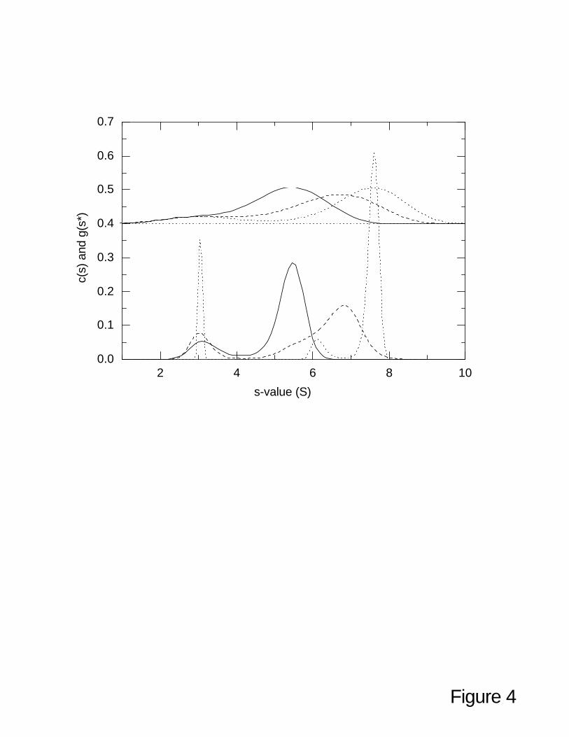
additional resolution can be advantageous. Figure 4 shows c(s) profiles of our simulated model system

in the presence of 20% contamination with a small species that does not participate in the self-

association. This species is visible in the new peak at 3 S. If such a peak can be clearly identified as

contaminating species not participating in the self-association, it can be excluded from the integration

range. The resulting weight-average s-values for the interacting system remained within < 0.5% of the

values obtained in the absence of the contaminating species. Clearly, since the distributions ls-g*(s)

and g(s*) only reflect the shapes of the sedimentation boundary, they do not provide the resolution to

locate the correct integration limits. In contrast, diffusional deconvolution of c(s) can resolve the

contaminating species. Under some conditions for the lowest concentration data, we found that the

peak of the small 3 S species appeared at a slightly higher s-value (data not shown). This reflects a

known property of the maximum entropy regularization that under some conditions, nearby peaks can

‘attract’. This happens only for the lowest concentration because of the very low signal-to-noise ratio

and the corresponding high bias from the regularization. Interestingly, despite this fact, the weight-

average sedimentation coefficient is not affected, which reflects the overruling importance of the

quality of representation of the original sedimentation boundaries (which by design are unchanged by

the regularization, within the predefined confidence level).

A closer look at the isotherms of sw for the different methods plotted against the loading

concentration indicates that the obtained values are slightly lower than the expected isotherm for the

system underlying the simulation (a section of the isotherm is expanded in Figure 5, full circles and

squares). This is consistent with the theory, which predicts radial dilution to lower the sw values. The

21

use of concentration values based on average dilution during the entire sedimentation process (Eq. 8)

provides a small, but effective correction for the radial dilution (open circles). It was found to increase

the precision by ~ 1%, which is significant compared to the precision of up to 0.1% that can be

obtained in sedimentation velocity experiments. For comparison, the differential second moment

method requires the average plateau concentrations at the time of the scans, which are significantly

different from the loading concentrations (Figure 5, open triangles). We confirmed that the latter

method is completely independent of the prior history of the sedimentation process and of the location

of the meniscus position (data not shown). (A disadvantage of this method, however, is that the

baseline signal has to be known.)

Figure 6A illustrates why it is important to have the most precise isotherm values possible:

Shown are the sw(c) data in comparison with isotherms assuming different values for the binding

constant, and the monomer and dimer s-values. It should be noted that the best-fit analysis of the sw(c)

data results in parameters very close to those underlying the simulations (solid line). However, it is

apparent from Figure 6 that isotherms with very different binding constants differ surprisingly little

from the calculated sw(c) data, and that small random or systematic errors in the sw(c) data can

therefore lead to large errors in the calculated binding parameters. This example also illustrates that a

large concentration range is crucial. The model system was designed to simulate approximately the

largest concentration range ordinarily possible without introducing non-ideal sedimentation at high

concentrations. In contrast, Figure 6B shows the isotherm obtained for a weaker monomer-dimer self-

association studied at concentrations including the range where non- ideal sedimentation is highly

relevant. The negative concentration dependence at the higher concentrations broadens the isotherm

and leads to the decrease of sw. These data can be analyzed analogously if the sw(c) isotherms consider

the hydrodynamic s(c) dependence s = s0 /(1+ksc). A moderate correlation of the parameter values for

ks, KA, and s2 was observed. In any case, however, for the analysis of the sw(c) isotherm, it is highly

22

desirable to introduce independent information, for example, on the monomer sedimentation

coefficient, the equilibrium constant, or limits for the monomer and dimer sedimentation coefficients

(or their ratio) derived from hydrodynamic models.

In this regard, the error estimates for the sw(c) data are of great importance. Shown in Figure 6A

are those obtained from DCDT+ for the g(s*) method (solid squares and error bars). They are

determined by the signal- to-noise ratio of the data (which are dependent on the wavelength for the

simulated absorbance experiments (Figure 1)), and also by the maximum number of scans that can be

used in the g(s*) analysis. (It should be noted that the simulated data have a conservative estimate of

0.01 OD for the experimental noise, which is on the order but may slightly exceed that commonly

observed.) In the absence of independent information on the monomer sedimentation coefficient, it

would be highly desirable to incorporate experiments at lower concentration, but the lower signal-to-

noise ratio would result in unacceptably large error bars for the corresponding sw-value. To address the

lack of an error estimate in the software SEDFIT for the sw-values from integration of the ls-g*(s) and

c(s) distributions, the Monte-Carlo simulations in SEDFIT were expanded to allow evaluation of the

statistics of the sw-values. These calculations can be performed relatively fast, since the two most

time-consuming steps in the algebraic formalism of the distribution method are the calculation of the

model- functions for each s-value and the normal matrix (67), which do not change for the Monte-Carlo

iterations. The resulting error estimates for the data shown in Figure 6 were < 0.005 S (including

degrees of freedom for time-invariant noise), and on the average a factor 10 – 40 smaller than those

from g*(s), reflecting the significantly larger data basis in the c(s) analysis. This can be very

significant, in particular, for the low concentration and low signal-to-noise data, and allows extending

the concentration range of the isotherm data. This is indicated as triangles in Figure 6, which show the

sw-values obtained at concentrations as low as 0.025 µM (under conditions equivalent to those

simulated in Figure 1, assuming detection at 230 nm). Despite the small signal-to-noise ratio of only ~

23

2:1 in the lowest concentration data, 40 scans with ~ 40,000 data points can be included in the analysis,

resulting in relatively small statistical errors in the derived sw-values. It was observed, however, that at

signal-to-noise ratios < 5, both maximum entropy and Tikhonov-Phillips regularization of the

distribution introduce a bias in the sw values with a magnitude of the order of the statistical errors. This

systematic error can be easily eliminated by removing the regularization. For data at higher signal-to-

noise ratios, this error is negligible.

As an alternative approach, global direct modeling of the sedimentation boundaries at different

concentrations by solutions of the Lamm equations for fast reversible self-association was explored.

Conceptually, this approach has a drawback in that it requires additional information on the diffusion

coefficients of all species. Also, the basic problem of correlations between the sedimentation

coefficients and the equilibrium constants remains. However, one can use information on known

molar masses of the monomer and oligomers to calculate these diffusion coefficients with the

Svedberg equation (1). Beyond the possibility to identify the self-association scheme (see discussion),

the promise of this approach lies in the shapes of the sedimentation profiles, which report on the

sedimentation over a large concentration range in a single experiment, and the use of the rotor speed as

an additional experimental parameter tha t balances the relative extent of sedimentation and diffusion.

This approach is explored in the following by application to the model system.

First, we compared the Lamm equation fits to the individual sedimentation velocity experiments.

None of the data sets individually contained enough information to identify the correct parameters.

For example, when the monomer sedimentation coefficient s1 was held constant at the wrong value of

2 S while the other parameters s2 and KA were allowed to float, the impostor model produced an

increase in the rms deviation for the 0.2 µM, 2 µM, and 20 µM data sets individually by only 2%.

However, when taken together in a global analysis, an average increase of ~ 30% was observed, with

clearly systematic residuals. This illustrates the advantage of global analysis. Sometimes, it was

24

difficult to converge to the global best- fit, because the data at high concentration with their relatively

steep gradients can initially dominate the optimization process and cause the parameters to fall into a

local minimum. Therefore, we found it frequently advantageous to adhere to the following sequence:

First, a local fit was performed to each data set, and the local concentration parameters were fixed.

Then, the low concentration data were modeled, using estimates for s1, s2, and KA (derived from local

analyses or sw isotherms), and the monomer s-value was fixed. Next, a sequence of global fits was

performed with floating s2 and KA, floating s1, s2, and KA, and finally with floating local concentrations,

s1, s2, and KA.

For comparison of the global fits to different combinations of experimental concentrations, Tables

1 and 2 list the error estimates derived from Monte-Carlo analysis, with and without treating the

monomer molar mass as an unknown, respectively. Several tendencies are apparent: For the

sedimentation coefficients, obviously conditions must be established to populate the dimer in order to

determine s2. Generally, data at higher concentration have more information, which is a consequence

of these experiments spanning a broader concentration range. Global analysis of data at different

concentrations is crucial for high precision in the association constant and the monomer s-value.

However, including more intermediate concentrations does not result in a very significant gain, which

is again a consequence of each experiment already spanning a large concentration range due to the

dilution in the sedimentation boundary (i.e., due to the boundary shape information). Lower rotor

speeds are in some cases slightly better for determining the binding constant, but significantly worse

for the measurement of the sedimentation coefficients. The combination of data from different rotor

speeds can be beneficial, but the gains are not very substantial. For the most parsimonious

experimental design, it appears that a very high and a very low concentration at a high rotor speed are

best (Table 1). Under these conditions, the monomer molar mass can be estimated from the

sedimentation data, without significant loss of precision in the other parameters (Table 2).

25

Obviously, much better precision is obtained if prior knowledge is available (Table 1). For

example, independent information on the sedimentation coefficients may be obtained sometimes

through site-directed mutagenesis, binding of small ligands that stabilize or destabilize the oligomeric

states, or by applying different solvent conditions that affect the thermodynamics or the kinetics of the

self-association equilibrium (24, 29, 30, 33, 84, 85). Further information may be derived from

hydrodynamic modeling of the monomer and oligomer, either through simple geometric models or

utilizing a crystal structure (86, 87). Remarkably, the most precise determination of the binding

constant was obtained in single experiments at moderate and high concentrations when the monomer

and dimer s-value were known (Table 1). Vice versa, significantly higher precision in the

sedimentation coefficients is possible if the equilibrium constant is known. Prior knowledge on the

association constants may be available from sedimentation equilibrium experiments (such as shown in

Figure 7 for our model system). In this case, however, from a statistical perspective, the global

analysis of sedimentation velocity and sedimentation equilibrium is much more straightforward

approach. The SEDPHAT software is designed to incorporate both thermodynamic and hydrodynamic

data into a global model. As compared to the separate model, such a global approach can improve the

precision of both the equilibrium constant and the sedimentation coefficients (Table 1 and 2).

Combination of velocity and equilibrium data is particularly useful when the molar mass is unknown

(Table 2).

Interestingly, the detection of fractions of material incompetent to participate in the reversible

equilibrium, such as incompetent monomer, or irreversibly aggregated dimer, can be very

straightforward by global modeling of the sedimentation boundaries (Table 1). As illustrated in Figure

8, incompetent monomer results in a clearly formed additional sedimentation boundary in the high

concentration data, while incompetent dimer would form a clearly visible additional fast sedimentation

boundary in the low concentration data (data not shown). Therefore, the detection of the incompetent

26

fractions does interfere with the analysis of the associating system. Although detection of incompetent

populations is also possible by sedimentation equilibrium analysis (88), the separation of species in

sedimentation velocity combined with direct modeling of the boundaries provides a unique tool to

detect and consider incompetent species. In principle, other contaminating species can be taken into

consideration similarly, by modeling as a superposition with an additional, noninteracting component.

It has been long known that the shape of the sedimentation boundaries has information on the

nature of the association scheme (21, 89, 90). To illustrate this property, Figure 9 shows a comparison

of sedimentation profiles for stable dimer, monomer-dimer, monomer-trimer, monomer-tetramer, and

monomer-dimer-tetramer self-association (Figure 9). In all cases, the concentration was assumed to be

five-fold above the characteristic equilibrium dissociation constants. It is apparent that with increasing

association order (1-2, 1-3, to 1-4) the boundary assumes an increasingly bimodal shape, with a steeper

leading and a longer trailing component. This boundary shape can also be qualitatively diagnosed a

transformation of a data subset, such as g(s*) or ls-g*(s). For quantitative analysis in the context of

direct modeling of the sedimentation profiles, we have studied how well the association schemes can

be distinguished given unknown sedimentation coefficients, binding constants, and noisy experimental

data. For example, the monomer-dimer data shown in Figure 9B (at 10 µM, with 0.01 OD random

noise added) can be modeled by the monomer-trimer scheme (such as Figure 9C) with a best- fit

reduced χ2 of ~ 14 % above the expected value (or ~ 7 % if the monomer molar mass was allowed to

float to 68 kDa). This may not be enough, in practice, to unambiguously identify the scheme. In a

global analysis of data at 0.2, 2 and 20 µM, the best- fit results in an increase of the reduced χ2 of ~ 43

% (log10(KA13) = 11.0 and s1 = 5.5 S, and s3 = 7.9 S) but only 12 % if the monomer mass in treated as

an unknown (converging to 71 kDa, with log10(KA13) = 11.2 and s1 = 5.5 S, and s3 = 7.8 S). Slightly

larger deviations are found if data at different rotor speeds are incorporated in the global fit. Thus,

global modeling of the sedimentation profiles can be very helpful for the determination of the

27

association scheme, in particular if the molar mass of the monomer is known. Beyond the χ2 of the fit,

the returned parameter values for the sedimentation coefficients are closer together in the impostor

model, suggesting an implausible hydrodynamic shape of the trimer compared to the monomer.

Hydrodynamic non- ideality can also be taken into account in the global model. Finite element

solutions of the Lamm equation with both self-association and hydrodynamic repulsive non- ideality

can be obtained in the formalism of locally concentration dependent sedimentation coefficients (38, 41,

77). The negative concentration-dependence of the sedimentation coefficient at higher concentrations

results in a characteristic steepening and reduction of the diffusional spread of the sedimentation

boundaries (91), which is distinct from the boundary shapes caused by of self-association. This

provides sufficient information to determine the non- ideality coefficient ks with good precision as an

additional parameter in the global model (data not shown).

Discussion

In the present paper, we have proposed several new tools for analyzing protein self-association by

sedimentation velocity. There are two general approaches: the traditional calculation of weight-

average sedimentation coefficients as a function of chemical composition followed by a separate

isotherm analysis, and the direct modeling of the sedimentation profile from multiple experiments in a

global analysis. Both can be combined with other available prior knowledge, including binding

constants or s-values of the interacting species, derived from ultracentrifugation experiments with

protein variants, or under modified conditions, or from hydrodynamic consideration of simple

geometric association models and/or a crystal structure (86, 87). However, the approaches for

sedimentation analysis differ in their practical requirements for sample purity and experimental

conditions. The former approach is valid for any association model, including hetero-associations, but

the latter requires a specific association model.

28

First, based on the theoretical foundation of the second moment definition of a weight-average

sedimentation coefficient sw, we have shown that integration of any of the currently used differential

sedimentation coefficient distributions g(s*), ls-g*(s), and c(s) can lead to a well-defined isotherm

sw(c), which can be used to characterize the thermodynamics of the protein interaction. While the

g(s*) distribution has long been used for this purpose, the present analysis showed for the first time

that also the newer approaches, in particular c(s), which use regularization and diffusional

deconvolution techniques, are fully consistent with the rigorous definition of sw. Their utility and

advantages in comparison with other approaches will be discussed below.

An important condition is for calculating well-defined sw-values is that the sedimentation

boundaries are faithfully described by the distribution. Although this condition may seem trivial, it

raises several interesting points. With regard to the g(s*) distribution, since it is based on a data

transformation (64), the quality of its representation of the original sedimentation profiles cannot be

easily assessed. It is well-known that the numerical approximation of dc/dt (64), which is a central

computational step in this approach for eliminating time-invariant (TI) noise components of the raw

data (see below), can produce distortions and artificial broadening in the g(s*) distribution (65). In a

rectangular cell approximation, this effect has been described as convolution of g(s*) with a hyperbola

segment (66). Semi-empirical rules have been published (65) for the selection of a suitable data subset

that avoids artificial broadening of the g(s*) distribution. However, because the g(s*) distribution is

based on a data transformation, the question how artificial broadening relates to the original data has

not been asked. In the present paper, we have introduced a back-transformation of g(s*) into the

original data space. Since g(s*) is computed for a discrete set of s-values, one can reconstruct the

corresponding sedimentation boundaries as a superposition of a large number of step-functions (66).

The degrees of freedom that were eliminated in the forward-transform by the differentiation dc/dt can

be restored by algebraically calculating the best- fit TI noise components (52), which are

29

unambiguously determined for any model of the sedimentation profiles (68). (This step makes the

additional assumption that the TI noise is truly constant, but after extensive application of systematic

noise decomposition, little evidence for such instability is usually found.) As a result, the back-

transform can be used to verify quantitatively how well the original sedimentation data are represented

by the g(s*) distribution. In this way the g(s*) approach can be changed from a ‘data transform’ into a

model for the sedimentation profiles that produces residuals of the fit, which can be compared with

other sedimentation models, thereby closing a gap in the relationship between the different approaches

for interpreting sedimentation velocity data. As shown in Figure 3, a g(s*) analysis using a high

number of scans that led to artificial distortion of g(s*) modeled the data very poorly, while the data

were well-described when not exceeding recommended number of scans. This shows that the rms

error of the back-transform could be used as a criterion for the selection of the appropriate data subset.

Interestingly, when applied to the analysis of experimental interference optical sedimentation profiles,

we observed that the back-transform of g(s*) calculated by DCDT+ under recommended conditions

produced estimates of the TI noise that were virtually identical to those from other direct sedimentation

models (data not shown). In the present context, the faithful representation of the original

sedimentation boundaries is critical for determining thermodynamically well-defined weight-average

sedimentation coefficients.

The sedimentation coefficient distributions ls-g*(s) and c(s) are already direct models of the

sedimentation profiles, utilizing the recently introduced method for including the time- invariant and

radial- invariant noise components of the sedimentation data into the model (52). The question of

representation of the sedimentation profiles is therefore more straightforward. For the apparent

sedimentation coefficient distribution ls-g*(s), the limiting factor is that diffusion is not taken into

account. For example with the data shown in Figure 3, the ls-g*(s) distribution can provide a

reasonably good sedimentation model (rms error 0.016) over the complete range shown, but the quality

30

of fit will decrease if more scans are included (data not shown). Because boundary broadening by

diffusion is taken into account in the c(s) method, there is no limit apparent, and the complete set of

experimental scans can be modeled well and included in the analysis. Clearly, a larger number of

scans translates into more precise estimates for sw.

Both the ls-g*(s) and the c(s) methods utilize regularization, which apply Bayesian principles to

favor distributions that are more consistent with our prior expectation of smoothness or high

informational entropy. This can have a significant influence on the shape of the calculated

distribution, and it is an important question how this will influence the calculated weight-average

sedimentation coefficients. To estimate this influence, the sole criterion is, again, the quality of the

sedimentation model. Since the parsimony prior of the regularization is scaled such that it does not

decrease the quality of fit by more than a predefined confidence level (usually one standard deviation),

the errors translated in the weight-average sedimentation coefficients cannot exceed the statistical

limits. Accordingly, from the analysis of our model data, we found the bias from the regularization to

affect the sw-values only within a magnitude equal or smaller than the statistical errors from the noise

in the sedimentation data. As a consequence, regularization is of concern and should be switched off

only when determining sw-values from data with extremely low signal-to-noise ratio (e.g., smaller than

five).

Because the analysis of the sw-isotherm can be very ill-conditioned (Figure 6), the ability to cover

a large concentration range and the precision of the sw-values is very important. In the present paper,

we have implemented Monte-Carlo simulations in order to calculate error estimates for the sw-values

from integration of c(s). As shown in Figure 6, the errors are significantly smaller than those estimated

for the g(s*) method, largely probably due to the several times larger data sets that can be included in

c(s). Noise amplification in the g(s*) method in the pairwise subtraction of scans may also be a factor.

With c(s) loading concentrations that produce signals as small as two or three times the noise can be

31

easily analyzed. This is of significance in particular for the data at lower concentrations, where the

signal-to-noise ratio is relatively low, but where the isotherm would contain very significant

information on the s-value of the smallest species (Figure 6).

Another interesting feature when using the c(s) distribution for determining sw-values is the

deconvolution of diffusional broadening. As has been pointed out before (67, 68), the deconvolution is

based on the assumption of noninteracting species, and for interactions that are reversible on the time-

scale of the sedimentation experiment, the peaks in the c(s) distribution do not correspond to the s-

values of sedimenting species. This is illustrated in Figure 2, which also suggests that even for

concentrations 10fold lower and higher than KD one can only very cautiously interpret the c(s) curves,

for example, to extrapolate starting values for the monomer and oligomer s-values for the isotherm

analysis. (This is in contrast to slowly re-equilibrating systems, where the peaks of the c(s) curves do

reflect the oligomeric species present (54, 73).) In any case, the diffusional deconvolution can be

utilized for the detection of species and contaminants that do not participate in the association,

provided they sediment at rates outside the range of s-values of the associating protein and its

complexes. This is shown in Figure 4, where the superposition of c(s) distributions at different

concentrations reveals a constant and separate 3 S species, which can be excluded from the integration

range of sw.

A general concern when using the c(s) distribution is that it is based on an approximation for the

frictional ratios f/f0 of noninteracting sedimenting components, and the assumption that these can be

sufficiently well approximated by a weight-average (f/f0)w. In contrast, no such approximation appears

necessary in the analysis with the g(s*) or ls-g*(s) method. However, both g(s*) and ls-g*(s) are

apparent sedimentation coefficient distributions of hypothetical non-diffusing (and noninteracting)

particles, which is equivalent to the limit of infinite frictional ratios for all species (68). Although the

estimate of a weight-average (f/f0)w in the c(s) method may not be precise for all species, f/f0 is not a

32

very shape-sensitive parameter and it has been shown that the peak positions of c(s) are largely

insensitive to the value of (f/f0)w (68). Allowing for diffusion of the species with finite f/f0 values is

more realistic and provides a better model of the sedimentation profiles, and permits extending the data

set to be modeled from a small data subset in g(s*) and ls-g*(s) to the complete sedimentation process,

thereby both increasing the resolution of the distribution and the precision of the sw values. As shown

in the theory section, the only requirement for a precise sw value is a good model of the sedimentation

profiles, which can usually be assured by the optimization of (f/f0)w through non-linear regression of

the experimental data. To this extent, the assumption of (f/f0)w is not critical for the determination of

sw. On the other hand, if a good fit cannot be achieved, for example when analyzing strongly

concentration-dependent non- ideal sedimentation with repulsive interactions, the restriction of the data

subset and/or the use of the apparent sedimentation coefficient distributions g(s*) and ls-g*(s) which

represent only the overall boundary shape appears advantageous.

A second important element for generating isotherm data sw(c), after determining precise sw-values

with any method, is the assignment of the correct concentration values. It is well-known that the

sedimentation process slows down due to significant radial dilution (1), and that for reversibly

interacting systems, the loading concentration is not the correct concentration. The theoretical analysis

shows that, perhaps contrary to common expectation, the plateau concentration is not correct either, if

the distribution is derived from any of the established differential sedimentation coefficient

distributions. The reason is that the sedimentation coefficient distributions are based on equations that

integrate the entire sedimentation process, from the start of the centrifuge to the measurement of the

boundary position. Therefore, the time-average of the radial dilution that the boundary has

experienced during the whole process has to be taken into consideration. The proposed correction

factors amount to as much as 10 % in concentration, or ~ 1 % in the s-values. This may seem a small

factor, but it is significantly larger than the experimental error in s, and can be relevant considering the

33

difficulties of the subsequent analysis of the isotherm (Figure 5 and 6).

We have also implemented a differential second moment method (Eq. 3) which does not imply

any prior history. In this form, the relevant concentrations are the plateau concentrations (averaged

only between the scans used in the analysis). This approach has the practical advantage that it can be

applied to data from experiments with initial convection or temperature instability, or where the

meniscus cannot be located, as long as the sedimentation profiles considered for analysis reflect free

sedimentation. It shares these properties with the technique of using an experimental scan to initialize

a Lamm equation model (40), but the derived sw values from the differential second moment method

are more general and applicable to any reactive or non-reactive multi-component system.

In summary, the above methods allow the determination of precise weight-average sedimentation

coefficients and effective concentrations to form the isotherm sw(c). In our experience, the diffusion

deconvoluted sedimentation coefficient distribution c(s) usually gave the best results. The sw(c) can

then be subjected to a separate thermodynamic analysis with a model for the interaction, with binding

constants and usually with monomer and oligomer sedimentation coefficients as unknowns.

A second major family of methods is the direct modeling of the sedimentation profiles with

numerical solutions of the Lamm equation for fast reversible self-association. Global modeling of

different sedimentation velocity experiments is not new; it has been applied, for example, to the study

of non- ideal sedimentation in complex solvents (77), or for the characterization of multiple

independent species of a viral protein (73), and it is also related to the global modeling of time-

difference data for heterogeneous interactions (49). However, while increasing computational power

makes it possible to readily apply this tool, so far no analysis of the properties and optimal

experimental conditions for the application of global direct sedimentation modeling has been

published. In the present paper, we have introduced a new software platform, SEDPHAT, for the

global analysis of hydrodynamic and thermodynamic data from sedimentation velocity, sedimentation

34

equilibrium, and dynamic light scattering experiments. Although not discussed here, it permits very

flexible characterization of noninteracting species. The main goal in the present context was to

provide a comprehensive analysis of the potential for analyzing protein self-association.

A central aspect of this approach is that the sedimentation profiles contain information on the

complete isotherm up to the loading concentration. In addition, as many data points can be included as

in the c(s) analysis discussed above. For example, in our simulated model data that mimics the signal-

to-noise ratio typically achieved with the absorption optics, a single experiment at approximately 5fold

KD gives surprisingly good precision in the derived parameters. Significant improvement can be

achieved already with the combination of an experiment at very low and very high loading

concentrations (Table 1). Clearly, much fewer concentrations are required to determine the binding

constant and the s-values of the monomer and oligomers than with the analysis of an sw- isotherm.

Also, the monomer molar mass can be readily determined in this approach. It should be noted that the

presented global Lamm equation model requires that the reaction kinetics is fast compared to the

sedimentation. This may be known from other techniques, or may be studied from the concentration

and rotor speed dependence of the peak positions of c(s).

Global direct modeling of the sedimentation profiles has several other remarkable properties. It

has been long known that the boundary shape is specific for the different association schemes. For

example, Gilbert has predicted by theoretical considerations in the absence of diffusion that the

sedimentation boundaries exhibit increasing asymmetry and higher steepness of the leading edge for

higher order associations (21, 89). This clearly distinguishes rapid from slow self-association

equilibria ((54) and Figure 9). Similar boundary distortions with stronger boundary deceleration

appear in analytical zone centrifugation (92, 93) (data not shown). So far, the reverse problem has not

been examined, if the association scheme can be uniquely identified with direct modeling the

sedimentation profiles given noisy experimental data. When examining the quality of the fit of our

35

simulated monomer-dimer system with an imposter monomer-trimer model, we found that a single

sedimentation experiment may not contain enough data to unambiguously distinguish the two. With

global modeling of several experiments at different concentrations, however, the association scheme

was much better determined. A practical application of this is the multi-step self-association of gp57A

of the bacteriophage T4, which was analyzed by sedimentation velocity and other biophysical methods

(59). In these studies, global modeling of the sedimentation boundaries provided the most convincing

evidence for the determination of the association scheme.

Another advantage is the ability to identify incompetent species. Because monomers or oligomers

that do not participate in the association separate as independent species and can form a separate

boundary, their consideration does not significantly influence the characterization of the association.

This may be highly useful, for example, where stable covalently linked oligomers can occur in addition

to the reversible ones (94), or where some of the protein may be partially unfolded and incompetent to

associate (88, 95). It is possible to identify the contamination with incompetent species also by

sedimentation equilibrium (88) (for example in an apparent concentration dependence of the estimate

of the association constant). However, because the competent and incompetent species of the same

oligomer do contribute to the sedimentation equilibrium signal in the same way, they can be

distinguished only after analysis of a large experimental data basis. In comparison, their

hydrodynamic separation in sedimentation velocity can be even qualitatively apparent in a single

experiment.

Finally, an important feature of the global direct modeling of the sedimentation profiles is that it

can be extended to a global analysis of sedimentation equilibrium and velocity data. This can be

useful, in particular, to combine partial information from either approach. An open problem when

combining data sets from different techniques is their relative weight. One could argue that a purely

statistical weighting according to statistical noise of the data points is not optimal, since it does not

36

take into account the different robustness of the experiments against imperfections leading to

systematic errors. A limitation of the global analysis of experiments at different rotor speeds is a

possible pressure effect, which in some cases may lead to inconsistent binding constants for the

different experiments. Partial-volume changes of proteins upon oligomerization have been observed

occasionally at pressures accessible to the analytical ultracentrifuge (96, 97), but are usually visible at

higher pressures (2).

In summary, we have further explored known approaches and developed several new tools for two

different general strategies for the analysis of protein self-association by sedimentation velocity. The

route via the concentration dependence of the weight-average sedimentation coefficients followed by

isotherm analysis has the advantage that any impurities or aggregates that are not part of the interacting

system can be excluded from the analysis, if they can be hydrodynamically separated. The diffusion

deconvoluted sedimentation coefficient distribution c(s) is particularly well suited for this approach, as

it allows the widest concentration range and has the highest precision among the sedimentation

coefficient distributions. Conversely, the strategy of global modeling of the sedimentation profiles

allows utilizing the largest data sets, requires fewer experiments, and permits the identification of the

association scheme, because the information from the shape of the sedimentation profiles is fully

exploited. However, consideration of all sedimenting species is necessary, which makes this method

currently only practical with highly pure samples. In the future, it may be possible to partially

eliminate this drawback by a hybrid approach, combining a sedimentation model for a specific solution

component with a continuous sedimentation coefficient distribution describing species sedimenting at

different rates.

Acknowledgment

I thank Drs. Allen Minton and Jacob Lebowitz for their discussions and critical reading of the

manuscript.

37

References

1. Svedberg, T., and Pedersen, K. O. (1940) The ultracentrifuge, Oxford University Press, London.

2. Schachman, H. K. (1959) Ultracentrifugation in Biochemistry, Academic Press, New York.

3. Rivas, G., Stafford, W., and Minton, A. P. (1999) Characterization of heterologous protein-protein interactions via analytical ultracentrifugation. Methods: A Companion to Methods in Enzymology 19, 194-212.

4. Liu, J., and Shire, S. J. (1999) Analytical ultracentrifugation in the pharmaceutical industry. J Pharm Sci 88, 1237-41.

5. Arisaka, F. (1999) Applications and future perspectives of analytical ultracentrifugation. Tanpakushitsu Kakusan Koso 44, 82-91.

6. Laue, T. M., and Stafford, W. F. I. (1999) Modern applications of analytical ultracentrifugation. Annu. Rev. Biophys. Biomol. Struct. 28, 75-100.

7. Schuck, P., and Braswell, E. H. (2000) in Current Protocols in Immunology (Coligan, J. E., Kruisbeek, A. M., Margulies, D. H., Shevach, E. M., and Strober, W., Eds.), pp. 18.8.1-18.8.22, John Wiley & Sons, New York.

8. Lebowitz, J., Lewis, M. S., and Schuck, P. (2002) Modern analytical ultracentrifugation in protein science: a tutorial review. Protein Sci 11, 2067-79.

9. Schachman, H. K. (1992) in Analytical Ultracentrifugation in Biochemistry and Polymer Science (Harding, S. E., Rowe, A. J., and Horton, J. C., Eds.), pp. 3-15, Royal Society of Chemistry, Cambridge.

10. Schuster, T. M., and Toedt, J. M. (1996) New revolutions in the evolution of analytical ultracentrifugation. Curr Opin Struct Biol 6, 650-8.

11. Hensley, P. (1996) Defining the structure and stability of macromolecular assemblies in solution: the re-emergence of analytical ultracentrifugation as a practical tool. Structure 4, 367-73.

12. Stafford, W. F. (1997) Sedimentation velocity spins a new weave for an old fabric. Curr. Opin. Biotechnology 8, 14-24.

13. Schwert, G. w. (1949) The molecular size and shape of the pacreatic proteases. Sedimentation studies on chymotrypsinogen and on alpha- and gamma-chymotrypsin. J Biol Chem 179, 655-664.

14. Massey, V., Harrington, W. F., and Hartley, B. S. (1955) Certain physical properties of chymotrypsin and chymotrypsinogen using the depolarization of fluorescence technique. Disc. Faraday Soc. 20, 24-32.

15. Oncley, J. L., Ellenbogen, E., Gitlin, D., and Gurt, F. R. N. (1952) Protein-protein interactions. J Phys Chem 56, 85-92.

16. von Hippel, P. H., and Waugh, D. F. (1955) Casein: Monomers and polymers. J. Am. Chem. Soc. 77, 4311-4319.

17. Field, E. O., and Ogston, A. G. (1955) Boundary spreading in the migration of a solute in rapid dissociation equilibrium. Theory and its application to the case of human hemoglobin. Biochem. J. 60, 661-665.

18. Tiselius, A. (1930) The moving-boundary method of studying the electrophoresis of proteins. Nova Acta Regia Societatis Scientiarum Upsaliensis. Series IV. 7, 1.

38

19. Baldwin, R. L. (1953) Sedimentation coefficients of small molecules: Methods of measurement based on teh refractive- index gradient curve. The sedimentation coefficient of polyglucose A. Biochem. J. 55, 644-648.

20. Steiner, R. F. (1954) Reversible association processes of globular proteins. V. The study of associating systems by the methods of macromolecular physics. Arch. Biochem. Biophys. 49, 400-416.

21. Gilbert, G. A. (1955) Disc. Faraday Soc. 20, 68-71.

22. Rao, M. S. N., and Kegeles, G. (1958) An ultracentrifuge study of the polymerization of alpha-chymotrypsin. J. Am. Chem. Soc. 80, 5724-5729.

23. Timasheff, S. N., and Townend, R. (1961) Molecular interactions in beta- lactoglobulin. V. The association of the genetic species of beta- lactoglobulin below the isoelectric point. J. Am. Chem. Soc. 83, 464-469.

24. Frigon, R. P., and Timasheff, S. N. (1975) Magnesium-induced self-association of calf brain tubulin. II. Thermodynamics. Biochemistry 14, 4567-4573.

25. Frigon, R. P., and Timasheff, S. N. (1975) Magnesium-induced self-association of calf brain tubulin. I. Stoichiometry. Biochemistry 14, 4559-4566.

26. Cann, J. R. (1978) Measurements of protein interactions mediated by small molecules using sedimentation velocity. Methods Enzymol 48, 242-248.

27. Hesterberg, L. K., and Lee, J. C. (1981) Self-association of rabbit muscle phosphofructokinase at pH 7.0: stoichiometry. Biochemistry 20, 2979-2980.

28. Harris, S. J., Williams, R. C., and Lee, J. C. (1995) Self-association of escherichia coli DNA-dependent RNA polymerase core enzyme. Biochemistry 34, 8752-8762.

29. Cole, J. L. (1996) Characterization of human cytomegalovirus protease dimerization by analytical ultracentrifugation. Biochemistry 35, 15601-15610.

30. Lowman, H. B., Fairbrother, W. J., Slagle, P. H., Kabakoff, R., Liu, J., Shire, S., and Hébert, C. A. (1997) Monomeric variants of IL-8: Effects of side chain substitutions and solution conditions upon dimer formation. Protein Science 6, 598-608.

31. Lorbert, S., Ingram, J. W., Hill, B. T., and Correia, J. J. (1998) A comparison of thermodynamic parameters for vinorelbine- and vinflunin- induced tubulin self-association by sedimentation velocity. Mol. Pharmacol. 53, 908-915.

32. Correia, J. J., Chacko, B. M., Lam, S. S., and Lin, K. (2001) Sedimentation studies reveal a direct role of phosphorylation in Smad3:Smad4 homo- and hetero-trimerization. Biochemistry 40, 1473-82.

33. Buisson, M., Valette, E., Hernandez, J. F., Baudin, F., Ebel, C., Morand, P., Seigneurin, J. M., Arlaud, G. J., and Ruigrok, R. W. (2001) Functional determinants of the Epstein-Barr virus protease. J Mol Biol 311, 217-28.

34. Correia, J. J. (2000) Analysis of weight average sedimentation velocity data. Methods in Enzymology 321, 81-100.

35. Fujita, H. (1975) Foundations of ultracentrifugal analysis, John Wiley & Sons, New York.

36. Lamm, O. (1929) Die Differentialgleichung der Ultrazentrifugierung. Ark. Mat. Astr. Fys. 21B(2), 1-4.

37. Bethune, J. L., and Kegeles, G. (1961) Countercurrent distribution of chemically reacting systems. III. Analogs of moving boundary electrophoresis and sedimentation. J. Phys. Chem. 65, 1761-1764.

39

38. Cox, D. J. (1969) Computer simulation of sedimentation in the ultracentrifuge. IV. Velocity sedimentation of self-associating solutes. Arch. Biochem. Biophys. 129, 106-123.

39. Claverie, J.-M. (1976) Sedimentation of generalized systems of interacting particles. III. Concentration-dependent sedimentation and extension to other transport methods. Biopolymers 15, 843-857.

40. Schuck, P., MacPhee, C. E., and Howlett, G. J. (1998) Determination of sedimentation coefficients for small peptides. Biophys. J. 74, 466-474.

41. Schuck, P. (1998) Sedimentation analysis of noninteracting and self-associating solutes using numerical solutions to the Lamm equation. Biophys. J. 75, 1503-1512.

42. Schuck, P. (2003) A model for sedimentation in inhomogeneous media. II. Compressibility of aqueous and organic solvens. Biophys. Chem. in press.

43. Cann, J. R., and Oates, D. C. (1973) Theory of electrophoresis and sedimentation for some kinetically controlled interactions. Biochemistry 12, 1112-1119.

44. Cann, J. R. (1978) Kinetically controlled mass transport of associating-dissociating macromolecules. Methods Enzymol 48, 248-270.

45. Cann, J. R. (1994) in Modern Analytical Ultracentrifugation (Schuster, T. M., and Laue, T. M., Eds.), pp. 171-188, Birkhauser, Boston.

46. Stafford, W. F. (1994) in Modern Analytical Ultracentrifugation (Schuster, T. M., and Laue, T. M., Eds.), pp. 119-137, Birkhauser, Boston.

47. Philo, J. S. (1997) An improved function for fitting sedimentation velocity data for low molecular weight solutes. Biophys. J. 72, 435-444.

48. Behlke, J., and Ristau, O. (1997) Molecular mass determination by sedimentation velocity experiments and direct fitting of the concentration profiles. Biophys. J. 72, 428-434.

49. Stafford, W. F. (1998) Time difference sedimentation velocity analysis of rapidly reversible interacting systems: Determination of equilibrium constants by global non- linear curve fitting procedures. Biophys. J. 74(2), A301.

50. Schuck, P., and Millar, D. B. (1998) Rapid determination of molar mass in modified Archibald experiments using direct fitting of the Lamm equation. Anal. Biochem. 259, 48-53.

51. Demeler, B., Behlke, J., and Ristau, O. (2000) Determination of molecular parameters from sedimentation velocity experiments: Whole boundary fitting using approximate and numerical solutions of the Lamm equation. Methods in Enzymology 321, 36-66.

52. Schuck, P., and Demeler, B. (1999) Direct sedimentation analysis of interference optical data in analytical ultracentrifugation. Biophys. J. 76, 2288-2296.

53. Kar, S. R., Kinsbury, J. S., Lewis, M. S., Laue, T. M., and Schuck, P. (2000) Analysis of transport experiment using pseudo-absorbance data. Anal. Biochem. 285, 135-142.

54. Perugini, M. A., Schuck, P., and Howlett, G. J. (2000) Self-association of human apolipoprotein E3 and E4 in the presence and absence of phopholipid. Journal of Biological Chemistry 275, 36758-36765.

55. Tarabykina, S., Scott, D. J., Herzyk, P., Hill, T. J., Tame, J. R., Kriajevska, M., Lafitte, D., Derrick, P. J., Dodson, G. G., Maitland, N. J., Lukanidin, E. M., and Bronstein, I. B. (2001) The dimerization interface of the metastasis-associated protein S100A4 (Mts1): in vivo and in vitro studies. J Biol Chem 276, 24212-22.

40

56. Strauss, H., Misselwitz, R., Labudde, D., Nicklisch, S., and Baier, K. (2002) NblA from Anabaena sp. PCC 7120 is a mostly alpha-helical protein undergoing reversible trimerization in solution. Eur J Biochem 269, 4617-24.

57. Lewis, R. J., Scott, D. J., Brannigan, J. A., Ladds, J. C., Cervin, M. A., Spiegelman, G. B., Hoggett, J. G., Barak, I., and Wilkinson, A. J. (2002) Dimer formation and transcription activation in the sporulation response regulator Spo0A. J Mol Biol 316, 235-45.

58. Sontag, C. A., Stafford, W. F., and Correia, J. J. (2003) A comparison of weight average and direct boundary fitting of sedimentation velocity data for indefinite polymerizing systems. Biophys Chem in press.

59. Ali, S. A., Iwabuchi, N., Matsui, T., Hirota, K., Kidokoro, S., Arai, M., Kuwajima, K., Schuck, P., and Arisaka, F. (submitted) Rapid and dynamic association equilibrium of a molecular chaperone, gp57A, of bacteriophage T4.

60. Correia, J. J., and Yphantis, D. A. (1992) in Analytical ultracentrifugation in biochemistry and polymer science (Harding, S. E., Rowe, A. J., and Horton, J. C., Eds.), pp. 231-252, The Royal Society of Chemistry, Cambridge, U.K.

61. Schuck, P. (1994) Simultaneous radial and wavelength analysis with the Optima XL-A analytical ultracentrifuge. Progr. Colloid. Polym. Sci. 94, 1-13.

62. Minton, A. P. (1997) Alternative strategies for the characterization of associations in multicomponent solutions via measurement of sedimentation equilibrium. Progr. Colloid Polym. Sci. 107, 11-19.

63. Philo, J. S. (2000) Sedimentation equilibrium analysis of mixed associations using numerical constraints to impose mass or signal conservation. Methods in Enzymology 321, 100-20.

64. Stafford, W. F. (1992) Boundary analysis in sedimentation transport experiments: a procedure for obtaining sedimentation coefficient distributions using the time derivative of the concentration profile. Anal. Biochem. 203, 295-301.

65. Philo, J. S. (2000) A method for directly fitting the time derivative of sedimentation velocity data and an alternative algorithm for calculating sedimentation coefficient distribution functions. Anal. Biochem. 279, 151-163.

66. Schuck, P., and Rossmanith, P. (2000) Determination of the sedimentation coefficient distribution by least-squares boundary modeling. Biopolymers 54, 328-341.

67. Schuck, P. (2000) Size distribution analysis of macromolecules by sedimentation velocity ultracentrifugation and Lamm equation modeling. Biophys. J. 78, 1606-1619.

68. Schuck, P., Perugini, M. A., Gonzales, N. R., Howlett, G. J., and Schubert, D. (2002) Size-distribution analysis of proteins by analytical ultracentrifugation: strategies and application to model systems. Biophys J 82, 1096-1111.

69. Dam, J., and Schuck, P. Calculating sedimentation coefficient distributions by direct modeling of sedimentation velocity profiles. Methods Enzymol in press.

70. Barbier, P., Gregoire, C., Devred, F., Sarrazin, M., and Peyrot, V. (2001) In vitro effect of cryptophycin 52 on microtubule assembly and tubulin: molecular modeling of the mechanism of action of a new antimitotic drug. Biochemistry 40, 13510-9.

71. Hatters, D. M., Lindner, R. A., Carver, J. A., and Howlett, G. J. (2001) The molecular chaperone, α-crystallin, inhibits amyloid formation by apolipoprotein C-II. J.Biol.Chem 276, 24212-24222.

41

72. MacRaild, C. A., Hatters, D. M., Lawrence, L. J., and Howlett, G. J. (2003) Sedimentation velocity analysis of flexible macromolecules: self-association and tangling of amyloid fibrils. Biophys J 84, 2562-9.

73. Taraporewala, Z. F., Schuck, P., Ramig, R. F., Silvestri, L., and Patton, J. T. (2002) Analysis of a temperature-sensitive mutant rotavirus indicates that NSP2 octamers are the functional form of the protein. J Virol 76, 7082-93.

74. Hatters, D. M., Wilson, L., Atcliffe, B. W., Mulhern, T. D., Guzzo-Pernell, N., and Howlett, G. J. (2001) Sedimentation analysis of novel DNA structures formed by homo-oligonucleotides. Biophys. J. 81, 371-381.

75. van Holde, K. E., and Weischet, W. O. (1978) Boundary analysis of sedimentation velocity experiments with monodisperse and paucidisperse solutes. Biopolymers 17, 1387-1403.

76. Claverie, J.-M., Dreux, H., and Cohen, R. (1975) Sedimentation of generalized systems of interacting particles. I. Solution of systems of complete Lamm equations. Biopolymers 14, 1685-1700.

77. Solovyova, A., Schuck, P., Costenaro, L., and Ebel, C. (2001) Non-ideality by sedimentation velocity of halophilic malate dehydrogenase in complex solvents. Biophysical Journal 81, 1868-80.

78. Laue, T. M., Shah, B. D., Ridgeway, T. M., and Pelletier, S. L. (1992) in Analytical Ultracentrifugation in Biochemistry and Polymer Science (Harding, S. E., Rowe, A. J., and Horton, J. C., Eds.), pp. 90-125, The Royal Society of Chemistry, Cambridge.

79. Bevington, P. R., and Robinson, D. K. (1992) Data Reduction and Error Analysis for the Physical Sciences, Mc-Graw-Hill, New York.

80. Press, W. H., Teukolsky, S. A., Vetterling, W. T., and Flannery, B. P. (1992) Numerical Recipes in C, University Press, Cambridge.

81. Johnson, M. L., and Straume, M. (1994) in Modern Analytical Ultracentrifugation (Schuster, T. M., and Laue, T. M., Eds.), pp. 37-65, Birkhäuser, Boston.

82. Edelstein, J., and Schachman, H. (1967) Simultaneous determination of partial specific volumes and molecular weights wtih microgram quantities. J. Biol. Chem. 242, 306-311.

83. Noy, D., Calhoun, J. R., and Lear, J. D. (2003) Direct analysis of protein sedimentation equilibrium in detergent solutions without density matching. Anal. Biochem. in press.

84. Schuck, P., Taraporewala, Z., McPhie, P., and Patton, J. T. (2000) Rotavirus nonstructural protein NSP2 self-assembles into octamers that undergo ligand-induced conformational changes. J Biol Chem 276, 9679-9687.

85. McDonnell, K. A., and Imperiali, B. (2002) Oligomeric beta(beta)(alpha) miniprotein motifs: pivotal role of single hinge residue in determining the oligomeric state. J Am Chem Soc 124, 428-33.

86. Garcia De La Torre, J., Huertas, M. L., and Carrasco, B. (2000) Calculation of hydrodynamic properties of globular proteins from their atomic- level structure. Biophys J 78, 719-30.

87. Rocco, M., Spotorno, B., and Hantgan, R. R. (1993) Modeling the alpha IIb beta 3 integrin solution conformation. Protein Sci 2, 2154-66.

88. Narhi, L. O., Rosenfeld, R., Talvenheimo, J., Prestrelski, S. J., Arakawa, T., Lary, J. W., Kolvenbach, C. G., Hecht, R., Boone, T., Miller, J. A., and Yphantis, D. A. (1993) Comparison of the biophysical characteristics of human brain-derived neurotrophic factor, neurotrophin-3, and nerve growth factor. J Biol Chem 268, 13309-17.

42

89. Gilbert, L. M., and Gilbert, G. A. (1973) Sedimentation velocity measurement of protein association. Methods Enzymol. 27, 273-296.

90. Winzor, D. J., Tellam, R., and Nichol, L. W. (1977) Determination of the asymptotic shapes of sedimentation velocity patterns for reversibly polymerizing solutes. Arch. Biochem. Biophys. 178, 327-332.

91. Dishon, M., Weiss, G. H., and Yphantis, D. A. (1967) Numerical simulations of the Lamm equation: III. Velocity centrifugation. Biopolymers 5, 697-713.

92. Vinograd, J., Bruner, R., Kent, R., and Weigle, J. (1963) Band centrifugation of macromolecules and viruses in self-generating density gradients. Proc. Nat. Acad. Sci. USA 49.

93. Lebowitz, J., Teale, M., and Schuck, P. (1998) Analytical band centrifugation of proteins and protein complexes. Biochem. Soc. Transact. 26, 745-749.

94. Schubert, D., Huber, E., Lindenthal, S., Mulzer, K., and Schuck, P. (1992) The relationships between the oligomeric structure and the functions of human erythrocyte band 3 protein: the functional unit for the binding of ankyrin, hemoglobin and aldolase and for anion transport. Progr. Cell Research 2, 209-217.

95. Philo, J. S., Rosenfeld, R., Arakawa, T., Wen, J., and Narhi, L. O. (1993) Refolding of brain-derived neurotrophic factor from guanidine hydrochloride: kinetic trapping in a collapsed form which is incompetent for dimerization. Biochemistry 32, 10812-8.

96. Johnson, M., and Yphantis, D. A. (1973) Instability in pressure-dependent sedimetnation of monomer-polymer systems. Biopolymers 12, 2477-2490.

97. Harrington, W. F., and Kegeles, G. (1973) Pressure effects in ultracentrifugation of interacting systems. Methods Enzymology 27, 106-345.

43

Table 1 data set at concentration (µM)

rotor speed (1000 rpm)

σ(log KA) × 100

σ(s1) (0.01 S)

σ(s2) (0.01 S)

0.2 50 3.8 (0.40*) 1.5 (0.95&) 15 (5.9&)

2 50 2.0 (0.24*) 3.4 (1.6&) 2.3 (1.5&)

10 50 0.74 2.5 0.28

20 50 1.1 (0.11*) 4.0 (1.2&) 0.23 (0.26&)

0.2 and 20 50 0.39 0.48 0.24

0.2 and 20 with 10% incompetent monomer

50 0.48 0.33 0.28

0.2, 2, and 20 50 0.37 0.53 0.19

0.2, 0.5, 2, 10, and 20 50 0.24 0.35 0.15

0.2 20 2.7 9.5 72

2 20 1.8 4.3 2.6

20 20 0.6 3.1 0.41

0.2 and 20 20 3.2 3.9 1.2

0.2 20 and 50 3.8 1.5 14

2 20 and 50 1.4 2.8 1.8

20 20 and 50 0.52 2.0 0.23

0.2 and 20 20 and 50 0.28 0.41 0.18

0.2 and 20 10 and 50 0.38 0.48 0.21

0.2, 2, and 10 equilibrium 10 (eq) 1.2 - -

2 equilibrium and velocity 10 (eq), 50 (vel) 1.1 2.2 2.0

0.2, 2, and 10 equilibrium, 10 velocity

10 (eq), 50 (vel) 0.64 2.5 0.33

Table 1: Estimated errors from Monte-Carlo simulations for global or local fits to sedimentation velocity experiments at different concentrations, rotor speeds, and combinations thereof. Sedimentation equilibrium data are included where indicated (see Figure 7). Local concentrations and baselines, global monomer and dimer sedimentation coefficients, and the equilibrium constant were treated as unknowns. Values in parenthesis indicate the error of determining the sedimentation coefficients from a known binding constant (&), and the error of the binding constant from known sedimentation coefficients (*), respectively. Sedimentation velocity data at 50,000 rpm are based on the parameters described in Figure 1. Velocity data at 10,000 and 20,000 rpm were simulated with scan time intervals of 1,500 and 6000 sec, respectively, under otherwise identical conditions. Simulations with incompetent monomer were performed as superposition of an interacting and non-interacting sedimentation model. Error estimates are derived as the limits of the central 68% of parameter values from 500 simulated data sets, each modeled with algebraic optimization of the linear parameters and simplex optimization of the non- linear parameters.

44

Table 2 data set at concentration (µM)

rotor speed (1000 rpm)

σ(Mw) (kDa)

σ(log KA) × 100

σ(s1) (0.01 S)

σ(s2) (0.01 S)

0.2 50 1.5 4.5 17 21

2 50 2.4 3.2 4.3 8.7

10 50 0.48 1.2 2.6 0.60

20 50 0.64 3.1 8.6 0.51

0.2 and 20 50 0.31 0.63 0.62 0.36

0.2 and 20 with 10% incompetent monomer

50 0.34 0.53 0.35 0.35

0.2, 2, and 20 50 0.25 0.41 0.48 0.23

0.2, 0.5, 2, 10, and 20 50 0.17 0.28 0.37 0.17

0.2 20 1.7 9.0 2.7 49

2 20 1.2 4.2 6.3 4.9

20 20 0.36 2.3 6.7 0.52

0.2 and 20 20 0.23 0.94 1.0 0.57

0.2 20 and 50 1.2 7.0 1.2 25

2 20 and 50 0.73 2.3 3.2 3.1

20 20 and 50 0.28 1.8 5.0 0.33

0.2 and 20 20 and 50 0.95 2.0 0.51 0.31

0.2 and 20 10 and 50 0.19 0.46 0.49 0.26

0.2, 2, and 10 equilibrium

10 (eq) 0.52 3.0 - -

2 equilibrium and velocity

10 (eq), 50 (vel) 0.52 2.2 3.3 2.8

0.2, 2, and 10 equilibrium, 10 velocity

10 (eq), 50 (vel) 0.23 1.1 2.6 0.37

Table 2: Estimated errors when the monomer molar mass is treated as an unknown parameter. Monte-Carlo simulations for global or local fits to sedimentation velocity experiments at different concentrations, rotor speeds, and combinations thereof are performed as described in Table 1.

45

Legends for the Figures

Figure 1: Isotherm of weight-average sedimentation coefficient as a function of concentration,

evaluated by different methods. The underlying sedimentation profiles were simulated for protein of

100 kDa, with sedimentation coefficients of 5 S and 8 S for the monomer and dimer, respectively, and

a dimerization constant of 5×105 M-1 . Finite element solutions of the Lamm equation (41) were

calculated for concentrations of 0.2, 0.5 and 1 µM (total protomer concentration) with an extinction

coefficient of 7×105 M-1cm-1, at concentrations of 2, 5, and 10 µM with an extinction coefficient of

1×105 M-1cm-1, and at a concentration of 20 µM with an extinction coefficient of 5×104 M-1cm-1,

corresponding to the detection of the protein in 12 mm centerpieces with the absorbance optical system

at wavelengths of 230, 280, and 250 nm, respectively. Sedimentation was simulated for a 10 mm

solution column at 20°C and at rotor speeds of 50,000 rpm in time intervals of 300 sec. To all data,

0.01 OD normally distributed noise was added. An example for the sedimentation profiles is shown in

the inset for 5 µM (every 2nd scan shown). As a reference, the theoretically expected isotherm sw(c) is

shown as solid line. Weight-average s-values from integration of the differential sedimentation

coefficient distribution are shown for g(s*) (crosses), ls-g*(s) (triangles), and c(s) (circles).

Figure 2: Sedimentation coefficient distributions c(s) from the analysis of the sedimentation profiles

the simulated monomer-dimer system. Concentrations are 0.2 µM (solid line), 0.5 µM (dashed line), 1

µM (dash-dotted line), 2 µM (dash-dot-dotted line), 5 µM (dotted line), 10 µM (+), and 20 µM

(circles). To allow comparison, the c(s) distributions were normalized.

Figure 3: Simulated sedimentation profiles of the model system at 10 µM (circles, every third data

point shown), and back-transforms of the g(s*) distributions calculated by dcdt method. To account

46

for the differentiation in the g(s*) transform, the back-transforms include the degrees of freedom from

time- invariant noise. Dashed lines indicate the back-transformed boundaries from g(s*) when using

too many scans (7 – 14), while the solid line is based on a g(s*) analysis of scans 11 – 14.

Figure 4: Sedimentation coefficient distributions c(s) from simulated data of the model system in the

presence of a contamination with a smaller species not participating in the association (Mw = 50,000

kDa, s = 3 S, 20% of the loading concentration). Shown are the normalized c(s) distributions at

concentration of 0.2 µM (solid line), 2 µM (dashed line), and 20 µM (dotted line). For comparison, the

g(s*) distributions are calculated at the same concentrations, and for clarity are offset by 0.4.

Figure 5: Isotherms of the weight-average sedimentation coefficient versus concentration obtained by

the different methods. Shown are a section of the isotherm for sw(cload) from the g(s*) method (solid

squares) and c(s) (solid circles), the isotherm sw(c*) from the c(s) method using the corrected effective

concentration according to Eq. 8 (open circles), the corresponding values obtained from the integral

second moment method (Eq. 5) (crosses), and isotherm values from the differential second moment

method (Eq. 4) plotted against average plateau concentration (open triangles). For comparison, the

theoretically expected isotherm is shown as solid line.

Figure 6: Analysis of the sw(c) data and comparison with different isotherms. The weight-average s-

values as obtained from the analysis of the sedimentation velocity data simulated for the model system

with s1 = 5 S, s2 = 8 S, and KA = 5×105 M-1 (Figure 1). Data from the analysis with g(s*) (squares),

and with the c(s) method using the effective concentrations from Eq. 8 (circles). Error bars on the

squares are estimates from DCDT+, and reflect the different signal- to-noise ratio in the sedimentation

data. Simulated sedimentation data with low signal- to-noise ratio at concentrations of 0.1, 0.05, and

47

0.025 µM (assuming detection at 230 nm, analogous to conditions in Figure 1) were analyzed only

with the c(s) method (triangles), and error bars were calculated with Monte-Carlo simulations.

Isotherms are calculated for the correct parameter values of s1 = 5 S, s2 = 8 S, and KA = 5×105 M-1

(solid line), and for several sets of incorrect parameters: s1 = 4 S, s2 = 7.68 S, and KA = 1.94×105 M-1

(dashed line), s1 = 3 S, s2 = 7.56 S, and KA = 4.56×105 M-1 (dash-dotted line), s1 = 2 S, s2 = 8.27 S,

and KA = 8.26×105 M-1 (dash-dot-dotted line), and s1 = 5.5 S, s2 = 8.35 S, and KA = 1.68×104 M-1

(dotted line). Panel B: Self-association in the presence of hydrodynamic non- ideal sedimentation.

Sedimentation for the same monomer-dimer system was simulated, but with 25fold weaker association

(KA = 20,000/M) and with a non- ideality coefficient ks of 0.009 ml/mg (approximating spherical

particles). The sedimentation profiles were simulated mimicking experimental conditions from the

interference optical data acquisition system. sw values are determined from integration of the c(s)

sedimentation coefficient distributions (circles). (To achieve an acceptable model of the profiles of

non- ideal sedimentation at high concentrations, the number of fitted scans was reduced; due to the

boundary steepening from non- ideality, higher best- fit apparent f/f0 values were observed.) Also

shown are the theoretical sw isotherms in the presence (solid line) and absence (dashed line) of

hydrodynamic non- ideality.

Figure 7: Simulated sedimentation equilibrium data of the monomer-dimer self-association model

system (Figure 1). Sedimentation profiles were calculated at a rotor speed of 10,000 rpm, at

concentrations of 0.2 µM (with an extinction coefficient of 7×105 M-1cm-1, crosses), 2 µM (with an

extinction coefficient of 1×105 M-1cm-1, triangles), and 10 µM (with an extinction coefficient of 1×105

M-1cm-1, circles). Normally distributed no ise of 0.005 OD was added. For the global analysis, data

points were given a 25fold higher weight in order to compensate for the fewer number of data points

per experiment.

48

Figure 8: Sedimentation boundaries of the monomer-dimer self-association model system at 50,000

rpm in the presence (top panel) and absence (lower panel) of incompetent monomer at a concentration

of 10% total loading concentration.

Figure 9: Shapes of the sedimentation boundary for different self-association schemes. Panel A: a

stable dimer with 8 S; Panel B: a monomer-dimer equilibrium with s1 = 5 S, s2 = 8 S, log10(KA12) =

5.699 (half-dissociation at 2 µM); Panel C: a monomer-trimer equilibrium with s1 = 5 S, s3 = 10 S,

log10(KA13) = 11.398 (half-dissociation at 2 µM); Panel D: a monomer-tetramer equilibrium with s1 = 5

S, s4 = 12 S, log10(KA14) = 17.097 (half-dissociation at 2 µM); Panel E: a monomer-dimer-tetramer

equilibrium with s1 = 5 S, s2 = 8 S, s4 = 12 S, log10(KA12) = 5.699, log10(KA14) = 17.097 (half-

dissociation for both steps at 2 µM). Simulation parameters are analogous to those in the model

system of Figure 1, at concentration 10 µM, and at constant time intervals of 300 sec.

1E-3 0.01 0.1 1 10 100

5.0

5.5

6.0

6.5

7.0

7.5

8.0

Figure 1

s w (S

)

total concentration (µM)

6.2 6.4 6.6 6.8 7.0 7.2

0.0

0.2

0.4

0.6

abso

rban

ce

radius (cm)

4.0 4.5 5.0 5.5 6.0 6.5 7.0 7.5 8.0 8.5 9.00

1

2

Figure 2

c(s)

(OD

/S)

s-value (S)

6.2 6.4 6.6 6.8 7.0 7.2

0.0

0.2

0.4

0.6

0.8

1.0

1.2

Figure 3

abso

rban

ce

radius (cm)

2 4 6 8 100.0

0.1

0.2

0.3

0.4

0.5

0.6

0.7

Figure 4

c(s)

and

g(s

*)

s-value (S)

2 4 6 8 106.0

6.2

6.4

6.6

6.8

7.0

7.2

Figure 5

s w (S

)

concentration (µM)

0.01 0.1 1 10 1004

5

6

7

8

B

A

Figure 6

s w (S

)

concentration (µM)

1 10 100 10004

5

6

7

8

s w (S

)

concentration (µM)

6.8 6.9 7.0 7.1 7.2

0.0

0.2

0.4

0.6

0.8

1.0

1.2

1.4

Figure 7

abso

rban

ce

radius (cm)

0.0

0.2

0.4

0.6

0.8

1.0

1.2

1.4

abso

rban

ce

6.2 6.4 6.6 6.8 7.0 7.2

0.0

0.2

0.4

0.6

0.8

1.0

1.2

Figure 8

abso

rban

ce

radius (cm)

0.0

0.5

1.0

abso

rban

ce

0.0

0.5

1.0

abso

rban

ce

0.0

0.5

1.0

abso

rban

ce

0.0

0.5

1.0

E

D

C

B

A

abso

rban

ce

6.2 6.4 6.6 6.8 7.0 7.20.0

0.5

1.0

Figure 9

abso

rban

ce

radius (cm)

Date post:	30-Jul-2018
Category:	Documents
Upload:	phamdan
View:	216 times
Download:	0 times

Analytical Biochemistry, in press ON THE ANALYSIS … · Analytical Biochemistry, in press ON THE...

Documents