DOI: 10.1002/ente.201400016

Analytical Expressions of the Concentrations of Substrate,Biomass, and Ethanol for Solid-State Fermentation inBiofuel ProductionOndivillu Mothilal Kirthiga and Lakshmanan Rajendran*[a]

Introduction

Solid-state fermentation (SSF) is a biomolecule manufactur-ing process used in the food, pharmaceutical, cosmetic, fueland textile industries. Solid-state fermentation is a cultivationtechnique in which microorganisms are cultivated on moistsolid particles, in beds within which there is a continuous gasphase between the particles. Major applications of SSF tech-nology are in the areas of bioremediation and biodegrada-tion of hazardous compounds, biobeneficiation and biodetox-ification of agro-industrial residues, biotransformation ofcrops and crop residues for nutritional enrichment, biopulp-ing, and production of secondary metabolites, such as antibi-otics, alkaloids, plant growthfactors, enzymes, organic acids,biopesticides, biosurfactants,aroma compounds, and bio-fuels.[1] SSF provides several ad-vantages in the field of biotech-nology for producing higher fer-mentation product concentra-tions, biomass concentrations,enzyme production, and prod-uct stability along with lowercatabolic repression and lowerdemand on sterility due to thelow water activity used in SSF.Anaerobic solid-state fermenta-tion saves water and energy inthe product environment.

Susana and Sanroman[2] de-scribe the application of SSF tothe production of several me-tabolites relevant for the foodprocessing industry, centerd onflavors, enzymes (a-amylase,fructosyl transferase, lipase, pectinase), organic acids (lacticacid, citric acid) and xanthan gum. SSF offers numerous op-portunities in processing of agro-industrial residues. This pro-cess has lower energy requirements, produces less wastewa-

ter, and is more environmentally friendly as they resolve theproblem of solid waste disposal.[3–5] Mathematical models areimportant tools for optimizing the design and operation ofsolid-state fermentation (SSF) bioreactors. Such models mustdescribe the kinetics of microbial growth, how this is affectedby the environmental conditions, and how this growth affectsthe environmental conditions.[6] The research breakthroughsin reactors for production of ethanol and biogas are based onanaerobic solid-state fermentation.[7,8]

Recently the brief history and major aspects of SSF[9] werereviewed by considering the important factors in SSF. Krish-

Mathematical and kinetic models are discussed for anaerobicsolid-state fermentation (SSF) in rotating-drum bioreactors(RDBs). In this study, a simple approximate analytical ex-pression pertaining to the concentration of substrate, bio-

mass, and ethanol is derived in terms of all parameters.These analytical results were found to be in good agreementwith numerical solutions (MATLAB/SCILAB) and experi-mental results.

Figure 1. Schematic process design for the pilot system. 1-belt conveyor; 2-disintegrator; 3-seeding tank; 4-rotating-drum bioreactor (RDB); 5-gas outlet; 6-steaming bucket; 7-vapor; 8-heat-exchanger; 9-dehydration unit (ethanol–water mixture to ethanol); 10-solid residue to waste treatment or downstream processes.

[a] O. M. Kirthiga, Dr. L. RajendranDepartment of MathematicsThe Madura CollegeMadurai, 625 011 (India)E-mail: raj_sms@rediffmail.com

574 � 2014 Wiley-VCH Verlag GmbH & Co. KGaA, Weinheim Energy Technol. 2014, 2, 574 – 578

na et al.[9] have discussed the importance of SSF technologyin the production of mycotoxic, biofuels, and biochemicalcontrol agents. John et al.[10] developed a dynamic model thatpermits the estimation of biomass content, moisture content,and temperature. Kosseva et al.[11] provided an overview ofthe engineering aspects of SSF and their application to thedesign and operation of various bioreactor types. Maurelet al.[12] reviewed the current online methods and innovativeapplications of methods with the potential to measure theparameters in SSF.

Recently, Wang et al.[1] developed a mathematical modelto study the microorganism growth, sugar consumption, andethanol production along with the heat generation. Thismodel not only describes several key variables changing withtime (i.e. , biomass concentration, substrate concentration,and main product/ethanol concentration) but also gives theradial temperature profile in the substrate bed. However, tothe best of our knowledge, to date, no general analytical ex-pressions corresponding to the non-steady-state concentra-tions of substrate, biomass, and ethanol has been published.The purpose of this communication is to derive an approxi-mate analytical expression of the concentrations for allvalues of parameters by using analytical methods.

Mathematical Model

The rotating-drum bioreactor (RDB) model includes thegrowth kinetics of biomass, sugar consumption rate, ethanolproduction rate, and mass balances. In SSF, anaerobic solid-state fermentation does not need oxygen for growth of themicroorganisms, so there is no sterilized fresh air chargedinto the RDB. Microorganisms produce the CO2 and are dis-charged continuously from the RDB. For anaerobic SSF, theheadspace gas is composed of CO2 and the RDB is operatedunder constant pressure. The solid substrate bed was segre-gated into multiple layers from the RDB wall to the centerof the RDB. Each layer was assumed to be well-mixed andtherefore assumed to have a single temperature. Each layerhas a material and energy balance equation, in addition tothe equations for heat transfer between the solid layers andinterface with the headspace gas.

The entire pilot system process is shown schematically inFigure 1. Two main devices are used; one is the rotatingdrum bioreactor, or fermenter, used to convert sugar to etha-nol, and the other is the steaming bucket unit used to purifyethanol and water from the solid substrate. The steamingbucket is a traditional piece of equipment used in Chineseliquor manufacturing. The growth of the biomass concentra-tion is described by the following logistic equation:[1]

dCx tð Þdt

� Cx tð Þmm 1� Cx tð ÞCxm

� �¼ 0 ð1Þ

in which Cx(t), Cxm, and mm are the biomass concentration,the maximum biomass concentration, and the maximum spe-cific growth rate, respectively. The production of ethanol and

consumption of the substrate can be expressed by:

dCp tð Þdt

� adCx tð Þ

dt� bCx tð Þ ¼ 0 ð2Þ

dCs tð Þdtþ 1

Yxs

dCx tð Þdt

þmCx tð Þ þ 1Yps

dCp tð Þdt

¼ 0 ð3Þ

in which Cp and Cs represent the concentrations of ethanoland substrate, respectively. Yxs is the yield coefficient for cell,Yps is the yield coefficient for ethanol on the substrate, m isthe cell maintenance constant, and a and b are empirical co-efficients in the ethanol production. The initial conditions forthe above equation are given by

At t ¼ 0, Cx ¼ Cxt, Cs ¼ Cst, Cp ¼ Cpt ð4Þ

Analytical expressions under non-steady-state conditions

By solving Equations (1)–(3) we obtain the analytical expres-sion of concentration of biomass, ethanol, and substrate asfollows:

Cx tð Þ ¼ Cxm

1þ e�mmt Cxm=Cxtð Þ � 1½ � ð5Þ

Cp tð Þ ¼Cxmb ln A tð Þð Þ þA0½ �A tð ÞþCxmmm aCxt þA tð Þbtð Þ

( ),A tð Þmm ð6Þ

Cs tð Þ ¼ A tð ÞA1

YxsCsmYpsþA2bþA3Cxm B tð Þ � CxmCxtð Þ

� �=A tð Þmm

ð7Þ

in which

A tð Þ ¼ Cxt � e�mmtðCxt � CxmÞ, B tð Þ ¼ A tð ÞCxm ln A tð Þð Þ þ mmt½ �ð8Þ

and the constant parameters A0 to A3 are summarized in thelist at the end of the manuscript. Equations (5)–(7) satisfythe initial conditions given in Equation (4). These equationsrepresent the new analytical expressions of the concentrationof biomass, substrate, and ethanol for all possible values ofthe parameters Cxm, m, mmax, Yps, Yxs, a, and b.

Numerical Simulation

The linear differential Equations (1)–(3) for the given initialconditions are solved numerically. The function “pdex” inMATLAB software, which is a function used to solve the ini-tial and boundary value problems for linear ordinary differ-ential equations, is used to solve this equation. TheMATLAB program is also given in the Computational Sec-tion.

Energy Technol. 2014, 2, 574 – 578 � 2014 Wiley-VCH Verlag GmbH & Co. KGaA, Weinheim 575

Solid-State Fermentation for Biofuels

Discussion

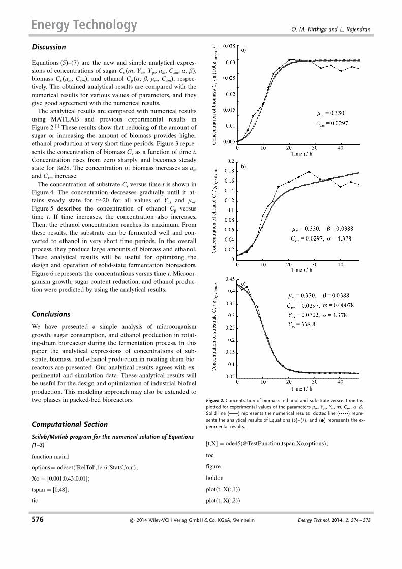
Equations (5)–(7) are the new and simple analytical expres-sions of concentrations of sugar Cs (m, Yxs, Yps, mm, Cxm, a, b),biomass Cx (mm, Cxm), and ethanol Cp (a, b, mm, Cxm), respec-tively. The obtained analytical results are compared with thenumerical results for various values of parameters, and theygive good agreement with the numerical results.

The analytical results are compared with numerical resultsusing MATLAB and previous experimental results inFigure 2.[1] These results show that reducing of the amount ofsugar or increasing the amount of biomass provides higherethanol production at very short time periods. Figure 3 repre-sents the concentration of biomass Cx as a function of time t.Concentration rises from zero sharply and becomes steadystate for tffi28. The concentration of biomass increases as mm

and Cxm increase.The concentration of substrate Cs versus time t is shown in

Figure 4. The concentration decreases gradually until it at-tains steady state for tffi20 for all values of Yxs and mm.Figure 5 describes the concentration of ethanol Cp versustime t. If time increases, the concentration also increases.Then, the ethanol concentration reaches its maximum. Fromthese results, the substrate can be fermented well and con-verted to ethanol in very short time periods. In the overallprocess, they produce large amounts of biomass and ethanol.These analytical results will be useful for optimizing thedesign and operation of solid-state fermentation bioreactors.Figure 6 represents the concentrations versus time t. Microor-ganism growth, sugar content reduction, and ethanol produc-tion were predicted by using the analytical results.

Conclusions

We have presented a simple analysis of microorganismgrowth, sugar consumption, and ethanol production in rotat-ing-drum bioreactor during the fermentation process. In thispaper the analytical expressions of concentrations of sub-strate, biomass, and ethanol production in rotating-drum bio-reactors are presented. Our analytical results agrees with ex-perimental and simulation data. These analytical results willbe useful for the design and optimization of industrial biofuelproduction. This modeling approach may also be extended totwo phases in packed-bed bioreactors.

Computational Section

Scilab/Matlab program for the numerical solution of Equations(1–3)

function main1

options= odeset(’RelTol’,1e-6,’Stats’,’on’);

Xo = [0.001;0.43;0.01];

tspan = [0,48];

tic

[t,X] = ode45(@TestFunction,tspan,Xo,options);

toc

figure

holdon

plot(t, X(:,1))

plot(t, X(:,2))

Figure 2. Concentration of biomass, ethanol and substrate versus time t isplotted for experimental values of the parameters mm, Yps, Yxs, m, Cxm, a, b.Solid line (c) represents the numerical results; dotted line (g) repre-sents the analytical results of Equations (5)–(7), and (*) represents the ex-perimental results.

576 � 2014 Wiley-VCH Verlag GmbH & Co. KGaA, Weinheim Energy Technol. 2014, 2, 574 – 578

O. M. Kirthiga and L. Rajendran

plot(t, X(:,3))

return

function [dx dt]= TestFunction(t,x)

um=0.630;cxm=0.0297;yxs=0.0702;m=0.00078;alpha=4.378;beta=0.0388;yps=338.4;

dx dt(1)=x(1)*um*(1-x(1)/cxm);

dx dt(2)= ((-1/yxs)*(x(1)*um*(1-(x(1)/cxm))))-(m*x(1))-((1/yps)*(alpha*(x(1)*um*(1-(x(1)/cxm)))+beta*x(1)));

dx dt(3)=alpha*(x(1)*um*(1-(x(1)/cxm)))+beta*x(1);

dx dt = dx dt’;

Nomenclature

Symbols

Cp [gethanol g�1dry substrate] product (ethanol) concentration

Cs [gg�1dry substrate] substrate concentration

Cx [gbiomass (100 gsubstrate)�1] biomass concentration

Cxm

[gbiomass (100 gsubstrate)�1]

maximum possible biomass con-centration

m cell maintenance constantt [h] timeYps [gethanol g

�1substrate] yield coefficient for ethanol on

the substrateYxs [gbiomass g�1

substrate] yield coefficient for cell

Greek symbols

a empirical coefficients in the ethanol productionb empirical coefficients in the ethanol productionm [h�1] specific growth ratemmax [h�1] maximum specific growth rate

Constant parameters

A0 = Cptmm � Cxmb ln Cxmð Þ � ammCxt

Figure 3. Concentration of biomass Cx versus time t is plotted using Equa-tion (5). (a) For various values of Cxm and some fixed values of mm =0.330,m=0.00078, a =4.378, b =0.0388, Yxs =0.0702, Yps =338.4. (b) For variousvalues of mm and some fixed values of Cxm =0.0297, m= 0.00078, a=4.378,b=0.0388, Yxs =0.0702, Yps =338.4.

Figure 4. Concentration of substrate Cs versus time t is plotted using Equa-tion (6). (a) For various values of Yxs and some fixed values of mm = 0.330,Cxm =0.0297, m=0.00078, a =4.378, b =0.0388, Yps = 338.4. (b) For variousvalues of mm and some fixed values of Cxm =0.0297, m= 0.00078, a=4.378,b=0.0388, Yxs =0.0702, Yps =338.4.

Energy Technol. 2014, 2, 574 – 578 � 2014 Wiley-VCH Verlag GmbH & Co. KGaA, Weinheim 577

Solid-State Fermentation for Biofuels

A1 =

CstCsmYxsYpsmm þ Cxm ln Cxmð ÞCsmYxsamm

þb

� �

þCxmmmYpsþaYxs

� �Cxt�

Cxm ln Cxmð Þ

� �

þCsmCxm ln Cxmð ÞYpsmmþmYxs

� �

A2 =� mm

Yxs�m� b

Yps� amm

Yps

A3 =mm

YxsCsmþ amm

YpsCsm

Acknowledgements

This work was supported by the Department of Science andTechnology (DST) (No. SB/SI/PC-50/2012), New Delhi,India. The authors are thankful to The Principal of TheMadura College, Madurai and The Secretary of Madura Col-lege Board, Madurai, for their encouragement.

Keywords: biofuels · bioreactors · ethanol · mathematicalmodeling · fermentation

[1] E. Q. Wang, S. Z. Li, L. Tao, X. Geng, T. C. Li, Appl. Energy 2010,87, 2839 –2845.

[2] S. R. Couto, M. A. Sanroman, J. Food Eng. 2006, 76, 291 –302.[3] A. Pandey, Biochem. Eng. J. 2003, 13, 81 –84.[4] A. Pandey, Special Section: Ferment. Sci. Technol. 1999, 77, 149 – 162.[5] A. Pandey, Process Biochem. 1991, 26, 355 – 361.[6] D. A. Mitchell, O. F. von Meien, N. Krieger, F. D. H. Dalsenter, Bio-

chem. Eng. J. 2004, 17, 15– 26.[7] R. R. Singhania, A. K. Patel, C. R.

Soccol, A. Pandey, Biochem. Eng. J.2009, 44, 13 –18.

[8] H. Chen, Modern Solid State Ferment.Theory Pract. 2013, 199 –242.

[9] C. Krishna, Critical Rev. Biotechnol.2005, 25, 1 –30.

[10] J. Sargantanis, M. N. Karim, V. G.Murphy, D. Ryoo, R. P. Tengerdy, Bio-technol. Bioeng. 1993, 42, 149 – 158.

[11] M. R. Kosseva, Food Industry Wastes2013, 77– 102.

[12] V. Bellon-Maurel, O. Orliac, P. Chris-ten, Process Biochem. 2003, 38, 881 –896.

Received: January 28, 2014Revised: February 24, 2014Published online on May 2, 2014

Figure 6. Concentration vs. time (t) is plotted using the Equations (5)–(7) forthe experimental values.[1]

Figure 5. Concentration of ethanol Cp versus time t is plotted using Equation (7). (a) For various values of a,(b) For various values of b, (c) For various values of Cxm. (d) For various values of mm and some fixed valuesof Cxm =0.0297, m=0.00078, a =4.378, b= 0.0388, Yxs =0.0702, Yps = 338.4.

578 � 2014 Wiley-VCH Verlag GmbH & Co. KGaA, Weinheim Energy Technol. 2014, 2, 574 – 578

O. M. Kirthiga and L. Rajendran