Analytical FFR

0090-6778 (c) 2013 IEEE. Personal use is permitted, but republication/redistribution requires IEEE permission. Seehttp://www.ieee.org/publications_standards/publications/rights/index.html for more information.

This article has been accepted for publication in a future issue of this journal, but has not been fully edited. Content may change prior to final publication. Citation information: DOI10.1109/TCOMM.2014.2358211, IEEE Transactions on Communications

1

A Unified Framework for the Analysis of FractionalFrequency Reuse Techniques

Azwan Mahmud and Khairi Ashour HamdiSchool of Electrical and Electronic Engineering, University of Manchester, United Kingdom

Abstract—Fractional frequency reuse (FFR) and soft frequencyreuse (SFR) systems are an efficient cellular interference man-agement technique to reduce inter-cell interference in multi-cellOFDMA networks. In this paper, a new and unified analyticalframework for performance evaluation for both systems over acomposite fading environment is presented. Explicit expressionsare obtained for the area spectral efficiency (ASE) with bothFFR and SFR; under fully-loaded and partially-loaded systems fordownlink and uplink, and in generalized frequency reuse factor.The presented numerical result provides useful system designguidelines between the two systems. It is demonstrated that SFRoutperforms FFR in a partially-loaded scenario while the oppositeis true for fully-loaded system. The mathematical model is thenextended to include the analysis of elastic data traffic in FFRsystem.

Index Terms—Area spectral efficiency, co-channel interference,fractional frequency reuse, log-normal shadowing, Nakagami fad-ing, OFDMA.

I. INTRODUCTION

The rapid growth of internet-connected mobile devices hasdriven tremendous growth in the volume of data traffic, leadingnetwork operators in search for ways to further increase therate in cellular systems. Orthogonal frequency division multipleaccess (OFDMA) has been chosen for next generation cellularsystems such as Long Term Evolution-Advance (LTE-A) as wellas next generation wireless local area networks (WLANs) todeliver high level of spectral efficiency over wideband channels[1]. In order to meet the high demand for data-rates beyondthose of 3G cellular systems, dense reuse of frequencies arerequired. In multi-cell OFDMA, the users are assigned withfrequencies which are orthogonal to each other in a referencecell, with the primary source of interferences are inter-cellinterference (ICI) from neighbouring cells. However, ICI limitsthe performance of the overall spectral efficiency of the network,especially for users near the boundary of the cells. Therefore, inorder to realize the full potential of OFDMA in a dense reusesystem, appropriate interference management techniques areessential. Traditionally, the management of ICI is handled byclassical clustering technique, e.g., frequency reuse (FR) of 3 or7 [2], [3]. Although the current cellular interference managementtechnique mitigates ICI, it limits the system throughput due tothe limited frequency resource in one cell; such technique is notgood enough for existing and future high data rate applications.

The fractional frequency reuse (FFR) system (or scheme) hasrecently been proposed as an inter-cell interference coordination

The authors are with the School of Electrical & Electronic Engineering,The University of Manchester. Sackville street, Manchester M13 9PL, UnitedKingdom. (e-mail: [email protected],[email protected])

(ICIC) technique in OFDM-based fourth generation (4G) wire-less standards such as IEEE 802.16m [4] and 3GPP-LTE Release8 and above [5], with the aim to improve the performance ofthe cellular network by having each cell allocate its resources(e.g., time, frequency, and power) in a way in which ICI inthe network is minimized [6]. The basis of the FFR schemeis to partition a cell into two or more regions: a cell-centreregion (CCR) with lower ICI due to large separation distancebetween the user and interfering base station and a cell-edgeregion (CER), experiencing a higher ICI. Therefore, the CCR isable to have a lower frequency reuse factor (FRF) or even unityfrequency reuse (UFR) while higher FRF for CER sub-bandallocation is pre-planned to not interfere with its neighbourcell-edge frequency, whilst at the same time providing goodinterference avoidance to the CCR [7].

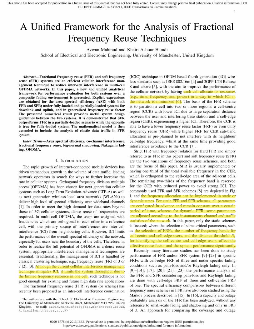
Strict FFR with frequency isolation (or Hard FFR and simplyreferred to as FFR in this paper) and soft frequency reuse (SFR)are the two variations of frequency reuse schemes, and bothare the focus of this paper. SFR is usually implemented byhaving one third of the total available frequency in the CER,which is orthogonal to the cell-edge area of the adjacent cells.The remaining two-thirds of the frequency band is reservedfor the CCR with reduced power to avoid strong ICI. Thecommonly used FFR and SFR schemes [8] are depicted in Fig.1, and the frequency allocation can be implemented in static ordynamic states. For static FFR and SFR schemes, all parametersare configured in advance and remain constant over a certainperiod of time, whereas for dynamic FFR, some parametersare adjusted according to the instantaneous channel and trafficstatistics of the network. In this paper, only the static schemesis focused; where the selection of some critical parameters, suchas the selection of FRFs, the number of frequency bands forcell-centre and cell-edge users, and the distance threshold Rtfor identifying the cell-centre and cell-edge users, affect theeffective reuse factor and the system performance significantly.

Recently, many literature studies has been done to studyperformance of FFR and/or SFR system [9]–[23] in specificFRFs with cell-edge FRF of three and under specific fadingconditions such as path-loss and/or Rayleigh fading only. In[9]–[14], [17], [20], [21], [23], the performance analysis ofthe FFR and SFR considering path-loss and Rayleigh fadingare done with cell-edge FRF of three and cell-centre FRFof one. The spectral efficiency comparisons between differentfrequency reuse schemes in FFR have also been studied using theMarkov process described in [15]. In [16], a capacity and outageprobability analysis of the FFR has been analyzed, without anyreference to small-scale fading and shadowing and only in FRFof 3. An approach for comparing the coverage and outage

Sakir

Highlight

Sakir

Highlight

Sakir

Highlight

Sakir

Highlight

Sakir

Highlight

Sakir

Highlight



2

probabilities between FFR and SFR analytically using a spatialPoisson point process (PPP) with Rayleigh fading is done [17],[18], [22]. Compared to [17], [18], [22], proposed approachis more specific since it considers a fixed cell size and not avoronoi tessellation; where performance for a typical cell ofinterest is investigated. In [21], [24] an uplink model is presentedin FFR to perform analysis of coverage, outage probabilities andcapacity, however, no generalization of the FRF is compared andin Rayleigh fading only. A comprehensive survey in inter-cellinterference coordination (ICIC) techniques has been done fordownlink in [8] and in uplink in [14], but the comparison areonly based on simulations.

The main contributions of this paper can be summarizedas follows. A new and unified mathematical framework ispresented for accurate performance evaluation of FFR and SFRin downlink and uplink scenarios. This leads to new explicitexpressions for the area spectral efficiency (ASE) in FFR andSFR systems over a composite fading environment and arbitraryFRF. The expression takes account of bandwidth proportionalitythat guarantee the number of users is proportional to the totalsystem bandwidth for the cell-centre and the cell-edge, theeffect of the power level, α, to the system performances andthe effect of the partial loading or traffic activity of the systems,as cellular system channels are not always active at all time.Furthermore, the framework for the static channel model is thenextended to study the effect of elastic data traffic (i.e., ftp traffic)in FFR system, where the users arrive at random time instantsand locations, downloading a file and leaving the system.

The remainder of this paper is organized as follows: In SectionII the general network and channel model is presented. InSection III, the downlink FFR channel model and the Signal-to-Interference-plus-Noise-ratio (SINR) is presented, followedby the new and unified expression for the FFR area spectralefficiency. The capacity for cell-centre and cell-edge in fullyloaded system is derived, and the analysis is extended to partiallyloaded systems in Section IV. Section V cover the downlinkSFR channel model, the SINR and new analysis for the SFRarea spectral efficiency. In Section VI, the FFR and SFR uplinkchannel model and capacity is derived. Section VII captured theanalysis of elastic traffic in FFR. Design issues and performancecomparisons between FFR and SFR are given in Section VIIItogether with performance of elastic traffic, and Section IXconcludes the paper.

II. SYSTEM MODEL

In this section, the general downlink network model and thebasic details of the FFR and SFR techniques is presented. Theuplink model and analysis are presented in Section VI.

A. Channel Model

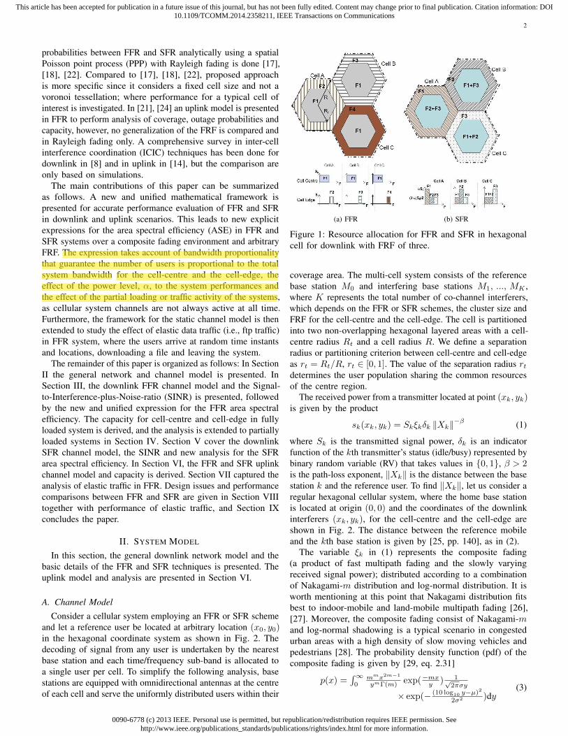
Consider a cellular system employing an FFR or SFR schemeand let a reference user be located at arbitrary location (x0, y0)in the hexagonal coordinate system as shown in Fig. 2. Thedecoding of signal from any user is undertaken by the nearestbase station and each time/frequency sub-band is allocated toa single user per cell. To simplify the following analysis, basestations are equipped with omnidirectional antennas at the centreof each cell and serve the uniformly distributed users within their

(a) FFR (b) SFR

Figure 1: Resource allocation for FFR and SFR in hexagonalcell for downlink with FRF of three.

coverage area. The multi-cell system consists of the referencebase station M0 and interfering base stations M1, ..., MK ,where K represents the total number of co-channel interferers,which depends on the FFR or SFR schemes, the cluster size andFRF for the cell-centre and the cell-edge. The cell is partitionedinto two non-overlapping hexagonal layered areas with a cell-centre radius Rt and a cell radius R. We define a separationradius or partitioning criterion between cell-centre and cell-edgeas rt = Rt/R, rt ∈ [0, 1]. The value of the separation radius rtdetermines the user population sharing the common resourcesof the centre region.

The received power from a transmitter located at point (xk, yk)is given by the product

sk(xk, yk) = Skξkδk ‖Xk‖−β (1)

where Sk is the transmitted signal power, δk is an indicatorfunction of the kth transmitter’s status (idle/busy) represented bybinary random variable (RV) that takes values in {0, 1}, β > 2is the path-loss exponent, ‖Xk‖ is the distance between the basestation k and the reference user. To find ‖Xk‖, let us consider aregular hexagonal cellular system, where the home base stationis located at origin (0, 0) and the coordinates of the downlinkinterferers (xk, yk), for the cell-centre and the cell-edge areshown in Fig. 2. The distance between the reference mobileand the kth base station is given by [25, pp. 140], as in (2).

The variable ξk in (1) represents the composite fading(a product of fast multipath fading and the slowly varyingreceived signal power); distributed according to a combinationof Nakagami-m distribution and log-normal distribution. It isworth mentioning at this point that Nakagami distribution fitsbest to indoor-mobile and land-mobile multipath fading [26],[27]. Moreover, the composite fading consist of Nakagami-mand log-normal shadowing is a typical scenario in congestedurban areas with a high density of slow moving vehicles andpedestrians [28]. The probability density function (pdf) of thecomposite fading is given by [29, eq. 2.31]

p(x) =´∞

0mmx2m−1

ymΓ(m) exp(−mxy ) 1√2πσy

× exp(− (10 log10 y−µ)2

2σ2 )dy(3)

Sakir

Highlight

Sakir

Highlight



3

‖ Xk ‖= R√

3√

(xk − rtx0)2 + (yk − rty0)2 + (yk − rty0)(xk − rtx0). (2)

where µ is the mean power in dB, σ (dB) is the shadowingstandard deviation of x, m is the Nakagami fading parameter( 1

2 ≤ m ≤ ∞) and Γ(.) is the gamma function definedby Γ(z) =

´∞0tz−1e−tdt, z ≥0. The Nakagami-m statistical

model can be used to represent many fading conditions, such asthe one-sided Gaussian distribution (m = 1/2), and Rayleighdistribution when m = 1 as a special case. Rician distributioncan also be closely approximated using the Nakagami-m whenm > 1. As m→∞, the Nakagami fading channels convergeto an additive white Gaussian noise (AWGN) channel.

B. Fractional Frequency Reuse

In FFR, the total available resources is divided between thecell-centre and the cell-edge users. Let the total number ofchannels, denoted by N , is partitioned into two orthogonal setsNI and NO which are allocated to the inner and outer users,respectively, where NI +NO = N . In addition, the cell-centreusers are assigned a FRF of ∆I whereas the cell-edge users areassigned a different FRF, ∆O, where ∆I < ∆O. It is importantto emphasize at this point that in FFR, inner and outer usersare assigned completely different set of frequencies. A commonassignment strategy in the literature of FFR is ∆I = 1 and∆O = 3, as in Fig. 1. As far as the transmit power is concerned,same transmit power is used for both inner and outer userssubbands.

C. Soft Frequency Reuse

The SFR technique is a variation of FFR scheme as illustratedin Fig. 1, employing the same dual-ring frequency strategy. InSFR, a full frequency band is reused in each cell, however,a power control is required for its operation [30]. In order toachieve this, transmission to inner and outer users have twodifferent transmit power with the cell-edge users sub-bands areallocated with a higher power amplification factor α, whereα > 1, compared to the cell-centre users.

The same frequency can be reused for either inner or outerusers, however the same frequency cannot be used for innerand outer users of the same cell. Let ∆

(SFR)O be the FRF for

the outer users. For inner users ∆(SFR)I =

∆(SFR)O

` where ` ∈{1, 2, . . .∆

(SFR)O − 1

}is a design parameter. Most common

SFR scheme assumes that ∆(SFR)O = 3 and ∆

(SFR)I = 3/2, as

shown in Fig. 1. Therefore, in SFR the inner can be assigneda non-integer FRF, depending on the design parameter `. TheSFR strategy is more bandwidth-efficient than FFR, as it reusesall available bandwidth, but it has the disadvantage of havingmore ICI interference for both the cell-edge and the cell-centreusers [31].

The next section presents an analysis of the FFR scheme,while the analysis of the SFR scheme is presented in SectionV.

Figure 2: Coordinates of interfering base stations (xk, yk) fora reference user in the cell-centre region (CCR) and in thecell-edge region (CER) in downlink with FRF=3.

III. ANALYSIS OF FRACTIONAL FREQUENCY REUSE

The instantaneous SINR for the FFR scheme is given by

SINRFFR =S0ξ0 ‖X0‖−β∑

kεK Skξkδk ‖Xk‖−β + σ2N

(4)

where ξk (k = 0, 1, ...,K) is the composite fading for the signalfrom the kth base station, σ2

N is the AWGN power and Sk isthe transmit power. In FFR schemes, S0 = S1 = ... = SK .

In (4), K represents the total number of co-channel interfererswhich depends on the cluster size and frequency reuse. It isevident from Fig. 2 that for FFR scheme, the set of interferingbase stations are K = {1, 2, ..., 18} for the cell-centre andK = {8, 10, 12, 14, 16, 18} for the cell-edge, whilst we neglectthe co-channel interferers outside of the 18 cells.

The variables δk in (4) are binary random variables thatrepresent the status of each channel

δk =

{1 if channel k is active0 otherwise.

, (5)

and we model δk by independent Bernoulli RV where theprobability, Pr (δk = 1) = q and Pr (δk = 0) = 1− q.

A. FFR Area Spectral Efficiency

The area spectral efficiency can be defined as the data ratesupported per cell [32]. We first consider evaluation of a fully-loaded cellular systems whereby all available channels are active.We then extended our analysis to partially-loaded systems wherewe determine the effect of traffic loading on the systems areaspectral efficiency.

Let CI and CO be the capacity per unit frequency inbits/sec/Hz for an arbitrary channel over the inner and outer

Sakir

Highlight

Sakir

Highlight

Sakir

Highlight

Sakir

Highlight

Sakir

Highlight

Sakir

Highlight

Sakir

Highlight



4

regions, respectively. Then the area spectral efficiency of anarbitrary channel is

η =

{CI∆I, for an inner channel

CO∆O

, for an outer channel(6)

where ∆I and ∆O are the FRFs for the inner and outer regions,respectively.

Therefore, if NO and NI are the number of channels allocatedto the inner and outer regions, then the net area spectralefficiency (ASE) in [bits/sec/Hz/cell] is

ASE =NI

NI +NO

CI∆I

+NO

NI +NO

CO∆O

. (7)

Note that if the area is normalized such that the cell area isunity then (7) is in fact the ASE in [bits/sec/Hz/m2].

In order to ensure fair allocation of channels among users inthe CCR and CER, we further assume that the number of theinner and outer channels NI and NO are allocated accordingto the average number of users in each region. Assuming that amobile can equally likely to be anywhere within a cell (assumeto be circular for ease of derivation), we have NI

∆I: NO∆O

= πR2t :

π(R2 −R2t ) or

NINO

=∆I

∆O

r2t

1− r2t

(8)

where rt = Rt/R is the normalized threshold.Combining (7) with (8) we obtain the following expression

for the area spectral efficiency of the FFR scheme

ASE =r2t

∆Ir2t + ∆O (1− r2

t )CI

+1− r2

t

∆Ir2t + ∆O (1− r2

t )CO [bits/sec/Hz/m

2].

(9)

Equation (9) is a unified expression which can be used tomeasure the effects of different FRFs and threshold distanceson the overall performance of a cellular system with fractionalfrequency reuse. The area spectral efficiency also quantifies thetrade-off between the increase in spectral efficiency by makingthe first part of (9) as large as possible, and the decrease in ca-pacity of each user resulting from the increase in ICI. Thereforethere should be an optimal value of rt which maximizes theASE in (9), where r∗t = arg maxrt ASE (rt) . The ASE in (9)is a trade-off between frequency reuse factor ∆I when rt = 1and frequency reuse factor ∆O when rt = 0. The optimum rtcan be determined using numerical methods [33], [34].

It remains to evaluate CO and CI . In Section IV a unifiedmethod for analytical evaluation of these quantities is presented.

IV. ACHIEVABLE DATA RATE

The achievable data rate for downlink FFR over compositeNakagami fading and log-normal shadowing can be generallyrepresented as [35], [36]

C = E[log2(1 +

1

ΓSINR)

](10)

where SINR is given in (4) for FFR scheme and E[.] is thestatistical expectation operation. Γ is the SINR gap to thecapacity, which denotes the amount of extra coding gain needed

to achieve Shannon capacity [37]. For the sake of simplicitythe SINR gap is assumed to be 0dB. It is important to note thatthe SINR in (10) is a ratio of a mixture of a large number ofRVs, for which a closed form of its pdf is generally difficult toobtain (if not impossible).

In the remaining of this section, a non-direct analytical methodfor efficient evaluation of CI and CO is presented.

A. Calculation of CI and COThe achievable rate of an arbitrary user can be evaluated by

computing the average in

C = E

[log2

(1 +

ξ0 ‖X0‖−β∑kεK ξkδk ‖Xk‖−β + b

)](11)

where for CO K ∈ {1, 2, ..., 18} and K ∈{8, 10, 12, 14, 16, 18} for CI . In (11), b = σ2

N/S0 is thereciprocal of the average signal to noise ratio.

The evaluation of (11) requires to calculate the averages withrespect to 3K+2 RVs, {‖X0‖ , .., ‖XK‖}, {ξ0, ξ1, ..., ξK} and{δ1, δ2, ..., δK}. In this section, we present a unified method forthe efficient computation for the averages in (10) which reducescomputational complexity. This transformation is described in[38] for Nakagami-m fading only, and this paper extended thetransformation that allows an explicit expression to be obtainedfor the capacity under composite fading and be used for FFRand SFR system evaluation, where

Lemma 1. [Hamdi [38]]For any u, v > 0

ln(

1 +u

v

)=

ˆ ∞0

1

z

(1− e−zu

)e−zvd z. (12)

Using (12), the capacity for FFR in (11) can be representedsimply as

C = log2 e

ˆ ∞0

1

z(1−M(z))MI(z)e

−bzdz (13)

where M(z) and MI(z) are the MGF of the useful andinterfering signals respectively, given by

M(z) = E[e−zξ0‖X0‖−β

](14)

andMI(z) = E

[e−z

∑Kk=1 δkξk‖Xk‖

−β]. (15)

When the coordinates of the reference user, (x0, y0), isgiven then the quantities {‖X0‖ , ‖X1‖ , ..., ‖XK‖} in down-link transmissions become non-random quantities. We obtainwhen we condition on (x0, y0) for a fully loaded cell (whereδk = 1 ∀k)

MI (z|x0, y0) = E[e−z

∑Kk=1 ξk‖Xk‖

−β |x0, y0

]=∏Kk=1 E

[e−zξk‖Xk‖

−β |x0, y0

].

(16)

As far as the calculation of the average in (14) and (16) withrespect to the composite Nakagami-m fading and log-normalshadowing is concerned, it can be shown that (see Appendix A)

M(z) ' 1√π

Ng∑n=1

Hxn

(1 + e(

√2σxn+µ) ‖X0‖−β z

m

)−m(17)



5

and

MI (z|x0, y0) '∏Kk=1

1√π

∑Ngn=1Hxn

×(

1 + e(√

2σxn+µ) zmI‖Xk‖−β

)−mI (18)

where xn and Hxn are the abscissas and weight factors of theNgth order Hermite Polynomial, respectively, and are tabulatedin Table 25.10 in [39] and mI is the interferers Nakagami fadingindex.

Finally, MI(z) can be obtained by averaging out (x0, y0) in(18).

B. Partially Loaded Cell

In the previous sections, the normalized area spectral ef-ficiency per cell is calculated based on fully-loaded cellularsystems, in which all channels in the serving base station andin all interfering base stations are assumed to be active, and thenumber of interferers therefore is constant. In this section, theeffect of partially loaded traffic conditions in the reference celland interfering cells is analyze. We obtain instead of (13)

C = log2 e´∞

01z (1−M(z))

×∏Kk=1 (1− q + q.MI(z)) e

−bzdz(19)

whereM(z) andMI(z) are given in (14) and (18), respectively,and q = Pr (δk = 1) . δk is a binary random variable that takesvalues in {0, 1} which models the kth transmitter’s (interferingbase stations) status (idle/busy). In absence of any interference,q = 0, therefore the maximum active channels is achieved whenq = 1.

In partially loaded systems the number of active users ina reference cell and the number of co-channel interferers arerandom variables, hence the area spectral efficiency in (9) forpartial load (ASE) is a function of the number of active channelsin a cell, q, now becomes

ASE = q.

[r2t

∆Ir2t + ∆O (1− r2

t ).CI

+1− r2

t

∆Ir2t + ∆O (1− r2

t ).CO

][bits/sec/Hz/m2].

(20)

V. ANALYSIS OF SOFT FREQUENCY REUSE

A. SINR

In the case of SFR, let ∆(SFR)O be the FRF of the cell-edge

users, and the total transmit power is assume to be constant. InFig. 1, the ∆

(SFR)O = 3; however, the value of ∆

(SFR)O can be

generalize to be any number bigger than the cell-centre FRF∆

(SFR)I . A transmit power control, α, is introduced to create

two different frequency bands in SFR, Sint = S0

(∆(SFR)−α

2

)and Sedge = αS0, where Sint and Sedge are the transmittedpower for the users in the cell-centre and cell-edge, respectively[10].

The interfering base stations are also separated into twoclasses: all interfering base stations transmitting to the cell-centre users on the same sub-band as the reference user (atpower Sint), and all interfering base stations transmitting to the

cell-edge users on the same sub-band as the reference user (atpower Sedge). The ratio of powers between the cell-centre tocell-edge becomes

(3−α2α

)in case of ∆

(SFR)O = 3 as in Fig.

1; therefore, adjusting the power ratio from 0 to 1 effectivelymoves the reuse factor from 3 to 1 [10].

For the case where SFR ∆(SFR)O = 3, the

SINR for SFR cell-centre reference user is givenby (21), where α is the power amplification factor,K

(1)SFR = {2, 4, 6, 7, 8, 10, 11, 12, 14, 15, 16, 18} and

K(2)SFR = {1, 3, 5, 9, 13, 17}.For the cell-edge reference user, the SINR is given by

(22), where K(3)SFR = {8, 10, 12, 14, 16, 18} and K

(4)SFR =

{1, 2, 3, 4, 5, 6, 7, 9, 11, 13, 15, 17}.

B. SFR Area Spectral Efficiency

In the case of SFR, a sub-carrier can be used for both innerand outer regions of different cells. Then in any ∆

(SFR)O cells,

each sub-carrier is reused in only one outer region, but can beused in any inner region of the remaining ∆

(SFR)O − 1 cells.

Therefore

ASESFR =`C

(SFR)I + C

(SFR)O

∆(SFR)O

(23)

where ` ∈{

1, 2, . . .∆(SFR)O − 1

}is a design parameter. Note

that in most common SFR arrangements (e.g. SFR with threecell clusters as illustrated in Fig. 1) ∆

(SFR)O = 3 and ` = 2

[30].In order to ensure fairness among users within a cell, we can

set` = min

(⌈r2t

1−r2t

⌉,∆

(SFR)O − 1

). (24)

Substituting (24) in (23) present us with a unified expressionfor SFR which can be used to study the effects of differentFRFs and threshold distances on the overall performance of acellular system.

C. Calculation of C(SFR)I and C(SFR)

O and Partial Loading

Using (13) and SINR in (21) and similar derivation for partialloading in FFR, we can show that

C(SFR)I = log2e

ˆ ∞0

1

z(1−M(z))

K(1)∏k=1

(1− q + q.MC(z))

×K(2)∏k=1

(1− q + q.ME(z)) e−bzdz (25)

whereM(z),MC(z),ME(z) is the MGF of the useful signal,the interfering signals from the neighbouring CER channels andthe interfering signals from the neighbouring CCR channels,respectively, given by

M(z) ' 1√π

Ng∑n=1

Hxn

(1 + e(

√2σxn+µ)

(3− α

2

)‖X0‖−β z

m

)−m(26)

MC(z|x0, y0) '∏kεK(1)

1√π

∑Ngn=1Hxn

×(

1 + e(√

2σxn+µ)α zmI‖Xk‖−β

)−mI(27)

Sakir

Highlight



6

SINRCCSFR =

(3−α

2

)ξ0 ‖X0‖−β

α∑kεK

(1)SFR

ξkδk ‖Xk‖−β +(

3−α2

)∑kεK

(2)SFR

ξkδk ‖Xk‖−β + b(21)

SINRCESFR =

αξ0 ‖X0‖−β(3−α

2

)∑kεK

(3)SFR

ξkδk ‖Xk‖−β + α∑kεK

(4)SFR

ξkδk ‖Xk‖−β + b(22)

and

ME(z|x0, y0) '∏kεK(2)

1√π

∑Ngn=1Hxn

×(

1 + e(√

2σxn+µ)(

3−α2

)zmI‖Xk‖−β

)−mI.

(28)Likewise, similar expressions for C(SFR)

O can be derived.In partially loaded systems, the area spectral efficiency in (9)

for partial load (ASE) for SFR now becomes

ASE = q.

[`C

(SFR)I + C

(SFR)O

∆(SFR)O

][bits/sec/Hz/m2]. (29)

VI. UPLINK DISCUSSION

The previous results on downlink capacity of SFR and FFRcan be extended to include uplink scenarios. While interferencein downlink transmissions comes from fixed sources (basestations), interference in uplink comes from users that aredistributed randomly throughout the neighbouring cells. For thesake of uplink analysis, the cells are assume to be of circularshape.

In the case of uplink FFR, the instantaneous SINR of areference user at random distance r0 can be represented as

SINR(UL)FFR (x0, y0) =

r−β0 ξ0∑Kk=1 ξk (D

2 + r2k − 2rkD cos θk)−β/2 + b

(30)with D being the distance between two adjacent cells, (rk, θk)is the polar coordinates of the kth interferer (relative to its basestation).

The pdf of the reference user in the CCR of FFR or SFRschemes at radius r and angle θ relative to their base stations is

pr(r) = 2r/R2t (31)

andpθ(θ) = 1/2π (32)

where 0 ≤ r ≤ Rt and 0 ≤ θ ≤ 2π. Similarly, the pdf for thereference user in the CER that lies between Rt and R is givenby

pr(r) = 2r/(R2 −R2t ) (33)

andpθ(θ) = 1/2π (34)

where Rt ≤ r ≤ R and 0 ≤ θ ≤ 2π.The uplink capacity of the FFR reference user under com-

posite Nakagami-m fading and log-normal shadowing in CERcan be represented

C(UL)O = log2 e

´∞0

1z

(1−M(CE)(z)

)×M(CE)

I (z)e−zbdz(35)

where

M(CE)(z) = 1π

´ RRt

1√π

∑Ngn=1Hxn

×(

1 +zr−β0

m e(√

2σxn+µ))−m

2rR2−R2

t.dr

(36)

and

M(CE)I (z) =

[1π

´ 2π

0

´ RRt

1√π

∑Ngn=1Hxn

(1 + e(

√2σxn+µ) z

mI

×(D2 + r2

k − 2rkD cos θk)−β/2)−mI) r

R2−R2t.dr.dθ

]K(37)

with K is coming from the nearest 6 co-channel cells.The uplink capacity for FFR reference user in CCR is

C(UL)I = log2 e

´∞0

1z

(1−M(CC)(z)

)×M(CC)

I (z)e−zbdz(38)

where

M(CC)(z) = 1π

´ Rt0

1√π

∑Ngn=1Hxn

×(

1 +zr−β0

m e(√

2σxn+µ))−m

2rR2tdr

(39)

and

M(CC)I (z) =

[1π

´ 2π

0

´ Rt0

1√π

∑Ngn=1Hxn

(1 + e(

√2σxn+µ) z

mI

×(D2 + r2

k − 2rkD cos θk)−β/2)−mI) r

R2t

dr dθ]K

(40)with K is coming from 18 co-channel cells.

Similar results can be obtained in case of SFR schemes.

VII. ELASTIC TRAFFIC

The analysis of previous section were based on static trafficscenarios, where all transmissions from (busy) stations arecontinuous. In this section, the FFR framework is extendedto elastic traffic where users arrive at random time instants,downloading a file and leaving the system [40], [41]. In thiscase, the actual set of active users is dynamic and varies as arandom process where new data flows are initiated and otherscomplete. In this paper, a widely used model in the analysisof cellular data networks is adopted whereby each station isrepresented by an independent M/G/1/PS queue [40], [42], [43].

Let the number of active users at location x (in an arbitrarycell) be represented by a Poisson arrival of intensity of λ (x) dx[flow/s]. The users arriving in the cell require to transmit somevolumes of data which are independent identically distributedrandom variables of mean 1

µ [bits/flow] . The traffic demandin a given area A is the product of the flow arrival rate and themean flow volume

ρ = λ/µ [bits/s] (41)



7

where λ =´Aλ(x)A dx [flow/s] is the average flow intensity in

area A. On the other hand, the volume of data is proportionalto the average transmission time which is proportional to theaverage of the reciprocal of the transmission rate

1

µ= E

[1

BC (x)

](42)

where B is the total bandwidth allocated to area A and C (x) =E [log2 (1 + SINR) |x] is the normalized channel capacity inbits/s/Hz for users at distance x from the base station.

In addition, it is known from queuing theory thatPr (a queue is busy) = max (1, ρ) . Therefore, in orderto take into account the co-channel interference gener-ated by elastic traffic in different co-channel cells, weset Pr (base station i is transmitting at an arbitrary time) =max (ρi, 1) . Accordingly, in light of (19), the ergodic capacityof a user at (x, θ) in the presence of K co-channel interfererscan be expressed as follows

C (x, θ, ρ1, . . . , ρK) = log2 e

ˆ ∞0

1

z

(1−M(z.x−β)

)×

K∏k=1

(1−max (1, ρk)

+ max (1, ρk)MI(z, x, θ)) e−bzdz (43)

where M(z) and MI(z, x, θ) are given in (17) and (18),respectively.

In this respect, for FFR, the number of active users in the cell-centre (with subscript I) and the cell-edge (with subscript O)behave as two independent single-server queues with parametersλI , CI , BI and λO, CO, BO respectively. Furthermore, weassume that all cells experience identical loads ρI and ρO.Hence, from (41) and (42)

ρI = λI

ˆ rt

0

ˆ 2π

0

1

BICI (x, θ, ρI)

dθ

2π

2xdx

r2t

(44)

and

ρO = λO

ˆ 1

rt

ˆ 2π

0

1

BOCO (x, θ, ρO)

dθ

2π

2xdx

1− r2t

. (45)

Here, for the sake of simplicity, we have assumed circular cellsand therefore polar coordinates are used instead of hexagonalcoordinates.

According to M/G/1/PS, the base station is stable if bothρI < 1 and ρO < 1 (the distribution of number of active userstends to a finite stationary distribution). The cell capacity isdefined as the maximum traffic intensity for which the cell isnot saturated. The capacity of the inner and outer regions areobtained from (44) and (45) as follows

λI = maxρI

ρIBIr2t

(1

2π

ˆ rt

0

ˆ 2π

0

2x

CI (x, θ, ρI)dθdx

)−1

(46)and

λO = maxρO

ρOBO(1− r2

t

)( 1

2π

ˆ 1

rt

ˆ 2π

0

2x

CO (x, θ, ρO)dθdx

)−1

.

(47)Hence, the aggregate data transmission per cell is

λ = λI + λO. (48)

Let the total bandwidth in a cell be partitioned according tothe following (fair) policy

BI : BO = r2t : 1− r2

t (49)

where BI = NI∆I

and BO = NO∆O

and NI and NO are,respectively, the total bandwidth allocated to inner and outerregions in the cluster. We get from (49)

NINO

=∆I

∆O

r2t

1− r2t

(50)

which results in the following bandwidth allocations

BI =NI∆I

= Nr2t

∆Ir2t + ∆O (1− r2

t )(51)

and

BO =NO∆O

= N

(1− r2

t

)∆Ir2

t + ∆O (1− r2t )

(52)

where N = NI +NO is the total system bandwidth.Let λ̃ = λ

N be the normalized capacity in bits/s/Hz/cell (whichis equivalent to the area spectral efficiency for static traffic).Then from (51), (52), (46), (47) and (48)

λ̃ =r4t

∆Ir2t + ∆O (1− r2

t )max

0<ρI<1ρI

×(

1

2π

ˆ rt

0

ˆ 2π

0

2x

CI (x, θ, ρI)dθdx

)−1

+

(1− r2

t

)2∆Ir2

t + ∆O (1− r2t )

× max0<ρO<1

ρO

(1

2π

ˆ 1

rt

ˆ 2π

0

2x

CO (x, θ, ρO)dθdx

)−1

(53)

Equation (53) is a new unified expression for FFR spectralefficiency (as measured in terms of the capacity normalized tothe total system bandwidth) in the case of elastic traffic. Thiscan be used to obtain the optimum threshold distance rt whichmaximizes the overall spectral efficiency of the FFR system.Numerical results for FFR with elastic traffic are presented anddiscussed in Section VIII.

VIII. DESIGN ISSUES AND PERFORMANCE COMPARISON

In this chapter, analysis of the FFR and SFR schemes is donebased on analytical expressions derived in previous chaptersand then compared to a Monte Carlo simulations. The systemparameters used in the analytical and simulation are shownin Table 1. Assume that the maximum power per cell for theFFR and the SFR is constant; the FFR maximum power percell is split equally between two frequency partitions, the cellcentre and the cell-edge, while for SFR, the maximum power

Table I: System Parameters

Setup Criteria ParameterNumber of Cells 19

Cell Radius 1kmAntenna SISO

Path loss exponent 3,4Fast Fading Model Nakagami-m, m ≥ 1

2Slow Fading Model Log-normal with µ = 0 and σ = 2, 4, 8

SNR Varies between 0 to 30dBTransmit Power of BS Normalize to 1Threshold distance Rt Variable

User distribution uniform



8

0.1 0.2 0.3 0.4 0.5 0.6 0.7 0.8 0.90.3

0.35

0.4

0.45

0.5

0.55

0.6

0.65

0.7

0.75

0.8

Normalize radius (rt)

ASE

[B

its/s

/Hz/

km2 ]

FFRSimulations

∆I=1,∆

O=3

∆I=1,∆

O=4

∆I=1,∆

O=7

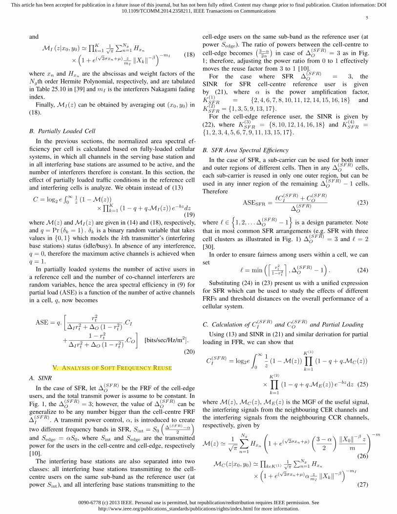
Figure 3: Area spectral efficiency for FFR against normalizeradius rt with different CCR and CER FRF (∆I and ∆O) withm = 1, σ = 2 and at SNR 2dB.

per cell is split between three frequency partitions, two partsfor cell-centre and one part for the cell-edge. In order to ensurethat we are using constant power, we normalize the SFR powerper frequency band (S0SFR) to FFR power per frequency band(S0FFR), where S0FFR = 3

2S0SFR .The Nakagami-m parameters are chosen for m ≥ 1/2; where

a special case for Rayleigh fading is when m = 1. In log-normal, the shadowing parameter is set at µ = 0 and thestandard deviation used is between 2 to 8. The signal-to-noiseratio (SNR), 1

b , is varies between 0dB and 30dB. From thegeometry of the network, Fig. 2 shows that the main downlinkinterferers originate from the first tier and the second tier basestations for the cell-centre, for both FFR and SFR. The selectionof two main ring of interfering cells is to ensure that the effectof both of the cell-centre and cell-edge interferers is considered.The reference user coordinates for the cell-edge and the cell-centre is selected for the worst location, located at the vertex ofthe hexagonal cell, at the point

√3R(

13 ,

13

)and√

3Rt(

13 ,

13

),

respectively. Without loss of generality, the total number ofsub-bands N and the cell radius R is normalized to one.

A. Downlink Discussion

In the case of FFR with 4O = 1 and 4I = 3, the interferingbase stations, K = {1, 2, ..., 18} for FFR cell-centre, and K ={8, 10, 12, 14, 16, 18} for the cell-edge. The second tier basestations will become the first tier interferers for the cell-edgeusers. The cell-edge interfering base stations will provide 33% ofdownlink interferers, while cell-centre base station will provide100% interferers, based on the same distance for both the cell-edge and cell-centre. Without loss of generality, the total numberof sub-bands N and the cell radius R is normalized to one. Thenormalized radius rt is varied between 0.1 and 0.95 correspondsto the 1% to 90% of the cell area.

For the SFR ∆(SFR)O = 3, the interfering base station for

the cell-centre users comes from the interfering base stationsthat are using the sub-bands for its inner band, K(1)

SFR = {2,

0.1 0.2 0.3 0.4 0.5 0.6 0.7 0.8 0.9

0.3

0.35

0.4

0.45

0.5

0.55

0.6

0.65

0.7

0.75

0.8


ASE

[B

its/s

/Hz/

km2 ]

AnalyticalSimulations

α=1.5,2,2.5

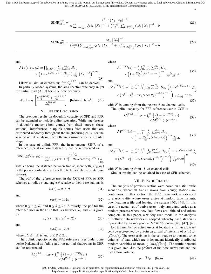
Figure 4: Area spectral efficiency for SFR against normalizeradius rt with different power amplification factor (α)with∆

(SFR)O = 3, m = 1 and σ = 2 and SNR at 2dB.

0.1 0.2 0.3 0.4 0.5 0.6 0.7 0.8 0.9

0.3

0.4

0.5

0.6

0.7

0.8

0.9

1

1.1


ASE

[B

its/s

/Hz/

km2 ]

FFRSFR (SNR 15dB)SFR(SNR 30dB)Reuse−3(SNR=15dB)Reuse−1 (SNR=15dB)

SNR=15,30dB

α=1.5

α=2.5

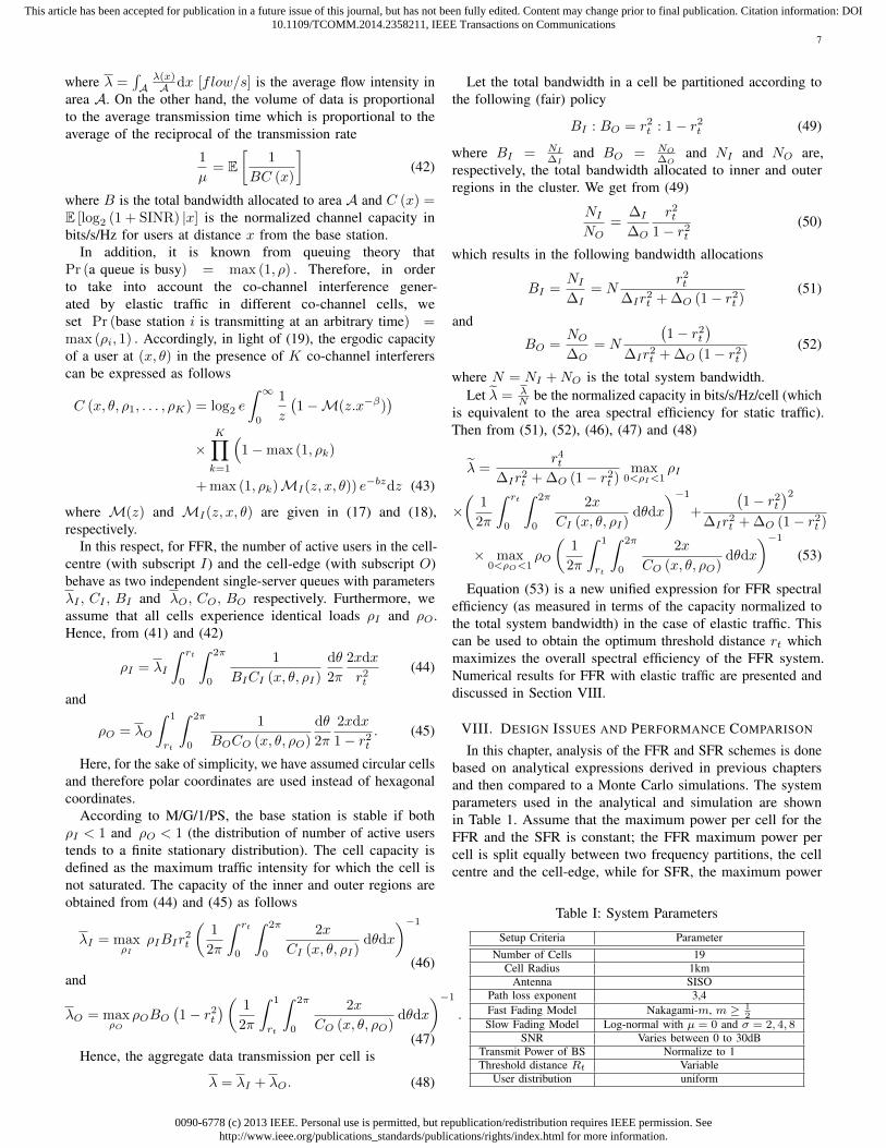
Figure 5: Area spectral efficiency for FFR, SFR, Reuse-1 andReuse-3 against normalize radius at high SNR.

4, 6, 7, 8, 10, 11, 12, 14, 15, 16, 18} and from the basestations using the sub-bands for its outer bands, K(2)

SFR ={1, 3, 5, 9, 13, 17}, with the power amplification factor of α and(

3−α2α

), respectively. The interfering base stations for the cell-

edge users will come from set of interfering base stations thatare using the inner sub-band, K(3)

SFR = {8, 10, 12, 14, 16, 18}and the base stations using the sub-bands for its outer sub-band,K

(4)SFR = {1, 2, 3, 4, 5, 6, 7, 9, 11, 13, 15, 17}, with the power

amplification factor of(

3−α2α

)and α, respectively.

Effect of different FRF in CCR and CER to the systemsperformances: In Figs. 3 and 4, the analytical and simulationresults for the normalized area spectral efficiency against rtare presented for both the FFR and SFR schemes, respectively.Using (9) and (23) simplifies greatly the evaluation of areaspectral efficiency of the FFR and SFR systems in the presenceof different types of interference. The direct analytical results are



9

−10 −5 0 5 10 15 20 25 300.2

0.3

0.4

0.5

0.6

0.7

0.8

0.9

1

1.1

1.2

SNR (dB)

ASE

[B

its/s

/Hz/

km2 ]

SFRFFR

rt=0.8,0.5,0.3

rt=0.3,0.8,0.3

Figure 6: FFR and SFR area spectral efficiency against SNRfor different rt.

compared to the simulations with 105 iterations. The accuracy ofthe mathematical model is highlighted by the closed match of thecurves with the simulation results. Denote that the computationalcomplexity of the average in (11) is greatly simplified when(13), (17) and (18) is employed, with only a single integral.Equation (11) can be solved using conventional quadrature rulemethod or the Gauss-Chebyshev Quadrature integration rule.

Fig. 3 shows different combinations of FRF 4O for theFFR schemes, with FRF 4I = 1. The ASE for the 4O = 3is the highest as compared to 4O = 4 or 4O = 7. Thesebehaviours are due to fact that the area spectral efficiency in (9),varies linearly with the allocated channels while the capacityis logarithmically proportional to the SINR. Fig. 4 shows theSFR area spectral efficiency with different power amplificationfactor α. It is observed that the overall area spectral efficiencyin a cell using (23) decreases as we increases the cell-edgepower factor, while reuse factor of 1 in the CCR increasesthe cell spectral efficiency, it also gives a higher possibility ofperformance outage. The generalized expressions in (7) and (23)can easily extended to include various frequency partitioningused for the chosen scheme. For example, FFR with three layersof sub-bands in a concentric circle, the FFR cell-centre sub-bands can be set to 4I = 1, the second sub-bands 4(1)

O = 3

and the third sub-bands (cell-edge), 4(2)O = 7. The ASE in (7)

now becomes

ASE = NINI+N

(1)O +N

(2)O

CI∆I

+

N(1)O

NI+N(1)O +N

(2)O

C(1)O

∆(1)O

+N

(2)O

NI+N(1)O +N

(2)O

C(2)O

∆(2)O

(54)

where N (1)O and N (2)

O are number of channels allocated to thesecond and third concentric circle from the reference base station.Many other possibilities for combining the frequency reuse canbe performed using (54).

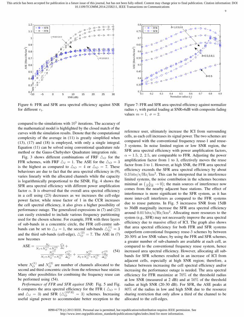
Performance of FFR and SFR against SNR: Fig. 5 and Fig.6 compares the area spectral efficiency for the FFR ( 4O = 1

and 4I = 3) and SFR (4(SFR)O = 3) schemes. Increasing

useful signal power to accommodate better reception to the

0.1 0.2 0.3 0.4 0.5 0.6 0.7 0.8 0.90.3

0.35

0.4

0.45

0.5

0.55

0.6

0.65

0.7

0.75

0.8


ASE

[B

its/s

/Hz/

km2 ]

FFRSFR

δ=0.5,0.8,1

δ=1,0.9,0.8

δ=0.5

Figure 7: FFR and SFR area spectral efficiency against normalizeradius rt with partial loading at SNR=6dB with composite fadingvalues m = 1, σ = 2.

reference user, ultimately increase the ICI from surroundingcells, as each cell increases its signal power. The two schemes arecompared with the conventional frequency reuse-1 and reuse-3 systems. In noise limited region or low SNR region, theSFR area spectral efficiency with power amplification factors,α = 1.5, 2, 2.5, are comparable to FFR. Adjusting the poweramplification factor from 1 to 3, effectively moves the reusefactor from 3 to 1. However, at high SNR, the FFR area spectralefficiency exceeds the SFR area spectral efficiency by about0.3 bits/s/Hz/km2. This can be interpreted that in interferencelimited systems, the noise contribution in the schemes becomesminimal as

(1

SNR → 0); the main sources of interference now

comes from the nearby adjacent base stations. The effect ofinterference is more significant to the SFR system, as it hasmore inter-cell interferers as compared to the FFR systemsdue to reuse patterns. In Fig. 5 increasess SNR from 15dBto 30dB marginally increase the SFR area spectral efficiencyaround 0.01 bits/s/Hz/km2. Allocating more resources to thesystem (e.g., SFR) may not necessarily improve the area spectralefficiency due to massive effect of ICI. The graph also showsthat area spectral efficiency for both FFR and SFR systemsoutperform conventional frequency reuse-3 schemes by between20-30% at low SNR values; by using the FFR and SFR schemes,a greater number of sub-channels are available at each cell, ascompared to the conventional frequency reuse system, henceincreased area spectral efficiency. However, allocating all sub-bands for SFR schemes resulted in an increase of ICI fromadjacent cells, especially at high SNR region; therefore, abalance between increasing the cell spectral efficiency and/orincreasing the performance outage is needed. The area spectralefficiency for FFR maximize at 70% of the threshold radiusat low SNR (measured at 2 dB) and at 50% of the thresholdradius at high SNR (20-30 dB). For SFR, the ASE peaks at80% of the radius in low and high SNR due to the resourcesharing restriction that only allow a third of the channel to beallocated to the cell-edges.



10

0.1 0.2 0.3 0.4 0.5 0.6 0.7 0.8 0.9

0.6

0.65

0.7

0.75

0.8

0.85

0.9

Normalize Radius (rt)

ASE

[B

it/s/

Hz/

km2 ]

FFR with m=1FFR with m=5

mI=1,2,5

mI=1,2,5

(a) FFR

0.1 0.2 0.3 0.4 0.5 0.6 0.7 0.8 0.90.3

0.35

0.4

0.45

0.5

0.55

0.6

0.65

0.7


ASE

[B

its/s

/Hz/

km2 ]

Analytical m=1Analytical m=5

mI=5,2

mI=5,2

(b) SFR

Figure 8: FFR and SFR area spectral efficiency against normalize radius rt with different Nakagami fading index m = 1, 5 andmI = 1, 2, 5.

0.1 0.2 0.3 0.4 0.5 0.6 0.7 0.8 0.90.6

0.65

0.7

0.75

0.8

Normalize Radius (rt)

ASE

[B

its/s

/Hz/

km2 ]

FFR

σ=0,2,4,8

(a) FFR

0.1 0.2 0.3 0.4 0.5 0.6 0.7 0.8 0.9

0.3

0.35

0.4

0.45

0.5

0.55

0.6

0.65

0.7

0.75

0.8


ASE

[B

its/s

/Hz/

km2 ]

SFR

σ=2,4,8

(b) SFR

Figure 9: FFR and SFR area spectral efficiency against normalize radius rt with different value of σ = 2, 4, 8.

Partial traffic loading: In partially-loaded network, thenumber of active channels in the cells depends on the trafficloading factor δk. In Fig. 7, partially-loaded systems have lowerarea spectral efficiency than fully-loaded systems, since the areaspectral efficiency increases as the active channels increases.From (20), although individual user achieved higher rates inpartially-loaded systems due to lower ICI from co-channelinterferers; this effect is offset by the fact that with feweractive channels, as only a fraction of allocated bandwidth isin used. At loading factor δk ≤ 0.8, it is observed that SFRscheme has better ASE than FFR and at δk = 0.5, significantSFR improvement to FFR ASE of 0.2 bits/s/Hz/km2 is seen;mainly due the effective number of active interfering channelsfrom all 18 neighbouring cells reduces for SFR in comparisonto only 6 for FFR.

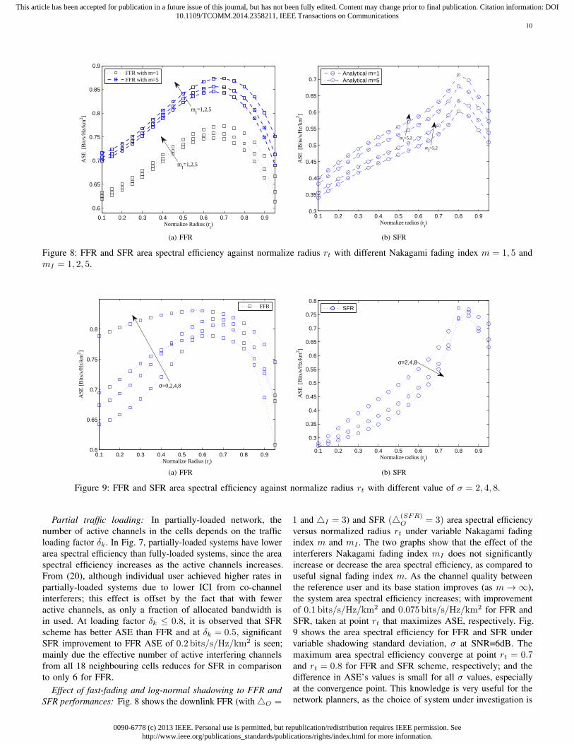
Effect of fast-fading and log-normal shadowing to FFR andSFR performances: Fig. 8 shows the downlink FFR (with4O =

1 and 4I = 3) and SFR (4(SFR)O = 3) area spectral efficiency

versus normalized radius rt under variable Nakagami fadingindex m and mI . The two graphs show that the effect of theinterferers Nakagami fading index mI does not significantlyincrease or decrease the area spectral efficiency, as compared touseful signal fading index m. As the channel quality betweenthe reference user and its base station improves (as m→∞),the system area spectral efficiency increases; with improvementof 0.1 bits/s/Hz/km2 and 0.075 bits/s/Hz/km2 for FFR andSFR, taken at point rt that maximizes ASE, respectively. Fig.9 shows the area spectral efficiency for FFR and SFR undervariable shadowing standard deviation, σ at SNR=6dB. Themaximum area spectral efficiency converge at point rt = 0.7and rt = 0.8 for FFR and SFR scheme, respectively; and thedifference in ASE’s values is small for all σ values, especiallyat the convergence point. This knowledge is very useful for thenetwork planners, as the choice of system under investigation is



11

0.1 0.2 0.3 0.4 0.5 0.6 0.7 0.8 0.9

0.8

1

1.2

1.4

1.6

1.8

2

2.2

2.4

Normalize radius rt

ASE

[B

it/s/

Hz/

km2 ]

FFRSFRSimulation

m=1,2,5

m=1,2,5

Figure 10: Uplink FFR and SFR area spectral efficiency againstrt under composite fading with Nakagami fading index m =1,2,5, σ = 2 and SNR at 2dB.

less dependent on the user fading parameter m and the interferersfading parameter mI .

B. Uplink Discussion

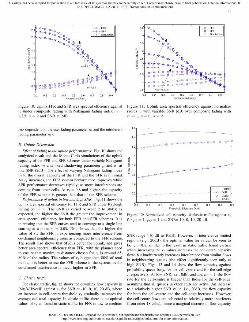
Effect of fading to the uplink performances: Fig. 10 shows theanalytical result and the Monte Carlo simulations of the uplinkcapacity of the FFR and SFR schemes under variable Nakagamifading index m and fixed shadowing parameter µ and σ, atlow SNR (2dB). The effect of varying Nakagami fading indexm to the overall capacity of the FFR and the SFR is minimal.As rt increases, the FFR system performance improves whileSFR performance decreases rapidly; as more interferences arecoming from other cells. At rt = 0.8 and higher, the capacityof the FFR scheme is greater than that of the SFR scheme.

Performance of uplink in low and high SNR: Fig. 11 shows theuplink area spectral efficiency for FFR and SFR under Rayleighfading (m = 1). The SNR is varied between 2 to 30dB; asexpected, the higher the SNR the greater the improvement inarea spectral efficiency for both FFR and SFR schemes. It isinteresting that the SFR curves tend to converge to a single linestarting at a point rt = 0.65. This shows that the higher thevalue of rt, the SFR is experiencing more interference fromco-channel neighbouring users as compared to the FFR scheme.The result also shows that SFR is better for uplink, and givesbetter area spectral efficiency than FFR, with the planner needto ensure that maximum distance chosen for rt is around 65-80% of the radius. The values of rt bigger than 80% of totalradius, it is better to use the FFR scheme in the system, as theco-channel interference is much higher in SFR.

C. Elastic traffic

For elastic traffic, fig. 12 shows the downlink flow capacity in[bits/s/Hz/cell] against rt for SNR at -10, 0, 10, 20 dB, wherean increase in cell-centre threshold rt gradually increases theaverage cell total capacity. In elastic traffic, there is no optimalvalues of rt as found in static traffic for FFR in low to medium

0.1 0.2 0.3 0.4 0.5 0.6 0.7 0.8 0.9

0.5

1

1.5

2

2.5

3

3.5

4

4.5


ASE

[B

it/s/

Hz/

km2 ]

FFRSFRSimulations

SNR=2,6,15,30

SNR=2,6,15,30

Figure 11: Uplink area spectral efficiency against normalizeradius rt with variable SNR (dB) over composite fading withm = 1, µ = 0, σ = 2.

0.1 0.2 0.3 0.4 0.5 0.6 0.7 0.8 0.90

0.2

0.4

0.6

0.8

1

1.2

1.4

1.6

Threshold Distance [Km]

Flo

w c

apac

ity

−10dB0dB10dB20dB

Figure 12: Normalized cell capacity of elastic traffic against rtfor ρI = 1, ρO = 1 and SNR=-10, 0, 10, 20 dB.

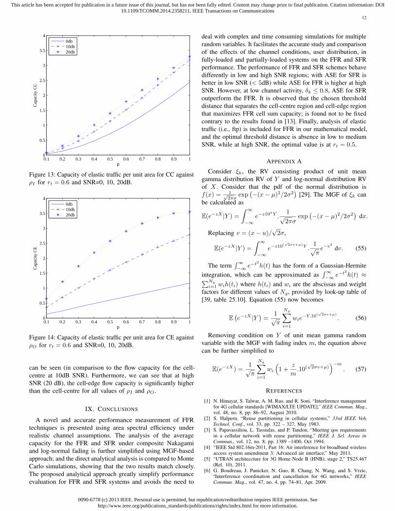
SNR range (-10 dB to 10dB). However, in interference limitedregion, (e.g., 20dB), the optimal value for rt can be seen tobe rt = 0.5, similar to the result in static traffic found earlier;where increasing the rt values increases the cell-centre capacityflows but inadvertently increases interference from similar flowsin neighbouring queues (the effect significantly seen only athigh SNR). Figs. 13 and 14 show the flow capacity againstprobability queue busy, for the cell-centre and for the cell-edge, respectively. At low SNR, i.e., 0dB, and ρO, ρI = 1, the flowrate for the cell-centre is bigger than those for the cell-edge,assuming that all queues in other cells are active. An increaseto a relatively higher SNR value, i.e., 20dB, the flow capacityfor both the cell-centre and the cell-edge increases. However,the cell-centre flows are subjected to relatively more interferers(from other 18 cells), hence a marginal increase in flow capacity



12

0.1 0.2 0.3 0.4 0.5 0.6 0.7 0.8 0.9 10

0.5

1

1.5

2

2.5

3

3.5

4

ρ

Cap

acity

CC

0db10db20db

Figure 13: Capacity of elastic traffic per unit area for CC againstρI for rt = 0.6 and SNR=0, 10, 20dB.

0.1 0.2 0.3 0.4 0.5 0.6 0.7 0.8 0.9 10

0.5

1

1.5

2

2.5

3

3.5

4

ρ

Cap

acity

CE

0db10db20db

Figure 14: Capacity of elastic traffic per unit area for CE againstρO for rt = 0.6 and SNR=0, 10, 20dB.

can be seen (in comparison to the flow capacity for the cell-centre at 10dB SNR). Furthermore, we can see that at highSNR (20 dB), the cell-edge flow capacity is significantly higherthan the cell-centre for all values of ρI and ρO.

IX. CONCLUSIONS

A novel and accurate performance measurement of FFRtechniques is presented using area spectral efficiency underrealistic channel assumptions. The analysis of the averagecapacity for the FFR and SFR under composite Nakagamiand log-normal fading is further simplified using MGF-basedapproach; and the direct analytical analysis is compared to MonteCarlo simulations, showing that the two results match closely.The proposed analytical approach greatly simplify performanceevaluation for FFR and SFR systems and avoids the need to

deal with complex and time consuming simulations for multiplerandom variables. It facilitates the accurate study and comparisonof the effects of the channel conditions, user distribution, infully-loaded and partially-loaded systems on the FFR and SFRperformance. The performance of FFR and SFR schemes behavedifferently in low and high SNR regions; with ASE for SFR isbetter in low SNR (< 5dB) while ASE for FFR is higher at highSNR. However, at low channel activity, δk ≤ 0.8, ASE for SFRoutperform the FFR. It is observed that the chosen thresholddistance that separates the cell-centre region and cell-edge regionthat maximizes FFR cell sum capacity; is found not to be fixedcontrary to the results found in [13]. Finally, analysis of elastictraffic (i.e., ftp) is included for FFR in our mathematical model,and the optimal threshold distance is absence in low to mediumSNR, while at high SNR, the optimal value is at rt = 0.5.

APPENDIX A

Consider ξk, the RV consisting product of unit meangamma distribution RV of Y and log-normal distribution RVof X . Consider that the pdf of the normal distribution isf(x) = 1√

2πσexp

(−(x− µ)2/2σ2

)[29]. The MGF of ξk can

be calculated as

E(e−zX |Y ) =

ˆ ∞−∞

e−z10xY .1√2πσ

exp(−(x− µ)2/2σ2

)dx.

Replacing v = (x− u)/√

2σ,

E(e−zX |Y ) =

ˆ ∞−∞

e−z10(√

2σv+µ)Y .1√πe−v

2

dv. (55)

The term´∞−∞ e−t

2

h(t) has the form of a Gaussian-Hermiteintegration, which can be approximated as

´∞−∞ e−t

2

h(t) ≈∑Ngi=1 wih(ti) where h(ti) and wi are the abscissas and weight

factors for different values of Ng , provided by look-up table of[39, table 25.10]. Equation (55) now becomes

E(e−zX |Y

)=

1√π

Ng∑i=1

wie−Y.10(

√2σv+µ)

. (56)

Removing condition on Y of unit mean gamma randomvariable with the MGF with fading index m, the equation abovecan be further simplified to

E(e−zX) =1√π

Ng∑i=1

wi

(1 +

z

m.10(√

2σv+µ))−m

. (57)

REFERENCES

[1] N. Himayat, S. Talwar, A. M. Rao, and R. Soni, “Interference managementfor 4G cellular standards [WIMAX/LTE UPDATE],” IEEE Commun. Mag.,vol. 48, no. 8, pp. 86–92, August 2010.

[2] S. Halpern, “Reuse partitioning in cellular systems,” 33rd IEEE Veh.Technol. Conf., vol. 33, pp. 322 – 327, May 1983.

[3] S. Papavassiliou, L. Tassiulas, and P. Tandon, “Meeting qos requirementsin a cellular network with reuse partitioning,” IEEE J. Sel. Areas inCommun,, vol. 12, no. 8, pp. 1389 –1400, Oct 1994.

[4] “IEEE Std 802.16m-2011, Part 16: Air interference for broadband wirelessaccess system amendment 3: Advanced air interface,” May 2011.

[5] “UTRAN architeccture for 3G Home Node B (HNB); stage 2,” TS25.467(Rel. 10), 2011.

[6] G. Boudreau, J. Panicker, N. Guo, R. Chang, N. Wang, and S. Vrzic,“Interference coordination and cancellation for 4G networks,” IEEECommun. Mag., vol. 47, no. 4, pp. 74–81, Apr. 2009.



13

[7] R. Giuliano, C. Monti, and P. Loreti, “WiMAX fractional frequency reusefor rural environments,” IEEE Trans. Wireless Commun., vol. 15, no. 3,pp. 60 –65, Jun. 2008.

[8] A. Hamza, S. Khalifa, H. Hamza, and K. Elsayed, “A survey on inter-cellinterference coordination techniques in OFDMA-based cellular networks,”IEEE Commun. Surveys Tuts., vol. 15, no. 4, pp. 1642–1670, Apr 2013.

[9] Z. Xie and B. Walke, “Performance analysis of reuse partitioningtechniques in OFDMA based cellular radio networks,” IEEE 17th Int.Conf. on Telecomm. (ICT), pp. 272 –279, April 2010.

[10] M. Rahman and H. Yanikomeroglu, “Enhancing cell-edge performance:a downlink dynamic interference avoidance scheme with inter-cellcoordination,” IEEE Trans. Wireless Commun., vol. 9, no. 4, pp. 1414–1425, April 2010.

[11] N. Hassan and M. Assaad, “Optimal fractional frequency reuse (FFR) andresource allocation in multiuser OFDMA system,” Int. Conf. on Info. andCommun. Technol., 2009., pp. 88 –92, Aug. 2009.

[12] Y. Yu, E. Dutkiewicz, X. Huang, M. Mueck, and G. Fang, “Performanceanalysis of soft frequency reuse for inter-cell interference coordination inLTE networks,” Int. Symposium on Commun. and Info. Technol. (ISCIT),pp. 504 –509, Oct. 2010.

[13] M. Assaad, “Optimal fractional frequency reuse (FFR) in multicellularOFDMA system,” IEEE 68th Veh. Technol. Conf. VTC 2008-Fall, pp. 1–5, Sept. 2008.

[14] E. Yaacoub and Z. Dawy, “A survey on uplink resource allocation inOFDMA wireless networks,” IEEE Commun. Surveys and Tuts., vol. 14,no. 2, pp. 322–337, 2012.

[15] T. Bonald and N. Hegde, “Capacity gains of some frequency reuse schemesin OFDMA networks,” IEEE Global Telecomm. Conf., GLOBECOM, pp.1–6, 2009.

[16] H. Fujii and H. Yoshino, “Capacity and outage rate of OFDMA cellularsystem with fractional frequency reuse,” Inst. of Electronic, Info. andCommun. Engineers (IEICE) Trans., vol. 93-B, no. 3, pp. 670–678, 2010.

[17] T. D. Novlan, R. K. Ganti, and J. G. Andrews, “Coverage in two-tiercellular networks with fractional frequency reuse,” IEEE Global Conf. onTelecomm. Conf. GLOBECOM, pp. 1–5, 2011.

[18] T. Novlan, R. Ganti, A. Ghosh, and J. Andrews, “Analytical evaluation offractional frequency reuse for OFDMA cellular networks,” IEEE Trans.Wireless Commun., no. 99, pp. 1 –12, 2011.

[19] Z. Xu, G. Y. Li, C. Yang, and X. Zhu, “Throughput and optimal thresholdfor FFR schemes in OFDMA cellular networks,” IEEE Trans. WirelessCommun., vol. 11, no. 8, pp. 2776–2785, 2012.

[20] H. Zhu and J. Wang, “Performance analysis of chunk-based resourceallocation in multi-cell OFDMA systems,” IEEE J. on Sel. Areas inCommun., no. 99, pp. 1–9, 2013.

[21] T. Novlan and J. Andrews, “Analytical evaluation of uplink fractionalfrequency reuse,” IEEE Trans. Commun., vol. 61, no. 5, pp. 2098–2108,2013.

[22] T. Novlan, J. Andrews, I. Sohn, R. Ganti, and A. Ghosh, “Comparison offractional frequency reuse approaches in the OFDMA cellular downlink,”IEEE Global Telecomm. Conf., GLOBECOM, pp. 1 –5, Dec. 2010.

[23] S.-E. Elayoubi, O. B. Haddada, and B. Fourestié, “Performance evaluationof frequency planning schemes in OFDMA-based networks,” IEEE Trans.Wireless Commun., vol. 7, no. 5-1, pp. 1623–1633, 2008.

[24] H. Tabassum, Z. Dawy, M. Alouini, and F. Yilmaz, “A generic interferencemodel for uplink OFDMA networks with fractional frequency reuse,” IEEETrans. Veh. Technol., vol. 63, no. 3, pp. 1491–1497, March 2014.

[25] P.M.Shankar., Introduction to Wireless Systems, 1st ed. John Wiley andSons, Ltd, Publication, 2002.

[26] A. Goldsmith, Wireless Communications. New York, NY, USA:Cambridge University Press, 2005.

[27] A. Sheikh, M. Abdi, and M. Handforth, “Indoor mobile radio channel at946 MHz: Measurements and modeling,” pp. 73 –76, May 1993.

[28] H. Suzuki, “A statistical model for urban radio propogation,” IEEE Trans.Commun.,, vol. 25, no. 7, pp. 673 – 680, Jul 1977.

[29] M. Simon and M. Alouini, Digital communication over fading channels.Wiley-Interscience, 2005.

[30] Huawei, “"R1-050507: Soft frequency reuse scheme for UTRAN LTE,",”3GPP TSG RAN WG1 Meeting 41, May 2005.

[31] K. Doppler, C. Wijting, and K. Valkealahti, “Interference aware scheduling

for soft frequency reuse,” IEEE 69th Veh. Technol. Conf. VTC Spring, pp.1 –5, April 2009.

[32] M.-S. Alouini and A. Goldsmith, “Area spectral efficiency of cellularmobile radio systems,” IEEE Trans. Veh. Technol., vol. 48, no. 4, pp. 1047–1066, Jul 1999.

[33] S. Boyd and L. Vandenberghe, Convex Optimization. New York, NY,USA: Cambridge University Press, 2004.

[34] Y. Kim, T. Kwon, and D. Hong, “Area spectral efficiency of sharedspectrum hierarchical cell structure networks,” IEEE Trans. Veh. Technol.,vol. 59, no. 8, pp. 4145 –4151, Oct. 2010.

[35] T. M. Cover and J. A. Thomas, Elements of information theory (2nd Ed.).Wiley, 2006.

[36] A. Goldsmith and S.-G. Chua, “Variable-rate variable-power MQAM forfading channels,” IEEE Trans. Commun., vol. 45, no. 10, pp. 1218–1230,Oct 1997.

[37] W. Yu and J. Cioffi, “Constant-power waterfilling: performance bound andlow-complexity implementation,” IEEE Trans. Commun., vol. 54, no. 1,pp. 23–28, Jan 2006.

[38] K. Hamdi, “A useful technique for interference analysis in Nakagamifading,” IEEE Trans. Commun., vol. 55, no. 6, pp. 1120 –1124, June2007.

[39] M. Abramowitz and I. A. Stegun, Handbook of Mathematical Functionswith Formulas, Graphs, and Mathematical Tables, ninth dover printing,tenth gpo printing ed. New York: Dover, 1964.

[40] T. Bonald and A. Proutière, “Wireless downlink data channels: userperformance and cell dimensioning,” Proc. of the 9th Annual Int. Conf.on Mobile Comp. and Netw., pp. 339–352, May 2003.

[41] R. Combes, Z. Altman, and E. Altman, “Interference coordination inwireless networks: A flow-level perspective,” 2013 IEEE INFOCOMProceedings, pp. 2841–2849, April 2013.

[42] M. Minelli, M. Ma, M. Coupechoux, J. M. Kelif, M. Sigelle, andP. Godlewski, “Optimal relay placement in cellular networks,” IEEETrans. Wireless Commun., vol. 13, no. 2, pp. 998–1009, 2014.

[43] M. K. Karray and M. Jovanovic, “A queueing theoretic approach to thedimensioning of wireless cellular networks serving variable-bit-rate calls,”IEEE Trans. Veh. Technol., vol. 62, no. 6, pp. 2713–2723, 2013.

Azwan Mahmud (S’12), received the B.Sc. degree(with First-Class Honours) in Electrical and ElectronicEngineering from the University College of London,London, United Kingdom, in 1998 and the MBAdegree in Strategic Management from the University ofTechnology, Kuala Lumpur, Malaysia, in 2008. He iscurrently working toward the Ph.D. degree in wirelesscommunications with The University of Manchester,United Kingdom. His current research interests includethe analytical performance analysis for 4G cellularsystems, including the heterogeneous systems, relay

and femtocells.

Khairi Ashour Hamdi (M’99-SM’02) received theB.Sc. degreee in electrical engineering from theUniversity of Tripoli, Tripoli, Libya, in 1981; theM.Sc degree (with distinction) from the TechnicalUniversity of Budapest, Budapest, Hungary, in 1998;and the Ph.D degree in telecommunication engineeringfrom Hungarian Academy of Sciences, Budapest, in1993. He was with the University of Essex, Colchester,U.K. He is currently with the School of Electrical andElectronic Engineering, The University of Manchester,Manchester, U.K. His current research interests include

modeling and performance analysis of wireless communication systems andnetworks, green communication systems, and heterogeneous mobile networks.

Date post:	23-Dec-2015
Category:	Documents
Upload:	shariful-azam
View:	18 times
Download:	1 times

Analytical FFR

Documents