Despite over a century of research, turbulence remains the major unsolvedproblem of classical physics. While most researchers agree that the basicphysics of turbulence can be described by the Navier-Stokes equations,limitations in computer capacity make it impossible--for now and theforeseeable future--to directly solve these equations for the complex tur-bulent flows of technological interest. Hence, virtually all scientific andengineering calculations of nontrivial turbulent flows, at high Reynoldsnumbers, are based on some type of modeling. This modeling can take avariety of forms:
1. Reynolds-stress models, which allow for the calculation of one-pointfirst and second moments such as the mean velocity, mean pressure,and turbulent kinetic energy;
2. subgrid-scale models for large-eddy simulations, wherein the large,energy-containing eddies are computed directly and the effect of thesmall scales--which are more universal in character--are modeled;
3. two-point closures or spectral models, which provide more detailedinformation about the turbulence structure, since they are based on thetwo-point velocity correlation tensor; or
4. pdfmodels based on the joint probability density function.
Large-eddy simulations (LES) have found several important geophysicalapplications in weather forecasting and in other atmospheric studies (ofDeardorff 1973, Clark & Farley 1984, Smolarkiewicz & Clark 1985).Likewise, LES has shed new light on the physics of certain basic turbulentflows--which include homogcneous shear flow and channel flow--athigher Reynolds numbers that are not accessible to direct simulations (cfMoin & Kim 1982, Bardina et al 1983, Rogallo & Moin 1984, Piomelli etal 1987). Two-point closures such as the EDQNM (Eddy-Damped Quasi-Normal Markovian) model of Orszag 0970) have been quite useful in theanalysis of homogeneous turbulent flows, where they have provided newinformation on the structure of isotropic turbulence (cf Lesieur 1987) andon the effect of shear and rotation (cf Bertoglio 1982). However, there area variety of theoretical and operational problems with two-point closuresand large-eddy simulations that make their application to stronglyinhomogeneous turbulent flows difficult, if not impossible--especially inirregular geometries with solid boundaries. There have been no appli-cations of two-point closures to wall-bounded turbulent flows, and vir-tually all such applications of LES have been in simple geometries whereVan Driest damping could be used--an empirical approach that generallydoes not work well when there is flow separation. Comparable problemsin dealing with wall-bounded flows have, for the most part, limited pdfmethods to free turbulent flows, where they have been quite useful in thedescription of chemically reacting turbulence (see Pope 1985). Since mostpractical engineering flows involve complex geometries with solid bound-aries--at Reynolds numbers that are far higher than those that are acces-sible to direct simulations--the preferred approach has been to base suchcalculations on Reynolds-stress modeling. ~ This forms the motivation forthe present review paper, whose purpose is to put into perspective someof the more recent theoretical developments in Reynolds-stress modeling.
The concept of Reynolds averaging was introduced by. Sir OsborneReynolds in his landmark turbulence research of the latter part of thenineteenth century (see Reynolds 1895). During a comparable time frame,Boussinesq (1877) introduced the concept of the turbulent or eddy viscosityas the basis for a simple time-averaged turbulence closure. However, itwas not until after 1920 that the first successful calculation of a practicalturbulent flow was achieved based on the Reynolds-averaged Navier-Stokes equations with an eddy-viscosity model. This was largely due to
~ In fact, the only alternative of comparable simplicity is the vorticity transport theory ofTaylor (1915); a three-dimensional vorticity covariance closure along these lines has beenrecently pursued by Bernard and coworkers (cf Bernard & Berger 1982).
the pioneering work of Prandtl (1925), who introduced the concept of themixing length as a basis for the determination of the eddy viscosity. Thismixing-length model led to closed-form solutions for turbulent pipe andchannel flows that were remarkably successful in collapsing the existingexperimental data. A variety of turbulence researchers--most notably vonKfirmfi.n (1930, 1948)--made further contributions to the mixing-lengthapproach, which continued to be a highly active area of research untilthe post-World War II period. By this time it was clear that the basicassumptions behind the mixing-length approach--which makes a directanalogy between turbulent transport processes and molecular transportprocesses--were unrealistic; turbulent flows do not have a clear-cut sepa-ration of scales. With the aim of developing more general models, Prandtl(1945) tied the eddy viscosity to thc turbulent kinetic energy, which wasobtained from a separate modeled transport equation. This was a pre-cursor to the one-equation models of turbulence--or the so-called K-Imodels--wherein the turbulent length scale I is specified empirically andthe turbulent kinetic energy K is obtained from a modeled transportequation. However, these models still suffered from the deficiencies intrin-sic to all eddy-viscosity models: the inability to properly account forstreamline curvature, body forces, and history effects on the individualReynolds-stress components.
In a landmark paper by Rotta (1951), the foundation was laid for a fullReynolds-stress turbulence closure, which was to ultimately change thecourse of Reynolds-stress modeling. This new approach of Rotta--whichis now referred to as second-order or second-moment closure--was basedon the Reynolds-stress transport equation. By making use of some of thestatistical ideas ofA. M. Kolmogorov from the 1940s (and by introducingsome entirely new ideas), Rotta succeeded in closing the Reynolds-stresstransport equation. This new Reynolds-stress closure, unlike eddy-vis-cosity models, accounted for both history and nonlocal effects on theevolution of the Reynolds-stress tensor--features whose importance hadlong been known. However, since this approach required the solution ofsix additional transport equations for the individual components of theReynolds-stress tensor, it was not computationally feasible for the nextfew decades to solve complex enginccring flows based on a full second-order closure. By the 1970s, with the wide availability of high-speed com-puters, a new thrust in the development and implementation of second-order closure models began with the work of Daly & Harlow (1970) andDonaldson (1972). In an important paper, Launder, Reece & Rodi (1975)developed a new second-order closure model that improved significantlyon the earlier work of Rotta (1951). More systematic models for thepressure-strain correlation and turbulent transport terms were derived by
Launder, Reece & Rodi; a modeled transport equation for the turbulentdissipation rate was also solved in conjunction with this Reynolds-stressmodel. However, more importantly, Launder, Reece & Rodi (1975)showed how second-order closure models could be calibrated and appliedto the solution of practical turbulent flows. When the Launder, Reece &Rodi (1975) model is contracted and supplemented with an eddy-viscosityrepresentation for the Reynolds stress, a two-equation model (referred toas the K-e model) is obtained, which is almost identical to that derived byHanjali6 & Launder (1972) a few years earlier. Because of the substantiallylower computational effort required, the K-e model is still one of the mostcommonly used turbulence models for the solution of practical engineeringproblems.
Subsequent to the publication of the paper by Launder, Reece & Rodi(1975), various turbulence modelers have continued research on second-order closures. For example, Lumley (1978) implemented the importantconstraint of realizability and made significant contributions to the model-ing of the pressure-strain correlation and buoyancy effects. Launder andcoworkers continued to expand on the refinement and application ofsecond-order closure models to problems of significant engineering interest(see Launder 1990). Speziale (1985, 1987a) exploited invariance argu-ments-along with consistency conditions for solutions of the Navier-Stokes equations in a rapidly rotating frame--to develop new models forthe rapid pressure-s~rain correlation. Haworth & Pope (1986) developeda second-order closure model starting from the pdf-based Langevin equa-tion. W. C. Reynolds (private communication, 1988) has attempted develop models for the rapid pressure-strain correlation by using Rapid-Distortion Theory (RDT).
In this paper, analytical methods for the derivation of Reynolds-stressmodels are reviewed. Zero-, one-, and two-equation models are consideredalong with second-order closures. Two approaches to the development ofmodels are discussed.
1. The continuum mechanics approach, which is typically based on aTaylor expansion. Invariance constraints--as well as other consistencyconditions such as RDT and realizability--are then used to simplifythe model. The remaining constants are evaluated by reference to bench-mark physical experiments.
2. The statistical mechanics approach, which is based on the constructionof an asymptotic expansion. Unlike in the continuum mechanicsapproach, here the constants of the model are calculated explicitly.The two primary examples of this approach are the two-scale DirectInteraction Approximation (DIA) models of Yoshizawa (1984) and Renormalization Group (RNG) models of Yakhot & Orszag (1986).
The basic methodology of these two techniques are examined here;however, more emphasis is placed on the continuum-mechanics approach,since there is a larger body of literature on this method and since it hasbeen the author’s preferred approach. The strengths and weaknesses of avariety of Reynolds-stress models are discussed in detail and illustrated byexamples. A strong case is made for the superior predictive capabilities ofsecond-order closures in comparison to the older zero-, one-, and two-equation models. However, some significant deficiencies in the structureof second-order closures that still remain are pointed out. These issues, aswell as the author’s views concerning possible future directions of research,are discussed in the sections to follow.
BASIC EQUATIONS OF REYNOLDS-STRESSMODELING
We consider here the turbulent flow of a viscous, incompressible fluid withconstant properties. (Limitations of space do not allow us to discusscompressible turbulence modeling in any detail.) The governing field equa-tions are the Navier-Stokes and continuity equations, which are given by
c3u_~ + uj c~ui c3p + vV 2ui,c3t c3xj c3xi
c3uiOxi O,
O)
(2)
where ui is the velocity vector, p is the modified pressure (which can includea gravitational potential), and v is the kinematic viscosity of the fluid. In(1)-(2), the Einstein summation convention applies to repeated indices.
The velocity and pressure are decomposed into mean and fluctuatingparts as follows:
ui= ff,+uS, p =/~+p’. (3)
It is assumed that any flow variables ~b and ~k obey the Reynolds-averagingrules (cf Tennekes & Lumley 1972):
4~’= ¢’ =0, (4)
~ = ~ ~ + ~’~’, (5)q~’~ = ~k’q~ = 0. (6)
In a statistically steady turbulence, the mean of a flow variable q5 can betaken to be the simple time average
whereas for a spatially homogeneous turbulence, a volume average can beused, i.e.
~ : ~(v)(t) ~ ~ ~ ~(x, t) d3x. (8)
For more gencral turbulent flows that are neither statistically steady norhomogeneous, the mean of any flow variable 4 is taken to be the ensemblemean
1~ = ~(x, 0 ~ ~i~ ~, ~(x, (9)
where an average is taken over N repeated experiments. The crgodichypothesis is assumed to apply~namely, that in a statistically steadyturbulent flow, it is assumed that
and in a homogeneous turbulent flow it is assumed that
responds to a balance of mean linear momentum~takes the fo~
~6y: = + vVZ6~- , 02)
where
~ = u;u~ (13)is the Reynolds-stress tensor. Equation (12) is obtained by substituting thedecompositions (3) into the Navier-Stokes equation (1) and then takingan ensemble mean. The mean continuity equation is given by
~ = 0 (14)8x~
and is obtained by simply taking the ensemble mean of (2). Equations(12)-(14) do not represent a closed system for the determination of mean velocity a~ and mean pressure fi because of the additional sixunknowns contained within the Reynolds-stress tensor. The problem of
Reynolds-stress closure is to tie the Reynolds-stress tensor to the mean-velocity field in some physically consistent fashion.
In order to gain greater insight into the problem of Reynolds-stressclosure, we now consider the governing field equations for the turbulentfluctuations. The fluctuating momentum equation--from which u~is deter-mined--takes the form
au; au; ,au~ ,aa~ ap’ a~;~+6~.. = -uj -uj +vV2u~+
Oxj c~x~ #xi Oxj(15)
and is obtained by subtracting (12) from (1) after the decompositions are introduced. The fluctuating continuity equation, which is obtained bysubtracting (14) from (2), is given
~u;-- = 0. (16)Oxi
Equations (15)-(16) have solutions for the fluctuating velocity u~ that of the general mathematical form
where 4[’] denotes a functional, ~/~ is the volume of the fluid, and O~/~ isits bounding surface. In alternative terms, the fluctuating velocity is afunctional of the global history of the mean-velocity field with an implicitdependence on its own initial and boundary conditions. Here we use theterm functional in its broadest mathematical sense--namely, any quantitydetermined by a function. From (17), we can explicitly calculate the Rey-nolds-stress tensor zij --- u~uj, which will also be a functional of the globalhistory of the mean velocity. However, there is a serious problem in regardto the dependence of zij on the initial and boundary conditions for thefluctuating velocity, as discussed by Luml@ (1970). There is no hope fora workable Reynolds-stress closure if there is a detailed dependence onsuch initial and boundary conditions. For turbulent flows that aresufficiently far from solid boundaries--and sufficiently far evolved in timepast their initiation--it is not unreasonable to assume that the initial andboundary conditions on the fluctuating velocity (beyond those formerely set the length and time scales of the turbulence. Hence, with thiscrucial assumption, we obtain the expression
zij(x,t) o~i~[6(y,s),lo(y,s),%(y,s);x,t], ye ~, se(--oo, t), (18)
where l0 is the turbulent length scale, z0 is the turbulent time scale, and
the functional ~j depends implicitly on the initial and boundary con-ditions for zu [see Lumley (1970) for a more detailed discussion of thesepoints]. Equation (18) serves as the cornerstone of Reynolds-stress model-ing. Eddy-viscosity models, which are of the form
~ --V T -- -~- --"fij~OXj OXi)
(19)
(where the turbulent or eddy viscosity VT oS /0~/z0), represent one of thesimplest examples of (18). Of course, the assumption that the Reynolds-stress tensor can be characterized by a single length and time scal6 con-stitutes an idealization. Turbulent flows exhibit a wide range of excitedlength and time scales; this is precisely the reason that they are so difficultto compute directly.
Since we discuss second-order closure models later, it is useful at thispoint to introduce the Reynolds-stress transport equation as well as theturbulent dissipation-rate transport equation. The latter equation plays animportant role in many commonly used Reynolds-stress models where theturbulent dissipation rate is used to build up thc turbulcnt lcngth and timescales. If we denote the fluctuating momentum equation (15) in operatorform as
£(’u~ = 0, (20)
then the Reynolds-stress transport equation is obtained from the secondmoment
u~u~+ u~u~ = o,
whereas the turbulent dissipation rate is obtained from the moment
(21)
where
(24)
2v ~x~ (&°u,-’) = O. (22)
More explicitly, the Reynolds-stress transport equation (21) is given by (cfHinze 1975)
are the pressure-strain correlation, dissipation-rate correlation, and third-order diffusion correlation, respectively. On the other hand, the turbulentdissipation rate transport equation (22) is given
where ~ ~ ~e, is the scalar dissipation rate. The seven higher order cor-relations on the right-hand side of (27) correspond to three physical effects:The first four terms give rise to the production of dissipation, the next twote~s represent the turbulent diffusion of dissipation, and the last termrepresents the turbulent destruction of dissipation.
Finally, before closing this section, it would be useful to briefly discusstwo constraints that have played a central role in the formulation ofmodern Reynolds-stress models: realizability and frame invariance. Theconstraint of realizability was first posed by Schumann (1977) and thenrigorously introduced by Lumley into Reynolds-stress transport models[see Lumley (1978, 1983) for a more detailed discussion]. It requires thata Reynolds-stress model yield positive component energies, i.e. that
r~ ~ 0, ~ = 1,2, 3 (28)
for any turbulent flow. The inequality (2g) @here Greek indices are usedto indicate that there is no summation) is a direct consequence of thedefinition of the Reynolds-stress tensor given by (13). It was first shownby Lumley that realizability could be satisfied identically in homogeneousturbulent flows by Reynolds-stress transport models; this is accomplishedby requiring that whenever a component energy ~= vanishes, its time rateG~ also vanishes.
Donaldson was probably the first to advocate the unequivocal use ofcoordinate invariance in turbulence modeling (of Donaldson & Rosen-baum 1968). This approach, which Donaldson termed "invariantmodeling," was based on the Reynolds-stress transport equation and
required that all modeled tcrms be cast in tensor form. Prior to the 1970sit was not uncommon for turbulence models to be proposed that wereincapable of being uniquely put in tensor form. (Hence, these older modelscould not be properly extended to more complex flows, particularly toones involving curvilinear coordinates.) The more complicated questionof frame invariance--where time-dependent rotations and translations ofthe reference frame are accounted for--was first considered by Lumley(1970) in an interesting paper. A more comprehensive analysis of the effectof a change of reference frame was conducted by the present author in aseries of papers published during the 1980s [see Speziale (1989) for a de-tailed review of these results]. In a general noninertial reference frame, whichcan undcrgo arbitrary time-dependent rotations and translations relativeto an inertial frame, the fluctuating momentum equation takes the form
+(t~y. ~ = -u~-- -u~=--
+vVau;+ =~ --2e~;u~, (29)
where eijk is the permutation tensor, and f2i is the rotation rate of thereference frame relative to an inertial framing (see Speziale 1989). From(29), it is clear that the e~olution of the fluctuating velocity only dependsdirectly on the motion of the reference frame through the Coriolis accelera-tion; translational accelerations--as well as centrifugal and angularaccelerations--only have an indirect effect through the changes that theyinduce in the mean-velocity field. Consequently, closure models for theReynolds-stress tensor must be form invariant under the extended Galileangroup of transformations
x* = x+cCt), (30)
which allows for an arbitrary translational acceleration -~ of the referenceframe relative to an inertial framing x.
In the limit of two-dimensional turbulence (or a turbulence where theratio of the fluctuating to mean time scales zo/To << 1), the Coriolis accel-eration is derivable from a scalar potential that can be absorbed into thefluctuating pressure (or neglected), yielding complete frame indifference(see Speziale 1981, 1983). This invariance under arbitrary time-dependentrotations and translations of the reference frame specified by
x* = Q(t)x+c(t) (31)
[where Q(t) is any time-dependent proper-orthogonal rotation tensor] isreferred to as Material Frame Indifference (MFI), the term that has beentraditionally used for the analogous manifest invariance of constitutiveequations in modern continuum mechanics. For general three-dimensional
turbulent flows where Zo/To = O(1), MFI does not apply as a result Coriolis effects, as was first pointed out by Lumley (1970). However, theCoriolis acceleration in (29) can be combined with the mean velocity in sucha way that frame dependence enters exclusively through the appearance of theintrinsic or absolute mean-vorticity tensor defined by (see Speziale 1989)
= 2 t, Oxs ~iXi)-{-emji~2m" (32)
This result, along with the constraint of MFI in the two-dimensional limit,restricts the allowable form of models considerably.
ZERO-EQUATION AND ONE-EQUATION MODELSBASED ON AN EDDY VISCOSITY
In the simplest continuum mechanics approach--whose earliest for-mulations have often been referred to as phenomenological models--thestarting point is Equation (18). Invariance under the extended Galileangroup of transformations (30)--which any physically sound Reynolds-stress model must obey--can be satisfied identically by models of the form
where terms up to the second order are shown and it is understood thatfi, 10, and T0 on the right-hand side of (34)-(36) are evaluated and t. After splitting z~j into isotropic and deviatoric parts--and ap-plying elementary dimensional analysis--the tbllowing expression isobtained:
are, respectively, the dimensionless mean velocity and the turbulent kineticenergy. "~s is a traceless and dimensionless functional of its arguments. Bymaking use of the Taylor expansions (34)--(36), it is a simple matter show that
f~(y,s)-t~.(x,s) = z0 1-* * /’8ff~* /’~°~ (39)
where
y~*-x~* =- lo ’ \~xsJ =- T° #x~
are dimensionless variables of order one, given that To is the time scale ofthe mean flow. If, analogous to the molecular fluctuations of most con-tinuum flows, we assume that there is a complete separation of scales suchthat
ro lo--<< 1, --<< 1, (41)To Lo
Equation (37) can then be localized in space and time. Of course, it is wellknown that this constitutes an oversimplification; the molecular fluc-tuations of most continuum flows are such that "co/To < 10-6, whereaswith turbulent fluctuations, "to/To can be of O(1).
By making use of (39)-(41), Equation (37) can be localized approximate form
is the dimensionless mean-velocity gradient. Since the tensor function Guis symmetric and traceless (and since 6i,j is traceless), it follows that, to thefirst order in r0/T0, form invariance under a change of coordinates sim-plifies (42) to (cf Smith 1971)
z~: = g K6~- VT ~ + 3x,J (44)
where
v~ ~ l~/ro (45)
is the eddy viscosity. While the standard eddy-viscosity model (44) comesout of this derivation when only first-order terms in to/To are maintained,anisotropic eddy-viscosity (or viscoelastic) models are obtained whensecond-order terms are maintained. These more complicated models arediscussed in the next section.
Eddy-viscosity models are not closed until prescriptions are made forthe turbulent length and time scales in (45). In zero-equation models, bothl0 and r0 are prescribed algebraically, The earliest example of a successfulzero-equation model is Prandtl’s mixing-length theory (see Prandtl 1925).By making analogies between the turbulent length scale and the mean freepath in the kinetic theory of gases, Prandtl argued that vx should be of theform
VT = l;~, d~ (46)
for a plane shear flow where the mean velocity is of the form h = ~(y)i.In (46), l~ is the "mixing length," which represents the distance traversedby a small lump of fluid before losing its momentum. Near a plane solidboundary, it was furthermore assumed that
l~ = Ky, (47)
where x is the von K~rmhn constant. (This result can be obtained from first-order Taylor-series expansion, since l~ must vanish at a wall.) When
(46) (47) are used in conjunction with the added assumption that the shearstress is approximately constant in the near-wall region, the celebrated"law of the wall" is obtained:
u+ = _1 lny+ + C, (48)
where y+ is measured normal from the wall and
gty+ yu~u+ -= , -= (49)
Here u, is the friction velocity, and C is a dimensionless constant. Equation(48) (with -" 0.4and C ="5.0) was remarkably successful in co lla psingthe experimental data for turbulent pipe and channel flows for a significantrange ofy+ varying from 30 to 1000 [see Schlichting (1968) for an interest-ing review of these results]. The law of the wall is still heavily used to thisday as a boundary condition in the more sophisticated turbulence modelsfor which it is either difficult or too computationally expensive to integratedirectly to a solid boundary.
During the 1960s and 1970s, with the dramatic emergence of com-putational fluid dynamics, some efforts were made to generalize mixing-length models to three-dimensional turbulent flows. With such models,Reynolds-averaged computations could be conducted with any exist-ing Navier-Stokes computer code that allowed for a variable viscosity.Prandtl’s mixing-length theory (46) has two straightforward extensionsto three dimensional flows: the strain-rate form
~T = ;~(2&&)% (50)where ~;j- ½(&2;/Ox~+&VJax;) is the mean rate-of-strain tensor; or thevorticity form
vT = ;~(a~,~;)% (51)
where ~; = e;/,Og~/Oxg is the mean-vorticity vector. The former model (50)is due to Smagorinsky (1963) and has been primarily used as a subgrid-scale model for large-eddy simulations; the latter model (51) is due Baldwin & Lomax (1978) and has been widely used for Reynolds-averagedaerodynamic computations. Both models--which collapse to Prandtl’smixing-length theory (46) in a plane shear flow--have the primary advan-tage of their computational ease of application. They suffcr from thedisadvantages of the need for an ad hoc prescription of the turbulentlength scale in each problem solved and of the complete neglect of historyeffects. Furthermore, they do not provide for the computation of the
turbulent kinetic energy, which is a crucial measure of the intensity of theturbulence fluctuations. (Such zero-equation models only allow for thecalculation of the mean velocity and mean pressure.)
One-equation models were developed in order to eliminate some of thedeficiencies cited above--namely, to provide for the computation of theturbulent kinetic energy and to account for some limited nonlocal andhistory effects in the determination of the eddy viscosity. In these one-equation models of turbulence, the eddy viscosity is assumed to be of theform (see Kolmogorov 1942, Prandtl 1945)
VT = K~/21, (52)
where the turbulent kinetic energy K is obtained from a modeled versionof its exact transport equation
OK OK Offi 0 [1 , , , .~ .-- = ~}uku~u;+pu;)+vWK. (53)O l "q- ~i ~xi --’~iJ ~xj -- ~-- ~Xi
Equation (53), which is obtained by a simple contraction of (23), can closed once models for the turbulent transport and dissipation terms [i.e.the second and third terms on the right-hand side of (53)] are provided.Consistent with the assumption that there is a clear-cut separation of scales(i.e. that the turbulent transport processes parallel the molecular ones),the turbulent transport term is modeled by a gradient transport hypothesis,
1 YT OK~u~Ru~ku~-]-p’I’I~ = ¢7K Oxi’ (54)
where aK is a dimensionless constant. By simple scaling arguments--analogous to those made by Kolmogorov (1942) for high-turbulence Rey-nolds numbers--the turbulent dissipation rate e is usually modeled asfollows:
K3/2e = C*--- (55)
l ’
where C* is a dimensionless constant. A closed system of equations forthe determination of tii,/~, and K is obtained once the turbulent lengthscale l is specified empirically. It should be mentioned that the modeledtransport equation for the turbulent kinetic energy specified by Equations(53)-(55) cannot be integrated to a solid boundary. Either wall functionsmust be used or low-Reynolds-number versions of (53)-(55) must substituted (cf Norris & Reynolds 1975, Reynolds 1976). It is interestingto note that Bradshaw et al (1967) considered an alternative one-equation
model, based on a modeled transport equation for the Reynolds shearstress u’v’, which seemed to be better suited for turbulent boundary layers.
Since zero- and one-equation models have not been in the forefront ofturbulence-modeling research for the past 20 years, we do not present theresults of any illustrative calculations. [The reader is referred to Cebeci &Smith (1974), Rodi (1980), and Bradshaw et al (1981) for some interestingexamples.] The primary deficiencies of these models are twofold: (a) theuse of an eddy viscosity, and (b) the need to provide an ad hoc specificationof the turbulence length scale. This latter deficiency with regard to thelength scale makes zero- and one-equation models incomplete; the two-equation models that are discussed in the next section were the first com-plete turbulence models (i.e. models that only require the specification ofinitial and boundary conditions for the solution of problems). Nonetheless,despite these deficiencies, zero- and one-equation models have made someimportant contributions to the computation of practical engineering flows.Their simplicity of structure--and reduced computing times--continue tomake them the most commonly adopted models for complex aerodynamiccalculations [see Ccbeci & Smith (1968) and Johnson & King (1984) two of the most popular such models].
TWO-EQUATION MODELS
A variety of two-equation models--which are among the most popularReynolds-stress models for scientific and engineering calculations--arediscussed in this section. Models of the K-e, K-l, and K-~o type are con-sidered based on an isotropic as well as an anisotropic eddy viscosity.Both the continuum mechanics and statistical mechanics approach for de-riving such two-equation models arc discussed.
The feature that distinguishes two-equation models from zero- or one-equation models is that two separate modeled transport equations aresolved for the turbulent length and time scales (or for any two linearlyindependent combinations thereof). In the standard K-e model--which isprobably the most popular such model--the length and time scales arebuilt up from the turbulent kinetic energy and dissipation rate as follows(see Hanjali6 & Launder 1972, Launder & Spalding 1974):
K3/2 Kl o ~C --, "Co ct~ --.
Separate modeled transport equations are solved for the turbulent kineticenergy K and turbulent dissipation rate e. In order to close the exacttransport equation for K, only a model for the turbulent transport term
on the right-hand side of (53) is needed; consistent with the overridingassumption that there is a clear-cut separation of scales, the gradienttransport model (54) is used. The exact transport equation for e, given (27), can be rewritten in the form
where ~ represents the production of dissipation [given by the first fourcorrelations on the right-hand side of (27)], 9, represents the turbulentdiffusion of dissipation [given by the next two correlations on the right-hand side of(27)], and 4~, represents the turbulent destruction of dissipation[given by the last term on the right-hand side of (27)]. Again, consistentwith the underlying assumption (41), a gradient transport hypothesis used to model ~:
(57)where ~ is a dimensionless constant. The production of dissipation anddestruction of dissipation are modeled as follows:
e, = e,(x, ~), (59)where bu z (%- ~KOu)/2K is the anisotropy tensor. Equations (58) (59)are based on the physical reasoning that the production of dissipation isgoverned by the level of anisotropy in the Reynolds-stress tensor and themean-velocity gradients (scaled by K and e, which determine the lengthand time scales), whereas the destruction of dissipation is determined bythe length and time scales alone (an assumption motivated by isotropicturbulence). By simple dimensional analysis it follows that
~2¢~ = C~2, (60)
where C,~ is a dimensionless constant. Coordinate invariance coupled witha simple dimensional analysis yields
~ 2C~ebb ~ ~e
(61)
as the leading term in a Taylor-series expansion of (58) under the assump-tion that II ~ II and to/To are small. (C~l is a dimensionless constant.) Equa-
www.annualreviews.org/aronlineAnnual Reviews
Ann
u. R
ev. F
luid
Mec
h. 1
991.
23:1
07-1
57. D
ownl
oade
d fr
om a
rjou
rnal
s.an
nual
revi
ews.
org
by U
nive
rsity
of
Uta
h -
Mar
riot
Lib
rary
on
02/1
9/09
. For
per
sona
l use
onl
y.
124 SPEZIALE
tion (61) was originally postulated based on the simple physical reasoningthat the production of dissipation should be proportional to the productionof turbulent kinetic energy (cf Hanjali~ & Launder 1972). A compositionof these various modeled terms yields the standard K-e model (cf Launder& Spalding 1974):
VT = C,, T’ (62b)
= --*,2~ --e+ ~x/x/~ ~x/) + vV K, (62c)
Here, the constants assume the approximate values of C,, = 0.09, a~ = 1.0,a~ = 1.3, C~ = 1.44, and C~z = 1.92, which are obtained (for the mostpart) by comparisons of the model predictions with the results of physicalexperinaents on equilibrium turbulent boundary layers and the decay ofisotropic turbulence. It should be noted that the standard K-e model (62)cannot be integrated to a solid boundary; either wall functions or someform of damping must be implemented [see Patel et al (1985) for extensive review of these methods].
At this point, it is instructive to provide some examples of the perfor-mance of the K-e model in benchmark, homogeneous turbulent flows aswell as in a nontrivial, inhomogeneous turbulent flow. It is a simple matterto show that in isotropic turbulence where
2 2zi, = 5 K(t)6i~, ei, = 5c(t)6i~,
the K-e model predicts the following rate of decay of the turbulent kineticenergy (cf Reynolds 1987):
K(t) = K0[l + (C~2-- l)eot/Ko]- ~/~c~2- (63)
Equation (63) indicates a power-law decay where K ~ t- L ~a result thatis not far removed from what is observed in physical experiments (cfComte-Bellot & Corrsin 1971).
Homogeneous shear flow constitutes another classical turbulent flowthat has been widely used to evaluate models, In this flow, an initially
Figure 1 Time evolution of the turbulent kinetic energy in homogeneous shear flow.Comparison of the predictions of the standard K-e model with the large-eddy simulation(LES) of Bardina et al (1983) for eo/SKo = 0.296.
isotropic turbulence is subjected to a constant shear rate S with mean-velocity gradients
Oxj0 .
0
(64)
The time evolution of the turbulent kinetic energy obtained from thestandard K-e model is compared in Figure 1 with the large-eddy simulationof Bardina et al (1983). (Here, K* =_ K/Ko is the dimensionless kineticenergy, and t* =- St is the dimensionless time.) In so far as the equilibriumstates are concerned, the standard K-e model predicts (see Speziale & MacGiolla Mhuiris 1989a) that (b12)~ =--0.217 and (SK/e)~ = 4.82, incomparison to the experimental values of (b ~ 2)o0 = - 0.15 and (SK/e)~o 6.08, respectively2 (see Tavoularis & Corrsin 1981). Consistent with wide range of physical and numerical experiments, the standard K-emodel predicts that the equilibrium structure of homogeneous shear flowis universal (i.e. attracts all initial conditions) in the phase space of u andSK/e. Hence, from Figure 1 and the equilibrium results given above, it isclear that the K-c model yields a qualitatively good description of shear
2 Here, (-)~ denotes the equilibrium value obtained in the limit as t ~ c~,
flow; the specific quantitative predictions, however, could be improved upon.As an example of the performance of the standard K-e model in a more
complicated inhomogeneous turbulence, the case of turbulent flow past abackward-facing step at a Reynolds number Re ~ 100,000 is nowpresented. [This is the same test case as that considered at the 1980/81AFOSR-HTTM-Stanford Conference on Complex Turbulent Flows; itcorresponds to the experimental test case of Kim et al (1980).] In Figures2a,b the mean-flow streamlines and turbulence-intensity profiles predictedby the K-e model are compared with the experimental data of Kim et al(1980). The standard K-e model--integrated using a single-layer log wallregion starting at y+ = 30--predicts a reattachment point of x/AH ~_ 5.7in comparison to the experimental mean value of x/AH "- 7.0. This error,which is of the order of 20%, is comparable to that which occurs in thepredicted turbulence intensities [see Figure 2b and Speziale & Ngo (1988)for more detailed comparisons]. However, Avva et al (1988) reported improved prediction ofx/AH - 6.3 for the reattachment point by using afine mesh and a double-layer log wall region.
Recently, Yakhot & Orszag (1986) derived a K-~ model based on Re-normalization Group (RNG) methods. In this approach, an expansion made about an equilibrium state with known Gaussian statistics by makinguse of the correspondence principle. Bands of high wavenumbers (i.e. smallscales) are systematically removed and space is rescaled. The dynamicalequations for the renormalized (large-scale) velocity field account for theeffect of the small scales that have been removed through the presence ofan eddy viscosity. The removal of only the smallest scales gives rise tosubgrid-scale models for large-eddy simulations; the removal of suc-cessively larger scales ultimately gives rise to Reynolds-stress models. Inthe high-Reynolds-number limit, the RNG-based K-~ model of Yakhot &Orszag (1986) is identical in form to the standard K-e model (62). However,the constants of the model are calculated explicitly by the theory tobe C, -- 0.0837, C~1 = 1.063, C~2 = 1.7215, o-i~ -= 0.7179, and o-~ = 0.7179.Beyond having the attractive feature of no undetermined constants, theRNG K-e model of Yakhot & Orszag (1986) automatically bridges theeddy viscosity to the molecular viscosity as a solid boundary is approached,eliminating the need for the use of empirical wall functions or Van Driestdamping. It must be mentioned, however, that some problems with thespecific numerical values of the constants in the RNG K-e model haverecently surfaced. In particular, the value of C~1 = 1.063 is dangerouslyclose to C~ = 1, which constitutes a singular point of the e-transportequation. For example, the growth rate 2 of the turbulent kinetic energy(where K ~ a~* f or At* > > 1) p redicted by t he K-e model i n homogeneousshear flow is given by (see Speziale & Mac Giolla Mhuiris 1989a)
= 1. Consequently, the value ofC,1 = 1.063 derived by Yakhot & Orszag (1986) yields excessively largegrowth rates for the turbulent kinetic energy in homogeneous shear flowin comparison to both physical and numerical experiments (see Spezialeet al 1989).
One of the major deficiencies of the standard K-z model lies in its useof an eddy-viscosity model for the Reynolds-stress tensor. Eddy-viscositymodels have two major problems associated with them: (a) They arepurely dissipative and hence cannot account for Reynolds-stress relaxationeffects, and (b) they are oblivious to the presence of rotational strains (e.g.they fail to distinguish between the physically distinct cases of plane shear,plane strain, and rotating plane shear). In order to overcome thesedeficiencies, a considerable research effort has been directed toward thedevelopment of nonlinear or anisotropic generalizations of eddy-viscositymodels. By keeping second-order terms in the Taylor expansions (34)-(36), subject to invariance under the extended Galilean group (30), a general representation for the Reynolds-stress tensor is obtained:
~ = 5 tc°"i- z ~ ,%+ ~,l~(~&~-
+e4lo~+fl’V&i), (66)
where
are the mean rate-of-strain and mean-vorticity tensors [el, ..., 0~4 aredimensionless constants; in the linear limit as ~ ~ 0, the eddy-viscositymodel (44) is recovered]. When e4 = 0, the deviatoric part of (66) is of general form vu = A~j~Of~/Ox~ (where A~m depends algebraically on themean-velocity gradients), and hence the term "anisotropic eddy-viscositymodel" has been used in the literature. These models are probably moreaccurately characterized as "nonlinear" or "viscoelastic" corrections tothe eddy-viscosity models. Lumley (1970) was probably the first to system-
atically develop such models (with c~4 = 0); he built up the length and timescales from the turbulent kinetic energy, turbulent dissipation rate, and theinvariants of ~qij and eSij. Saffman (1977) proposed similar anisotropicmodels that were solved in conjunction with modeled transport equationsfor K and cos (where co = elK). Pope (1975) and Rodi (1976) developedalternative anisotropic eddy-viscosity models from the Reynolds-stresstransport equation by making an equilibrium hypothesis. Yoshizawa(1984, 1987) derived a more complete two-equation model--with a non-linear correction to the eddy viscosity of the full form of (66) -by meansof a two-scale Direct Interaction Approximation (DIA) method. In thisapproach, Kraichnan’s DIA formalism (cf Kraichnan 1964) is combinedwith a scale-expansion technique whereby the slow variations of the meanfields are distinguished from the fast variations of the fluctuating fields bymeans of a scale parameter. The length and time scales of the turbulenceare built up from the turbulent kinetic energy and dissipation rate forwhich modeled transport equations are derived. These modeled transportequations are identical in form to (62c) and (62d) except for the additionof higher order cross-diffusion terms. The numerical values of the constantsare derived directly from the theory (as with the RNG K-e model).However, in applications it has been found that these values need to beadjusted (see Nisizima & Yoshizawa 1987).
Spcziale (1987b) developed a nonlinear K-~ model based on a simplifiedversion of (66) obtained by invoking the constraint of MFI in the limit two-dimensional turbulence. In this model--where the length and timescales are built up from the turbulent kinetic energy and dissipation rate--the Reynolds stress tensor is taken to be of the form3
2 K~ - 2 K3 [ 1 - - ~
where
4 2K o_- C~C~(Su- ~S,,,,,,6,~), (68)
Ox~ S~j- 8x~ ~’ (69)
is the frame-indifferent Oldroyd derivative of ~u, and Co = CE -= 1.68.
~lt is interesting to note that Rubinstein & Barton (1990) recently derived an alternativeversion of this model--which neglects the convective derivative in (69)--by using the RNOmethod of Yakhot & Orszag (1986).
Equation (68) can also be thought of as an approximation for turbulentflows where r0/T0 << 1, since MFI [which (68) satisfies identically] becomesexact in the limit as z 0/T0 ~ 0. This model bears an interesting resemblanceto the Rivlin-Ericksen fluids of viscoelasticity; it has long been known thatthere are analogies between the mean turbulent flow of a Newtonian fluidand the laminar flow of a non-Newtonian fluid (cf Rivlin 1957). Speziale(1987b) and Speziale & Mac Giolla Mhuiris (1989a) showed that model yields much more accurate predictions for the normal Reynolds-stress anisotropies in turbulent channel flow and homogeneous shear flow.[The standard K-~ model erroneously predicts that ~xx = ~yy = ~zz = ~K.)As a result of this feature, the nonlinear K-e model is capable of predictingturbulent secondary flows in noncircular ducts, unlike the standard K-cmodel, which erroneously predicts a unidirectional mean turbulent flow(see Figures 3a-c). Comparably good predictions of turbulent secondary
SECONDARY FLOW
Ux,Uy--~
Y
Fi#ure 3 Turbulent secondary flow in a rectangular duct: (a) experiments; (b) standard model; (c) nonlinear K-e model o1" Speziale (1987b).
flOWS in a rectangular duct were obtained much earlier by Launder & Ying(1972), Gessner & Po 0976), and Demuren & Rodi 0984), who used nonlinear algebraic Reynolds-stress model of Rodi (1976). As a result the more accurate prediction of normal Reynolds-stress anisotropies--and the incorporation of weak relaxation effects---the nonlinear K-e modelof Speziale (1987b) was also able to yield improved results for turbulentflow past a backward-facing step (compare Figures 4a,b with Figures2a,b). Most notably, the nonlinear K-~ model predicts reattachment atx/AH - 6.4--a value that is more in line with the experimental value ofx/AH "-7.0. (As shown earlier, the standard K-e. model yields a valueof x/AH "-_ 5.7 when a single-layer log wall region is used.) While theseimprovements are encouraging, it must be mentioned that the nonlinearK-e model still has many of the same deficiencies of the simpler two-equation models--namely, the inability to properly account for com-ponent Reynolds-stress relaxation effects or body-force effects.
Alternative two-equation models based on the solution of a modeledtransport equation for an integral length scale (the K-l model) or thereciprocal time scale (the K-a) model) have also been considered duringthe past 15 years. In the K-/model (see Mellor & Herring 1973) a modeledtransport equation is solved for the integral length scale l, defined by
1 f_~ R~i(x, r, t) d~r,l(x,t) = f~ ~ 4rclrl2 (70)
where R~i -= u~(x, t)uj(x + r, t) is the two-point velocity-correlation tensor.The typical form of the modeled transport equation for l is as follows:
where fl~, ..., /~4 are empirical constants. Equation (71) is derived integrating the contracted form of a modeled transport equation for thetwo-point velocity-correlation tensor Rij (see Wolfshtein 1970). Mellor andcoworkers have utilized this K-I model--with an eddy viscosity of theform (52)--in the solution of a variety of engineering and geophysicalfluid-dynamics problems [see Mellor & Herring (1973) and Mellor Yamada (1974) for a more thorough review]. It has been argued--andcorrectly so--that it is sounder to base the turbulent macroscale on theintegral length scale (70) rather than on the turbulent dissipation rate,which only formally determines the turbulent microscale. However, for
homogeneous turbulent flows, it is a simple matter to show that this K-Imodel is equivalent to a K-e model where the constants C,, C,1, andC,2 assume slightly different values (cf Speziale 1990). Furthermore, themodeled transport equation (71) for l has comparable problems to themodeled e-transport equation in so far as integrations to a solid boundaryare concerned. (Either wall functions or wall damping must be used.)Consequently, at the current stage of development, it does not appear thatthis type of K-I model offers any significant advantages over the K-e model.
Wilcox and coworkers have developed two-equation models of the K-totype (see Wilcox & Traci 1976, Wilcox 1988). In this approach, modeledtransport equations are solved for the turbulent kinetic energy K andreciprocal turbulent time scale co = e/K. The modeled transport equationfor co is of the form
(72)
where VT = y*K/CO, and yl, y2, "~,*, and a,o are constants. Equation (72) obtained by making the same type of assumptions in the modeling of theexact transport equation for co that were made in developing the modelede-transport equation (62d). For homogeneous turbulent flows, there little difference between the K-e and K-co models. The primary differencebetween the two models is in their treatment of the transport terms: TheK-e model is based on a gradient transport hypothesis tbr e., whereas theK-o) model uses the same hypothesis for o) instead. Despite the fact thatco is singular at a solid boundary, there is some evidence to suggest thatthe K-co model is more computationally robust for the integration ofturbulence models to a wall (i.e. there is the need for less empirical damp-ing; see Wilcox 1988).
SECOND-ORDER CLOSURE MODELS
Theoretical Background
Although two-equation models are the first simple and complete Rey-nolds-stress models to be developed, they still have significant deficienciesthat make their application to complex turbulent flows precarious. As men-tioned earlier, the two-equation models of the eddy-viscosity type havethe following major deficiencies: (a) the inability to properly account forstreamline curvature, rotational strains, and other body-force effects; and(b) the neglect of nonlocal and history effects on the Reynolds-stressanisotropies. Most of these deficiencies are intimately tied to the assump-tion that there is a clear-cut separation of scales at the second-moment
level (i.e. the level of the Reynolds-stress tensor). This can best be illustratedby the example of homogeneous shear flow presented in the previoussection. For this problem, the equilibrium value of the ratio of fluctuatingto mean time scales is given by
zo _ SK-4.8
To- ~
for the K-e model. This is in flagrant conflict with the assumption that
zo/To << 1, which was crucial for the derivation of the K-e model! Whilesome of the deficiencies cited above can be partially overcome by the useof two-equation models with a nonlinear algebraic correction to the eddyviscosity, major improvements can only be achieved by higher order clos-ures-the simplest of which are second-order closure models.
Second-order closure models are based on the Reynolds-stress transportequation (23). Since this equation automatically accounts for the con-vection and diffusion of Reynolds stresses, second-order closure models(unlike eddy-viscosity models) are able to account for strong nonlocal andhistory effects. Furthermore, since the Reynolds-stress transport equationcontains convection and production terms that adjust themselves auto-matically in turbulent flows with streamline curvature or a system rotation(through the addition of scale factors or Coriolis terms), complex turbulentflows involving these effects are usually better described.
In order to develop a second-order closure, models must be providedfor the higher order correlations Cijk, l-lij , and eij on the right-hand side ofthe Reynolds-stress transport equation (23). These terms, sufficiently farfrom solid boundaries, are typically modeled as follows:
1. The third-order transport term C, Tk is modeled by a gradient transporthypothesis that is based on the usual assumption that there is a clear-cut separation of scales between mean and fluctuating fields.
2. The pressure-strain correlation FIi~ and the dissipation-rate correlationeij are modeled based on ideas from homogeneous turbulence, whereinthe departures from isotropy are assumed to be small enough to allowfor a Taylor-series expansion about a state of isotropic turbulence.
Near solid boundaries, either wall functions or wall damping are usedin a comparable manner to that discussed in the last section. One importantpoint to note is that the crucial assumption of separation of scales is madeonly at the third-moment level. This leads us to the raison d’6tre of second-order closure modeling: Since crude approximations for the second momentsin eddy-viscosity models often yield adequate approximations for first-ordermoments (i.e. ~ and ~), it may follow that crude approximations for the
third-order moments can yield adequate approximations for the second-order moments in Reynolds-stress transport models.
The pressure-strain correlation Ilij plays a crucial role in determiningthe structure of most turbulent flows. Virtually all of the models for I-Iijthat have been used in conjunction with second-order closure modelsare based on the assumption of local homogeneity. For homogeneousturbulent flows, the pressure-strain correlation takes the form
&Tk(73)~’lij = Aij + Moks gxt’
where
c UkU~ d3y
1 I ~° (c~u~ Ou~ c~u~ dayMma = ~J-o~ \Oxs + Oxi} Oyk Ix-- Y I"
Here, the first term on the right-hand side of (73) is referred to as the slowpressure-strain, whereas the second term is called the rapid pressure-strain. It has been shown that Aq and Mises are functionals--in time andwavenumber space--of the energy-spectrum tensor (of Weinstock 1981,Reynolds 1987). In a one-point closure, this suggests models for A~ andM~s~ that are funetionals of the Reynolds-stress tensor and turbulentdissipation rate. Neglecting history effects, the simplest such models areof the form
A~ = eag~j(h), (74)
Mi~e~ = K~//’i2kz(b). (75)
These algebraic models--based on the assumptions stated above--areobtained by using simple dimensional arguments combined with the factthat Hij vanishes in the limit of isotropic turbulence [a constraint identicallysatisfied ifagi~(0) = 0 and ~[/[ijkl(O) 0] . Essentially every model for th epressure-strain correlation that has been used in second-order closures isof the form (73)-(75).
Lumley (1978) was probably the first to systematically develop a generalrepresentation for the pressure-strain correlation based on (73)-(75). can be shown that invariance under a change of coordinates--coupled
with the assumption of analyticity about the isotropic state bij = 0-restricts (73) to be of the form4
lqij = a oabij.-~ a i a(bikbkj - ~IIfi0 + a 2K~ij
+ (a~tr b" ~ + a4tr e" ~)Kbi/+ (astr b" ~
+ a6tr b2" ~)K(bikbkj-- ~II6ij ) + aTK(bik~jg
+ b:g~.e - ]tr b" g~:) + asK(b~bg,~
+ b~b~,~,- ~tr b2. ~,~) + agK(b,~@~
+ b~g~) + a ~ oK(b~b~:z + b~gbez~z), (76)
where
ai = ai(II, III), i = 0, 1 .... ,10,
II = bi~bij, III = b~kbklbli,
and tr(’) denotes the trace. The eigenvalues (~) of bgj are bounded as follows(see Lumley 1978)
- ~ _< b¢~) _< ~, ¢ = 1, 2, 3, (77)
and for many engineering flows, IIbll~ -= {b(~)lmax < 0.25. Hence, it wouldseem that a low-order Taylor-series truncation of (76) could possiblyprovide an adequate approximation. To the first order in b~, one has
+C4X(b,~,.+b~x), (78)
which is the fo~ used in the Launder, Reece & Rodi (1975) model, this model (henceforth labeled LRR), the constants C~, C3, and C4 werecalibrated based on the results of return to isotropy and homogeneousshear-flow experiments. The constant C~ was chosen to be consistent withthe value obtained by Crow (1968) from RDT for an irrotationally strainedturbulence starting from an initially isotropic state. This yielded the fol-lowing values for the constants in the simplified version of the LRR model:C~ = 3.6, Cz = 0.8, C3 = 0.6, and C~ = 0.6. It should be noted that therepresentation for the slow prcssure-strain correlation in the LRR modelis the Rotta (1951) return-to-isotropy model with the Rotta constant adjusted from 2.8 to 3.6 (a value that is in the range of what can beextrapolated from physical experiments). This model~consistent with
~ This representation, obtained by using the results of Smith (1971) on isotropic tensorfunctions, is actually somewhat more compact than that obtained by Lumley and coworkers.
experiments--predicts that an initially anisotropic, homogeneous tur-bulence relaxes gradually to an isotropic state after the mean-velocitygradients are removed.
An even simpler version of (78) was proposed by Rotta (1972) whereinC3 = C4 = 0. This model has been used by Mellor and coworkers for thecalculation of many engineering and geophysical flows (see Mellor Herring 1973, Mellor & Yamada 1974). Research during the past decadehas focused attention on the development of nonlinear models for Hu.Lumley (1978) and Shih & Lumley (1985) developed a nonlinear modelby using the constraint of realizability discussed earlier. Haworth & Pope(1986) developed a nonlinear model for the pressure-strain correlationbased on the Langevin equation used in the pdf description of turbulence.This model--which was cubic in the anisotropy tensor--was calibratedbased on homogeneous-turbulence experiments and was shown to performquite well for a range of such flows. Speziale (1987a) developed a hierarchyof second-order closure models that were consistent with the MFI con-straint in the limit of two-dimensional turbulence. 5 [This constraint wasalso used by Haworth & Pope (1986) in the development of their second-order closure.] Launder and coworkers (cf Fu et al 1987, Craft et al 1989)have developed new nonlinear models for the pressure-strain correlationbased on the use of realizability combined with a calibration using newerhomogeneous-turbulence experinrents. W. C. Reynolds (private com-munication, 1988) has attempted to develop models that are consistentwith RDT, and the present author has been analyzing models based on adynamical-systems approach (see Speziale & Mac Giolla Mhuiris 1989a,b,Speziale et al 1990).
The modeling of the dissipation-rate tensor, at high turbulence Reynoldsnumbers, is usually based on the Kolmogorov hypothesis of isotropy inwhich
F.ij = ~F.~ij, (79)
given that ~ -~ vdu~/SxjSu~/Sxi is the scalar dissipation rate. Here, the tur-bulent dissipation rate e is typically taken to be a solution of the modeledtransport equation
where C~ = 1.44, C~ = 1.92, and C~ = 0.15. Equation (80) is identical
s MFI in the limit of two-dimensional turbulence can be satisfied identically by (76)
the e-transport equation used in the K-e model, with one exception: Theturbulent diffusion term is anisotropic. Hence, the logic used in deriving(80) is virtually the same as that used in deriving the modeled e-transportequation for the K-e model. Near solid boundaries, anisotropic correctionsto (79) have bccn proposed that arc typically of the algebraic form (sccHanjali~ & Launder 1976)
eij = ~eOij+ 2sfsbij, (81)
where f~ is a function of the turbulence Reynolds number Re~ = K2/ve.Equation (81)--which can be thought of as a first-order Taylor-seriesexpansion about a state of isotropic turbulence--is solved in conjunctionwith (80), where the model coefficients are taken to be functions of Ret a solid boundary is approached (cf Hanjali6 & Launder 1976). Since thecommonly used models for the deviatoric part of e,- i are similar in form tothe first term in (76), it is possible to use the isotropic model (79) then model the deviatoric part of eq together with the pressure-straincorrelation, as was first pointed out by Lumley (1978). Also, as an alter-native to (81), the isotropic form (79) can be used in a wall-bounded if suitable wall functions are used to bridge the outer and inner flows.
One major weakness of the models (80)-(81) is their neglect of rotationalstrains. For example, in a rotating isotropic turbulence, the modeled e-transport equation (80) yields the same decay rate independent of therotation rate of the reference frame. In stark contrast to this result, physicaland numerical experiments indicate that the decay rate of the turbulentkinetic energy can be considerably reduced by a system rotation--theinertial waves generated by the rotation disturb the phase coherence neededto cascade energy from the large scales to the small scales (see Wigeland& Nagib 1978, Speziale et al 1987). A variety of modifications to (80) havebeen proposed during the last decade to account for rotational strains (seePope 1978, Hanjalid & Launder 1980, Bardina et al 1985). However, thesemodifications tended to be "one-problem" corrections that gave rise todifficulties when other flows were considered. It was recently shown by thepresent author that all of these modified e-transport equations are more illbehaved than the standard model (80) for general homogeneous turbulentflows in a rotating frame (e.g. they fail to properly account for the sta-bilizing effect of a strong system rotation on a homogeneously strainedturbulent flow; see Speziale 1990).
At this point it should be mentioned that in the second-order closuremodels of Mellor and coworkers, the dissipation rate is modeled as inEquation (55), and a modeled transport equation for the integral lengthscale (70) is solved that is identical in form to (71). When this model been applied to wall-bounded turbulent flows it has typically been used in
conjunction with wall functions. In addition, it should also be mentionedthat second-order closure models along the lines of the K-co model ofWilcox and coworkers have been considered. [Here a modeled transportequation for the reciprocal time scale co = elk is solved (cf Wilcox 1988).]
In order to complete these second-order closures, a model for the third-order diffusion correlation C0.k is needed. Since this is a third-ordermoment, the simplifying assumption of gradient transport (which is gen-erally valid only when there is a clear-cut separation of scales) is typicallymade. Hence, all of the commonly used second-order closures are basedon models for C;jk of the form
Cijk = -- ~ijklmn ~Xn,
where the diffusion tensor c~ij~,~n can depend anisotropically on ~z~. Formany incompr~ssibl~ turbulent flows, the pressure-diffusion terms in C~can be neglected in comparison to the triple velocity correlation u~u~u~.Then, the symmetry of Cij~ under an interchange of any of its three indicesimmediatdy yields the form
~ Kf ~jk O~ik ~ij~
which was first obtained by Launder, Reeee & Rodi (1975) via an alter-native analysis based on the transport equation for u&u~. Equation (82)is sometimes used in its isotropized fore
c,~ = - 5 c~ ~ kax, ~ + &~/ (83)
(cf Mellor & Herring 1973). The constant Q was chosen to be 0.11 Launder, Reece & Rodi (1975) based on comparisons with experimentson thin shear flows. Similar models for C,~ have been derived by Lumley(1978) from first principles (see also Lumley & Khajeh-Nouri 1974).
Examples
Now, by the use of some illustrative examples, a case is made for thesuperior predictive capabilities of second-order closures in comparison tozero-, one-, and two-equation models. First, to demonstrate the ability ofsecond-order closure models to describe Reynolds-stress relaxation effects,we consider the return-to-isotropy problem. In this problem, an initiallyanisotropic, homogeneous turbulence~generated by the application ofconstant mean-velocity gradients~gradually relaxes to a state of isotropy
after the mean-Velocity gradients are removed. By introducing the trans-formed dimensionless time z (where dz = e dt/2K), the modeled Reynolds-stress transport equation can be written in the equivalent form
dbudz - 2bu+~/u’
(84)
where ~¢’u is the dimensionless slow pressure-strain correlation. Since therapid pressure-strain and transport terms vanish in this problem--andsince the dissipation rate can be absorbed into the dimensionless time ~--only a model for the slow pressure-strain correlation is needed, as indicatedin (84). In Figure 5, the predictions of the LRR model (where ~¢u -- Clbuand the Rotta constant C~ -- 3.0) for the time evolution of the anisotropytensor are compared with the experimental data of Choi & Lumley (! 984)for the relaxation from plane-strain case. It is clear from this figure thatthis simple second-order closure model does a reasonably good job inreproducing the experimental trends, which show a gradual return toisotropy (where u -~ 0asz -~ ~).Thisis in considerable contrast to eddy-viscosity (or nonlinear algebraic stress) models, which erroneously predict
LRR ModelE~per£vt~em~al
RETURN TO [SOTROPY0.2,0
015
0.10 o ~’~0 o~0~00 ~ ~ ~ --
bfl
0.05
~_~
:~0.00
ba~-0.05 - ~ .
0.10- o o~--
-o.~5F
_0.20I._ I I I0.0 0.2 0,4 0.6 0.8 1,0
Figure 5 Time evolution of the anisotropy tensor for the return-to-isotropy problem:comparison of the predictions of the Launder, Reece &: Rodi (LRR) model with the experi-mental data of Choi & Lumley (1984) for the rclaxation from plane strain.
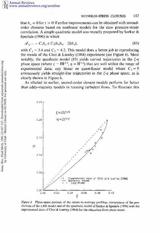
that bu = 0 for z > 0! Further improvements can be obtained with second-order closures based on nonlinear models for the slow pressure-straincorrelation. A simple quadratic model was recently proposed by Sarkar &Speziale (1990) in which
~u¢u = - C ~bu + C2( bikbk~-- ½II6u), (85)
with C~ = 3.4 and C2 - 4.2. This model does a better job in reproducingthe trends of the Choi & Lumley (1984) experiment (see Figure 6). notably, the quadratic model (85) yields curved trajectories in the {-r/phase space (where ~ = III 1/3, q = II ~/2) that are well within the range ofexperimental data; any linear or quasi-linear model where C2 = 0erroneously yields straight-line trajectories in the {-t/phase space, as isclearly shown in Figure 6.
As alluded to earlier, second-order closure models perform far betterthan eddy-viscosity models in rotating turbulent flows. To illustrate this
0.25
0.20
0.15
0.10
Qnd Lumley (1984)
0.000.00 0.02 0.04 0.06 0.08 O, 10
Figure 6 Phase-space portrait of the return-to-isotropy problem: comparison of the pre-dictions of the LRR model and of the quadratic model of Sarkar & Speziale (1990) with theexperimental data of Choi & Lumley (1984) for the relaxation from plane strain.
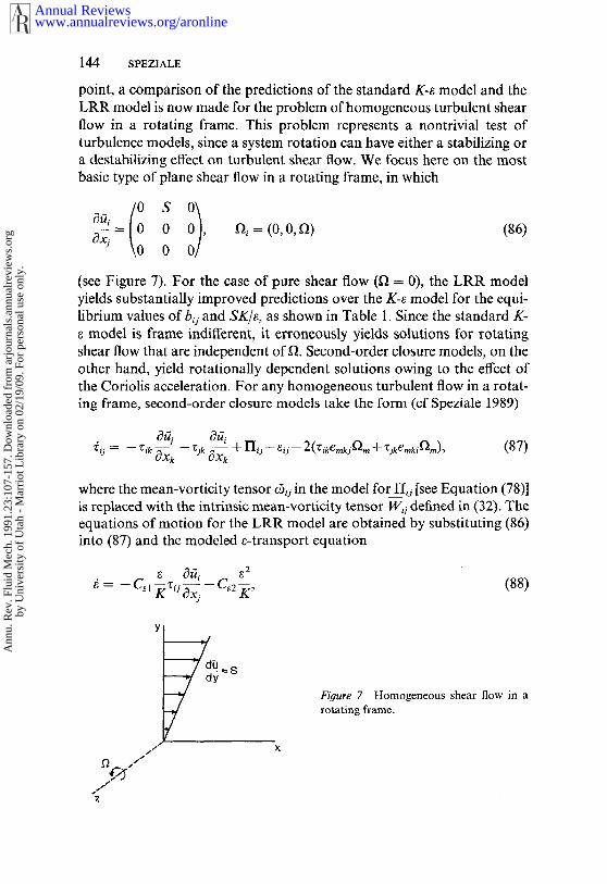
point, a comparison of the predictions of the standard K-e model and theLRR model is now made for the problem of homogeneous turbulent shearflow in a rotating frame. This problem represents a nontrivial test ofturbulence models, since a system rotation can have either a stabilizing ora destabilizing effect on turbulent shear flow. We focus here on the mostbasic type of plane shear flow in a rotating frame, in which
Ox~0 ,
0
~, = (0, 0, f~) (86)
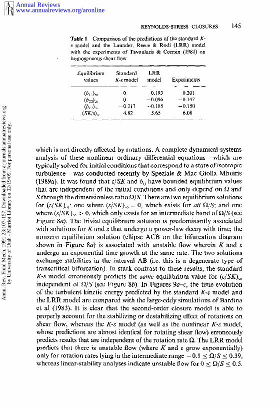
(see Figure 7). For the case of pure shear flow (f~ = 0), the LRR modelyields substantially improved predictions over the K-e model for the equi-librium values of bq and SK/e, as shown in Table 1. Since the standard K-e model is frame indifferent, it erroneously yields solutions for rotatingshear flow that are independent offL Second-order closure models, on theother hand, yield rotationally dependent solutions owing to the effect ofthe Coriolis acceleration. For any homogeneous turbulent flow in a rotat-ing frame, second-order closure models take the form (cf Speziale 1989)
where the mean-vorticity tensor ~q in the model for~q [see Equation (78)]is replaced with the intrinsic mean-vorticity tensor Wo defined in (32). Theequations of motion for the LRR model are obtained by substituting (86)into (87) and the modeled e-transport equation
(88)
Figure 7 Homogeneous shear flow in arotating frame.
Table 1 Comparison of the predictions of the standard K-e model and the Launder, Reece & Rodi (LRR) modelwith the experiments of Tavoularis & Corrsin (1980 onhomogeneous shear flow
Equilibrium Standard LRRvalues K-~ model model Experiments
which is not directly affected by rotations. A complete dynamical-systemsanalysis of these nonlinear ordinary differential equations--which aretypically solved for initial conditions that correspond to a state ofisotropicturbulence--was conducted recently by Speziale & Mac Giolla Mhuiris(1989a). It was found that e/SK and bij have bounded equilibrium valuesthat are independent of the initial conditions and only depend on f~ andS through the dimensionless ratio f~/S. There are two equilibrium solutionsfor (e/SK)~: one where (e/SK)® = O, which exists for all f~/S; and onewhere (e/SK)~ > 0, which only exists for an intermediate band of f~/S (seeFigure 8a). The trivial equilibrium solution is predominantly associatedwith solutions for K and e that undergo a power-law decay with time; thenonzero equilibrium solution (ellipse ACB on the bifurcation diagramshown in Figure 8a) is associated with unstable flow wherein K and undergo an exponential time growth at the same rate. The two solutionsexchange stabilities in the interval AB (i.e. this is a degenerate type oftranscritical bifurcation). In stark contrast to these results, the standardK-e model erroneously predicts the same equilibrium value for (~/SK)~independent of ~/S (see Figure 8b). In Figures 9a-c, the time evolutionof the turbulent kinetic energy predicted by the standard K-e model andthe LRR model are compared with the large-eddy simulations of Bardinaet al (1983). It is clear that the second-order closure model is able properly account for the stabilizing or destabilizing effect of rotations onshear flow, whereas the K-e model (as well as the nonlinear K-e model,whose predictions are almost identical for rotating shear flow) erroneouslypredicts results that are independent of the rotation rate f~. The LRR modelpredicts that there is unstable flow (where K and e grow exponentially)only for rotation rates lying in the intermediate range -0.1 < ~/S < 0.39,whereas linear-stability analyses indicate unstable flow for 0 < f~/S <_ 0.5.
Bifurcation diagram for rotating shear flow: (a) LRR model; (b) standard
Similar improved results using second-order closures have been recentlyobtained by Gatski & Savill (1989) for curved homogeneous shear flow.
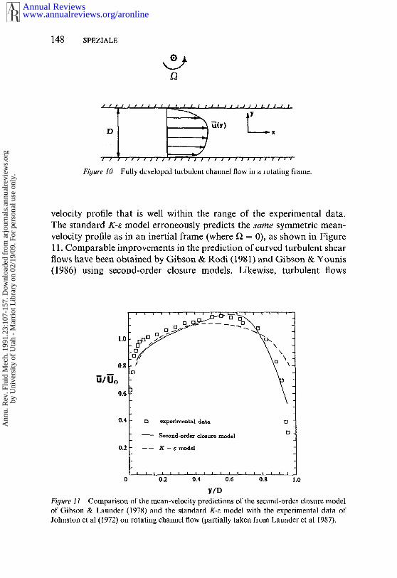
Finally, an example of an inhomogcneous wall-bounded turbulent flowis given. The problem of rotating channel flow recently considered byLaunder et al (1987) represents a challenging example. In this problem turbulent channel flow is subjected to a steady spanwisc rotation (seeFigure 10). Physical and numerical experiments (see Johnston et al 1972,Kim 1983) indicate that Coriolis forces arising from a system rotationcause the mean-velocity profile 5(y) to become asymmetric about the
Figure 9 Time evolution of the turbulent kinetic energy in rotating shear flow forzo/SKo = 0.296: (a) standard K-e model; (b) LRR model; and (c) large-eddy simulations(LES) of Bardina et al (1983).
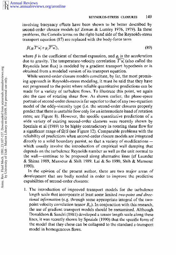
channel centerline. In Figure 11, the mean-velocity profile computed byLaunder et al (1987) using the Gibson & Launder (1978) second-orderclosure model is compared with the results of the K-~ model and theexperimental data of Johnston et al (1972) for a Reynolds numberRe = 11,500 and a rotation number Ro = 0.21. From this figure, it is clearthat the second-order closure model yields a highly asymmetric mean-
www.annualreviews.org/aronlineAnnual Reviews
Ann
u. R
ev. F
luid
Mec
h. 1
991.
23:1
07-1
57. D
ownl
oade
d fr
om a
rjou
rnal
s.an
nual
revi
ews.
org
by U
nive
rsity
of
Uta
h -
Mar
riot
Lib
rary
on
02/1
9/09
. For
per
sona
l use
onl
y.
148 SPEZIALE
Fiyure 10 Fully developed turbulent channel flow in a rotating frame.
velocity profile that is well within the range of the experimental data.The standard K-e model erroneously predicts the same symmetric mean-velocity profile as in an inertial frame (where ~ = 0), as shown in Figure11. Comparable improvements in the prediction of curved turbulent shearflows have been obtained by Gibson & Rodi (1981) and Gibson & Younis(1986) using second-order closure models. Likewise, turbulent flows
1.0
~/~o0.6
0.4
0.2
D experimental dat~ ~
~ Second-order clonure model El
---- K-¢model
0 0.2 0.4 0.6 0.8 1,0
¥/DFigure 11 Comparison of the mean-velocity predictions of the second-order closure modelof Gibson & Launder (1978) and the standard K-~, model with the experimental data Johnston et al (1972) on rotating channel flow (partially taken from Launder et al 1987).
involving buoyancy effects have been shown to be better described bysecond-order closure models (cf Zeman & Lumley 1976, 1979). In theseproblems, the Coriolis terms on the right-hand side of the Reynolds-stresstransport equation (87) are replaced with the body-force term
fl( giT’ uj + g jT’ u~), (89)
where fl is the coefficient of thermal expansion, and #i is the accelerationdue to gravity. The temperature-velocity correlation T’u~ (also called theReynolds heat flux) is modeled by a gradient transport hypothesis or isobtained from a modeled version of its transport equation.
While second-order closure models constitute, by far, the most promis-ing approach in Reynolds-stress modeling, it must be said that they havenot progressed to the point where reliable quantitative predictions can bemade for a variety of turbulent flows. To illustrate this point, we againcite the case of rotating shear flow. As shown earlier, the phase-spaceportrait of second-order closures is far superior to that of any two-equationmodel of the eddy-viscosity type (i.e. the second-order closures properlypredict that there is unstable flow only for an intermediate band of rotationrates; see Figure 8). However, the specific quantitative predictions of wide variety of existing second-order closures were recently shown bySpeziale et al (1989) to be highly contradictory in rotating shear flow fora significant range of f~/S (see Figure 12). Comparable problems with thereliability of predictions when second-order closure models are integrateddirectly to a solid boundary persist, so that a variety of modifications--which usually involve the introduction of empirical wall damping thatdepends on the turbulence Reynolds number as well as the unit normal tothe wall--continue to be proposed along alternative lines (cf Launder& Shima 1989, Mansour & Shih 1989, Lai & So 1990, Shih & Mansour1990).
In the opinion of the present author, there are two major areas ofdevelopment that are badly needed in order to improve the predictivecapabilities of second-order closures:
1. The introduction of improved transport models for the turbulencelength scale that ineorporate at least some limited two-point and direc-tional information (e.g. through some appropriate integral of the two-point velocity correlation tensor R~-). In conjunction with this research,the use of gradient transport models should be reexamined. AlthoughDonaldson & Sandri (1981) developed a tensor length scale along theselines, it was recently shown by Speziale (1990) that the specific form the model that they chose can be collapsed to the standard e-transportmodel in homogeneous flows.
Figure 12 Comparison of the predictions of a variety of secondiorder closure models
for the time evolution of the turbulent kinetic energy in rotating shear flow; ~/S = 0.25,eo/SKo = 0.296. LES --- large-eddy simulations of Bardina et al (1983); LRR ~ Launder,Reeee & Rodi model; RK--Rotta-Kolmogorov model of Meller & Herring (1973);FLT -- Fu, Launder & Tselepidakis (1987) model; RNG _= Renormalization Group modelof Yakhot & Orszag (1986); SL = Shih & Lumley (1985) model.
2. The need for asymptotically consistent low-turbulence-Reynolds-num-ber extensions of existing models that can be robustly integrated to asolid boundary. Existing models use ad hoc damping functions basedon Ret and have an implicit dependence on the unit normal to the wallthat does not allow for the proper treatment of geometrical dis-continuities such as those that occur in the square duct or back-stepproblems. Furthermore, the nonlinear effect of both rotational andirrotational strains need to be accounted for in the modeling of near-wall anisotropies in the dissipation.
In addition, the neglect of nonlocal and history effects in the commonlyadopted models (74)-(75) for the pressure-strain correlation needs to seriously reexamined. It has long been known that nonlocal effects can bequite important in strongly inhomogeneous turbulent flows. Furthermore,some inconsistencies that these algebraic models give rise to in rotatinghomogeneous turbulent flows have recently surfaced that appear to be dueto the neglect of history effects in the rapid pressure-strain terms (seeReynolds 1989, Speziale et al 1990).
There has been a tendency to be overly pessimistic about the progressmade in Reynolds-stress modeling during the past few decades. It must beremembered that the first complete Reynolds-stress models--cast in tensorform and supplemented only with initial and boundary conditions--weredeveloped less than 20 years ago. Progress was at first stymied by the lackof adequate computational power to properly explore full Reynolds-stressclosures in nontrivial turbulent flows--a deficiency that was not overcomeuntil the late 1960s. Then, by 1980--with an enormous increase in com-puter capacity efforts were shifted toward direct and large-eddy simu-lations of the Navier-Stokes equations. Furthermore, the interest in coher-ent structurcs (ef Hussain 1983) and in alternative theoretical approachesbased on nonlinear dynamics (e.g. period-doubling bifurcations as a routeto chaos; cf Swinney & Gollub 1981) that crystallized during the late 1970shas also diverted attention away from Reynolds-stress modeling, as wellas away from the general statistical approach for that matter. Whileprogress has been slow, this is due in large measure to the intrinsic com-plexity of the problem. The fact that real progress has been made, however,cannot be denied. Many of the turbulent flows considered in the lastsection--which were solved without the ad hoc adjustment of any con-stants--could not be properly analyzed by the Reynolds-stress modelsthat were available before 1970.
Some discussion is warranted concerning the goals and limitations ofReynolds-stress modeling. Under the best of circumstances, Reynolds-stress models can only provide accurate information about first and secondone-point moments (e.g. the mean velocity, mean pressure, and turbulenceintensity), which usually is all that is needed for design purposes. SinceReynolds-stress modeling constitutes a low-order one-point closure, itintrinsically cannot provide detailed information about flow structures.Furthermore, since spectral information needs to be indirectly built intoReynolds-stress models, a given model cannot bc cxpectcd to perform wellin a variety of turbulent flows where the spectrum of the energy-containingeddies is changing dramatically. However, to criticize Reynolds-stressmodels purely on the grounds that they are not based directly on solutionsof the full Navier-Stokes equations would be as simplistic as criticizingexact solutions of the Navier-Stokes equations for not being rigorouslyderived from the Boltzmann equation or, for that matter, from quantummechanics. The more appropriate question is whether or not a Reynolds-stress model can be developed that will provide adequate engineeringanswers for the mean velocity, mean pressure, and turbulence intensitiesin a significant range of turbulent flows that are of technological interest.
TO obtain accurate predictions for these quantities in all possible turbulentflows will probably require nothing short of solving the full Navier-Stokesequations. Such a task will not be achievable in the foreseeable future, ifever at all (cfHussaini et al 1990, Reynolds 1990). To gain an appreciationfor the magnitude of this task, consider the fact that economically feasibledirect simulations of turbulent pipe flow at a Reynolds number of500,000--a turbulent flow that, although nontrivial, is far from the mostdifficult encountered--would require a computer that is l0 million timesfaster than the Cray YMP!
While second-order closures represent the most promising approach inReynolds-stress modeling, much work remains to be done. The two prob-lem areas mentioned in the previous section--namely, the development oftransport models for an anisotropic integral length scale and the develop-ment of more asymptotically consistent methods for the integration ofsecond-order closures to a solid boundary--are of utmost importance. Infact, the issue of near-wall modeling is so crucial that deficiencies init along with associated numerical stiffness problems--are primarilyresponsible for the somewhat misleading critical evaluations of second-order closures that arose out of the 1980-81 AFOSR-HTTM-StanfordConference on Complex Turbulent Flows (see Kline et al 1981). Anotherarea that urgently needs attention is the second-order closure modeling ofcompressible turbulent flows. Until recently, most compressible second-order closure modeling has consisted of Favre-averaged, variable-densityextensions of the incompressible models (cf Cebeci & Smith 1974).However, with the current thrust in compressible second-order modelingat NASA Langley and NASA Ames, some new compressible modelingideas--such as dilatational dissipation--have come to the forefront (seeSarkar et al 1989, Zeman 1990). Much more work in this area is needed,however.
Reynolds-stress modeling should continue to steadily progress, comple-menting numerical simulations of the Navier-Stokes equations and alter-native theoretical approaches. In fact, with anticipated improvements incomputer capacity, direct numerical simulations should begin to play apivotal role in the screening and calibration of turbulence models. Therecent work on Reynolds-stress budgets at NASA Ames constitutes anexcellent example of this (see Mansour et al 1988). Furthermore, from thetheoretical side, statistical mechanics approaches such as RNG could beof considerable future use in the formulation of new models. (Unfor-tunately, at their current stage of development, it does not appear thatthey can reliably calibrate turbulence models for use in complex flows.)Although Reynolds-stress models provide information only about a lim-ited facet of turbulence, this information can have such important scientific
and engineering applications that these models are likely to remain a partof turbulence research for many years to come.
ACKNOWLEDGMENTS
The author would like to thank Drs. T. B. Gatski, N. Mac Giolla Mhuiris,and S. Sarkar for their assistance with some of the computations presentedin this paper. Helpful comments by Drs. M. Y. Hussaini, J. H. Ferziger,and J. L. Lumley are also gratefully acknowledged. This research wassupported under NASA Contract NAS1-18605 while the author was inresidence at ICASE.
Literature Cited
Avva, R. K., Kline, S. J., Ferziger, J. H.1988. Computation of the turbulent flowover a backward-facing step using thezonal modeling approach. Rep. No. TF-33, Stanford Univ., Stanford, Calif.
Baldwin, B. S., Lomax, H. 1978. Thin layerapproximation and algebraic model forseparated turbulent flows. AIAA Pap. No.78-257
Bardina, J., Ferziger, J. H., Reynolds, W. C.1983. Improved turbulence models basedon large-eddy simulation of homo-geneous, incompressible turbulent flows.Rep. No. TF-19, Stanford Univ., Stanford,Calif.
Bardina, J., Ferziger, J, H., Rogallo, R. S.1985. Effect of rotation on isotropic tur-bulence: computation and modeling. J.FluM Mech. 154:321-36
Bernard, P. S., Berger, B. S. 1982. A methodfor computing three-dimensional tur-bulent flows. SIAM J. Appl. Math. 42:453-70
Bertoglio, J. P. 1982. Homogeneous tur-bulent field within a rotating frame. AIAAJ. 20:1175-81
Boussinesq, J. 1877. Th6orie de l’6coulementtourbillant. M~rn. Pr~sent~s par diversSavants Acad. Sci. Inst. Ft. 23:46-50
Bradshaw, P., Ferriss, D. H., Atwell, N. P.1967. Calculation of boundary layer de-velopment using the turbulent energy equa-tion. J. Fluid Mech. 28:593-616
Bradshaw, P., Cebeci, T., Whitelaw, J. H.1981. Enyineerin9 Calculation Methods forTurbulent Flow. New York: Academic
Cebeci, T., Smith, A. M. O. 1968. A finite-difference solution of the incompressibleturbulent boundary-layer equations byan eddy viscosity concept. Proe. AROSR-IFP-Stanford Conf Comput. of Turbul.Boundary Layers, ed. S. J. Kline, M. V.
Morkovin, G. Sovran, D. S. Cockrell, 1:346-55. Stanford, Calif: Stanford Univ.Press
Cebeci, T., Smith, A. M. O. 1974. Analysisof Turbulent Boundary Layers. New York:Academic
Choi, K. S., Lumley, J. L. 1984. Return toisotropy of homogeneous turbulence re-visited. In Turbulence and Chaotic Phe-nomena in Fluids, ed. T. Tatsumi, pp. 267-72. New York: North-Holland
Clark, T. L., Farley, R. D. 1984. Severedownslope windstorm calculations in twoand three spatial dimensions using an-elastic interactive grid nesting: a possiblemechanism for gustiness. J. Atmos. Sci.41:329-50
Comte-Bellot, G., Corrsin, S. 1971. SimpleEulerian time correlation of full- and nar-row-band velocity signals in grid-gener-ated, "isotropic" turbulence. J. FluidMech. 48:273-337
Craft, T., Fu, S., Launder, B. E., Tsele-pidakis, D. P. 1989. Developments inmodeling the turbulent second-momentpressure correlations. Rep. No. TFD/89/1,Mech. Eng. Dep., Univ. Manchester Inst.Sci. Technol. Engl.
Crow, S. C. 1968. Viscoelastic properties offine-grained incompressible turbulence, J.Fluid Mech. 33:1-20
Daly, B. J., Harlow, F. H. 1970. Transportequations in turbulence. Phys. Fluids 13:2634-49
Deardorff, J. W. 1973. The use of subgridtransport equations in a three-dimen-sional model of atmospheric turbulence.ASME J. Fluids Eng. 95:429 38
Demuren, A., Rodi, W. 1984. Calculationof turbulence-driven secondary motion innon-circular ducts. J. Fluid Mech. 140:189-222
Donaldson, C. duP. 1972. Calculation of tur-bulent shear flows for atmospheric andvortex motions. AIAA J. 10:4-12
Donaldson, C. duP., Rosenbaum, H. 1968.Calculation of the turbulent shear flowsthrough closure of the Reynolds equationsby invariant modeling. Rep. No. 127,Aeronaut. Res. Assoc. Princeton, Prince-ton, N.J.
Donaldson, C. duP., Sandri, (3. 1981. On theinclusion of information on eddy structurein second-order closure model of tur-bulent flow. AGARD Rep. No. CP-308
Fu, S., Launder, B. E., Tselepidakis, D. P.1987. Accommodating the effects of highstrain rates in modelling the pressure-strain correlation. Rep. No. TFD/87/5,Mech. Eng. Dep., Univ. Manchester Inst.Sci. Technol., Engl.
Gatski, T. B., Savill, A. M. 1989. An analysisof curvature effects for the control of wall-bounded shear flows. AIAA Pap. No. 89-1014
Gessner, F. B., Po, J. K. 1976. A Reynoldsstress model for turbulent corner flow--Part II: comparisons between theory andexperiment. ASME J. Fluids Eng. 98: 269-77
Gibson, M. M., Launder, B. E. 1978. Groundeffects on pressure fluctuations in the at-mospheric boundary layer. J. Fluid Mech.86:491-511
Gibson, M. M., Rodi, W. 1981. A Reynoldsstress closure model of turbulence appliedto the calculation of a highly curved mix-ing layer. J. Fluid Mech. 103:161-82
Gibson, M. M., Younis, B. A. 1986. Cal-culation of swirling jets with a Reynoldsstress closure. Phys. Fluids 29:38-48
Hanjalib, K., Launder, B. E. 1972. A Rey-nolds stress model of turbulence and itsapplication to thin shear flows. J. FluidMech. 52:609 38
Hanjali6, K., Launder, B. E. 1976. Con-tribution towards a Reynolds stress clos-ure for low Reynolds number turbulence.J. Fluid Mech. 74:593-610
Hanjali6, K., Launder, B. E. 1980. Sen-sitizing the dissipation equation to irrota-tional strains. ASME J. Fluids Eng. 102:34-40
Haworth, D. C., Pope, S. B. 1986. A gener-alized Langevin model for turbulent flows.Phys. Fluids 29:387-405
Hinze, J. O. 1975. Turbulence. New York:Mc(3raw-Hill. 2nd ed.
Hussain, A. K. M. F. 1983. Coherent struc-tures: reality and myth. Phys. Fluids 26:2816-50
Hussaini, M. Y., Speziale, C. G., Zang, T.A. 1990. Discussion of the potential andlimitations of direct and large-eddy simu-lations. Proe. Whither Turbul. Workshop,
Johnson, D. A., King, L. S. 1984. A newturbulence closure model for boundarylayer flows with strong adverse pressuregradients and separation. AIAA Pap. No.84-0175
Johnston, J. P., Halteen, R. M., Lezius, D.K. 1972. Effects of a spanwise rotationon the structure of two-dimensional fully-developed turbulent channel flow. J. FluidMech. 56:533-57
Kim, J. 1983. The effect of rotation on tur-bulence structure. NASA TM-84379
Kim, J., Kline, S. J., Johnston, J. P. 1980.Investigation of a reattaching turbulentshear layer: flow over a backward-facingstep. ASME J. Fluids Eng. 102:302 8
Kline, S. J., Cantwell, B. J., Lilley, G. M.,eds. 1981. Proceedings of the 1980-81AFOSR-HTTM-Stanford Conference onComplex Turbulent Flows. Stanford, Calif:Stanford Univ. Press
Kolmogorov, A. N. 1942. The equations ofturbulent motion in an incompressiblefluid. Izv. Acad. Sci. USSR, Phys. 6: 56-58
Kraichnan, R. H. 1964. Direct interactionapproximation for shear and thermallydriven turbulence. Phys. Fluids 7:1048 62
Lai, Y. G., So, R. M. C. 1990. On near wallturbulent flow modeling. J. Fluid Mech.In press
Launder, B. E. 1990. Phenomenologicalinodeling: present and future. Proc. Whi-ther Turbul. Workshop, Ithaca, N.Y. LectNotes Phys., ed. J. L. Lumley, pp. 439-85.Berlin: Springer-Verlag
Launder, B. E., Reece, G. J., Rodi, W. 1975.Progress in the development of a Rey-nolds-stress turbulence closure. J. FluidMech. 68:537-66
Launder, B. E., Shima, N. 1989. Second-moment closure for the near-wall sub-layer: development and application. AIAAJ. 27:1319-23
Launder, B. E., Spalding, D. B. 1974. Thenumerical computation of turbulent flows.Comput. Methods Appl. Mech. Eng. 3:269-89
Launder, B. E., Tselepidakis, D. P., Younis,B. A. 1987. A second-moment closurestudy of rotating channel flow. J. FluidMech. 183:63-75
Launder, B. E., Ying, W. M. 1972. Second-ary flows in ducts of square cross-section.J. Fluid Mech. 54:289 95
Lesieur, M. 1987. Turbulence in Fluids. Bos-ton: Martinus Nijhoff
Lumley, J. L. 1970. Toward a turbulentconstitutive equation. J. Fluid Mech. 41:413-34
Lumley, J. L. 1978. Computational model-ing of turbulent flows. Adv. Appl. Mech.18:123-76
Lumley, J. L. 1983. Turbulence modeling.ASME J. Appl. Mech. 50:1097-1103
Lumley, J. L., Khajeh-Nouri, B. 1974. Com-putational modeling of turbulent trans-port. Adv. Geophys. 18A: 169-92
Mansour, N. N., Kim, J., Moin, P. 1988.Reynolds stress and dissipation rate bud-gets in turbulent channel flow. J. FluidMech. 194:15~44
Mansour, N. N., Shih, T. H. 1989. Advance-ments in turbulence modeling. In Forumon Turbulent Flows--1989, ed. W. W.Bower, M. J. Morris, FED-76: 129-41.New York: ASME
Mellor, G. L., Herring, H. J. 1973. A surveyof mean turbulent field closure models.AIAA J. 11:590-99
Mellor, G. L., Yamada, T. 1974. A hierarchyof turbulence closure models for planetaryboundary layers. J. Atmos. Sci. 31:17911806
Moin, P., Kim, J. 1982. Numerical inves-tigation of turbulent channel flow. J. FluidMech. 118:341-77
Nisizima, S., Yoshizawa, A, 1987. Turbu-lent channel and Couette flows using ananisotropic K-~ model. AIAA J. 25: 414-2O
Norris, L. H., Reynolds, W. C. 1975. Tur-bulent channel flow with a moving wavyboundary. Rep. No. FM-IO, StanfordUniv., Stanford, Calif.
Orszag, S. A. 1970. Analytical theories ofturbulence. J. Fluid Mech. 41:363-86
Patel, V. C., Rodi, W., Scheuerer, G. 1985.Turbulence models for near-wall and lowReynolds number flows: a review. AIAAJ. 23:1308-19
Piomelli, U., Ferziger, J. H., Moin, P. 1987.Models for large eddy simulations of tur-bulent channel flows including transpira-tion. Rep. No. TF-32, Stanford Univ., Stan-ford, Calif.
Pope, S. B. 1975. A more general effectiveviscosity hypothesis. J. Fluid Mech. 72:33140
Pope, S. B. 1978. An explanation of the tur-bulent round jet/plane jet anomaly. AIAAJ. 16:279-81
Pope, S. B. 1985. Pdf methods for turbulentreactive flows. Prog. Energy Combust. Sci.11:119-92
Prandtl, L. 1925. ~ber die ausgebildete Tur-bulenz. ZAMM 5:136-39
Prandtl, L. 1945. Ober ein neues Formel-system fiir die ausgebildete Turbulenz.Naehr. Akad. Wiss. G6ttingen, Math.-Phys. Kl. 1945:6-19
Reynolds, O. 1895. On the dynamical theoryof incompressible viscous fluids and the
REYNOLDS-STRESS CLOSURES 155determination of the criterion. Philos.Trans. R. Soc. London Set. A 186: 123-64
Reynolds, W. C. 1976. Computation of tur-bulent flows. Annu. Rev. Fluid Mech. 8:183-208
Reynolds, W. C. 1987. Fundamentals ofturbulence for turbulence modeling andsimulation. In Lecture Notes for Von Kf~r-m~n Institute. AGARD Lect. Ser. No. 86,pp. 1~6. New York: NATO
Reynolds, W. C. 1989. Effects of rotation onhomogeneous turbulence. Proc. Australas.Fluid Mech. Conf, lOth, pp. 1~5, Mel-bourne: Univ. Melbourne
Reynolds, W. C. 1990. The potential andlimitations of direct and large-eddy simu-lations. Proc. Whither Turbul. Workshop,Ithaca, N.Y. Lect. Notes Phys., ed. J.L. Lumley, pp. 313-42. Berlin: Springer-Verlag
Rivlin, R. S. 1957. The relation between theflow of non-Newtonian fluids and tur-bulent Newtonian fluids. Q. Appl. Math.15:212-15
Rodi, W. 1976. A new algebraic relation forcalculating the Reynolds stresses. ZAMM56:T219-21
Rodi, W. 1980. Turbulence Models and TheirApplication in HydrauBcs. Delft, Neth: lnt.Assoc. Hydraul. Res.
Rogallo, R. S., Moin, P. 1984. Numericalsimulation of turbulent flows. Annu. Rev.Fluid Mech. 16:99-137
Rotta, J. C. 1951. Statistische Theorie nich-thomogener Turbulenz. Z. Phys. 129: 547-72
Rotta, J. C. 1972. Recent attempts to de-velop a generally applicable calculationmethod for turbulent shear flow layers.AGARD CP-93
Rubinstein, R., Barton, J. M. 1990. Non-linear Reynolds stress models and the re-normalization group. Phys. Fluids A 2:1472-76
Saffman, P. G. 1977. Results of a two-equa-tion model for turbulent flows and de-velopment of a relaxation stress modelfor application to straining and rotatingflows. Proc. Proj. SQUID Workshop Tur-bul. in Intern. Flows, ed. S. Murthy, pp. 191-23 I. New York: Hemisphere
Sarkar, S., Erlebacher, G., Hussaini, M. Y.,Kreiss, H. O. 1989. The analysis and mod-eling of dilatational terms in compressibleturbulence. Rep. No. 89-79, ICASE, NASALangley Res. Cent., Hampton, Va.
Sarkar, S., Speziale, C. G. 1990. A simplenonlinear model for the return to isotropyin turbulence. Phys. Fluids A 2:84-93
Schlichting, H. 1968. Boundary Layer The-ory. New York: McGraw-Hill
Shih, T.-H., Lumley, J. L. 1985. Modelingof pressure correlation terms in Reynoldsstress and scalar flux equations. Rep.No. FDA-85-3, Cornell Univ., Ithaca,N.Y.
Shih, T.-H., Mansour, N. N. 1990. Second-order modeling of low Reynolds numberturbulence near walls. Submitted for pub-lication
Smagorinsky, J. 1963. General circulationexperiments with the primitive equations.Mon. Weather Rev. 91:99-165
Smith, G. F. 1971. On isotropic functions ofsymmetric tensors, skew-symmetric ten-sors and vectors. Int. J. Eng. Sci. 9: 899-916
Smolarkiewicz, P. K., Clark, T. L. 1985.Numerical simulation of a three-dimen-sional field of cumulus clouds. Part I.Model description, comparison with obser-vations and scnsitivity studies. J. Atmos.Sci. 42:502-22
Speziale, C. G. 1981. Some interesting prop-erties of two-dimensional turbulence.Phys. Fluids 24:142557
Speziale, C. G. 1983. Closure models forrotating two-dimensional turbulence.Geophys. Astrophys. Fluid Dyn. 23:6984
Speziale, C. G. 1985. Modeling the pressuregradient-velocity correlation of turbu-lence. Phys. Fluids 28:69-71
Speziale, C. G. 1987a. Second-order closuremodels for rotating turbulent flows. Q.Appl. Math. 45:721 33
Speziale, C. G. 1987b. On nonliltear K-l andK-e models of turbulence. J. Fluid Mech.178:459-75
Speziale, C. G. 1989. Turbulence modelingin non-inertial frames of reference. Theor.Comput. Fluid Dyn. 1:3 19
Speziale, C. G. 1990. Discussion of tur-bulence modeling: present and future. Proe.Whither Turbid. Workshop, Ithaca, N.Y.Leer. Notes Phys., ed. J. L. Lumley, pp.490-512. Berlin: Springer-Verlag
Speziale, C. G., Gatski, T. B., Mac GiollaMhuiris, N. 1989. A critical comparisonof turbulence models for homogeneousshear flows in a rotating frame. Proc.Syrup. Turbul. Shear Flows, 7th, 2: 27.3.1-27.3.6. Stanford, Calif: Stanford Uni-versity Press
Speziale, C. G., Mac Giolla Mhuiris, N.1989a. On the prediction of equilibriumstates in homogeneous turbulence. J. FluidMech. 209:591~15
Speziale, C. G., Mac Giolla Mhuiris, N.1989b. Scaling laws for homogeneous tur-bulent shear flows in a rotating frame.Phys. Fluids A 1:294-301
Speziale, C. G., Mansour, N. N., Rogallo,R. S. 1987. The decay of isotropic tur-bulence in a rapidly rotating frame. Proc.Summer Program Cent. for Turbul. Res.,ed. P. Moin, W. C. Reynolds, J. Kim, pp.205-11. Stanford, Calif: Stanford Univ.Press
Speziale, C. G., Ngo, T. 1988. Numericalsolution of turbulent flow past a back-ward-facing step using a nonlinear K-~model. Int. J. Eng. Sci. 26:1099-1112
Speziale, C. G., Sarkar, S., Gatski, T. B.1990. Modeling the pressure-strain cor-relation of turbulencc--an invariant dy-namical systems approach. Rep. No. 90-5, 1CASE, NASA Langley Res. Cent.,Hampton, Va.
Swinney, H. L., Gollub, J. P., eds. 1981.Hydrodynamic Instabilities and the Tran-sition to Turbulence. New York: Springer-Verlag
Tavoularis, S., Corrsin, S. 198 i. Experimentsin nearly homogeneous turbulent shearflow with a uniform mean temperaturegradient. Part I. J. Fluid Mech. 104:311-47
Taylor, G. I. 1915. Eddy motion in the atmo-sphere. Philos. Trans. R. Soc. London Set.A 215:1-26
Tennekes, H., Lumley, J. L. 1972. A FirstCourse in Turbulence. Cambridge, Mass:MIT Press. 300 pp.
von K~rm~.n, T. 1930. Mechanische /ihn-lichkeit und Turbulenz. Proc. Int. Congr.Appl. Mech., 3rd, Stockholm, Pt. 1, pp.85-105
von K~irm~n, T. 1948. Progress in the statis-tical theory of turbulence. Proc. Natl.Acad. Sei. USA 34:530-39
Weinstock, J. 1981. Theory of the pressure-strain rate correlation for Reynolds stressturbulence closures. Part 1. J. Fluid Mech.105:369-96
Wigeland, R. A., Nagib, H. M. 1978. Grid-generated turbulence with and withot~trotation about the streamwise direction.Rep. No. R78-1, I11. Inst. Technol., Chica-go
Wilcox, D. C. 1988. Reassessment of thescale-determining equation for advancedturbulence models. AIAA J. 26:12991310
Wilcox, D. C., Traci, R. M. 1976. A completemodel of turbulence. A1AA Pap. No. 76-351
Wolfshtein, M. 1970. On the length scale ofturbulence equation, lsr. J. Technol. 8: 87-99
Yakhot, V., Orszag, S. A. 1986. Renor-malization group analysis of turbulence.I. Basic theory. J. Sci. Comput. 1:3-51
Yoshizawa, A. 1984. Statistical analysis ofthe deviation of the Reynolds stress from
its eddy viscosity representation. Phys.Fluids 27:1377-87
Yoshizawa, A. 1987. Statistical modeling ofa transport equation for the kinetic energydissipation rate. Phys. Fluids 30:628-31
Zeman, O. 1990. Dilatation dissipation: theconcept and application in modeling com-prcssiblc mixing layers. Phys. Fluids A 2:178-88
REYNOLDS-STRESS CLOSURES 157Zeman, O., Lumley, J. L. 1976. Modeling
buoyancy-driven mixed layers. J. Atmos.Sci. 33:1974-88
Zeman, O., Lumley, J. L. 1979. Buoyancyeffects in entraining turbulent boundarylayers: a second-order closure study. InTurbulent Shear Flows I, ed. F. Durst, B.E. Launder, F. W. Schmidt, J. H. White-law, pp. 295-302. Berlin: Springer-Verlag