10.6 Variational Principle in Field Theory . . . . . . . . . . . . . . . . . . . . . . . . 50010.7 Appendix to linear PDEs discourse:
Symmetric Green’s Function of a real 2nd Order ODE . . . . . . . . . . . . . . 50310.8 Special Topic: Covariant Helmholtz Decomposition of 3-Vectors . . . . . . . . . 509
3
A Copyleft 512
B Group Theory 512
C Conventions 513
D Physical Constants and Dimensional Analysis 514
E Acknowledgments 517
F Last update: October 13, 2021 517
4
1 Preface
This work constitutes the free textbook project I initiated towards the end of Summer 2015,while preparing for the Fall 2015 Analytical Methods in Physics course I taught to upper level(mostly 2nd and 3rd year) undergraduates here at the University of Minnesota Duluth. DuringFall 2017, I taught the graduate-level Differential Geometry and Physics in Curved Spacetimeshere at National Central University, Taiwan; this has allowed me to further expand the text.
I assumed that the reader has taken the first three semesters of calculus, i.e., up to multi-variable calculus, as well as a first course in Linear Algebra and ordinary differential equations.(These are typical prerequisites for the Physics major within the US college curriculum.) Myprimary goal was to impart a good working knowledge of the mathematical tools that underliefundamental physics – quantum mechanics and electromagnetism, in particular. This meant thatLinear Algebra in its abstract formulation had to take a central role in these notes.1 To this end,I first reviewed complex numbers and matrix algebra. The middle chapters cover calculus beyondthe first three semesters: complex analysis and special/approximation/asymptotic methods. Thelatter, I feel, is not taught widely enough in the undergraduate setting. The final chapter is meantto give a solid introduction to the topic of linear partial differential equations (PDEs), whichis crucial to the study of electromagnetism, linearized gravitation and quantum mechanics/fieldtheory. But before tackling PDEs, I feel that having a good grounding in the basic elements ofdifferential geometry not only helps streamlines one’s fluency in multi-variable calculus; it alsoprovides a stepping stone to the discussion of curved spacetime wave equations.
Some of the other distinctive features of this free textbook project are as follows.Index notation and Einstein summation convention is widely used throughout the physics
literature, so I have not shied away from introducing it early on, starting in §(3) on matrixalgebra. In a similar spirit, I have phrased the abstract formulation of Linear Algebra in §(4)entirely in terms of P.A.M. Dirac’s bra-ket notation. When discussing inner products, I do makea brief comparison of Dirac’s notation against the one commonly found in math textbooks.
I made no pretense at making the material mathematically rigorous, but I strived to makethe flow coherent, so that the reader comes away with a firm conceptual grasp of the overallstructure of each major topic. For instance, while the full fledged study of continuous (as opposedto discrete) vector spaces can take up a whole math class of its own, I feel the physicist shouldbe exposed to it right after learning the discrete case. For, the basics are not only accessible, theFourier transform is in fact a physically important application of the continuous space spanned bythe position eigenkets |x⟩. One key difference between Hermitian operators in discrete versuscontinuous vector spaces is the need to impose appropriate boundary conditions in the latter;this is highlighted in the Linear Algebra chapter as a prelude to the PDE chapter §(10), wherethe Laplacian and its spectrum plays a significant role. Additionally, while the Linear Algebrachapter was heavily inspired by the first chapter of Sakurai’s Modern Quantum Mechanics, Ihave taken effort to emphasize that quantum mechanics is merely a very important applicationof the framework; for e.g., even the famous commutation relation [X i, Pj] = iδij is not necessarilya quantum mechanical statement. This emphasis is based on the belief that the power of a given
1That the textbook originally assigned for this course relegated the axioms of Linear Algebra towards thevery end of the discussion was one major reason why I decided to write these notes. This same book also costnearly two hundred (US) dollars – a fine example of exorbitant textbook prices these days – so I am glad I savedmy students quite a bit of their educational expenses that semester.
5
mathematical tool is very much tied to its versatility – this issue arises again in the JWKBdiscussion within §(6), where I highlight it is not merely some “semi-classical” limit of quantummechanical problems, but really a general technique for solving differential equations.
Much of §(5) is a standard introduction to calculus on the complex plane and the theoryof complex analytic functions. However, the Fourier transform application section gave methe chance to introduce the concept of the Green’s function; specifically, that of the ordinarydifferential equation describing the damped harmonic oscillator. This (retarded) Green’s functioncan be computed via the theory of residues – and through its key role in the initial valueformulation of the ODE solution, allows the two linearly independent solutions to the associatedhomogeneous equation to be obtained for any value of the damping parameter.
Differential geometry may appear to be an advanced topic to many, but it really is not.From a practical standpoint, it cannot be overemphasized that most vector calculus operationscan be readily carried out and the curved space(time) Laplacian/wave operator computed oncethe relevant metric is specified explicitly. I wrote much of §(8) in this “practical physicist”spirit. Although it deals primarily with curved spaces, teaching Physics in Curved Spacetimesduring Fall 2017 at National Central University, Taiwan, gave me the opportunity to add itscurved spacetime sequel, §(9), where I elaborated upon geometric concepts – the emergence ofthe Riemann tensor from parallel transporting a vector around an infinitesimal parallelogram,for instance – deliberately glossed over in §(8). It is my hope that §(8) and §(9) can be used tobuild the differential geometric tools one could then employ to understand General Relativity,Einstein’s field equations for gravitation.
In §(10) on PDEs, I begin with the Poisson equation in curved space, followed by the enu-meration of the eigensystem of the Laplacian in different flat spaces. By imposing Dirichlet orperiodic boundary conditions for the most part, I view the development there as the culminationof the Linear Algebra of continuous spaces. The spectrum of the Laplacian also finds importantapplications in the solution of the heat and wave equations. I have deliberately discussed theheat instead of the Schrodinger equation because the two are similar enough, I hope when thereader learns about the latter in her/his quantum mechanics course, it will only serve to en-rich her/his understanding when she/he compares it with the discourse here. Finally, the waveequation in Minkowski spacetime – the basis of electromagnetism and linearized gravitation – isdiscussed from both the position/real and Fourier/reciprocal space perspectives. The retardedGreen’s function plays a central role here, and I spend significant effort exploring different meansof computing it. The tail effect is also highlighted there: classical waves associated with masslessparticles transmit physical information within the null cone in (1 + 1)D and all odd dimensions.Wave solutions are examined from different perspectives: in real/position space; in frequencyspace; in the non-relativistic/static limits; and with the multipole-expansion employed to extractleading order features. The final section contains a brief introduction to the variational principlefor the classical field theories of the Poisson and wave equations.
Finally, I have interspersed problems throughout each chapter because this is how I personallylike to engage with new material – read and “doodle” along the way, to make sure I am properlyfollowing the details. My hope is that these notes are concise but accessible enough that anyonecan work through both the main text as well as the problems along the way; and discover theyhave indeed acquired a new set of mathematical tools to tackle physical problems.
By making this material available online, I view it as an ongoing project: I plan to updateand add new material whenever time permits; for instance, illustrations/figures accompanying
6
the main text may eventually show up at some point down the road. The most updated versioncan be found at the following URL:
2The motivational introduction to complex numbers, in particular the number i,3 is the solutionto the equation
i2 = −1. (2.0.1)
That is, “what’s the square root of −1?” For us, we will simply take eq. (2.0.1) as the definingequation for the algebra obeyed by i. A general complex number z can then be expressed as
z = x+ iy (2.0.2)
where x and y are real numbers. The x is called the real part (≡ Re(z)) and y the imaginarypart of z (≡ Im(z)).
Geometrically speaking z is a vector (x, y) on the 2-dimensional plane spanned by thereal axis (the x part of z) and the imaginary axis (the iy part of z). Moreover, you may recallfrom (perhaps) multi-variable calculus, that if r is the distance between the origin and the point(x, y) and ϕ is the angle between the vector joining (0, 0) to (x, y) and the positive horizontalaxis – then
(x, y) = (r cosϕ, r sinϕ). (2.0.3)
Therefore a complex number must be expressible as
z = x+ iy = r(cosϕ+ i sinϕ). (2.0.4)
This actually takes a compact form using the exponential:
z = x+ iy = r(cosϕ+ i sinϕ) = reiϕ, r ≥ 0, 0 ≤ ϕ < 2π. (2.0.5)
Some words on notation. The distance r between (0, 0) and (x, y) in the complex number contextis written as an absolute value, i.e.,
|z| = |x+ iy| = r =√x2 + y2, (2.0.6)
where the final equality follows from Pythagoras’ Theorem. The angle ϕ is denoted as
arg(z) = arg(reiϕ) = ϕ. (2.0.7)
The symbol C is often used to represent the 2D space of complex numbers.
z = |z|eiarg(z) ∈ C. (2.0.8)
Problem 2.1. Euler’s formula. Assuming exp z can be defined through its Taylor seriesfor any complex z, prove by Taylor expansion and eq. (2.0.1) that
eiϕ = cos(ϕ) + i sin(ϕ), ϕ ∈ R. (2.0.9)
2Some of the material in this section is based on James Nearing’s Mathematical Tools for Physics.3Engineers use j instead of i.
Arithmetic Addition and subtraction of complex numbers take place component-by-component, just like adding/subtracting 2D real vectors; for example, if
z1 = x1 + iy1 and z2 = x2 + iy2, (2.0.10)
then
z1 ± z2 = (x1 ± x2) + i(y1 ± y2). (2.0.11)
Multiplication is more easily done in polar coordinates: if z1 = r1eiϕ1 and z2 = r2e
iϕ2 , theirproduct amounts to adding their phases and multiplying their radii, namely
z1z2 = r1r2ei(ϕ1+ϕ2). (2.0.12)
To summarize:
Complex numbers z = x+iy = reiϕ|x, y ∈ R; r ≥ 0, ϕ ∈ R are 2D real vectors asfar as addition/subtraction goes – Cartesian coordinates are useful here (cf. (2.0.11)).It is their multiplication that the additional ingredient/algebra i2 ≡ −1 comes intoplay. In particular, using polar coordinates to multiply two complex numbers (cf.(2.0.12)) allows us to see the result is a combination of a re-scaling of their radii plusa rotation.
Problem 2.2. If z = x+ iy what is z2 in terms of x and y?
Problem 2.3. Explain why multiplying a complex number z = x + iy by i amounts torotating the vector (x, y) on the complex plane counter-clockwise by π/2. Hint: first write i inpolar coordinates.
Problem 2.4. Describe the points on the complex z-plane satisfying |z − z0| < R, wherez0 is some fixed complex number and R > 0 is a real number.
Problem 2.5. Use the polar form of the complex number to proof that multiplication ofcomplex numbers is associative, i.e., z1z2z3 = z1(z2z3) = (z1z2)z3.
Problem 2.6. Multiplication & Vector Calculus If z1 = x1 + iy1 and z2 = x2 + iy2,show that
z∗1z2 = z1 · z2 + i
([z10
]×[z20
])· e3. (2.0.13)
Here, we have converted the complex numbers into vectors via z1 ≡ (x1, y1)T and z2 ≡ (x2, y2)
T;whereas e3 ≡ (0, 0, 1)T.
Complex conjugation Taking the complex conjugate of z = x+ iy means we flip the signof its imaginary part, i.e.,
z∗ = x− iy; (2.0.14)
9
it is also denoted as z. In polar coordinates, if z = reiϕ = r(cosϕ + i sinϕ) then z∗ = re−iϕ
because
e−iϕ = cos(−ϕ) + i sin(−ϕ) = cosϕ− i sinϕ. (2.0.15)
The sinϕ→ − sinϕ is what brings us from x+ iy to x− iy. Now
When we take the ratio of complex numbers, it is possible to ensure that the imaginary numberi appears only in the numerator, by multiplying the numerator and denominator by the complexconjugate of the denominator. For x, y, a and b all real,
x+ iy
a+ ib=
(a− ib)(x+ iy)
a2 + b2=
(ax+ by) + i(ay − bx)
a2 + b2. (2.0.17)
Problem 2.7. Is (z1z2)∗ = z∗1z
∗2 , i.e., is the complex conjugate of the product of 2 complex
numbers equal to the product of their complex conjugates? What about (z1/z2)∗ = z∗1/z
∗2? Is
|z1z2| = |z1||z2|? What about |z1/z2| = |z1|/|z2|? Also show that arg(z1 · z2) = arg(z1)+ arg(z2).Strictly speaking, arg(z) is well defined only up to an additive multiple of 2π. Can you explainwhy? Hint: polar coordinates are very useful in this problem.
Problem 2.8. Show that z is real if and only if z = z∗. Show that z is purely imaginaryif and only if z = −z∗. Show that z + z∗ = 2Re(z) and z − z∗ = 2iIm(z). Hint: use Cartesiancoordinates.
Problem 2.9. Prove that the roots of a polynomial with real coefficients
PN(z) ≡ c0 + c1z + c2z2 + · · ·+ cNz
N , ci ∈ R, (2.0.18)
come in complex conjugate pairs; i.e., if z is a root then so is z∗.
Trigonometric, hyperbolic and exponential functions Complex numbers allow us toconnect trigonometric, hyperbolic and exponential (exp) functions. Start from
e±iϕ = cosϕ± i sinϕ. (2.0.19)
These two equations can be added and subtracted to yield
cos(z) =eiz + e−iz
2, sin(z) =
eiz − e−iz
2i, tan(z) =
sin(z)
cos(z). (2.0.20)
We have made the replacement ϕ → z. This change is cosmetic if 0 ≤ z < 2π, but we can infact now use eq. (2.0.20) to define the trigonometric functions in terms of the exp function forany complex z.
Trigonometric identities can be readily obtained from their exponential definitions. Forexample, the addition formulas would now begin from
ei(θ1+θ2) = eiθ1eiθ2 . (2.0.21)
10
Applying Euler’s formula (eq. (2.0.9)) on both sides,
cos(θ1 + θ2) + i sin(θ1 + θ2) = (cos θ1 + i sin θ1)(cos θ2 + i sin θ2) (2.0.22)
= (cos θ1 cos θ2 − sin θ1 sin θ2) + i(sin θ1 cos θ2 + sin θ2 cos θ1).
If we suppose θ1,2 are real angles, equating the real and imaginary parts of the left-hand-sideand the last line tell us
cos(θ1 + θ2) = cos θ1 cos θ2 − sin θ1 sin θ2, (2.0.23)
sin(θ1 + θ2) = sin θ1 cos θ2 + sin θ2 cos θ1. (2.0.24)
Problem 2.10. You are probably familiar with the hyperbolic functions, now defined as
cosh(z) =ez + e−z
2, sinh(z) =
ez − e−z
2, tanh(z) =
sinh(z)
cosh(z), (2.0.25)
for any complex z. Show that
cosh(iz) = cos(z), sinh(iz) = i sin(z), cos(iz) = cosh(z), sin(iz) = i sinh(z). (2.0.26)
Problem 2.11. Calculate, for real θ and positive integer N :
Hint: consider the geometric series eiθ + e2iθ + · · ·+ eNiθ.
Problem 2.12. Starting from (eiθ)n, for arbitrary integer n, re-write cos(nθ) and sin(nθ)as a sum involving products/powers of sin θ and cos θ. Hint: if the arbitrary n case is confusingat first, start with n = 1, 2, 3 first.
Roots of unity In polar coordinates, circling the origin n times bring us back to thesame point,
z = reiθ+i2πn, n = 0,±1,±2,±3, . . . . (2.0.29)
This observation is useful for the following problem: what is mth root of 1, when m is a positiveinteger? Of course, 1 is an answer, but so are
11/m = ei2πn/m, n = 0, 1, . . . ,m− 1. (2.0.30)
The terms repeat themselves for n ≥ m; the negative integers n do not give new solutions for minteger. If we replace 1/m with a/b where a and b are integers that do not share any commonfactors, then
1a/b = ei2πn(a/b) for n = 0, 1, . . . , b− 1, (2.0.31)
11
since when n = b we will get back 1. If we replaced (a/b) with say 1/π,
11/π = ei2πn/π = ei2n, (2.0.32)
then there will be infinite number of solutions, because 1/π cannot be expressed as a ratio ofintegers – there is no way to get 2n = 2πn′, for n′ integer.
In general, when you are finding the mth root of a complex number z, you are actuallysolving for w in the polynomial equation wm = z. The fundamental theorem of algebra tells us,if m is a positive integer, you are guaranteed m solutions – although not all of them may bedistinct.
Square root of −1 What is√−1? Since −1 = ei(π+2πn) for any integer n,
(ei(π+2πn))1/2 = eiπ/2+iπn = ±i. n = 0, 1. (2.0.33)
Problem 2.13. Find all the solutions to√1− i.
Logarithm and powers As we have just seen, whenever we take the root of somecomplex number z, we really have a multi-valued function. The inverse of the exponential isanother such function. For w = x+ iy, where x and y are real, we may consider
ew = exei(y+2πn), n = 0,±1,±2,±3, . . . . (2.0.34)
We define ln to be such that
ln ew = x+ i(y + 2πn). (2.0.35)
Another way of saying this is, for a general complex z,
ln(z) = ln |z|+ i(arg(z) + 2πn). (2.0.36)
One way to make sense of how to raise a complex number z = reiθ to the power of anothercomplex number w = x+ iy, namely zw, is through the ln:
zw = ew ln z = e(x+iy)(ln(r)+i(θ+2πn)) = ex ln r−y(θ+2πn)ei(y ln(r)+x(θ+2πn)). (2.0.37)
This is, of course, a multi-valued function. We will have more to say about such multi-valuedfunctions when discussing their calculus in §(5).
Problem 2.14. Find the inverse hyperbolic functions of eq. (2.0.25) in terms of ln. Doessin(z) = 0, cos(z) = 0 and tan(z) = 0 have any complex solutions? Hint: for the first question,write ez = w and e−z = 1/w. Then solve for w. A similar strategy may be employed for thesecond question.
Problem 2.15. Let ξ and ξ′ be vectors in a 2D Euclidean space, i.e., you may assume theirCartesian components are
Use complex numbers, and assume that the following complex Taylor expansion of ln holds
ln(1− z) = −∞∑ℓ=1
zℓ
ℓ, |z| < 1, (2.0.39)
to show that
ln |ξ − ξ′| = ln r> −∞∑ℓ=1
1
ℓ
(r<r>
)ℓ
cos(ℓ(ϕ− ϕ′)
), (2.0.40)
where r> is the larger and r< is the smaller of the (r, r′), and |ξ− ξ′| is the distance between the
vectors ξ and ξ′ – not the absolute value of some complex number. Here, ln |ξ− ξ′| is proportionalto the electric or gravitational potential generated by a point charge/mass in 2-dimensional flatspace. Hint: first let z = reiϕ and z′ = r′eiϕ
′; then consider ln(z − z′) – how do you extract
ln |ξ − ξ′| from it?
13
3 Matrix Algebra
4In this section I will review some basic properties of matrices and matrix algebra, oftentimesusing index notation. We will assume all matrices have complex entries unless otherwise stated.This is primarily intended to be warmup to the next section, where I will treat Linear Algebrafrom a more abstract point of view.
3.1 Basics, Matrix Operations, and Special types of matrices
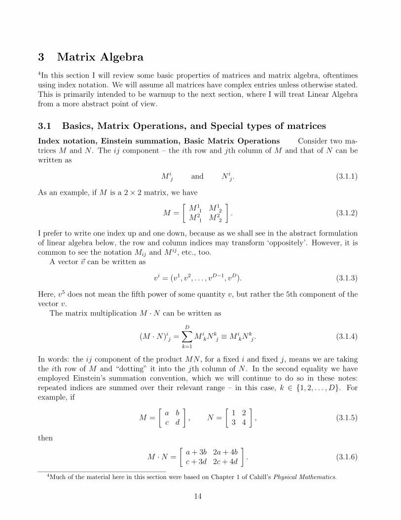
Index notation, Einstein summation, Basic Matrix Operations Consider two ma-trices M and N . The ij component – the ith row and jth column of M and that of N can bewritten as
M ij and N i
j. (3.1.1)
As an example, if M is a 2× 2 matrix, we have
M =
[M1
1 M12
M21 M2
2
]. (3.1.2)
I prefer to write one index up and one down, because as we shall see in the abstract formulationof linear algebra below, the row and column indices may transform ‘oppositely’. However, it iscommon to see the notation Mij and M
ij, etc., too.A vector v can be written as
vi = (v1, v2, . . . , vD−1, vD). (3.1.3)
Here, v5 does not mean the fifth power of some quantity v, but rather the 5th component of thevector v.
The matrix multiplication M ·N can be written as
(M ·N)ij =D∑
k=1
M ikN
kj ≡M i
kNkj. (3.1.4)
In words: the ij component of the product MN , for a fixed i and fixed j, means we are takingthe ith row of M and “dotting” it into the jth column of N . In the second equality we haveemployed Einstein’s summation convention, which we will continue to do so in these notes:repeated indices are summed over their relevant range – in this case, k ∈ 1, 2, . . . , D. Forexample, if
M =
[a bc d
], N =
[1 23 4
], (3.1.5)
then
M ·N =
[a+ 3b 2a+ 4bc+ 3d 2c+ 4d
]. (3.1.6)
4Much of the material here in this section were based on Chapter 1 of Cahill’s Physical Mathematics.
14
Note: M ikN
kj works for multiplication of non-square matrices M and N too, as long as the
number of columns ofM is equal to the number of rows of N , so that the sum involving k makessense.
Addition of M and N ; and multiplication of M by a complex number λ goes respectively as
(M +N)ij =M ij +N i
j (3.1.7)
and
(λM)ij = λM ij. (3.1.8)
Associativity The associativity of matrix multiplication means (AB)C = A(BC) = ABC.This can be seen using index notation
AikB
klC
lj = (AB)ilC
lj = Ai
k(BC)kj = (ABC)ij. (3.1.9)
Tr Tr(A) ≡ Aii denotes the trace of a square matrix A. The index notation makes it clear
the trace of AB is that of BA because
Tr [A ·B] = AlkB
kl = Bk
lAlk = Tr [B · A] . (3.1.10)
This immediately implies the Tr is cyclic, in the sense that
Comment on whether it makes sense to define Tr(A) ≡ Aii, if A is not a square matrix.
Identity and the Kronecker delta The D ×D identity matrix I has 1 on each andevery component on its diagonal and 0 everywhere else. This is also the Kronecker delta.
Iij = δij = 1, i = j
= 0, i = j (3.1.13)
The Kronecker delta is also the flat Euclidean metric in D spatial dimensions; in that contextwe would write it with both lower indices δij and its inverse is δij.
The Kronecker delta is also useful for representing diagonal matrices. These are matrices thathave non-zero entries strictly on their diagonal, where row equals to column number. For exampleAi
j = aiδij = ajδ
ij is the diagonal matrix with a1, a2, . . . , aD filling its diagonal components, from
the upper left to the lower right. Diagonal matrices are also often denoted, for instance, as
A = diag[a1, . . . , aD]. (3.1.14)
Suppose we multiply AB, where B is also diagonal (Bij = biδ
ij = bjδ
ij),
(AB)ij =∑l
aiδilbjδ
lj. (3.1.15)
15
If i = j there will be no l that is simultaneously equal to i and j; therefore either one or boththe Kronecker deltas are zero and the entire sum is zero. If i = j then when (and only when)l = i = j, the Kronecker deltas are both one, and
(AB)ij = aibj. (3.1.16)
This means we have shown, using index notation, that the product of diagonal matrices yieldsanother diagonal matrix.
(AB)ij = aibjδij (No sum over i, j). (3.1.17)
Transpose The transpose T of any matrix A is
(AT)ij = Aji. (3.1.18)
In words: the i row of AT is the ith column of A; the jth column of AT is the jth row of A. IfA is a (square) D ×D matrix, you reflect it along the diagonal to obtain AT.
Problem 3.2. Show using index notation that (A ·B)T = BTAT.
Adjoint The adjoint † of any matrix is given by
(A†)ij = (Aji)∗ = (A∗)ji. (3.1.19)
In other words, A† = (AT)∗; to get A†, you start with A, take its transpose, then take its complexconjugate. An example is,
A =
[1 + i eiθ
x+ iy√10
], 0 ≤ θ < 2π, x, y ∈ R (3.1.20)
AT =
[1 + i x+ iy
eiθ√10
], A† =
[1− i x− iy
e−iθ√10
]. (3.1.21)
Orthogonal, Unitary, Symmetric, and Hermitian A D ×D matrix A is
1. Orthogonal if ATA = AAT = I. The set of real orthogonal matrices implement rotationsin a D-dimensional real (vector) space.
2. Unitary if A†A = AA† = I. Thus, a real unitary matrix is orthogonal. Moreover, unitarymatrices, like their real orthogonal counterparts, implement “rotations” in aD dimensionalcomplex (vector) space.
3. Symmetric if AT = A; anti-symmetric if AT = −A.
4. Hermitian if A† = A; anti-hermitian if A† = −A.
Problem 3.3. Explain why, if A is an orthogonal matrix, it obeys the equation
AikA
jlδij = δkl. (3.1.22)
Now explain why, if A is a unitary matrix, it obeys the equation
(Aik)
∗Ajlδij = δkl. (3.1.23)
16
Problem 3.4. Prove that (AB)T = BTAT and (AB)† = B†A†. This means if A and B areorthogonal, then AB is orthogonal; and if A and B are unitary AB is unitary. Can you explainwhy?
Simple examples of a unitary, symmetric and Hermitian matrix are, respectively (from left toright): [
eiθ 00 eiδ
],
[eiθ XX eiδ
],
[ √109 1− i
1 + i θδ
], θ, δ ∈ R. (3.1.24)
3.2 Determinants, Linear (In)dependence, Inverses, Eigensystems
Levi-Civita symbol and the Determinant We will now define the determinant of aD × D matrix A through the Levi-Civita symbol ϵi1i2...iD−1iD , where every index runs from 1through D:
detA ≡ ϵi1i2...iD−1iDAi11A
i22 . . . A
iD−1
D−1AiD
D. (3.2.1)
This definition is equivalent to the usual co-factor expansion definition.The D−dimensional Levi-Civita symbol is defined through the following properties.
It is completely antisymmetric in its indices. This means swapping any of the indicesia ↔ ib (for a = b) will return
In matrix algebra and flat Euclidean space, ϵ123...D = ϵ123...D ≡ 1.5
These are sufficient to define every component of the Levi-Civita symbol. Because ϵ is fully anti-symmetric, if any of its D indices are the same, say ia = ib, then the Levi-Civita symbol returnszero. (Why?) Whenever i1 . . . iD are distinct indices, ϵi1i2...iD−1iD is really the sign of the per-mutation (≡ (−)nunber of swaps of index pairs) that brings 1, 2, . . . , D− 1, D to i1, i2, . . . , iD−1, iD.Hence, ϵi1i2...iD−1iD is +1 when it takes zero/even number of swaps, and −1 when it takes odd.
For example, in the 2 dimensional case ϵ11 = ϵ22 = 0; whereas it takes one swap to go from12 to 21. Therefore,
5In Lorentzian flat spacetimes, the Levi-Civita tensor with upper indices will need to be carefully distinguishedfrom its counterpart with lower indices.
17
for all square matrices A and B. As a simple example, let us use eq. (3.2.1) to calculate thedeterminant of
A =
[a bc d
]. (3.2.6)
Remember the only non-zero components of ϵi1i2 are ϵ12 = 1 and ϵ21 = −1.
detA = ϵ12A11A
22 + ϵ21A
21A
12 = A1
1A22 − A2
1A12
= ad− bc. (3.2.7)
Problem 3.5. Inverse of 2 × 2 matrix By viewing ϵ as a 2 × 2 matrix, prove that,whenever the inverse of a matrix M exist, it can be written as
M−1 = −ϵ ·MT · ϵ
detM=ϵ† ·MT · ϵdetM
=ϵ ·MT · ϵ†
detM. (3.2.8)
Hint: Can you explain why eq. (3.2.1) implies
ϵABMAIM
BJ = ϵIJ detM? (3.2.9)
Then contract both sides with M−1 and use ϵ2 = −I. Or, simply prove it by brute force.
Problem 3.6. Explain why eq. (3.2.1) implies
ϵi1i2...iD−1iDAi1j1Ai2
j2. . . A
iD−1
jD−1AiD
jD= ϵj1j2...jD−1jD detA. (3.2.10)
Hint: What happens when you swap Aimm and Ain
n in eq. (3.2.1)?
Linear (in)dependence Given a set of D vectors v1, . . . , vD, we say one of them islinearly dependent (say vi) if we can express it in as a sum of multiples of the rest of the vectors,
vi =D−1∑j =i
χjvj for some χj ∈ C. (3.2.11)
We say the D vectors are linearly independent if none of the vectors are linearly dependent onthe rest.
Det as test of linear independence If we view the columns or rows of a D × D matrixA as vectors and if these D vectors are linearly dependent, then the determinant of A is zero.This is because of the antisymmetric nature of the Levi-Civita symbol. Moreover, supposedetA = 0. Cramer’s rule (cf. eq. (3.2.24) below) tells us the inverse A−1 exists. In fact, forfinite dimensional matrix A, its inverse A−1 is unique. That means the only solution to theD-component row (or column) vector w, obeying w ·A = 0 (or, A ·w = 0), is w = 0. And sincew · A (or A · w) describes the linear combination of the rows (or, columns) of A; this indicatesthey must be linearly independent whenever detA = 0.
For a square matrix A, detA = 0 iff (≡ if and only if) its columns and rowsare linearly dependent. Equivalently, detA = 0 iff its columns and rows are linearlyindependent.
18
Problem 3.7. If the columns of a square matrix A are linearly dependent, use eq. (3.2.1)to prove that detA = 0. Hint: use the antisymmetric nature of the Levi-Civita symbol.
Problem 3.8. Show that, for a D ×D matrix A and some complex number λ,
det(λA) = λD detA. (3.2.12)
Hint: this follows almost directly from eq. (3.2.1).Relation to cofactor expansion The co-factor expansion definition of the determinant
is
detA =D∑i=1
AikC
ik, (3.2.13)
where k is an arbitrary integer from 1 through D. The Cik is (−)i+k times the determinant of
the (D − 1) × (D − 1) matrix formed from removing the ith row and kth column of A. (Thisdefinition sums over the row numbers; it is actually equally valid to define it as a sum overcolumn numbers.)
As a 3× 3 example, we have
det
a b cd e fg h l
= b(−)1+2 det
[d fg l
]+ e(−)2+2 det
[a cg l
]+ h(−)3+2 det
[a cd f
].
(3.2.14)
Pauli Matrices The 2×2 identity together with the Pauli matrices are Hermitian matrices.
σ0 ≡[1 00 1
], σ1 ≡
[0 11 0
], σ2 ≡
[0 −ii 0
], σ3 ≡
[1 00 −1
](3.2.15)
Problem 3.9. Let pµ ≡ (p0, p1, p2, p3) be a 4-component collection of complex numbers.Verify the following determinant, relevant for the study of Lorentz symmetry in 4-dimensionalflat spacetime,
det pµσµ =
∑0≤µ,ν≤3
ηµνpµpν ≡ p2, (3.2.16)
where pµσµ ≡
∑0≤µ≤3 pµσ
µ and
ηµν ≡
1 0 0 00 −1 0 00 0 −1 00 0 0 −1
. (3.2.17)
(This is the metric in 4 dimensional flat “Minkowski” spacetime.) Verify, for i, j, k ∈ 1, 2, 3and ϵ denoting the 2D Levi-Civita symbol,
detσ0 = 1, detσi = −1, Tr[σ0]= 2, Tr
[σi]= 0 (3.2.18)
σiσj = δijI+ i∑
1≤k≤3
ϵijkσk, ϵσiϵ = (σi)∗ = ϵ(−σi)ϵ†. (3.2.19)
19
Also use the antisymmetric nature of the Levi-Civita symbol to aruge that
θiθjϵijk = 0. (3.2.20)
Use these facts to derive the result:
U(θ) ≡ exp
[− i
2
3∑j=1
θjσj
]≡ e−(i/2)θ·σ
= cos
(1
2|θ|)− i
θ · σ|θ|
sin
(1
2|θ|), |θ| =
√θiθi ≡
√θ · θ, (3.2.21)
which is valid for complex θi. (Hint: Taylor expand expX =∑∞
ℓ=0Xℓ/ℓ!, followed by applying
the first relation in eq. (3.2.19).)Show that any 2 × 2 complex matrix A can be built from pµσ
µ by choosing the pµs appro-priately. Then compute (1/2)Tr [pµσ
µσν ], for ν = 0, 1, 2, 3, and comment on how the trace canbe used, given A, to solve for the pµ in the equation
pµσµ = A. (3.2.22)
Inverse The inverse of the D ×D matrix A is defined to be
A−1A = AA−1 = I. (3.2.23)
The inverse A−1 of a finite dimensional matrix A is unique; moreover, the left A−1A = I andright inverses AA−1 = I are the same object. The inverse exists if and only if (≡ iff) detA = 0.
Problem 3.10. Cramer’s rule Can you show the equivalence of equations (3.2.1) and(3.2.13)? Can you also show that
δkl detA =D∑i=1
AikC
il? (3.2.24)
That is, show that when k = l, the sum on the right hand side is zero. Explain why eq. (3.2.24)informs us that
(A−1)li = (detA)−1
D∑i=1
Cil. (3.2.25)
Hint: start from the left-hand-side, namely
detA = ϵj1...jDAj11 . . . A
jDD (3.2.26)
= Aik
(ϵj1...jk−1ijk+1...jDA
j11 . . . A
jk−1
k−1Ajk+1
k+1 . . . AjD
D
),
where k is an arbitrary integer in the set 1, 2, 3, . . . , D − 1, D. Examine the term in theparenthesis. First shift the index i, which is located at the kth slot from the left, to the ithslot. Then argue why the result is (−)i+k times the determinant of A with the ith row and kthcolumn removed. Finally, remember A−1 · A = I.
20
Problem 3.11. Why are the left and right inverses of (an invertible) matrix A the same?Hint: Consider LA = I and AR = I; for the first, multiply R on both sides from the right.
Problem 3.12. Prove that (A−1)T = (AT)−1 and (A−1)† = (A†)−1.
Eigenvectors and Eigenvalues If A is a D × D matrix, v is its (D-component)eigenvector with eigenvalue λ if it obeys
Aijv
j = λvi. (3.2.27)
This means
(Aij − λδij)v
j = 0 (3.2.28)
has non-trivial solutions iff
PD(λ) ≡ det (A− λI) = 0. (3.2.29)
Equation (3.2.29) is known as the characteristic equation. For a D × D matrix, it gives us aDth degree polynomial PD(λ) for λ, whose roots are the eigenvalues of the matrix λ – the setof all eigenvalues of a matrix is called its spectrum. For each solution for λ, we then proceed tosolve for the vi in eq. (3.2.28). That there is always at least one solution – there could be more– for vi is because, since its determinant is zero, the columns of A − λI are necessarily linearlydependent. As already discussed above, this amounts to the statement that there is some sum ofmultiples of these columns (≡ “linear combination”) that yields zero – in fact, the componentsof vi are precisely the coefficients in this sum. If wi are these columns of A− λI,
A− λI ≡ [w1w2 . . . wD] ⇒ (A− λI)v =∑j
wjvj = 0. (3.2.30)
(Note that, if∑
j wjvj = 0 then
∑j wj(Kv
j) = 0 too, for any complex numberK; in other words,eigenvectors are only defined up to an overall multiplicative constant.) Every D×D matrix hasD eigenvalues from solving the Dth order polynomial equation (3.2.29); from that, you can thenobtain D corresponding eigenvectors. Note, however, the eigenvalues can be repeated; when thisoccurs, it is known as a degenerate spectrum. Moreover, not all the eigenvectors are guaranteedto be linearly independent; i.e., some eigenvectors can turn out to be sums of multiples of othereigenvectors.
The Cayley-Hamilton theorem states that the matrix A satisfies its own characteristicequation. In detail, if we express eq. (3.2.29) as
∑Di=0 qiλ
i = 0 (for appropriate complex constantsqi), then replace λi → Ai (namely, the ith power of λ with the ith power of A), we would find
PD(A) = 0. (3.2.31)
Any D×D matrix A admits a Schur decomposition. Specifically, there is some unitary matrixU such that A can be brought to an upper triangular form, with its eigenvalues on the diagonal:
U †AU = diag(λ1, . . . , λD) +N, (3.2.32)
21
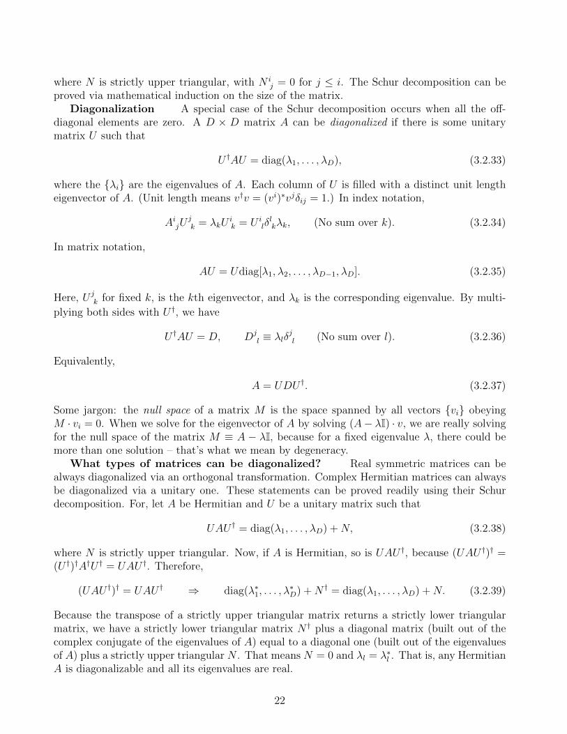
where N is strictly upper triangular, with N ij = 0 for j ≤ i. The Schur decomposition can be
proved via mathematical induction on the size of the matrix.Diagonalization A special case of the Schur decomposition occurs when all the off-
diagonal elements are zero. A D × D matrix A can be diagonalized if there is some unitarymatrix U such that
U †AU = diag(λ1, . . . , λD), (3.2.33)
where the λi are the eigenvalues of A. Each column of U is filled with a distinct unit lengtheigenvector of A. (Unit length means v†v = (vi)∗vjδij = 1.) In index notation,
AijU
jk = λkU
ik = U i
lδlkλk, (No sum over k). (3.2.34)
In matrix notation,
AU = Udiag[λ1, λ2, . . . , λD−1, λD]. (3.2.35)
Here, U jk for fixed k, is the kth eigenvector, and λk is the corresponding eigenvalue. By multi-
plying both sides with U †, we have
U †AU = D, Djl ≡ λlδ
jl (No sum over l). (3.2.36)
Equivalently,
A = UDU †. (3.2.37)
Some jargon: the null space of a matrix M is the space spanned by all vectors vi obeyingM · vi = 0. When we solve for the eigenvector of A by solving (A− λI) · v, we are really solvingfor the null space of the matrix M ≡ A − λI, because for a fixed eigenvalue λ, there could bemore than one solution – that’s what we mean by degeneracy.
What types of matrices can be diagonalized? Real symmetric matrices can bealways diagonalized via an orthogonal transformation. Complex Hermitian matrices can alwaysbe diagonalized via a unitary one. These statements can be proved readily using their Schurdecomposition. For, let A be Hermitian and U be a unitary matrix such that
UAU † = diag(λ1, . . . , λD) +N, (3.2.38)
where N is strictly upper triangular. Now, if A is Hermitian, so is UAU †, because (UAU †)† =(U †)†A†U † = UAU †. Therefore,
Because the transpose of a strictly upper triangular matrix returns a strictly lower triangularmatrix, we have a strictly lower triangular matrix N † plus a diagonal matrix (built out of thecomplex conjugate of the eigenvalues of A) equal to a diagonal one (built out of the eigenvaluesof A) plus a strictly upper triangular N . That means N = 0 and λl = λ∗l . That is, any HermitianA is diagonalizable and all its eigenvalues are real.
22
Unitary matrices can also always be diagonalized. In fact, all its eigenvalues λi lie on theunit circle on the complex plane, i.e., |λi| = 1. Suppose now A is unitary and U is anotherunitary matrix such that the Schur decomposition of A reads
UAU † =M, (3.2.40)
where M is an upper triangular matrix with the eigenvalues of A on its diagonal. Now, if A isunitary, so is UAU †, because(
where we have recalled eq. (3.1.23) in the last equality. If wi denotes the ith column of M , theunitary nature of M implies all its columns are orthogonal to each other and each column haslength one. Since M is upper triangular, we see that the only non-zero component of the firstcolumn is its first row, i.e., wi
1 = M i1 = λ1δ
i1. Unit length means w†
1w1 = 1 ⇒ |λ1|2 = 1. Thatw1 is orthogonal to every other column wi>1 means the latter have their first rows equal to zero;M1
1M1l = λ1M
1l = 0 ⇒M1
l = 0 for l = 1 – remember M11 = λ1 itself cannot be zero because it
lies on the unit circle on the complex plane. Now, since its first component is necessarily zero,the only non-zero component of the second column is its second row, i.e., wi
2 =M i2 = λ2δ
i2. Unit
length again means |λ2|2 = 1. And, by demanding that w2 be orthogonal to every other column
means their second components are zero: M22M
2l = λ2M
2l = 0 ⇒ M2
l = 0 for l > 2 – where,
again, M22 = λ2 cannot be zero because it lies on the complex plane unit circle. By induction on
the column number, we see that the only non-zero component of the ith column is the ith row.That is, any unitary A is diagonalizable and all its eigenvalues lie on the circle: |λ1≤i≤D| = 1.
More generally, a complex square matrix A is diagonalizable if and only if it is normal, whichin turn is defined as a matrix that commutes with its adjoint, namely
[A,A†] ≡ A · A† − A† · A = 0. (3.2.43)
We prove this in §(4.10). Note that, if A is Hermitian, it must be normal:
[A,A†] = AA† − A†A = A2 − A2 = 0. (3.2.44)
Likewise, unitary matrices are also normal; if A†A = I = AA†,
[A,A†] = AA† − A†A = I− I = 0. (3.2.45)
Diagonalization example As an example, let’s diagonalize σ2 from eq. (3.2.15).
P2(λ) = det[σ2 − λI2×2
]= det
[−λ −ii −λ
]= λ2 − 1 = 0 (3.2.46)
23
(We can even check Caley-Hamilton here: P2(σ2) = (σ2)2 − I = I− I = 0; see eq. (3.2.19).) The
solutions are λ = ±1 and[∓1 −ii ∓1
] [v1
v2
]=
[00
]⇒ v1± = ∓iv2±. (3.2.47)
The subscripts on v refer to their eigenvalues, namely
σ2v± = ±v±. (3.2.48)
By choosing v2 = 1/√2, we can check (vi±)
∗vj±δij = 1 and therefore the normalized eigenvectorsare
v± =1√2
[∓i1
]. (3.2.49)
Furthermore you can check directly that eq. (3.2.48) is satisfied. We therefore have(1√2
[i 1−i 1
])︸ ︷︷ ︸
≡U†
σ2
(1√2
[−i i1 1
])︸ ︷︷ ︸
≡U
=
[1 00 −1
]. (3.2.50)
An example of a matrix that cannot be diagonalized is
A ≡[0 01 0
]. (3.2.51)
The characteristic equation is λ2 = 0, so both eigenvalues are zero. Therefore A− λI = A, and[0 01 0
] [v1
v2
]=
[00
]⇒ v1 = 0, v2 arbitrary. (3.2.52)
There is a repeated eigenvalue of 0, but there is only one linearly independent eigenvector (0, 1).It is not possible to build a unitary 2 × 2 matrix U whose columns are distinct unit lengtheigenvectors of σ2.
Problem 3.13. Show how to go from eq. (3.2.34) to eq. (3.2.36) using index notation.
Problem 3.14. Use the Schur decomposition to explain why, for any matrix A, Tr [A] isequal to the sum of its eigenvalues and detA is equal to their product:
Tr [A] =D∑l=1
λl, detA =D∏l=1
λl. (3.2.53)
Hint: For detA, the key question is how to take the determinant of an upper triangular matrix.
Problem 3.15. For a strictly upper triangular matrix N , prove that N multiplied to itselfany number of times still returns a strictly upper triangular matrix.
24
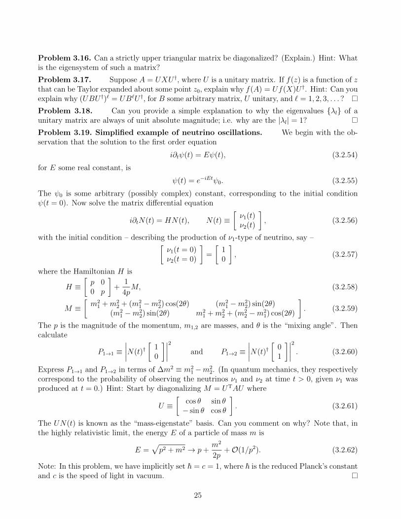
Problem 3.16. Can a strictly upper triangular matrix be diagonalized? (Explain.) Hint: Whatis the eigensystem of such a matrix?
Problem 3.17. Suppose A = UXU †, where U is a unitary matrix. If f(z) is a function of zthat can be Taylor expanded about some point z0, explain why f(A) = Uf(X)U †. Hint: Can youexplain why (UBU †)ℓ = UBℓU †, for B some arbitrary matrix, U unitary, and ℓ = 1, 2, 3, . . . ?
Problem 3.18. Can you provide a simple explanation to why the eigenvalues λl of aunitary matrix are always of unit absolute magnitude; i.e. why are the |λl| = 1?
Problem 3.19. Simplified example of neutrino oscillations. We begin with the ob-servation that the solution to the first order equation
i∂tψ(t) = Eψ(t), (3.2.54)
for E some real constant, is
ψ(t) = e−iEtψ0. (3.2.55)
The ψ0 is some arbitrary (possibly complex) constant, corresponding to the initial conditionψ(t = 0). Now solve the matrix differential equation
i∂tN(t) = HN(t), N(t) ≡[ν1(t)ν2(t)
], (3.2.56)
with the initial condition – describing the production of ν1-type of neutrino, say –[ν1(t = 0)ν2(t = 0)
]=
[10
], (3.2.57)
where the Hamiltonian H is
H ≡[p 00 p
]+
1
4pM, (3.2.58)
M ≡[m2
1 +m22 + (m2
1 −m22) cos(2θ) (m2
1 −m22) sin(2θ)
(m21 −m2
2) sin(2θ) m21 +m2
2 + (m22 −m2
1) cos(2θ)
]. (3.2.59)
The p is the magnitude of the momentum, m1,2 are masses, and θ is the “mixing angle”. Thencalculate
P1→1 ≡∣∣∣∣N(t)†
[10
]∣∣∣∣2 and P1→2 ≡∣∣∣∣N(t)†
[01
]∣∣∣∣2 . (3.2.60)
Express P1→1 and P1→2 in terms of ∆m2 ≡ m21 −m2
2. (In quantum mechanics, they respectivelycorrespond to the probability of observing the neutrinos ν1 and ν2 at time t > 0, given ν1 wasproduced at t = 0.) Hint: Start by diagonalizing M = UTAU where
U ≡[
cos θ sin θ− sin θ cos θ
]. (3.2.61)
The UN(t) is known as the “mass-eigenstate” basis. Can you comment on why? Note that, inthe highly relativistic limit, the energy E of a particle of mass m is
E =√p2 +m2 → p+
m2
2p+O(1/p2). (3.2.62)
Note: In this problem, we have implicitly set ℏ = c = 1, where ℏ is the reduced Planck’s constantand c is the speed of light in vacuum.
25
3.3 Special Topic: 2D real orthogonal matrices
In this subsection we will illustrate what a real orthogonal matrix is by studying the 2D casein some detail. Let A be such a 2 × 2 real orthogonal matrix. We will begin by writing itscomponents as follows
A ≡[v1 v2
w1 w2
]. (3.3.1)
(As we will see, it is useful to think of v1,2 and w1,2 as components of 2D vectors.) That A isorthogonal means AAT = I.[
v1 v2
w1 w2
]·[v1 w1
v2 w2
]=
[v · v v · ww · v w · w
]=
[1 00 1
]. (3.3.2)
This translates to: w2 ≡ w · w = 1, v2 ≡ v · v = 1 (length of both the 2D vectors are one);and w · v = 0 (the two vectors are perpendicular). In 2D any vector can be expressed in polarcoordinates; for example, the Cartesian components of v are
vi = r(cosϕ, sinϕ), r ≥ 0, ϕ ∈ [0, 2π). (3.3.3)
But v2 = 1 means r = 1. Similarly,
wi = (cosϕ′, sinϕ′), ϕ′ ∈ [0, 2π). (3.3.4)
Because v and w are perpendicular,
v · w = cosϕ · cosϕ′ + sinϕ · sinϕ′ = cos(ϕ− ϕ′) = 0. (3.3.5)
What we have figured out is that, any real orthogonal matrix can be parametrized by an angle0 ≤ ϕ < 2π; and for each ϕ there are two distinct solutions.
R1(ϕ) =
[cosϕ sinϕ− sinϕ cosϕ
], R2(ϕ) =
[cosϕ sinϕsinϕ − cosϕ
]. (3.3.7)
By a direct calculation you can check that R1(ϕ > 0) rotates an arbitrary 2D vector clockwiseby ϕ. Whereas, R2(ϕ > 0) rotates the vector, followed by flipping the sign of its y-component;this is because
R2(ϕ) =
[1 00 −1
]·R1(ϕ). (3.3.8)
In other words, the R2(ϕ = 0) in eq. (3.3.7) corresponds to a “parity flip” where the vector isreflected about the x-axis.
26
Problem 3.20. What about the matrix that reflects 2D vectors about the y-axis? Whatvalue of θ in R2(θ) would it correspond to?
Find the determinants of R1(ϕ) and R2(ϕ). You should be able to use that to argue, thereis no θ0 such that R1(θ0) = R2(θ0). Also verify that
R1(ϕ)R1(ϕ′) = R1(ϕ+ ϕ′). (3.3.9)
This makes geometric sense: rotating a vector clockwise by ϕ then by ϕ′ should be the same asrotation by ϕ+ϕ′. Mathematically speaking, this composition law in eq. (3.3.9) tells us rotationsform the SO2 group. The set of D × D real orthogonal matrices obeying RTR = I, includingboth rotations and reflections, forms the group OD. The group involving only rotations is knownas SOD; where the ‘S’ stands for “special” (≡ determinant equals one).
Problem 3.21. 2 × 2 Unitary Matrices. Can you construct the most general 2 × 2unitary matrix? First argue that the most general complex 2D vector v that satisfies v†v = 1 is
vi = eiϕ1(cos θ, eiϕ2 sin θ), ϕ1,2, θ ∈ [0, 2π). (3.3.10)
By taking the real and imaginary parts of this equation, argue that
ϕ′2 = ϕ2, θ = θ′ ± π
2. (3.3.13)
or
ϕ′2 = ϕ2 + π, θ = −θ′ ± π
2. (3.3.14)
From these, deduce that the most general 2 × 2 unitary matrix U can be built from the mostgeneral real orthogonal one O(θ) via
U =
[eiϕ1 00 eiϕ2
]·O(θ) ·
[1 00 eiϕ3
]. (3.3.15)
As a simple check: note that v†v = w†w = 1 together with v†w = 0 provides 4 constraintsfor 8 parameters – 4 complex entries of a 2 × 2 matrix – and therefore we should have 4 freeparameters left.
Bonus problem: By imposing detU = 1, can you connect eq. (3.3.15) to eq. (3.2.21)?
27
4 Linear Algebra
4.1 Definition
Loosely speaking, the notion of a vector space – as the name suggests – amounts to abstractingthe algebraic properties – addition of vectors, multiplication of a vector by a number, etc. –obeyed by the familiar D ∈ 1, 2, 3, . . . dimensional Euclidean space RD. We will discuss thelinear algebra of vector spaces using Paul Dirac’s bra-ket notation. This will not only help youunderstand the logical foundations of linear algebra and the matrix algebra you encounteredearlier, it will also prepare you for the study of quantum theory, which is built entirely on thetheory of both finite and infinite dimensional vector spaces.6
We will consider a vector space over complex numbers. A member of the vector space willbe denoted as |α⟩; we will use the words “ket”, “vector” and “state” interchangeably in whatfollows. We will allude to aspects of quantum theory, but point out everything we state hereholds in a more general context; i.e., quantum theory is not necessary but merely an application– albeit a very important one for physics. For now α is just some arbitrary label, but lateron it will often correspond to the eigenvalue of some linear operator. We may also use α asan enumeration label, where |α⟩ is the αth element in the collection of vectors. In quantummechanics, a physical system is postulated to be completely described by some |α⟩ in a vectorspace, whose time evolution is governed by some Hamiltonian. (The latter is what Schrodinger’sequation is about.)
Here is what defines a “vector space over complex numbers”. It is a collection of states|α⟩ , |β⟩ , |γ⟩ , . . . endowed with the operations of addition and scalar multiplication subject tothe following rules.
1. Ax1: Addition Any two vectors can be added to yield another vector
|α⟩+ |β⟩ = |γ⟩ . (4.1.1)
Addition is commutative and associative:
|α⟩+ |β⟩ = |β⟩+ |α⟩ (4.1.2)
|α⟩+ (|β⟩+ |γ⟩) = (|α⟩+ |β⟩) + |γ⟩ . (4.1.3)
2. Ax2: Additive identity (zero vector) and existence of inverse There is a zerovector |zero⟩ – which can be gotten by multiplying any vector by 0, i.e.,
0 |α⟩ = |zero⟩ (4.1.4)
– that acts as an additive identity.7 Namely, adding |zero⟩ to any vector returns the vectoritself:
|zero⟩+ |β⟩ = |β⟩ . (4.1.5)
6The material in this section of our notes was drawn heavily from the contents and problems provided inChapter 1 of Sakurai’s Modern Quantum Mechanics.
7In this section we will be careful and denote the zero vector as |zero⟩. For the rest of the notes, wheneverthe context is clear, we will often use 0 to denote the zero vector.
28
For any vector |α⟩ there exists an additive inverse; if + is the usual addition, then theinverse of |α⟩ is just (−1) |α⟩.
|α⟩+ (− |α⟩) = |zero⟩ . (4.1.6)
3. Ax3: Multiplication by scalar Any ket can be multiplied by an arbitrary complexnumber c to yield another vector
c |α⟩ = |γ⟩ . (4.1.7)
(In quantum theory, |α⟩ and c |α⟩ are postulated to describe the same system.) Thismultiplication is distributive with respect to both vector and scalar addition; if a and bare arbitrary complex numbers,
a(|α⟩+ |β⟩) = a |α⟩+ a |β⟩ (4.1.8)
(a+ b) |α⟩ = a |α⟩+ b |α⟩ . (4.1.9)
Note: If you define a “vector space over scalars,” where the scalars can be more general objectsthan complex numbers, then in addition to the above axioms, we have to add: (I) Associativity ofscalar multiplication, where a(b |α⟩) = (ab) |α⟩ for any scalars a, b and vector |α⟩; (II) Existenceof a scalar identity 1, where 1 |α⟩ = |α⟩.
Examples The Euclidean space RD itself, the space of D-tuples of real numbers
|a⟩ ≡ (a1, a2, . . . , aD), (4.1.10)
with + being the usual addition operation is, of course, the example of a vector space. We shallcheck explicitly that RD does in fact satisfy all the above axioms. To begin, let
|v⟩ = (v1, v2, . . . , vD),
|w⟩ = (w1, w2, . . . , wD) and (4.1.11)
|x⟩ = (x1, x2, . . . , xD) (4.1.12)
be vectors in RD.
1. Addition Any two vectors can be added to yield another vector
The following are some further examples of vector spaces.
1. The space of polynomials with complex coefficients.
2. The space of square integrable functions on RD (where D is an arbitrary integer greateror equal to 1); i.e., all functions f(x) such that
∫RD dDx|f(x)|2 <∞.
3. The space of all homogeneous solutions to a linear (ordinary or partial) differential equa-tion.
4. The space of M ×N matrices of complex numbers, where M and N are arbitrary integersgreater or equal to 1.
Problem 4.1. Prove that the examples in (1), (3), and (4) are indeed vector spaces, byrunning through the above axioms.
30
Linear (in)dependence, Basis, Dimension Suppose we pick N vectors from a vectorspace, and find that one of them (say, |N⟩) can be expressed as a linear combination (or,superposition) of the rest,
|N⟩ =N−1∑i=1
ci |i⟩ , (4.1.22)
where the χi are complex numbers. Then we say that this set of N vectors are linearlydependent. Equivalently, we may state that |1⟩ through |N⟩ are linearly dependent if a non-trivial superposition of them can be found to yield the zero vector:
N∑i=1
ci |i⟩ = |zero⟩ , ∃χi. (4.1.23)
That equations (4.1.22) and (4.1.23) are equivalent, is because – by assumption, cN = 0 – wecan divide eq. (4.1.23) throughout by cN ; similarly, we may multiply eq. (4.1.22) by cN .
Suppose we have picked D vectors |1⟩ , |2⟩ , |3⟩ , . . . , |D⟩ such that they are linearly inde-pendent, i.e., no vector is a linear combination of any others, and suppose further that anyarbitrary vector |α⟩ from the vector space can now be expressed as a linear combination (akasuperposition) of these vectors
|α⟩ =D∑i=1
ci |i⟩ , χi ∈ C. (4.1.24)
In other words, we now have a maximal number of linearly independent vectors – then, D iscalled the dimension of the vector space. The |i⟩ |i = 1, 2, . . . , D is a complete set of basisvectors; and such a set of (basis) vectors is said to span the vector space.8 It is worth reiterating,this is a maximal set because – if it were not, that would mean there is some additional vector|α⟩ that cannot be written as eq. (4.1.24).
Example For instance, for the D-tuple |a⟩ ≡ (a1, . . . , aD) from the real vector space ofRD, we may choose
The basis vectors are the |i⟩ and the dimension is D. Additionally, if we define
|v⟩ ≡ (1, 1, 0, . . . , 0) , (4.1.27)
|w⟩ ≡ (1,−1, 0, . . . , 0) , (4.1.28)
|u⟩ ≡ (1, 0, 0, . . . , 0) . (4.1.29)
8The span of vectors |1⟩ , . . . , |D⟩ is the space gotten by considering all possible linear combinations
∑D
i=1 ci |i⟩ |ci ∈ C.
31
We see that |v⟩ , |w⟩ are linearly independent – they are not proportional to each other – but|v⟩ , |w⟩ , |u⟩ are linearly dependent because
|u⟩ = 1
2|v⟩+ 1
2|w⟩ . (4.1.30)
Problem 4.2. Is the space of polynomials of complex coefficients of degree less than orequal to (n ≥ 1) a vector space? (Namely, this is the set of polynomials of the form Pn(x) =c0 + c1x + · · · + cnx
n, where the ci|i = 1, 2, . . . , n are complex numbers.) If so, write down aset of basis vectors. What is its dimension? Answer the same questions for the space of D ×Dmatrices of complex numbers.
Vector space within a vector space Before moving on to inner products, let us notethat a subset of a vector space is itself a vector space – i.e., a subspace of the larger vector space– if it is closed under addition and multiplication by complex numbers. Closure means, if |α⟩and |β⟩ are members of the subset, then c1 |α⟩+ c2 |β⟩ are also members of the same subset forany pair of complex numbers c1,2.
In principle, to understand why closure guarantees the subset is a subspace, we need to runthrough all the axioms in Ax1 through Ax3 above. But a brief glance tells us, the axioms in Ax1and Ax3 are automatically satisfied when closure is obeyed. Furthermore, closure means − |α⟩(i.e., the inverse of |α⟩) must lie within the subset whenever |α⟩ does, since the former is −1 times|α⟩. And that in turn teaches us, the zero vector gotten from superposing |α⟩+(−1) |α⟩ = |zero⟩must also lie within the subset. Namely, the set of axioms in Ax2 are, too, satisfied.
Examples The space of vectors |a⟩ = (a1, a2) in a 2D real space is a subspace of the3D counterpart |a⟩ = (a1, a2, a3); the former can be thought of as the latter with the thirdcomponent held fixed, a3 = same constant for all vectors. It is easy to check, the 2D vectors areclosed under linear combination.
We have already noted that the set of M × M matrices form a vector space. Therefore,the subset of Hermitian matrices over real numbers; or (anti)symmetric matrices over complex
numbers; must form subspaces. For, the superposition of Hermitian matrices H1, H2, . . . withreal coefficients yield another Hermitian matrix(
c1H1 + c2H2
)†= c1H1 + c2H2, c1,2 ∈ R; (4.1.31)
whereas the superposition of (anti)symmetric ones with complex coefficients return another(anti)symmetric matrix:(
c1H1 + c2H2
)T= c1H1 + c2H2, c1,2 ∈ C, HT
1,2 = H1,2, (4.1.32)(c1H1 + c2H2
)T= −(c1H1 + c2H2), c1,2 ∈ C, HT
1,2 = −H1,2. (4.1.33)
4.2 Inner Products
In Euclidean D-space RD the ordinary dot product, between the real vectors |a⟩ ≡ (a1, . . . , aD)
and |b⟩ ≡ (b1, . . . , bD), is defined as
a · b ≡D∑i=1
aibi = δijaibj. (4.2.1)
32
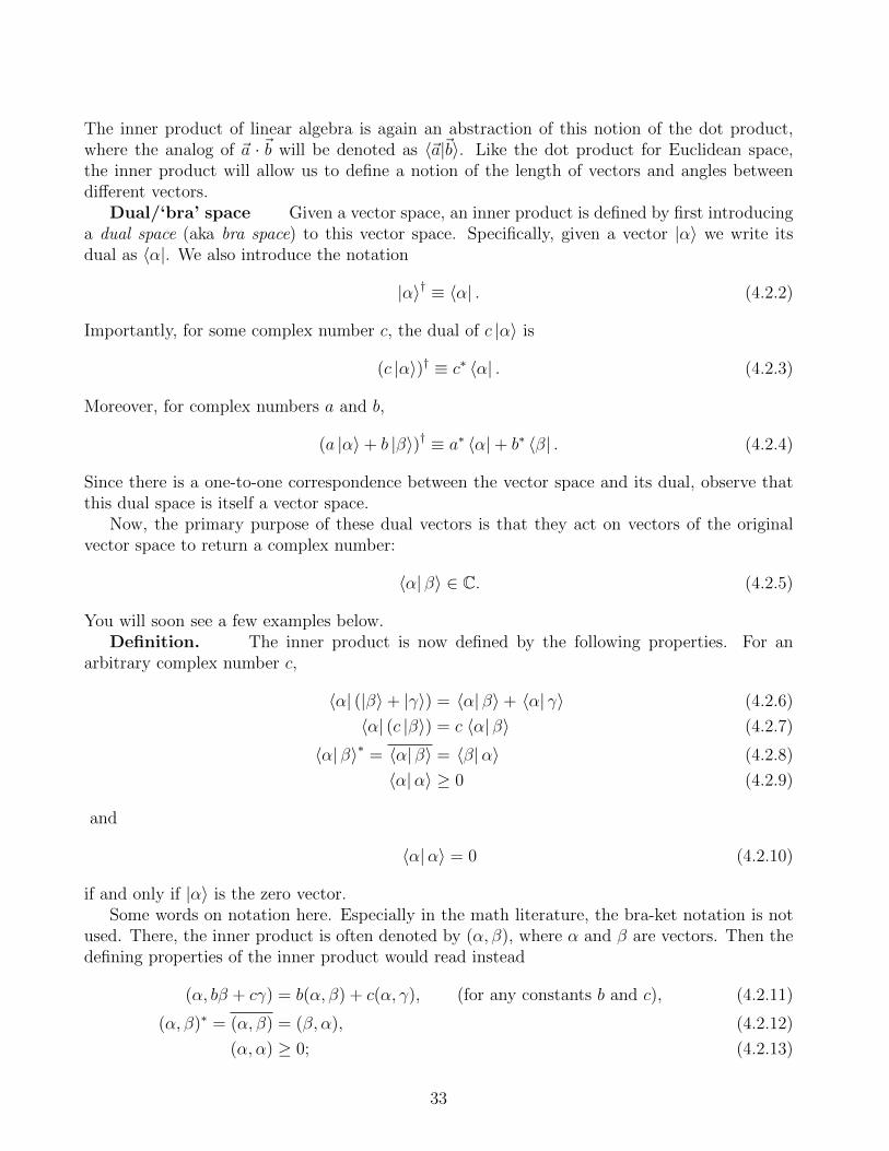
The inner product of linear algebra is again an abstraction of this notion of the dot product,where the analog of a · b will be denoted as ⟨a|b⟩. Like the dot product for Euclidean space,the inner product will allow us to define a notion of the length of vectors and angles betweendifferent vectors.
Dual/‘bra’ space Given a vector space, an inner product is defined by first introducinga dual space (aka bra space) to this vector space. Specifically, given a vector |α⟩ we write itsdual as ⟨α|. We also introduce the notation
|α⟩† ≡ ⟨α| . (4.2.2)
Importantly, for some complex number c, the dual of c |α⟩ is
(c |α⟩)† ≡ c∗ ⟨α| . (4.2.3)
Moreover, for complex numbers a and b,
(a |α⟩+ b |β⟩)† ≡ a∗ ⟨α|+ b∗ ⟨β| . (4.2.4)
Since there is a one-to-one correspondence between the vector space and its dual, observe thatthis dual space is itself a vector space.
Now, the primary purpose of these dual vectors is that they act on vectors of the originalvector space to return a complex number:
⟨α| β⟩ ∈ C. (4.2.5)
You will soon see a few examples below.Definition. The inner product is now defined by the following properties. For an
arbitrary complex number c,
⟨α| (|β⟩+ |γ⟩) = ⟨α| β⟩+ ⟨α| γ⟩ (4.2.6)
⟨α| (c |β⟩) = c ⟨α| β⟩ (4.2.7)
⟨α| β⟩∗ = ⟨α| β⟩ = ⟨β|α⟩ (4.2.8)
⟨α|α⟩ ≥ 0 (4.2.9)
and
⟨α|α⟩ = 0 (4.2.10)
if and only if |α⟩ is the zero vector.Some words on notation here. Especially in the math literature, the bra-ket notation is not
used. There, the inner product is often denoted by (α, β), where α and β are vectors. Then thedefining properties of the inner product would read instead
(α, bβ + cγ) = b(α, β) + c(α, γ), (for any constants b and c), (4.2.11)
(α, β)∗ = (α, β) = (β, α), (4.2.12)
(α, α) ≥ 0; (4.2.13)
33
and
(α, α) = 0 (4.2.14)
if and only if α is the zero vector. In addition, notice from equations (4.2.11) and (4.2.12) that
(bβ + cγ, α) = b∗(β, α) + c∗(γ, α). (4.2.15)
Example: Dot Product We may readily check that the ordinary dot product does, of course,satisfy all the axioms of the inner product. Firstly, let us denote
where all the components ai, bi, . . . are now real. Next, define
⟨a| b⟩= a · b = aTb. (4.2.19)
Then we may start with eq. (4.2.6): ⟨a| (|b⟩ + |c⟩) = ⟨a| b+ c⟩= a · b + a · c = ⟨a| b
⟩+ ⟨a| c⟩.
Second, ⟨a| (c∣∣∣b⟩) = ⟨a| cb
⟩= c(a · b) = c ⟨a| b
⟩. Third, ⟨a| b
⟩= a · b = b · a = (b · a)∗ =
⟨b∣∣∣ a⟩.
Fourth, ⟨a| a⟩ = a · a =∑
i(ai)2 is a sum of squares and therefore non-negative. Finally, because
⟨a| a⟩ is a sum of squares the only way it can be zero is for every component of a to be zero;moreover, if a is 0 then ⟨a| a⟩ = 0.
Problem 4.3. Prove that ⟨α|α⟩ is a real number. Hint: See eq. (4.2.8)
The following are examples of inner products.
Take the D-tuple of complex numbers |α⟩ ≡ (α1, . . . , αD) and∣∣∣β⟩ ≡ (β1, . . . , βD); and
define the inner product to be
⟨α| β⟩≡
D∑i=1
(αi)∗βi = δij(αi)∗βj = α†β. (4.2.20)
Consider the space of D×D complex matrices. Consider two such matrices X and Y anddefine their inner product to be ⟨
X∣∣∣ Y ⟩ ≡ Tr
[X†Y
]. (4.2.21)
Here, Tr means the matrix trace – i.e., summation over the diagonal components –
Tr [M ] ≡D∑i=1
M ii ≡M i
i; (4.2.22)
and X† is the matrix adjoint of X.
34
Consider the space of polynomials. Suppose |f⟩ and |g⟩ are two such polynomials of thevector space. Then
⟨f | g⟩ ≡∫ 1
−1
dxf(x)∗g(x) (4.2.23)
defines an inner product. Here, f(x) and g(x) indicates the polynomials are expressed interms of the variable x.
Problem 4.4. Prove the above examples are indeed inner products.
Problem 4.5. Prove the Cauchy-Schwarz inequality:
⟨α|α⟩ ⟨β| β⟩ ≥ |⟨α| β⟩|2 . (4.2.24)
The analogy in Euclidean space is |x|2|y|2 ≥ |x · y|2. Hint: Start with
(⟨α|+ c∗ ⟨β|) (|α⟩+ c |β⟩) ≥ 0. (4.2.25)
for any complex number c. (Why is this true?) Now choose an appropriate c to prove theSchwarz inequality.
Orthogonality Just as we would say two real vectors in RD are perpendicular (aka orthog-onal) when their dot product is zero, we may now define two vectors |α⟩ and |β⟩ in a vectorspace to be orthogonal when their inner product is zero:
⟨α| β⟩ = 0 = ⟨β|α⟩ . (4.2.26)
We also call the positive square root√
⟨α|α⟩ the norm of the vector |α⟩; recall, in Euclidean
space, the analogous |x| =√x · x. Given any vector |α⟩ that is not the zero vector, we can
always construct a vector from it that is of unit length,
|α⟩ ≡ |α⟩√⟨α|α⟩
⇒ ⟨α| α⟩ = 1. (4.2.27)
Suppose we are given a set of basis vectors |i′⟩ of a vector space. Through what is known asthe Gram-Schmidt process, one can always build from them a set of orthonormal basis vectors|i⟩; where every basis vector has unit norm and is orthogonal to every other basis vector,
⟨i| j⟩ = δij. (4.2.28)
As you will see, just as vector calculus problems are often easier to analyze when you choose anorthogonal coordinate system, linear algebra problems are often easier to study when you usean orthonormal basis to describe your vector space.
Problem 4.6. Suppose |α⟩ and |β⟩ are linearly dependent – they are scalar multiples ofeach other. However, their inner product is zero. What are |α⟩ and |β⟩?
35
Problem 4.7. Projection Process Let |1⟩ , |2⟩ , . . . , |N⟩ be a set of N orthonormalvectors. Let |α⟩ be an arbitrary vector lying in the same vector space. Show that the followingvector constructed from |α⟩ is orthogonal to all the |i⟩.
∣∣α⊥⟩ ≡ |α⟩ −N∑j=1
|j⟩ ⟨j|α⟩ (4.2.29)
This result is key to the following Gram-Schmidt process.
Gram-Schmidt Let |α1⟩ , |α2⟩ , . . . , |αD⟩ be a set of D linearly independent vectors thatspans some vector space. The Gram-Schmidt process is an iterative algorithm, based on theobservation in eq. (4.2.29), to generate from it a set of orthonormal set of basis vectors.
1. Take the first vector |α1⟩ and normalize it to unit length:
|α1⟩ =|α1⟩√⟨α1|α1⟩
. (4.2.30)
2. Take the second vector |α2⟩ and project out |α1⟩:∣∣α⊥2
⟩≡ |α2⟩ − |α1⟩ ⟨α1|α2⟩ , (4.2.31)
and normalize it to unit length
|α2⟩ ≡∣∣α⊥
2
⟩√⟨α⊥2
∣∣α⊥2
⟩ . (4.2.32)
3. Take the third vector |α3⟩ and project out |α1⟩ and |α2⟩:∣∣α⊥3
⟩≡ |α3⟩ − |α1⟩ ⟨α1|α3⟩ − |α2⟩ ⟨α2|α3⟩ , (4.2.33)
then normalize it to unit length
|α3⟩ ≡∣∣α⊥
3
⟩√⟨α⊥3
∣∣α⊥3
⟩ . (4.2.34)
4. Repeat . . . Take the ith vector |αi⟩ and project out |α1⟩ through |αi−1⟩:
∣∣α⊥i
⟩≡ |αi⟩ −
i−1∑j=1
|αj⟩ ⟨αj|αi⟩ , (4.2.35)
then normalize it to unit length
|αi⟩ ≡∣∣α⊥
i
⟩√⟨α⊥i
∣∣α⊥i
⟩ . (4.2.36)
36
By construction, |αi⟩ will be orthogonal to |α1⟩ through |αi−1⟩. Therefore, at the end of theprocess, we will have D mutually orthogonal and unit norm vectors. Because they are orthogonalthey are linearly independent – hence, we have succeeded in constructing an orthonormal set ofbasis vectors.
Example Here is a simple example in 3D Euclidean space endowed with the usual dotproduct. Let us have
You can check that these vectors are linearly independent by taking the determinant of the 3×3matrix formed from them. Alternatively, the fact that they generate a set of basis vectors fromthe Gram-Schmidt process also implies they are linearly independent.
Problem 4.8. Consider the space of polynomials with complex coefficients. Let the innerproduct be
⟨f | g⟩ ≡∫ +1
−1
dxf(x)∗g(x). (4.2.44)
Starting from the set |0⟩ = 1, |1⟩ = x, |2⟩ = x2, construct from them a set of orthonormalbasis vectors spanning the subspace of polynomials of degree equal to or less than 2. Compareyour results with the Legendre polynomials
Pℓ(x) ≡1
2ℓℓ!
dℓ
dxℓ(x2 − 1
)ℓ, ℓ = 0, 1, 2. (4.2.45)
Orthogonality and Linear independence. We close this subsection with an ob-servation. If a set of non-zero kets |i⟩ |i = 1, 2, . . . , N − 1, N are orthogonal, then they arenecessarily linearly independent. This can be proved readily by contradiction. Suppose thesekets were linearly dependent. Then it must be possible to find non-zero complex numbers Cisuch that
N∑i=1
Ci |i⟩ = 0. (4.2.46)
If we now act ⟨j| on this equation, for any j ∈ 1, 2, 3, . . . , N,N∑i=1
Ci ⟨j| i⟩ =N∑i=1
Ciδij ⟨j| j⟩ = Cj ⟨j| j⟩ = 0. (4.2.47)
That means all the Cj|j = 1, 2, . . . , N are in fact zero.A simple application of this observation is, if you have found D mutually orthogonal kets
|i⟩ in a D dimensional vector space, then these kets form a basis. By normalizing them tounit length, you’d have obtained an orthonormal basis. Such an example is that of the Paulimatrices σµ|µ = 0, 1, 2, 3 in eq. (3.2.15). The vector space of 2 × 2 complex matrices is 4-dimensional, since there are 4 independent components. Moreover, we have already seen thatthe trace Tr
[X†Y
]is one way to define an inner product of matrices X and Y . Since
1
2Tr[(σµ)† σν
]=
1
2Tr [σµσν ] = δµν , µ, ν ∈ 0, 1, 2, 3, (4.2.48)
that means, by the argument just given, the 4 Pauli matrices σµ form an orthogonal set ofbasis vectors for the vector space of complex 2× 2 matrices. That means it must be possible tochoose pµ such that the superposition pµσ
µ is equal to any given 2× 2 complex matrix A. Infact,
pµσµ = A ⇔ pµ =
1
2Tr [σµA] . (4.2.49)
In quantum mechanics and quantum field theory, these σµ are fundamental to describingspinors and spin−1/2 systems.
38
4.3 Linear Operators
4.3.1 Definitions and Fundamental Concepts
In quantum theory, a physical observable is associated with a (Hermitian) linear operator actingon the vector space. What defines a linear operator? If A is one, it is primarily defined by howit acts from the left on a vector to return another vector
A |α⟩ = |α′⟩ . (4.3.1)
In other words, if you can tell me what the ‘output’ |α′⟩ is, after A acts on any vector of thevector space |α⟩ – you’d have defined A itself. But that’s not all – linearity also means, forotherwise arbitrary operators A and B and complex numbers c and d,
(c A+ d B) |α⟩ = c A |α⟩+ d B |α⟩ (4.3.2)
A(c |α⟩+ d |β⟩) = c A |α⟩+ d A |β⟩ .
If X and Y are both linear operators, since Y |α⟩ is a vector, we can apply X to it to obtainanother vector, X(Y |α⟩). This means we ought to be able to multiply operators, for e.g., XY .We will assume this multiplication is associative, namely
XY Z = (XY )Z = X(Y Z). (4.3.3)
Identity The identity operator obeys
I |γ⟩ = |γ⟩ for all |γ⟩. (4.3.4)
Inverse The inverse of the operator X is still defined as one that obeys
X−1X = XX−1 = I. (4.3.5)
Strictly speaking, we need to distinguish between the left and right inverse, but in finite dimen-sional vector spaces, they are the same object.Adjoint Next, let us observe that an operator always acts on a bra from the right, andreturns another bra,
⟨α|A = ⟨α′| . (4.3.6)
The reason is that a bra is something that acts linearly on an arbitrary vector and returns acomplex number. Since that is what ⟨α|A does, it must therefore some bra ‘state’.
To formalize this further, we shall denote the adjoint of the linear operator X, namely X†,by taking the † of the ket X† |α⟩ in the following way:
(X† |α⟩)† = ⟨α|X. (4.3.7)
If |α⟩ and |β⟩ are arbitrary states,
⟨β |X|α⟩ = ⟨β| (X |α⟩) =(X† |β⟩
)† |α⟩ . (4.3.8)
39
In words: Given a linear operator X, its adjoint X† is defined as the operator that – after actingupon |β⟩ – would yield an inner product (X† |β⟩)† |α⟩ which is equal to ⟨β| (X |α⟩). As we shallsee below, an equivalent manner to define the adjoint is either
⟨α|X |β⟩ = ⟨β|X† |α⟩ (4.3.9)
or ⟨α|X† |β⟩ = ⟨β|X |α⟩ . (4.3.10)
Why such a definition yields a unique operator X† would require some explanation; in a similarvein, we shall see below that,
(X†)† = X. (4.3.11)
Hence, we could also have began with the definition
(X |α⟩)† = ⟨α|X†. (4.3.12)
In the math literature, where α and β denote the states and X is still some linear operator, thelatter’s adjoint is expressed through the inner product as
(β,Xα) =(X†β, α
). (4.3.13)
Problem 4.9. Prove that
(XY )† = Y †X†. (4.3.14)
Hint: take the adjoint of (XY )† |α⟩ and Y †(X† |α⟩).
Eigenvectors and eigenvalues An eigenvector of some linear operator A is a vector that,when acted upon by A, returns the vector itself multiplied by a complex number a:
X |a⟩ = a |a⟩ . (4.3.15)
This number a is called the eigenvalue of A.Remark The eigenvector is not unique, in that we may always multiply it by an arbitrary
complex number z and still obtain an eigenvector:
X (z |a⟩) = a(z |a⟩). (4.3.16)
In quantum mechanics we require the state to be normalized to unity, i.e., ⟨a| a⟩ = 1 =⟨a| z∗z |a⟩ = |z|2 ⟨a| a⟩. This |z| = ±1 constraint implies that unit norm eigenvectors maydiffer by a phase.
X(eiθ |a⟩
)= a(eiθ |a⟩), θ ∈ R. (4.3.17)
Ket-bra operator Notice that the product |α⟩ ⟨β| can be considered a linear operator. Tosee this, we apply it on some arbitrary vector |γ⟩ and observe it returns the vector |α⟩ multipliedby a complex number describing the projection of |γ⟩ on |β⟩,
as long as we assume these products are associative. It obeys the following “linearity” rules. If|α⟩ ⟨β| and |α′⟩ ⟨β′| are two different ket-bra operators,
|α⟩ ⟨β| (c |γ⟩+ d |γ′⟩) = c |α⟩ ⟨β| γ⟩+ d |α⟩ ⟨β| γ′⟩ . (4.3.20)
Problem 4.10. Show that
(|α⟩ ⟨β|)† = |β⟩ ⟨α| . (4.3.21)
Hint: Act (|α⟩ ⟨β|)† on an arbitrary vector, and then take its adjoint.
Projection operator The special case |α⟩ ⟨α| acting on any vector |γ⟩ will return|α⟩ ⟨α| γ⟩. Thus, we can view it as a projection operator – it takes an arbitrary vector andextracts the portion of it “parallel” to |α⟩.
Superposition, the Identity operator as a completeness relation We will nowsee that (square) matrices can be viewed as representations of linear operators on a vector space.Let |i⟩ denote the basis orthonormal vectors of the vector space,
⟨i| j⟩ = δij. (4.3.22)
Then we may consider acting an linear operator X on some arbitrary vector |γ⟩, which we willexpress as a linear combination of the |i⟩:
|γ⟩ =∑i
γi |i⟩ , γi ∈ C. (4.3.23)
By acting both sides with respect to ⟨j|, we have
⟨j| γ⟩ = γj. (4.3.24)
In other words,
|γ⟩ =∑i
|i⟩ ⟨i| γ⟩ =
(∑i
|i⟩ ⟨i|
)|γ⟩ . (4.3.25)
Since |γ⟩ was arbitrary, we have identified the identity operator as
I =∑i
|i⟩ ⟨i| . (4.3.26)
This is also often known as a completeness relation: summing over the ket-bra projection oper-ators built out of the orthonormal basis vectors of a vector space returns the unit (aka identity)operator. I acting on any vector yields the same vector.
Representations, Vector components, Matrix elements Once a set of orthonormalbasis vectors are chosen, notice from the expansion in eq. (4.3.25), that to specify a vector |γ⟩
41
all we need to do is to specify the complex numbers ⟨i| γ⟩. These can be arranged as a columnvector; if the dimension of the vector space is D, then
|γ⟩ =
⟨1| γ⟩⟨2| γ⟩⟨3| γ⟩. . .
⟨D| γ⟩
. (4.3.27)
The = is not quite an equality; rather it means “represented by,” in that this column vectorcontains as much information as eq. (4.3.25), provided the orthonormal basis vectors are known.
We may also express an arbitrary bra through a superposition of the basis bras ⟨i|, usingthe adjoint of eq. (4.3.26).
⟨α| =∑i
⟨α| i⟩ ⟨i| . (4.3.28)
(According to eq. (4.3.26), this is simply ⟨α| I.) In this case, the coefficients ⟨α| i⟩ may bearranged as a row vector:
⟨α| =[⟨α| 1⟩ ⟨α| 2⟩ . . . ⟨α|D⟩
]. (4.3.29)
Inner products Let us consider the inner product ⟨α| γ⟩. By inserting the completenessrelation in eq. (4.3.26), we obtain
⟨α| γ⟩ =∑i
⟨α| i⟩ ⟨i| γ⟩ = δij(αi)∗γj = α†γ, (4.3.30)
αi ≡ ⟨i|α⟩ , γj ≡ ⟨j| γ⟩ . (4.3.31)
This is the reason for writing a ket |γ⟩ as a column whose components are its representation (eq.(4.3.27)) and a bra ⟨α| as a row whose components are the complex conjugate of its representation(eq. (4.3.29)) – their inner product is in fact the complex ‘dot product’
⟨α| γ⟩ =
⟨1|α⟩⟨2|α⟩. . .
⟨D|α⟩
†
⟨1| γ⟩⟨2| γ⟩. . .
⟨D| γ⟩
, (4.3.32)
where the dagger here refers to the matrix algebra operation of taking the transpose and complexconjugation, for e.g. v† = (vT)∗. Furthermore, if |γ⟩ has unit norm, then
1 = ⟨γ| γ⟩ =∑i
⟨γ| i⟩ ⟨i| γ⟩ =∑i
|⟨i| γ⟩|2 =δij(γi)∗γj = γ†γ. (4.3.33)
Linear operators Next, consider some operatorX acting on an arbitrary vector |γ⟩, expressedthrough the orthonormal basis vectors |i⟩. We can insert identity operators, one from the leftand another from the right of X,
X |γ⟩ =∑i,j
|j⟩ ⟨j |X| i⟩ ⟨i| γ⟩ . (4.3.34)
42
We can also apply the lth basis bra ⟨l| from the left on both sides and obtain
⟨l|X |γ⟩ =∑i
⟨l |X| i⟩ ⟨i| γ⟩ . (4.3.35)
Just as we read off the components of the vector in eq. (4.3.25) as a column vector, we can dothe same here. Again supposing a D dimensional vector space for notational convenience,
In words: X acting on some vector |γ⟩ can be represented by the column vector gotten fromacting the matrix ⟨j |X| i⟩, with row number j and column number i, acting on the columnvector ⟨i| γ⟩. In index notation, with9
X ij ≡ ⟨i |X| j⟩ and γj ≡ ⟨j| γ⟩ , (4.3.37)
we have
⟨i|X |γ⟩ =X ij γ
j. (4.3.38)
Since |γ⟩ in eq. (4.3.34) was arbitrary, we may record that any linear operator X admits anket-bra operator expansion:
X =∑i,j
|j⟩ ⟨j |X| i⟩ ⟨i| =∑i,j
|j⟩ Xji ⟨i| . (4.3.39)
We have already seen, this result follows from inserting the completeness relation in eq. (4.3.26)
on the left and right ofX. Importantly, notice that specifying the matrix Xji amounts to defining
the linear operator X itself, once a orthonormal basis has been picked.As an example: what is the matrix representation of |β⟩ ⟨α|? We apply ⟨i| from the left and
Products of Linear Operators We can consider Y X, where X and Y are linear operators.By inserting the completeness relation in eq. (4.3.26),
Y X |γ⟩ =∑i,j,k
|k⟩ ⟨k|Y |j⟩ ⟨j |X| i⟩ ⟨i| γ⟩
=∑k
|k⟩ Y kjX
jiγ
i. (4.3.41)
9In this chapter on the abstract formulation of Linear Algebra, I use a · to denote a matrix (representation),in order to distinguish it from the linear operator itself.
Notice how the rules of matrix multiplication emerges from this abstract formulation of linearoperators acting on a vector space.
Adjoint Finally, we may now understand how to construct the matrix representation ofthe adjoint of a given linear operator X by starting from eq. (4.3.8) with orthonormal states|i⟩. Firstly, from eq. (4.3.39),
X† |i⟩ =∑a,b
|a⟩ (X†)ab ⟨b| i⟩ =∑a
|a⟩ (X†)ai. (4.3.43)
Taking the † using eq. (4.2.3), and then applying it to |j⟩,
(X† |i⟩)† |j⟩ =∑a
(X†)ai ⟨a| j⟩ = (X†)ji. (4.3.44)
According to eq. (4.3.8), this must be equal to ⟨i |X| j⟩ = X ij. This, of course, coincides with
the definition of the adjoint from matrix algebra: the representation of the adjoint of X is thecomplex conjugate and transpose of that of X:⟨
j∣∣X†∣∣ i⟩ = ⟨i |X| j⟩∗ ⇔ X† =
(XT)∗. (4.3.45)
Because the matrix representation of a linear operator within an orthonormal basis is unique,notice we have also provided a constructive proof of the uniqueness of X† itself. We could alsohave obtained eq. (4.3.45) more directly by starting with the ket-bra expansion (cf. (4.3.39)) ofX and then using equations (4.2.3) and (4.3.21) to directly implement † on the right hand side:
X† =∑i,j
((X i
j |i⟩) ⟨j|)†
(4.3.46)
=∑i,j
|j⟩ X ij ⟨i| ≡
∑i,j
|j⟩ (X†)ji ⟨i| . (4.3.47)
Problem 4.11. Adjoint of an adjoint Prove that (X†)† = X.
Now that you have shown that (Y †)† = Y for any linear operator Y , for any states |α⟩ and|β⟩; and for any linear operator X, we may recover eq. (4.3.9) from the property ⟨α| γ⟩ = ⟨γ|α⟩:
Vector Space of Linear Operators You may step through the axioms of Linear Algebrato verify that the space of Linear operators is, in fact, a vector space itself. (More specifically,
44
we have just seen that linear operators may be represented by D×D square matrices, which inturn span a vector space of dimension D2.) Given an orthonormal basis |i⟩ for the originalvector space upon which these linear operators are acting, the expansion in eq. (4.3.39) – whichholds for an arbitrary linear operator X – teaches us the set of D2 ket-bra operators
|j⟩ ⟨i| |j, i = 1, 2, 3, . . . , D (4.3.49)
form the basis of the space of linear operators. The matrix elements ⟨j |X| i⟩ = Xji are the
expansion coefficients.
The set of linear operators X acting on a D−dimensional vector space is itselfa D2 dimensional vector space, because they are represented by the set of D × Dmatrices X i
j = ⟨i |X| j⟩.
Inner Product of Linear Operators We have already witnessed how the trace operation
may be used to define an inner product between matrices:⟨A∣∣∣ B⟩ = Tr
[A†B
]. Let us now
define the trace of a linear operator X to be
Tr [X] ≡D∑ℓ=1
⟨ℓ |X| ℓ⟩ ; (4.3.50)
where the |ℓ⟩ form an orthonormal basis. (That any orthonormal basis would do – i.e., this isa basis independent definition, as along as the basis is unit norm and mutually perpendicular –will be proven in the section on unitary operators below.) We may now define the inner productbetween two linear operators X and Y as
⟨X|Y ⟩ ≡ Tr[X†Y
]. (4.3.51)
This is in fact equivalent to the matrix trace inner product because, by inserting the completenessrelation (4.3.26) between X and Y and employing eq. (4.3.50),
⟨X|Y ⟩ =∑i,j
⟨i|X† |j⟩ ⟨j|Y |i⟩ = (X†)ijYji = Tr
[X†Y
]. (4.3.52)
With such a tool, it is now possible to sharpen the statement that the set of D2 ket-bra operators|i⟩ ⟨j| |i, j ∈ 1, 2, 3, . . . , D form an orthonormal basis for the vector space of linear operators.Recall: since the dimension of such a space is D2, all we have to show is the linear independenceof this set. But this in turn follows if they are orthonormal. Hence, consider the inner productbetween |i⟩ ⟨j| and |m⟩ ⟨n|. Utilizing the result that (|i⟩ ⟨j|)† = |j⟩ ⟨i|:
Tr[(|i⟩ ⟨j|)†(|m⟩ ⟨n|)
]=∑ℓ
⟨ℓ| j⟩ ⟨i|m⟩ ⟨n| ℓ⟩ . (4.3.53)
Now, by assumption, ⟨ℓ| j⟩ is non-zero only when ℓ = j. Similarly, ⟨n| ℓ⟩ is non-zero only whenℓ = n. Therefore when j = n the entire sum is zero because ℓ cannot be simultaneously equalto both j and n. But again by the orthonormal assumption, when ℓ = j = n, ⟨ℓ| j⟩ ⟨n| ℓ⟩ = 1.
45
In other words, the sum is proportional to δjn; likewise ⟨i|m⟩ = δim too. At this point, we havearrived at the orthonormality condition:
Tr[(|i⟩ ⟨j|)†(|m⟩ ⟨n|)
]= δimδ
jn. (4.3.54)
The kets must be identical and so must the bras; otherwise these ket-bra linear operators areperpendicular.
Problem 4.12. Throughout this section, we are focusing on linear operators that act on a ketand return another within the same vector space; hence, their matrix representations are D×Dmatrices. Suppose a linear operator acts on kets within a N dimensional vector space but returnsa ket from a (different) M dimensional one. What is the size of the matrix representation?
Mapping finite dimensional vector spaces to CD Let us pause to summarize ourpreceding discussion. Even though it is possible to discuss finite dimensional vector spacesin the abstract, it is always possible to translate the setup at hand to one of the D-tuple ofcomplex numbers, where D is the dimensionality. First choose a set of orthonormal basis vectors|1⟩ , . . . , |D⟩. Then, every vector |α⟩ can be represented as a column vector; the ith componentis the result of projecting the abstract vector on the ith basis vector ⟨i|α⟩; conversely, writing acolumn of complex numbers can be interpreted to define a vector in this orthonormal basis. Theinner product between two vectors ⟨α| β⟩ =
∑i ⟨α| i⟩ ⟨i| β⟩ boils down to the complex conjugate
of the ⟨i|α⟩ column vector dotted into the ⟨i| β⟩ vector. Moreover, every linear operator O canbe represented as a matrix with the element on the ith row and jth column given by ⟨i |O| j⟩;and conversely, writing any square matrix Oi
j can be interpreted to define a linear operator, onthis vector space, with matrix elements ⟨i |O| j⟩. Product of linear operators becomes productsof matrices, with the usual rules of matrix multiplication.
Differentiating kets, bras, and linear operators Suppose a ket |ψ(t)⟩ depends on acontinuous real parameter t. Then it should make sense to define the limit
∂t |ψ(t)⟩ ≡ limδt→0
|ψ(t+ δt)⟩ − |ψ(t)⟩δt
. (4.3.55)
Taking the adjoint on both sides hands us the corresponding definition for the derivative of thebra.
∂t ⟨ψ(t)| ≡ limδt→0
⟨ψ(t+ δt)| − ⟨ψ(t)|δt
= (∂t |ψ(t)⟩)† . (4.3.56)
46
Likewise, the derivative of a linear operator A(t) that depends on a real continuous parametert may be defined as
∂tA(t) = limδt→0
A(t+ δt)− A(t)
δt. (4.3.57)
Problem 4.13. Product rule Can you prove the product rule holds for the derivative ofmatrix elements; i.e.,
Explain why the derivative of the adjoint of a linear operator is the adjoint of the derivative ofthe same operator: (∂tA(t))
† = ∂tA†.
Next we highlight two special types of linear operators that play central roles in quantum theory:hermitian and unitary operators.
4.3.2 Hermitian Operators
A hermitian linear operator X is one that is equal to its own adjoint, namely
X† = X. (4.3.59)
From eq. (4.3.9), we see that a linear operator X is hermitian if and only if
⟨α|X |β⟩ = ⟨β|X |α⟩∗ (4.3.60)
for arbitrary vectors |α⟩ and |β⟩. In particular, if |i⟩ |i = 1, 2, 3, . . . , D form an orthonormalbasis, we recover the definition of a Hermitian matrix,
⟨j|X |i⟩ = ⟨i|X |j⟩∗ . (4.3.61)
We now turn to the following important facts about Hermitian operators.
Hermitian Operators Have Real Spectra: If X is a Hermitian operator,all its eigenvalues are real and eigenvectors corresponding to different eigenvalues areorthogonal.
Proof Let |a⟩ and |a′⟩ be eigenvectors of X, i.e.,
X |a⟩ = a |a⟩ (4.3.62)
Taking the adjoint of the analogous equation for |a′⟩, and using X = X†,
⟨a′|X = a′∗ ⟨a′| . (4.3.63)
We can multiply ⟨a′| from the left on both sides of eq. (4.3.62); and multiply |a⟩ from the righton both sides of eq. (4.3.63).
Suppose the eigenvalues are the same, a = a′. Then 0 = (a − a∗) ⟨a| a⟩; because |a⟩ is not anull vector, this means a = a∗; eigenvalues of Hermitian operators are real. Suppose insteadthe eigenvalues are distinct, a = a′. Because we have just proven that a′ can be assumed tobe real, we have 0 = (a − a′) ⟨a′| a⟩. By assumption the factor a − a′ is not zero. Therefore⟨a′| a⟩ = 0, namely, eigenvectors corresponding to different eigenvalues of a Hermitian operatorare orthogonal.
Completeness of Hermitian Eigensystem:10 The eigenkets |λk⟩ |k =1, 2, . . . , D of a Hermitian operator span the vector space upon which it is acting.The full set of eigenvalues λk|k = 1, 2, . . . , D of some Hermitian operator is calledits spectrum; and from eq. (4.3.26), completeness of its eigenvectors reads
I =D∑
k=1
|λk⟩ ⟨λk| . (4.3.66)
In the language of matrix algebra, we’d say that a Hermitian matrix is always diag-onalizable via a unitary transformation.
In quantum theory, we postulate that (many) observables such as spin, position, momentum,etc., correspond to Hermitian operators; their eigenvalues are then the possible outcomes of themeasurements of these observables. (It is not possible to obtain a measurement correspondingto X that is not its eigenvalue.) Since their spectrum are real, this guarantees we get a realnumber from performing a measurement on the system at hand. That the eigenstates of anobservable span the given vector space also means the range of physical states correspondingto possible measurement outcomes may be employed to fully characterize the dynamics of thequantum system itself.
Degeneracy and Symmetry If more than one eigenket of A has the same eigenvalue,we say A’s spectrum is degenerate. The simplest example is the identity operator itself: everybasis vector is an eigenvector with eigenvalue 1. The matrix diag[1, π, 2, 2] is degenerate: it actson a 4D vector space with two repeated eigenvalues.
When an operator is degenerate, the labeling of eigenkets using their eigenvalues becomeambiguous – which eigenket does |λ⟩ correspond to, if this subspace is 5 dimensional, say?What often happens is that one can find a different observable B to distinguish between theeigenkets of the same λ. For example, we will see below that the negative Laplacian on the 2-sphere – known as the “square of total angular momentum,” when applied to quantum mechanics– will have eigenvalues ℓ(ℓ+1), where ℓ ∈ 0, 1, 2, 3, . . . . It will also turn out to be (2ℓ+1)-folddegenerate, but this degeneracy can be labeled by an integer m, corresponding to the eigenvaluesof the generator-of-rotation about the North pole J(ϕ) (where ϕ is the azimuthal angle). A closely
related fact is that [−∇2S2 , J(ϕ)] = 0, where [X, Y ] ≡ XY − Y X.
− ∇2S2 |ℓ,m⟩ = ℓ(ℓ+ 1) |ℓ,m⟩ , (4.3.67)
10The most general type of operator that is diagonalizable is a normal operator, defined as one that commuteswith its own adjoint. Both Hermitian and Unitary (discussed in §(4.3.3) below) operators are normal. I provethe diagonalizability of normal operators in §(4.10).
It’s worthwhile to mention, in the context of quantum theory – degeneracy in the spectrum isoften associated with the presence of symmetry. For example, the Stark and Zeeman effectscan be respectively thought of as the breaking of rotational symmetry of an atomic system by,respectively, a non-zero magnetic and electric field. Previously degenerate spectral lines becomesplit into distinct ones, due to these E and B fields.11 In the context of classical field theory, wewill witness in the section on continuous vector spaces below, how the translation invariance ofspace leads to a degenerate spectrum of the Laplacian.
Problem 4.14. Let X be a linear operator with eigenvalues λi|i = 1, 2, 3, . . . , D andorthonormal eigenvectors |λi⟩ |i = 1, 2, 3, . . . , D that span the given vector space. Show thatX can be expressed as
X =∑i
λi |λi⟩ ⟨λi| . (4.3.68)
(Assume a non-degenerate spectra for now.) Verify that the right hand side is represented by adiagonal matrix in this basis |λi⟩. Of course, a Hermitian linear operator is a special case of eq.(4.3.68), where all the λi are real. Hint: Given that the eigenkets of X span the vector space,all you need to verify is that all possible matrix elements of X return what you expect.
How to diagonalize a Hermitian operator? To diagonalize a linear operator X meansto get it in the form in eq. (4.3.68), where it is expanded in terms of projectors built out of itseigen-kets |λi⟩. The matrix representation in such a basis is purely diagonal ⟨λi |X|λj⟩ = λiδ
ij.
Suppose you are given a Hermitian operator H in some orthonormal basis |i⟩, namely
H =∑i,j
|i⟩ H ij ⟨j| =
∑i,j
|i⟩ ⟨i |H| j⟩ ⟨j| . (4.3.69)
How does one go about diagonalizing it? Here is where the matrix algebra you are familiar withcomes in – recall the discussion leading up to eq. (3.2.37). By treating H i
j as a matrix, you canfind its eigenvectors and eigenvalues λk. Specifically, what you are solving for is the unitary
matrix U jk, whose kth column is the kth unit length eigenvector of H i
j, with eigenvalue λk:
H ijU
jk = λkU
jk ⇔
∑j
⟨i |H| j⟩ ⟨j|λk⟩ = λk ⟨i|λk⟩ , (4.3.70)
with
⟨i |H| j⟩ ≡ H ij and ⟨j|λk⟩ ≡ U j
k. (4.3.71)
In other words,
H ij = (Udiag[λ1, . . . , λD]U
†)ij
11See Wikipedia articles on the Stark and Zeeman effects for plots of the energy levels vs. electric/magneticfield strengths.
Once you have obtained the representation of the kth eigenket U ik = (⟨1|λk⟩ , ⟨2|λk⟩ , . . . , ⟨D|λk⟩)T,
you can then write the eigenket itself as
|λk⟩ =∑i
|i⟩ ⟨i|λk⟩ =∑i
|i⟩ U ik. (4.3.73)
The adjoint of the same eigenket is
⟨λk| =∑i
⟨λk| i⟩ ⟨i| =∑i
U ik ⟨i| =
∑i
(U †)ki ⟨i| . (4.3.74)
The operator H has now been diagonalized as
H =∑k
λk |λk⟩ ⟨λk| (4.3.75)
because according to eq. (4.3.72),
H =∑i,j
|i⟩ H ij ⟨j| =
∑i,j,a
|i⟩ ⟨i|λa⟩λa ⟨λa| j⟩ ⟨j| . (4.3.76)
Using the completeness relation in eq. (4.3.26) then leads us to eq. (4.3.75).In summary, with the relations in eq. (4.3.71),
H =∑i,j
|i⟩ H ij ⟨j| =
∑k
λk |λk⟩ ⟨λk| (4.3.77)
=∑
i,j,m,n
|i⟩ U im (diag [λ1, . . . , λD])
mn (U
†)nj ⟨j| . (4.3.78)
This matrix algebra that guarantees every Hermitian matrix can be diagonalized through aunitary transformation, H = Udiag[λ1, . . . , λD]U
†, also amounts to a proof that all Hermitianoperators acting on finite dimensional vector spaces have a complete spectra – since, the columnsof U are the (representation of) the orthonormal eigenbasis.
Problem 4.15. Consider a 2 dimension vector space with the orthonormal basis |1⟩ , |2⟩. Theoperator H is defined through its actions:
H |1⟩ = a |1⟩+ ib |2⟩ , (4.3.79)
H |2⟩ = −ib |1⟩+ a |2⟩ ; (4.3.80)
where a and b are real numbers. Is H hermitian? What are its eigenvectors and eigenvalues?
Compatible observables Let X and Y be observables – aka Hermitian operators. Weshall define compatible observables to be ones where the operators commute,
[A,B] ≡ AB −BA = 0. (4.3.81)
They are incompatible when [A,B] = 0. Finding the maximal set of mutually compatible set ofobservables in a given physical system will tell us the range of eigenvalues that fully capture thequantum state of the system. To understand this we need the following result.
50
Theorem Suppose X and Y are observables – they are Hermitian operators.Then X and Y are compatible (i.e., commute with each other) if and only if theyare simultaneously diagonalizable.
Proof We will provide the proof for the case where the spectrum of X is non-degenerate.We have already stated earlier that if X is Hermitian we can expand it in its basis eigenkets.
X =∑a
a |a⟩ ⟨a| (4.3.82)
In this basis X is already diagonal. But what about Y ? Suppose [X, Y ] = 0. We consider, fordistinct eigenvalues a and a′ of X,
⟨a′ |[X, Y ]| a⟩ = ⟨a′ |XY − Y X| a⟩ = (a′ − a) ⟨a′ |Y | a⟩ = 0. (4.3.83)
Remember, all eigenvalues of X and Y are real because the operators are Hermitian; hence notonly X |a⟩ = a |a⟩ we also have ⟨a′|X = (X† |a′⟩)† = (X |a′⟩)† = (a′ |a′⟩)† = a′ ⟨a′|. From thelast equality, since a− a′ = 0 by assumption, we must have ⟨a′ |Y | a⟩ = 0. That means the onlynon-zero matrix elements are the diagonal ones ⟨a |Y | a⟩.12
We have thus shown [X, Y ] = 0 ⇒ X and Y are simultaneously diagonalizable. We now turnto proving, if X and Y are simultaneously diagonalizable, then [X, Y ] = 0. That is, suppose
Remember that eigenvectors corresponding to distinct eigenvalues are orthogonal, namely ⟨a, b| a′, b′⟩is unity only when a = a′ and b = b′ simultaneously. This means we may discard the summationover (a′, b′) and set a = a′ and b = b′ within the summand.
[X, Y ] =∑a,b
ab (|a, b⟩ ⟨a, b| − |a, b⟩ ⟨a, b| a, b⟩ ⟨a, b|) = 0. (4.3.86)
Problem 4.16. Assuming the spectrum of X is non-degenerate, show that the Y in thepreceding theorem can be expanded in terms of the eigenkets of X as
Y =∑a
|a⟩ ⟨a |Y | a⟩ ⟨a| . (4.3.87)
Read off the eigenvalues.12If the spectrum of X were N -fold degenerate, |a; i⟩ |i = 1, 2, . . . , N with X |a; i⟩ = a |a; i⟩, to extend the
proof to this case, all we have to do is to diagonalize the N ×N matrix ⟨a; i |Y | a; j⟩. That this is always possibleis because Y is Hermitian. Within the subspace spanned by these |a; i⟩, X =
∑i a |a; i⟩ ⟨a; i|+ . . . acts like a
times the identity operator, and will therefore definitely commute with Y .13Remember, to say X or Y is diagonalized means it has been put in the form in eq. (4.3.68). To say both of
them have been simultaneously diagonalized therefore means they can be put in the form in eq. (4.3.68) usingthe same set of eigenkets.
51
Problem 4.17. Properties of Commutators Show that, for linear operators A, B, andC, the following relations hold.
If we have a collection of linear operators A(i)|i = 1, 2, . . . ,M and B(i)|i = 1, 2, . . . , N,explain why the commutator in linear in both slots, in that[
M∑i=1
A(i),N∑j=1
B(j)
]=
M∑i=1
N∑j=1
[A(i), B(j)
]. (4.3.92)
Uncertainty Relation If X and Y are incompatible observables, then they cannot besimultaneously diagonalized. The product of their ‘variances’, however, can be shown to have alower limit provided by their commutator [X, Y ]. (Hence, if X and Y were compatible, namely[X, Y ] = 0, this lower limit would become zero.) This is the celebrated uncertainty relation.More precisely, we define the variance of an operator X with respect to a given state |ψ⟩ via therelation ⟨
ψ∣∣∆X2
∣∣ψ⟩ ≡ ⟨ψ ∣∣(X − ⟨ψ |X|ψ⟩)2∣∣ψ⟩ ; (4.3.93)
i.e., ∆X ≡ X − ⟨ψ |X|ψ⟩. Note that, since X is Hermitian and ⟨ψ |X|ψ⟩ is a real number; ∆X(and, similarly, ∆Y ) is Hermitian.
From the Cauchy-Schwarz inequality of eq. (4.2.24), if we identify |α⟩ = ∆X |ψ⟩ and |β⟩ =∆Y |ψ⟩, then ⟨
ψ∣∣∆X2
∣∣ψ⟩ ⟨ψ ∣∣∆Y 2∣∣ψ⟩ ≥ | ⟨ψ |∆X∆Y |ψ⟩ |2. (4.3.94)
The product of two arbitrary operators A and B may be written as half of their commutatorplus half of their anti-commutator:
AB =1
2[A,B] +
1
2A,B ; (4.3.95)
where the anti-commutator itself is defined as
A,B ≡ AB +BA. (4.3.96)
(If eq. (4.3.95) is not apparent, simply expand the right hand side.) Now, let us note that thecommutator of two observables is anti-Hermitian, in that
[∆X,∆Y ]† = (∆X∆Y )† − (∆Y∆X)† (4.3.97)
52
= ∆Y∆X −∆X∆Y = − [∆X,∆Y ] . (4.3.98)
Whereas the anti-commutator of a pair of observables is itself an observable:
∆X,∆Y † = (∆X∆Y )† + (∆Y∆X)† (4.3.99)
= ∆Y∆X +∆X∆Y = ∆X,∆Y . (4.3.100)
Additionally, if A† = ±A; then ⟨ψ |A|ψ⟩∗ =⟨ψ∣∣A†∣∣ψ⟩ = ±⟨ψ |A|ψ⟩.
The expectation value of a (anti-)Hermitian operator is purely (imaginary) real.
Altogether, we learn that the expectation value of eq. (4.3.95), when A = ∆X and B = ∆Y –which reads
⟨ψ |∆X∆Y |ψ⟩ = 1
2⟨ψ| [∆X,∆Y ] |ψ⟩+ 1
2⟨ψ| ∆X,∆Y |ψ⟩ , (4.3.101)
– consists of a purely imaginary portion (the commutator term) plus a purely real one (theanti-commutator term). But since the modulus square of a complex number is the sum of thesquare of its real and imaginary pieces,
| ⟨ψ |∆X∆Y |ψ⟩ |2 = 1
4| ⟨ψ| [∆X,∆Y ] |ψ⟩ |2 + 1
4| ⟨ψ| ∆X,∆Y |ψ⟩ |2. (4.3.102)
Plugging this result back into eq. (4.3.94),⟨ψ∣∣∆X2
∣∣ψ⟩ ⟨ψ ∣∣∆Y 2∣∣ψ⟩ ≥ 1
4| ⟨ψ| [∆X,∆Y ] |ψ⟩ |2 + 1
4| ⟨ψ| ∆X,∆Y |ψ⟩ |2. (4.3.103)
Note that [∆X,∆Y ] = [X + ⟨X⟩, Y + ⟨Y ⟩] = [X, Y ] because ⟨X⟩ and ⟨Y ⟩ are numbers, whichmust commute with everything. Since the sum of two squares on the right hand side of eq.(4.3.103) must certainly larger or equal to the first commutator term, we arrive at the famousuncertainty relation ⟨
ψ∣∣∆X2
∣∣ψ⟩ ⟨ψ ∣∣∆Y 2∣∣ψ⟩ ≥ 1
4| ⟨ψ| [X, Y ] |ψ⟩ |2. (4.3.104)
Probabilities and Expectation value In the context of quantum theory, given a state|α⟩ and an observable O, we may expand the former in terms of the orthonormal eigenkets |λi⟩of the latter,
|α⟩ =∑i
|λi⟩ ⟨λi|α⟩ , O |λi⟩ = λi |λi⟩ . (4.3.105)
It is a postulate of quantum theory that the probability of obtaining a specific λj in an experimentdesigned to observe O (which can be energy, spin, etc.) is given by | ⟨λj|α⟩ |2 = ⟨α|λi⟩ ⟨λi|α⟩;if the spectrum is degenerate, so that there are N eigenkets |λi; j⟩ |j = 1, 2, 3, . . . , N corre-sponding to λi, then the probability will be
P (λi) =∑j
⟨α|λi; j⟩ ⟨λi; j|α⟩ . (4.3.106)
53
This is known as the Born rule.The expectation value of some operator O with respect to some state |α⟩ is defined to be
⟨α |O|α⟩ . (4.3.107)
If O is Hermitian, then the expectation value is real, since
⟨α |O|α⟩∗ =⟨α∣∣O†∣∣α⟩ = ⟨α |O|α⟩ . (4.3.108)
In the quantum context, because we may interpret O to be an observable, its expectation valuewith respect to some state can be viewed as the average value of the observable – the result ofmeasuring it over N → ∞ number of times. This can be seen by expanding |α⟩ in terms of theeigenstates of O.
⟨α |O|α⟩ =∑i,j
⟨α|λi⟩ ⟨λi |O|λj⟩ ⟨λj|α⟩
=∑i,j
⟨α|λi⟩λi ⟨λi|λj⟩ ⟨λj|α⟩
=∑i
| ⟨α|λi⟩ |2λi =∑i
λiP (λi). (4.3.109)
The probability of finding λi is | ⟨α|λi⟩ |2, therefore the expectation value is an average. (In thesum here, we assume a non-degenerate spectrum for simplicity; otherwise, simply include thesum over all the relevant degenerate states.)
Suppose instead O is anti-Hermitian, O† = −O. Then we see its expectation value withrespect to some state |α⟩ is purely imaginary.
⟨α |O|α⟩∗ =⟨α∣∣O†∣∣α⟩ = −⟨α |O|α⟩ (4.3.110)
Hellmann-Feynman Whenever the Hermitian operator A(α1, α2, . . . ) ≡ A(α) depends ona number of parameters αi, we expect its (unit-norm) eigenstates |λ(α)⟩ and eigenvaluesλ(α) to also depend on them. We may express these eigenvalues through the expectationvalue
λ(α) = ⟨λ(α) |A(α)|λ(α)⟩ . (4.3.111)
The result due to Hellmann and Feynman – which has applications in, say, the quantum me-chanics of molecules – is that the derivative of this eigenvalue does not involve the derivativesof the states, namely
∂λ(α)
∂αi
=
⟨λ(α)
∣∣∣∣∂A(α)∂αi
∣∣∣∣λ(α)⟩ , i = 1, 2, 3, . . . . (4.3.112)
Proof A straightforward differentiation would confirm
∂αiλ = (∂αi
⟨λ|)A |λ⟩+ ⟨λ|A∂αi|λ⟩+ ⟨λ |∂αi
A|λ⟩ . (4.3.113)
54
Keeping in mind ⟨λ|A = λ ⟨λ| and A |λ⟩ = λ |λ⟩, the result follows upon recognizing the unit-norm character of the |λ⟩.
∂αiλ = λ (∂αi
⟨λ|) |λ⟩+ ⟨λ| ∂αi|λ⟩+ ⟨λ |∂αi
A|λ⟩= λ∂αi
(⟨λ|λ⟩) + ⟨λ |∂αiA|λ⟩
= λ∂αi(1) + ⟨λ |∂αi
A|λ⟩ . (4.3.114)
Pauli matrices from their algebra. Before moving on to unitary operators, let us nowtry to construct (up to a phase) the Pauli matrices in eq. (3.2.15). We assume the following.
The σi|i = 1, 2, 3 are Hermitian linear operators acting on a 2 dimensional vector space.
They obey the algebra
σiσj = δijI+ i∑k
ϵijkσk. (4.3.115)
That this is consistent with the Hermitian nature of the σi can be checked by taking † onboth sides. We have (σiσj)† = σjσi on the left-hand-side; whereas on the right-hand-side(δijI+ i
σ3 and its Matrix representation. Suppose |λ⟩ is a unit norm eigenket of σ3. Usingσ3 |λ⟩ = λ |λ⟩ and (σ3)2 = I,
1 = ⟨λ|λ⟩ =⟨λ∣∣σ3σ3
∣∣λ⟩ = (σ3 |λ⟩)† (
σ3 |λ⟩)= λ2 ⟨λ|λ⟩ = λ2. (4.3.121)
14The commutator is linear in that [X,Y + Z] = X(Y + Z) − (Y + Z)X = (XY − Y X) + (XZ − ZX) =[X,Y ] + [X,Z].
55
We see immediately that the spectrum is at most λ± = ±1. (We will prove below that the vectorspace is indeed spanned by both |±⟩.) Since the vector space is 2 dimensional, and since theeigenvectors of a Hermitian operator with distinct eigenvalues are necessarily orthogonal, we seethat |±⟩ span the space at hand. We may thus say
σ3 = |+⟩ ⟨+| − |−⟩ ⟨−| , (4.3.122)
which immediately allows us to read off its matrix representation in this basis |±⟩, with⟨+ |σ3|+⟩ being the top left hand corner entry:⟨
j∣∣σ3∣∣ i⟩ = [ 1 0
0 −1
]. (4.3.123)
Observe that we could have considered ⟨λ |σiσi|λ⟩ for any i ∈ 1, 2, 3; we are just pickingi = 3 for concreteness. In particular, we see from their algebraic properties that all three Paulioperators σ1,2,3 have the same spectrum +1,−1. Moreover, since the σis do not commute, wealready know they cannot be simultaneously diagonalized.
Raising and lowering (aka Ladder) operators σ±, and σ1,2. Let us now consider
This is why the σ± are often called raising/lowering operators: when applied to the eigenket|λ⟩ of σ3 it returns an eigenket with eigenvalue raised/lowered by 2 relative to λ. This sort ofalgebraic reasoning is important for the study of group representations; solving the energy levelsof the quantum harmonic oscillator and the Hydrogen atom15; and even the notion of particlesin quantum field theory.
What is the norm of σ± |λ⟩?⟨λ∣∣σ∓σ±∣∣λ⟩ = |K±
λ |2 ⟨λ± 2|λ± 2⟩⟨
λ∣∣2(I∓ σ3)
∣∣λ⟩ = |K±λ |
2
2(1∓ λ) = |K±λ |
2. (4.3.125)
This means we can solve K±λ up to a phase
K±λ = eiδ
(λ)±√
2(1∓ λ), λ ∈ −1,+1. (4.3.126)
Note that K++ = eiδ
(+)+
√2(1− (+1)) = 0, and K−
− = eiδ(−)−√
2(1 + (−1)) = 0, which means
σ+ |+⟩ = 0, σ− |−⟩ = 0. (4.3.127)
We can interpret this as saying, there are no larger eigenvalues than +1 and no smaller than −1– this is consistent with our assumption that we have a 2-dimensional vector space. Moreover,
K−+ = eiδ
(+)−√
2(1 + (+1)) = 2eiδ(+)− and K+
− = eiδ(−)+
√2(1− (−1)) = 2eiδ
(+)− .
σ+ |−⟩ = 2eiδ(−)+ |+⟩ , σ− |+⟩ = 2eiδ
(+)− |−⟩ . (4.3.128)
15For the H atom, the algebraic derivation of its energy levels involve the quantum analog of the classicalLaplace-Runge-Lenz vector.
56
At this point, we have proved that the spectrum of σ3 has to include both |±⟩, because we canget from one to the other by applying σ± appropriately. In other words, if |+⟩ exists, so does|−⟩ ∝ σ− |+⟩; and if |−⟩ exists, so does |+⟩ ∝ σ+ |−⟩.
Also notice we have figured out how σ± acts on the basis kets (up to phases), just fromtheir algebraic properties. We may now turn this around to write them in terms of the basisbras/kets:
You can check explicitly that the algebra in eq. (4.3.115) holds for any δ. However, we can alsouse the fact that unit normal eigenkets can be re-scaled by a phase and still remain unit normeigenkets.
σ3(eiθ |±⟩
)= ±
(eiθ |±⟩
),
(eiθ |±⟩
)† (eiθ |±⟩
)= 1, θ ∈ R. (4.3.136)
We re-group the phases occurring within our σ3 and σ± as follows.
That is, if we re-define |±′⟩ ≡ e±iδ/2 |±⟩, followed by dropping the primes, we would have
σ3 = |+⟩ ⟨+| − |−⟩ ⟨−| , (4.3.139)
σ+ = 2 |+⟩ ⟨−| , σ− = 2 |−⟩ ⟨+| , (4.3.140)
57
and again using σ1 = (σ1 + σ2)/2 and σ2 = −i(σ1 − σ2)/2,
σ1 = |+⟩ ⟨−|+ |−⟩ ⟨+| , (4.3.141)
σ2 = −i |+⟩ ⟨−|+ i |−⟩ ⟨+| , δ ∈ R. (4.3.142)
We see that the Pauli matrices in eq. (3.2.15) correspond to the matrix representations of σi inthe basis built out of the unit norm eigenkets of σ3, with an appropriate choice of phase.
Note that there is nothing special about choosing our basis as the eigenkets of σ3 – we couldhave chosen the eigenkets of σ1 or σ2 as well. The analogous raising and lower operators canthen be constructed from the remaining σis.
Finally, for U unitary we have already noted that det(U σiU †) = det σi and Tr[U σiU †
]=
Tr [σi]. Therefore, if we choose U such that U σiU † = diag(1,−1) – since we now know theeigenvalues of each σi are ±1 – we readily deduce that
det σi = −1, Tr[σi]= 0. (4.3.143)
(However, σ2σiσ2 = −(σi)∗ does not hold unless δ = 0.)
4.3.3 Unitary Operation as Change of Orthonormal Basis
A unitary operator U is one whose inverse is its adjoint, i.e.,
U †U = UU † = I. (4.3.144)
Like their Hermitian counterparts, unitary operators play a special role in quantum theory. At asomewhat mundane level, they describe the change from one set of basis vectors to another. Theanalog in Euclidean space is the rotation matrix. But when the quantum dynamics is invariantunder a particular change of basis – i.e., there is a symmetry enjoyed by the system at hand –then the eigenvectors of these unitary operators play a special role in classifying the dynamicsitself. Also, in order to conserve probabilities, the time evolution operator, which takes an initialwave function(nal) of the quantum system and evolves it forward in time, is in fact a unitaryoperator itself.
Let us begin by understanding the action of a unitary operator as a change of basis vectors.Up till now we have assumed we can always find an orthonormal set of basis vectors |i⟩ |i =1, 2, . . . , D, for a D dimensional vector space. But just as in Euclidean space, this choice of basisvectors is not unique – in 3-space, for instance, we can rotate x, y, z to some other x′, y′, z′(i.e., redefine what we mean by the x, y and z axes). Hence, let us suppose we have found twosuch sets of orthonormal basis vectors
(For concreteness the dimension of the vector space is D.) Remember a linear operator is definedby its action on every element of the vector space; equivalently, by linearity and completeness,it is defined by how it acts on each basis vector. We may thus define our unitary operator U via
U |i⟩ = |i′⟩ , i ∈ 1, 2, . . . , D. (4.3.146)
58
Its matrix representation in the unprimed basis |i⟩ is gotten by projecting both sides along|j⟩.
⟨j |U | i⟩ = ⟨j| i′⟩ , i, j ∈ 1, 2, . . . , D. (4.3.147)
Is U really unitary? One way to verify this is through its matrix representation. We have
⟨j|U † |i⟩ = ⟨i|U |j⟩∗ = ⟨j′| i⟩ . (4.3.148)
Whereas U †U in matrix form is∑k
⟨j|U † |k⟩ ⟨k|U |i⟩ =∑k
⟨k|U |j⟩∗ ⟨k|U |i⟩ (4.3.149)
=∑k
⟨k| i′⟩ ⟨k| j′⟩∗ =∑k
⟨j′| k⟩ ⟨k| i′⟩ . (4.3.150)
Because both |k⟩ and |k′⟩ form an orthonormal basis, we may invoke the completenessrelation eq. (4.3.26) to deduce∑
k
⟨j|U † |k⟩ ⟨k|U |i⟩ = ⟨j′| i′⟩ = δji . (4.3.151)
That is, we recover the unit matrix when we multiply the matrix representation of U † to thatof U .16 Since we have not made any additional assumptions about the two arbitrary sets oforthonormal basis vectors, this verification of the unitary nature of U is itself independent ofthe choice of basis.
Alternatively, let us observe that the U defined in eq. (4.3.146) can be expressed as
U =∑j
|j′⟩ ⟨j| . (4.3.152)
All we have to verify is U |i⟩ = |i′⟩ for any i ∈ 1, 2, 3, . . . , D.
U |i⟩ =∑j
|j′⟩ ⟨j| i⟩ =∑j
|j′⟩ δji = |i′⟩ . (4.3.153)
The unitary nature of U can also be checked explicitly. Remember (|α⟩ ⟨β|)† = |β⟩ ⟨α|.
U †U =∑j
|j⟩ ⟨j′|∑k
|k′⟩ ⟨k|
=∑j,k
|j⟩ ⟨j′| k′⟩ ⟨k|
=∑j,k
|j⟩ δjk ⟨k| =∑j
|j⟩ ⟨j| = I. (4.3.154)
16Strictly speaking we have only verified that the left inverse of U is U†, but for finite dimensional matrices,the left inverse is also the right inverse.
59
The very last equality is just the completeness relation in eq. (4.3.26).Starting from U defined in eq. (4.3.146) as a change-of-basis operator, we have shown U is
unitary whenever the old |i⟩ and new |i′⟩ basis are given. Turning this around – suppose Uis some arbitrary unitary linear operator, given some orthonormal basis |i⟩ we can constructa new orthonormal basis |j′⟩ by defining
|i′⟩ ≡ U |i⟩ . (4.3.155)
All we have to show is that |i′⟩ form an orthonormal set.
⟨j′| i′⟩ = (U |j⟩)† (U |i⟩) =⟨j∣∣U †U
∣∣ i⟩ = ⟨j| i⟩ = δji . (4.3.156)
We may therefore pause to summarize our findings as follows.
A linear operator U implements a change-of-basis from the orthonormal set |i⟩ tosome other (appropriately defined) orthonormal set |i′⟩ if and only if U is unitary.
Change-of-basis of ⟨α| i⟩ Given a bra ⟨α|, we may expand it either in the new ⟨i′| orold ⟨i| basis bras,
⟨α| =∑i
⟨α| i⟩ ⟨i| =∑i
⟨α| i′⟩ ⟨i′| . (4.3.157)
We can relate the components of expansions using ⟨i |U | k⟩ = ⟨i| k′⟩ (cf. eq. (4.3.147)),∑k
⟨α| k′⟩ ⟨k′| =∑i
⟨α| i⟩ ⟨i|
=∑i,k
⟨α| i⟩ ⟨i| k′⟩ ⟨k′| =∑k
(∑i
⟨α| i⟩ ⟨i |U | k⟩
)⟨k′| . (4.3.158)
Equating the coefficients of ⟨k′| on the left and (far-most) right hand sides, we see the components
of the bra in the new basis can be gotten from that in the old basis using U ,
⟨α| k′⟩ =∑i
⟨α| i⟩ ⟨i |U | k⟩ . (4.3.159)
In words: the ⟨α| row vector in the basis ⟨i′| is equal to U , written in the basis ⟨j |U | i⟩,acting (from the right) on the ⟨α| i⟩ row vector, the ⟨α| in the basis ⟨i|. Moreover, in indexnotation,
αk′ = αiUik. (4.3.160)
Problem 4.18. Change-of-basis of ⟨i|α⟩ Given a vector |α⟩, and the orthonormal basisvectors |i⟩, we can represent it as a column vector, where the ith component is ⟨i|α⟩. Whatdoes this column vector look like in the basis |i′⟩? Show that it is given by the matrixmultiplication
⟨i′|α⟩ =∑k
⟨i∣∣U †∣∣ k⟩ ⟨k|α⟩ , U |i⟩ = |i′⟩ . (4.3.161)
60
In words: the |α⟩ column vector in the basis |i′⟩ is equal to U †, written in the basis ⟨j∣∣U †∣∣ i⟩,
acting (from the left) on the ⟨i|α⟩ column vector, the |α⟩ in the basis |i⟩.Furthermore, in index notation,
αi′ = (U †)ikαk. (4.3.162)
From the discussion on how components of bra(s) transform under a change-of-basis, togetherthe analogous discussion of linear operators below, you will begin to see why in index notation,there is a need to distinguish between upper and lower indices – they transform oppositely fromeach other.
Problem 4.19. 2D rotation in 3D. Let’s rotate the basis vectors of the 2D plane, spannedby the x- and z-axis, by an angle θ. If |1⟩, |2⟩, and |3⟩ respectively denote the unit vectors alongthe x, y, and z axes, how should the operator U(θ) act to rotate them? For example, since weare rotating the 13-plane, U |2⟩ = |2⟩. (Drawing a picture may help.) Can you then write downthe matrix representation ⟨j |U(θ)| i⟩?
Problem 4.20. Consider a 2 dimension vector space with the orthonormal basis |1⟩ , |2⟩. Theoperator U is defined through its actions:
U |1⟩ = 1√2|1⟩+ i√
2|2⟩ , (4.3.163)
U |2⟩ = i√2|1⟩+ 1√
2|2⟩ . (4.3.164)
Is U unitary? Solve for its eigenvectors and eigenvalues.
Change-of-basis of ⟨i |X| j⟩ Now we shall proceed to ask, how do we use U to change thematrix representation of some linear operator X written in the basis |i⟩ to one in the basis|i⟩′? Starting from ⟨i′ |X| j′⟩ we insert the completeness relation eq. (4.3.26) in the basis |i⟩,on both the left and the right,
⟨i′ |X| j′⟩ =∑k,l
⟨i′| k⟩ ⟨k |X| l⟩ ⟨l| j′⟩
=∑k,l
⟨i∣∣U †∣∣ k⟩ ⟨k |X| l⟩ ⟨l |U | j⟩ =
⟨i∣∣U †XU
∣∣ j⟩ , (4.3.165)
where we have recognized (from equations (4.3.147) and (4.3.148)) ⟨i′| k⟩ =⟨i∣∣U †∣∣ k⟩ and
⟨l| j′⟩ = ⟨l |U | j⟩. If we denote X ′ as the matrix representation of X with respect to the primed
basis; and X and U as their corresponding operators with respect to the unprimed basis, werecover the similarity transformation
X ′ = U †XU . (4.3.166)
In index notation, with primes on the indices reminding us that the matrix is written in theprimed basis |i′⟩ and the unprimed indices in the unprimed basis |i⟩,
X i′
j′ = (U †)ikXklU
lj. (4.3.167)
61
As already alluded to, we see here the i and j indices transform “oppositely” from each other – sothat, even in matrix algebra, if we view square matrices as (representations of) linear operatorsacting on some vector space, then the row index i should have a different position from thecolumn index j so as to distinguish their transformation properties. This will allow us to readilyimplement that fact, when upper and lower indices are repeated, the pair transform as a scalar– for example, X i′
i′ = X ii.17
On the other hand, from the last equality of eq. (4.3.165), we may also view X ′ as the matrixrepresentation of the operator
X ′ ≡ U †XU (4.3.168)
written in the old basis |i⟩. To reiterate,
⟨i′ |X| j′⟩ =⟨i∣∣U †XU
∣∣ j⟩ . (4.3.169)
The next two theorems can be interpreted as telling us that the Hermitian/unitary nature ofoperators and their spectra are really basis-independent constructs.
Theorem Let X ′ ≡ U †XU . If U is a unitary operator, X and X ′ shares thesame spectrum.
Proof Let |λ⟩ be the eigenvector and λ be the corresponding eigenvalue of X.
X |λ⟩ = λ |λ⟩ (4.3.170)
By inserting a I = UU † between X and |λ⟩; and multiplying both sides on the left by U †,
U †XUU † |λ⟩ = λU † |λ⟩ , (4.3.171)
X ′(U † |λ⟩) = λ(U † |λ⟩). (4.3.172)
That is, given the eigenvector |λ⟩ of X with eigenvalue λ, the corresponding eigenvector of X ′
is U † |λ⟩ with precisely the same eigenvalue λ.
Theorem. Let X ′ ≡ U †XU . Then X is Hermitian iff X ′ is Hermitian.Moreover, X is unitary iff X ′ is unitary.
Proof If X is Hermitian, we consider X ′†.
X ′† =(U †XU
)†= U †X†(U †)† = U †XU = X ′. (4.3.173)
If X is unitary we consider X ′†X ′.
X ′†X ′ =(U †XU
)†(U †XU) = U †X†UU †XU = U †X†XU = U †U = I. (4.3.174)
17This issue of upper versus lower indices will also appear in differential geometry. Given a pair of indices thattransform oppositely from each other, we want them to be placed differently (upper vs. lower), so that when weset their labels equal – with Einstein summation in force – they automatically transforms as a scalar, since thepair of transformations will undo each other.
62
Remark We won’t prove it here, but it is possible to find a unitary operator U , related torotation in R3, that relates any one of the Pauli operators to the other
U †σiU = σj, i = j. (4.3.175)
This is consistent with what we have already seen earlier, that all the σk have the samespectrum −1,+1.
Physical Significance To put the significance of these statements in a physical context,recall the eigenvalues of an observable are possible outcomes of a physical experiment, while Udescribes a change of basis. Just as classical observables such as lengths, velocity, etc. should notdepend on the coordinate system we use to compute the predictions of the underlying theory –in the discussion of curved space(time)s we will see the analogy there is called general covariance– we see here that the possible experimental outcomes from a quantum system is independent ofthe choice of basis vectors we use to predict them. Also notice the very Hermitian and Unitarynature of a linear operator is invariant under a change of basis.
Diagonalization of observable Diagonalization of a matrix is nothing but the change-of-basis, expressing a linear operator X in some orthonormal basis |i⟩ to one where it becomesa diagonal matrix with respect to the orthonormal eigenket basis |λ⟩. That is, suppose youstarted with
X =∑k
λk |λk⟩ ⟨λk| (4.3.176)
and defined the unitary operator
U |k⟩ = |λk⟩ ⇔ ⟨i |U | k⟩ = ⟨i|λk⟩ . (4.3.177)
Notice the kth column of U ik ≡ ⟨i |U | k⟩ are the components of the kth unit norm eigenvector
|λk⟩ written in the |i⟩ basis. This implies, via two insertions of the completeness relation ineq. (4.3.26),
X =∑i,j,k
λk |i⟩ ⟨i|λk⟩ ⟨λk| j⟩ ⟨j| . (4.3.178)
Taking matrix elements,
⟨i |X| j⟩ = X ij =
∑k,l
⟨i|λk⟩λkδkl ⟨λl| j⟩ =∑k,l
U ikλkδ
kl (U
†)lj. (4.3.179)
Multiplying both sides by U † on the left and U on the right, we have
U †XU = diag(λ1, λ2, . . . , λD). (4.3.180)
Schur decomposition. Not all linear operators are diagonalizable. However, we already knowthat any square matrix X can be brought to an upper triangular form
U †XU = Γ + N , Γ ≡ diag (λ1, . . . , λD) , (4.3.181)
where the λi are the eigenvalues of X and N is strictly upper triangular. We may now phrase
the Schur decomposition as a change-of-basis from X to its upper triangular form.
63
Given a linear operator X, it is always possible to find an orthonormal basis suchthat its matrix representation is upper triangular, with its eigenvalues forming itsdiagonal elements.
Trace Earlier, we have already defined the trace of a linear operator X as
Tr [X] =∑i
⟨i |X| i⟩ , ⟨i| j⟩ = δij. (4.3.182)
The Trace yields a complex number.18 Let us now see that this definition is independent ofthe orthonormal basis |i⟩. Suppose we found a different set of orthonormal basis |i′⟩, with⟨i′| j′⟩ = δij. Now consider∑
i
⟨i′ |X| i′⟩ =∑i,j,k
⟨i′| j⟩ ⟨j |X| k⟩ ⟨k| i′⟩ =∑i,j,k
⟨k| i′⟩ ⟨i′| j⟩ ⟨j |X| k⟩
=∑j,k
⟨k| j⟩ ⟨j |X| k⟩ =∑k
⟨k |X| k⟩ . (4.3.183)
Because Tr is invariant under a change of basis, we can view the trace operation that turnsan operator into a genuine scalar. This notion of a scalar is analogous to the quantities (pres-sure of a gas, temperature, etc.) that do not change no matter what coordinates one uses tocompute/measure them.
Problem 4.21. Prove the following statements. For linear operators X and Y , and unitaryoperator U ,
Tr [XY ] = Tr [Y X] (4.3.184)
Tr[U †XU
]= Tr [X] (4.3.185)
The second identity tells you Tr is a basis-independent operation.
Problem 4.22. Commutation Relations and Unitary Transformations The com-mutation relations between linear operators underlie much of the algebraic analysis of quantumsystems exhibiting continuous symmetries.
Prove that commutation relations remain invariant under a change-of-basis. Specifically,suppose a set of operators Ai|i = 1, 2, . . . , N obeys[
Ai, Aj]= if ijkAk (4.3.186)
for some constants f ijk; then under
A′i ≡ U †AiU, (4.3.187)
one obtains [A′i, A′j] = if ijkA′k (4.3.188)
for the same f ijks. In actuality, U does not need to be unitary but merely invertible: namely, ifA′i ≡ U−1AiU , then eq. (4.3.188) still holds.
18Be aware that the trace may not make sense in an infinite dimensional continuous vector space.
64
4.3.4 Additional Problems
Problem 4.23. If |i⟩ |i = 1, 2, 3 . . . , D is a set of orthonormal basis vectors, what isTr [|j⟩ ⟨k|], where j, k ∈ 1, 2, . . . , D?
Problem 4.24. Verify the following Jacobi identity. For linear operators X, Y and Z,
[X, Y ] = −[Y,X], [X, Y + Z] = [X, Y ] + [X,Z], (4.3.190)
[X, Y Z] = [X, Y ]Z + Y [X,Z]. (4.3.191)
The Jacobi identity appears not only within the context of Linear Algebra (the generators ofcontinuous symmetries obey it, for e.g.); it also appears in differential geometry, leading to oneof the Bianchi identities obeyed by the Riemann curvature tensor.
Problem 4.25. Find the unit norm eigenvectors that can be expressed as a linear combi-nation of |1⟩ and |2⟩, and their corresponding eigenvalues, of the operator
X ≡ a (|1⟩ ⟨1| − |2⟩ ⟨2|+ |1⟩ ⟨2|+ |2⟩ ⟨1|) . (4.3.192)
Assume that |1⟩ and |2⟩ are orthogonal and of unit norm. (Hint: First calculate the matrix⟨j |X| i⟩.)
Now consider the operators built out of the orthonormal basis vectors |i⟩ |i = 1, 2, 3.
Y ≡ a (|1⟩ ⟨1| − |2⟩ ⟨2| − |3⟩ ⟨3|) , (4.3.193)
Z ≡ b |1⟩ ⟨1| − ib |2⟩ ⟨3|+ ib |3⟩ ⟨2| .
(In equations (4.3.192) and (4.3.193), a and b are real numbers.) Are Y and Z hermitian? Writedown their matrix representations. Verify [Y, Z] = 0 and proceed to simultaneously diagonalizeY and Z.
Problem 4.26. Pauli matrices re-visited. Refer to the Pauli matrices σµ defined ineq. (3.2.15). Let pµ be a 4-component collection of real numbers. We may then view pµσ
µ (whereµ sums over 0 through 3) as a Hermitian operator acting on a 2 dimensional vector space.
1. Show that the eigenvalues λ± and corresponding unit norm eigenvectors ξ± of piσi (where
i sums over 1 through 3) are
ξ+A =
(e−iϕp cos
[θp2
], sin
[θp2
])T
(4.3.194)
=1√2
√1− p3
|p|
(|p|+ p3p1 + ip2
, 1
)T
ξ−A =
(−e−iϕp sin
[θp2
], cos
[θp2
])T
(4.3.195)
65
=1√2
√1 +
p3|p|
(− |p| − p3p1 + ip2
, 1
)T
.
where we have employed spherical coordinates
pi ≡ p (sin θp cosϕp, sin θp sinϕp, cos θp) . (4.3.196)
These are called the helicity eigenstates – eigenstates of spin along the ‘momentum’ pi.Are they also eigenstates of pµσ
µ? (Hint: consider [piσi, pµσ
µ].)
2. Explain why
piσi = λ+ξ
+(ξ+)† + λ−ξ−(ξ−)†. (4.3.197)
Can you write down the analogous expansion for pµσµ?
3. If we define the square root of an operator or matrix√A as the solution to
√A√A = A,
write down the expansion for√pµσµ.
4. These 2 component spinors ξ± play a key role in the study of Lorentz symmetry in 4 space-time dimensions. Consider applying an invertible transformation L B
A on these spinors, i.e.,replace
(ξ±)A → L BA (ξ±)B. (4.3.198)
(The A and B indices run from 1 to 2, the components of ξ±.) How does pµσµ change
under such a transformation? And, how does its determinant change?
Problem 4.27. Change-of-non-orthonormal-basis Not all change-of-basis involves aswitch from one orthonormal set to another. Let us begin with the orthonormal basis |i⟩ butswitch to a non-orthonormal one |i′⟩ and define the change-of-basis operator S by specifying
the expansion coefficients Sij in
S |i⟩ =∑j
|j⟩ Sji ≡ |i′⟩ . (4.3.199)
Explain why Sij = ⟨i |S| j⟩ is still ⟨i| j′⟩. (Compare with eq. (4.3.148).) On the other hand,
since S is no longer unitary, its matrix representation S is no longer a unitary matrix. Show,however, that the inverse transformation is directly related to the inverse matrix, which obeysS−1S = I:
|i⟩ =∑j
|j′⟩(S−1
)ji. (4.3.200)
66
19As a concrete problem, let us perform the following change-of-basis, for θ = ϕ:
Solve S−1 and find |1⟩ and |2⟩ in terms of |1′⟩ , |2′⟩.
Problem 4.28. Schrodinger’s equation and Dyson Series The primary equation inquantum mechanics (and quantum field theory), governing how states evolve in time, is
iℏ∂t |ψ(t)⟩ = H |ψ(t)⟩ , (4.3.203)
where ℏ ≈ 1.054572 × 10⁻³⁴ J s is the reduced Planck’s constant, and H is the Hamiltonian(≡ Hermitian total energy linear operator) of the system. The physics of a particular system isencoded within H.
Suppose H is independent of time, and suppose its orthonormal eigenkets |Ei;nj⟩ areknown (nj being the degeneracy label, running over all eigenkets with the same energy Ej), withH |Ei;ni⟩ = Ei |Ei;ni⟩ and Ei ∈ R, where we will assume the energies are discrete. Show thatthe solution to Schrodinger’s equation in (4.3.203) is
|ψ(t)⟩ =∑j,nj
e−(i/ℏ)Ejt |Ej;nj⟩ ⟨Ej;nj|ψ(t = 0)⟩ , (4.3.204)
where |ψ(t = 0)⟩ is the initial condition, i.e., the state |ψ(t)⟩ at t = 0. (Hint: Check that eq.(4.3.203) and the initial condition are satisfied.) Since the initial state was arbitrary, what youhave verified is that the operator
U(t, t′) ≡∑j,nj
e−(i/ℏ)Ej(t−t′) |Ej;nj⟩ ⟨Ej;nj| (4.3.205)
obeys Schrodinger’s equation,
iℏ∂tU(t, t′) = HU(t, t′). (4.3.206)
Is U(t, t′) unitary? Explain what is the operator U(t = t′)?Express the expectation value ⟨ψ(t) |H|ψ(t)⟩ in terms of the energy eigenkets and eigenvalues.
Compare it with the expectation value ⟨ψ(t = 0) |H|ψ(t = 0)⟩.Time-dependent Hamiltonian What if the Hamiltonian in Schrodinger’s equation
depends on time – what is the corresponding U? Consider the following (somewhat formal)solution for U .
U(t, t′) ≡ I− i
ℏ
∫ t
t′dτ1H(τ1) +
(− i
ℏ
)2 ∫ t
t′dτ2
∫ τ2
t′dτ1H(τ2)H(τ1) + . . . (4.3.207)
19Note that our discussion implicitly assumes S−1 exists, for otherwise we are not performing a faithful co-ordinate transformation but discarding information about the vector space. As a simple 2D example, we coulddefine S |1⟩ = |1⟩ ≡ |1′⟩ and S |2⟩ = |1⟩ ≡ |2′⟩ but this basically collapses the 2-dimensional vector space to a
1-dimensional one – i.e., we ‘lose information’ and S−1 most certainly does not exist.
67
= I+∞∑ℓ=1
Iℓ(t, t′), (4.3.208)
where the ℓ-nested integral Iℓ(t, t′) is
Iℓ(t, t′) ≡
(− i
ℏ
)ℓ ∫ t
t′dτℓ
∫ τℓ
t′dτℓ−1· · ·
∫ τ3
t′dτ2
∫ τ2
t′dτ1H(τℓ)H(τℓ−1) . . . H(τ2)H(τ1). (4.3.209)
(Be aware that, if the Hamiltonian H(t) depends on time, it may not commute with itself atdifferent times, namely one cannot assume [H(τ1), H(τ2)] = 0 if τ1 = τ2.) Verify that, for t > t′,
iℏ∂tU(t, t′) = H(t)U(t, t′). (4.3.210)
What is U(t = t′)? You should be able to conclude that |ψ(t)⟩ = U(t, t′) |ψ(t′)⟩. Hint: Startwith iℏ∂tIℓ(t, t
′) and employ Leibniz’s rule:
d
dt
(∫ β(t)
α(t)
F (t, z)dz
)=
∫ β(t)
α(t)
∂F (t, z)
∂tdz + F (t, β(t)) β′(t)− F (t, α(t))α′(t). (4.3.211)
Bonus Question 1: Can you prove Leibniz’s rule, by say, using the limit definition of the deriva-tive?Bonus Question 2: Can you prove that U(t, t′) associated with such a time-dependent H is stillunitary?
Problem 4.29. If an operator A is simultaneously unitary and Hermitian, what is A? Hint:Diagonalize it first.
4.4 Tensor Products of Vector Spaces
In this section we will introduce the concept of a tensor product. It is a way to “multiply” vectorspaces, through the product ⊗, to form a larger vector space. Tensor products not only arise inquantum theory but is present even in classical electrodynamics, gravitation and field theories ofnon-Abelian gauge fields interacting with spin−1/2 matter. In particular, tensor products arisein quantum theory when you need to, for example, simultaneously describe both the spatialwave-function and the spin of a particle.
Definition To set our notation, let us consider multiplying N ≥ 2 distinct vector spaces,i.e., V1 ⊗ V2 ⊗ · · · ⊗ VN to form a VL. We write the tensor product of a vector |α1; 1⟩ from V1,|α2; 2⟩ from V2 and so on through |αN ;N⟩ from VN as
where it is understood the vector |αi; i⟩ in the ith slot (from the left) is an element of the ithvector space Vi. As we now see, the tensor product is multi-linear because it obeys the followingalgebraic rules.
1. The tensor product is distributive over addition. For example,
In other words, the basis vectors of this tensor product space VL are formed from products ofthe basis vectors from each and every vector space Vi.
Dimension If the ith vector space Vi has dimension Di, then the dimension of VL itselfis D1D2 . . . DN−1DN . The reason is, for a given tensor product |i1; 1⟩ ⊗ |i2; 2⟩ ⊗ · · · ⊗ |iN ;N⟩,there are D1 choices for |i1; 1⟩, D2 choices for |i2; 2⟩, and so on.
Example Suppose we tensor two copies of the 2-dimensional vector space that the Paulioperators σi act on. Each space is spanned by |±⟩. The tensor product space is then spannedby the following 4 vectors
|1;L⟩ = |+⟩ ⊗ |+⟩ , |2;L⟩ = |+⟩ ⊗ |−⟩ , (4.4.6)
|3;L⟩ = |−⟩ ⊗ |+⟩ , |4;L⟩ = |−⟩ ⊗ |−⟩ . (4.4.7)
(Note that this ordering of the vectors is of course not unique.) In particular, an arbitrary statetakes the form
where |ij; j⟩ are the Dj orthonormal basis vectors spanning the jth vector space Vj, andT i1i2...iN−1iN are complex numbers. Consider a change of basis for each vector space, i.e., |i; j⟩ →|i′; j⟩. By defining the unitary operator that implements this change-of-basis
U ≡ (1)U ⊗ (2)U ⊗ · · · ⊗ (N)U, (4.4.18)
(i)U ≡∑
1≤j≤Di
|j′; i⟩ ⟨j; i| , (4.4.19)
expand |A′;L⟩ in the new basis |j′1; 1⟩ ⊗ · · · ⊗ |j′N ;N⟩; this will necessarily involve the U †’s.Define the coefficients of this new basis via
In differential geometry, tensors will transform in analogous ways.
Problem 4.31. Product Rule Suppose the collection of states |ψi(t)⟩ |i = 1, 2, . . . , Ndepend on the real parameter t. Explain why the product rule of differentiation holds for theirtensor product.
For the final section we will deal with vector spaces with continuous spectra, with infinite di-mensionality. To make this topic rigorous is beyond the scope of these notes; but the interestedreader should consult the functional analysis portion of the math literature. Our goal here is apractical one: we want to be comfortable enough with continuous spaces to solve problems inquantum mechanics and (quantum and classical) field theory.
4.5.1 Preliminaries: Dirac’s δ-“function”, eigenket integrals, and continuous (Liegroup) operators
Dirac’s δ-“function” & its representations We will see that transitioning from discrete,finite dimensional vector spaces to continuous ones means summations become integrals; whileKronecker-δs will be replaced with Dirac-δ functions. In case the latter is not familiar, theDirac-δ function of one variable is to be viewed as an object that occurs within an integral, andis defined via ∫ b
a
f(x′)δ(x′ − x)dx′ = f(x), (4.5.1)
for all a less than x and all b greater than x, i.e., a < x < b. This indicates δ(x′ − x) has to besharply peaked at x′ = x and zero everywhere, since the result of integral picks out the value off solely at x.
The Dirac δ-function20 is often loosely viewed as δ(x) = 0 when x = 0 and δ(x) = ∞ whenx = 0. An alternate approach is to define δ(x) as a sequence of functions more and more sharplypeaked at x = 0, whose integral over the real line is unity. Three examples are
δ(x) = limϵ→0+
Θ( ϵ2− |x|
) 1
ϵ(4.5.2)
20In the rigorous mathematical literature, Dirac’s δ is not a function but a distribution, whose theory is dueto Laurent Schwartz.
71
= limϵ→0+
e−|x|ϵ
2ϵ(4.5.3)
= limϵ→0+
1
π
ϵ
x2 + ϵ2(4.5.4)
For the first equality, Θ(z) is the step function, defined to be
Θ(z) = 1, for z > 0
= 0, for z < 0. (4.5.5)
Problem 4.32. Justify these three definitions of δ(x). What happens, for finite x = 0,when ϵ → 0+? Then, by holding ϵ fixed, integrate them over the real line, before proceeding toset ϵ→ 0+.
For later use, we record the following integral representation of the Dirac δ-function.∫ +∞
−∞
dω
2πeiω(z−z′) = δ(z − z′) (4.5.6)
Finally, for functions defined within the interval −1 < x < +1, the following is yet anotherrepresentation of the Dirac delta function:
δ(x) = limn→+∞
δn(x), (4.5.7)
δn(x) ≡ (1− x2)n(2n+ 1)!
22n+1(n!)2; (4.5.8)
where n ≥ 0 is to be viewed as a non-negative integer. We may understand eq. (4.5.7) heuristi-cally as follows. Because the even function P (x) ≡ 1−x2 peaks at P (x = 0) = 1 and falls to zeroas x→ ±1, that means the non-zero portion of P (x)n, for some large n≫ 1, will be increasinglylocalized around x ≈ 0; namely, any number with magnitude less than unity, when raised to alarge positive power, will yield a yet smaller number. The factorials multiplying (1 − x2)n ineq. (4.5.7) ensure the total area of the right-hand-side is still unity. This representation in eq.(4.5.7) plays a central role in the Weierstrass approximation theorem,21 which states that anycontinuous function f(x) defined within a finite interval on the real line, say a ≤ x ≤ b, may beapproximated by a polynomial Pn(x) of degree n, by – cf. eq. (4.5.8) – arguing that
f(x) = limn→+∞
Pn(x), (4.5.9)
Pn(x) ≡∫ b
a
δn
(x− x′
b− a
)f(x′)
dx′
b− a. (4.5.10)
That is, if such an argument may be carried out, we would have justified the relation in eq.(4.5.7), that for any a < x < b,
f(x) =
∫ b
a
f(x′)δ
(x− x′
b− a
)dx′
b− a. (4.5.11)
21A discourse more detailed than the one here may be found in Byron and Fuller [14].
Problem 4.33. Dirac as the derivative of Heaviside Can you justify the following?
Θ(z − z′) =
∫ z
z0
dz′′δ(z′′ − z′), z′ > z0. (4.5.12)
We may therefore assert the derivative of the step function is the δ-function,
Θ′(z − z′) = δ(z − z′). (4.5.13)
Somewhat more rigorously, we may refer to the integral representation of the step function in eq.(5.3.41) below; and thereby justify its counterpart for the Dirac δ−function in eq. (4.5.6).
Problem 4.34. Weierstrass’ polynomial approximation In this problem we shall workout an explicit example of the Weierstrass’ polynomial approximation using the δn in eq. (4.5.8).Specifically, let us obtain a polynomial to approximate the power law
f(x) = xp (4.5.14)
for 0 < p < 1 near x ⪆ 0. The reason for choosing such a power law, is that while the derivativesof f(x) do not exist at x = 0 and hence there is no Taylor expansion available about the origin,Weierstrass tells us we may nonetheless still produce a polynomial Pn(x) that describes f(x)arbitrarily accurately as n→ ∞.
Firstly, show that δn(x) is normalized such that∫ +1
−1
δn(x′)dx′ = 1. (4.5.15)
Then, choose a p and some large n≫ 1, and proceed to work out Pn(x) in eq. (4.5.10). Assumea = 0 and pick b ∼ O(few). Compare Pn(x) with x
p by plotting the two on the same axes. Tryto vary n and the interval [0, b] too.
Remark Unlike the Taylor series approximation f(x) ≈∑n
ℓ=0 cℓxℓ around x = 0, where
cℓ = (1/ℓ!)f (ℓ)(0), notice all the coefficients cℓ of the Weierstrass approximation change as thehighest power n is altered. For instance, for p = 1/3 and [a, b] = [0, 1], eq. (4.5.10) would yield
P2(x) =45x4
64− 45x3
28+
9x2
32+
135x
182+
81
256, (4.5.16)
P3(x) = −105x6
128+
45x5
16− 315x4
128− 15x3
26+
189x2
512+
405x
494+
1701
5632. (4.5.17)
These P2(x) and P3(x) are very poor approximations to x1/3 because 2 and 3 are not muchgreater than unity; but they illustrate clearly the n dependence of the polynomial coefficients.– for e.g., c0(n = 2) = 81/256 whereas c0(n = 3) = 1701/5632.
Dirac’s δ-“function”: Properties Returning to the general discussion of Dirac δ−functions,several of its properties are worth highlighting.
From eq. (4.5.13) – that a δ(z − z′) follows from taking the derivative of a discontinuousfunction (in this case, Θ(z − z′) the Heaviside step function) – will be important for thestudy of Green’s functions of ordinary and partial differential operators. Heuristically: theabrupt ‘jump’ ∆f ≡ f(a + 0+) − f(a − 0+) of a discontinuous function f at x = a isaccounted for by the δ−function via f ′(x = a)dx = δ(x− a)(∆f)dx.
73
If the argument of the δ-function is a function f of some variable z, then as long as f ′(z) = 0whenever f(z) = 0, it may be re-written as
δ (f(z)) =∑
zi≡ith zero of f(z)
δ(z − zi)
|f ′(zi)|. (4.5.18)
To justify this we recall the fact that, the δ-function itself is non-zero only when its argu-ment is zero. This explains why we sum over the zeros of f(z). Now we need to fix thecoefficient of the δ-function near each zero. That is, what are the φi’s in
δ (f(z)) =∑
zi≡ith zero of f(z)
δ(z − zi)
φi
? (4.5.19)
We now use the fact that integrating a δ-function around the small neighborhood of the ithzero of f(z) with respect to f has to yield unity. It makes sense to treat f as an integrationvariable near its zero because we have assumed its slope is non-zero, and therefore near itsith zero,
f(z) = f ′(zi)(z − zi) +O((z − zi)2), (4.5.20)
⇒ df = f ′(zi)dz +O((z − zi)1)dz. (4.5.21)
The integration around the ith zero reads, for 0 < ϵ≪ 1,
1 =
∫ z=zi+ϵ
z=zi−ϵ
dfδ (f) =
∫ z=zi+ϵ
z=zi−ϵ
dz∣∣(f ′(zi) +O((z − zi)
1))∣∣ δ (z − zi)
φi
(4.5.22)
ϵ→0→ |f ′(zi)|φi
. (4.5.23)
(When you change variables within an integral, remember to include the absolute value ofthe Jacobian, which is essentially |f ′(zi)| in this case.) The O(zp) means “the next termin the series has a dependence on the variable z that goes as zp”; this first correction canbe multiplied by other stuff, but has to be proportional to zp.
A simple application of eq. (4.5.18) is, for a ∈ R,
δ(az) =δ(z)
|a|. (4.5.24)
Since δ(z) is non-zero only when z = 0, it must be that δ(−z) = δ(z) and more generally
δ(z − z′) = δ(z′ − z). (4.5.25)
We may also take the derivative of a δ-function. Under an integral sign, we may applyintegration-by-parts as follows:∫ b
a
δ′(x− x′)f(x)dx = [δ(x− x′)f(x)]x=bx=a −
∫ b
a
δ(x− x′)f ′(x)dx = −f ′(x′) (4.5.26)
as long as x′ lies strictly between a and b, a < x′ < b, where a and b are both real.
74
Dimension What is the dimension of the δ-function? Turns out δ(ξ) has dimensionsof 1/[ξ], i.e., the reciprocal of the dimension of its argument. The reason is∫
dξδ(ξ) = 1 ⇒ [ξ] [δ(ξ)] = 1. (4.5.27)
Problem 4.35. We may generalize the identities in equations (4.5.18) and (4.5.24) in the fol-lowing manner. Show that, whenever some function g(z) is strictly positive within the range ofz−integration, it may be ’pulled out’ of the delta function as though it were a constant:
δ (g(z)f(z)) =δ(f(z))
g(z)=
∑zi≡ith zero of f(z)
δ(z − zi)
g(zi)|f ′(zi)|. (4.5.28)
Hint: Simply apply eq. (4.5.18).
Continuous spectrum Let Ω be a Hermitian operator whose spectrum is continuous;i.e., Ω |ω⟩ = ω |ω⟩ with ω being a continuous parameter. If |ω⟩ and |ω′⟩ are both “unit norm”eigenvectors of different eigenvalues ω and ω′, we have for example
⟨ω|ω′⟩ = δ(ω − ω′). (4.5.29)
(This assumes a “translation symmetry” in this ω-space; we will see later how to modify thisinner product when the translation symmetry is lost.) The completeness relation in eq. (4.3.26)is given by ∫
dω |ω⟩ ⟨ω| = I; (4.5.30)
because for an arbitrary ket |f⟩,
⟨ω′| f⟩ = ⟨ω′| I |f⟩ =∫
dω ⟨ω′|ω⟩ ⟨ω| f⟩ (4.5.31)
=
∫dωδ(ω′ − ω) ⟨ω| f⟩ . (4.5.32)
An arbitrary vector |α⟩ can thus be expressed as
|α⟩ =∫
dω |ω⟩ ⟨ω|α⟩ . (4.5.33)
When the state is normalized to unity, we say
⟨α|α⟩ =∫
dω ⟨α|ω⟩ ⟨ω|α⟩ =∫
dω| ⟨ω|α⟩ |2 = 1. (4.5.34)
The inner product between arbitrary vectors |α⟩ and |β⟩ now reads
⟨α| β⟩ =∫
dω ⟨α|ω⟩ ⟨ω| β⟩ . (4.5.35)
75
Since by assumption Ω is diagonal, i.e.,
Ω =
∫dωω |ω⟩ ⟨ω| , (4.5.36)
the matrix elements of Ω are
⟨ω |Ω|ω′⟩ = ωδ(ω − ω′) = ω′δ(ω − ω′). (4.5.37)
Because of the δ-function, which enforces ω = ω′, it does not matter if we write ω or ω′ on theright hand side.
Continuous operators connected to the identity In the following, we will deal withcontinuous operators. By a continuous operator A, we mean one that depends on some con-tinuous parameter(s) ξ. For example, spatial translations would involve a displacement vector;for rotations, the associated angles; for Lorentz boosts, the unit direction vector and rapidity;etc. Furthermore, if these continuous parameters may be tuned such that A(ξ) becomes theidentity, then we say that this operator is continuously connected to the identity. When sucha continuous operator is ‘close enough’ to the identity operator I, we would expect it may bephrased as an exponential of another operator −iZ(ξ); namely,
A(ξ) = e−iZ(ξ). (4.5.38)
22The exponential of an operator Y is itself defined through the Taylor series
eY ≡ I+ Y +Y 2
2!+Y 3
3!+ · · · =
∞∑ℓ=0
Y ℓ
ℓ!. (4.5.39)
For later use, note that
(eY)†
=+∞∑ℓ=0
(Y ℓ)†
ℓ!=
+∞∑ℓ=0
(Y †)ℓ
ℓ!= eY
†. (4.5.40)
It may also be usually argued that Z (dubbed the ‘generator’), is in fact linear in the continuousparameters; so that it is a superposition of some basis generators T a that induce infinitesimalversions of the transformations under consideration.
Z = ξ · T ≡ ξaTa. (4.5.41)
That these T a form a vector space in turn follows from the multiplication rules that theseoperators need to obey. Specifically, operators belonging to the same group must take the sameform A = exp(−iaiT a), for appropriate (basis) generators T i; then since two consecutive
22If A and Y ≡ −iZ were complex numbers, then the A = eY in eq. (4.5.38) is always true in that, for a givenA = exp lnA ≡ expY ; where Y ≡ lnA. For operators A and Y , if we assume Y is ‘close enough’ to zero (and,therefore, A is ‘close enough’ to the identity) we may define Y ≡ ln(I+ (A− I)) ≡ −
∑∞ℓ=1(I−A)ℓ/ℓ. Whenever
the series make sense, then A = eY . Furthermore, that the Taylor series for the natural logarithm involves powersof the deviation of the operator from the identity, namely A − I, is why there is a need to demand that A iscontinuously connected to I – i.e., lnA would cease to be valid if the operator norm ||A− I|| is too large.
76
operations (parametrized, say, by a and b) must yield another operator of the same group, thatmeans there must be some other c such that
exp(−ia · T
)exp
(−ib · T
)= exp
(−ic · T
). (4.5.42)
Lie Group & Lie Algebra The framework we are describing here is a Lie group, a groupwith continuous parameters. (See §(B) for the axioms defining a group.) Because the operatorshere are already linear operators acting on some Hilbert space, the closure assumption in eq.(4.5.42) – that products of group elements yield another group element – is all we need to ensurethese they indeed form a group.23
The crucial property ensuring eq. (4.5.42) holds, is that the basis generators T a themselvesobey a Lie algebra: [
T a, T b]= ifabcT c ≡ i
∑c
fabcT c. (4.5.43)
These fabc are called structure constants. As we shall witness shortly, this implies the c may
be solved in terms of a, b, and the structure constants.
Problem 4.36. Prove that the set of linear operators T a in eq. (4.5.43) that are closedunder commutation forms a vector space. Hint: Remember, we have already proven that linearoperators themselves form a vector space. What’s the only property you need to verify?
Baker-Campbell-Hausdorff The Baker-Campbell-Hausdorff formula tells us, for generic op-erators X and Y , the product eXeY would produce an exponential eZ where the exponent Zonly involves X+Y and their commutators [X, Y ] and nested commutators; for e.g., [X, [X, Y ]],[Y, [Y, [X, Y ]]], [X, [X, [Y [Y,X]]]], etc. Because these are operators, note that eXeY = eX+Y =eY eX . In detail, the first few terms in the exponent read
eXeY = exp
(X + Y +
1
2[X, Y ] +
1
12[X, [X, Y ]]− 1
12[Y, [X, Y ]] + . . .
). (4.5.44)
(Parenthetically, this informs us that, when multiplying exponentials of operators, the exponentsadd if and only if they commute.) Returning to the discussion around equations (4.5.41) and(4.5.42), if
X = −iaiT i and Y = −ibiT i; (4.5.45)
then eq. (4.5.43) inserted into the right hand side of (4.5.44) reads
−iZ = −i (ai + bi)Ti +
1
2(−i)2aibj
[T i, T j
]+
1
12(−i)3aiajbk
[T i,[T j, T k
]]− 1
12(−i)3biajbk
[T i,[T j, T k
]]+ . . .
= −ial + bl +
1
2aibjf
ijl +1
12aiajbkf
jksf isl − 1
12biajbkf
jksf isl + . . .
T l. (4.5.46)
23Lie groups are analogous to curved space(time)s, where each space(time) point corresponds to a group
element; and the superposition of the generators ξ · T are ‘tangent vectors’ based at the identity operator.
From this, we may now read off – the exponent on the right hand side of eq. (4.5.42) is
Z = c · T , (4.5.47)
cl = al + bl +1
2aibjf
ijl +1
12aiajbkf
jksf isl − 1
12biajbkf
jksf isl + . . . . (4.5.48)
To sum: because the generators of the Lie group are closed under commutation, the Baker-Campbell-Hausdorff formula tells us, upon multiplying two operators (both continuously con-nected to the identity), the exponent of the result is necessarily again a linear combination ofthe same generators.
Continuous unitary operators Continuous unitary operators form a special subclassof the Lie groups we have just discussed. When the underlying flat space is space-translationand rotation symmetric, for example, there is no distinguished origin nor special direction. Aswe shall discuss below, this will also lead to the lack of distinguished basis kets spanning thecorresponding Hilbert space. When such a situation arises, the action of these operators amountto a change-of-basis, and hence are unitary. In other words, these operators become unitary dueto the underlying symmetries of the flat space.
For now, let us note that
An operator continuously connected to the identity, namely U = exp(−iZ), isunitary if and only if its generator Z is Hermitian.
If Z is Hermitian, then we may take the dagger of the Taylor series of exp(−iZ) term-by-term,and recognize
U † =(e−iZ
)†= e+iZ†
= eiZ . (4.5.49)
Therefore, since iZ certainly commutes with −iZ,
U †U = eiZe−iZ = ei(Z−Z) = I. (4.5.50)
On the other hand, if U is unitary, we may introduce a fictitious real parameter ϵ and expand
(e−iϵZ)†e−iϵZ = I, (4.5.51)(I+ iϵZ† +O(ϵ2)
) (I− iϵZ +O(ϵ2)
)= I, (4.5.52)
I+ iϵ(Z† − Z) +O(ϵ2) = I. (4.5.53)
The presence of the parameter ϵ allows us to see that each order in Z is independent, as we mayview the product as a Taylor series in ϵ. At first order, in particular, we have – as advertised –
Z† = Z. (4.5.54)
Wigner’s Theorem At this juncture, we gather the following:
Symmetry and Observables In quantum mechanics unitary operatorsU = e−iZ play an important role, not only because they implement symmetrytransformations – the inner product ⟨α| β⟩ = ⟨α′| β′⟩ is preserved whenever both|α′⟩ ≡ U |α⟩ and |β′⟩ ≡ U |β⟩ – their generators Z often correspond to physicalobservables since they are Hermitian.
78
Unitary Operators and Conservation of Probability An elementary example of acontinuous unitary operator is provided by the following example, which occurs in quantummechanics. Let H be a time-independent Hermitian operator, and suppose U(t) is an operatorthat satisfies
i∂tU = HU ; (4.5.55)
and the boundary condition
U(t = 0) = I. (4.5.56)
We see the solution is provided by
U(t) = exp(−itH). (4.5.57)
We may readily verify U † = exp(+itH). Since itH and −itH commute, we have
U †U = eitHe−itH = eitH−itH = e0 = I. (4.5.58)
Let |ψ(t0)⟩ be the initial state at time t0. The state at any later time t > t0 is given by
This |ψ(t > t0)⟩ automatically satisfies i∂t |ψ(t)⟩ = H |ψ(t)⟩ because i∂t |ψ(t)⟩ = i(∂tU) |ψ(t0)⟩.We may also check that the initial conditions are recovered: |ψ(t→ t0)⟩ = U(0) |ψ(t0)⟩ =|ψ(t0)⟩. Moreover, we may write the evolution operator as a sum over the energy eigenstates|E⟩ |H |E⟩ = E |E⟩ in the following manner.
U(t) = e−itH =∑E
e−itE |E⟩ ⟨E| . (4.5.60)
Problem 4.37. The physical importance of having time evolution of states governed by aunitary operator, is that it guarantees conservation of probability: if the particle can be foundsomewhere at time t0, it must be found somewhere at any later time t > t0. This is summed upin the statement that ⟨ψ(t)|ψ(t)⟩ = 1 for all t.
Show that
∂t (⟨ψ(t)|ψ(t)⟩) = 0 (4.5.61)
and therefore if it is ⟨ψ(t0)|ψ(t0)⟩ = 1, the constancy of the amplitude implies ⟨ψ(t)|ψ(t)⟩ = 1for all t.
Symmetry & Degeneracy Since unitary operators may be associated with symmetrytransformations, we may now understand the connection between symmetry and degeneracy. Inparticular, if A is some Hermitian operator, and it forms mutually compatible observables withthe Hermitian generators T a of some unitary symmetry operator U(ξ) = exp(−iξ · T ), thenA must commute with U as well. [
A,U(ξ)]= 0. (4.5.62)
79
But that implies, if |α⟩ is an eigenket of A with eigenvalue α, namely
A |α⟩ = α |α⟩ , (4.5.63)
so must U |α⟩ be. For, [A,U ] = 0 leads us to consider
[A,U ] |α⟩ = 0, (4.5.64)
A(U |α⟩) = UA |α⟩ = α(U |α⟩). (4.5.65)
If U |α⟩ is not the same ket as |α⟩ (up to an overall phase), then this corresponds to a degeneracy:
the physically distinct states U(ξ) |α⟩ and |α⟩ both correspond to eigenkets of A with the sameeigenvalue α. To sum:
Symmetry implies degeneracy.
4.5.2 Spatial translations and the Fourier transform
In this section, we shall discuss in detail the Hilbert space spanned by the eigenkets of the positionoperator X, where we assume there is some underlying infinite (flat/Euclidean) D-space RD.The arrow indicates the position operator itself has D components, each one correspondingto a distinct axis of the D-dimensional Euclidean space. |x⟩ would describe the state that is(infinitely) sharply localized at the position x; namely, it obeys the D-component equation
X |x⟩ = x |x⟩ . (4.5.66)
Or, in index notation,
Xk |x⟩ = xk |x⟩ , k ∈ 1, 2, . . . , D. (4.5.67)
The position eigenkets are normalized as, in Cartesian coordinates,
As an important aside, the generalization of the 1D transformation law in eq. (4.5.18) involvingthe δ-function has the following higher dimensional generalization. If we are given a transfor-mation x ≡ x(y) and x′ ≡ x′(y′), then
δ(D) (x− x′) =δ(D)(y − y′)
|det ∂xa(y)/∂yb|=
δ(D)(y − y′)
|det ∂x′a(y′)/∂y′b|, (4.5.69)
where δ(D)(x − x′) ≡∏D
i=1 δ(xi − x′i), δ(D)(y − y′) ≡
∏Di=1 δ(y
i − y′i), and the Jacobian insidethe absolute value occurring in the denominator on the right hand side is the usual determinantof the matrix whose ath row and bth column is given by ∂xa(y)/∂yb. (The second and thirdequalities follow from each other because the δ-functions allow us to assume y = y′.) Equation
80
(4.5.69) can be justified by demanding that its integral around the point x = x′ gives one. For0 < ϵ≪ 1, and denoting δ(D)(x− x′) = δ(D)(y − y′)/φ(y′),
1 =
∫|x−x′|≤ϵ
dDxδ(D)(x− x′) =
∫|x−x′|≤ϵ
dDy
∣∣∣∣det ∂xa(y)∂yb
∣∣∣∣ δ(D)(y − y′)
φ(y′)=
∣∣∣det ∂x′a(y′)∂y′b
∣∣∣φ(y′)
. (4.5.70)
Now, any vector |α⟩ in the Hilbert space can be expanded in terms of the position eigenkets.
|α⟩ =∫RD
dDx |x⟩ ⟨x|α⟩ . (4.5.71)
Notice ⟨x|α⟩ is an ordinary (possibly complex) function of the spatial coordinates x. We seethat the space of functions emerges from the vector space spanned by the position eigenkets.Just as we can view ⟨i|α⟩ in |α⟩ =
∑i |i⟩ ⟨i|α⟩ as a column vector, the function f(x) ≡ ⟨x| f⟩
is in some sense a continuous (infinite dimensional) “vector” in this position representation.In the context of quantum mechanics ⟨x|α⟩ would be identified as a wave function, more
commonly denoted as ψ(x); in particular, | ⟨x|α⟩ |2 is interpreted as the probability density thatthe system is localized around x when its position is measured. This is in turn related to thedemand that the wave function obey
∫dDx| ⟨x|α⟩ |2 = 1. However, it is worth highlighting
here that our discussion regarding the Hilbert spaces spanned by the position eigenkets |x⟩(and later below, by their momentum counterparts |k⟩) does not necessarily have to involvequantum theory.24 We will provide concrete examples below, such as how the concept of Fouriertransform emerges and how classical field theory problems – the derivation of the Green’s functionof the Laplacian in eq. (10.3.48), for instance – can be tackled using the methods/formalismdelineated here.
Matrix elements Suppose we wish to calculate the matrix element ⟨α |Y | β⟩ in theposition representation. It is
⟨α |Y | β⟩ =∫
dDx
∫dDx′ ⟨α| x⟩ ⟨x |Y | x′⟩ ⟨x′| β⟩
=
∫dDx
∫dDx′ ⟨x|α⟩∗ ⟨x |Y | x′⟩ ⟨x′| β⟩ . (4.5.72)
If the operator Y (X) were built solely from the position operator X, then⟨x∣∣∣Y (X)
∣∣∣ x′⟩ = Y (x)δ(D)(x− x′) = Y (x′)δ(D)(x− x′); (4.5.73)
and the double integral collapses into one,⟨α∣∣∣Y (X)
∣∣∣ β⟩ =
∫dDx ⟨x|α⟩∗ ⟨x′| β⟩Y (x). (4.5.74)
Problem 4.38. Show that if U is a unitary operator and |α⟩ is an arbitrary vector, then|α⟩, U |α⟩ and U † |α⟩ have the same norm.
24This is especially pertinent for those whose first contact with continuous Hilbert spaces was in the contextof a quantum mechanics course.
81
Translations in RD To make these ideas regarding continuous operators more concrete,we will now study the case of translation in some detail, realized on a Hilbert space spannedby the position eigenkets |x⟩. To be specific, let T (d) denote the translation operator param-
eterized by the displacement vector d. We shall work in D space dimensions. We define thetranslation operator by its action
T (d) |x⟩ =∣∣∣x+ d
⟩. (4.5.75)
Since |x⟩ and |x+d⟩ can be viewed as distinct elements of the set of basis vectors, we shall see thatthe translation operator can be viewed as a unitary operator, changing basis from |x⟩ |x ∈ RDto |x + d⟩|x ∈ RD. Let us in fact first show that the translation operator is unitary. Takingthe dagger of eq. (4.5.75),
⟨y| T (d)† =⟨y + d
∣∣∣ . (4.5.76)
Therefore, recalling eq. (4.5.68),
⟨y| T (d)†T (d) |x⟩ =⟨y + d
∣∣∣ x+ d⟩= δ(D)(y − x) = ⟨y |I| x⟩ ; (4.5.77)
and since this is true for arbitrary states |x⟩ and |y⟩,
T (d)†T (d) = I. (4.5.78)
The inverse transformation of the translation operator is
T (d)† |x⟩ =∣∣∣x− d
⟩(4.5.79)
since
T (d)†T (d) |x⟩ = T (d)†∣∣∣x+ d
⟩=∣∣∣x+ d− d
⟩= |x⟩ . (4.5.80)
Of course we have the identity operator I when d = 0,
T (0) |x⟩ = |x⟩ ⇒ T (0) = I. (4.5.81)
The following composition law has to hold
T (d1)T (d2) = T (d1 + d2), (4.5.82)
because translation is commutative
T (d1)T (d2) |x⟩ = T (d1)∣∣∣x+ d2
⟩=∣∣∣x+ d2 + d1
⟩=∣∣∣x+ d1 + d2
⟩= T (d1 + d2) |x⟩ . (4.5.83)
Problem 4.39. Translation operator is unitary. Show that
T (d) =
∫RD
dDx′∣∣∣d+ x′
⟩⟨x′| (4.5.84)
satisfies eq. (4.5.75) and therefore is the correct ket-bra operator representation of the translation
operator. Check explicitly that T (d) is unitary. Remember an operator U is unitary iff itimplements a change from one orthonormal basis to another – compare eq. (4.5.84) with eq.(4.3.146).
82
Momentum operator We now turn to demonstrate that eq. (4.5.38) can be expressed as
T (d) = exp(−id · P
)= exp
(−idkPk
). (4.5.85)
Since T (d) is unitary in infinite space, the P is Hermitian. We will call this Hermitian operator
P the momentum operator.25 For instance, in this exp form, eq. (4.5.82) reads
exp(−id1 · P
)exp
(−id2 · P
)= exp
(−i(d1 + d2) · P
). (4.5.86)
To see that eq. (4.5.85) holds, we begin with an arbitrary state |f⟩ and position eigenstate |x⟩.Since T (dξ) |x⟩ =
∣∣∣x+ dξ⟩,
⟨x| T (dξ) |f⟩ =(T (dξ)† |x⟩
)†|f⟩ =
⟨x− dξ
∣∣∣ f⟩ = ⟨x| f⟩ − dξj∂j ⟨x| f⟩+O(dξ2). (4.5.87)
The last equality is simply Taylor expansion. On the other hand, we may first Taylor expandthe exponential in eq. (4.5.85).
Equating the first order in dξ terms in equations (4.5.87) and (4.5.88), we arrive at the positionspace representation of the momentum operator:
⟨x|Pj |f⟩ = −i∂j ⟨x| f⟩ . (4.5.89)
26Note that, for any operator A and arbitrary state |ψ⟩,
A |ψ⟩ =∫RD
dDx |x⟩ ⟨x|A |ψ⟩ . (4.5.90)
Therefore to find T (d) (and hence P ) of eq. (4.5.85) in any other representation, we merely needto find the change-of-basis from the position eigenkets to the new basis.
Problem 4.40. Translation as Taylor series. Use equations (4.5.85) and (4.5.89) toinfer, for an arbitrary state |f⟩,⟨
x+ ξ∣∣∣ f⟩ = exp
(ξ · ∂
∂x
)⟨x| f⟩ . (4.5.91)
Compare the right hand side with the Taylor expansion of the function f(x+ ξ) about x.
25Strictly speaking Pj here has dimensions of 1/[length], whereas the momentum you might be familiar withhas units of [mass × length/time2] = [angular momentum]/[length]. The reason for such nomenclature is becauseof its application in Quantum Mechanics.
26If we had written T (d) = exp(−iZ(d)), i.e., without assuming Z = d · P , in eq. (4.5.88) we would arrive at
⟨x| T (dξ) |f⟩ = ⟨x| f⟩ − i ⟨x|Z |f⟩ + O(Z2). But comparison with eq. (4.5.87) tells us Z must be linear in dξj .This leads to the same conclusion in eq. (4.5.89).
83
Translation invariance Infinite (flat) D-space RD is the same everywhere and in every
direction. This intuitive fact is intimately tied to the property that T (d) is a unitary operator:it just changes one orthonormal basis to another, and physically speaking, there is no privilegedset of basis vectors. In particular, the norm of vectors is position independent:⟨
x+ d∣∣∣ x′ + d
⟩= δ(D) (x− x′) = ⟨x| x′⟩ . (4.5.92)
This observation played a crucial role in the proof of the unitary character of T in eq. (4.5.77).
In turn, the unitary T (d) = exp(−id · P ) implies its generators Pj must be Hermitian. Toreiterate:
Symmetry, Unitarity & Hermicity The unitary nature of the translationoperator T (d) = exp(−id · P ) and the Hermitian character of the momentum P areboth direct consequences of the space-translation symmetry of infinite flat space.
As we will see below, if we confine our attention to some finite domain in RD or if space is nolonger flat, then global translation symmetry is lost and the translation operator still exists butis no longer unitary.
Commutation relations between X i and Pj We have seen, just from postulating aHermitian position operator X i, and considering the translation operator acting on the spacespanned by its eigenkets |x⟩, that there exists a Hermitian momentum operator Pj that occursin the exponent of said translation operator. This implies the continuous space at hand can bespanned by either the position eigenkets |x⟩ or the momentum eigenkets, which obey
Pj |k⟩ = kj |k⟩. (4.5.93)
Are the position and momentum operators simultaneously diagonalizable? Can we label a statewith both position and momentum? The answer is no.
To see this, we now consider an infinitesimal displacement operator T (dξ).
XT (dξ) |x⟩ = X∣∣∣x+ dξ
⟩= (x+ dξ)
∣∣∣x+ dξ⟩, (4.5.94)
and
T (dξ)X |x⟩ = x∣∣∣x+ dξ
⟩. (4.5.95)
Since |x⟩ was an arbitrary vector, we may subtract the two equations[X, T (dξ)
]|x⟩ = dξ
∣∣∣x+ dξ⟩= dξ |x⟩+O
(dξ2). (4.5.96)
At first order in dξ, we have the operator identity[X, T (dξ)
]= dξ. (4.5.97)
The left hand side involves operators, but the right hand side only real numbers. At this pointwe invoke eq. (4.5.85), and deduce, for infinitesimal displacements,
T (dξ) = 1− idξ · P +O(dξ2) (4.5.98)
84
which in turn means eq. (4.5.97) now reads, as dξ → 0,[X,−idξ · P
]= dξ (4.5.99)[
X l, Pj
]dξj = iδljdξ
j (the lth component) (4.5.100)
Since the dξj are independent, the coefficient of dξj on both sides must be equal. This leadsus to the fundamental commutation relation between kth component of the position operatorwith the j component of the momentum operator:[
Xk, Pj
]= iδkj , j, k ∈ 1, 2, . . . , D. (4.5.101)
To sum: although Xk and Pj are both Hermitian operators in infinite flat RD, we see theyare incompatible and thus, to span the continuous vector space at hand we can use either theeigenkets of X i or that of Pj but not both. We will, in fact, witness below how changing fromthe position to momentum eigenket basis gives rise to the Fourier transform and its inverse.
|f⟩ =∫RD
dDx′ |x′⟩ ⟨x′| f⟩ , X i |x′⟩ = x′i |x′⟩ (4.5.102)
|f⟩ =∫RD
dDk′
(2π)D
∣∣∣k′⟩ ⟨k′∣∣∣ f⟩ , Pj
∣∣∣k′⟩ = k′j
∣∣∣k′⟩ . (4.5.103)
For those already familiar with quantum theory, notice there is no ℏ on the right hand side;nor will there be any throughout this section. This is not because we have “set ℏ = 1” as iscommonly done in theoretical physics literature. Rather, it is because we wish to reiterate thatthe linear algebra of continuous operators, just like its discrete finite dimension counterparts, isreally an independent structure on its own. Quantum theory is merely one of its application,albeit a very important one.
Space-Translation of Momentum Eigenket Let |k⟩ be an eigenket of the momentum
operator P . Notice that
T (d)∣∣∣k⟩ = exp(−id · P )
∣∣∣k⟩ = exp(−id · k)∣∣∣k⟩ . (4.5.104)
In words: the momentum eigenstate |k⟩ is an eigenvector of T (d) with eigenvalue exp(−id · k).Since this is merely a phase, in quantum mechanics, we would regard T (d)|k⟩ and |k⟩ as thesame physical ket: i.e., space-translation merely shifts the momentum eigenket by a phase.
Problem 4.41. Commutation relations between momentum operators Becausetranslation is commutative, d1 + d2 = d2 + d1, argue that the translation operators commute:[
T (d1), T (d2)]= 0. (4.5.105)
By considering infinitesimal displacements d1 = dξ1 and d2 = dξ2, show that eq. (4.5.85) leadsto us to conclude that momentum operators commute among themselves,
[Pi, Pj] = 0, i, j ∈ 1, 2, 3, . . . , D. (4.5.106)
Comparing against eq. (4.5.43), we may conclude the structure constants occurring within theLie algebra obeyed by the translation generators are all zero.
85
Problem 4.42. Check that the position representation of the momentum operator P in eq.(4.5.89) is consistent with eq. (4.5.101) by considering⟨
x∣∣[Xk, Pj
]∣∣α⟩ = iδkj ⟨x|α⟩ . (4.5.107)
Start by expanding the commutator on the left hand side, and show that you can recover eq.(4.5.89).
Problem 4.43. Express the following matrix element in the position space representation⟨α∣∣∣P ∣∣∣ β⟩ =
∫dDx
(?
). (4.5.108)
Problem 4.44. Show that the negative of the Laplacian, namely
−∇2 ≡ −∑i
∂
∂xi∂
∂xi(in Cartesian coordinates xi), (4.5.109)
is the square of the momentum operator. That is, for an arbitrary state |α⟩, show that⟨x∣∣∣P 2∣∣∣α⟩ = −δij ∂
∂xi∂
∂xj⟨x|α⟩ ≡ −∇2 ⟨x|α⟩ . (4.5.110)
Problem 4.45. Prove the Campbell-Baker-Hausdorff lemma. For linear operators A andB, and complex number α,
eiαABe−iαA = B +∞∑ℓ=1
(iα)ℓ
ℓ![A, [A, . . . [A︸ ︷︷ ︸
ℓ of these
, B]]]. (4.5.111)
Hint: Taylor expand the left-hand-side and use mathematical induction.Next, consider the expectation values of the position X and momentum P operator with
respect to a general state |ψ⟩:⟨ψ∣∣∣X∣∣∣ψ⟩ and
⟨ψ∣∣∣P ∣∣∣ψ⟩ . (4.5.112)
What happens to these expectation values when we replace |ψ⟩ → T (d) |ψ⟩?
Fourier analysis We will now show how the concept of a Fourier transform readilyarises from the formalism we have developed so far. To initiate the discussion we start with eq.(4.5.89), with |α⟩ replaced with a momentum eigenket |k⟩. This yields the eigenvalue/vectorequation for the momentum operator in the position representation.⟨
x∣∣∣P ∣∣∣ k⟩ = k⟨x|k⟩ = −i ∂
∂x⟨x|k⟩, ⇔ kj⟨x|k⟩ = −i∂⟨x|k⟩
∂xj. (4.5.113)
86
In D-space, this is a set of D first order differential equations for the function ⟨x|k⟩. Via a directcalculation you can verify that the solution to eq. (4.5.113) is simply the plane wave
⟨x|k⟩ = χ exp(ik · x
). (4.5.114)
where χ is complex constant to be fixed in the following way. We want∫RD
Now, recall the representation of the D-dimensional δ-function∫RD
dDk
(2π)Deik·(x−x′) = δ(D)(x− x′). (4.5.117)
Therefore, up to an overall multiplicative phase eiδ, which we will choose to be unity, χ = 1 andeq. (4.5.114) becomes
⟨x|k⟩ = exp(ik · x
). (4.5.118)
By comparing eq. (4.5.118) with eq. (4.3.147), we see that the plane wave in eq. (4.5.118) canbe viewed as the matrix element of the unitary operator implementing the change-of-basis fromposition to momentum space, and vice versa.
We may now examine how the position representation of an arbitrary state ⟨x| f⟩ can beexpanded in the momentum eigenbasis.
⟨x| f⟩ =∫RD
dDk
(2π)D⟨x|k⟩
⟨k∣∣∣ f⟩ =
∫RD
dDk
(2π)Deik·x
⟨k∣∣∣ f⟩ (4.5.119)
Similarly, we may expand the momentum representation of an arbitrary state⟨k∣∣∣ f⟩ in the
position eigenbasis. ⟨k∣∣∣ f⟩ =
∫RD
dDx⟨k∣∣∣ x⟩ ⟨x| f⟩ =
∫RD
dDxe−ik·x ⟨x| f⟩ (4.5.120)
Equations (4.5.119) and (4.5.120) are nothing but the Fourier expansion of some function f(x)and its inverse transform.27 We may sum up the discussion here with the following expansions:
|x⟩ =∫RD
dDk
(2π)De−ik·x
∣∣∣k⟩ , (4.5.121)
27A warning on conventions: our Fourier transform conventions will be∫dDk/(2π)D for the momentum
integrals and∫dDx for the position space integrals; these conventions can be traced back to equations (4.5.102)
and (4.5.103). This is just a matter of where the (2π)s are allocated, and no math/physics content is altered.
87
∣∣∣k⟩ =
∫RD
dDxeik·x |x⟩ . (4.5.122)
Plane waves as orthonormal basis vectors For practical calculations, it is of course cumber-some to carry around the position |x⟩ or momentum eigenkets |k⟩. As far as the space offunctions in RD is concerned, i.e., if one works solely in terms of the components f(x) ≡ ⟨x| f⟩,as opposed to the space spanned by |x⟩, then one can view the plane waves exp(ik · x)/(2π)D/2in the Fourier expansion of eq. (4.5.119) as the orthonormal basis vectors. The coefficients of
the expansion are then the f(k) ≡ ⟨k|f⟩.
f(x) =
∫RD
dDk
(2π)Deik·xf(k) (4.5.123)
By multiplying both sides by exp(−ik′ · x), integrating over all space, using the integral repre-
sentation of the δ-function in eq. (4.5.6), and finally replacing k′ → k,
f(k) =
∫RD
dDxe−ik·xf(x). (4.5.124)
Problem 4.46. Prove that, for the eigenstate of momentum |k⟩, arbitrary states |α⟩ and|β⟩, ⟨
k∣∣∣X∣∣∣α⟩ = i
∂
∂k
⟨k∣∣∣α⟩ (4.5.125)⟨
β∣∣∣X∣∣∣α⟩ =
∫dDk
⟨k∣∣∣ β⟩∗ i ∂
∂k
⟨k∣∣∣α⟩ . (4.5.126)
The X is the position operator.
Uncertainly relation According to (4.3.104) and (4.5.101), if we work in 1 dimensionfor now, ⟨
ψ∣∣∆X2
∣∣ψ⟩ ⟨ψ ∣∣∆P 2∣∣ψ⟩ ≥ 1
4. (4.5.127)
In D−spatial dimensions, we may consider⟨ψ∣∣∣∆X2
∣∣∣ψ⟩⟨ψ ∣∣∣∆P 2∣∣∣ψ⟩ =
∑1≤i,j≤D
⟨ψ∣∣(∆X i)2
∣∣ψ⟩ ⟨ψ ∣∣(∆Pj)2∣∣ψ⟩ . (4.5.128)
We may apply eq. (4.3.104) on each term in the sum – i.e., identify ∆X i(here) ↔ ∆X(4.3.104)and ∆Pj(here) ↔ ∆Y (4.3.104) – to deduce,⟨
ψ∣∣∣∆X2
∣∣∣ψ⟩⟨ψ ∣∣∣∆P 2∣∣∣ψ⟩ ≥ 1
4
∑1≤i,j≤D
|⟨ψ∣∣[X i, Pj]
∣∣ψ⟩ |2 =∑i,j
δij4
=D
4. (4.5.129)
This is the generalization of eq. (4.5.127) to D−dimensions.
88
Problem 4.47. Planck’s constant: From inverse length to momentum Notice thateq. (4.5.89) tells us the “momentum operator” has dimension
[Pj] = 1/Length. (4.5.130)
Explain why, to re-scale Pj → κPj to an object κPj that truly has dimension of momentum, theκ must have dimension of Planck’s (reduced) constant ℏ.
From Linear Algebra to Quantum Mechanics What you have discovered in Prob-lem (4.47) is that, upon rescaling Pnew ≡ ℏPold, it is the ‘new’ translation generator Pnew that
has the correction dimensions of momentum. Therefore, the eigenvalues are now p ≡ ℏk with
corresponding eigenstate∣∣∣p ≡ ℏk
⟩; the position representation in eq. (4.5.89) is now
⟨x |Pj|ψ⟩ = −iℏ∂j ⟨x|ψ⟩ ; (4.5.131)
while the commutation relations of eq. (4.5.101) becomes[X i, Pj
]= iℏδij. (4.5.132)
– i.e., each P on the left hand side now has a ℏ. Furthermore, the change-of-basis matrix elementin eq. (4.5.118), i.e., the plane wave, may now be re-expressed as
⟨x|p⟩ = exp
(i
ℏp · x
), p ≡ ℏk. (4.5.133)
Problem 4.48. Gaussian states & Uncertainty Relations Consider the function, withd > 0,
⟨x|ψ⟩ = eik·x
(√πd)D/2
exp
(− x2
2d2
). (4.5.134)
Compute ⟨k′|ψ⟩, the state |ψ⟩ in the momentum eigenbasis. Let X and P denote the positionand momentum operators. Calculate the following expectation values:⟨
ψ∣∣∣X∣∣∣ψ⟩ , ⟨
ψ∣∣∣X2
∣∣∣ψ⟩ , ⟨ψ∣∣∣P ∣∣∣ψ⟩ , ⟨
ψ∣∣∣P 2∣∣∣ψ⟩ . (4.5.135)
What is the value of(⟨ψ∣∣∣X2
∣∣∣ψ⟩−⟨ψ∣∣∣X∣∣∣ψ⟩2)(⟨ψ ∣∣∣P 2
∣∣∣ψ⟩−⟨ψ∣∣∣P ∣∣∣ψ⟩2)? (4.5.136)
Hint: In this problem you will need the following results∫ +∞
−∞dxe−a(x+iy)2 =
∫ +∞
−∞dxe−ax2
=
√π
a, a > 0, y ∈ R. (4.5.137)
If you encounter an integral of the form∫RD
dDx′e−αx2
eix·(q−q′), α > 0, (4.5.138)
you should try to combine the exponents and “complete the square”. Do you find that theuncertainty relation in eq. (4.5.129) to be saturated?
89
Problem 4.49. Free Particle in QuantumMechanics: Wave Packets The Schrodingerequation governing the time evolution of quantum states is
iℏ∂t |ψ⟩ = H |ψ⟩ . (4.5.139)
The free particle is described by the ‘pure kinetic energy’ Hamiltonian
H =P 2
2m, (4.5.140)
where m > 0 is the particle’s mass. As we have discussed in eq. (4.5.57), given an initial state|ψ(t0)⟩, the solution for t > t0 is given by
Explain why the following solutions for ψ(t > t0, k) ≡ ⟨k|ψ(t > t0)⟩ are equivalent.
ψ(t > t0, k) = exp
(−i(t− t0)
k2
2m
)ψ0(k), ψ0(k) ≡
⟨k∣∣∣ψ(t0)⟩ (4.5.142)
=
∫dDx′ exp
(−i(t− t0)
k2
2m− ik · x′
)ψ(x′), ψ0(x) ≡ ⟨x|ψ(t0)⟩ . (4.5.143)
Explain why the following solutions for ψ(t > t0, x) ≡ ⟨x|ψ(t)⟩ are equivalent.
ψ(t > t0, x) =
∫dDk
(2π)Dexp
(−i(t− t0)
k2
2m+ ik · x
)ψ0(k) (4.5.144)
=
∫dDx′K(t− t0; x− x′)ψ(x′) (4.5.145)
Here, theK(τ ; z) is known as the quantum mechanical propagator of the free particle; you shouldfind that it reads
K(τ ; z) =
∫dDk
(2π)Dexp
(−iτ k
2
2m+ ik · z
). (4.5.146)
Can you evaluate the integral? Answer: with the square root denoting the positive one,
K(τ ; z) = e−iD π4
( m
2πτ
)D2exp
[imz2
2τ
]. (4.5.147)
Hint: You may wish to start on this problem by inserting a complete set of momentum statesbetween the time evolution operator U and |ψ(t0)⟩.
Translation in momentum space We have discussed how to implement translationin position space using the momentum operator P , namely T (d) = exp(−id · P ). What would
be the corresponding translation operator in momentum space?28 That is, what is T such that
T (d)|k⟩ =∣∣∣k + d
⟩, Pj |k⟩ = kj |k⟩? (4.5.148)
28This question was suggested by Jake Leistico, who also correctly guessed the essential form of eq. (4.5.152).
90
Of course, one representation would be the analog of eq. (4.5.84).
T (d) =
∫RD
dDk′∣∣∣k′ + d
⟩⟨k′∣∣∣ (4.5.149)
But is there an exponential form, like there is one for the translation in position space (eq.
(4.5.85))? We start with the observation that the momentum eigenstate |k⟩ can be written as asuperposition of the position eigenkets using eq. (4.5.118),
|k⟩ =∫RD
dDx′ |x′⟩⟨x′∣∣∣k⟩ =
∫RD
dDx′
(2π)D/2eik·x
′ |x′⟩ . (4.5.150)
Now consider
exp(+id · X)|k⟩ =∫RD
dDx′
(2π)D/2eik·x
′eid·x
′ |x′⟩
=
∫RD
dDx′
(2π)D/2ei(k+d)·x′ |x′⟩ =
∣∣∣k + d⟩. (4.5.151)
That means
T (d) = exp(id · X
). (4.5.152)
Spectra of P and P 2 in infinite RD We conclude this section by summarizing the severalinterpretations of the plane waves ⟨x|k⟩ ≡ exp(ik · x).
1. They can be viewed as the orthonormal basis vectors (in the δ-function sense) spanningthe space of complex functions on RD.
2. They can be viewed as the matrix element of the unitary operator U that performs achange-of-basis between the position and momentum eigenbasis, namely U |x⟩ = |k⟩.
3. They are simultaneous eigenstates of the momentum operators −i∂j ≡ −i∂/∂xj|j =
1, 2, . . . , D and the negative Laplacian −∇2 in the position representation.
The eigenvector/value equation for the momentum operators had been solved previouslyin equations (4.5.113) and (4.5.114). For the negative Laplacian, we may check
−∇2x⟨x|k⟩ =
⟨x∣∣∣P 2∣∣∣ k⟩ = k2⟨x|k⟩. (4.5.154)
That the plane waves are simultaneous eigenvectors of Pj and P2 = −∇2 is because these
operators commute amongst themselves: [Pj, P2] = [Pi, Pj] = 0. This is therefore an
example of degeneracy. For a fixed eigenvalue k2 of the negative Laplacian, there is acontinuous infinity of eigenvalues of the momentum operators, only constrained by
Physically speaking we may associate this degeneracy with the presence of rotational sym-metry of the underlying infinite flat RD: the eigenvalue of P 2, namely k2, is the same nomatter where k/|k| is pointing.Additionally, eq. (4.5.104) tells us that, both T (d)|k⟩ and |k⟩ are eigenkets of P 2 with
eigenvalue k2. This is of course because [T (d), P ] = 0 and is, in turn, a consequence oftranslation symmetry of the underlying flat space.
4.5.3 Boundary Conditions, Finite Box, Periodic functions and the Fourier Series
Up to now we have not been terribly precise about the boundary conditions obeyed by our states⟨x| f⟩, except to say they are functions residing in an infinite space RD. Let us now rectify thisglaring omission – drop the assumption of infinite space RD – and study how, in particular, theHermitian nature of the P 2 ≡ −∇2 operator now depends crucially on the boundary conditionsobeyed by its eigenstates. If P 2 is Hermitian,⟨
ψ1
∣∣∣P 2∣∣∣ψ2
⟩=
⟨ψ1
∣∣∣∣(P 2)†∣∣∣∣ψ2
⟩=⟨ψ2
∣∣∣P 2∣∣∣ψ1
⟩∗, (4.5.156)
for any states |ψ1,2⟩. Inserting a complete set of position eigenkets, and using⟨x∣∣∣P 2∣∣∣ψ1,2
⟩= −∇2
x ⟨x|ψ1,2⟩ , (4.5.157)
we arrive at the condition that, if P 2 is Hermitian then the negative Laplacian can be “integrated-by-parts” to act on either ψ1 or ψ2.∫
D
dDx ⟨ψ1| x⟩⟨x∣∣∣P 2∣∣∣ψ2
⟩?=
∫D
dDx ⟨ψ2| x⟩∗⟨x∣∣∣P 2∣∣∣ψ1
⟩∗,∫
D
dDxψ1(x)∗(−∇2
xψ2(x))
?=
∫D
dDx(−∇2
xψ1(x)∗)ψ2(x), ψ1,2(x) ≡ ⟨x|ψ1,2⟩ . (4.5.158)
Notice we have to specify a domain D to perform the integral. If we now proceed to work fromthe left hand side, and use Gauss’ theorem from vector calculus,∫
D
dDxψ1(x)∗(−∇2
xψ2(x))=
∫∂D
dD−1Σ ·(−∇ψ1(x)
∗)ψ2(x) +
∫D
dDx∇ψ1(x)∗ · ∇ψ2(x)
=
∫∂D
dD−1Σ ·(
−∇ψ1(x)∗)ψ2(x) + ψ1(x)
∗∇ψ2(x)
+
∫D
dDxψ1(x)∗(−∇2ψ2(x)
)(4.5.159)
Here, dD−1Σ is the (D−1)-dimensional analog of the 2D infinitesimal area element dA in vectorcalculus, and is proportional to the unit (outward) normal n to the boundary of the domain ∂D.
We see that integrating-by-parts the P 2 from ψ1 onto ψ2 can be done, but would incur the twosurface integrals. To get rid of them, we may demand the eigenfunctions ψλ of P 2 or their
normal derivatives n · ∇ψλ to be zero:
ψλ(∂D) = 0 (Dirichlet) or n · ∇ψλ(∂D) = 0 (Neumann). (4.5.160)
92
29No boundaries The exception to the requirement for boundary conditions, is when thedomain D itself has no boundaries – there will then be no “surface terms” to speak of, and theLaplacian is hence automatically Hermitian. In this case, the eigenfunctions often obey periodicboundary conditions; we will see examples below.
Boundary Conditions The abstract bra-ket notation ⟨ψ1|P 2|ψ2⟩ obscures thefact that boundary conditions are required to ensure the Hermitian nature of P 2 in afinite domain. Not only do we have to specify what the domain D of the underlyingspace actually is; to ensure P 2 remains Hermitian, we may demand the eigenfunctionsor their normal derivatives (expressed in the position representation) to vanish onthe boundary ∂D.
In the discussion of partial differential equations below, we will generalize this analysis to curvedspaces.
Example: Finite box The first illustrative example is as follows. Suppose our systemis defined only in a finite box. For the ith Cartesian axis, the box is of length Li. If we demandthat the eigenfunctions of −∇2 vanish at the boundary of the box, we find the eigensystem
−∇2x ⟨x| n⟩ = λ(n) ⟨x| n⟩ ,
⟨x;xi = 0
∣∣ n⟩ = ⟨x;xi = Li
∣∣ n⟩ = 0, (4.5.161)
i = 1, 2, 3, . . . , D, (4.5.162)
admits the solution
⟨x| n⟩ ∝D∏i=1
sin
(πni
Lixi), λ(n) =
D∑i=1
(πni
Li
)2
. (4.5.163)
These ni runs over the positive integers only; because sine is an odd function, the negativeintegers do not yield new solutions.
Problem 4.50. Verify that the basis eigenkets in eq. (4.5.163) do solve eq. (4.5.161). Whatis the correct normalization for ⟨x| n⟩? Also verify that the basis plane waves in eq. (4.5.180)satisfy the normalization condition in eq. (4.5.179).
Use these |n⟩ to solve the free particle Schrodinger equation:
⟨n |iℏ∂t|ψ(t)⟩ =⟨n∣∣∣P 2/(2m)
∣∣∣ψ(t)⟩ (4.5.164)
with the initial conditions ⟨n|ψ(t = t0)⟩ = 1. Then solve for ⟨x|ψ(t)⟩.
Finite Domains & Translation Symmetry Let us recall that, in infinite flat space,the translation operator was unitary because of spatial-translation symmetry. In a finite domain
29We may also allow the eigenfunctions to obey a mixed boundary condition, but we will stick to either Dirichletor Neumann for simplicity.Moreover, in a non-relativistic quantum mechanical system with Hamiltonian equals to kinetic (2m)−1P 2 plus
potential V (X); when ψ1 = ψ2 ≡ ψ the integrand J = ψ∗∇ψ−ψ∇ψ∗ within the surface integral of eq. (4.5.159)
is proportional to the probability current. Choosing the right boundary conditions to set J = 0, so as to guaranteethe hermicity of P 2, then amounts to, in this limit, ensuring there is zero flow of probability outside the domainD under consideration.
93
D; we expect this symmetry to be broken due to the presence of the boundaries, which doesselect a privileged set of position eigenkets. More specifically, the domain is ‘here’ and not‘there’: translating a position eigenket |x⟩ → |x+ d⟩ may in fact place it completely outside thedomain, rendering it non-existent.
To be sure, the Taylor expansion of a function,
f(x+ d) = exp(dj∂j
)⟨x| f⟩ (4.5.165)
still holds, as long as both x and x + d lie within D. This means equations (4.5.85), (4.5.89),
and (4.5.91) are still valid – the T (d) = exp(−id · P ) form of the translation operator itself maystill be employed – as long as the associated displacement is not too large.
On the other hand, let us study this breaking of translation symmetry in a simple example,by working in a 1D ‘box’ of size L parametrized by z; restricted to 0 ≤ z ≤ L. This means theposition eigenket |z⟩ cannot be translated further that L−z to the right or further than z to theleft, because it will be outside the box. Moreover, we may attempt to construct the analogue ofeq. (4.5.84):
T (d > 0)?=
∫ L
0
dz′ |z′ + d⟩ ⟨z′| . (4.5.166)
In fact, this would not work because of the reasons already alluded to above. When z′ = L, forexample, the |L+ d⟩ contribution to eq. (4.5.166) would not make sense. Likewise, for d < 0and z′ = 0, the ⟨d| in eq. (4.5.166) would, too, be non-existent. More generally, for d > 0, thebras ⟨z′ > L− d| and ket |z′ > L− d⟩ when translated by d,
⟨z′| → ⟨z′ + d| and |z′⟩ → |z′ + d⟩ ; (4.5.167)
would place them entirely out of the box.
The translation operator in a finite 1D box cannot be a change-of-basis oper-ator because some of the position eigenkets will be moved outside the box by thetranslation operation. Hence, the translation operator cannot be unitary.
Kinetic Energy vs Momentum Notice that, even though P 2 is Hermitian in this finite domain0 ≤ z ≤ L (if we, say, impose Dirichlet boundary conditions), P itself is no longer Hermitian.For, if it were Hermitian, the translation operator T (ξ) = exp(−iξ · P ) would be unitary,contradicting what we have just uncovered. This is a subtle point: even though [P, P 2] = 0,because P itself is no longer Hermitian, P 2 and P are no longer simultaneously diagonalizable.Specifically, from eq. (4.5.161) and (4.5.163), we recall the eigensystem relation⟨
z∣∣P 2∣∣n⟩ = (πn
L
)2⟨z|n⟩ ; (4.5.168)
but on the other hand,
⟨z |P |n⟩ ∝ πn
L· cos
(πnLz), (4.5.169)
94
which is not proportional to ⟨z|n⟩ ∝ sin[(πn/L)x] – namely, P 2 and P do not share eigensystems,because the latter is simply not Hermitian.
Local vs Global Symmetry What we have described is the breaking of global symmetry(and its consequences): translating the entire box does not work, because it would render partof the box non-existent, due to the presence of the boundaries. However, when we restrict thedomain D to a finite one embedded within flat RD, there is still local translation symmetry inthat, performing the same experiment at x and at x′ should not lead to any physical differencesas long as both x and x′ lie within the said domain. For instance, we have already noted thatthe exponential form of the translation operator in eq. (4.5.85) still properly implements localtranslations, so long as the displacement is not too large.
To further quantify local translation symmetry, let us remain in the 1D box example. Wemay construct – instead of eq. (4.5.166) – a local translation operator in the ket-bra form, inthe following manner. Suppose we wish to translate the region 0 < a < z < b < L by ε > 0either to the left or to the right. As long as ε < min(a, b), we will not run intro trouble: theentire region will still remain in the box. Moreover, the region a+ ε < z < b will remain withinthe original region a < z < b if it were a left-translation; while a < z < b− ε remains within theoriginal region if it were a right-translation. These considerations suggest that we consider
T (ε|a, b) ≡∫ b
a
dz′ |z′ + ε⟩ ⟨z′| . (4.5.170)
For an arbitrary position eigenket |z⟩, we may compute
T (ε|a, b) |z⟩ =∫ b
a
dz′ |z′ + ε⟩ δ(z′ − z) (4.5.171)
= Θ(z − a)Θ(b− z) |z + ε⟩ . (4.5.172)
The Θ(z− a)Θ(b− z) is the ‘top-hat’ function, which is unity within the interval a < z < b andzero outside. The reason for its appearance is, the δ-function within the integral of eq. (4.5.171)is zero unless z′ = z and a < z′ < b simultaneously. Therefore, as expected, eq. (4.5.171)provides a well-defined ket-bra form of the translation operator; but restricted to acting uponkets lying within (a, b) and for small enough ε.
Problem 4.51. Local ‘Identity’ and ‘Unitary’-Translation Operators Explain why,for 0 < a < b < L,
I(a, b) ≡∫ b
a
dz′ |z′⟩ ⟨z′| (4.5.173)
is the identity operator when acting on position eigenkets lying within the interval (a, b) in the1D box example above. Next, verify that T (ε|a, b) in eq. (4.5.171) obeys
T (ε|a, b)†T (ε|a, b) = I(a+ ε, b+ ε). (4.5.174)
Since I(a + ε, b + ε) is the identity on the interval (a + ε, b + ε), eq. (4.5.174) may be regardedas a restricted form of the unitary condition U †U = I. This, in turn, may be interpreted as aconsequence of local translation symmetry.
95
Periodic Domains: the Fourier Series. If we stayed within the infinite space, butinstead imposed periodic boundary conditions,⟨
this would mean, not all the basis plane waves from eq. (4.5.118) remains in the Hilbert space.Instead, periodicity means
⟨x;xj = xj + Lj |k⟩ = ⟨x;xj = xj |k⟩eikj(x
j+Lj) = eikjxj
, (No sum over j.) (4.5.177)
(The rest of the plane waves, eiklxlfor l = j, cancel out of the equation.) This further implies
the eigenvalue kj becomes discrete:
eikjLj
= 1 (No sum over j.) ⇒ kjLj = 2πn ⇒ kj =
2πnj
Lj,
nj = 0,±1,±2,±3, . . . . (4.5.178)
We need to re-normalize our basis plane waves. In particular, since space is now periodic, weought to only need to integrate over one typical volume.∫
0≤xi≤Li|i=1,2,...,DdDx ⟨n′| x⟩ ⟨x| n⟩ = δnn′ ≡
D∏i=1
δn′i
ni . (4.5.179)
The set of orthonormal eigenvectors of the negative Laplacian may be taken as
⟨x |n⟩ ≡D∏j=1
exp(i2πn
j
Lj xj)
√Lj
, (4.5.180)
−∇2 ⟨x |n⟩ = λ(n) ⟨x |n⟩ , λ(n) =∑i
(2πni
Li
)2
. (4.5.181)
Notice the basis vectors in eq. (4.5.180) are momentum eigenkets too:
⟨x |Pj| n⟩ = −i∂j ⟨x| n⟩ = ki ⟨x| n⟩ , ki(ni) =
2πni
Li. (4.5.182)
Even though sines and cosines are also eigenfunctions of ∇2, they are no longer eigenfunctionsof −i∂j. We may use these simultaneous eigenkets of Pj and P 2 to write the identity operator– i.e., the completeness relation:
⟨x| x′⟩ = δ(D)(x− x′) =∞∑
n1=−∞
· · ·∞∑
nD=−∞
⟨x| n⟩ ⟨n| x′⟩ , (4.5.183)
I =∞∑
n1=−∞
· · ·∞∑
nD=−∞
|n⟩ ⟨n| . (4.5.184)
96
We may also use the position eigenkets themselves to write I, but instead of integrating over allspace, we only integrate over one domain (since space is now periodic):
I =∫0≤xi≤Li|i=1,2,...,D
dDx |x⟩ ⟨x| . (4.5.185)
To summarize our discussion here: any periodic function f , subject to eq. (4.5.176), can beexpanded as a superposition of periodic plane waves in eq. (4.5.180),
f(x) =∞∑
n1=−∞
· · ·∞∑
nD=−∞
f(n1, . . . , nD)D∏j=1
(Lj)−1/2 exp
(i2πnj
Ljxj). (4.5.186)
This is known as the Fourier series. By using the inner product in eq. (4.5.179), or equivalently,multiplying both sides of eq. (4.5.186) by
∏j(L
j)−1/2 exp(−i(2πn′j/Lj)xj) and integrating overa typical volume, we obtain the coefficients of the Fourier series expansion
f(n1, n2, . . . , nD) =
∫0≤xj≤Lj
dDxf(x)D∏j=1
(Lj)−1/2 exp
(−i2πn
j
Ljxj). (4.5.187)
Remark I The exp in eq. (4.5.180) are not a unique set of basis vectors, of course. Onecould use sines and cosines instead, for example.Remark II Even though we are explicitly integrating the ith Cartesian coordinate from 0to Li in eq. (4.5.187), since the function is periodic, we really just need only to integrate over acomplete period, from κ to κ + Li (for κ real), to achieve the same result. For example, in 1D,and whenever f(x) is periodic (with a period of L),∫ L
0
dxf(x) =
∫ κ+L
κ
dxf(x). (4.5.188)
(Drawing a plot here may help to understand this statement.)
Problem 4.52. Translation operator in ket-bra form Construct the translation op-erator in the ket-bra form, analogous to eq. (4.5.84). Verify that the translation operator in aperiodic space is unitary. Can you explain why it is so – in words?
From eq. (4.5.184) we see that any state |f⟩ may be expanded as
|f⟩ =∞∑
n1=−∞
· · ·∞∑
nD=−∞
|n⟩ ⟨n| f⟩ . (4.5.189)
If we apply the translation operator directly to this, eq. (4.5.182) tells us T (d) |f⟩ is
e−id·P |f⟩ =∞∑
n1=−∞
· · ·∞∑
nD=−∞
e−id·k(n) |n⟩ ⟨n| f⟩ (4.5.190)
=
∞∑n1=−∞
· · ·∞∑
nD=−∞
exp(−id · k(n)
)|n⟩ ⟨n|
|f⟩ . (4.5.191)
97
Since |f⟩ was arbitrary, we have managed to uncover the diagonal form of the translation oper-ator:
T (d) =∞∑
n1=−∞
· · ·∞∑
nD=−∞
exp(−id · k(n)
)|n⟩ ⟨n| , kj =
2πnj
Lj. (4.5.192)
4.5.4 Rotations in D = 2 Spatial Dimensions
In this and the following sections we will further develop linear operators in continuous vectorspaces by extending our discussion in §(4.5.2) on spatial translations to that of rotations. This isnot just a mathematical exercise, but has deep implications for the study of rotational symmetryin quantum systems as well as the meaning of particles in relativistic Quantum Field Theory.
Let us begin in 2D. We will use cylindrical coordinates, defined through the Cartesian onesx via
x(r, ϕ) ≡ r (cosϕ, sinϕ) , r ≥ 0, 0 ≤ ϕ < 2π, (4.5.193)
= r cosϕ e1 + r sinϕ e2; (4.5.194)
eiI = δiI, i, I ∈ 1, 2. (4.5.195)
We may study the rotation of any arbitrary vector by first studying its effect on the basis unitvectors e1 and e2. By geometry – drawing a picture helps – rotating e1 and e2 counterclockwiseby an angle ϕ produces
R(ϕ)
[10
]=
[cosϕsinϕ
]= x(r, ϕ)/r (4.5.196)
and R(ϕ)
[01
]=
[− sinϕcosϕ
]= − sinϕ e1 + cosϕ e2. (4.5.197)
These immediately imply
R(ϕ) ≡[cosϕ − sinϕsinϕ cosϕ
]. (4.5.198)
Problem 4.53. Verify through a direct calculation that
R(ϕ)R(ϕ′) = R(ϕ+ ϕ′). (4.5.199)
Draw a picture and explain what this result means.
Relation between SO2 and U1: Group Representations We now consider thefollowing function of rotation matrices:
D(R(ϕ)
)≡ eiϕ. (4.5.200)
In §(4.5.5) below, we shall identity rotation matrices with the group SOD; and dub the set ofD×D unitary matrices as UD. Hence, the above is a map from SO2 (2D rotations) to U1 (1× 1unitary ‘matrices’).
98
Let us consider replacing each rotation matrix of the multiplication rule in eq. (4.5.199) with
its corresponding D(R). The left hand side is
D(R(ϕ))D(R(ϕ′)) = eiϕeiϕ′
(4.5.201)
whereas the right hand side is simply
D(R(ϕ+ ϕ′)) = ei(ϕ+ϕ′). (4.5.202)
That is, we see that the group multiplication rule of eq. (4.5.199) is preserved:
D(R(ϕ)R(ϕ′)) = D(R(ϕ+ ϕ′)). (4.5.203)
This map from rotation matrices in 2D R(ϕ) to the unit circle on the complex plane eiϕis related to the fact that, multiplication of one complex number by another is a rotation (plusa strech in the radial direction). Below, we shall build more involved group representations –functions of group elements that yield as output linear operators, in such a manner that thelatter preserves the product rules of the original group (e.g., eq. (4.5.203)).
Effect on position eigenkets We will now consider position eigenstates |ψ⟩ |0 ≤ ψ <2π on a circle of fixed radius r; and denote D(ϕ) to be the rotation operator that acts in thefollowing manner:
D(ϕ) |ψ⟩ = |ψ + ϕ⟩ ; (4.5.204)
with the identity
I |ψ⟩ ≡ D(ϕ = 0) |ψ⟩ = |ψ⟩ . (4.5.205)
We will assume the periodic boundary condition
|ψ + 2π⟩ = |ψ⟩ . (4.5.206)
We will normalize these position eigenstates such that
⟨ϕ|ϕ′⟩ = δ(ϕ− ϕ′). (4.5.207)
Starting from the definition in eq. (4.5.204), we may first check that it obeys the same productrule as the rotation matrix in eq. (4.5.199).
Since addition is associative and commutative, i.e., |ψ + ϕ⟩ = |ϕ+ ψ⟩ and |ψ + ϕ+ ϕ′⟩ =|ψ + ϕ′ + ϕ⟩, we see that rotation on 2D is associative and commutative – in accordance toour intuition. To sum:
D(ϕ)D(ϕ′) = D(ϕ′)D(ϕ) = D(ϕ+ ϕ′). (4.5.210)
99
Unitary Acting on this abstract vector space of position eigenstates, the rotation operatorin eq. (4.5.204) is unitary. To see this, we take the adjoint of D(ϕ) |ψ′⟩ = |ψ′ + ϕ⟩,
⟨ψ′|D(ϕ)† = ⟨ψ′ + ϕ| . (4.5.211)
Combining equations (4.5.204) and (4.5.211) hands us⟨ψ′ ∣∣D(ϕ)†D(ϕ)
But since ⟨ψ′| and |ψ⟩ are arbitrary, we must have
D(ϕ)†D(ϕ) = I. (4.5.213)
Problem 4.54. Can you argue that
D(ϕ)† = D(ϕ)−1 = D(−ϕ)? (4.5.214)
Hint: We just proved the second equality. The third can be gotten by acting on an arbitrarystate.
Problem 4.55. Parity Parity is the operation where all the vectors in a given space isreversed in direction. If P denotes the parity operator, we have
P v = −v (4.5.215)
for arbitrary vector v. In 2D, this parity operator is simply
P =
[−1 00 −1
]. (4.5.216)
What is the angle ϕP in the rotation matrix of eq. (4.5.198) such that R(ϕP) = P? The existenceof ϕP tells us:
In 2D, the parity operation can be implemented as a rotation.
As we shall see below, this is not true in 3D – there is no rotation matrix that can implementparity simultaneously on all 3 axes.
Exponential Form We have alluded to earlier that any operator, such as translationor rotations, that is continuously connected to the identity may be written as eX . The exponentX would depend on the continuous parameter(s) concerned, such as the amount of translationor angle subtended by the rotation. For the 2D rotation case at hand, let us postulate
D(ϕ) = e−iϕJ (4.5.217)
where the J is the generator of rotation (aka angular momentum operator). We may readilyverify the multiplication rule in eq. (4.5.210),
since −iϕJ and −iϕ′J commutes; i.e., [−iϕJ,−iϕ′J ] = 0 and refer to eq. (??). Since we justproved that D(ϕ) is unitary (cf. eq. (4.5.213)) it must be that J is Hermitian. Firstly, note that
(eX)†
=+∞∑ℓ=0
(Xℓ)†
ℓ!=
+∞∑ℓ=0
(X†)ℓ
ℓ!= eX
†. (4.5.219)
Utilizing eq. (4.5.40), we see by Taylor expanding eq. (4.5.213) up to first order in ϕ bring us(e−iϕJ
)†e−iϕJ = eiϕJ
†e−iϕJ =
(I+ iϕJ† + . . .
)(I− iϕJ + . . . ) (4.5.220)
= I+ iϕ(J† − J
)+ · · · = I. (4.5.221)
The coefficient of ϕ must therefore vanish and we have
J† = J. (4.5.222)
Problem 4.56. Pauli Matrices and 2D Rotations Express the rotation matrix R(ϕ)in eq. (4.5.198) in exponential form by identifying the appropriate matrix representation of the
generator J . That is, what is J such that the R(ϕ) of eq. (4.5.198) can be written as
R(ϕ) = exp(−iϕJ)? (4.5.223)
Hint: Use the Pauli matrices in eq. (3.2.15) and the result in eq. (3.2.21) to construct J .
Problem 4.57. To confirm eq. (4.5.217) is the right form of the rotation operator, argue, foran arbitrary state |f⟩ and |ϕ⟩ a position eigenstate, that by denoting f(ϕ) ≡ ⟨ϕ| f⟩,
f(ϕ− ϕ′) = e−ϕ′∂ϕf(ϕ) =⟨ϕ∣∣∣e−iϕ′J
∣∣∣ f⟩ . (4.5.224)
Can you also prove that
⟨ϕ |J | f⟩ = −i∂ϕ ⟨ϕ| f⟩? (4.5.225)
(Hint: Taylor expansion.) Compare these results to the one in eq. (4.5.89).
Problem 4.58. Ket-Bra form of rotation operator Argue that an alternate represen-tation for the rotation operator is
D(ϕ) =
∫ 2π
0
dφ |φ+ ϕ⟩ ⟨φ| . (4.5.226)
Show that it is unitary. (Hint: Recall the normalization in eq. (4.5.207).) Explain why therotation will no longer unitary if the position eigenstates in eq. (4.5.226) are restricted to awedge |ψ⟩ |0 ≤ ψ ≤ ϕ0 < 2π instead of a full circle.
‘Orbital’ Angular Momentum According to eq. (4.5.198), if we rotate the Cartesian
coordinates x ≡ (x1, x2) via x→ Rx, and employ the Taylor expansions cosϕ = 1−(1/2)ϕ2+ . . .and sinϕ = ϕ− (1/3!)ϕ3 + . . . ,
R(ϕ)x =
(I2×2 + ϕ
[0 −11 0
]+O(ϕ2)
)[x1
x2
](4.5.227)
101
=
[x1
x2
]+ ϕ
[−x2x1
]+O(ϕ2). (4.5.228)
We may re-write this by first defining
iJ ≡[
0 1−1 0
]=ϵij; (4.5.229)
where in the second equality we have identified the 2D Levi-Civita symbol ϵij, with ϵ12 ≡ 1.Then eq. (4.5.227) reads
R(ϕ)x =(I− iϕJ +O(ϕ2)
)x, (4.5.230)
R(ϕ)ijxj =
(δij − ϕϵij +O(ϕ2)
)xj. (4.5.231)
As we shall see below, that the −iJ is anti-symmetric – and therefore the ‘generator’ of rotationsJ is Hermitian – is a feature that holds in general; not just in the 2D case here.
Next, we may consider the Taylor expansion resulting from the infinitesimal rotation carriedout in eq. (4.5.228):
Comparing equations (4.5.233) and (4.5.235) hands us the position representation of the gener-ator of rotations – aka ’orbital’ angular momentum – in 2D:
⟨x |J | f⟩ = −iϵijxi∂j ⟨x| f⟩ = −i(x1∂2 − x2∂1
)⟨x| f⟩ (4.5.236)
=⟨x∣∣X1P2 −X2P1
∣∣ f⟩ ; (4.5.237)
where, in the final equality, we have recalled eq. (4.5.89). Below, we will generalize the identifi-cation
J = X1P2 −X2P1 (4.5.238)
to higher dimensions.
Problem 4.59. ‘Flow’ of J In differential geometry, §(8) below, we will learn that direc-tional derivatives vi∂i may be viewed as tangent vectors spanning a vector space at a given pointin space. Their geometric meaning is they ‘generate’ flow along the direction vi, not unlike howJ in eq. (4.5.217) generates rotations on the coordinates x.
Verify that the first order term−ϕϵijxj∂if in eq. (4.5.232) is consistent with polar coordinatesversion of J in eq. (4.5.225). Explain your results in words.
102
Eigenstates & Topology Since J is Hermitian, we are guaranteed its eigenstates forma complete basis |m⟩. Let us now witness how the choice of boundary conditions in eq.(4.5.206) will allow us to fix the eigenvalues. Consider, for |ψ⟩ some position eigenbra and |m⟩an eigenstate of J , ⟨
ψ∣∣ei(2π)J ∣∣m⟩ = ei(2π)m ⟨ψ|m⟩ (4.5.239)
=(e−i(2π)J |ψ⟩
)† |m⟩ = ⟨ψ + 2π|m⟩ = ⟨ψ|m⟩ . (4.5.240)
Comparing the rightmost terms on the first and second line,
ei(2π)m = 1 ⇔ m = 0,±1,±2,±3, . . . . (4.5.241)
Choosing eq. (4.5.206) as our boundary condition implies any (bosonic) function f(ϕ) ≡ ⟨ϕ| f⟩is periodic on a circle. It may be ‘intuitively obvious’ but is not actually always the case:fermionic states describing fundamental matter – electrons, muons, taus, quarks, etc. – in factobey instead
|ψ + 2π⟩ = − |ψ⟩ . (4.5.242)
In such a case, we have, from the above analysis, e+i(2π)m ⟨ψ|m⟩ = − ⟨ψ|m⟩. In turn, we seethe eigenvalues m of J are now
m =1
2+ n, n = 0,±1,±2,±3, . . . (4.5.243)
= ±1
2,±3
2,±5
2, . . . . (4.5.244)
Completeness We may construct the identity operator
I =∫ 2π
0
dφ |φ⟩ ⟨φ| . (4.5.245)
As a check, we recall eq. (4.5.207) and calculate
⟨ϕ′ |I|ϕ⟩ =∫ 2π
0
dφ ⟨ϕ′|φ⟩ ⟨φ|ϕ⟩ (4.5.246)
=
∫ 2π
0
dφδ(ϕ′ − φ)δ(φ− ϕ) = δ(ϕ′ − ϕ). (4.5.247)
Problem 4.60. Change-of-basis Using eq. (4.5.225), can you show that
⟨ϕ|m⟩ ∝ eimϕ? (4.5.248)
If we agree to normalize the eigenstates as
⟨m|n⟩ = δmn (4.5.249)
explain why, up to an overall phase factor,
⟨ϕ|m⟩ = exp(imϕ)√2π
. (4.5.250)
103
If we assume the eigenstates of J , namely |m⟩, are normalized to unity, we may also write
I =+∞∑
m=−∞
|m⟩ ⟨m| . (4.5.251)
For, we may check that we have the proper normalization; invoking eq. (4.5.250),∫ 2π
0
dϕ ⟨ϕ |I|ϕ′⟩ = 1 =
∫ 2π
0
dϕ+∞∑
m=−∞
⟨ϕ|m⟩ ⟨m|ϕ′⟩ (4.5.252)
=
∫ 2π
0
dϕ+∞∑
m=−∞
eim(ϕ−ϕ′)
2π=
+∞∑m=−∞
δ0m. (4.5.253)
Observe that eq. (4.5.251) is essentially the 1D version of (4.5.184). This is not a coincidence:the circle ϕ ∈ [0, 2π) can, of course, be thought of as a periodic space with period 2π.
Fourier Series Any state |f⟩ may be decomposed into modes by inserting the com-pleteness relation in eq. (4.5.251):
|f⟩ =+∞∑
m=−∞
|m⟩ ⟨m| f⟩ . (4.5.254)
Multiplying both sides by a position eigenbra ⟨ϕ| and using employing eq. (4.5.250), we obtainthe Fourier series expansion
⟨ϕ| f⟩ =+∞∑
m=−∞
eimϕ
√2π
⟨m| f⟩ . (4.5.255)
Rotation Operator At this point, recalling (4.3.68) and the eigenvector equations
J |m⟩ = m |m⟩ and e−iϕJ |m⟩ = e−imϕ |m⟩ (4.5.256)
hands us the following representation of the rotation operator:
D(ϕ) =+∞∑
m=−∞
e−imϕ |m⟩ ⟨m| (4.5.257)
= |0⟩ ⟨0|++∞∑m=1
(e−imϕ |m⟩ ⟨m|+ eimϕ |−m⟩ ⟨−m|
). (4.5.258)
This result is the 1D analog of eq. (4.5.192).
Problem 4.61. Recover eq. (4.5.258) by employing eq. (4.5.250) and inserting the completenessrelation in eq. (4.5.251) on the left and right of eq. (4.5.226).
Problem 4.62. Our discussion thus far may seem a tad abstract. However, if we view therotation matrix in eq. (4.5.198) as the matrix element of some operator,
⟨i |R| j⟩ = Rij, i, j ∈ 1, 2; (4.5.259)
show that this R is in fact related to the m = 1 term in eq. (4.5.258) via a change-of-basis. Inother words, the 2D rotation in real space is a ‘sub-operator’ of the D(ϕ) of this section. Hint:Consider the subspace spanned by the two states |±⟩ ≡ (±i/
√2) |ϕ = 0⟩+(1/
√2) |ϕ = π/2⟩.
104
Invariant subspaces We close this section by making the observation that, due to theabelian (or, commutative) nature of 2D rotations in eq. (4.5.210),
D(φ)†D(ϕ)D(φ) = D(φ)†D(φ)D(ϕ) = D(ϕ) (4.5.260)
since D(φ)†D(φ) = I (cf. (4.5.213)). Recall from the discussion in §(4.3.3) that U †D(ϕ)U ,for any unitary U , may be regarded as D(ϕ) but written in a different basis. Eq. (4.5.260)informs us that the 2D rotation operator in fact remains invariant under all change-of-basistransformations.
4.5.5 Rotations in D ≥ 3 Spatial Dimensions: Geometry & Generators
We now move on to study rotations in spatial dimensions D higher than 2. In 2D we wereable to write down the general rotation matrix R(ϕ) in eq. (4.5.198) because the associatedgeometric considerations were simple enough. In general D ≥ 3 dimensions, however, we wouldneed a more abstract starting point. For the D = 3 case, we have an intuitive understandingthat rotations are a continuous operation, parametrized by some appropriate angles, that do notchange the length of vectors nor their dot products. For general D,30 we thus begin by definingrotations as the linear operator that preserves the lengths of vectors and their dot products. IfR is a rotation matrix and u and v are arbitrary but distinct vectors, for their dot product tobe preserved under rotations means
u · v = uTv = (Ru) · (Rv) (4.5.261)
= uT(RTR)v. (4.5.262)
Since this holds for any pair of distinct u and v, we see that rotation matrices are orthogonalones:
I = RTR. (4.5.263)
In index notation,
δij = δabRaiR
bj. (4.5.264)
Because the inverse is unique, and the left- and right-inverses are the same for finite dimensionalmatrices, we may in fact deduce from eq. (4.5.263) that
RT = R−1 and RRT = I = RTR. (4.5.265)
We will soon see that these D×D rotation matrices R are parametrized by D(D− 1)/2 angles
θ. Moreover, it must be possible to tune these angles θ → θ0 so that the identity matrix isrecovered – i.e., no rotation at all:
R(θ0) = ID×D (4.5.266)
30Do not let the general-D character of the discussion intimidate you: a good portion of what follows wouldbe identical even if we had put D = 3.
105
Let us now take the determinant of both sides of eq. (4.5.263). Using det AB = (det A)(det B)
and det AT = det A,
1 = det I = det RTR = (det R)2. (4.5.267)
In other words, orthogonal matrices satisfying eq. (4.5.263) have either ±1 determinant:
det R = ±1. (4.5.268)
If R is a rotation matrix, however, since θ are continuous parameters, the det R(θ) must be a
number that is also a continuous function of these θ. Suppose we start from the angles θ0 in eq.(4.5.266); where, det R(θ0) = 1. By tuning θ away from θ0 in the number det R(θ), one mightthink the determinant would vary continuously as a function of these angles. But we have justseen it can only take on 2 discrete values ±1; therefore det R(θ) has to remain +1 for all θ forotherwise it would violate continuity.
Rotations: det R(θ) = +1 (4.5.269)
To summarize, for arbitrary D ≥ 2 dimensional space, the set of rotation matrices are thusdefined to be the set of D ×D matrices that are simultaneously orthogonal (eq. (4.5.263)) andhave unit determinant (eq. (4.5.269)).
Problem 4.63. Explain why eq. (4.5.264) implies eq. (4.5.263). That is, convert the indexnotation to a matrix notation. Also explain why, eq. (4.5.264) implies
δijRaiR
bj = δab. (4.5.270)
Hint: Use RT = R−1.
Problem 4.64. If R is a rotation matrix and ϵi1...iD the Levi-Civita symbol in D dimensions,with ϵ1 2 ... D ≡ 1, explain why
Ri1j1. . . RiD
jDϵi1...iD = ϵj1...jD . (4.5.271)
Hint: Recall the definition of the matrix determinant in eq. (3.2.1).
Group Structure Note that the product of two rotations R1 and R2 is another rotationbecause, as long as eq. (4.5.263) is obeyed – namely RT
1 R1 = I and RT2 R2 = I – then we have(
R1R2
)T (R1R2
)= RT
2 RT1 R1R2 (4.5.272)
= RT2 R2 = I. (4.5.273)
That is, R3 ≡ R1R2 satisfies RT3 R3 = I. Moreover, as long as as eq. (4.5.269) is respected –
namely, det R1 = 1 = det R2 – then det R3 = 1 too, because
det(R1R2
)= (det R1)(det R2) = 1. (4.5.274)
(Special) Orthogonal Group The set of matrices R obeying eq. (4.5.263) form theorthogonal group OD(≡ O(D)); if they are further restricted to be of unit determinant, i.e.,obeying eq. (4.5.269) (aka ‘special’), they form the SOD(≡ SO(D)) group. Hence, rotations inD−space correspond to the study of the SOD group.
106
Problem 4.65. UD and SUD Groups Prove that the set of D × D unitary matricesU |U †U = I = U U † forms a group. For every matrix in the UD group, explain how to obtain a
matrix in the SUD group. Hint: If U is in UD, consider multiplying U by an appropriate phaseeiφID×D.
How is the U1 group related to the complex plane? Can you write down the general 2 × 2matrix of the U2 and SU2 groups using the Pauli matrices σµ|µ = 0, 1, 2, 3 in eq. (3.2.15)?Hints: Remember these Pauli matrices span the space of 2× 2 matrices. Consider the followingcomplex 4−component object:
a =(eiφ1 sin(θ1) sin(θ2) cos(θ3), e
iφ2 sin(θ1) sin(θ2) sin(θ3),
eiφ3 sin(θ1) cos(θ2), eiφ4 cos(θ1)
), φ1,2,3,4, θ1,2,3 ∈ R. (4.5.275)
Compute a∗ · a.
Geometry Let us turn to the geometry of flat space itself, and witness how it enjoysrotational and spatial translation symmetries. Firstly, by Pythagoras’s theorem – which holdsfor arbitrary D ≥ 2 dimensions – the distance dℓ between x and x+ dx obeys
dℓ2 = dx · dx = δijdxidxj ≡ gijdx
idxj. (4.5.276)
In differential geometry, the metric gij is defined as the coefficient of dxidxj in the square of theinfinitesimal distance dℓ2. Here, gij = δij. Moreover, under an orthogonal transformation of the
Cartesian coordinates x → Rx; followed by a spatial translation a, namely Rx → Rx + a; wegather
x→ Rx+ a, (4.5.277)
xi → Rijx
j + ai. (4.5.278)
For constant rotation angles θ and translation vector a, eq. (4.5.277) tells us the infinitesimaldisplacement is rotated as
dxi → Rijdx
j. (4.5.279)
The square of the infinitesimal distance dℓ is, in turn, replaced as
δijdxidxj → δij(R
iadx
a)(Rjbdx
b) (4.5.280)
= (δabRaiR
bj)dx
idxj = δijdxidxj, (4.5.281)
where eq. (4.5.264) was used in the final equality. In matrix notation, and invoking the matrixversion of orthogonality in eq. (4.5.263),
dx · dx→ (Rdx) · (Rdx)δab∂xa
∂x′i∂xb
∂x′j= dx · (RTR)dx = dx · dx. (4.5.282)
Conversely, if we perform a coordinate transformation x = x(x′), the element transforms into
δabdxadxb = δab
∂xa
∂x′i∂xb
∂x′jdx′idx′j. (4.5.283)
107
We won’t show it here – but see §(9.1) below for the Poincare symmetry case – but one can showthat the most general transformation that preserves the metric, namely
gij(x) = δij → δab∂xa
∂x′i∂xb
∂x′j= δij = gi′j′(x
′), (4.5.284)
is
x = Rx′ + a, (4.5.285)
xi = Rijx
′j + ai. (4.5.286)
To sum:
The rotation and translation operation(s), namely x→ Rx+ a – with orthogonal
transformations implemented by R(θ)|RTR = I = RRT and translations imple-mented by constant vectors a – together preserve the infinitesimal line elementdx ·dx→ dx ·dx. We say that flat space is rotationally and translationally invariant:δij → δij.
Anti-symmetric Generators We now turn to the construction of R itself. As we haveargued previously, any operator continuously connected to the identity can be expressed as anexponential:
R(θ) = eε·Ω = I+ ε · Ω +O(ε2), (4.5.287)
where the matrix Ω is known as the generator of rotations, which we will take to be real since Ris real. Furthermore, we have inserted a parameter ε so that eq. (4.5.263) may be now regardedas a Taylor series in ε. (
I+ ε · ΩT +O(ε2))(
I+ ε · Ω +O(ε2))
= I (4.5.288)
I+ ε(ΩT + Ω
)+O
(ε2)= I (4.5.289)
The identity cancels out from both sides; leaving us with the conclusion that each order in εmust cancel. In particular, at first oder,
ΩT = −Ω. (4.5.290)
Now, if eq. (4.5.290) were true then from eq. (4.5.287), we may verify eq. (4.5.263). By Taylor
expanding the exponential, one may readily verify that (exp(Ω))T = exp(ΩT) = exp(−Ω). Since
−Ω and Ω commutes, we may combine the exponents in eq. (4.5.263)
RTR = e−ΩeΩ = eΩ−Ω = I, (4.5.291)
where we have now absorbed ε into the generator Ω.Rotation angles Moreover, note that antisymmetric matrices (with a total of D2 en-
tries) have zeros on the diagonal (since Ωii = −Ωii, with no sum over i) and are hence fully
108
specified by either its strictly upper or lower triangular components (since its off diagonal
counterparts may be obtained via Ωij = −Ωji). Thus, the space of antisymmetric matricesis (D2 −D)/2 = D(D − 1)/2 dimensional.
On the other hand, there are(D2
)= D!/(2!(D − 2)!) = D(D − 1)/2 ways to choose a 2D
plane spanned by 2 of the D axes in a Cartesian coordinate system. As we shall see below, eachof the D(D−1)/2 basis anti-symmetric matrices J ij that span the space of Ω = −iωijJ
ij|ΩT =
−Ω in fact generate rotations about these 2D planes, with rotation angle θI ↔ ωij. Hence,rotations in D spatial dimensions are parametrized by a total of D(D − 1)/2 rotation anglesθI|I = 1, 2, . . . , D(D − 1)/2.
Basis generators One such basis of anti-symmetric generators Ω is as follows. Firstrecall all diagonal components are zero. For the first generator basis matrix, set the (1, 2)component to −1, the (2, 1) to +1, and the rest to 0. For the next, set the (1, 3) component to−1, the (3, 1) to +1, and the rest to 0. And so on, until all the upper triangular componentshave been covered. For example, in 2D, the generator is proportional to the 2D Levi-Civitasymbol (with ϵ12 ≡ 1):
iJ=ϵij =
[0 1−1 0
]; (4.5.292)
whereaas in 3D, we have the following three generators
iJ12 =
0 1 0−1 0 00 0 0
, iJ13 =
0 0 10 0 0−1 0 0
, iJ23 =
0 0 00 0 10 −1 0
. (4.5.293)
And so on, for all D ≥ 2. Altogether, this amounts to writing eq. (4.5.287) as
R = exp
(− i
2ωijJ
ij
), (4.5.294)
where ωij = −ωji is a collection of D(D − 1)/2 parameters (i.e., rotation angles) expressing thesuperposition of the anti-symmetric basis generators iJ ij as described above:
i(J ij)ab= δiaδ
jb − δibδ
ja ≡ δi[aδ
jb]. (4.5.295)
31The reason for writing the generators in the form in eq. (4.5.294) is that, since Ω = −(i/2)ωijJij
is real and antisymmetric, ΩT = Ω† = −Ω (cf. eq. (4.5.290)),
1
2ω∗ij(−iJ ij)† =
i
2ωijJ
ij = −1
2ωij(−iJ ij). (4.5.296)
31One may check that J ij = −Jji, and therefore the sum in eq. (4.5.294) over the upper triangular indicesare not independent from those over the lower triangular ones; this accounts for the factor of 1/2. In otherwords: exp(−(i/2)ωabJ
ab) = exp(−i∑
a<b ωabJab) = exp(−i
∑a>b ωabJ
ab). Furthermore, whenever i = j wesee eq. (4.5.295) vanishes; whereas for a fixed pair i = j, the kronecker deltas on the right hand side tell us−i(J ij)ab = −1 (coming solely from the first term on the left) when i = a and j = b while −i(J ij)ab = +1(coming solely from the second term) when i = b and j = a.
109
But eq. (4.5.295) tells us −iJ ij is real and anti-symmetric, i.e., (−iJ ij)† = +iJ ij; so not only is
J ij therefore Hermitian
+iJ ij = (−iJ ij)† = i(J ij)† (4.5.297)
eq. (4.5.296) informs us the parameters ωij in eq. (4.5.294) must therefore be real.
Problem 4.66. Rotation on (i, j)-plane By regarding J ij as an operator acting on theD−Euclidean space, whose Cartesian basis we shall denote by |i⟩, explain why
−iJ ij |j⟩ = − |i⟩ and − iJ ij |i⟩ = + |j⟩ ; (4.5.298)
while
−iJ ij |k⟩ = 0, ∀k = i, j. (4.5.299)
In other words,
−iJ ij = |j⟩ ⟨i| − |i⟩ ⟨j| . (4.5.300)
Can you compute (−iJ ij)n for odd and even n? Then show that
In other words, the basis anti-symmetric rotation generators in eq. (4.5.295) produce counter-clockwise rotations on the (i, j) 2D plane, leaving the rest of the D−space untouched.
Change-of-basis & rotating the ωs We may now show that
R exp
(− i
2ωabJ
ab
)RT = exp
(− i
2ω′abJ
ab
), (4.5.302)
with
ω′ab = RamRbnωmn; (4.5.303)
or, if we view ω as a matrix,
ω′ = R · ω · RT. (4.5.304)
To see this, we first note from Taylor expansion and RRT = I that
R exp(X)RT = exp(R ·X · RT
). (4.5.305)
Therefore we may employ eq. (4.5.295) to evaluate
− i
2ω′ij
(J ij)ab≡ − i
2ωij
(RJ ijRT
)ab= −1
2ωijRamδ
i[mδ
jn]Rbn (4.5.306)
= −RamRbnωmn (4.5.307)
On the other hand,
− i
2ω′ij
(J ij)ab= −1
2ω′ijδ
i[aδ
jb] (4.5.308)
= −ω′ab. (4.5.309)
Comparing equations (4.5.307) and (4.5.309), we arrive at eq. (4.5.303).
110
Summary Rotation matrices in D−space – defined to be length-preservinglinear transformations continuously connected to the identity – are the exponentialof anti-symmetric D × D matrices. These anti-symmetric matrices may be chosenin such a manner that they ‘generate’ an infinitesimal rotation on the (xa, xb)-plane,for a fixed and distinct pair 1 ≤ a, b ≤ D. There are D(D − 1)/2 such basis anti-symmetric matrices, corresponding to the
(D2
)ways of choosing a 2D plane formed
by a pair of Cartesian axes.
Rotation Operators Acting on Position Eigenkets We now turn to the eigenkets ofthe position operators |x⟩. Let us implement rotation via
D(R) |x⟩ ≡ exp
(− i
2ωabJ
ab
)|x⟩ =
∣∣∣Rx⟩ , (4.5.310)
where D(R) is now the linear operator associated with the rotation matrix R in eq. (4.5.294).
Now, we must have, for two rotation matrices R1 and R2,
D(R1)D(R2) |x⟩ = D(R1)∣∣∣R2x
⟩=∣∣∣R1R2x
⟩= D(R1R2) |x⟩ . (4.5.311)
Since |x⟩ was arbitrary, we have the product rule
D(R1)D(R2) = D(R1R2). (4.5.312)
Now, according to the discourse enveloping equations (4.5.42) through (4.5.47), the product oflinear operators continuously connected to the identity is determined by the (nested) commuta-tors of its generators. The latter, in turn, is completely determined by the Lie Algebra of thebasis generators (cf. eq. (4.5.43)). On the other hand, eq. (4.5.312) tells us
exp
(− i
2ωabJ
ab
)exp
(− i
2ω′abJ
ab
)= exp
(− i
2ω′′abJ
ab
); (4.5.313)
where ωab are the rotation angles describing R1(ω), ω′ab are those describing R2(ω
′), and ω′′ab
are those describing their product (R1R2)(ω′′). One way to guarantee eq. (4.5.313) holds, is
therefore to ensure the operators Jab obey the same Lie algebra as their matrix counterparts
Jab.
Problem 4.67. Lie Algebra of SOD Use the choice of basis Jab in eq. (4.5.295) toargue there must a basis Jab such that[
Jkl, Jmn]= −i
(δk[mJn]l − δl[mJn]k
). (4.5.314)
That the generators do not commute indicates rotations for D > 2 do not, in general, commute:R1R2 = R2R1. (The anti-symmetrization symbol means, for e.g., T [ij] = T ij − T ji.)
Group Representations This is a good place to highlight, the product rule in eq. (4.5.312)does not only apply to rotations nor to linear operators acting only on position eigenkets. Moregenerally, we may motivate the notation of group representations as follows. To apply the notion
111
of translations, rotations, Lorentz boosts, parity flips, and more general group operations toquantum states |ψ⟩, there needs to be a function D(·) of these translation/rotation matri-ces/Lorentz boost matrices/group elements (which we will simply denote here as g1, g2, . . . ) thatconverts them into linear operators acting on these |ψ⟩. For these D(g1), D(g2), . . . to preservethe notion of translations, rotations, Lorentz boosts, parity flips, etc., they must preserve thegroup multiplication rules of the original group; namely,
D(g1)D(g2) = D(g1g2). (4.5.315)
Such a map that preserves group multiplication rules is known as a group homomorphism. Fur-thermore, a map that converts these original group elements g1, g2, . . . into linear operatorsD(g1), D(g2), . . . acting on some vector space, is known as a group representation. Note that,if e is the identity group element (obeying e · g = g for arbitrary group element g), it must mapinto the identity linear operator I,
D(e) = I. (4.5.316)
This guarantees that, by eq. (4.5.315), I · D(g) = D(e)D(g) = D(e · g) = D(g) for arbitrarygroup element g.
Additionally, since the g1, g2, . . . are assumed to have inverses, the linear operators them-selves must be invertible as well. If g is a group element and g−1 is its inverse, we have
D(g−1) = D(g)−1; (4.5.317)
so that, by equations (4.5.315) and (4.5.316), D(g−1)D(g) = D(g−1g) = D(e) = I.For group homomorphisms of elements continuously connected to the identity operator, for
them to be faithful representations – i.e., with no loss of information on the original group –we see that their corresponding generators must obey the same Lie Algebra as that of originalgroup generators.
Finally, if D(g) are matrices, we may ask if D(g)∗ are also a valid representation. Theanswer is yes: D(g1)
∗D(g2)∗ = (D(g1)D(g2))
∗ = D(g1g2)∗. If D(g) and D(g)∗ can be related
via the same change-of-basis for all g, D(g) = UD(g)∗U−1, however, we regard them to beequivalent.
Unitary D(R) and Hermitian Jab We will next see that these Jab are Hermitian
because D(R) = exp(−(i/2)ωabJab) is unitary, since the ωab are rotation angles and hence always
real. To this end, we may discover from eq. (4.5.310) that⟨Rx′∣∣∣ = ⟨x′|D(R)†. (4.5.318)
Problem 4.68. Can you argue that, when acting on the position eigenkets |x⟩,
D(R)† = D(RT)? (4.5.323)
This is the generalization of eq. (4.5.214) to D ≥ 3. Hint: Remember RT = R−1.
Problem 4.69. ‘Orbital’ Angular Momentum: Position Representation In thisproblem, we shall work out Jab within the position representation.
According to eq. (4.5.287), an infinitesimal rotation may be implemented via the replacement
xi → Rijx
j =(δij + Ωi
j + . . .)xj, (4.5.324)
where Ω is anti-symmetric; cf. eq. (4.5.290). (Here, the placement of indices on Ω, i.e., up versusdown, is unimportant.) In eq. (4.5.310), take
Ω = −iθJ ij, (4.5.325)
where J ij is one of the basis anti-symmetric matrices in eq. (4.5.295); and let f(x) = ⟨x| f⟩ bean arbitrary function. Explain why the replacement in eq. (4.5.324) induces
f(x) → f(x) + θ · (xi∂j − xj∂i)f(x). (4.5.326)
Next show that, upon an infinitesimal rotation generated by J ij – now acting on the |x⟩ –
⟨x| f⟩ →(D(R) |x⟩
)†|f⟩ (4.5.327)
= ⟨x| f⟩+ iθ⟨x∣∣J ij∣∣ f⟩+O(θ2). (4.5.328)
We may therefore identify
⟨x| J ij |f⟩ = −i(xi∂j − xj∂i
)⟨x| f⟩ , ∂j ≡
∂
∂xj. (4.5.329)
That is, these J ij are the D−dimensional analogs of the ‘orbital angular-momentum’ operatorsin 3D space. Employing eq. (4.5.89), we may deduce from (4.5.329) that
J ij = X iPj −XjPi, (4.5.330)
where X and P are now, respectively, the position and momentum operators.Can you verify that eq. (4.5.330) satisfies the Lie Algebra in eq. (4.5.314) through a direct
calculation? Recall that the same Lie Algebra has to be satisfied for all representations ofthe group elements continuously connected to the identity, because it is the Lie Algebra thatcompletely determines the product rule between any two such elements.
113
Relation between J2 ≡ (1/2)JabJab and P 2 In §(8) below, we explain how to express
P 2, which in the position representation is the negative Laplacian, in any coordinate system.Practically speaking, the key is to first write down the Euclidean metric in eq. (4.5.276) inthe desired coordinate system. For our case, we will focus on the D−dimensional sphericalcoordinate system (r, θ), which yields
δijdxidxj = dr2 + r2HIJdθ
IdθJ (4.5.331)
if we set the Cartesian coordinate vector to be equal to the radial distance r times an appropri-ately defined unit radial vector parameterized by θ: xi = rr(θ). In particular,
r2HIJ = r2δij∂ni
∂θI∂nj
∂θJ. (4.5.332)
Generically, given a metric
dℓ2 = gijdxidxj (4.5.333)
we may first compute its determinant g ≡ det gij, its inverse gij (which satisfies gijgjk = δik),and its scalar Laplacian
∇2ψ =1√g∂i(√
ggij∂jψ). (4.5.334)
For instance, the metric in Cartesian coordinates is simply δij, whose determinant is unity,inverse δij, and Laplacian
∇2ψ = δij∂i∂jψ. (4.5.335)
Problem 4.70. If H denotes the determinant of HIJ in eq. (4.5.331), show that the D−spaceLaplacian is
∇2ψ =1
rD−1∂r(rD−1∂rψ
)+
1
r2∇2
SD−1ψ; (4.5.336)
where ∇2SD−1 is the Laplacian on the unit (D − 1)-sphere (i.e., r = 1), namely
∇2SD−1ψ =
1√H∂I
(√HH IJ∂Jψ
), (4.5.337)
where the I and J indices run only over the angular coordinates θI. This result will be usedin the next problem.
Problem 4.71. (2r2)−1JabJab = J2/r2 and Laplacian on Sphere Use eq. (4.5.329) toshow that
From this, identify (1/2)JabJab as the negative Laplacian on the (D − 1)−sphere:⟨x∣∣∣J2∣∣∣ψ⟩ ≡ 1
2
⟨x∣∣JabJab
∣∣ψ⟩ = −∇2SD−1 ⟨x|ψ⟩ . (4.5.340)
Hints: You may need the result from the previous problem. Recognize too, from xi = rri(θ),
r∂r = r∂xi
∂r∂i = rri∂i = xi∂i; (4.5.341)
as well as (keeping in mind ra∂arb = 0 – can you see why?)
xixj∂i∂jψ = r2∂2rψ. (4.5.342)
To reiterate: just as −P 2 is the D−space Laplacian in Euclidean space, the −(2r2)−1JabJab isits counterpart on the (D − 1)-sphere of radius r.
Since Jab ‘generates’ rotation, in the position representation they must correspond to strictlyangular derivatives, for any radial ones would imply a moving off the surface of some constantradius – thereby violating the notation of rotation as length-preserving. To see this, we first as-sume it is possible to find angular coordinates θ such that not only does the Cartesian coordinatevector take the form
In other words, we assume the angular metric in eq. (4.5.332) is diagonal.Another consequence of eq. (4.5.343) follows from differentiating riri = 1 with respect to
any of one of the angles is
ri∂Iri = 0. (4.5.345)
The Jacobian ∂xi/∂(r, θ)a takes the form
∂xi
∂r= ri and
∂xi
∂θI= r
∂ri
∂θI. (4.5.346)
Let us now observe, through the chain rule
∂xi
∂(r, θ)a
∂(r, θ)a
∂xj=∂xi
∂xj= δij, (4.5.347)
115
the matrix ∂(r, θ)a/∂xj is simply the inverse of ∂xi/∂(r, θ)a; namely,
∂(r, θ)a
∂xj=
(∂(r, θ)∂x
)−1a
j
. (4.5.348)
It has components
∂r
∂xi= ri and
∂θI
∂xi=H IJ
r
∂ri
∂θJ; (4.5.349)
where the inverse angular metric is defined through the relation
H IKHKJ = δIJ. (4.5.350)
To see this, we simply check that our expressions for ∂r/∂xi and ∂θI/∂xi do indeed yield thecomponents of the inverse of ∂xi/∂(r, θ)a; namely,
∂r
∂r=
∂r
∂xi∂xi
∂r= riri = 1; (4.5.351)
∂r
∂θI=
∂r
∂xi∂xi
∂θI= rri∂Ir
i = 0; (4.5.352)
∂θI
∂r=∂θI
∂xi∂xi
∂r=H IJ
r
∂ri
∂θJri = 0; (4.5.353)
and
∂θI
∂θJ=∂θI
∂xi∂xi
∂θJ=H IK
r∂Kr
i · r∂Jri = H IKHKJ = δIJ. (4.5.354)
Hence, from eq. (4.5.349),⟨r, θ∣∣Jab
∣∣ψ⟩ = −ix[a∂b] ⟨x|ψ⟩ = −i(x[a
∂r
∂xb]∂r + x[a
∂θI
∂xb]∂I
)⟨x|ψ⟩ (4.5.355)
= −i(x[arb]∂r + x[a
∂θI
∂xb]∂I
)⟨x|ψ⟩ . (4.5.356)
Because rr = x (cf. eq. (4.5.343)), the left term in the last line is zero because rr[arb] = 0. Fromeq. (4.5.349), we now arrive at the spherical coordinates analog of eq. (4.5.329):⟨
r, θ∣∣Jab
∣∣ψ⟩ = −iH IJ
(ra∂rb
∂θI− rb
∂ra
∂θI
)∂
∂θJ
⟨r, θ∣∣∣ψ⟩ . (4.5.357)
Problem 4.72. Show that Jab commutes with (1/2)J ijJ ij, i.e.[Jab,
1
2J ijJ ij
]= 0. (4.5.358)
Hint: Remember eq. (4.3.89).
116
Spherical Harmonics in D−dimensions The Poisson equation of Newtonian gravityor Coulomb’s law reads
∇2ψ = 4πρ, (4.5.359)
where ρ is either mass or charge density. Suppose we were solving ψ away from the source at x,where ρ(x) = 0. If we choose the origin to be located nearby, so that ρ(x = 0) = 0 too, then wemay perform a Taylor expansion
ψ(x) =+∞∑ℓ=0
xi1 . . . xiℓ
ℓ!ψi1...iℓ , (4.5.360)
ψi1...iℓ ≡ ∂i1 . . . ∂iℓψ(x = 0). (4.5.361)
Since ρ(x) = 0 in this region, eq. (4.5.359) reduces to ∇2ψ = 0. Eq. (4.5.360) inserted intoeq. (4.5.359) must yield the statement that, for a fixed ℓ but with summation over the ℓ indicesi1, . . . , iℓ still in force,
∇2x
(xi1xi2 . . . xiℓ−1xiℓ
)ψi1...iℓ = 0. (4.5.362)
Notice xi1 . . . xiℓψi1...iℓ is a homogeneous polynomial of degree ℓ. (Here, a homogeneous poly-nomial of degree ℓ, Pℓ, is a polynomial built of out the Cartesian components of x such that,under the re-scaling x → λx, the polynomial scales as Pℓ → λℓPℓ.) Therefore, for each ℓ, thesolution of the vacuum Poisson equation in D−dimensions involves eq. (4.5.362): homogeneouspolynomials of degree ℓ annihilated by the Laplacian – this is often the starting definition of thespherical harmonics.
Problem 4.73. Recall the space of polynomials of degree less than or equal to ℓ forms a vectorspace. Is the space of homogeneous polynomials of degree ≤ ℓ a vector space? What about thespace of polynomials of degree ≤ ℓ satisfying eq. (4.5.362)? Hint: Remember the discussion atthe end of §(4.1).
If we employ spherical coordinates in D−dimensions,
xi = rri(θ), θ = (θ1, . . . , θD−1); (4.5.363)
then eq. (4.5.362) takes the form
∇2(rℓY (θ)
)= 0; (4.5.364)
where the angular portion arises from
Y (θ) = ri1 . . . riℓψi1...iℓ . (4.5.365)
Problem 4.74. Eigenfunctions/values on the (D− 1)-sphere Show that eq. (4.5.364)leads to the eigenvector/value equation
∇2SD−1Y (θ) = −ℓ(ℓ+D − 2)Y (θ). (4.5.366)
These angular spherical harmonics, for D = 3, are usually denoted as Y mℓ (θ, ϕ), where ℓ =
0, 1, 2, . . . and −ℓ ≤ m ≤ +ℓ. We shall examine them in the next section.
117
4.5.6 Rotations in 3 and 4 spatial dimensions: Lie Algebra of Generators
We will now focus on rotations in 3D, where rotating the (i, j) plane is equivalent to rotatingspace about the k-axis perpendicular to it. Such a ‘dual’ perspective is unique to 3D; becausethere are more than one axes perpendicular to (i, j) in higher dimensions. More quantitatively,this statement may be captured by utilizing the fully anti-symmetric 3D Levi-Civita symbolϵijk = ϵijk, with ϵ123 = ϵ123 ≡ 1. Specifically, let us define the Hermitian operator
J i ≡ 1
2ϵijkJ jk, (4.5.367)
which, by multiplying both sides with ϵmni and using the result
ϵaijϵamn = δi[mδjn] = δimδ
jn − δinδ
jm, (4.5.368)
32is equivalent to
J ij = ϵijmJm; (4.5.369)
so that
− i
2ωijJ
ij = −iθiJ i ⇔ θi =1
2ωabϵ
abi. (4.5.370)
For example,
θ1 =1
2ϵ123ω23 +
1
2ϵ132ω32 = ω23. (4.5.371)
Recall that J23 generates rotations of the (2, 3) plane, and ω23 is the corresponding angle (fore.g., eq. (4.5.301)); we see that −iθ1J1 can be thought of as generating a rotation around the1−axis because it actually generates rotations around the (2, 3) plane.
Keeping in mind equations (4.5.367) and (4.5.370), when D = 3, we thus specialize theD−dimensional result in eq. (4.5.294) as
3D : R(θ) = exp
(− i
2ωabJ
ab
)= exp
(−iθ · J
). (4.5.372)
It is worth reiterating, that this rotation operator can be written either in terms of J i or Jab isunique to 3D.
Moreover, eq. (4.5.368) may be invoked to deduce
J2 ≡ JaJa =1
4ϵamnϵaijJmnJ ij (4.5.373)
=1
4
(δmi δ
nj − δmj δ
ni
)JmnJ ij =
1
2JmnJmn. (4.5.374)
In the previous section, we have already demonstrated that D(R) is unitary, and hence Jaband Ja are Hermitian operators, with real eigenvalues and a complete set of eigenkets. Wewill now attempt to perform a systematic analysis of the eigensystem of the Ja in 3D. Thefollowing problem will provide the key ingredient.
32The proof of eq. (4.5.368) can be found in the discussion following eq. (8.4.32) below.
118
Problem 4.75. Lie Algebra of Rotation Generators in 3D Show that[Ja, J b
]= iϵabcJ c (4.5.375)
and [Ja, J2
]= 0, J2 ≡ J iJ i. (4.5.376)
Hint: Recall equations (4.5.314) and (4.5.358). Eq. (4.5.375) may also be tackled by firstutilizing eq. (4.5.295) to prove that the matrix generator is
(J i)ab = −iϵiab ⇔ i(J i)ab = ϵiab. (4.5.377)
Compare equations (4.5.229) and (4.5.377).
Eigenvalues of J2 and J3 from Ladder Operators in 3D According to eq. (4.5.375),
the Ja do not commute among themselves. However, eq. (4.5.376) tells us we may choose J2
and one of the Ja as a pair of mutually compatible observables. As it is customary to do so,
we shall choose to simultaneously diagonalize J2 and J3. Denote the simultaneous eigenket ofJ2 and J3 as |λJ ,m⟩.
J2 |λJ ,m⟩ = λJ |λJ ,m⟩ and J3 |λJ ,m⟩ = m |λJ ,m⟩ (4.5.378)
To this end, let us define the raising J+ and lowering J− operators
J± ≡ J1 ± iJ2; (4.5.379)
and compute, using the linearity of the commutator and the Lie Algebra of eq. (4.5.375),[J3, J±] = [J3, J1
]± i[J3, J2
](4.5.380)
= −iϵ132J2 ∓ i2ϵ231J1 = ±(J1 ± iJ2
). (4.5.381)
In other words, [J3, J±] = ±J±. (4.5.382)
These are dubbed ladder or raising/lower operators because the J± acting on |λJ ,m⟩ will raiseor lower the m by unity.
J± |λJ ,m⟩ = cm±1 |λJ ,m± 1⟩ (4.5.383)
To see this, we employ eq. (4.5.382),
J3J± |λJ ,m⟩ =(J3J± − J±J3 + J±J3
)|λJ ,m⟩
=([J3, J±]+ J±J3
)|λJ ,m⟩
= (m± 1)J± |λJ ,m⟩ . (4.5.384)
119
Problem 4.76. Show that [J+, J−] = 2J3. (4.5.385)
Next, let us prove that, for a fixed λJ , there is a maximum and minimum eigenvalue of J3.We shall use the non-negative character of the norm to do so. Specifically,(
If there were no mmax, eq. (4.5.384) tells us we may keep applying more and more powers ofJ+ to obtain an ever increasing m2 – but that would certainly be greater than λJ at somepoint, contradicting eq. (4.5.394). By applying more and more powers of J−, we may similarlyargue there has to be a mmin, otherwise m
2 will eventually violate eq. (4.5.394) again. Theseconsiderations also tell us,
J+ |λJ ,mmax⟩ = 0; (4.5.395)
for otherwise eq. (4.5.384) would imply there is no mmax; likewise,
where once again eq. (4.5.390) was employed in the second line. Equating the right hand sidesof equations (4.5.399) and (4.5.402),
mmax =−1±
√1− 4(1)(−)mmin(mmin − 1)
2(4.5.403)
= −1
2±(mmin −
1
2
). (4.5.404)
This indicates, either mmax = mmin − 1 or mmax = −mmin. But the former is a contradiction,since the maximum should never be smaller than the minimum. Moreover, there must be somepositive integer n such that (J+)n |λJ ,mmin⟩ ∝ |λJ ,mmax⟩. At this point we gather
mmin + n = −mmax + n = mmax; (4.5.405)
which in turn implies
mmax =n
2. (4.5.406)
Since we have no further constraints on the integer n, we now search the cases where mmax isinteger (i.e., when n is even) and when it is half-integer (i.e., when n is odd). Cleaning up ournotation somewhat, mmax = −mmin ≡ ℓ, and recalling eq. (4.5.399):
Spin & 3D Rotations Starting solely from the commutation relations be-tween the angular momentum operators J i in eq. (4.5.375), we surmise: the
simultaneous eigensystem of J2 and J3 is encoded within
J2 |ℓ,m⟩ = ℓ(ℓ+ 1) |ℓ,m⟩ and J3 |ℓ,m⟩ = m |ℓ,m⟩ . (4.5.407)
Here, the spin ℓ can be a non-negative integer (ℓ = 0, 1, 2, . . . ) or positive half-integer(ℓ = 1/2, 3/2, 5/2, . . . ); whereas the azimuthal eigenvalue runs between −ℓ to ℓ ininteger steps:
In words, D(R) |ℓ,m⟩ is an eigenvector of J2 with eigenvalue ℓ(ℓ + 1). Hence, we see that
rotations do not ‘mix’ the eigenvectors |ℓ,m⟩ of J2 with different ℓ. That is,
D(R) |ℓ,m⟩ =+ℓ∑
m′=−ℓ
|ℓ,m′⟩ D m′
(ℓ) m(R),
Dm′
(ℓ) m(R) ≡ ⟨ℓ,m′|D(R) |ℓ,m⟩ . (4.5.417)
While the completeness relation should involve a sum over all ℓ′, namely
I =∞∑
ℓ′=0
+ℓ′∑m′=−ℓ′
|ℓ′,m′⟩ ⟨ℓ′,m′| ; (4.5.418)
only the ℓ′ = ℓ terms will survive when employed in eq. (4.5.417) – due to the result in eq.(4.5.416).
Now, suppose a Hermitian operator A remains invariant under rotations. That means itshould be invariant under all change-of-basis induced by rotations – for e.g., in the positionrepresentation,
⟨x |A| x′⟩ = ⟨Rx |A| Rx′⟩ (4.5.419)
=⟨x∣∣∣D(R)†AD(R)
∣∣∣ x′⟩ (4.5.420)
for all rotations R. This motivates the following: A is rotationally invariant iff it obeys
D(R)†AD(R) = A. (4.5.421)
122
By Taylor expanding D(R), we see an equivalent definition is: A is rotationally invariant iff itcommutes with the generators J i. [
J i, A]= 0 (4.5.422)
We must therefore be able to simultaneously diagonalize A, J2, J3. Furthermore, let us observethat the eigenstates |λ; ℓ,m⟩ of A – obeying A |λ; ℓ,m⟩ = λ |λ; ℓ,m⟩ – must in fact be degeneratewith respect to the eigenvalues of J3. This is an explicit example of the “symmetry impliesdegeneracy” discussion at the end of §(4.5.1). To see this, we first compute
A(D(R) |λ; ℓ,m⟩
)= D(R)A |λ; ℓ,m⟩ (4.5.423)
= λ(D(R) |λ; ℓ,m⟩
). (4.5.424)
Inserting a complete set of eigenstates, and exploiting the fact that eigenstates with distincteigenvalues are necessarily orthogonal,
A∑
λ′,ℓ′,m′
|λ′; ℓ′,m′⟩⟨λ′; ℓ′,m′
∣∣∣D(R)∣∣∣λ; ℓ,m⟩ (4.5.425)
= A∑m′
|λ; ℓ,m′⟩⟨λ; ℓ,m′
∣∣∣D(R)∣∣∣λ; ℓ,m⟩ (4.5.426)
= λ∑m′
|λ; ℓ,m′⟩⟨λ; ℓ,m′
∣∣∣D(R)∣∣∣λ; ℓ,m⟩ . (4.5.427)
Since we have made no assumption of the rotation R here, we see that an arbitrary superpositionof eigenstates of differentm−values remain an eigenstate of A. That is, allm−values must belongthe same degenerate subspace of a given λ: there must be at least be a 2ℓ+1 degeneracy if A isrotationally invariant. Note, however, this says nothing about states of distinct J2 eigenvalues– i.e., eigenvectors with different ℓs can have either the same or different eigenvalues of A,depending on what A itself actually is.
Vector Operators Suppose D(R) is a rotation operator. Consider the following oper-ation involving the position operator X i and its eigenkets |x⟩:
D(R)†X iD(R) |x⟩ = D(R)†X i∣∣∣Rx⟩ (4.5.428)
= (Rx)iD(R)†∣∣∣Rx⟩ = (Rx)i
∣∣∣RTRx⟩
(4.5.429)
= Rijx
j |x⟩ . (4.5.430)
(We have employed eq. (4.5.323) in the third equality.) Since this holds for arbitrary positioneigenkets, we must have the operator identity
D(R)†X iD(R) = RijX
j. (4.5.431)
Problem 4.78. Using eq. (4.5.150), first explain why the rotation operator applied to∣∣∣k⟩, the
eigenket of the momentum operator, behaves similarly as its position cousin:
D(R)∣∣∣k⟩ =
∣∣∣Rk⟩ . (4.5.432)
123
Then show that the analog to eq. (4.5.431) for the momentum operator holds; namely,
D(R)†PiD(R) = R ji Pj, (4.5.433)
where we have defined R ji ≡ Ri
j.
Equations (4.5.431) and (4.5.433) motivate the following definition:
Vector Operator: Definition A vector operator V i is one whose compo-nents transforms like those of an ordinary 3−vector in flat space, upon a change-of-basis induced by a rotation operator D(R):
D(R)†V iD(R) = RijV
j. (4.5.434)
Although we shall focus on the D = 3 case here, note that this definition holds inarbitrary dimensions D ≥ 3.
Recall that, since D(R) is unitary, that means D†V iD may be thought of V i computed in arotated orthonormal basis. In particular, if V i is a vector operator, the matrix element⟨
ψ1
∣∣∣D(R)†V iD(R)∣∣∣ψ2
⟩=⟨ψ′1
∣∣V i∣∣ψ′
2
⟩, (4.5.435)
where∣∣ψ′
1,2
⟩≡ D(R) |ψ1,2⟩ are the rotated kets, transforms as – according to eq. (4.5.433) –⟨
ψ′1
∣∣V i∣∣ψ′
2
⟩= Ri
j
⟨ψ1
∣∣V j∣∣ψ2
⟩. (4.5.436)
In words: the matrix element of V i with respect to the rotated kets amounts to that with respectto the ‘old’ kets, but rotated with the matrix R.
Problem 4.79. Vector Operator in 3D: Infinitesimal Version In 3D, show that if V i
is a vector operator obeying eq. (4.5.434), then it also obeys[Ja, V b
]= iϵabcV c. (4.5.437)
Can you argue, if eq. (4.5.437) holds, then so does eq. (4.5.434) – i.e., they are equivalentdefinitions of a vector operator? Hint: Recall equations (4.5.111) and (4.5.377).
Remark Notice, from eq. (4.5.437), that the angular momentum generators Ja arethemselves vector operators.
Problem 4.80. Scalars from Dot Product Show that the ‘dot product’ of vector oper-ators V i and W i, namely V · W ≡ V aW a, transforms as a scalar:[
Ja, V · W]= 0. (4.5.438)
Through eq. (4.5.111), this means D(R)†(V · W )D(R) = V · W .
124
Problem 4.81. Parity In 3D, the parity operator P acting on 3−vectors v, namely P v =−v for arbitrary v, may be readily identified as
P =
−1 0 00 −1 00 0 −1
. (4.5.439)
What is the determinant of this 3 × 3 parity-implementing P? Use this to argue, there is norotation matrix R in 3D that can implement P . If we do not flip all 3 directions, but only 1,namely
(1)P =
−1 0 00 1 00 0 1
, (2)P =
1 0 00 −1 00 0 1
, (3)P =
1 0 00 1 00 0 −1
, (4.5.440)
explain why these (i)P cannot be implemented by a continuous rotation operator. Hint:Remember eq. (4.5.269). On the other hand, explain why flipping 2 out of the 3 axes, namely
(1,2)P =
−1 0 00 −1 00 0 1
, (1,3)P =
−1 0 00 1 00 0 −1
, (2,3)P =
1 0 00 −1 00 0 −1
, (4.5.441)
can in fact be implemented by rotations – find the appropriate rotation matrices and theirassociated angles.
Parity in general D ≥ 2 dimensions More generally, can you show that reversing thedirections of even number of Cartesian coordinate axes may always be implemented by an appro-priate rotation? (Write down the rotation matrix and the associated rotation angles.) Whereas,show that reversing the direction of an odd number of Cartesian coordinate axes cannot beimplemented by a rotation.
Rotations in 4D We will spend the next few sections studying 3D rotations in detail.But before we do so, let us briefly examine the 4D case – i.e., SO4. Because the generatorsJab in the general SOD algebra are anti-symmetric, Jab = −J ba, recall that means there are(42 − 4)/2 = 6 independent ones. More geometrically, in 4D, there are
(42
)= 4!/(22) = 6
independent 2D planes that may be rotated. When a and b of Jab are both not equal to 4,the generators are simply the set of 3 generators J i = ϵijkJk of the 3D case above. To avoidconfusion, we will now use capital letters to denote an index that runs between 1 and 3; so, fore.g., we have
J I =1
2ϵIJKJJK ⇔ ϵIJKJ I = JJK. (4.5.442)
The remaining 3 generators of SO4 are then J I4. Like the preceding 3D case, we need tocompute the Lie Algebra of these angular momentum operators. We already know from eq.(4.5.375) that [
JA, JB]= iϵABCJC. (4.5.443)
125
We therefore only need to figure out the commutation relations among the J I4 and betweenthem and the J I. From eq. (4.5.314), we have[
JA4, JB4]= −i
(δA[BJ4]4 − δ4[BJ4]A
). (4.5.444)
Keeping in mind A, B = 4 and J44 = 0 because of anti-symmetry,[JA4, JB4
]= −iJBA (4.5.445)[
JA4, JB4]= iϵABCJC. (4.5.446)
Next, we do [JA4, JBC
]= −i
(δA[BJC]4 − δ4[BJC]A
)(4.5.447)[
JA4, JK]= − i
2ϵKBC
(δA[BJC]4 − δ4[BJC]A
). (4.5.448)
This leads us to [JA4, JB
]= iϵABCJC4. (4.5.449)
SO4 Lie Algebra If A, B, C runs from 1 through 3 only, and if we rememberthe definition in eq. (4.5.442), the angular momentum operators in 4D obey the LieAlgebra in equations (4.5.443), (4.5.446) and (4.5.449).
Problem 4.82. so4: Two copies of SO3 Lie Algebra Define
M I± ≡ J I ± J I4
2. (4.5.450)
Show that [M I
+,MJ−]= 0 and
[M I
±,MJ±]= iϵIJKMK
± . (4.5.451)
That is, the SO4 Lie Algebra can be re-written into two independent copies of the SO3 ones.Borrowing the 3D discussion, we may deduce that the eigenstates of the angular momentumoperators in 4D may be described by two independent pairs of numbers (ℓ±,m±); with ℓ± non-negative integer/half-integer,
33In this section, we shall witness how the angular spherical harmonics introduced in equations(4.5.364) and (4.5.366) are in fact the position representation of the integer spin case (ℓ =0, 1, 2, 3, . . . ) in eq. (4.5.407) for 3D rotations. Specifically, if we apply the position eigenket⟨r, θ, ϕ| – written in spherical coordinates
33This and the next 2 sections are under heavy construction.34The above calculation is described in more detail in §(8.1).
127
where ∇2S2 is the Laplacian on the 2−sphere of unit radius,
−⟨x∣∣∣J2∣∣∣ψ⟩ = ∇2
S2ψ =1
sin(θ)
(∂θ (sin(θ)∂θψ) +
1
sin(θ)∂2ϕψ
). (4.5.466)
We may directly infer from equations (4.5.329) and (4.5.367) that in 3D, the position represen-tation of the generators of rotations (aka “angular momentum operators”) are⟨
x∣∣∣J∣∣∣ f⟩ = −ix× ∇ ⟨x| f⟩ , (4.5.467)(
x× ∇)k
= ϵijkxi∂j; (4.5.468)
whereas the operator form is
J = X × P ⇔ Jk = ϵijkX iPj =1
2ϵijkJ ij. (4.5.469)
Problem 4.83. Cross Product & Levi-Civita By working out the components explicitly,show that the cross product can indeed be written in terms of the Levi-Civita symbol:
Problem 4.84. Orbital Angular Momentum Operators In the spherical coordinatesystem defined in eq. (4.5.454), show that the angular momentum operators, i.e., the generatorsof rotation in 3D, are⟨
Spherical Harmonics in 3D Let us now turn to solving the spherical harmonics in 3D,and the associated eigenfunctions of J2 – recall equations (4.5.364) and (4.5.366). Remember,
since [J3, J2] = 0, we must be able to simultaneously diagonalize J3 and J2. In fact, since⟨r, θ, ϕ |J3|ψ⟩ = −i∂ϕ ⟨r, θ, ϕ|ψ⟩, we must have⟨
θ, ϕ∣∣J3∣∣ ℓ,m⟩ = m ⟨θ, ϕ| ℓ,m⟩ , (4.5.475)
−i∂ϕ ⟨θ, ϕ| ℓ,m⟩ = m ⟨θ, ϕ| ℓ,m⟩ . (4.5.476)
The solution to the second line is the solution to −i∂ϕf(ϕ) = mf(ϕ) ⇒ f(ϕ) = f0 exp(imϕ),except in our case f0 can still depend on θ and other parameters in the problem. This impliesthe angular spherical harmonics takes the form
Next, we recall the discussions around equations (4.5.395) and (4.5.396), that the raising operatorapplied to the state with maximum azimuthal eigenvalue mmax ≡ ℓ must be a null vector(otherwise there would not be a maximum value in the first place). Similarly the loweringoperator applied to the state with minimum azimuthal eigenvalue mmin = −mmax = −ℓ mustalso be a null vector. Using the results in eq. (4.5.474) and (4.5.477), we may write the positionrepresentation of eq. (4.5.395) as
where eiδ′is an arbitrary phase. The proof is established via a direct calculation. Additionally,
since everything except the eimϕ in eq. (4.5.483) is real, eq. (4.5.484) says the negative m
129
value spherical harmonics may simply obtained by flipping the sign of m; i.e., eimϕ → e−imϕ.This certainly yields the correct eigenvalue of J3 ↔ −i∂ϕ in eq. (4.5.473). But what aboutthe θ−dependent portion? To this end, we recall the position space eigenvector/value equation(4.5.457). If we insert into eq. (4.5.457) the definition
Y mℓ (θ, ϕ) ≡ Pm
ℓ (cos θ)eimϕ, (4.5.487)
we would obtain the ordinary differential equation for the associated Legendre function:
∂c((1− c2)∂cP
mℓ (c)
)+
(ℓ(ℓ+ 1)− m2
1− c2
)Pmℓ (c) = 0, c ≡ cos θ. (4.5.488)
The presence of m2 in eq. (4.5.488) tells us, Pmℓ (cos θ) and P−m
ℓ (cos θ) must both refer to thesame solution, since this ODE is insensitive to the sign of m.
Problem 4.86. Verify eq. (4.5.488) from the D = 3 version of eq. (4.5.366).
Spherical Harmonics as Homogeneous Polynomials35 We already know from thediscussion in §(4.5.5) that rℓY (θ, ϕ) is a homogeneous polynomial of degree ℓ ≥ 0, involving theCartesian components (x1, x2, x3), satisfying the (homogeneous) Laplace equation (4.5.362) – or,equivalently eq. (4.5.364):
∇2(rℓY m
ℓ (θ, ϕ))= 0 (4.5.489)
The rℓY mℓ = rℓPm
ℓ (cos θ)eimϕ may be constructed by first defining
x± = x1 ± ix2 = r sin(θ)e±iϕ. (4.5.490)
Let us consider homogeneous polynomials of degree ℓ by superposing the products of positivepowers of x± and x3, namely
In order to obtain a degree ℓ polynomial, the sum of the powers must yield ℓ.
a+ + a− + b = ℓ (4.5.493)
To achieve this, for a fixed a+, we may choose a−0, 1, 2, . . . , ℓ − a+; followed by puttingb = ℓ− a+ − a−. Therefore, the total number of independent terms in eq. (4.5.491) is
Nℓ =ℓ∑
a+=0
ℓ−a+∑a−=0
1 =ℓ∑
a+=0
(ℓ− a+ + 1) = (ℓ+ 1)2 − 0 + ℓ
2(ℓ+ 1) =
(ℓ+ 1)(ℓ+ 2)
2. (4.5.494)
Problem 4.87. Show that the Laplacian acting on an arbitrary function ψ(x+, x−, x3) is
δij∂i∂jψ = (4∂+∂− + ∂23)ψ, (4.5.495)
where ∂± is the derivative with respect to x± ≡ x1 ± ix2.
35Part of the discussion here is modeled after the one in Weinberg [13].
130
Inserting eq. (4.5.491) into eq. (4.5.362), one would find
∇2(ψa+a−b(x
+)a+(x−)a−(x3)b)
= ψa+a−b(x+)a+(x−)a−(x3)b−2 + 4ψa+a−b(x
+)a+−1(x−)a−−1(x3)b = 0. (4.5.496)
This explicitly demonstrates that the Laplacian acting on a homogeneous polynomial of degreeℓ is a homogeneous polynomial of degree ℓ− 2. Since the latter has Nℓ−2 independent terms (byeq. (4.5.494)), that means eq. (4.5.496) provides us Nℓ−2 constraints to be obeyed by the Nℓ
independent terms of eq. (4.5.491). Therefore, there must actually be
Nℓ −Nℓ−2 =(ℓ+ 1)(ℓ+ 2)
2− (ℓ− 1)ℓ
2= 2ℓ+ 1 (4.5.497)
independent terms in the most general homogeneous polynomial of degree ℓ that solves eq.(4.5.362) in 3D.
But, as we have already discovered, 2ℓ + 1 is exactly the number of linearly independentspherical harmonics Y m
ℓ |m = −ℓ, . . . ,+ℓ for a fixed ℓ. This indicates the solutions of eq.(4.5.362) in 3D must, up to an overall multiplicative constant, be the Y m
ℓ themselves. In fact,let us define
m ≡ a+ − a−. (4.5.498)
By superposing the (a+ − a−)/2 and (a+ + a−)/2 axes on the (a+, a−) plane – drawing a figurehere would help – we may readily observe that
max(a+ − a−) = ℓ and min(a− − a−) = −ℓ. (4.5.499)
In the other words,
−ℓ ≤ m ≤ +ℓ. (4.5.500)
By taking into account equations (4.5.493) and (4.5.498), eq. (4.5.491) now reads
Y ′ℓm(θ, ϕ) =
1
rℓ
∑a++a−+b=ℓa+−a−=m
ψ′b(x
+)a+(x−)a−(x3)b(a± =
ℓ− b±m
2
)(4.5.501)
=∑b
ψ′b · sinℓ−b(θ) cosb(θ)eimϕ; (4.5.502)
for appropriate coefficients ψ′b. The exp(imϕ) indicates it obeys the equivalent of eq. (4.5.476),
namely
−i∂ϕY ′mℓ = mY ′m
ℓ . (4.5.503)
Furthermore, from our analysis, these Y ′mℓ (θ, ϕ) must be proportional to the corresponding
Y mℓ (θ, ϕ); since they correspond to the same number of independent solutions to
−∇2S2Y
′mℓ = ℓ(ℓ+ 1)Y ′m
ℓ . (4.5.504)
131
To sum: in 3D, the rℓY mℓ (θ, ϕ), when expressed in Cartesian coordinates x, are homogeneous
polynomials of degree ℓ satisfying equations (4.5.503) and (4.5.504).Example: ℓ = 0 For ℓ = 0, this corresponds to having zero powers of the coordinates – i.e.,a constant: i.e., Y 0
0 =constant.Example: ℓ = 1 A polynomial linear in either x+, x−, or x3 is automatically a solution ofthe Laplace equation ∇2ψ = 0 since the Laplacian has two derivatives. Hence, we must have
rY ±11 ∝ x± = r sin(θ)e±iϕ, rY 0
1 ∝ x3 = r sin(θ). (4.5.505)
Example: ℓ = 2 For ℓ = 2, we have the possibilities
(a+, a−, b) = (2, 0, 0) ⇒ m = 2 (4.5.506)
(a+, a−, b) = (0, 2, 0) ⇒ m = −2 (4.5.507)
(a+, a−, b) = (0, 0, 2) ⇒ m = 0 (4.5.508)
(a+, a−, b) = (1, 1, 0) ⇒ m = 0 (4.5.509)
(a+, a−, b) = (1, 0, 1) ⇒ m = 1 (4.5.510)
(a+, a−, b) = (0, 1, 1) ⇒ m = −1. (4.5.511)
Here, the “⇒” means the term (x+)a+(x−)a−(x3)b under consideration (given by the (a+, a−, b)on its left hand side) contributes to the corresponding azimuthal eigenvalue (on its right handside).
Problem 4.88. Normalize the spherical harmonics to unity on the sphere, i.e.,
⟨ℓ,m| ℓ,m⟩ =∫ +1
−1
d(cos θ)
∫ 2π
0
dϕ|Y mℓ (θ, ϕ)|2 = 1. (4.5.512)
Proceed to compute Y mℓ (up to a multiplicative phase) for ℓ = 0, 1, 2 by demanding they satisfy
the homogeneous equations (4.5.362) and (4.5.364). Hint: The answers can be found in equations(10.2.67), (10.2.68) and (10.2.69) below.
4.5.8 Rotations in 3 Spatial Dimensions: Half Integer Spin, SU2
In this section, we shall witness how the Special Unitary group of 2 × 2 matrices, or SU2 forshort, implements rotations on spin−1/2 systems, the smallest of the half integer spin solutionswe obtained in §(4.5.6). Let us construct its group elements explicitly, using the Pauli matrices
in eq. (3.2.15). If U denotes an arbitrary element, it obeys
U †U = I and det U = 1. (4.5.513)
(The ‘Special’ in the SU2 refers to the det U = 1 condition.) The U †U = I is a matrix equation
and therefore provides 4 constraints; whereas det U = 1 provides another – altogether 5 algebraicequations for the 4 complex matrix entires of U . This leaves 3 real parameters. On the otherhand, if we assume SU2 matrices are continuously connected to the identity, we may writeU = exp(−iX). In particular, since the Pauli matrices σµ in eq. (3.2.15) are a complete set,we may express
U = exp (−iξµσµ) , ξµ ∈ R. (4.5.514)
132
Next, let us use the matrix identity
det eX = eTr[X] (4.5.515)
36as well as the traceless propery of σi to infer
det U = eTr[ξ0σ0] = e−i2ξ0 . (4.5.516)
Hence, ξ0 = πn (for integer n) and we have U = (−)n exp(−iξ · σ). We will later see that the
odd n case, i.e., −I, can gotten by an appropriate choice of ξ · σ. Hence, the most general SU2
group element must take the form
U = exp(−iξ · σ
)∈ SU2. (4.5.517)
Spin-1/2 From the algebra in eq. (4.3.115), we see that[σi, σj
]= i(ϵijk − ϵjik)σk = 2iϵijkσk. (4.5.518)
Dividing throughout by 4, [σi
2,σj
2
]= iϵijk
σk
2, (4.5.519)
allows us to recover the SO3 algebra in eq. (4.5.375), provided we identify
J i ≡ σi
2, i ∈ 1, 2, 3. (4.5.520)
At this point, we may re-express eq. (4.5.517) as
U = exp(−iθ · σ/2
)(4.5.521)
= cos
(1
2|θ|)− i
θ · σ|θ|
sin
(1
2|θ|), |θ| =
√θiθi ≡
√θ · θ, (4.5.522)
where θ are the same rotation angles as in the SO3 element exp(−iθ · J) and in the secondequality we have recalled eq. (3.2.21). Moreover, as we have already derived in §(4.3.2), theσi obeying eq. (4.3.115) have eigenvalues ±1; therefore, upon diagonalization,
J3 |±⟩ = ±1
2|±⟩ . (4.5.523)
These SU2 group elements U in eq. (4.5.521) are acting on spin−1/2 systems.Pseudo-Real representation We may also obtain the SO3 Lie Algebra in eq. (4.5.375)
using −(σi)∗/2 by simply taking the complex conjugate of eq. (4.5.519).[−(σi)∗
2,−(σj)∗
2
]= iϵijk
−(σk)∗
2(4.5.524)
36See, for e.g., Theorem 3.10 of arXiv: math-ph/0005032.
Since the Lie Algebra determines the group multiplication rules (for elements continuously con-nected to the identity) we have shown that
U∗ = exp(−iθ · (−σ)∗/2
)(4.5.525)
are also SU2 group elements. However, according to eq. (3.2.19), ϵ(σi)ϵ† = (−σi)∗, where ϵ isthe 2D Levi-Civita symbol with non-zero entries
ϵ12 = 1 = −ϵ21. (4.5.526)
Moreover, a direct calculation would demonstrate it is unitary and anti-symmetric,
ϵ−1 = ϵ† = −ϵ. (4.5.527)
Therefore, U∗ is actually related to U via a similarity transformation – i.e., a change-of-basis –
ϵ · exp(−iθ · (−σ)∗/2
)· ϵ† = exp
(−(i/2)θj ·
(ϵ(−σj)∗ϵ†
))(4.5.528)
= exp(−iθ · σ/2
), (4.5.529)
ϵ · U∗(θ) · ϵ† = U(θ); (4.5.530)
and we therefore consider U and U∗ to be equivalent. In the literature, the U in eq. (4.5.521)is said to be a pseudo-real representation: for, it is equivalent to its complex conjugate via achange-of-basis matrix ϵ that is anti-symmetric.37
SU2 As Double Cover of SO3 Even though the Lie Algebra of SU2 and SO3 are thesame, we now show that group elements in eq. (4.5.521) versus the 3× 3 rotation matrices
R = exp(−iθ · J
)(4.5.531)
cannot be mapped into each other in a 1−to−1 manner. Instead, there is a 2−to−1 map fromSU2 to SO3; and this is why the former is often said to be a ‘double cover’ of the latter. For thispurpose, without loss of generality, we may choose θ = θe3 to point along the 3−axis. Choosinga diagonal basis, σ3 = diag[1,−1], we have
U(θ) = e−iθσ3/2 =
[e−iθ/2 00 eiθ/2
]; (4.5.532)
while ordinary 3D rotation along the 3−axis yields
R(θ) =
cos(θ) − sin(θ) 0sin(θ) cos(θ) 00 0 1
. (4.5.533)
37It can be shown, if group elements U were equivalent to their complex conjugates U∗, the associated
change-of-basis matrix A can only be symmetric or anti-symmetric. If it were symmetric, the representation willbe dubbed ‘real’.
134
Borrowing the result from Problem (4.62), and replacing ϕ there with the θ/2 here, we see that
U(θ) can in fact be readily mapped to
R(θ/2) =
cos(θ/2) − sin(θ/2) 0sin(θ/2) cos(θ/2) 0
0 0 1
. (4.5.534)
Specifically, it is not difficult to find a S that diagonalizes the 2× 2 block[cos(θ/2) − sin(θ/2)sin(θ/2) cos(θ/2)
]= Se−iθσ3/2S†. (4.5.535)
This means, while it takes two revolutions on the complex circle eiϕ to return to the same SU2
group element, namely
U(θ + 4π) = U(θ), (4.5.536)
this journey would have returned the corresponding rotation matrix R(θ) to itself twice:
R(θ) = R(θ + 2π) = R(θ + 4π). (4.5.537)
Moreover, if θ only went through 1 revolution, the SU2 element U(2π) in eq. (4.5.532) wouldactually yield the negative identity operator:
U(2π) = exp(−iπσ3
)= −I. (4.5.538)
This is how a spin−1/2 spinor transforms – for e.g., the electron’s wavefunction ψ transformsinto (−1) · ψ upon a 2π rotation, and only returns to ψ after 2 full rotations.
Rotating the rotation axis According to equations (4.5.409) and (4.5.410), if R(ϑ) isa 3D rotation matrix, then
U(ϑ) exp
(− i
2θ · σ
)U(ϑ)† = exp
(− i
2(R · θ) · σ
). (4.5.539)
This also implies
U(ϑ)σU(ϑ)† = RT · σ (4.5.540)
U(ϑ)†σU(ϑ) = R · σ. (4.5.541)
If R(ϑ)p = p′, where both p and p′ are unit vectors, then if ξ± are the eigenvectors of p · σ –namely
In words: since the SU2 group element U(ϑ) is supposed to ‘represent’ the 3D rotation R(ϑ) (but
acting on spinors instead), the eigenvectors ξ′± of the helicity operator p′ · σ, where R · p = p′,
is gotten by simply ‘rotating’ the eigenvectors ξ± of p · σ – namely ξ′± = U(ϑ)ξ±.
Problem 4.89. Rotating ‘spin-up/down’ If U in eq. (4.5.521) does in fact implementrotations on 2 component spinors, then we should be able to obtain the eigenvectors of p · σ,where p ≡ (sin(θp) cos(ϕp), sin(θp) sin(ϕp), cos(θp)) is a generic unit radial vector, by rotating theeigenvectors of σ3 ≡ e3 · σ. In particular, we know that
σ3
[10
]=
[10
]and σ3
[01
]= −
[10
]. (4.5.548)
To rotate the unit vector e3 along the 3−axis to the general r direction, we may first rotate itby θ around the unit vector e2 parallel to the 2−axis. Then rotate the result by ϕ around theunit vector e3. Show that the result yields equations (4.3.194) and (4.3.195), up to possibly anoverall multiplicative phase factor.
Position representation? One may wonder if a position representation ⟨θ, ϕ| 12
± 12
⟩exists. As Sakurai [12] explains, this turns out to be impossible. Using raising/lowering opera-tors, ⟨
θ, ϕ
∣∣∣∣J±∣∣∣∣12 ,±1
2
⟩= 0 (4.5.549)
we may obtain ⟨θ, ϕ
∣∣∣∣12 , ± 1
2
⟩∝√
sin(θ) exp(±iϕ/2). (4.5.550)
But if we, say, start from the ⟨θ, ϕ| 1/2,+1/2⟩ ∝√
sin(θ) exp(iϕ/2) solution above and apply
the lowering operator, we would not obtain the above ⟨θ, ϕ| 1/2,−1/2⟩ ∝√
In this section, we will consider how to ‘add’ angular momentum. By that, we really mean thestudy of the vector space spanned by the orthonormal basis |ℓ1 m1, ℓ2 m2⟩ formed from thetensor product of two separate angular momentum spaces:
|ℓ1 m1, ℓ2 m2⟩ ≡ |ℓ1 m1⟩ ⊗ |ℓ2 m2⟩ ; (4.5.553)
where the |ℓ1 m1⟩ and |ℓ2 m2⟩ are the eigenvectors of two separate sets of angular momentum
operators J ′2 = J ′iJ ′i, J ′3 and J ′′2 = J ′′iJ ′′i, J ′′3. Namely, we have 2 distinct sets of eq.(4.5.407):
J ′2 |ℓ1 m1⟩ = ℓ1(ℓ1 + 1) |ℓ1 m1⟩ (4.5.554)
J ′3 |ℓ1 m1⟩ = m1 |ℓ1 m1⟩ (4.5.555)
and
J ′′2 |ℓ2 m2⟩ = ℓ2(ℓ2 + 1) |ℓ2 m2⟩ (4.5.556)
J ′′3 |ℓ2 m2⟩ = m2 |ℓ2 m2⟩ . (4.5.557)
The situation represented by eq. (4.5.553) has widespread applications in physics. For instance,it occurs frequently in atomic and nuclear physics, where one of the kets on the right hand siderepresent orbital angular momentum and the other intrinsic spin.
The ’addition’ of angular momentum comes from defining the ’total’ angular momentumoperator
J i ≡ J ′i ⊗ I+ I⊗ J ′′i. (4.5.558)
Oftentimes, the ⊗ is dropped for notational convenience.
J i ≡ J ′i + J ′′i. (4.5.559)
By assumption, the 2 separate sets of angular momentum operators commute[J ′a, J ′′b] = 0. (4.5.560)
This allows us to see that, the exponential of the total angular momentum operator yields therotation operator that implements rotations on the states |ℓ1 m1, ℓ2 m2⟩.
In words: rotating the state |ℓ1 m1, ℓ2 m2⟩ means simultaneously rotating the |ℓ1 m1⟩ and|ℓ2 m2⟩; this is precisely what exponential of the total angular momentum operator does. Notethat exp(−iθa(J ′a + J ′′a)) = exp(−iθaJ ′a) exp(−iθaJ ′′a) because J ′a commutes with J ′′b.
137
Eigensystems We may see from equations (4.5.554) through (4.5.557) that the tensorproduct state |ℓ1 m1, ℓ2 m2⟩ are, too, eigenstates of
These relations in turn informs us, again via eq. (4.5.438), the J ′2 and J ′′2 are scalars.[Ja, J ′2
]= 0 =
[Ja, J ′′2
](4.5.580)
Thus, [J2, J ′2
]= 0 =
[J2, J ′′2
]. (4.5.581)
Of course, [J ′a, J ′′b] = 0 also implies
[J ′2, J ′′2] = 0. (4.5.582)
At this point, we have checked that the following(42
)= 6 commutators are zero:[
J2, J3],[J2, J ′2
],[J2, J ′′2
],[J3, J ′2
],[J3, J ′′2
]and
[J ′2, J ′′2
]. (4.5.583)
We have verified that eq. (4.5.569) consists of a set of mutually compatible observables.
Problem 4.91. Note, however, that none of the individual components of J ′i or J ′′i commutewith J2. Show that [
J2, J ′i]= −2i
(J ′′ × J ′
)i, (4.5.584)[
J2, J ′′i]= −2i
(J ′ × J ′′
)i; (4.5.585)
where, for vector operators A and B, we have defined
(A× B)i ≡ ϵiabAaBb. (4.5.586)
Recalling the discussion in Problem (4.5.438), we see these commutators are non-zero becauseJ ′i generates rotation only on the |ℓ1,m1⟩ space; and J ′′i only the |ℓ2,m2⟩ space. Hence, only
the J ′ operators in J2 are altered for the former; and only the J ′′ operators are transformed forthe latter.
139
Change-of-basis & Clebsch-Gordan Coefficients How does one switch between thebasis |ℓ1m1, ℓ2m2⟩ and |j m; ℓ1ℓ2⟩? Here, we will attempt to do so by computing the Clebsch-Gordan coefficients ⟨ℓ1m1, ℓ2m2| j m; ℓ1ℓ2⟩ occurring within the change-of-basis expansion
′2⟩ would be a simultaneous eigenvector of J ′2 (or
J ′′2) but different eigenvalues from |j m; ℓ1ℓ2⟩, whenever ℓ1 = ℓ′1 (or ℓ2 = ℓ′2). In such a situation,remember ⟨ℓ′1m′
1, ℓ′2m
′2| j m; ℓ1ℓ2⟩ = 0. Within this (ℓ1, ℓ2) subspace, we therefore have∑−ℓ1≤m1≤ℓ1
∑−ℓ2≤m2≤ℓ2
|ℓ1 m1, ℓ2 m2⟩ ⟨ℓ1 m1, ℓ2 m2| = I. (4.5.588)
To begin, let us first notice that
J3 |j m; ℓ1ℓ2⟩ = m |j m; ℓ1ℓ2⟩ (4.5.589)
=∑
m′1,m
′2
(J ′3 + J ′′3) |ℓ1m′1, ℓ2m
′2⟩ ⟨ℓ1m′
1, ℓ2m′2| j m; ℓ1ℓ2⟩ (4.5.590)
=∑
m′1,m
′2
(m′1 +m′
2) |ℓ1m′1, ℓ2m
′2⟩ ⟨ℓ1m′
1, ℓ2m′2| j m; ℓ1ℓ2⟩ . (4.5.591)
Applying ⟨ℓ1m1, ℓ2m2| on both sides, and employing the orthonormality of these eigen states,we deduce that the superposition over |ℓ1m1, ℓ2m2⟩ in eq. (4.5.587) must be constrained by
m = m1 +m2. (4.5.592)
Now, the largest possible m, which is also the maximum j (cf. (4.5.575)), is gotten frommax(m1 +m2) =maxm1 +maxm2 = ℓ1 + ℓ2.
maxm = ℓ1 + ℓ2 = max j. (4.5.593)
A similar argument informs us, minm = minm1 +minm2 = −(ℓ1 + ℓ2). Altogether,
Use it to directly calculate the result of acting J2 on both sides of eq. (4.5.594).
140
We may now follow the procedure we used to relate the |ℓ,m⟩ with |ℓ,±ℓ⟩, using the rais-ing/lowering operators in eq. (4.5.595). We recall eq. (4.5.414):
Because there is only one ket on both sides, we have managed to solve the next-to-highest mstate (for the maximum j) in terms of the tensor product ones:
|j j − 1; ℓ1ℓ2⟩ =1√j
(√ℓ1 |ℓ1 ℓ1 − 1, ℓ2ℓ2⟩+
√ℓ2 |ℓ1 ℓ1, ℓ2 ℓ2 − 1⟩
), (4.5.602)
j ≡ ℓ1 + ℓ2. (4.5.603)
We may continue this ‘lowering procedure’ to obtain all the m states |j = ℓ1 + ℓ2 m; ℓ1ℓ2⟩ untilwe reach |j − j; ℓ1ℓ2⟩ ∝ (J−)2j |j j; ℓ1ℓ2⟩.38
Now that we see how to construct the maximum j states, with j = ℓ1 + ℓ2, let us move on tothe construction of the next-to-highest j states. Since this next-to-highest j must be equal toits highest m value, according to eq. (4.5.592) it must be an integer step away from the highestj because m = m1 +m2 are integer steps away from ℓ1 + ℓ2. In other words, the next-to-highestj and its associated maximum m value must both be j = ℓ1 + ℓ2 − 1 = maxm. Furthermore,according to eq. (4.5.592), we need to superpose all states consistent with m = ℓ1+ ℓ2− 1. Onlytwo such states, (m1 = ℓ1 − 1,m2 = ℓ2) and (m1 = ℓ1,m2 = ℓ2 − 1), are relevant:
Above in eq. (4.5.602), we have already constructed the highest-j state with the same m valueas the next-to-highest-j state in eq. (4.5.604), namely |j = ℓ1 + ℓ2 j − 1; ℓ1ℓ2⟩, which has the
38Actually, we know from the preceding arguments that |j = ℓ1 + ℓ2 − j; ℓ1ℓ2⟩ = |ℓ1 − ℓ1, ℓ2 − ℓ2⟩. But ifyou do push the analysis all the way till (J−)2j |j j; ℓ1ℓ2⟩, this would serve as a consistency check.
141
same m value as |j = ℓ1 + ℓ2 − 1 j; ℓ1ℓ2⟩. These two states must be orthogonal because they
have different J2 eigenvalues. Taking their inner product and setting it to zero,√ℓ1 ⟨ℓ1 ℓ1 − 1, ℓ2 ℓ2| j j; ℓ1ℓ2⟩+
√ℓ2 ⟨ℓ1 ℓ1, ℓ2 ℓ2 − 1| j j; ℓ1ℓ2⟩ = 0. (4.5.605)
Inserting it back into eq. (4.5.604),
|j = ℓ1 + ℓ2 − 1 j; ℓ1ℓ2⟩ =
(−√ℓ2ℓ1
|ℓ1 ℓ1 − 1, ℓ2 ℓ2⟩+ |ℓ1 ℓ1, ℓ2 ℓ2 − 1⟩
)× ⟨ℓ1 ℓ1, ℓ2 ℓ2 − 1| j j; ℓ1ℓ2⟩ . (4.5.606)
Since this state needs to be normalized to unity, we have up to an arbitrary phase eiδℓ1+ℓ2−1 ,
|j = ℓ1 + ℓ2 − 1 j; ℓ1ℓ2⟩
=eiδℓ1+ℓ2−1
√ℓ1 + ℓ2
(−√ℓ2 |ℓ1 ℓ1 − 1, ℓ2 ℓ2⟩+
√ℓ1 |ℓ1 ℓ1, ℓ2 ℓ2 − 1⟩
). (4.5.607)
As before, we may then apply the lowering operator repeatedly to obtain all the j = ℓ1 + ℓ2 − 1states, namely
Moving on to the states |j = ℓ1 + ℓ2 − 2 m; ℓ1ℓ2⟩, we may again begin with the highestm value.This may be expressed as a superposition of tensor product states involving – by distributing−2 among the the (m1,m2)s –
This allows us to solve 2 of them in terms of a third. This remaining coefficient can then befixed, up to an overall phase, by demanding the state has unit norm. Once this is done, all thej = ℓ1 + ℓ2 − 2 and m < j states may be obtained by applying the lowering operator repeatedly.
142
This process can continue for the j = ℓ1 + ℓ2 − 3, ℓ1 + ℓ2 − 4 states, and so on. But it willhave to terminate, since we know from the tensor product
|ℓ1,m1⟩ ⊗ |ℓ2,m2⟩ ≡ |ℓ1 m1, ℓ2 m2⟩ (4.5.615)
there are N ≡ (2ℓ1+1)(2ℓ2+1) such orthonormal basis vectors; i.e., the dimension of the vectorspace, for fixed ℓ1,2, is N . On the other hand, we know the j = ℓ1+ ℓ2 states have (2ℓ1+2ℓ2+1)distinct m values; the j = ℓ1 + ℓ2 − 1 ones have (2ℓ1 + 2ℓ2 − 2 + 1) distinct m values; and soon. Let’s suppose our procedure terminates at j = ℓ1 + ℓ2 − s, for some non-negative integer s.Then we may count the total number of orthonormal states as
Since j ≥ 0, the correct solution is j = ℓ1−ℓ2 whenever ℓ1 > ℓ2 and j = ℓ2−ℓ1 whenever ℓ2 > ℓ1.As already alluded to earlier,
min j = |ℓ1 − ℓ2|. (4.5.620)
Problem 4.93. From |j j − 1⟩ to |j − 1 j − 1⟩ YZ: Ignore this problem for now.Use equations (4.5.584) and (4.5.585) to show that[
J2, J ′±]= ∓2J ′3J ′′+ ± 2J ′+J ′′3, (4.5.621)[
J2, J ′′±]= ∓2J ′′3J ′+ ± 2J ′′+J ′3. (4.5.622)
Consider
J2J ′± =[J2, J ′±
]+ J ′±J2 (4.5.623)
= ∓2J ′3J ′′± ± 2J ′±J ′′3 + J ′±J2, (4.5.624)
J2J ′′± =[J2, J ′′±
]+ J ′′±J2 (4.5.625)
= ∓2J ′′3J ′± ± 2J ′′±J ′3 + J ′′±J2. (4.5.626)
Example: Tensor product of spin-1/2 systems Consider the tensor product oftwo spin-1/2 systems. Eq. (4.5.574) informs us, the total angular momentum j runs from|1/2− 1/2| = 0 to 1/2 + 1/2 = 1.
j ∈ 0, 1 . (4.5.627)
143
To save notational baggage, let us denote
|++⟩ ≡∣∣∣∣12 , 12
⟩⊗∣∣∣∣12 , 12
⟩, (4.5.628)
|+−⟩ ≡∣∣∣∣12 , 12
⟩⊗∣∣∣∣12 ,−1
2
⟩, (4.5.629)
|−+⟩ ≡∣∣∣∣12 ,−1
2
⟩⊗∣∣∣∣12 , 12
⟩, (4.5.630)
|−−⟩ ≡∣∣∣∣12 ,−1
2
⟩⊗∣∣∣∣12 ,−1
2
⟩. (4.5.631)
We will also suppress the (1/2)s in the total j states; i.e.,∣∣∣∣j m;1
2
1
2
⟩≡ |j m⟩ . (4.5.632)
j = 1 Let us start with j = 1. The highest m state is
|j = 1 m = 1⟩ = |++⟩ . (4.5.633)
Applying the lowering operator gives
√2 |1 0⟩ = |−+⟩+ |+−⟩ (4.5.634)
|1 0⟩ = |−+⟩+ |+−⟩√2
. (4.5.635)
Applying the lowering operator once more,√1(1 + 1) |1 − 1⟩
=1√2(J ′− + J ′′−) |−+⟩+ 1√
2(J ′− + J ′′−) |+−⟩ (4.5.636)
=1√2J ′′− |−+⟩+ 1√
2J ′− |+−⟩ (4.5.637)
=1√2
√1
2
(1
2+ 1
)− 1
2
(1
2− 1
)|−−⟩+ 1√
2
√1
2
(1
2+ 1
)− 1
2
(1
2− 1
)|−−⟩ .
=√2 |−−⟩ . (4.5.638)
This final calculation is really a consistency check: we already know, from the previous dis-cussion, that the minimum m is given by minm1 = −1/2 and minm2 = −1/2. We gather theresults thus far.∣∣∣∣1 1;
1
2
1
2
⟩=
∣∣∣∣12 1
2,1
2
1
2
⟩= |++⟩ , (4.5.639)∣∣∣∣1 0;
1
2
1
2
⟩=
1√2
∣∣∣∣12 − 1
2,1
2
1
2
⟩+
1√2
∣∣∣∣12 1
2,1
2− 1
2
⟩=
|−+⟩+ |+−⟩√2
, (4.5.640)
144
∣∣∣∣1 − 1;1
2
1
2
⟩=
∣∣∣∣12 − 1
2,1
2− 1
2
⟩= |−−⟩ . (4.5.641)
j = 0 For the |j = 0 m = 0⟩ state, we need to superpose m1 and m2 such that m1+m2 = 0.There are only two choices (
This state must be perpendicular to |1 0⟩ in eq. (4.5.640), because they have distinct J2 eigen-values (1(1 + 1) vs. 0). Taking their inner product,
⟨−+| 0 0⟩+ ⟨+−| 0 0⟩ = 0. (4.5.644)
At this point,
|0 0⟩ = (|−+⟩ − |+−⟩) ⟨−+| 0 0⟩ . (4.5.645)
Because the state has to be normalized to unity, we have now determined it up to a phase eiδ0 :∣∣∣∣0 0;1
2
1
2
⟩=eiδ0√2
(∣∣∣∣12 − 1
2,1
2
1
2
⟩−∣∣∣∣12 1
2,1
2− 1
2
⟩)(4.5.646)
=eiδ0√2(|−+⟩ − |+−⟩) . (4.5.647)
Example: ‘Orbital’ angular momentum and spin-half Let us now consider takingthe tensor product
|ℓ,m⟩ ⊗∣∣∣∣12 ,±1
2
⟩; (4.5.648)
for integer ℓ = 0, 1, 2, . . . and −ℓ ≤ m ≤ ℓ. This can be viewed as simultaneously describing theorbital and intrinsic spin of a single electron bound to a central nucleus.ℓ = 0 For ℓ = 0, the only possible total j is 1/2. Hence,∣∣∣∣j = 1
2m = ±1
2; 0
1
2
⟩= |0, 0⟩ ⊗
∣∣∣∣12 ± 1
2
⟩. (4.5.649)
ℓ ≥ 1 For non-zero ℓ, eq. (4.5.574) says we must have j running from ℓ− 1/2 to ℓ+ 1/2:
j = ℓ± 1
2. (4.5.650)
We start from the highest possible m value.∣∣∣∣j = ℓ+1
2m = j; ℓ
1
2
⟩= |ℓ, ℓ⟩ ⊗
∣∣∣∣12 , 12⟩. (4.5.651)
145
Applying the lowering operator s times, we have on the left hand side
(J−)s∣∣∣∣j = ℓ+
1
2m = j; ℓ
1
2
⟩= A
ℓ+ 12
s
∣∣∣∣j = ℓ+1
2m = j − s
⟩, (4.5.652)
where the constant Aℓ+ 1
2s follows from repeated application of eq. (4.5.414)
Aℓ+ 1
2s =
s−1∏i=0
√(2ℓ+ 1− i)(i+ 1). (4.5.653)
Whereas on the right hand side, (J−)s = (J ′− + J ′′−)s may be expanded using the binomialtheorem since [J ′−, J ′′−] = 0. Altogether,
Aℓ+ 1
2s
∣∣∣∣j = ℓ+1
2m = j − s; ℓ
1
2
⟩=
s∑i=0
(s
i
)(J ′−)s−i |ℓ, ℓ⟩ ⊗ (J ′′−)i
∣∣∣∣12 , 12⟩. (4.5.654)
But (J ′′−)i∣∣12
12
⟩= 0 whenever i ≥ 2. This means there are only two terms in the sum, which
can of course be inferred from the fact that – since the azimuthal number for the spin-half sectorcan only take 2 values (±1/2) – for a fixed total azimuthal number m, there can only be twopossible solutions for the ℓ−sector azimuthal number.
Aℓ+ 1
2s
∣∣∣∣j = ℓ+1
2m = j − s; ℓ
1
2
⟩(4.5.655)
= (J ′−)s |ℓ, ℓ⟩ ⊗∣∣∣∣12 , 12
⟩+
s!
(s− 1)!
√(1
2+
1
2
)(1
2− 1
2+ 1
)(J ′−)s−1 |ℓ, ℓ⟩ ⊗
∣∣∣∣12 ,−1
2
⟩= Aℓ
s |ℓ, ℓ− s⟩ ⊗∣∣∣∣12 , 12
⟩+ s · Aℓ
s−1 |ℓ, ℓ− s+ 1⟩ ⊗∣∣∣∣12 ,−1
2
⟩.
Here, the constants are
Aℓs =
s−1∏i=0
√(2ℓ− i)(i+ 1), (4.5.656)
Aℓs−1 =
s−2∏i=0
√(2ℓ− i)(i+ 1). (4.5.657)
Writing them out more explicitly,
√2ℓ+ 1
√1√2ℓ√2√2ℓ− 1
√3 . . .
√2ℓ− (s− 2)
√s
∣∣∣∣j = ℓ+1
2m = j − s; ℓ
1
2
⟩(4.5.658)
=√2ℓ√1√2ℓ− 1
√2√2ℓ− 2
√3 . . .
√2ℓ− (s− 1)
√s |ℓ, ℓ− s⟩ ⊗
∣∣∣∣12 , 12⟩
+ (√s)2
√2ℓ√1√2ℓ− 1
√2√2ℓ− 2
√3 . . .
√2ℓ− (s− 2)
√s− 1 |ℓ, ℓ− s+ 1⟩ ⊗
∣∣∣∣12 ,−1
2
⟩.
146
The factors√2ℓ . . .
√2ℓ− (s− 2) and
√1 . . .
√s are common throughout.
√2ℓ+ 1
∣∣∣∣j = ℓ+1
2m = j − s; ℓ
1
2
⟩=√
2ℓ− (s− 1) |ℓ, ℓ− s⟩ ⊗∣∣∣∣12 , 12
⟩+√s |ℓ, ℓ− s+ 1⟩ ⊗
∣∣∣∣12 ,−1
2
⟩We use the definition j − s = ℓ+ (1/2)− s ≡ m to re-express s in terms of m.∣∣∣∣j = ℓ+
1
2m; ℓ
1
2
⟩(4.5.659)
=1√
2√2ℓ+ 1
(√2ℓ+ 2m+ 1
∣∣∣∣ℓ,m− 1
2
⟩⊗∣∣∣∣12 , 12
⟩+√2ℓ− 2m+ 1
∣∣∣∣ℓ,m+1
2
⟩⊗∣∣∣∣12 ,−1
2
⟩).
(Remember ℓ± 1/2 is half-integer, since ℓ is integer; so the azimuthal number m± 1/2 itself isan integer.) For the states |j = ℓ− (1/2) m⟩, we will again see that there are only two termsin the superposition over the tensor product states. For a fixed m, |j = ℓ− (1/2) m⟩ must beperpendicular to |j = ℓ+ (1/2) m⟩. This allows us to write down its solution (up to an arbitraryphase) by inspecting eq. (4.5.659):∣∣∣∣j = ℓ− 1
2m; ℓ
1
2
⟩(4.5.660)
=eiδ
ℓ− 12
√2√2ℓ+ 1
(√2ℓ− 2m+ 1
∣∣∣∣ℓ,m− 1
2
⟩⊗∣∣∣∣12 , 12
⟩−√2ℓ+ 2m+ 1
∣∣∣∣ℓ,m+1
2
⟩⊗∣∣∣∣12 ,−1
2
⟩).
Problem 4.94. Use the form of J2 in eq. (4.5.596) to confirm the right hand sides of equations(4.5.659) and (4.5.660) are indeed its eigenvectors, with respective eigenvalues of (ℓ + 1/2)(ℓ +1/2 + 1) and (ℓ− 1/2)(ℓ− 1/2 + 1).
Problem 4.95. Express the states∣∣j m; 3
21⟩in terms of the basis
∣∣32,m1
⟩⊗ |1,m2⟩.
Invariant Subspaces & Clebsch-Gordan Unitarity Among the mutually compati-ble observables in eq. (4.5.569), we highlight[
J2, J3]= 0. (4.5.661)
Because the rotation operator involves the exponential of the generators J , that means it alsocommutes with J2. [
J2, D(R)]=[J2, exp
(−iθ · J
)]= 0 (4.5.662)
This in turn allows us to point out, it is the total angular momentum basis |j m; ℓ1ℓ2⟩ thatspans – for a fixed triplet of (j, ℓ1, ℓ2) – an invariant subspace under rotations. For, we mayutilize eq. (4.5.662) to compute
J2(D(R) |j m; ℓ1ℓ2⟩
)= D(R)J2 |j m; ℓ1ℓ2⟩ (4.5.663)
147
= j(j + 1)D(R) |j m; ℓ1ℓ2⟩ . (4.5.664)
In words: both |j m; ℓ1ℓ2⟩ and D(R) |j m; ℓ1ℓ2⟩ are eigenvectors of J2, with the same eigenvalue
j(j+1). Therefore, under an arbitrary rotation D(R), the vector space spanned by |j m; ℓ1ℓ2⟩gets rotated into itself – the matrix element⟨
j′ m′; ℓ1ℓ2
∣∣∣D(R)∣∣∣ j m; ℓ1ℓ2
⟩∝ δj
′
j (4.5.665)
is zero unless j′ = j. In fact, for fixed (ℓ1, ℓ2) the matrix of eq. (4.5.665) is a (2ℓ1 + 1)(2ℓ2 + 1)-dimensional square one; taking a block-diagonal form, with a unitary matrix comprising eachblock. If the basis vectors are arranged in the following order,
|j = ℓ1 + ℓ2 − j ≤ m ≤ j; ℓ1ℓ2⟩ (4.5.666)
|j = ℓ1 + ℓ2 − 1 − j ≤ m ≤ j; ℓ1ℓ2⟩ (4.5.667)
. . . (4.5.668)
|j = |ℓ1 − ℓ2|+ 1 − j ≤ m ≤ j; ℓ1ℓ2⟩ (4.5.669)
|j = |ℓ1 − ℓ2| − j ≤ m ≤ j; ℓ1ℓ2⟩ ; (4.5.670)
then the uppermost block would be a (2(ℓ1 + ℓ2) + 1)-dimensional unitary square matrix; thesecond (to its lower right) would be a (2(ℓ1 + ℓ2 − 1) + 1)-dimensional one; and so on, until thelowest block on the bottom right, which would be a (2|ℓ1 − ℓ2|+ 1)-dimensional square unitarytransformation.
Moreover, note that the Clebsch-Gordan coefficients themselves form a unitary matrix, sincethey implement a change-of-orthonormal basis – i.e., from |ℓ1 m1, ℓ2 m2⟩ to |j m; ℓ1ℓ2⟩ andvice versa. In particular, the inverse relation to eq. (4.5.587) is
|ℓ1 m1, ℓ2 m2⟩ =ℓ1+ℓ2∑
j=|ℓ1−ℓ2|
+j∑m=−j
|j m; ℓ1ℓ2⟩ ⟨j m; ℓ1ℓ2| ℓ1 m1, ℓ2 m2⟩ , (4.5.671)
with the associated completeness relation
ℓ1+ℓ2∑j=|ℓ1−ℓ2|
+j∑m=−j
|j m; ℓ1ℓ2⟩ ⟨j m; ℓ1ℓ2| = I. (4.5.672)
The unitary character of these Clebsch-Gordan coefficients follow from the completeness relationin equations (4.5.588) and (4.5.672).
(Irreducible) Spherical Vector & Tensor Operators We may generalize the definitionof a vector operator in eq. (4.5.434) to a higher rank tensor Ti1i2...iN .
D(R)†Ti1i2...iND(R) = R j1i1
R j2i2
. . . R jNiN
Tj1j2...jN (4.5.675)
But we may also remember eq. (4.5.416), where we found a different representation for therotation operation, one based on the angular momentum eigenkets themselves. Specifically,because the rotation operator D(R) leaves invariant the space spanned by |ℓ,m⟩ for a fixed ℓ
and this is the smallest such space (i.e., D(R) mixes all the m values in general), this basis issaid to provide an irreducible representation for the rotation operator in eq. (4.5.417). In manyphysical applications, moreover, it is these angular momentum eigenstates |ℓ,m⟩ that play animportant role.
To motivate the definition of irreducible tensors, we shall follow an analogous path that ledto eq. (4.5.416); but one that would involve the angular spherical harmonics Y m
ℓ (r). We firstdefine the spherical harmonic of the 3D position operator X i by
Y mℓ (X) |x⟩ ≡ rℓY m
ℓ (r) |x ≡ rr⟩ ; (4.5.676)
where rr is simply the Cartesian coordinates x expressed in spherical coordinates, with r ≡ |x|and r = x/r. Remember that rℓY m
ℓ is a homogeneous polynomial of degree ℓ. This means, forinstance:
Y 00 (X) =
1√4π, (4.5.677)
and √3
4πX± ≡ Y ±
1 (X) = ∓√
3
4π
X1 ± iX2
√2
, (4.5.678)√3
4πX0 ≡ Y 0
1 (X) =
√3
4πX3. (4.5.679)
Now, on the one hand
D(R)†Y mℓ (X)D(R) |x⟩ = D(R)†Y m
ℓ (X)∣∣∣Rx⟩
= D(R)†Y mℓ (Rx)
∣∣∣Rx⟩ = rℓY mℓ (Rr) |x⟩ ; (4.5.680)
which holds for arbitrary |x⟩ and hence
D(R)†Y mℓ (X)D(R) = Y m
ℓ (RX). (4.5.681)
On the other hand,
D(RT) |ℓ,m⟩ = D(R)† |ℓ,m⟩ =∑m′
|ℓ,m′⟩D m(ℓ) m′ . (4.5.682)
149
Upon acting ⟨θ, ϕ| ≡ ⟨r| from the left on both sides, and recognizing ⟨r|D(R)† =⟨Rr∣∣∣ and
⟨r| ℓ,m⟩ = Y mℓ (θ, ϕ),
Y mℓ (Rr) =
∑m′
Dm
(ℓ) m′(R)Ym′
ℓ (r). (4.5.683)
Comparing equations (4.5.681) and (4.5.683),
D(R)†Y mℓ (X)D(R) =
+ℓ∑m′=−ℓ
Y m′
ℓ (X)Dm
(ℓ) m′(R). (4.5.684)
Swapping R ↔ RT and recalling D(RT) = D(R)†, we see that
D(R)Y mℓ (X)D(R)† = Y m
ℓ (RTX) =+ℓ∑
m′=−ℓ
Y m′
ℓ (X)Dm′
(ℓ) m(R)
=+ℓ∑
m′=−ℓ
Y m′
ℓ (X)⟨ℓ,m′
∣∣∣D(R)∣∣∣ ℓ,m⟩ . (4.5.685)
In words: we have found an explicit example of a linear operator operator – namely the sphericalharmonics of position operators – where a change-of-basis induced by a rotation transforms itin a manner as though it were an angular momentum eigenket |ℓ,m⟩; i.e., as if we were doingthe right hand side of
D(R) |ℓ,m⟩ =∑m′
|ℓ,m′⟩ ⟨ℓ,m′|D(R) |ℓ,m⟩ . (4.5.686)
The relation in eq. (4.5.685) really does not depend on X being the position operator; rather, it
is really due to X being a vector operator. That is, eq. (4.5.685) would still hold if we replaced
X with any vector operator V i obeying D(R)†V iD(R) = RijV
j.
D(R)Y mℓ (V )D(R)† = Y m
ℓ (RTV ) =+ℓ∑
m′=−ℓ
Y m′
ℓ (V )⟨ℓ,m′
∣∣∣D(R)∣∣∣ ℓ,m⟩ (4.5.687)
These considerations motivates the following generalization to arbitrary linear operators Omj .
Spherical Tensor: Definition A spherical tensor Omj of rank j with 2j+1
components is defined as a linear operator obeying
D(R)Omj D(R)† =
+j∑m′=−j
Om′
j Dm′
(j) m(R). (4.5.688)
The equivalent infinitesimal version is provided by the equations
[J i, Om
j
]=
+j∑m′=−j
Om′
j
⟨j,m′ ∣∣J i
∣∣ j,m⟩ ; (4.5.689)
where J i = (J1, J2, J3) refers to the Cartesian components of the rotation generators.
150
Problem 4.96. Derive eq. (4.5.689) from eq. (4.5.688). Then explain why[J3, Om
j
]= mOm
j , (4.5.690)[J±, Om
j
]=√
(j ∓m)(j ±m+ 1)Om±1j ; (4.5.691)
where J± ≡ J1 ± iJ2 are the raising/lowering angular momentum operators.
Example We may immediately generalize the results in equations (4.5.678) and (4.5.679)to an arbitrary vector operator V i. We define
V ±11 ≡ ∓V
1 ± iV 2
√2
, (4.5.692)
V 01 ≡ V 3. (4.5.693)
In other words, once a 3−axis has been chosen, a Cartesian vector V i is a spin-1 object; withV 1 and V 2 contributing to its m = ±1 azimuthal modes and V 0 to its m = 0 component. Theinverse relations can be summed up by writing the Cartesian components V as
V =V −11 − V +1
1√2
e1 +i√2
(V −11 + V +1
1
)e2 + V 0
1 e3, (4.5.694)
where ei is the unit vector along the ith axis.In particular, the angular momentum operators themselves can be expressed as
J±11 = ∓J±
√2
and J01 = J3. (4.5.695)
Problem 4.97. Generating spherical tensors from products If Am1j1
and Bm2j2
arespherical tensors of ranks j1 and j2 respectively, explain why the construction
Qmj =
∑|j1−j2|≤j≤j1+j2
∑m=m1+m2
Am1j1Bm2
j2⟨j1 m1, j2 m2| j m; j1j2⟩ (4.5.696)
produces a spherical tensor Qmj . This teaches us, we may superpose the products of spherical
tensors to produce another spherical tensor, in the same way we superpose the tensor productof angular momentum eigenstates to produce a ‘total’ angular momentum state.
Problem 4.98. Irreducible decomposition of Vector ⊗ Vector Via a direct calcula-tion, show that the following trace, antisymmetric, and symmetric-trace-free decomposition ofa product of two vectors, namely
V iW j =1
3δijV · W +
V iW j − V jW i
2+
(V iW j + V jW i
2− 1
3δijV · W
); (4.5.697)
admits the following irreducible decomposition. The trace portion is
V · W = V 01 W
01 − V +1
1 W−11 − V −1
1 W+11 ; (4.5.698)
151
the antisymmetric sector is
V iW j − V iW j
2=i
2
(V −11 W+1
1 − V +11 W−1
1
) (ei1e
j2 − ej1e
i2
)(4.5.699)
+1
2
V −11 W 0
1 − V 01 W
−11√
2
(ei1e
j3 − ej1e
i3
)+ i(ei2e
j3 − ej2e
i3
)− 1
2
V +11 W 0
1 − V 01 W
+11√
2
(ei1e
j3 − ej1e
i3
)− i(ei2e
j3 − ej2e
i3
)= −1
2
(V −11 W+1
1 − V +11 W−1
1
) (ei+e
j− − ej+e
i−)
+1
2
(V −11 W 0
1 − V 01 W
−11
) (ei+e
j3 − ej+e
i3
)− 1
2
(V +11 W 0
1 − V 01 W
+11
) (ei−e
j3 − ej−e
i3
)and the symmetric and trace-less part is
V iW j + V iW j
2− 1
3δijV · W
=V −11 W−1
1
2
(ei1e
j1 − ei2e
j2
)+ i(ei1e
j2 + ei2e
j1
)(4.5.700)
+V +11 W+1
1
2
(ei1e
j1 − ei2e
j2
)− i(ei1e
j2 + ei2e
j1
)+
1
2
V −11 W 0
1 + V 01 W
−11√
2
(ei1e
j3 + ej1e
i3
)+ i(ei2e
j3 + ej2e
i3
)− 1
2
V +11 W 0
1 + V 01 W
+11√
2
(ei1e
j3 + ej1e
i3
)− i(ei2e
j3 + ej2e
i3
)− 1
6
(2V 0
1 W01 + V +1
1 W−11 + V −1
1 W+11
) (ei1e
j1 + ei2e
j2 − 2ei3e
j3
)= V −1
1 W−11 ei+e
j+ + V +1
1 W+11 ei−e
j−
+V −11 W 0
1 + V 01 W
−11
2
(ei+e
j3 + ej+e
i3
)− V +1
1 W 01 + V 0
1 W+11
2
(ei−e
j3 + ej−e
i3
)− 1
6
(2V 0
1 W01 + V +1
1 W−11 + V −1
1 W+11
) (ei+e
j− + ei+e
j− − 2ei3e
j3
).
We have defined
e± ≡ e1 ± ie2√2
. (4.5.701)
Identity all the distinct (irreducible) spherical tensors in these expressions; there are 1+3+5 = 9of them; with the “1” coming from the scalar dot product, “3” from the anti-symmetric sector,and “5” from the symmetric and traceless portion. Hint: Taking the product of two vectors islike taking the tensor product of two spin−1 objects – what are the possible outcomes? Alsonote that, since the ei are orthonormal vectors, δabeiae
jb = δij. (Can you explain why?)
152
The notion of irreducible spherical tensors allows the effective classification and calculationof matrix elements by exploiting the transformation properties of the operators at hand underrotations. To this end, we first prove the following result.
Lemma If the states |j,m; Ψ⟩ and |j,m; Φ⟩ obey
J i |j,m; Ψ⟩ =∑m′
|j,m′; Ψ⟩⟨j,m′ ∣∣J i
∣∣ j,m⟩ , (4.5.702)
J i |j,m; Φ⟩ =∑m′
|j,m′; Φ⟩⟨j,m′ ∣∣J i
∣∣ j,m⟩ ; (4.5.703)
then the matrix element
⟨j,m; Ψ |Q| j,m; Φ⟩ (4.5.704)
is in fact independent of m, as long as the operator Q commutes with J i.
We will use the raising/lowering operators. Consider⟨j,m± 1;Ψ
This relation may be iterated to show that, since all nearest-neighbors in m-values yield thesame matrix element, the ⟨j,m; Ψ |Q| j,m; Φ⟩ must thus yield the same answer regardless of m.We will employ this lemma to prove the Wigner-Eckart theorem.
Wigner-Eckart The matrix element of a tensor operator Omj with respect to an-
gular momentum states, namely ⟨j′′ m′′; Φ|Omj |j′m′; Ψ⟩, is proportional to a matrix
element ⟨j′′; Φ||Oj||j′; Ψ⟩ that does not depend on the azimuthal numbers m,m′,m′′.⟨j′′ m′′; Φ
The proportionality constant that depends on m,m′,m′′ is simply the Clebsch-Gordan coefficient obtained from projecting the ‘total’ angular momentum j′′ withazimuthal number m′′ onto the tensor product state |j′ m′⟩ ⊗ |j m⟩.
Proof of Wigner-Eckart theorem Let Omj be a spherical tensor operator and |j′m′; Ψ⟩ be an
angular momentum eigenstate that could also depend on other variables (which we collectivelydenote as Ψ).
J2 |j′m′; Ψ⟩ = j′(j′ + 1) |j′m′; Ψ⟩ , (4.5.709)
153
J3 |j′m′; Ψ⟩ = m′ |j′m′; Ψ⟩ . (4.5.710)
We see that
D(R)(Om
j |j′m′; Ψ⟩)= D(R)Om
j D(R)†D(R) |j′m′; Ψ⟩ (4.5.711)
=∑n,n′
Onj |j′n′; Ψ⟩
⟨j, n
∣∣∣D(R)∣∣∣ j,m⟩⟨j′, n′
∣∣∣D(R)∣∣∣ j′,m′
⟩.
In other words, this Omj |j′m′; Ψ⟩ transforms in the same manner under rotations as the tensor
product state |j m⟩ ⊗ |j′m′⟩.
Omj |j′m′; Ψ⟩ ↔ |j m⟩ ⊗ |j′m′⟩ (4.5.712)
Hence it must be possible to use the Clebsch-Gordan coefficients to construct the analog of the‘total angular momentum’ state∣∣j′′m′′; j j′;O,Ψ
⟩≡
∑m+m′=m′′
Omj |j′ m′; Ψ⟩ ⟨j m, j′ m′| j′′m′′; j j′
⟩. (4.5.713)
By construction, this state obeys
J2∣∣j′′m′′; j j′;O,Ψ
⟩= j′′(j′′ + 1)
∣∣j′′m′′; j j′;O,Ψ⟩, (4.5.714)
J3∣∣j′′m′′; j j′;O,Ψ
⟩= m′′ ∣∣j′′m′′; j j′;O,Ψ
⟩. (4.5.715)
This also implies we should be able to invert this relation and solve for
Omj |j′m′; Ψ⟩ =
∑j′′∈|j−j′|,|j−j′|+1,...,j+j′
m′′=m+m′
∣∣j′′m′′; j j′;O,Ψ⟩ ⟨j′′m′′; j j′
∣∣ j m, j′ m′⟩ . (4.5.716)
If |j′′ m′′; Φ⟩ is another eigenstate of angular momentum (which may depend on other variables,collectively denoted as Φ); then we may project both sides of eq. (4.5.716) with it.
But ⟨j′′m′′; j j′; Φ| j′′m′′; j j′;O,Ψ⟩ is independent of m′′. We have thus arrived at the primarystatement.
Example If V i and W i are vector operators, we may exploit the Wigner-Eckart the-orem to examine their matrix elements between states that transform like angular momentumeigenstates under rotation. We have three distinct ones:
⟨ℓ,m;α |V n1 | ℓ′,m′; β⟩ = ⟨ℓ m; 1 ℓ′| 1 n, ℓ′m′⟩ ⟨ℓ;α| |V1| |ℓ′; β⟩ (4.5.718)
n ∈ ±1, 0. (4.5.719)
Likewise for W i,
⟨ℓ,m;α |W n1 | ℓ′,m′; β⟩ = ⟨ℓ m; 1 ℓ′| 1 n, ℓ′m′⟩ ⟨ℓ;α| |W1| |ℓ′; β⟩ (4.5.720)
n ∈ ±1, 0. (4.5.721)
154
Since the Clebsch-Gordan coefficients are common between the two, this means the ratio of thematrix elements in equations (4.5.718) and (4.5.720) only depends on the m-independent matrixelements.
⟨ℓ,m;α |V n1 | ℓ′,m′; β⟩
⟨ℓ,m;α |W n1 | ℓ′,m′; β⟩
=⟨ℓ;α| |V1| |ℓ′; β⟩⟨ℓ;α| |W1| |ℓ′; β⟩
. (4.5.722)
This must hold for the ratio of the Cartesian components V i,W i too, provided it is the samecomponent in both the numerator and denominator.
⟨ℓ,m;α |V i| ℓ′,m′; β⟩⟨ℓ,m;α |W i| ℓ′,m′; β⟩
=⟨ℓ;α| |V1| |ℓ′; β⟩⟨ℓ;α| |W1| |ℓ′; β⟩
. (4.5.723)
Selection rules from Angular Momentum Addition We see that such matrix elements in equa-tions (4.5.718) and (4.5.720) are non-zero only when the following selection rules are satisfied,as dictated by the Clebsch-Gordan coefficient ⟨ℓ m; 1 ℓ′| 1 n, ℓ′m′⟩.
ℓ ∈ |ℓ′ − 1|, . . . , ℓ′ + 1 , m′ + n = m (4.5.724)
In other words, ℓ cannot differ from ℓ′ by more than one; and similarly for m and m’ sincen = ±1, 0.
|ℓ− ℓ′| ≤ 1, |m−m′| ≤ 1 (4.5.725)
When ℓ′ = 0 then ℓ > 0; i.e., ℓ = 0 = ℓ′ is forbidden. Therefore, for integer ℓ and ℓ′, note that
ℓ+ ℓ′ ≥ 1, (4.5.726)
Selection Rules from Parity If V i is also a vector under parity, namely
P †V iP = −V i, (4.5.727)
then ⟨ℓ,m;α
∣∣P †V n1 P∣∣ ℓ′,m′; β
⟩= −
⟨ℓ,m;α
∣∣PV n1 P
−1∣∣ ℓ′,m′; β
⟩. (4.5.728)
On the other hand, for integer ℓ and ℓ′,
⟨ℓ,m;α|P † = (−)ℓ ⟨ℓ,m;α| (4.5.729)
P |ℓ′,m′; β⟩ = (−)ℓ′ |ℓ′,m′; β⟩ , (4.5.730)
which implies ⟨ℓ,m;α
∣∣P †V n1 P∣∣ ℓ′,m′; β
⟩= (−)ℓ+ℓ′ ⟨ℓ,m;α |V n
1 | ℓ′,m′; β⟩ . (4.5.731)
Altogether,
⟨ℓ,m;α |V n1 | ℓ′,m′; β⟩ = (−)ℓ+ℓ′+1 ⟨ℓ,m;α |V n
1 | ℓ′,m′; β⟩ . (4.5.732)
155
We conclude: if V i is a vector under parity and if ℓ and ℓ′ are integers, only when the differenceof the latter is an odd number, namely |ℓ−ℓ′| = 2n+1 for n = 0, 1, 2, 3, . . . , is the correspondingmatrix element ⟨ℓ,m;α |V n
1 | ℓ′,m′; β⟩ non-zero. But we have already found |ℓ− ℓ′| ≤ 1; hence,
|ℓ− ℓ′| = 1 (4.5.733)
Electric dipole transitions in quantum mechanics are described by replacing V with the positionoperator X in eq. (4.5.718).
If, instead, V i were a pseudo-vector under parity,
P †V iP = V i, (4.5.734)
we’d discover that
⟨ℓ,m;α |V n1 | ℓ′,m′; β⟩ = (−)ℓ+ℓ′ ⟨ℓ,m;α |V n
1 | ℓ′,m′; β⟩ . (4.5.735)
For the matrix element to be non-zero, the difference between ℓ and ℓ′ must now be even. To beconsistent with |ℓ− ℓ′| ≤ 1, therefore, the non-trivial matrix element involving a pseudo-vectormust have
ℓ = ℓ′. (4.5.736)
Projection theorem We now turn to using the lemma enveloping eq. (4.5.704) and theWigner-Eckart theorem itself to deduce, the matrix element within a spin j subspace of the rank1 spherical tensor V n
1 is related to its angular momentum counterpart Jn1 via the relation
⟨j,m; Ψ |V n1 | j,m′; Φ⟩ =
⟨j,m; Ψ
∣∣∣J · V∣∣∣ j,m; Φ
⟩j(j + 1)
⟨j,m |Jn1 | j,m′⟩ (4.5.737)
=
⟨j,m′; Ψ
∣∣∣J · V∣∣∣ j,m′; Φ
⟩j(j + 1)
⟨j,m |Jn1 | j,m′⟩ ,
where J · V is the Cartesian dot product; and the ⟨j,m |Jn1 | j,m′⟩ is simply the matrix element
of Jn1 in the angular momentum eigenstate basis, and does not involve Ψ nor Φ.By the Wigner-Eckart theorem, we know that
The key point is that, since the Cartesian versions of J and V are vector operators, both J · Vand J2 are scalar operators and therefore commute with J i itself. By the lemma surroundingeq. (4.5.704), we see that both the numerator and denominator after the first equality of eq.(4.5.740) are m independent. In particular, we may exploit the decomposition in eq. (4.5.698)(and eq. (4.5.694)),⟨
Dividing equations (4.5.745) by (4.5.748) lead us to eq. (4.5.740). This proves the projectiontheorem.
4.6 Special Topic: Clebsch-Gordan Coefficients
In this section, we compile for the reader’s reference, Clebsch-Gordan coefficients
⟨ℓ1 m1, ℓ2 m2| j m; ℓ1ℓ2⟩ (4.6.1)
for adding the spins ℓ1 and ℓ2, with m1 and m2 being their respectively azimuthal numbers.Thej demotes the total angular momentum label, and m its corresponding azimuthal number. Weuse the notation
|ℓ1,m1⟩ ⊗ |ℓ2,m2⟩ ≡ |ℓ1 m1, ℓ2 m2⟩ . (4.6.2)
for the tensor product states; and
|j m; ℓ1ℓ2⟩ (4.6.3)
for the total angular momentum states arising from adding spin ℓ1 and ℓ2.
4.7 Special Topic: Approximation Methods for Eigensystems
4.7.1 Rayleigh-Schrodinger Perturbation Theory
Suppose we know how to diagonalize some Hermitian operator H0 exactly.
H0
∣∣E⟩ = E∣∣E⟩ (4.7.1)
In this section39 we will address how to diagonalize a H, namely
H |E⟩ = E |E⟩ ; (4.7.2)
in the situation where it is a small perturbation of the H0, in the following sense:
H ≡ H0 + ϵH1 + ϵ2H2 +O(ϵ3)
(4.7.3)
= H0 ++∞∑ℓ=1
ϵℓHℓ. (4.7.4)
Here, 0 < ϵ≪ 1 is oftentimes fictitious parameter indicating the ‘smallness’ of the His; so the ϵin ϵH1 reminds us H1 is to be considered first order in perturbation, ϵ2H2 second order, etc. andthe δℓH|ℓ = 1, 2, 3, . . . are assumed to be Hermitian operators. Such a perturbed operator Happears in many physical situations, such as atomic physics – where the H0 is the Hamiltonianof the nucleus-electron(s) atomic system itself; and the δℓH are perturbations induced, say, spin-orbit interactions; relativistic corrections; or by immersing the atom in an electric (Stark effect)and/or magnetic field (Zeeman effect); etc. In physical problems, the ‘smallness’ parameterϵ of an operator may often be identified with ratios of important dimensionful quantities ofthe setup at hand. Moreover, we have implicitly assumed a single parameter ϵ here; while inphysical problems where there are more than 2 dimension-ful quantities there will generically bemultiple independent ϵs. In such a scenario the perturbation theory delineated here will have tobe extended appropriately.
Non-degenerate Case The solution strategy is to postulate that the eigensystems ofH are themselves a power series in ϵ, where the zeroth order (i.e., ϵ-independent) piece is simplya given, exact, eigensystem of H0. The corrections to the eigenstates induced by the Hℓ≥1s willin turn be expressed in terms of the unperturbed eigensystems of H0. Specifically, let
∣∣Ea
⟩be
the ath eigenstate of H0 and |Ea⟩ be that of the full H. For now, we shall assume that Ea is anon-degenerate eigenvalue; and the eigenstates are orthonormal,⟨
Eb
∣∣ Ea
⟩= δba, (4.7.5)
39The discussion here is inspired by §4.11 of Byron and Fuller [14], Sakurai and Napolitano [12], and Weinberg[13] Chapter 5.
159
∑a
∣∣Ea
⟩ ⟨Ea
∣∣ = I. (4.7.6)
40Then, we assert
|Ea⟩ =∣∣Ea
⟩+
+∞∑ℓ=1
ϵℓ | ℓEa⟩ (4.7.7)
=∣∣Ea
⟩+
+∞∑ℓ=1
∑s
ϵℓ∣∣Es
⟩ ⟨Es
∣∣ℓEa
⟩. (4.7.8)
where | ℓEa⟩ is the ℓth correction to the ath energy eigenstate. The ath energy eigenvalue is,itself, a power series
Ea = Ea ++∞∑ℓ=1
ϵℓδℓEa. (4.7.9)
The goal is therefore to compute the perturbations of the eigenstate along the unperturbed ones⟨Es
∣∣ℓEa
⟩ and of the eigenvalues δℓEa in terms of the unperturbed ones Ea.
Now, the eigenvalue problem is given by H |Ea⟩ = Ea |Ea⟩. Expanding in powers of ϵ,(H0 + ϵH1 + ϵ2H2 + . . .
) (∣∣Ea
⟩+ ϵ | 1Ea⟩+ ϵ2 | 2Ea⟩+ . . .
)=(Ea + ϵδ1Ea + ϵ2δ2Ea + . . .
) (∣∣Ea
⟩+ ϵ | 1Ea⟩+ ϵ2 | 2Ea⟩+ . . .
); (4.7.10)
we may collect powers of ϵ in the following manner:
H0
∣∣Ea
⟩+ ϵH0 | 1Ea⟩+ ϵ2H0 | 2Ea⟩+ . . . (4.7.11)
+ ϵH1
∣∣Ea
⟩+ ϵ2H1 | 1Ea⟩+ . . . (4.7.12)
+ ϵ2H2
∣∣Ea
⟩+ . . . (4.7.13)
= Ea
∣∣Ea
⟩+ ϵEa | 1Ea⟩+ ϵ2Ea | 2Ea⟩+ . . . (4.7.14)
+ ϵδ1Ea
∣∣Ea
⟩+ ϵ2δ1Ea | 1Ea⟩+ . . . (4.7.15)
+ ϵ2δ2Ea
∣∣Ea
⟩+ . . . . (4.7.16)
The O(ϵ0) terms on both sides cancel out because they simply amount to eq. (4.7.1). TheO(ϵ, ϵ2) terms are(
H0 − Ea
)| 1Ea⟩ = − (H1 − δ1Ea)
∣∣Ea
⟩, (4.7.17)(
H0 − Ea
)| 2Ea⟩ = − (H1 − δ1Ea) | 1Ea⟩ − (H2 − δ2Ea)
∣∣Ea
⟩. (4.7.18)
More generally, at the O(ϵℓ≥1) level,(H0 − Ea
)| ℓEa⟩
40The completeness relation of eq. (4.7.6) involves the sum over all states – both degenerate and non-degenerateones. While we are assuming Ea is non-degenerate for now; the other eigenstates
∣∣Eb =a
⟩ are allowed to be
degenerate. Strictly speaking, in such a situation we ought to introduce a degeneracy label, for e.g.,∣∣Eb; i
Due to the hermitian character of H0, eq. (4.7.1) may be expressed as⟨Ea
∣∣ (H0 − Ea
)= 0. (4.7.20)
Therefore,⟨Ea
∣∣ acting on both sides of equations (4.7.17), (4.7.18), (4.7.19), etc. would yieldzero on their left hand sides and in turn lead to
0 = −⟨Ea
∣∣H1
∣∣Ea
⟩+ δ1Ea, (4.7.21)
0 = −⟨Ea
∣∣H1 − δ1Ea | 1Ea⟩ −⟨Ea
∣∣H2
∣∣Ea
⟩+ δ2Ea, (4.7.22)
. . . . . .
0 = −⟨Ea
∣∣H1 − δ1Ea | ℓ−1Ea⟩ −⟨Ea
∣∣H2 − δ2Ea | ℓ−2Ea⟩ (4.7.23)
· · · −⟨Ea
∣∣Hℓ−2 − δℓ−2Ea | 2Ea⟩ −⟨Ea
∣∣Hℓ−1 − δℓ−1Ea | 1Ea⟩ −⟨Ea
∣∣Hℓ
∣∣Ea
⟩+ δℓEa.
At this juncture, let us observe it is always possible to render⟨Ea
∣∣ℓEa
⟩= 0 (4.7.24)
for all ℓ ≥ 1 simply by choosing to normalize our eigenstates as⟨Ea
∣∣Ea
⟩= 1. (4.7.25)
To this end, let us first recall that an eigenvector |λ⟩ is only defined up to an overall multiplicativecomplex amplitude χ; i.e., if A |λ⟩ = λ |λ⟩ so does A(χ |λ⟩) = λ(χ |λ⟩). Therefore, since χmultiplies every coefficient when we expand χ |λ⟩ as a superposition over basis vectors |j⟩, aslong as the overlap between |λ⟩ =
∑j |j⟩ ⟨j|λ⟩ and a given basis vector |i⟩ is non-zero; we may
choose to normalize |λ⟩ by specifying ⟨i|λ⟩ – since, under re-scaling |λ⟩ → χ |λ⟩, ⟨i|λ⟩ → χ ⟨i|λ⟩.This is precisely the case in eq. (4.7.25), where we know
∣∣Ea
⟩must have significant overlap with
the exact eigenstate |Ea⟩. Expanding eq. (4.7.25),
⟨Ea
∣∣ Ea
⟩+
+∞∑ℓ=1
ϵℓ⟨Ea
∣∣ℓEa
⟩= 1 (4.7.26)
+∞∑ℓ=1
ϵℓ⟨Ea
∣∣ℓEa
⟩= 0; (4.7.27)
followed by setting to zero the coefficient of each ϵℓ≥1, we arrive at eq. (4.7.24).Additionally, starting with | 1Ea⟩, notice eq. (4.7.17) is invariant under the replacement
| 1Ea⟩ → | 1Ea⟩ + χ1
∣∣Ea
⟩– for arbitrary complex number χ1 – because of the eigen-equation
(4.7.1). In other words, if we found a solution | 1Ea⟩ = |ψ1⟩; then so is | 1Ea⟩ = |ψ1⟩ + χ1
∣∣Ea
⟩.
Hence, if⟨Ea
∣∣ℓEa
⟩=⟨Ea
∣∣ψ1
⟩= 0, we may simply choose χ1 such that the new solution
161
| 1Ea⟩new ≡ |ψ1⟩ + χ∣∣Ea
⟩satisfies
⟨Ea
∣∣1Ea
⟩new
=⟨Ea
∣∣ψ1
⟩+ χ = 0. Now, suppose we have
solved | iEa⟩ from i = 1 up to i = ℓ − 1. Then we see, just like the ℓ = 1 case, both | ℓEa⟩ =|ψℓ⟩ and | ℓEa⟩ = |ψℓ⟩ + χℓ
∣∣Ea
⟩solve eq. (4.7.19) as long as |ψℓ⟩ is a solution. Therefore if⟨
Ea
∣∣ℓEa
⟩were not zero, then the ‘new’ solution | ℓEa⟩new ≡ |ψℓ⟩+χℓ
∣∣Ea
⟩can be made to satify
0 =⟨Ea
∣∣ℓEa
⟩new
=⟨Ea
∣∣ψℓ
⟩+ χ simply by choosing χ = −
⟨Ea
∣∣ψℓ
⟩.
The freedom to shift the perturbation by a constant multiple of∣∣Ea
⟩at each step of the
construction is related to the freedom to re-scale the eigenket |Ea⟩ itself. For, at the ℓth step,when we perform | ℓEa⟩ → | ℓEa⟩+χℓ
∣∣Ea
⟩, the normalization condition in eq. (4.7.25) is altered
into
⟨Ea
∣∣Ea
⟩=⟨Ea
∣∣(∣∣Ea
⟩+
ℓ−1∑k=1
ϵk | kEa⟩+ ϵℓ(| ℓEa⟩+ χℓ
∣∣Ea
⟩) +O(ϵℓ+1)
)= 1 + ϵℓχℓ +O(ϵℓ+1) (4.7.28)
As you will witness in Problem (4.100) below, at least up to the second order in perturbations,this freedom to shift the solution may in fact be used to construct a unit norm eigenket.
Returning to the equations (4.7.21)–(4.7.23), we may thus employ eq. (4.7.24) to gather:
0 = −⟨Ea
∣∣H1
∣∣Ea
⟩+ δ1Ea, (4.7.29)
0 = −⟨Ea
∣∣H1 | 1Ea⟩ −⟨Ea
∣∣H2
∣∣Ea
⟩+ δ2Ea, (4.7.30)
. . . . . .
0 = −⟨Ea
∣∣H1 | ℓ−1Ea⟩ −⟨Ea
∣∣H2 | ℓ−2Ea⟩ (4.7.31)
· · · −⟨Ea
∣∣Hℓ−2 | 2Ea⟩ −⟨Ea
∣∣Hℓ−1 | 1Ea⟩ −⟨Ea
∣∣Hℓ
∣∣Ea
⟩+ δℓEa.
The eigensystem of eq. (4.7.1) also tells us, for b = a,⟨Eb
∣∣ (H0 − Ea
)= (Eb − Ea)
⟨Eb
∣∣ . (4.7.32)
Therefore,⟨Eb=a
∣∣ acting on both sides of equations (4.7.17), (4.7.18), (4.7.19), etc. wouldproduce(
Eb − Ea
) ⟨Eb
∣∣1Ea
⟩= −
⟨Eb
∣∣H1
∣∣Ea
⟩, (4.7.33)(
Eb − Ea
) ⟨Eb
∣∣2Ea
⟩= −
⟨Eb
∣∣H1 − δ1Ea | 1Ea⟩ −⟨Eb
∣∣H2
∣∣Ea
⟩, (4.7.34)
. . . . . .(Eb − Ea
) ⟨Eb
∣∣ℓEa
⟩= −
⟨Eb
∣∣H1 − δ1Ea | ℓ−1Ea⟩ −⟨Eb
∣∣H2 − δ2Ea | ℓ−2Ea⟩ (4.7.35)
· · · −⟨Eb
∣∣Hℓ−2 − δℓ−2Ea | 2Ea⟩ −⟨Eb
∣∣Hℓ−1 − δℓ−1Ea | 1Ea⟩−⟨Eb
∣∣Hℓ
∣∣Ea
⟩.
From eq. (4.7.29), we see that the first order correction to the energy is the expectation valueof the first correction to the Hamiltonian:
δ1Ea =⟨Ea
∣∣H1
∣∣Ea
⟩. (4.7.36)
162
The off-diagonal term in eq. (4.7.33) allows us to infer, the first-order correction to the atheigenstate along the
∣∣Eb =a
⟩-direction is
⟨Eb =a
∣∣1Ea
⟩=
⟨Eb |H1| Ea
⟩Ea − Eb
. (4.7.37)
Turning to the second order corrections, the completeness relation I =∑
c
∣∣Ec
⟩ ⟨Ec
∣∣, togetherwith equations (4.7.5), (4.7.24), (4.7.36), and (4.7.37), allow us to massage equations (4.7.30)and (4.7.34):
0 = −∑b
⟨Ea
∣∣H1
∣∣Eb
⟩ ⟨Eb
∣∣1Ea
⟩−⟨Ea
∣∣H2
∣∣Ea
⟩+ δ2Ea (4.7.38)
δ2Ea =∑b =a
⟨Ea
∣∣H1
∣∣Eb
⟩ ⟨Eb
∣∣1Ea
⟩+⟨Ea
∣∣H2
∣∣Ea
⟩(4.7.39)
=∑b =a
⟨Ea
∣∣H1
∣∣Eb
⟩ ⟨Eb |H1| Ea
⟩Ea − Eb
+⟨Ea
∣∣H2
∣∣Ea
⟩. (4.7.40)
(Eb − Ea
) ⟨Eb
∣∣2Ea
⟩= −
∑c
⟨Eb
∣∣H1 − δ1Ea
∣∣Ec
⟩ ⟨Ec
∣∣1Ea
⟩−⟨Eb
∣∣H2
∣∣Ea
⟩(4.7.41)
= −∑c =a
⟨Eb
∣∣H1 −⟨Ea |H1| Ea
⟩ ∣∣Ec
⟩ ⟨Ec |H1| Ea
⟩Ea − Ec
−⟨Eb
∣∣H2
∣∣Ea
⟩⟨Eb
∣∣2Ea
⟩=(Ea − Eb
)−1
(∑c =a
⟨Eb |H1| Ec
⟩ ⟨Ec |H1| Ea
⟩Ea − Ec
(4.7.42)
−⟨Ea |H1| Ea
⟩ ⟨Eb |H1| Ea
⟩Ea − Eb
+⟨Eb
∣∣H2
∣∣Ea
⟩).
We now have the necessary ingredients to construct both the eigenvalue and eigenstate pertur-bations | ℓEa⟩ =
∑b
∣∣Eb
⟩ ⟨Eb
∣∣ℓEa
⟩up to second order. Collecting the first order results from
equations (4.7.36) and (4.7.37); the second order ones from equations (4.7.40) and (4.7.42); andremembering we have chosen to satisfy the constraint in eq. (4.7.24) that eigenket perturbationsare orthogonal to
∣∣Ea
⟩:
Non-Degenerate PT The eigensystem of
H = H0 + ϵH1 + ϵ2H2 +O(ϵ3), (4.7.43)
expressed in terms of the unperturbed ones – i.e., ∣∣Ea
⟩ obeying H0
∣∣Ea
⟩= Ea
∣∣Ea
⟩– are given by
H |Ea⟩ = Ea |Ea⟩ , (4.7.44)
Ea = Ea + ϵ⟨Ea |H1| Ea
⟩(4.7.45)
+ ϵ2
(∑b =a
|⟨Eb |H1| Ea
⟩|2
Ea − Eb
+⟨Ea
∣∣H2
∣∣Ea
⟩)+O(ϵ3)
163
|Ea⟩ =∣∣Ea
⟩+ ϵ∑b=a
∣∣Eb
⟩ ⟨Eb |H1| Ea
⟩Ea − Eb
+ ϵ2∑b =a
∣∣Eb
⟩Ea − Eb
(∑c =a
⟨Eb |H1| Ec
⟩ ⟨Ec |H1| Ea
⟩Ea − Ec
−⟨Ea |H1| Ea
⟩ ⟨Eb |H1| Ea
⟩Ea − Eb
+⟨Eb
∣∣H2
∣∣Ea
⟩)+O(ϵ3).
Note that, for Eb = Ea, the eigenvalue Eb can of course be degenerate. The sumsin the above formula must include all the orthonormal basis states within such adegenerate subspace.
Problem 4.99. ‘Inverse’ of H0 − Ea The operator H0 − Ea on the left hand sides ofequations (4.7.17), (4.7.18) and (4.7.19), etc. has no inverse because it has a null eigenvector∣∣Ea
⟩; i.e., (H0 − Ea)
∣∣Ea
⟩= 0. However, if we restrict our attention to the portion of the vector
space perpendicular to∣∣Ea
⟩, then we may write down a pseudo-inverse of sorts:
(H0 − Ea)−1⊥ ≡
∑b =a
∣∣Eb
⟩ ⟨Eb
∣∣Eb − Ea
. (4.7.46)
Verify that
(H0 − Ea)−1⊥ (H0 − Ea) = (H0 − Ea)(H0 − Ea)
−1⊥ (4.7.47)
=∑b =a
∣∣Eb
⟩ ⟨Eb
∣∣ = I−∣∣Ea
⟩ ⟨Ea
∣∣ . (4.7.48)
Let |ψ⟩ be orthogonal to∣∣Ea
⟩but otherwise arbitrary. Explain why
(H0 − Ea)−1⊥ (H0 − Ea) |ψ⟩ = (H0 − Ea)(H0 − Ea)
−1⊥ |ψ⟩ = |ψ⟩ . (4.7.49)
Now explain how we may solve for | iEa⟩ |i = 1, 2, 3, . . . from (4.7.17), (4.7.18) and (4.7.19),etc. through the pseudo-inverse (H0 − Ea)
−1⊥ .
Problem 4.100. Unit Norm Eigenket Above, we have argued that, if we had alreadysolved | iEa⟩ from i = 1 up to i = ℓ−1, then if | ℓEa⟩ solves eq. (4.7.19) – so does | ℓEa⟩+χℓ
∣∣Ea
⟩.
For example, if | 1Ea⟩ is given by equations (4.7.24) and (4.7.37); then both∣∣Ea
⟩+ ϵ | 1Ea⟩ +
ϵ2 | 2Ea⟩ and (1 + ϵ2χ2)∣∣Ea
⟩+ ϵ | 1Ea⟩ + ϵ2 | 2Ea⟩ are eigenkets of H = H0 + ϵH1 + ϵ2H2 up to
quadratic order in ϵ; as long as | 2Ea⟩ solves eq. (4.7.18).Demonstrate that we may normalize eq. (4.7.46) to unity, up to O(ϵ2), by shifting the second
order correction by
| 2Ea⟩ → | 2Ea⟩ −∣∣Ea
⟩2
∑c=a
∣∣∣∣∣⟨Ec |H1| Ea
⟩Ea − Ec
∣∣∣∣∣2
. (4.7.50)
Hence, up to second order in perturbation theory,
|Ea⟩ =∣∣Ea
⟩+ ϵ∑b =a
∣∣Eb
⟩ ⟨Eb |H1| Ea
⟩Ea − Eb
+ ϵ2
∑b =a
∣∣Eb
⟩Ea − Eb
(∑c =a
⟨Eb |H1| Ec
⟩ ⟨Ec |H1| Ea
⟩Ea − Ec
164
−⟨Ea |H1| Ea
⟩ ⟨Eb |H1| Ea
⟩Ea − Eb
+⟨Eb
∣∣H2
∣∣Ea
⟩)−∣∣Ea
⟩2
∑c =a
∣∣∣∣∣⟨Ec |H1| Ea
⟩Ea − Ec
∣∣∣∣∣2
(4.7.51)
is not only an eigenket of H = H0 + ϵH1 + ϵ2H2 it is also unit norm.
Degenerate Case If the eigenvalue Ea in eq. (4.7.1) (and (4.7.20)) is degenerate, thepreceding discussion goes through, up to equations (4.7.17), (4.7.18), and (4.7.19); but we nowneed to add an enumeration label j to the eigenstate – namely,
∣∣Ea; j⟩– that runs from 1 through
N , the dimension of this degenerate subspace. Beginning with eq. (4.7.17), we have(H0 − Ea
)| 1Ea; j⟩ = − (H1 − δ1Ea)
∣∣Ea; j⟩. (4.7.52)
Let us now act⟨Ea; i
∣∣ on both sides of this equations, keeping in mind eq. (4.7.20).
0 = −⟨Ea; i
∣∣H1
∣∣Ea; j⟩+ δ1Ea
⟨Ea; i
∣∣ Ea; j⟩. (4.7.53)
Within the degenerate subspace, we may of course choose the ∣∣Ea; i
⟩ to be orthonormal,⟨
Ea; i∣∣ Ea; j
⟩= δij. (4.7.54)
Eq. (4.7.53) then reads
δ1Ea · δij =⟨Ea; i
∣∣H1
∣∣Ea; j⟩. (4.7.55)
This equation teaches us why there is a need to divide our analysis into non-degenerate anddegenerate cases. For the non-degenerate case, we have eq. (4.7.36). But for the degeneratecase, we appear instead to arrive at a potential inconsistency. For, while the diagonal i = jequations appear to return us to eq. (4.7.36); the off-diagonal i = j equations appear to tell usH1 must have trivial off-diagonal components,⟨
Ea; i∣∣H1
∣∣Ea; j⟩= 0, (i = j). (4.7.56)
But H1 has not been specified at all; i.e., this cannot possibly be true for all possible H1. Instead,we should view eq. (4.7.55) as an instruction to choose the basis of this degenerate subspacesuch that H1 is diagonal within it:
δ1,jEa · δij =⟨Ea; i
∣∣H1
∣∣Ea; j⟩. (4.7.57)
Note, however, that eq. (4.7.55) does not imply ∣∣Ea; i
⟩|i = 1, 2, . . . , N are eigenvectors of H1;
because the diagonal N ×N matrix equation does not say anything about H1
∣∣Ea; j⟩along the
directions perpendicular to these∣∣Ea; i
⟩s; namely,
⟨Eb =a
∣∣H1
∣∣Ea; j⟩are not yet fixed.
We have also appended an additional subscript j to the first eigenvalue correction because, ifN is the dimension of the degenerate subspace, eq. (4.7.57) now informs us the first correctionto Ea could take up to N distinct values δ1,jEa =
⟨Ea; j |H1| Ea; j
⟩|j = 1, . . . , N. Note that
not all the δ1,jEa may be distinct – the breaking of degeneracy is often intimately tied to theamount of symmetries enjoyed by H1 relative to H0. Equations (4.7.7) and (4.7.9) with thisupdated notation now read
|Ea; j⟩ =∣∣Ea; j
⟩+
+∞∑ℓ=1
∑s =a
ϵℓ∣∣Es
⟩ ⟨Es
∣∣ℓEa; j
⟩+
+∞∑ℓ=1
N∑i=1
ϵℓ∣∣Ea; i
⟩ ⟨Ea; i
∣∣ℓEa; j
⟩, (4.7.58)
165
Ea,j = Ea ++∞∑ℓ=1
ϵℓδℓ,jEa; (4.7.59)
and eq. (4.7.52) takes the form(H0 − Ea
)| 1Ea; j⟩ = − (H1 − δ1,jEa)
∣∣Ea; j⟩. (4.7.60)
Like the non-degenerate case, we now require that the eigenket be normalized as⟨Ea; j
∣∣Ea; j⟩= 1. (4.7.61)
Then, the expansion in eq. (4.7.58) tells us
⟨Ea; j
∣∣ Ea; j⟩+
∞∑ℓ=1
ϵℓ⟨Ea; j
∣∣ℓEa; j
⟩= 1 (4.7.62)
∞∑ℓ=1
ϵℓ⟨Ea; j
∣∣ℓEa; j
⟩= 0. (4.7.63)
Setting the coefficient of ϵℓ to zero, ⟨Ea; j
∣∣ℓ≥1Ea; j
⟩= 0. (4.7.64)
Even though the left hand side of eq. (4.7.60) appears to be invariant under the replacement| 1Ea; j⟩ → | 1Ea; j⟩ + χ1
∣∣Ea; i⟩, we will discover from the O(ϵ2) equations below that, it is
inconsistent to set⟨Ea; i = j
∣∣ℓEa; j
⟩= 0. However, eq. (4.7.64) will remain consistent.
For now, let us apply⟨Eb
∣∣, for Eb = Ea, on both sides of eq. (4.7.60).(Eb − Ea
) ⟨Eb=a
∣∣1Ea; j
⟩= −
⟨Eb =a
∣∣H1
∣∣Ea; j⟩
(4.7.65)
Since Eb = Ea, we have eliminated the δ1,jEa term in eq. (4.7.60) via the orthogonality condition⟨Eb =a
∣∣ Ea; j⟩= 0. (4.7.66)
Eq. (4.7.65) returns us the component of the first order eigenstate correction along∣∣Eb =a
⟩.
⟨Eb =a
∣∣1Ea; j
⟩=
⟨Eb =a
∣∣H1
∣∣Ea; j⟩
Ea − Eb
(4.7.67)
As already alluded to, in order to determine⟨Ea; i
By setting i = j in eq. (4.7.70) we immediately obtain the second order corrections to theeigenvalue
δ2,jEa =∑b=a
⟨Ea; j
∣∣H1
∣∣Eb
⟩ ⟨Eb
∣∣H1
∣∣Ea; j⟩
Ea − Eb
+⟨Ea; j
∣∣H2
∣∣Ea; j⟩. (4.7.73)
whereas the i = j equations hand us the components of | 1Ea; j⟩ along∣∣Ea; i = j
⟩,⟨
Ea; i∣∣
1Ea; j⟩= −(δ1,iEa − δ1,jEa)
−1
×
(∑b=a
⟨Ea; i
∣∣H1
∣∣Eb
⟩ ⟨Eb
∣∣H1
∣∣Ea; j⟩
Ea − Eb
+⟨Ea; i
∣∣H2
∣∣Ea; j⟩)
. (4.7.74)
This explicitly demonstrates, as long as i = j, it is inconsistent to set⟨Ea; i
∣∣1Ea; j
⟩= 0. To
obtain eq. (4.7.74), note that we have assumed the degeneracy has been completely lifted; soδ1,iEa = δ1,jEa for all i = j.
Inserting eq. (4.7.74) into eq. (4.7.72),
⟨Eb =a
∣∣2Ea; j
⟩= (Ea − Eb)
−1
(∑c =a
⟨Eb
∣∣H1
∣∣Ec
⟩ ⟨Ec
∣∣H1
∣∣Ea; j⟩
Ea − Ec
−N∑k=1k =j
⟨Eb
∣∣H1
∣∣Ea; k⟩
δ1,kEa − δ1,jEa
(∑c =a
⟨Ea; k
∣∣H1
∣∣Ec
⟩ ⟨Ec
∣∣H1
∣∣Ea; j⟩
Ea − Ec
+⟨Ea; k
∣∣H2
∣∣Ea; j⟩)
−⟨Ea; j |H1| Ea; j
⟩ ⟨Eb
∣∣H1
∣∣Ea; j⟩
Ea − Eb
+⟨Eb
∣∣H2
∣∣Ea; j⟩)
. (4.7.75)
167
To derive⟨Ea; i
∣∣2Ea; j
⟩we need to move on to the O(ϵ3) equations. Applying
⟨Ea; j
∣∣ on bothsides of ℓ = 3 version of eq. (4.7.35).
(H0 − Ea
)| 3Ea; j⟩ = −
2∑s=1
(Hs − δs,jEa) | ℓ−sEa; j⟩ − (H3 − δ3,jEa)∣∣Ea; j
⟩. (4.7.76)
Because we are only after⟨Ea; i
∣∣2Ea; j
⟩, let us apply
⟨Ea; i
∣∣ on eq. (4.7.76) to eliminate | 3Ea; j⟩(cf. eq. (4.7.20)).
0 = −(⟨Ea; i
∣∣H1 | 2Ea; j⟩ − δ1,jEa
⟨Ea; i
∣∣2Ea; j
⟩)−(⟨Ea; i
∣∣H2 | 1Ea; j⟩ − δ2,jEa
⟨Ea; i
∣∣1Ea; j
⟩)−⟨Ea; i
∣∣H3
∣∣Ea; j⟩
(4.7.77)
Inserting the zeroth order completeness relations,
∑c =a
⟨Ea; i
∣∣H1
∣∣Ec
⟩ ⟨Ec
∣∣2Ea; j
⟩+
N∑k=1
⟨Ea; i
∣∣H1
∣∣Ea; k⟩ ⟨Ea; k
∣∣2Ea; j
⟩− δ1,jEa
⟨Ea; i
∣∣2Ea; j
⟩= −
∑c =a
⟨Ea; i
∣∣H2
∣∣Ec
⟩ ⟨Ec
∣∣1Ea; j
⟩−
N∑k=1
⟨Ea; i
∣∣H2
∣∣Ea; k⟩ ⟨Ea; k
∣∣1Ea; j
⟩+ δ2,jEa
⟨Ea; i
∣∣1Ea; j
⟩−⟨Ea; i
∣∣H3
∣∣Ea; j⟩
(4.7.78)
(δ1,iEa − δ1,jEa)⟨Ea; i
∣∣2Ea; j
⟩(4.7.79)
= −∑f =a
⟨Ea; i
∣∣H1
∣∣Ef
⟩Ea − Ef
(∑c =a
⟨Ef
∣∣H1
∣∣Ec
⟩ ⟨Ec
∣∣H1
∣∣Ea; j⟩
Ea − Ec
−N∑k=1k =j
⟨Ef
∣∣H1
∣∣Ea; k⟩
δ1,iEa − δ1,jEa
(∑c=a
⟨Ea; k
∣∣H1
∣∣Ec
⟩ ⟨Ec
∣∣H1
∣∣Ea; j⟩
Ea − Ec
+⟨Ea; k
∣∣H2
∣∣Ea; j⟩)
−⟨Ea; j |H1| Ea; j
⟩ ⟨Ef
∣∣H1
∣∣Ea; j⟩
Ea − Eb
+⟨Ef
∣∣H2
∣∣Ea; j⟩)
−∑c =a
⟨Ea; i
∣∣H2
∣∣Ec
⟩ ⟨Ec
∣∣H1
∣∣Ea; j⟩
Ea − Ec
+N∑k=1
⟨Ea; i
∣∣H2
∣∣Ea; k⟩
δ1,kEa − δ1,iEa
(∑b =a
⟨Ea; k
∣∣H1
∣∣Eb
⟩ ⟨Eb
∣∣H1
∣∣Ea; j⟩
Ea − Eb
+⟨Ea; k
∣∣H2
∣∣Ea; j⟩)
−
(∑b=a
⟨Ea; j
∣∣H1
∣∣Eb
⟩ ⟨Eb
∣∣H1
∣∣Ea; j⟩
Ea − Eb
+⟨Ea; j
∣∣H2
∣∣Ea; j⟩)
(δ1,iEa − δ1,jEa)−1
×
(∑b =a
⟨Ea; i
∣∣H1
∣∣Eb
⟩ ⟨Eb
∣∣H1
∣∣Ea; j⟩
Ea − Eb
+⟨Ea; i
∣∣H2
∣∣Ea; j⟩)
−⟨Ea; i
∣∣H3
∣∣Ea; j⟩.
Let us summarize the situation thus far.
168
When a given set of eigenkets ∣∣Ea; j
⟩|i = 1, 2, . . . , N of H0 is degenerate, to find the
corresponding eigenvectors of the perturbed operator
H = H0 + ϵH1 + ϵ2H2 + . . . , (4.7.80)
first ensure these ∣∣Ea; j
⟩ have been chosen such that H1 is diagonal within this subspace
(cf. eq. (4.7.57)): ⟨Ea; i |H1| Ea; j
⟩= δ1,jEa δ
ij. (4.7.81)
With respect to such a basis, the perturbed eigenvalue up to second order then reads (cf.equations (4.7.57) and (4.7.73)):
Ea,j = Ea + ϵ⟨Ea; j |H1| Ea; j
⟩+ ϵ2
∑Eb =Ea
∣∣⟨Ea; j∣∣H1
∣∣Eb
⟩∣∣2Ea − Eb
+⟨Ea; j
∣∣H2
∣∣Ea; j⟩+O(ϵ3). (4.7.82)
If the first order corrections completely break the degeneracy, then the eigenkets of H upto second order, namely
|Ea; j⟩ =∣∣Ea; j
⟩+ ϵ
( ∑Eb =Ea
∣∣Eb
⟩ ⟨Eb
∣∣H1
∣∣Ea; j⟩
Ea − Eb
−N∑i=1i =j
∣∣Ea; i⟩
δ1,iEa − δ1,jEa
(∑b =a
⟨Ea; i
∣∣H1
∣∣Eb
⟩ ⟨Eb
∣∣H1
∣∣Ea; j⟩
Ea − Eb
+⟨Ea; i
∣∣H2
∣∣Ea; j⟩))
+ ϵ2
N∑i=1i =j
∣∣Ea; i⟩ ⟨Ea; i
∣∣2Ea; j
⟩+∑
Eb =Ea
∣∣Eb
⟩ ⟨Eb
∣∣2Ea; j
⟩+O(ϵ3), (4.7.83)
may be constructed using the coefficients in equations (4.7.67), (4.7.74), (4.7.75), and(4.7.79).
Examples
Problem 4.101. Auxillary Observable for First Order Degenerate PT Suppose Qis a Hermitian operator that commutes with the first order H1, and suppose the spectrum of Qrestricted to some degenerate subspace of the zeroth order H0 is completely distinct; that is, forthe subspace spanned by
∣∣E; i⟩ |H0
∣∣E; i⟩ = E∣∣E; i⟩, we have⟨
E; a |Q| E; b⟩= qa · δab. (4.7.84)
Prove that ⟨E; a |H1| E; b
⟩= δ1,aE · δab. (4.7.85)
In other words, if we already know how to diagonalize an observable Q within the degeneratesubspace of the zeroth order H0, its eigenstates necessarily also diagonalize the first order H1 –and can therefore be used to compute the first order shift in energies – as long as [Q,H1] = 0.
169
4.7.2 Variational Method
The variational method is usually used to estimate the lowest eigenvalue of a given Hermitianoperator. It is based on the following upper bound statement.
An Upper Bound The lowest eigenvalue E0 of a Hermitian operator H is less than orequal to its expectation value with respect to any state |ψ⟩ within the Hilbert space it is actingupon.
E0 ≤⟨ψ |H|ψ⟩⟨ψ|ψ⟩
, ∀ |ψ⟩ . (4.7.86)
To see this, we exploit the fact that H is Hermitian to insert a complete set of its eigenstates|Ea⟩ on the right hand side.
⟨ψ |H|ψ⟩⟨ψ|ψ⟩
=
∑nEn ⟨ψ|En⟩ ⟨En|ψ⟩
⟨ψ|ψ⟩. (4.7.87)
Denote the lowest eigenvalue as E0 – i.e., E0 ≤ En for all n = 0; we have ≤ instead of < becausethe lowest eigenvalue might be degenerate. Then each term in the sum is greater than itself, butwith Ea replaced with E0; namely,
Variational Method Since the lowest eigenvalue of H is bounded from above by anyof its expectation values, one could attempt to get as close to E0 as possible by choosing anappropriate state |ψ⟩. In particular, if |ψ⟩ depends on a host of parameters αI|I = 1, 2, 3, . . . ,then
E (αI) ≡⟨ψ; αI |H|ψ; αI⟩⟨ψ; αI|ψ; αI⟩
(4.7.91)
is necessarily a function of these αs. We may then search for its minimum – i.e., evaluate itat the αI obeying ∂E/∂αI = 0. This must yield, at least within this class of states |ψ; αI⟩,a number closest to E0 (from above): E0 ≤ E(αI). There is a certain art here, to cook up theright family of states, with parameters αI introduced, so that one may obtain a good enoughestimate for the application at hand.
Higher Eigenstates Suppose we know how to construct states |ψ⟩ that are orthogo-nal to the ground state, namely ⟨ψ|E0⟩ = 0; either because we somehow know the ground state|E0⟩, or using symmetry arguments (without knowing |E0⟩), or by some other means. Then theexpectation value of H with respect to |ψ⟩ must be greater or equal to the first excited stateE1 > E0:
⟨ψ |H|ψ⟩⟨ψ|ψ⟩
≥ E1, ∀ ⟨ψ|E0⟩ = 0. (4.7.92)
170
To see this, we simply insert a complete set of eigenstates.
⟨ψ |H|ψ⟩⟨ψ|ψ⟩
=
∑Eℓ
| ⟨ψ|Eℓ⟩ |2Eℓ
⟨ψ|ψ⟩=
∑Eℓ>E0
| ⟨ψ|Eℓ⟩ |2Eℓ
⟨ψ|ψ⟩(4.7.93)
≥ E1
∑Eℓ>E0
⟨ψ|Eℓ⟩ ⟨Eℓ|ψ⟩⟨ψ|ψ⟩
= E1
∑Eℓ
⟨ψ|Eℓ⟩ ⟨Eℓ|ψ⟩⟨ψ|ψ⟩
= E1. (4.7.94)
We may continue this argument. Suppose we know how to construct |ψ⟩ such that it isorthogonal to the first n eigenstates |E0⟩ , . . . , |En−1⟩, where En−1 > · · · > E0. Then
Extremization We also note that, the first order perturbation of the normalized expecta-tion value obtained by varying the state |ψ⟩ → |ψ⟩+ |δψ⟩ is
δ
(⟨ψ |H|ψ⟩⟨ψ|ψ⟩
)=
⟨δψ |H|ψ⟩+ ⟨ψ |H| δψ⟩⟨ψ|ψ⟩
− ⟨ψ |H|ψ⟩⟨ψ|ψ⟩2
(⟨δψ|ψ⟩+ ⟨ψ| δψ⟩) (4.7.99)
=⟨δψ|⟨ψ|ψ⟩
(H |ψ⟩ − |ψ⟩ ⟨ψ |H|ψ⟩
⟨ψ|ψ⟩
)+ h.c.. (4.7.100)
Hence, if |ψ⟩ is an eigenvector of H, namely H |ψ⟩ = λ |ψ⟩ and hence ⟨ψ |H|ψ⟩ / ⟨ψ|ψ⟩ = λ, wein turn have
δ
(⟨ψ |H|ψ⟩⟨ψ|ψ⟩
)= 0. (4.7.101)
On the other hand, if the first order variation of this normalized expectation value is zero for allvariations |δψ⟩, then
0 =⟨δψ|⟨ψ|ψ⟩
(H |ψ⟩ − |ψ⟩ ⟨ψ |H|ψ⟩
⟨ψ|ψ⟩
)+ h.c.
=2
⟨ψ|ψ⟩Re
[⟨δψ|
(H |ψ⟩ − |ψ⟩ ⟨ψ |H|ψ⟩
⟨ψ|ψ⟩
)]. (4.7.102)
Since |δψ⟩ is arbitrary, we may rotate its phase ⟨δψ| → e−iϑ ⟨δψ| (for real ϑ) and render theargument inside the square bracket real, if it were not real to begin with. Then, again by thearbitrariness of |δψ⟩, we may conclude that the eigensystem equation
H |ψ⟩ = |ψ⟩ ⟨ψ |H|ψ⟩⟨ψ|ψ⟩
(4.7.103)
must hold for the expectation value to be extremized. To sum:
171
Eigenvectors extremize The averaged expectation value of the Hermitianoperator H, namely λ ≡ ⟨ψ |H|ψ⟩ / ⟨ψ|ψ⟩, is extremized iff |ψ⟩ is its eigenvectorwith corresponding eigenvalue λ.
Example Let us consider the Hermitian operator consisting of the unit radial vector rdotted into the Pauli matrices in eq. (3.2.15):
Because eq. (4.7.106) is the most general 2-component object, the extremum of E through thevariation of ξ should not only provide an estimate of the lowest eigenvalue; it should in factprovide both the exact eigenvalues and their corresponding eigenvectors.
Differentiation E with respect to α and β, and setting the results to zero yield the followingrelations.
(α, cosα, θ, cos θ, E) = (π,−1, π,−1,+1). (4.7.116)
172
If θ = 0, the sin θ = 0 and cos θ = +1. Then ∂E/∂β is trivially zero; whereas ∂E/∂α = 0 =2 sin(2α). This in turn implies β can be anything; while α = 0,±π/2,±π,±(3/2)π, · · · = (n/2)π.
E(α = (n/2)π, β) = −(−)n (4.7.117)
ξ(α = nπ, β) = (0, 1)T (4.7.118)
Problem 4.102. Variation Method for Excited States via Symmetry S
4.8 Special Topic: 2D Unitary Matrices
In this section we will construct the most general 2× 2 unitary matrix U , which satisfy
U †U = I2×2 = U U †. (4.8.1)
If we parametrize the matrix as
U =[u v
], (4.8.2)
where u and v are to be viewed as 2−component complex vectors, then
U †U =
[u†u u†vv†u v†u
]=
[1 00 1
]. (4.8.3)
Notice, if U is unitary, so is eiγU , for real γ; i.e., there is always an overall phase freedom. Wemay parametrize the most general unit length 2D complex vectors as
u =(eiα1 cos(θ), eiα2 sin(θ)
), (4.8.4)
v =(eiα
′1 cos(θ′), eiα
′2 sin(θ′)
); (4.8.5)
for real angles α1,2, α′1,2 and θ, θ′. We may use the overall phase freedom of U to set α1 to 0.
The orthogonality relation between u and v then reads
We are trying to determine u in terms of the parameters of v (or vice versa) by making themorthogonal, without specializing to specific forms of v. So we do not want to set sin θ or sin θ′
At this point, our 2× 2 unitary matrix takes one of the following four forms:
U = eiγ[
cos(θ) ∓eiα′1 sin(θ)
ei(α′2−α′
1) sin(θ) ±eiα′2 cos(θ)
](4.8.16)
or
U = eiγ[
cos(θ) ±eiα′1 sin(θ)
−ei(α′2−α′
1) sin(θ) ±eiα′2 cos(θ)
]. (4.8.17)
Since α′1,2 are arbitrary, we may shift them by π to absorb/introduce an overall minus sign
multiplying v. That means we have really only two possibilities.
U = eiγ[
cos(θ) −eiα′1 sin(θ)
±ei(α′2−α′
1) sin(θ) ±eiα′2 cos(θ)
], γ, α′
1,2, θ ∈ R. (4.8.18)
Special Unitary 2× 2 Matrices: SU2
4.9 Special Topic: Wedge Products & Determinants as Volumes ofN−Parallelepipeds
In this section, we shall understand why the volume of an arbitrary N dimensional parallelepipedin a (D ≥ 2)−dimensional flat space, is intimately connected to both the notion of a wedgeproduct and to matrix determinants. The material of this section also serves as a warm up tothe discussion of infinitesimal volumes and differential forms in Chapters (8) and (9) below.
N−Parallelepipeds: Definition A N−parallelepiped is defined by N vectors. Let usdefine it iteratively, starting in 2D. There, a parallelepiped is simply a parallelogram, which inturn is defined by specifying two vectors v1 and v2 – i.e., one pair of parallel lines are specifiedby v1; and another pair by v2. By geometry, we note that the volume (aka area) of such a 2Dparallelogram is simply the length of the first vector |v1| multiplied by the perpendicular heightof the other |v⊥2 |; where v⊥2 is v2 with its component parallel to v1 subtracted out,
v⊥2 ≡ v2 −(v2 ·
v1|v1|
)v1|v1|
. (4.9.1)
174
A quick calculation verifies v⊥2 is perpendicular to v1:
v⊥2 · v1 = v2 · v1 −(v2 ·
v1|v1|
)v21|v1|
= 0; (4.9.2)
and therefore, via a direct calculation,
|v1|2|v⊥2 |2 = |v1|2(|v2|2 −
(v2 · v1)2
|v1|2
)= |v1|2|v2|2 sin(θ)2 (4.9.3)
=(v[11 v
2]2
)2(4.9.4)
=(det[v1 v2
]2×2
)2=
∣∣∣∣(v10)×(v20
)∣∣∣∣2 . (4.9.5)
The θ is the angle between v1 and v2; namely
cos θ ≡ v1 · v2|v1||v2|
. (4.9.6)
We could also have defined the 2D volume to be the length of the second vector |v2| multipliedby the perpendicular height of the first vector |v⊥1 |, where
v⊥1 ≡ v1 −(v1 ·
v2|v2|
)v2|v2|
, v⊥1 · v2 = 0. (4.9.7)
(Drawing a figure helps, if such a projection process is unfamiliar.) One may readily that thatthese two definitions yield the same answer.
A 3D parallelepiped is a ‘volume-of-translation’, generated by a 2D parallelepiped (formedby, say, v1 and v2) translated along a third vector v3 not lying within the plane containing v1 andv2. (If v3 does lie in the plane, the ‘volume-of-translation’ remains a 2D plane, and the associated3D volume would be zero.) By geometry, this 3D parallelepiped has volume given by the 2D onebuilt from v1 and v2, multiplied by the perpendicular height of v3 from the 2D parallelepiped.From vector calculus, since v1× v2 not only has length equal to the 2D parallelogram spanned byv1 and v2, it is also perpendicular to it. This in turn tells us the 3D parallelepiped has volumethat can be expressed through
|(v1 × v2) · v3| = (Area of 2D parallelogram spanned by v1 and v2) |v⊥3 |, (4.9.8)
=∣∣∣det [ v1 v2 v3
]3×3
∣∣∣ (4.9.9)
|v⊥3 | ≡|(v1 × v2) · v3|
|v1 × v2|. (4.9.10)
The generalization of this 2D → 3D parallelepiped process may be iterated as many times asdesired. Suppose an N ≥ 2 dimensional parallelepiped has already been defined by the vectorsv1 through vN . Then an N + 1 dimensional parallelepiped may be created as a ‘volume-of-translation’ by translating this N dimensional parallelepiped along some vector vN+1 not lyingwithin the N dimensional space spanned by the v1 through vN .
175
The primary issue is: how do we compute the volume of an arbitrary parallelepiped, whenits dimension is greater than 3? Our method of choice is by invoking the wedge product.
Wedge Product As we shall see, the wedge product ∧ allows us to compute the volumeof the N−parallelepiped, regardless of the dimension of the ambient space; this is in contrast tothe formulas in equations (4.9.5) and (4.9.9), where the vectors have the same dimension as theambient space.
The N−wedge product is a multi-linear fully anti-symmetric object, and exists in any numberof dimensions higher than 1. It has the following defining properties, which will turn out to bevery similar in spirit to those of the Levi-Civita symbol.
The first key property of ∧ is its anti-symmetry; for any two vectors v1 and v2 in D ≥ 2dimensions, we define
v1 ∧ v2 = −v2 ∧ v1. (4.9.11)
Extending this definition to arbitrary number of vectors vL|L = 1, 2, . . . , N |N ≤ D, wesimply demand the wedge product be fully anti-symmetric:
vL1 ∧ . . . vLi∧ · · · ∧ vLj
∧ · · · ∧ vLN= −vL1 ∧ . . . vLj
∧ · · · ∧ vLi∧ · · · ∧ vLN
, (4.9.12)
where the L1, . . . ,LN are a permutation of 1, . . . , N. If N > D, note that this wedgeproduct is automatically zero – can you explain why?
The second property is linearity in every ‘slot’. If w = α1w1 + α2w2 for scalars α1,2 andvectors w1,2, then for an arbitrary wedge product,
The final property is, whenever we are dealing with orthonormal vectors eL|L = 1, 2, . . . , Nwith N less than or equal to D, their wedge product will be identified – up to a ± sign– with the volume of a unit cube in the N dimensions spanned by these vectors. Forinstance, in 2D, if e1 ≡ (1, 0) and e2 ≡ (0, 1),
e2 ∧ e1 = −e1 ∧ e2≡ ‘left-handed’ square defined by the vertices (0, 0), (0, 1), (1, 1), (0, 1). (4.9.16)
These e1 and e2 may actually reside in higher dimensions too – the definitions do notreally change, except we now have to insert additional zeroes to their components. For
176
example, in 5D, e1 and e2 may read instead (0, 0, 1, 0, 0) and (0, 0, 0, 0, 1); then e1∧ e2 is the‘right-handed’ unit square defined by (0, 0, 0, 0, 0), (0, 0, 1, 0, 0), (0, 0, 1, 0, 1), (0, 0, 0, 0, 1);and e2 ∧ e1 = −e1 ∧ e2 is the ‘left-handed’ one.
More generally, D ≥ 2 dimensions, we may have N ≤ D orthonormal vectors eL|L =1, 2, . . . , N such that
e1 ∧ · · · ∧ eN (4.9.17)
describes a unit N−dimensional cube. Swapping any pair of these vectors, say ei ↔ ej fori = j and i, j = 1, . . . , N , amounts to switching orientations; i.e., from a left-handed to aright-handed cube or vice-versa.
Problem 4.103. As a start, show that in 2D space spanned by the orthonormal e1,2,
v1 ∧ v2 = (v11v22 − v21v
12)e1 ∧ e2. (4.9.18)
Then show that in 3D space spanned by the orthonormal e1,2,3,
The coefficients of e1 ∧ e2 and e1 ∧ e2 ∧ e3 tell us, the wedge product does in fact recover thevolume of the 2D parallelogram and 3D parallelepiped that we worked out using geometricconsiderations.
Gram-Schmidt and Volume-as-Wedge Products We will now prove that v1∧ · · · ∧ vNcomputes the volume of the N -parallelepiped defined by the vLs, even when N < D, where Dis the dimension of space. Firstly, the Gram-Schmidt process discussed earlier in this Chapterinforms us, we may use the vLs to derive N orthonormal basis vectors eL|L = 1, 2, . . . , N thatspans the same N−dimensional space; i.e., there must be an invertible N × N transformationQ such that
vL = QMLeM, eA · eB = δAB. (4.9.20)
Suppose the N−wedge product does produce the volume of the associated N−parallelepiped:
v1 ∧ · · · ∧ vN = (±)(vol. of N− parallelepiped)e1 ∧ · · · ∧ eN . (4.9.21)
If we now generate an (N + 1)-parallelepiped by translating the N -parallelepiped along vN+1,the resulting volume must be – by the rules of Euclidean geometry –
(volume of N -parallelepiped)× (perpendicular height of vN+1 from N -parallelepiped).
But the anti-symmetric character of the wedge product automatically projects out any compo-nent of vN+1 lying within the N -space spanned by the v1, . . . , vN . For, we may express
vN+1 =N∑
L=1
χLvL + v⊥N+1 (4.9.22)
177
– for appropriate scalars χL and v⊥N+1 · v1 = · · · = v⊥N+1 · vN = 0 – and consider
For a fixed L in the summation, vL must occur within the first N slots of the first wedge producton the right hand side. That means this first term must be zero, as, by anti-symmetry,
= (±)(vol. of (N + 1)−parallelepiped)e1 ∧ · · · ∧ eN ∧ eN+1, (4.9.27)
since |v⊥N+1| is the perpendicular height of vN+1 from the N -parallelepiped. By induction on thenumber of vectors N , we have proven that the wedge product of N vectors does in fact yield thevolume of their associated parallelepiped.
Matrix Determinants as Volumes Now that we have proven eq. (4.9.21), let us alsoobserve that
(±)(Volume of N−parallelepiped defined by v1 . . . vN)(e1 ∧ · · · ∧ eN)= v1 ∧ · · · ∧ vN= QM1
1 . . . QMN
N eM1 ∧ · · · ∧ eMN
=(ϵM1...MN
QM11 . . . Q
MNN
)e1 ∧ · · · ∧ eN
=(detQA
B
)e1 ∧ · · · ∧ eN (4.9.28)
That is, the volume of the N−parallelepiped is a determinant, but that of the N × N matrixformed from the components of the D−dimensional vLs restricted to the N−dimensional sub-space spanned by the eLs. When N = D = 2, this recovers eq. (4.9.5); and when N = D = 3,this recovers eq. (4.9.9).
Basis-Independence Observe that the choice of orthonormal basis eL|L = 1, 2, . . . , Ndoes not affect the result of the volume in eq. (4.9.21), because under an orthogonal transfor-mation eL ≡ O · e′L for all O ∈ ON ,
e1 ∧ · · · ∧ eN = OL11 . . . O
LNN e
′L1
∧ · · · ∧ e′LN(4.9.29)
= ϵL1...LNOL1
1 . . . OLN
N e′1 ∧ · · · ∧ e′N (4.9.30)
= (detO)e′1 ∧ · · · ∧ e′N (4.9.31)
= (±)e′1 ∧ · · · ∧ e′N . (4.9.32)
178
The Levi-Civita symbol ϵL1...LNabove lives in the N dimensions spanned by vL; with ϵ1...N ≡ 1.
Order-Independence Note too, although we have built up the N−parallelepiped iter-atively; the result in eq. (4.9.21) tells us the order in which we did so does not actually matter– for, all that would change is the order of the eLs within the wedge product. For example, toconstruct a 3−parallelepiped, we may first choose the 2D one defined by (v1, v2), then translateit along v2; or, (v1, v3), then translate it along v3; or, (v2, v3), then translate it along v1. Thesewill yield, respectively, v1 ∧ v2 ∧ v3, v1 ∧ v3 ∧ v2, and v2 ∧ v3 ∧ v1; which only differ by an overall± sign.
Example: 3−parallelepiped in 5D Suppose we have the following 3 vectors:
(The second equality requires repeated use of the linearity and anti-symmetric properties of ∧.)On the other hand, since the second and fifth components of the vs are zero, we may simplyfocus on the non-zero components; namely,
v′1=(3, 1, 2), (4.9.38)
v′2=(1, 1, 1), (4.9.39)
v′3=(5, 3, 7). (4.9.40)
This allows us to check the above wedge product calculation by re-evaluating the volume as
(v′1 × v′2) · v′3 = 4. (4.9.41)
Problem 4.104. Volume of parallelogram Use the wedge product (and Gram-Schmidt)to find the volume of the 3−parallelepiped in 5D (flat) space defined by
v1 = (1, 1, 1, 1, 1), (4.9.42)
v2 = (1, 2, 3, 4, 5), (4.9.43)
v3 = (−1, 1,−1, 1,−4). (4.9.44)
Answer: v1 ∧ v2 ∧ v3 = ±2√165 · e1 ∧ e2 ∧ e3, for the appropriate definitions of these e1,2,3.
4.10 Special Topic: Normal Operators
Definition A normal operator N is one that commutes with its own adjoint.[N,N †] = NN † −N †N = 0 (4.10.1)
An important fact is:
179
Diagonalizability An operator is diagonalizable if and only if it is normal.
Proof Let us first recall: If N acts on a D−dimensional space, its characteristic equationwould hand us a polynomial of degree D. By the fundamental theorem of algebra we areguaranteed D solutions for its eigenvalues.
Next, if N is diagonalizable, we may use its eigenvectors |λk⟩ which obey N |λk⟩ = λk |λk⟩,k = 1, 2, . . . , to express
N =∑k
|λk⟩λk ⟨λk| . (4.10.2)
A direct calculation would show
NN † −N †N =∑k
|λk⟩ |λk|2 ⟨λk| −∑k
|λk⟩ |λk|2 ⟨λk| = 0. (4.10.3)
Now, suppose N is normal. Then if |λk⟩ is its kth eigenvector,
(N − λk) |λk⟩ = 0. (4.10.4)
Taking the inner product of (N − λk) |λk⟩ with itself, and employing [N †, N ] = 0,
⟨λk|(N † − λ∗k
)(N − λk) |λk⟩ = 0, (4.10.5)
⟨λk| (N − λk)(N † − λ∗k
)|λk⟩ = 0. (4.10.6)
The second equality tells us, the inner product of the vector (N † − λ∗k) |λk⟩ with itself is zero –i.e., it must be the zero vector. That in turn implies,
N † |λk⟩ = λ∗k |λk⟩ (4.10.7)
⟨λk|N = ⟨λk|λk. (4.10.8)
For λk = λl, we may act ⟨λl|N = ⟨λl|λl on |λk⟩.
⟨λl|N |λk⟩ = λl ⟨λl|λk⟩ (4.10.9)
Whereas acting ⟨λl| on the eigenvector equation N |λk⟩ = λk |λk⟩ yields instead
⟨λl|N |λk⟩ = λk ⟨λl|λk⟩ . (4.10.10)
Subtracting equations (4.10.9) and (4.10.10),
(λl − λk) ⟨λl|λk⟩ = 0. (4.10.11)
By assumption, λl − λk = 0. Therefore ⟨λl|λk⟩ = 0: eigenvectors of distinct eigenvalues areorthogonal. For eigenvectors belonging to a degenerate subspace, we may use Gram-Schmidt toconstruct an orthonormal set.
Problem 4.105. Compatible operators Prove that two normal operators N and M aresimultaneously diagonalizable if and only if they are compatible; i.e., iff [N,M ] = 0.
180
5 Calculus on the Complex Plane
5.1 Differentiation41The derivative of a complex function f(z) is defined in a similar way as its real counterpart:
f ′(z) ≡ df(z)
dz≡ lim
∆z→0
f(z +∆z)− f(z)
∆z. (5.1.1)
However, the meaning is considerably more subtle because ∆z (just like z itself) is now complex.What this means is that, in taking this limit, it has to yield the same answer no matter whatdirection you approach z on the complex plane. For example, if z = x+ iy, taking the derivativealong the real direction must be equal to that along the imaginary one,
f ′(z) = lim∆x→0
f(x+∆x+ iy)− f(x+ iy)
∆x= ∂xf(z)
= lim∆y→0
f(x+ i(y +∆y))− f(x+ iy)
i∆y=∂f(z)
∂(iy)=
1
i∂yf(z), (5.1.2)
where x, y, ∆x and ∆y are real. This direction independence imposes very strong constraints oncomplex differentiable functions: they will turn out to be extremely smooth, in that if you candifferentiate them at a given point z, you are guaranteed they are differentiable infinite numberof times there. (This is not true of real functions.) If f(z) is differentiable in some region on thecomplex plane, we say f(z) is analytic there.
Problem 5.1. Derivative in the θ−direction Suppose we take the derivative in theθ−direction, namely ∆z = ϵeiθ for ϵ infinitesimal, show that
f ′(z) = e−iθ (cos θ · ∂xf(z) + sin θ · ∂yf(z)) . (5.1.3)
Check this result against the θ = 0 and θ = π/2 cases above.
If the first derivatives of f are continuous, the criteria for determining whether it is differen-tiable comes in the following pair of partial differential equations.
Cauchy-Riemann conditions for analyticity Let z = x+ iy and f(z) =u(x, y) + iv(x, y), where x, y, u and v are real. Let u and v have continuous firstpartial derivatives in x and y. Then f(z) is an analytic function in the neighborhoodof z if and only if the following (Cauchy-Riemann) equations are satisfied by the realand imaginary parts of f :
∂xu = ∂yv, ∂yu = −∂xv. (5.1.4)
To understand these Cauchy-Riemann conditions, we first consider differentiating along the(real) x direction,
df
dz=∂f
∂x= ∂xu+ i∂xv. (5.1.5)
41The material in this Chapter is based on Arfken, Weber and Harris [17]; Morse and Feshbach [5]; and Byronand Fuller [14].
181
If we instead differentiate along the (imaginary) iy direction,
df
dz=
1
i
∂f
∂y=
1
i∂yu+ ∂yv = ∂yv − i∂yu. (5.1.6)
Since these two results must be the same, we may equate their real and imaginary parts to obtaineq. (5.1.4). (It is at this point, if we did not assume u and v have continuous first derivatives,that we see the Cauchy-Riemann conditions in eq. (5.1.4) are necessary but not necessarilysufficient ones for analyticity.) Altogether, eq. (5.1.4) is equivalent to:(
∂
∂x− 1
i
∂
∂y
)f(x, y) = 0. (5.1.7)
Conversely, if u and v have continuous first derivatives, we may consider an arbitrary variationof the function f , and thus deduce it must be complex differentiable – i.e., analytic – wheneverthe Cauchy-Riemann relations of eq. (5.1.4) (or, equivalently, eq. (5.1.7)) are satisfied.
Remark Notice, the Cauchy-Riemann equations of (5.1.4) allow us to solve for the realpart of f in terms its imaginary part (or, vice versa) by integrating these first order relations.We will, below, provide such an integral solution known as the Hilbert transform pairs.Cauchy-Riemann in Polar Coordinates It is also useful to express the Cauchy-Riemannconditions in polar coordinates (x, y) = r(cos θ, sin θ). We have
∂r =∂x
∂r∂x +
∂y
∂r∂y = cos θ∂x + sin θ∂y (5.1.8)
∂θ =∂x
∂θ∂x +
∂y
∂θ∂y = −r sin θ∂x + r cos θ∂y. (5.1.9)
By viewing this as a matrix equation (∂r, ∂θ)T = M(∂x, ∂y)
T, we may multiply M−1 on bothsides and obtain the (∂x, ∂y) in terms of the (∂r, ∂θ).
∂x = cos θ∂r −sin θ
r∂θ (5.1.10)
∂y = sin θ∂r +cos θ
r∂θ. (5.1.11)
The Cauchy-Riemann conditions in eq. (5.1.4) can now be manipulated by replacing the ∂x and∂y with the right hand sides above. Denoting c ≡ cos θ and s ≡ sin θ,(
cs∂r −s2
r∂θ
)u =
(s2∂r +
cs
r∂θ
)v, (5.1.12)(
sc∂r +c2
r∂θ
)u = −
(c2∂r −
sc
r∂θ
)v, (5.1.13)
and (c2∂r −
sc
r∂θ
)u =
(sc∂r +
c2
r∂θ
)v, (5.1.14)(
s2∂r +sc
r∂θ
)u = −
(cs∂r −
s2
r∂θ
)v. (5.1.15)
182
(We have multiplied both sides of eq. (5.1.4) with appropriate factors of sines and cosines.) Sub-tracting the first pair and adding the second pair of equations, we arrive at the polar coordinatesversion of Cauchy-Riemann:
1
r∂θu = −∂rv, ∂ru =
1
r∂θv. (5.1.16)
Examples Complex differentiability is much more restrictive than the real case. An exampleis f(z) = |z|. If z is real, then at least for z = 0, we may differentiate f(z) – the result isf ′(z) = 1 for z > 0 and f ′(z) = −1 for z < 0. But in the complex case we would identify, withz = x+ iy,
It’s not hard to see that the Cauchy-Riemann conditions in eq. (5.1.4) cannot be satisfiedsince v is zero while u is non-zero. Alternatively, one may simply recognize |z| =
√z∗z is not
independent of z.Moreover, any f that remains strictly real across the complex z plane is not differentiable
Cauchy-Riemann as z independence It is also useful to recast the Cartesian coordinates(x, y) in terms of the complex coordinate z = x+ iy and its complex conjugate z∗ = z = x− iythrough the relations
x =z + z
2and y =
z − z
2i. (5.1.20)
This in turn means any (not necessarily analytic) complex function f(x, y) = u(x, y)+ iv(x, y) =f(z, z) can be viewed as a function of z and z. Taking into account eq. (5.1.20),
df(z, z) = du+ idv = ∂xf(z, z)dz + dz
2+ ∂yf(z, z)
dz − dz
2i
=1
2
(∂f(z, z)
∂x+∂f(z, z)
∂(iy)
)dz +
1
2
(∂f(z, z)
∂x− ∂f(z, z)
∂(iy)
)dz (5.1.21)
≡ ∂f(z, z)
∂zdz +
∂f(z, z)
∂zdz. (5.1.22)
42Using the version of Cauchy-Riemann relations in eq. (5.1.7), the dz term in eq. (5.1.21) isset to zero and we infer
df
dz=∂f
∂x=
1
i
∂f
∂yand
∂f
∂z= 0. (5.1.23)
To sum:42In case the assumption of continuous first derivatives is not clear – note that, if ∂xf and ∂yf were not
continuous, then df (the variation of f) in the direction across the discontinuity cannot be computed in terms ofthe first derivatives. Drawing a plot for a real function F (x) with a discontinuous first derivative (i.e., a “kink”)would help.
183
A complex function f(x, y) = f(z, z) = f(z, z∗) with continuous first derivativesis analytic (i.e., complex differentiable) if and only if it is independent of z∗ = z.
For instance, z∗, Re z = (z + z)/2, |z|2 = z∗z are not analytic functions because they dependson both z and z∗.
Differentiation rules If you know how to differentiate a function f(z) when z is real,then as long as you can show that f ′(z) exists, the differentiation formula for the complex casewould carry over from the real case. That is, suppose f ′(z) = g(z) when f , g and z are real;then this form has to hold for complex z. For example, powers are differentiated the same way
d
dzzα = αzα−1, α ∈ R, (5.1.24)
and
d sin(z)
dz= cos z,
daz
dz=
dez ln a
dz= az ln a. (5.1.25)
It is not difficult to check the first derivatives of zα, sin(z) and az are continuous; and theCauchy-Riemann conditions are satisfied. For instance, zα = rαeiαθ = rα cos(αθ) + irα sin(αθ)and eq. (5.1.16) can be verified.
rα−1∂θ cos(αθ) = −αrα−1 sin(αθ)?= − sin(αθ)∂rr
α = −αrα−1 sin(αθ), (5.1.26)
cos(αθ)∂rrα = αrα−1 cos(αθ)
?= rα−1∂θ sin(αθ) = αrα−1 cos(αθ). (5.1.27)
(This proof that zα is analytic fails at r = 0; in fact, for α < 1, we see that zα is not analyticthere.) In particular, differentiability is particularly easy to see if f(z) can be defined throughits power series.
Product and chain rules The product and chain rules apply too. For instance,
(fg)′ = f ′g + fg′. (5.1.28)
because
(fg)′ = lim∆z→0
f(z +∆z)g(z +∆z)− f(z)g(z)
∆z
= lim∆z→0
(f(z) + f ′ ·∆z)(g(z) + g′∆z)− f(z)g(z)
∆z
= lim∆z→0
fg + fg′∆z + f ′g∆z +O((∆z)2)− fg
∆z= f ′g + fg′. (5.1.29)
We will have more to say later about carrying over properties of real differentiable functions totheir complex counterparts.
Problem 5.2. Use the Cauchy-Riemann conditions to verify that ln z is an analytic function.
Problem 5.3. Conformal (angle-preserving) transformations Complex functionsf(x, y) = u(x, y) + iv(x, y) can be thought of as a map from one 2D plane to another; i.e.,
184
from (x, y) to (u, v). Prove that analytic ones define angle preserving transformations everywheretheir derivatives are not zero, f ′(z) = 0.
Hints: First, let us recall eq. (2.0.13), which tells us the Re part of z∗1z2 yields the dotproduct between the two complex numbers z1 and z2, when they are viewed as vectors. Foranalytic f(z = x+ iy) = u(x, y)+ iv(x, y), the directions df on the (u, v)−plane induced by thesmall displacements dz1 = dx1 + idy1 and dz2 = dx2 + idy2 on the z−plane are described by
df1 = (∂xu+ i∂xv)(dx1 + idy1), (5.1.30)
df2 = (∂xu+ i∂xv)(dx2 + idy2). (5.1.31)
Show that Re df ∗1df2 is proportional Re dz∗1dz2; and explain why that implies, as long as
f ′(z) = 0, the angle between df1 and df2 is the same as that between dz1 and dz2.
2D Laplace’s equation Suppose f(z) = u(x, y)+ iv(x, y), where z = x+ iyand x, y, u and v are real. If f(z) is complex-differentiable then the Cauchy-Riemannrelations in eq. (5.1.4) imply that both the real and imaginary parts of a complexfunction obey Laplace’s equation, namely
To see this we differentiate eq. (5.1.4) appropriately,
∂x∂yu = ∂2yv, ∂x∂yu = −∂2xv (5.1.33)
∂2xu = ∂x∂yv, −∂2yu = ∂x∂yv. (5.1.34)
We now can equate the right hand sides of the first line; and the left hand sides of the secondline. This leads to (5.1.32).
Because of eq. (5.1.32), complex analysis can be very useful for 2D electrostatic problems.Moreover, u and v cannot admit local minimum or maximums, as long as ∂2xu and ∂2xv are
non-zero. In particular, the determinants of the 2× 2 Hessian matrices ∂2u/∂(x, y)i∂(x, y)j and∂2v/∂(x, y)i∂(x, y)j – and hence the product of their eigenvalues – are negative. For,
det∂2u
∂(x, y)i∂(x, y)j= det
[∂2xu ∂x∂yu∂x∂yu ∂2yu
]= ∂2xu∂
2yu− (∂x∂yu)
2 = −(∂2yu)2 − (∂2yv)
2 ≤ 0, (5.1.35)
det∂2v
∂(x, y)i∂(x, y)j= det
[∂2xv ∂x∂yv∂x∂yv ∂2yv
]= ∂2xv∂
2yv − (∂x∂yv)
2 = −(∂2yv)2 − (∂2yu)
2 ≤ 0, (5.1.36)
where both equations (5.1.32) and (5.1.33) were employed.
5.2 Cauchy’s integral theorems, Laurent Series, Analytic Continua-tion
Complex integration is really a line integral∫ξ · (dx, dy) on the 2D complex plane. Given some
path (aka “contour”) C, defined by z(λ1 ≤ λ ≤ λ2) = x(λ) + iy(λ), with z(λ1) = z1 and
185
z(λ2) = z2,∫C
dzf(z) =
∫z(λ1≤λ≤λ2)
(dx+ idy) (u(x, y) + iv(x, y))
=
∫z(λ1≤λ≤λ2)
(udx− vdy) + i
∫z(λ1≤λ≤λ2)
(vdx+ udy)
=
∫ λ2
λ1
dλ
(udx(λ)
dλ− v
dy(λ)
dλ
)+ i
∫ λ2
λ1
dλ
(vdx(λ)
dλ+ u
dy(λ)
dλ
). (5.2.1)
The real part of the line integral involves Reξ = (u,−v) and its imaginary part Imξ = (v, u).Remark I Because complex integration is a line integral, reversing the direction of contourC (which we denote as −C) would yield return negative of the original integral.∫
−C
dzf(z) = −∫C
dzf(z) (5.2.2)
Remark II The complex version of the fundamental theorem of calculus has to hold, in that∫C
dzf ′(z) =
∫C
df = f(“upper” end point of C)− f(“lower” end point of C)
=
∫ z2
z1
dzf ′(z) = f(z2)− f(z1). (5.2.3)
Cauchy’s integral theorem In introducing the contour integral in eq.(5.2.1), we are not assuming any properties about the integrand f(z). However,if the complex function f(z) is analytic throughout some simply connected region43
containing the contour C, then we are lead to one of the key results of complexintegration theory: the integral of f(z) within any closed path C there is zero.∮
C
f(z)dz = 0 (5.2.4)
Unfortunately the detailed proof will take up too much time and effort, but the mathematicallyminded can consult, for example, Brown and Churchill [18].
Problem 5.4. If the first derivatives of f(z) are assumed to be continuous, then a proofof this modified Cauchy’s theorem can be carried out by starting with the view that
∮Cf(z)dz
is a (complex) line integral around a closed loop. Then apply Stokes’ theorem followed by theCauchy-Riemann conditions in eq. (5.1.4). Can you fill in the details?
Path Independence Cauchy’s theorem has an important implication. Suppose we have acontour integral
∫Cg(z)dz, where C is some arbitrary (not necessarily closed) contour. Suppose
we have another contour C ′ whose end points coincide with those of C. If the function g(z) isanalytic inside the region bounded by C and C ′, then it has to be that∫
C
g(z)dz =
∫C′g(z)dz. (5.2.5)
43A simply connected region is one where every closed loop in it can be shrunk to a point.
186
The reason is that, by subtracting these two integrals, say (∫C−∫C′)g(z)dz, the − sign can be
absorbed by reversing the direction of the C ′ integral. We then have a closed contour integral(∫C−∫C′)g(z)dz =
∮g(z)dz and Cauchy’s theorem in eq. (5.2.4) applies. Along similar lines,
we may argue the integral of f is itself an analytic function F , defined as
F (z) ≡∫ z
z0
f(z′)dz′; (5.2.6)
because the result is independent of the path taken from z0 to z.This path-independence is a very useful observation because it means, for a given contour
integral, you can deform the contour itself to a shape that would make the integral easier toevaluate. Below, we will generalize this and show that, even if there are isolated points wherethe function is not analytic, you can still pass the contour over these points, but at the cost ofincurring additional terms resulting from taking the residues there. Another possible type ofsingularity is known as a branch point, which will then require us to introduce a branch cut.
Note that the simply connected requirement can often be circumvented by considering anappropriate cut line. For example, suppose C1 and C2 were both counterclockwise (or bothclockwise) contours around an annulus region, within which f(z) is analytic. Then∮
C1
f(z)dz =
∮C2
f(z)dz. (5.2.7)
Example I A simple but important example is the following integral, where the contour Cis an arbitrary counterclockwise closed loop that encloses the point z = 0.
I ≡∮C
dz
z(5.2.8)
Cauchy’s integral theorem does not apply directly because 1/z is not analytic at z = 0. Byconsidering a counterclockwise circle C ′ of radius R > 0, however, we may argue∮
C
dz
z=
∮C′
dz
z. (5.2.9)
44We may then employ polar coordinates, so that the path C ′ could be described as z = Reiθ,where θ would run from 0 to 2π.∮
C
dz
z=
∫ 2π
0
d(Reiθ)
Reiθ=
∫ 2π
0
idθ = 2πi. (5.2.10)
Example II Let’s evaluate∮Czdz and
∮Cdz directly and by using Cauchy’s integral theorem.
Here, C is some closed contour on the complex plane. Directly:∮C
zdz =z2
2
∣∣∣∣z=z0
z=z0
= 0,
∮C
dz = z|z=z0z=z0
= 0. (5.2.11)
Using Cauchy’s integral theorem – we first note that z and 1 are analytic, since they are powersof z; we thus conclude the integrals are zero.
44This is where drawing a picture would help: for simplicity, if C ′ lies entirely within C, the first portion of thecut lines would begin anywhere from C ′ to anywhere to C, followed by the reverse trajectory from C to C ′ thatruns infinitesimally close to the first portion. Because they are infinitesimally close, the contributions of these twoportions cancel; but we now have a simply connected closed contour integral that amounts to 0 = (
∫C−∫C′)dz/z.
187
Problem 5.5. For some contour C, let M be the maximum of |f(z)| along it and L ≡∫C
√dx2 + dy2 be the length of the contour itself, where z = x + iy (for x and y real). Argue
that ∣∣∣∣∫C
f(z)dz
∣∣∣∣ ≤ ∫C
|f(z)||dz| ≤M · L. (5.2.12)
Note: |dz| =√
dx2 + dy2. (Why?) Hints: Can you first argue for the triangle inequality,|z1 + z2| ≤ |z1| + |z2|, for any two complex numbers z1,2? What about |z1 + z2 + · · · + zN | ≤|z1| + |z2| + · · · + |zN |? Then view the integral as a discrete sum, and apply this generalizedtriangle inequality to it.
Problem 5.6. Evaluate ∮C
dz
z(z + 1), (5.2.13)
where C is an arbitrary contour enclosing the points z = 0 and z = −1. Note that Cauchy’sintegral theorem is not directly applicable here. Hint: Apply a partial fractions decompositionof the integrand, then for each term, convert this arbitrary contour to an appropriate circle.
The next major result allows us to deduce f(z), for z lying within some contour C, byknowing its values on C.
Cauchy’s integral formula If f(z) is analytic on and within some closedcounterclockwise contour C, then∮
C
dz′
2πi
f(z′)
z′ − z= f(z) if z lies inside C
= 0 if z lies outside C. (5.2.14)
Proof If z lies outside C then the integrand is analytic within its interior and thereforeCauchy’s integral theorem applies. If z lies within C we may then deform the contour such thatit becomes an infinitesimal counterclockwise circle around z′ ≈ z,
z′ ≡ z + ϵeiθ, 0 < ϵ≪ 1. (5.2.15)
We then have ∮C
dz′
2πi
f(z′)
z′ − z=
1
2πi
∫ 2π
0
ϵeiθidθf(z + ϵeiθ)
ϵeiθ
=
∫ 2π
0
dθ
2πf(z + ϵeiθ). (5.2.16)
By taking the limit ϵ→ 0+, we get f(z), since f(z′) is analytic and thus continuous at z′ = z.
Problem 5.7. Cauchy’s integral as an average Let C be a circular contour of radiusR centered at z; i.e., z′ ≡ z +Reiθ. Suppose f(z′) is analytic on and within C, show that
f(z) =
∫ 2π
0
dθ
2πf(z +Reiθ
). (5.2.17)
188
This informs us, the value of an analytic function at z is the average of its values on any circlecentered at z. Explain why neither the Re or Im portion of f can be a local minimum ormaximum. This is, in fact, consistent with the fact that they satisfy the homogeneous Laplaceequation – recall eq. (5.1.32).
Cauchy’s integral formula for derivatives By applying the limit defini-tion of the derivative, we may obtain an analogous definition for the nth derivativeof f(z). For some closed counterclockwise contour C,∮
C
dz′
2πi
f(z′)
(z′ − z)n+1=f (n)(z)
n!if z lies inside C
= 0 if z lies outside C. (5.2.18)
This implies – as already advertised earlier – once f ′(z) exists, f (n)(z) also exists for any n.Complex-differentiable functions are infinitely smooth.
The converse of Cauchy’s integral formula is known as Morera’s theorem, which we willsimply state without proof.
Morera’s theorem If f(z) is continuous in a simply connected region and∮Cf(z)dz = 0 for any closed contour C within it, then f(z) is analytic throughout
this region.
Now, even though f (n>1)(z) exists once f ′(z) exists (cf. (5.2.18)), f(z) cannot be infinitelysmooth everywhere on the complex z−plane..
Liouville’s theorem If f(z) is analytic and bounded – i.e., |f(z)| is less thansome positive constant M – for all complex z, then f(z) must in fact be a constant.Apart from the constant function, analytic functions must blow up somewhere onthe complex plane.
Proof To prove this result we employ eq. (5.2.18). Choose a counterclockwise circularcontour C that encloses some arbitrary point z,
|f (n)(z)| ≤ n!
∮C
|dz′|2π
|f(z′)||(z′ − z)n+1|
(5.2.19)
≤ n!M
2πrn+1
∮C
|dz′| = n!M
rn. (5.2.20)
Here, r is the radius from z to C. But by Cauchy’s theorem, the circle can be made arbitrarilylarge. By sending r → ∞, we see that |f (n)(z)| = 0, the nth derivative of the analytic functionat an arbitrary point z is zero for any integer n ≥ 1. This proves the theorem.
Examples The exponential ez while differentiable everywhere on the complex plane,does in fact blow up at Re z → ∞. Sines and cosines are oscillatory and bounded on the realline; and are differentiable everywhere on the complex plane. However, they blow up as onemove towards positive or negative imaginary infinity. Remember sin(z) = (eiz − e−iz)/(2i) andcos(z) = (eiz + e−iz)/2. Then, for R ∈ R,
sin(iR) =e−R − eR
2i, cos(iR) =
e−R + eR
2. (5.2.21)
Both sin(iR) and cos(iR) blow up as R → ±∞.
189
Problem 5.8. Fundamental theorem of algebra. Let P (z) = p0 + p1z+ . . . pnzn be an
nth degree polynomial, where n is an integer greater or equal to 1. By considering f(z) = 1/P (z),show that P (z) has at least one root. (Once a root has been found, we can divide it out fromP (z) and repeat the argument for the remaining (n− 1)-degree polynomial. By induction, thisimplies an nth degree polynomial has exactly n roots – this is the fundamental theorem ofalgebra.)
Taylor series The generalization of the Taylor series of a real differentiable function tothe complex case is known as the Laurent series. If the function is completely smooth in someregion on the complex plane, then we shall see that it can in fact be Taylor expanded the usualway, except the expressions are now complex. If there are isolated points where the functionblows up, then it can be (Laurent) expanded about those points, in powers of the complexvariable – except the series begins at some negative integer power, as opposed to the zerothpower in the usual Taylor series.
To begin, let us show that the geometric series still works in the complex case.
Problem 5.9. By starting with the Nth partial sum,
SN ≡N∑ℓ=0
tℓ, (5.2.22)
prove that, as long as |t| < 1,
1
1− t=
∞∑ℓ=0
tℓ. (5.2.23)
Now pick a point z0 on the complex plane and identify the nearest point, say z1, where fis no longer analytic. Consider some closed counterclockwise contour C that lies within thecircular region |z − z0| < |z1 − z0|. Then we may apply Cauchy’s integral formula eq. (5.2.14),and deduce a series expansion about z0:
f(z) =
∮C
dz′
2πi
f(z′)
z′ − z
=
∮C
dz′
2πi
f(z′)
(z′ − z0)− (z − z0)=
∮C
dz′
2πi
f(z′)
(z′ − z0)(1− (z − z0)/(z′ − z0))
=∞∑ℓ=0
∮C
dz′
2πi
f(z′)
(z′ − z0)ℓ+1(z − z0)
ℓ . (5.2.24)
We have used the geometric series in eq. (5.2.23) and the fact that it converges uniformly tointerchange the order of integration and summation. At this point, if we now recall Cauchy’sintegral formula for the nth derivative of an analytic function, eq. (5.2.18), we have arrived atits Taylor series.
190
Taylor series For f(z) complex analytic within the circular region |z− z0| <|z1 − z0|, where z1 is the nearest point to z0 where f is no longer differentiable,
f(z) =∞∑ℓ=0
(z − z0)ℓf
(ℓ)(z0)
ℓ!, (5.2.25)
where f (ℓ)(z)/ℓ! is given by eq. (5.2.18).
Problem 5.10. Complex binomial theorem. For p any real number and z any complexnumber obeying |z| < 1, prove the complex binomial theorem using eq. (5.2.25),
(1 + z)p =∞∑ℓ=0
(p
ℓ
)zℓ,
(p
0
)≡ 1,
(p
ℓ
)=p(p− 1) . . . (p− (ℓ− 1))
ℓ!. (5.2.26)
Laurent series We are now ready to derive the Laurent expansion of a function f(z) thatis analytic within an annulus, say bounded by the circles |z − z0| = r1 and |z − z0| = r2 > r1.That is, the center of the annulus region is z0 and the smaller circle has radius r1 and larger oner2. To start, we let C1 be a clockwise circular contour with radius r2 > r′1 > r1 and let C2 be acounterclockwise circular contour with radius r2 > r′2 > r′1 > r1. As long as z lies between thesetwo circular contours, we have
f(z) =
(∫C1
+
∫C2
)dz′
2πi
f(z′)
z′ − z. (5.2.27)
Strictly speaking, we need to integrate along a cut line joining the C1 and C2 – and another oneinfinitesimally close to it, in the opposite direction – so that we can form a closed contour. Butby assumption f(z) is analytic and therefore continuous; the integrals along these pair of cutlines must cancel. For the C1 integral, we may write z′ − z = −(z − z0)(1− (z′ − z0)/(z − z0))and apply the geometric series in eq. (5.2.23) because |(z′ − z0)/(z − z0)| < 1. Similarly, for theC2 integral, we may write z′ − z = (z′ − z0)(1− (z − z0)/(z
′ − z0)) and geometric series expandthe right factor because |(z − z0)/(z
′ − z0)| < 1. These lead us to
f(z) =∞∑ℓ=0
(z − z0)ℓ
∫C2
dz′
2πi
f(z′)
(z′ − z0)ℓ+1−
∞∑ℓ=0
1
(z − z0)ℓ+1
∫C1
dz′
2πi(z′ − z0)
ℓf(z′). (5.2.28)
Remember complex integration can be thought of as a line integral, which reverses sign if wereverse the direction of the line integration. Therefore we may absorb the − sign in front ofthe C1 integral(s) by turning C1 from a clockwise circle into C ′
1 = −C1, a counterclockwise one.Moreover, note that we may now deform the contour C ′
1 into C2,∫C′
1
dz′
2πi(z′ − z0)
ℓf(z′) =
∫C2
dz′
2πi(z′ − z0)
ℓf(z′), (5.2.29)
because for positive ℓ the integrand (z′ − z0)ℓf(z′) is analytic in the region lying between the
circles C ′1 and C2. At this point we have
f(z) =∞∑ℓ=0
∫C2
dz′
2πi
((z − z0)
ℓ f(z′)
(z′ − z0)ℓ+1+
1
(z − z0)ℓ+1(z′ − z0)
ℓf(z′)
). (5.2.30)
Proceeding to re-label the second series by replacing ℓ + 1 → −ℓ′, so that the summation thenruns from −1 through −∞, the Laurent series emerges.
191
Laurent series Let f(z) be analytic within the annulus r1 < |z − z0| < r2 <|z1−z0|, where z0 is some complex number such that f(z) may not be analytic within|z − z0| < r1; z1 is the nearest point outside of |z − z0| ≥ r1 where f(z) fails to bedifferentiable; and the radii r2 > r1 > 0 are real positive numbers. The Laurentexpansion of f(z) about z0, valid throughout the entire annulus, reads
f(z) =∞∑
ℓ=−∞
Lℓ(z0) · (z − z0)ℓ, (5.2.31)
Lℓ(z0) ≡∫C
dz′
2πi
f(z′)
(z′ − z0)ℓ+1. (5.2.32)
The C is any counterclockwise closed contour containing both z and the inner circle|z − z0| = r1.
Uniqueness It is worth asserting that the Laurent expansion of a function, in the regionwhere it is analytic, is unique. That means it is not always necessary to perform the integralsin eq. (5.2.31) to obtain the expansion coefficients Lℓ.
Problem 5.11. For complex z, a and b, obtain the Laurent expansion of
f(z) ≡ 1
(z − a)(z − b), a = b, (5.2.33)
about z = a, in the region 0 < |z − a| < |a− b| using eq. (5.2.31). Check your result either bywriting
1
z − b= − 1
1− (z − a)/(b− a)
1
b− a. (5.2.34)
and employing the geometric series in eq. (5.2.23), or directly performing a Taylor expansion of1/(z − b) about z = a.
Problem 5.12. Schwarz reflection principle. Proof the following statement using Lau-rent expansion. If a function f(z = x+ iy) = u(x, y) + iv(x, y) can be Laurent expanded (for x,y, u, and v real) about some point on the real line, and if f(z) is real whenever z is real, then
Comment on why this is called the “reflection principle”.
We now turn to an important result that allows us to extend the definitions of complex differ-entiable functions beyond their original range of validity. Suppose the function f(z = x + iy)is analytic within some region on the z−plane, and its value is specified on some line segment(x(λ), y(λ)) lying with this region for some real parameter λ. That means we may compute itsderivatives dnf(z(λ) = x(λ)+ iy(λ))/dλn for all n ≥ 1 at any fixed point z0 on the line segment.This in turn implies, the nth derivative f (n)(z0) can be computed once the values f(z(λ)) on aline are known. Since an analytic function is uniquely determined by its infinite set of derivativesat any fixed point within its domain of analyticity, we arrive at the following statement.
192
Analytic continuation An analytic function f(z) is fixed uniquely through-out a given region Σ on the complex plane, once its value is specified on a line segmentlying within Σ.
This in turn means, suppose we have an analytic function f1(z) defined in a region Σ1 on thecomplex plane, and suppose we found another analytic function f2(z) defined in some region Σ2
such that f2(z) agrees with f1(z) in their common region of intersection. (It is important thatΣ2 does have some overlap with Σ1.) Then we may view f2(z) as an analytic continuation off1(z), because this extension is unique – it is not possible to find a f3(z) that agrees with f1(z)in the common intersection between Σ1 and Σ2, yet behave different in the rest of Σ2.
These results inform us, any real differentiable function we are familiar with can be extendedto the complex plane, simply by knowing its Taylor expansion. For example, ex is infinitelydifferentiable on the real line, and its definition can be readily extended into the complex planevia its Taylor expansion.
An example of analytic continuation is that of the geometric series. If we define
f1(z) ≡∞∑ℓ=0
zℓ, |z| < 1, (5.2.36)
and
f2(z) ≡1
1− z, (5.2.37)
then we know they agree in the region |z| < 1 and therefore any line segment within it. Butwhile f1(z) is defined only in this region, f2(z) is valid for any z = 1. Therefore, we may view1/(1− z) as the analytic continuation of f1(z) for the region |z| > 1. Also observe that we cannow understand why the series is valid only for |z| < 1: the series of f1(z) is really the Taylorexpansion of f2(z) about z = 0, and since the nearest singularity is at z = 1, the circular regionof validity employed in our (constructive) Taylor series proof is in fact |z| < 1.
Problem 5.13. Hypergeometric Function One key application of analytic continuationis that, some special functions in mathematical physics admit a power series expansion thathas a finite radius of convergence. This can occur if the differential equations they solve havesingular points. Many of these special functions also admit an integral representation, whoserange of validity lies beyond that of the power series. This allows the domain of these specialfunctions to be extended.
The hypergeometric function 2F1(α, β; γ; z) is such an example. For |z| < 1 it has a powerseries expansion
On the other hand, it also has the following integral representation,
2F1(α, β; γ; z) =Γ(γ)
Γ(γ − β)Γ(β)
∫ 1
0
tβ−1(1− t)γ−β−1(1− tz)−αdt, (5.2.39)
Re(γ) >Re(β) > 0. (5.2.40)
(Here, Γ(z) is known as the Gamma function; see http://dlmf.nist.gov/5.) Show that eq. (5.2.39)does in fact agree with eq. (5.2.38) for |z| < 1. You can apply the binomial expansion in eq.(5.2.26) to (1− tz)−α, followed by result∫ 1
0
dt(1− t)α−1tβ−1 =Γ(α)Γ(β)
Γ(α + β), Re(α), Re(β) > 0. (5.2.41)
You may also need the property
zΓ(z) = Γ(z + 1). (5.2.42)
Therefore eq. (5.2.39) extends eq. (5.2.38) into the region |z| > 1.
5.3 Poles and Residues
In this section we will consider the closed counterclockwise contour integral∮C
dz
2πif(z), (5.3.1)
where f(z) is analytic everywhere on and within C except at isolated singular points of f(z) –which we will denote as z1, . . . , zn, for (n ≥ 1)-integer. That is, we will assume there is noother type of singularities. We will show that the result is the sum of the residues of f(z) atthese points. This case will turn out to have a diverse range of physical applications, includingthe study of the vibrations of black holes.
We begin with some jargon.Nomenclature If a function f(z) admits a Laurent expansion about z = z0 starting
from 1/(z − z0)m, for m some positive integer,
f(z) =∞∑
ℓ=−m
Lℓ · (z − z0)ℓ, (5.3.2)
we say the function has a pole of order m at z = z0. If m = ∞ we say the function has anessential singularity. The residue of a function f at some location z0 is simply the coefficientL−1 of the negative one power (ℓ = −1 term) of the Laurent series expansion about z = z0.
The key to the result already advertised is the following.
Problem 5.14. If n is an arbitrary integer, show that∮C
(z′ − z)ndz′
2πi= 1, when n = −1,
= 0, when n = −1, (5.3.3)
where C is any contour (whose interior defines a simply connected domain) that encloses thepoint z′ = z.
194
By assumption, we may deform our contour C so that they become the collection of closedcounterclockwise contours C ′
i|i = 1, 2, . . . , n around each and every isolated point. This means∮C
f(z′)dz′
2πi=∑i
∮C′
i
f(z′)dz′
2πi. (5.3.4)
Strictly speaking, to preserve the full closed contour structure of the original C, we need to jointhese new contours – say C ′
i to C′i+1, C
′i+1 to C ′
i+2, and so on – by a pair of contour lines placedinfinitesimally apart, for e.g., one from C ′
i → C ′i+1 and the other C ′
i+1 → C ′i. But by assumption
f(z) is analytic and therefore continuous there, and thus the contribution from these pairs willsurely cancel. Let us perform a Laurent expansion of f(z) about zi, the ith singular point, andthen proceed to integrate the series term-by-term using eq. (5.3.3).∮
C′i
f(z′)dz′
2πi=
∫C′
i
∞∑ℓ=−mi
L(i)ℓ · (z′ − zi)
ℓ dz′
2πi= L
(i)−1. (5.3.5)
Residue theorem As advertised, the closed counterclockwise contour in-tegral of a function that is analytic everywhere on and within the contour, exceptat isolated points zi, yields the sum of the residues at each of these points. Inequation form, ∮
C
f(z′)dz′
2πi=∑i
L(i)−1, (5.3.6)
where L(i)−1 is the residue at the ith singular point zi.
Example I Let us start with a simple application of this result. Let C be some closedcounterclockwise contour containing the points z = 0, a, b.
I =
∮C
dz
2πi
1
z(z − a)(z − b). (5.3.7)
One way to do this is to perform a partial fractions expansion first.
I =
∮C
dz
2πi
(1
abz+
1
a(a− b)(z − a)+
1
b(b− a)(z − b)
). (5.3.8)
In this form, the residues are apparent, because we can view the first term as some Laurentexpansion about z = 0 with only the negative one power; the second term as some Laurentexpansion about z = a; the third about z = b. Therefore, the sum of the residues yield
I =1
ab+
1
a(a− b)+
1
b(b− a)=
(a− b) + b− a
ab(a− b)= 0. (5.3.9)
If you don’t do a partial fractions decomposition, you may instead recognize, as long as the 3points z = 0, a, b are distinct, then near z = 0 the factor 1/((z−a)(z−b)) is analytic and admitsan ordinary Taylor series that begins at the zeroth order in z, i.e.,
1
z(z − a)(z − b)=
1
z
(1
ab+O(z)
). (5.3.10)
195
Because the higher positive powers of the Taylor series cannot contribute to the 1/z term ofthe Laurent expansion, to extract the negative one power of z in the Laurent expansion of theintegrand, we simply evaluate this factor at z = 0. Likewise, near z = a, the factor 1/(z(z − b))is analytic and can be Taylor expanded in zero and positive powers of (z − a). To understandthe residue of the integrand at z = a we simply evaluate 1/(z(z − b)) at z = a. Ditto for thez = b singularity.∮
C
dz
2πi
1
z(z − a)(z − b)=
∑zi=0,a,b
(Residue of
1
z(z − a)(z − b)at zi
)=
1
ab+
1
a(a− b)+
1
b(b− a)= 0. (5.3.11)
The reason why the result is zero can actually be understood via contour integration as well. Ifyou now consider a closed clockwise contour C∞ at infinity and view the integral (
∫C+∫C∞
)f(z)dz,you will be able to convert it into a closed contour integral by linking C and C∞ via two infinitesi-mally close radial lines which would not actually contribute to the answer. But (
∫C+∫C∞
)f(z)dz =∫C∞
f(z)dz because C∞ does not contribute either – why? Therefore, since there are no polesin the region enclosed by C∞ and C, the answer has to be zero.
Example II Let C be a closed counterclockwise contour around the origin z = 0. Let usdo
I ≡∮C
exp(1/z2)dz. (5.3.12)
We Taylor expand the exp, and notice there is no term that goes as 1/z. Hence,
I =∞∑ℓ=0
1
ℓ!
∮C
dz
z2ℓ= 0. (5.3.13)
A major application of contour integration is to that of integrals involving real variables.
5.3.1 Trigonometric integrals
If we have an integral of the form ∫ 2π
0
dθf(cos θ, sin θ), (5.3.14)
then it may help to change from θ to
z ≡ eiθ ⇒ dz = idθ · eiθ = idθ · z, (5.3.15)
and
sin θ =z − 1/z
2i, cos θ =
z + 1/z
2. (5.3.16)
196
The integral is converted into a sum over residues:∫ 2π
0
dθf(cos θ, sin θ) = 2π
∮|z|=1
dz
2πizf
(z + 1/z
2,z − 1/z
2i
)
= 2π∑j
jth residue off(
z+1/z2, z−1/z
2i
)z
for |z| < 1
. (5.3.17)
Example For a ∈ R,
I =
∫ 2π
0
dθ
a+ cos θ=
∮|z|=1
dz
iz
1
a+ (1/2)(z + 1/z)=
∮|z|=1
dz
i
1
az + (1/2)(z2 + 1)
= 4π
∮|z|=1
dz
2πi
1
(z − z+)(z − z−), z± ≡ −a±
√a2 − 1. (5.3.18)
Assume, for the moment, that |a| < 1. Then | − a ±√a2 − 1|2 = | − a ± i
√1− a2|2 =
|a2 + (1 − a2)|2 = 1. Both z± lie on the unit circle, and the contour integral does not makemuch sense as it stands because the contour C passes through both z±. So let us assume thata is real but |a| > 1. When a runs from 1 to infinity, −a −
√a2 − 1 runs from −1 to −∞;
while −a +√a2 − 1 = −(a −
√a2 − 1) runs from −1 to 0 because a >
√a2 − 1. When −a
runs from 1 to ∞, on the other hand, −a −√a2 − 1 runs from 1 to 0; while −a +
√a2 − 1
runs from 1 to ∞. In other words, for a > 1, z+ = −a +√a2 − 1 lies within the unit circle
and the relevant residue is 1/(z+ − z−) = 1/(2√a2 − 1) = sgn(a)/(2
√a2 − 1). For a < −1 it is
z− = −a −√a2 − 1 that lies within the unit circle and the relevant residue is 1/(z− − z+) =
−1/(2√a2 − 1) = sgn(a)/(2
√a2 − 1). Therefore,∫ 2π
0
dθ
a+ cos θ=
2πsgn(a)√a2 − 1
, a ∈ R, |a| > 1. (5.3.19)
5.3.2 Integrals along the real line
If you need to do∫ +∞−∞ f(z)dz, it may help to view it as a complex integral and “close the
contour” either in the upper or lower half of the complex plane – thereby converting the integralalong the real line into one involving the sum of residues in the upper or lower plane.
An example is the following
I ≡∫ ∞
−∞
dz
z2 + z + 1. (5.3.20)
Let us complexify the integrand and consider its behavior in the limit z = limρ→∞ ρeiθ, eitherfor 0 ≤ θ ≤ π (large semi-circle in the upper half plane) or π ≤ θ ≤ 2π (large semi-circle in thelower half plane).
limρ→∞
∣∣∣∣ idθ · ρeiθ
ρ2ei2θ + ρeiθ + 1
∣∣∣∣→ limρ→∞
dθ
ρ= 0. (5.3.21)
197
This is saying the integral along this large semi-circle either in the upper or lower half complexplane is zero. Therefore I is equal to the integral along the real axis plus the contour integralalong the semi-circle, since the latter contributes nothing. But the advantage of this view is thatwe now have a closed contour integral. Because the roots of the polynomial in the denominatorof the integrand are e−i2π/3 and ei2π/3, so we may write
I = 2πi
∮C
dz
2πi
1
(z − e−i2π/3)(z − ei2π/3). (5.3.22)
Closing the contour in the upper half plane yields a counterclockwise path, which yields
I =2πi
ei2π/3 − e−i2π/3=
π
sin(2π/3). (5.3.23)
Closing the contour in the lower half plane yields a clockwise path, which yields
I =−2πi
e−i2π/3 − ei2π/3=
π
sin(2π/3). (5.3.24)
Of course, the two answers have to match.Example: Fourier transform The Fourier transform is in fact a special case of the integral
on the real line that can often be converted to a closed contour integral.
f(t) =
∫ ∞
−∞f(ω)eiωt
dω
2π, t ∈ R. (5.3.25)
We will assume t is real and f has only isolated singularities.45 Let C be a large semi-circularpath, either in the upper or lower complex plane; consider the following integral along C.
I ′ ≡∫C
f(ω)eiωtdω
2π= lim
ρ→∞
∫f(ρeiθ
)eiρ(cos θ)te−ρ(sin θ)t idθ · ρeiθ
2π(5.3.26)
At this point we see that, for t < 0, unless f goes to zero much faster than the e−ρ(sin θ)t forlarge ρ, the integral blows up in the upper half plane where (sin θ) > 0. For t > 0, unless fgoes to zero much faster than the e−ρ(sin θ)t for large ρ, the integral blows up in the lower halfplane where (sin θ) < 0. In other words, the sign of t will determine how you should “close thecontour” – in the upper or lower half plane.
Let us suppose |f | ≤M on the semi-circle and consider the magnitude of this integral,
|I ′| ≤ limρ→∞
(ρM
∫e−ρ(sin θ)t dθ
2π
), (5.3.27)
Remember if t > 0 we integrate over θ ∈ [0, π], and if t < 0 we do θ ∈ [−π, 0]. Either casereduces to
|I ′| ≤ limρ→∞
(2ρM
∫ π/2
0
e−ρ(sin θ)|t| dθ
2π
), (5.3.28)
45In physical applications f may have branch cuts; this will be dealt with in the next section.
198
because ∫ π
0
F (sin(θ))dθ = 2
∫ π/2
0
F (sin(θ))dθ (5.3.29)
for any function F . The next observation is that, over the range θ ∈ [0, π/2],
2θ
π≤ sin θ, (5.3.30)
because y = 2θ/π is a straight line joining the origin to the maximum of y = sin θ at θ = π/2.(Making a plot here helps.) This in turn means we can replace sin θ with 2θ/π in the exponent,i.e., exploit the inequality e−X < e−Y if X > Y > 0, and deduce
|I ′| ≤ limρ→∞
(2ρM
∫ π/2
0
e−2ρθ|t|/π dθ
2π
)(5.3.31)
= limρ→∞
(ρM
ππe−ρπ|t|/π − 1
−2ρ|t|
)=
1
2|t|limρ→∞
M (5.3.32)
As long as |f(ω)| goes to zero as ρ→ ∞, we see that I ′ (which is really 0) can be added to the
Fourier integral f(t) along the real line, converting f(t) to a closed contour integral. If f(ω) isanalytic except at isolated points, then I can be evaluated through the sum of residues at thesepoints.
To summarize, when faced with the frequency-transform type integral in eq. (5.3.25),
If t > 0 and if |f(ω)| goes to zero as |ω| → ∞ on the large semi-circle path of radius |ω|on the upper half complex plane, then we close the contour there and convert the integralf(t) =
∫∞−∞ f(ω)eiωt dω
2πto i times the sum of the residues of f(ω)eiωt for Im(ω) > 0 –
provided the function f(ω) is analytic except at isolated points there.
If t < 0 and if |f(ω)| goes to zero as |ω| → ∞ on the large semi-circle path of radius |ω|on the lower half complex plane, then we close the contour there and convert the integralf(t) =
∫∞−∞ f(ω)eiωt dω
2πto −i times the sum of the residues of f(ω)eiωt for Im(ω) < 0 –
provided the function f(ω) is analytic except at isolated points there.
A quick guide to how to close the contour is to evaluate the exponential on the imaginaryω axis, and take the infinite radius limit of |ω|, namely lim|ω|→∞ eit(±i|ω|) = lim|ω|→∞ e∓t|ω|,where the upper sign is for the positive infinity on the imaginary axis and the lower signfor negative infinity. We want the exponential to go to zero, so we have to choose theupper/lower sign based on the sign of t.
If f(ω) requires branch cut(s) in either the lower or upper half complex planes – branch cutswill be discussed shortly – we may still use this closing of the contour to tackle the Fourierintegral f(t). In such a situation, there will often be additional contributions from the part ofthe contour hugging the branch cut itself.
199
An example is the following integral
I(t) ≡∫ +∞
−∞
dω
2π
eiωt
(ω + i)2(ω − 2i), t ∈ R. (5.3.33)
The denominator (ω+ i)2(ω− 2i) has a double root at ω = −i (in the lower half complex plane)and a single root at ω = 2i (in the upper half complex plane). You can check readily that1/((ω+ i)2(ω− 2i)) does go to zero as |ω| → ∞. If t > 0 we close the integral on the upper halfcomplex plane. Since eiωt/(ω + i)2 is analytic there, we simply apply Cauchy’s integral formulain eq. (5.2.14).
I(t > 0) = iei(2i)t
(2i+ i)2= −ie
−2t
9. (5.3.34)
If t < 0 we then need form a closed clockwise contour C by closing the integral along the realline in the lower half plane. Here, eiωt/(ω − 2i) is analytic, and we can invoke eq. (5.2.18),
I(t < 0) = i
∮C
dω
2πi
eiωt
(ω + i)2(ω − 2i)= −i d
dω
(eiωt
ω − 2i
)ω=−i
= −iet1− 3t
9(5.3.35)
To summarize, ∫ +∞
−∞
dω
2π
eiωt
(ω + i)2(ω − 2i)= −ie
−2t
9Θ(t)− iet
1− 3t
9Θ(−t), (5.3.36)
where Θ(t) is the step function.We can check this result as follows. Since I(t = 0) = −i/9 can be evaluated independently,
this indicates we should expect the I(t) to be continuous there: I(t = 0+) = I(t = −0+) = −i/9.Also notice, if we apply a t-derivative on I(t) and interchange the integration and derivativeoperation, each d/dt amounts to a iω. Therefore, we can check the following differential equationsobeyed by I(t):(
1
i
d
dt+ i
)2(1
i
d
dt− 2i
)I(t) = δ(t), (5.3.37)(
1
i
d
dt+ i
)2
I(t) =
∫ +∞
−∞
dω
2π
eiωt
ω − 2i= iΘ(t)e−2t, (5.3.38)(
1
i
d
dt− 2i
)I(t) =
∫ +∞
−∞
dω
2π
eiωt
(ω + i)2= −iΘ(−t)itet = Θ(−t)tet. (5.3.39)
Problem 5.15. Evaluate ∫ ∞
−∞
dz
z3 + i. (5.3.40)
200
Problem 5.16. Show that the integral representation of the step function Θ(t) is
Θ(t) =
∫ +∞
−∞
dω
2πi
eiωt
ω − i0+(5.3.41)
=
∫ +∞
−∞
dω
2π
ie−iωt
ω + i0+. (5.3.42)
The ω− i0+ means the purely imaginary root lies very slightly above 0; alternatively one wouldview it as an instruction to deform the contour by making an infinitesimally small counterclock-wise semi-circle going slightly below the real axis around the origin. Whereas the ω+ i0+ meansthe purely imaginary root lies very slightly below 0.
Next, let a and b be non-zero real numbers. Evaluate
I(a, b) ≡∫ +∞
−∞
dω
2πi
eiωa
ω + ib. (5.3.43)
Problem 5.17. (From Arfken et al.) Sometimes this “closing-the-contour” trick need notinvolve closing the contour at infinity. Show by contour integration that
I ≡∫ ∞
0
(lnx)2
1 + x2dx =
π3
8. (5.3.44)
Hint: Put x = z ≡ et and try to evaluate the integral now along the contour that runs along thereal line from t = −R to t = R – for R ≫ 1 – then along a vertical line from t = R to t = R+ iπ,then along the horizontal line from t = R+ iπ to t = −R+ iπ, then along the vertical line backto t = −R; then take the R → +∞ limit.
Problem 5.18. Evaluate
I(a) ≡∫ ∞
−∞
sin(ax)
xdx, a ∈ R. (5.3.45)
Hint(s): First convert the sine into exponentials and deform the contour along the real lineinto one that makes a infinitesimally small semi-circular detour around the origin z = 0. Thesemi-circle can be clockwise, passing above z = 0 or counterclockwise, going below z = 0. Makesure you justify why making such a small deformation does not affect the answer.
Problem 5.19. Evaluate
I(t) ≡∫ +∞
−∞
dω
2π
e−iωt
(ω − ia)2(ω + ib)2, t ∈ R; a, b > 0. (5.3.46)
201
5.3.3 Counting zeros of analytic functions
Within a simply connected domain D on the complex plane, such that C denotes the counter-clockwise path along its boundary, let us show that the following integral
N =1
2πi
∮f ′(z)
f(z)dz (5.3.47)
counts the number of zeros of f lying inside C – provided f is analytic there. Note that, if ananalytic function vanishes at z = z0, then in that neighborhood it can be Taylor expanded asf(z) = cn(z − z0)
n + cn+1(z − z0)n+1 + . . . . The n ≥ 1 here is an integer; and we count f(z) as
having n zeros at z = z0. The total number of zeros counts all the distinct z0 but with eachof their associated multiplicities included. For example, f(z) = (z − 1)(z − 3)2 has three zeroson the entire complex plane; while f(z) = z(z − π) has two.
5.3.4 Integral Representations of Infinite Series
5.4 Branch Points, Branch Cuts
Branch points and Riemann sheets A branch point of a function f(z) is a point z0 onthe complex plane such that going around z0 in an infinitesimally small circle does not give youback the same function value. That is,
f(z0 + ϵ · eiθ
)= f
(z0 + ϵ · ei(θ+2π)
), 0 < ϵ≪ 1. (5.4.1)
Example I One example is the power zα, for α non-integer. Zero is a branch point because,for 0 < ϵ≪ 1, we may considering circling it n ∈ Z+ times.
(ϵe2πni)α = ϵαe2πnαi = ϵα. (5.4.2)
If α = 1/2, then circling zero twice would bring us back to the same function value. If α = 1/m,where m is a positive integer, we would need to circle zero m times to get back to the samefunction value. What this is teaching us is that, to define the function f(z) = z1/m properly,we need m “Riemann sheets” of the complex plane. To see this, we first define a cut linealong the positive real line and proceed to explore the function f by sampling its values alonga continuous line. If we start from a point slightly above the real axis, z1/m there is definedas |z|1/m, where the positive root is assumed here. As we move around the complex plane,let us use polar coordinates to write z = ρeiθ; once θ runs beyond 2π, i.e., once the contourcircles around the origin more than one revolution, we exit the first complex plane and enterthe second. For example, when z is slightly above the real axis on the second sheet, we definez = |z|1/mei2π/m; and anywhere else on the second sheet we have z = |z|1/mei(2π/m)+iθ, whereθ is still measured with respect to the real axis. We can continue this process, circling theorigin, with each increasing counterclockwise revolution taking us from one sheet to the next.On the nth sheet our function reads z = |z|1/mei(2πn/m)+iθ. It is the mth sheet that needs to bejoined with the very first sheet, because by the mth sheet we have covered all the m solutions ofwhat we mean by taking the mth root of a complex number. (If we had explored the functionusing a clockwise path instead, we’d migrated from the first sheet to the mth sheet, then to the
202
(m−1)th sheet and so on.) Finally, if α were not rational – it is not the ratio of two integers – wewould need an infinite number of Riemann sheets to fully describe zα as a complex differentiablefunction of z.
The presence of the branch cut(s) is necessary because we need to join one Riemann sheet tothe next, so as to construct an analytic function mapping the full domain back to the complexplane. However, as long as one Riemann sheet is joined to the next so that the function isanalytic across this boundary, and as long as the full domain is mapped properly onto thecomplex plane, the location of the branch cut(s) is arbitrary. For example, for the f(z) = zα
case above, as opposed to the real line, we can define our branch cut to run along the radial lineρeiθ0|ρ ≥ 0 for any 0 < θ0 ≤ 2π. All we are doing is re-defining where to join one sheet toanother, with the nth sheet mapping one copy of the complex plane ρei(θ0+φ)|ρ ≥ 0, 0 ≤ φ < 2πto |z|αeiα(θ0+φ)|ρ ≥ 0, 0 ≤ φ < 2π. Of course, in this new definition, the 2π − θ0 ≤ φ < 2πportion of the nth sheet would have belonged to the (n+ 1)th sheet in the old definition – but,taken as a whole, the collection of all relevant Riemann sheets still cover the same domain asbefore.
Example II ln is another example. You already know the answer but let us work out thecomplex derivative of ln z. Because eln z = z, we have
(eln z)′ = eln z · (ln z)′ = z · (ln z)′ = 1. (5.4.3)
This implies,
d ln z
dz=
1
z, z = 0, (5.4.4)
which in turn says ln z is analytic away from the origin. We may now consider making minfinitesimal circular trips around z = 0.
Just as for f(z) = zα when α is irrational, it is in fact not possible to return to the same functionvalue – the more revolutions you take, the further you move in the imaginary direction. ln(z)for z = x+ iy actually maps the mth Riemann sheet to a horizontal band on the complex plane,lying between 2π(m− 1) ≤ Im ln(z) ≤ 2πm.
Breakdown of Laurent series To understand the need for multiple Riemann sheets further,it is instructive to go back to our discussion of the Laurent series using an annulus around theisolated singular point, which lead up to eq. (5.2.31). For both f(z) = zα and f(z) = ln(z),the branch point is at z = 0. If we had used a single complex plane, with say a branch cutalong the positive real line, f(z) would not even be continuous – let alone analytic – across thez = x > 0 line: f(z = x + i0+) = xα = f(z = x − i0+) = xαei2πα, for instance. Therefore thederivation there would not go through, and a Laurent series for either zα or ln z about z = 0cannot be justified. But as far as integration is concerned, provided we keep track of how manytimes the contour wraps around the origin – and therefore how many Riemann sheets have beentransversed – both zα and ln z are analytic once all relevant Riemann sheets have been taken intoaccount. For example, let us do
∮Cln(z)dz, where C begins from the point z1 ≡ r1e
iθ1 and loopsaround the origin n times and ends on the point z2 ≡ r2e
iθ2+i2πn for (n ≥ 1)-integer. Across thesen sheets and away from z = 0, ln(z) is analytic. We may therefore invoke Cauchy’s theorem
203
in eq. (5.2.4) to deduce the result depends on the path only through its ‘winding number’ n.Because (z ln(z)− z)′ = ln z,∫ z2
z1
ln(z)dz = r2eiθ2 (ln r2 + i(θ2 + 2πn)− 1)− r1e
iθ1 (ln r1 + iθ1 − 1) . (5.4.6)
Likewise, for the same integration contour C,∫ z2
z1
zαdz =rα+12
α + 1ei(α+1)(θ2+2πn) − rα+1
1
α + 1ei(α+1)θ1 . (5.4.7)
Branches On the other hand, the purpose of defining a branch cut, is that it allows us todefine a single-valued function on a single complex plane – a branch of a multivalued function –as long as we agree never to cross over this cut when moving about on the complex plane. Forexample, a branch cut along the negative real line means
√z =
√reiθ with −π < θ < π; you
don’t pass over the cut line along z < 0 when you move around on the complex plane.Another common example is given by the following branch of
√z2 − 1:
√z + 1
√z − 1 =
√r1r2e
i(θ1+θ2)/2, (5.4.8)
where z + 1 ≡ r1eiθ1 and z − 1 ≡ r2e
iθ2 ; and√r1r2 is the positive square root of r1r2 > 0. By
circling the branch point you can see the function is well defined if we cut along −1 < z < +1,because (θ1+ θ2)/2 goes from 0 to (θ1+ θ2)/2 = 2π.46 Otherwise, if the cut is defined as z < −1(on the negative real line) together with z > 1 (on the positive real line), the branch points atz = ±1 cannot be circled and the function is still well defined and single-valued.
Yet another example is given by the Legendre function
Q0(z) = ln
[z + 1
z − 1
]. (5.4.9)
The branch points, where the argument of the ln goes to zero, is at z = ±1. Qν(z) is usuallydefined with a cut line along −1 < z < +1 on the real line. Let’s circle the branch pointscounterclockwise, with
z + 1 ≡ r1eiθ1 and z − 1 ≡ r2e
iθ2 (5.4.10)
as before. Then,
Q0(z) = ln
[z + 1
z − 1
]= ln
r1r2
+ i (θ1 − θ2) . (5.4.11)
After one closed loop, we go from θ1− θ2 = 0−0 = 0 to θ1− θ2 = 2π−2π = 0; there is no jump.When x lies on the real line between −1 and 1, Q0(x) is then defined as
Q0(x) =1
2Q0(x+ i0+) +
1
2Q0(x− i0+), (5.4.12)
46Arfken et al. goes through various points along this circling-the-(z = ±1) process, but the main point is thatthere is no jump after a complete circle, unlike what you’d get circling the branch point of, say z1/3. On theother hand, you may want to use the z+1 ≡ r1e
iθ1 and z− 1 ≡ r2eiθ2 parametrization here and understand how
many Riemann sheets it would take define the whole√z2 − 1.
204
where the i0+ in the first term on the right means the real line is approached from the upper halfplane and the second term means it is approached from the lower half plane. What does thatgive us? Approaching from above means θ1 = 0 and θ2 = π; so ln(z + i0+ + 1)/(z + i0+ − 1) =ln |(z + 1)/(z − 1)| − iπ. Approaching from below means θ1 = 2π and θ2 = π; thereforeln(z − i0+ + 1)/(z − i0+ − 1) = ln |(z + 1)/(z − 1)|+ iπ. Hence the average of the two yields
Q0(x) = ln
[1 + x
1− x
], −1 < x < +1. (5.4.13)
because the imaginary parts cancel while |z + 1| = x+ 1 and |z − 1| = 1− x in this region.Example Let us exploit the following branch of natural log
ln z = ln r + iθ, z = reiθ, 0 ≤ θ < 2π (5.4.14)
to evaluate the integral encountered in eq. (5.3.44).
I ≡∫ ∞
0
(lnx)2
1 + x2dx =
π3
8. (5.4.15)
To begin we will actually consider
I ′ ≡ limR→∞ϵ→0
∮C1+C2+C3+C4
(ln z)2
1 + z2dz, (5.4.16)
where C1 runs over z ∈ (−∞,−ϵ] (for 0 ≤ ϵ ≪ 1), C2 over the infinitesimal semi-circle z = ϵeiθ
(for θ ∈ [π, 0]), C3 over z ∈ [ϵ,+∞) and C4 over the (infinite) semi-circle Reiθ (for R → +∞and θ ∈ [0, π]).
First, we show that the contribution from C2 and C4 are zero once the limits R → ∞ andϵ→ 0 are taken. ∣∣∣∣limϵ→0
∫C2
(ln z)2
1 + z2dz
∣∣∣∣ = ∣∣∣∣limϵ→0
∫ 0
π
idθϵeiθ(ln ϵ+ iθ)2
1 + ϵ2e2iθ
∣∣∣∣≤ lim
ϵ→0
∫ π
0
dθϵ| ln ϵ+ iθ|2 = 0. (5.4.17)
and ∣∣∣∣ limR→∞
∫C4
(ln z)2
1 + z2dz
∣∣∣∣ = ∣∣∣∣ limR→∞
∫ π
0
idθReiθ(lnR + iθ)2
1 +R2e2iθ
∣∣∣∣≤ lim
R→∞
∫ π
0
dθ| lnR + iθ|2/R = 0. (5.4.18)
Moreover, I ′ can be evaluated via the residue theorem; within the closed contour, the integrandblows up at z = i.
I ′ ≡ 2πi limR→∞ϵ→0
∮C1+C2+C3+C4
(ln z)2
(z + i)(z − i)
dz
2πi
205
= 2πi(ln i)2
2i= π(ln(1) + i(π/2))2 = −π
3
4. (5.4.19)
This means the sum of the integral along C1 and C3 yields −π3/4. If we use polar coordinatesalong both C1 and C2, namely z = reiθ,∫ 0
∞dreiπ
(ln r + iπ)2
1 + r2ei2π+
∫ ∞
0
(ln r)2
1 + r2dr = −π
3
4(5.4.20)∫ ∞
0
dr2(ln r)2 + i2π ln r − π2
1 + r2= −π
3
4(5.4.21)
We may equate the real and imaginary parts of both sides. The imaginary one, in particular,says ∫ ∞
0
drln r
1 + r2= 0, (5.4.22)
while the real part now hands us
2I = π2
∫ ∞
0
dr
1 + r2− π3
4
= π2 [arctan(r)]r=∞r=0 − π3
4=π3(2− 1)
4=π3
4(5.4.23)
We have managed to solve for the integral I
Problem 5.20. If x is a non-zero real number, justify the identity
ln(x+ i0+) = ln |x|+ iπΘ(−x), (5.4.24)
where Θ is the step function. This identity occurs in classical and quantum field theories.
Problem 5.21. (From Arfken et al. [17]) For −1 < a < 1, show that∫ ∞
0
dxxa
(x+ 1)2=
πa
sin(πa). (5.4.25)
Hint: Complexify the integrand, then define a branch cut along the positive real line. Considerthe closed counterclockwise contour that starts at the origin z = 0, goes along the positive realline, sweeps out an infinite counterclockwise circle which returns to the positive infinity end ofthe real line, then runs along the positive real axis back to z = 0.
Problem 5.22. By converting the following real integral into a complex closed loop one,explain why
I(η; a, b) ≡∫ b
a
dz
(η − z)√(b− z)(z − a)
, (5.4.26)
for positive square root√· and positive real numbers b > a > 0 is
I(η; a, b) =π√
(η − a)(η − b)(5.4.27)
206
when η > b > a; and
I(η; a, b) = − π√(a− η)(b− η)
(5.4.28)
when η < a < b. Hint: First choose the branch cut to run along a straight line from a to b; andconsider the closed loop integral running just above it from a→ b and then running just belowit from b→ a.
5.5 Special Topic: Fourier Transforms
We have seen how the Fourier transform pairs arise within the linear algebra of states representedin some position basis corresponding to some D dimensional infinite flat space. Denoting thestate/function as f , and using Cartesian coordinates, the pairs read
f(x) =
∫RD
dDk
(2π)Df(k)eik·x (5.5.1)
f(k) =
∫RD
dDxf(x)e−ik·x (5.5.2)
Note that we have normalized our integrals differently from the linear algebra discussion. There,we had a 1/(2π)D/2 in both integrals, but here we have a 1/(2π)D in the momentum spaceintegrals and no (2π)s in the position space ones. Always check the Fourier conventions of theliterature you are reading. By inserting eq. (5.5.2) into eq. (5.5.1) we may obtain the integralrepresentation of the δ-function
δ(D)(x− x′) =
∫RD
dDk
(2π)Deik·(x−x′). (5.5.3)
In physical applications, almost any function residing in infinite space can be Fourier trans-formed. The meaning of the Fourier expansion in eq. (5.5.1) is that of resolving a given profilef(x) – which can be a wave function of an elementary particle, or a component of an electro-magnetic signal – into its basis wave vectors. Remember the magnitude of the wave vector isthe reciprocal of the wave length, |k| ∼ 1/λ. Heuristically, this indicates the coarser features inthe profile – those you’d notice at first glance – come from the modes with longer wavelengths,small |k| values. The finer features requires us to know accurately the Fourier coefficients of the
waves with very large |k|, i.e., short wavelengths.In many physical problems we only need to understand the coarser features, the Fourier
modes up to some inverse wavelength |k| ∼ ΛUV. (This in turn means ΛUV lets us define what
we mean by coarse (≡ |k| < ΛUV) and fine (≡ |k| > ΛUV) features.) In fact, it is often notpossible to experimentally probe the Fourier modes of very small wavelengths, or equivalently,phenomenon at very short distances, because it would expend too much resources to do so. Forinstance, it much easier to study the overall appearance of the desk you are sitting at – itsphysical size, color of its surface, etc. – than the atoms that make it up. This is also the essenceof why it is very difficult to probe quantum aspects of gravity: humanity does not currentlyhave the resources to construct a powerful enough accelerator to understand elementary particleinteractions at the energy scales where quantum gravity plays a significant role.
207
Problem 5.23. A simple example illustrating how Fourier transforms help us understandthe coarse (≡ long wavelength) versus fine (≡ short wavelength) features of some profile is toconsider a Gaussian of width σ, but with some small oscillations added on top of it.
f(x) = exp
(−1
2
(x− x0σ
)2)(1 + ϵ sin(ωx)) , |ϵ| ≪ 1. (5.5.4)
Assume that the wavelength of the oscillations is much shorter than the width of the Gaussian,1/ω ≪ σ. Find the Fourier transform f(k) of f(x) and comment on how, discarding the shortwavelength coefficients of the Fourier expansion of f(x) still reproduces its gross features, namelythe overall shape of the Gaussian itself. Notice, however, if ϵ is not small, then the oscillations– and hence the higher |k| modes – cannot be ignored.
Problem 5.24. Find the inverse Fourier transform of the “top hat” in 3 dimensions:
f(k) ≡ Θ(Λ− |k|
)(5.5.5)
f(x) =? (5.5.6)
Bonus problem: Can you do it for arbitrary D dimensions? Hint: You may need to know how towrite down spherical coordinates in D dimensions. Then examine eq. 10.9.4 of the NIST pagehere.
Problem 5.25. What is the Fourier transform of a multidimensional Gaussian
f(x) = exp(−xiMijx
j), (5.5.7)
whereMij is a real symmetric matrix? (You may assume all its eigenvalues are strictly positive.)Hint: You need to diagonalize Mij. The Fourier transform result would involve both its inverseand determinant. Furthermore, your result should justify the statement: “The Fourier transformof a Gaussian is another Gaussian”.
Problem 5.26. If f(x) is real, show that f(k)∗ = f(−k). Similarly, if f(x) is a real periodicfunction in D-space, show that the Fourier series coefficients in eq. (4.5.186) and (4.5.187) obey
f(n1, . . . , nD)∗ = f(−n1, . . . ,−nD).Suppose we restrict the space of functions on infinite RD to those that are even under parity,
f(x) = f(−x). Show that
f(x) =
∫RD
dDk
(2π)Dcos(k · x
)f(k). (5.5.8)
What’s the inverse Fourier transform? If instead we restrict to the space of odd parity functions,f(−x) = −f(x), show that
f(x) = i
∫RD
dDk
(2π)Dsin(k · x
)f(k). (5.5.9)
Again, write down the inverse Fourier transform. Can you write down the analogous Fourier/inverseFourier series for even and odd parity periodic functions on RD?
where you should assume the matrix M ij does not depend on position x.Next, prove the convolution theorem: the Fourier transform of the convolution of two func-
tions F and G
f(x) ≡∫RD
dDyF (x− y)G(y) (5.5.12)
is the product of their Fourier transforms
f(k) = F (k)G(k). (5.5.13)
You may need to employ the integral representation of the δ-function; or invoke linear algebraicarguments.
Many physical problems – from RLC circuits to perturbative Quantum Field Theory (pQFT)– reduces to some variant of the driven damped harmonic oscillator.47 We will study it in theform of the 2nd order ordinary differential equation (ODE)
m x(t) + f x(t) + k x(t) = F (t), f, k > 0, (5.5.14)
where each dot represents a time derivative; for e.g., x ≡ d2x/dt2. You can interpret thisequation as Newton’s second law (in 1D) for a particle with trajectory x(t) of mass m. The fterm corresponds to some frictional force that is proportional to the velocity of the particle itself;the k > 0 refers to the spring constant, if the particle is in some locally-parabolic potential; andF (t) is some other time-dependent external force. For convenience we will divide both sides bym and re-scale the constants and F (t) so that our ODE now becomes
(For technical convenience, we have further restricted Ω to be greater or equal to γ.) We willperform a Fourier analysis of this problem by transforming both the trajectory and the externalforce,
x(t) =
∫ +∞
−∞x(ω)eiωt
dω
2π, F (t) =
∫ +∞
−∞F (ω)eiωt
dω
2π. (5.5.16)
47In pQFT the different Fourier modes of (possibly multiple) fields are the harmonic oscillators. If the equationsare nonlinear, that means modes of different momenta drive/excite each other. Similar remarks apply for differentfields that appear together in their differential equations. If you study fields residing in an expanding universelike ours, you’ll find that the expansion of the universe provides friction and hence each Fourier mode behavesas a damped oscillator. The quantum aspects include the perspective that the Fourier modes themselves areboth waves propagating in spacetime as well as particles that can be localized, say by the silicon wafers of thedetectors at the Large Hadron Collider (LHC) in Geneva. These particles – the Fourier modes – can also becreated from and absorbed by the vacuum.
209
I will first find the particular solution xp(t) for the trajectory due to the presence of the externalforce F (t), through the Green’s function G(t−t′) of the differential operator (d/dt)2+2γ(d/dt)+Ω2. I will then show the fundamental importance of the Green’s function by showing how youcan obtain the homogeneous solution to the damped simple harmonic oscillator equation, onceyou have specified the position x(t′) and velocity x(t′) at some initial time t′. (This is, of course,to be expected, since we have a 2nd order ODE.)
First, we begin by taking the Fourier transform of the ODE itself.
Problem 5.28. Show that, in frequency space, eq. (5.5.15) is(−ω2 + 2iωγ + Ω2
)x(ω) = F (ω). (5.5.17)
In effect, each time derivative d/dt is replaced with iω. We see that the differential equation ineq. (5.5.15) is converted into an algebraic one in eq. (5.5.17).
Inhomogeneous (particular) solution For F = 0, we may infer from eq. (5.5.17) that
the particular solution – the part of x(ω) that is due to F (ω) – is
xp(ω) =F (ω)
−ω2 + 2iωγ + Ω2, (5.5.18)
which in turn implies
xp(t) =
∫ +∞
−∞
dω
2πeiωt
F (ω)
−ω2 + 2iωγ + Ω2
=
∫ +∞
−∞dt′F (t′)G(t− t′) (5.5.19)
where
G(t− t′) =
∫ +∞
−∞
dω
2π
eiω(t−t′)
−ω2 + 2iωγ + Ω2. (5.5.20)
To get to eq. (5.5.19) we have inserted the inverse Fourier transform
F (ω) =
∫ +∞
−∞dt′F (t′)e−iωt′ . (5.5.21)
Problem 5.29. Show that the Green’s function in eq. (5.5.20) obeys the damped harmonicoscillator equation eq. (5.5.15), but driven by a impulsive force (“point-source-at-time t′”)(
d2
dt2+ 2γ
d
dt+ Ω2
)G(t− t′) =
(d2
dt′2− 2γ
d
dt′+ Ω2
)G(t− t′) = δ(t− t′), (5.5.22)
so that eq. (5.5.19) can be interpreted as the xp(t) sourced/driven by the superposition ofimpulsive forces over all times, weighted by F (t′). Explain why the differential equation withrespect to t′ has a different sign in front of the 2γ term. By “closing the contour” appropriately,verify that eq. (5.5.20) yields
G(t− t′) = Θ(t− t′)e−γ(t−t′)sin(√
Ω2 − γ2(t− t′))
√Ω2 − γ2
. (5.5.23)
Explain what happens when Ω2 < γ2.
210
Notice the Green’s function obeys causality. Any force F (t′) from the future of t, i.e., t′ > t,does not contribute to the trajectory in eq. (5.5.19) due to the step function Θ(t − t′) in eq.(5.5.23). That is,
xp(t) =
∫ t
−∞dt′F (t′)G(t− t′). (5.5.24)
Initial value formulation and homogeneous solutions With the Green’s functionG(t− t′) at hand and the particular solution sourced by F (t) understood – let us now move onto use G(t− t′) to obtain the homogeneous solution of the damped simple harmonic oscillator.Let xh(t) be the homogeneous solution satisfying(
d2
dt2+ 2γ
d
dt+ Ω2
)xh(t) = 0. (5.5.25)
We then start by examining the following integral
I(t, t′) ≡∫ ∞
t′dt′′xh(t
′′)
(d2
dt′′2− 2γ
d
dt′′+ Ω2
)G(t− t′′)
−G(t− t′′)
(d2
dt′′2+ 2γ
d
dt′′+ Ω2
)xh(t
′′). (5.5.26)
Using the equations (5.5.22) and (5.5.25) obeyed by G(t − t′) and xh(t), we may immediatelyinfer that
I(t, t′) =
∫ ∞
t′dt′xh(t
′′)δ(t− t′′) = Θ(t− t′)xh(t). (5.5.27)
(The step function arises because, if t lies outside of [t′,∞), and is therefore less than t′, theintegral will not pick up the δ-function contribution and the result would be zero.) On theother hand, we may in eq. (5.5.26) cancel the Ω2 terms, and then integrate-by-parts one of thederivatives from the G, G, and xh terms.
I(t, t′) =
[xh(t
′′)
(d
dt′′− 2γ
)G(t− t′′)−G(t− t′′)
dxh(t′′)
dt′′
]t′′=∞
t′′=t′(5.5.28)
+
∫ ∞
t′dt′′(− dxh(t
′′)
dt′′dG(t− t′′)
dt′′+ 2γ
dxh(t′′)
dt′′G(t− t′′)
+dG(t− t′′)
dt′′dxh(t
′′)
dt′′− 2γG(t− t′′)
dxh(t′′)
dt′′
).
Observe that the integral on the second and third lines is zero because the integrands cancel.Moreover, because of the Θ(t− t′) (namely, causality), we may assert limt′→∞G(t− t′) = G(t′ >t) = 0. Recalling eq. (5.5.27), we have arrived at
Θ(t− t′)xh(t) = G(t− t′)dxh(t
′)
dt′+
(2γG(t− t′) +
dG(t− t′)
dt
)xh(t
′). (5.5.29)
211
Because we have not made any assumptions about our trajectory – except it satisfies the homo-geneous equation in eq. (5.5.25) – we have shown that, for an arbitrary initial position xh(t
′)and velocity xh(t
′), the Green’s function G(t− t′) can in fact also be used to obtain the homo-geneous solution for t > t′, where Θ(t − t′) = 1. In particular, since xh(t
′) and xh(t′) are freely
specifiable, they must be completely independent of each other. Furthermore, the right handside of eq. (5.5.29) must span the 2-dimensional space of solutions to eq. (5.5.25). Therefore,the coefficients of xh(t
′) and xh(t′) must in fact be the two linearly independent homogeneous
solutions to xh(t),
x(1)h (t) = G(t > t′) = e−γ(t−t′)
sin(√
Ω2 − γ2(t− t′))
√Ω2 − γ2
, (5.5.30)
x(2)h (t) = 2γG(t > t′) + ∂tG(t > t′)
= e−γ(t−t′)
γ · sin(√
Ω2 − γ2(t− t′))
√Ω2 − γ2
+ cos(√
Ω2 − γ2(t− t′)) . (5.5.31)
48That x(1,2)h must be independent for any γ > 0 and Ω2 is worth reiterating, because this is a
potential issue for the damped harmonic oscillator equation when γ = Ω. We can check directlythat, in this limit, x
(1,2)h remain linearly independent. On the other hand, if we had solved the
homogeneous equation by taking the real (or imaginary part) of an exponential; namely, try
xh(t) = Re eiωt, (5.5.33)
we would find, upon inserting eq. (5.5.33) into eq. (5.5.25), that
ω = ω± ≡ iγ ±√
Ω2 − γ2. (5.5.34)
This means, when Ω = γ, we obtain repeated roots and the otherwise linearly independentsolutions
x(±)h (t) = Re e−γt±i
√Ω2−γ2t (5.5.35)
become linearly dependent there – both x(±)h (t) = e−γt.
Problem 5.30. Compute the Wronskian
Wr[x(1)h , x
(2)h ] = x
(1)h x
(2)h − x
(1)h x
(2)h (5.5.36)
of the homogeneous solutions in equations (5.5.30) and (5.5.31), so as to confirm their linearindependence.
48Note that
dG(t− t′)
dt= Θ(t− t′)
d
dt
e−γ(t−t′)sin(√
Ω2 − γ2(t− t′))
√Ω2 − γ2
. (5.5.32)
Although differentiating Θ(t−t′) gives δ(t−t′), its coefficient is proportional to sin(√
Ω2 − γ2(t−t′))/√Ω2 − γ2,
which is zero when t = t′, even if Ω = γ.
212
Problem 5.31. Explain why the real or imaginary part of a complex solution to a homo-geneous real linear differential equation is also a solution. Now, start from eq. (5.5.33) andverify that eq. (5.5.35) are indeed solutions to eq. (5.5.25) for Ω = γ. Comment on why thepresence of t′ in equations (5.5.30) and (5.5.31) amount to arbitrary constants multiplying thehomogeneous solutions in eq. (5.5.35).
Problem 5.32. Suppose for some initial time t0, xh(t0) = 0 and xh(t0) = V0. There is anexternal force given by
F (t) = Im(e−(t/τ)2eiµt
), for −2πn/µ ≤ t ≤ 2πn/µ, µ > 0, . (5.5.37)
and F (t) = 0 otherwise. (n is an integer greater than 1.) Solve for the motion x(t > t0) of thedamped simple harmonic oscillator, in terms of t0, V0, τ , µ and n.
5.5.2 Retarded Boundary Conditions & Analytic Properties in Frequency Space;Laplace Transform
YZ: Incomplete. The frequency transform of a retarded function G+ of elapsed time τ ≡ t−t′,namely
G+(τ) = Θ(τ)G(τ), (5.5.38)
always involves an integral over only the positive real axis:
G+(ω) =
∫RG+(τ)eiωτdτ =
∫RΘ(τ)G(τ)eiωτdτ (5.5.39)
=
∫ ∞
0
G(τ)eiωτdτ. (5.5.40)
For physical applications ω is real since it corresponds to the frequency of some system. However,if we do analytically continue G(ω) off the real ω−line, and view ω ≡ ωR + iωI as an arbitrarycomplex number, then we may note that the frequency transform of eq. (5.5.40) only makessense – it does not blow up – only when ωI ≡ Im(ω) is positive, because of the τ → +∞ limitof the integrand in
G(ω) =
∫ ∞
0
G(τ)eiωRτe−ωIτdτ. (5.5.41)
That is, with the + exponent sign convention in f(ω) =∫e+iωτf(τ)dτ , we may only analytically
continue the frequency transform of a retarded function into the ‘upper half’ of the complexω−plane. YZ: Is a complex function G+(ω) completely determined by poles andbranch cuts? Examples. Quasinormal modes?
5.6 Special Topic: Fourier Series
Consider a periodic function f(x) with period L, meaning
f(x+ L) = f(x). (5.6.1)
213
Then its Fourier series representation is given by
f(x) =∞∑
n=−∞
Cnei 2πn
Lx, (5.6.2)
Cn =1
L
∫one period
dx′f(x′)e−i 2πnL
x′.
(I have derived this in our linear algebra discussion.) The Fourier series can be viewed as thediscrete analog of the Fourier transform. In fact, one way to go from the Fourier series to theFourier transform, is to take the infinite box limit L → ∞. Just as the meaning of the Fouriertransform is the decomposition of some wave profile into its continuous infinity of wave modes,the Fourier series can be viewed as the discrete analog of that. One example is that of wavespropagating on a guitar or violin string – the string (of length L) is tied down at the end points,so the amplitude of the wave ψ has to vanish there
ψ(x = 0) = ψ(x = L) = 0. (5.6.3)
Even though the Fourier series is supposed to represent the profile ψ of a periodic function,there is nothing to stop us from imagining duplicating our guitar/violin string infinite numberof times. Then, the decomposition in (5.6.2) applies, and is simply the superposition of possiblevibrational modes allowed on the string itself.
Problem 5.33. (From Riley et al.) Find the Fourier series representation of the Diraccomb, i.e., find the Cn in
∞∑n=−∞
δ(x+ nL) =∞∑
n=−∞
Cnei 2πn
Lx, x ∈ R. (5.6.4)
Then prove the Poisson summation formula; where for an arbitrary function f(x) and its Fourier
transform f ,
∞∑n=−∞
f(x+ nL) =1
L
∞∑n=−∞
f
(2πn
L
)ei
2πnL
x. (5.6.5)
Hint: Note that
f(x+ nL) =
∫ +∞
−∞dx′f(x′)δ(x− x′ + nL). (5.6.6)
Problem 5.34. Gibbs phenomenon The Fourier series of a discontinuous function suffersfrom what is known as the Gibbs phenomenon – near the discontinuity, the Fourier series doesnot fit the actual function very well. As a simple example, consider the periodic function f(x)where within a period x ∈ [0, L),
f(x) = −1, −L/2 ≤ x ≤ 0 (5.6.7)
214
= 1, 0 ≤ x ≤ L/2. (5.6.8)
Find its Fourier series representation
f(x) =∞∑
n=−∞
Cnei 2πn
Lx. (5.6.9)
Since this is an odd function, you should find that the series becomes a sum over sines – cosine isan even function – which in turn means you can rewrite the summation as one only over positiveintegers n. Truncate this sum at N = 20 and N = 50, namely
fN(x) ≡N∑
n=−N
Cnei 2πn
Lx, (5.6.10)
and find a computer program to plot fN(x) as well as f(x) in eq. (5.6.7). You should seethe fN(x) over/undershooting the f(x) near the latter’s discontinuities, even for very largeN ≫ 1.49
YZ: Is there a more general way to understand this Gibbs phenomenon?
5.7 Special Topic: Dilatations and the Mellin Transform
This section may be regarded as a continuation of §(4.5). (It is appearing here due to its intimaterelation with the complex analysis tools developed here.) We return to the study of the vectorspace spanned by the position eigenkets |r⟩ |r ≥ 0, except now the position r is restricted tothe positive portion of the real line, oftentimes dubbed R+. The reason for this restriction is,we wish to analyze the dilatation operator D(λ ≥ 0), which re-scales the coordinate r by λ ≥ 0:
D(λ) |r⟩ ≡ |λ · r⟩ . (5.7.1)
On such a vector space we may define an inner ‘s−product’
⟨f | g⟩ (s) ≡∫ ∞
0
⟨f | r⟩ ⟨r| g⟩ rs−1dr =
∫ ∞
0
f(r)∗g(r)rs−1dr, (5.7.2)
where the number s is usually clear from the application at hand.Example An example can be found in the radial directions ofD ≥ 2 dimensional infinite
flat space. By employing spherical coordinates on the Cartesian coordinate vector x = rr(θ) –
where r is the unit radial vector and θ denotes the D−1 angles describing its orientation – we seethat the dilatation operator acting on r results in the re-scaling of every Cartesian componentby the same λ; namely
D(λ)∣∣∣r, θ⟩ =
∣∣∣λ · r, θ⟩= |λrr⟩ (5.7.3)
D(λ) |x⟩ = |λx⟩ . (5.7.4)
49See §5.7 of James Nearing’s Math Methods book for a pedagogical discussion of how to estimate both thelocation and magnitude of the (first) maximum overshoot.
Furthermore, let us we decompose a given state into the angular spherical harmonics Y mℓ (θ)
which obey eq. (4.5.366); i.e.,
∇2SD−1Y
mℓ (θ) = −ℓ(ℓ+D − 2)Y
mℓ (θ). (5.7.5)
(The m is a collective label for the remaining azimuthal information.) Any state |f⟩ may bedecomposed as ⟨
r, θ∣∣∣ f⟩ =
∑ℓ,m
fmℓ (r)Y
mℓ (θ), (5.7.6)
fmℓ (r) =
∫SD−1
Ymℓ (θ)
⟨r, θ∣∣∣ f⟩ dΩr. (5.7.7)
Similarly, ⟨r, θ∣∣∣ g⟩ =
∑ℓ,m
gmℓ (r)Y
mℓ (θ). (5.7.8)
We may now proceed to analyze
⟨f | g⟩ =∫RD
dDx′ ⟨f | x′⟩ ⟨x′| g⟩ (5.7.9)
=
∫ ∞
0
dr′r′D−1
∫SD−1
dΩr
∑ℓ,m
∑ℓ′,m′
fmℓ (r′)Y
mℓ (θ′)Y
m′ℓ′ (θ′)g
m′ℓ′ (r′) (5.7.10)
=∑ℓ,m
∫ ∞
0
dr′r′D−1fmℓ (r′)g
mℓ (r′) ≡
∑ℓ,m
⟨f ; ℓ, m| g; ℓ, m⟩ (s). (5.7.11)
The final line allows us to surmise:
The inner product of states |f⟩ and |g⟩ in D ≥ 2 dimensional infinite flat spaceamounts to the sum over all the inner s−products of their corresponding radialprojections |f ; ℓ, m⟩ and |g; ℓ, m⟩, with s = D: compare (5.7.2) versus (5.7.11).
Translation non-symmetry Recalling the discussion in §(4.5.1), we see that eq. (5.7.2)is an example of a inner product space that is not translation invariant; not just because thereis a boundary at r = 0 (i.e., moving to the left of r = 0 is illegal) but also because of theintegration measure rs−1 (for e.g., when s > 1, the larger r positions are given a heavier weightin eq. (5.7.2)).Mellin transform We are now ready to introduce – the Mellin transform of |f⟩ is definedas the inner s−product between some state |f⟩ and the number 1:
f(s) ≡ ⟨1| f⟩ (s) =∫ ∞
0
f(r)rs−1dr. (5.7.12)
Scaling on R+. Relation to Fourier transform. Radial. Variational problem: what’s the statethat minimizes the variance/uncertainty? Zeta versus Theta functions.
Moments. Probability/Statistics. Inverse transform.Mellin-Barnes. Gamma function asymptotics. Fourier and Hankel transforms
216
6 Special and Approximation Techniques, and Asymp-
totic Expansions
Integration is usually much harder than differentiation. Any function f(x) you can build outof powers, logs, trigonometric functions, etc., can usually be readily differentiated.50 But tointegrate a function in closed form you have to know another function g(x) whose derivativeyields f(x); that’s the essential content of the fundamental theorem of calculus.∫
f(x)dx?=
∫g′(x)dx = g(x) + constant (6.0.1)
Here, I will discuss integration techniques that I feel are not commonly found in standard treat-ments of calculus. Among them, some techniques will show how to extract approximate answersfrom integrals. This is, in fact, a good place to highlight the importance of approximation tech-niques in physics. For example, most of the predictions from quantum field theory – our funda-mental framework to describe elementary particle interactions at the highest energies/smallestdistances – is based on perturbation theory.
6.1 Gaussian integrals
As a start, let us consider the following “Gaussian” integral:
IG(a) ≡∫ +∞
−∞e−ax2
dx, (6.1.1)
where Re(a) > 0. (Why is this restriction necessary?) Let us suppose that a > 0 for now. Then,we may consider squaring the integral, i.e., the 2-dimensional (2D) case:
(IG(a))2 =
∫ +∞
−∞
∫ +∞
−∞e−ax2
e−ay2dxdy. (6.1.2)
You might think “doubling” the problem is only going to make it harder, not easier. But letus now view (x, y) as Cartesian coordinates on the 2D plane and proceed to change to polarcoordinates, (x, y) = r(cosϕ, sinϕ); this yields dxdy = dϕdr · r.
(IG(a))2 =
∫ +∞
−∞e−a(x2+y2)dxdy =
∫ 2π
0
dϕ
∫ +∞
0
dr · re−ar2 (6.1.3)
The integral over ϕ is straightforward; whereas the radial one now contains an additional r inthe integrand – this is exactly what makes the integral do-able.
(IG(a))2 = 2π
∫ +∞
0
dr1
−2a∂re
−ar2
=
[−πae−ar2
]r=∞
r=0
=π
a(6.1.4)
50The ease of differentiation ceases once you start dealing with “special functions”; see, for e.g., here for adiscussion on how to differentiate the Bessel function Jν(z) with respect to its order ν.
Because e−ax2is a positive number if a is positive, we know that IG(a > 0) must be a positive
number too. Since (IG(a))2 = π/a the Gaussian integral itself is just the positive square root∫ +∞
−∞e−ax2
dx =
√π
a, Re(a) > 0. (6.1.5)
Because both sides of eq. (6.1.5) can be differentiated readily with respect to a (for a = 0),by analytic continuation, even though we started out assuming a is positive, we may now relaxthat assumption and only impose Re(a) > 0. If you are uncomfortable with this analyticcontinuation argument, you can also tackle the integral directly. Suppose a = ρeiδ, with ρ > 0and −π/2 < δ < π/2. Then we may rotate the contour for the x integration from x ∈ (−∞,+∞)to the contour C defined by z ≡ e−iδ/2ξ, where ξ ∈ (−∞,+∞). (The 2 arcs at infinity contributenothing to the integral – can you prove it?)
IG(a) =
∫ ξ=+∞
ξ=−∞e−ρeiδ(e−iδ/2ξ)2d(e−iδ/2ξ)
=1
eiδ/2
∫ ξ=+∞
ξ=−∞e−ρξ2dξ (6.1.6)
At this point, since ρ > 0 we may refer to our result for IG(a > 0) and conclude∫ +∞
−∞e−ax2
dx =1
eiδ/2
√π
ρ=
√π
ρeiδ=
√π
a, −π
2< (δ ≡ arg[a]) <
π
2. (6.1.7)
Problem 6.1. Compute, for Re(a) > 0,∫ +∞
0
e−ax2
dx, for Re(a) > 0 (6.1.8)∫ +∞
−∞e−ax2
xndx, for n odd (6.1.9)∫ +∞
−∞e−ax2
xndx, for n even (6.1.10)∫ +∞
0
e−ax2
xβdx, for Re(β) > −1 (6.1.11)
Hint: For the very last integral, consider the change of variables x′ ≡√ax, and refer to eq.
5.2.1 of the NIST page here.
Problem 6.2. Solid Angle in D ≥ 2 space dimensions There are many applicationsof the Gaussian integral in physics. Here, we give an application in geometry, and calculate thesolid angle in D spatial dimensions. In D-space, the solid angle ΩD−1 subtended by a sphere ofradius r is defined through the relation
Surface area of sphere ≡ ΩD−1 · rD−1. (6.1.12)
Since r is the only length scale in the problem, and since area in D-space has to scale as[LengthD−1], we see that ΩD−1 is independent of the radius r. Moreover, the volume of a
spherical shell of radius r and thickness dr must be the area of the sphere times dr. Now, arguethat the D dimensional integral in spherical coordinates becomes
(IG(a = 1))D =
∫RD
dDxe−x2
= ΩD−1
∫ ∞
0
dr · rD−1e−r2 . (6.1.13)
Next, evaluate (IG(a = 1))D directly. Then use the results of the previous problem to computethe last equality of eq. (6.1.13). At this point you should arrive at
ΩD−1 =2πD/2
Γ(D/2), (6.1.14)
where Γ is the Gamma function.
6.2 Complexification
Sometimes complexifying the integral makes it easier. Here’s a simple example from Matthewsand Walker [15].
I =
∫ ∞
0
dxe−ax cos(λx), a > 0, λ ∈ R. (6.2.1)
If we regard cos(λx) as the real part of eiλx,
I = Re
∫ ∞
0
dxe−(a−iλ)x
= Re
[e−(a−iλ)x
−(a− iλ)
]x=∞
x=0
= Re1
a− iλ= Re
a+ iλ
a2 + λ2=
a
a2 + λ2(6.2.2)
Problem 6.3. What is∫ ∞
0
dxe−ax sin(λx), a > 0, λ ∈ R? (6.2.3)
6.3 Differentiation under the integral sign (Leibniz’s theorem)
Differentiation under the integral sign, or Leibniz’s theorem, is the result
d
dz
∫ b(z)
a(z)
dsF (z, s) = b′(z)F (z, b(z))− a′(z)F (z, a(z)) +
∫ b(z)
a(z)
ds∂F (z, s)
∂z. (6.3.1)
Problem 6.4. By using the limit definition of the derivative, i.e.,
d
dzH(z) = lim
δ→0
H(z + δ)−H(z)
δ, (6.3.2)
argue the validity of eq. (6.3.1).
219
Why this result is useful for integration can be illustrated by some examples. The art involvescreative insertion of some auxiliary parameter α in the integrand. Let’s start with
Γ(n+ 1) =
∫ ∞
0
dttne−t, n a positive integer. (6.3.3)
For Re(n) > −1 this is in fact the definition of the Gamma function. We introduce the parameteras follows
In(α) =
∫ ∞
0
dttne−αt, α > 0, (6.3.4)
and notice
In(α) = (−∂α)n∫ ∞
0
dte−αt = (−∂α)n1
α
= (−)n(−1)(−2) . . . (−n)α−1−n = n!α−1−n (6.3.5)
By setting α = 1, we see that the Gamma function Γ(z) evaluated at integer values of z returnsthe factorial.
Γ(n+ 1) = In(α = 1) = n!. (6.3.6)
Next, we consider a trickier example: ∫ ∞
−∞
sin(x)
xdx. (6.3.7)
This can be evaluated via a contour integral. But here we do so by introducing a α ∈ R,
I(α) ≡∫ ∞
−∞
sin(αx)
xdx. (6.3.8)
Observe that the integral is odd with respect to α, I(−α) = −I(α). Differentiating once,
I ′(α) =
∫ ∞
−∞cos(αx)dx =
∫ ∞
−∞eiαxdx = 2πδ(α). (6.3.9)
(cos(αx) can be replaced with eiαx because the i sin(αx) portion integrates to zero.) Rememberthe derivative of the step function Θ(α) is the Dirac δ-function δ(α): Θ′(z) = Θ′(−z) = δ(z).Taking into account I(−α) = −I(α), we can now deduce the answer to take the form
I(α) = π (Θ(α)−Θ(−α)) = πsgn(α), (6.3.10)
There is no integration constant here because it will spoil the property I(−α) = −I(α). Whatremains is to choose α = 1,
I(1) =
∫ ∞
−∞
sin(x)
xdx = π. (6.3.11)
Problem 6.5. Evaluate the following integral
I(α) =
∫ π
0
ln[1− 2α cos(x) + α2
]dx, |α| = 1, (6.3.12)
by differentiating once with respect to α, changing variables to t ≡ tan(x/2), and then usingcomplex analysis. (Do not copy the solution from Wikipedia!) You may need to consider thecases |α| > 1 and |α| < 1 separately.
220
6.4 Symmetry
You may sometimes need to do integrals in higher than one dimension. If it arises from aphysical problem, it may exhibit symmetry properties you should definitely exploit. The case ofrotational symmetry is a common and important one, and we shall focus on it here. A simpleexample is as follows. In 3-dimensional (3D) space, we define
I(k) ≡∫S2
dΩn
4πeik·n. (6.4.1)
The∫S2 dΩ means we are integrating the unit radial vector n with respect to the solid angles on
the sphere; k · x is just the Euclidean dot product. For example, if we use spherical coordinates,the Cartesian components of the unit vector would be
n = (sin θ cosϕ, sin θ sinϕ, cos θ), (6.4.2)
and dΩ = d(cos θ)dϕ. The key point here is that we have a rotationally invariant integral. Inparticular, the (θ, ϕ) here are measured with respect to some (x1, x2, x3)-axes. If we rotatedthem to some other (orthonormal) (x′1, x′2, x′3)-axes related via some rotation matrix Ri
j,
ni(θ, ϕ) = Rijn
′j(θ′, ϕ′), (6.4.3)
where detRij = 1; in matrix notation n = Rn′ and RTR = I. Then d(cos θ)dϕ = dΩ =
dΩ′ detRij = dΩ′ = d(cos θ′)dϕ′, and
I(Rk) =
∫S2
dΩn
4πeik·(R
Tn) =
∫S2
dΩ′n′
4πeik·n
′= I(k). (6.4.4)
In other words, because R was an arbitrary rotation matrix, I(k) = I(|k|); the integral cannot
possibly depend on the direction of k, but only on the magnitude |k|. That in turn means we
may as well pretend k points along the x3-axis, so that the dot product k · n′ only involved thecos θ ≡ n′ · e3.
I(|k|) =∫ 2π
0
dϕ
∫ +1
−1
d(cos θ)
4πei|k| cos θ =
ei|k| − e−i|k|
2i|k|. (6.4.5)
We arrive at ∫S2
dΩn
4πeik·n =
sin |k||k|
. (6.4.6)
Problem 6.6. With n denoting the unit radial vector in 3−space, evaluate
I(x) =
∫S2
dΩn
|x− r|, r ≡ rn. (6.4.7)
Note that the answer for |x| > |r| = r differs from that when |x| < |r| = r. Can you explain thephysical significance? Hint: This can be viewed as an electrostatics problem.
221
Problem 6.7. A problem that combines both rotational symmetry and the higher dimen-sional version of “differentiation under the integral sign” is the (tensorial) integral∫
S2
dΩ
4πni1ni2 . . . niN , (6.4.8)
where n is the unit radial vector in 3−dimensional flat space; N is an integer greater thanor equal to 1. The answer for odd N can be understood by asking, how does the integrandand the measure dΩn transform under a parity flip of the coordinate system, namely undern → −n? What’s the answer for even N? Hint: consider differentiating eq. (6.4.6) with
respect to ki1 , . . . , kiN ; how is that related to the Taylor expansion of sin(|k|)/|k|? (There issome combinatorics to consider here.) Also consider carrying out the calculation explicitly forthe first few cases; e.g.. for N = 1, 2, 3, 4.
Problem 6.8. Can you generalize eq. (6.4.6) to D spatial dimensions? Namely, evaluate∫SD−1
dD−1Ωneik·n. (6.4.9)
The k is an arbitrary vector in D-space and n is the unit radial vector in the same. Hint: Youshould find ∫
SD−1
dΩneik·n =
(∫SD−2
dΩn
)∫ π
0
(sin θ)D−2ei|k| cos θdθ. (6.4.10)
Then refer to eq. 10.9.4 of the NIST page here. Using the results of eq. (6.4.9) or otherwise,explain why the tensor integral involving odd powers of the radial vector is zero.∫
Then verify that the integral over even powers of n delivers the following result:∫SD−1
dD−1Ωni1 . . . ni2ℓ =π
D2
2ℓ−1Γ[D−22
+ ℓ+ 1]
∑(Full contractions of ki1 . . . ki2ℓ
). (6.4.12)
Here, I have defined a contraction between a pair of k’s by replacing them with the correspondingKronecker delta. For e.g., contraction of kikj yields δij; full contraction of ki1ki2ki3ki4 wouldyield
δi1i2δi3i4 + δi1i3δi2i4 + δi1i4δi2i3 . (6.4.13)
Hints: You may first explain why
∂2ℓ
∂ki1 . . . ∂ki2ℓk2ℓ = 2ℓ · ℓ!
∑(Full contractions of ki1 . . . ki2ℓ
). (6.4.14)
If you work out the first few cases, you should find:
These results could then be used to extract eq. (6.4.12) from eq. (6.4.9).
Tensor integrals Next, we consider the following integral involving two arbitrary vec-tors a and k in 3D space.51
I(a, k)=
∫S2dΩn
a · n1 + k · n
(6.4.18)
First, we write it as a dotted into a vector integral J , namely
I(a, k)= a · J , J
(k)≡∫S2dΩn
n
1 + k · n. (6.4.19)
Let us now consider replacing k with a rotated version of k. This amounts to replacing k → Rk,where R is an orthogonal 3× 3 matrix of unit determinant, with RTR = RRT = I. We shall seethat J transforms as a vector J → RJ under this same rotation. This is because
∫dΩn →
∫dΩn′ ,
for n′ ≡ RTn, and
J(Rk)=
∫S2dΩn
R(RTn)
1 + k · (RTn)
= R
∫S2dΩn′
n′
1 + k · n′= RJ(k). (6.4.20)
But the only vector that J depends on is k. Therefore the result of J has to be some scalarfunction f times k.
J = f · k, ⇒ I(a, k)= fa · k. (6.4.21)
To calculate f we now dot both sides with k.
f =J · kk2
=1
k2
∫S2dΩn
k · n1 + k · n
(6.4.22)
At this point, the nature of the remaining scalar integral is very similar to the one we’ve en-countered previously. Choosing k to point along the e3 axis,
f =2π
k2
∫ +1
−1
d(cos θ)|k| cos θ
1 + |k| cos θ51This example was taken from Matthews and Walker [15].
223
=2π
k2
∫ +1
−1
dc
(1− 1
1 + |k|c
)=
4π
k2
(1− 1
2|k|ln
(1 + |k|1− |k|
)). (6.4.23)
Therefore,
∫S2dΩn
a · n1 + k · n
=4π(k · a
)k2
(1− 1
2|k|ln
(1 + |k|1− |k|
)). (6.4.24)
This technique of reducing tensor integrals into scalar ones find applications even in quantumfield theory calculations.
Problem 6.9. Calculate
Aij (a) ≡∫
d3k
(2π)3kikj
k2 + (k · a)4, (6.4.25)
where a is some (dimensionless) vector in 3D Euclidean space. Do so by first arguing that thisintegral transforms as a tensor in D-space under rotations. In other words, if Ri
j is a rotationmatrix, under the rotation
ai → Rija
j, (6.4.26)
we have
Aij(Rkla
l) = RilR
jkA
kl(a). (6.4.27)
Hint: The only rank-2 tensors available here are δij and aiaj, so we must have
Aij = f1δij + f2a
iaj. (6.4.28)
To find f1,2 take the trace and also consider Aijaiaj.
6.5 Asymptotic expansion of integrals52Many solutions to physical problems, say arising from some differential equations, can be ex-pressed as integrals. Moreover the “special functions” of mathematical physics, whose propertiesare well studied – Bessel, Legendre, hypergeometric, etc. – all have integral representations. Of-ten we wish to study these functions when their arguments are either very small or very large,and it is then useful to have techniques to extract an answer from these integrals in such limits.This topic is known as the “asymptotic expansion of integrals”.
52The material in this section is partly based on Chapter 3 of Matthews and Walker’s “Mathematical Methodsof Physics” [15]; and the latter portions are heavily based on Chapter 6 of Bender and Orszag’s “Advancedmathematical methods for scientists and engineers” [16].
224
6.5.1 Integration-by-parts (IBP)
In this section we will discuss how to use integration-by-parts (IBP) to approximate integrals.Previously we evaluated
2√π
∫ +∞
0
e−t2dt = 1. (6.5.1)
The erf function is defined as
erf(x) ≡ 2√π
∫ x
0
dte−t2 . (6.5.2)
Its small argument limit can be obtained by Taylor expansion,
erf(x≪ 1) =2√π
∫ x
0
dt
(1− t2 +
t4
2!− t6
3!+ . . .
)=
2√π
(x− x3
3+x5
10− x7
42+ . . .
). (6.5.3)
But what about its large argument limit erf(x≫ 1)? We may write
erf(x) =2√π
(∫ ∞
0
dt−∫ ∞
x
dt
)e−t2
= 1− 2√πI(x), I(x) ≡
∫ ∞
x
dte−t2 . (6.5.4)
Integration-by-parts may be employed as follows.
I(x) =
∫ ∞
x
dt1
−2t∂te
−t2 =
[e−t2
−2t
]t=∞
t=x
−∫ ∞
x
dt∂t
(1
−2t
)e−t2
=e−x2
2x−∫ ∞
x
dte−t2
2t2=e−x2
2x−∫ ∞
x
dt1
2t2(−2t)∂te
−t2 (6.5.5)
=e−x2
2x− e−x2
4x3+
∫ ∞
x
dt3
4t4e−t2
Problem 6.10. After n integration by parts,∫ ∞
x
dte−t2 = e−x2n∑
ℓ=1
(−)ℓ−11 · 3 · 5 . . . (2ℓ− 3)
2ℓx2ℓ−1− (−)n
1 · 3 · 5 . . . (2n− 1)
2n
∫ ∞
x
dte−t2
t2n. (6.5.6)
This result can be found in Matthew and Walker, but can you prove it more systematicallyby mathematical induction? For a fixed x, find the n such that the next term generated byintegration-by-parts is larger than the previous term. This series does not converge – why?
If we drop the remainder integral in eq. (6.5.6), the resulting series does not converge asn→ ∞. However, for large x≫ 1, it is not difficult to argue that the first few terms do offer anexcellent approximation, since each subsequent term is suppressed relative to the previous by a1/x factor.53
53In fact, as observed by Matthews and Walker [15], since this is an oscillating series, the optimal n to truncatethe series is the one right before the smallest.
225
Problem 6.11. Using integration-by-parts, develop a large x≫ 1 expansion for
I(x) ≡∫ ∞
x
dtsin(t)
t. (6.5.7)
Hint: Consider instead∫∞x
dt exp(it)t
.
What is an asymptotic series? A Taylor expansion of say ex
ex = 1 + x+x
2!+x3
3!+ . . . (6.5.8)
converges for all |x|. In fact, for a fixed |x|, we know summing up more terms of the series
N∑ℓ=0
xℓ
ℓ!, (6.5.9)
– the larger N we go – the closer to the actual value of ex we would get.An asymptotic series of the sort we have encountered above, and will be doing so below, is
a series of the sort
SN(x) = A0 +A1
x+A2
x2+ · · ·+ AN
xN. (6.5.10)
For a fixed |x| the series oftentimes diverges as we sum up more and more terms (N → ∞).However, for a fixed N , it can usually be argued that as x → +∞ the SN(x) becomes anincreasingly better approximation to the object we derived it from in the first place.
As Matthews and Walker [15] further explains:
“. . . an asymptotic series may be added, multiplied, and integrated to obtain theasymptotic series for the corresponding sum, product and integrals of the correspond-ing functions. Also, the asymptotic series of a given function is unique, but . . .Anasymptotic series does not specify a function uniquely.”
Problem 6.12. Gaussian Distributions & Their Tails The Gaussian (or, normal)probability distribution is defined as
P (x, x;σ) ≡exp
(−1
2
(x−xσ
)2)σ√2π
, x, x ∈ R, σ > 0. (6.5.11)
By probability distribution, we mean P (x, x;σ)dx is the probability of obtaining an outcome tolie between x and x+ dx. It must be normalized such that the total probability is unity,∫ +∞
−∞P (x, x;σ)dx = 1. (6.5.12)
Normal distributions show up prominently in statistical analysis. An example of its application isthe Central Limit Theorem, which tells us: the random errors associated with the measurementsof a given observable is expected to be Gaussian distributed, provided these errors are due to alarge number of independent factors. In what follows, we shall define
⟨f(x)⟩ ≡∫ +∞
−∞f(x)P (x, x;σ)dx. (6.5.13)
226
Mean (aka Average) Show that the average value of making a large number ofmeasurements – i.e., the mean – is
⟨x⟩ = x. (6.5.14)
Variance & Standard Deviation Next, show that the variance is
⟨(x− x)2⟩ = ⟨x2⟩ − x2 = σ2. (6.5.15)
The standard deviation is defined as the square root of the variance, and is therefore σ.
Higher Point Functions Show that ⟨(x − x)n⟩ = 0, for all odd n = 1, 3, 5, . . . .Compute ⟨(x−x)n⟩ for even n; (not surprisingly) you will discover that the answer dependsonly on σ – the generalization of this result to perturbative Quantum Field Theory reads:all even point functions are determined by the two point function.
Tails & Asymptotics Even though the tail end of a Gaussian distribution is expo-nentially suppressed, and hence constitutes a small fraction of the total population, these‘outliers’ are often important because of their extreme characteristics. For example, theIQ of humans are typically modeled as normal distributed. If this is accurate, that meansthere are exponentially few people who are extremely smart; but because they are signifi-cantly more intelligent than the rest of us, they will tend to stand out from the crowd intasks that are cognitively demanding.
Different Means, Same Variance Suppose group A has an IQ mean of x< and groupB has a higher IQ mean of x>, with x> > x<; and suppose the IQ variances of the twogroups are the same. If the total population of A is NA and that of B is NB, show thatfor both (x⋆ − x<)/σ ≫ 1 and (x⋆ − x>)/σ ≫ 1,
Number of people from group A with IQ greater or equal to x⋆Number of people from group B with IQ greater or equal to x⋆
(6.5.16)
∼ NA
NB
(x⋆ − x>x⋆ − x<
)exp
(−(2x⋆ − x> − x<)(x> − x<)
2σ2
)(1− σ2
(x⋆ − x<)2+
σ2
(x⋆ − x>)2+ . . .
),
where ∼ means ‘asymptotic to’. Even though (x⋆ − x>)/(x⋆ − x<) is larger than one, fora ‘cut-off’ x⋆ much larger than the means x< and x>, the exponential factor teaches us:
If the populations of two groups are comparable (NA ∼ NB) then the moreelite the selection – namely, the higher the threshold x⋆ – the more the outcomewill be exponentially dominated by the group with the higher mean.
Same Mean, Different Variances Next, suppose groups A and B have the same IQaverage x; but suppose the IQ standard deviation σ< of A is smaller than the IQ standarddeviation σ> of B, namely σ< < σ>. If the total population of A is NA and that of B isNB, show that
Number of people from group A with IQ greater or equal to x⋆Number of people from group B with IQ greater or equal to x⋆
(6.5.17)
227
∼ NA
NB
(σ<σ>
)exp
(−(x⋆ − x)2(σ2
> − σ2<)
2σ2>σ
2<
)(1− σ2
<
(x⋆ − x)2+
σ2>
(x⋆ − x)2+ . . .
). (6.5.18)
For a ‘cut-off’ x⋆ much larger than the mean x, the σ</σ> multiplied by the exponentialfactor teaches us:
If the populations of two groups are comparable (NA ∼ NB) then the moreelite the selection – namely, the higher the threshold x⋆ – the more the outcomewill be exponentially dominated by the group with the higher variance.
We used IQ as a specific example, but these conclusions would of course hold for anyobservable whose possible outcomes are governed by the Gaussian distribution.
6.5.2 Laplace’s Method, Method of Stationary Phase, Steepest Descent
Exponential suppression The asymptotic methods we are about to encounter in this sec-tion rely on the fact that, the integrals we are computing really receive most of their contributionfrom a small region of the integration region. Outside of the relevant region the integrand itselfis highly exponentially suppressed relative to it – a basic illustration of this is
I(x) =
∫ x
0
e−t = 1− e−x. (6.5.19)
As x → ∞ we have I(∞) = 1. Even though it takes an infinite range of integration to obtain1, we see that most of the contribution (≫ 99%) comes from t = 0 to t ∼ O(10). For example,e−5 ≈ 6.7 × 10⁻³ and e−10 ≈ 4.5 × 10⁻⁵. You may also think about evaluating this integralnumerically; what this shows is that it is not necessary to sample your integrand out to verylarge t to get an accurate answer.54
Laplace’s Method We now turn to integrals of the form
I(x) =
∫ b
a
f(t)exϕ(t)dt (6.5.20)
where both f and ϕ are real. (There is no need to ever consider the complex f case since it canalways be split into real and imaginary parts.) We will consider the x → +∞ limit and try toextract the leading order behavior of the integral.
The main strategy goes roughly as follows. Find the location of the maximum of ϕ(t) – sayit is at t = c. This can occur in between the limits of integration a < c < b or at one of the endpoints c = a or c = b. As long as f(c) = 0, we may expand both f(t) and ϕ(t) around t = c.For simplicity we display the case where a < c < b:
I(x) ∼ exϕ(c)∫ c+κ
c−κ
(f(c) + (t− c)f ′(c) + . . . ) exp
(x
ϕ(p)(c)
p!(t− c)p + . . .
)dt, (6.5.21)
54In the Fourier transform section I pointed out how, if you merely need to resolve the coarser features of yourwave profile, then provided the short wavelength modes do not have very large amplitudes, only the coefficientsof the modes with longer wavelengths need to be known accurately. Here, we shall see some integrals onlyrequire us to know their integrands in a small region, if all we need is an approximate (but oftentimes highlyaccurate) answer. This is a good rule of thumb to keep in mind when tackling difficult, apparently complicated,problems in physics: focus on the most relevant contributions to the final answer, and often this will simplify theproblem-solving process.
228
where we have assumed the first non-zero derivative of ϕ is at the pth order, and κ is some smallnumber (κ < |b− a|) such that the expansion can be justified, because the errors incurred from
switching from∫ b
a→∫ c+κ
c−κare exponentially suppressed. (Since ϕ(t = c) is maximum, ϕ′(c) is
usually – but not always! – zero.) Then, term by term, these integrals, oftentimes after a changeof variables, can be tackled using the Gamma function integral representation
Γ(z) ≡∫ ∞
0
tz−1e−tdt, Re(z) > 0, (6.5.22)
by extending the former’s limits to infinity,∫ c+κ
c−κ→∫ +∞−∞ . This last step, like the expansion in
eq. (6.5.21), is usually justified because the errors incurred are again exponentially small.Examples The first example, where ϕ′(c) = 0, is related to the integral representation of
the parabolic cylinder function; for Re(ν) > 0,
I(x) =
∫ 100
0
tν−1e−t2/2e−xtdt. (6.5.23)
Here, ϕ(t) = −t and its maximum is at the lower limit of integration. For large t the integrandis exponentially suppressed, and we expect the contribution to arise mainly for t ∈ [0, a few). Inthis region we may Taylor expand e−t2/2. Term-by-term, we may then extend the upper limit ofintegration to infinity, provided we can justify the errors incurred are small enough for x≫ 1.
I(x→ ∞) ∼∫ ∞
0
tν−1
(1− t2
2+ . . .
)e−xtdt
=
∫ ∞
0
(xt)ν−1
xν−1
(1− (xt)2
2x2+ . . .
)e−(xt)d(xt)
x
=Γ(ν)
xν(1 +O
(x−2)). (6.5.24)
The second example is
I(x→ ∞) =
∫ 88
0
exp(−x cosh(t))√sinh(t)
dt
∼∫ ∞
0
exp(−x1 + t2
2+ . . .
)√t√1 + t2/6 + . . .
dt
∼ e−x
∫ ∞
0
(x/2)1/4 exp(−(√x/2t)2
)√√
x/2t
d(√x/2t)√x/2
. (6.5.25)
To obtain higher order corrections to this integral, we would have to be expand both the expand the square root in the denominator. But the t2/2 + . . . comes multiplied with a x whereasthe denominator is x-independent, so you’d need to make sure to keep enough terms to ensureyou have captured all the contributions to the next- and next-to-next leading corrections, etc.We will be content with just the dominant behavior: we put z ≡ t2 ⇒ dz = 2tdt = 2
√zdt.∫ 88
0
exp(−x cosh(t))√sinh(t)
dt ∼ e−x
(x/2)1/4
∫ ∞
0
z(1−14− 1
2)−1e−z dz
2
229
= e−x Γ(1/4)
23/4x1/4. (6.5.26)
In both examples, the integrand really behaves very differently from the first few terms of itsexpanded version for t≫ 1, but the main point here is – it doesn’t matter! The error incurred,for very large x, is exponentially suppressed anyway. If you care deeply about rigor, you mayhave to prove this assertion on a case-by-case basis; see Example 7 and 8 of Bender & Orszag’sChapter 6 [16] for careful discussions of two specific integrals.
Stirling’s formula Can Laplace’s method apply to obtain a large x ≫ 1 limit represen-tation of the Gamma function itself?
Γ(x) =
∫ ∞
0
tx−1e−tdt =
∫ ∞
0
e(x−1) ln(t)e−tdt (6.5.27)
It does not appear so because here ϕ(t) = ln(t) and the maximum is at t = ∞. Actually, themaximum of the exponent is at
d
dt((x− 1) ln(t)− t) =
x− 1
t− 1 = 0 ⇒ t = x− 1. (6.5.28)
Re-scale t→ (x− 1)t:
Γ(x) = (x− 1)e(x−1) ln(x−1)
∫ ∞
0
e(x−1)(ln(t)−t)dt. (6.5.29)
Comparison with eq. (6.5.20) tells us ϕ(t) = ln(t) − t and f(t) = 1. We may now expand theexponent about its maximum at 1:
ln(t)− t = −1− (t− 1)2
2+
(t− 1)3
3+ . . . . (6.5.30)
This means
Γ(x) ∼√
2
x− 1(x− 1)xe−(x−1) (6.5.31)
×∫ +∞
−∞exp
(−(√
x− 1t− 1√
2
)2
+O((t− 1)3)
)d(√x− 1t/
√2).
Noting x− 1 ≈ x for large x; we arrive at Stirling’s formula,
Γ(x→ ∞) ∼√
2π
x
xx
ex. (6.5.32)
Problem 6.13. What is the leading behavior of
I(x) ≡∫ 50.12345+e
√2+π
√e
0
e−x·tπ√1 +
√tdt (6.5.33)
in the limit x→ +∞? And, how does the first correction scale with x?
230
Problem 6.14. What is the leading behavior of
I(x) =
∫ π/2
−π/2
e−x cos(t)2
(cos(t))pdt, (6.5.34)
for 0 ≤ p < 1, in the limit x→ +∞? Note that there are two maximums of ϕ(t) here.
Method of Stationary Phase We now consider the case where the exponent is purelyimaginary,
I(x) =
∫ b
a
f(t)eixϕ(t)dt. (6.5.35)
Here, both f and ϕ are real. As we did previously, we will consider the x → +∞ limit and tryto extract the leading order behavior of the integral.
What will be very useful, to this end, is the following lemma.
The Riemann-Lebesgue lemma states that I(x → ∞) in eq. (6.5.35) goes to
zero provided: (I)∫ b
a|f(t)|dt < ∞; (II) ϕ(t) is continuously differentiable; and (III)
ϕ(t) is not constant over a finite range within t ∈ [a, b].
We will not prove this result, but it is heuristically very plausible: as long as ϕ(t) is not constant,the eixϕ(t) fluctuates wildly as x → +∞ on the t ∈ [a, b] interval. For large enough x, f(t) willbe roughly constant over ‘each period’ of eixϕ(t), which in turn means f(t)eixϕ(t) will integrate tozero over this same ‘period’.Case I: ϕ(t) has no turning points The first implication of the Riemann-Lebesgue lemma isthat, if ϕ′(t) is not zero anywhere within t ∈ [a, b]; and as long as f(t)/ϕ′(t) is smooth enoughwithin t ∈ [a, b] and exists on the end points; then we can use integration-by-parts to show thatthe integral in eq. (6.5.35) has to scale as 1/x as x→ ∞.
I(x) =
∫ b
a
f(t)
ixϕ′(t)
d
dteixϕ(t)dt
=1
ix
[f(t)
ϕ′(t)eixϕ(t)
]ba
−∫ b
a
eixϕ(t)d
dt
(f(t)
ϕ′(t)
)dt
. (6.5.36)
The integral on the second line within the curly brackets is one where Riemann-Lebesgue applies.Therefore it goes to zero relative to the (boundary) term preceding it, as x → ∞. Thereforewhat remains is∫ b
a
f(t)eixϕ(t)dt ∼ 1
ix
[f(t)
ϕ′(t)eixϕ(t)
]ba
, x→ +∞, ϕ′(a ≤ t ≤ b) = 0. (6.5.37)
Case II: ϕ(c) has at least one turning point If there is at least one point where the phase isstationary, ϕ′(a ≤ c ≤ b) = 0, then provided f(c) = 0, we shall see that the dominant behaviorof the integral in eq. (6.5.35) scales as 1/x1/p, where p is the lowest order derivative of ϕ that isnon-zero at t = c. Because 1/p < 1, the 1/x behavior we found above is sub-dominant to 1/x1/p
– hence the need to analyze the two cases separately.
231
Let us, for simplicity, assume the stationary point is at a, the lower limit. We shall discoverthe leading behavior to be∫ b
a
f(t)eixϕ(t)dt ∼ f(a) exp
(ixϕ(a)± i
π
2p
)Γ(1/p)
p
(p!
x|ϕ(p)(a)|
)1/p
, (6.5.38)
where ϕ(p)(a) is first non-vanishing derivative of ϕ(t) at the stationary point t = a; while the +sign is to be chosen if ϕ(p)(a) > 0 and − if ϕ(p)(a) < 0.
To understand eq. (6.5.38), we decompose the integral into
I(x) =
∫ a+κ
a
f(t)eixϕ(t)dt+
∫ b
a+κ
f(t)eixϕ(t)dt. (6.5.39)
The second integral scales as 1/x, as already discussed, since we assume there are no stationarypoints there. The first integral, which we shall denote as S(x), may be expanded in the followingway provided κ is chosen appropriately:
S(x) =
∫ a+κ
a
(f(a) + . . . )eixϕ(a) exp
(ix
p!(t− a)pϕ(p)(a) + . . .
)dt. (6.5.40)
To convert the oscillating exp into a real, dampened one, let us rotate our contour. Aroundt = a, we may change variables to t − a ≡ ρeiθ ⇒ (t − a)p = ρpeipθ = iρp (i.e., θ = π/(2p)) ifϕ(p)(a) > 0; and (t− a)p = ρpeipθ = −iρp (i.e., θ = −π/(2p)) if ϕ(p)(a) < 0. Since our stationarypoint is at the lower limit, this is for ρ > 0.55
S(x→ ∞)
∼ f(a)eixϕ(a)e±iπ/(2p)
∫ +∞
0
exp
(− x
p!|ϕ(p)(a)|ρp
)d(ρp)
p · ρp−1(6.5.41)
∼ f(a)eixϕ(a)e±iπ/(2p)
p( xp!|ϕ(p)(a)|)1/p
∫ +∞
0
(x
p!|ϕ(p)(a)|s
) 1p−1
exp
(− x
p!|ϕ(p)(a)|s
)d
(x
p!|ϕ(p)(a)|s
).
This establishes the result in eq. (6.5.38).
Problem 6.15. Starting from the following integral representation of the Bessel function
Jn(x) =1
π
∫ π
0
cos (nθ − x sin θ) dθ (6.5.42)
where n = 0, 1, 2, 3, . . . , show that the leading behavior as x→ +∞ is
Jn(x) ∼√
2
πxcos(x− nπ
2− π
4
). (6.5.43)
Hint: Express the cosine as the real part of an exponential. Note the stationary point is two-sided, but it is fairly straightforward to deform the contour appropriately.
55If p is even, and if the stationary point is not one of the end points, observe that we can choose θ =±(π/(2p) + π) ⇒ eipθ = ±i for the ρ < 0 portion of the contour – i.e., run a straight line rotated by θ throughthe stationary point – and the final result would simply be twice of eq. (6.5.38).
232
Method of Steepest Descent We now allow our exponent to be complex.
I(x) =
∫C
f(t)exu(t)eixv(t)dt, (6.5.44)
The f , u and v are real; C is some contour on the complex t plane; and as before we will studythe x→ ∞ limit. We will assume u+ iv forms an analytic function of t.
The method of steepest descent is the strategy to deform the contour C to some C ′ such thatit lies on a constant-phase path – where the imaginary part of the exponent does not changealong it.
I(x) = eixv∫C′f(t)exu(t)dt (6.5.45)
One reason for doing so is that the constant phase contour also coincides with the steepest descentone of the real part of the exponent – unless the contour passes through a saddle point, wheremore than one steepest descent paths can intersect. Along a steepest descent path, Laplace’smethod can then be employed to obtain an asymptotic series.
To understand this further we recall that the gradient is perpendicular to the lines of constantpotential, i.e., the gradient points along the curves of most rapid change. Assuming u+ iv is ananalytic function, and denoting t = x + iy (for x and y real), the Cauchy-Riemann equationsthey obey
A constant phase line – namely, the contour line where v is constant – is neces-sarily perpendicular to ∇v. But since ∇u · ∇v = 0 in the relevant region of the 2Dcomplex (t = x + iy)-plane where u(t) + iv(t) is assumed to be analytic, a constant
phase line must therefore be (anti)parallel to ∇u, the direction of most rapid changeof the real amplitude exu.
We will examine the following simple example:
I(x) =
∫ 1
0
ln(t)eixtdt. (6.5.48)
We deform the contour∫ 1
0so it becomes the sum of the straight lines C1, C2 and C3. C1 runs
from t = 0 along the positive imaginary axis to infinity. C2 runs horizontally from i∞ to i∞+1.Then C3 runs from i∞ + 1 back down to 1. There is no contribution from C2 because theintegrand there is ln(i∞)e−x∞, which is zero for positive x.
I(x) = i
∫ ∞
0
ln(it)e−xtdt− i
∫ ∞
0
ln(1 + it)eix(1+it)dt
233
= i
∫ ∞
0
ln(it)e−xtdt− ieix∫ ∞
0
ln(1 + it)e−xtdt. (6.5.49)
Notice the exponents in both integrands have now zero (and therefore constant) phases.
I(x) = i
∫ ∞
0
ln(i(xt)/x)e−(xt)d(xt)
x− ieix
∫ ∞
0
ln(1 + i(xt)/x)e−(xt)d(xt)
x
= i
∫ ∞
0
(ln(z)− ln(x) + iπ/2)e−z dz
x− ieix
∫ ∞
0
(iz
x+O(x−2)
)e−z dz
x. (6.5.50)
The only integral that remains unfamiliar is the first one∫ ∞
0
e−z ln(z) =∂
∂µ
∣∣∣∣µ=1
∫ ∞
0
e−ze(µ−1) ln(z) =∂
∂µ
∣∣∣∣µ=1
∫ ∞
0
e−zzµ−1
= Γ′(1) = −γE (6.5.51)
The γE = 0.577216 . . . is known as the Euler-Mascheroni constant. At this point,∫ 1
0
ln(t)eixtdt ∼ i
x
(−γE − ln(x) + i
π
2− ieix
x+O(x−2)
), x→ +∞. (6.5.52)
Problem 6.16. Perform an asymptotic expansion of
I(k) ≡∫ +1
−1
eikx2
dx (6.5.53)
using the steepest descent method. Hint: Find the point t = t0 on the real line where the phaseis stationary. Then deform the integration contour such that it passes through t0 and has astationary phase everywhere. Can you also tackle I(k) using integration-by-parts?
6.6 JWKB solution to −ϵ2ψ′′(x) + U(x)ψ(x) = 0, for 0 < ϵ≪ 1
Many physicists encounter for the first time the following Jeffreys-Wentzel-Kramers-Brillouin(JWKB; akaWKB) method and its higher dimensional generalization, when solving the Schrodingerequation – and are told that the approximation amounts to the semi-classical limit where Planck’sconstant tends to zero, ℏ → 0. Here, I want to highlight its general nature: it is not just ap-plicable to quantum mechanical problems but oftentimes finds relevance when the wavelengthof the solution at hand can be regarded as ‘small’ compared to the other length scales in thephysical setup. The statement that electromagnetic waves in curved spacetimes or non-trivialmedia propagate predominantly on the null cone in the (effective) geometry, is in fact an exampleof such a ‘short wavelength’ approximation.
We will focus on the 1D case. Many physical problems reduce to the following 2nd orderlinear ordinary differential equation (ODE):
−ϵ2ψ′′(x) + U(x)ψ(x) = 0, (6.6.1)
where ϵ is a “small” (usually fictitious) parameter. This second order ODE is very generalbecause both the Schrodinger and the (frequency space) Klein-Gordon equation with some po-tential reduces to this form. (Also recall that the first derivative terms in all second order
234
ODEs may be removed via a redefinition of ψ.) The main goal of this section is to obtain itsapproximate solutions.
We will use the ansatz
ψ(x) =∞∑ℓ=0
ϵℓαℓ(x)eiS(x)/ϵ.
Plugging this into our ODE, we obtain
0 =∞∑ℓ=0
ϵℓ(αℓ(x)
(S ′(x)2 + U(x)
)− i(αℓ−1(x)S
′′(x) + 2S ′(x)α′ℓ−1(x)
)− α′′
ℓ−2(x))
(6.6.2)
with the understanding that α−2(x) = α−1(x) = 0. We need to set the coefficients of ϵℓ to zero.The first two terms (ℓ = 0, 1) give us solutions to S(x) and α0(x).
0 = a0(S ′(x)2 + U(x)
)⇒ S±(x) = σ0 ± i
∫ x
dx′√U(x′); σ0 = const.
0 = −iϵ (2α′0(x)S
′(x) + α0(x)S′′(x)) , ⇒ α0(x) =
C0
U(x)1/4
(While the solutions S±(x) contains two possible signs, the ± in S ′ and S ′′ factors out of thesecond equation and thus α0 does not have two possible signs.)
Problem 6.17. Recursion relation for higher order terms By considering the ℓ ≥ 2 termsin eq. (6.6.2), show that there is a recursion relation between αℓ(x) and αℓ+1(x). Can you usethem to deduce the following two linearly independent JWKB solutions?
0 = −ϵ2ψ′′±(x) + U(x)ψ±(x) (6.6.3)
ψ±(x) =1
U(x)1/4exp
[∓1
ϵ
∫ x
dx′√U(x′)
] ∞∑ℓ=0
ϵℓQ(ℓ|±)(x), (6.6.4)
Q(ℓ|±)(x) = ±1
2
∫ x dx′
U(x′)1/4d2
dx′2
(Q(ℓ−1|±)(x
′)
U(x′)1/4
), Q(0|±)(x) ≡ 1 (6.6.5)
To lowest order
ψ±(x) =1
U1/4(x)exp
[∓1
ϵ
∫ x
dx′√U [x′]
](1 +O[ϵ]) . (6.6.6)
Note: in these solutions, the√· and 4
√· are positive roots.
JWKB Counts Derivatives In terms of the Q(n)s we see that the JWKB method isreally an approximation that works whenever each dimensionless derivative d/dx acting on somepower of U(x) yields a smaller quantity, i.e., roughly speaking d lnU(x)/dx ∼ ϵ≪ 1; this smallderivative approximation is related to the short wavelength approximation. Also notice fromthe exponential exp[iS/ϵ] ∼ exp[±(i/ϵ)
∫ √−U ] that the 1/ϵ indicates an integral (namely, an
inverse derivative). To sum:
235
The ficticious parameter ϵ≪ 1 in the JWKB solution of −ϵ2ψ′′ +Uψ = 0 countsthe number of derivatives; whereas 1/ϵ is an integral. The JWKB approximationworks well whenever each additional dimensionless derivative acting on some powerof U yields a smaller and smaller quantity.
Breakdown and connection formulas There is an important aspect of JWKB that Iplan to discuss in detail in a future version of these lecture notes. From the 1/ 4
√U(x) prefactor of
the solution in eq. (6.6.4), we see the approximation breaks down at x = x0 whenever U(x0) = 0.The JWKB solutions on either side of x = x0 then need to be joined by matching onto a validsolution in the region x ∼ x0. One common approach is to replace U with its first non-vanishingderivative, U(x) → ((x−x0)n/n!)U (n)(x0); if n = 1, the corresponding solutions to the 2nd orderODE are Airy functions – see, for e.g., Sakurai’s Modern Quantum Mechanics for a discussion.Another approach, which can be found in Matthews and Walker [15], is to complexify the JWKBsolutions, perform analytic continuation, and match them on the complex plane.
236
7 Calculus of Variation
In single-variable calculus, the turning points xi|i = 1, 2, 3, . . . of a function f(x) of the realvariable x are characterized by the equations
f ′(xi) = 0. (7.0.1)
That is, the local extremum – minimum, maximum, or inflection point – occurs whenever thefirst order variation df = f ′(x)dx is zero. In this section, we will study the calculus of variation,where we will determine the equations obeyed by the function q(λ) of some real variable λ suchthat the following action integral involving it and its first derivative
S[q] ≡∫ τ
τ ′L (λ, q(λ), q′(λ)) dλ (7.0.2)
is extremized, provided the boundary conditions
q(τ ′) = q1 and q(τ) = q2 (7.0.3)
are specified. To elaborate what it means for an action such as eq. (7.0.2) to be extremizedmeans, suppose we found such a trajectory q(λ). Then all the ‘nearby’ trajectories q(λ) =q(λ)+δq(λ), for ‘small’ δq, would either yield larger (local minimum), smaller (local maximum),or the same (local inflection) value for S.
Here, we will assume the Lagrangian L(λ, a, b) is a given differentiable function of the variablesλ, a, and b. This sort of ‘variational principle’ problems occur throughout physics; from theLagrangian-Hamiltonian formulation of classical mechanics and field theory, the principle ofleast time in ray optics, geodesics in curved (space)time, etc.
Euler-Lagrange Equations in 1D The answer is, to extremize S in eq. (7.0.2), theanalogy to eq. (7.0.1) is the Euler-Lagrange equation
d
dλ
∂L
∂q′(λ)=
∂L
∂q(λ), (7.0.4)
∂2L
∂λ∂q′+ q′′
∂2L
∂q′2+ q′
∂2L
∂q∂q′=
∂L
∂q(λ); (7.0.5)
subject to the boundary conditions in eq. (7.0.3). In equations (7.0.4) and (7.0.5), the derivative∂L/∂λ is carried out with q and q′ held fixed; the ∂L/∂q′ is carried out with λ and q held fixed;and ∂L/∂q is performed with λ and q′ held fixed, etc.
If S is extremized by q(λ), that means upon a slight perturbation δq(λ), where we replace ineq. (7.0.2)
q(λ) → q(λ) + δq(λ) and (7.0.6)
q′(λ) → q′(λ) +dδq(λ)
dλ, (7.0.7)
the first-order-variation of S – the portion of S linear in δq – must vanish. This is analogous tothe turning point condition in eq. (7.0.1), where the first order variation of f(x) is zero upon
237
replacing x → xi + dx. Note that all trajectories need to obey the boundary conditions in eq.(7.0.3); this includes both q(λ) and the perturbed q(λ) + δq(λ). Therefore, we must have
δq(τ ′) = 0 = δq(τ). (7.0.8)
We are now ready to carry out the perturbation:
S[q + δq] =
∫ τ
τ ′L (λ, q(λ) + δq(λ), q′(λ) + δq′(λ)) dλ (7.0.9)
= S[q] + δ1S[q] +O(δq2), (7.0.10)
where
δ1S[q] =
∫ τ
τ ′
(∂L
∂q(λ)δq(λ) +
∂L
∂q′(λ)
dδq(λ)
dλ
)dλ. (7.0.11)
From this calculation, we see that the ∂L/∂q arises from varying q but holding the q′(λ) argumentof L fixed; whereas ∂L/∂q′ comes about due to the variation of q′(λ) but holding q argument ofL fixed. Next, we integrate-by-parts the derivative in dδq/dλ,
δ1S[q] =
∫ τ
τ ′δq(λ)
(∂L
∂q(λ)− d
dλ
∂L
∂q′(λ)
)dλ+
[∂L
∂q′(λ)δq(λ)
]λ=τ
λ=τ ′. (7.0.12)
But the boundary terms vanish because eq. (7.0.8) reminds us the trajectory perturbation hasto be trivial there. At this juncture, we see that the first-order-variation is zero if
δ1S[q] =
∫ τ
τ ′δq(λ)
(∂L
∂q(λ)− d
dλ
∂L
∂q′(λ)
)dλ = 0 (7.0.13)
for arbitrary small perturbations δq(τ ′ ≤ λ ≤ τ). Now, if the integral∫ τ
τ ′δq(λ)F (λ)dλ (7.0.14)
vanishes for arbitrary small perturbations δq and if F were not exactly zero, then we may simplychoose δq to be a smoothed-out ‘top hat’ within some small λ−region where F is either strictlypositive or negative – assuming, of course, F itself is continuous. But then the integral wouldnecessarily produce a corresponding positive or negative number, contradicting the fact that ithas to be zero. This contradiction implies F = 0. In turn, it teaches us the factor multiplyingδq in δ1S must therefore be zero, leading us to the Euler-Lagrange equations (7.0.4).
Problem 7.1. Higher Derivatives Suppose we demand the action be extremized, butnow the Lagrangian depends on λ, as well as q, q′, . . . , q(n); i.e., from the zeroth through the(n > 1)th derivative q(n) ≡ dnq/dλn. Show that the Euler-Lagrange equations now become
(−)n+1 dn
dλn∂L
∂q(n)+ (−)n
dn−1
dλn−1
∂L
∂q(n−1)+ · · · − d2
dλ2∂L
∂q(2)+
d
dλ
∂L
∂q(1)=∂L
∂q. (7.0.15)
What are the appropriate boundary conditions? Explain why the highest λ−derivative thatoccurs in eq. (7.0.15) is q(2n).
238
Euler-Lagrange Equations in Arbitary Dimensions It is not difficult to generalizethe preceding discussion to arbitrary dimensions D ≥ 1. Suppose q(τ ′ ≤ λ ≤ τ) joins y′ to y; andsuppose we have a Lagrangian built out of q and its first derivative q′(λ). Then if q extremizesthe action
S =
∫ q(τ)=y
q(τ ′)=y′L(λ, q, ˙q
)dλ, (7.0.16)
with the end points y′ and y held fixed, the trajectory itself obeys the D−dimensional Euler-Lagrange equations
d
dλ
∂L
∂qi=∂L
∂qi, (7.0.17)
qj∂2L
∂qj∂qi+ qj
∂2L
∂qj∂qi+
∂L
∂λ∂qi=∂L
∂qi; (7.0.18)
where qi ≡ dqi/dλ; and ∂L/∂ ˙q is carried out with q held fixed while ˙q is held fixed in ∂L/∂q.Proof As with the 1D case, we consider perturbations of the path
q(λ) → q + δq, (7.0.19)
˙q(λ) → ˙q +d
dλδq, (7.0.20)
but since the end points are held fixed, we shall demand the perturbations vanish at the endpoints
δq(τ ′) = 0 = δq(τ). (7.0.21)
We now examine the ensuing first order perturbations of the action:
S[q] → S[q] + δ1S[q] (7.0.22)
δ1S =
∫ τ
τ ′
(∂L
∂qiδqi +
∂L
∂qidδqi
dλ
)dλ (7.0.23)
=
∫ τ
τ ′δqi(∂L
∂qi− d
dλ
∂L
∂qi
)dλ+
[∂L
∂qiδqi(λ)
]λ=τ
λ=τ ′. (7.0.24)
There is an implicit sum over i = 1, 2, . . . , D; i.e., there are D independent variations from eachcomponent of q. By eq. (7.0.21) the last term of the last line is zero. And since each componentis independent from the rest, we may recall the above 1D argument – that
∫ τ
τ ′δq · Fdλ = 0 for
arbitrary δq implies F = 0 – to infer eq. (7.0.17) has been recovered, if we demand δ1S = 0, theaction is stationary under first order in perturbations.
Example: Shortest Distance in 2D The infinitesimal distance on the (x, y) plane isdℓ =
√dx2 + dy2 =
√1 + (dy/dx)2dx. Assuming y(x) is not multi-valued – i.e., assuming the
path is not too curvy so that there is more than one y value for a given x – then we may writethe total length spanned by y(x1 ≤ x ≤ x2) as
ℓ =
∫ x1
x0
√1 + y′(x)2dx. (7.0.25)
239
Eq. (7.0.4) says
d
dx
∂√
1 + y′(x)2
∂y′(x)=∂√
1 + y′(x)2
∂y= 0, (7.0.26)
which tells us y′(x)/√
1 + y′(x)2 is some x−independent constant C. Hence, the slope y′(x)can be solved in terms of some other constant related to C, which is exactly the condition of astraight line. If the end points are (x0, y0) and (x1, y1), the solution is
y(x) = y0 +x− x0x1 − x0
(y1 − y0). (7.0.27)
Problem 7.2. Straight line in flat D−space It is possible to remove this restrictiveassumption that y(x) cannot be multi-valued by introducing an auxiliary parameter λ such thatz(λ) parametrizes some path in space. In fact, what follows works for any dimension D ≥ 2.Show that the shortest path between the fixed points y0 and y1 is
q(0 ≤ λ ≤ 1) = y0 + λ (y1 − y0) , (7.0.28)
by extremizing the length integral
ℓ =
∫ y2
y1
√dq · dq =
∫ 1
0
√˙q2dλ (7.0.29)
using the Euler-Lagrange equations (7.0.17). Can you explain why this extremum is a minimum?Hint: ˙q2 is strictly non-negative.
Example: Brachistochrone curveExample: Snell’s Law & Ray Optics
7.1 Lagrangian and Hamiltonian Dynamics
As already alluded to, one of the key reasons why the variational or (stationary) action prin-ciple – and, hence, the calculus of variation – is so important, is because all of fundamentalphysics (electroweak, strong and gravitational interactions) may be succinctly described by one.Furthermore, Richard Feynman’s path integral extends the applicability of the action from theclassical to the quantum domain. Of course, much of non-relativistic physics may also be doneusing it too.
Let us begin with the most common case occurring within classical mechanics. In a flat spacewith Cartesian coordinates x, choose the Lagrangian to be the difference between kinetic Tand potential energy V :
L(x(t), ˙x(t)
)≡ T − V ≡ m
2˙x2 − V (x). (7.1.1)
A short calculation indicates
∂L
∂x= −∇xV, (7.1.2)
240
d
dt
∂L
∂ ˙x≡ dp
dt= m¨x. (7.1.3)
Euler-Lagrange in eq. (7.0.17) then tells us, mass times acceleration is the negative gradientof the potential energy; namely, Newton’s second law for conservative forces is captured by thestatement L = T − V :
mx(t) = −∇V (x) ≡ Force. (7.1.4)
Hamiltonian Dynamics Given a Lagrangian L(q, ˙q, t), the corresponding Hamiltonian isdefined through the Legendre transform
H (q, p, t) ≡ piqi(q, p)− L(q, p), (7.1.5)
where the momentum conjugate to q is defined as
pi ≡
(∂L(q, ˙q, t)
∂qi
)q,t
. (7.1.6)
This definition for pi relates the three groups of objects: q, p, ˙q. This usually means we mayalso solve ˙q in terms of q and p.
Let us vary the H to first order:
qi → qi + δqi and pi → pi + δpi. (7.1.7)
On the one hand,
δH =
(∂H(q, p, t)
∂qi
)p,t
δqi +
(∂H(q, p, t)
∂pi
)q,t
δpi +
(∂H(q, p, t)
∂pi
)q,p
dt; (7.1.8)
while on the other hand, by varying the Legendre transform,
dH = δpiqi + pi
d
dtδqi −
(∂L
∂qi
)˙q,t
δ, (7.1.9)
Consider the action
S[q, p] ≡∫ t
t′
(p(s)q(s)−H (q(s), p(s))
)ds. (7.1.10)
By treating (q, p) as independent variables, we now demand that the action be stationary underboth variations
q(s) → q(s) + δq(s) and (7.1.11)
p(s) → p(s) + δp(s); (7.1.12)
with the position q(s) and q(s) + δq(s) subject to the boundary conditions in eq. (7.0.3). (Noboundary conditions are necessary for the momentum p.) The variation with respect to p yields
δ0,1S[q, p] =
∫ t
t′δp(s)
(q(s)− ∂H
∂p(s)
)ds. (7.1.13)
241
Whereas the variation with respect to q(s) hands us
δ1,0S[q, p] = p(t)δq(t)− p(t′)δq(t′)−∫ t
t′δq(s)
(p(s) +
∂H
∂q(s)
)ds. (7.1.14)
YZ: What does it mean to vary p and q? Isn’t one the derivative of the other?Euler-Lagrange with Constraints; Curvilinear CoordinatesYZ: Evaluation on-shell followed by variation – when is it OK?Higher order EoM; Ostrogradsky?; Field Redefinitions; Use post-Coulombic L?Legendre Transformations
242
8 Differential Geometry of Curved Spaces
8.1 Preliminaries, Tangent Vectors, Metric, and Curvature
Being fluent in the mathematics of differential geometry is mandatory if you wish to understandEinstein’s General Relativity, humanity’s current theory of gravity. But it also gives you acoherent framework to understand the multi-variable calculus you have learned, and will allowyou to generalize it readily to dimensions other than the 3 spatial ones you are familiar with.In this section I will provide a practical introduction to differential geometry, and will showyou how to recover from it what you have encountered in 2D/3D vector calculus. My goal hereis that you will understand the subject well enough to perform concrete calculations, withoutworrying too much about the more abstract notions like, for e.g., what a manifold is.
I will assume you have an intuitive sense of what space means – after all, we live in it!Spacetime is simply space with an extra time dimension appended to it, although the notionof ‘distance’ in spacetime is a bit more subtle than that in space alone. To specify the (local)geometry of a space or spacetime means we need to understand how to express distances in termsof the coordinates we are using. For example, in Cartesian coordinates (x, y, z) and by invokingPythagoras’ theorem, the square of the distance (dℓ)2 between (x, y, z) and (x+dx, y+dy, z+dz)in flat (aka Euclidean) space is
(dℓ)2 = (dx)2 + (dy)2 + (dz)2. (8.1.1)
56A significant amount of machinery in differential geometry involves understanding how toemploy arbitrary coordinate systems – and switching between different ones. For instance, wemay convert the Cartesian coordinates flat space of eq. (8.1.1) into spherical coordinates,
(x, y, z) ≡ r (sin θ · cosϕ, sin θ · sinϕ, cos θ) , (8.1.2)
and find
(dℓ)2 = dr2 + r2(dθ2 + sin(θ)2dϕ2). (8.1.3)
The geometries in eq. (8.1.1) and eq. (8.1.3) are exactly the same. All we have done is to expressthem in different coordinate systems.
Conventions This is a good place to (re-)introduce the Einstein summation and theindex convention. First, instead of (x, y, z), we can instead use xi ≡ (x1, x2, x3); here, thesuperscript does not mean we are raising x to the first, second and third powers. A derivativewith respect to the ith coordinate is ∂i ≡ ∂/∂xi. The advantage of such a notation is its
56In 4-dimensional flat spacetime, with time t in addition to the three spatial coordinates x, y, z, the in-finitesimal distance is given by a modified form of Pythagoras’ theorem: ds2 ≡ (dt)2 − (dx)2 − (dy)2 − (dz)2.(The opposite sign convention, i.e., ds2 ≡ −(dt)2 + (dx)2 + (dy)2 + (dz)2, is also equally valid.) Why the “time”part of the distance differs in sign from the “space” part of the metric would lead us to a discussion of theunderlying Lorentz symmetry. Because I wish to postpone the latter for the moment, I will develop differentialgeometry for curved spaces, not curved spacetimes. Despite this restriction, rest assured most of the subsequentformulas do carry over to curved spacetimes by simply replacing Latin/English alphabets with Greek ones – seethe “Conventions” paragraph below.
243
compactness: we can say we are using coordinates xi, where i ∈ 1, 2, 3.57 Not only that, wecan employ Einstein’s summation convention, which says all repeated indices are automaticallysummed over their relevant range. For example, eq. (8.1.1) now reads:
(dx1)2 + (dx2)2 + (dx3)2 = δijdxidxj ≡
∑1≤i,j≤3
δijdxidxj. (8.1.4)
(We say the indices of the dxi are being contracted with those of δij.) The symbol δij is knownas the Kronecker delta, defined as
δij = 1, i = j, (8.1.5)
= 0, i = j. (8.1.6)
Of course, δij is simply the ij component of the identity matrix. Already, we can see δij canbe readily defined in an arbitrary D dimensional space, by allowing i, j to run from 1 throughD. With these conventions, we can re-express the change of variables from eq. (8.1.1) and eq.(8.1.3) as follows. First write
ξi ≡ (r, θ, ϕ); (8.1.7)
which are subject to the restrictions
r ≥ 0, 0 ≤ θ ≤ π, and 0 ≤ ϕ < 2π. (8.1.8)
Then (8.1.1) becomes
δijdxidxj = δab
∂xa
∂ξi∂xb
∂ξjdξidξj =
∂x
∂ξi· ∂x∂ξj
dξidξj, (8.1.9)
where in the second equality we have, for convenience, expressed the contraction with the Kro-necker delta as an ordinary (vector calculus) dot product. At this point, let us notice, if we callthe coefficients of the quadratic form gij; for example, δijdx
idxj ≡ gijdxidxj, we have
gi′j′(ξ) =∂x
∂ξi· ∂x∂ξj
, (8.1.10)
where the primes on the indices are there to remind us this equation is not gij(x) = δij, thecomponents written in the Cartesian coordinates, but rather the ones written in spherical coor-dinates. In fact, what we are finding in eq. (8.1.9) is
gi′j′(ξ) = gab(x)∂xa
∂ξi∂xb
∂ξj. (8.1.11)
Let’s proceed to work out the above dot products. Firstly,
∂x
∂r= (sin θ · cosϕ, sin θ · sinϕ, cos θ) ≡ r, (8.1.12)
57It is common to use the English alphabets to denote space coordinates and Greek letters to denote spacetimeones. We will adopt this convention, but note that it is not a universal one; so be sure to check the notation ofwhatever you are reading.
244
∂x
∂θ= r (cos θ · cosϕ, cos θ · sinϕ,− sin θ) ≡ rθ, (8.1.13)
∂x
∂ϕ= r (− sin θ · sinϕ, sin θ · cosϕ, 0) ≡ r sin(θ)ϕ. (8.1.14)
The r is the unit radial vector; the θ is the unit vector tangent to the longitude lines; and ϕ isthat tangent to the latitude lines.
Next, a direct calculation should return the results
grθ = gθr =∂x
∂r· ∂x∂θ
= 0, grϕ = gϕr =∂x
∂r· ∂x∂ϕ
= 0, gθϕ = gϕθ =∂x
∂θ· ∂x∂ϕ
= 0; (8.1.15)
and
grr =∂x
∂r· ∂x∂r
≡(∂x
∂r
)2
= 1, (8.1.16)
gθθ =
(∂x
∂θ
)2
= r2, (8.1.17)
gϕϕ =
(∂x
∂ϕ
)2
= r2 sin2(θ). (8.1.18)
Altogether, these yield eq. (8.1.3).If the gab(x) in eq. (8.1.11) were not simply δab, the coordinate transformation computation
would of course not amount to merely taking dot products. Instead, we may phrase it as a matrixmultiplication. Regarding ∂xi/∂ξa as the ia component of the matrix ∂x/∂ξ, eq. (8.1.11) is thenthe ij component of
g(ξ) =
(∂x
∂ξ
)T
g(x)∂x
∂ξ. (8.1.19)
Problem 8.1. Verify that the Jacobian matrix ∂xi/∂(r, θ, ϕ)a encountered above can be cast asthe following product
∂xi
∂(r, θ, ϕ)a=
r θ ϕ
diag (1, r, r sin θ) . (8.1.20)
The r, θ, and ϕ are the unit vectors, written as 3−component columns, pointing along therespective r, θ and ϕ coordinate lines at a given point in space. Use this result to carry out thematrix multiplication in eq. (8.1.19), so as to verify that eq. (8.1.3) follows from eq. (8.1.1).
General spatial metric In a generic curved space, the square of the infinitesimaldistance between the neighboring points x and x+dx, which we will continue to denote as (dℓ)2,is no longer given by eq. (8.1.1) – because we cannot expect Pythagoras’ theorem to apply. Butby scaling arguments it should still be quadratic in the infinitesimal distances dxi. The mostgeneral of such expression is
(dℓ)2 = gij(x)dxidxj. (8.1.21)
245
Since it measures distances, gij needs to be real. It is also symmetric, since any antisymmetricportion would drop out of the summation in eq. (8.1.21) anyway. (Why?) Finally, because weare discussing curved spaces for now, gij needs to have strictly positive eigenvalues.
Additionally, given gij, we can proceed to define the inverse metric gij in any coordinatesystem, as the matrix inverse of gij:
gijgjl ≡ δil ⇔ gij ≡ (g−1)ij. (8.1.22)
Everything else in a differential geometric calculation follows from the curved metric in eq.(8.1.21), once it is specified for a given setup:58 the ensuing Christoffel symbols, Riemann/Riccitensors, covariant derivatives/curl/divergence; what defines straight lines; parallel transporta-tion; etc.Distances If you are given a path x(λ1 ≤ λ ≤ λ2) between the points x(λ1) = x1 andx(λ2) = x2, then the distance swept out by this path is given by the integral
ℓ =
∫x(λ1≤λ≤λ2)
√gij (x(λ)) dxidxj =
∫ λ2
λ1
dλ
√gij (x(λ))
dxi(λ)
dλ
dxj(λ)
dλ. (8.1.23)
The dxi/dλ is an example of a tangent vector; it describes the ‘velocity’ at x(λ).
Problem 8.2. Affine Parameterization Show that the definition in eq. (8.1.23) yieldsan infinitesimal distance that is invariant under an arbitrary change of the parameter λ, as longas the transformation is orientation preserving. That is, suppose we replace λ→ λ(λ′) and thusdλ = (dλ/dλ′)dλ′ – then as long as dλ/dλ′ > 0, we have
dℓ = dλ
√gij (x)
dxi
dλ
dxj
dλ= dλ′
√gij (x)
dxi
dλ′dxj
dλ′; (8.1.24)
and hence
ℓ =
∫ λ′2
λ′1
dλ′√gij (x(λ′))
dxi(λ′)
dλ′dxj(λ′)
dλ′, (8.1.25)
where λ(λ′1,2) = λ1,2. The parameter λ is really a coordinate of the 1D path swept out by x(λ);parameterization invariance here simply amounts to the statement that any 1D coordinate maybe used to describe distances/paths.
Why can we always choose λ such that√gij (x(λ))
dxi(λ)
dλ
dxj(λ)
dλ= a (≡ constant) , (8.1.26)
i.e., the square root factor can be made constant along the entire path linking x1 to x2? Hint:You may start by explaining why we may always solve λ in terms of λ′ (or, vice versa) throughthe relation
dλ
√gij (x)
dxi
dλ
dxj
dλ= a · dλ′. (8.1.27)
58As with most physics texts on differential geometry, we will ignore torsion (but will discuss it briefly in §(9)).
246
(Up to a re-scaling and a 1D translation, this amounts to using the path length itself as theparameter λ′ – can you see it?) Now, suppose eq. (8.1.26) holds, explain why the square of thedistance integral in eq. (8.1.23) may then be expressed as
ℓ2 = (λ2 − λ1)
∫ λ2
λ1
gij(z(λ))dzi
dλ
dzj
dλdλ. (8.1.28)
Hint: Use the constancy of the square root factor to solve λ2 − λ1 in terms of ℓ.
Tangent vectors In Euclidean space, we may define vectors by drawing a directedstraight line between one point to another. In curved space, the notion of a ‘straight line’ isnot straightforward, and as such we no longer try to implement such a definition of a vector.Instead, the notion of tangent vectors, and their higher rank tensor generalizations, now playcentral roles in curved space(time) geometry and physics. Imagine, for instance, a thin layer ofwater flowing over an undulating 2D surface – an example of a tangent vector on a curved spaceis provided by the velocity of an infinitesimal volume within the flow.
More generally, let x(λ) denote the trajectory swept out by an infinitesimal volume of fluidas a function of (fictitious) time λ, transversing through a (D ≥ 2)−dimensional space. (The xneed not be Cartesian coordinates.) We may then define the tangent vector vi(λ) ≡ dx(λ)/dλ.Conversely, given a vector field vi(x), i.e., a (D ≥ 2)−component object defined at every point inspace, we may find a trajectory x(λ) such that dx/dλ = vi(x(λ)). (This amounts to integratingan ODE, and in this context is why x(λ) is called the integral curve of vi.) In other words,tangent vectors do fit the mental picture that the name suggests, as ‘little arrows’ based at eachpoint in space, describing the local ‘velocity’ of some (perhaps fictitious) flow.
You may readily check that tangent vectors at a given point p in space do indeed form avector space. However, we have written the components vi but did not explain what their basisvectors were. Geometrically speaking, v tells us in what direction and how quickly to moveaway from the point p. This can be formalized by recognizing that the number of independentdirections that one can move away from p corresponds to the number of independent partialderivatives on some arbitrary (scalar) function defined on the curved space; namely ∂if(x) fori = 1, 2, . . . , D, where xi are the coordinates used. Furthermore, the set of ∂i do span avector space, based at p. We would thus say that any tangent vector v is a superposition ofpartial derivatives:
v ≡ vi(x)∂
∂xi≡ vi(x1, x2, . . . , xD)
∂
∂xi≡ vi∂i. (8.1.29)
As already alluded to, given these components vi, the vector v can be thought of as thevelocity with respect to some (fictitious) time λ by solving the ordinary differential equationvi = dxi(λ)/dλ. We may now see this more explicitly; vi∂if(x) is the time derivative of somearbitrary function f along the integral curve of v because, by the chain rule,
vi∂if (x(λ)) =dxi
dλ∂if(x) =
df(λ)
dλ. (8.1.30)
To sum: the ∂i are the basis kets based at a given point p in the curved space, allowing usto enumerate all the independent directions along which we may compute the ‘time derivative’
247
of any f at the same point p. The rightmost term of eq. (8.1.30) also indicates, this notion of‘time derivatives’ is independent of the choice of coordinates xi.
Integral Curve from Tangent Vector To obtain the integral curve – sometimesdubbed lines of flow [5] – from its tangent vector, we note that vi(x) = dxi/dλ ⇔ dλ = dxi/vi
(no sum over i). This in turn implies
dx1
v1(x)=
dx2
v2(x)= · · · = dxD
vD(x). (8.1.31)
In certain circumstances, these may be integrated to determine the integral curves. Taking a 3Dexample from Morse and Feshbach’s [5] Chapter 1, if
vx = −ay, vy = ax, vz = b(x2 + y2); (8.1.32)
then we have
−dx
ay=
dy
ax=
dz
b(x2 + y2). (8.1.33)
Equating the first and second terms, −xdx = ydy, which in turn yields
d(x2 + y2
)= 0 (8.1.34)
x2 + y2 = ρ2(≡ constant); (8.1.35)
whereas equating the second and third factors hand us
dy
a(sgn(x))√ρ2 − y2
=dz
bρ2. (8.1.36)
Its integral yields, for constant z0, the 2D surface arctan(y/x) = a · (z − z0)/(bρ2), whose
intersection with the 2D cylinder x2 + y2 = ρ2 then defines a flow line for a fixed pair (ρ, z0).
Problem 8.3. Problem 1.3 of Morse & Feshbach [5] In 3D flat space parametrizedby Cartesian coordinates (x, y, z), show that the integral curves to
vi(x, y, z) =(2xz, 2yz, a2 + z2 − x2 − y2
), (8.1.37)
for constant a, are given by the intersection between the following 2D surfaces
y
x= tanφ and
x2 + y2 + z2 + a2
2a√x2 + y2
= cothµ. (8.1.38)
Hence, each flow line is labeled by the constants (φ, µ). Hints: One approach is to first re-writevi in the spherical coordinates (r, θ, ϕ) of eq. (8.1.2). Show that
v = (a2 + r2) cos(θ)∂r +r2 − a2
r sin(θ)∂θ. (8.1.39)
Explain why this implies
lnr2 + a2
r · r0= −cos2(θ)
2and ϕ = φ, (8.1.40)
where r0 and φ are both constants. YZ: Need to connect to the Cartesian solution.
248
Kets and Bras Just as the ∂i are the ket’s, the basis tangent vectors at a given pointin space, we may now identify the infinitesimal distances dxi as the basis dual vectors (thebra’s) through the definition ⟨
dxi∣∣ ∂j⟩ ≡ δij, ∀i, j. (8.1.41)
Why this is a useful perspective is due to the following. Let us consider an infinitesimal variationof our arbitrary function at x:
df = ∂if(x)dxi. (8.1.42)
Then, given a vector field v, we can employ eq. (8.1.41) to construct the derivative of the latteralong the former, at some point x, by
At a given point in a curved space, one may define two different vector spaces– one spanned by the basis tangent vectors |∂i⟩ (whose length2 is given by themetric gij) and another by its dual ‘bras’ |dxi⟩ (whose length2 is given by theinverse metric gij). These two vector spaces are connected through the metric gijand its inverse.
Parallel transport and (Intrinsic) Curvature Roughly speaking, a curved space isone where the usual rules of Euclidean (flat) space no longer apply. For example, Pythagoras’theorem does not hold; and the sum of the angles of an extended triangle is not π.
The quantitative criteria to distinguish a curved space from a flat one, is to parallel transporta tangent vector vi(x) around a closed loop on a coordinate grid. If, upon bringing it back to thesame location x, the tangent vector is the same one we started with – for all possible coordinateloops – then the space is flat. Otherwise the space is curved. In particular, if you paralleltransport a vector around an infinitesimal closed loop formed by two pairs of coordinate lines,starting from any one of its corners, and if the resulting vector is compared with original one,you would find that the difference is proportional to the Riemann curvature tensor Ri
jkl. More
249
specifically, suppose vi is parallel transported along a parallelogram, from x to x + dy; then tox+dy+dz; then to x+dz; then back to x. Then, denoting the end result as v′i, we would findthat
v′i − vi ∝ Rijklv
jdykdzl. (8.1.47)
Therefore, whether or not a geometry is locally curved is determined by this tensor. Of course,we have not defined what parallel transport actually is; to do so requires knowing the covariantderivative – but let us first turn to a simple example where our intuition still holds.
2−sphere as an example A common textbook example of a curved space is that of a2−sphere of some fixed radius, sitting in 3D flat space, parametrized by the usual sphericalcoordinates (0 ≤ θ ≤ π, 0 ≤ ϕ < 2π).59 Start at the north pole with the tangent vector v = ∂θpointing towards the equator with azimuthal direction ϕ = ϕ0. Let us parallel transport v alongitself, i.e., with ϕ = ϕ0 fixed, until we reach the equator itself. At this point, the vector isperpendicular to the equator, pointing towards the South pole. Next, we parallel transport valong the equator from ϕ = ϕ0 to some other longitude ϕ = ϕ′
0; here, v is still perpendicular tothe equator, and still pointing towards the South pole. Finally, we parallel transport it back tothe North pole, along the ϕ = ϕ′
0 line. Back at the North pole, v now points along the ϕ = ϕ′0
longitude line and no longer along the original ϕ = ϕ0 line. Therefore, v does not return toitself after parallel transport around a closed loop: the 2−sphere is a curved surface. This sameexample also provides us a triangle whose sum of its internal angles is π + |ϕ0 − ϕ′
0| > π.60
Finally, notice in this 2-sphere example, the question of what a straight line means – let aloneusing it to define a vector, as one might do in flat space – does not produce a clear answer.
Comparing tangent vectors at different places That tangent vectors cannot, in general,be parallel transported in a curved space also tells us comparing tangent vectors based at dif-ferent locations is not a straightforward procedure, especially compared to the situation in flatEuclidean space. This is because, if v(x) is to be compared to w(x′) by parallel transportingv(x) to x′; different results will be obtained by simply choosing different paths to get from x tox′.
Intrinsic vs extrinsic curvature A 2D cylinder (embedded in 3D flat space) formedby rolling up a flat rectangular piece of paper has a surface that is intrinsically flat – the Riemanntensor is zero everywhere because the intrinsic geometry of the surface is the same flat metricbefore the paper was rolled up. However, the paper as viewed by an ambient 3D observer doeshave an extrinsic curvature due to its cylindrical shape. To characterize extrinsic curvaturemathematically – at least in the case where we have a D − 1 dimensional surface situated in aD dimensional space – one would erect a vector perpendicular to the surface in question andparallel transport it along this same surface: the latter is flat if the vector remains parallel;otherwise it is curved. In curved spacetimes, when this vector refers to the flow of time and isperpendicular to some spatial surface, the extrinsic curvature also describes its time evolution.
59Any curved space can in fact always be viewed as a curved surface residing in a higher dimensional flat space.60The 2−sphere has positive curvature; whereas a saddle has negative curvature, and would support a triangle
whose angles add up to less than π. In a very similar spirit, the Cosmic Microwave Background (CMB) skycontains hot and cold spots, whose angular size provide evidence that we reside in a spatially flat universe. Seethe Wilkinson Microwave Anisotropy Probe (WMAP) pages here and here.
Locally flat coordinates61 and symmetries It is a mathematical fact that, given somefixed point yi0 on the curved space, one can find coordinates yi such that locally the metric doesbecome flat:
limy→y0
gij(y) = δij −1
3Rikjl(y0) (y − y0)
k(y − y0)l + . . . , (8.2.1)
with a similar result for curved spacetimes. In this “locally flat” coordinate system, the firstcorrections to the flat Euclidean metric is quadratic in the displacement vector y − y0, andRikjl(y0) is the Riemann tensor – which is the chief measure of curvature – evaluated at y0. In acurved spacetime, that geometry can always be viewed as locally flat is why the mathematics youare encountering here is the appropriate framework for reconciling gravity as a force, Einstein’sequivalence principle, and the Lorentz symmetry of Special Relativity.
Note that under spatial rotations Rij, which obeys Ra
iRbjδab = δij; and translations ai;
if we define in Euclidean space the following change-of-Cartesian coordinates (from x to x′)
xi ≡ Rijx
′j + ai; (8.2.2)
the flat metric would retain the same form
δijdxidxj = δabR
aiR
bjdx
′idx′j = δijdx′idx′j. (8.2.3)
A similar calculation would tell us flat Euclidean space is invariant under parity flips, i.e.,x′k ≡ −xk for some fixed k. To sum:
At a given point in a curved space, it is always possible to find a coordinate system– i.e., a geometric viewpoint/‘frame’ – such that the space is flat up to distances ofO(1/|maxRijlk(y0)|1/2), and hence ‘locally’ invariant under rotations, translations,and reflections.
This is why it took a while before humanity came to recognize we live on the curved surface ofthe (approximately spherical) Earth: locally, the Earth’s surface looks flat!Coordinate-transforming the metric Note that, in the context of eq. (8.1.21), x is nota vector in Euclidean space, but rather another way of denoting xa without introducing toomany dummy indices a, b, . . . , i, j, . . . . Also, xi in eq. (8.1.21) are not necessary Cartesiancoordinates, but can be completely arbitrary. The metric gij(x) can viewed as a 3×3 (or D×D,in D dimensions) matrix of functions of x, telling us how the notion of distance vary as one movesabout in the space. Just as we were able to translate from Cartesian coordinates to sphericalones in Euclidean 3-space, in this generic curved space, we can change from x to ξ, i.e., onearbitrary coordinate system to another, so that
gij (x) dxidxj = gij
(x(ξ)
) ∂xi(ξ)∂ξa
∂xj(ξ)
∂ξbdξadξb ≡ gab(ξ)dξ
adξb. (8.2.4)
61Also known as Riemann normal coordinates.
251
We can attribute all the coordinate transformation to how it affects the components of themetric:
gab(ξ) = gij
(x(ξ)
) ∂xi(ξ)∂ξa
∂xj(ξ)
∂ξb. (8.2.5)
The left hand side are the metric components in ξ coordinates. The right hand side consists ofthe Jacobians ∂x/∂ξ contracted with the metric components in x coordinates – but now with
the x replaced with x(ξ), their corresponding expressions in terms of ξ. Recall too, we havealready noted in eq. (8.1.19) that eq. (8.2.5) may be calculated via matrix multiplication.Inverse metric Previously, we defined gij to be the matrix inverse of the metric tensor gij.We can also view gij as components of the tensor
gij(x)∂i ⊗ ∂j, (8.2.6)
where we have now used ⊗ to indicate we are taking the tensor product of the partial derivatives∂i and ∂j. In gij (x) dx
idxj we really should also have dxi ⊗ dxj, but I prefer to stick with themore intuitive idea that the metric (with lower indices) is the sum of squares of distances. Just
as we know how dxi transforms under x→ x(ξ), we also can work out how the partial derivativestransform.
gij(x)∂
∂xi⊗ ∂
∂xj= gab
(x(ξ)
) ∂ξi∂xa
∂ξj
∂xb∂
∂ξi⊗ ∂
∂ξj(8.2.7)
In terms of its components, we can read off their transformation rules:
gij(ξ) = gab(x(ξ)
) ∂ξi∂xa
∂ξj
∂xb. (8.2.8)
The left hand side is the inverse metric written in the ξ coordinate system, whereas the righthand side involves the inverse metric written in the x coordinate system – contracted with twoJacobian’s ∂ξ/∂x – except all the x are replaced with the expressions x(ξ) in terms of ξ.
(Inverse) Jacobians A technical point: here and below, the Jacobian ∂xa(ξ)/∂ξj can
be calculated in terms of ξ by direct differentiation if we have defined x in terms of ξ, namelyx(ξ). But the Jacobian (∂ξi/∂xa) in terms of ξ requires a matrix inversion. For, by the chainrule,
∂xi
∂ξl∂ξl
∂xj=∂xi
∂xj= δij, and
∂ξi
∂xl∂xl
∂ξj=∂ξi
∂ξj= δij. (8.2.9)
In other words, given x → x(ξ), we can compute J ai ≡ ∂xa/∂ξi in terms of ξ, with a being the
row number and i as the column number. Then find the inverse, i.e., (J −1)ai and identify it
with ∂ξa/∂xi in terms of ξ.
Problem 8.4. Let xi be Cartesian coordinates and
ξi ≡ (r, θ, ϕ) (8.2.10)
252
be the usual spherical coordinates; see eq. (8.1.2). Calculate ∂ξi/∂xa in terms of ξ and thereby,
from the flat inverse metric δij in Cartesian coordinates, find the inverse metric gij(ξ) in thespherical coordinate system. You should find:
gij = diag
[1,
1
r2,
1
r2 sin(θ)2
]. (8.2.11)
Hint: Compute ∂xi/∂(r, θ, ϕ)a. How do you get ∂(r, θ, ϕ)a/∂xi from it? You may also find theform of the Jacobian matrix in eq. (8.1.20) to be useful here.
General tensor A scalar φ is an object with no indices that transforms as
φ(ξ) = φ(x(ξ)
). (8.2.12)
That is, take φ(x) and simply replace x→ x(ξ) to obtain φ(ξ). An example of a scalar field is thetemperature T (x) of an uneven, hence curved, 2D surface. Perhaps somewhat less obvious, thecoordinates we endow to a given curved space(time) are also scalars – the intersections of their‘equipotential’ surfaces are in fact the grid lines that allow us to parametrize the space(time)itself. For instance, in 3D flat space parametrized by spherical coordinates (r, θ, ϕ), the equi-potential surfaces of the radial coordinate are simply the surface of a sphere with radius r.Their intersection with constant θ surfaces form latitude lines; and with constant ϕ surfacesform longitude ones.
A vector vi(x)∂i transforms as, by the chain rule,
vi(x)∂
∂xi= vi(x(ξ))
∂ξj
∂xi∂
∂ξj≡ vj(ξ)
∂
∂ξj(8.2.13)
If we attribute all the transformations to the components, the components in the x-coordinatesystem vi(x) is related to those in the y-coordinate system vi(ξ) through the relation
vi(ξ) = va(x(ξ))∂ξi
∂xa. (8.2.14)
Similarly, a 1-form Aidxi transforms, by the chain rule,
Ai(x)dxi = Ai(x(ξ))
∂xi
∂ξjdξj ≡ Aj(ξ)dξ
j. (8.2.15)
If we again attribute all the coordinate transformations to the components; the ones in thex-system Ai(x) is related to the ones in the ξ-system Ai(ξ) through
Aj(ξ) = Ai(x(ξ))∂xi
∂ξj. (8.2.16)
By taking tensor products of |∂i⟩ and ⟨dxi|, we may define a rank(NM
)tensor T as an object
with N “upper indices” and M “lower indices” that transforms as
T i1i2...iNjij2...jM
(ξ) = T a1a2...aNb1b2...bM
(x(ξ)
) ∂ξi1∂xa1
. . .∂ξiN
∂xaN∂xb1
∂ξj1. . .
∂xbM
∂ξjM. (8.2.17)
253
The left hand side are the tensor components in ξ coordinates and the right hand side are theJacobians ∂x/∂ξ and ∂ξ/∂x contracted with the tensor components in x coordinates – but now
with the x replaced with x(ξ), their corresponding expressions in terms of ξ. This multi-indexedobject should be viewed as the components of
T i1i2...iNjij2...jM
(x)
∣∣∣∣ ∂
∂xi1
⟩⊗ · · · ⊗
∣∣∣∣ ∂
∂xiN
⟩⊗⟨dxj1
∣∣⊗ · · · ⊗⟨dxjM
∣∣ . (8.2.18)
62Above, we only considered T with all upper indices followed by all lower indices. Suppose wehad T i k
j ; it is the components of
T i kj (x) |∂i⟩ ⊗
⟨dxj∣∣⊗ |∂k⟩ . (8.2.19)
Raising and lowering tensor indices The indices on a tensor are moved – from upperto lower, or vice versa – using the metric tensor. For example,
Tm1...ma n1...nbi = gijT
m1...majn1...nb , (8.2.20)
T im1...ma n1...nb
= gijTm1...majn1...nb. (8.2.21)
The key observation is the upper and lower indices transform ‘oppositely’ from each other becauseof eq. (8.2.9). Compare
V i(ξ) =∂ξi
∂xaV a(x(ξ)
)≡ J i
aVa(x(ξ)
)(8.2.22)
versus
Wi(ξ) =∂xa
∂ξiWa
(x(ξ)
)≡ Wa
(x(ξ)
) (J −1
)ai. (8.2.23)
Hence, vi = gijvj automatically converts the vector vi into a tensor that transforms properly as
1−form; and similarly, vi = gijvj automatically produces a vector from a 1−form vi. In fact,recalling the “Kets and Bras” discussion above, we have for instance:
V j |∂j⟩ = V j(gij∣∣dxi⟩) = Vi
∣∣dxi⟩ = Vi(gij |∂j⟩). (8.2.24)
62Strictly speaking, when discussing the metric and its inverse above, we should also have respectively expressedthem as gij
⟨dxi∣∣⊗ ⟨dxj∣∣ and gij |∂i⟩ ⊗ |∂j⟩, with the appropriate bras and kets enveloping the dxi and ∂i.
We did not do so because we wanted to highlight the geometric interpretation of gijdxidxj as the square of the
distance between x and x+dx, where the notion of dxi as (a component of) an infinitesimal ‘vector’ – as opposedto being a 1-form – is, in our opinion, more useful for building the reader’s geometric intuition.It may help the physicist reader to think of a scalar field in eq. (8.2.12) as an observable, such as the temperature
T (x) of the 2D undulating surface mentioned above. If you were provided such an expression for T (x), togetherwith an accompanying definition for the coordinate system x; then, to convert this same temperature field to adifferent coordinate system (say, ξ) one would, in fact, do T (ξ) ≡ T (x(ξ)), because you’d want ξ to refer to the
same point in space as x = x(ξ). For a general tensor in eq. (8.2.18), the tensor components T i1i2...iNjij2...jM
may then be regarding as scalars describing some weighted superposition of the tensor product of basis vectorsand 1-forms. Its transformation rules in eq. (8.2.17) are really a shorthand for the lazy physicist who does notwant to carry the basis vectors/1-forms around in his/her calculations.
254
Because upper indices transform oppositely from lower indices, when we contract a upper andlower index, it now transforms as a scalar. For example,
Ail(ξ)B
lj(ξ) =∂ξi
∂xmAm
a
(x(ξ)
) ∂xa∂ξl
∂ξl
∂xcBcn
(x(ξ)
) ∂ξj∂xn
=∂ξi
∂xmAm
a
(x(ξ)
)δac B
cn(x(ξ)
) ∂ξj∂xn
=∂ξi
∂xm∂ξj
∂xnAm
c
(x(ξ)
)Bcn
(x(ξ)
). (8.2.25)
Moreover, we have the following equivalent scalars
viwi = gijviwj = gijviwj = viw
i. (8.2.26)
Altogether, these illustrate why we use the metric gij and its inverse gij to move indices: sincethey are always available in a given (curved) geometry, they provide a universal means to convertone tensor to another through movement of its indices. In fact, we may go further.
Problem 8.5. Invariant(11
)Tensor Suppose, in the x coordinate system, we have the
tensor T ij(x) ≡ δij, which may be represented as a D ×D identity matrix ID×D. Show that, in
any other coordinate system ξ, this tensor remains the same:
T ij(ξ) = δij = T i
j(x). (8.2.27)
The placement of indices is important here. Explain why Tij(x) ≡ δij and T ij(x) ≡ δij do not
remain the same under coordinate transformations x→ x(ξ). Hint: Provide an example.
The invariance of δij is why we may simultaneously and consistently define gij as the matrixinverse of gij and assert that gij are the components of gij∂i ⊗ ∂j, with both indices of the gij
transforming oppositely from those of gij. For, we may simply contract any pair of indices; say,
gia(x)gib(x) = δab = gia(ξ)gib(ξ). (8.2.28)
Quotient Rule A closely related result is known as the quotient theorem, which we shallphrase as follows. If
Ai1...iNBi1...iN (8.2.29)
transforms as a scalar for any tensor Bi1...iN , then Ai1...iN must be a tensor. For, upon the
transformation x→ x(ξ),
Ai1...iN (x(ξ))∂ξa1
∂xi1. . .
∂ξaN
∂xiNBa′1...a
′N(ξ) = Aa′1...a
′N (ξ)Ba′1...a
′N(ξ). (8.2.30)
At this point, Aa′1...a′N (ξ) is simply the object Ai1...iN (x) written in the coordinate system ξ
but is not necessarily a tensor. However, since Bi1...iN is arbitrary, we must have
Ai1...iN (x(ξ))∂ξa1
∂xi1. . .
∂ξaN
∂xiN= Aa′1...a
′N (ξ). (8.2.31)
255
Problem 8.6. Prove that, if
Ai1...iSj1...jNBk1...kM j1...jN (8.2.32)
transforms as a(SM
)tensor, and if Bk1...kM j1...jN is arbitrary but always transforms as a tensor;
then Ai1...iSj1...jN is a tensor. Here, N , M , and S are arbitrary positive integers.
Problem 8.7. Cartesian Tensors in Flat Space In D−dimensional flat space withgeometry gij = δij parametrized by Cartesian coordinates x, consider the Euclidean coordinatetransformation (rotation plus spatial translation)
xi = Rijx′j + ai; (8.2.33)
where R is an orthogonal matrix obeying RTR = ID×D; and a is constant. For an arbitrarytensor T i1i2...iN
are the components of the same tensor but in the x′
coordinate system. Notice both upper and lower indices transform in the same manner.
General covariance Tensors are ubiquitous in physics: the electric and magnetic fieldscan be packaged into one Faraday tensor Fµν ; the energy-momentum-shear-stress tensor of matterTµν is what sources the curved geometry of spacetime in Einstein’s theory of General Relativity;etc. The coordinate transformation rules in eq. (8.2.17) that defines a tensor is actually thestatement that, the mathematical description of the physical world (the tensors themselves ineq. (8.2.18)) should not depend on the coordinate system employed. Any expression or equationwith physical meaning – i.e., it yields quantities that can in principle be measured – must be putin a form that is generally covariant: either a scalar or tensor under coordinate transformations.63
An example is, it makes no sense to assert that your new-found law of physics depends on g11,the 11 component of the inverse metric – for, in what coordinate system is this law expressedin? What happens when we use a different coordinate system to describe the outcome of someexperiment designed to test this law?
Below, we will show that the infinitesimal volume in curved space is given by dDx√g(x),
where g(x) is the determinant of the metric in the x−coordinate basis. For this to make sensegeometrically, you will show in Problem (8.8) below that it is in fact generally covariant – i.e.,it takes the same form in any coordinate system:
dDx√g(x) = dDξ
√g(ξ); (8.2.35)
where g(ξ) is the determinant of the metric but in the ξ−coordinate basis.Another aspect of general covariance is that, although tensor equations should hold in any
coordinate system – if you suspect that two tensors quantities are actually equal, say
Si1i2... = T i1i2..., (8.2.36)
63You may also demand your equations/quantities to be tensors/scalars under group transformations.
256
it suffices to find one coordinate system to prove this equality. It is not necessary to provethis by using abstract indices/coordinates because, as long as the coordinate transformationsare invertible, then once we have verified the equality in one system, the proof in any otherfollows immediately once the required transformations are specified. One common applicationof this observation is to apply the fact mentioned around eq. (8.2.1), that at any given pointin a curved space(time), one can always choose coordinates where the metric there is flat. Youwill often find this “locally flat” coordinate system simplifies calculations – and perhaps evenaids in gaining some intuition about the relevant physics, since the expressions usually reduceto their more familiar counterparts in flat space. To illustrate this using a simple example, wenow answer the question: what is the curved analog of the infinitesimal volume, which we wouldusually write as dDx in Cartesian coordinates?
Determinant of metric and the infinitesimal volume The determinant of themetric transforms as
det gij(ξ) = det
[gab
(x(ξ)
) ∂xa∂ξi
∂xb
∂ξj
]. (8.2.37)
Using the properties detA ·B = detA detB and detAT = detA, for any two square matrices Aand B,
det gij(ξ) =
(det
∂xa(ξ)
∂ξb
)2
det gij
(x(ξ)
). (8.2.38)
The square root of the determinant of the metric is often denoted as√
|g|. It transforms as√∣∣∣g(ξ)∣∣∣ =√∣∣∣g (x(ξ))∣∣∣ ∣∣∣∣∣det ∂xa(ξ)∂ξb
∣∣∣∣∣ . (8.2.39)
We have previously noted that, given any point x0 in the curved space, we can always chooselocal coordinates x such that the metric there is flat. This means at x0 the infinitesimalvolume of space is dDx and det gij(x0) = 1. Recall from multi-variable calculus that, whenever
we transform x→ x(ξ), the integration measure would correspondingly transform as
dDx = dDξ
∣∣∣∣det ∂xi∂ξa
∣∣∣∣ , (8.2.40)
where ∂xi/∂ξa is the Jacobian matrix with row number i and column number a. Comparingthis multi-variable calculus result to eq. (8.2.39) specialized to our metric in terms of xbut evaluated at x0, we see the determinant of the Jacobian is in fact the square root of thedeterminant of the metric in some other coordinates ξ,√∣∣∣g(ξ)∣∣∣ = (√∣∣∣g (x(ξ))∣∣∣ ∣∣∣∣∣det ∂xi(ξ)∂ξa
∣∣∣∣∣)
x=x0
=
∣∣∣∣∣det ∂xi(ξ)∂ξa
∣∣∣∣∣x=x0
. (8.2.41)
In flat space and by employing Cartesian coordinates x, the infinitesimal volume (at somelocation x = x0) is d
Dx. What is its curved analog? What we have just shown is that, by going
257
from ξ to a locally flat coordinate system x,
dDx = dDξ
∣∣∣∣∣det ∂xi(ξ)∂ξa
∣∣∣∣∣x=x0
= dDξ
√|g(ξ)|. (8.2.42)
However, since x0 was an arbitrary point in our curved space, we have argued that, in a generalcoordinate system ξ, the infinitesimal volume is given by
dDξ
√∣∣∣g(ξ)∣∣∣ ≡ dξ1 . . . dξD√∣∣∣g(ξ)∣∣∣. (8.2.43)
Problem 8.8. Upon an orientation preserving change of coordinates y → y(ξ), wheredet ∂y/∂ξ > 0, show that
dDy√
|g(y)| = dDξ
√∣∣∣g(ξ)∣∣∣. (8.2.44)
Therefore calling dDx√
|g(x)| an infinitesimal volume is a generally covariant statement.It is worth reiterating: g(y) is the determinant of the metric written in the y coordinate
system; whereas g(ξ) is that of the metric written in the ξ coordinate system. The latter is notthe same as the determinant of the metric written in the y-coordinates, with y replaced withy(ξ); i.e., be careful that the determinant is not a scalar.
To sum: Since dDx√
|g(x)| is generally covariant – i.e., the same prescription maybe employed to compute it in all coordinate systems – and since all curved spacesare locally flat in the Riemann normal coordinate system yi, we may employ thelatter to interpret dDx
√|g(x)| = dDy as the infinitesimal volume.
Volume integrals If φ(x) is some scalar quantity, finding its volume integral within somedomain D in a generally covariant way can be now carried out using the infinitesimal volumewe have uncovered; it reads
I ≡∫D
dDx√
|g(x)|φ(x). (8.2.45)
In other words, I is the same result no matter what coordinates we used to compute the integralon the right hand side.
Example: Volume of sphere The sphere of radius R in flat 3D space can be describedby r ≤ R, where in spherical coordinates dℓ2 = dr2 + r2(dθ2 + sin2 θdϕ2). Therefore det gij =r4(sin θ)2 and the sphere’s volume reads
Vol(r ≤ R) =
∫r≤R
d3ξ
√g(ξ), ξi ≡ (r, θ, ϕ) (8.2.46)
=
∫ R
0
drr2∫ π
0
dθ sin θ
∫ 2π
0
dϕ =4
3πR3. (8.2.47)
258
Problem 8.9. Spherical coordinates in D space dimensions. In D space dimensions,we may denote the D-th unit vector as eD; and nD−1 as the unit radial vector, parametrized bythe angles 0 ≤ θ1 < 2π, 0 ≤ θ2 ≤ π, . . . , 0 ≤ θD−2 ≤ π, in the plane perpendicular to eD. Letr ≡ |x| and nD be the unit radial vector in the D space. Any vector x in this space can thus beexpressed as
x = rn(θ)= r cos(θD−1)eD + r sin(θD−1)nD−1, 0 ≤ θD−1 ≤ π. (8.2.48)
(Can you see why this is nothing but the Gram-Schmidt process?) Just like in the 3D case,r cos(θD−1) is the projection of x along the eD direction; while r sin(θD−1) is that along theradial direction in the plane perpendicular to eD.
If dΩ2N is the square of the infinitesimal solid angle in N spatial dimensions, where
dΩ2N ≡
N−1∑I,J=1
Ω(N)IJ dθIdθJ, Ω
(N)IJ ≡
N∑i,j=1
δij∂ni
N
∂θI∂nj
N
∂θJ, (8.2.49)
first show that the Cartesian metric δij in D-space transforms to
(dℓ)2 = dr2 + r2dΩ2D. (8.2.50)
Then show that square of the infinitesimal solid angle in D−space is related to that in(D − 1)−space as
dΩ2D = (dθD−1)2 + (sin θD−1)2dΩ2
D−1. (8.2.51)
Proceed to argue that the full D-metric in spherical coordinates is
dℓ2 = dr2 + r2
((dθD−1)2 +
D−1∑I=2
s2D−1 . . . s2D−I+1(dθ
D−I)2
), (8.2.52)
θ1 ∈ [0, 2π), θ2, . . . , θD−1 ∈ [0, π]. (8.2.53)
Here, sI ≡ sin θI.
Write down the flat space metric in spherical coordinates, as well as the Cartesian coordi-nates x as a function of their spherical counterparts, for D = 3, 4, 5.
Show that the determinant of the angular metric Ω(N)IJ obeys a recursion relation
detΩ(N)IJ =
(sin θN−1
)2(N−2) · detΩ(N−1)IJ . (8.2.54)
Explain why this implies there is a recursion relation between the infinitesimal solid anglein D space and that in (D−1) space. Moreover, show that the integration volume measuredDx in Cartesian coordinates then becomes, in spherical coordinates,
dDx = dr · rD−1 · dθ1 . . . dθD−1(sin θD−1
)D−2√detΩ
(D−1)IJ . (8.2.55)
259
Use these results to find the solid angle subtended by a unit sphere in D spatial dimensions.Hint: You may find the integral representation of the Beta function useful; see here.
Symmetries (aka Isometries), infinitesimal displacements, Killing vectors Insome Cartesian coordinates xi the flat space metric is δijdx
idxj. Suppose we chose a differentset of axes for new Cartesian coordinates x′i, the metric will still take the same form, namelyδijdx
′idx′j. Likewise, on a 2-sphere the metric is dθ2 + (sin θ)2dϕ2 with a given choice of axesfor the 3D space the sphere is embedded in; upon any rotation to a new axis, so the new anglesare now (θ′, ϕ′), the 2-sphere metric is still of the same form dθ′2 + (sin θ′)2dϕ′2. All we haveto do, in both cases, is swap the symbols x → x′ and (θ, ϕ) → (θ′, ϕ′). The reason why we cansimply swap symbols to express the same geometry in different coordinate systems, is becauseof the symmetries present: for flat space and the 2-sphere, the geometries are respectivelyindistinguishable under translation/rotation and rotation about its center.
Motivated by this observation that geometries enjoying symmetries (aka isometries) retaintheir form under an active coordinate transformation – one that corresponds to an actual dis-placement from one location to another64 – we now consider a infinitesimal coordinate transfor-mation as follows. Starting from x, we define a new set of coordinates x′ through an infinitesimalvector ξ(x),
x′ ≡ x− ξ(x). (8.2.56)
(The − sign is for technical convenience.) We shall interpret this definition as an active coor-dinate transformation – given some location x, we now move to a point x′ that is displaced in-finitesimally far away, with the displacement itself described by −ξ(x). On the other hand, since
ξ is assumed to be “small,” we may replace in the above equation, ξ(x) with ξ(x′) ≡ ξ(x→ x′).This is because the error incurred would be of O(ξ2).
x = x′ + ξ(x′) +O(ξ2) ⇒ ∂xi
∂x′a= δia + ∂a′ξ
i(x′) +O(ξ∂ξ) (8.2.57)
How does this change our metric?
gij (x) dxidxj = gij
(x′ + ξ(x′) + . . .
) (δia + ∂a′ξ
i + . . .) (δjb + ∂b′ξ
j + . . .)dx′adx′b
= (gij (x′) + ξc∂c′gij(x
′) + . . . )(δia + ∂a′ξ
i + . . .) (δjb + ∂b′ξ
j + . . .)dx′adx′b
≡(gij(x
′) + (£ξg)ij (x′) +O(ξ2)
)dx′idx′j, (8.2.58)
where the first-order-in-ξ terms are
(£ξg)ij (x′) ≡ ξc(x′)
∂gij(x′)
∂x′c+ gia(x
′)∂ξa(x′)
∂x′j+ gja(x
′)∂ξa(x′)
∂x′i. (8.2.59)
A point of clarification might be helpful. In eq. (8.2.58), we are not merely asking “What is
dℓ2 at x′?” The answer to that question would be (dℓ)2x′ = gij(x− ξ(x))dxidxj, with no need to
64As opposed to a passive coordinate transformation, which is one where a different set of coordinates are usedto describe the same location in the geometry.
transform the dxi. Rather, here, we are performing a coordinate transformation from x to x′,induced by an infinitesimal displacement via x′ = x− ξ(x) ⇔ x = x′ + ξ(x′) + . . . – where x andx′ are infinitesimally separated. An elementary example would be to rotate the 2−sphere aboutthe z−axis, so θ = θ′ but ϕ = ϕ′ + ϵ for infinitesimal ϵ. Then, ξi∂i = ϵ∂ϕ.
At this point, we see that if the geometry enjoys a symmetry along the entire curve whosetangent vector is ξ, then it must retain its form gij(x)dx
idxj = gij(x′)dx′idx′j and therefore,65
equations
(£ξg)ij = 0, (isometry along ξ). (8.2.60)
66Conversely, if (£ξg)ij = 0 everywhere in space, then starting from some point x, we can make
incremental displacements along the curve whose tangent vector is ξ, and therefore find that themetric retain its form along its entirety. Now, a vector ξ that satisfies (£ξg)ij = 0 is called aKilling vector and eq. (8.2.60) is known as Killing’s equation. We may then summarize:
A geometry enjoys an isometry along ξ if and only if ξ is a Killing vector satisfyingeq. (8.2.60) everywhere in space.
Remark In the above ‘General covariance’ discussion, I emphasized the importance of ex-pressing geometric or physical laws in the same form in all coordinate systems. You may thereforeask, can equations (8.2.59) and (8.2.60) be re-phrased as tensor equations? For, otherwise, howdo we know the notion of symmetry in curved space(time) is itself a coordinate independentconcept? See Problem (8.25) for an answer.
Problem 8.10. Can you justify the statement: “If the metric gij is independent of one ofthe coordinates, say xk, then ∂k is a Killing vector of the geometry”?
Problem 8.11. Angular momentum ‘generators’ and 2-sphere isometries The gen-erators of rotation in 3D space are proportional to the following vectors:
J (x) = sin(ϕ)∂θ + cos(ϕ) cot(θ)∂ϕ, (8.2.61)
J (y) = − cos(ϕ)∂θ + sin(ϕ) cot(θ)∂ϕ, (8.2.62)
J (z) = ∂ϕ. (8.2.63)
(See §(4.5.7) for a discussion. Briefly: J (x) generates rotations on the (y, z) plane; J (y) on the(x, z) plane; and J (z) on the (x, y) plane.) Verify directly that they satisfy the Killing equation(8.2.60) on the metric of the unit 2−sphere centered at x = 0 in 3D flat space:
dℓ2 = dθ2 + (sin θ)2dϕ2. (8.2.64)
If we now define Li ≡ −iJ (i), where i ∈ x, y, z, show that these Li obey the angularmomentum algebra [
Li, Lj]= iϵijkLk, (8.2.65)
65We reiterate, by the same form, we mean gij(x) and gij(x′) are the same functions if we treat x and x′ as
dummy variables. For example, g33(r, θ) = (r sin θ)2 and g3′3′(r′, θ′) = (r′ sin θ′)2 in the 2-sphere metric.
66(£ξg)ij is known as the Lie derivative of the metric along ξ.
261
where each Li is to be viewed as a differential operator acting to its right; for e.g., LiLjf =Li(Ljf), for some arbitrary function f . Since these (J (x), J (y), J (z)) produce infinitesimal rota-tions, this problem is a direct verification that the geometry of the 2−sphere is invariant underrotations.
Maximal Symmetry The maximum number of linearly independent Killing vectorsin D dimensions is D(D + 1)/2, flat space being an example of such a maximally symmetricgeometry. See Chapter 13 of Weinberg’s Gravitation and Cosmology [21] for a discussion.Orthonormal frame So far, we have been writing tensors in the coordinate basis – thebasis vectors of our tensors are formed out of tensor products of dxi and ∂i. To interpretcomponents of tensors, however, we need them written in an orthonormal basis. This amountsto using a uniform set of measuring sticks on all axes, i.e., a local set of (non-coordinate)Cartesian axes where one “tick mark” on each axis translates to the same length. Moreover,writing vectors V i∂i = V iei in an orthonormal basis ei in flat space(time) reduces to the vectorcalculus practice of using unit length mutually perpendicular basis vectors.
As an example, suppose we wish to describe some fluid’s velocity vx∂x + vy∂y on a 2 di-mensional flat space. In Cartesian coordinates vx(x, y) and vy(x, y) describe the velocity at
some point ξ = (x, y) flowing in the x- and y-directions respectively. Suppose we used polarcoordinates, however,
ξi = r(cosϕ, sinϕ). (8.2.66)
The metric would read
(dℓ)2 = dr2 + r2dϕ2. (8.2.67)
The velocity now reads vr(ξ)∂r + vϕ(ξ)∂ϕ, where vr(ξ) has an interpretation of “rate of flow in
the radial direction”. However, notice the dimensions of the vϕ is not even the same as thatof vr; if vr were of [Length/Time], then vϕ is of [1/Time]. At this point we recall – just as dr(which is dual to ∂r) can be interpreted as an infinitesimal length in the radial direction, the arclength rdϕ (which is dual to (1/r)∂ϕ) is the corresponding one in the perpendicular azimuthaldirection. Let us introduce the following notation for the vector fields
εr ≡ ε ir ∂i ≡ ∂r ⇔ ε i
r = δir; (8.2.68)
and
εϕ ≡ ε i
ϕ∂i ≡ r−1∂ϕ ⇔ ε i
ϕ= r−1δiϕ. (8.2.69)
A direct calculation now reveals their orthonormal character:
⟨εr| εr⟩ = ⟨∂r| ∂r⟩ = grr = 1 (8.2.70)⟨εϕ
∣∣∣ εϕ⟩ = r−2 ⟨∂ϕ| ∂ϕ⟩ =gϕϕr2
= 1 (8.2.71)
⟨εr| εϕ⟩= ⟨∂r| r−1∂ϕ
⟩= r−1grϕ = 0. (8.2.72)
262
The εr and εϕ here may therefore be identified with, respectively, the unit vectors r and ϕ inmulti-variable calculus.
Using the considerations thus far as a guide, we would now express the velocity at ξ as
v = vrεr + vϕεϕ (8.2.73)
= vr∂
∂r+ (r · vϕ)
(1
r
∂
∂ϕ
)(8.2.74)
=dr
dλ
∂
∂r+
(r · dϕ
dλ
)(1
r
∂
∂ϕ
), (8.2.75)
so that now vϕ ≡ r ·vϕ = (rdϕ)/dλ may be interpreted as the velocity in the azimuthal direction.More formally, given a (real, symmetric) metric gij we may always find a orthogonal trans-
formation Oai that diagonalizes it; and by absorbing into this transformation the eigenvalues of
the metric, the orthonormal frame fields emerge:
gijdxidxj =
∑a,b
(Oa
i · λaδab ·Obj
)dxidxj
=∑a,b
(√λaO
ai · δab ·
√λbO
bj
)dxidxj
=(δabε
aiε
bj
)dxidxj = δab
(εaidx
i) (εb
jdxj), (8.2.76)
εai ≡√λaO
ai, (no sum over a). (8.2.77)
In the first equality, we have exploited the fact that any real symmetric matrix gij can bediagonalized by an appropriate orthogonal matrix Oa
i, with real eigenvalues λa; in fact, frommatrix algebra, Oa
i is the ith component of the ath eigenvector of the matrix gij. For the secondequality, we have exploited the assumption that we are working in Riemannian spaces, whereall eigenvalues of the metric are positive,67 to take the positive square roots of the eigenvalues;in the third we have defined the orthonormal frame vector fields as εai =
√λaO
ai, with no sum
over a. Finally, from eq. (8.2.76) and by defining the infinitesimal lengths
εa ≡ εaidxi, (8.2.78)
we arrive at the following curved space parallel to Pythagoras’ theorem in flat space:
(dℓ)2 = gijdxidxj =
(ε1)2
+(ε2)2
+ · · ·+(εD)2. (8.2.79)
The metric components are now
gij = δabεaiε
bj. (8.2.80)
Whereas the metric determinant reads
det gij =(det εai
)2. (8.2.81)
67As opposed to semi-Riemannian/Lorentzian spaces, where the eigenvalue associated with the ‘time’ directionhas a different sign from the rest.
263
We say the metric on the right hand side of eq. (8.2.76) is written in an orthonormal frame,because in this basis εaidxi|a = 1, 2, . . . , D, the metric components are identical to the flatCartesian ones. We have put a · over the a-index, to distinguish from the i-index, because thelatter transforms as a tensor
εai(ξ) = εaj
(x(ξ)
) ∂xj(ξ)∂ξi
. (8.2.82)
This also implies the i-index can be moved using the metric:
We may readily check that eq. (8.2.82) is the correct transformation rule because it is equivalentto eq. (8.2.5).
ga′b′(ξ) = δmnεma′(ξ)ε
nb′(ξ) = δmnε
mi(x)ε
nj(x)
∂xi
∂ξa∂xj
∂ξb= gij (x)
∂xi
∂ξa∂xj
∂ξb. (8.2.84)
The a index does not transform under coordinate transformations. But it can be rotated by anorthogonal matrix Ra
b(x), which itself can depend on the space coordinates, while keeping the
metric in eq. (8.2.76) the same object. By orthogonal matrix, we mean any R that obeys
RacδabR
bf= δcf (8.2.85)
RTR = I. (8.2.86)
Upon the replacement
εai(x) → Rab(x)εb
i(x), (8.2.87)
we have
gijdxidxj →
(δabR
acR
af
)εciε
f
jdxidxj = gijdx
idxj. (8.2.88)
The interpretation of eq. (8.2.87) is that the choice of local Cartesian-like (non-coordinate) axesare not unique; just as the Cartesian coordinate system in flat space can be redefined through arotation R obeying RTR = I, these local axes can also be rotated freely. It is a consequence ofthis OD symmetry that upper and lower orthonormal frame indices actually transform the sameway. We begin by demanding that rank-1 tensors in an orthonormal frame transform as
V a′ = RacV
c, Va′ = (R−1)faVf (8.2.89)
so that
V a′Va′ = V aVa. (8.2.90)
But RTR = I means R−1 = RT and thus the ath row and cth column of the inverse, namely(R−1)ac, is equal to the cth row and ath column of R itself: (R−1)ac = Rc
a.
Va′ =∑f
RafVf . (8.2.91)
264
In other words, Va transforms just like V a.We have thus shown that the orthonormal frame index is moved by the Kronecker delta;
V a′ = Va′ for any vector written in an orthonormal frame, and in particular,
εai(x) = δabεbi(x) = εai(x). (8.2.92)
Next, we also demonstrate that these vector fields are indeed of unit length.
εfjεbj = εf
jεb
kgjk = δfb, (8.2.93)
ε j
fεbj = ε j
fε kbgjk = δfb. (8.2.94)
To understand this we begin with the diagonalization of the metric, δcfεciε
f
j= gij. Contracting
both sides with the orthonormal frame vector εbj,
δcfεciε
f
jεbj = εb
i, (8.2.95)
(εbjεf j)εf
i= εb
i. (8.2.96)
If we let M denote the matrix M bf ≡ (εbjεf j), then we have i = 1, 2, . . . , D matrix equations
M · εi = εi. As long as the determinant of gab is non-zero, then εi are linearly independentvectors spanning RD (see eq. (8.2.81)). Since every εi is an eigenvector of M with eigenvalueone, that means M = I, and we have proved eq. (8.2.93).
To summarize,
gij = δabεaiε
bj, gij = δabε i
a εj
b,
δab = gijεi
a εj
b, δab = gijεaiε
bj. (8.2.97)
Problem 8.12. Orthonormal Frame from Inverse Metric Starting from the real andsymmetric inverse metric gij, explain why
gij =∑
1≤a,b≤D
Oai√λaδab
Obj√λb, (8.2.98)
where the orthogonal transformation Oai is the same as that in eq. (8.2.76). Use ε i
a = gijεaj toshow that
ε ia = Oa
i/√λa. (8.2.99)
Why is this consistent with gij = δabε ia ε
j
bin eq. (8.2.97)?
Problem 8.13. Verify the orthonormal conditions⟨εa∣∣ εb⟩ = δab and ⟨εa| εb
⟩= δab, (8.2.100)
where εa ≡ εaidxi and εa ≡ ε i
a ∂i. (Note: εa = δabεb.) What is
⟨εa∣∣ εb⟩?
265
Problem 8.14. Orthonormal Frame from Non-Orthogonal Coordinates In thisproblem, we shall work out the orthonormal frame fields in a non-orthogonal coordinate system.Starting from 2D flat space dℓ2 = dx2 + dy2, consider the transformation
Treat the metric as a matrix – do not be too worried about the position (up versus down) of theindices in this problem – and demonstrate that orthonormal eigensystem is given by
gijvjI = λIv
iI ≡
2 + ϵ2 − ϵ√4 + ϵ2
2viI, (8.2.104)
vjI =
√2
4√4 + ϵ2
√√4 + ϵ2 − ϵ
[ϵ−
√4 + ϵ2
2, 1
]T; (8.2.105)
and
gijvjII = λIIv
iII ≡
2 + ϵ2 + ϵ√4 + ϵ2
2viII, (8.2.106)
vjII =
√2
4√4 + ϵ2
√√4 + ϵ2 + ϵ
[ϵ+
√4 + ϵ2
2, 1
]T. (8.2.107)
In other words, recalling eq. (8.2.76),
gij =
([ √λIv
1I
√λIv
2I√
λIIv1II
√λIIv
2II
]T [ √λIv
1I
√λIv
2I√
λIIv1II
√λIIv
2II
])ij
(8.2.108)
and therefore
εIi =√λIv
iI (8.2.109)
εIIi =√λIIv
iII. (8.2.110)
Of course, the solution to the orthonormal frame fields is not unique; but this problem stepsthrough the diagonalization process to illustrate the generic algorithm. In this case, an easiermethod is to write down the solution – by inspection – using the original (x, y) system:
εI′
idx′i = dx = dx′1 (8.2.111)
εII′
idx′i = dy = ϵ · dx′1 + dx′2. (8.2.112)
Can you show that εI′i, εI′
i are a rotated versions of εIi, εIi; i.e., find RAB, for A and B
running over I and II, where εAi = RABε
B′
i?
266
Tensor components in orthonormal basis Now, any tensor with written in a coordi-nate basis can be converted to one in an orthonormal basis by contracting with the orthonormalframe fields εai in eq. (8.2.76). For example, the velocity field in an orthonormal frame is
va = εaivi. (8.2.113)
For the two dimension example above,
(dr)2 + (rdϕ)2 = δrr(dr)2 + δϕϕ(rdϕ)
2, (8.2.114)
allowing us to read off the only non-zero components of the orthonormal frame fields are
εrr = 1, εϕϕ= r; (8.2.115)
which in turn implies
vr = εrrvr = vr, vϕ = εϕ
ϕvϕ = r vϕ. (8.2.116)
More generally, what we are doing here is really switching from writing the same tensor incoordinates basis dxi and ∂i to an orthonormal basis εaidxi and ε i
a ∂i. For example,
T lijk
⟨dxi∣∣⊗ ⟨dxj∣∣⊗ ⟨dxk∣∣⊗ |∂l⟩ = T l
ijk
⟨εi∣∣∣⊗ ⟨εj∣∣∣⊗ ⟨εk∣∣∣⊗ ∣∣εl⟩ (8.2.117)
εi ≡ εiadxa εi ≡ ε a
i∂a. (8.2.118)
To sum: the formula that converts a general tensor in a coordinate basis to the same in anorthonormal one is
T a1...aMb1...bN
= T i1...iMj1...jNε
a1i1 . . . ε
aMiMεb1
j1 . . . εbNjN . (8.2.119)
Problem 8.15. Explain why the ‘inverse’ transformation of eq. (8.2.119) is
T a1...aMb1...bN
εa1i1 . . . εaM
iMεb1j1 . . . εbN
jN = T i1...iMj1...jN . (8.2.120)
Hint: Insert eq. (8.2.119) into the left hand side of (8.2.120), followed by using the appropriaterelation in eq. (8.2.97).
Even though the physical dimension of the whole tensor [T ] is necessarily consistent, becausethe dxi and ∂i do not have the same dimensions – compare, for e.g., dr versus dθ inspherical coordinates – the components of tensors in a coordinate basis do not all have the samedimensions, making their interpretation difficult. By using orthonormal frame fields as definedin eq. (8.2.118), we see that∑
a
(εa)2
= δabεaiε
bjdxidxj = gijdx
idxj (8.2.121)[εa]= Length; (8.2.122)
267
and ∑a
(εa)2 = δabε i
a εj
b∂i∂j = gij∂i∂j (8.2.123)
[εa] = 1/Length; (8.2.124)
which in turn implies, for instance, the consistency of the physical dimensions of the orthonormal
components T l
ijkin eq. (8.2.117):
[T l
ijk][εi]3[εl] = [T ], (8.2.125)[T l
ijk
]=
[T ]
Length2 . (8.2.126)
This consistency of physical dimensions of tensor components written in an orthonormal basisis a key reason why it is in such a basis – and not the coordinate ones – that allows for theirphysical or geometric interpretation.
Problem 8.16. Find the orthonormal frame fields εai in 3-dimensional Cartesian, Spher-ical and Cylindrical coordinate systems. Hint: Just like the 2D case above, by packaging themetric gijdx
idxj appropriately, you can read off the frame fields without further work.
Problem 8.17. Show that a general(MN
)tensor T i1...iM
j1...jN, when written in an orthonor-
mal frame, has components that scale as[T i1...iM
j1...jN
]= [T ] · (Length)M−N . (8.2.127)
This proves that every component of a general(MN
)tensor has the same physical dimension
[T ] · (Length)M−N .
(Curved) Dot Product So far we have viewed the metric (dℓ)2 as the square of thedistance between x and x+dx, generalizing Pythagoras’ theorem in flat space. The generalizationof the dot product between two (tangent) vectors U and V at some location x is
U(x) · V (x) ≡ gij(x)Ui(x)V j(x). (8.2.128)
(We have already noted above, this defines a coordinate scalar.) That this is in fact the analogyof the dot product in Euclidean space can be readily seen by going to the orthonormal frame:
U(x) · V (x) = δijUi(x)V j(x). (8.2.129)
Line integral The line integral that occurs in 3D vector calculus, is commonly written as∫A ·dx. While the dot product notation is very convenient and oftentimes quite intuitive, there
is an implicit assumption that the underlying coordinate system is Cartesian in flat space. Theintegrand that actually transforms covariantly is the tensor Aidx
i, where the xi are no longernecessarily Cartesian. The line integral itself then consists of integrating this over a prescribedpath x(λ1 ≤ λ ≤ λ2), namely∫
Covariant Derivative How do we take derivatives of tensors in such a way that we getback a tensor in return? To start, let us see that the partial derivative of a tensor is not a tensor.Consider
∂Tj(ξ)
∂ξi=∂xa
∂ξi∂
∂xa
(Tb
(x(ξ)
) ∂xb∂ξj
)
=∂xa
∂ξi∂xb
∂ξj
∂Tb
(x(ξ)
)∂xa
+∂2xb
∂ξj∂ξiTb
(x(ξ)
). (8.3.1)
The second derivative ∂2xb/∂ξi∂ξj term is what spoils the coordinate transformation rule wedesire. To fix this, we introduce the concept of the covariant derivative ∇, which is built out ofthe partial derivative and the Christoffel symbols Γi
jk, which in turn is built out of the metrictensor,
Γijk =
1
2gil (∂jgkl + ∂kgjl − ∂lgjk) . (8.3.2)
Notice the Christoffel symbol is symmetric in its lower indices: Γijk = Γi
kj.68For a scalar φ the covariant derivative is just the partial derivative
∇iφ = ∂iφ. (8.3.3)
For a(01
)or(10
)tensor, its covariant derivative reads
∇iTj = ∂iTj − ΓlijTl, (8.3.4)
∇iTj = ∂iT
j + ΓjilT
l. (8.3.5)
Under x→ x(ξ), we have,
∇ξiφ(ξ) =∂xa
∂ξi∇xaφ
(x(ξ)
), (8.3.6)
∇ξiTj(ξ) =∂xa
∂ξi∂xb
∂ξj∇xaTb
(x(ξ)
). (8.3.7)
For a general(NM
)tensor, we have
∇kTi1i2...iN
jij2...jM= ∂kT
i1i2...iNjij2...jM
(8.3.8)
+ Γi1klT
li2...iNjij2...jM
+ Γi2klT
i1l...iNjij2...jM
+ · · ·+ ΓiNklT
i1...iN−1ljij2...jM
− Γlkj1T i1...iN
lj2...jM− Γl
kj2T i1...iN
j1l...jM− · · · − Γl
kjMT i1...iN
j1...jM−1l.
68For now, we will take the practical approach, and focus on how to construct the covariant derivative given ametric gij . In §(9.4) below, we will return to understand why the covariant derivative takes the form it does.
269
69By using eq. (8.3.1) we may infer how the Christoffel symbols themselves must transform –they are not tensors. Firstly,
∇ξiTj(ξ) = ∂ξiTj(ξ)− Γlij(ξ)Tl(ξ)
=∂xa
∂ξi∂xb
∂ξj∂xaTb
(x(ξ)
)+
(∂2xb
∂ξj∂ξi− Γl
ij(ξ)∂xb(ξ)
∂ξl
)Tb
(x(ξ)
)(8.3.9)
On the other hand,
∇ξiTj(ξ) =∂xa
∂ξi∂xb
∂ξj∇xaTb
(x(ξ)
)=∂xa
∂ξi∂xb
∂ξj
∂xaTb
(x(ξ)
)− Γl
ab
(x(ξ)
)Tl
(x(ξ)
)(8.3.10)
Comparing equations (8.3.9) and (8.3.10),(Γl
ij(ξ)∂xk(ξ)
∂ξl− ∂2xk
∂ξj∂ξi
)Tk
(x(ξ)
)=∂xa
∂ξi∂xb
∂ξjΓk
ab
(x(ξ)
)Tk
(x(ξ)
). (8.3.11)
Since Tk(x) is arbitrary for now, this leads us to relate the Christoffel symbol written in ξ
coordinates Γlij(ξ) and that written in x coordinates Γl
ij(x).
Γlij(ξ)
∂xk(ξ)
∂ξl=
∂2xk
∂ξj∂ξi+∂xa
∂ξi∂xb
∂ξjΓk
ab
(x(ξ)
)(8.3.12)
As long as the coordinate transformation ∂xk/∂ξj is invertible, we may contract both sides with∂ξs/∂xk to obtain
Γlij(ξ) = Γk
mn
(x(ξ)
) ∂ξl
∂xk(ξ)
∂xm(ξ)
∂ξi∂xn(ξ)
∂ξj+
∂ξl
∂xk(ξ)
∂2xk(ξ)
∂ξj∂ξi. (8.3.13)
On the right hand side, all x have been replaced with x(ξ).70
The covariant derivative, like its partial derivative counterpart, obeys the product rule. Sup-pressing the indices, if T1 and T2 are both tensors, we have
∇ (T1T2) = (∇T1)T2 + T1(∇T2). (8.3.14)
Unlike partial derivatives, repeated covariant derivatives do not commute; hence, make sure youkeep track of the order of operations. For instance,
∇a∇bTij = ∇b∇aT
ij. (8.3.15)
69The semi-colon and comma are sometimes used to denote, respectively, the covariant and partial derivatives.For example, ∇l∇iT
jk ≡ T jk;il and T
ij,k ≡ ∂kT
ij .70We note in passing that in gauge theory – which encompasses humanity’s current description of the non-
gravitational forces (electromagnetic-weak (SU2)left-handed fermions× (U1)hypercharge and strong nuclear (SU3)color)– the fundamental fields there Ab
µ transforms (in a group theory sense) in a very similar fashion as theChristoffel symbols do (under a coordinate transformation) in eq. (8.3.13).
270
Problem 8.18. Commutator of Covariant Derivatives on Scalar Show that doublecovariant derivatives on a scalar field do commute: ∇i∇jφ = ∇j∇iφ. If we define
[∇i,∇j] ≡ ∇i∇j −∇j∇i, (8.3.16)
this may be expressed as [∇i,∇j]φ = 0.
As you will see below, the metric is parallel transported in all directions,
∇igjk = ∇igjk = 0. (8.3.17)
Combined with the product rule in eq. (8.3.14), this means when raising and lowering of indicesof a covariant derivative of a tensor, the metric may be passed in and out of the ∇. For example,
gia∇jTkal = ∇jgia · T kal + gia∇jT
kal = ∇j(giaTkal)
= ∇jTk li . (8.3.18)
Remark I have introduced the Christoffel symbol here by showing how it allows us to definea derivative operator on a tensor that returns a tensor. I should mention here that, alternatively,it is also possible to view Γi
jk as ‘rotation matrices,’ describing the failure of parallel transportingthe basis bras ⟨dxi| and kets |∂i⟩ as they are moved from one point in space to a neighboringpoint infinitesimally far away. Specifically,
∇i
⟨dxj∣∣ = −Γj
ik
⟨dxk∣∣ and ∇i |∂j⟩ = Γl
ij |∂l⟩ . (8.3.19)
By projecting⟨dxk∣∣ on the right equality and recalling eq. (8.1.41),
Γkij =
⟨dxk |∇i| ∂j
⟩. (8.3.20)
Within this perspective, the tensor components are scalars. The product rule then yields, forinstance,
Parallel transport Now that we have introduced the covariant derivative, we may finallydefine what (invariance under) parallel transport actually is.
Let vi be a (tangent) vector field and T j1...jN be some tensor. (Here, the placement of indiceson the T is not important, but we will assume for convenience, all of them are upper indices.)We say that the tensor T is invariant under parallel transport along the vector v when
vi∇iTj1...jN = 0. (8.3.23)
271
Problem 8.19. Christoffel symbols, Parallel Transport on 2−sphere Employ eq.(8.3.2) to calculate the Christoffel symbols of the metric on the 2-sphere with unit radius,
(dℓ)2 = dθ2 + (sin θ)2dϕ2. (8.3.24)
That is, the non-zero components of the metric are gθθ = g11 = 1 = g11 = gθθ and gϕϕ = g22 =(sin θ)2 = 1/g22 = 1/gθθ. For example,
Γθϕϕ =
1
2gθi (∂ϕgϕi + ∂ϕgϕi − ∂igϕϕ) . (8.3.25)
Due to the diagonal nature of the 2−sphere metric, gθi = δiθ,
Γθϕϕ =
1
2
(2∂ϕgϕθ − ∂θ(sin θ)
2)= − sin θ cos θ. (8.3.26)
You should find the other non-trivial components to be
Γϕϕθ = Γϕ
θϕ = cot θ. (8.3.27)
In the coordinate system (θ, ϕ), define the vector vi = (vθ, vϕ) = (1, 0), i.e., v = ∂θ. This is thevector tangent to the sphere, at a given location (0 ≤ θ ≤ π, 0 ≤ ϕ < 2π) on the sphere, suchthat it points away from the North and towards the South pole, along a constant longitude line.Show that it is parallel transported along itself, as quantified by the statement
vi∇ivj = ∇θv
j = 0. (8.3.28)
Also calculate ∇ϕvj and comment on the result at θ = π/2. Hint: recall our earlier 2-sphere
discussion, where we considered parallel transporting a tangent vector from the North pole tothe equator, along the equator, then back up to the North pole.
Riemann and Ricci tensors I will not use them very much in the rest of our discussionin this section (i.e., §(8)), but I should still highlight that the Riemann and Ricci tensors arefundamental to describing curvature. The Riemann tensor is built out of the Christoffel symbolsvia
Rijkl = ∂kΓ
ilj − ∂lΓ
ikj + Γi
skΓslj − Γi
slΓskj. (8.3.29)
The failure of parallel transport of some vector V i around an infinitesimally small loop, ischaracterized by
[∇k,∇l]Vi ≡ (∇k∇l −∇l∇k)V
i = RijklV
j, (8.3.30)
[∇k,∇l]Vj ≡ (∇k∇l −∇l∇k)Vj = −RijklVi. (8.3.31)
The generalization to higher rank tensors is
[∇i,∇j]Tk1...kN
l1...lM
= Rk1aijT
ak2...kNl1...lM
+Rk2aijT
k1ak3...kNl1...lM
+ · · ·+RkNaijT
k1...kN−1al1...lM
(8.3.32)
272
−Ral1ijT k1...kN
al2...lM−Ra
l2ijT k1...kN
l1al3...lM− · · · −Ra
lM ijTk1...kN
l1...lM−1a.
This illustrates the point alluded to earlier – covariant derivatives commute iff space is flat; i.e.,iff the Riemann tensor is zero.
The Riemann tensor obeys the following symmetries.
The Riemann tensor also obeys the Bianchi identities71
Ri[jkl] = ∇[iR
jklm] = 0. (8.3.34)
In D dimensions, the Riemann tensor has D2(D2−1)/12 algebraically independent components.In particular, in D = 1 dimension, space is always flat because R1111 = −R1111 = 0.
The Ricci tensor is defined as the non-trivial contraction of a pair of the Riemann tensor’sindices.
Rjl ≡ Rijil. (8.3.35)
It is symmetric
Rij = Rji. (8.3.36)
Finally the Ricci scalar results from a contraction of the Ricci tensor’s indices.
R ≡ gjlRjl. (8.3.37)
Contracting eq. (8.3.34) appropriately yields the Bianchi identities involving the Ricci tensorand scalar
∇i(Rij −
gij2R)= 0. (8.3.38)
This is a good place to pause and state, the Christoffel symbols in eq. (8.3.2), covariant deriva-tives, and the Riemann/Ricci tensors, etc., are in general very tedious to compute. If you everhave to do so on a regular basis, say for research, I highly recommend familiarizing yourself withone of the various software packages available that could do them for you.
Geodesics Recall the distance integral in eq. (8.1.23). If you wish to determine theshortest path (aka geodesic) between some given pair of points x1 and x2, you will need tominimize eq. (8.1.23). This is a ‘calculus of variation’ problem. The argument runs as follows.Suppose you found the path z(λ) that yields the shortest ℓ. Then, if you consider a slightvariation δz of the path, namely consider
x(λ) = z(λ) + δz(λ), (8.3.39)
71The symbol [. . . ] means the indices within it are fully anti-symmetrized; in particular, T[ijk] = Tijk − Tikj −Tjik + Tjki − Tkji + Tkij . We will have more to say about this operation later on.
273
we must find the contribution to ℓ at first order in δz to be zero. This is analogous to thevanishing of the first derivatives of a function at its minimum.72 In other words, in the integrandof eq. (8.1.23) we must replace
Since δz was arbitrary, at first order, its coefficient within the integrand must vanish. If wefurther specialize to affine parameters λ – i.e., such that√
gij(dzi/dλ)(dzj/dλ) = constant along the entire path z(λ) (8.3.42)
– then one would arrive at the following second order non-linear ODE. Minimizing the distanceℓ between x1 and x2 leads to the shortest path z(λ) (≡ geodesic) obeying:
0 =d2zi
dλ2+ Γi
jk (gab(z))dzj
dλ
dzk
dλ, (8.3.43)
with the boundary conditions
z(λ1) = x1, z(λ2) = x2. (8.3.44)
You will verify this discussion in Problem (8.20) below.The converse is also true, in that – if the geodesic equation in eq. (8.3.43) holds, then
gij (dzi/dλ)(dzj/dλ) is a constant along the entire geodesic. Denoting zi ≡ d2zi/dλ2 andzi ≡ dzi/dλ,
Note that the last two terms inside the parenthesis of the second equality cancels. The reasonfor inserting them is because the expression contained within the parenthesis is related to theChristoffel symbol; keeping in mind eq. (8.3.2),
d
dλ
(gij z
izj)= 2zi
zjgij + zkzjgil
glm
2(∂kgjm + ∂jgkm − ∂mgjk)
= 2gilz
izl + zkzjΓl
kj
= 0. (8.3.46)
The last equality follows because the expression in the . . . of eq. (8.3.46) is the right handside of eq. (8.3.43). This constancy of gij (dzi/dλ)(dzj/dλ) is useful for solving the geodesicequation itself.
In §(9) below, we will also see why eq. (8.3.43) is equivalent to the statement that some unitlength vector field vi(x) = dxi/dλ, obeying vivjgij = 1, is parallel transported along itself:
vi∇ivj = 0. (8.3.47)
72There is some smoothness condition being assumed here. For instance, the tip of the pyramid (or a cone) isthe maximum height achieved, but the derivative slightly away from the tip is negative in all directions.
274
Problem 8.20. Noether’s theorem for Geodesics Show that the affine parameter formof the geodesic (8.3.43) follows from demanding the distance-squared integral of eq. (8.1.28) beextremized:
ℓ2 = (λ2 − λ1)
∫ λ2
λ1
(gij (z(λ))
dzi
dλ
dzj
dλ
)dλ. (8.3.48)
73That is, show that eq. (8.3.43) follows from applying the Euler-Lagrange equations
d
dλ
∂Lg
∂zi=∂Lg
∂zi(8.3.49)
to the Lagrangian
Lg ≡1
2gij z
izj, zi ≡ dzi
dλ. (8.3.50)
If the geodesic equation (8.3.43) is satisfied by z(λ), argue that the integral in eq. (8.3.48) yieldsthe square of the geodesic distance between x1 ≡ z(λ1) and x2 ≡ z(λ2). (Hints: Remember eq.(8.1.23) and the constancy of L.) Also show that eq. (8.3.48) takes the same form under there-scaling
λ = a · λ′ + b (8.3.51)
for constants a and b; namely,
ℓ2 = (λ′2 − λ′1)
∫ λ′2
λ′1
(gij (z(λ
′))dzi
dλ′dzj
dλ′
)dλ′. (8.3.52)
Conserved quantities from symmetries Finally, suppose ∂k is a Killing vector. Explain why
∂Lg
∂zkis constant along the geodesic z(λ). (8.3.53)
This is an example of Noether’s theorem. For example, in flat Euclidean space, since the metric inCartesian coordinates is a constant δij, all the ∂i|i = 1, 2, . . . , D are Killing vectors. Therefore,from L = (1/2)δij z
izj, and we have
d
dλ
dzi
dλ= 0 ⇒ dzi
dλ= constant. (8.3.54)
This is, in fact, the statement that the center of mass of an isolated system obeying Newtonianmechanics moves with a constant velocity – total momentum is conserved. By re-writing theEuclidean metric in spherical coordinates, provide the proper definition of angular momentum(about the D−axis) and proceed to prove that it is conserved.
More generally, suppose ξi is a Killing vector. Can you show that
ξk (z)∂Lg
∂zk(8.3.55)
is constant along a geodesic?
73Some jargon: In the General Relativity literature, ℓ2/2 (half of eq. (8.3.48)) is known as Synge’s worldfunction.
275
The algorithm for solving geodesic paths in a curved space can thus be summarized as follows.
Set the Lagrangian Lg in eq. (8.3.50) to a positive constant. From the freedom to re-scaleλ in eq. (8.3.51), we see that Lg may be set to any positive constant because
Lg[λ = a · λ′ + b] = Lg[λ′]/a2. (8.3.56)
One scheme is to set Lg = 1/2 and λ1 = 0; then eq. (8.3.48) tells us ℓ = λ2. Anotherscheme is to set Lg = L2
0/2, λ1 = 0, and λ2 = 1. Then the Lagrangian evaluated on thegeodesic solution is the geodesic length itself; i.e., eq. (8.3.48) becomes ℓ = L0.
Make sure to first exploit all possible conserved quantities arising from the symmetriespresent in the geometry. These will provide you with a set of first order ordinary differentialequations instead of the second order ones in eq. (8.3.43).
Only after exploiting the constancy of Lg as well as the constant Noether charges of thegeometry’s isometries do you then turn to solving the remaining geodesic equations (8.3.43)themselves.
Geodesics in Flat Space Let us start with the example of geodesics in flat space, usingCartesian coordinates x. The affinely parametrized geodesic Lagrangian is
Lg =1
2δij z
izj, (8.3.57)
where each overdot denotes a derivative with respect to the affine parameter λ. The geodesicequation is
z = 0. (8.3.58)
This is just the constant acceleration problem in classical mechanics. The solution, joining x1to x2 is the straight line
z(0 ≤ λ ≤ 1) = x1 + λ(x2 − x1). (8.3.59)
The square of the geodesic length, i.e., eq. (8.3.48), is therefore
ℓ(x1 ↔ x2)2 = (x1 − x2)
2 . (8.3.60)
Translation Symmetries From the symmetries point-of-view, the metric δij is independentof all the Cartesian coordinates. Hence, we may identify the conserved momentum pi as
∂Lg
∂zi= zi = pi. (8.3.61)
This immediately leads to z(λ) = p · λ+ c for constant ci. The Lagrangian Lg is then
Lg =p2
2, p2 ≡ δijpipj. (8.3.62)
276
If we set Lg = 1/2 so that p = 1; by choosing λ1 = 0, we have z(0) = c = x1 and z(λ2) =λ2 · p+ x1 = x2. Since p is now of unit length, we see that
λ2 · p = x2 − x1 (8.3.63)
implies
λ2 = |x2 − x1|. (8.3.64)
On the other hand, if we choose Lg = L20/2, λ1 = 0 and λ2 = 1; then z(0) = c = x1 whereas
z(1) = p+ x1 = x2. Hence, p = x2 − x1 and
L0 = p = |x2 − x1|. (8.3.65)
Geodesics on a 2−sphere The length of a geodesic on the 2−sphere, joining (θ1, ϕ1) and(θ2, ϕ2), is
ℓ =
∫ θ2,ϕ2
θ1,ϕ1
√dθ2 + sin2(θ)dϕ2 (8.3.66)
=
∫ θ2
θ1
√1 + sin2(θ)ϕ′(θ)2dθ ≡
∫ θ2
θ1
Lgdθ. (8.3.67)
Instead of using an affinely parametrized geodesic, we may directly minimize this definition ofthe length. Since the Lagrangian Lg(θ, ϕ
′(θ)) is independent of ϕ, we must have
∂Lg
∂ϕ′ =sin2(θ) · ϕ′(θ)√1 + sin2(θ)ϕ′(θ)2
= χ (≡ const.). (8.3.68)
This may be solved for
ϕ′(θ) =χ
sin(θ)√sin2(θ)− χ2
, (8.3.69)
which may be integrated to obtain
ϕ(θ) = arccos
(χ√
1− χ2cot(θ)
)+ ϕ0, (8.3.70)
where ϕ0 is an integration constant. Since χ is an arbitrary constant, we may relabel 1/A ≡χ/√
1− χ2 and deduce the relationship between θ and ϕ:
cot(θ) = A · cos(ϕ− ϕ0). (8.3.71)
The two end points must satisfy cot(θ1) = A · cos(ϕ1−ϕ0) and cot(θ2) = A · cos(ϕ2−ϕ0). Hence,the integration constant ϕ0 may be solved via
cot(θ1)
cot(θ2)=
cos(ϕ1 − ϕ0)
cos(ϕ2 − ϕ0); (8.3.72)
277
and, in turn,
A =cot θ1
cos(ϕ1 − ϕ0)=
cot θ2cos(ϕ2 − ϕ0)
. (8.3.73)
Moreover, applying cos(ϕ − ϕ0) = cos(ϕ) cos(ϕ0) + sin(ϕ) sin(ϕ0) to eq. (8.3.71), we obtain theequation of a plane intersecting the 2−sphere that also passes through the origin:
r(θ, ϕ) · B = 0, (8.3.74)
r = (sin(θ) cos(ϕ), sin(θ) sin(ϕ), cos(θ))T , (8.3.75)
B = (−A cos(ϕ0),−A sin(ϕ0), 1)T. (8.3.76)
The following problem will guide you through solving the same system, but using the affineparametrization.
Problem 8.21. Geodesics on a 2−sphere: Affine Parametrization Howmany geodesicsare there joining any two points on the 2−sphere? How many geodesics are there joining theNorth Pole and South Pole?
Solve the geodesic equation (cf. eq. (8.3.43)) on the unit 2−sphere described by
dℓ2 = dθ2 + sin(θ)2dϕ2. (8.3.77)
You may wish to follow the following steps.
By setting the geodesic Lagrangian Lg = L20/2 and making use of the constant-of-geodesic
∂Lg/∂ϕ = ℓϕ – make sure you explain why ℓϕ is constant – derive the conservation equations(ℓϕsin θ
)2
+ θ2 = L20, (8.3.78)
ϕ =ℓϕ
sin2(θ). (8.3.79)
All overdots are with respect to the affine parameter λ.
If we agree to set, without loss of generality, θ(λ1 = 0) = θ1, integrate the θ equations toobtain
θ(λ) = arccos
(√1− (ℓϕ/L0)2 cos
(L0 · λ+ arccos
(cos θ1√
1− (ℓϕ/L0)2
))). (8.3.80)
Compute θ and use eq. (8.3.78) to solve 1/ sin2 θ in terms of λ. Replace this solution for1/ sin2 θ in eq. (8.3.79). You should find
ϕ(λ) =2ℓϕ
1 + (ℓg/L0)2 + ((ℓg/L0)2 − 1) cos
(2
L0 · λ+ arccos
(cos θ1√
1−(ℓϕ/L0)2
)) . (8.3.81)
278
Setting ϕ(λ1 = 0) = ϕ1, integrate this ϕ equation to obtain
ϕ(λ)− ϕ1 = arctan
(L0
ℓgtan
(L0 · λ+ arccos
(cos θ1√
1− (ℓϕ/L0)2
)))
− arccot
(ℓgL0
cos θ1√sin2(θ1)− (ℓϕ/L0)2
). (8.3.82)
At this point, you may set L0 = 1 and solve (λ2, ℓg) from θ(λ2) = θ2 and ϕ(λ2) = ϕ2; or, setλ2 = 1 and solve (L0, ℓg) from θ(λ2) = θ2 and ϕ(λ2) = ϕ2. Unfortunately, this steps appears tobe difficult to accomplish analytically.
Christoffel symbols from Lagrangian Instead of computing the Christoffel symbolsusing the formula in eq. (8.3.2), we may instead use the variational principle encoded eq.(8.3.48) to obtain its components. That is, starting from the Lagrangian in eq. (8.3.50), onemay compute the geodesic equation (8.3.43) and read off Γi
ab as the coefficient of zazb for a = b;and half of the coefficient of zazb for a = b.Example I As a first example, let us extract the Christoffel symbols of the 2D flat metric inpolar coordinates
dℓ2 = dr2 + r2dϕ2. (8.3.83)
The Lagrangian in eq. (8.3.50) is
Lg =1
2r2 +
1
2r2ϕ2. (8.3.84)
The Euler-Lagrange equations are
d
dλ
∂Lg
∂r=∂Lg
∂r(8.3.85)
r = rϕ2 (8.3.86)
r − rϕ2 = r + Γrϕϕϕ
2 = 0; (8.3.87)
and
d
dλ
∂Lg
∂ϕ=∂Lg
∂ϕ(8.3.88)
d
dλ(r2ϕ) = 0 (8.3.89)
ϕ+2
rrϕ = ϕ+ Γϕ
rϕrϕ+ Γϕϕrϕr = 0. (8.3.90)
We see that Γrϕϕ = −r; whereas, due to its symmetric character, Γϕ
rϕ = Γϕϕr = 1/r. The latter
is a technical point worth reiterating: for a = b, the coefficient of zazb in the geodesic equationzi + (. . . )zazb + · · · = 0 is twice of Γi
ab, because – with no sum over a and b –
Γiabz
azb + Γibaz
bza = 2Γiabz
azb. (8.3.91)
279
The rest of the Christoffel symbols of the 2D polar coordinates flat metric are zero because theydo not appear in the geodesic equation; for e.g., Γr
rr = 0.Example II Next, let us consider the following D−dimensional metric:
dℓ2 ≡ a(x)2dx · dx, (8.3.92)
where a(x) is an arbitrary function. The Lagrangian in eq. (8.3.50) is now
L =1
2a2δij z
izj, zi ≡ dzi
dλ. (8.3.93)
Applying the Euler-Lagrange equations,
d
dλ
∂L
∂zi− ∂L
∂zi= 0 (8.3.94)
d
dλ
(a2zi
)− a∂ia ˙z
2 = 0 (8.3.95)
2azj∂ja zi + a2zi − a∂ia ˙z
2 = 0 (8.3.96)
zi +
(∂ja
aδil +
∂la
aδij −
∂ia
aδlj
)zlzj = zi + Γi
lj zlzj = 0. (8.3.97)
Using . . . to indicate symmetrization of the indices, we have derived
Γilj =
1
a
(∂jaδ
il − ∂iaδlj
)=(δkjδ
il − δkiδlj
)∂k ln a. (8.3.98)
Problem 8.22. Geodesics: Hamiltonian Formulation An alternate but equivalentmanner to solve the geodesics in a given geometry, is through the Hamiltonian formulation.Define the conjugate momentum pi to the coordinate zi as
pi ≡∂L
∂zi= gij z
j, (8.3.99)
where L is the Lagrangian in eq. (8.3.50); and further define the Hamiltonian H through theLegendre transform
H(z, p) ≡ pizi(z, p)− L(z, p). (8.3.100)
This relation between H and L assumes all the zi ≡ dzi/dλ has been re-expressed in terms ofz and p. Now demonstrate that the Hamiltonian H is equal to the Lagrangian L; in particular,you should find that
H =1
2gijpipj. (8.3.101)
Can you prove via a direct calculation that H, and therefore L, is a constant of motion? (In fact,Hamiltonian dynamics tells us, as long as L does not explicitly depend on the affine parameterλ, the right hand side of eq. (8.3.100) is necessarily a constant of motion.)
280
Geodesic Equations Show that Hamilton’s equations
dzi
dλ=∂H
∂pi= gijpj, (8.3.102)
dpidλ
= −∂H∂zi
= −1
2(∂ig
ab)papb (8.3.103)
are equivalent to the geodesic equation (8.3.43). Hint: You may need to use the ‘integration-by-parts’ identity (∂ig
ab)gbc = −gab∂igbc. Why is this true?
Problem 8.23. It is always possible to find a coordinate system with coordinates y suchthat, as y → y0, the Christoffel symbols vanish
Γkij(y0) = 0. (8.3.104)
Can you demonstrate why this is true from the equivalence principle encoded in eq. (8.2.1)? Hint:it is important that, locally, the first deviation from flat space is quadratic in the displacementvector (y − y0)
i.
Remark That there is always an orthonormal frame where the metric is flat – recalleq. (8.2.76) – as well as the existence of a locally flat coordinate system, is why the measureof curvature, in particular the Riemann tensor in eq. (8.3.29), depends on first and secondderivatives of the metric. Specifically, when eq. (8.3.104) holds but space is curved, we wouldhave from eq. (8.3.29),
Rijmn(y0) = ∂mΓ
inj(y0)− ∂nΓ
imj(y0). (8.3.105)
Problem 8.24. Christoffel Γijk contains as much information as ∂igab Why do the
Christoffel symbols take on the form in eq. (8.3.2)? It comes from assuming that the Christoffelsymbol obeys the symmetry Γi
jk = Γikj – this is the torsion-free condition – and demanding that
the covariant derivative of a metric is a zero tensor,
∇igjk = 0. (8.3.106)
This can be expanded as
∇igjk = 0 = ∂igjk − Γlijglk − Γl
ikgjl. (8.3.107)
Expand also ∇jgki and ∇kgij, and show that
2Γlijglk = ∂igjk + ∂jgik − ∂kgij. (8.3.108)
Divide both sides by 2 and contract both sides with gkm to obtain Γmij in eq. (8.3.2).
Remark Incidentally, while eq. (8.3.2) tells us the Christoffel symbol can be written interms of the first derivatives of the metric; eq. (8.3.107) indicates the first derivative of themetric can also always be expressed in terms of the Christoffel symbols. In other words, ∂igabcontains as much information as Γi
jk, provided of course that gij itself is known.
281
Problem 8.25. Covariant form of (£ξg)ij Show that the Lie derivative of the metric(£ξg)ij in eq. (8.2.59) can be re-written in a more covariant looking expression
(£ξg)ij (x′) = ∇iξj +∇jξi ≡ ∇iξj. (8.3.109)
(£ξg)ij = 0 is known as Killing’s equation, and a vector that satisfies Killing’s equation is calleda Killing vector. Showing that (£ξg)ij is a tensor indicate such a characterization of symmetryis a generally covariant statement.
Hint: Convert all partial derivatives into covariant ones by adding/subtracting Christoffelsymbols appropriately; for instance ∂aξ
i = ∇aξi − Γi
abξb.
We may now rephrase the discussion leading up to eq. (8.2.59) as follows. Under an in-
finitesimal coordinate transformation x = x′ + ξ(x′), where ξ is considered ‘small’, the metrictransforms as
gij (x) dxidxj =
(gij (x→ x′) +∇iξj(x→ x′) +O(ξ2)
)dx′idx′j. (8.3.110)
The metric is said to enjoy a symmetry along ξ iff ∇iξj = 0 along its integral curve.
Problem 8.26. Argue that, if a tensor T i1i2...iN is zero in some coordinate system, it mustbe zero in any other coordinate system.
Problem 8.27. Prove that the tensor T i2...iNi1
is zero if and only if the corresponding tensorTi1i2...iN is zero. Then, using the product rule, explain why ∇igjk = 0 implies ∇ig
jk = 0. Hint:start with ∇i(gajgbkg
jk).
Problem 8.28. Calculate the Christoffel symbols of the 3-dimensional Euclidean metricin Cartesian coordinates δij. Then calculate the Christoffel symbols for the same space, but inspherical coordinates:
(dℓ)2 = dr2 + r2(dθ2 + (sin θ)2dϕ2). (8.3.111)
To start you off, the non-zero components of the metric are
grr = 1, gθθ = r2, gϕϕ = r2(sin θ)2; (8.3.112)
grr = 1, gθθ = r−2, gϕϕ =1
r2(sin θ)2. (8.3.113)
How are these Christoffel symbols of 3D Euclidean space in spherical coordinates related to thoseof the 2-sphere in equations (8.3.26) and (8.3.27)? (This should serve as an independent check ofyour computations.) Hint: Relate the 2D and 3D versions of gij for i, j ∈ θ, ϕ; then followed
by the Γθij and Γϕ
ij.Also derive the Christoffel symbols in spherical coordinates from their Cartesian counterparts
using eq. (8.3.13). This lets you cross-check your results; you should also feel free to use softwareto help. Answer: the non-zero components in spherical coordinates are
Γrθθ = −r, Γr
ϕϕ = −r(sin θ)2, (8.3.114)
282
Γθrθ = Γθ
θr =1
r, Γθ
ϕϕ = − cos θ · sin θ, (8.3.115)
Γϕrϕ = Γϕ
ϕr =1
r, Γϕ
θϕ = Γϕϕθ = cot θ. (8.3.116)
To provide an example for this latter method, let us calculate the Christoffel symbols of 2D flatspace written in cylindrical coordinates ξi ≡ (r, ϕ),
dℓ2 = dr2 + r2dϕ, r ≥ 0, ϕ ∈ [0, 2π). (8.3.117)
This means the non-zero components of the metric are
grr = 1, gϕϕ = r2, grr = 1, gϕϕ = r−2. (8.3.118)
Keeping the diagonal nature of the metric in mind, let us start with
Γrij =
1
2grk (∂igjk + ∂jgik − ∂kgij) =
1
2grr (∂igjr + ∂jgir − ∂rgij)
=1
2
(δrj∂igrr + δri ∂jgrr − δϕi δ
ϕj ∂rr
2)= −δϕi δ
ϕj r. (8.3.119)
In the third equality we have used the fact that the only gij that depends on r (and thereforeyield a non-zero r-derivative) is gϕϕ. Now for the
Γϕij =
1
2gϕϕ (∂igjϕ + ∂jgiϕ − ∂ϕgij)
=1
2r2
(δϕj ∂igϕϕ + δϕi ∂jgϕϕ
)=
1
2r2
(δϕj δ
ri ∂rr
2 + δϕi δrj∂rr
2)
=1
r
(δϕj δ
ri + δϕi δ
rj
). (8.3.120)
If we had started from Cartesian coordinates xi,
xi = r(cosϕ, sinϕ), (8.3.121)
we know the Christoffel symbols in Cartesian coordinates are all zero, since the metric compo-nents are constant. If we wish to use eq. (8.3.13) to calculate the Christoffel symbols in (r, ϕ),the first term on the right hand side is zero and what we need are the ∂x/∂ξ and ∂2x/∂ξ∂ξmatrices. The first derivative matrices are
∂xi
∂ξj=
[cosϕ −r sinϕsinϕ r cosϕ
]ij
(8.3.122)
∂ξi
∂xj=
((∂x
∂ξ
)−1)i
j
=
[cosϕ sinϕ
−r−1 sinϕ r−1 cosϕ
]ij
, (8.3.123)
whereas the second derivative matrices are
∂2x1
∂ξiξj=
[0 − sinϕ
− sinϕ −r cosϕ
](8.3.124)
283
∂2x2
∂ξiξj=
[0 cosϕ
cosϕ −r sinϕ
]. (8.3.125)
Therefore, from eq. (8.3.13),
Γrij(r, ϕ) =
∂r
∂xk∂xk
∂ξi∂ξj(8.3.126)
= cosϕ ·[
0 − sinϕ− sinϕ −r cosϕ
]+ sinϕ ·
[0 cosϕ
cosϕ −r sinϕ
]=
[0 00 −r
].
Similarly,
Γϕij(r, ϕ) =
∂ϕ
∂xk∂xk
∂ξi∂ξj(8.3.127)
= −r−1 sinϕ
[0 − sinϕ
− sinϕ −r cosϕ
]+ r−1 cosϕ
[0 cosϕ
cosϕ −r sinϕ
]=
[0 r−1
r−1 0
].
Of course, the generalization of this Cartesian to Spherical method works in non-flat geometriestoo, as long as we already know the Γ’s on the right hand side of (8.3.13).
At this juncture, we may summarize the following methods of calculating Christoffel symbols.
Do it by brute force, using eq. (8.3.2).
Use the Lagrangian method: apply the Euler-Lagrangian equations to the LagrangianLg = (1/2)gij z
izj, and read off the Christoffel symbols from the Γiabz
azb terms of theresulting ODEs.
If working in flat space(time), the Christoffel symbols in a curvilinear coordinate systemcan be obtained through the Hessian (second derivatives matrix) terms of eq. (8.3.13),with Γi
ab(x) = 0.
Variation of the metric & divergence of tensors Suppose we perturb the metricslightly
gij → gij + hij, (8.3.128)
where the components of hij are to be viewed as “small”, and its indices are moved with themetric; for e.g.,
hij = giahaj. (8.3.129)
The inverse metric will become
gij → gij − hij + hikh jk +O
(h3), (8.3.130)
then the square root of the determinant of the metric will change as√|g| →
√|g|(1 +
1
2gabhab +O(h2)
). (8.3.131)
284
Problem 8.29. Use the matrix identity in eq. (4.5.515), where for any square matrix X,
det eX = eTr[X], (8.3.132)
to prove eq. (8.3.131). (The Tr X means the trace of the matrix X – sum over its diagonalterms.) Hint: Start with det(gij + hij) = det(gij) · det(δij + hij). Then massage δij + hij =exp(ln(δij + hij)).
Problem 8.30. Use eq. (8.3.131) and the definition of the Christoffel symbol to show that
∂i ln√
|g| = 1
2gab∂igab = Γs
is. (8.3.133)
This formula is of use in understanding the generalization of ‘divergence’ in multi-variable cal-culus to that in differential geometry of curved space(time)s.
Problem 8.31. Divergence of tensors. Verify the following formulas for the divergenceof a vector V i, a fully antisymmetric rank-(N ≤ D) tensor F i1i2...iN and a symmetric tensorSij = Sji,
∇iVi =
∂i
(√|g|V i
)√|g|
, (8.3.134)
∇jFji2...iN =
∂j
(√|g|F ji2...iN
)√
|g|, (8.3.135)
∇iSij =
∂i
(√|g|Sij
)√|g|
+ ΓjabS
ab. (8.3.136)
Note that, fully antisymmetric means, swapping any pair of indices (say, ia ↔ ib) costs a minussign,
F i1...ia−1iaia+1...ib−1ibib+1...iN = −F i1...ia−1ibia+1...ib−1iaib+1...iN . (8.3.137)
Comment on how these expressions, equations (8.3.134)-(8.3.136), transform under a coordinate
transformation, i.e., x→ x(ξ).
Gradient of a scalar It is worth highlighting that the gradient of a scalar, with upperindices, depends on the metric; whereas the covariant derivative on the same scalar, with lowerindices, does not.
∇iφ = gij∇jφ = gij∂jφ. (8.3.138)
This means, even in flat space, ∇iφ is not always equal to ∇iφ. (They are equal in Cartesiancoordinates.) For instance, in spherical coordinates (r, θ, ϕ), where
gij = diag(1, r−2, r−2(sin θ)−2); (8.3.139)
285
the gradient of a scalar is
∇iφ =(∂rφ, r
−2∂θφ, r−2(sin θ)−2∂ϕφ
). (8.3.140)
while the same object with lower indices is simply
∇iφ = (∂rφ, ∂θφ, ∂ϕφ) . (8.3.141)
Laplacian of a scalar The Laplacian of a scalar ψ can be thought of as the divergence ofits gradient. In 3D vector calculus you would write is as ∇2 but in curved spaces we may alsowrite it as or ∇i∇i:
ψ ≡ ∇2ψ = ∇i∇iψ = gij∇i∇jψ. (8.3.142)
Problem 8.32. Show that the Laplacian of a scalar can be written more explicitly in termsof the determinant of the metric and the inverse metric as
∇2ψ ≡ ∇i∇iψ =1√|g|∂i
(√|g|gij∂jψ
). (8.3.143)
Hint: Start with the expansion ∇i∇iψ = ∂i∇iψ + Γiij∇jψ.
Remarks on Scalar ∇2 on Tensor In practical computations, one may encounter thescalar ∇2(·) ≡ ∇i∇i(·) = |g|−1/2∂a(|g|1/2gab∂b·) acting a tensor. For e.g., electromagnetic calcu-lations often lead us to
∇2Ai ≡1√|g|∂a
(√|g|gab∂bAi
), (8.3.144)
where Ai is the vector potential. If we recall the ‘Covariant Derivative’ discussion at the begin-ning of this section, we would recognize that this is not a tensor under coordinate transforma-tions. To obtain a tensor expression, we would have to add to eq. (8.3.144) terms that involveChristoffel symbols, because the latter would transform in such a way that would cancel the non-tensorial portion of ∇2Ai expressed in a different coordinate system – i.e., the derivatives actingon the Jacobian contracted with the vector potential. But all these do not imply we cannotcompute the Laplacian portion of ∇2Ai in a different coordinate system x = x(y). Specifically,if we choose to remain in the same coordinate basis dxi then the vector potential itself reads
Ai(x)dxi = Ai(x(y))dx
i (8.3.145)
– namely, the Ai(x) = Ai(x(y)) are now treated as scalars – but if we now compute the scalarLaplacian acting on it with respect to y instead, then we must have the relation
∇2Ai =1√|g(x)|
∂xa
(√|g(x)|gab(x)∂xbAi(x)
)=
1√|g′(y)|
∂ym(√
|g′(y)|g′mn(y)∂ybAi(x(y))); (8.3.146)
where |g′(y)| denotes the determinant of the metric g′mn(y) = (∂xa/∂ym)(∂xb/∂yn)gab(x(y))expressed in the new y-coordinate system and g′mn(y) is its inverse. We reiterate: that the 2ndequality of eq. (8.3.146) has to follow from its 1st, is because we are now effectively treating Ai
as scalars under coordinate transformations.
286
Problem 8.33. To further understand the transformation from x→ y in the second and thirdequalities of eq. (8.3.146), let us specialize to flat space Cartesian cooordinates: dℓ2 = δijdx
idxj.Consider transforming x to some other coordinate system x = x(y). Calculus tells us,
∇2Ai = δab∂xa∂xbAi(x) = δab∂xa
(∂yn
∂xb∂ynAi
)= δab
∂ym
∂xa∂yn
∂xb∂ym∂ynAi(x(y)) + δab
∂yn
∂xa∂xb∂ynAi(x(y)). (8.3.147)
Explain why the final equality is, within this context, equivalent to the second equality of eq.(8.3.146). Hint: Refer to equations (8.3.13) and (8.3.133).
8.4 Levi-Civita (Pseudo-)Tensor and the Hodge Dual
Levi-Civita (Pseudo-)Tensor We have just seen how to write the divergence in anycurved or flat space. We will now see that the curl from vector calculus also has a differentialgeometric formulation as an antisymmetric tensor, which will allow us to generalize the formerto not only curved spaces but also arbitrary dimensions greater than 2. But first, we introducethe Levi-Civita tensor, and with it, the Hodge dual.
In D spatial dimensions we first define a Levi-Civita symbol
ϵi1i2...iD−1iD . (8.4.1)
It is defined by the following properties.
It is completely antisymmetric in its indices. This means swapping any of the indicesia ↔ ib (for a = b) will return
For a given ordering of the D distinct coordinates xi|i = 1, 2, 3, . . . , D, ϵ123...D ≡ 1.Below, we will have more to say about this choice.
These are sufficient to define every component of the Levi-Civita symbol. From the first defini-tion, if any of the D indices are the same, say ia = ib, then the Levi-Civita symbol returns zero.(Why?) From the second definition, when all the indices are distinct, ϵi1i2...iD−1iD is a +1 if ittakes even number of swaps to go from 1, . . . , D to i1, . . . , iD; and is a −1 if it takes an oddnumber of swaps to do the same.
For example, in the (perhaps familiar) 3 dimensional case, in Cartesian coordinates (x1, x2, x3),
Let us understand why it is a (pseudo-)tensor. Because the Levi-Civita symbol is just a multi-index array of ±1 and 0, it does not change under coordinate transformations. Equation (8.2.39)then implies √
|g(ξ)|ϵa1a2...aD =
√∣∣∣g (x(ξ))∣∣∣ ∣∣∣∣∣det ∂xi(ξ)∂ξj
∣∣∣∣∣ ϵa1a2...aD . (8.4.5)
On the right hand side,∣∣∣g (x(ξ))∣∣∣ is the absolute value of the determinant of gij written in the
coordinates x but with x replaced with x(ξ).If ϵi1i2...iD were a tensor, on the other hand, it must obey eq. (8.2.17),√
|g(ξ)|ϵa1a2...aD?=
√∣∣∣g (x(ξ))∣∣∣ϵi1...iD ∂xi1∂ξa1. . .
∂xiD
∂ξaD,
=
√∣∣∣g (x(ξ))∣∣∣ (det ∂xi∂ξj
)ϵa1...aD , (8.4.6)
where in the second line we have recalled the co-factor expansion determinant of any matrix M ,
ϵa1...aD detM = ϵi1...iDMi1a1. . .M iD
aD. (8.4.7)
Comparing equations (8.4.5) and (8.4.6) tells us the Levi-Civita ϵa1...aD transforms as a tensorfor orientation-preserving coordinate transformations, namely for all coordinate transformationsobeying
det∂xi
∂ξj= ϵi1i2...iD
∂xi1
∂ξ1∂xi2
∂ξ2. . .
∂xiD
∂ξD> 0. (8.4.8)
Parity flips This restriction on the sign of the determinant of the Jacobian means the Levi-Civita tensor is invariant under “parity”, and is why I call it a pseudo-tensor. Parity flips aretransformations that reverse the orientation of some coordinate axis, say ξi ≡ −xi (for somefixed i) and ξj = xj for j = i. For the Levi-Civita tensor,
√g(x)ϵi1...iD =
√g(ξ)
∣∣∣∣∣∣det diag[1, . . . , 1, −1︸︷︷︸ith component
, 1, . . . , 1]
∣∣∣∣∣∣ ϵi1...iD =
√g(ξ)ϵi1...iD ; (8.4.9)
whereas, under the usual rules of coordinate transformations (eq. (8.2.17)) we would haveexpected a ‘true’ tensor Ti1...iD to behave, for instance, as
T(1)(2)...(i−1)(i)(i+1)...(D)(x)∂xi
∂ξi= −T(1)(2)...(i−1)(i)(i+1)...(D)(ξ). (8.4.10)
Orientation of coordinate system What is orientation? It is the choice of how one ordersthe coordinates in use, say (x1, x2, . . . , xD), together with the convention that ϵ12...D ≡ 1.
In 2D flat spacetime, for example, we may choose the ‘right-handed’ (x1, x2) as Cartesiancoordinates, ϵ12 ≡ 1, and obtain the infinitesimal volume d2x = dx1dx2. We can switch tocylindrical coordinates
x(ξ) = r(cosϕ, sinϕ). (8.4.11)
288
so that
∂xi
∂r= (cosϕ, sinϕ),
∂xi
∂ϕ= r(− sinϕ, cosϕ), r ≥ 0, ϕ ∈ [0, 2π). (8.4.12)
If we ordered (ξ1, ξ2) = (r, ϕ), we would have
ϵi1i2∂xi1
∂r
∂xi2
∂ϕ= det
[cosϕ −r sinϕsinϕ r cosϕ
]= r(cosϕ)2 + r(sinϕ)2 = r. (8.4.13)
If we instead ordered (ξ1, ξ2) = (ϕ, r), we would have
ϵi1i2∂xi1
∂ϕ
∂xi2
∂r= det
[−r sinϕ cosϕr cosϕ sinϕ
]= −r(sinϕ)2 − r(cosϕ)2 = −r. (8.4.14)
We can see that going from (x1, x2) to (ξ1, ξ2) ≡ (r, ϕ) is orientation preserving; and we shouldalso choose ϵrϕ ≡ 1.74
Problem 8.34. By going from Cartesian coordinates (x1, x2, x3) to spherical ones,
x(ξ) = r(sin θ cosϕ, sin θ sinϕ, cos θ), (8.4.15)
determine what is the orientation preserving ordering of the coordinates of ξ, and is ϵrθϕ equal+1 or −1?
Infinitesimal volume re-visited The infinitesimal volume we encountered earlier canreally be written as
d(vol.) = dDx√
|g(x)|ϵ12...D = dDx√|g(x)|, (8.4.16)
so that under a coordinate transformation x→ x(ξ), the necessarily positive infinitesimal volume
written in x transforms into another positive infinitesimal volume, but written in ξ:
dDx√|g(x)|ϵ12...D = dDξ
√∣∣∣g(ξ)∣∣∣ϵ12...D. (8.4.17)
Below, we will see that dDx√
|g(x)| in modern integration theory is viewed as a differentialD−form.
Problem 8.35. We may consider the infinitesimal volume in 3D flat space in Cartesiancoordinates
d(vol.) = dx1dx2dx3. (8.4.18)
Now, let us switch to spherical coordinates ξ, with the ordering in the previous problem. Showthat it is given by
dx1dx2dx3 = d3ξ
√|g(ξ)|,
√|g(ξ)| = ϵi1i2i3
∂xi1
∂ξ1∂xi2
∂ξ2∂xi3
∂ξ3. (8.4.19)
74We have gone from a ‘right-handed’ coordinate system (x1, x2) to a ‘right-handed’ (r, ϕ); we could also havegone from a ‘left-handed’ one (x2, x1) to a ‘left-handed’ (ϕ, r) and this would still be orientation-preserving.
289
Can you compare
√|g(ξ)| with the volume of the parallelepiped formed by ∂ξ1x
i, ∂ξ2xi and
∂ξ3xi?75
Cross-Product in Flat 3D, Right-hand rule Notice the notion of orientation in 3Dis closely tied to the “right-hand rule” in vector calculus. Let X and Y be vectors in Euclidean3-space. In Cartesian coordinates, where gij = δij, you may check that their cross product is(
X × Y)k
= ϵijkX iY j. (8.4.20)
For example, if X is parallel to the positive x1 axis and Y parallel to the positive x2-axis, sothat X = |X|(1, 0, 0) and Y = |Y |(0, 1, 0), the cross product reads(
X × Y)k
→ |X||Y |ϵ12k = |X||Y |δk3 , (8.4.21)
i.e., it is parallel to the positive x3 axis. (Remember k cannot be either 1 or 2 because ϵijk isfully antisymmetric.) If we had chosen ϵ123 = ϵ123 ≡ −1, then the cross product would becomethe “left-hand rule”. Below, I will continue to point out, where appropriate, how this issue oforientation arises in differential geometry.
Problem 8.36. Show that the Levi-Civita tensor with all upper indices is given by
ϵi1i2...iD =sgn det(gab)√
|g|ϵi1i2...iD . (8.4.22)
In curved spaces, the sign of the det gab = 1; whereas in curved spacetimes it depends on thesignature used for the flat metric.76 Hint: Raise the indices by contracting with inverse metrics,then recall the cofactor expansion definition of the determinant.
Problem 8.37. Show that the covariant derivative of the Levi-Civita tensor is zero.
∇j ϵi1i2...iD = 0. (8.4.23)
(Hint: Start by expanding the covariant derivative in terms of Christoffel symbols; then gothrough some combinatoric reasoning or invoke the equivalence principle.) From this, explainwhy the following equalities are true; for some vector V ,
Why is ∇iVj −∇jVi = ∂iVj − ∂jVi for any Vi? Hint: expand the covariant derivatives in termsof the partial derivatives and the Christoffel symbols.
75Because of the existence of locally flat coordinates yi, the interpretation of√
|g(ξ)| as the volume ofparallelepiped formed by ∂ξ1yi, . . . , ∂ξDyi actually holds very generally.
76See eq. (8.2.81) to understand why the sign of the determinant of the metric is always determined by thesign of the determinant of its flat counterpart.
290
Combinatorics This is an appropriate place to state how to actually construct a fullyantisymmetric tensor from a given tensor Ti1...iN . Denoting Π(i1 . . . iN) to be a permutation ofthe indices i1 . . . iN, the antisymmetrization procedure is given by
T[i1...iN ] =N !∑
permutations Π of i1,i2,...,iN
σΠ · TΠ(i1...iN ) (8.4.25)
=∑
even permutations Π of i1,i2,...,iN
TΠ(i1...iN ) −∑
odd permutations Π of i1,i2,...,iN
TΠ(i1...iN ).
In words: for a rank−N tensor, T[i1...iN ] consists of a sum of N ! terms. The first is Ti1...iN .Each and every other term consists of T with its indices permuted over all the N ! − 1 distinctremaining possibilities, multiplied by σΠ = +1 if it took even number of index swaps to get tothe given permutation, and σΠ = −1 if it took an odd number of swaps. (The σΠ is often calledthe sign of the permutation Π.) For example,
Can you see why eq. (8.4.25) yields a fully antisymmetric object? Consider any pair of distinctindices, say ia and ib, for 1 ≤ (a = b) ≤ N . Since the sum on its right hand side containsevery permutation (multiplied by the sign) – we may group the terms in the sum of eq. (8.4.25)into pairs, say σΠℓ
Tj1...ia...ib...jN −σΠℓTj1...ib...ia...jN . That is, for a given term σΠℓ
Tj1...ia...ib...jN theremust be a counterpart with ia ↔ ib swapped, multipled by a minus sign, because – if the firstterm involved even (odd) number of swaps to get to, then the second must have involved an odd(even) number. If we now considered swapping ia ↔ ib in every term in the sum on the righthand side of eq. (8.4.25),
Problem 8.38. Given Ti1i2...iN , how do we construct a fully symmetric object from it, i.e.,such that swapping any two indices returns the same object?
Problem 8.39. If the Levi-Civita symbol is subject to the convention ϵ12...D ≡ 1, explainwhy it is equivalent to the following expansion in Kronecker δs.
In words: to construct the fully anti-symmetric combination of N indices, anti-symmetrize thefirst N − 1 indices. Then swap the first and Nth index of the this first group; then swap thesecond and N index; etc.
291
Product of Levi-Civita tensors The product of two Levi-Civita tensors will be im-portant for the discussions to come. We have
.) Let us first understand why there area bunch of Kronecker deltas on the right hand side, starting from the N = D case – where noindices are contracted.
(This means AD = 1.) The first equality follows from eq. (8.4.22). The second may seem a bitsurprising, because the indices i1, . . . , iD are attached to a completely different ϵ tensor fromthe j1, . . . , jD. However, if we manipulate
δi1[j1 . . . δiDjD] = δi1[1 . . . δ
iDD]σj = δ1[1 . . . δ
DD]σiσj = σiσj = ϵi1...iDϵj1...jD , (8.4.35)
where σi = 1 if it took even number of swaps to re-arrange i1, . . . , iD to 1, . . . , D and σi = −1if it took odd number of swaps; similarly, σj = 1 if it took even number of swaps to re-arrangej1, . . . , jD to 1, . . . , D and σj = −1 if it took odd number of swaps. But σi is precisely theLevi-Civita symbol ϵi1...iD and likewise σj = ϵj1...jD . The (≥ 1)-contractions between the ϵs can,in principle, be obtained by contracting the right hand side of (8.4.34). Because one contractionof the (N + 1) Kronecker deltas have to return N Kronecker deltas, by induction, we now seewhy the right hand side of eq. (8.4.32) takes the form it does for any N .
What remains is to figure out the actual value of AN . We will do so recursively, by findinga relationship between AN and AN−1. We will then calculate A1 and use it to generate all thehigher ANs. Starting from eq. (8.4.32), and employing eq. (8.4.31),
ϵi1...iN−1σk1...kD−N ϵj1...jN−1σk1...kD−N= ANδ
i1[j1. . . δ
iN−1
jN−1δσσ] (8.4.36)
= AN
(δi1[j1 . . . δ
iN−1
jN−1]δσσ − δi1[σδ
i2j2. . . δ
iN−1
jN−1]δσj1 − δi1[j1δ
i2σ δ
i3j3. . . δ
iN−1
jN−1]δσj2 − · · · − δi1[j1 . . . δ
iN−2
jN−2δiN−1
σ] δσjN−1
)= AN · (D − (N − 1))δi1[j1 . . . δ
iN−1
jN−1]≡ AN−1δ
i1[j1. . . δ
iN−1
jN−1].
(The last equality is a definition, because AN−1 is the coefficient of δi1[j1 . . . δiN−1
jN−1].) We have the
relationship
AN =AN−1
D − (N − 1). (8.4.37)
If we contract every index, we have to sum over all the D! (non-zero components of the Levi-Civita symbol)2,
ϵi1...iD ϵi1...iD = sgn det(gab) ·∑
i1,...,iD
(ϵi1...iD)2 = sgn det(gab) ·D! (8.4.38)
292
That means A0 = D!. If we contracted every index but one,
ϵik1...kD ϵjk1...kD = sgn det(gab)A1δij. (8.4.39)
Contracting the i and j indices, and invoking eq. (8.4.38),
Note that 0! = 1, so AD = 1 as we have found earlier.
Problem 8.41. Matrix determinants revisited Explain why the cofactor expansiondefinition of a square matrix in eq. (3.2.1) can also be expressed as
detA = ϵi1i2...iD−1iDA1i1A2
i2. . . AD−1
iD−1AD
iD(8.4.42)
provided we define ϵi1i2...iD−1iD in the same way we defined its lower index counterpart, includingϵ123...D ≡ 1. That is, why can we cofactor expand about either the rows or the columns of amatrix, to obtain its determinant? What does that tell us about the relation detAT = detA?Can you also prove, using our result for the product of two Levi-Civita symbols, that det(A·B) =(detA)(detB)?
Problem 8.42. In 3D vector calculus, the curl of a gradient of a scalar is zero – how wouldyou express that using the ϵ tensor? What about the statement that the divergence of a curl ofa vector field is zero? Can you also derive, using the ϵ tensor in Cartesian coordinates and eq.(8.4.32), the 3D vector cross product identity
A× (B × C) = (A · C)B − (A · B)C? (8.4.43)
Hodge dual We are now ready to define the Hodge dual. Given a fully antisymmetricrank-N tensor Ti1...iN , its Hodge dual – which I shall denote as T j1...jD−N – is a fully antisymmetricrank-(D −N) tensor whose components are
T j1...jD−N ≡ 1
N !ϵj1...jD−N i1...iNTi1...iN . (8.4.44)
293
Invertible Note that the Hodge dual is an invertible operation, as long as weare dealing with fully antisymmetric tensors, in that given T j1...jD−N we can recoverTi1...iN and vice versa.77 All you have to do is contract both sides with the Levi-Civitatensor, namely
Ti1...iN = sgn(det gab)(−)N(D−N)
(D −N)!ϵi1...iN j1...jD−N
T j1...jD−N . (8.4.45)
In other words T j1...jD−N and Ti1...iN contain the same amount of information.
Problem 8.43. Using eq. (8.4.32), verify the proportionality constant (−)N(D−N)sgng inthe inverse Hodge dual of eq. (8.4.45), and thereby prove that the Hodge dual is indeed invertiblefor fully antisymmetric tensors.
Curl The curl of a vector field Ai can now either be defined as the antisymmetric rank-2tensor
Fij ≡ ∂[iAj] (8.4.46)
or its rank-(D − 2) Hodge dual
F i1i2...iD−2 ≡ 1
2ϵi1i2...iD−2jk∂[jAk]. (8.4.47)
(D = 3)-dimensional space is a special case where both the original vector field Ai and the
Hodge dual F i are rank-1 tensors. This is usually how electromagnetism is taught: that in 3Dthe magnetic field is a vector arising from the curl of the vector potential Ai:
Bi =1
2ϵijk∂[jAk] = ϵijk∂jAk. (8.4.48)
In particular, when we specialize to 3D flat space with Cartesian coordinates:(∇ × A
)i= ϵijk∂jAk, (Flat 3D Cartesian). (8.4.49)(
∇ × A)1
= ϵ123∂2A3 + ϵ132∂3A2 = ∂2A3 − ∂3A2, etc. (8.4.50)
By setting i = 1, 2, 3 we can recover the usual definition of the curl in 3D vector calculus. Butyou may have noticed from equations (8.4.46) and (8.4.47), in any other dimension, that themagnetic field is really not a (rank−1) vector but should be viewed either as a rank−2 curl ora rank−(D − 2) Hodge dual of this curl.
Divergence versus Curl We can extend the definition of a curl of a vector field tothat of a rank−N ≤ D − 1 fully antisymmetric Bi1...iN as
∇[σBi1...iN ] = ∂[σBi1...iN ]. (8.4.51)
77The fully antisymmetric property is crucial here: any symmetric portion of a tensor contracted with theLevi-Civita tensor would be lost. For example, an arbitrary rank-2 tensor can always be decomposed as Tij =(1/2)Tij + (1/2)T[ij]; then, ϵ
i1...iD−2jkTjk = ϵi1...iD−2jk((1/2)Tjk + (1/2)T[jk]) = (1/2)ϵi1...iD−2jkT[jk]. The
symmetric part is lost because ϵi1...iD−2jkTjk = −ϵi1...iD−2kjTkj.
294
(Can you explain why the ∇ can be replaced with ∂? Notice, this definition of the curl does notinvolve the metric.) With the Levi-Civita tensor, we can convert the curl of an antisymmetrictensor into the divergence of its dual,
In the first equality, we have used the fact that the Levi-Civita tensor is covariantly constant(cf. eq. (8.4.23)). Since ∂[σBi1...iN ] and its Hodge dual contains the same information, we mayproceed to identify the two objects,
∇ℓBj1...jD−N−1ℓ ↔ ∂[ℓBi1...iN ]. (8.4.54)
For example, in 3D, the magnetic field can be viewed as not the curl of Ai but rather as thefollowing divergence of its dual:
∇jAij = ϵijk∇jAk = Bi. (8.4.55)
The divergence of the dual of Ai is the (negative) curl of Ai.Let us take the anti-symmetric derivative of Fij ≡ ∂[iAj].
∂[iFjk] = ∂[i∂[jAk]] = 2∂[i∂jAk]
= ∂[i∂jAk] − ∂[j∂iAk] = 0. (8.4.56)
That is, the curl of Fij is zero because it involves the difference between the same pair of partialderivatives, for e.g., ∂i∂j and ∂j∂i. Likewise, if we take the fully anti-symmetric derivative of the1−form vi ≡ ∂iφ,
∂[ivj] = ∂[i∂j]φ
= (∂i∂j − ∂j∂i)φ = 0. (8.4.57)
Problem 8.44. In 3D vector calculus, we learn that the divergence of a curl is zero
∇ ·(∇ × A
)= 0; (8.4.58)
and the curl of a gradient is zero
∇ × ∇φ = 0. (8.4.59)
In 3D curved space, verify that equations (8.4.56) and (8.4.57) are simply the Hodge dual versionsof equations (8.4.58) and (8.4.59).
Problem 8.45. Prove the following D = 3 identities:(∇ ×
(∇ × A
))i= ∇i
(∇jA
j)−(∇j∇jAi −Ri
jAj), (8.4.60)
which holds in arbitrary curved spaces. Here, Rij is the Ricci tensor.
295
Problem 8.46. Show, by contracting both sides of eq. (8.4.48) with an appropriate ϵ-tensor, that
ϵijkBk = ∂[iAj]. (8.4.61)
Assume sgn det(gab) = 1.
Problem 8.47. In D-dimensional space, is the Hodge dual of a rank-D fully antisym-metric tensor Fi1...iD invertible? Hint: If Fi1...iD is fully antisymmetric, how many independent
components does it have? Can you use that observation to relate F and Fi1...iD in
F ≡ 1
D!ϵi1...iDFi1...iD? (8.4.62)
If the magnetic field is always defined as the Hodge dual of ∂[iAj], what rank tensor is it in 2spatial dimensions?
Problem 8.48. All 2D Metrics Are (Locally) Conformally Flat78 A metric gij issaid to be conformally flat if it is equal to the flat metric multiplied by a scalar function (whichwe shall denote as Ω2 – not to be confused with the solid angle):
gij = Ω2gij. (8.4.63)
Here, gij = diag[1, 1] if we are working with a curved space; whereas (in the following Chapter)gij = diag[1,−1] if we are dealing with a curved spacetime instead.
In this problem, we will prove that:
In a 2D curved space(time), it is always possible to find a set of local coordinatessuch that the metric takes the conformally flat form in eq. (8.4.63).
Recall that coordinates, in this case x, may be regarded as scalar fields in the curved space(time).Now, if their gradients with respect to a different set of coordinates x′ – i.e., the one formsdx1 = (∂x1/∂x′m)dx′m and dx2 = (∂x2/∂x′m)dx′m – are required to be Hodge duals of eachother, namely,
∂x1
∂x′m= ϵ n′
m′∂x2
∂x′n, (8.4.64)
show that
∂x1
∂x′m∂x2
∂x′ngm
′n′(x′) = 0, (8.4.65)
and
∂x1
∂x′m∂x1
∂x′ngm
′n′= (sgn det g)
∂x2
∂x′m∂x2
∂x′ngm
′n′. (8.4.66)
Suppose we begin with the metric gi′j′(x′)dx′idx′j. Explain why the above results demonstrate
that gij(x)∂xi ⊗ ∂xj is conformally flat.
78This problem is based on appendix 11C of [23].
296
Homogeneous solutions Furthermore, show that these x(x′) coordinates must be homo-geneous solutions to the Laplace equation with respect to x′:
∇2x′x1(x′) = 0 = ∇2
x′x2(x′). (8.4.67)
Hint: Consider eq. (8.4.64) and its Hodge dual; then take the curl of these equations.
Remark Given some definition x2 = x2(x′) obeying ∇x′x2 = 0, eq. (8.4.64) defines up toan additive constant
x1(x′) =
∫dx2 =
∫ϵ n′
m′∂x2
∂x′ndx′m. (8.4.68)
(Suppose x1(x′) were given instead – can you write down the analogous integral representationof x2?) Hence, this problem provides a constructive proof for the existence of 2D conformallyflat (and orthogonal) coordinate systems.
Problem 8.49. The 2-Sphere is Conformally Flat79 This problem follows up on Prob-lem (8.48) by showing that the 2-sphere metric
Begin by showing that the x satisfy Laplace’s equation in the (θ, ϕ) system:
∇2θ,ϕx
1 = 0 = ∇2θ,ϕx
2. (8.4.76)
Next, show that eq. (8.4.64) is in fact satisfied; i.e., that dx1 is the Hodge dual of dx2. Performthe explicit coordinate transformations to verify dθ2+sin(θ)2dϕ2 does become equations (8.4.70)through (8.4.72). The transformation from eq. (8.4.70) to eq. (8.4.72) is of course the usualCartesian (x1, x2) to 2D polar (χ, ϕ) coordinates, with χ being the ‘radial’ coordinate.
79Actually, the round sphere in any dimension 2 or greater is conformally flat.
297
Problem 8.50. Curl, divergence, and all that The electromagnetism textbook byJ.D.Jackson contains on its very last page explicit forms of the gradient and Laplacian of a scalaras well as divergence and curl of a vector – in Cartesian, cylindrical, and spherical coordinatesin 3-dimensional flat space. Can you derive them with differential geometric techniques? Notethat the vectors there are expressed in an orthonormal basis.Cartesian coordinates In Cartesian coordinates x1, x2, x3 ∈ R3, we have the metric
dℓ2 = δijdxidxj. (8.4.77)
Show that the gradient of a scalar ψ is
∇ψ = (∂1ψ, ∂2ψ, ∂3ψ) = (∂1ψ, ∂2ψ, ∂3ψ); (8.4.78)
the Laplacian of a scalar ψ is
∇i∇iψ = δij∂i∂jψ =(∂21 + ∂22 + ∂23
)ψ; (8.4.79)
the divergence of a vector A is
∇iAi = ∂iA
i; (8.4.80)
and the curl of a vector A is
(∇ × A)i = ϵijk∂jAk. (8.4.81)
Cylindrical coordinates In cylindrical coordinates ρ ≥ 0, 0 ≤ ϕ < 2π, z ∈ R, employthe following parametrization for the Cartesian components of the 3D Euclidean coordinatevector
x = (ρ cosϕ, ρ sinϕ, z) (8.4.82)
to argue that the flat metric is translated from gij = δij to
dℓ2 = dρ2 + ρ2dϕ2 + dz2. (8.4.83)
Show that the gradient of a scalar ψ is
∇ρψ = ∂ρψ, ∇ϕψ =1
ρ∂ϕψ, ∇zψ = ∂zψ; (8.4.84)
the Laplacian of a scalar ψ is
∇i∇iψ =1
ρ∂ρ (ρ∂ρψ) +
1
ρ2∂2ϕψ + ∂2zψ; (8.4.85)
the divergence of a vector A is
∇iAi =
1
ρ
(∂ρ(ρAρ
)+ ∂ϕA
ϕ)+ ∂zA
z; (8.4.86)
298
and the curl of a vector A is
ϵρjk∂jAk =1
ρ∂ϕA
z − ∂zAϕ, ϵϕjk∂jAk = ∂zA
ρ − ∂ρAz,
ϵzjk∂jAk =1
ρ
(∂ρ
(ρAϕ
)− ∂ϕA
ρ). (8.4.87)
Spherical coordinates In spherical coordinates r ≥ 0, 0 ≤ θ ≤ π, 0 ≤ ϕ < 2π theCartesian components of the 3D Euclidean coordinate vector reads
x = (r sin(θ) cos(ϕ), r sin(θ) sin(ϕ), r cos(θ)) . (8.4.88)
Show that the flat metric is now
dℓ2 = dr2 + r2(dθ2 + (sin θ)2dϕ2
); (8.4.89)
the gradient of a scalar ψ is
∇rψ = ∂rψ, ∇θψ =1
r∂θψ, ∇ϕψ =
1
r sin θ∂ϕψ; (8.4.90)
the Laplacian of a scalar ψ is
∇i∇iψ =1
r2∂r(r2∂rψ
)+
1
r2 sin θ∂θ (sin θ · ∂θψ) +
1
r2(sin θ)2∂2ϕψ; (8.4.91)
the divergence of a vector A reads
∇iAi =
1
r2∂r(r2Ar
)+
1
r sin θ∂θ
(sin θ · Aθ
)+
1
r sin θ∂ϕA
ϕ; (8.4.92)
and the curl of a vector A is given by
ϵrjk∂jAk =1
r sin θ
(∂θ(sin θ · Aϕ)− ∂ϕA
θ), ϵθjk∂jAk =
1
r sin θ∂ϕA
r − 1
r∂r(rA
ϕ),
ϵϕjk∂jAk =1
r
(∂r
(rAθ
)− ∂θA
r). (8.4.93)
Problem 8.51. Additional Orthogonal Coordinates Verify the following forms of themetric in flat 3D space, starting from Cartesian coordinates dℓ2 = dx · dx, where x are theCartesian components of the coordinate vector.Elliptic Cylindrical Coordinates If we choose some fixed length scale R > 0 and
x = (R cosh(ξ) cos(ϕ), R sinh(ξ) sin(ϕ), z) ; (8.4.94)
the corresponding metric is
dx · dx = R2(cosh2(ξ)− cos2(ϕ)
) (dξ2 + dϕ2
)+ dz2. (8.4.95)
299
Parabolic Cylindrical Coordinates If
x =
(a2 − b2
2, a · b, z
); (8.4.96)
the corresponding metric is
dx · dx =(a2 + b2
) (da2 + db2
)+ dz2. (8.4.97)
Parabolic Cylindrical Coordinates If
x =
(a · b · cosϕ, a · b · sinϕ, a
2 − b2
2
); (8.4.98)
the corresponding metric is
dx · dx =(a2 + b2
) (da2 + db2
)+ (a · b)2dϕ2. (8.4.99)
Prolate Spheroidal Coordinates If we choose some fixed length scale R > 0 and
x = R (sinh(ξ) sin(θ) cos(ϕ), sinh(ξ) sin(θ) sin(ϕ), cosh(ξ) cos(θ)) ; (8.4.100)
the corresponding metric is
dx · dx = R2(
cosh(ξ)2 − cos(θ)2) (
dξ2 + dθ2)+ sin(θ)2 sinh(ξ)2dϕ2
. (8.4.101)
Oblate Spheroidal Coordinates If we choose some fixed length scale R > 0 and
x = R (cosh(ξ) sin(θ) cos(ϕ), cosh(ξ) sin(θ) sin(ϕ), sinh(ξ) cos(θ)) ; (8.4.102)
the corresponding metric is
dx · dx = R2(
cosh(ξ)2 + cos(θ)2 − 1) (
dξ2 + dθ2)+ sin(θ)2 cosh(ξ)2dϕ2
. (8.4.103)
Bispherical Coordinates If we choose some fixed length scale R > 0 and
Conical, Ellipsoidal, and Paraboloidal Coordinates These involve Jacobi elliptic func-tions cn, sn and dn; see the end of Chapter 5 of Volume 1 of Morse and Feshbach [5].
Curl, divergence, and all that Next, carry out a similar analysis as in Problem(8.50), by computing in the above coordinate systems the gradient and Laplacian on a scalar;and divergence and curl of a vector.
300
Problem 8.52. Translation operator in infinite curved space. When discussing thetranslation operator in, say eq. (4.5.84), we were implicitly assuming that space was flat andtranslation invariant. In curved space, we could still define a vector space spanned by the positioneigenkets |x⟩, where x refers to a particular point in space. We also need to define an innerproduct ⟨x| x′⟩; for it to be generally covariant we require that is a coordinate scalar,
⟨x| x′⟩ = δ(D)(x− x′)4√
|g(x)g(x′)|. (8.4.108)
Argue that any state |f⟩ can now be expressed through the superposition
|f⟩ =∫RD
dDx′√|g(x′)| |x′⟩ ⟨x′| f⟩ ; (8.4.109)
and the completeness relation is therefore
I =∫RD
dDx′√|g(x′)| |x′⟩ ⟨x′| . (8.4.110)
One way to do so is to apply ⟨x| on the left from both sides and recover f(x) ≡ ⟨x| f⟩. Next,show that the translation operator in this curved infinite-space context is
T (ξ) =
∫RD
dDx′√
|g(x′)|∣∣∣x′ + ξ
⟩⟨x′| . (8.4.111)
Is this operator unitary? Comment on how translation non-invariance plays a role in the an-swer to this question. Can you construct the ket-bra operator representation (analogous to eq.
(8.4.111)) for the inverse of T (d)? What happens when ξ in eq. (8.4.111) is infinitesimal andsatisfies Killing’s equation (cf. eq. (9.5.46))? Specifically, show that
T (ξ)†T (ξ) = I+O(ξ2)= T (ξ)T (ξ)†; (8.4.112)
provided we identify the x′ + ξ(x′) as an infinitesimal change-of-coordinates x′ → x′ + ξ(x′). To
sum: if ξ is a Killing vector, the translation operator acting along ξ is unitary up to first orderin the infinitesimal displacement.
8.5 Hypersurfaces
8.5.1 Induced Metrics
There are many physical and mathematical problems where we wish to study some (N < D)-dimensional (hyper)surface residing (aka embedded) in a D dimensional ambient space. One wayto describe this surface is to first endow it with N coordinates ξI|I = 1, 2, . . . , N, whose indiceswe will denote with capital letters to distinguish from the D coordinates xi parametrizing the
ambient space. Then the position of the point ξ on this hypersurface in the ambient perspectiveis given by x(ξ). Distances on this hypersurface can be measured using the ambient metric byrestricting the latter on the former, i.e.,
gijdxidxj → gij
(x(ξ)
) ∂xi(ξ)∂ξI
∂xj(ξ)
∂ξJdξIdξJ ≡ HIJ(ξ)dξ
IdξJ. (8.5.1)
301
The HIJ is the (induced) metric on the hypersurface.80
Observe that the N vectorsEi
A∂xi ≡ ∂xi
∂ξA∂i
∣∣∣∣A = 1, 2, . . . , N
, (8.5.2)
are tangent to this hypersurface. They form a basis set of tangent vectors at a given point x(ξ),but from the ambient D-dimensional perspective. On the other hand, the ∂/∂ξI themselvesform a basis set of tangent vectors, from the perspective of an observer confined to live on thishypersurface. Altogether, the tangent vector Ei
A is a rank-1 tensor (with one upper index i)under ambient space coordinate transformations x = x(x′); namely,
∂x′j
∂xiEi
A
(x(ξ) = x(x′(ξ))
)= Ej′
A
(x′(ξ)
). (8.5.3)
It is also a rank-1 tensor (with one lower index A) under transformations of the hypersurface
coordinates ξ = ξ(ξ′); namely,
∂ξA
∂ξ′BEi
A
(x(ξ(ξ′))
)= Ei
B′
(x(ξ′)
). (8.5.4)
Example A simple example is provided by the 2-sphere of radius R embedded in 3D flatspace. We already know that it can be parametrized by two angles ξI ≡ (0 ≤ θ ≤ π, 0 ≤ ϕ < 2π),such that from the ambient perspective, the sphere is described by
xi(ξ) = R(sin θ cosϕ, sin θ sinϕ, cos θ), (Cartesian components). (8.5.5)
(Remember R is a fixed quantity here; this amounts to setting dr = 0 in eq. (8.1.3).) Theinduced metric on the sphere itself, according to eq. (8.5.1), will lead us to the expected result
HIJ(ξ)dξIdξJ = R2
(dθ2 + (sin θ)2dϕ2
). (8.5.6)
Remark In the case of the round sphere, it is of course convenient to use the same angularcoordinates on the hypersurface as the ones in the ambient space. However, it is important tokeep in mind, the choice of hypersurface coordinates ξ is, in general, completely independentfrom that of the ambient ones x.
Area of 2D surface in 3D flat space A common vector calculus problem is togive some function f(x, y) of two variables, where x and y are to be interpreted as Cartesiancoordinates on a flat plane; then proceed to ask what its area is for some specified domain onthe (x, y)-plane. We see such a problem can be phrased as a differential geometric one. First,we view f as the z coordinate of some hypersurface embedded in 3-dimensional flat space, sothat
X i ≡ (x, y, z) = (x, y, f(x, y)). (8.5.7)
80The Lorentzian signature of curved spacetimes, as opposed to the Euclidean one in curved spaces, complicatesthe study of hypersurfaces in the former. One has to distinguish between timelike, spacelike and null surfaces.For a pedagogical discussion see Eric Poisson’s A Relativist’s Toolkit – in fact, much of the material in thissection is heavily based on its Chapter 3. Note, however, it is not necessary to know General Relativity to studyhypersurfaces in curved spacetimes.
302
The tangent vectors (∂X i/∂ξI) are
∂X i
∂x= (1, 0, ∂xf) ,
∂X i
∂y= (0, 1, ∂yf) . (8.5.8)
The induced metric, according to eq. (8.5.1), is given by
HIJ(ξ)dξIdξJ = δij
(∂X i
∂x
∂Xj
∂x(dx)2 +
∂X i
∂y
∂Xj
∂y(dy)2 + 2
∂X i
∂x
∂Xj
∂ydxdy
),
HIJ(ξ)·=
[1 + (∂xf)
2 ∂xf∂yf∂xf∂yf 1 + (∂yf)
2
], ξI ≡ (x, y), (8.5.9)
where on the second line the “·=” means it is “represented by” the matrix to its right – the
first row corresponds, from left to right, to the xx, xy components; the second row yx and yycomponents. Recall that the infinitesimal volume (= 2D area) is given in any coordinate system
ξ by d2ξ
√detHIJ(ξ). That means from taking the det of eq. (8.5.9), if the domain on (x, y) is
denoted as D, the corresponding area swept out by f is given by the 2D integral∫D
dxdy√detHIJ(x, y) =
∫D
dxdy√
(1 + (∂xf)2)(1 + (∂yf)2)− (∂xf∂yf)2
=
∫D
dxdy√1 + (∂xf(x, y))2 + (∂yf(x, y))2. (8.5.10)
Differential Forms and Volume Although we have not employ differential forms verymuch, it is very much part of modern integration theory. In D−space with coordinates x, oneno longer writes
∫f(x)
√|g(x)|dDx, for instance, but rather∫
f(x)√
|g(x)|dx1 ∧ dx2 ∧ dx3 ∧ · · · ∧ dxD. (8.5.11)
The infinitesimal volume dDx√|g(x)| is now replaced with the D−form (aka volume form)
dDx√|g(x)| ≡
√|g(x)|dx1 ∧ dx2 ∧ dx3 ∧ · · · ∧ dxD. (8.5.12)
More generally, whenever the following N−form occurs under an integral sign, we have thedefinition
Here N ≤ D, where D is the dimension of the ambient space; and we have used ξI|I = 1, . . . , Ninstead of x to highlight that a different set of coordinates may be employed when describinga lower dimensional hypersurface embedded in the D−space. This needs to be supplementedwith the constraint that it is a fully antisymmetric object:
The set of indices I1, . . . , IN is a permutation of 1, . . . , N and ϵI1...IN is still the fully anti-symmetric Levi-Civita with ϵ1...N ≡ 1; not to be confused with its counterpart ϵi1...iD in theambient D−space. For instance, the volume form of eq. (8.5.12) may now be related to theLevi-Civita (pseudo-)tensor:
dDx√
|g(x)| = 1
D!
√|g(x)|ϵi1...iDdxi1 ∧ dxi2 ∧ dxi3 ∧ · · · ∧ dxiD
=1
D!ϵi1...iDdx
i1 ∧ dxi2 ∧ dxi3 ∧ · · · ∧ dxiD . (8.5.15)
Problem 8.53. Forms span a vector space Verify that the superposition of rank-(N ≤ D) differential forms spanned by (1/N !)Fi1...iNdx
i1 ∧ · · · ∧ dxiN, for arbitrary but fullyantisymmetric Fi1...iN, forms a vector space.
Why differential forms are fundamental to integration theory is because, it is this antisymme-try that allows its proper definition as the volume spanned by an N−parallelepiped. Moreover,the antisymmetric nature of forms is responsible for the Jacobian upon a change-of-variablesx(y) familiar from multi-variable calculus – using eq. (8.5.14):
dx1 ∧ dx2 ∧ · · · ∧ dxN−1 ∧ dxN =∂x1
∂yi1∂x2
∂yi2. . .
∂xN
∂yiNdyi1 ∧ dyi2 ∧ · · · ∧ dyiN−1 ∧ dyiN
=∂x1
∂yi1∂x2
∂yi2. . .
∂xN
∂yiNϵi1...iNdy1 ∧ dy2 ∧ · · · ∧ dyN−1 ∧ dyN
=
(det
∂xa
∂yb
)dy1 ∧ dy2 ∧ · · · ∧ dyN−1 ∧ dyN . (8.5.16)
In a (D ≥ 2)−dimensional flat space, you might be familiar with the statement that D linearlyindependent vectors define a D−parallelepiped. Its volume, in turn, is computed through thedeterminant of the matrix whose columns (or rows) are these vectors. If we now consider the(N ≤ D)−form built out of N scalar fields ΦI|I = 1, 2, . . . , N, i.e.,
dΦ1 ∧ · · · ∧ dΦN , (8.5.17)
let us see how it defines an infinitesimal N−volume by generalizing the notion of volume-as-determinants. In fact, these scalar fields ΦI can be viewed as coordinates parameterizing someN−dimensional sub-space of the ambient D−dimensional space. Defining
(dΦI)j ≡ ∂jΦIdxj (No sum over j), 1 ≤ I ≤ N, 1 ≤ j ≤ D; (8.5.18)
we see that the D−component object (dΦI)j, for fixed I, is an infinitesimal displacement, if wechoose y to be a locally flat Cartesian coordinate system – cf. (9.5.15). Starting with the N = 2case, we see that
(dΦ1)j ≡ (∂y1Φ1dy1, . . . , ∂yDΦ
1dyD)T and (8.5.19)
(dΦ2)j ≡ (∂y1Φ2dy1, . . . , ∂yDΦ
2dyD)T (8.5.20)
span a 2D space; and another set of locally flat Cartesian coordinates x may thus be chosen,such that
we see that it is in fact the 2D area spanned by the parallelogram defined by (dΦ1)a and (dΦ2)b.Generalizing to the set
(dΦI)j|1 ≤ I ≤ N, (8.5.24)
we see that it is a collection of N infinitesimal displacements; and the wedge product dΦ1∧· · ·∧dΦN is simply the volume of the N−parallelepiped formed by them, since
Even though we worked with a locally flat Cartesian coordinate system here, so as to aid withthe volume interpretation, we may of course expand the wedge product dΦ1 ∧ · · · ∧ dΦN in anycoordinate system we wish. What we are witnessing here is, the anti-symmetric character ofthe wedge product allows us to generalize the notion of the determinant. Loosely speaking,even though N may not be equal to the dimension of the ambient space, we may still computethe ‘determinant’ of the ‘matrix’ whose Ith column is the infinitesimal displacement (dΦI)a,because the space perpendicular to these N displacements is automatically discarded by thewedge product – i.e., the matrix in eq. (8.5.26) can always be reduced to a N ×N one.Normal to hypersurface Suppose the hypersurface is (D− 1) dimensional, sitting in a Ddimensional ambient space. Then it could also be described by first identifying a scalar functionof the ambient space f(x) such that some constant-f (i.e., “equi-potential”) surface coincideswith the hypersurface,
f(x) = C ≡ constant. (8.5.27)
For example, a 2-sphere of radius R can be defined in Cartesian coordinates x as
f(x) = R2, where f(x) = x2. (8.5.28)
Given the function f , we now show that df = 0 can be used to define a unit normal ni through
ni ≡ ∇if√∇jf∇jf
=gik∂kf√
glm∇lf∇mf. (8.5.29)
305
That ni is of unit length can be checked by a direct calculation. For ni to be normal to thehypersurface means, when dotted into the latter’s tangent vectors Ei
I ≡ ∂xi/∂ξI from ourprevious discussion, it returns zero:
EiIni ∝
∂xi(ξ)
∂ξI∂if(x)
∣∣∣∣∣on hypersurface
=∂
∂ξIf(x(ξ)
)= ∂If(ξ) = 0. (8.5.30)
That ∂If(ξ) = 0 is just a re-statement that f is constant on our hypersurface x(ξ). Using ni wecan also write down the induced metric on the hypersurface as
Hij = gij − ninj. (8.5.31)
By induced metric Hij on the hypersurface of one lower dimension than that of the ambientD-space, we mean that the “dot product” of two vectors vi and wi, say, is
Hijviwj = gij ∥v
i∥w
j; (8.5.32)
where vi∥ and wi∥ are, respectively, v
i and wi projected along the hyper-surface at hand. In words:
Hijviwi is the dot product computed using the ambient metric but with the components of v
and w orthogonal to the hypersurface removed; namely,
∥vi ≡ H i
jvj and ∥w
i ≡ H ijw
j. (8.5.33)
That this construction of ∥vi and ∥w
i yields vectors perpendicular to ni is because
Hijnj = (gij − ninj)n
j = ni − ni = 0. (8.5.34)
Since
H ilH
lj = H i
j, (8.5.35)
we may therefore verify
Hijviwj = gijH
iaH
jbv
awb = gij ∥vi∥w
j. (8.5.36)
Problem 8.54. For the 2-sphere in 3-dimensional flat space, defined by eq. (8.5.28), calcu-late the components of the induced metric Hij in eq. (8.5.31) and compare it that in eq. (8.5.6).
Hint: compute d√x2 in terms of dxi and exploit the constraint x2 = R2; then consider what
is the −(nidxi)2 occurring in Hijdx
idxj, when written in spherical coordinates?
Problem 8.55. Consider some 2-dimensional surface parametrized by ξI = (σ, ρ), whosetrajectory in D-dimensional flat space is provided by the Cartesian coordinates x(σ, ρ). What isthe formula analogous to eq. (8.5.10), which yields the area of this 2D surface over some domainD on the (σ, ρ) plane? Hint: First ask, “what is the 2D induced metric?” Answer:
Area =
∫D
dσdρ√(∂σx)2(∂ρx)2 − (∂σx · ∂ρx)2, (∂Ix)
2 ≡ ∂Ixi∂Ix
jδij. (8.5.37)
(This is not too far from the Nambu-Goto action of string theory.)
306
Induced Tensors & Covariant Derivative Just as we did so for the metric, given anarbitrary tensor Tabc... residing in the ambient space, we may compute the corresponding ‘induced’tensor by restricting its basis 1−forms dxa to allow variation only on the hypersurface itself:dxa = Ea
AdξA ≡ (∂xi/∂ξA)dξA. This amounts to the projection
∥TABC . . . = Tabc...EaAE
bBE
cC . . . . (8.5.38)
Because EiA is a rank-1 vector, such a contraction produces a scalar ∥TABC . . . with respect to
ambient-space coordinate transformations; and a tensor with respect to hypersurface coordinatetransformations. Moreover, when the tensor is the metric itself, the right hand side becomes ofcourse the induced metric HAB. To preserve covariance on the hypersurface, the ambient spaceindices (small English alphabets) are moved with the Hij, whereas the hypersurface indices(capital English alphabets) are moved with HIJ. The same induced tensor may also be writtenin the basis
∥Tabc... = Tpqr...HpaH
qbH
rc . . . . (8.5.39)
This ∥Tabc... now transforms as a tensor under ambient space coordinate transformations; and ascalar under hypersurface coordinate transformations. Note too,
HijEiIE
jJ = (gij − ninj)E
iIE
jJ = gijE
iIE
jJ = HIJ. (8.5.40)
Next, we may define a covariant derivative of the induced tensor along the hypersurface
DA ∥VB ≡ ∂xi
∂ξA∂xj
∂ξB∇i ∥Vj (8.5.41)
= EiA∇i
(Ej
B ∥Vj)−(Ei
A∇iEjB
)E C
j ∥VC (8.5.42)
= ∂A ∥VB − γCAB ∥VC, (8.5.43)
with
γCAB = E Cj
(Ei
A∇iEjB
)(8.5.44)
= E Cj
(Ei
A∂iEjB + Ei
AΓjikE
kB
)(8.5.45)
= HajHCK ∂x
a
∂ξK
(∂2xj
∂ξA∂ξB+ Γj
ik[g]∂xi
∂ξA∂xk
∂ξB
). (8.5.46)
Observe that eq. (8.5.41) is not merely the projection of the covariant derivative of the ambientspace 1−form, namely Ei
AEjB∇iVj, because Vj itself has components that do not lie along the
hypersurface. Additionally, we may check that this definition of the induced covariant derivative– and hence the associated Christoffel symbols in eq. (8.5.46) – are compatible with Hij itself:
DAHBC = EaAE
bBE
cC∇a (gbc − nbnc) (8.5.47)
= −EaAE
bBE
cC (nc∇anb + nb∇anc) = 0. (8.5.48)
That implies
γCAB =1
2HCK (∂AHBK + ∂BHAK − ∂KHAB) . (8.5.49)
307
Problem 8.56. 2-Sphere Christoffels from 3D Flat Ones As an application of eq.(8.5.46), relate the Christoffel symbols of the 2−sphere in eq. (8.3.24) to those of 3D flat space inspherical coordinates described by eq. (8.3.111). (Recall: This relationship has already been re-vealed in Problem (8.28), albeit in a ‘brute force’ manner.) Also obtain the same 2-sphere γCABfrom the 3D flat space metric in Cartesian basis, but with the components of the Cartesian po-sition written in spherical coordinates – namely, x = r(sin(θ) cos(ϕ), sin(θ) sin(ϕ), cos(θ)).
Directed surface elements What is the analog of d (Area) from vector calculus? Thisquestion is important for the discussion of the curved version of Gauss’ theorem, as well as thedescription of fluxes – rate of flow of, say, a fluid – across surface areas. If we have a (D − 1)dimensional hypersurface with induced metric HIJ(ξ
K), determinant H ≡ detHIJ, and a unitnormal ni to it, then the answer is
dD−1Σi ≡ dD−1ξ
√|H(ξ)|ni
(x(ξ)
)(8.5.50)
= dD−1ξ ϵij1j2...jD−1
(x(ξ)
) ∂xj1(ξ)∂ξ1
∂xj2(ξ)
∂ξ2. . .
∂xjD−1(ξ)
∂ξD−1. (8.5.51)
The difference between equations (8.5.50) and (8.5.51) is that the first requires knowing thenormal vector beforehand, while the second description is purely intrinsic to the hypersurfaceand can be computed once its parametrization x(ξ) is provided. Also be aware that the choiceof orientation of the ξI should be consistent with that of the ambient x and the infinitesimalvolume dDx
√|g|ϵ12...D.
The dD−1ξ√
|H| is the (scalar) infinitesimal area (= (D − 1)-volume) and ni provides thedirection. The second equality requires justification. Let’s recall the D − 1 vector fields Ei
I ≡∂xi/∂ξI|I = 1, 2, 3, . . . , D − 1 tangent to the hypersurface.
Problem 8.57. Show that the tensor in eq. (8.5.51),
ni ≡ ϵij1j2...jD−1Ej1
1 . . . EjD−1
D−1, (8.5.52)
is orthogonal to all the D − 1 vectors EiI. Since ni is the sole remaining direction in the D
space, ni must be proportional to ni
ni = φ · ni. (8.5.53)
To find φ we merely have to dot both sides with ni,
φ(ξ) =
√|g(x(ξ))|ϵij1j2...jD−1
ni∂xj1(ξ)
∂ξ1. . .
∂xjD−1(ξ)
∂ξD−1. (8.5.54)
Given a point of the surface x(ξ) we can always choose the coordinates x of the ambient spacesuch that, at least in a neighborhood of this point, x1 refers to the direction orthogonal to the
308
surface and the x2, x3, . . . , xD lie on the surface itself. Argue that, in this coordinate system,eq. (8.5.29) becomes
ni =g(i)(1)√g(1)(1)
, (8.5.55)
and therefore eq. (8.5.54) reads
φ(ξ) =
√|g(x(ξ))|
√g(1)(1). (8.5.56)
Cramer’s rule (cf. (3.2.24)) from matrix algebra reads: the ij component (the ith row and jthcolumn) of the inverse of a matrix (A−1)ij is ((−)i+j/ detA) times the determinant of A with thejth row and ith column removed. Use this and the definition of the induced metric to concludethat
φ(ξ) =
√|H(ξ)|, (8.5.57)
thereby proving the equality of equations (8.5.50) and (8.5.51).
Gauss’ theorem We are now ready to state (without proof) Gauss’ theorem. In 3Dvector calculus, Gauss tells us the volume integral, over some domain D, of the divergence of avector field is equal to the flux of the same vector field across the boundary ∂D of the domain.Exactly the same statement applies in a D dimensional ambient curved space with some closed(D − 1)-dimensional hypersurface that defines ∂D.
Let V i be an arbitrary vector field, and let x(ξ) describe this closed boundary sur-face so that it has an (outward) directed surface element dD−1Σi given by equations(8.5.50) and (8.5.51). Then∫
D
dDx√
|g(x)|∇iVi(x) =
∫∂D
dD−1ΣiVi(x(ξ)
). (8.5.58)
Flux Just as in 3D vector calculus, the dD−1ΣiVi can be viewed as the flux of some fluid
described by V i across an infinitesimal element of the hypersurface ∂D.Remark Gauss’ theorem is not terribly surprising if you recognize the integrand as a totalderivative, √
|g|∇iVi = ∂i(
√|g|V i) (8.5.59)
(recall eq. (8.3.134)) and therefore it should integrate to become a surface term (≡ (D − 1)-dimensional integral). The right hand side of eq. (8.5.58) merely makes this surface integral
explicit, in terms of the coordinates ξ describing the boundary ∂D.Closed surface Note that if you apply Gauss’ theorem eq. (8.5.58), on a closed surfacesuch as the sphere, the result is immediately zero. A closed surface is one where there are noboundaries. (For the 2-sphere, imagine starting with the Northern Hemisphere; the boundary isthen the equator. By moving this boundary south-wards, i.e., from one latitude line to the next,until it vanishes at the South Pole – our boundary-less surface becomes the 2-sphere.) Sincethere are no boundaries, the right hand side of eq. (8.5.58) is automatically zero.
309
Problem 8.58. We may see this directly for the 2-sphere case. The metric on the 2-sphereof radius R is
Let V i be an arbitrary smooth vector field on the 2-sphere. Show explicitly – namely, do theintegral – that ∫
S2d2x√|g(x)|∇iV
i = 0. (8.5.61)
Hint: For the ϕ-integral, remember that ϕ = 0 and ϕ = 2π refer to the same point, for a fixedθ.
Problem 8.59. Hodge dual formulation of Gauss’ theorem in D-space. Let usconsider the Hodge dual of the vector field in eq. (8.5.58),
Vi1...iD−1≡ ϵi1...iD−1jV
j. (8.5.62)
First show that
ϵji1...iD−1∇jVi1...iD−1∝ ∂[1V23...D] ∝ ∇iV
i. (8.5.63)
(Find the proportionality factors.) Then prove the dual formulation of Gauss’ theorem:
1
(D − 1)!
∫D
dDx∂[1V23...D] =
∫∂D
dD−1ξVi1...iD−1
(x(ξ)
) ∂xi1(ξ)∂ξ1
· · · ∂xiD−1(ξ)
∂ξD−1. (8.5.64)
The Vi1...iD−1∂ξ1x
i1 . . . ∂ξD−1xiD−1 can be viewed as the original tensor Vi1...iD−1, but projected
onto the boundary ∂D.In passing, I should point out, what you have shown in eq. (8.5.64), is that the Hodge dual
formulation of Gauss’ theorem can be written in a compact manner using differential formsnotation, ∫
D
dV =
∫∂D
V , (8.5.65)
by viewing the fully antisymmetric object V as a differential (D − 1)-form. More generally, ifωi1...iN is a fully anti-symmetric tensor, a N−form, we define its exterior derivative (aka curl) as
(dω)i1...iN+1≡ 1
(N − 1)!∂[i1ωi2...iN ]. (8.5.66)
Notice, dω is a (fully anti-symmetric) N + 1 form.
Example: Coulomb potential in flat space A basic application of Gauss’ theorem isthe derivation of the (spherically symmetric) Coulomb potential of a unit point charge in D ≥ 3spatial dimensions, satisfying
∇i∇iψ = −δ(D)(x− x′) (8.5.67)
310
in flat space. Let us consider as domain D the sphere of radius r centered at the point chargeat x′. Using spherical coordinates, x = rn(ξ), where n is the unit radial vector emanating fromx′, the induced metric on the boundary ∂D is simply the metric of the (D− 1)-sphere. We nowidentify in eq. (8.5.58) V i = ∇iψ. The normal vector is simply ni∂i = ∂r, and so Gauss’ lawusing eq. (8.5.50) reads
−1 =
∫SD−1
dD−1ξ√|H|rD−1∂rψ(r). (8.5.68)
The∫SD−1 d
D−1ξ√|H| = 2πD/2/Γ(D/2) is simply the solid angle subtended by the (D−1)-sphere
(≡ volume of the (D − 1)-sphere of unit radius). So at this point we have
∂rψ(r) = − Γ(D/2)
2πD/2rD−1⇒ ψ(r) =
Γ(D/2)
4((D − 2)/2)πD/2rD−2=
Γ(D2− 1)
4πD/2rD−2. (8.5.69)
I have used the Gamma-function identity Γ(z)z = Γ(z+1). Replacing r → |x− x′|, we concludethat the Coulomb potential due to a unit strength electric charge is
ψ(x) =Γ(D
2− 1)
4πD/2|x− x′|D−2, D ≥ 3. (8.5.70)
It is instructive to also use Gauss’ law using eq. (8.5.51).
−1 =
∫SD−1
dD−1ξϵi1...iD−1j∂xi1
∂ξ1· · · ∂x
iD−1
∂ξD−1gjk(x(ξ))∂kψ(r ≡
√x2). (8.5.71)
On the surface of the sphere, we have the completeness relation (cf. (4.3.26)):
gjk(x(ξ)) = δIJ∂xj
∂ξI∂xk
∂ξJ+∂xj
∂r
∂xk
∂r. (8.5.72)
(This is also the coordinate transformation for the inverse metric from Cartesian to Sphericalcoordinates.) At this point,
−1 =
∫SD−1
dD−1ξϵi1...iD−1j∂xi1
∂ξ1· · · ∂x
iD−1
∂ξD−1
(δIJ∂xj
∂ξI∂xk
∂ξJ+∂xj
∂r
∂xk
∂r
)∂kψ(r ≡
√x2)
=
∫SD−1
dD−1ξϵi1...iD−1j∂xi1
∂ξ1· · · ∂x
iD−1
∂ξD−1
∂xj
∂r
(∂xk
∂r∂kψ(r ≡
√x2)
). (8.5.73)
The Levi-Civita symbol contracted with the Jacobians can now be recognized as simply the
determinant of the D-dimensional metric written in spherical coordinates
√|g(r, ξ)|. (Note the
determinant is positive because of the way we ordered our coordinates.) That is in fact equal
to
√|H(r, ξ)| because grr = 1. Whereas (∂xk/∂r)∂kψ = ∂rψ. We have therefore recovered the
previous result using eq. (8.5.50).
311
Problem 8.60. Coulomb Potential in 2D Use the above arguments to show, the solutionto
∇i∇iψ = −δ(2) (x− x′) (8.5.74)
is
ψ(x) = − ln (L−1 |x− x′|)2π
. (8.5.75)
Here, L is an arbitrary length scale. Why is there is a restriction D ≥ 3 in eq. (8.5.70)?
Tensor elements Suppose we have a (N < D)-dimensional domain D parametrized byx(ξI)|I = 1, 2, . . . , N whose boundary ∂D is parametrized by x(θA)|A = 1, 2, . . . , N − 1. Wemay define a (D −N)-tensor element that generalizes the one in eq. (8.5.51)
dNΣi1...iD−N≡ dNξ ϵi1...iD−N j1j2...jN
(x(ξ)
) ∂xj1(ξ)∂ξ1
∂xj2(ξ)
∂ξ2. . .
∂xjN (ξ)
∂ξN. (8.5.76)
We may further define the boundary surface element
dN−1Σi1...iD−Nk ≡ dN−1θ ϵi1...iD−Nkj1...jN−1
(x(θ)
) ∂xj1(θ)∂θ1
∂xj2(θ)
∂θ2. . .
∂xjN−1(θ)
∂θN−1. (8.5.77)
Stokes’ theorem81 Stokes’ theorem is the assertion that, in a (N < D)-dimensional simply connected subregion D of some D-dimensional ambient space,the divergence of a fully antisymmetric rank (D − N + 1) tensor field Bi1...iD−Nk
integrated over the domain D can also be expressed as the integral of Bi1...iD−Nk overits boundary ∂D. Namely,∫
D
dNΣi1...iD−N∇kB
i1...iD−Nk =1
D −N + 1
∫∂D
dN−1Σi1...iD−NkBi1...iD−Nk, (8.5.78)
N < D, B[i1...iD−Nk] = (D −N + 1)!Bi1...iD−Nk.
Problem 8.61. Hodge dual formulation of Stokes’ theorem. Define
Bj1...jN−1≡ 1
(D −N + 1)!ϵj1...jN−1i1...iD−NkB
i1...iD−Nk. (8.5.79)
Can you convert eq. (8.5.78) into a relationship between∫D
dN ξ∂[i1Bi2...iN ]∂xi1
∂ξ1. . .
∂xiN
∂ξNand
∫∂D
dN−1θBi1...iN−1
∂xi1
∂θ1. . .
∂xiN−1
∂θN−1? (8.5.80)
Furthermore, explain why the Jacobians can be “brought inside the derivative”.
∂[i1Bi2...iN ]∂xi1
∂ξ1. . .
∂xiN
∂ξN=∂xi1
∂ξ[1∂|i1|
(∂xi2
∂ξ2. . .
∂xiN
∂ξN ]Bi2...iN
). (8.5.81)
81Just like for the Gauss’ theorem case, in equations (8.5.76) and (8.5.77), the ξ and θ coordinate systems needto be defined with orientations consistent with the ambient dDx
√|g(x)|ϵ12...D one.
312
The | · | around i1 indicate it is not to be part of the anti-symmetrization; only do so for theξ-indices.
Like for Gauss’ theorem, we point out that – by viewing Bj1...jN−1as components of a (N−1)-
form, the Hodge dual version of Stokes’ theorem in eq. (8.5.78) reduces to the simple expression∫D
dB =
∫∂D
B, (8.5.82)
where (dB)i1...iN ≡ ∂[i1Bi2...iN ]/(N − 1)!. Note: if the N − 1 form B does not depend on the
metric, then dB does not either. In this form, Stokes’ theorem is metric-independent.
Relation to 3D vector calculus Stokes’ theorem in vector calculus states that the flux of thecurl of a vector field A over some 2D domain D sitting in the ambient 3D space, is equal to theline integral of the same vector field along the boundary ∂D of the domain. Specifically, d2adenotes the infinitesimal area element of D,∫
D
d2a ·(∇ × A
)=
∮∂D
A · dx. (8.5.83)
Because eq. (8.5.78) may not appear, at first sight, to be related to the Stokes’ theorem in eq.(8.5.83) from 3D vector calculus, we shall work it out in some detail.
Problem 8.62. Consider some 2D hypersurface D residing in a 3D curved space. Forsimplicity, let us foliate D with constant ρ surfaces; let the other coordinate be ϕ, so x(0 ≤ ρ ≤ρ>, 0 ≤ ϕ ≤ 2π) describes a given point on D and the boundary ∂D is given by the closed loopx(ρ = ρ>, 0 ≤ ϕ ≤ 2π). Let
Bik ≡ ϵikjAj (8.5.84)
for some vector field Aj. This implies in Cartesian coordinates,
∇kBik =
(∇ × A
)i. (8.5.85)
Denote ξ = (ρ, ϕ). Show that Stokes’ theorem in eq. (8.5.78) reduces to the N = 2 vectorcalculus case:∫ ρ>
0
dρ
∫ 2π
0
dϕ
√|H(ξ)|n ·
(∇ × A
)=
∫ 2π
0
dϕ∂x(ρ>, ϕ)
∂ϕ· A(x(ρ>, ϕ)). (8.5.86)
where the unit normal vector is given by
n =(∂x(ξ)/∂ρ)× (∂x(ξ)/∂ϕ)∣∣∣(∂x(ξ)/∂ρ)× (∂x(ξ)/∂ϕ)
∣∣∣ . (8.5.87)
Of course, once you’ve verified Stokes’ theorem for a particular coordinate system, you know bygeneral covariance it holds in any coordinate system, i.e.,∫
D
d2ξ
√|H(ξ)|niϵ
ijk∂jAk =
∫∂D
Aidxi. (8.5.88)
313
Step-by-step guide: Start with eq. (8.5.51), and show that in a Cartesian basis,
d2Σi = d2ξ
(∂x
∂ρ× ∂x
∂ϕ
)i
. (8.5.89)
The induced metric on the 2D domain D is
HIJ = δij∂Ixi∂Jx
j. (8.5.90)
Work out its determinant. Then work out
|(∂x/∂ρ)× (∂x/∂ϕ)|2 (8.5.91)
using the identity
ϵijkϵlmk = δilδjm − δimδ
jl . (8.5.92)
Can you thus relate
√|H(ξ)| to |(∂x/∂ρ)× (∂x/∂ϕ)|, and thereby verify the left hand side of
eq. (8.5.78) yields the left hand side of (8.5.86)?For the right hand side of eq. (8.5.86), begin by arguing that the boundary (line) element in
eq. (8.5.77) becomes
dΣki = dϕ ϵkij∂xj
∂ϕ. (8.5.93)
Then use ϵij1j2 ϵkj1j2 = 2δik to then show that the right hand side of eq. (8.5.78) is now that ofeq. (8.5.86).
Problem 8.63. Discuss how the tensor element in eq. (8.5.76) transforms under a change
of hypersurface coordinates ξ → ξ(ξ′). Do the same for the tensor element in eq. (8.5.77): how
does it transforms under a change of hypersurface coordinates θ → θ(θ′)? Hint: Are the indiceson the left hand side of equations (8.5.76) and (8.5.77) ambient space or hypersurface ones?
Poincare Lemma In 3D vector calculus you have learned that a vector B is divergence-less everywhere in space iff it is the curl of another vector A.
∇ · B = 0 ⇔ B = ∇ × A (8.5.94)
And, the curl of a vector B is zero everywhere in space iff it is the gradient of scalar ψ.
∇ × B = 0 ⇔ B = ∇ψ (8.5.95)
Here, we shall see that these statements are special cases of the following.
In an arbitraryD dimensional curved space, letBi1...iN (x) be a fully antisymmetricrank-N tensor field, withN ≤ D. Then, everywhere within a simply connected regionof space,
Bi1...iN =∂[i1Ci2...iN ]
(N − 1)!, (8.5.96)
314
– i.e., B is the “curl” of a fully antisymmetric rank-(N − 1) tensor C – if and only if
∂[jBi1...iN ] = 0. (8.5.97)
In differential form notation, by treating C as a (N − 1)-form and B as a N -form,Poincare would read: throughout a simply connected region of space,
dB = 0 iff B = dC. (8.5.98)
Example I: Electromagnetism Let us recover the 3D vector calculus statement above, thatthe divergence-less nature of the magnetic field is equivalent to it being the curl of some vectorfield. Consider the dual of the magnetic field Bi:
Bij ≡ ϵijkBk. (8.5.99)
The Poincare Lemma says Bij = ∂[iAj] if and only if ∂[kBij] = 0 everywhere in space. We shallproceed to take the dual of these two conditions. Via eq. (8.4.32), the first is equivalent to
ϵkijBij = ϵkij∂[iAj],
= 2ϵkij∂iAj. (8.5.100)
On the other hand, employing eq. (8.4.32),
ϵkijBij = ϵkij ϵijlBl = 2Bk; (8.5.101)
and therefore B is the curl of Ai:
Bk = ϵkij∂iAj. (8.5.102)
While the latter condition dB = 0 is, again utilizing eq. (8.4.32), equivalent to
0 = ϵkij∂kBij
= ϵkij ϵijl∇kBl = 2∇lB
l. (8.5.103)
That is, the divergence of B is zero.Example II A simple application is that of the line integral
I(x, x′;P) ≡∫P
Aidxi, (8.5.104)
where P is some path in D-space joining x′ to x. Poincare tells us, if ∂[iAj] = 0 everywhere inspace, then Ai = ∂iφ, the Ai is a gradient of a scalar φ. Then Aidx
i = ∂iφdxi = dφ, and the
integral itself is actually path independent – it depends only on the end points:∫ x
x′Aidx
i =
∫P
dφ = φ(x)− φ(x′), whenever ∂[iAj] = 0. (8.5.105)
315
Problem 8.64. Make a similar translation, from the Poincare Lemma, to the 3D vectorcalculus statement that a vector B is curl-less (∇ × B = 0) if and only if it is a pure gradient
(B = ∇ψ) within the simply connected domain of interest.
Problem 8.65. Infinitesimally Thin Solenoid Consider the vector potential, written in3D Cartesian coordinates,
Aidxi =
x1dx2 − x2dx1
(x1)2 + (x2)2. (8.5.106)
Can you calculate
Fij = ∂[iAj]? (8.5.107)
Consider a 2D surface whose boundary ∂D circle around the (0, 0,−∞ < x3 < +∞) line once.Can you use Stokes’ theorem to show that
Fij = 2πϵij3δ(x1)δ(x2)? (8.5.108)
Hint: Convert from Cartesian to polar coordinates (x, y, z) = (r cosϕ, r sinϕ, z); the line integralon the right hand side of eq. (8.5.88) should simplify considerably.
This problem illustrates the subtlety regarding the “simply connected” requirement of thePoincare lemma. The magnetic field Fij here describes that of a highly localized solenoid lyingalong the z-axis; its corresponding vector potential is a pure gradient in any simply connected3−volume not containing the z-axis, but it is no longer a pure gradient in say a solid torus regionencircling (but still not containing) it.
Problem 8.66. From Arfken et al [17] Problem 4.4.1 In a simply connected region ofa generic 3D curved space, show that if U and V are scalars, then
∂[iU∂j]V = 0 iff U∂kV = ∂kf. (8.5.109)
Hint: First, explain why ∂[iU∂j]V = ∂[i(U∂j]V ).If the 3D space is flat and if Cartesian coordinates are used, then ∂[iU∂j]V can be viewed
as the cross product ∇U × ∇V . (Why?) This result can then be stated as: ∇U × ∇V = 0 iff
∇f = U · ∇V .
(Non-)Uniqueness of Lagrangians We now use the Poincare Lemma to show thata Lagrangian is unique up to an additive total derivative. Recall from §(7) that the variationprinciple encoded in the action
S =
∫ b
a
L (λ, q(λ), q′(λ)) dλ (8.5.110)
yields – upon requiring S to be extremized, with the end points q(a) and q(b) held fixed – theEuler-Lagrange equations
d
dλ
∂L
∂q′− ∂L
∂q= 0. (8.5.111)
Because we have assumed L to depend only on (q, q′) and no higher derivatives, eq. (8.5.111)would produce (up to) a second order ordinary differential equation. The question of uniquenessmay now be phrased more precisely:
316
What is the most general Lagrangian that yields the same expression on the lefthand side of eq. (8.5.111)?
Suppose L(λ, q, q′) and L′(λ, q, q′) produce the same expression on the left hand side in eq.(8.5.111). We may write L′ = L(λ, q, q′) + ∆L(λ, q, q′). Then, noting that the Euler-Lagrangeoperator in eq. (8.5.111) is linear, we see when it acts on ∆L, the result must be identicallyzero:
d
dλ
∂∆L
∂q′− ∂∆L
∂q= 0. (8.5.112)
Note that this cannot depend on some specific form of q, q′, and q′′. It is identically zero due tothe form of ∆L. Expanding out the total d/dλ,
q′′∂2∆L
∂q′2+ q′
∂2∆L
∂q∂q′+∂2∆L
∂λ∂q′− ∂∆L
∂q= 0. (8.5.113)
Since the only occurrence of the second derivative is the first term, ∆L must in fact be at mostlinear in q′.
∂2∆L
∂q′2= 0 (8.5.114)
Now we apply the Euler-Lagrange operator to
∆L = L0(λ, q) + q′L1(λ, q). (8.5.115)
This hands us
q′∂L1
∂q+∂L1
∂λ− q′
∂L1
∂q− ∂L0
∂q= 0 (8.5.116)
∂L1
∂λ− ∂L0
∂q= 0. (8.5.117)
If we view X I ≡ (λ, q), with I ∈ 0, 1, as coordinates of a 2D fictitious space and AI ≡ (L0, L1)as a 1 form, then we may re-write the second line as ”the curl of A is zero”,
∂[IAJ] = 0. (8.5.118)
At this point, the Poincare Lemma implies A is a gradient:
AI = (L0, L1) = ∂IF (λ, q), (8.5.119)
for some scalar F . According to eq. (8.5.115), ∆L itself is now
∆L = ∂λF + q′∂qF =dF (λ, q)
dλ. (8.5.120)
The most general L′ that yields the same Euler-Lagrange equations as L is therefore
L′(λ, q, q′) = L(λ, q, q′) +dF (λ, q)
dλ. (8.5.121)
Problem 8.67. (Non-)Uniquess of Lagrangian in Higher Dimensions Prove thatthe Lagrangian L(λ, q, ˙q) is unique up to an additive total derivative. Let q reside in arbitrarydimensions D. Hint: You may argue that, upon applying the Euler-Lagrange operator on ∆L,the coefficients of qi and qi must be zero for all i = 1, . . . , D.
317
8.6 Special Topic: Helmholtz Decomposition of Vectors on S2
Basis Vector Fields We have seen that the angular spherical harmonics Y mℓ (x) are a
complete set of functions on the 2−sphere. Let us now employ them to build the followingcomplete set of vector fields on the same 2−sphere, by taking their gradients (which yields acurl-free vector) and the associated Hodge duals (which produces a divergence-free vector):
∇iY mℓ (θ, ϕ) = gij∂jY
mℓ and ϵij∇jY
mℓ (θ, ϕ) = ϵij∂jY
mℓ (θ, ϕ)
, (8.6.1)
where Y mℓ |ℓ = 0, 1, 2, . . . ,m = −ℓ,−ℓ+1, . . . , ℓ−1, ℓ are the angular spherical harmonics; and
the covariant derivative ∇, inverse metric gij, and the covariant Levi-Civita tensor are all builtout of the metric
gijdxidxj = dθ2 + sin(θ)2dϕ2, (8.6.2)
θ ∈ [0, π], ϕ ∈ (0, 2π]. (8.6.3)
That is, for any V i there must be coefficients Amℓ and Bm
ℓ corresponding to, respectively,its curl-free and divergence-free parts:
V i(θ, ϕ) = −∞∑ℓ=1
+ℓ∑m=−ℓ
1
ℓ(ℓ+ 1)
(Am
ℓ · ∇iY mℓ −Bm
ℓ · ϵij∇jYmℓ
). (8.6.4)
Thesse constants Amℓ and Bm
ℓ are uniquely given by
Amℓ =
∫S2dΩx∇iV
i(x)Y mℓ (x), (8.6.5)
Bmℓ =
∫S2dΩxϵ
ij∇iVj(x)Y mℓ (x). (8.6.6)
No constant vector fieldTaking the divergence of V i yields a scalar, which must be expressible in terms of Y m
ℓ .
∇iVi = −
∑1≤ℓ≤+∞−ℓ≤m≤+ℓ
ℓ(ℓ+ 1)Amℓ Y
mℓ (θ, ϕ), (8.6.7)
Another way to form a scalar out of V i is to take the 2D curl, namely ϵij∇iVj. Its uniquedecomposition is
ϵij∇iVj =∑
1≤ℓ≤+∞−ℓ≤m≤+ℓ
ℓ(ℓ+ 1)Bmℓ Y
mℓ (θ, ϕ), (8.6.8)
Let us now see why this vector field may itself be decomposed as
V i(θ, ϕ) = −∑
1≤ℓ≤+∞−ℓ≤m≤+ℓ
(ℓ(ℓ+ 1))−1(Am
ℓ ∇iY mℓ (θ, ϕ)−Bm
ℓ ϵij∂jY
mℓ (θ, ϕ)
). (8.6.9)
318
Taking the divergence of both sides, recalling the eigenvalue equation ∇i∇iY mℓ = −ℓ(ℓ + 1)Y m
ℓ
and recognizing ∇i(ϵij∂jY
mℓ ) = 0,
∇iVi(θ, ϕ) = −
∑1≤ℓ≤+∞−ℓ≤m≤+ℓ
(ℓ(ℓ+ 1))−1Amℓ ∇i∇iY m
ℓ (θ, ϕ) (8.6.10)
=∑
1≤ℓ≤+∞−ℓ≤m≤+ℓ
Amℓ Y
mℓ (θ, ϕ). (8.6.11)
Taking the curl on both sides, and recognizing the curl of a gradient is zero (ϵij∇i∇j = 0) whileϵij ϵ
jk = −δki ,
ϵij∇iV j(θ, ϕ) = −∑
1≤ℓ≤+∞−ℓ≤m≤+ℓ
(ℓ(ℓ+ 1))−1(−)2Bmℓ δ
ki ∇i∇kY
mℓ (θ, ϕ) (8.6.12)
=∑
1≤ℓ≤+∞−ℓ≤m≤+ℓ
Bmℓ Y
mℓ (θ, ϕ). (8.6.13)
We have shown the consistency of the prescription in eq. (8.6.9) with its divergence and curl.But how do we know we have captured the full content of V i? Suppose instead
V i(θ, ϕ) = −∑
1≤ℓ≤+∞−ℓ≤m≤+ℓ
(ℓ(ℓ+ 1))−1(Am
ℓ ∇iY mℓ (θ, ϕ)−Bm
ℓ ϵij∂jY
mℓ (θ, ϕ)
)+W i, (8.6.14)
where W i is defined to be the difference between the exact V i and the summation on the righthand side. The proof is complete once we can show W i = 0. First, we may take the curl anddivergence on both sides to deduce that
ϵij∇iWj = 0 = ∇iWi. (8.6.15)
By the Poincare lemma, the first equality implies Wj = ∂jφ for some scalar φ. The secondequality then implies that ∇i∇iφ = 0. But the solution to ∇i∇iφ = 0 on a 2−sphere isφ = φ0 = constant and therefore W i = ∇iφ0 = 0.
To sum: any smooth vector field V i on the 2−sphere may be decomposed into a gradientplus a dual gradient
V i = ∇iψ1 + ϵij∇jψ2. (8.6.16)
In particular, these gradients and dual gradients are acting on the superposition of angularspherical harmonics – specifically, eq. (8.6.9), with unique coefficients given in equations (8.6.5)and (8.6.6).Corollary Given 4 scalar fields on the 2−sphere – A1, A2, B1 and B2 – if they obey
∇iA1 + ϵij∇jB1 = ∇iA2 + ϵij∇jB2, (8.6.17)
then both A1−A2 and B1−B2 are (different) constants. To see this result, simply take the curland divergence on both sides; and again recall the solution of ∇i∇iφ = 0 is a constant.
319
Problem 8.68. Orthonormal basis Define the basis vector fields in eq. (8.6.1) as
Aiℓ,m ≡ ∇iY m
ℓ /√ℓ(ℓ+ 1) and Bi
ℓ,m ≡ ϵij∂jYmℓ /√ℓ(ℓ+ 1). (8.6.18)
Next, define the inner product between vector fields U i and W i as
⟨U |W ⟩ ≡∫S2d2ΩxU iWi. (8.6.19)
Show that all the Aiℓ,m are orthogonal to all the Bi
ℓ,m (and vice versa). Then show that theAi
ℓ,m are themselves orthonormal; and so is Biℓ,m. Hint: Integrate-by-parts.
Problem 8.69. Most general divergence-free vector W i(r, θ, ϕ) in flat 3D In 3D flatspace, the metric in spherical coordinates may be written as
gijdxidxj = dr2 + r2HIJdx
IdxJ, (8.6.20)
HIJdxIdxJ = dθ2 + sin(θ)2dϕ2. (8.6.21)
Show that the most general divergence-less vector W i, obeying ∇iWi = 0, takes the following
form. For arbitrary scalar fields φ(r, θ, ϕ) and ψ(r, θ, ϕ), its radial component reads
W r = − 1
r2∇2
S2ψ; (8.6.22)
while its angular components are
W I =1
r2(ϵIJ∂Jφ+H IJ∂J∂rψ
). (8.6.23)
Here, I and J run over θ, ϕ; H IJ = diag(1, 1/ sin(θ)2) is the inverse metric on the 2−sphere;
and ∇2S2 and ϵIJ =
√detHABϵIJ are respectively its Laplacian and Levi-Civita tensor.
Hints: First recall the Poincare lemma to re-write W i as a curl of some vector field Ui. Thenperform a Helmholtz decomposition on the angular components of Ui. You may find it useful torecognize, the 3D Levi-Civita tensor ϵijk is related to the 2-sphere one via ϵrIJ = r2ϵIJ. (Why isit true?)
320
9 Differential Geometry In Curved Spacetimes
We now move on to differential geometry in curved spacetimes. I assume the reader is familiarwith basic elements of Special Relativity and with the discussion in §(8) – in many instances,I will simply bring over the results from there to the curved spacetime context. In §(9.1) Idiscuss Lorentz/Poincare symmetry in flat spacetime, since it is fundamental to both Specialand General Relativity. I then cover curved spacetime differential geometry proper from §(9.3)through §(9.5), focusing on issues not well developed in §(8). These three sections, togetherwith §(8), are intended to form the first portion – the kinematics of curved space(time)s82 –of a course on gravitation and physics in curved spacetimes. Following that, §(9.6) containssomewhat specialized content regarding the expansion of geometric quantities off some fixed‘background’ geometry; and finally, in §(9.7) we compile conformal transformation properties ofgeometric objects.
9.1 Poincare and Lorentz Symmetry, Constancy of c
We begin in flat (aka Minkowski) spacetime written in Cartesian coordinates xµ ≡ (t, x). The‘square’ of the distance between xµ and xµ +dxµ, oftentimes dubbed the ‘line element’, is givenby a modified “Pythagoras’ theorem” of sorts:
ds2 = ηµνdxµdxν = (dx0)2 − dx · dx
= (dt)2 − δijdxidxj; (9.1.1)
where the Minkowski metric tensor reads
ηµν=diag[1,−1, . . . ,−1]. (9.1.2)
Unlike the usual Pythagoras’ theorem, we see that the ‘square’ of the infinitesimal spacetimedistance can be either positive ds2 > 0, when dt2 > dx2 (‘timelike’); negative ds2 < 0, whendt2 < dx2 (‘spacelike’); or zero ds2 = 0, when dt2 = dx2 (null). We will witness the consequencesof this indefinite metric throughout the rest of this book.
The inverse metric ηµν is simply the matrix inverse, ηασησβ = δαβ ; it is numerically equal tothe flat metric itself:
ηµν=diag [1,−1, . . . ,−1] . (9.1.3)
Strictly speaking we should be writing eq. (9.1.1) in the ‘dimensionally-correct’ form
ds2 = c2dt2 − dx · dx; (9.1.4)
where c is the speed of light and [ds2] = [Length2]. However, as explained in §(D), since thespeed of light shows up frequently in relativity and gravitational physics, it is often advantageousto set c = 1, which in turn means all speeds are measured using c as the base unit. (v = 0.23would mean v = 0.23c, for instance.) We shall do so throughout this section.
82As opposed to the dynamics of spacetime, which involves studying General Relativity, Einstein’s field equa-tions for the metric, and its applications.
321
Notice too, we have switched from Latin/English alphabets in §(8), say i, j, k, · · · ∈ 1, 2, 3, . . . , Dto Greek ones µ, ν, · · · ∈ 0, 1, 2, . . . , D ≡ d − 1; the former run over the spatial coordinateswhile the latter over time (0th) and space (1, . . . , D). Also note that the opposite ‘mostly plus’sign convention ηµν = diag[−1,+1, . . . ,+1] is equally valid and, in fact, more popular in thecontemporary physics literature.
Constancy of c One of the primary motivations that led Einstein to recognize eq.(9.1.1) as the proper geometric setting to describe physics, is the realization that the speed oflight c is constant in all inertial frames. In modern physics, the latter is viewed as a consequenceof spacetime translation and Lorentz symmetry, as well as the null character of the trajectoriesswept out by photons. That is, for transformation matrices Λ satisfying
ΛαµΛ
βνηαβ = ηµν , (9.1.5)
and constant vectors aµ we have
ds2 = ηµνdxµdxν = ηµνdx
′µdx′ν (9.1.6)
whenever
xα = Λαµx
′µ + aα. (9.1.7)
The physical interpretation is that the frames parametrized by xµ = (t, x) and x′µ = (t′, x′)are inertial frames: compact bodies with no external forces acting on them will sweep outgeodesics d2xµ/dτ 2 = 0 = d2x′µ/dτ ′2, where the proper times τ and τ ′ are defined through therelations
dτ = dt√ηαβ(dxα/dt)(dxβ/dt) = dt
√1− (dx/dt)2, (9.1.8)
dτ ′ = dt√ηαβ(dx′α/dt)(dx′β/dt) = dt
√1− (dx′/dt)2. (9.1.9)
To interpret physical phenomenon taking place in one frame from the other frame’s perspective,one would first have to figure out how to translate between x and x′.
Let xµ be the spacetime Cartesian coordinates of a single photon; in a different Lorentz frameit has Cartesian coordinates x′µ. Invoking its null character, namely ds2 = 0 – which holds inany inertial frame – we have (dx0)2 = dx · dx and (dx′0)2 = dx′ · dx′. This in turn tells us thespeeds in both frames are unity:
|dx|dx0
=|dx′|dx′0
= 1. (9.1.10)
A more thorough (and hence deeper) justification would be to recognize, it is the sign differencebetween the ‘time’ part and the ‘space’ part of the metric in eq. (9.1.1) – together with itsLorentz invariance – that gives rise to the wave equations obeyed by the photon. Equation(9.1.10) then follows as a consequence.
Problem 9.1. Explain why eq. (9.1.5) is equivalent to the matrix equation
ΛTηΛ = η. (9.1.11)
Hint: What are ηµνΛνβ and Aν
βBνγ in matrix notation?
322
Moving indices Just like in curved/flat space, tensor indices in flat spacetime are movedwith the metric ηµν and its inverse ηµν . For example,
vµ = ηµνvν , vµ = ηµνvν ; (9.1.12)
Tµν = ηµαηνβTαβ, T µν = ηµαηνβTαβ. (9.1.13)
Symmetries We shall define Poincare transformations83 x(x′) to be the set of all coordinatetransformations that leave the flat spacetime metric invariant (cf. eq. (9.1.6)). Poincare andLorentz symmetries play fundamental roles in our understanding of both classical relativisticphysics and quantum theories of elementary particle interactions; hence, this motivates us tostudy it in some detail. As we will now proceed to demonstrate, the most general invertiblePoincare transformation is in fact the one in eq. (9.1.7).
Derivation of eq. (9.1.6)84 Now, under a coordinate transformation, eq. (9.1.6) reads
ηµνdxµdxν = ηµν
∂xµ
∂x′α∂xν
∂x′βdx′αdx′β = ηα′β′dx′αdx′β. (9.1.14)
Let us differentiate both sides of eq. (9.1.14) with respect to x′σ.
ηµν∂2xµ
∂x′σ∂x′α∂xν
∂x′β+ ηµν
∂xµ
∂x′α∂2xν
∂x′σ∂x′β= 0. (9.1.15)
Next, consider symmetrizing σα and anti-symmetrizing σβ.
2ηµν∂2xµ
∂x′σ∂x′α∂xν
∂x′β+ ηµν
∂xµ
∂x′α∂2xν
∂x′σ∂x′β+ ηµν
∂xµ
∂x′σ∂2xν
∂x′α∂x′β= 0 (9.1.16)
ηµν∂2xµ
∂x′σ∂x′α∂xν
∂x′β− ηµν
∂2xµ
∂x′β∂x′α∂xν
∂x′σ= 0 (9.1.17)
Since partial derivatives commute, the second term from the left of eq. (9.1.15) vanishes uponanti-symmetrization of σβ. Adding equations (9.1.16) and (9.1.17) hands us
3ηµν∂2xµ
∂x′σ∂x′α∂xν
∂x′β+ ηµν
∂xµ
∂x′α∂2xν
∂x′σ∂x′β= 0. (9.1.18)
Finally, subtracting eq. (9.1.15) from eq. (9.1.18) produces
2ηµν∂2xµ
∂x′σ∂x′α∂xν
∂x′β= 0. (9.1.19)
Because we have assumed Poincare transformations are invertible, we may contract both sideswith ∂x′β/∂xκ.
ηµν∂2xµ
∂x′σ∂x′α∂xν
∂x′β∂x′β
∂xκ= ηµν
∂2xµ
∂x′σ∂x′αδνκ = 0. (9.1.20)
83Poincare transformations are also sometimes known as inhomogeneous Lorentz transformations.84This argument can be found in Weinberg [21].
323
Finally, we contract both sides with ηκρ:
ηµ′κ′ηκ′ρ ∂2xµ
∂x′σ∂x′α=
∂2xρ
∂x′σ∂x′α= 0. (9.1.21)
In words: since the second x′-derivative of x has to vanish, the transformation from x to x′ canat most go linearly as x′; it cannot involve higher powers of x′. This implies the form in eq.(9.1.7). Plugging eq. (9.1.7) the latter into eq. (9.1.14), we recover the necessary definition ofthe Lorentz transformation in eq. (9.1.5).
Poincare Transformations The most general invertible coordinate trans-formations that leave the Cartesian Minkowski metric invariant involve the (spacetime-constant) Lorentz transformations Λµ
α of eq (9.1.5) plus constant spacetime trans-lations.
(Homogeneous) Lorentz Transformations form a Group85 If Λµα and Λ′µ
α denotesdifferent Lorentz transformations, then notice the composition
Λ′′µα ≡ Λµ
σΛ′σα (9.1.22)
is also a Lorentz transformation. For, keeping in mind the fundamental definition in eq. (9.1.5),we may directly compute
Λ′′µαΛ
′′νβηµν = Λµ
σΛ′σαΛ
νρΛ
′ρβηµν
= Λ′σαΛ
′ρβησρ = ηαβ. (9.1.23)
To summarize:
The set of all Lorentz transformations Λµα satisfying eq. (9.1.5), together with
the composition law in eq. (9.1.22) for defining successive Lorentz transformations,form a Group.
Proof Let Λµα, Λ
′µα and Λ′′µ
α denote distinct Lorentz transformations.
Closure Above, we have just verified that applying successive Lorentz transforma-tions yields another Lorentz transformation; for e.g., Λµ
σΛ′σν and Λµ
σΛ′σρΛ
′′ρν are Lorentz
transformations.
Associativity Because applying successive Lorentz transformations amount to matrixmultiplication, and since the latter is associative, that means Lorentz transformations areassociative:
Identity δµα is the identity Lorentz transformation:
δµσΛσν = Λµ
σδσν = Λµ
ν , (9.1.25)
and
δµαδνβηµν = ηαβ. (9.1.26)
85Refer to §(B) for the defining axioms of a Group.
324
Inverse Let us take the determinant of both sides of eq. (9.1.5) – by viewing the latteras matrix multiplication, we have ΛT · η · Λ = η, which in turn means
(det Λ)2 = 1 ⇒ detΛ = ±1. (9.1.27)
Here, we have recalled detAT = detA for any square matrix A. Since the determinant ofΛ is strictly non-zero, what eq. (9.1.27) teaches us is that Λ is always invertible: Λ−1 isguaranteed to exist. What remains is to check that, if Λ is a Lorentz transformation, so isΛ−1. Starting with the matrix form of eq. (9.1.11), and utilizing (Λ−1)T = (ΛT)−1,
ΛTηΛ = η (9.1.28)
(ΛT)−1ΛTηΛΛ−1 = (ΛT)−1 · η · Λ−1 (9.1.29)
η = (Λ−1)T · η · Λ−1. (9.1.30)
Problem 9.2. Remember that indices are moved with the metric, so for example,
Λµαηµν = Λνα. (9.1.31)
First explain how to go from eq. (9.1.5) to
Λ ασ Λσ
β = δαβ (9.1.32)
and deduce the inverse Lorentz transformation(Λ−1
)αβ= Λ α
β = ηβνηαµΛν
µ. (9.1.33)
(Recall the inverse always exists because det Λ = ±1.)
Jacobians Note that under the Poincare transformation in eq. (9.1.7),
∂xα
∂x′β= Λα
β, (9.1.34)
∂x′α
∂xβ= Λ α
β . (9.1.35)
This implies
dxα = Λαβdx
′β, (9.1.36)
∂
∂xα≡ ∂α = Λ β
α ∂β′ ≡ Λ βα
∂
∂x′β. (9.1.37)
Problem 9.3. Explain why
ΛµαΛ
νβη
αβ = ηµν . (9.1.38)
Hint: Start from eq. (9.1.30).
325
Problem 9.4. Under the Poincare transformation in eq. (9.1.7), show that
ηµν∂µ∂ν = ηµν∂µ′∂ν′ ; (9.1.39)
where ∂µ ≡ ∂/∂xµ and ∂µ′ ≡ ∂/∂x′µ. How does
∂µ ≡ ηµν∂ν (9.1.40)
transform under eq. (9.1.7)?
Lorentz/Poincare Covariance In a given inertial frame xµ, consider the following waveequation involving a scalar field φ(x).
ηµν∂µ∂νφ(x) ≡ ∂2xφ(x) = 0. (9.1.41)
(Here, x is a short-hand for the coordinates xµ, and ∂2 is known as the wave operator in flatspacetime.) Now, if physics were the same in all inertial frames, then we expect that in adifferent inertial frame x′µ, with primed indices referring to these primed coordinates (e.g.,∂µ′ ≡ ∂/∂x′µ),
ηµν∂µ′∂ν′φ(x′) ≡ ∂2x′φ(x′) = 0. (9.1.42)
For the wave equations (9.1.41) and (9.1.42) to be consistent with each other, we must be able torelate them through the Lorentz transformations. Problem (9.4) shows this is indeed the case.
Problem 9.5. Prove that the Poincare transformation in eq. (9.1.7) also defines a group. Tosystemize the discussion, first promote the spacetime coordinates to d + 1 dimensional objects:xA = (xµ, 1) and x′A = (x′µ, 1), with A = 0, 1, 2, . . . , d− 1, d. Then define the matrix
ΠAB[Λ, a] =
[Λµ
ν aµ
0 . . . 0 1
]; (9.1.43)
namely, its upper left d× d block is simply the Lorentz transformation Λµν ; while its rightmost
column is (aµ, 1)T and its bottom row is (0 . . . 0 1). First check that xA = ΠAB[Λ, a]x
′B isequivalent to eq. (9.1.7). Then proceed to verify that these set of matrices ΠA
B[Λ, a] fordifferent Lorentz transformations Λ and translation vectors a, with the usual rules of matrixmultiplication, together define a group.
Lorentzian ‘inner product’ is preserved That Λ is a Lorentz transformation meansit is a linear operator that preserves the Lorentzian inner product. For suppose v and w arearbitrary vectors, the inner product of v′ ≡ Λv and w′ ≡ Λw is that between v and w.
v′ · w′ ≡ ηαβv′αw′β = ηαβΛ
αµΛ
βνv
µwν (9.1.44)
= ηµνvµwν = v · w. (9.1.45)
This is very much analogous to rotations in RD being the linear transformations that preservethe Euclidean inner product between spatial vectors: v · w = v′ · w′ for all RTR = ID×D, wherev′ ≡ Rv and w′ ≡ Rw.
326
Construction of Λµν We wish to study in some detail what the most general form Λµ
α
may take. To this end, we shall do so by examining how it acts on some arbitrary vector fieldvµ. Even though this section deals with Minkowski spacetime, this vµ may also be viewed as avector in a curved spacetime written in an orthonormal basis.
(Λ00)
2η00 + ηijΛi0Λ
j0 = η00 = 1 (9.1.46)
Λ00 = ±
√√√√1 +D∑i=1
(Λi0)
2. (9.1.47)
Rotations Let us recall that any spatial vector vi may be rotated to point along the 1−axiswhile preserving its Euclidean length. That is, there is always a R, obeying RTR = I such that
86Conversely, since R is necessarily invertible, any spatial vector vi can be obtained by rotatingit from |v|(1, 0T). Moreover, in D + 1 notation, these rotation matrices can be written as
Rµν=
[1 0T
0 Rij
](9.1.49)
R0νv
ν = v0, (9.1.50)
Riνv
ν = Rijv
j = (±|v|, 0, . . . , 0)T. (9.1.51)
These considerations tell us, if we wish to study Lorentz transformations that are not rotations,we may reduce their study to the (1 + 1)D case. To see this, we first observe that
Λ
v0
v1
...vD
= Λ
[1 0T
0 R
] v0
±|v|0
. (9.1.52)
And if the result of this matrix multiplication yields non-zero spatial components, namely(v′0, v′1, . . . , v′D)T, we may again find a rotation matrix R′ such that
Λ
v0
v1
...vD
=
v′0
v′1
...v′D
=
[1 0T
0 R′
] v′0
±|v′|0
. (9.1.53)
At this point, we have reduced our study of Lorentz transformations to[1 0T
0 R′T
]Λ
[1 0T
0 R
] v0
v1
0
≡ Λ′
v0
v1
0
=
v′0
v′1
0
. (9.1.54)
86This R is not unique: for example, by choosing another rotation matrix R′′ that only rotates the spaceorthogonal to vi, RR′′v and Rv both yield the same result.
327
Because Λ was arbitrary so is Λ′, since one can be gotten from another via rotations.Time Reversal & Parity Flips Suppose the time component of the vector vµ were
negative (v0 < 0), we may write it as[−|v0|v
]= T
[|v0|v
], T ≡
[−1 0T
0 ID×D
]; (9.1.55)
where T is the time reversal matrix since it reverses the sign of the time component of the vector.You may readily check that T itself is a Lorentz transformation in that it satisfies TTηT = η.
Problem 9.6. Parity flip of the ith axis Suppose we wish to flip the sign of the ith spatialcomponent of the vector, namely vi → −vi. You can probably guess, this may be implementedvia the diagonal matrix with all entries set to unity, except the ith component – which is setinstead to −1.
Define the rotation matrix Rµν such that it leaves all the axes orthogonal to the 1st and ith
invariant, namely
Rµν e
νℓ = eνℓ , (9.1.59)
eµℓ ≡ δµℓ , ℓ = 1, i; (9.1.60)
while rotating the (1, i)-plane clockwise by π/2:
R · e1 = −ei, R · ei = +e1. (9.1.61)
Now argue that
iP = RT · 1P · R. (9.1.62)
Is iP a Lorentz transformation?
Lorentz Boosts As already discussed, we may focus on the 2D case to elucidate theform of the most general Lorentz boost. This is the transformations that would mix time andspace components, and yet leave the metric of spacetime ηµν = diag[1,−1] invariant. (Neithertime reversal, parity flips, nor spatial rotations mix time and space.) This is what revolutionizedhumanity’s understanding of spacetime at the beginning of the 1900’s: inspired by the fact thatthe speed of light is the same in all inertial frames, Einstein discovered Special Relativity, thatthe space and time coordinates of one frame have to become intertwined when being translatedto those in another frame. We will turn this around later when discussing Maxwell’s equations:the constancy of the speed of light in all inertial frames is in fact a consequence of the Lorentzcovariance of the former.
328
Problem 9.7. We wish to find a 2×2 matrix Λ that obeys ΛT ·η ·Λ = η, where ηµν = diag[1,−1].By examining the diagonal terms of ΛT · η · Λ = η, show that
Λ=
[σ1 cosh(ξ1) σ2 sinh(ξ2)σ3 sinh(ξ1) σ4 cosh(ξ2)
], (9.1.63)
where the σ1,2,3,4 are either +1 or−1; altogether, there are 16 choices of signs. (Hint: x2−y2 = c2,for constant c, describes a hyperbola on the (x, y) plane.) From the off diagonal terms ofΛT · η ·Λ = η, argue that either ξ1 = ξ2 ≡ ξ or ξ1 = −ξ2 ≡ ξ. Then explain why, if Λ0
0 were notpositive, we can always multiply it by a time reversal matrix to render it so; and likewise Λ1
1
can always be rendered positive by multiplying it by a parity flip. By requiring Λ00 and Λ1
1 beboth positive, therefore, prove that the resulting 2D Lorentz boost is
Λµν(ξ) =
[cosh(ξ) sinh(ξ)sinh(ξ) cosh(ξ)
]. (9.1.64)
This ξ is known as rapidity. In 2D, the rotation matrix is
Rij(θ) =
[cos(θ) − sin(θ)sin(θ) cos(θ)
]; (9.1.65)
and therefore rapidity ξ is to the Lorentz boost in eq. (9.1.64) what the angle θ is to rotation
Rij(θ) in eq. (9.1.65).
Problem 9.8. Rapidities Add Show that, just as rotation angles add in 2D, R(ϕ)R(ϕ′) =
R(ϕ + ϕ′), rapidity parameters also add in (1+1)D; namely, Λ(ξ)Λ(ξ′) = Λ(ξ + ξ′), where Λ isgiven by eq. (9.1.64).
2D Lorentz Group: In (1+1)D, the continuous boost in Λµν(ξ) in eq. (9.1.64)
and the discrete time reversal and spatial reflection operators
T =
[−1 00 1
]and P =
[1 00 −1
]; (9.1.66)
altogether form the full set of Lorentz transformations – i.e., all solutions to eq.(9.1.5) consist of products of these three matrices.
To understand the meaning of the rapidity ξ, let us consider applying it to an arbitrary 2Dvector Uµ.
U ′ ≡ Λ · U =
[U0 cosh(ξ) + U1 sinh(ξ)U1 cosh(ξ) + U0 sinh(ξ)
]. (9.1.67)
Lorentz Boost: Timelike case A vector Uµ is timelike if U2 ≡ ηµνUµUν > 0; this often
corresponds to vector tangent to the worldline of some material object. We will now show thatit is always possible to Lorentz boost to its ‘rest frame’, namely U ′µ = Λµ
νUν = (U ′0, 0).
329
In 2D, U2 > 0 ⇒ (U0)2 > (U1)2 ⇒ |U0/U1| > 1. Then it is not possible to find a finite ξ suchthat U ′0 = 0, because that would amount to solving tanh(ξ) = −U0/U1 but tanh lies between−1 and +1 while −U0/U1 is either less than −1 or greater than +1. On the other hand, it doesmean we may solve for ξ that would set the spatial component to zero: tanh(ξ) = −U1/U0.Recall that tangent vectors may be interpreted as the derivative of the spacetime coordinateswith respect to some parameter λ, namely Uµ ≡ dxµ/dλ. Therefore
U1
U0=
dx1
dλ
dλ
dx0=
dx1
dx0≡ v (9.1.68)
is the velocity associated with Uµ in the frame xµ. Starting from tanh(ξ) = −v, some algebrawould then hand us (cf. eq. (9.1.64))
cosh(ξ) = γ ≡ 1√1− v2
, (9.1.69)
sinh(ξ) = −γ · v = − v√1− v2
, (9.1.70)
Λµν =
[γ −γ · v
−γ · v γ
]. (9.1.71)
This in turn yields
U ′ =(sgn(U0)
√ηµνUµUν , 0
)T; (9.1.72)
leading us to interpret the Λµν we have found in eq. (9.1.71) as the boost that bring observers
to the frame where the flow associated with Uµ is ‘at rest’. (Note that, if Uµ = dxµ/dτ , whereτ is proper time, then ηµνU
µUν = 1.)As an important aside, we may generalize the two-dimensional Lorentz boost in eq. (9.1.71)
to D−dimensions. One way to do it, is to simply append to the 2D Lorentz-boost matrix a(D−2)× (D−2) identity matrix (that leaves the 2− through D−spatial components unaltered)in a block diagonal form:
Λµν
?=
γ −γ · v 0−γ · v γ 0
0 0 I(D−2)×(D−2)
. (9.1.73)
But this is not doing much: we are still only boosting in the 1−direction. What if we wish toboost in vi direction, where vi is now some arbitrary spatial vector? To this end, we may promotethe (0, 1) and (1, 0) components of eq. (9.1.71) to the spatial vectors Λ0
i and Λi0 parallel to vi.
Whereas the (1, 1) component of eq. (9.1.71) is to be viewed as acting on the 1D space parallel tovi, namely the operator vivj/v2. (As a check: When vi = v(1, 0), vivj/v2 = δi1δ
j1.) The identity
operator acting on the orthogonal (D− 2)× (D− 2) space, i.e., the analog of I(D−2)×(D−2) in eq.(9.1.73), is Πij = δij − vivj/v2. (Notice: Πijvj = (δij − vivj/v2)vj = 0.) Altogether, the Lorentzboost in the vi direction is given by
Λµν(v)=
[γ −γvi
−γvi γ vivj
v2+(δij − vivj
v2
) ], v2 ≡ δabv
abb. (9.1.74)
330
It may be worthwhile to phrase this discussion in terms of the Cartesian coordinates xµ andx′µ parametrizing the two inertial frames. What we have shown is that the Lorentz boost ineq. (9.1.74) describes
U ′µ = Λµν(v)U
ν , (9.1.75)
Uµ =dxµ
dλ, U ′µ =
dx′µ
dλ=(sgn(U0)
√ηµνUµUν , 0
)T. (9.1.76)
λ is the intrinsic 1D coordinate parametrizing the worldlines, and by definition does not alterunder Lorentz boost. The above statement is therefore equivalent to
dx′µ = Λµν(v)dx
ν , (9.1.77)
x′µ = Λµν(v)x
ν + aµ, (9.1.78)
where the spacetime translation aµ shows up here as integration constants.
Problem 9.9. Lorentz boost in (D + 1)−dimensions If vµ ≡ (1, vi), check via a di-rection calculation that the Λµ
ν in eq. (9.1.74) produces a Λµνv
ν that has no non-trivial spa-tial components. Also check that eq. (9.1.74) is, in fact, a Lorentz transformation. What isΛµ
σ(v)Λσν(−v)?
Lorentz Boost: Spacelike case A vector Uµ is spacelike if U2 ≡ ηµνUµUν < 0. As
we will now show, it is always possible to find a Lorentz boost so that U ′µ = ΛµνU
ν = (0, U ′)has no time components – hence the term ‘spacelike’. This can correspond, for instance, to thevector joining two spatial locations within a macroscopic body at a given time.
Suppose U were spacelike in 2D, U2 < 0 ⇒ (U0)2 < (U1)2 ⇒ |U1/U0| = |dx1/dx0| ≡ |v| > 1.Then, recalling eq. (9.1.67), it is not possible to find a finite ξ such that U ′1 = 0, becausethat would amount to solving tanh(ξ) = −U1/U0, but tanh lies between −1 and +1 whereas−U1/U0 = −v is either less than −1 or greater than +1. On the other hand, it is certainlypossible to have U ′0 = 0. Simply do tanh(ξ) = −U0/U1 = −1/v. Similar algebra to the timelikecase then hands us
cosh(ξ) =(1− v−2
)−1/2=
|v|√v2 − 1
, (9.1.79)
sinh(ξ) = −(1/v)(1− v−2
)−1/2= − sgn(v)√
v2 − 1, (9.1.80)
U ′ =(0, sgn(v)
√−ηµνUµUν
)T, v ≡ U1
U0. (9.1.81)
We may interpret U ′µ and Uµ as infinitesimal vectors joining the same pair of spacetime pointsbut in their respective frames. Specifically, U ′µ are the components in the frame where the pairlies on the same constant-time surface (U ′0 = 0). While Uµ are the components in a boostedframe.
Lorentz Boost: Null (aka lightlike) case The vector Uµ is null if U2 = ηµνUµUν = 0.
If U were null in 2D, that means (U0)2 = (U1)2, which in turn implies
Uµ = ω(1,±1) (9.1.82)
331
for some real number ω. Upon a Lorentz boost, eq. (9.1.67) tells us
U ′ ≡ Λ · U = ω
[cosh(ξ)± sinh(ξ)sinh(ξ)± cosh(ξ)
]. (9.1.83)
As we shall see below, if Uµ describes the d−momentum of a photon, so that |ω| is its frequencyin the un-boosted frame, the U ′0/U0 = cosh(ξ)±sinh(ξ) describes the photon’s red- or blue-shiftin the boosted frame. Notice it is not possible to set either the time nor the space componentto zero, unless ξ → ±∞.
Summary Our analysis of the group of matrices Λ obeying ΛαµΛ
βνηαβ =
ηµν reveals that these Lorentz transformations consists of: time reversals, parityflips, spatial rotations and Lorentz boosts. A timelike vector can always be Lorentz-boosted so that all its spatial components are zero; while a spacelike vector canalways be Lorentz-boosted so that its time component is zero.
Problem 9.10. Null, Spacelike vs. Timelike Do null vectors span a vector space?Simiarly, do spacelike or timelike vectors span a vector space? Hint: Check for closure.
Problem 9.11. Geodesics in Inertial & Rotating Frames For a massive m > 0 pointparticle, its trajectory
zµ(t) = (t, z(t)) (9.1.84)
over an infinitesimal period of time dzµ = zµ(t)dt ≡ (dzµ/dt)dt is timelike, as discussed above.This means ηµνdz
µdzν > 0; and, in particular, there must be a frame dz′µ related to the dzµvia
dz′µ ≡ Λµνdz
ν (9.1.85)
(i.e., it must be possible to find some Lorentz transformation Λµν) such that
dz′µ =(dτ, 0
). (9.1.86)
This is, of course, simply the instantaneous rest frame of the point particle and dτ is its in-finitesimal proper time – the time read off a Cesium atom attached to the point particle, say.From equations (9.1.5), (9.1.85) and (9.1.86), what we have managed to argue is – for a timelikeworldline – the spacetime counterpart to eq. (8.1.23) reads
τ (z(t1) → z(t2)) ≡∫ t=t2
t=t1
dτ =
∫ t=t2
t=t1
√ηµνdzµdzν (9.1.87)
=
∫ t2
t1
√ηµν zµzνdt =
∫ t2
t1
√1− ˙z2dt; (9.1.88)
where the metric is ds2 = ηµνdxµdxν ≡ dt2 − dx · dx.
332
By demanding that this proper time be extremized (usually maximized), for some fixed endpoints z(t1) = x1 and z(t2) = x2, show that geodesic motion in Minkowski spacetime correspondsto the Special Relativistic version of Newton’s 2nd law for a free particle:
d
dt
(˙z√
1− ˙z2
)= 0. (9.1.89)
Proper vs ‘Global’-Inertial Time On a related note, for a generic timelike trajectory zµ(τ)in Minkowski spacetime parametrized by Cartesian coordinates xµ = (t, x), let us use its propertime τ as the 1D coordinate parametrizing the worldline itself, namely
dτ =(√
ηµνuµuνdλ)λ=τ
, uµ ≡ dzµ
dτ. (9.1.90)
Recall√gµν(dzµ/dλ)(dzν/dλ)dλ =
√gµν(dzµ/dλ′)(dzν/dλ′)dλ
′ is an object that takes the sameform no matter the 1D coordinate λ = λ(λ′) used. If we do use λ = τ , the square root in eq.(9.1.90) must be unity. Since uµ is timelike, this tells us
ηµνuµuν = (u0)2 − u2 = +1. (9.1.91)
Because the time component of zµ(τ) = (t(τ), z(τ)) is simply the global time t in the inertialframe xµ, explain why – along a given timelike worldline –
dτ
dt=
√1− v2, v ≡ dz
dt. (9.1.92)
Rotating Frame in (3+1)D 87Next, let us see that the non-relativistic Newton’s 2nd lawof motion in a (3+1)D rotating frame may be recovered by starting from such a spacetimeperspective. For concreteness, we will let the inertial frame be xµ = (t, x) and the rotatingframe be x′µ = (t, x′). We will assume the rotating frame is revolving counterclockwise at anangular frequency ω around the x3 ≡ z′ axis with respect to the inertial one; namely, x1
x2
x3
=
cos(ωt) − sin(ωt) 0sin(ωt) cos(ωt) 0
0 0 1
x′1
x′2
x′3
. (9.1.93)
(For instance, if an observer is at rest in the rotating frame on its 1−axis; i.e., x′ = (1, 0, 0),then x(t) = (cos(ωt), sin(ωt), 0)T.) Denoting
x′i ≡ (x′⊥, x′3); (9.1.94)
first show that the flat spacetime metric in the rotating coordinate system is
87The following is a response to Kuan Nan Lin’s question regarding how to use differential geometry to describerotating frames in classical mechanics.
333
ω ≡ (0, 0, ω). (9.1.97)
Remember |ωx′⊥| is the speed v in the inertial frame. Argue that the non-relativistic limit of theproper time is
τ (z′(t1) → z′(t2)) =
∫ t=t2
t=t1
dτ =
∫ t2
t1
√gµν
dz′µ
dt
dz′µ
dtdt (9.1.98)
=
∫ t2
t1
(1− LNR +O(v3)
)dt; (9.1.99)
where the O(v2) Lagrangian for the rotating frame is
LNR =1
2˙z′2 +
1
2ω2z′2⊥ + (ω × z′) · ˙z′, (9.1.100)
=1
2˙z′2 +
1
2(ω × z′)
2+ (ω × z′) · ˙z′; (9.1.101)
z′ ≡(z′⊥, z
′3) . (9.1.102)
By minimizing the proper time, show that the resulting non-relativistic ‘2nd law’ is
md2z′
dt2= FCoriolis + FCentrifugal; (9.1.103)
with the Coriolis and Centrifugal forces taking, respectively, the forms
FCoriolis = −2mω × ˙z′ (9.1.104)
and
FCentrifugal = −mω × (ω × z′). (9.1.105)
Recall that ω is given in eq. (9.1.97).
Exponential Form Lorentz transformations have continuous parameters that tell us howlarge/small a rotation and/or boost is being performed. Whenever these parameters may betuned to set the said Lorentz transformation Λ to the identity, we may write it in an exponentialform:
Λµν =
(eX)µ
ν, (9.1.106)
where the exponential of the matrix X is defined through its power series, expX =∑∞
ℓ=0Xℓ/ℓ!.
Because we are moving indices with the metric ηαβ – for e.g., ηµνXµα = Xνα – the position of the
indices on any object (upper or lower) is important. In particular, the Lorentz transformationitself Λµ
ν has one upper and one lower index; and this means the X in Λ = eX must, too, haveone upper and one lower index – for instance, the n-th term in the Taylor series reads:
1
n!Xµ
σ1Xσ1
σ2Xσ2
σ3. . . Xσn−2
σn−1Xσn−1
ν . (9.1.107)
334
If we use the defining relation in eq. (9.1.5), but consider it for small X only,(δµα +Xµ
α +O(X2))ηµν(δνβ +Xν
β +O(X2))
(9.1.108)
= ηαβ + δµαηµνXνβ +Xµ
αηµνδνβ +O
(X2)
= ηαβ +Xαβ +Xβα +O(X2)= ηαβ. (9.1.109)
The order−X terms will vanish iff Xαβ itself (with both lower indices) or Xαβ (with both upperindices) is anti-symmetric:
Xαβ = −Xβα. (9.1.110)
The general Lorentz transformation continuously connected to the identity must therefore bethe exponential of the superposition of the basis of anti-symmetric matrices:
Some words on the indices: (Jµν)αβ is the α-th row and β-th column of the (µ, ν)-th basisanti-symmetric matrix; with µ = ν. ωµν = −ωνµ are the parameters controlling the size of therotations and boosts; they need to be real because Λα
β is real.
Problem 9.12. From eq. (9.1.112), write down (Jµν)αβ and explain why these form a complete
set of basis matrices for the generators of the Lorentz group.
Generators To understand the geometric meaning of eq. (9.1.112), let us figure out the formof X in eq. (9.1.106) that would generate individual Lorentz boosts and rotations in (2 + 1)D.The boost along the 1−axis, according to eq. (9.1.64) is
Λµν(ξ) =
cosh(ξ) sinh(ξ) 0sinh(ξ) cosh(ξ) 0
0 0 1
= I3×3 − iξ
0 i 0i 0 00 0 0
+O(ξ2). (9.1.113)
The boost along the 2−axis is
Λµν(ξ) =
cosh(ξ) 0 sinh(ξ)0 1 0
sinh(ξ) 0 cosh(ξ)
= I3×3 − iξ
0 0 i0 0 0i 0 0
+O(ξ2). (9.1.114)
Equations (9.1.113) and (9.1.114) tell us the generators of Lorentz boost, assuming Λµν(ξ) take
the form exp(−iξK), is then
K1 ≡ J01 = −J10=
0 i 0i 0 00 0 0
=i(ηµ0δ1ν − ηµ1δ0ν
), (9.1.115)
K2 ≡ J02 = −J20=
0 0 i0 0 0i 0 0
=i(ηµ0δ2ν − ηµ2δ0ν
). (9.1.116)
335
The counter-clockwise rotation on the (1, 2) plane, according to eq. (9.1.65), is
Λµν(θ) =
1 0 00 cos θ − sin θ0 sin θ cos θ
= I3×3 − iθ
0 0 00 0 −i0 i 0
+O(θ2). (9.1.117)
Assuming this rotation is Λµν(θ) = exp(−iθJ12), i.e., ω12 ≡ θ ∈ R, the generator is.
J12 = −J21=i(ηµ1δ2ν − ηµ2δ1ν
)=
0 0 00 0 −i0 i 0
. (9.1.118)
We may gather, from equations (9.1.115), (9.1.116), and (9.1.118), the generators of boosts androtations are in fact the ones in eq. (9.1.112).
Notice that K1 and K2 in equations (9.1.115) and (9.1.116) are not hermitian; while therotation generator J12 in eq. (9.1.118) is hermitian. This observation holds in all higher dimen-sions: boost generators are non-hermitian while rotation generators are hermitian. To this end,we record an important fact:
Non-compact (i.e., infinite volume) groups such as the Lorentz group do not yieldfinite dimensional unitary representations. Compact (i.e., finite volume) groups suchas the rotation group do yield finite dimensional unitary representations.
If finite dimensional representations of the Lorentz group had unitary representations, theirgenerators would be hermitian. In particular, we may associate the infinite volume of the Lorentzgroup to the boost operations – the rapidity parameter ξ of the boost matrix Λ = exp(−iξKℓ)runs over the real line; as opposed to the finite range of the rotation angle θ.
Problem 9.13. Show, by a direct calculation, that exp(−iξK1) and exp(−iξK2) do indeedyield the boosts in equations (9.1.113) and (9.1.114) respectively. Show that exp(−iθJ12) doesindeed yield the rotation in eq. (9.1.117). Hint: You may write Kj = i |0⟩ ⟨j|+ i |j⟩ ⟨0| and usea fictitious Hilbert space where ⟨µ| ν⟩ = δµν and (Kj)µν = ⟨µ |Kj| ν⟩; then compute the Taylorseries of exp(−iξKj).
Problem 9.14. We have only seen that eq. (9.1.112) generates individual boosts and rotationsin (2 + 1)D. Explain why eq. (9.1.112) does in fact generalize to the generators of boosts androtations in all dimensions d ≥ 3. Hint: See previous problem.
Determinants, Discontinuities By taking the determinant of eq. (9.1.5), and utilizingdet(AB) = detA detB and detAT = detA,
det ΛT · det η · detΛ = det η (9.1.119)
(det Λ)2 = 1 (9.1.120)
det Λ = ±1 (9.1.121)
Notice the time reversal T and parity flips (i)P matrices each has determinant −1. On theother hand, Lorentz boosts and rotations that may be tuned to the identity transformationmust have determinant +1. This is because the identity itself has det +1 and since boosts androtations depend continuously on their parameters, their determinant cannot jump abruptlyfrom +1 and −1.
336
Problem 9.15. The determinant is a tool that can tell us there are certain Lorentz transfor-mations that are disconnected from the identity – examples are[
cos θ − sin θ− sin θ − cos θ
]and
[− cosh ξ sinh ξ− sinh ξ cosh ξ
]. (9.1.122)
You can explain why these are disconnected from I?
Group multiplication Because matrices do not commute, it is not true in general thateXeY = eX+Y . Instead, the the Baker-Campbell-Hausdorff formula tells us
eXeY = exp
(X + Y +
1
2[X, Y ] +
1
12[X, [X, Y ]]− 1
12[Y, [X, Y ]] + . . .
), (9.1.123)
[A,B] ≡ AB −BA; (9.1.124)
where the exponent on the right hand involves sums of commutators [·, ·], commutators of com-mutators, commutators of commutators of commutators, etc.
If the generic form of the Lorentz transformation in eq. (9.1.106) holds, we would expectthat the product of two Lorentz transformations to yield the same exponential form:
exp
(− i
2aµνJ
µν
)exp
(− i
2bαβJ
αβ
)= exp
(− i
2cδγJ
δγ
). (9.1.125)
Comparison with eq. (4.5.44) tells us, in order for the product of two Lorentz transformationsto return the exponential form on the right hand side, the commutators of the generators Jµνought to return linear combinations of the generators. This way, higher commutators will con-tinue to return further linear combinations of the generators, which then guarantees the formon the right hand side of eq. (9.1.125). More specifically, according to eq. (4.5.44), the firstcommutator would yield
e−i2aµνJµν
e−i2bµνJµν
= exp
[− i
2(aµν + bµν)J
µν +1
2
(− i
2
)2
aµνbαβ[Jµν , Jαβ
]+
1
12
(− i
2
)3
aσρaµνbαβ[Jσρ,
[Jµν , Jαβ
]]+ . . .
](9.1.126)
= exp
[− i
2(aµν + bµν)J
µν +1
2
(− i
2
)2
aµνbαβQµναβ
κξJκξ
+1
12
(− i
2
)3
aσρaµνbαβQµναβ
κξQσρκξ
ωλJωλ + . . .
], (9.1.127)
for appropriate complex numbers Qµναβλτ.
This is precisely what occurs. The commutation relations between generators of a generalLie group is known as its Lie algebra. For the Lorentz generators, a direct computation usingeq. (9.1.112) would return:
Problem 9.16. Remember that linear operators acting on a Hilbert space themselves form avector space. Consider a collection of linearly independent linear operators L1, L2, . . . , LN.Suppose they are closed under commutation, namely
[Li, Lj] =N∑k=1
cijkLk; (9.1.129)
for any i and j; and the cijk here are (complex) numbers. Prove that these N operators form avector space.
9.2 Lorentz and Poincare Transformations in (3+1)D
9.2.1 SO3,1 Lie Algebra
As far as we can tell, the world we live in has 3 space and 1 time dimensions. Let us now workout the Lie Algebra in eq. (9.1.128) more explicitly. Denoting the boost generator as
Ki ≡ J0i (9.2.1)
and the rotation generators as
J i ≡ 1
2ϵimnJmn ⇔ ϵimnJ i ≡ Jmn; (9.2.2)
with ϵ123 = ϵ123 ≡ 1. The generic Lorentz transformation continuously connected to the identityis the exponential
D(ξ, θ) = exp(−iξjKj − iθjJ
j). (9.2.3)
At this point, these D(ξ, θ) are not necessarily the 4×4 matrices obeying DTηD = η. Rather,they are simply linear operators, and their generators simply need to obey the same commutationrelations in eq. (9.1.128).
We may compute from eq. (9.1.128) that
[Jm, Jn] = iϵmnlJ l, (9.2.4)
[Km, Jn] = iϵmnlK l, (9.2.5)
[Km, Kn] = −iϵmnlJ l. (9.2.6)
Problem 9.17. SU(2)+⊗SU(2)− Let us next define
J i+ ≡ 1
2
(J i + iKi
), (9.2.7)
J i− ≡ 1
2
(J i − iKi
). (9.2.8)
338
Use equations (9.2.4) through (9.2.6) to show that[J i+, J
j+
]= iϵijkJk
+, (9.2.9)[J i−, J
j−]= iϵijkJk
−, (9.2.10)[J i+, J
j−]= 0. (9.2.11)
Equations (9.2.9) and (9.2.10) tell us the J i± obey the same algebra as the angular momentum
ones in eq. (9.2.4); and eq. (9.2.11) says the two sets J+ and J− commute.
Equations (9.2.9), (9.2.10), and (9.2.11) indicate, the Lie Algebra of SO3,1 is a pair of SU2
or SO3 ones. This in turn informs us, we may take the simultaneous observables
J2+ and J2
−. (9.2.12)
and therefore label the eigenstates by |j1, j2⟩, where j1,2 can be integer or half integer and
J2+ |j1, j2⟩ = j1(j1 + 1) |j1, j2⟩ (9.2.13)
J2− |j1, j2⟩ = j2(j2 + 1) |j1, j2⟩ . (9.2.14)
More simply, we say that these states fall in the (j1, j2) representation. Since Ji = J i
+ + J i−, we
may identity the total angular momentum as j as lying between |j+ − j−| and j+ + j−.
9.2.2 SL2,C Spinors; (12, 0), (0, 1
2) and (1
2, 12) representations
In the 4D Minkowski spacetime we reside in, it turns out the fundamental objects that encodesLorentz covariance, that physical laws should take the same form in all inertial frames, are Weylspinors. This is because of the need to describe spin−1/2 fermions – leptons (electrons, muonsand taus) and quarks – in Nature. In particular, we will see how they arise from studying thegroup of Special Linear 2-dimensional operators, SL2,C.
We begin by collecting the results in Problems (3.9) and (4.26) as well as the ‘Pauli matricesfrom their algebra’ discussion in §(4.3.2). Next, we will define the group SL2,C, and proceed todescribe its connection to the Lorentz group. The two inequivalent 2×2 representations of SL2,Cwill be constructed and . The discussion will culminate in the derivation of the Dirac equation,which is not only Lorentz but also parity covariant.
Basic Properties of σµ A basis set of orthonormal 2×2 complex matrices is providedby σµ|µ = 0, 1, 2, 3, the 2× 2 identity matrix
σ0 ≡ I2×2 (9.2.15)
together with the Hermitian Pauli matrices σi. The σi|i = 1, 2, 3 may be viewed as arisingfrom the algebra
σiσj = δijI2×2 + iϵijkσk, (9.2.16)
which immediately implies the respective anti-commutator and commutator results:
σi, σj = 2δij and [σi, σj] = 2iϵijkσk. (9.2.17)
339
Dividing the equality on the right side of eq. (9.2.17) by two, followed by taking the complexconjugate, we infer the σi/2 and −(σi)∗/2 obey the SO3 and SU2 Lie Algebra[
σa
2,σb
2
]= iϵabc
σc
2, (9.2.18)[
−(σa)∗
2,−(σb)∗
2
]= iϵabc
−(σc)∗
2. (9.2.19)
As a result of eq. (9.2.16), the Pauli matrices have eigenvalues ±1, namely
σi |±; i⟩ = ± |±; i⟩ ; (9.2.20)
and thus −1 determinant (i.e., product of eigenvalues) and zero trace (i.e., sum of eigenvalues):
detσi = −1, Tr σi = 0. (9.2.21)
An equivalent way of writing eq. (9.2.16) is to employ arbitrary complex vectors a, b and c.Denoting a · σ ≡ aiσ
i,
(a · σ)(b · σ) = a · b+ i(a× b) · σ, (a× b)k = ϵijkaibj. (9.2.22)
We may multiply by (c · σ) from the right on both sides:
(a · σ)(b · σ)(c · σ) = i(a× b) · c+(c · b)a− (c · a)b+ (a · b)c
· σ. (9.2.23)
Problem 9.18. Verify eq. (9.2.23).
In the representation where σ3 is diagonal,
σ0 ≡[1 00 1
], σ1 ≡
[0 11 0
], σ2 ≡
[0 −ii 0
], σ3 ≡
[1 00 −1
]. (9.2.24)
The inner product of σµ is provided by the matrix trace,
⟨σµ|σν⟩ ≡ 1
2Tr [σµσν ] = δµν . (9.2.25)
Since the σµ form a basis, any 2 × 2 complex matrix A may be obtained as a superpositionA = qµσ
µ by choosing the appropriate complex parameters qµ. In addition, we will utilize
σµ ≡(I2×2,−σi
)= σµ. (9.2.26)
88We also need the 2D Levi-Civita symbol ϵ. Since ϵ is real and antisymmetric,
ϵ† = ϵT = −ϵ, (9.2.27)
a direct calculation would reveal it is also unitary:
ϵ · ϵ† = −ϵ2 = I. (9.2.28)
88Caution: The over-bar on σ is not complex conjugation.
340
The non-zero components are
ϵ12 = ϵ12 = 1, and ϵ21 = ϵ21 = −1. (9.2.29)
According to eq. (9.2.16), because σiσi = I (for fixed i) that implies σi is its own inverse. Wemay then invoke eq. (3.2.8) to state
(σi)−1 = σi = −ϵ(σi)Tϵ
detσi=ϵ(σi)Tϵ†
detσi=ϵ†(σi)Tϵ
detσi. (9.2.30)
Since ϵ is real, detσi = −1 (cf. eq. (9.2.21)), and σi is Hermitian, we may take the complexconjugate on both sides and deduce
(σi)∗ = ϵ · σi · ϵ = ϵ†(−σi
)ϵ = ϵ
(−σi
)ϵ†. (9.2.31)
Since ϵ2 = −I, we may multiply both sides by ϵ on the left and right,
Problem 9.19. Using the notation in eq. (9.2.26), explain why
ϵ · (σµ)∗ · ϵ† = ϵ† · (σµ)∗ · ϵ = σµ, (9.2.33)
ϵ · (σµ)∗ · ϵ† = ϵ† · (σµ)∗ · ϵ = σµ; (9.2.34)
and therefore
ϵ · σµ · ϵ† = ϵ† · σµ · ϵ = (σµ)∗, (9.2.35)
ϵ · σµ · ϵ† = ϵ† · σµ · ϵ = (σµ)∗. (9.2.36)
Hint: Remember the properties of ϵ and σ0.
Because (σµ)2 = I and σµ/ detσµ = σµ = (I,−σi) = σµ, eq. (3.2.8) informs us
σµ = −ϵ · (σµ)T · ϵ = −ϵ · (σµ)T · ϵ (9.2.37)
= ϵ† · (σµ)T · ϵ = ϵ† · (σµ)T · ϵ. (9.2.38)
Remember, σµ = σµ because lowering the spatial components costs a minus sign. Likewise,because (σµ)2 = I and σµ/ det σµ = σµ = σµ, eq. (3.2.8) informs us
σµ = −ϵ · (σµ)T · ϵ = −ϵ · (σµ)T · ϵ (9.2.39)
= ϵ† · (σµ)T · ϵ = ϵ† · (σµ)T · ϵ. (9.2.40)
Exponential of Pauli Matrices For any complex ψi, we have from eq. (3.2.21),
exp
(− i
2ψiσ
i
)= cos
(|ψ|2
)− i
ψ · σ|ψ|
sin
(|ψ|2
), (9.2.41)
ψ · σ ≡ ψjσj, |ψ| ≡
√ψiψi. (9.2.42)
341
One may readily check that its inverse is(exp
(− i
2ψiσ
i
))−1
= exp
(+i
2ψiσ
i
)= cos
(|ψ|2
)+ i
ψ · σ|ψ|
sin
(|ψ|2
). (9.2.43)
89Observe that the relation in eq. (3.2.21) is basis independent; namely, if we found a differentrepresentation of the Pauli matrices
σ′i = UσiU−1 ⇔ U−1σ′iU = σi (9.2.44)
then the algebra in eq. (9.2.16) and the exponential result in eq. (9.2.41) would respectivelybecome
U−1σ′iUU−1σ′jU = U−1(δij + iϵijkσ′k)U, (9.2.45)
σ′iσ′j = δij + iϵijkσ′k (9.2.46)
and
exp
(− i
2ψiU
−1σ′iU
)= U−1 exp
(− i
2ψiσ
′i)U = U−1
(cos
(|ψ|2
)− i
ψjσ′j
|ψ|sin
(|ψ|2
))U,
exp
(− i
2ψiσ
′i)
= cos
(|ψ|2
)− i
ψjσ′j
|ψ|sin
(|ψ|2
). (9.2.47)
Helicity Eigenstates The Pauli matrices divided by 2, σi/2|i = 1, 2, 3, are associatedwith spin−1/2 systems. The helicity operator, in turn, is defined as the Hermitian object
p · σ ≡ pi|p|σi (9.2.48)
for real pi and |p| ≡√δijpipj. It may be diagonalized as
pi|p|(σi)AB
= ξ+Aξ+B − ξ−Aξ
−B; (9.2.49)
pi|p|σiξ± = ±ξ±. (9.2.50)
90In the representation of the Pauli matrices in eq. (9.2.24), the unit norm helicity eigenstatesare, up to overall phases,
ξ+A =
(e−iϕp cos
[θp2
], sin
[θp2
])T
(9.2.51)
=1√2
√1− p3
|p|
(|p|+ p3p1 + ip2
, 1
)T
(9.2.52)
89We will take the√· in the definition of |ψ| to be the positive square root. However, note that, since sine is
an odd power series, sin[|ψ|/2]/|ψ| is an even power series and there is actually no ambiguity.90This dotted/un-dotted notation will be explained shortly.
342
and
ξ−A =
(−e−iϕp sin
[θp2
], cos
[θp2
])T
(9.2.53)
=1√2
√1 +
p3|p|
(− |p| − p3p1 + ip2
, 1
)T
. (9.2.54)
Note that we have switched to spherical coordinates in momentum space, namely
pi ≡ p (sin θp cosϕp, sin θp sinϕp, cos θp) . (9.2.55)
Also notice, under parity
ϕp → ϕp + π and θp → π − θp, (9.2.56)
the helicity eigenstates in equations (9.2.51) and (9.2.53) transform into each other:
ξ+ → ξ− and ξ− → ξ+. (9.2.57)
These eigenstates ξ± of the Hermitian piσi, in equations (9.2.51) and (9.2.53), span the 2D
complex vector space, so their completeness relation is
IAB = ξ+Aξ+B + ξ−Aξ
−B; (9.2.58)
Therefore, pµσµ = p0I+ piσ
i itself must be p0 times of eq. (9.2.58) plus |p| times of eq. (9.2.49).
pµ (σµ)AB ≡ pAB = λ+ξ
+Aξ
+B + λ−ξ
−Aξ
−B, λ± ≡ p0 ± |p|. (9.2.59)
The notation pAB swaps one Lorentz index µ (on pµ) for two ‘spinor’ indices AB. Let us notethat both µ and AB has the necessary 4 components to describe a vector – this suggests weare not losing any information when switching between these two descriptions. As we will showshortly, indeed, this is merely a novel change-of-basis.
Problem 9.20. Parity Matrix Show that the parity operator, defined as
Pξ± = ξ∓, (9.2.60)
– recall equations (9.2.56) and (9.2.57) – takes the unique form
P (θp, ϕp) =
[− sin(θp) e−iϕp cos(θp)eiϕp cos(θp) sin(θp)
]. (9.2.61)
That this parity operator P depends on the angular parameters occurring within the ξ±(θp, ϕp)will turn out to be important for our SL2,C discussion below. In particular, it implies there is noP such that PσiP−1 = −σi.
343
Non-Existence of Parity Operator Suppose we wish to solve for P such that
P (piσi)P−1 = −(piσ
i). (9.2.62)
for any pi. That means PσiP−1 = −σi for i = 1, 2, 3. However, we have just shown that thereisn’t a universal matrix P such that performs such a task – it necessarily has to depend on themomentum pi.
Completeness of σµ: Spacetime vs. Spinor Indices Since the σµ form anorthonormal basis, they must admit some form of the completeness relation in eq. (4.3.26).Now, according to eq. (9.2.25), cµσ
µ ⇔ cµ = (1/2)Tr [(cνσν)σµ] for any complex coefficients
cν. (We will not distinguish between dotted and un-dotted indices for now.) Consider the Athrow Bth column of the matrix cνσ
ν :
cµ(σµ)AB =
∑0≤µ≤3
1
2(σµ)ABTr
[(σµ)†cνσ
ν]
(9.2.63)
=∑
1≤C,D≤2
( ∑0≤µ≤3
1
2(σµ)AB(σµ)TDC
)cν(σ
ν)CD (9.2.64)
=∑
1≤C,D≤2
( ∑0≤µ≤3
1
2(σµ)AB(σµ)CD
)cν(σ
ν)CD. (9.2.65)
We may view the terms in the parenthesis on the last line as an operator that acts on theoperator cνσ
ν . But since cν was arbitrary, it must act on each and every σν to return σν , sincethe left hand side is cνσ
ν . And because the σν are the basis kets of the space of operatorsacting on a 2D complex vector space, the term in parenthesis must be the identity.∑
0≤µ≤3
1
2(σµ)AB(σµ)CD =
∑0≤µ≤3
1
2(σµ)AB(σ
µ)TCD = δCAδDB (9.2.66)
In the second equality we have used the Hermitian nature of σµ to deduce (σµ)†AB = (σµ)TAB =(σµ)AB ⇔ (σµ)TAB = (σµ)∗AB. If we further employ (σµ)∗ = ϵ · σµ · ϵ† = ϵ · σµ · ϵT in eq. (9.2.36)within the leftmost expression,∑
0≤µ≤3
1
2(σµ)AB(σµ)CD =
∑0≤µ≤3
1
2(σµ)ABϵ
CMϵDN(σµ)MN. (9.2.67)
If we now restore the dotted notation on the right index, so that
ϵCMϵDN(σµ)MN = (σµ)MNϵMCϵND ≡ (σµ)
CD, (9.2.68)
then eq. (9.2.66), with Einstein summation in force, becomes
1
2σµ
ABσ CDµ = δCAδ
DB. (9.2.69)
Next, consider
(σµ)MN(σν)MN = (σµ)MNϵ
MAϵNB(σν)AB = (σµ)TNMϵMA(σν)AB(ϵ
T)BN (9.2.70)
344
= Tr[(σµ)T · ϵ · σν · ϵ†
]= Tr
[ϵ† · (σµ)T · ϵ · σν
](9.2.71)
= Tr [σµσν ] = Tr [σµσν ] , (9.2.72)
where eq. (9.2.40) was used in the last line. Invoking the orthonormality of the σµ in eq.(9.2.25),
1
2(σµ)MN(σν)
MN ≡ 1
2(σµ)MNϵ
MAϵNB(σν)AB = δµν . (9.2.73)
Equation (9.2.73) tell us we may view the spacetime Lorentz index µ and the pair of spinorindices AB as different basis for describing tensors. For example, we may now switch betweenthe momentum pµ and pAB via:
pµσµ
AB= pAB ⇔ pµ =
1
2σ ABµ pAB, (9.2.74)
where the relation on the right is a direct consequence of eq. (9.2.73),
pµ =1
2σ ABµ σν
ABpν = δνµpν = pµ. (9.2.75)
SL2,C and Levi-Civita ‘Metric’ The SL2,C group refers to the set of complex 2×2 matricesL which have unit determinant – the ‘Special’ in the SL. Employing eq. (3.2.9) or (3.2.10),we may express this definition as
SL2,C : L AI L
BJ ϵAB = ϵIJ, L ∈ 2× 2 complex matrices; (9.2.76)
ϵ12 ≡ 1. (9.2.77)
Since detLT = detL, this definition is equivalent to
ϵABL IA L
JB = ϵIJ, ϵ12 ≡ 1. (9.2.78)
The 2D Levi-Civita symbol is invariant under SL2,C transformations. Moreover, comparison withthe definition of Lorentz invariance, Λµ
αΛνβηµν = ηαβ, suggests we may view ϵAB as the ‘metric’
and ϵBA = (ϵ†)AB as the inverse ‘metric’. Above, we have already moved the indices of σµ andσµ with the 2D Levi-Civita; below, we will justify why the indices of the Weyl spinors may bemoved with it too.
Problem 9.21. SL2,C Group Structure Prove that SL2,C in fact forms a group. SeeAppendix (B) for the axioms of a Group.
Construction of L We have discussed in §(4.5.2), any operator that is continuouslyconnected to the identity can be written in the form expX. Since L has unit determinant (cf.(9.2.94)), let us focus on the case where it is continuously connected to the identity whenever itdoes depend on a set of complex parameters qµ, say:
L = eX(q). (9.2.79)
Now, if we use eq. (4.5.515), det eX = eTr[X], we find that
detL = eTr X(q) = 1. (9.2.80)
345
This implies
TrX(q) = 2πin, n = 0,±1,±2, . . . . (9.2.81)
Recalling that the σµ form a complete set, we may express
X(q) = qµσµ (9.2.82)
and using the trace properties in eq. (9.2.21), we see that Tr X(q) = 2q0 = 2πin. Since thisq0σ
0 = iπnI2×2, which commutes with all the other Pauli matrices, we have at this point
L = eiπneqjσj
= (−)neqjσj
(9.2.83)
= (−)n(cos (i|q|)− i
qjσj
|q|sin (i|q|)
)(9.2.84)
= (−)n(cosh (|q|) + qjσ
j
|q|sinh (|q|)
). (9.2.85)
Here, we have replaced θj → 2iqj in eq. (9.2.41); and note that√θiθi = 2i
√qiqi because we have
defined the square root to be the positive one. To connect L to the identity, we need to set theqjσ
j terms to zero, since the Pauli matrices σi are linearly independent and perpendicular tothe identity I2×2. This is accomplished by putting q = 0. We shall also see that −I is connectedto the identity by choosing the appropriate q · σ; hence we may choose n to be even.
To summarize, at this stage:
We have deduced that the most general unit determinant 2 × 2 complex matrixthat is continuously connected to the identity is, in fact, given by eq. (9.2.41) for
arbitrary complex ψ, which we shall in turn parametrize as
L = exp
(1
2(ξj − iθj)σ
j
), (9.2.86)
where the ξj and θj are real (i.e., qj ≡ (1/2)(ξj − iθj)). Its inverse is
L−1 = exp
(−1
2(ξj − iθj)σ
j
). (9.2.87)
Below, we will demonstrate the ξj correspond to Lorentz boosts and θj spatialrotations.
Spin Half Note that the presence of the generators of rotation, namely σk/2in eq. (9.2.86), with eigenvalues ±1/2, indicates these Ls are acting on spin−1/2systems.
Problem 9.22. Use eq. (3.2.8) to argue that, for L belonging to the SL2,C group, it obeys
Since ϵ†ϵ = I, these results teach us, L−1 is equivalent to LT; whereas (L−1)† = (L†)−1 isequivalent to L∗.
346
Lorentz Transformations and SL2,C Let us now turn to the key goal of this section: theconnection between the SL2,C group and the Lorentz group. To this end, we first consider thefollowing. If pµ ≡ (p0, p1, p2, p3) is a real 4-component momentum vector, one would find thatthe determinant of pµσ
µ yields the Lorentz invariant p2:
det pµσµ = ηµνpµpν ≡ p2. (9.2.90)
91If we exploited the representation in eq. (9.2.24),
pµσµ =
[p0 + p3 p1 − ip2p1 + ip2 p0 − p3
], (9.2.91)
from which eq. (9.2.90) may be readily verified. Furthermore, if we now multiply a 2×2 complexmatrix L to the left and L† to the right of the matrix pµσ
µ, namely
pµσµ → L · pµσµ · L†; (9.2.92)
– this transformation preserves the Hermitian nature of pµσµ for real pµ – then its determinant
will transform as
p2 = det[pµσµ] → det
[L·pµσ
µ · L†] = |detL|2 p2. (9.2.93)
Motivated by the above SL2,C considerations, let us choose
detL = 1 (9.2.94)
then we see from eq. (9.2.93) that such a transformation would preserve the inner productp2 → p2, just as a Lorentz transformation pµ would also preserve p2. Therefore, we expectthe group of SL2,C matrices L to implement Lorentz transformations Λν
µ via eq. (9.2.92),namely
L · pµσµ · L† = p′µσµ, (9.2.95)
p′µ = Λ νµ pν . (9.2.96)
Let us witness the explicit implementation of rotations and Lorentz boosts through eq. (9.2.95).
Rotations Set ξ = 0 in eq. (9.2.86) and focus on the case
θjσj → θσk (9.2.97)
for a fixed 1 ≤ k ≤ 3; so that eq. (9.2.41) informs us
L = exp
(− i
2θσk
)= cos(θ/2)− iσk sin(θ/2). (9.2.98)
91Although we are concerned with the full Lorentz group here, note that det piσi = −p2; so one may also
use Pauli matrices to analyze representations of the rotation group alone, i.e., all transformations that leave p2
invariant.
347
Eq. (9.2.95), in turn, now reads
pµσµ → L · pµσµ · L†
= e−(i/2)θσk
p0e(i/2)θσk
+(cos(θ/2)− iσk sin(θ/2)
)piσ
i(cos(θ/2) + iσk sin(θ/2)
)(9.2.99)
= p0 + p′iσi.
If k = 1, we have pi rotated on the (2, 3) plane:
p′i =
1 0 00 cos θ − sin θ0 sin θ cos θ
j
i
pj. (9.2.100)
If k = 2, we have pi rotated on the (1, 3) plane:
p′i =
cos θ 0 sin θ0 1 0
− sin θ 0 cos θ
j
i
pj. (9.2.101)
If k = 3, we have pi rotated on the (1, 2) plane:
p′i =
cos θ − sin θ 0sin θ cos θ 00 0 1
j
i
pj. (9.2.102)
Problem 9.23. Verify eq. (9.2.99) for any one of the k = 1, 2, 3.
Boosts Next, we set θ = 0 in eq. (9.2.86) and focus on the case
ξjσj → ξσk, (9.2.103)
again for a fixed k = 1, 2, 3. Again invoking eq. (9.2.41),
L = exp
(1
2ξσk
)= cosh(ξ/2) + σk sinh(ξ/2). (9.2.104)
Eq. (9.2.95) is now
pµσµ → L · pµσµ · L†
=(cosh(ξ/2) + σk sin(ξ/2)
)pµσ
µ(cosh(ξ/2) + σk sin(ξ/2)
)(9.2.105)
= p′µσµ.
If k = 1, we have pµ boosted in the 1−direction:
p′µ =
cosh ξ sinh ξ 0 0sinh ξ cosh ξ 0 00 0 1 00 0 0 1
ν
µ
pν . (9.2.106)
348
If k = 2, we have pµ boosted in the 2−direction:
p′µ =
cosh ξ 0 sinh ξ 0
0 1 0 0sinh ξ 0 cosh ξ 00 0 0 1
ν
µ
pν . (9.2.107)
If k = 3, we have pµ boosted in the 3−direction:
p′µ =
cosh ξ 0 0 sinh ξ
0 1 0 00 0 1 0
sinh ξ 0 0 cosh ξ
ν
µ
pν . (9.2.108)
Problem 9.24. Verify eq. (9.2.105) for any one of the k = 1, 2, 3.
Boosts/Rotations & SL2,C: Summary We have discovered that the groupof 2× 2 matrices L continuously connected to the identity obeying
ϵABL IA L
JB = ϵIJ ⇔ L I
A LJ
B ϵIJ = ϵAB (9.2.109)
implements Lorentz transformations
L IA L
JBσµ
IJ= σν
ABΛ µ
ν . (9.2.110)
In terms of matrix multiplication,
LσµL† = σνΛ µν ; (9.2.111)
where the Λ µν is the 4× 4 Lorentz transformations parametrized by ξ, θ satisfying
eq. (9.1.5).
Weyl Spinors Observe that we can take the complex conjugate of equations (9.2.109) and(9.2.111) to deduce that, for the same L in eq. (9.2.111), L∗ not only belongs to SL2,C, it alsogenerates exactly the same Lorentz transformation Λ µ
ν in eq. (9.2.111).
ϵABL IA L
JB = ϵIJ, (9.2.112)
L∗(σµ)∗LT = (σν)∗Λ µν . (9.2.113)
For real pµ, notice that det pµσµ = p2 = det pµ(σ
µ)∗. Despite generating the same Lorentztransformation, we shall see below, L and L∗ are inequivalent representations of SL2,C – i.e.,there is no change-of-basis U such that ULU−1 = L∗.
Using the dotted and un-dotted index notation in eq. (9.2.59),
L MA L N
BpMN = (σν)AB Λ µ
ν pµ ≡ p′AB
(9.2.114)
= λ+ξ′+A ξ
′+B
+ λ−ξ′−A ξ
′−B; (9.2.115)
349
where the ‘new’ but un-normalized eigenvectors and eigenvalues are
ξ′±A(p′µ = Λ ν
µ pν)= L B
A ξ±B (pµ) and ξ′±A(p′µ = Λ ν
µ pν)= L B
Aξ±B(pµ) (9.2.116)
with the old eigenvalues
λ± ≡ p0 ± |p|. (9.2.117)
Any 2-component object that transforms according to eq. (9.2.116), where the L BA are SL2,C
matrices, is said to be a Weyl spinor. We also see the reason for the dotted and undottednotation: the dotted spinors transform as L∗ while the undotted ones as L. Furthermore, asalready alluded to, in the context of pµσ
µ, these ξ± are also helicity eigenstates of piσi.
If we normalize the spinors to unity
ξ′′±A = ξ′±A
∣∣∣(ξ′±)† ξ′±∣∣∣− 12; (9.2.118)
then eq. (9.2.114) now reads
L MA L N
BpMN = p′
AB= λ′+ξ
′′+A ξ′′+
B+ λ′−ξ
′′−A ξ′′−
B; (9.2.119)
with the new eigenvalues
λ′± ≡ p′0 ± |p′|. (9.2.120)
Two inequivalent representations L and its complex conjugate L = L∗ are not equiv-alent transformations once Lorentz boosts are included; i.e., once ξ = 0. To see this, we firstrecall, for any Taylor-expandable function f , Uf(A)U−1 = f(UAU−1) for arbitrary operators Aand invertible U . Remembering the form of L in (9.2.86), let us consider
UL∗U−1 = exp
(1
2U (ξj + iθj) (σ
j)∗U−1
). (9.2.121)
Suppose it were possible to find a change-of-basis such that L∗ becomes L in eq. (9.2.86), thatmeans we must have for a given j,
U · ρje−iϑj(σj)∗U−1 = ρjeiϑjσj, (9.2.122)
ρjeiϑj ≡ ξj − iθj, (9.2.123)
ρj =√ξ2j + θ2j , tanϑj = −θj
ξj. (9.2.124)
Taking the determinant on both sides of the first line, for a fixed j,
det[e−2iϑj(σj)∗
]= det
[σj]
(9.2.125)
e−4iϑjdet [σj] = −e−4iϑj = det[σj]= −1. (9.2.126)
350
(We have used det σi = −1.) The only situation L may be mapped to L∗ and vice versa througha change-of-basis occurs when ϑj = 2πn/4 = πn/2 for integer n. For even n, this correspondsto pure boosts, because
ξj − iθj = ρjeiπ2n = ±ρj. (9.2.127)
For odd n, this corresponds to pure rotations, because
ξj − iθj = ρjeiπ2n = ±iρj. (9.2.128)
However, as we shall show below, there is no transformation U that could bring a pure boost L∗
back to L:
U · L[θ = 0]∗ · U−1 = U · e12ξj(σ
j)∗ · U−1 = e12ξjσ
j
= L[θ = 0]. (9.2.129)
In other words, only the complex conjugate of a pure rotation may be mapped into the samepure rotation. In fact, using ϵ(σi)∗ϵ† = −σi in eq. (9.2.32),
But – to reiterate – once ξ = 0, there is no U such that UL[ξ, θ]∗U−1 = L[ξ, θ].Three Representations of Lorentz from SL2,C That L and L∗ are generically in-
equivalent transformations is why the former corresponds to un-dotted indices and the latter todotted ones in eq. (9.2.114) – the notation helps distinguishes between them. To understandthis distinction further, let us write
L = exp
(−iξji
σj
2− iθj
σj
2
); (9.2.132)
and by referring to generic Lorentz transformation in eq. (9.2.3), we may identify the boost androtation generators as, respectively,
KiL = i
σi
2and J i
L =σi
2. (9.2.133)
In this representation, therefore, the Lie algebra in equations (9.2.7) and (9.2.8) read
J i+ =
1
4
(σi + i2σi
)= 0 (9.2.134)
J i− =
1
4
(σi − i2σi
)=σi
2. (9.2.135)
The J i+ generators describe spin j+ zero; whereas the J i
− ones spin j− one-half (since the Paulimatrices have eigenvalues±1). We therefore label this is as the (j+, j−) = (0, 1/2) representation.
As for the L∗, we may express it as
L∗ = exp
(−iξji
(σj)∗
2− iθj
−(σj)∗
2
)(9.2.136)
351
and again referring to eq. (9.2.3),
Ki = i(σi)∗
2and J i = −(σi)∗
2. (9.2.137)
In this case, we may compute the Lie algebra in equations (9.2.7) and (9.2.8):
J i+ =
1
4
(−(σi)∗ + i2(σi)∗
)= −(σi)∗
2(9.2.138)
J i− =
1
4
(−(σi)∗ − i2(σi)∗
)= 0. (9.2.139)
This is the (j+, j−) = (1/2, 0) representation. We may also recall eq. (9.2.31) and discover thateq. (9.2.137) is equivalent to
Ki = ϵ†(− i
2σi
)ϵ and J i = ϵ†
(1
2σi
)ϵ; (9.2.140)
which in turn implies we must also obtain an equivalent (j+, j−) = (1/2, 0) representation using
KiR = − i
2σi and J i
R =1
2σi. (9.2.141)
At this point, eq. (9.2.140) applied to eq. (9.2.136) hands us
L∗ = ϵ† exp
(−1
2
(ξ + iθ
)· σ)ϵ (9.2.142)
= ϵ†(L†)−1ϵ, (9.2.143)
where the second equality follows from the hermicity of the σi and the fact that (exp(qiσi))−1 =
exp(−qiσi).Furthermore, we may now recognize eq. (9.2.114) as the tensor product representation
(j+, j−) = (12, 12) giving rise to the spacetime vector.(
exp
[(ξ − iθ
) σ2
]j−= 1
2
) M
A
(exp
[(ξ − iθ
) σ2
]j+= 1
2
) N
B
σµ
MN= σνΛ µ
ν (ξ, θ). (9.2.144)
For later use, we employ the notation in eq. (9.2.26) and record here that eq. (9.2.141) may beobtained through
JµνR ≡ i
4σ[µσν], (9.2.145)
J0iR =
i
4
(σ0(−)σi − σiσ0
)(9.2.146)
= − i
2σi = Ki
R; (9.2.147)
JabR =
i
4
(σa(−)σb − σb(−)σa
)(9.2.148)
352
= − i
4[σa, σb] =
1
2ϵabcσc = ϵabcJ c
R. (9.2.149)
This is consistent with equations (9.2.1) and (9.2.2). Similarly, eq. (9.2.137) may be obtainedthrough
JµνL ≡ i
4σ[µσν], (9.2.150)
J0iL =
i
4
(σ0σi − (−)σiσ0
)(9.2.151)
= +i
2σi = Ki
L; (9.2.152)
JabL =
i
4
((−)σaσb − (−)σbσa
)(9.2.153)
= − i
4[σa, σb] =
1
2ϵabcσc = ϵabcJ c
L. (9.2.154)
Summary: SL2,C group elements
For the same set of real boost ξj and rotation θj parameters, the (j+, j−) =(0, 1/2) representation of SL2,C is provided by the transformation
L(ξ, θ)= exp
(− i
2ωµνJ
µνL
)(9.2.155)
= exp(−iξ · KL − iθ · JL
)= e
12(ξ−iθ)·σ, (9.2.156)
ξ · KL ≡ ξjKjL, θ · JL ≡ θiJ
iL, (9.2.157)
KiL =
i
2σi =
i
4σ[0σi] = J0i
L , (9.2.158)
J iL =
1
2σi =
1
2ϵimn i
4σ[mσn] =
1
2ϵiabJab
L ; (9.2.159)
whereas the inequivalent (j+, j−) = (1/2, 0) representation of SL2,C is provided by itscomplex conjugate
L(ξ, θ)= ϵ† exp
(− i
2ωµνJ
µνR
)ϵ (9.2.160)
= ϵ† exp(−iξ · KR − iθ · JR
)ϵ = ϵ†e−
12(ξ+iθ)·σϵ (9.2.161)
= ϵ†(L(ξ, θ)†)−1
ϵ = ϵ†(L(ξ, θ)−1)†
ϵ, (9.2.162)
ξ · KR ≡ ξjKjR, θ · JR ≡ θiJ
iR (9.2.163)
KiR = − i
2σi =
i
4σ[0σi] = J0i
R , (9.2.164)
J iR =
1
2σi =
1
2ϵimn i
4σ[mσn] =
1
2ϵiabJab
R . (9.2.165)
353
Problem 9.25. Consider the infinitesimal SL2,C transformation
L BA = δ B
A + ω BA . (9.2.166)
Show that, by viewing ϵAB and ω BA as matrices,
ϵ · ω = (ϵ · ω)T. (9.2.167)
From this, deduce
ω BA =
[α βγ −α
], (9.2.168)
where α, β, and γ are arbitrary complex parameters. Notice this yields 6 real parameters – inaccordance to the 3 directions for boosts plus the 3 directions for rotations we uncovered in eq.(9.2.86).
Problem 9.26. Check that the J i and Ki in eq. (9.2.133), (9.2.137), and (9.2.141) satisfy theSO3,1 Lie Algebra (9.2.4), (9.2.5) and (9.2.6).
Parity Suppose it were possible to find some P such that
PσiP−1 = −σi, (9.2.169)
then we may observe
P (L−1)†P−1 = P exp(−(ξ + iθ) · σ/2
)P−1 = exp
((ξ + iθ) · σ/2
). (9.2.170)
Transformation of Weyl Spinors Even though we have defined spinors to be any 2 com-ponent object ξA that transforms as ξ → Lξ for all L ∈ SL2,C, our discovery of two inequivalentrepresentations demand that we sharpen this notion further.
Specifically, for the L(ξ, θ) in eq. (9.2.155), we would say that the a spinor transforming as
λ′A(p′µ = Λ ν
µ pν)= L I
A λI (pν) and (9.2.171)
λ′A(p′µ = pνΛ
νµ
)= (L−1) I
A λI (pν) , (9.2.172)
is a (j+, j−) = (0, 1/2) one; or “left-handed Weyl spinor’. Whereas – recalling eq. (9.2.113) – for
the same L(ξ, θ) in eq. (9.2.155), we would say that the spinor transforming as
ρ′A(p′µ = Λ ν
µ pν)= L I
A ρI (pν) and (9.2.173)
ρ′A(p′µ = pνΛ
νµ
)= (L−1) I
A ρI (pν) (9.2.174)
is a (j+, j−) = (1/2, 0) one; or “right-handed Weyl spinor’. We next turn to a different basis toexpress eq. (9.2.173).
Problem 9.27. Explain why
L = ϵ† · (L−1)T · ϵ = ϵ† · (LT)−1 · ϵ, (9.2.175)
354
L∗ = ϵ† · (L−1)† · ϵ = ϵ† · (L†)−1 · ϵ. (9.2.176)
(Hint: Recall eq. (3.2.8).) Since L∗ is inequivalent to L, this shows that (L−1)† is also inequiva-lent to L. Then show that
(L−1)†σµL−1 = σνΛ µν ; (9.2.177)
followed by
L†σµL = Λµν σ
ν . (9.2.178)
Moreover, explain why eq. (9.2.111) implies
L−1σµ(L−1)† = Λµνσ
ν . (9.2.179)
We see from equations (9.2.113), (9.2.176) and (9.2.177) that, since (L−1)† is equivalent to L∗,and since L∗ implements the same Lorentz transformation Λ µ
ν as L, the (L†)−1 also implementson the left-handed spinor the same Λ µ
ν . Whereas, L† implements on the left handed spinor theinverse Lorentz transformation Λν
µ.
For the same L(ξ, θ) in eq. (9.2.155), we would say that the spinor transforming as
κ′A(p′µ = Λ ν
µ pν)=((L†)−1
) I
AκI (pν) or (9.2.180)
κ′A(p′µ = pνΛ
νµ
)=(L†) I
AκI (pν) (9.2.181)
is a (j+, j−) = (1/2, 0) one; or “right-handed chiral spinor’; where the ρ in eq. (9.2.173) and κin eq. (9.2.180) are related through the change-of-basis
κ′ = ϵ · ρ′ and κ = ϵ · ρ. (9.2.182)
Because det p · σ = det pµσµ = p2, we see the spinor η obeying equations (9.2.180) and (9.2.181)
must yield
pAB ≡ pµσµ
AB= λ+η
+Aη
+
B+ λ−η
−Aη
−B; (9.2.183)
λ± ≡ p0 ± |p|. (9.2.184)
Problem 9.28. SL2,C Covariant and Invariant Objects Suppose the spinor λ is a left-handed spinor (i.e., subject to equations (9.2.171) and (9.2.172)) and qµ is a Lorentz spacetimetensor that obeys
q′µ = Λ νµ qν ; (9.2.185)
show that
(σµq′µ)(Lλ) = (L†)−1(σµqµ)λ, (9.2.186)
ϵ · (Lλ)∗ = (L†)−1ϵ · λ∗. (9.2.187)
355
If we had a right-handed spinor ρ obeying equations (9.2.180) and (9.2.181) instead, show that
(σµq′µ)(L†)−1ρ = L(σµqµ)ρ, (9.2.188)
ϵ ·((L†)−1ρ
)∗= Lϵ · ρ∗. (9.2.189)
Likewise, suppose uµ is a Lorentz spacetime tensor that obeys
u′µ = uνΛνµ; (9.2.190)
show that show that
(σµu′µ)(L†η) = L−1(σµuµ)η, (9.2.191)
ϵ · (L†η)∗ = L−1ϵ · η∗. (9.2.192)
Roughly speaking, (σ · q)ξ and ϵ · ξ∗ transform like the left-handed spinor η; while (σ · u)η andϵ†η∗ transform like the right-handed spinor ξ.
Next, explain how
λ†σµλ and ρ†σµρ (9.2.193)
transform under their relevant SL2,C transformations. Are
λ†λ and ρ†ρ (9.2.194)
scalars under their relevant SL2,C transformations? Are
λ†ρ and ρ†λ (9.2.195)
scalars under their relevant SL2,C transformations?
Massive particles If we define√pµσµ to be the solution to
√pµσµ
√pµσµ = pµσ
µ and√pµσµ to be the solution to
√pµσµ
√pµσµ = pµσ
µ, then
√p · σ =
√pµσµ =
√λ+ξ
+Aξ
+B +
√λ−ξ
−Aξ
−B, (9.2.196)
√p · σ =
√pµσµ =
√λ−ξ
+Aξ
+B +
√λ+ξ
−Aξ
−B, (9.2.197)
where
λ± ≡ p0 ± |p|. (9.2.198)
In physical applications where pµ is the momentum of a particle with mass m, p0 ≥ |p| andp2 = m2, the
√· will often be chosen to the positive one – in the following sense. Firstly, the λ±
in eq. (9.2.59), could have either positive or negative energy p0:
p2 = m2 ⇒ E = ±p0 ≡ ±√p2 +m2. (9.2.199)
We shall choose, for positive energy,√λ± =
√p0 ± |p| > 0; (9.2.200)
356
and, for negative energy, √λ± = i
√p0 ∓ |p|, (9.2.201)
where the√· is the positive one.
With such a choice, positive energy solutions obey
√p · σ
√p · σ =
√p · σ√p · σ =
√λ+λ−
(ξ+Aξ
+B + ξ−Aξ
−B
)(9.2.202)
=√p2I2×2 = m · I2×2, (9.2.203)
where the orthonormality and completeness of the helicity eigenstates ξ± were used.Whereas, negative energy solutions obey
√p · σ
√p · σ =
√p · σ√p · σ =
√λ+√λ−(ξ+Aξ
+B + ξ−Aξ
−B
)(9.2.204)
= i2√p2I2×2 = −m · I2×2. (9.2.205)
Additionally, since (√λ±)
∗ = −i√Ep ∓ |p|, we have
√p · σ†√p · σ = (
√λ+)
∗√λ−ξ
+Aξ
+B + (
√λ−)
∗√λ+ξ
−Aξ
−B (9.2.206)
=√E2
p − p2(ξ+Aξ
+B + ξ−Aξ
−B
)= mI2×2, (9.2.207)
√p · σ†√
p · σ = mI2×2. (9.2.208)
Massless particles For massless particles, m = 0 and p0 = ±|p|.For positive energy p0 = |p|, the ξ− mode becomes a null eigenvector because λ− = 0.
Whereas, eq. (9.2.59) now reads
pAB = ξAξB, ξA ≡√
2|p|ξ+A . (9.2.209)
For negative energy p0 = −|p|, the ξ+ mode becomes a null eigenvector because λ+ = 0. Whereas,eq. (9.2.59) now reads
pAB = −ξAξB, ξA ≡√
2|p|ξ−A . (9.2.210)
Majorana Equations The first PDE we shall examine that transforms covariantly underSL2,C (and, hence, Lorentz transformations) is the Majorana equation. Recalling the momentumpµ dependence in the transformation rule of λ in eq. (9.2.171), we see that qµ in eq. (9.2.186)may be replaced with it: qµ = pµ. If λ is now viewed as the Fourier coefficient of its positionspacetime counterpart, we may now recognize
(σµpµ)λ (p) e−ip·x = i(σµ∂µ)
(λ (p) e−ip·x) . (9.2.211)
Because the terms in equations (9.2.186) and (9.2.187) transform the same way, under λ′ = Lλ,we may immediate write down the (0, 1/2) (Chiral) Left-Handed Majorana equation in positionspace:
iσµ∂µλ(x) = m ϵ · λ(x)∗. (9.2.212)
357
The m here is of dimensions mass, because the left hand side involves a derivative, i.e., 1/length.A similar discussion will let us write down the (1/2, 0) (Chiral) Right-Handed Majorana
equation from the terms in equations (9.2.191) and (9.2.192):
iσµ∂µρ(x) = m ϵ · ρ(x)∗. (9.2.213)
Weyl Equations Setting m = 0 in equations (9.2.212) and (9.2.213) hands us the Weylequations
iσµ∂µλ = 0 and iσµ∂µρ = 0. (9.2.214)
If we set
λ(x) = λ(p)e−ip·x (9.2.215)
ρ(x) = ρ(p)e−ip·x; (9.2.216)
the Weyl equations become
(p · σ)λ = 0 = (p · σ)ρ. (9.2.217)
For positive energy p0 = |p|, these equations tell us the left-handed λ must be orthogonal to thenegative helicity spinor while the right-handed ρ be be perpendicular to the positive one.
2|p|ξ−((ξ−)†λ
)= 0 = 2|p|ξ+
((ξ+)†ρ
)(9.2.218)
For negative energy p0 = −|p|, the same equations tell us the left-handed λ must be orthogonalto the positive helicity spinor while the right-handed ρ be be perpendicular to the negative one.
−2|p|ξ+((ξ+)†λ
)= 0 = −2|p|ξ−
((ξ−)†ρ
). (9.2.219)
Hence, since the Weyl equations are linear, the general solutions are provided by the followingsuperpositions over the positive and negative helicity modes.
λ(x) =
∫R3
d3p
(2π)31√2p
(λ+(p)ξ
+(p)e−ip·x + λ−(p)ξ−(p)eip·x
), p ≡ |p| (9.2.220)
ρ(x) =
∫R3
d3p
(2π)31√2p
(ρ−(p)ξ
−(p)e−ip·x + ρ+(p)ξ+(p)eip·x
). (9.2.221)
The λ±, ρ± are scalars; whereas ξ±(p) are the unit norm positive (+) and negative (−) helicityeigenstates; i.e., (p · σ)ξ± = ±|p|ξ±. These general solutions reflect the ‘handedness’ of theirrespective Weyl spinors: they have opposite helicity for a given positive or negative energy.
Dirac Equations Under the transformation λ′ = Lλ, eq. (9.2.186) transforms as(σµq′µ)λ
′ = (L†)−1(σµqµ)λ, which thus transforms in the same manner as ρ′ = (L†)−1ρ. (Recalltoo, eq. (9.2.176) tells us (L†)−1 is equivalent to L∗.) In a similar vein, under the transformationρ′ = (L†)−1ρ, eq. (9.2.191) transforms as (σµu′µ)ρ
′ = L(σµuµ)ρ, which thus transforms in the
358
same manner as λ′ = Lλ. Since L and L∗ implement the same Lorentz transformation, we maywrite down the following pair of Lorentz covariant PDEs:
iσµ∂µλ = m · ρ and iσµ∂µρ = m · λ. (9.2.222)
The pair of PDEs in eq. (9.2.222) is known as the Dirac equation(s).Let us go to positive energy E = p0 ≡
√p2 +m2 > 0 momentum space:
λ = λ(p)e−iEt+ip·x = λ(p)e−ip·x, (9.2.223)
ρ = ρ(p)e−iEt+ip·x = ρ(p)e−ip·x; (9.2.224)
with p2 = m2. Then eq. (9.2.222) read
(σ · p)λ = m · ρ and (σ · p)ρ = m · λ. (9.2.225)
We re-write this in the square-root form.
√p · σ(
√p · σλ) = m · ρ and
√p · σ(√p · σρ) = m · λ. (9.2.226)
Here, we have defined√· to denote the positive square root, and
√p · σAB ≡
√p0 + |p|ξ+Aξ
+
B+√p0 − |p|ξ−Aξ
−B, (9.2.227)
√p · σAB ≡
√p0 − |p|ξ+Aξ
+
B+√p0 + |p|ξ−Aξ
−B. (9.2.228)
These objects obey
√p · σ√p · σ =
√p · σ
√p · σ =
√p2 = m. (9.2.229)
It’s not difficult to verify, with ξ denoting an arbitrary 2−component object, the solution is
λ =√p · σξ and ρ =
√p · σξ; (9.2.230)
because√p · σ(
√p · σ√p · σ)ξ = m ·
√p · σξ and
√p · σ(√p · σ
√p · σ)ξ = m · √p · σξ.
Next, let us go to negative energy E = −p0 ≡ −√p2 +m2 < 0 momentum space:
That the same mass m appears in the pair of Dirac equations in (9.2.222), can now be seen tobe intimately tied to parity invariance. Furthermore, having the same m leads to a HermitianLagrangian density involving the mass terms.
Dirac Spinors Note that, if we define the 4× 4 ‘Dirac γ−matrices’ as
γµ ≡[
0 σµ
σµ 0
], (9.2.239)
then the equations in (9.2.222) may be written in a more compact form, as
(iγµ∂µ −m)ψ = 0, (9.2.240)
ψ ≡[λρ
]. (9.2.241)
The solutions we have uncovered above now may be packaged as follows. The positive energysolutions are
u(p)e−ip·x =
[ √p · σξ√p · σξ
]e−ip·x; (9.2.242)
whereas the negative solutions are
v(p)e+ip·x =
[ √p · σξ′
−√p · σξ′
]e+ip·x. (9.2.243)
The general solution are simply a superposition over the momentum modes as well as over theindependent components of ξ and ξ′. To this end, let us define the basis
ξ(1)
A ≡[10
]and ξ
(2)A ≡
[01
]; (9.2.244)
so that us=1,2(p) denotes the positive energy solution in eq. (9.2.242) with the replacementξ → ξ(s); whereas vs=1,2(p) denotes the negative energy solution in eq. (9.2.242) with thereplacement ξ′ → ξ(s). Then, the general solution to eq. (9.2.240) is
ψ(t, x) =∑
1≤s≤2
∫d3p
(2π)31√2Ep
(as(p)u
s(p)e−ip·x + bs(p)vs(p)e+ip·x) , (9.2.245)
Ep ≡√p2 +m2, (9.2.246)
where as(p) and bs(p) are arbitrary complex coefficients of the ξ(s) basis.
360
Problem 9.29. Clifford Implies Lorentz Suppose we found d ≡ D + 1 matrices in a(d ≥ 2)−dimensional Minkowski spacetime that obey the following anti-commutation relations:
γµ, γν = 2ηµνId×d. (9.2.247)
This is known as the Clifford Algebra, and is in fact often the starting point for a discussionon Dirac spinors. Let us now define the Lorentz generators using these γ−matrices via theprescription
Jµν ≡ i
4[γµ, γν ] . (9.2.248)
Use the Clifford algebra of eq. (9.2.247) to show that the generators in eq. (9.2.248) satisfy theSO3,1 algebra of eq. (9.1.128).
Problem 9.30. (3+1)D Lorentz Generators Verify that γµ in eq. (9.2.239) satisfythe Clifford Algebra in eq. (9.2.248) and hence may be used to construct Jµν . Proceed to do so.You should find that
Jµν =
[i4σ[µσν] 00 i
4σ[µσν]
], (9.2.249)
exp
(− i
2ωµνJ
µν
)=
exp[−iξ · KL − iθJL
]02×2
02×2 exp[−iξ · KR − iθJR
] . (9.2.250)
Use this result to explain the Lorentz covariance of the Dirac equation (iγµ∂µ −m)ψ = 0; i.e.,the left hand side should transform as a Dirac spinor.
Problem 9.31. Dirac Implies Klein-Gordon Apply the operator −iγµ∂µ−m both sidesof the Dirac equation (iγµ∂µ −m)ψ = 0, and show that it leads to the Klein-Gordon equation
(∂2 +m2)ψ = 0. (9.2.251)
Hint: You may need to recognize γαγβ∂α∂β = ∂2. Why is this true?
Levi-Civita as Spinor-Metric The Levi-Civita symbol may be viewed as the ‘metric’for the both the dotted and un-dotted spinor. We will move the un-dotted indices as follows:
ξA = ϵABξB and ξA = ξBϵ
BA. (9.2.252)
Numerically, ξ1 = ϵ12ξ2 = ξ2 while ξ2 = ϵ21ξ
1 = −ξ1. Notice we contract with the right indexof ϵ when lowering the spinor index; but with the left index when raising. This is because theLevi-Civita symbol is anti-symmetric, and this distinction is necessary for consistency:
ξA = ϵABξB = ϵABϵ
CBξC = −ϵABϵBCξC (9.2.253)
= δCAξC = ξA. (9.2.254)
Similarly,
ξA = ϵABξB and ξA = ξBϵ
BA. (9.2.255)
361
We may even move the indices of ϵ; for instance, keeping in mind ϵ2 = −I,
ϵAB = ϵAMϵBNϵMN (9.2.256)
= −δNAϵBN = −ϵBA. (9.2.257)
The primary reason why we may move these indices with ϵ and view the latter as a metric, isbecause the ‘scalar product’
is invariant under Lorentz SL2,C transformations. (Notice, the order of λ and ρ matters whenwriting λ · ρ and ρ · λ, due to the anti-symmetric character of ϵ.) For, under the replacement
ξI → L AI ξA and ηI → L A
I ηA, (9.2.259)
the ‘scalar product’ transforms as
ξ · η → ϵIJL AI L B
J ξAηB (9.2.260)
= (detL)ϵABξAηB = ξ · η. (9.2.261)
The second equality is due to the defining condition of the SL2,C group, detL = 1, as expressedin eq. (9.2.109). Likewise,
ϵABξAηB → ϵIJL AIL BJξAηB = ϵABξAηB. (9.2.262)
Note that the scalar product between a dotted and un-dotted spinor ϵABξAηB would not, ingeneral, be an invariant because its transformation will involve both L and L∗.
Since eq. (9.2.260) informs us that ξIηI is a SL2,C scalar, it must be that the upper indexspinor transforms oppositely from its lower index counterpart. Let’s see this explicitly.
ξ′A = ξ′BϵBA = −ϵABL C
B ξC (9.2.263)
= −ϵABL CB ϵCDξ
D. (9.2.264)
Recalling eq. (3.2.8) and eq. (9.2.93),
ξ′A = ((L−1)T)ADξD = ξD(L−1) A
D . (9.2.265)
Parity & Clifford Algebra To be continued . . .Charge Conjugation
9.2.3 Poincare: Lorentz & Space-Time Translations
YZ: This section is only a very rough draft. The Poincare group includes both theLorentz group and spacetime translations. The general group element continuously connectedto the identity takes the form
Π(ξ, θ, a
)= Π(Λ, a) = exp
(− i
2ωµνJ
µν − iaµPµ
), (9.2.266)
362
where the Jµν are the generators of Lorentz transformations (rotations and boosts); whereasthe momentum operators Pµ are the generators of spacetime translations. Altogether, the LieAlgebra of these operators are
The two operators that commute with all generators are the following.Mass The first operator is simply P 2 ≡ PµP
µ. When applied to an eigenstate of(relativistic) momentum, the eigenvalues are simply the mass-squared.
P 2∣∣∣k,m⟩ = kµk
µ∣∣∣k,m⟩ = m2
∣∣∣k,m⟩ . (9.2.270)
The k here is the spatial momentum; note that the zeroth component k0 = k0 is not independent,since (k0)2 − k2 = m2.
Wigner showed that the Poincare group reps can be obtained from their little groups,depending on whether m = 0 or m = 0. The little group is the subgroup the leaves thereference momentum invariant.
For massive states, we may choose kµ = (m, 0), and the little group is spatial rotations SO3.Irreps are labeled by spin. Spin 1 and spin 2 massive states have, respectively, 2 + 1 = 3and 2 · 2 + 1 = 5 spin degrees of freedom. Whereas massive spin 1/2 states have 2.
For massless states, we may choose kµ = E(1, 0, 0, 1), and the little group is equivalentto the Poincare group in (2 + 1)D. The translation part would yield ‘continuous spin’.Since we don’t see continuous spin particles, we usually focus only on the single rotationgenerator. This is spin along the 3 direction (the direction of spatial momentum) – i.e.,helicity. Note that helicity cannot be flipped for massless particles. Massless helicity statesare ±1 for photons and ±2 for gravitons. Note that massive and massless spin-1 and -2states have different number of degrees of freedom.
Pauli-Lubanski vector The second operator is the square of the Pauli-Lubanski vector,which in turn is defined as
W µ ≡ 1
2ϵµαβλJαβPλ. (9.2.271)
Note that, the angular momentum Jab occurring within the zeroth component
W 0 =1
2ϵ0ijkJijPk (9.2.272)
must be the ‘intrinsic’ one, not the orbital Lij = X iPj −XjPi one, since this latter operator willcancel out due to the anti-symmetric character of the Levi-Civita symbol: ϵ0ijkLijPk = 0.
Timelike momentum For timelike momentum kµ, we should be able to find a rest frameso that kµ = (m, 0).
W 0∣∣∣k = 0,m > 0, s
⟩=
1
2ϵ0abcJabPc
∣∣∣k = 0,m > 0, s⟩= 0 (9.2.273)
363
W ℓ∣∣∣k = 0,m > 0, s
⟩=
1
2
(ϵℓab0JabP0 + 2ϵℓ0icJ0iPc
) ∣∣∣k = 0,m > 0, s⟩
(9.2.274)
=m
2ϵℓab0Jab
∣∣∣k = 0,m > 0, s⟩
(9.2.275)
= m · J ℓ∣∣∣k = 0,m > 0, s
⟩. (9.2.276)
We see that, the W 2 ≡ W µWµ acting on such a timelike momentum state simply yields the‘square’ of the intrinsic spin.
W 2∣∣∣k = 0,m > 0, s
⟩= −mJ2
∣∣∣k = 0,m > 0, s⟩
(9.2.277)
= −m · s(s+ 1)∣∣∣k = 0,m > 0, s
⟩(9.2.278)
s = 0,1
2, 1,
3
2, 2,
5
2, . . . . (9.2.279)
Null momentum For null kµ, we may choose the spatial momentum to point along the3−axis: kµ = (k, 0, 0, k). The zeroth component acting on a momentum eigenstate yields
W 0∣∣∣k = 0,m > 0, s
⟩=
1
2ϵ0abcJabPc
∣∣∣k = 0,m > 0, s⟩
(9.2.280)
= −kϵ0123J12∣∣∣k = 0,m > 0, s
⟩. (9.2.281)
The J12 generates rotation on the (1, 2)−plane; i.e., the plane perpendicular to the momentum
direction k. The spatial components of W µ acting on the same state yields
W ℓ∣∣∣k = 0,m > 0, s
⟩=
1
2
(ϵℓab0JabP0 + 2ϵℓ0ikJ0iPk
) ∣∣∣k = 0,m > 0, s⟩
(9.2.282)
=k
2
(−ϵ0ℓabJab + 2ϵℓ0i3J0i
) ∣∣∣k = 0,m > 0, s⟩
(9.2.283)
(9.2.284)
9.3 Curved Metrics, Orthonormal Frames & Volume; Timelike, Space-like vs. Null Vectors; Gravitational Time Dilation
Curved Spacetime, Spacetime Volume The generalization of the ‘distance-squared’between xµ to xµ +dxµ, from the Minkowski to the curved case, is the following “line element”:
ds2 = gµν(x)dxµdxν , (9.3.1)
where x is simply shorthand for the spacetime coordinates xµ, which we emphasize may nolonger be Cartesian. Because in a curved spacetime gµν can no longer be brought to the form ηµν– a fact we shall examine in more detail below – note that this implies a global Lorentz inertialframe no longer exists. Much of Special Relativity no longer applies in a curved spacetime.
We need to demand that gµν be real, symmetric, and has 1 positive eigenvalue associatedwith the one ‘time’ coordinate and (d − 1) negative ones for the spatial coordinates.92 The
92The opposite sign convention is more popular these days: one negative eigenvalue of gµν associated withtime; and (d−1) positive ones with space. Both sign conventions are usually equally valid; but see [30] for exoticexceptions.
364
infinitesimal spacetime volume continues to take the form
d(vol.) = ddx√
|g(x)|, (9.3.2)
where |g(x)| = | det gµν(x)| is now the absolute value of the determinant of the metric gµν .Orthonormal Basis Cartesian coordinates play a basic but special role in interpretingphysics in both flat Euclidean space δij and flat Minkowski spacetime ηµν : they parametrizetime durations and spatial distances in orthogonal directions – i.e., every increasing tick markalong a given Cartesian axis corresponds directly to a measurement of increasing length or timein that direction. This is generically not so, say, for coordinates in curved space(time) becausethe notion of what constitutes a ‘straight line’ is significantly more subtle there; or even sphericalcoordinates (r ≥ 0, 0 ≤ θ ≤ π, 0 ≤ ϕ < 2π) in flat 3D space – for the latter, only the radialcoordinate r corresponds to actual distance (from the origin).
Therefore, just like the curved space case, to interpret physics in the neighborhood of somespacetime location xµ, we introduce an orthonormal basis εµα through the ‘diagonalization’process:
gµν(x) = ηαβεαµ(x)ε
β
ν(x). (9.3.3)
By defining εα ≡ εαµdxµ, the analog to achieving a Cartesian-like expression for the spacetime
metric is
ds2 =(ε0)2
−D∑i=1
(εi)2
= ηµνεµεν . (9.3.4)
This means under a local Lorentz transformation – i.e., for all
Λµα(x)Λ
νβ(x)ηµν = ηαβ, (9.3.5)
ε′µ(x) = Λµα(x)ε
′α(x) (9.3.6)
– the metric remains the same:
ds2 = ηµνεµεν = ηµνε
′µε′ν . (9.3.7)
By viewing ε as the matrix with the αth row and µth column given by εαµ, the determinant ofthe metric gµν can be written as
det gµν(x) = (det ε)2 det ηµν . (9.3.8)
The infinitesimal spacetime volume in eq. (9.3.2) now can be expressed as
ddx√|g(x)| = ddx det ε (9.3.9)
= ε0 ∧ ε1 ∧ · · · ∧ εd−1. (9.3.10)
The second equality follows because
ε0 ∧ · · · ∧ εd−1 = ε0µ1dxµ1 ∧ · · · ∧ ε0
µddxµd
365
= ϵµ1...µdε0
µ1. . . εd−1
µd
dx0 ∧ · · · ∧ dxd−1 = (det ε)ddx. (9.3.11)
Of course, that gµν may be ‘diagonalized’ follows from the fact that gµν is a real symmetricmatrix:
gµν =∑α,β
OαµλαηαβO
βν =
∑α,β
εαµηαβεβ
ν, (9.3.12)
where all λα are positive by assumption, so we may take their positive root:
εαµ =√λαO
αµ, λα > 0, (No sum over α). (9.3.13)
That ε0µacts as ‘standard clock’ and εi
µ|i = 1, 2, . . . , D act as ‘standard rulers’ is because
they are of unit length:
gµνεαµεβ
ν= ηαβ. (9.3.14)
The · on the index indicates it is to be moved with the flat metric, namely
εαµ = ηαβεβµ and εαµ = ηαβεβ
µ; (9.3.15)
while the spacetime index is to be moved with the spacetime metric
εαµ = gµνεαν and εαµ = gµνεαν . (9.3.16)
In other words, we view ε µα as the µth spacetime component of the αth vector field in the
basis set ε µα |α = 0, 1, 2, . . . , D ≡ d − 1. We may elaborate on the interpretation that εαµ
act as ‘standard clock/rulers’ as follows. For a test (scalar) function f(x) defined throughoutspacetime, the rate of change of f along ε0 is
⟨df | ε0⟩ = ε µ
0∂µf ≡ df
dy0; (9.3.17)
whereas that along εi is
⟨df | εi⟩ = ε µ
i∂µf ≡ df
dyi; (9.3.18)
where y0 and yi are to be viewed as ‘time’ and ‘spatial’ parameters along the integral curvesof ε α
µ . That these are Cartesian-like can now be expressed as⟨d
dyµ
∣∣∣∣ d
dyν
⟩= ε α
µ ε βν ⟨∂α| ∂β⟩ = ε α
µ ε βν gαβ = ηµν . (9.3.19)
It is worth reiterating that the first equalities of eq. (9.3.12) are really assumptions, in thatthe definitions of curved spaces include assuming all the eigenvalues of the metric are positivewhereas that of curved spacetimes include assuming all but one eigenvalue is negative.93
93In d−spacetime dimensions, with our sign convention in place, if there were n ‘time’ directions and (d− n)‘spatial’ ones, then this carries with it the assumption that gµν has n positive eigenvalues and (d − n) negativeones.
366
Commutators & Coordinates Note that the d/dyµ in eq. (9.3.19) do not, generi-cally, commute. For instance, acting on a scalar function,[
d
dyµ,
d
dyν
]f(x) =
(d
dyµd
dyν− d
dyνd
dyµ
)f(x) (9.3.20)
=(ε αµ ∂αε
βν − ε α
ν ∂αεβ
µ
)∂βf(x) = 0. (9.3.21)
More generally, for any two vector fields V µ and W µ, their commutator is
[V,W ]µ = V σ∇σWµ −W σ∇σV
µ (9.3.22)
= V σ∂σWµ −W σ∂σV
µ. (9.3.23)
(Can you explain why the covariant derivatives can be replaced with partial ones?) A theoremin differential geometry94 tells us:
A set of 1 < N ≤ d vector fields d/dξµ form a coordinate basis in thed−dimensional space(time) they inhabit, if and only if they commute.
To elaborate: if these N vector fields commute, we may integrate them to find a N−dimensionalcoordinate grid within the d−dimensional spacetime. Conversely, we are already accustomed tothe fact that the partial derivatives with respect to the coordinates of space(time) do, of course,commute amongst themselves. When N = d, and if [d/dyµ, d/dyν ] = 0 in eq. (9.3.19), we wouldnot only have found coordinates yµ for our spacetime, we would have found this spacetime isa flat one.What are coordinates? At this juncture, it is perhaps important to clarify what a coordinatesystem is. For instance, if we had in 2D [d/dy0, d/dy1] = 0, this means it is not possible to varythe ‘coordinate’ y0 (i.e., along the integral curve of d/dy0) without holding the ‘coordinate’ y1
fixed; or, it is not possible to hold y0 fixed while moving along the integral curve of d/dy1. Moregenerally, in a d−dimensional space(time), if xµ is a coordinate parametrizing space(time), thenit must be possible to vary it while keeping fixed the rest of its counterparts xν |ν = µ.Problem 9.32. Example of non-commuting vector fields on S2 (Schutz [20] Exercise2.1) In 2D flat space, starting from Cartesian coordinates xi, we may convert to cylindricalcoordinates
(x1, x2) = r(cosϕ, sinϕ). (9.3.24)
The pair of vector fields (∂r, ∂ϕ) do form a coordinate basis – it is possible to hold r fixed whilegoing along the integral curve of ∂ϕ and vice versa. However, show via a direct calculation that
the following commutator involving the unit vector fields r and ϕ is not zero:[r, ϕ]f(r, ϕ) = 0; (9.3.25)
where
r ≡ cos(ϕ)∂x1 + sin(ϕ)∂x2 , (9.3.26)
ϕ ≡ − sin(ϕ)∂x1 + cos(ϕ)∂x2 . (9.3.27)
Therefore r and ϕ do not form a coordinate basis.
94See, for instance, Schutz [20] for a pedagogical discussion.
367
Timelike, Spacelike, and Null Distances/Vectors A fundamental difference be-tween (curved) space versus spacetime, is that the former involves strictly positive distanceswhile the latter – because of the η00 = +1 for orthonormal ‘time’ versus ηii = −1 for the ithorthonormal space component – involves positive, Zero, and negative ‘distance-squared’.
With our ‘mostly minus’ sign convention (cf. eq. (9.1.1)), a vector vµ is:
Time-like if v2 ≡ ηµνvµvν > 0. We have seen in §(9.1): if v2 > 0, it is always possible
to find a Lorentz transformation Λ (cf. eq. (9.1.5)) such that Λµαv
α = (v′0, 0). In flatspacetime, if ds2 = ηµνdx
µdxν > 0 then this result indicates it is always possible to findan inertial frame where ds2 = dt′2: hence the phrase ‘timelike’. (Also see Problem (9.11).)
More generally, for a timelike trajectory zµ(λ) in curved spacetime – i.e.,
gµν(dzµ/dλ)(dzν/dλ) > 0, (9.3.28)
we may identify
dτ ≡ dλ
√gµν(z(λ))
dzµ
dλ
dzν
dλ(9.3.29)
as the (infinitesimal) proper time, the time read by the watch of an observer whose worldlineis zµ(λ).
Suppose the timelike trajectory were – it need not always be – in ‘free-fall’, i.e., obeying thegeodesic equation. Below, the resulting Fermi normal coordinate expansion of equations(9.5.6) through (9.5.8) teaches us, along the timelike worldline of a freely-falling observerthe geometry becomes flat, i.e., gµν → ηµν ; z
0 = s = τ is the proper time; and zi = 0:altogether, we thus recover the above statement that gµνdz
µdzν = η00(dz0)2 = (dτ)2.
More generally, using the orthonormal frame fields in eq. (9.3.12),
dτ = dλ
√ηαβ
dzα
dλ
dzβ
dλ,
dzα
dλ≡ εαµ(z(λ))
dzµ
dλ. (9.3.30)
Since vµ ≡ dzµ/dλ is assumed to be timelike, it must be possible to find a local Lorentz
transformation Λµν(z) such that Λµ
νvν = (v′0, 0). Assuming dλ > 0,
dτ = dλ
√ηµνΛ
µαΛν
β
dzα
dλ
dzβ
dλ,
= dλ
√√√√(dz′0
dλ
)2
= |dz′0|. (9.3.31)
The generalization of the discussion in Problem (9.11) to timelike trajectories zµ(τ) ingeneric curved spacetimes is as follows. If τ refers to its proper time and uµ ≡ dzµ/dτ ,then u0 cannot be arbitrary but is related to the proper spatial velocity u via
g00(u0)2 + 2g0iu
0ui + gijuiuj = +1. (9.3.32)
368
Multiplying throughout by 1/(u0)2 = (dτ/dx0)2,
g00 + 2g0idτ
dx0dzi
dτ+ gij
(dτ
dx0
)2dzi
dτ
dzj
dτ=
(dτ
dx0
)2
(9.3.33)
gµνdzµ
dx0dzν
dx0=
(dτ
dx0
)2
. (9.3.34)
Furthermore, if the trajectory is moving forward in time, then u0 = dx0/dτ > 0 and thepositive square root is to be chosen:
dτ
dx0= +
√gµν
dzµ
dx0dzν
dx0. (9.3.35)
Space-like if v2 ≡ ηµνvµvν < 0. We have seen in §(9.1): if v2 < 0, it is always possible
to find a Lorentz transformation Λ such that Λµαv
α = (0, v ′i). In flat spacetime, if ds2 =ηµνdx
µdxν < 0 then this result indicates it is always possible to find an inertial framewhere ds2 = −dx′2: hence the phrase ‘spacelike’.
More generally, for a spacelike trajectory zµ(λ) in curved spacetime – i.e., gµν(dzµ/dλ)(dzν/dλ) <
0, we may identify
dℓ ≡ dλ
√∣∣∣∣gµν(z(λ))dzµdλ
dzν
dλ
∣∣∣∣ (9.3.36)
as the (infinitesimal) proper length, the distance read off some measuring rod whose tra-jectory is zµ(λ). (As a check: when gµν = ηµν and dt = 0, i.e., the rod is lying on theconstant−t surface, then dℓ = |dx · dx|1/2.) Using the orthonormal frame fields in eq.(9.3.12),
dℓ = dλ
√√√√∣∣∣∣∣ηαβ dzαdλ
dzβ
dλ
∣∣∣∣∣, dzα
dλ≡ εαµ
dzµ
dλ. (9.3.37)
Furthermore, since vµ ≡ dzµ/dλ is assumed to be spacelike, it must be possible to find a
local Lorentz transformation Λµν(z) such that Λµ
νvν = (0, v ′i); assuming dλ > 0,
dℓ = dλ
√ηµνΛ
µαΛν
β
dzα
dλ
dzβ
dλ= |dz′| ; (9.3.38)
dz ′i ≡ Λiµε
µνdz
ν . (9.3.39)
Null if v2 ≡ ηµνvµvν = 0. We have already seen, in flat spacetime, if ds2 = ηµνdx
µdxν = 0then |dx|/dx0 = |dx′|/dx′0 = 1 in all inertial frames.
It is physically important to reiterate: one of the reasons why it is important to make such adistinction between vectors, is because it is not possible to find a Lorentz transformation that
369
would linearly transform one of the above three types of vectors into another different type –for e.g., it is not possible to Lorentz transform a null vector into a time-like one (a photon hasno ‘rest frame’); or a time-like vector into a space-like one; etc. This is because their Lorentzian‘norm-squared’
v2 ≡ ηµνvµvν = ηαβΛ
αµΛ
βνv
µvν = ηαβv′αv′β (9.3.40)
has to be invariant under all Lorentz transformations v′α ≡ Λαµv
µ. This in turn teaches us: if v2
were positive, it has to remain so; likewise, if it were zero or negative, a Lorentz transformationcannot alter this attribute.
Problem 9.33. Orthonormal Frames in Kerr-Schild Spacetimes A special class ofgeometries, known as Kerr-Schild spacetimes, take the following form.
gµν = gµν +Hkµkν (9.3.41)
Many of the known black hole spacetimes can be put in this form; and in such a context, gµνusually refers to flat or de Sitter spacetime.95 The kµ is null with respect to gµν , i.e.,
gαβkαkβ = 0, (9.3.42)
and we shall move its indices with gµν .Verify that the inverse metric is
gµν = gµν −Hkµkν , (9.3.43)
where gµσ is the inverse of gµσ, namely gµσgσν ≡ δµν . Suppose the orthonormal frame fields areknown for gµν , namely
gµν = ηαβεαµε
β
ν; (9.3.44)
verify that the orthonormal frame fields are
εαµ = εασ
(δσµ +
1
2Hkσkµ
). (9.3.45)
Can you explain why kµ is also null with respect to the full metric gµν?
Proper times and Gravitational Time Dilation Consider two observers sweepingout their respective timelike worldlines in spacetime, yµ(λ) and zµ(λ). If we use the time coor-dinate of the geometry to parameterize their trajectories, their proper times – i.e., the time readby their watches – are given by
dτy ≡ dt√gµν(y(t))yµyν , yµ ≡ dyµ
dt; (9.3.46)
95See Gibbons et al. [31] arXiv: hep-th/0404008. The special property of Kerr-Schild coordinates is thatEinstein’s equations become linear in these coordinates.
In flat spacetime, clocks that are synchronized in one frame are no longer synchronized in adifferent frame – chronology is not a Lorentz invariant. We see that, in curved spacetime,the infinitesimal passage of proper time measured by observers at the same ‘coordinate time’ tdepends on their spacetime locations:
dτydτz
=
√gµν(y(t))yµyν
gαβ(z(t))yαyβ. (9.3.48)
Physically speaking, eq. (9.3.48) does not, in general, yield the ratio of proper times measuredby observers at two different locations. (Drawing a spacetime diagram here helps.) To do so,one would have to specify the trajectories of both yµ(λ1 ≤ λ ≤ λ2) and z
µ(λ′1 ≤ λ′ ≤ λ′2), before
the integrals ∆τ1 ≡∫ λ2
λ1dλ√gµν yµyν and ∆τ2 ≡
∫ λ′2
λ′1dλ′√gµν zµzν are evaluated and compared.
Problem 9.34. Example The spacetime geometry around the Earth itself can be approx-imated by the line element
ds2 =(1− rs,E
r
)dt2 − dr2
1− rs,E/r− r2
(dθ2 + sin(θ)2dϕ2
), (9.3.49)
where t is the time coordinate and (r, θ, ϕ) are analogs of the spherical coordinates. Whereasrs,E is known as the Schwarzschild radius of the Earth, and depends on the Earth’s mass ME
through the expression
rs,E ≡ 2GNME. (9.3.50)
Find the 4−beins (i.e., orthonormal frame fields) of the geometry in eq. (9.3.49). Then find thenumerical value of rs,E in eq. (9.3.50) and take the ratio rs,E/RE, where RE is the radius ofthe Earth. Explain why this means we may – for practical purposes – expand the metric in eq.(9.3.50) as
ds2 =(1− rs,E
r
)dt2 − dr2
(1 +
rs,Er
+(rs,Er
)2+(rs,Er
)3+ . . .
)− r2
(dθ2 + sin(θ)2dϕ2
). (9.3.51)
Since we are not in flat spacetime, the (t, r, θ, ϕ) are no longer subject to the same interpretation.However, use your computation of rs,E/RE to estimate the error incurred if we do continue tointerpret t and r as though they measured time and radial distances, with respect to a framecentered at the Earth’s core.
Consider placing one clock at the base of the Taipei 101 tower and another at its tip. Denotingthe time elapsed at the base of the tower as ∆τB; that at the tip as ∆τT; and assuming forsimplicity the Earth is a perfect sphere – show that eq. (9.3.48) translates to
∆τB∆τT
=
√g00(RE)
g00(RE + h101)≈ 1 +
1
2
(rs,E
RE + h101− rs,ERE
). (9.3.52)
371
Here, RE is the radius of the Earth and h101 is the height of the Taipei 101 tower. Notice theright hand side is related to the difference in the Newtonian gravitational potentials at the topand bottom of the tower.
In actuality, both clocks are in motion, since the Earth is rotating. Can you estimate whatis the error incurred from assuming they are at rest? First arrive at eq. (9.3.52) analytically,then plug in the relevant numbers to compute the numerical value of ∆τB/∆τT. Does the clockat the base of Taipei 101 or that on its tip tick more slowly?
This gravitational time dilation is an effect that needs to be accounted for when setting upa network of Global Positioning Satellites (GPS); for details, see Ashby [32].
9.4 Connections, Curvature, Geodesics
Connections & Christoffel Symbols The partial derivative on a scalar φ is a rank-1tensor, so we shall simply define the covariant derivative acting on φ to be
∇αφ = ∂αφ. (9.4.1)
Because the partial derivative itself cannot yield a tensor once it acts on tensor, we need tointroduce a connection Γµ
αβ, i.e.,
∇σVµ = ∂σV
µ + ΓµσρV
ρ. (9.4.2)
Under a coordinate transformation of the partial derivatives and V µ, say going from x to x′,
∂σVµ + Γµ
σρVρ =
∂x′λ
∂xσ∂xµ
∂x′ν∂λ′V ν′ +
(∂x′λ
∂xσ∂2xµ
∂x′λx′ν+ Γµ
σρ
∂xρ
∂x′ν
)V ν′ . (9.4.3)
On the other hand, if ∇σVµ were to transform as a tensor,
∂σVµ + Γµ
σρVρ =
∂x′λ
∂xσ∂xµ
∂x′ν∂λ′V ν′ +
∂x′λ
∂xσ∂xµ
∂x′τΓτ ′
λ′ν′Vν′ . (9.4.4)
96Since V ν′ is an arbitrary vector, we may read off its coefficient on the right hand sides ofequations (9.4.3) and (9.4.4), and deduce the connection has to transform as
∂x′λ
∂xσ∂2xµ
∂x′λx′ν+ Γµ
σρ(x)∂xρ
∂x′ν=∂x′λ
∂xσ∂xµ
∂x′τΓτ ′
λ′ν′(x′). (9.4.5)
Moving all the Jacobians onto the connection written in the xµ frame,
Γτ ′
κ′ν′(x′) =
∂x′τ
∂xµ∂2xµ
∂x′κx′ν+∂x′τ
∂xµΓµ
σρ(x)∂xσ
∂x′κ∂xρ
∂x′ν. (9.4.6)
All connections have to satisfy this non-tensorial transformation law. On the other hand, if wefound an object that transforms according to eq. (9.4.6), and if one employs it in eq. (9.4.2),then the resulting ∇αV
µ would transform as a tensor.
96All un-primed indices represent tensor components in the x-system; while all primed indices those in the x′
system.
372
Product rule Because covariant derivatives should reduce to partial derivatives in flatCartesian coordinates, it is natural to require the former to obey the usual product rule. Forany two tensors T1 and T2, and suppressing all indices,
∇(T1T2) = (∇T1)T2 + T1(∇T2). (9.4.7)
Problem 9.35. Covariant Derivative on 1-form Let us take the covariant derivative ofa 1-form:
∇αVµ = ∂αVµ + Γ′σαµVσ. (9.4.8)
Can you prove that this connection is negative of the vector one in eq. (9.4.2)?
Γ′σαµ = −Γσ
αµ, (9.4.9)
where Γσαµ is the connection in eq. (9.4.2) – if we define the covariant derivative of a scalar to
be simply the partial derivative acting on the same, i.e.,
∇α (VµWµ) = ∂α (V
µWµ)? (9.4.10)
You should assume the product rule holds, namely ∇α (VµWµ) = (∇αV
µ)Wµ + V µ (∇αWµ).Expand these covariant derivatives in terms of the connections and argue why this leads to eq.(9.4.9).
Suppose we found two such connections, (1)Γτκν(x) and (2)Γ
τκν(x). Notice their difference
does transform as a tensor because the first term on the right hand side involving the Hessian∂2x/∂x′∂x′ cancels out:
(1)Γτ ′
κ′ν′(x′)− (2)Γ
τ ′
κ′ν′(x′) =
∂x′τ
∂xµ((1)Γ
µσρ(x)− (2)Γ
µσρ(x)
) ∂xσ∂x′κ
∂xρ
∂x′ν. (9.4.11)
Now, any connection can be decomposed into its symmetric and antisymmetric parts in thefollowing sense:
Γµαβ =
1
2Γµ
αβ +1
2Γµ
[αβ]. (9.4.12)
This is, of course, mere tautology. However, let us denote
(1)Γµαβ ≡ 1
2Γµ
αβ and (2)Γµαβ ≡ 1
2Γµ
βα; (9.4.13)
so that
1
2Γµ
[αβ] = (1)Γµαβ − (2)Γ
µαβ ≡ T µ
αβ. (9.4.14)
We then see that this anti-symmetric part of the connection is in fact a tensor. It is the symmetricpart (1/2)Γµ
αβ that does not transform as a tensor. For the rest of these notes, by Γµαβ we
shall always mean a symmetric connection. This means our covariant derivative would now read
∇αVµ = ∂αV
µ + ΓµαβV
β + T µαβV
β. (9.4.15)
373
As is common within the physics literature, we proceed to set to zero the torsion term: T µαβ → 0.
If we further impose the metric compatibility condition,
∇µgαβ = 0, (9.4.16)
then we have already seen in §(8) this (together with the zero torsion assumption) implies
Γµαβ =
1
2gµσ (∂αgβσ + ∂βgασ − ∂σgαβ) . (9.4.17)
97Parallel Transport & Riemann Tensor Along a curve zµ(λ) such that one end iszµ(λ = λ1) = x′µ and the other end is zµ(λ = λ2) = xµ, we may parallel transport some vectorV α from x′ to x, i.e., over a finite range of the λ−parameter, by exponentiating the covariantderivative along zµ(λ). If V α(x′ → x) is the result of this parallel transport – not to be confusedwith V α(x), which is simply V α evaluated at x′ – we have
V α(x′
z(λ)→ x)= exp [(λ2 − λ1)z
µ(λ1)∇µ]Vα(x′). (9.4.18)
This is the covariant derivative analog of the Taylor expansion of a scalar function – where,translation by a constant spacetime vector aµ may be implemented as
f(xµ + aµ) = exp (aν∂ν) f(xµ). (9.4.19)
Eq. (9.4.18) is also consistent with the discussion leading up to eq. (8.3.23), which in the curvedspacetime context would be: a spacetime tensor T µ1...µN is invariant under parallel transportalong some curve whose tangent vector is vµ, whenever
vσ∇σTµ1...µN = 0 (9.4.20)
along the entire curve. For, once zµ(λ1) in eq. (9.4.18) is identified with vµ, if eq. (9.4.20) issatisfied then
exp [(λ2 − λ1)vµ(x′)∇µ]V
α(x′) = V α(x′), (9.4.21)
since the first covariant-derivative – and hence all higher ones – in the exp-Taylor series mustyield zero.
To elucidate the definition of geometric curvature as the failure of tensors to remain invariantunder parallel transport, we may now attempt to parallel transport a vector V α around a closedparallelogram defined by the tangent vectors A and B. We shall soon see how the Riemanntensor itself emerges from such an analysis.
Let the 4 sides of this parallelogram have infinitesimal affine parameter length ϵ. We willnow start from one of its 4 corners, which we will denote as x. V α will be parallel transportedfrom x to x + ϵA; then to x + ϵA + ϵB; then to x + ϵA + ϵB − ϵA = x + ϵB; and finally back
97Note that if we were to relax both the zero torsion and metric compatibility conditions, this amounts tointroducing two new tensors: (1/2)Γµ
[αβ] = Tµαβ and ∇µgαβ = Qµαβ . If they are of any physical relevance,
we would need to introduce dynamics for them: namely, what sort of partial differential equations do Tµαβ and
Qµαβ obey; and, what are they sourced by?
374
to x + ϵB − ϵB = x. Let us first work out the parallel transport along the ‘side’ A using eq.(9.4.18). Denoting ∇A ≡ Aµ∇µ, ∇B ≡ Bµ∇µ, etc.,
V α(x→ x+ ϵA) = exp(ϵ∇A)Vα(x),
= V α(x) + ϵ∇AVα(x) +
ϵ2
2∇2
AVα(x) +O
(ϵ3). (9.4.22)
We then parallel transport this result from x+ ϵA to x+ ϵA+ ϵB.
V α(x→ x+ ϵA→ x+ ϵA+ ϵB)
= exp(ϵ∇B) exp(ϵ∇A)Vα(x),
= V α(x) + ϵ∇AVα(x) +
ϵ2
2∇2
AVα(x)
+ ϵ∇BVα(x) + ϵ2∇B∇AV
α(x)
+ϵ2
2∇2
BVα(x) +O
(ϵ3)
= V α(x) + ϵ (∇A +∇B)Vα(x) +
ϵ2
2
(∇2
A +∇2B + 2∇B∇A
)V α(x) +O
(ϵ3). (9.4.23)
Pressing on, we now parallel transport this result from x+ ϵA+ ϵB to x+ ϵB.
V α(x→ x+ ϵA→ x+ ϵA+ ϵB → x+ ϵB)
= exp(−ϵ∇A) exp(ϵ∇B) exp(ϵ∇A)Vα(x),
= V α(x) + ϵ (∇A +∇B)Vα(x) +
ϵ2
2
(∇2
A +∇2B + 2∇B∇A
)V α(x)
− ϵ∇AVα(x)− ϵ2
(∇2
A +∇A∇B
)V α(x)
+ϵ2
2∇2
AVα(x) +O
(ϵ3)
= V α(x) + ϵ∇BVα(x) + ϵ2
(1
2∇2
B +∇B∇A −∇A∇B
)V α(x) +O
(ϵ3). (9.4.24)
Finally, we parallel transport this back to x+ ϵB − ϵB = x.
V α(x→ x+ ϵA→ x+ ϵA+ ϵB → x+ ϵB → x)
= exp(−ϵ∇B) exp(−ϵ∇A) exp(ϵ∇B) exp(ϵ∇A)Vα(x),
= V α(x) + ϵ∇BVα(x) + ϵ2
(1
2∇2
B +∇B∇A −∇A∇B
)V α(x)
− ϵ∇BVα(x)− ϵ2∇2
BVα(x)
+ϵ2
2∇2
BVα(x) +O
(ϵ3)
= V α(x) + ϵ2 (∇B∇A −∇A∇B)Vα(x) +O
(ϵ3). (9.4.25)
98We have arrived at the central characterization of local geometric curvature. By paralleltransporting a vector around an infinitesimal parallelogram, we see the parallel transported
98The careful reader may complain, we should have evaluated the covariant derivatives at the
375
vector differs from the original one by the commutator of covariant derivatives with respect tothe two tangent vectors defining the parallelogram. In the same vein, their difference is alsoproportional to the area of this parallogram, i.e., it scales as O (ϵ2) for infinitesimal ϵ.
V α(x→ x+ ϵA→ x+ ϵA+ ϵB → x+ ϵB → x)− V α(x) (9.4.26)
= ϵ2 [∇B,∇A]Vα(x) +O
(ϵ3),
[∇B,∇A] ≡ ∇B∇A −∇A∇B. (9.4.27)
We shall proceed to calculate the commutator in a coordinate basis.
[∇A,∇B]Vµ ≡ Aσ∇σ (B
ρ∇ρVµ)−Bσ∇σ (A
ρ∇ρVµ)
= (Aσ∇σBρ −Bσ∇σA
ρ)∇ρVµ + AσBρ[∇σ,∇ρ]V
µ. (9.4.28)
Let us tackle the two groups separately. Firstly,
[A,B]ρ∇ρVµ ≡ (Aσ∇σB
ρ −Bσ∇σAρ)∇ρV
µ
=(Aσ∂σB
ρ + ΓρσλA
σBλ −Bσ∂σAρ − Γρ
σλBσAλ
)∇ρV
µ
= (Aσ∂σBρ −Bσ∂σA
ρ)∇ρVµ. (9.4.29)
Next, we need AσBρ[∇σ,∇ρ]Vµ = AσBρ(∇σ∇ρ −∇ρ∇σ)V
µ. The first term is
AσBρ∇σ∇ρVµ = AσBρ
(∂σ∇ρV
µ − Γλσρ∇λV
µ + Γµσλ∇ρV
λ)
= AσBρ(∂σ(∂ρV
µ + ΓµρλV
λ)− Γλ
σρ
(∂λV
µ + ΓµλωV
ω)+ Γµ
σλ
(∂ρV
λ + ΓλρωV
ω))
= AσBρ∂σ∂ρV
µ + ∂σΓµρλV
λ + Γµρλ∂σV
λ − Γλσρ
(∂λV
µ + ΓµλωV
ω)
+ Γµσλ
(∂ρV
λ + ΓλρωV
ω)
. (9.4.30)
Swapping (σ ↔ ρ) within the parenthesis . . . and subtract the two results, we gather
AσBρ[∇σ,∇ρ]Vµ = AσBρ
∂[σΓ
µρ]λV
λ + Γµλ[ρ∂σ]V
λ − Γλ[σρ]
(∂λV
µ + ΓµλωV
ω)
+ Γµλ[σ∂ρ]V
λ + Γµλ[σΓ
λρ]ωV
ω
(9.4.31)
= AσBρ(∂[σΓ
µρ]ω + Γµ
λ[σΓλρ]ω
)V ω. (9.4.32)
Notice we have used the symmetry of the Christoffel symbols Γµαβ = Γµ
βα to arrive at thisresult. Since A and B are arbitrary, let us observe that the commutator of covariant derivativesacting on a vector field is not a different operator, but rather an algebraic operation:
[∇µ,∇ν ]Vα = Rα
βµνVβ, (9.4.33)
Rαβµν ≡ ∂[µΓ
αν]β + Γα
σ[µΓσν]β (9.4.34)
various corners of the parallelogram – namely, exp(−ϵ∇B(x+ϵA(x)+ϵB(x+ϵA(x))−ϵA(x+ϵA(x)+ϵB(x+ϵA(x)))))exp(−ϵ∇A(x+ϵA(x)+ϵB(x+ϵA(x)))) exp(ϵ∇B(x+ϵA(x))) exp(ϵ∇A(x)) – rather than all at x, as we have done here.Note that this would not have altered the lowest order results, i.e., the ϵ2[∇B ,∇A]V
α, since evaluating at thecorners will multiply the extant terms by (1 +O(ϵ)).
376
= ∂µΓανβ − ∂νΓ
αµβ + Γα
σµΓσνβ − Γα
σνΓσµβ. (9.4.35)
Inserting the results in equations (9.4.29) and (9.4.32) into eq. (9.4.28) – we gather, for arbitraryvector fields A and B: (
[∇A,∇B]−∇[A,B]
)V µ = Rµ
ναβVνAαBβ. (9.4.36)
Moreover, we may return to eq. (9.4.26) and re-express it as
V α(x→ x+ ϵA→ x+ ϵA+ ϵB → x+ ϵB → x)− V α(x) (9.4.37)
= ϵ2(Rα
βµν(x)Vβ(x)Bµ(x)Aν(x) +∇[B,A]V
α(x))+O
(ϵ3). (9.4.38)
When A = ∂µ and B = ∂ν are coordinate basis vectors themselves, [A,B] = [∂µ, ∂ν ] = 0, and eq.(9.4.36) then coincides with eq. (9.4.33). Earlier, we have already mentioned: if [A,B] = 0, thevector fields A and B can be integrated to form a local 2D coordinate system; while if [A,B] = 0,they cannot form a good coordinate system. Hence the failure of parallel transport invariancedue to the ∇[A,B] term in eq. (9.4.37) is really a measure of the coordinate-worthiness of A andB; whereas it is the Riemann tensor term that appears to tell us something about the intrinsiclocal curvature of the geometry itself.
Problem 9.36. Symmetries of the Riemann tensor Explain why, if a tensor Σαβ isantisymmetric in one coordinate system, it has to be anti-symmetric in any other coordinatesystem. Similarly, explain why, if Σαβ is symmetric in one coordinate system, it has to be sym-metric in any other coordinate system. Compute the Riemann tensor in a locally flat coordinatesystem99 and show that
Rαβµν =1
2
(∂β∂[µgν]α − ∂α∂[µgν]β
). (9.4.39)
From this result, argue that Riemann has the following symmetries:
This indicates the components of the Riemann tensor are not all independent. Below, we shall seethere are additional differential relations (aka “Bianchi identities”) between various componentsof the Riemann tensor.
Finally, use these symmetries to show that
[∇α,∇β]Vν = −RµναβVµ. (9.4.41)
Hint: Start with [∇α,∇β](gνσVσ).
Ricci tensor and scalar Because of the symmetries of Riemann in eq. (9.4.40), wehave gαβRαβµν = −gαβRβαµν = −gβαRβαµν = 0; and likewise, R µ
αβµ = 0. In fact, the Riccitensor is defined as the sole distinct and non-zero contraction of Riemann:
Rµν ≡ Rσµσν . (9.4.42)
99See equations (9.5.6) through (9.5.8) below.
377
This is a symmetric tensor, Rµν = Rνµ, because of eq. (9.4.40); for,
Rµν = gσρRσµρν = gρσRρνσµ = Rνµ. (9.4.43)
Its contraction yields the Ricci scalar
R ≡ gµνRµν . (9.4.44)
Problem 9.37. Commutator of covariant derivatives on higher rank tensor Provethat
[∇µ,∇ν ]Tα1...αN
β1...βM
= Rα1σµνT
σα2...αNβ1...βM
+Rα2σµνT
α1σα3...αNβ1...βM
+ · · ·+RαNσµνT
α1...αN−1σβ1...βM
−Rσβ1µν
Tα1...αNσβ2...βM
−Rσβ2µν
Tα1...αNβ1σβ3...βM
− · · · −RσβMµνT
α1...αNβ1...βM−1σ
. (9.4.45)
Also verify that
[∇α,∇β]φ = 0, (9.4.46)
where φ is a scalar.
Problem 9.38. Bianchi identities I Show that
Rµ[αβδ] = 0. (9.4.47)
Hint: Use eq. (9.4.39), the Riemann tensor expressed in a locally flat coordinate system.
Problem 9.39. Bianchi identities II If [A,B] ≡ AB − BA, can you show that thedifferential operator
is actually zero? (Hint: Just expand out the commutators.) Why does that imply
∇[αRµν
βδ] = 0? (9.4.49)
Using this result, show that
∇σRσβ
µν = ∇[µRβν]. (9.4.50)
The Einstein tensor is defined as
Gµν ≡ Rµν −1
2gµνR. (9.4.51)
From eq. (9.4.50) can you show the divergence-less property of the Einstein tensor, i.e.,
∇µGµν = ∇µ
(Rµν −
1
2gµνR
)= 0? (9.4.52)
This is an important property when understanding Einstein’s equations of General Relativity,
Gµν = 8πGNTµν ; (9.4.53)
where Tµν encodes the energy-momentum-stress-shear of matter. By employing eq. (9.4.52), wesee that taking the divergence of eq. (9.4.53) leads us to the conservation of energy-momentum-shear-stress: ∇µTµν = 0.
378
Remark: Christoffel vs. Riemann Before moving on to geodesics, I wish to emphasizethe basic facts that, given a space(time) metric:
Non-zero Christoffel symbols do not imply non-zero space(time) curvature. Non-trivial space(time) curvature does not imply non-trivial Christoffel symbols.
The confusion that Christoffel symbols are somehow intrinsically tied to curved space(time)s islikely linked to the fact that one often encounters them for the first time while taking a courseon General Relativity. Note, however, that while the Christoffel symbols of flat space(time) inCartesian coordinates are trivial; they become non-zero when written in spherical coordinates –recall Problem (8.28). On the other hand, in a locally flat or Fermi-Normal-Coordinate system –see equations (8.2.1) in the previous Chapter; and (9.5.6)–(9.5.8) below – the Christoffel symbolsvanish at y0 in the former and along the freely falling geodesic yα = (τ, y) in the latter.
Geodesics As already noted, even in flat spacetime, ds2 is not positive-definite (cf.(9.1.1)), unlike its purely spatial counterpart. Therefore, when computing the distance along aline in spacetime zµ(λ), with boundary values z(λ1) ≡ x′ and z(λ2) ≡ x, we need to take thesquare root of its absolute value:
s =
∫ λ2
λ1
∣∣∣∣gµν (z(λ)) dzµ(λ)dλ
dzν(λ)
dλ
∣∣∣∣1/2 dλ. (9.4.54)
A geodesic in curved spacetime that joins two points x and x′ is a path that extremizes thedistance between them. Using an affine parameter to describe the geodesic, i.e., using a λ suchthat
√|gµν zµzν | = constant, this amounts to imposing the principle of stationary action on
Synge’s world function (recall eq. (8.3.48)):
σ(x, x′) ≡ 1
2(λ2 − λ1)
∫ λ2
λ1
gαβ (z(λ))dzα
dλ
dzβ
dλdλ, (9.4.55)
zµ(λ1) = x′µ, zµ(λ2) = xµ. (9.4.56)
When evaluated on geodesics, eq. (9.4.55) is half the square of the geodesic distance between xand x′. The curved spactime geodesic equation in affine-parameter form which follows from eq.(9.4.55), is
D2zµ
dλ2≡ d2zµ
dλ2+ Γµ
αβ
dzα
dλ
dzβ
dλ= 0. (9.4.57)
Problem 9.40. Choice of ‘units’ for affine parameter Show that eq. (9.4.57) takesthe same form under re-scaling and constant shifts of the parameter λ. That is, if
λ = aλ′ + b, (9.4.58)
for constants a and b, then eq. (9.4.57) becomes
D2zµ
dλ′2≡ d2zµ
dλ′2+ Γµ
αβ
dzα
dλ′dzβ
dλ′= 0. (9.4.59)
For the timelike and spacelike cases, this is telling us that proper time and proper length arerespectively only defined up to an overall re-scaling and an additive shift. In other words, boththe base units and its ‘zero’ may be altered at will.
379
The discussion in §(8.3) had already informed us, the Lagragian associated with eq. (9.4.55),
Lg ≡1
2gµν(z(λ))z
µzν , zµ ≡ dzµ
dλ, (9.4.60)
not only oftentimes provides a more efficient means of computing the Christoffel symbols, it isa constant of motion. Unlike the curved space case, however, this Lagrangian Lg can now bepositive, zero, or negative. Because the affine parameter is only defined up to a constant shiftand re-scaling, we have for λ ≡ aλ′ (a ≡ constant),
Lg[λ] =1
2gµν(z(λ))
dzν
dλ
dzν
dλ=
1
2gµν(z(λ
′))dzν
dλ′dzν
dλ′1
a2=Lg[λ
′]
a2. (9.4.61)
By choosing a appropriately, we may thus deduce the following.
If zµ is timelike, then by choosing the affine parameter to be proper time dλ√gµν zµzν = dτ ,
we see that the Lagrangian is then set to Lg = 1/2.
If zµ is spacelike, then by choosing the affine parameter to be proper length dλ√|gµν zµzν | =
dℓ, we see that the Lagrangian is then set to Lg = −1/2.
If zµ is null, then the Lagrangian is zero: Lg = 0. Since both sides of eq. (9.4.61) willremain zero under re-scaling, there is always a freedom to rescale the affine parameter bya constant:
Lg[λ] = 0 = Lg[λ′], (9.4.62)
whenever λ = (constant)× λ′.
Max or Min? A timelike path may be approximated as a series of jagged null paths.(Drawing a figure here would help.) This indicates there cannot be a non-zero lower bound to theproper time between two fixed spacetime events, since we may simply deform the timelike pathcloser and closer to these jagged null ones and hence approach (from above) zero proper time.100
As long as the geodesic is unique, an extremum cannot be an inflection point because that wouldmean the proper time has no maximum; but along a timelike path zµ(λ) in a metric gµν , with
spacetime coordinates xµ and orthonormal frame fields defined through gµν = ηαβεαµε
β
ν, the
proper time must be bounded by∫dτ =
∫ √(dz0)2 − δijdz idz j ≤
∫|dz0|, dzµ ≡ εµαdz
α. (9.4.63)
Therefore, at least locally:101
A timelike extremum must be a maximum proper time.
100A version of this argument may be found in Carroll’s lecture notes [24].101Global topology matters. Minkowski spacetime may be ‘compactified’ in time by identifying (0, x) with (T, x);
i.e., time is now periodic, with period T . The geodesics linking (0, x) to (T, x) are zµ(0 ≤ λ ≤ 1) = (0, x)+λ(T, 0)and zµ(0 ≤ λ ≤ 1) = (0, x).
380
A spacelike path cannot, in fact, be approximated as a series of jagged null paths. (Drawing afigure here would help.) But any spacelike path can be increased in length by simply addingmore wiggles to it, say. As long as the geodesic is unique, an inflection point should not exist,since that would mean the proper length can approach zero for any two end points – a statementthat cannot be true even in flat spacetime. Therefore, at least locally:102
A spacelike extremum must be a minimum length.
Haniltonian Dynamics of Geodesics In §(8.3), we also delineated an alternate butequivalent Hamiltonian formulation for geodesic motion. The conjugate momentum pµ to thecoordinate zµ is
pµ ≡ ∂Lg
∂zµ= gµν z
ν . (9.4.64)
The Hamiltonian is
H(z, p) =1
2gαβ (z(λ)) pα(λ)pβ(λ); (9.4.65)
and the associated Hamilton’s equations are
dzµ
dλ=∂H
∂pµ= gµνpν , (9.4.66)
dpµdλ
= −∂H∂zµ
= −1
2(∂µg
αβ)pαpβ. (9.4.67)
Together, equations (9.4.66) and (9.4.67) are equivalent to eq. (9.4.57).Example In flat spacetime, the Hamiltonian would read
H =1
2ηαβpαpβ. (9.4.68)
Since ηαβ is a constant matrix, we infer from equations (9.4.66) and (9.4.67) the conservation oflinear momentum:
zµ = ηµνpν = pµ, (9.4.69)
pµ = 0. (9.4.70)
Formal solution to geodesic equation We may re-write eq. (9.4.57) into an integralequation by simply integrating both sides with respect to the affine parameter λ:
vµ(λ) = vµ(λ1)−∫ z(λ)
z(λ1)
Γµαβv
αdzβ; (9.4.71)
where vµ ≡ dzµ/dλ; the lower limit is λ = λ1; and we have left the upper limit indefinite. Theintegral on the right hand side can be viewed as an integral operator acting on the tangentvector at vα(z(λ)). By iterating this equation infinite number of times – akin to the Born seriesexpansion in quantum mechanics – it is possible to arrive at a formal (as opposed to explicit)solution to the geodesic equation.
102Globally, topology matters. For instance, on a 2−sphere, the geodesic joining two points is not unique becauseit can either be the smaller or larger arc. In this case, the extremums are, respectively, the local minimum andmaximum.
381
Problem 9.41. Synge’s World Function In Minkowski Verify that Synge’s worldfunction (cf. (9.4.55)) in Minkowski spacetime is
σ(x, x′) =1
2(x− x′)2 ≡ 1
2ηµν(x− x′)µ(x− x′)ν , (9.4.72)
(x− x′)µ ≡ xµ − x′µ. (9.4.73)
Hint: If we denote the geodesic zµ(0 ≤ λ ≤ 1) joining x′ to x in Minkowski spacetime, verifythat the solution is
zµ(0 ≤ λ ≤ 1) = x′µ + λ(x− x′)µ. (9.4.74)
This is, of course, the ‘constant velocity’ solution of classical kinematics if we identify λ as afictitious time.
Problem 9.42. Geodesic Vector Fields Let vµ(x) be a vector field defined throughouta given spacetime. Show that the geodesic equation (9.4.57) follows from
vσ∇σvµ = 0, (9.4.75)
i.e., vµ is parallel transported along itself – provided we recall the ‘velocity flow’ interpretationof a vector field:
vµ (z(s)) =dzµ
ds. (9.4.76)
Parallel transport preserves norm-squared The metric compatibility condition in eq. (9.4.16)obeyed by the covariant derivative ∇α can be thought of as the requirement that the norm-squared v2 ≡ gµνv
µvν of a geodesic vector (vµ subject to eq. (9.4.75)) be preserved underparallel transport. Can you explain this statement using the appropriate equations?
Non-affine form of geodesic equation Suppose instead
vσ∇σvµ = κvµ. (9.4.77)
This is the more general form of the geodesic equation, where the parameter λ is not an affineone. Nonetheless, by considering the quantity vσ∇σ(v
µ/(vνvν)p), for some real number p, show
how eq. (9.4.77) can be transformed into the form in eq. (9.4.75); that is, identify an appropriatev′µ such that
v′σ∇σv′µ = 0. (9.4.78)
You should comment on how this re-scaling fails when vµ is null.Starting from the finite distance integral
s ≡∫ λ2
λ1
dλ√
|gµν(z(λ))zµzν |, zµ ≡ dzµ
dλ, (9.4.79)
zµ(λ1) = x′, zµ(λ2) = x; (9.4.80)
show that demanding s be extremized leads to the non-affine geodesic equation
zµ + Γµαβ z
αzβ = zµd
dλln√gαβ zαzβ. (9.4.81)
382
Geodesic Vector Fields in Cosmology An elementary example of a geodesic vectorfield occurs in cosmology. There is evidence that we live in a universe described by the followingmetric at the very largest length scales:
ds2 = dt2 − a(t)2dx · dx. (9.4.82)
Let us demonstrate that
Uµ = δµ0 (9.4.83)
is in fact a timelike geodesic vector field. Firstly,
The interpretation is that Uµ = δµ0 is tangent to the worldlines of observers ‘at rest’ with theexpanding universe, since the spatial velocities are zero. Furthermore, we may infer that (cf. eq.(8.5.31))
Hµν = gµν − UµUν (9.4.87)
is the metric orthogonal to Uµ itself; namely,
HµνUν = Uµ − Uµ(UνU
ν) = 0 (9.4.88)
because eq. (9.4.84) tells us UνUν = 1. The space orthogonal to Uµ reads
dℓ2 = −Hµνdxµdxν = −(dt2 − a2dx · dx− (Uµdx
µ)2) = a(t)2dx · dx, (9.4.89)
as (Uµdxµ)2 = (δ0µdx
µ)2 = dt2. It is expanding/contracting, with relative t−dependent sizegoverned by a(t).
Problem 9.43. Geodesic Flow Preserves Character Let vα be a geodesic vector field.Prove that, if vα is timelike, null, or spacelike at a given spacetime location z, it remainstimelike, null, or spacelike along the entire integral curve passing through z. Hint: Computevσ∇σv
2 ≡ vσ∇σ(gαβvαvβ). You should find that this result hold for both affinely and non-affinely
parametrized vα.
Problem 9.44. Null Geodesics and Weyl Transformations Suppose two geometriesgµν and gµν are related via a Weyl transformation
gµν(x) = Ω(x)2gµν(x). (9.4.90)
We note that, as long as Ω = 0, then the null constraint gµνqµqν = 0 is satisfied with respect to
gµν iff the constraint gµνqµqν = Ωgµνq
µqν = 0 is satisfied with respect to its Weyl-transformedcounterpart gµν . This suggests the null geodesics in gµν and gµν are related.
383
Consider the null geodesic equation in the geometry gµν(x),
kσ∇σkµ = 0, gµνk
µkν = 0 (9.4.91)
where ∇ is the covariant derivative with respect to gµν ; as well as the null geodesic equation ingµν(x),
kσ∇σkµ = 0, gµν k
µkν = 0; (9.4.92)
where ∇ is the covariant derivative with respect to gµν . Show that
kµ = Ω2 · kµ. (9.4.93)
Hint: First show that the Christoffel symbol Γµ
αβ[g] built solely out of gµν is related to Γµαβ[g]
built out of gµν through the relation
Γµαβ[g] = Γµ
αβ[g] + δµβ∇α lnΩ− gαβ∇µlnΩ. (9.4.94)
Then remember to use the constraint gµνkµkν = 0 = gµν k
µkν .A spacetime is said to be conformally flat if it takes the form
gµν(x) = Ω(x)2ηµν . (9.4.95)
Solve the null geodesic equation explicitly in such a spacetime.
Problem 9.45. Shapiro Time Delay in Static Newtonian Spacetimes As a simpleapplication of Synge’s world function, let us consider an isolated (non-relativistic) astrophysicalsystem centered at x = 0. We shall assume its gravity is weak, and may be described by a staticNewtonian potential Φ, through the metric
gµν = ηµν + 2Φ(x)δµν . (9.4.96)
Within 4D Linearized General Relativity, we will find that the Newtonian potential is sourcedby the astrophysical energy density ρ via Poisson’s equation:
∇2Φ(x) = 4πGNρ(x). (9.4.97)
In §(10) below, we shall solve this equation through the Euclidean Green’s function.
Φ(x) = −GN
∫R3
ρ(x′)
|x− x′|d3x′. (9.4.98)
Let us shoot a beam of light from one side of the astrophysical system to opposite side, throughits central region where Φ is non-trivial. Assume the emitter and receiver are at rest, respectivelyat x = xe and x = xr; and they are far away enough that Φ is negligible, so that to a goodapproximation, the global time t refers to their proper times. Our primary goal is to computethe elapsed time between receipt tr and emission te.
384
First show that, by virtue of being a null signal, eq. (9.6.85) leads to the expression
T 2 = R2 − 2(T 2 +R2)
∫ 1
0
Φ (xe + λ(xr − xe)) dλ+O(Φ2). (9.4.99)
where
T ≡ tr − te and R ≡ |xr − xe|. (9.4.100)
According to eq. (9.4.99), T 2 goes as R2 plus an order Φ correction. Therefore, replacing theT 2 on the right hand side of eq. (9.4.99) with R2 would incur an error of order Φ2. Explain whythe time elapsed T = tr − te is thus
T = R
(1− 2
∫ 1
0
Φ (xe + λ(xr − xe)) dλ
)+O
(Φ2). (9.4.101)
Why is this a time delay? Hint: What sign is the gravitational potential Φ? You may noticethis is a time delay, because energy density is strictly positive!
This Shapiro time delay was first measured in practice by bouncing radio waves from Earthoff Mercury and Venus during their superior conjunctions; see [34, 35, 36]. To date, the mostprecise Shapiro time-delay measurement is from the Doppler tracking of the Cassini spacecraft;see §4.1.2 of [33].
Weak Equivalence Principle, ‘Free-Fall’ & Gravity as a Non-Force The universalnature of gravitation – how it appears to act in the same way upon all material bodies inde-pendent of their internal composition – is known as the Weak Equivalence Principle. As we willsee, the basic reason why the weak equivalence principle holds is because everything inhabits thesame spacetime gµν .
Within non-relativistic physics, the acceleration of some mass M1 located at x1, due to theNewtonian gravitational ‘force’ exerted by some other mass M2 at x2, is given by
M1d2x1dt2
= −nGNM1M2
|x1 − x2|2, n ≡ x1 − x2
|x1 − x2|. (9.5.1)
Strictly speaking the M1 on the left hand side is the ‘inertial mass’, a characterization of theresistance – so to speak – of any material body to being accelerated by an external force. Whilethe M1 on the right hand side is the ‘gravitational mass’, describing the strength to whichthe material body interacts with the gravitational ‘force’. Viewed from this perspective, theequivalence principle is the assertion that the inertial and gravitational masses are the same, sothat the resulting motion does not depend on them:
d2x1dt2
= −n GNM2
|x1 − x2|2. (9.5.2)
385
Similarly, the acceleration of body 2 due to the gravitational force exerted by body 1 is inde-pendent of M2:
d2x2dt2
= +nGNM1
|x1 − x2|2. (9.5.3)
This Weak Equivalence Principle103 is one of the primary motivations that led Einstein to recog-nize gravitation as the manifestation of curved spacetime. The reason why inertial mass appearsto be equal to its gravitational counterpart, is because material bodies now follow (timelike)geodesics zµ(τ) in curved spacetimes:
aµ ≡ D2zµ
dτ 2≡ d2zµ
dτ 2+ Γµ
αβ
dzα
dτ
dzβ
dτ= 0; gµν (z(λ))
dzµ
dτ
dzν
dτ> 0; (9.5.4)
so that their motion only depends on the curved geometry itself and does not depend on theirown mass. From this point of view, gravity is no longer a force. Now, if there were an externalnon-gravitational force fµ, then the covariant Newton’s second law for a system of mass Mwould read: MD2zµ/dτ 2 = fµ.
Note that, strictly speaking, this “gravity-induced-dynamics-as-geodesics” is actually an ide-alization that applies for material bodies with no internal structure and whose proper sizes arevery small compared to the length scale(s) associated with the geometric curvature itself. In real-ity, all physical systems have internal structure – non-trivial quadrupole moments, spin/rotation,etc. – and may furthermore be large enough that their full dynamics require detailed analysisto understand properly.
Newton vs. Einstein Observe that the Newtonian gravity of eq. (9.5.1) in an instan-taneous force, in that the force on body 1 due to body 2 (or, vice versa) changes immediatelywhen body 2 starts changing its position x2 – even though it is located at a finite distance away.However, Special Relativity tells us there ought to be an ultimate speed limit in Nature, i.e.,no physical effect/information can travel faster than c. This apparent inconsistency betweenNewtonian gravity and Einstein’s Special Relativity is of course a driving motivation that ledEinstein to General Relativity. As we shall see shortly, by postulating that the effects of gravi-tation are in fact the result of residing in a curved spacetime, the Lorentz symmetry responsiblefor Special Relativity is recovered in any local “freely-falling” frame.
Massless particles Finally, this dynamics-as-geodesics also led Einstein to realize – ifgravitation does indeed apply universally – that massless particles such as photons, i.e., elec-tromagnetic waves, must also be influenced by the gravitational field too. This is a significantdeparture from Newton’s law of gravity in eq. (9.5.1), which may lead one to suspect otherwise,since Mphoton = 0. It is possible to justify this statement in detail, but we shall simply asserthere – to leading order in the JWKB approximation (i.e., in the high frequency limit) photonsin fact sweep out null geodesics zµ(λ) in curved spacetimes:
aµ ≡ D2zµ
dλ2= 0, gµν (z(λ))
dzµ
dλ
dzν
dλ= 0. (9.5.5)
103See Will [33] arXiv: 1403.7377 for a review on experimental tests of various versions of the EquivalencePrinciple and other aspects of General Relativity. See also the Eot-Wash Group.
Locally flat coordinates, Einstein Equivalence Principle & Symmetries We nowcome to one of the most important features of curved spacetimes. In the neighborhood of atimelike geodesic yµ = (τ, y), one may choose Fermi normal coordinates xµ ≡ (τ, x) such thatspacetime appears flat up to distances of O(1/|maxRµναβ(y = (τ, y))|1/2); namely, gµν = ηµνplus corrections that begin at quadratic order in the displacement x− y:
Here x0 = τ is the time coordinate, and is also the proper time of the observer with the trajectoryyµ(τ) = (τ, y). (The y are fixed spatial coordinates; they do not depend on τ .) Suppose youwere placed inside a closed box, so you cannot tell what’s outside. Then provided the box issmall enough, you will not be able to distinguish between being in “free-fall” in a gravitationalfield versus being in a completely empty Minkowski spacetime.104
As already alluded to in the ‘Newton vs. Einstein’ discussion above, just as the rotationand translation symmetries of flat Euclidean space carried over to a small enough region ofcurved spaces – the FNC expansion of equations (9.5.6) through (9.5.8) indicates that, withinthe spacetime neighborhood of a freely-falling observer, any curved spacetime is Lorentz andspacetime-translation symmetric.
Summary Physically speaking, in a freely falling frame xµ – i.e., centeredalong a timelike geodesic at x = y – physics in a curved spacetime is the same asthat in flat Minkowski spacetime up to corrections that go at least as
ϵE ≡ Length or inverse mass scale of system
Length scale of the spacetime geometric curvature. (9.5.9)
In particular, since the Christoffel symbols on the world line vanishes, the geodesicyµ itself obeys the free-particle version of Newton’s 2nd law: d2yµ/ds2 = 0.
More generally, because material bodies (with mass > 0) sweep out geodesicsaccording to eq. (9.5.4), they all fall at the same rate – independent of their gravi-tational or inertial masses. To quip: “acceleration is zero, gravity is not a force.”
This is the essence of the equivalence principle that lead Einstein to recognize curved spacetimeto be the setting to formulate his General Theory of Relativity.
Problem 9.46. In this problem, we will understand why we may always choose the frame wherethe spatial components y are time (i.e., τ−)independent.
First use the geodesic equation obeyed by yα to conclude dyα/dτ are constants. If τ refersto the proper time of the freely falling observer at yα(τ), then explain why
ηαβdyα
dτ
dyβ
dτ= 1. (9.5.10)
104The primary difference between eq. (8.2.1) and equations (9.5.6)-(9.5.8), apart from the fact that the formerdeals with curved spaces and the latter with curved spacetimes, is that the former only expresses the metric asa flat one at a single point, whereas the latter does so along the entire geodesic.
387
Since this is a Lorentz invariant condition, yα can be Lorentz boosted yα → Λαµy
µ to the restframe such that
dyα
ds→ Λα
µ
dyµ
ds=(1, 0); (9.5.11)
where the Λαµ themselves are time-independent. In other words, one can always find a frame
where yi = 0; i.e., yi are τ−independent.To sum: in the co-moving frame of the freely falling observer yα(τ), the only τ dependence
in equations (9.5.6), (9.5.7) and (9.5.8) occur in the Riemann tensor.
Problem 9.47. Verify that the coefficients in front of the Riemann tensor in equations (9.5.6),(9.5.7) and (9.5.8) are independent of the spacetime dimension. That is, starting with
where A,B,C are unknown constants, recover the Riemann tensor at x = y. Hint: the calcula-tion of R0ijk and Rabij may require the Bianchi identity R0[ijk] = 0.
Note: This problem is not meant to be a derivation of the Fermi normal expansion in equa-tions (9.5.6), (9.5.7), and (9.5.8) – for that, see Poisson [19] §1.6 – but merely a consistencycheck.
Fermi versus Riemann Normal Coordinates The Riemann normal coordinate sys-tem yα version of eq. (8.2.1) but in curved spacetimes reads
gµν(y → y0) = ηµν −1
3Rµανβ(y0) · (y − y0)
α(y − y0)β +O
((y − y0)
3). (9.5.15)
This is to be contrasted with equations (9.5.6), (9.5.7), and (9.5.8). The latter holds along theentire ‘free-falling’ geodesic; where eq. (9.5.15) only holds in the neighborhood around y ≈ y0.In particular, the Riemann tensor in eq. (9.5.15) should be viewed as a constant; while theRiemann in equations (9.5.6), (9.5.7), and (9.5.8) is a function of time, since curvature canchange along the geodesic.
Problem 9.48. Gravitational force in a weak gravitational field Consider the fol-lowing metric:
gµν(t, x) = ηµν + 2Φ(x)δµν , (9.5.16)
where Φ(x) is time-independent. Assume this is a weak gravitational field, in that |Φ| ≪ 1 ev-erywhere in spacetime, and there are no non-gravitational forces. (Linearized General Relativity
reduces to the familiar Poisson equation ∇2Φ = 4πGNρ, where ρ(x) is the mass/energy densityof matter.) Starting from the non-affine form of the action principle
−Ms = −M∫ t2
t1
dt√gµν zµzν , zµ ≡ dzµ
dt
388
= −M∫ t2
t1
dt√1− v2 + 2Φ(1 + v2), v2 ≡ δij z
izj; (9.5.17)
expand this action to lowest order in v2 and Φ and work out the geodesic equation of a ‘testmass’ M sweeping out some worldline zµ in such a spacetime. (You should find something veryfamiliar from Classical Mechanics.) Show that, in this non-relativistic limit, Newton’s law ofgravitation is recovered:
d2zi
dt2= −∂iΦ. (9.5.18)
We see that, in the weakly curved spacetime of eq. (9.5.16), Φ may indeed be identified as theNewtonian potential.
Geodesic Deviation & Tidal Forces We now turn to the derivation of the geodesicdeviation equation. Consider two geodesics that are infinitesimally close-by. Let both of thembe parametrized by λ, so that we may connect one geodesic to the other at the same λ via aninfinitesimal vector ξµ. We will denote the tangent vector to one of geodesics to be Uµ, suchthat
Uσ∇σUµ = 0. (9.5.19)
Furthermore, we will assume that [U, ξ] = 0, i.e., U and ξ may be integrated to form a 2Dcoordinate system in the neighborhood of this pair of geodesics. Then, the acceleration of thedeviation vector becomes
Uα∇α
(Uβ∇βξ
µ)= UαUβ∇α∇βξ
µ
= ∇U∇Uξµ = −Rµ
ναβUνξαUβ. (9.5.20)
As its name suggests, this equation tells us how the deviation vector ξµ joining two infinitesimallydisplaced geodesics is accelerated by the presence of spacetime curvature through the Riemanntensor. If spacetime were flat, the acceleration will be zero: two initially parallel geodesics willremain so.
Moreover, for a small but macroscopic system, if Uµ is a timelike vector tangent to, say, thegeodesic trajectory of its center-of-mass, the geodesic deviation equation (9.5.20) then describestidal forces acting on it – via Newton’s second law. In other words, the relative accelerationbetween the ‘particles’ that comprise the system – induced by spacetime curvature – wouldcompete with the system’s internal forces.105 That the Riemann tensor can be viewed as thesource of tidal forces, complements its closely related geometric role as the measure of the non-invariance of parallel transport of vectors around an infinitesimal closed loop.
Derivation of eq. (9.5.20) We start by noting [ξ, U ] = (ξα∂αUµ−Uα∂αξ
µ)∂µ = 0 translatesto
∇ξU = ∇Uξ; (9.5.21)
105The first gravitational wave detectors were in fact based on measuring the tidal squeezing and stretching ofsolid bars of aluminum. They are known as “Weber bars”, named after their inventor Joseph Weber.
389
because ∇ξUµ = ξσ∂σU
µ+Γµσκξ
σUκ and ∇Uξµ = Uσ∂σξ
µ+Γµσκξ
σUκ; i.e., the Christoffel termscancel due to the symmetry Γµ
αβ = Γµβα. We then start with the geodesic equation ∇UU
µ = 0and act ∇ξ upon it.
∇ξ∇UUµ = 0 (9.5.22)
∇U ∇ξUµ︸ ︷︷ ︸
=∇U ξµ
+ [∇ξ,∇U ]Uµ = 0 (9.5.23)
∇U∇Uξµ = −Rµ
ναβUνξαUβ (9.5.24)
On the last line, we have exploited the assumption that [U, ξ] = 0 to say [∇ξ,∇U ]Uµ =
RµναβU
νξαUβ – recall eq. (9.4.36).
Problem 9.49. Alternate Derivation of Geodesic Deivation Equation A less ge-ometric but equally valid manner to derive eq. (9.5.20) is to appeal to the very definition ofgeodesic deviation. Suppose yµ(τ) and yµ(τ) + ξµ(τ) are nearby geodesics. That means thelatter obeys the geodesic equation
d2(yµ(τ) + ξµ(τ))
dτ 2+ Γµ
αβ(y + ξ)d(yα(τ) + ξα(τ))
dτ
d(yβ(τ) + ξβ(τ))
dτ= 0. (9.5.25)
If the components ξµ may be considered ’small,’ expand the above up to linear order in ξµ andshow that
d2ξµ
dτ 2+ 2Γµ
αβ(y)dξα
dτ
dyβ
dτ+ ξσ∂σΓ
µαβ(y)
dyα
dτ
dyβ
dτ= 0. (9.5.26)
Now proceed to demonstrate that equations (9.5.20) and (9.5.26) are equivalent.
Problem 9.50. Geodesic Deviation & FNC Argue that all the Christoffel symbolsΓα
µν evaluated along the free-falling geodesic in equations (9.5.6)-(9.5.8), namely when x = y,vanish. Then argue that all the time derivatives of the Christoffel symbols vanish along y too:∂n≥1τ Γα
µν = 0. (Hints: Recall from Problem (8.24) that, specifying the first derivatives of themetric is equivalent to specifying the Christoffel symbols. Why is ∂n≥1
τ gαβ(x = y) = 0? Why is∂n≥1τ ∂igαβ(x = y) = 0?) Why does this imply, denoting Uµ ≡ dyµ/dτ , the geodesic equation
Uν∇νUµ =
dUµ
dτ= 0? (9.5.27)
Next, evaluate the geodesic deviation equation in these Fermi Normal Coordinates (FNC) sys-tem. Specifically, show that
UαUβ∇α∇βξµ =
d2ξµ
dτ 2= −Rµ
0ν0ξν . (9.5.28)
Why does this imply, if the deviation vector is purely spatial at a given s = s0, specificallyξ0(τ0) = 0 = dξ0/dτ0, then it remains so for all time? (Hint: In an FNC system and on theworld line of the free-falling observer, R0
0αβ = R00αβ. What do the (anti)symmetries of theRiemann tensor say about the right hand side?)
390
Problem 9.51. A Common Error Eq. (9.5.28) says that the acceleration of the deviationvector within the FNC system is simply the ordinary one: i.e.,
UαUβ∇α∇βξµ =
d2ξµ
dτ 2. (9.5.29)
Thus, eq. (9.5.28) yields an intuitive interpretation, that a pair of nearby freely falling observerswould sense there is a force acting between them (provided by the Riemann tensor), as thoughthey were in flat spacetime. However, it appears to be a common error for gravitation textbooksto assert that eq. (9.5.29) holds more generally than in a FNC system, particularly whendiscussing how gravitational waves distort the proper distances between pairs of nearby free-falling test masses.
To this end, let us assume the metric at hand has been put in the synchronous gauge, definedto be the coordinate system where g00 = g00 = 1 and g0i = g0i = 0. Moreover, assume the spatialmetric is slightly perturbed from the Euclidean one; namely,
gµνdxµdxν = dτ 2 − (δij − hij(τ, x)) dx
idxj, |hij| ≪ 1, Uµ = δµ0 . (9.5.30)
Show that eq. (9.5.29) is no longer true; but up to first order in hij it reads instead
UαUβ∇α∇βξµ = ξµ + ηµj ξkhjk +
1
2ηµjξkhjk +O(h2), (9.5.31)
where all the overdot(s) are partial derivative(s) with respect to proper time τ .
Problem 9.52. Tidal forces due to mass monopole of isolated body In this problemwe will consider sprinkling test masses initially at rest on the surface of an imaginary sphereof very small radius rϵ, whose center is located far from that of a static isolated body whosestress tensor is dominated by its mass density ρ(x). We will examine how these test masses willrespond to the gravitational tidal forces exerted by ρ.
Assume that the weak field metric generated by ρ is given by eq. (9.5.16); it is possible tojustify this statement by using the linearized Einstein’s equations. Show that the vector field
Uµ(t, x) ≡ δµ0 (1− Φ(x))− tδµi ∂iΦ(x) (9.5.32)
is a timelike geodesic up to linear order in the Newtonian potential Φ. This Uµ may be viewedas the tangent vector to the worldline of the observer who was released from rest in the (t, x)coordinate system at t = 0. (To ensure this remains a valid perturbative solution we shall also
assume t/r ≪ 1.) Let ξµ = (ξ0, ξ) be the deviation vector whose spatial components we wishto interpret as the small displacement vector joining the center of the imaginary sphere to itssurface. Use the above Uα to show that – up to first order in Φ – the right hand sides of itsgeodesic deviation equations are
UαUβ∇α∇βξ0 = 0, (9.5.33)
UαUβ∇α∇βξi = Ri0j0ξ
j; (9.5.34)
where the linearized Riemann tensor reads
Ri0j0 = −∂i∂jΦ(x). (9.5.35)
391
Assuming that the monopole contribution dominates,
Φ(x) ≈ Φ(r) = −GNM
r= − rs
2r, (9.5.36)
show that these tidal forces have strengths that scale as 1/r3 as opposed to the 1/r2 forces ofNewtonian gravity itself – specifically, you should find
Ri0j0 ≈ −(δij − rirj
) Φ′(r)
r− rirjΦ′′(r), ri ≡ xi
r, (9.5.37)
so that the result follows simply from counting the powers of 1/r from Φ′(r)/r and Φ′′(r). By
setting ξ to be (anti-)parallel and perpendicular to the radial direction r, argue that the testmasses lying on the radial line emanating from the body centered at x = 0 will be stretched apartwhile the test masses lying on the plane perpendicular to r will be squeezed together. (Hint: Youshould be able to see that δij − rirj is the Euclidean space orthogonal to r.)
The shape of the Earth’s ocean tides can be analyzed in this manner by viewing the Earthas ‘falling’ in the gravitational fields of the Moon and the Sun.
Geometric Meaning of Ricci Tensor Having discussed at some length the meaning ofthe Riemann tensor, we may now ask: Is there a geometric meaning to its trace, the Ricci tensorin eq. (9.4.43)? One such geometric meaning can be found within the Raychaudhuri equation,which describes the rate of expansion or contraction of a bundle of integral curves; see Poisson[19] for a discussion. Another (related) perspective is its relation to the local volume of spacetimerelative that of Minkowski. For, we may identify in equations (9.5.15),
gµν = ηµν + hµν ; (9.5.38)
where
hµν(y) = −1
3Rµανβ(y0) · (y − y0)
α(y − y0)β +O
((y − y0)
3). (9.5.39)
This in turn implies, from eq. (9.4.43),
h(y) ≡ ηαβ(y)hαβ(y) = −1
3Rαβ(y0) · (y − y0)
α(y − y0)β +O
((y − y0)
3). (9.5.40)
At this point, we may invoke the spacetime version of the discussion leading up to eq. (8.3.131),to deduce the infinitesimal spacetime volume element around y = y0 is given by
ddy√
|g(y ≈ y0)| = ddy
(1− 1
6Rαβ(y0) · (y − y0)
α(y − y0)β +O
((y − y0)
3))
. (9.5.41)
This teaches us: the Ricci tensor controls the growth/shrinking of volume, relative to that inflat spacetime, as one follows the congruence of vectors (y − y0)
α emanating from some fixedlocation y0.
106
Interlude Let us pause to summarize the physics we have revealed thus far.
106A shorter version of this discussion may be found on Wikipedia. A closely related explanation of the meaningof Einstein’s equation (9.4.53) using the Raychaudhuri equation may be found in Baez and Bunn [27].
In a curved spacetime, where gµν = ηµν , no global Lorentz inertial frame exists.The collective motion of a system of mass M sweeps out a timelike geodesic – recallequations (9.4.57), (9.4.75), and (9.4.81) – whose dynamics is actually independentof M as long as its internal structure can be neglected. In the co-moving frame ofan observer situated within this same system, physical laws appear to be the sameas that in Minkowski spacetime up to distances of order 1/|maxRαβµν |1/2. However,once the finite size of the physical system is taken into account, one would find tidalforces exerted upon it due to spacetime curvature itself – this is described by thegeodesic deviation eq. (9.5.28).
Killing Vectors A geometry is said to enjoy an isometry – or, symmetry – when we performthe following infinitesimal displacement
xµ → xµ + ξµ(x) (9.5.42)
and find that the geometry is unchanged
gµν(x) → gµν(x) +O(ξ2). (9.5.43)
Generically, under the infinitesimal transformation of eq. (9.5.42),
gµν(x) → gµν(x) +∇µξν +∇νξµ. (9.5.44)
where
∇µξν = ξσ∂σgµν + gσµ∂νξσ. (9.5.45)
If an isometry exists along the integral curve of ξµ, it has to obey Killing’s equation – recallequations (8.2.59) and (8.2.60) –
∇µξν = ξσ∂σgµν + ∂µξσgνσ = 0. (9.5.46)
In fact, by exponentiating the infinitesimal coordinate transformation, it is possible to show that– if ξµ is a Killing vector (i.e., it satisfies eq. (9.5.46)), then an isometry exists along its integralcurve. In other words,
A spacetime geometry enjoys an isometry (aka symmetry) along the integral curveof ξµ iff it obeys ∇µξν = ∇µξν +∇νξµ = 0.
In a d−dimensional spacetime, there are at most d(d+1)/2 Killing vectors. A spacetime that hasd(d+ 1)/2 Killing vectors is called maximally symmetric. (See Weinberg [21] for a discussion.)
Problem 9.53. Conserved quantities along geodesics (I of II) If pµ denotes the‘momentum’ variable of a geodesic
pµ ≡ ∂Lg
∂zµ, (9.5.47)
393
where Lg is defined in eq. (9.4.60), and if ξµ is a Killing vector of the same geometry ∇αξβ = 0,show that
ξµ(z(λ))pµ(λ) (9.5.48)
is a constant along the geodesic zµ(λ). Hints: If you perturb the coordinates by the Killingvector ξµ, namely xµ → xµ + ξµ, then you should be able to obtain – to first order in ξ –
zµ → zµ + zσ∂σξµ =
d
dλ(zµ(λ) + ξµ(z(λ))) , (9.5.49)
Lg → Lg; (9.5.50)
i.e., the Lagrangian is invariant if you recall eq. (9.5.46). On the other hand, varying theLagrangian to first order yields
δLg =∂Lg
∂zσξσ +
∂Lg
∂zσξσ +O
(ξ2). (9.5.51)
(II of II) The vector field version of this result goes as follows.
If the geodesic equation vσ∇σvµ = 0 holds, and if ξµ is a Killing vector, then ξνv
ν
is conserved along the integral curve of vµ.
Can you demonstrate the validity of this statement?
Second Derivatives of Killing Vectors Now let us also consider the second derivativesof ξµ. In particular, we will now explain why
∇α∇βξδ = Rλαβδξλ. (9.5.52)
Consider
0 = ∇δ∇αξβ (9.5.53)
= [∇δ,∇α]ξβ +∇α∇δξβ + [∇δ,∇β]ξα +∇β∇δξα (9.5.54)
= −Rλβδαξλ −∇α∇βξδ −Rλ
αδβξλ −∇β∇αξδ (9.5.55)
Because Bianchi says 0 = Rλ[αβδ] ⇒ Rλ
αβδ = Rλβαδ +Rλ
δβα.
0 = −Rλβδαξλ −∇α∇βξδ +
(Rλ
βαδ +Rλδβα
)ξλ −∇β∇αξδ (9.5.56)
0 = −2Rλβδαξλ −∇β∇αξδ − [∇β,∇α]ξδ (9.5.57)
0 = −2Rλβδαξλ − 2∇β∇αξδ (9.5.58)
This proves eq. (9.5.52).Commutators of Killing Vectors Next, we will show that
The commutator of 2 Killing vectors is also a Killing vector.
394
Let U and V be Killing vectors. If ξ ≡ [U, V ], we need to verify that
∇αξβ = ∇α[U, V ]β = 0. (9.5.59)
More explicitly, let us compute:
∇α(Uµ∇µVβ − V µ∇µUβ) + (α ↔ β)
= ∇αUµ∇µVβ −∇αV
µ∇µUβ + Uµ∇α∇µVβ − V µ∇α∇µUβ + (α ↔ β)
= −∇µUα∇µVβ +∇µVα∇µUβ + Uµ∇[α∇µ]Vβ + Uµ∇µ∇αVβ
− V µ∇[α∇µ]Uβ − V µ∇µ∇αUβ + (α ↔ β)
= −UµRσβαµVσ + V µRσ
βαµUσ + (α ↔ β)
= −U [µV σ]Rσβαµ = 0.
The (α ↔ β) means we are taking all the terms preceding it and swapping α ↔ β. Moreover,we have repeatedly used the Killing equations ∇αUβ = −∇βUα and ∇αVβ = −∇βVα.
Problem 9.54. Killing Vectors in Minkowski In Minkowski spacetime gµν = ηµν , withCartesian coordinates xµ, use eq. (9.5.52) to argue that the most general Killing vector takesthe form
ξµ = ℓµ + ωµνxν , (9.5.60)
for constant ℓµ and ωµν . (Hint: Think about Taylor expansions; use eq. (9.5.52) to show thatthe 2nd and higher partial derivatives of ξδ are zero.) Then use the Killing equation (9.5.46) toinfer that
ωµν = −ωνµ. (9.5.61)
The ℓµ corresponds to infinitesimal spacetime translation and the ωµν to infinitesimal Lorentzboosts and rotations. Explain why this implies the following are the Killing vectors of flatspacetime:
∂µ (Generators of spacetime translations) (9.5.62)
and
x[µ∂ν] (Generators of Lorentz boosts or rotations). (9.5.63)
There are d distinct ∂µ’s and (due to their antisymmetry) (1/2)(d2−d) distinct x[µ∂ν]’s. Thereforethere are a total of d(d+1)/2 Killing vectors in Minkowski – i.e., it is maximally symmetric.
It might be instructive to check our understanding of rotation and boosts against the 2Dcase we have worked out earlier via different means. Up to first order in the rotation angle θ,the 2D rotation matrix in eq. (9.1.65) reads
Rij(θ) =
[1 −θθ 1
]+O
(θ2). (9.5.64)
395
In other words, Rij(θ) = δij − θϵij, where ϵij is the Levi-Civita symbol in 2D with ϵ12 ≡ 1.
Applying a rotation of the 2D Cartesian coordinates xi upon a test (scalar) function f ,
f(xi) → f(Ri
jxj)= f
(xi − θϵijx
j +O(θ2))
(9.5.65)
= f(x)− θϵijxj∂if(x) +O
(θ2). (9.5.66)
Since θ is arbitrary, the basic differential operator that implements an infinitesimal rotation ofthe coordinate system on any Minkowski scalar is
−ϵijxj∂i = x1∂2 − x2∂1. (9.5.67)
This is the 2D version of eq. (9.5.63) for rotations. As for 2D Lorentz boosts, eq. (9.1.64) tellsus
Λµν(ξ) =
[1 ξξ 1
]+O
(ξ2). (9.5.68)
(This ξ is known as rapidity.) Here, we have Λµν = δµν + ξ · ϵµν , where ϵµν is the Levi-Civita
tensor in 2D Minkowski with ϵ01 ≡ 1. Therefore, to implement an infinitesimal Lorentz booston the Cartesian coordinates within a test (scalar) function f(xµ), we do
f(xµ) → f(Λµ
νxν)= f
(xµ + ξϵµνx
ν +O(ξ2))
(9.5.69)
= f(x)− ξϵνµxν∂µf(x) +O
(ξ2). (9.5.70)
Since ξ is arbitrary, to implement a Lorentz boost of the coordinate system on any Minkowskiscalar, the appropriate differential operator is
ϵµνxµ∂ν = x0∂1 − x1∂0; (9.5.71)
which again is encoded within eq. (9.5.63).
Problem 9.55. Verify that Lie Algebra of SOD,1 in (9.1.128) is recovered if we exploit eq.(9.5.63) to define
Jµν = i(xµ∂ν − xν∂µ), (9.5.72)
where ∂µ ≡ ηµν∂ν . This tells us, under a Lorentz boost or rotation f(x) → exp(−(i/2)ωµνJµν)f(x).
Problem 9.56. Co-moving Observers & Rulers In Cosmology We live in a universethat, at the very largest length scales, is described by the following spatially flat Friedmann-Lemaıtre-Robertson-Walker (FLRW) metric
ds2 = dt2 − a(t)2dx · dx; (9.5.73)
where a(t) describes the relative size of the universe. Enumerate as many constants-of-motionas possible of this geometry. (Hint: Focus on the spatial part of the metric and try to draw aconnection with the previous problem.)
In this cosmological context, a co-moving observer is one that does not move spatially, i.e.,dx = 0. Solve the geodesic swept out by such an observer.
Galaxies A and B are respectively located at x and x′ at a fixed cosmic time t. What is theirspatial distance on this constant t slice of spacetime?
396
Problem 9.57. Killing identities involving Ricci Prove the following results. If ξµ isa Killing vector and Rαβ and R are the Ricci tensor and scalar respectively, then
ξα∇βRαβ = 0 and ξα∇αR = 0. (9.5.74)
Hints: First use eq. (9.5.52) to show that
ξδ = −Rλδξλ, (9.5.75)
≡ gαβ∇α∇β = ∇α∇α. (9.5.76)
Then take the divergence on both sides, and commute the covariant derivatives until you obtainthe term ∇δξδ – what is ∇δξδ equal to? Argue why ξα∇βRαβ = ∇β(ξαRαβ). You may alsoneed to employ the Einstein tensor Bianchi identity ∇µGµν = 0 to infer that ξα∇αR = 0.
Schwarzschild Geodesic Motion Let us now study the physically important exampleof geodesic motion in the Schwarzschild spacetime, the metric of a non-rotating black hole:
ds2 =(1− rs
r
)dt2 − dr2
1− rsr
− r2(dθ2 + sin2(θ)dϕ2
). (9.5.77)
Notice this is a rotationally invariant geometry. Below, we will justify why it is therefore alwayspossible to assume that motion is taking place only on the equatorial plane θ = π/2. Theassociated geodesic Lagrangian is therefore
Lg =1
2
(1− rs
r
)t′2 − r′2
1− rsr
− r2ϕ′2. (9.5.78)
Problem 9.58. Ricci-flat Solution Verify that the Schwarzschild metric in eq. (9.5.77)is Ricci flat: Rµν = 0? Why is Rµν = 0 iff Gµν = 0? In General Relativity, this result impliesthe Schwarzschild geometry is a vacuum (i.e., matter-free) solution.
Null geodesics in Schwarzschild Let us begin with null geodesics, where the La-grangian is zero. (
1− rsr
)t′2 − r′2
1− rsr
− r2ϕ′2 = 0 (9.5.79)
The prime is the derivative with respect to some affine parameter λ.Let us observe that the Schwarzschild metric in eq. (9.5.77) is t− and ϕ−independent, corre-
sponding respectively to time-translation and rotational symmetry. Their conserved quantitiesare energy E, where
ε ≡ ∂Lg
∂t′=(1− rs
r
)t′; (9.5.80)
and angular momentum ℓ, where
ℓ ≡ −∂Lg
∂ϕ′ = r2ϕ′. (9.5.81)
397
The Lagrangian being zero, as well as energy and angular momentum conservation togetheryields
t′ =ε
1− rs/r, (9.5.82)
ϕ′ =ℓ
r2, (9.5.83)
and
1
2r′2 +
1
2V =
ε2
2. (9.5.84)
We have defined
V ≡(ℓ
rs
)2((rsr
)2−(rsr
)3). (9.5.85)
We may view eq. (9.5.84) as the conservation of kinetic energy (1/2)r′2 plus potential energyV/2. Defining
α ≡ ℓ
rsand
r
rs≡ ρ, (9.5.86)
we may re-express the potential as
V (ρ) = α2
(1
ρ2− 1
ρ3
); . (9.5.87)
which has a derivative
V ′(ρ) =α2
ρ3
(3
ρ− 2
). (9.5.88)
This tells us there is only one turning point at
r =3
2rs. (9.5.89)
The potential energy V goes to −∞ as r → 0; V (r = rs) = 0; and V goes to 0 as r → ∞.Whereas, at r = (3/2)rs, we have
1
2V (r/rs = 3/2) =
2
27α2 > 0. (9.5.90)
Hence eq. (9.5.89) is the global maximum and is an unstable equilibrium. For ε2/2 < (2/27)α2,any null ray moving towards the black hole will eventually turn around and fly off to infinity.For ε2/2 > (2/27)α2, if the zero mass particle were moving outward it will fly off to infinity;whereas if it were moving inward it will eventually plunge into the black hole.
If ε2/2 = (2/27)α2, the photon will orbit at the radius in eq. (9.5.89). This is known as thephoton ring.
398
The only bound lightlike orbit is the circular one at r = 32rs. It is unstable – any
small perturbations would cause it to either plunge into the black hole or escape toinfinity.
These photon trajectories are stark manifestations of the effect of strong relativistic gravity.While in Newtonian gravity, light has no mass and therefore cannot be affected by gravity; ifgravity is in fact the manifestation of curved spacetime, we see that (high frequency) light canin fact make circles around our central black hole or, at least, become deflected by it. Below,you will solve the light deflection angle due to a weak source of gravity such as the Sun; this wasin fact one of the “classic” tests of General Relativity.
YZ: Massive particles. Runge-Lenz vector. Precession of perihelion. Gravita-tional lensing. Kruskal-Szekeres. Riemann in orthonormal frame. Penrose diagram;(t,r) vs (u,v). Horizon. Schutz: photon emission from collapsing star; horizongenerated by null rays. Dragging of inertial frames. Gyroscope precession/Lense-Thirring?
Problem 9.59. Re-scaling the Affine Parameter Explain why it is possible to re-scalethe affine parameter such that we may choose ε = 1 in eq. (9.5.82); so that equations (9.5.82),(9.5.83), and (9.5.84) become
t′ = (1− rs/r)−1, (9.5.91)
ϕ′ =ℓ
r2; (9.5.92)
and
1
2r′2 +
1
2V =
1
2, (9.5.93)
V ≡ α2
((rsr
)2−(rsr
)3). (9.5.94)
Hint: Remember Lg = 0 for null geodesics.
Problem 9.60. Equatorial Plane In this problem, we will justify why geodesic motionin Schwarzschild may always be taken to be confined solely on the equatorial plane θ = π/2. Tothis end, first show that the angular geodesic equations for r = 0, are
θ′′ − cos(θ) sin(θ)ϕ′2 = −2r′
rθ′ and ϕ′ =
ℓ
r2; (9.5.95)
where the constant-of-motion ℓ may be associated with rotational symmetry, and each prime isa derivative with respect to some affine parameter λ.
Because eq. (9.5.77) is rotation-symmetric, we may orient that axes – and, hence, the angles(θ, ϕ) – in any manner we wish. At a given instant λ, the particle’s spatial velocity vector vi lieson a plane that also passes through the origin r = 0. This means we may orient the coordinateaxes so that this plane is the equatorial plane. Explain why, at this instant, if θ′ = 0 thenθ′′ = 0. How does this then demonstrate the geodesic motion will remain on the equatorialplane? Furthermore, since we have not assumed whether the geodesic is null or timelike, thisconclusion must hold for both.
399
Problem 9.61. Light Deflection Due To Static Mass Monopole in 4D In GeneralRelativity the weak field metric generated by an isolated system, of total mass M , is dominatedby its mass monopole and hence goes as 1/r (i.e., its Newtonian potential)
gµν = ηµν + 2Φδµν = ηµν −rsrδµν , (9.5.96)
where we assume |Φ| = rs/r ≪ 1 and
rs ≡ 2GNM. (9.5.97)
Now, the metric of an isolated static non-rotating black hole – i.e., the Schwarzschild black hole– in isotropic coordinates is
ds2 =
(1− rs
4r
1 + rs4r
)2
dt2 −(1 +
rs4r
)4dx · dx, r ≡
√x · x. (9.5.98)
The rs ≡ 2GNM here is the Schwarzschild radius; any object falling behind r < rs will not beable to return to the r > rs region unless it is able to travel faster than light.
Expand this metric in eq. (9.5.98) up to first order rs/r and verify this yields eq. (9.5.96).We may therefore identify eq. (9.5.96) as either the metric due to the monopole moment of somestatic mass density ρ(x) or the far field limit rs/r ≪ 1 of the Schwarzschild black hole.
Statement of Problem: Now consider shooting a beam of light from afar, and by solvingthe appropriate null geodesic equations, figure out how much angular deflection ∆φ it suffersdue to the presence of a mass monopole. Express the answer ∆φ in terms of the coordinateradius of closest approach r0. We shall see that the symmetries of the time-independent androtation-invariant geometry of eq. (9.5.96) will prove very useful to this end.
Step-by-step Guide: First, write down the affine-parameter form of the Lagrangian Lg forgeodesic motion in eq. (9.5.96) in spherical coordinates
x = r (sin(θ) cos(ϕ), sin(θ) sin(ϕ), cos(θ)) . (9.5.99)
Spherical Symmetry and θ Because of the spherical symmetry of the problem, we may alwaysassume that all geodesic motion takes place on the equatorial plane:
θ =π
2. (9.5.100)
‘Energy’ Conservation Proceed to use the t−independence of the metric, together with theinvariance of the null geodesic Lagrangian Lg under constant re-scaling of its affine parameterλ, to argue that λ itself can always be chosen such that
t =(1− rs
r
)−1
. (9.5.101)
Angular Momentum conservation Next, use the ϕ−independence of the metric to show thatangular momentum conservation −∂Lg/∂ϕ ≡ ℓ (constant) yields
ϕ =ℓ
r2
(1 +
rsr
)−1
. (9.5.102)
400
We are primarily interested in the trajectory as a function of angle, so we may eliminate allr ≡ dr/dλ as
r =dϕ
dλr′(ϕ) =
ℓ
r2
(1 +
rsr
)−1
r′(ϕ), (9.5.103)
where eq. (9.5.102) was employed in the second equality. At this point, by utilizing equations(9.5.100), (9.5.101), (9.5.102) and (9.5.103), verify that the geodesic Lagrangian now takes theform
Lg =1
2
(r
r − rs− ℓ2
r2(1 + rs/r)
(1 +
(r′(ϕ)
r
)2))
. (9.5.104)
Closest approach vs angular momentum If r0 is the coordinate radius of closest approach,which we shall assume is appreciably larger than the Schwarzschild radius r0 ≫ rs, that meansr′(ϕ) = 0 when r = r0. Show that
ℓ = r0
√r0 + rsr0 − rs
. (9.5.105)
An ODE Since null geodesics render Lg = 0, utilize eq. (9.5.105) in eq. (9.5.104), andproceed to show that – to first order in rs –
dϕ
dr=
1√r2 − r20
(r0r+
rsr + r0
)+O
(r2s). (9.5.106)
By integrating from infinity r = ∞ to closest approach r = r0 and then out to infinity againr = ∞, show that the angular deflection is
∆φ =2rsr0. (9.5.107)
Note that, if the photon were undeflected, the total change in angle (∫ r0r=∞ dr +
∫∞r0
dr)(dϕ/dr)would be π. Therefore, the total deflection angle is
∆φ = 2
∣∣∣∣∫ r0
r=∞
dϕ
drdr
∣∣∣∣− π. (9.5.108)
Physical vs Coordinate Radius Even though r0 is the coordinate radius of closest approach,in a weakly curved spacetime dominated by the monopole moment of the central object, estimatethe error incurred if we set r0 to be the physical radius of closest approach. What is the angulardeflection due to the Sun, if a beam of light were to just graze its surface?
Remark I For further help on this problem, consult §8.5 of Weinberg [21].Remark II The geometry of eq. (9.3.49) is in fact the same as that in eq. (9.5.98). More
specifically,
ds2 =(1− rs
r′
)dt2 − dr′2
1− rs/r′− r′2
(dθ2 + sin(θ)2dϕ2
)(9.5.109)
401
=
(1− rs
4r
1 + rs4r
)2
dt2 −(1 +
rs4r
)4r2(dθ2 + sin(θ)2dϕ2
); (9.5.110)
where the dx · dx in eq. (9.5.98) has been converted into the equivalent expression in sphericalcoordinates. You may verify, identifying the coordinate transformation rule r′2 = (1+rs/(4r))
4r2
brings one from the first line to the second, or vice versa.
Schwarzschild Horizon Let us now study strictly-radial motion to gain some under-standing of the meaning of rs. From eq. (9.5.79), and assuming r = rs,(
dt
dr
)2
=(1− rs
r
)−2
. (9.5.111)
Far away from the black hole, r → ∞, we recover the light cone in flat spacetime; i.e., dt/drdescribes the 45-degree slopes on the t versus r spacetime diagram:
limr→∞
dt
dr= ±1. (9.5.112)
Problem 9.62. Massive Particles in Schwarzschild In this problem we will explorethe geodesics of massive particles around a Schwarzschild black hole in eq. (9.5.77).
By specializing to the equatorial plane θ = π/2 explain why, when evaluated on the geodesicsolutions, we may choose
1
2
(1− rs
r
)t′(λ)2 − r′(λ)2
1− rsr
− r2ϕ′(λ)2
=1
2, (9.5.113)(
1− rsr
)t′(λ) = ε, r2ϕ′(λ) = ℓ; (9.5.114)
where ε and ℓ are constants-of-motion respectively associated with time-translation and rota-tional symmetry.
From these relations, deduce the conservation of ‘kinetic’ r′2/2 plus ‘potential energy’ V/2,
1
2r′(λ)2 +
1
2V =
ε2 − 1
2(9.5.115)
V ≡ ℓ2
r2s
((rsr
)2−(rsr
)3)− rsr. (9.5.116)
(Note that the geodesic equation for r(λ) is not ‘Newton’s 2nd law’ r′′ = −(1/2)∂rV , becausethe geodesic Lagrangian does not take the non-relativistic classical mechanics form r′2/2−V/2.)Since ℓ is arbitrary at this point, let us redefine
ℓ/rs ≡ α ≥ 0 (9.5.117)
V ≡ α2
((rsr
)2−(rsr
)3)− rsr. (9.5.118)
Show that the turning points of V , i.e., satisfying V ′(r±) = 0, as well as the zeroth and secondderivatives of V at r± are
r±rs
= α(α±
√α2 − 3
), (9.5.119)
402
1
2V (r±) = −
1±√α2 − 3
(α±
√α2 − 3
)2α(α±
√α2 − 3
)3 , (9.5.120)
1
2(V (r−)− V (r+)) =
2
27
(α2 − 3)32
α≥ 0, (9.5.121)
1
2V ′′(r±) = ±
√α2 − 3
α3(α−
√α2 − 3
)4 . (9.5.122)
For the moment, let us examine the case where α >√3. The second derivative results tell us
V (r−) is a maximum and V (r+) is a minimum. The minimum V (r+) is strictly negative; whereasthe maximum V (r−) is negative for
√3 ≤ α < 2. (Can you show the latter statement regarding
V (r−)?) Moreover, since V (r−) − V (r+) ≥ 0 that means the maximum is always higher thanthe minimum. Therefore, we see from eq. (9.5.118) that V is zero at r/rs = +∞; goes negativeas we approach the black hole until the minimum at r+ is reached before climbing up to themaximum at r−; then as r grows even smaller, V plunges to −∞.
Now, if α =√3, the two r± merges to become a single r± = 3rs. The (1/2)V = −1/18 and
V ′′ = 0 there. The potential V/2 therefore starts off at zero at r = ∞, goes negative as oneapproaches the black hole, reaches an inflection point at r± = 3rs, before plunging to negativeinfinity as r/rs → 0.
Can you make representative plots of V/2?Physically, we may therefore divide orbits of massive particles in the follow manner.
α =√3 : If −1 ≤ ε2 − 1 < 0 (or, in other words, 0 ≤ ε2 < 1) the particle is bound to the
black hole. Even if it were initially moving outwards, it will turn around and plunge intothe black hole. If ε2 ≥ 1, on the other hand, if the particle were moving inwards it willplunge into the black hole; but if it were initially moving outwards instead, it will fly offto infinity.
√3 < α < 2 : If V (r+) ≤ ε2−1 < V (r−) and r > r− the particle is bound to the black hole,
but will not plunge into the black hole – can you figure out the minimum and maximumr of the orbit as a function of ε2? If, on the other hand, V (r−) < ε2 − 1 < 0, then even ifthe particle were moving outward at first, it would turn around and plunge into the blackhole. And if ε2 > 1, if the particle were moving outward, it will fly off to infinity; whereasif it were moving inwards it will plunge into the black hole.
α ≥ 2 : If V (r+) ≤ ε2 − 1 < 0 and r− < r < r+, the particle is bound to the black hole,but will not plunge into the black hole – can you figure out the minimum and maximumr of the orbit as a function of ε2? If V (r−) > ε2 − 1 > 0 and r > r−, then even if theparticle were moving inward at first, it will turn around and fly out to infinity. (Thisis the relativistic analog of the hyperbolic unbound orbit in Newtonian gravity.) And ifε2 − 1 > V (r−), if the particle were moving outward, it will fly off to infinity; whereas if itwere moving inwards it will plunge into the black hole.
Innermost Stable Circular Orbit (ISCO) For α >√3, since V (r+) is a minimum, a stable
circular orbit is described by ε2 − 1 = V (r+). On the other hand, since V (r−) is a maximum,an unstable circular orbit exists where ε2 − 1 = V (r−). But when α =
√3, the two r± merges
403
into r± = 3rs and this point becomes an inflection point where V ′′ = 0. This situation allowsfor a marginally stable circular orbit at r = 3rs when V = −1/9 = ε2− 1. Explain why r/rs = 3is called the ISCO by showing that r+/rs is a strictly increasing function of α – i.e., as α isdecreased r+ is moved inwards until it merges with r− when α =
√3.
Killing Tensors A rank−N Killing tensor Kµ1...µNis a fully symmetric object that
satisfies
∇µKν1...νN = 0. (9.5.123)
A motivation for this definition is the following. If vα is an affinely parametrized geodesicvector field (such that vσ∇σv
α = 0), then a conserved quantity along its integral curve may beconstructed from Kµ1...µN
via the prescription
Kµ1...µNvµ1 . . . vµN . (9.5.124)
For, we may compute
vσ∇σ (Kµ1...µNvµ1 . . . vµN ) = vσ (∇σKµ1...µN
) vµ1 . . . vµN (9.5.125)
=1
(N + 1)!vσ(∇σKµ1...µN
)vµ1 . . . vµN = 0. (9.5.126)
A simple example of a rank−2 Killing tensor is the metric gαβ itself. Since we are assuming ∇ tobe metric compatible, Problem (9.43) tells us v2 ≡ gαβv
αvβ is in fact constant if vα is an affinelyparametrized geodesic.
Problem 9.63. Carter Constant and the Kerr Metric
Additional Problems
Problem 9.64. In d spacetime dimensions, show that
∂[α1
(Jµϵα2...αd]µ
)(9.5.127)
is proportional to ∇σJσ. What is the proportionality factor? (This discussion provides a dif-
ferential forms based language to write ddx√|g|∇σJ
σ.) If ∇σJσ = 0, what does the Poincare
lemma tell us about eq. (9.5.127)? Find the dual of your result and argue there must anantisymmetric tensor Σµν such that
Jµ = ∇νΣµν . (9.5.128)
Hint: For the first step, explain why eq. (9.5.127) is proportional to the Levi-Civita symbolϵα1...αd
.
Problem 9.65. Gauge-covariant derivative Let ψ be a vector under group transforma-tions. By this we mean that, if ψa corresponds to the ath component of ψ, then given somematrix U a
b, ψ transforms as
ψa′ = U a′
bψb (or, ψ′ = Uψ) . (9.5.129)
404
Compare eq. (9.5.129) to how a spacetime vector transforms under coordinate transformations:
V µ′(x′) = J µ′
σVσ(x), J µ
σ ≡ ∂x′µ
∂xσ. (9.5.130)
Now, let us consider taking the gauge-covariant derivative D of ψ such that it still transforms‘covariantly’ under group transformations, namely
Dαψ′ = Dα(Uψ) = U(Dαψ). (9.5.131)
Crucially:
We shall now demand that the gauge-covariant derivative transforms covariantly– i.e., eq. (9.5.131) holds – even when the group transformation U(x) depends onspacetime coordinates.
First check that, the spacetime-covariant derivative cannot be equal to the gauge-covariantderivative in general, i.e.,
∇αψ′ = Dαψ
′, (9.5.132)
by showing that eq. (9.5.131) is not satisfied.Just as the spacetime-covariant derivative was built from the partial derivative by adding
a Christoffel symbol, ∇ = ∂ + Γ, we may build a gauge-covariant derivative by adding to thespacetime-covariant derivative a gauge potential:
(Dµ)ab≡ δab∇µ + (Aµ)
ab. (9.5.133)
Or, in gauge-index-free notation,
Dµ ≡ ∇µ + Aµ. (9.5.134)
With the definition in eq. (9.5.133), how must the gauge potential Aµ (or, equivalently, (Aµ)ab)
transform so that eq. (9.5.131) is satisfied? Compare the answer to the transformation propertiesof the Christoffel symbol in eq. (9.4.6). (Since the answer can be found in most Quantum FieldTheory textbooks, make sure you verify the covariance explicitly!)
Bonus: Here, we have treated ψ as a spacetime scalar and the gauge-covariant derivativeDα itself as a scalar under group transformations. Can you generalize the analysis here to thehigher-rank tensor case?
9.6 Special Topic: Metric Perturbation Theory
Carrying out perturbation theory about some fixed ‘background’ geometry gµν has importantphysical applications. As such, in this section, we will in fact proceed to set up a general andsystematic perturbation theory involving the metric:
gµν = gµν + hµν , (9.6.1)
405
where gµν is an arbitrary ‘background’ metric and hµν is a small deviation. I will also takethe opportunity to discuss the transformation properties of hµν under infinitesimal coordinatetransformations, i.e., the gauge transformations of gravitons.
Metric inverse, Determinant Whenever performing a perturbative analysis, we shallagree to move all tensor indices – including that of hµν – with the gαβ. For example,
hαβ ≡ gασhσβ, and hαβ ≡ gασgβρhσρ. (9.6.2)
With this convention in place, let us note that the inverse metric is a geometric series. Firstly,
gµν = gµσ (δσν + hσν) ≡g · (I+ h) . (9.6.3)
(Here, h is a matrix, whose µth row and νth column is hµν ≡ gµσhσν .) Remember that, forinvertible matrices A and B, we have (A ·B)−1 = B−1A−1. Therefore
g−1 = (I+ h)−1 · g−1. (9.6.4)
If we were dealing with numbers instead of matrices, the geometric series 1/(1+z) =∑∞
ℓ=0(−)ℓzℓ
may come to mind. You may directly verify that this prescription, in fact, still works.
gµν =
(δµλ +
∞∑ℓ=1
(−)ℓhµσ1hσ1
σ2. . . hσℓ−2
σℓ−1hσℓ−1
λ
)gλν (9.6.5)
= gµν +∞∑ℓ=1
(−)ℓhµσ1hσ1
σ2. . . hσℓ−2
σℓ−1hσℓ−1ν (9.6.6)
= gµν − hµν + hµσ1hσ1ν − hµσ1
hσ1σ2hσ2ν + . . . . (9.6.7)
The square root of the determinant of the metric can be computed order-by-order in perturbationtheory via the following formula. For any matrix A,
detA = exp [Tr [lnA]] , (9.6.8)
where Tr is the matrix trace; for e.g., Tr [h] = hσσ. Taking the determinant of both sides of eq.(9.6.3), and using the property det[A ·B] = detA · detB,
det gαβ = det gαβ · det [I+ h] , (9.6.9)
so that eq. (9.6.8) can be employed to state√|g| =
√|g| · exp
[1
2Tr [ln[I+ h]]
]. (9.6.10)
The first few terms read√|g| =
√|g|(1 +
1
2h+
1
8h2 − 1
4hσρhσρ
+1
48h3 − 1
8h · hσρhσρ +
1
6hσρhρκh
κσ +O[h4]
)(9.6.11)
406
h ≡ hσσ. (9.6.12)
Covariance, Covariant Derivatives, Geometric Tensors Under a coordinate transfor-mation x ≡ x(x′), the full metric of course transforms as a tensor. The full metric gα′β′ in thisnew x′ coordinate system reads
gα′β′(x′) = (gµν(x(x′)) + hµν(x(x
′)))∂xµ
∂x′α∂xν
∂x′β. (9.6.13)
If we define the ‘background metric’ to transform covariantly; namely
gα′β′(x′) ≡ gµν(x(x′))∂xµ
∂x′α∂xν
∂x′β; (9.6.14)
then, from eq. (9.6.13), the perturbation itself can be treated as a tensor
hα′β′(x′) = hµν(x(x′))∂xµ
∂x′α∂xν
∂x′β. (9.6.15)
These will now guide us to construct the geometric tensors – the full Riemann tensor, Riccitensor and Ricci scalar – using the covariant derivative ∇ with respect to the ‘backgroundmetric’ gµν and its associated geometric tensors. Let’s begin by considering this backgroundcovariant derivative acting on the full metric in eq. (9.6.1):
∇αgµν = ∇α (gµν + hµν) = ∇αhµν . (9.6.16)
On the other hand, the usual rules of covariant differentiation tell us
∇αgµν = ∂αgµν − Γσ
αµgσν − Γσ
ανgµσ; (9.6.17)
where the Christoffel symbols here are built out of the ‘background metric’,
Γσ
αµ =1
2gσλ (∂αgµλ + ∂µgαλ − ∂λgµα) . (9.6.18)
Problem 9.66. Relation between ‘background’ and ‘full’ Christoffel Show thatequations (9.6.16) and (9.6.17) can be used to deduce that the full Christoffel symbol
Γαµν [g] =
1
2gασ (∂µgνσ + ∂νgµσ − ∂σgµν) (9.6.19)
can be related to that of its background counterpart through the relation
Γαµν [g] = Γ
α
µν [g] + δΓαµν . (9.6.20)
Here,
δΓαµν ≡ 1
2gασHσµν , (9.6.21)
Hσµν ≡ ∇µhνσ +∇νhµσ −∇σhµν . (9.6.22)
Notice the difference between the ‘full’ and ‘background’ Christoffel symbols, namely Γµαβ−Γ
µ
αβ,is a tensor.
407
Problem 9.67. Geometric tensors With the result in eq. (9.6.20), show that for anarbitrary 1-form Vβ,
∇αVβ = ∇αVβ − δΓσαβVσ. (9.6.23)
Use this to compute [∇α,∇β]Vλ and proceed to show that the exact Riemann tensor is
Rαβµν [g] = Rα
βµν [g] + δRαβµν , (9.6.24)
δRαβµν ≡ ∇[µδΓ
αν]β + δΓα
σ[µδΓσν]β (9.6.25)
=1
2∇µ
(gαλHλνβ
)− 1
2∇ν
(gαλHλµβ
)+
1
4gαλgσρ (HλµσHρβν −HλνσHρβµ) , (9.6.26)
where Rαβµν [g] is the Riemann tensor built entirely out of the background metric gαλ.
From eq. (9.6.24), the Ricci tensor and scalars can be written down:
Rµν [g] = Rσµσν and R[g] = gµνRµν . (9.6.27)
From these formulas, perturbation theory can now be carried out. The primary reason why thesegeometric tensors admit an infinite series is because of the geometric series of the full inversemetric eq. (9.6.6). I find it helpful to remember, when one multiplies two infinite series which donot have negative powers of the expansion object hµν , the terms that contain precisely n powersof hµν is a discrete convolution: for instance, such an nth order piece of the Ricci scalar is
δnR =n∑
ℓ=0
δℓgµνδn−ℓRµν , (9.6.28)
where δℓgµν is the piece of the full inverse metric containing exactly ℓ powers of hµν and δn−ℓRµν
is that containing precisely n− ℓ powers of the same.
Problem 9.68. Linearized geometric tensors The Riemann tensor that contains up toone power of hµν can be obtained readily from eq. (9.6.24). The H2 terms begin at order h2, sowe may drop them; and since H is already linear in h, the g−1 contracted into it can be set tothe background metric.
Rαβµν [g] = Rα
βµν [g] +1
2∇[µ
(∇ν]h
αβ +∇|β|h
αν] −∇α
hν]β
)+O(h2) (9.6.29)
= Rαβµν [g] +
1
2
([∇µ,∇ν ]h
αβ +∇µ∇βh
αν −∇ν∇βh
αµ −∇µ∇
αhνβ +∇ν∇
αhµβ
)+O(h2).
(The |β| on the first line indicates the β is not to be antisymmetrized.) Starting from thelinearized Riemann tensor in eq. (9.6.29), let us work out the linearized Ricci tensor, Ricciscalar, and Einstein tensor.
Specifically, show that one contraction of eq. (9.6.29) yields the linearized Ricci tensor:
Rβν = Rβν + δ1Rβν +O(h2), (9.6.30)
δ1Rβν ≡ 1
2
(∇µ∇βhνµ −∇ν∇βh−∇µ∇µhβν
). (9.6.31)
408
Contracting this Ricci tensor result with the full inverse metric, verify that the linearized Ricciscalar is
R = R+ δ1R+O(h2), (9.6.32)
δ1R ≡ −hβνRβν +(∇µ∇ν − gµν∇σ∇σ
)hµν . (9.6.33)
Now, let us define the variable hµν through the relation
hµν ≡ hµν −gµνd− 2
h, h ≡ hσσ. (9.6.34)
First explain why this is equivalent to
hµν = hµν −gµν2h. (9.6.35)
(Hint: First calculate the trace of h in terms of h.) In (3+1)D this hµν is often dubbed the“trace-reversed” perturbation – can you see why? Then show that the linearized Einstein tensoris
Gµν = Gµν [g] + δ1Gµν +O(h2), (9.6.36)
where
δ1Gµν ≡ −1
2
(hµν + gµν∇σ∇ρh
σρ −∇µ∇σhνσ
)+
1
2
(gµν h
ρσRρσ + hσ
µ Rνσ − hµνR − 2hρσRµρνσ
). (9.6.37)
Cosmology, Kerr/Schwarzschild black holes, and Minkowski spacetimes are three physically im-portant geometries. This result may be used to study linear perturbations about them.
Second order Ricci For later purposes, we collect the second order Ricci tensor – see, fore.g., equation 35.58b of [22]:107
δ2Rµν =1
2
1
2∇µhαβ∇νh
αβ + hαβ(∇ν∇µhαβ +∇β∇αhµν −∇β∇νhµα −∇β∇µhνα
)(9.6.38)
+∇βhαν
(∇βhµα −∇αhµβ
)−∇β
(hαβ − 1
2gαβh
)(∇νhµα −∇αhµν
).
Gauge transformations: Infinitesimal Coordinate Transformations In the abovediscussion, we regarded the ‘background metric’ as a tensor. As a consequence, the metricperturbation hµν was also a tensor. However, since it is the full metric that enters any generallycovariant calculation, it really is the combination gµν + hµν that transforms as a tensor. As wewill now explore, when the coordinate transformation
xµ = x′µ + ξµ(x′) (9.6.39)
107I have checked that eq. (9.6.38) is consistent with the output from xAct [40].
409
is infinitesimal, in that ξµ is small in the same sense that hµν is small, we may instead attributeall the ensuing coordinate transformations to a transformation of hµν alone. This will allow usto view ‘small’ coordinate transformations as gauge transformations, and will also be importantfor the discussion of the linearized Einstein’s equations.
In what follows, we shall view the x and x′ in eq. (9.6.39) as referring to the same spacetimepoint, but expressed within infinitesimally different coordinate systems. Now, transforming fromx to x′,
ds2 = gµν(x)dxµdxν = (gµν(x) + hµν(x)) dx
µdxν (9.6.40)
= (gµν(x′ + ξ) + hµν(x
′ + ξ)) (dx′µ + ∂α′ξµdx′α)(dx′ν + ∂β′ξνdx′β
)=(gµν(x
′) + ξσ∂σ′ gµν(x′) + hµν(x
′) +O(ξ2, ξ∂h
))(dx′µ + ∂α′ξµdx′α)
(dx′ν + ∂β′ξνdx′β
)=(gµν(x
′) + ξσ(x′)∂σ′ gµν(x′) + gσµ(x
′)∂ν′ξσ(x′) + hµν(x
′) +O(ξ2, ξ∂h
))dx′µdx′ν
≡ (gµ′ν′(x′) + hµ′ν′(x
′)) dx′µdx′ν .
This teaches us that, the infinitesimal coordinate transformation of eq. (9.6.39) amounts tokeeping the background metric fixed,
However, since x and x′ refer to the same point in spacetime,108 it is customary within the con-temporary physics literature to drop the primes and simply phrase the coordinate transformationas replacement rules:
xµ → xµ + ξµ(x), (9.6.44)
gµν(x) → gµν(x), (9.6.45)
hµν(x) → hµν(x) +∇µξν(x); (9.6.46)
where we have recognized
ξσ∂σgµν + gσµ∂νξσ = ∇µξν ≡ (£ξg)µν(x). (9.6.47)
Problem 9.69. Lie Derivative of a tensor along generator of coordinate transfor-mation If x and x′ are infinitesimally nearby coordinate systems related via eq. (9.6.39),
108We had, earlier, encountered very similar mathematical manipulations while considering the geometric sym-metries that left the metric in the same form upon an active coordinate transformation – an actual displacementfrom one point to another infinitesimally close by. Here, we are doing a passive coordinate transformation, wherex and x′ describe the same point in spacetime, but using infinitesimally different coordinate systems.
410
show that T µ1...µNν1...νM
(x) (the components of a given tensor in the xµ coordinate basis) and
Tµ′1...µ
′N
ν′1...ν′M(x′) (the components of the same tensor but in the x′µ coordinate basis) are in turn
related via
Tµ′1...µ
′N
ν′1...ν′M(x′) = T µ1...µN
ν1...νM(x→ x′) + (£ξT )
µ1...µN
ν1...νM(x→ x′); (9.6.48)
where the Lie derivative of the tensor reads
(£ξT )µ1...µN
ν1...νM= ξσ∂σT
µ1...µNν1...νM
− T σµ2...µNν1...νM
∂σξµ1 − · · · − T µ1...µN−1σ
ν1...νM∂σξ
µN
+ T µ1...µNσν2...νM
∂ν1ξσ + · · ·+ T µ1...µN
ν1...νM−1σ∂νM ξ
σ. (9.6.49)
The x → x′ on the right hand side of eq. (9.6.48) means, the tensor T µ1...µNν1...νM
and its Liederivative are to be computed in the xµ-coodinate basis – but xµ is to be replaced with x′µ
afterwards.Explain why the partial derivatives on the right hand side of eq. (9.6.49) may be replaced
with covariant ones, namely
(£ξT )µ1...µN
ν1...νM= ξσ∇σT
µ1...µNν1...νM
− T σµ2...µNν1...νM
∇σξµ1 − · · · − T µ1...µN−1σ
ν1...νM∇σξ
µN
+ T µ1...µNσν2...νM
∇ν1ξσ + · · ·+ T µ1...µN
ν1...νM−1σ∇νM ξ
σ. (9.6.50)
(Hint: First explain why ∂αξβ = ∇αξ
β − Γβασξ
σ.) That the Lie derivative of a tensor can beexpressed in terms of covariant derivatives indicates the former is a tensor.
We defined the Lie derivative of the metric gµν with respect to ξα in eq. (9.6.47). Is itconsistent with equations (9.6.49) and (9.6.50)?
Lie Derivative of Vector Note that the Lie derivative of some vector field Uµ withrespect to ξµ is, according to eq. (9.6.50),
£ξUµ = ξσ∇σU
µ − Uσ∇σξµ (9.6.51)
= ξσ∂σUµ − Uσ∂σξ
µ = [ξ, U ]µ. (9.6.52)
We have already encountered the Lie bracket/commutator of vector fields, in eq. (9.3.22). There,we learned that [ξ, U ] = 0 iff ξ and U may be integrated to form a 2D coordinate system (atleast locally). On the other hand, we may view the Lie derivative with respect to ξ as anactive coordinate transformation induced by the displacement x→ x+ ξ. This in fact providesinsight into the above mentioned theorem: if £ξU
µ = 0 that means U remains unaltered upon acoordinate transformation induced along the direction of ξ; that in turn indicates, it is possibleto move along the integral curve of ξ, bringing us from one integral curve of U to the next– while consistently maintaining the same coordinate value along the latter. Similarly, since[ξ, U ] = −[U, ξ] = −£Uξ = 0, the vanishing of the Lie bracket also informs us the coordinatevalue along the integral curve of ξ may be consistently held fixed while moving along the integralcurve of U , since the former is invariant under the flow along U . Altogether, this is what makesa set good 2D coordinates; we may vary one while keeping the other fixed, and vice versa.
411
Problem 9.70. Gauge transformations of a tensor Consider perturbing a spacetimetensor
T µ1...µNν1...νM
≡ Tµ1...µN
ν1...νM+ δT µ1...µN
ν1...νM, (9.6.53)
where δT µ1...µNν1...νM
is small in the same sense that ξα and hµν are small. Perform the infinites-imal coordinate transformation in eq. (9.6.39) on the tensor in eq. (9.6.53) and attribute all thetransformations to the δT µ1...µN
ν1...νM. Write down the ensuing gauge transformation, in direct
analogy to eq. (9.6.46). Then justify the statement:
“If the background tensor is zero, the perturbed tensor is gauge-invariant at firstorder in infinitesimal coordinate transformations.”
Hint: You may work this out from scratch, or you may employ the results from Problem (9.69).
In this subsection we shall study perturbations about flat spacetimes
gµν = ηµν + hµν , |hµν | ≪ 1. (9.6.54)
In 4D, this is the context where gravitational waves are usually studied.Under a Poincare transformation in eq. (9.1.7), xµ = Λµ
νx′ν +aµ, where Λµ
ν satisfies (9.1.5),observe that the metric transforms as
gα′β′(x′) = gµν(x = Λx′ + a)ΛµαΛ
νβ (9.6.55)
= (ηµν + hµν(x = Λx′ + a)) ΛµαΛ
νβ ≡ ηαβ + hα′β′(x′). (9.6.56)
Hence, as far as Poincare transformations are concerned, we may attribute all the transformationsto those of the perturbations. In other words, hµν is a tensor under Poincare transformations:
hα′β′(x′) = hµν(x(x′))Λµ
αΛνβ, (9.6.57)
xµ = Λµνx
′ν + aµ. (9.6.58)
Since the Riemann tensor is zero when hµν = 0, that means the linearized counterpart δ1Rµναβ
must be gauge-invariant. More specifically, what we have shown thus far is, under the infinites-imal coordinate transformation
xµ = x′µ + ξµ(x′), (9.6.59)
the linearized Riemann tensor written in the x versus x′ systems are related as
Here, the components δ1Rµναβ are written in the x coordinate basis whereas δ1Rµ′ν′α′β′ are inthe x′ basis. But, since x and x′ differ by an infinitesimal quantity ξ, we may in fact replacex′ → x on the right hand side:
To solve for the hµν in eq. (9.6.54), one typically has to choose a specific coordinate system.However, eq. (9.6.61) tells us, the tidal forces encoded within the linearized Riemann tensoryield the same expression for all infinitesimally nearby coordinate systems.
Two Common Gauges Two commonly used gauges are the synchronous and de Don-der gauges. The former refers to the choice of coordinate system such that all perturbations arespatial:
gµνdxµdxν = ηµνdx
µdxν + h(s)ij dx
idxj (Synchronous gauge). (9.6.62)
The latter is defined by the Lorentz-covariant constraint
∂µhµν =1
2∂νh, h ≡ ηαβhαβ, (de Donder gauge). (9.6.63)
The de Donder gauge is particularly useful for obtaining explicit perturbative solutions to Ein-stein’s equations. Whereas, the synchronous gauge is useful for describing proper distancesbetween co-moving free-falling test masses.
One may prove that both gauges always exist. According to eq. (9.6.46), the perturbationin a Minkowski background transforms as
hµν → hµν + ∂µξν + ∂νξµ, (9.6.64)
h→ h+ 2∂σξσ. (9.6.65)
Hence, if h00 were not zero, we may render it so by choosing ξ0 = −(1/2)∫ th00dt; since
h00 → h00 + 2∂0ξ0 (9.6.66)
= h00 + 2∂0−1
2
∫ t
h00dt = 0. (9.6.67)
Moreover, if h0i were not zero, an infinitesimal coordinate transformation would yield
h0i → h0i + ∂iξ0 + ∂0ξi (9.6.68)
= h0i −1
2
∫ t
∂ih00dt+ ∂0ξi. (9.6.69)
The right hand side is zero if we choose
ξi = −∫ t(h0i −
1
2
∫ t′
∂ih00dt′′
)dt′. (9.6.70)
That is, by choosing ξµ appropriately, h0µ = hµ0 may always be set to zero.As for the de Donder gauge condition in eq. (9.6.63), we first re-write it using eq. (9.6.35)
hµν ≡ hµν −1
2ηµνh. (9.6.71)
Namely,
∂µhµν = ∂µ(hµν −
1
2ηµνh
)= 0. (9.6.72)
413
Utilizing eq. (9.6.64), we may deduce the gauge-transformation of hµν is
Therefore, by choosing ξν to be the solution to ∂2ξν = −∂µhµν , we may always switch over tothe de Donder gauge of eq. (9.6.72). We also note, suppose hµν already obeys the de Dondergauge condition; then notice the transformed hµν actually remains within the de Donder gaugewhenever ∂2ξν = 0.
Problem 9.71. Are the synchronous and de Donder gauges “infinitesimally nearby” coordinatesystems?
Problem 9.72. Co-moving geodesics in synchronous gauge Prove that
Zµ(t) = (t, Z0), (9.6.76)
where Z0 is time-independent, satisfies the geodesic equation in the spacetime
gµνdxµdxν = dt2 + gij(t, x)dx
idxj. (9.6.77)
This result translates to the following interpretation: each x in eq. (9.6.77) may be viewed asthe location of a test mass free-falling in the given spacetime. This co-moving test mass remainsstill, for all time t, in such a synchronous gauge system. Of course, eq. (9.6.62) is a special caseof eq. (9.6.77).
Linearized Synge’s World Function In the weak field metric of eq. (9.6.54), accord-ing to eq. (9.4.55), half the square of the geodesic distance between x and x′ is
σ(x, x′) =1
2
∫ 1
0
dλ (ηµν + hµν(Z))dZµ
dλ
dZν
dλ; (9.6.78)
where the trajectories obey geodesic equation (9.4.57)
d2Zµ
dλ2+ Γµ
αβ
dZα
dλ
dZβ
dλ= 0 (9.6.79)
subject to the boundary conditions
Zµ(λ = 0) = x′µ and Zµ(λ = 1) = xµ. (9.6.80)
If the perturbations were not present, hµν = 0, the geodesic equation is
d2Zµ
dλ2= 0; (9.6.81)
414
whose solution, in turn, is
Zµ(λ) = x′µ + λ(x− x′)µ, (9.6.82)
˙Zµ(λ) = (x− x′)µ. (9.6.83)
When the perturbations are non-trivial, hµν = 0, the full solution Zµ = Zµ+δZµ should deviatefrom the zeroth order solution Zµ at linear order in the perturbations: δZµ ∼ O(hµν). One maysee this from eq. (9.4.71). Hence, if we insert Zµ = Zµ + δZµ into Synge’s world function in eq.(9.6.78),
σ(x, x′) =1
2
∫ 1
0
dλ(ηµν + hµν(Z)
)(x− x′)µ(x− x′)ν
−∫ 1
0
δZµ(λ)(ηµν + hµν(Z)
) D2Zν
dλ2dλ+O
((δZ)2
); (9.6.84)
because the zeroth order geodesic equation is satisfied, namely d2Z/dλ2 = 0, D2Zµ/dλ2 =
Γµαβ
˙Zα ˙Zβ ∼ O(hµν) and therefore the second line scales as O(h2µν) and higher. At linear orderin perturbation theory, half the square of the geodesic distance between Z(λ = 0) = x′ andZ(λ = 1) = x is therefore Synge’s world function evaluated on the zeroth order geodesic solution– namely, the straight line in eq. (9.6.82).109
σ(x, x′) =1
2(x− x′)2 +
1
2(x− x′)µ(x− x′)ν
∫ 1
0
hµν(Z(λ)
)dλ+O(h2) (9.6.85)
Proper Distance Between Free-Falling Masses: Synchronous Gauge Consider apair of free-falling test masses at (t, y) and (t′, y′). Within the synchronous gauge of eq. (9.6.62),where hµ0 = h0µ = 0, the square of their geodesic spatial separation at a fixed time t = t′ isgotten from eq. (9.6.85) through
ℓ2 = −2σ(t = t′; y, y′) (9.6.86)
= (y − y′)2 − (y − y′)i(y − y′)j∫ 1
0
h(s)ij (t, y′ + λ(y − y′)) dλ+O(h2) (9.6.87)
Taking the square root on both sides, and using the Taylor expansion result (1 + z)1/2 = 1 +z/2 + O(z2), we surmise that the synchronous gauge form of the metric in eq. (9.6.62) indeedallows us to readily calculate the proper spatial geodesic distance between pairs of free-fallingtest masses.
ℓ(t; y ↔ y′) = |y − y′|(1− 1
2RiRj
∫ 1
0
h(s)ij
(t, Z(λ)
)dλ+O(h2)
), (9.6.88)
R ≡ y − y′
|y − y′|. (9.6.89)
(Remember Z in eq. (9.6.82).)
109This sort of “first-order-variation-vanishes” argument occurs frequently in field theory as well.
415
Gravitational Wave Polarization & Oscillation Patterns We may re-phrase eq.(9.6.88) as a fractional distortion of space δℓ/δ0 away from the flat space value of ℓ0 ≡ |y − y′|,due to the presence of the perturbation h
(s)ij ,(
δℓ
ℓ0
)(t; y ↔ y′) = −1
2RiRj
∫ 1
0
h(s)ij
(t, Z(λ)
)dλ+O(h2). (9.6.90)
If we define gravitational waves to be simply the finite frequency portion of the tidal signal ineq. (9.6.90), then we see that the fractional distortion of space due to a passing gravitationalwave could consist of up to a maximum of D(D + 1)/2 distinct oscillatory patterns, in a D + 1dimensional weakly curved spacetime. In detail, if we decompose
h(s)ij
(t, Z(λ)
)=
∫Rh(s)ij
(ω, Z(λ)
)e−iωtdω
2π, (9.6.91)
then eq. (9.6.90) reads(δℓ
ℓ0
)(ω; y ↔ y′) = −1
2RiRj
∫ 1
0
h(s)ij
(ω, y + λ(y′ − y)
)dλ+O(h2). (9.6.92)
Now, a direct calculation will reveal
δ1R0i0j(t, x) = −1
2∂20h
(s)ij (t, x), (Synchronous gauge). (9.6.93)
To translate this statement to frequency space, we replace ∂0 = ∂t → −iω,
δ1R0i0j(ω, x) =ω2
2h(s)ij (ω, x), (Synchronous gauge). (9.6.94)
Gravitational waves are associated with time dependent radiative processes, capable of perform-ing dissipative work through their oscillatory tidal forces. To this end, eq. (9.6.94) teaches us itis the finite frequency modes – i.e., the ω = 0 portion – of the linearized Riemann tensor that isto be associated with such gravitational radiation. By inserting eq. (9.6.94) into eq. (9.6.92), wesee that the finite frequency gravitational-wave-driven fractional distortion of space – namely,(
δℓ
ℓ0
)(ω = 0; y ↔ y′) =
RiRj
ω2
∫ 1
0
δ1R0i0j
(ω, y + λ(y′ − y)
)dλ+O(h2) (9.6.95)
– is not only gauge-invariant (since the linearized Riemann components are); it has (D2−D)/2+
D = D(D + 1)/2 algebraically independent components, since δ1R0i0j is a symmetric rank−2spatial tensor in the ij indices.
Problem 9.73. Verify eq. (9.6.93).
Problem 9.74. 4D Gravitational Wave Polarizations In 3+1 dimensional spacetime,choose the unit vector along the 3−axis e3 to be the direction of propagation of the finitefrequency h
(s)ij in eq. (9.6.92). Then proceed to build upon Problem (4.98) to decompose the
416
fractional distortion of space in eq. (9.6.92) into its irreducible constituents – i.e., the spin−0,spin−1 and spin−2 finite-frequency waves.
In 4D linearized de Donder gauge General Relativity, only null traveling waves are admittedin vacuum. As we will see in the next problem, this implies only the helicity−2 waves arepredicted to exist. However, it is conceivable that alternate theories of gravity could allow forthe other irreducible modes to carry gravitational radiation.
Problem 9.75. Synchronous-de Donder Gauge & Null Traveling ‘TT’ Waves Inthis problem we shall see how the gauge-invariant linearized Riemann tensor may be used torelate the synchronous gauge metric perturbation to its de Donder counterpart – at least forsource-free traveling waves.
Let us begin by performing a Fourier transform in spacetime,
h(s)ij (t, x) =
∫R
dω
2π
∫RD
dDk
(2π)Dh(s)ij (ω, k)e
−iωte+ik·x; (9.6.96)
so that ∂µ ↔ −i(ω, ki)µ. The associated synchronous gauge Riemann tensor components thenread
δ1R0i0j(ω, k) = +ω2
2h(s)ij (ω, k), (Synchronous gauge). (9.6.97)
Up to this point, we have not assumed a dispersion relation between ω and k. Suppose weimpose the null condition
ω2 = k2 (9.6.98)
on both the synchronous and de Donder gauge perturbations, so they are both superpositionsof traveling waves propagating at unit speed –
h(s)ij (t, x) =
∫RD
1
2
h(s)ij (k)e
−i|k|t + h(s)ij (k)
∗e+i|k|teik·x
dDk
(2π)D, kµ ≡ (|k|, k) (9.6.99)
– now, verify directly that the corresponding Riemann components are
δ1R0i0j(ω, k) =ω2
2
(hij + kihjlk
l + kikjhmnkmkn
), (de Donder); (9.6.100)
ki ≡ ki/|k|, ω2 = k2. (9.6.101)
Next, verify δ1R0i0j in eq. (9.6.100) is transverse and traceless:
δijδ1R0i0j = 0 = kiδ1R0i0j. (9.6.102)
Finally, demonstrate that such a traveling-wave δ1R0i0j in de Donder gauge is simply thetransverse-traceless (TT) portion of the metric perturbation itself:
Helicity−2 modes Finally, by choosing k ≡ e3, the unit vector along the 3−axis, verify theclaim in the previous problem, that the null traveling waves described by these linearized δ1R0i0j
are purely helicity−2 modes only.Hint: Throughout these calculations, you would need to repeatedly employ the de Donder
gauge condition (eq. (9.6.63)) in Fourier spacetime: kµhµν = (1/2)kν h, with kµ ≡ (ω, k).
From our previous discussion, since the linearized Riemann tensor is gauge-invariant, we mayimmediately equate the 0i0j components in the synchronous (eq. (9.6.97)) and de Donder (eq.
(9.6.100)) gauges to deduce: for finite frequencies |ω| = |k| = 0, the synchronous gauge metricperturbation is the TT part of the de Donder gauge one.
That this holds only for finite frequencies – the formulas in equations (9.6.97) and (9.6.100)do not contain δ(ω) or δ′(ω) terms – because ω2δ(ω) = 0 = ω2δ′(ω). More specifically, since
eq. (9.6.93) involved a second time derivative on h(s)ij , by equating it to the (position-spacetime
version of) eq. (9.6.100), we may solve the synchronous gauge metric perturbation only up toits initial value and time derivative:
h(s)ij (t, x) = −2
∫ t
t0
∫ τ2
t0
δ1R0i0j(τ1, x)dτ1dτ2
+ (t− t0)h(s)ij (t0, x) + h
(s)ij (t0, x). (9.6.108)
Note that the initial velocity term (t− t0)h(s)ij (t0, x) is proportional to δ
′(ω) in frequency space;
whereas the initial value h(s)ij (t0, x) is proportional to δ(ω).
Unlike eq. (9.6.107), eq. (9.6.108) does not depend on specializing to traveling waves obeyingthe null dispersion relation k2 ≡ kµk
µ = 0.110 Moreover, eq. (9.6.108) suggests, up to the
two initial condiitions, h(s)ij itself is almost gauge-invariant – afterall it measures something
geometrical, eq. (9.6.88), the proper distances between free-falling test masses – and we mayattempt to further understand this through the following considerations. Since the synchronousgauge perturbation allows us to easily compute proper distances between co-moving test masses,let us ask how much coordinate freedom is available while still remaining with the synchronousgauge itself. For the 00 component to remain 0, we have from eq. (9.6.64)
0 = h(s)00 → 2∂0ξ0 = 0. (9.6.109)
110More specifically, eq. (9.6.107) holds whenever the linearized vacuum Einstein’s equations hold; whereas eq.(9.6.108) is true regardless of the underlying dynamics of the metric perturbations.
418
That is, ξ0 needs to be time-independent. For the 0i component to remain zero,
Comparison with eq. (9.6.108) tells us ∂i∂jξ0 may be identified with the freedom to redefine the
initial velocity of h(s)ij ; and ∂iξj(t0, x) its initial value.
9.7 Special Topic: Conformal/Weyl Transformations; 2D Geome-tries
In this section, we collect the conformal transformation properties of various geometric objects.We shall define a conformal transformation on a metric to be a change of the geometry by anoverall spacetime dependent scale. That is,
gµν(x) ≡ Ω2(x)gµν(x). (9.7.1)
The inverse metric is
gµν(x) = Ω(x)−2gµν(x), gµσgσν ≡ δµν . (9.7.2)
We shall now enumerate how the geometric objects/operations built out of gµν is related to thatbuilt out of gµν . In what follows, all indices on barred tensors are raised and lowered with gµν
and gµν while all indices on un-barred tensors are raised/lowered with gµν and gµν ; the covariantderivative ∇ is with respect to gµν while the ∇ is with respect to gµν .
Metric Determinant Since
det gµν = det(Ω2gµν
)= Ω2d det gµν , (9.7.3)
we must also have
|g|1/2 = Ωd|g|1/2. (9.7.4)
Scalar Gradients The scalar gradient with a lower index is just a partial derivative.Therefore
∇µφ = ∇µφ = ∂µφ. (9.7.5)
while ∇µφ = gµν∇νφ = Ω−2gµν∇νφ, so
∇µφ = Ω−2∇µφ. (9.7.6)
419
Scalar Wave Operator The wave operator in the geometry gµν is defined as
≡ gµν∇µ∇ν = ∇µ∇µ. (9.7.7)
By a direct calculation, the wave operator with respect to gµν acting on a scalar ψ is
φ =1
Ω2
(d− 2
Ω∇µΩ · ∇µ
φ+φ
), (9.7.8)
where is the wave operator with respect to gµν . We also have
(Ωsψ) =1
Ω2
(sΩs−1Ω + s (d+ s− 3)Ωs−2∇µΩ∇
µΩ)ψ
+ (2s+ d− 2)Ωs−1∇µΩ∇µψ + Ωsψ
. (9.7.9)
Christoffel Symbols A direct calculation shows:
Γµαβ[g] = Γ
µ
αβ[g] +(∂α lnΩ
)δµβ − gαβ g
µν (∂ν lnΩ) (9.7.10)
= Γµ
αβ[g] +(∇α lnΩ
)δµβ − gαβ∇
µlnΩ. (9.7.11)
Riemann Tensor By viewing the difference between gµν and gµν as a ‘perturbation’,
gµν − gµν =(Ω2 − 1
)gµν ≡ hµν , (9.7.12)
we may employ the results in §(9.6). In particular, eq. (9.6.24) may be used to infer that theRiemann tensor is
Ricci Scalar Contracting the Ricci tensor with gβν = Ω−2gβν , we conclude
R[g] = Ω−2(R[g] + 2(1− d) lnΩ + (d− 2)(1− d)
(∇ lnΩ
)2). (9.7.16)
Weyl Tensor The Weyl tensor Cµναβ is well defined for spacetime dimensions greater thantwo (d > 2): it is the completely trace-free portion of the Riemann tensor. For d = 3, Weyl isidentically zero, Cµναβ = 0. For d ≥ 4, it can be expressed as “the Riemann tensor minus itstrace parts”, where the “trace parts” are the Ricci tensor and scalar terms:
Cµναβ ≡ Rµναβ −1
d− 2
(Rα[µgν]β −Rβ[µgν]α
)+
gµ[αgβ]ν(d− 2)(d− 1)
R[g]. (9.7.17)
420
By a direct calculation, one may verify Cµναβ has the same index-symmetries as Rµναβ, namely
Cµναβ = Cαβµν (9.7.18)
Cµναβ = −Cνµαβ, (9.7.19)
and is indeed completely traceless: gµαCµναβ = 0. It also obeys the Bianchi identity
Cµ[ναβ] = 0. (9.7.20)
Using equations (9.7.1), (9.7.13), (9.7.14), and (9.7.16), one may then deduce the Weyl tensorwith one upper index is invariant under conformal transformations:
Cµναβ[g] = Cµ
ναβ[g]. (9.7.21)
If we lower the index µ on both sides,
Cµναβ[g] = Ω2Cµναβ[g]. (9.7.22)
Let us also record that:
In spacetime dimensions greater than 3, i.e., d ≥ 4, a metric gµν is locally con-formally flat – i.e., it can be put into the form gµν = Ω2ηµν – iff its Weyl tensor iszero.111
Problem 9.76. Weyl Tensor: Construction Given that the Ricci tensor is the onlynon-trivial single-contraction of Riemann, and the Ricci scalar is the only non-trivial twice-contracted form of Riemann, argue from the (anti-)symmetries of its indices that the Weyl hasto take the form
Cµναβ ≡ Rµναβ + C1
(Rα[µgν]β −Rβ[µgν]α
)+ C2 gµ[αgβ]νR. (9.7.23)
By requiring the Weyl to be traceless, solve for C1,2 and obtain eq. (9.7.17).
Problem 9.77. Cosmological Perturbation Theory & Gauge-Invariance Considera perturbed metric of the form
gµν = Ω2 (ηµν + χµν) , |χµν | ≪ 1. (9.7.24)
(Cosmological perturbation theory is a special case; where Ω describes the relative size of theuniverse.) Explain why the linearized Weyl tensor δ1Cµναβ – i.e., the part of Cµναβ[g] linear inχµν – is gauge-invariant. Hint: See Problem (9.70).
Einstein Tensor From equations (9.7.1), (9.7.14) and (9.7.16), we may also compute thetransformation of the Einstein tensor Gβν ≡ Rβν − (gβν/2)R.
Gβν [g] = Gβν [g] + (2− d)(∇β∇ν lnΩ− gβν lnΩ
)+ (d− 2)
(∇β lnΩ∇ν lnΩ− gβν
3− d
2
(∇ lnΩ
)2)(9.7.25)
Notice the Einstein tensor is invariant under constant conformal transformations: Gβν [g] =Gβν [g] whenever ∂µΩ = 0.
111In d = 3 dimensions, a spacetime is locally conformally flat iff its Cotton tensor vanishes.
421
Problem 9.78. 2D Geometric Tensors YZ: Riemann is already traceless in 2Dand 3D. That relates Riemann to Ricci tensor & scalar. But Ricci tensor is relatedto Ricci scalar by Einstein is zero. Hence, Riemann is related to Ricci scalar.
Explain why the Einstein tensor is zero in 2D. This implies the 2D Ricci tensor is proportionalto the Ricci scalar:
Rαβ =1
2gαβR. (9.7.26)
Hint: Refer to eq. (9.7.25).
Scalar Field Action In d dimensional spacetime, the following action involving the scalarφ and Ricci scalar R[g],
S[φ] ≡∫
ddx√
|g|12
(gαβ∇αφ∇βφ+
d− 2
4(d− 1)Rφ2
), (9.7.27)
is invariant – up to surface terms – under the simultaneous replacements
gαβ → Ω2gαβ, gαβ → Ω−2gαβ,√
|g| → Ωd√|g|, (9.7.28)
φ→ Ω1− d2φ. (9.7.29)
The jargon here is that φ transforms covariantly under conformal transformations, with weights = 1 − (d/2). We see in two dimensions, d = 2, a minimally coupled massless scalar theoryautomatically enjoys conformal/Weyl symmetry.
To reiterate: on the right-hand-sides of these expressions for the Riemann tensor, Ricci tensorand scalar, all indices are raised and lowered with g; for example, (∇A)2 ≡ gστ∇σA∇τA and∇α
A ≡ gαλ∇λA. The Rαβµν [g] is built out of the metric gαβ but the Rα
βµν [g] is built entirelyout of gµν , etc.
Problem 9.79. de Sitter as a Maximally Symmetric Spacetime Verify that de Sitterspacetime, with coordinates xµ ≡ (η, xi),
gµν(η, x) = Ω(η)2ηµν , Ω(η) ≡ − 1
Hη(9.7.30)
has the following Riemann tensor:
Rµναβ =R
d(d− 1)gµ[αgβ]ν . (9.7.31)
Also verify that the Ricci tensor and scalar are
Rµν =Rdgµν and R = − 2dΛ
d− 2. (9.7.32)
de Sitter spacetime is a maximally symmetric spacetime, with d(d + 1)/2 Killing vectors.112
Verify that the following are Killing vector of eq. (9.7.30):
T µ∂µ ≡ −Hxµ∂µ (9.7.33)
112As Weinberg explains in [21], maximally symmetric spacetimes are essentially unique, in that they arecharacterized by a single dimension-ful scale. We see that this scale is nothing but the cosmological constant Λ.
422
and
Kµ(i)∂µ ≡ xiT µ∂µ −Hσ∂xi , (9.7.34)
σ ≡ 1
2
(η2 − x2
)=
1
2ηµνx
µxν . (9.7.35)
(Hint: It is easier to use the right hand side of eq. (9.5.45) in eq. (9.5.46).) Can you write downthe remaining Killing vectors? (Hint: Think about the symmetries on a constant-η surface.)Using (some of) these d(d + 1)/2 Killing vectors and eq. (9.5.74), explain why the Ricci scalarof the de Sitter geometry is a spacetime constant.
Observer time de Sitter spacetime may also be written as
ds2 = dt2 − e2Htdx · dx. (9.7.36)
Can you describe the relation between η and t? Why is t dubbed the observer time? (Hint:What is the unit timelike geodesic vector?) Now, explain why the Killing vector in eq. (9.7.33)may also be expressed as
T µ∂µ =1
Ω(η)∂η −Hxi∂i = ∂t −Hxi∂i. (9.7.37)
This means we may take the flat spacetime limit by setting H → 0, and hence identify T µ∂µ asthe de Sitter analog of the generator of time translation symmetry in Minkowski spacetime.
9.8 Special Topic: 2D Spacetimes
In this section we shall lay out the properties of two dimensional space(time)s.113 The differentialgeometry of 2D spacetimes is relevant for the study of cosmic strings and (super)string theory.
Conformal Flatness In Problem (8.48), we have already seen a proof that all 2Dmetrics are locally conformally flat. That is, any 2D metric
ds2 = g00(x)(dx0)2 + 2g01(x)dx
0dx1 + g11(x)(dx1)2 (9.8.1)
may always be re-cast into
ds2 = f(u, v)dudv = f(t, x)(dt2 − dx2
), (9.8.2)
t− x = u and t+ x = v. (9.8.3)
Riemann and Ricci Because of the (anti)symmetry properties of Riemann’s indices, itsonly algebraically independent component is R0101 = −R1001 = −R0110. This allows us to assert,the Riemann tensor is determined completely by the Ricci scalar R:
Rµναβ =R2(gµαgβν − gµβgαν) =
R2gµ[αgβ]ν . (9.8.4)
113Note that 1D spaces dℓ2 = g(x)dx2 are always (locally) flat, because we may also find y up to an additiveconstant as y =
∫ √g(x)dx and thereby set g(x)dx2 = dy2. To this end, we also note that the only component
of the Riemann tensor is R1111 = −R1111 = 0, since it is antisymmetric in the first two and last two indices.Also note that, while our discussion here pertains to 2D spacetimes, much of it holds for 2D spaces as well.
423
This in turn tells us the Ricci tensor is proportional to both the Ricci scalar and the metric:
Rαβ =R2gαβ. (9.8.5)
Notice the right hand side of eq. (9.8.4) is antisymmetric under (µ ↔ ν) and (α ↔ β); andsymmetric under (µν) ↔ (αβ) – exactly the same (anti)symmetries of Riemann. Let us verifyeq. (9.8.4) in a ‘locally flat’ coordinate system; see, for e.g., eq. (9.5.6)–(9.5.8). As alreadyalluded to, the only independent component is 0101. On the left hand side, we have R0101.Whereas on the right hand side,
R2(η00η11 − η01η01) = −1
2ηαµηβνRαβµν = −1
2ηβν (R0β0ν −R1β1ν) (9.8.6)
= −1
2(−R0101 −R1010) = R0101. (9.8.7)
This completes the proof, since eq. (9.8.4) is a tensor equation and we are therefore allowed toverify it in any coordinate system.
Weyl In 4 dimensions and higher, the ‘trace-less’ part of the Riemann tensor is non-trivial, and is dubbed the Weyl tensor Cµναβ. Because the ‘trace’ parts of Riemann consists ofRicci, we see from eq. (9.8.4) that Riemann is pure trace in 2D and therefore the correspondingWeyl tensor is identically zero.
Cµναβ = 0 (9.8.8)
In other words, if we try to construct the Weyl tensor by subtracting out the trace parts ofRiemann – finding the right coefficients A1,2 in
– such that gµαCµναβ = 0, we will find a trivial result Cµναβ = 0 because Riemann is alreadyproportional to the Ricci scalar.
Strings in space
424
10 Linear Partial Differential Equations (PDEs)
A partial differential equation (PDE) is a differential equation involving more than one variable.Much of fundamental physics – electromagnetism, quantum mechanics, gravitation and more– involves PDEs. We will first examine Poisson’s equation, and introduce the concept of theGreen’s function, in order to solve it. Because the Laplacian ∇2 will feature a central role in ourstudy of PDEs, we will study its eigenfunctions/values in various contexts. Then we will usetheir spectra to tackle the heat/diffusion equation via an initial value formulation. In the finalsections we will study the wave equation in flat spacetime, and study various routes to obtainits solutions, both in position/real spacetime and in Fourier space.
10.1 Laplacians and Poisson’s Equation
10.1.1 Poisson’s equation, uniqueness of solutions
Poisson’s equation in D-space is defined to be
−∇2ψ(x) = J(x), (10.1.1)
where J is to be interpreted as some given mass/charge density that sources the Newtonian/electricpotential ψ. The most physically relevant case is in 3D; if we use Cartesian coordinates, Poisson’sequation reads
−∇2ψ(x) = −(
∂2ψ
∂(x1)2+
∂2ψ
∂(x2)2+
∂2ψ
∂(x3)2
)= J(x). (10.1.2)
We will soon see how to solve eq. (10.1.1) by first solving for the inverse of the negative Laplacian(≡ Green’s function).Uniqueness of solution We begin by showing that the solution of Poisson’s equation (eq.(10.1.1)) in some domain D is unique once ψ is specified on the boundary of the domain ∂D.As we shall see, this theorem holds even in curved spaces. If it is the normal derivative ni∇iψthat is specified on the boundary ∂D, then ψ is unique up to an additive constant.
The proof goes by contradiction. Suppose there were two distinct solutions, ψ1 and ψ2. Letus define their difference as
Ψ ≡ ψ1 − ψ2 (10.1.3)
and start with the integral
I ≡∫D
dDx√
|g|∇iΨ†∇iΨ ≥ 0. (10.1.4)
That this is greater or equal to zero, even in curved spaces, can be seen by writing the gradients
in an orthonormal frame (cf. eq. (8.2.76)), where gij = ε ia ε
j
bδab.114 The
√|g| is always positive,
since it describes volume, whereas ∇iΨ∇iΨ is really a sum of squares.√|g|δab∇aΨ
†∇bΨ =√
|g|∑a
|∇aΨ|2 ≥ 0. (10.1.5)
114Expressing the gradients in an orthonormal frame is, in fact, the primary additional ingredient to this proof,when compared to the flat space case. Moreover, notice this proof relies on the Euclidean (positive definite)nature of the metric.
425
We may now integrate-by-parts eq. (10.1.4) and use the curved space Gauss’ theorem in eq.(8.5.58).
I =
∫∂D
dD−1Σi ·Ψ†∇iΨ−∫D
dDx√
|g| ·Ψ†∇i∇iΨ. (10.1.6)
Remember from eq. (8.5.50) that dD−1Σi∇iΨ = dD−1ξ
√|H(ξ)|ni∇iΨ, where x(ξ) parametrizes
the boundary ∂D; H(ξ) is the determinant of the induced metric on ∂D so that dD−1ξ√|H| is
its infinitesimal area element and ni(∂D) its unit outward normal. If either ψ(∂D) or ni∂iψ(∂D)is specified, therefore, the first term on the right hand side of eq. (10.1.6) is zero – sinceΨ(∂D) = ψ1(∂D) − ψ2(∂D) and ni∂iΨ(∂D) = ni∂iψ1(∂D) − ni∂iψ2(∂D). The seccond term iszero too, since
−∇i∇iΨ = −∇i∇i(ψ1 − ψ2) = J − J = 0. (10.1.7)
But we have just witnessed how I is itself the integral, over the domain, of the sum of squaresof |∇aΨ|. The only way summing squares of something is zero is that something is identicallyzero.
∇aΨ = ε ia ∂iΨ = 0, (everywhere in D). (10.1.8)
Viewing the ε ia as a vector field, so ∇aΨ is the derivative of Ψ in the ath direction, this translates
to the conclusion that Ψ = ψ1−ψ2 is constant in every direction, all the way up to the boundary;i.e., ψ1 and ψ2 can at most differ by an additive constant. If the normal derivative ni∇iψ(∂D)were specified, so that ni∇iΨ = 0 there, then ψ1(x)−ψ2(x) = non-zero constant can still yield thesame normal derivative. However, if instead ψ(∂D) were specified on the boundary, Ψ(∂D) = 0there, and must therefore be zero everywhere in D. In other words ψ1 = ψ2, and there cannotbe more than 1 distinct solution. This completes the proof.
10.1.2 (Negative) Laplacian as a Hermitian operator
We will now demonstrate that the negative Laplacian in some domain D can be viewed as aHermitian operator, if its eigenfunctions obey
ψλ(∂D) = 0 (Dirichlet) (10.1.9)
or
ni∇iψλ(∂D) = 0 (Neumann), (10.1.10)
or if there are no boundaries.115 The steps we will take here are very similar to those in theuniqueness proof above. Firstly, by Hermitian we mean the negative Laplacian enjoys the prop-erty that
I ≡∫D
dDx√
|g(x)|ψ†1(x)
(−∇2
xψ2(x))=
∫D
dDx√|g(x)|
(−∇2
xψ†1(x)
)ψ2(x), (10.1.11)
115In this chapter on PDEs we will focus mainly on Dirichlet (and occasionally, Neumann) boundary conditions.There are plenty of other possible boundary conditions, of course.
426
for any functions ψ1,2(x) spanned by the eigenfunctions of −∇2, and therefore satisfy the sameboundary conditions. We begin on the left hand side and again employ the curved space Gauss’theorem in eq. (8.5.58).
I =
∫∂D
dD−1Σiψ†1
(−∇iψ2
)+
∫D
dDx√
|g|∇iψ†1∇iψ2,
=
∫∂D
dD−1Σi
ψ†1
(−∇iψ2
)+(∇iψ†
1
)ψ2
+
∫D
dDx√
|g|(−∇i∇iψ
†1
)ψ2, (10.1.12)
We see that, if either ψ1,2(∂D) = 0, or ni∇iψ1,2(∂D) = 0, the surface integrals vanish, and theHermitian nature of the Laplacian is established.Non-negative eigenvalues Let us understand the bounds on the spectrum of the neg-ative Laplacian subject to the Dirichlet (eq. (10.1.9)) or Neumann boundary (eq. (10.1.10))conditions, or when there are no boundaries. Let ψλ be an eigenfunction obeying
−∇2ψλ = λψλ. (10.1.13)
We have previously argued that
I ′ =
∫D
dDx√
|g|∇iψ†λ∇
iψλ (10.1.14)
is strictly non-negative. If we integrate-by-parts,
I ′ =
∫∂D
dD−1Σiψ†λ∇
iψλ +
∫D
dDx√|g|ψ†
λ
(−∇i∇iψλ
)≥ 0. (10.1.15)
If there are no boundaries – for example, if D is a (n ≥ 2)-sphere (usually denoted as Sn) – therewill be no surface terms; if there are boundaries but the eigenfunctions obey either Dirichletconditions in eq. (10.1.9) or Neumann conditions in eq. (10.1.10), the surface terms will vanish.In all three cases, we see that the corresponding eigenvalues λ are strictly non-negative, since∫DdDx
√|g||ψλ|2 ≥ 0:
I ′ = λ
∫D
dDx√
|g||ψλ|2 ≥ 0. (10.1.16)
Problem 10.1. Instead of Dirichlet or Neumann boundary conditions, let us allow formixed (aka Robin) boundary conditions, namely
α · ψ + β · ni∇iψ = 0 (10.1.17)
on the boundary ∂D. Show that the negative Laplacian is Hermitian if we impose
α
α∗ =β
β∗ . (10.1.18)
In particular, if α and β are both real, imposing eq. (10.1.17) automatically yields a HermitianLaplacian.
427
10.1.3 Inverse of the negative Laplacian: Green’s function and reciprocity
Given the Dirichlet boundary condition in eq. (10.1.9), i.e., ψλ(∂D) = 0, we will now under-stand how to solve Poisson’s equation, through the inverse of the negative Laplacian. Roughlyspeaking,
−∇2ψ = J ⇒ ψ =(−∇2
)−1
J. (10.1.19)
(The actual formula, in a finite domain, will be a tad more complicated, but here we are merelymotivating the reason for defining G.) Since, given any Hermitian operator
H =∑λ
λ |λ⟩ ⟨λ| , λ ∈ R, (10.1.20)
its inverse is
H−1 =∑λ
|λ⟩ ⟨λ|λ
, λ ∈ R; (10.1.21)
we see that the inverse of the negative Laplacian in the position space representation is thefollowing mode expansion involving its eigenfunctions ψλ.
G(x, x′) =
⟨x
∣∣∣∣ 1
−∇2
∣∣∣∣ x′⟩ =∑λ
ψλ(x)ψλ(x′)†
λ, (10.1.22)
−∇2ψλ = λψλ, ψλ(x) ≡ ⟨x|λ⟩ . (10.1.23)
(The summation sign is schematic; it can involve either (or both) a discrete sum or/and anintegral over a continuum.) Since the mode functions are subject to ψλ(∂D) = 0, the Green’sfunction itself also obeys Dirichlet boundary conditions:
G(x ∈ D, x′) = G(x, x′ ∈ D) = 0. (10.1.24)
The Green’s function G satisfies the PDE
−∇2xG(x, x
′) = −∇2x′G(x, x′) =
δ(D)(x− x′)4√
|g(x)g(x′))|, (10.1.25)
because the negative Laplacian is Hermitian and thus its eigenfunctions obey the followingcompleteness relation (cf. (4.3.26))
∑λ
ψλ(x′)ψλ(x)
† = ⟨x′|
(∑λ
|λ⟩ ⟨λ|
)|x⟩
= ⟨x′| x⟩ = δ(D)(x− x′)4√
|g(x)g(x′))|. (10.1.26)
Eq. (10.1.25) follows from −∇2ψλ = λψλ and
−∇2xG(x, x
′) =∑λ
−∇2xψλ(x)ψλ(x
′)†
λ=∑λ
ψλ(x)ψλ(x′)†, (10.1.27)
428
−∇2x′G(x, x′) =
∑λ
ψλ(x)(−∇2x′ψλ(x
′)†)
λ=∑λ
ψλ(x)ψλ(x′)†. (10.1.28)
Because the δ(D)-functions on the right hand side of eq. (10.1.25) is the (position representation)of the identity operator, the Green’s function itself is really the inverse of the negative Laplacian.
Field at x due to point source at x′ Physically speaking, by comparing Poisson’sequation with the corresponding Green’s function equation in eq. (10.1.25), the δ-functions onthe right hand side of the latter admit the interpretation that the Green’s function is the fieldat x produced by a point source at x′. Therefore, the Green’s function of the negative Laplacianis the gravitational/electric potential produced by a unit strength point charge/mass.
Flat RD The example illustrating the above discussion is provided by the eigenfunctionsof the negative Laplacian in infinite D-space.
ψk(x) =eik·x
(2π)D/2, −∇2
xψk(x) = k2ψk(x). (10.1.29)
Because we know the integral representation of the δ-function, eq. (10.1.26) now reads∫RD
dDk
(2π)Deik·(x−x′) = δ(D)(x− x′). (10.1.30)
Through eq. (10.1.22), we may write down the integral representation of the inverse of thenegative Laplacian in Euclidean D-space.
G(x, x′) =
∫RD
dDk
(2π)Deik·(x−x′)
k2=
Γ(D2− 1)
4πD/2|x− x′|D−2. (10.1.31)
In 3D, this result simplifies to the (hopefully familiar) result
G3(x, x′) =
1
4π|x− x′|. (10.1.32)
Boundaries & Method of Images Suppose we now wish to solve the Green’s functionGD(D) of the negative Laplacian in a finite domain of flat space, D ⊂ RD. One may view GD(D)as the sum of its counterpart in infinite RD plus a term that is a homogeneous solution HD(D)in the finite domain D, such that the desired boundary conditions are achieved on ∂D. Namely,
GD(x, x′;D) =
Γ(D2− 1)
4πD/2|x− x′|D−2+H(x, x′;D),
−∇2xGD(x, x
′;D) = −∇2x′GD(x, x
′;D) = δ(D) (x− x′) , (Cartesian coordinates)
−∇2xHD(x, x
′;D) = −∇2x′HD(x, x
′;D) = 0, x, x′ ∈ D. (10.1.33)
If Dirichlet boundary conditions are desired, we would demand
Γ(D2− 1)
4πD/2|x− x′|D−2+H(x, x′;D) = 0 (10.1.34)
429
whenever x ∈ ∂D or x′ ∈ ∂D.The method of images, which you will likely learn about in an electromagnetism course, is a
special case of such a strategy of solving the Green’s function. We will illustrate it through thefollowing example. Suppose we wish to solve the Green’s function in a half-infinite space, i.e.,for xD ≥ 0 only, but let the rest of the x1, . . . , xD−1 run over the real line. We further wantthe boundary condition
GD(xD = 0) = GD(x
′D = 0) = 0. (10.1.35)
The strategy is to notice that the infinite plane that is equidistant between one positive andone negative point mass/charge has zero potential, so if we wish to solve the Green’s function(the potential of the positive unit mass) on the half plane, we place a negative unit mass on theopposite side of the boundary at xD = 0. Since the solution to Poisson’s equation is unique, thesolution for xD ≥ 0 is therefore
GD(x, x′;D) =
Γ(D2− 1)
4πD/2|x− x′|D−2−
Γ(D2− 1)
4πD/2|ξ|D−2, (10.1.36)
|ξ| ≡
√√√√D−1∑j=1
(xj − x′j)2 + (xD + x′D)2, xD, x′D ≥ 0.
Mathematically speaking, when the negative Laplacian is applied to the second term in eq.(10.1.36), it yields
∏D−1j=1 δ(x
j − x′j)δ(xD + x′D), but since xD, x′D ≥ 0, the very last δ-functioncan be set to zero. Hence, the second term is a homogeneous solution when attention is restrictedto xD ≥ 0.
Reciprocity We will also now show that the Green’s function itself is a Hermitianobject, in that
G(x, x′)† = G(x′, x) = G(x, x′). (10.1.37)
The first equality follows from the real positive nature of the eigenvalues, as well as the modeexpansion in eq. (10.1.22)
G(x, x′)∗ =∑λ
ψλ(x′)ψλ(x)
†
λ= G(x′, x). (10.1.38)
The second requires considering the sort of integrals we have been examining in this section.
The terms in the last line cancel. Moreover, for precisely the same boundary conditions thatmake the negative Laplacian Hermitian, we see the surface terms have to vanish too. ThereforeI(x, x′) = 0 = G(x, x′)−G(x′, x), and we have established the reciprocity of the Green’s function.
Problem 10.2. Verify directly that the Green’s function solution in eq. (10.1.36) obeysreciprocity.
Non-invertible Laplacian We see from the mode sum in eq. (10.1.22) that a HermitianLaplacian has no inverse – its Green’s function does not exist – when it has an isolated zeroeigenvalue; i.e., when there are no eigenvalues continuously connected to λ = 0. There are atleast two cases where this occurs.
Neumann Boundary Conditions Within a finite domain D, we see that the Neumannboundary conditions ni∇iψλ(∂D) = 0 imply there must be a zero eigenvalue; for, the ψ0 =constant is the corresponding eigenvector, whose normal derivative on the boundary is zero:
−∇2ψ0 = −∂i
(√|g|gij∂jψ0
)√
|g|= 0 · ψ0. (10.1.42)
As long as this is an isolated zero, this mode will contribute a discrete term in the mode sumof eq. (10.1.22) that yields a 1/0 infinity. That is, the inverse of the Laplacian does not makesense if there is an isolated zero mode.116
Domain without boundary If the domain under study has no boundary – for example,the 2D closed surface of a sphere or soap bubble – then the Green’s function eq. (10.1.25) cannotbe satisfied. For, if it could be satisfied, we may integrate both sides over the domain. The lefthand side of eq. (10.1.25), being the divergence of a gradient, would integrate to zero by Gauss’theorem; whereas the right hand side would integrate to unity.
Discontinuous first derivatives Because it may not be apparent from the modeexpansion in eq. (10.1.22), it is worth highlighting that the Green’s function must containdiscontinuous first derivatives as x → x′ in order to yield, from a second order Laplacian, δ-functions on the right hand side of eq. (10.1.25). For Green’s functions in a finite domain D,there are potentially additional discontinuities when both x and x′ are near the boundary of thedomain ∂D.
10.1.4 Kirchhoff integral theorem and Dirichlet boundary conditions
Within a finite domain D we will now understand why the choice of boundary conditions thatmakes the negative Laplacian a Hermitian operator, is intimately tied to the type of boundaryconditions imposed in solving Poisson’s equation eq. (10.1.1).
Suppose we have specified the field on the boundary ψ(∂D). To solve Poisson’s equation
−∇2ψ = J , we will start by imposing Dirichlet boundary conditions on the eigenfunctions of the
116In the infinite flat RD case above, we have seen the exp(ik · x) are the eigenfunctions and hence there is
also a zero mode, gotten by setting k → 0. However the inverse does exist because the mode sum of eq. (10.1.22)
is really an integral, and the integration measure dDk ensures convergence of the integral.
431
Laplacian, i.e., ψλ(∂D) = 0, so that the resulting Green’s function obey eq. (10.1.24). Thesolution to Poisson’s equation within the domain D can now be solved in terms of G, the sourceJ , and its boundary values ψ(∂D) through the following Kirchhoff integral representation:
ψ(x) =
∫D
dDx′√
|g(x′)|G(x, x′)J(x′)−∫∂D
dD−1Σi′∇i′G(x, x′)ψ(x′). (10.1.43)
If there are no boundaries, then the boundary integral terms in eq. (10.1.43) are zero. Similarly,if the boundaries are infinitely far away, the same boundary terms can usually be assumed tovanish, provided the fields involved decay sufficiently quickly at large distances. Physically,the first term can be interpreted to be the ψ directly due to J the source (i.e., the particularsolution); whereas the surface integral terms are independent of J and thus correspond to thehomogeneous solutions.
Derivation of eq. (10.1.43) Let us now consider the following integral
I(x ∈ D) ≡∫D
dDx′√|g(x′)|
G(x, x′)
(−∇2
x′ψ(x′))−(−∇2
x′G(x, x′))ψ(x′)
(10.1.44)
If we use the equations (10.1.1) and (10.1.25) obeyed by ψ and G respectively, we obtain imme-diately
I(x) =
∫D
dDx′√|g(x′)|G(x, x′)J(x′)− ψ(x). (10.1.45)
On the other hand, we may integrate-by-parts,
I(x) =
∫∂D
dD−1Σi′
G(x, x′)
(−∇i′ψ(x′)
)−(−∇i′G(x, x′)
)ψ(x′)
+
∫D
dDx′√|g(x′)|
∇i′G(x, x
′)∇i′ψ(x′)−∇i′G(x, x′)∇i′ψ(x′). (10.1.46)
The second line cancels. Combining equations (10.1.45) and (10.1.46) then hands us the followingKirchhoff representation:
ψ(x ∈ D) =
∫∂D
dD−1Σi′
G(x, x′)
(∇i′ψ(x′)
)−(∇i′G(x, x′)
)ψ(x′)
+
∫D
dDx′√|g(x′)|G(x, x′)J(x′). (10.1.47)
(The prime on the index in ∇i′ indicates the covariant derivative is with respect to x′.) If werecall the Dirichlet boundary conditions obeyed by the Green’s function G(x, x′) (eq. (10.1.24)),the first term on the right hand side of the first line drops out and we obtain eq. (10.1.43).
Problem 10.3. Dirichlet B.C. Variation Principle In a finite domain (where∫DdDx
√|g| <
∞), let all fields vanish on the boundary ∂D and denote the smallest non-zero eigenvalue of the
negative Laplacian −∇2 as λ0. Let ψ be an arbitrary function obeying the same boundaryconditions as the eigenfunctions of −∇2. For this problem, assume that the spectrum of thenegative Laplacian is discrete. Prove that∫
DdDx
√|g|∇iψ
†∇iψ∫DdDx
√|g||ψ|2
≥ λ0. (10.1.48)
432
Just like in quantum mechanics, we have a variational principle for the spectrum of the negativeLaplacian in a finite volume curved space: you can exploit any trial complex function ψ thatvanishes on D to derive an upper bound for the lowest eigenvalue of the negative Laplacian.
Hint: Expand ψ as a superposition of the eigenfunctions of −∇2. Then integrate-by-partsone of the ∇i in the integrand.
Example Suppose, within a finite 1D box, x ∈ [0, L] we are provided a real field ψ obeying
ψ(x = 0) = α, ψ(x = L) = β (10.1.49)
without any external sources. You can probably solve this 1D Poisson’s equation (−∂2xψ = 0)right away; it is a straight line:
ψ(0 ≤ x ≤ L) = α +β − α
Lx. (10.1.50)
But let us try to solve it using the methods developed here. First, we recall the orthonormaleigenfunctions of the negative Laplacian with Dirichlet boundary conditions,
⟨x|n⟩ =√
2
Lsin(nπLx), n ∈ 1, 2, 3, . . . ,
∞∑n=1
⟨x|n⟩ ⟨n|x′⟩ = δ(x− x′),
−∂2x ⟨x|n⟩ =(nπL
)2⟨x|n⟩ . (10.1.51)
The mode sum expansion of the Green’s function in eq. (10.1.22) is
G(x, x′) =2
L
∞∑n=1
(nπL
)−2
sin(nπLx)sin(nπLx′). (10.1.52)
The J term in eq. (10.1.43) is zero, while the surface integrals really only involve evaluation atx = 0, L. Do be careful that the normal derivative refers to the outward normal.
We may check this answer in the following way. Because the solution in eq. (10.1.53) is oddunder x→ −x, let us we extend the solution in the following way:
ψ∞(−L ≤ x ≤ L) = α +β − α
Lx, 0 ≤ x ≤ L,
= −(α +
β − α
Lx
), −L ≤ x < 0. (10.1.54)
433
We will then extend the definition of ψ∞ by imposing periodic boundary conditions, ψ∞(x+2L) =ψ∞(x). This yields the Fourier series
ψ∞(x) =+∞∑
ℓ=−∞
Cℓei 2πℓ2L
x. (10.1.55)
Multiplying both sides by exp(−i(πn/L)x) and integrating over x ∈ [−L,L].
Cn =
∫ L
−L
ψ∞(x)e−iπnL
x dx
2L=
∫ L
−L
ψ∞(x)(cos(πnLx)− i sin
(πnLx)) dx
2L
= −i∫ L
0
(α +
β − α
Lx
)sin(πnLx) dx
L
=i
πn((−)nβ − α) . (10.1.56)
Putting this back to into the Fourier series,
ψ∞(x) = i+∞∑n=1
1
πn
((−)nβ − α) ei
πnL
x −((−)−nβ − α
)e−iπn
Lx
= −+∞∑n=1
2
πn((−)nβ − α) sin
(πnLx). (10.1.57)
Is it not silly to obtain a complicated infinite sum for a solution, when it is really a straight line?The answer is that, while the Green’s function/mode sum method here does appear unnecessarilycomplicated, this mode expansion method is very general and is oftentimes the only known meansof solving the problem analytically.
Problem 10.4. Solve the 2D flat space Poisson equation −(∂2x + ∂2y)ψ(0 ≤ x ≤ L1, 0 ≤ y ≤L2) = 0, up to quadrature, with the following boundary conditions
Write the solution as a mode sum, using the eigenfunctions
ψm,n(x, y) ≡ ⟨x, y|m,n⟩ = 2√L1L2
sin
(πm
L1
x
)sin
(πn
L2
y
). (10.1.59)
Hint: your answer will involve 1D integrals on the 4 boundaries of the rectangle.
10.2 Laplacians and their spectra
Let us recall our discussions from both linear algebra and differential geometry. Given a (Eu-clidean signature) metric
dℓ2 = gij(x)dxidxj, (10.2.1)
434
the Laplacian acting on a scalar ψ can be written as
∇2ψ ≡ ∇i∇iψ =∂i
(√|g|gij∂jψ
)√|g|
, (10.2.2)
where√
|g| is the square root of the determinant of the metric.Spectra Now we turn to the primary goal of this section, to study the eigenvector/valueproblem
−∇2ψλ(x) = −∇2 ⟨x|λ⟩ = λ ⟨x|λ⟩ . (10.2.3)
If these eigenfunctions are normalized to unit length, namely∫D
dDx ⟨λ| x⟩ ⟨x|λ′⟩ = δλλ′ (10.2.4)
– where the δλλ′ on the right hand side can either be the kronecker delta (for discrete spectra) orthe Dirac delta (for continuous ones) – then we have the completeness relation
∑λ
⟨x|λ⟩ ⟨λ| x′⟩ = δ(D)(x− x′)4√g(x)g(x′)
. (10.2.5)
The summation on the left hand side will become an integral for continuous spectra; and theDirac delta functions on the right hand side should be viewed as the identity operator in theposition representation.
10.2.1 Infinite RD in Cartesian coordinates
In infinite flat Euclidean D-space RD, we have already seen that the plane waves exp(ik · x)are the eigenvectors of −∇2 with eigenvalues k2|−∞ < k <∞. This is a coordinate invariantstatement, since the ψ and Laplacian in eq. (10.2.3) are coordinate scalars. Also notice that theeigenvalue/vector equation (10.2.3) is a “local” PDE in that it is possible to solve it only in thefinite neighborhood of x; it therefore requires appropriate boundary conditions to pin down thecorrect eigen-solutions.
In Cartesian coordinates, moreover,
ψk(x) = ⟨x|k⟩ = eik·x =D∏j=1
eikjxj
, k2 = δijkikj =D∑i=1
(ki)2 ≡ k2, (10.2.6)
with completeness relations (cf. eq. (10.1.26)) given by∫RD
dDx⟨k∣∣∣ x⟩⟨x ∣∣∣k′⟩ = (2π)Dδ(D)
(k − k′
), (10.2.7)∫
RD
dDk
(2π)D
⟨x∣∣∣k⟩ ⟨k∣∣∣ x′⟩ = δ(D) (x− x′) . (10.2.8)
435
Translation symmetry and degeneracy For a fixed 1 ≤ j ≤ D, notice the translation operatorin the jth Cartesian direction, namely −i∂j ≡ −i∂/∂xj commutes with −∇2. The translationoperators commute amongst themselves too. This is why one can simultaneously diagonalizethe Laplacian, and all the D translation operators.
−i∂j ⟨x| k2⟩= kj ⟨x| k2
⟩(10.2.9)
In fact, we see that the eigenvector of the Laplacian |k2⟩ can be viewed as a tensor product ofthe eigenstates of Pj.∣∣∣k2 = k2
⟩= |k1⟩ ⊗ |k2⟩ ⊗ · · · ⊗ |kD⟩ (10.2.10)
⟨x| k2⟩=(⟨x1∣∣⊗ · · · ⊗
⟨xD∣∣) (|k1⟩ ⊗ · · · ⊗ |kD⟩)
=⟨x1∣∣ k1⟩ ⟨x2∣∣ k2⟩ . . . ⟨xD∣∣ kD⟩ = D∏
j=1
eikjxj
. (10.2.11)
As we have already highlighted in the linear algebra of continuous spaces section, the spectrumof the negative Laplacian admits an infinite fold degeneracy here. Physically speaking we mayassociate it with the translation symmetry of RD.
10.2.2 1 Dimension
Infinite Flat Space In one dimension, the metric117 is
and their completeness relation (cf. eq. (10.1.26)) is∫ ∞
−∞
dk
2π⟨z| k⟩ ⟨k| z′⟩ =
∫ ∞
−∞
dk
2πeik(z−z′) = δ(z − z′). (10.2.14)
Periodic infinite space If the 1D space obeys periodic boundary conditions, with periodL, we have instead
−∇21ψm(z) = −∂2zψm(z) =
(2πm
L
)2
ψm(z),
⟨z|m⟩ ≡ ψm(z) = L−1/2ei2πmL
z, m = 0,±1,±2, . . . . (10.2.15)
The orthonormal eigenvectors obey∫ L
0
dz ⟨m| z⟩ ⟨z|m′⟩ = δmm′ , ⟨z|m⟩ = L−1/2ei2πmL
z; (10.2.16)
117One dimensional space(time)s are always flat – the Riemann tensor is identically zero.
436
while their completeness relation (eq. (10.1.26)) reads, for 0 ≤ z, z′ ≤ L,
∞∑m=−∞
⟨z|m⟩ ⟨m| z′⟩ = 1
L
∞∑m=−∞
e2πmL
i(z−z′) = δ(z − z′). (10.2.17)
Unit Circle A periodic infinite space can be thought of as a circle, and vice versa. Simplyidentify L ≡ 2πr, where r is the radius of the circle as embedded in 2D space. For concretenesswe will consider a circle of radius 1. Then we may write the metric as
dℓ2 = (dϕ)2, ϕ ∈ [0, 2π). (10.2.18)
We may then bring over the results from the previous discussion.
while their completeness relation reads, for 0 ≤ z, z′ ≤ L,
∞∑m=−∞
⟨ϕ|m⟩ ⟨m|ϕ′⟩ = 1
2π
∞∑m=−∞
eim(ϕ−ϕ′) = δ(ϕ− ϕ′). (10.2.21)
Fourier series re-visited. Note that −i∂ϕ can be thought of as the “momentum opera-tor” on the unit circle (in the position representation) with eigenvalues m and correspondingeigenvectors ⟨ϕ|m⟩. Namely, if we define
⟨ϕ |Pϕ|ψ⟩ = −i∂ϕ ⟨ϕ|ψ⟩ (10.2.22)
for any state |ψ⟩, we shall see it is Hermitian with discrete spectra:
Pϕ |m⟩ = m |m⟩ , m = 0,±1,±2,±3, . . . , (10.2.23)
⟨ϕ|m⟩ = eimϕ/√2π. (10.2.24)
Given arbitrary states |ψ1,2⟩,
⟨ψ1 |Pϕ|ψ2⟩ =∫ 2π
0
dϕ ⟨ψ1|ϕ⟩ (−i∂ϕ ⟨ϕ|ψ2⟩) (10.2.25)
= [−i ⟨ψ1|ϕ⟩ ⟨ϕ|ψ2⟩]ϕ=2πϕ=0 +
∫ 2π
0
dϕ (i∂ϕ ⟨ψ1|ϕ⟩) ⟨ϕ|ψ2⟩ .
As long as we are dealing with the space of continuous functions ψ1,2(ϕ) on a circle, the boundaryterms must vanish because ϕ = 0 and ϕ = 2π really refer to the same point. Therefore,
Any function on a circle can be expanded in the eigenstates of Pϕ, which in turn can be expressedthrough its position representation.
|ψ⟩ =+∞∑
m=−∞
|m⟩ ⟨m|ψ⟩ =+∞∑
m=−∞
∫ 2π
0
dϕ |ϕ⟩ ⟨ϕ|m⟩ ⟨m|ψ⟩ =+∞∑
m=−∞
∫ 2π
0
dϕ√2π
|ϕ⟩ ⟨m|ψ⟩ eimϕ,
⟨m|ψ⟩ =∫ 2π
0
dϕ′ ⟨m|ϕ′⟩ ⟨ϕ′|ψ⟩ =∫ 2π
0
dϕ′√2πe−imϕ′
ψ(ϕ′). (10.2.28)
This is nothing but the Fourier series expansion of ψ(ϕ).
10.2.3 2 Dimensions Separation-of-Variables for PDEs
Flat Space, Cylindrical Coordinates The 2D flat metric in cylindrical coordinates reads
dℓ2 = dr2 + r2dϕ2, r ≥ 0, ϕ ∈ [0, 2π),√|g| = r. (10.2.29)
The negative Laplacian is therefore
−∇22φk(r, ϕ) = −1
r
(∂r (r∂rφk) +
1
r∂2ϕφk
)(10.2.30)
= −1
r∂r (r∂rφk) +
1
r2∂2ϕφk
. (10.2.31)
Our goal here is to diagonalize the negative Laplacian in cylindrical coordinates, and re-writethe plane wave using its eigenstates. In this case we will in fact tackle the latter and use theresults to do the former. To begin, note that the plane wave in 2D cylindrical coordinates is
⟨x|k⟩ = exp(ik · x) = exp(ikr cos(ϕ− ϕk)), k ≡ |k|, r ≡ |x|; (10.2.32)
because the Cartesian components of k and x are
ki = k (cosϕk, sinϕk) xi = r (cosϕ, sinϕ) . (10.2.33)
We observe that this is a periodic function of the angle ∆ϕ ≡ ϕ−ϕk with period L = 2π, whichmeans it must admit a Fourier series expansion. Referring to equations (4.5.186) and (4.5.187),
⟨x|k⟩ =+∞∑
m=−∞
χm(kr)eim(ϕ−ϕk)
√2π
. (10.2.34)
438
Setting ϕ− ϕk → ϕ′′, multiplying both sides with exp(−imϕ′′)/√2π, followed by integrating ϕ′′
over the unit circle,
χm(kr) =
∫ 2π
0
dϕ′′√2πeikr cosϕ
′′e−imϕ′′
(10.2.35)
=√2π
∫ ϕ′′=2π
ϕ′′=0
d(ϕ′′ + π/2)
2πeikr cos(ϕ
′′+π/2−π/2)e−im(ϕ′′+π/2−π/2)
=√2π
∫ 5π/2
π/2
dϕ′
2πeikr sinϕ′
e−imϕ′im = im
√2π
∫ +π
−π
dϕ′
2πeikr sinϕ′
e−imϕ′. (10.2.36)
(In the last line, we have used the fact that the integrand is itself a periodic function of ϕ′ withperiod 2π to change the limits of integration.) As it turns out, the Bessel function Jm admitsan integral representation (cf. eq. (10.9.2) of the NIST page here.)
Jm(z) =
∫ π
−π
dϕ′
2πeiz sinϕ′−imϕ′
, m ∈ 0,±1,±2, . . . , (10.2.37)
J−m(z) = (−)mJm(z). (10.2.38)
As an aside, let us record that Jν(z) also has a series representation
Jν(z) =(z2
)ν ∞∑k=0
(−)k(z/2)2k
k!Γ(ν + k + 1); (10.2.39)
and the large argument asymptotic expansion
J±ν(z ≫ ν) ∼√
2
πzcos(z ∓ π
2ν − π
4
). (10.2.40)
Utilizing eq. (10.2.37) in eq. (10.2.36), we see the plane wave in eq. (10.2.34) admits thecylindrical coordinate expansion:
⟨x|k⟩ = exp(ik · x) = exp(ikr cos(ϕ− ϕk)), k ≡ |k|, r ≡ |x|
=∞∑
m=−∞
imJm(kr)eim(ϕ−ϕk). (10.2.41)
Because the eimϕ are basis vectors on the circle of fixed radius r, every term in the infinite sum
is a linearly independent eigenvector of −∇22. That is, we can now read off the basis eigenvectors
of the negative Laplacian in 2D cylindrical coordinates. To obtain orthonormal ones, however, letus calculate their normalization using the following orthogonality relation, written in cylindricalcoordinates,
Problem 10.5. The left hand side of eq. (10.2.42) is (2π)2δ(2)(k − k′) if we used Cartesian
coordinates in k−space – see eq. (10.2.7). Can you explain why it takes the form it does? Hint:Use cylindrical coordinates in k−space and refer to eq. (10.1.26).
We now replace the δ(ϕ − ϕk) on the left hand side of eq. (10.2.42) with the completenessrelation in eq. (10.2.17), where now z = ϕk, z
′ = ϕk′ and the period is L = 2π. Equating theresult to the last line then brings us to
+∞∑m=−∞
δ(k − k′)√kk′
eim(ϕk−ϕk′ ) =+∞∑
m=−∞
∫ ∞
0
dr · rJm(kr)Jm(k′r)eim(ϕk′−ϕk). (10.2.43)
The coefficients of each (linearly independent) vector eim(ϕk−ϕk′ ) on both sides should be thesame. This yields the completeness relation of the radial mode functions:∫ ∞
0
dr · rJm(kr)Jm(k′r) =δ(k − k′)√
kk′, (10.2.44)∫ ∞
0
dk · kJm(kr)Jm(kr′) =δ(r − r′)√
rr′. (10.2.45)
To summarize, we have found, in 2D infinite flat space, that the eigenvectors/values of thenegative Laplacian in cylindrical coordinates (r ≥ 0, 0 ≤ ϕ < 2π) are
Rotational symmetry and degeneracy Note that −i∂ϕ is the translation operator in theazimuthal direction (≡ rotation operator), with eigenvalue m. The spectrum here is discretelyand infinitely degenerate, which can be physically interpreted to be due to the presence ofrotational symmetry.
Bessel’s equation As a check of our analysis here, we may now directly evaluate the2D negative Laplacian acting on the its eigenvector ⟨r, ϕ| k,m⟩, and see that we are lead toBessel’s equation. Starting from the eigenvector/value equation in (10.2.46), followed by usingthe explicit expression in eq. (10.2.30) and the angular eigenvalue/vector equation ∂2ϕ exp(imϕ) =−m2 exp(imϕ), this hands us
k2Jm(kr) = −1
r∂r (r∂rJm(kr))−
m2
r2Jm(kr)
. (10.2.48)
Let us then re-scale ρ ≡ kr, where k ≡ |k|, so that ∂r = k∂ρ.
Equation 10.2.1 of the NIST page here tells us we have indeed arrived at Bessel’s equation. Twolinearly independent solutions are Jm(kr) and Ym(kr). However, eq. (10.2.2) of the NIST pagehere and eq. (10.8.1) of the NIST page here tell us, for small argument, Ym(z → 0) has at leasta log singularity of the form ln(z/2) and for m = 0 has also a power law singularity that goesas 1/z|m|. Whereas, Jm(z) is (z/2)
|m| times a power series in the variable (z/2)2, and is not onlysmooth for small z, the power series in fact has an infinite radius of convergence. It makes sensethat our plane wave expansion only contains Jm and not Ym because it is smooth for all r.
Problem 10.6. Explain how you would modify the analysis here, if we were not dealingwith an infinite 2D space, but only a wedge of 2D space – namely, r ≥ 0 but 0 ≤ ϕ ≤ ϕ0 < 2π.How would you modify the analysis here, if ϕ ∈ [0, 2π), but now 0 ≤ r ≤ r0 < ∞? You do notneed to carry out the calculations in full, but try to be as detailed as you can. Assume Dirichletboundary conditions.
2-sphere S2, Separation-Of-Variables, and the Spherical Harmonics118 The 2-sphere of radius R can be viewed as a curved surface embedded in 3D flat space parametrizedas
x(ξ = (θ, ϕ)) = R (sin θ cosϕ, sin θ sinϕ, cos θ) , x2 = R2. (10.2.50)
For concreteness we will consider the case where R = 1. Its metric is therefore given by
HIJdξIdξJ = δijdx
idxj∣∣R=1
= δij∂Ixi∂Jx
jdξIdξJ, (10.2.51)
= dθ2 + (sin θ)2dϕ2,√|H| = sin θ. (10.2.52)
(Or, simply take the 3D flat space metric in spherical coordinates, and set dr → 0 and r → 1.)We wish to diagonalize the negative Laplacian on this unit radius 2−sphere. The relevant
eigenvector/value equation is
−∇2S2Y (θ, ϕ) = ν(ν + 1)Y (θ, ϕ), (10.2.53)
where for now ν is some arbitrary real number greater or equal to 0 so that ν(ν+1) itself can beequal to any non-negative number. We have chosen the form ν(ν + 1) for technical convenience– as we shall see, ν is actually 0 or a positive integer, with its discrete nature due to the finitearea of the 2−sphere.
To do so, we now turn to the separation of variables technique, which is a method to reduce aPDE into a bunch of ODEs – and hence more manageable. The main idea is, for highly symmetricproblems such as the Laplacian in flat space(time)s or on the D-sphere, one postulates that amulti-variable eigenfunction factorizes into a product of functions, each depending only on onevariable. The crux of the method then involves re-arranging the ensuing eigenvector equationinto sums of terms,
∑i τi = 0, such that each τi depends solely on the ith variable of the system.
Once this has been done – and since no other term now depends on the ith coordinate so wemay vary it without varying others – we may then conclude that each τi has to be a constantbecause upon varying this ith term the entire sum must still remain zero. This in turn leads usto one ODE for every τi. If solutions can be found, we are assured that such an ansatz works.
118In these notes we focus solely on the spherical harmonics on S2; for spherical harmonics in arbitrary dimen-sions, see arXiv:1205.3548.
First work out the Laplacian explicitly, with s ≡ sin θ,
−1
s∂θ (s∂θY ) +
1
s2∂2ϕY
= −
1
s∂θ (s∂θY ) +
1
s2∇2
S1Y
= ν(ν + 1)Y (θ, ϕ). (10.2.55)
We have identified ∇2S1 = ∂2ϕ to be the Laplacian on the circle, from eq. (10.2.19). To reiterate,
the key step in the separation-of-variables technique is to arrange the eigenvalue equation intosums of individual terms that depend on only one variable at a time. In the case at hand, let usmultiply the above equation throughout by s2, use the ansatz in eq. (10.2.54), and re-arrange itinto:
Notice the first term involving the . . . depends only on θ and not on ϕ. Whereas the secondterm (∂2Φ)/Φ only depends on ϕ and not on θ. This immediately implies both terms must bea constant. For, we may first differentiate both sides with respect to θ,
∂θ
1
Λ
(s∂θ (s∂θΛ) + s2ν(ν + 1)Λ
)= 0 (10.2.58)
and conclude the terms in the curly brackets must be independent of θ. And since they are al-ready independent of ϕ by assumption, these terms must be a constant. Similarly, differentiatingeq. (10.2.57) with respect to ϕ,
∂ϕ
∂2ϕΦ
Φ
= 0. (10.2.59)
At this point, we deduce
1
Λ
s∂θ (s∂θΛ) + s2ν(ν + 1)Λ
= m2, (10.2.60)
∂2ϕΦ
Φ= −m2. (10.2.61)
Note the relative − sign on the right hand sides of equations (10.2.60) and (10.2.61): this ensurestheir sum in eq. (10.2.57) is zero. At this point, m2 is an arbitrary constant, but we may seethat eq. (10.2.61) is nothing but the simple harmonic oscillator equation: ∂2ϕΦ+m2Φ = 0, whosesolutions are Φ ∝ exp(imϕ). Demanding that Φ(ϕ+ 2π) = Φ(ϕ) we obtain
Φ(ϕ) ∝ exp(imϕ), m = 0,±1,±2, . . . (10.2.62)
Notice this amounts to setting Φ to be the eigenvector of ∇2S1 , which we could have guessed from
the outset, since the only occurrence of ∂ϕ in the 2-sphere Laplacian is in the ∂2ϕΦ term.
442
Moreover, it will turn out to be very useful to change variables to c ≡ cos θ, which runs from−1 to +1 over the range 0 ≤ θ ≤ π. Since s ≡ sin θ is strictly positive there, we have the positiveroot sθ = (1− c2)1/2 and ∂θ = (∂c/∂θ)∂c = − sin θ∂c = −(1− c2)1/2∂c. Eq. (10.2.60) then reads
∂c((1− c2)∂cΛ
)+
(ν(ν + 1)− m2
1− c2
)Λ = 0. (10.2.63)
This is solved – see eq. 14.2.2 of the NIST page here – by the two associated Legendre functionsPmν (c) and Qm
ν (c). It turns out, to obtain a solution that does not blow up over the entire range−1 ≤ c ≤ +1, we need to choose Pm
ν (c), set ν ≡ ℓ to be 0 or a positive integer, and have m runfrom −ℓ to ℓ.
where Pℓ(x) is the ℓth Legendre polynomial. A common phase convention that yields an or-thonormal basis set of functions on the 2−sphere is the following definition for the sphericalharmonics
Spherical harmonics should be viewed as “waves” on the 2−sphere, with larger ℓmodes describingthe higher frequency/shorter wavelength/finer features of the state/function on the sphere. Letus examine the spherical harmonics from ℓ = 0, 1, 2, 3. The ℓ = 0 spherical harmonic is aconstant.
For later purposes, note that the m = 0 case removes any dependence on the azimuthal angleϕ, and in fact returns the Legendre polynomial.
⟨θ, ϕ| ℓ,m = 0⟩ = Y 0ℓ (θ, ϕ) =
√2ℓ+ 1
4πPℓ(cos θ). (10.2.71)
Orthonormality and completeness of the spherical harmonics read, respectively,
⟨ℓ′,m′| ℓ,m⟩ =∫S2d2ξ√
|H| Y m′ℓ′ (θ, ϕ)Y m
ℓ (θ, ϕ)
=
∫ +1
−1
d(cos θ)
∫ 2π
0
dϕY m′ℓ′ (θ, ϕ)Y m
ℓ (θ, ϕ) = δℓ′
ℓ δm′
m , (10.2.72)
and
⟨θ′, ϕ′| θ, ϕ⟩ = δ(θ′ − θ)δ(ϕ− ϕ′)√sin(θ) sin(θ′)
= δ (cos(θ′)− cos(θ)) δ(ϕ− ϕ′)
=∞∑ℓ=0
ℓ∑m=−ℓ
Y mℓ (θ′, ϕ′)Y m
ℓ (θ, ϕ). (10.2.73)
In 3D flat space, let us write the Cartesian components of the momentum vector k and theposition vector x in spherical coordinates.
ki = k (sin θk · cosϕk, sin θk · sinϕk, cos θk) ≡ kk (10.2.74)
xi = r (sin θ · cosϕ, sin θ · sinϕ, cos θ) ≡ rx (10.2.75)
Addition formula In terms of these variables we may write down a useful identity involvingthe spherical harmonics and the Legendre polynomial, usually known as the addition formula.
Pℓ
(k · x
)=
4π
2ℓ+ 1
+ℓ∑m=−ℓ
Y mℓ (θ, ϕ)Y m
ℓ (θk, ϕk) =4π
2ℓ+ 1
+ℓ∑m=−ℓ
Y mℓ (θ, ϕ)Y m
ℓ (θk, ϕk), (10.2.76)
where k ≡ k/k and x ≡ x/r. The second equality follows from the first because the Legendrepolynomial is real.
444
For a fixed direction k, note that Pℓ(k · x) in eq. (10.2.76) is an eigenvector of the negative
Laplacian on the 2−sphere. For, as we have already noted, the eigenvalue equation −∇2ψ = λψis a coordinate scalar. In particular, we may choose coordinates such that k is pointing ‘North’,so that k · x = cos θ, where θ is the usual altitude angle. By recalling eq. (10.2.71), we seetherefore,
−∇2x,S2Pℓ
(k · x
)= ℓ(ℓ+ 1)Pℓ
(k · x
). (10.2.77)
Since Pℓ(k ·x) is symmetric under the swap k ↔ x, it must also be an eigenvector of the Laplacian
with respect to k,
−∇2k,S2Pℓ
(k · x
)= ℓ(ℓ+ 1)Pℓ
(k · x
). (10.2.78)
Complex conjugation Under complex conjugation, the spherical harmonics obey
Y mℓ (θ, ϕ) = (−)mY −m
ℓ (θ, ϕ). (10.2.79)
Parity Under a parity flip, meaning if you compare Y mℓ evaluated at the point (θ, ϕ) to the
point on the opposite side of the sphere (π − θ, ϕ+ π), we have the relation
Y mℓ (π − θ, ϕ+ π) = (−)ℓY m
ℓ (θ, ϕ). (10.2.80)
The odd ℓ spherical harmonics are thus odd under parity; whereas the even ℓ ones are invariant(i.e., even) under parity. That the Laplacian on the sphere ∇2
S2 and the parity operator P share
a common set of eigenvectors is because they commute: [P, ∇2S2 ] = 0.
Poisson Equation on the 2-sphere Having acquired some familiarity of the spherical har-monics, we can now tackle Poisson’s equation
−∇2S2ψ(θ, ϕ) = J(θ, ϕ) (10.2.81)
on the 2−sphere. Because the spherical harmonics are complete on the sphere, we may expandboth ψ and J in terms of them.
ψ =∑ℓ,m
Amℓ Y
mℓ , J =
∑ℓ,m
Bmℓ Y
mℓ . (10.2.82)
(This means, if J is a given function, then we may calculate Bmℓ =
∫S2 d
2ΩY mℓ (θ, ϕ)J(θ, ϕ).)
Inserting these expansions into eq. (10.2.81), and recalling the eigenvalue equation −∇2S2Y
mℓ =
ℓ(ℓ+ 1)Y mℓ , ∑
ℓ=0,m
ℓ(ℓ+ 1)Amℓ Y
mℓ =
∑ℓ,m
Bmℓ Y
mℓ . (10.2.83)
On the left hand side, because the eigenvalue of Y 00 is zero, there is no longer any ℓ = 0 term.
Therefore, we see that for there to be a consistent solution, J itself cannot contain a ℓ = 0 term.
445
(This is intimately related to the fact that the sphere has no boundaries.119) At this point, wemay then equate the ℓ > 0 coefficients of the spherical harmonics on both sides, and deduce
Amℓ =
Bmℓ
ℓ(ℓ+ 1), ℓ > 0. (10.2.84)
To summarize, given a J(θ, ϕ) that has no “zero mode,” such that it can be decomposed as
J(θ, ϕ) =∞∑ℓ=1
ℓ∑m=−ℓ
Bmℓ Y
mℓ (θ, ϕ) ⇔ Bm
ℓ =
∫ +1
−1
d(cos θ)
∫ 2π
0
dϕY mℓ (θ, ϕ)J(θ, ϕ), (10.2.85)
the solution to (10.2.81) is
ψ(θ, ϕ) =∞∑ℓ=1
+ℓ∑m=−ℓ
Bmℓ
ℓ(ℓ+ 1)Y mℓ (θ, ϕ). (10.2.86)
Problem 10.7. Diagonalize the Laplacian in 2D flat space in cylindrical coodrdinates – i.e.,obtain the results in eq. (10.2.46) – using the separation-of-variables technique. Hints: Whatis the boundary condition in the ϕ direction? For the radial function, consider the appropriateboundary conditions at r = 0; you may need to refer to here, here, and here.
10.2.4 3 Dimensions
Infinite Flat Space, Cylindrical Coordinates We now turn to 3D flat space, writtenin cylindrical coordinates,
dℓ2 = dr2 + r2dϕ2 + dz2, r ≥ 0, ϕ ∈ [0, 2π), z ∈ R,√|g| = r. (10.2.87)
Because the negative Laplacian on a scalar is the sum of the 1D and the 2D cylindrical case,
−∇23ψ = −∇2
2ψ − ∂2zψ, (10.2.88)
we may try the separation-of-variables ansatz involving the product of the eigenvectors of therespective Laplacians.
ψ(r, ϕ, z) = ψ2(r, ϕ)ψ1(z), ψ2(r, ϕ) ≡ Jm(kr)eimϕ
√2π, ψ1(z) ≡ eikzz. (10.2.89)
This yields
−∇2ψ = −ψ1∇22ψ2 − ψ2∂
2zψ1 = (k2 + (kz)
2)ψ, (10.2.90)
To sum, the orthonormal eigenfunctions are
⟨r, ϕ, z| k,m, kz⟩ = Jm(kr)eimϕ
√2πeikzz (10.2.91)
119For, suppose there is a solution to −∇2ψ = χ/(4π), where χ is a constant. Let us now integrate both sidesover the sphere’s surface, and apply the Gauss/Stokes’ theorem. On the left hand side we get zero because thesphere has no boundaries. On the right hand side we have χ. This inconsistency means no such solution exist.
Since we already figured out the 2D plane wave expansion in cylindrical coordinates in eq.(10.2.41), and since the 3D plane wave is simply the 2D one multiplied by the plane wave in
the z direction, i.e., exp(ik · x) = exp(ikr cos(ϕ − ϕk)) exp(ikzz), we may write down the 3Dexpansion immediately
⟨x|k⟩ = exp(ik · x) =∞∑
ℓ=−∞
iℓJℓ(kr)eiℓ(ϕ−ϕk)eikzz, (10.2.93)
where
ki = (k cosϕk, k sinϕk, kz) , xi = (r cosϕ, r sinϕ, z) . (10.2.94)
Infinite Flat Space, Spherical Coordinates We now turn to 3D flat space written inspherical coordinates,
dℓ2 = dr2 + r2dΩ2S2 , dΩ2
S2 ≡ dθ2 + (sin θ)2dϕ2,
r ≥ 0, ϕ ∈ [0, 2π), θ ∈ [0, π],√|g| = r2 sin θ. (10.2.95)
The Laplacian on a scalar is
∇2ψ =1
r2∂r(r2∂rψ
)+
1
r2∇2
S2ψ. (10.2.96)
where ∇2S2 is the Laplacian on a 2−sphere.
Plane wave With
ki = k (sin(θk) cos(ϕk), sin(θk) sin(ϕk), cos(θk)) ≡ kk, (10.2.97)
xi = r (sin(θ) cos(ϕ), sin(θ) sin(ϕ), cos(θ)) ≡ rx, (10.2.98)
we have
⟨x|k⟩ = exp(ik · x) = exp(ikrk · x
). (10.2.99)
If we view k as the 3−direction, this means the plane wave has no dependence on the azimuthalangle describing rotation about the 3−direction. This in turn indicates we should be able toexpand ⟨x|k⟩ using Pℓ(k · x).
exp(ikrk · x
)=
∞∑ℓ=0
χℓ(kr)
√2ℓ+ 1
4πPℓ
(k · x
). (10.2.100)
For convenience we have used the Y 0ℓ in eq. (10.2.71)) as our basis. Exploiting the orthonormality
of the spherical harmonics to solve for the expansion coefficients:
χℓ(kr) = 2π
∫ +1
−1
dceikrcY 0ℓ (θ, ϕ) =
√(4π)(2ℓ+ 1)
1
2
∫ +1
−1
dceikrcPℓ(c). (10.2.101)
447
(Even though the integral is over the entire solid angle, the azimuthal integral is trivial andyields 2π immediately.) At this point we may refer to eq. (10.54.2) of the NIST page here forthe following integral representation of the spherical Bessel function of integer order,
iℓjℓ(z) =1
2
∫ +1
−1
dceizcPℓ(c), ℓ = 0, 1, 2, . . . . (10.2.102)
(The spherical Bessel function jℓ(z) is real when z is positive.) We have arrived at
⟨x|k⟩ = exp(ik · x) =∞∑ℓ=0
(2ℓ+ 1)iℓjℓ(kr)Pℓ
(k · x
), k ≡ |k| (10.2.103)
= 4π∞∑ℓ=0
iℓjℓ(kr)+ℓ∑
m=−ℓ
Y mℓ (θ, ϕ)Y m
ℓ (θk, ϕk), (10.2.104)
where, for the second equality, we have employed the additional formula in eq. (10.2.76).Spectrum Just as we did for the 2D plane wave, we may now read off the eigenfunctions ofthe 3D flat Laplacian in spherical coordinates. First we compute the normalization.∫
R3
d3x exp(i(k − k′) · x) = (2π)3δ(k − k′)
kk′δ (cos(θk′)− cos(θk)) δ (ϕk − ϕk′) (10.2.105)
Switching to spherical coordinates within the integral on the left-hand-side, namely d3x =d(cos θ)dϕdrr2 ≡ dΩdrr2; re-expressing exp(ik · x) and exp(−ik′ · x) using eq. (10.2.103) and itscomplex conjugate; followed by using eq. (10.2.72) to integrate over the solid angle,
(4π)2∫S2d2Ω
∫ ∞
0
drr2∞∑
ℓ,ℓ′=0
iℓ(−i)ℓ′jℓ(kr)jℓ′(k′r)
×+ℓ∑
m=−ℓ
+ℓ′∑m′=−ℓ′
Y mℓ (θ, ϕ)Y m
ℓ (θk, ϕk)Ym′
ℓ′ (θk, ϕk)Y m′ℓ′ (θ, ϕ)
= (4π)2∫ ∞
0
drr2∞∑ℓ=0
jℓ(kr)jℓ(k′r)
+ℓ∑m=−ℓ
Y mℓ (θk, ϕk)Y m
ℓ (θk, ϕk). (10.2.106)
Let us compare the right hand sides of the two preceding equations, and utilize the completenessrelation obeyed by the spherical harmonics (cf. eq. (10.2.73)):
we see this is in fact the same result as in eq. (10.2.44).To sum, we have diagonalized the 3D flat space negative Laplacian in spherical coordinates
as follows.
−∇2 ⟨r, θ, ϕ| k, ℓ,m⟩ = k2 ⟨r, θ, ϕ| k, ℓ,m⟩ ,
⟨r, θ, ϕ| k, ℓ,m⟩ =√
2
πjℓ(kr)Y
mℓ (θ, ϕ), (10.2.110)
⟨k′, ℓ′,m′| k, ℓ,m⟩ =∫S2d2Ω
∫ ∞
0
drr2 ⟨k′, ℓ′,m′| r, θ, ϕ⟩ ⟨r, θ, ϕ| k, ℓ,m⟩ ,
=δ(k − k′)
kk′δℓ
′
ℓ δm′
m .
Problem 10.8. Prolate Ellipsoidal Coordinates in 3D Flat Space 3D Euclideanspace can be foliated by prolate ellipsoids in the following way. Let x ≡ (x1, x2, x3) be Cartesiancoordinates; ρ be the size of a given prolate ellipsoid; and the angular coordinates (0 ≤ θ ≤π, 0 ≤ ϕ < 2π) specify a point on its 2D surface. Then,
x =1
2
(√ρ2 −R2 sin θ cosϕ,
√ρ2 −R2 sin θ sinϕ, ρ cos θ
); (10.2.111)
ρ ≥ R, (θ, ϕ) ∈ S2. (10.2.112)
Explain the geometric meaning of the constant R. Work out the 3D flat metric in prolateellipsoidal coordinates (ρ, θ, ϕ) and proceed to diagonalize the associated scalar Laplacian ∇2 ≡gij∇i∇j. Hint: Work out the appropriate eigenvector equation and multiply throughout by ρ2−R2 cos2 θ. You should find the ϕ-dependent portions separating after re-writing ρ2 −R2 cos2 θ =(ρ2 −R2) +R2 sin2 θ. Also, you may wish to look here.
10.3 Heat/Diffusion Equation
10.3.1 Definition, uniqueness of solutions
We will define the heat or diffusion equation to be the PDE
∂tψ (t, x) = σ∇2xψ (t, x) =
σ√|g|∂i
(√|g|gij∂jψ
), σ > 0, (10.3.1)
where ∇2x is the Laplacian with respect to some metric gij(x), which we will assume does not
depend on the time t. We will also assume the ψ(t, x) is specified on the boundary of the domaindescribed by gij(x), i.e., it obeys Dirichlet boundary conditions.
The diffusion constant σ has dimensions of length if ∇2 is of dimensions 1/[Length2]. Wemay set σ = 1 and thereby describe all other lengths in the problem in units of σ. As the heatequation, this PDE describes the temperature distribution as a function of space and time. As
the diffusion equation in flat space, it describes the probability density of finding a point particleundergoing (random) Brownian motion. As we shall witness, the solution of eq. (10.3.1) is aidedby the knowledge of the eigenfunctions/values of the Laplacian in question.
Uniqueness of solution Suppose the following initial conditions are given
ψ(t = t0, x) = φ0(x), (10.3.2)
and suppose the field ψ or its normal derivative is specified on the boundaries ∂D,
ψ(t, x ∈ ∂D) = φ3(∂D), (Dirichlet), (10.3.3)
or ni∇iψ(t, x ∈ ∂D) = φ4(∂D), (Neumann), (10.3.4)
where ni(∂D) is the unit outward normal vector. Then, the solution to the heat/diffusionequation in eq. (10.3.1) is unique.
Proof Without loss of generality, since our heat/diffusion equation is linear, we may assumethe field is real. We then suppose there are two such solutions ψ1 and ψ2; the proof is establishedif we can show, in fact, that ψ1 has to be equal to ψ2. Note that the difference Ψ ≡ ψ1 − ψ2 issubject to the initial conditions
Ψ(t = t0, x) = 0, (10.3.5)
and the spatial boundary conditions
Ψ(t, x ∈ ∂D) = 0 or ni∇iΨ(t, x ∈ ∂D) = 0. (10.3.6)
Let us then consider the following (non-negative) integral
ρ(t) ≡ 1
2
∫D
dDx√|g(x)|Ψ(t, x)2 ≥ 0, (10.3.7)
as well as its time derivative
∂tρ(t) =
∫D
dDx√|g(x)|ΨΨ. (10.3.8)
We may use the heat/diffusion equation on the Ψ term, and integrate-by-parts one of the gra-dients on the second term,
∂tρ(t) =
∫D
dDx√|g(x)|Ψ∇2Ψ
=
∫∂D
dD−1ξ
√|H(ξ)|Ψni∇iΨ−
∫D
dDx√|g(x)|∇iΨ∇iΨ. (10.3.9)
By assumption either Ψ or ni∇iΨ is zero on the spatial boundary; therefore the first term onthe second line is zero. We have previously argued that the integrand in the second term on thesecond line is strictly non-negative
∇iΨ∇iΨ =∑i
(∇iΨ)2 ≥ 0. (10.3.10)
450
This implies
∂tρ(t) = −∫D
dDx√
|g(x)|∇iΨ∇iΨ ≤ 0. (10.3.11)
However, the initial conditions Ψ(t = t0, x) = 0 indicate ρ(t = t0) = 0 (cf. eq. (10.3.7)).Moreover, since ρ(t ≥ t0) has to be non-negative from its very definition and since we have justshown its time derivative is non-positive, ρ(t ≥ t0) therefore has to remain zero for all subsequenttime t ≥ t0; i.e., it cannot decrease below zero. And because ρ(t) is the integral of the square ofΨ, the only way it can be zero is Ψ = 0 ⇒ ψ1 = ψ2. This establishes the theorem.
10.3.2 Heat Kernel, Solutions with ψ(∂D) = 0
In this section we introduce the propagator, otherwise known as the heat kernel, which will proveto be key to solving the heat/diffusion equation. It is the matrix element
K(x, x′; s ≥ 0) ≡⟨x∣∣∣es∇2
∣∣∣ x′⟩ . (10.3.12)
It obeys the heat/diffusion equation
∂sK(x, x′; s) =⟨x∣∣∣∇2es∇
2∣∣∣ x′⟩ =
⟨x∣∣∣es∇2∇2
∣∣∣ x′⟩= ∇2
xK(x, x′; s) = ∇2x′K(x, x′; s), (10.3.13)
where we have assumed ∇2 is Hermitian. K also obeys the initial condition
To see this we need to perform a mode expansion. By inserting in eq. (10.3.14) a complete set
of the eigenstates of ∇2, the heat kernel has an explicit solution
K(x, x′; s ≥ 0) =⟨x∣∣∣es∇2
∣∣∣ x′⟩ =∑λ
e−sλ ⟨x|λ⟩ ⟨λ| x′⟩ , (10.3.17)
where the sum is schematic: depending on the setup at hand, it can consist of either a sum overdiscrete eigenvalues and/or an integral over a continuum. In this form, it is manifest the heatkernel vanishes when either x or x′ lies on the boundary ∂D.
Initial value problem In this section we will focus on solving the initial value problemwhen the field itself is zero on the boundary ∂D for all relevant times. This will in fact be the
451
case for infinite domains; for example, flat RD, whose heat kernel we will work out explicitlybelow. The setup is thus as follows:
That this is the correct solution is because the right hand side obeys the heat/diffusion equationthrough eq. (10.3.13). As t → t′, we also see from eq. (10.3.14) that the initial condition isrecovered.
ψ(t = t′, x) = ⟨x|ψ(t′)⟩ =∫
dDx′√|g(x′)| δ
(D)(x− x′)4√
|g(x′)g(x)|ψ(t′, x′) = ψ(t′, x). (10.3.20)
Moreover, since the heat kernel obeys eq. (10.3.16), the solution automatically maintains theψ(t ≥ t′, x ∈ D) = 0 boundary condition.Decay times, Asymptotics Suppose we begin with some temperature distribution T (t′, x).By expanding it in the eigenfunctions of the Laplacian, let us observe that it is the componentalong the eigenfunction with the small eigenvalue that dominates the late time temperaturedistribution. From eq. (10.3.19) and (10.3.17),
T (t ≥ t′, x) =∑λ
∫dDx′
√|g(x′)|
⟨x∣∣∣e(t−t′)∇2
∣∣∣λ⟩ ⟨λ| x′⟩ ⟨x′|T (t′)⟩
=∑λ
e−(t−t′)λ ⟨x|λ⟩∫
dDx′√|g(x′)| ⟨λ| x′⟩ ⟨x′|T (t′)⟩
=∑λ
e−(t−t′)λ ⟨x|λ⟩ ⟨λ|T (t′)⟩ . (10.3.21)
Remember we have proven that the eigenvalues of the Laplacian are strictly non-positive. Thatmeans, as (t− t′) → ∞, the dominant temperature distribution is
T (t− t′ → ∞, x) ≈ e−(t−t′)λmin ⟨x|λmin⟩∫
dDx′√
|g(x′)| ⟨λmin| x′⟩ ⟨x′|T (t′)⟩ , (10.3.22)
because all the λ > λmin become exponentially suppressed (relative to the λmin state) due to thepresence of e−(t−t′)λ. As long as the minimum eigenvalue λmin is strictly positive, we see the finaltemperature is zero.
T (t− t′ → ∞, x) = 0, if λmin > 0. (10.3.23)
When the minimum eigenvalue is zero, λmin = 0, we have instead
T (t− t′ → ∞, x) → ⟨x|λ = 0⟩∫
dDx′√|g(x′)| ⟨λ = 0| x′⟩ ⟨x′|T (t′)⟩ . (10.3.24)
452
The exception to the dominant behavior in eq. (10.3.22) is when there is zero overlap betweenthe initial distribution and that eigenfunction with the smallest eigenvalue, i.e., if∫
Generically, we may say that, with the passage of time, the component of the initial distributionalong the eigenfunction corresponding to the eigenvalue λ decays as 1/λ; i.e., when t− t′ = 1/λ,its amplitude falls by 1/e.
Static limit Another way of phrasing the (t − t′) → ∞ behavior is that – since everyterm in the sum-over-eigenvalues that depends on time decays exponentially, it must be that thelate time asymptotic limit is simply the static limit, when the time derivative on the left handside of eq. (10.3.1) is zero and we obtain Laplace’s equation
0 = ∇2ψ(t→ ∞, x). (10.3.26)
Probability interpretation in flat infinite space In the context of the diffusion equationin flat space, because of the δ-functions on the right hand side of eq. (10.3.14), the propagatorK(x, x′; t − t′) itself can be viewed as the probability density (≡ probability per volume) offinding the Brownian particle – which was infinitely localized at x′ at the initial time t′ – at agiven location x some later time t > t′. To support this probability interpretation it has to bethat ∫
RD
dDxK(x, x′; t− t′) = 1. (10.3.27)
The integral on the left hand side corresponds to summing the probability of finding the Brownianparticle over all space – that has to be unity, since the particle has to be somewhere. We canverify this directly, by inserting a complete set of states.∫
RD
dDx⟨x∣∣∣e(t−t′)∇2
∣∣∣ x′⟩ =
∫RD
dDk
∫RD
dDx⟨x∣∣∣e(t−t′)∇2
∣∣∣ k⟩ ⟨k∣∣∣ x′⟩=
∫RD
dDk
∫RD
dDxe−(t−t′)k2⟨x|k⟩⟨k∣∣∣ x′⟩
=
∫RD
dDk
∫RD
dDxe−(t−t′)k2 eik·(x−x′)
(2π)D
=
∫RD
dDke−(t−t′)k2e−ik·x′δ(D)(k) = 1. (10.3.28)
Heat Kernel in flat space In fact, the same technique allow us to obtain the heat kernelin flat RD.⟨
x∣∣∣e(t−t′)∇2
∣∣∣ x′⟩ =
∫RD
dDk⟨x∣∣∣e(t−t′)∇2
∣∣∣ k⟩ ⟨k∣∣∣ x′⟩ (10.3.29)
=
∫RD
dDk
(2π)De−(t−t′)k2eik·(x−x′) =
D∏j=1
∫ +∞
−∞
dkj2π
e−(t−t′)(kj)2eikj(xj−x′j).
453
We may “complete the square” in the exponent by considering
−(t− t′)
(kj − i
xj − x′j
2(t− t′)
)2
= −(t− t′)
((kj)
2 − ikjxj − x′j
t− t′−(xj − x′j
2(t− t′)
)2). (10.3.30)
The heat kernel in flat RD is therefore⟨x∣∣∣e(t−t′)σ∇2
∣∣∣ x′⟩ = (4πσ(t− t′))−D/2
exp
(− (x− x′)2
4σ(t− t′)
), t > t′, (10.3.31)
where we have put back the diffusion constant σ. If you have taken quantum mechanics, youmay recognize this result to be very similar to the path integral H ⟨x, t| x′, t′⟩H of a free particle– compare eq. (10.3.31) with eq. (4.5.146) and notice the former may be obtained from thelatter via the replacement m→ i/(2σ).
10.3.3 Green’s functions and initial value formulation in a finite domain
Green’s function from Heat Kernel Given the heat kernel defined with Dirichlet bound-ary conditions, the associated Green’s function is defined as
Initial value problem Within a spatial domain D, suppose the initial fieldconfiguration ψ(t′, x ∈ D) is given and suppose its value on the spatial boundary ∂Dis also provided (i.e., Dirichlet B.C.’s ψ(t ≥ t′, x ∈ ∂D) are specified). The uniquesolution ψ(t ≥ t′, x ∈ D) to the heat/diffusion equation (10.3.1) is
ψ(t ≥ t′, x) =
∫D
dDx′√
|g(x′)|G(t− t′; x, x′)ψ(t′, x′) (10.3.37)
454
−∫ t
t′dt′′∫∂D
dD−1ξ
√|H(ξ)|ni′∇i′G
(t− t′′; x, x′(ξ)
)ψ(t′′, x′(ξ)
),
where the Green’s function G obeys the PDE in eq. (10.3.33) and the boundaryconditions in equations (10.3.34) and (10.3.35). (Note: as long as t > t′, the G(t −t′; x, x′) may be replaced with K(x, x′; t− t′).)
Derivation of eq. (10.3.37) We begin by multiplying both sides of eq. (10.3.33) by ψ(t′′, x′)and integrating over both space and time (from t′ to infinity).
ψ(t ≥ t′, x) =
∫ ∞
t′dt′′∫D
dDx′√|g(x′)|
(∂t − ∇2
x′
)G(t− t′′; x, x′)ψ(t′′, x′) (10.3.38)
=
∫ ∞
t′dt′′∫D
dDx′√|g(x′)|
(−∂t′′Gψ +∇i′G∇i′ψ
)−∫ ∞
t′dt′′∫∂D
dD−1ξ
√|H(ξ)|ni′∇i′Gψ
=
∫D
dDx′√|g(x′)|
[−Gψ]t′′=∞
t′′=t′ +
∫ ∞
t′dt′′G
(∂t′′ − ∇2
x′′
)ψ
+
∫ ∞
t′dt′′∫∂D
dD−1ξ
√|H(ξ)|
(G · ni′∇i′ψ − ni′∇i′G · ψ
).
If we impose the boundary condition in eq. (10.3.35), we see that [−Gψ]t′′=∞t′′=t′ = G(t− t′)ψ(t′)
because the upper limit contains G(t − ∞) ≡ limt′→−∞ Θ(t − t′)K(x, x′; t − t′) = 0. Theheat/diffusion eq. (10.3.1) removes the time-integral term on the first line of the last equality.If Dirichlet boundary conditions were chosen, we may choose G(t− t′′; x, x′ ∈ ∂D) = 0 (i.e., eq.(10.3.34)) and obtain eq. (10.3.37). Note that the upper limit of integration in the last line isreally t, because eq. (10.3.35) tells us the Green’s function vanishes for t′′ > t. Finally, recallwe have already in §(10.3.1) proven the uniqueness of the solution to the heat equation obeyingDirichlet or Neumann boundary conditions.
10.3.4 Problems
Problem 10.9. In infinite flat RD, suppose we have some initial probability distributionof finding a Brownian particle, expressed in Cartesian coordinates as
ψ(t = t0, x) =(ωπ
)D/2
exp(−ω(x− x0)
2), ω > 0. (10.3.39)
Solve the diffusion equation for t ≥ t0.
Problem 10.10. Suppose we have some initial temperature distribution T (t = t0, θ, ϕ) ≡T0(θ, ϕ) on a thin spherical shell. This distribution admits some multipole expansion:
T0(θ, ϕ) =∞∑ℓ=0
ℓ∑m=−ℓ
amℓ Ymℓ (θ, ϕ), amℓ ∈ C. (10.3.40)
455
The temperature as a function of time obeys the heat/diffusion equation
∂tT (t, θ, ϕ) = σ∇2T (t, θ, ϕ), σ > 0, (10.3.41)
where ∇2 is now the Laplacian on the 2−sphere. Since ∇2 is dimensionless here, σ has units of1/[Time].
1. Solve the propagator K for the heat/diffusion equation on the 2−sphere, in terms of aspherical harmonic Y m
ℓ (θ, ϕ) expansion.
2. Find the solution for T (t > t0, θ, ϕ).
3. What is the decay rate of the ℓth multipole, i.e., how much time does the ℓth term in themultipole sum take to decay in amplitude by 1/e? Does it depend on both ℓ and m? And,what is the final equilibrium temperature distribution?
Problem 10.11. Inverse of Laplacian from Heat Kernel In this problem we want topoint out how the Green’s function of the Laplacian is related to the heat/diffusion equation.To re-cap, the Green’s function itself obeys the D-dimensional PDE:
−∇2G(x, x′) =δ(D)(x− x′)4√g(x)g(x′)
. (10.3.42)
As already suggested by our previous discussions, the Green’s function G(x, x′) can be viewed
as the matrix element of the operator G ≡ 1/(−∇2), namely120
G(x, x′) =⟨x∣∣∣G∣∣∣ x′⟩ ≡
⟨x
∣∣∣∣ 1
−∇2
∣∣∣∣ x′⟩ . (10.3.43)
The ∇2 is now an abstract operator acting on the Hilbert space spanned by the position eigenkets|x⟩. Because it is Hermitian, we have
−∇2x
⟨x
∣∣∣∣ 1
−∇2
∣∣∣∣ x′⟩ =
⟨x
∣∣∣∣∣−∇2
−∇2
∣∣∣∣∣ x′⟩
= ⟨x| x′⟩ = δ(D)(x− x′). (10.3.44)
Now use the Gamma function identity, for Re(z), Re(b) > 0,
1
bz=
1
Γ(z)
∫ ∞
0
tz−1e−btdt, (10.3.45)
where Γ(z) is the Gamma function – to justify
G(x, x′) =
∫ ∞
0
dtKG (x, x′; t) , (10.3.46)
KG (x, x′; t) ≡⟨x∣∣∣et∇2
∣∣∣ x′⟩ .120The perspective that the Green’s function be viewed as an operator acting on some Hilbert space was
advocated by theoretical physicist Julian Schwinger.
456
Notice how the integrand itself is the propagator (eq. (10.3.12)) of the heat/diffusion equation.
We will borrow from our previous linear algebra discussion that −∇2 = P 2, as can be seenfrom its position space representation. Now proceed to re-write this integral by inserting to boththe left and to the right of the operator et∇
2the completeness relation in momentum space. Use
the fact that P 2 = −∇2 and eq. (10.3.45) to deduce
G(x, x′) =
∫ ∞
0
dt
∫dDk
(2π)De−tk2eik·(x−x′). (10.3.47)
(Going to momentum space allows you to also justify in what sense the restriction Re(b) > 0of the formula in eq. (10.3.45) was satisfied.) By appropriately “completing the square” in theexponent, followed by an application of eq. (10.3.45), evaluate this integral to arrive at theGreen’s function of the Laplacian in D spatial dimensions:
G(x, x′) =
⟨x
∣∣∣∣ 1
−∇2
∣∣∣∣ x′⟩ =Γ(D2− 1)
4πD/2|x− x′|D−2, (10.3.48)
where |x− x′| is the Euclidean distance between x and x′.Next, can you use eq. 18.12.4 of the NIST page here to perform an expansion of the Green’s
function of the negative Laplacian in terms of Gegenbauer polynomials C(n)ℓ , r> ≡ max(r, r′),
r< ≡ min(r, r′) and n · n′, where r ≡ |x|, r′ ≡ |x′|, n ≡ x/r, and n′ ≡ x′/r′? The D = 3 casereads
1
4π|x− x′|= (4πr>)
−1
∞∑ℓ=0
Pℓ (n · n′)
(r<r>
)ℓ
(10.3.49)
=1
r>
∞∑ℓ=0
ℓ∑m=−ℓ
Y mℓ (n)Y m
ℓ (n′)
2ℓ+ 1
(r<r>
)ℓ
, (10.3.50)
where the Pℓ = C( 12)
ℓ are Legendre polynomials and in the second line the addition formula ofeq. (10.2.76) was invoked.
Note that while it is not easy to verify by direct differentiation that eq. (10.3.48) is indeed
the Green’s function 1/(−∇2), one can do so by performing the integral over t in eq. (10.3.47),to obtain
G(x, x′) =
∫dDk
(2π)Deik·(x−x′)
k2. (10.3.51)
We have already seen this in eq. (10.1.31).Late Time Limit Finally, can you use the relationship between the heat kernel and the
Green’s function of the Laplacian in eq. (10.3.46), to show how in a finite domain, eq. (10.3.37)leads to eq. (10.1.43) in the late time t → ∞ limit? (You may assume the smallest eigenvalueof the negative Laplacian is strictly positive; recall eq. (10.1.48).)
Problem 10.12. Is it possible to solve for the Green’s function of the Laplacian on the2-sphere? Use the methods of the last two problems, or simply try to write down the mode sum
expansion in eq. (10.1.22), to show that you would obtain a 1/0 infinity. What is the reason forthis apparent pathology? Suppose we could solve
−∇2G(x, x′) =δ(2)(x− x′)4√g(x)g(x′)
. (10.3.52)
Perform a volume integral of both sides over the 2−sphere – explain the contradiction you get.(Recall the discussion in the differential geometry section.) Hint: Apply the curved space Gauss’law in eq. (8.5.58) and remember the 2-sphere is a closed surface.
10.4 Massless Scalar Wave Equation (Mostly) In Flat Spacetime RD,1
10.4.1 Spacetime metric, uniqueness of Minkowski wave solutions
Spacetime Metric In Cartesian coordinates (t, x), it is possible associate a metric to flatspacetime as follows
where c is the speed of light in vacuum; µ ∈ 0, 1, 2, . . . , D; and D is still the dimension ofspace.121 We also have defined the flat (Minkowski) spacetime metric
ηµν ≡ diag (1,−1,−1, . . . ,−1) . (10.4.2)
The generalization of eq. (10.4.1) to curved spacetime is
ds2 = gµν(t, x)dxµdxν , xµ = (ct, xi). (10.4.3)
It is common to use the symbol , especially in curved spacetime, to denote the spacetime-Laplacian:
ψ ≡ ∇µ∇µψ =1√|g|∂µ
(√|g|gµν∂νψ
), (10.4.4)
where√
|g| is now the square root of the absolute value of the determinant of the metric gµν .
In Minkowski spacetime of eq. (10.4.1), we have√
|g| = 1, ηµν = ηµν , and
ψ = ηµν∂µ∂νψ ≡ ∂2ψ =(c−2∂2t − δij∂i∂j
)ψ; (10.4.5)
where δij∂i∂j = ∇2 is the spatial Laplacian in flat Euclidean space. The Minkowski “dotproduct” between vectors u and v in Cartesian coordinates is now
u · v ≡ ηµνuµvν = u0v0 − u · v, u2 ≡ (u0)2 − u2, etc. (10.4.6)
121In this section it is important to distinguish Greek µ, ν, . . . and Latin/English alphabets a, b, i, j, . . . .The former run over 0 through D, where the 0th index refers to time and the 1st through Dth to space. The latterrun from 1 through D, and are thus strictly “spatial” indices. Also, be aware that the opposite sign convention,ds2 = −dt2 +dx · dx, is commonly used too. For most physical applications both sign conventions are valid; see,however, [30].
458
From here on, x, x′ and k, etc. – without an arrow over them – denotes collectively the D + 1coordinates of spacetime. Indices of spacetime tensors are moved with gµν and gµν . For instance,
uµ = gµνuν , uµ = gµνuν . (10.4.7)
In the flat spacetime geometry of eq. (10.4.1), written in Cartesian coordinates,
u0 = u0, ui = −ui. (10.4.8)
Indefinite signature The subtlety with the metric of spacetime, as opposed to that of spaceonly, is that the “time” part of the distance in eq. (10.4.1) comes with a different sign fromthe “space” part of the metric. In curved or flat space, if x and x′ have zero geodesic distancebetween them, they are really the same point. In curved or flat spacetime, however, x and x′
may have zero geodesic distance between them, but they could either refer to the same spacetimepoint (aka “event”) – or they could simply be lying on each other’s light cone:
To understand this statement more systematically, let us work out the geodesic distance betweenany pair of spacetime points in flat spacetime.
Problem 10.13. In Minkowski spacetime expressed in Cartesian coordinates, the Christof-fel symbols are zero. Therefore the geodesic equation in (8.3.43) returns the following “acceleration-is-zero” ODE:
0 =d2Zµ(λ)
dλ2. (10.4.10)
Show that the geodesic joining the initial spacetime point Zµ(λ = 0) = x′µ to the final locationZµ(λ = 1) = xµ is the straight line
Zµ(0 ≤ λ ≤ 1) = x′µ + λ (xµ − x′µ). (10.4.11)
Use eq. (8.1.23) to show that half the square of the geodesic distance between x′ and x is
σ(x, x′) =1
2(x− x′)2. (10.4.12)
σ is commonly called Synge’s world function in the gravitation literature.
Some jargon needs to be introduced here. (Drawing a spacetime diagram would help.)
When σ > 0, we say x and x′ are timelike separated. If you sit at rest in some inertialframe, then the tangent vector to your world line is uµ = (1, 0), and u = ∂t is a measureof how fast the time on your watch is running. Or, simply think about setting dx = 0 inthe Minkowski metric: ds2 → dt2 > 0.
When σ < 0, we say x and x′ are spacelike separated. If you and your friend sit at rest inthe same inertial frame, then at a fixed time dt = 0, the (square of the) spatial distancebetween the both of you is now given by integrating ds2 → −dx2 < 0 between your twolocations.
459
When σ = 0, we say x and x′ are null (or light-like) separated. As already alluded to, in4 dimensional flat spacetime, light travels strictly on null geodesics ds2 = 0. Consider acoordinate system for spacetime centered at x′; then we would say x lies on the light coneof x′ (and vice versa).
As we will soon discover, the indefinite metric of spacetimes – as opposed to the positive definiteone of space itself – is what allows for wave solutions, for packets of energy/momentum to travelover space and time. In Minkowski spacetime, we will show below, by solving explicitly theGreen’s function GD+1 of the wave operator, that these waves ψ, subject to eq. (10.4.16), willobey causality: they travel strictly on and/or within the light cone, independent of what thesource J is.
Poincare symmetry Analogous to how rotations Ria|δijRi
aRjb = δab and spatial
translations ai leave the flat Euclidean metric δij invariant,
xi → Rijx
j + ai ⇒ δijdxidxj → δijdx
idxj. (10.4.13)
(The Rij and a
i are constants.) Lorentz transformations Λαµ|ηαβΛα
µΛβν = ηµν and spacetime
translations aµ are ones that leave the flat Minkowski metric ηµν invariant.
xα → Λαµx
µ + aα ⇒ ηµνdxµdxν → ηµνdx
µdxν . (10.4.14)
(The Λαµ and aα are constants.) This in turn leaves the light cone condition ds2 = 0 invariant
– the speed of light is unity, |dx|/dt = 1, in all inertial frames related via eq. (10.4.14).Wave Equation In Curved Spacetime The wave equation (for a minimally coupledmassless scalar) in some spacetime geometry gµνdx
µdxν is a 2nd order in time PDE that takesthe following form:
∇µ∇µψ =1√|g|∂µ
(√|g|gµν∂νψ
)= J(x), (10.4.15)
where J is some specified external source of ψ.Minkowski We will mainly deal with the case of infinite flat (aka “Minkowski”) spacetime
in eq. (10.4.1), where in Cartesian coordinates xµ = (ct, x). This leads us to the wave equation(∂2t − c2∇2
x
)ψ(t, x) = c2J(t, x), ∇2
x ≡ δij∂i∂j. (10.4.16)
Here, c will turn out to be the speed of propagation of the waves themselves. Because it will bethe most important speed in this chapter, I will set it to unity, c = 1.122 We will work mainlyin flat infinite spacetime, which means the ∇2 is the Laplacian in flat space. This equationdescribes a diverse range of phenomenon, from the vibrations of strings to that of spacetimeitself.
122This is always a good labor-saving strategy when you solve problems. Understand all the distinct dimensionfulquantities in your setup – pick the most relevant/important length, time, and mass, etc. Then set them to one, soyou don’t have to carry their symbols around in your calculations. Every other length, time, mass, etc. will nowbe respectively, expressed as multiples of them. For instance, now that c = 1, the speed(s) vi of the variousconstituents of the source J measured in some center of mass frame, would be measured in multiples of c – forinstance, “v2 = 0.76” really means (v/c)2 = 0.76.
460
2D Minkowski We begin the study of the homogeneous wave equation in 2 dimensions.In Cartesian coordinates (t, z), (
∂2t − ∂2z)ψ(t, z) = 0. (10.4.17)
We see that the solutions are a superposition of either left-moving ψ(z+t) or right-moving wavesψ(z − t), where ψ can be any arbitrary function,(
Remark It is worth highlighting the difference between the nature of the general solutionsto 2nd order linear homogeneous ODEs versus those of PDEs such as the wave equation here. Inthe former, they span a 2 dimensional vector space, whereas the wave equation admits arbitraryfunctions as general solutions. This is why the study of PDEs involve infinite dimensional(oftentimes continuous) Hilbert spaces.
Let us put back the speed c – by dimensional analysis we know [c]=[Length/Time], so x± ctwould yield the correct dimensions.
ψ(t, x) = ψL(x+ ct) + ψR(x− ct). (10.4.19)
These waves move strictly at speed c.
Problem 10.14. Let us define light cone coordinates as x± ≡ t ± z. Write down theMinkowski metric in eq. (10.4.1)
ds2 = dt2 − dz2 (10.4.20)
in terms of x± and show by direct integration of eq. (10.4.17) that the most general homogeneouswave solution in 2D is the superposition of left- and right-moving (otherwise arbitrary) profiles.
Problem 10.15. Sound waves on a drum & eigensystem of 2D Laplacian Theacoustic (i.e., sound) waves on a drum’s surface obeys the 2+1 dimensional PDE(
∂2t − c2s∇22D
)ψ(t, x) = 0, (10.4.21)
where cs is the speed of the sound waves.We may view ψ as the perpendicular displacement of the drum’s 2D surface from its equi-
librium position, at a particular location x. The drum’s membrane is usually tied down at theedges, so we require Dirichlet boundary conditions
ψ(t, x ∈ ∂D) = 0. (10.4.22)
Let us study the normal modes of the drum by focusing on a particular angular frequency ω,
ψ(t, x) = Re(e−iωtψ(ω, x)
)(10.4.23)
Solve for the set of oscillation frequencies ω for a (A) circular, (B) rectangular, (C) triangular,(D) elliptical drum. Can you come up with other solvable shapes?
461
Uniqueness of Minkowski solutions Suppose the following initial conditionsare given
and suppose the scalar field ψ or its normal derivative is specified on the spatialboundaries ∂D,
ψ(t, x ∈ ∂D) = φ3(∂D), (Dirichlet), (10.4.25)
or ni∇iψ(t, x ∈ ∂D) = φ4(∂D), (Neumann), (10.4.26)
where ni(∂D) is the unit outward normal vector. Then, the solution to the waveequation in eq. (10.4.16) is unique.
Proof Without loss of generality, since our wave equation is linear, we may assume the scalarfield is real. We then suppose there are two such solutions ψ1 and ψ2 obeying the same initialand boundary conditions. The proof is established if we can show, in fact, that ψ1 has to beequal to ψ2. Note that the difference Ψ ≡ ψ1 −ψ2 is subject to the homogeneous wave equation
∂2Ψ = Ψ− ∇2Ψ = 0 (10.4.27)
since the J cancels out when we subtract the wave equations of ψ1,2. For similar reasons the Ψobeys the initial conditions
Ψ(t, x ∈ ∂D) = 0 or ni∇iΨ(t, x ∈ ∂D) = 0. (10.4.29)
Let us then consider the following integral
T 00(t) ≡ 1
2
∫D
dDx(Ψ2(t, x) + ∇Ψ(t, x) · ∇Ψ(t, x)
)(10.4.30)
123as well as its time derivative
∂tT00(t) =
∫D
dDx(ΨΨ + ∇Ψ · ∇Ψ
). (10.4.31)
We may use the homogeneous wave equation on the Ψ term, and integrate-by-parts one of thegradients on the second term,
∂tT00(t) =
∫∂D
dD−1ξ
√|H(ξ)|Ψni∇iΨ+
∫D
dDx(Ψ∇2Ψ− Ψ∇2Ψ
). (10.4.32)
123The integrand, for Ψ obyeing the homogeneous wave equation, is in fact its energy density. Therefore T 00(t)is the total energy stored in Ψ at a given time t.
462
By assumption either Ψ or ni∇iΨ is zero on the spatial boundary; if it were the former, thenΨ(∂D) = 0 too. Either way, the surface integral is zero. Therefore the right hand side vanishesand we conclude that T 00 is actually a constant in time. Together with the initial conditionsΨ(t = t0, x)
2 = 0 and Ψ(t = t0, x) = 0 (which implies (∇Ψ(t = t0, x))2 = 0), we see that
T 00(t = t0) = 0, and therefore has to remain zero for all subsequent time t ≥ t0. Moreover, sinceT 00(t ≥ t0) = 0 is the integral of the sum of (D + 1) positive terms Ψ2, (∂iΨ)2, each termmust individually vanish, which in turn implies Ψ must be a constant in both space and time.But, since it is zero at the initial time t = t0, it must be in fact zero for t ≥ t0. That meansψ1 = ψ2.Remark Armed with the knowledge that the “initial value problem” for the Minkowskispacetime wave equation has a unique solution, we will see how to actually solve it first inFourier space and then with the retarded Green’s function.
10.4.2 Waves, Initial value problem via Fourier, Green’s Functions
Dispersion relations, Homogeneous solutions You may guess that any function f(t, x)in flat (Minkowski) spacetime can be Fourier transformed.
This comes from a direct calculation; note that ∂µ(ikαxα) = ikαδ
αµ = ikµ and similarly ∂µ(ikαx
α) =ikµ.
∂2 exp(−ikµxµ) = ∂µ∂µ exp(−ikµxµ) = (ikµ)(ik
µ) exp(−ikµxµ). (10.4.37)
Therefore, a particular mode ψe−ikαxαsatisfies the homogeneous scalar wave equation in eq.
(10.4.16) with J = 0 – provided that
0 = ∂2(ψe−ikαxα
)= −k2ψe−ikαxα ⇒ k2 = 0 ⇒ ω2 = k2. (10.4.38)
In other words, the two solutions are
ψ(k) exp(±i|k|
t± k · x
), k ≡ k
|k|. (10.4.39)
463
The e+iωt waves propagate along the k direction; while the e−iωt ones along −k.This relationship between the zeroth component of the momentum and its spatial ones, is
often known as the dispersion relation. Moreover, the positive root
ω = |k| (10.4.40)
can be interpreted as saying the energy ω of the photon – or, the massless particle associatedwith ψ obeying eq. (10.4.16) – is equal to the magnitude of its momentum k.
Therefore, if ψ satisfies the homogeneous wave equation, the Fourier expansion is actuallyD-dimensional not (D + 1) dimensional:
ψ(t, x) =
∫RD
dDk
(2π)D
(A(k)e−i|k|t + B(k)ei|k|t
)eik·x. (10.4.41)
There are two terms in the parenthesis, one for the positive solution ω = +|k| and one for the
negative ω = −|k|. For a real scalar field ψ, the A and B are related.
Note that A(k) itself, for a fixed k, has two independent parts – its real and imaginary portions.124
Contrast this homogeneous wave solution against the infinite Euclidean (flat) space case,
where −∇2ψ = 0 does not admit any solutions that are regular everywhere (≡ does not blowup anywhere), except the ψ = constant solution.Initial value formulation through mode expansion Unlike the heat/diffusion equation,the wave equation is second order in time. We therefore expect that, to obtain a unique solutionto the latter, we have to supply both the initial field configuration and its first time derivative(conjugate momentum). It is possible to see it explicitly through the mode expansion in eq.
(10.4.43) – the need for two independent coefficients A and A∗ to describe the homogeneoussolution is intimately tied to the need for two independent initial conditions.
where the right hand sides are given functions of space. Then, from eq. (10.4.43),
ψ0(x) =
∫RD
dDk
(2π)Dψ0(k)e
ik·x =
∫RD
dDk
(2π)D
(A(k) + A(−k)∗
)eik·x
124In quantum field theory, the coefficients A(k) and A(k)∗ of the Fourier expansion in (10.4.43) will becomeoperators obeying appropriate commutation relations.
464
ψ0(x) =
∫RD
dDk
(2π)D˜ψ0(k)e
ik·x =
∫RD
dDk
(2π)D(−i|k|)
(A(k)− A(−k)∗
)eik·x. (10.4.45)
We have also assumed that the initial field and its time derivative admits a Fourier expansion.By equating the coefficients of the plane waves,
ψ0(k) = A(k) + A(−k)∗,i
|k|˜ψ0(k) = A(k)− A(−k)∗. (10.4.46)
Inverting this relationship tells us the A(k) and A(k)∗ are indeed determined by (the Fouriertransforms) of the initial conditions:
A(k) =1
2
(ψ0(k) +
i
|k|˜ψ0(k)
)
A(−k)∗ = 1
2
(ψ0(k)−
i
|k|˜ψ0(k)
)(10.4.47)
In other words, given the initial conditions ψ(t = 0, x) = ψ0(x) and ∂tψ(t = 0, x) = ψ0(x),we can evolve the homogeneous wave solution forward/backward in time through their Fouriertransforms:
ψ(t, x) =1
2
∫RD
dDk
(2π)D
(ψ0(k) +
i
|k|˜ψ0(k)
)e−i|k|t +
(ψ0(k)−
i
|k|˜ψ0(k)
)ei|k|t
eik·x
=
∫RD
dDk
(2π)D
(ψ0(k) cos(|k|t) + ˜ψ0(k)
sin(|k|t)|k|
)eik·x. (10.4.48)
We see that the initial profile contributes to the part of the field even under time reversal t→ −t;whereas its initial time derivative contributes to the portion odd under time reversal.
Suppose the initial field configuration and its time derivative were specified at some othertime t0 (instead of 0),
If ψ satisfies the homogeneous wave equation, what is ψ(t > 0, x)? Express the answer as aFourier integral; the integral itself may be very difficult to evaluate.
465
Inhomogeneous solution in Fourier space If there is a non-zero source J , we could trythe strategy we employed with the 1D damped driven simple harmonic oscillator: first go toFourier space and then inverse-transform it back to position spacetime. That is, starting with,
∂2xψ(x) = J(x), (10.4.52)
∂2x
∫RD,1
dD+1k
(2π)D+1ψ(k)e−ikµxµ
=
∫RD,1
dD+1k
(2π)D+1J(k)e−ikµxµ
(10.4.53)∫RD,1
dD+1k
(2π)D+1(−k2)ψ(k)e−ikµxµ
=
∫RD,1
dD+1k
(2π)D+1J(k)e−ikµxµ
, k2 ≡ kµkµ. (10.4.54)
Because the plane waves exp(−ikµxµ) are basis vectors, their coefficients on both sides of theequation must be equal.
ψ(k) = − J(k)k2
. (10.4.55)
The advantage of solving the wave equation in Fourier space is, we see that this is the par-ticular solution for ψ – the portion that is sourced by J . Turn off J and you’d turn off (theinhomogeneous part of) ψ.Inhomogeneous solution via Green’s function We next proceed to transform eq.(10.4.55) back to spacetime.
ψ(x) = −∫RD,1
dD+1k
(2π)D+1
J(k)
k2e−ik·x = −
∫RD,1
dD+1k
(2π)D+1
∫RD,1
dD+1x′′J(x′′)eik·x
′′
k2e−ik·x
=
∫RD,1
dD+1x′′(∫
RD,1
dD+1k
(2π)D+1
e−ik·(x−x′′)
−k2
)J(x′′) (10.4.56)
That is, if we define the Green’s function of the wave operator as
GD+1(x− x′) =
∫RD+1
dD+1k
(2π)D+1
e−ikµ(x−x′)µ
−k2
= −∫
dω
2π
∫dDk
(2π)De−iω(t−t′)eik·(x−x′)
ω2 − k2, (10.4.57)
eq. (10.4.56) translates to
ψ(x) =
∫RD+1
dD+1x′′GD+1(x− x′′)J(x′′). (10.4.58)
The Green’s function GD+1(x, x′) itself satisfies the following PDE:
This is why we call it the Green’s function. Like its counterpart for the Poisson equation,we can view GD+1 as the inverse of the wave operator. A short calculation using the Fourierrepresentation in eq. (10.4.57) will verify eq. (10.4.59). If ∂2 denotes the wave operator with
466
respect to either x or x′, and if we recall the eigenvalue equation (10.4.36) as well as the integralrepresentation of the δ-function,
∂2GD+1(x− x′) =
∫RD+1
dD+1k
(2π)D+1
∂2e−ikµ(x−x′)µ
−k2
=
∫RD+1
dD+1k
(2π)D+1
−k2e−ikµ(x−x′)µ
−k2= δ(D+1)(x− x′). (10.4.60)
Relation to the Driven Simple Harmonic Oscillator If we had performed a Fouriertransform only in space, notice that eq. (10.4.52) would read
¨ψ(t, k) + k2ψ(t, k) = J(t, k). (10.4.61)
Comparing this to the driven simple harmonic oscillator equation x + Ω2x = f , we may thusidentify k2 as the frequency-squared, and the source J as the external force; even though thewave equation is relativistic while the SHO is non-relativistic.
Problem 10.17. Each Fourier Mode as a SHO Employing the frictionless limit of eq.(5.5.23), explain why, for each k mode,
ψ(t, k) =
∫ t
−∞dt′
sin (k(t− t′))
kJ(t′, k), k ≡ |k|. (10.4.62)
We see that
G+SHO(t− t′) ≡ Θ(t− t′)
sin (k(t− t′))
k(10.4.63)
must correspond to a single Fourier mode of the retarded Green’s function in eq. (10.4.57). Inparticular, by performing an inverse Fourier transform, further explain why
G+(t− t′, x− x′) = Θ(t− t′)
∫Rd−1
dd−1k
(2π)d−1
sin (k(t− t′))
keik·(x−x′). (10.4.64)
Below, we will recover these results by a direct evaluation of the Fourier integrals.
Observer and Source, GD+1 as a field by a point source If we compare δ(D+1)(x−x′) in the wave equation obeyed by the Green’s function itself (eq. (10.4.59)) with that of anexternal source J in the wave equation for ψ (eq. (10.4.52)), we see GD+1(x, x
′) itself admits theinterpretation that it is the field observed at the spacetime location x produced by a spacetimepoint source at x′. According to eq. (10.4.58), the ψ(t, x) is then the superposition of the fieldsdue to all such spacetime points, weighted by the physical source J . (For a localized J , it sweepsout a world tube in spacetime – try drawing a spacetime diagram to show how its segmentscontribute to the signal at a given x.)
Contour prescriptions and causality From your experience with the mode sumexpansion you may already have guessed that the Green’s function for the wave operator ∂2,obeying eq. (10.4.59), admits the mode sum expansion in eq. (10.4.57). However, you will soonrun into a stumbling block if you begin with the k0 = ω integral, because the denominator of
467
the second line of eq. (10.4.57) gives rise to two singularities on the real line at ω = ±|k|. Toensure the mode expansion in eq. (10.4.57) is well defined, we would need to append to it anappropriate contour prescription for the ω-integral. It will turn out that, each distinct contourprescription will give rise to a Green’s function with distinct causal properties.
On the complex ω-plane, we can choose to avoid the singularities at ω = ±|k| by1. Making a tiny semi-circular clockwise contour around each of them. This will yield the
retarded Green’s function G+D+1, where signals from the source propagate forward in time;
observers will see signals only from the past.
2. Making a tiny semi-circular counterclockwise contour around each of them. This will yieldthe advanced Green’s function G−
D+1, where signals from the source propagate backward intime; observers will see signals only from the future.
3. Making a tiny semi-circular counterclockwise contour around ω = −|k| and a clockwise
one at ω = +|k|. This will yield the Feynman Green’s function GD+1,F , named afterthe theoretical physicist Richard P. Feynman. The Feynman Green’s function is usedheavily in Minkowski spacetime perturbative Quantum Field Theory. Unlike its retardedand advanced cousins – which are purely real – the Feynman Green’s function is complex.The real part is equal to half the advanced plus half the retarded Green’s functions. Theimaginary part, in the quantum field theory context, describes particle creation by anexternal source.
These are just 3 of the most commonly used contour prescriptions – there are an infinity ofothers, of course. You may also wonder if there is a heat kernel representation of the Green’sfunction of the Minkowski spacetime wave operator, i.e., the generalization of eq. (10.3.46) to“spacetime Laplacians”. The subtlety here is that the eigenvalues of ∂2, the −k2, are notpositive definite; to ensure convergence of the proper time t-integral in eq. (10.3.46) one wouldin fact be lead to the Feynman Green’s function.
For classical physics, we will focus mainly on the retarded Green’s function G+D+1 because it
obeys causality – the cause (the source J) precedes the effect (the field it generates). We willsee this explicitly once we work out the G+
D+1 below, for all D ≥ 1.To put the issue of contours on concrete terms, let us tackle the 2 dimensional case. Because
the Green’s function enjoys the spacetime translation symmetry of the Minkowski spacetime itresides in – namely, under the simultaneous replacements xµ → xµ + aµ and x′µ → x′µ + aµ, theGreen’s function remains the same object – without loss of generality we may set x′ = 0 in eq.(10.4.57).
G2 (xµ = (t, z)) = −
∫dω
2π
∫dk
2π
e−iωteikz
ω2 − k2(10.4.65)
If we make the retarded contour choice, which we will denote as G+2 , then if t < 0 we would close
it in the upper half plane (recall e−i(i∞)(−|t|) = 0). Because there are no poles for Im(ω) > 0,we’d get zero. If t > 0, on the other hand, we will form the closed (clockwise) contour C viathe lower half plane, and pick up the resides at both poles. We begin with a partial fractionsdecomposition of 1/k2, followed by applying the residue theorem:
G+2 (t, z) = −iΘ(t)
∮C
dω
2πi
∫R
dk
2πe−iωt e
ikz
2k
(1
ω − k− 1
ω + k
)(10.4.66)
468
= +iΘ(t)
∫R
dk
2π
eikz
2k
(e−ikt − eikt
)= −iΘ(t)
∫R
dk
2π
eikz
2k· 2i sin(kt) = Θ(t)
∫R
dk
2π
eikz
ksin(kt) (10.4.67)
Let’s now observe that this integral is invariant under the replacement z → −z. In fact,
G+2 (t,−z) = Θ(t)
∫R
dk
2π
e−ikz
ksin(kt) = G+
2 (t, z)∗ (10.4.68)
= Θ(t)
∫R
dk
2π
eikz
−ksin(−kt) = G+
2 (t, z) . (10.4.69)
Therefore not only is G+2 (t, z) real, we can also put an absolute value around the z – the answer
for G+2 has to be the same whether z is positive or negative anyway.
G+2 (t, z) = Θ(t)
∫R
dk
2π
eik|z|
ksin(kt) (10.4.70)
Note that the integrand exp(ik|z|) sin(kt)/k is smooth on the entire real k−line. Therefore,if we view this integral as one on the complex k−plane, we may displace the contour slightly‘upwards’ towards the positive imaginary axis:
G+2 (t, z) =
Θ(t)
2
∫ +∞+i0+
−∞+i0+
dk
2πi
eik|z|
k(eikt − e−ikt) (10.4.71)
=Θ(t)
2(−) (Θ(−t− |z|)−Θ(t− |z|)) (10.4.72)
=1
2Θ (t− |z|) . (10.4.73)
Problem 10.18. Can you explain why
Θ(t)Θ(t2 − z2) = Θ(t− |z|)? (10.4.74)
Re-write Θ(−t)Θ(t2 − z2) as a single step function.
We have arrived at the solution
G+2 (x− x′) =
1
2Θ(t− t′)Θ(σ) =
1
2Θ (t− t′ − |z − z′|) , (10.4.75)
σ ≡ (t− t′)2 − (z − z′)2
2=
1
2(x− x′)2. (10.4.76)
While the Θ(σ) allows the signal due to the spacetime point source at x′ to propagate bothforward and backward in time – actually, throughout the interior of the light cone of x′ – theΘ(t− t′) implements retarded boundary conditions: the observer time t always comes after theemission time t′. If you carry out a similar analysis for G2 but for the advanced contour, youwould find
G−2 (x− x′) =
1
2Θ(t′ − t)Θ(σ). (10.4.77)
469
Problem 10.19. From its Fourier representation , calculate G±3 (x− x′), the retarded and
advanced Green’s function of the wave operator in 3 dimensional Minkowski spacetime. Youshould find
G±3 (x− x′) =
Θ(±(t− t′))√2(2π)
Θ(σ)√σ. (10.4.78)
Bonus problem: Can you perform the Fourier integral in eq. (10.4.57) for all GD+1?
Green’s Functions From Recursion Relations With the 2 and 3 dimensionalGreen’s function under our belt, I will now show how we can generate the Green’s functionof the Minkowski wave operator in all dimensions, just by differentiating G2,3. The primaryobservation that allow us to do so, is that a line source in (D+2) spacetime is a point source in(D+1) dimensions; and a plane source in (D+2) spacetime is a point source in D dimensions.125
For this purpose let’s set the notation. In (D+1) dimensional flat spacetime, let the spatialcoordinates be denoted as xi = (x⊥, w
1, w2); and in (D−1) dimensions let the spatial coordinatesbe the x⊥. Then |x− x′| is a D dimensional Euclidean distance between the observer and sourcein the former, whereas |x⊥ − x′⊥| is the D − 1 counterpart in the latter.
Starting from the integral representation for GD+1 in eq. (10.4.57), we may integrate withrespect to the Dth spatial coordinate w2:∫ +∞
−∞dw′2GD+1(t− t′, x⊥ − x′⊥, w − w′)
=
∫ +∞
−∞dw′2
∫RD+1
dωdD−2k⊥d2k∥
(2π)D+1
e−iω(t−t′)eik⊥·(x⊥−x′⊥)eik∥·(w−w′)
−ω2 + k2⊥ + k2∥
=
∫RD+1
dωdD−2k⊥d2k∥
(2π)D+1(2π)δ(k2∥)
e−iω(t−t′)eik⊥·(x⊥−x′⊥)eik
1∥(w
1−w′1)eik2∥w
2
−ω2 + k2⊥ + k2∥
=
∫RD
dωdD−2k⊥dk1∥
(2π)De−iω(t−t′)eik⊥·(x⊥−x′
⊥)eik1∥(w
1−w′1)
−ω2 + k2⊥ + (k1∥)2
= GD(t− t′, x⊥ − x′⊥, w1 − w′1). (10.4.79)
The notation is cumbersome, but the math can be summarized as follows. Integrating GD+1
over the Dth spatial coordinate amounts to discarding the momentum integral with respect to itsD component and setting its value to zero everywhere in the integrand. But that is nothing butthe integral representation of GD. Moreover, because of translational invariance, we could haveintegrated with respect to either w′2 or w2. If we compare our integral here with eq. (10.4.58),we may identify J(x′′) = δ(t′′ − t′)δ(D−2)(x′⊥ − x′′⊥)δ(w
1 − w′′1), an instantaneous line source ofunit strength lying parallel to the Dth axis, piercing the (D − 1) space at (x′⊥, w
′1).We may iterate this integral recursion relation once more,∫
125I will make this statement precise very soon, by you are encouraged to read H. Soodak and M. S. Tiersten,Wakes and waves in N dimensions, Am. J. Phys. 61 (395), May 1993, for a pedagogical treatment.
470
This is saying GD−1 is sourced by a 2D plane of unit strength, lying in (D + 1) spacetime. Onthe left hand side, we may employ cylindrical coordinates to perform the integral
2π
∫ ∞
0
dρρGD+1
(t− t′,
√(x⊥ − x′⊥)
2 + ρ2)
= GD−1 (t− t′, |x⊥ − x′⊥|) , (10.4.81)
where we are now highlighting the fact that, the Green’s function really has only two arguments:one, the time elapsed t−t′ between observation t and emission t′; and two, the Euclidean distancebetween observer and source. (We will see this explicitly very shortly.) For GD+1 the relevantEuclidean distance is
At this point we may differentiate both sides with respect to R (see Leibniz’s rule for differen-tiation), to obtain the Green’s function in (D + 1) dimensions from its counterpart in (D − 1)dimensions.
GD+1(t− t′, R) = − 1
2πR
∂
∂RGD−1(t− t′, R). (10.4.85)
The meaning of R on the left hand side is the D-space length |x− x′|; on the right hand side itis the (D − 2)-space length |x⊥ − x′⊥|.
Problem 10.20. ‘Dimension-Raising’ Operator Since the Green’s functions in Minkowskiare spacetime translationally invariant, we may set (t′, x′) = (0, 0) and view their wave equationsas
WDGD(t, r) ≡ ∂2tGD − ∂r(rD−1∂rGD(t, r))
rD−1=δ(r − 0+)
rD−1ΩD−1
, (10.4.86)
ΩD−1 =2πD/2
Γ(D/2). (10.4.87)
The ΩD−1 is the solid angle subtended by a D − 1 sphere; see Problem (6.2). By applying theoperator −(2πr)−1∂r on both sides of eq. (10.4.86), show that
WD+2
(− 1
2πr∂rGD(t, r)
)=δ(r − 0+)
rD+1ΩD+1
. (10.4.88)
That is, −(2πr)−1∂rGD is the solution to the Green’s function equation in two higher dimensions– and, hence, may be regarded (in this specific sense) as a ‘dimension-raising’ operator. Thisprovides an additional confirmation of the relation in eq. (10.4.85).
471
Green’s Functions From Extra Dimensional Line Source There is an alternatemeans of obtaining the integral relation in eq. (10.4.79), which was key to deriving eq. (10.4.85).In particular, it does not require explicit use of the Fourier integral representation. Let uspostulate that GD is sourced by a “line charge” J(w2) extending in the extra spatial dimensionof RD,1.
GD(t− t′, x⊥ − x′⊥, w1 − w′1)
?=
∫ +∞
−∞dw′2GD+1(t− t′, x⊥ − x′⊥, w − w′)J(w′2) (10.4.89)
Applying the wave operator in the ((D − 1) + 1)-space on the right hand side, and suppressingarguments of the Green’s function whenever convenient,
∂2D
∫ +∞
−∞dw′2GD+1 · J
(where ∂2D ≡ ∂2t′ −
D−1∑i=1
∂2i′
)
=
∫ +∞
−∞dw′2J(w′2)
(∂2D −
(∂
∂w′2
)2
+
(∂
∂w′2
)2)GD+1(w
2 − w′2)
=
∫ +∞
−∞dw′2J(w′2)
(∂2D+1 +
(∂
∂w′2
)2)GD+1(w
2 − w′2)
=
∫ +∞
−∞dw′2J(w′2)
(δ(t− t′)δ(D−2)(x⊥ − x′⊥)δ
(2)(w − w′) +
(∂
∂w′2
)2
GD+1(w2 − w′2)
)= δ(D−1)(x− x′)δ(w1 − w′1)J(w2)
+
[J(w′2)
∂GD+1(w2 − w′2)
∂w′2
]w′2=+∞
w′2=−∞−[∂J(w′2)
∂w′2 GD+1(w2 − w′2)
]w′2=+∞
w′2=−∞
+
∫ +∞
−∞dw′2J ′′(w′2)GD+1(w
2 − w′2). (10.4.90)
That is, we would have verified the ((D− 1)+1) flat space wave equation is satisfied if only thefirst term in the final equality survives. Moreover, that it needs to yield the proper δ-functionmeasure, namely δ(D−1)(x− x′)δ(w1 − w′1), translates to the boundary condition on J :
J(w2) = 1. (10.4.91)
That the second and third terms of the final equality of eq. (10.4.90) are zero, requires knowingcausal properties of the Green’s function: in particular, because the w′2 = ±∞ limits correspondto sources infinitely far away from the observer at (x⊥, w
1, w2), they must lie outside the ob-server’s light cone, where the Green’s function is identically zero. The final term of eq. (10.4.90)is zero if the source obeys the ODE
0 = J ′′(w′2). (10.4.92)
The solution to eq. (10.4.92), subject to eq. (10.4.91), is
J(w′2) = cos2 ϑ+w′2
w2sin2 ϑ. (10.4.93)
472
Choosing ϑ = 0 and ϑ = π/2 would return, respectively,
J(w′2) = 1 and J(w′2) =w′2
w2. (10.4.94)
To sum, we have deduced the Green’s function in D spacetime dimensions GD may be sourcedby a line source of a one-parameter family of charge densities extending in the extra spatialdimension of RD+1,1:
GD(t− t′, x⊥ − x′⊥, w1 − w′1) =
∫ +∞
−∞dw′2
(cos2 ϑ+
w′2
w2sin2 ϑ
)(10.4.95)
×GD+1(t− t′, x⊥ − x′⊥, w − w′). (10.4.96)
Using the simpler expressions in eq. (10.4.94), we obtain
GD(t− t′, x⊥ − x′⊥, w1 − w′1) =
∫ +∞
−∞dw′2GD+1(t− t′, x⊥ − x′⊥, w − w′) (10.4.97)
=
∫ +∞
−∞dw′2w
′2
w2GD+1(t− t′, x⊥ − x′⊥, w − w′) (10.4.98)
As a reminder, x⊥ and x′⊥ are D− 1 dimensional spatial coordinates; whereas w and w′ are twodimensional ones.
G±D+1 in all dimensions, Causal structure of physical signals At this point we
may gather G±2,3 in equations (10.4.75), (10.4.77), and (10.4.78) and apply to them the recursion
relation in eq. (10.4.85) to record the explicit expressions of the retarded G+D+1 and advanced
G−D+1 Green’s functions in all (D ≥ 2) dimensions.126
In even dimensional spacetimes, D + 1 = 2 + 2n and n = 0, 1, 2, 3, 4, . . . ,
G±2+2n(x− x′) = Θ (±(t− t′))
(1
2π
∂
∂σ
)nΘ(σ)
2. (10.4.99)
Equivalently,
G±2+2n(T ≡ t− t′, R ≡ |x− x′|) =
(− 1
2π
∂
∂R
)nΘ(±T −R)
2. (10.4.100)
In odd dimensional spacetime, D + 1 = 3 + 2n and n = 0, 1, 2, 3, 4, . . . ,
G±3+2n(x− x′) = Θ (±(t− t′))
(1
2π
∂
∂σ
)n(Θ(σ)
2π√2σ
). (10.4.101)
Equivalently,
G±3+2n(T ≡ t− t′, R ≡ |x− x′|) =
(− 1
2π
∂
∂R
)n(Θ(±T −R)
2π√T 2 −R2
). (10.4.102)
126When eq. (10.4.85) applied to G±2,3 in equations (10.4.75), (10.4.77), and (10.4.78), note that the (2πR)−1∂R
passes through the Θ(±(t− t′)) and because the rest of the G±2,3 depends solely on σ, it becomes −(2πR)−1∂R =
(2π)−1∂σ.
473
Recall that σ(x, x′) is half the square of the geodesic distance between the observer at x andpoint source at x′,
σ ≡ 1
2(x− x′)2 =
1
2(t− t′)2 − 1
2(x− x′)2. (10.4.103)
Hence, Θ(σ) = Θ(T 2 − R2) is unity inside the light cone |T | > R and zero outside |T | < R;whereas δ(σ) = 2δ(T 2 − R2) and its derivatives are non-zero strictly on the light cone |T | = R.Note that the inside-the-light-cone portion of a signal – i.e., the Θ(σ) term of the Green’s function– is known as the tail. Notice too, the Θ(±(t − t′)) multiplies an expression that is symmetricunder interchange of observer and source (x↔ x′); namely, G±(x− x′) = Θ(±(t− t′))G(x− x′).For a fixed source at x′, we may interpret these coefficients of Θ(±(t − t′)) as the symmetricGreen’s function G(x−x′): the field due to the source at x′ travels both backwards and forwardin time. The retarded Θ(t − t′) (observer time is later than emission time) selects the futurelight cone T ≥ R portion of this symmetric signal; while the advanced Θ(−(t − t′)) (observertime earlier than emission time) selects the backward light cone T ≤ −R part of it. The lasttwo statements also explain why we may replace the Θ(±(t− t′)) . . .Θ(σ) in equations (10.4.99)and (10.4.101) with Θ(±T −R) in equations (10.4.100) and (10.4.102).
As already advertised earlier, because the Green’s function of the scalar wave operator inMinkowski is the field generated by a unit strength point source in spacetime – the field ψgenerated by an arbitrary source J(t, x) obeys causality. By choosing the retarded Green’sfunction, the field generated by the source propagates on and possibly within the forward lightcone of J . Specifically, ψ travels strictly on the light cone for even dimensions greater or equalto 4, because GD+1=2n involves only δ(σ) and its derivatives. In 2 dimensions, the Green’sfunction is pure tail, and is in fact a constant 1/2 inside the light cone. In 3 dimensions, theGreen’s function is also pure tail, going as σ−1/2 inside the light cone. For odd dimensionsgreater than 3, the Green’s function has non-zero contributions from both on and inside thelight cone. However, the ∂σs occurring within eq. (10.4.101) can be converted into ∂t′s and – atleast for material/timelike J – integrated-by-parts within the integral in eq. (10.4.58) to act onthe J . The result is that, in all odd dimensional Minkowski spacetimes (d ≥ 3), physical signalspropagate strictly inside the null cone, despite the massless nature of the associated particles.127
Comparison to Laplace Equation The sign difference between the ‘time component’versus the ‘space components’ of the flat spacetime metric is responsible for the sign differencebetween the time derivatives and spatial derivatives in the wave operator: ∂2ψ = (∂2t −∇2
x)ψ = 0.
This can be contrasted against Laplace’s equation ∇2ψ = ∂i∂iψ = 0, where there are no signdifferences because the Euclidean metric is diag(+1, · · · + 1). In turn, let us recognize, this iswhy non-trivial smooth solutions exist in vacuum for the former and not for the latter, at leastin infinite space(time). Physically, we may interpret this as telling us that the wave equationallows for radiation – i.e., waves that propagate through spacetime, capable of carrying energy-momentum to infinity – while the Laplace equation does not. To this end, let us go to Fourierspace(time).
∂2(ψ(k)e−ikµxµ
)= 0 = −
(k20 − k · k
)ψe−ikµxµ
, (Wave Equation) (10.4.104)
127Explicit formulas for the electromagnetic and linear gravitational case can be found in appendices A and Bof arXiv: 1611.00018 [37].
We see that, for the wave equation, either ψ = 0 or k2 = k20 − k2 = 0. But ψ = 0 would render
the whole solution trivial. Hence, for non-singular ψ this means k0 = ±|k| and we have
ψ = ψ(k) exp(i|k|(k · x∓ t)
), k ≡ k/|k|. (10.4.106)
(We have already encountered this result in eq. (10.4.41).) Whereas, for the Laplace equation
either ψ = 0 or k2 = 0. Again, the former would render the whole solution trivial, which tells uswe must have k2 = 0. However, since k2 ≥ 0 – this positive definite nature of k2 is a consequenceof the analogous one of the Euclidean metric – we conclude there are simply no non-trivialregular solutions in Fourier space.128 For the wave equation, the non-trivial solutions k0 = ±|k|are a direct consequence of the Lorentzian nature of Minkowski spacetime.
Comparison to Heat Equation The causal structure of the solutions to the waveequation here can be contrasted against those of the infinite flat space heat equation. Referringto the heat kernel in eq. (10.3.31), we witness how at initial time t′, the field K is infinitelysharply localized at x = x′. However, immediately afterwards, it becomes spread out overall space, with a Gaussian profile peaked at x = x′ – thereby violating causality. In otherwords, the “waves” in the heat/diffusion equation of eq. (10.3.1) propagates with infinite speed.Physically speaking, we may attribute this property to the fact that time and space are treatedasymmetrically both in the heat/diffusion eq. (10.3.1) itself – one time derivative versus twoderivatives per spatial coordinate – as well as in the heat kernel solution of eq. (10.3.31). Onthe other hand, the symmetric portion of the spacetime Green’s functions in equations (10.4.99)and (10.4.101) depend on spacetime solely through 2σ ≡ (t− t′)2 − (x− x′)2, which is invariantunder global Poincare transformations (cf. eq. (10.4.14)).
4 Dimensions: Massless Scalar Field We highlight the 4 dimensional retarded case,because it is most relevant to the real world. Using equations (10.4.99) and (10.4.100), theretarded massless scalar Green’s function reads
G+4 (x− x′) =
Θ(t− t′)δ(σ)
4π=δ (t− t′ − |x− x′|)
4π|x− x′|. (10.4.107)
The G4 says the point source at (t′, x′) produces a spherical wave that propagates strictly on the
light cone t− t′ = |x− x′|, with amplitude that falls off as 1/(observer-source spatial distance)= 1/|x− x′|.129
Problem 10.21. 3D Green’s function from 4D Can you use eq. (10.4.97) to com-pute the (2+1)D massless scalar retarded Green’s function in eq. (10.4.78) from its (3+1)Dcounterpart in eq. (10.4.107)?
128One could allow for singular solutions proportional to the k−space δ(d−1)-function and its derivatives, suchas ψ0 = δ(3)(k) exp(ik · x) and ψ1 = ∂kiδ(3)(k) exp(ik · x) (for fixed i), so that ∇2ψ = 0 because k2δ(3)(k) =
0 = k2∂kiδ(3)(k). However, the ψ0 in position space is simply a spatial constant; while the ψ1 is proportionalto xi, which blows up as xi → ±∞. In fact, there are an infinite number of linearly independent homogeneoussolutions to the Laplace equation, namely rℓY m
ℓ (θ, ϕ)|ℓ = 0, 1, 2, 3, . . . ;m = −ℓ,−ℓ+ 1, . . . ,+ℓ− 1,+ℓ, but forℓ > 0 they all blow up at spatial infinity.129In the first equality of eq. (10.4.107), one may verify: δ(σ)/(4π) = (4π|x− x′|)−1(δ(t− t′ − |x− x′|) + δ(t−t′ + |x − x′|)) The δ(t − t′ + |x − x′|)/(4π|x − x′|) would be the advanced Green’s function, where the elapsedtime t− t′ = −|x− x′| < 0, and is eliminated by the retarded condition encoded within Θ(t− t′).
475
The solution to ψ from eq. (10.4.58) is now
ψ(t, x) =
∫ +∞
−∞dt′∫R3
d3x′G+4 (t− t′, x− x′)J(t′, x′)
=
∫ +∞
−∞dt′∫R3
d3x′δ (t− t′ − |x− x′|) J(t′, x′)
4π|x− x′|(10.4.108)
=
∫R3
d3x′J(tr, x
′)
4π|x− x′|, tr ≡ t− |x− x′|. (10.4.109)
The tr is called retarded time. With c = 1, the time it takes for a signal traveling at unit speedto travel from x′ to x is |x− x′|, and so at time t, what the observer detects at (t, x) is what thesource produced at time t− |x− x′|. Drawing a spacetime diagram here would be useful.
4D Far Zone Let us center the coordinate system so that x = x′ = 0 lies within thebody of the source J itself. When the observer is located at very large distances from the sourcecompared to the latter’s characteristic size, we may approximate
|x− x′| = exp(−x′j∂j
)r, r ≡ |x|
= r − x′ · r + rO
((r′
r
)2), r ≡ xi
r, r′ ≡ |x′| (10.4.110)
= r − x′ · r + r′O(r′
r
)= r
(1− x′
r· r +O
((r′/r)2
)). (10.4.111)
(By dimensional analysis, you should be able to deduce this is, schematically, a power series inr′/r.) This leads us from eq. (10.4.109) to the following far zone scalar solution
ψ(t, x) =1
4πr
∫R3
d3x′1 +
x′
r· x+O
((r′/r)
2)
(10.4.112)
× J (t− r + x′ · r + r′O(r′/r), x′) .
The term in curly brackets arises from the 1/|x − x′| portion of the 4D Green’s function ineq. (10.4.107). In turn, this far zone leading order 1/r behavior teaches us, the field due tosome field always fall off as 1/(observer-source distance).130 On the other hand, by recognizingx′ · r + r′O(r′/r) = x′ · r(1 +O(r′/r)), followed by Taylor expanding the time argument of thesource,
J (t− |x− x′|, x′) = J(t− r, x′) ++∞∑ℓ=1
(x′ · r)ℓ
ℓ!(1 +O(r′/r)) ∂ℓtJ(t− r, x′). (10.4.113)
If we associate each time derivative acting on J to scale as
∂ℓtJ ∼ J
(characteristic timescale of source)ℓ, (10.4.114)
then the Taylor expansion in eq. (10.4.113) becomes one in powers of the ratio r′/τJ ≡ (charac-teristic size of the source)/(characteristic timescale of source). (Recall from eq. (10.4.108) the
130In Quantum Field Theory, this 1/r is attributed to the massless-ness of the ψ−particles.
476
x′ always lies within the source.) In the c = 1 units we are employing here, this corresponds to anon-relativistic expansion, since the characteristic size of the source is the time it takes for lightto traverse it. Furthermore, at each order in this non-relativistic expansion, there is a further‘finite size’ correction that begins at order r′/r ∼ (characteristic size of source)/(observer-sourcedistance).Relativistic Far Zone To sum, if we take the far zone limit – i.e., neglect all (characteristicsize of source)/(observer-source distance) ≪ 1 corrections – but allow for a fully relativisticsource, eq. (10.4.112) now reads
ψ(t, x) ≈ 1
4πr
∫R3
d3x′J (t− r + x′ · r, x′) , r ≡ |x|. (10.4.115)
Non-relativistic Far Zone If we further assume the source is non-relativistic, namely (char-acteristic size of source)/(timescale of source) ≪ 1,
ψ(t, x) ≈ A(t− r)
4πr, (10.4.116)
A(t− r) ≡∫R3
d3x′J(t− r, x′). (10.4.117)
In the far zone the amplitude of the wave falls off with increasing distance as 1/(observer-sourcespatial distance); and the time-dependent portion of the wave A(t − r) is consistent with thatof an outgoing wave, one emanating from the source J .131
Problem 10.22. Spherical s−Waves The A(t − r)/r in eq. (10.4.116) turns out to bean exact solution, despite our arrival at it via a non-relativistic and far zone approximation.Referring to eq. (10.4.108), identify the form of J(t′, x′) that would yield the following exactsolution to ∂2ψ = J :
ψ(t, x) =A(t− r)
4πr, r ≡ |x|. (10.4.118)
Hint: J describes a point charge sitting at the spatial origin, but with a time dependent strength.
Problem 10.23. Spherical s−Waves vs Plane Waves In this problem, we will comparethe homogeneous plane wave solutions in eq. (10.4.39) with the spherical wave in eq. (10.4.118).We will assume the amplitude A in eq. (10.4.118) admits a Fourier transform:
A(ξ) =
∫R
dω
2πe−iωξA(ω). (10.4.119)
Then each frequency mode must itself be a solution to the wave equation:
ψ = Re
(A(ω)
e−iω(t−r)
4πr
). (10.4.120)
131Even for the relativistic case in eq. (10.4.115), we see from eq. (10.4.113) that it consists of an infinite series ofvarious rank amplitudes that are functions of retarded time t− r: ψ(t, x) = (4πr)−1
∑+∞ℓ=0 r
i1 . . . riℓAi1...iℓ(t− r).
477
Throughout this analysis, we shall assume the high frequency and far zone limit to hold:
ωr ≫ 1. (10.4.121)
First show that the Minkowski metric in spherical coordinates is
gµνdxµdxν = dt2 − dr2 − r2
(dθ2 + sin2 θdϕ2
). (10.4.122)
Then verify that
gµν∇µ∇ν
(e−iω(t−r)
4πr
)= 0, (10.4.123)
as long as r = 0; as well as the null character of the constant-phase surfaces, in that
gµν∇µ (ω(t− r))∇ν (ω(t− r)) = 0. (10.4.124)
This latter condition is consistent with the property that the spherical wave is traveling radiallyoutwards from the source at the speed of light. Now, since exp(−iω(t − r)) is the ‘fast’ partof the spherical wave (at least for ωr ≫ 1) whereas 1/r ≪ ω is the ’slow’ part, we see that
exp(−iω(t − r)) in eq. (10.4.120) may be identified with exp(−ik(t − k · x)) in eq. (10.4.39) if
we identify the propagation direction r in the former with the the propagation direction k in thelatter:
r ↔ k and ω ↔ k. (10.4.125)
Afterall, as the radius of curvature grows (r → ∞), we expect the constant phase surfaces of thespherical wave to appear locally flatter – and hence, to a good approximation, behaving morelike plane waves, at least within a region whose extent is much smaller than r itself.
To further support this identification, we recognize that, each t or r derivative on e−iω(t−r)
yields a factor of ω ∼ 1/(period of wave). So one might have expected that = gµν∇µ∇ν
applied to the same should scale as ∼ ω2. However, show that – due to the null condition ineq. (10.4.124),
e−iω(t−r) = −2iω
re−iω(t−r) (10.4.126)
instead. Thus, relative to the expectation that ∼ ω2, the actual result scales as 1/(ωr) relativeto it.
[Actual]
[Expectation based on first derivatives]∼ 1
ωr≪ 1. (10.4.127)
To sum:
In the high-frequency and far zone limit, namely ωr ≫ 1, a single frequencymode of the spherical wave approximates that of a plane wave, as r → ∞, in a givenregion whose size is much smaller than r itself. The slowly varying amplitude of thespherical wave scales as 1/r.
478
We will see below, the spherical wave exp(−iω(t− r))/r can also be viewed as a special case ofthe JWKB solution of wave equations.
4D photons In 4 dimensional flat spacetime, the vector potential of electromagnetism,in the Lorenz gauge
∂µAµ = 0 (Cartesian coordinates), (10.4.128)
obeys the wave equation
∂2Aµ = Jµ. (10.4.129)
Here, ∂2 is the scalar wave operator, and Jµ is a conserved electromagnetic current describingthe motion of some charge density
∂µJµ = ∂tJ
t + ∂iJi = 0. (10.4.130)
The electromagnetic fields are the “curl” of the vector potential
Fµν = ∂µAν − ∂νAµ. (10.4.131)
In particular, for a given inertial frame, the electric E and magnetic B fields are, with i, j, k ∈1, 2, 3,
Ei = F i0 = ∂iA0 − ∂0Ai = −∂iA0 + ∂0Ai = −Fi0, (10.4.132)
Bk = −ϵijk∂iAj = −1
2ϵijkFij, ϵ123 ≡ 1. (10.4.133)
Problem 10.24. Lorenz Gauge, Relativity & Current Conservation Comparison ofequations (10.4.115) and (10.4.129) indicates, in the far zone,
Aµ(t, x) ≈ 1
4πr
∫d3x′Jµ (t− r + x′ · r, x′) . (10.4.134)
If one takes the non-relativistic limit too (cf. eq. (10.4.116)),
Aµ(t, x) ≈ 1
4πr
∫d3x′Jµ (t− r, x′) . (10.4.135)
Compute ∂µAµ using equations (10.4.134) and (10.4.135) to leading order in 1/r. Hint: a key
step is to recognize, for a conserved current obeying eq. (10.4.130),
∂tJ0(τ, x′) = −
(∂i′J
i(τ, x′))t+ ri∂tJ
i(τ, x′); (10.4.136)
τ ≡ t− r + x′ · r, ∂i′ ≡∂
∂x′i; (10.4.137)
where the subscript t on the first term on the right-hand-side of eq. (10.4.136) means the spatialderivatives are carried out with the observation time t held fixed – which is to be distinguishedfrom doing so but with τ held fixed.
You should find that the Lorenz gauge in eq. (10.4.128) is respected only by the relativisticsolution in eq. (10.4.134), and not by the non-relativistic one in eq. (10.4.135). This is animportant point because, even though the Lorenz gauge in eq. (10.4.128) was a mathematicalchoice, once we have chosen it to solve Maxwell’s equations, violating it may lead to a violationof current conservation: to see this, simply take the 4−divergence of eq. (10.4.129) to obtain∂2(∂µA
µ) = ∂µJµ.
479
Problem 10.25. Electromagnetic Radiation Refer to eq. (10.4.134), the solution of Aµ
in terms of Jµ in the far zone. Like the scalar case, take the far zone limit. In this problem wewish to study some basic properties of Aµ in this limit. Throughout this analysis, assume thatJ i is sufficiently localized that it vanishes at spatial infinity; and assume J i is a non-relativisticsource.
1. Using ∂tJt = −∂iJ i, the conservation of the current, show that A0 is independent of time
in the far zone and non-relativistic limit. Is there a difference between taking the timederivative of the non-relativistic limit of the far zone A0 and taking the non-relativisticlimit of its time derivative?
2. Now define the dipole moment as
I i(s) ≡∫R3
d3x′x′iJ0(s, x′). (10.4.138)
Can you show its first time derivative is
I i(s) ≡ dI i(t)
ds=
∫R3
d3x′J i(s, x′)? (10.4.139)
Hint: Use current conservation and integration-by-parts.
Compute the spatial derivative of the far zone A0. Compare the result of acting ∂i on thenon-relativistic A0 versus taking the non-relativistic limit of ∂iA0. You should find thatthe latter yields the correct answer:
∂iA0(t, x)Far zone→ − r
irj
4πrIj[t− r]
= rirj(∂tA
j(t, x))Non-relativistic, far zone
. (10.4.140)
3. From the above results, we shall infer it is the ‘transverse’ part of the ‘velocity’ ∂tAi that
contains radiative effects. First show that in the far zone, i.e., to leading order in 1/r,
Ei(t, x) → − 1
4πr
d2I i(t)(t− r, r)
dt2(10.4.141)
≡ P ij(∂tA
j(t, x))Non-relativistic, far zone
Bi(t, x) → − 1
4πrϵijkrj
d2Ik(t)(t− r, r)
dt2= ϵijkrjEk, (10.4.142)
I i(t)(s, r) ≡ P ij(r)Ij(s), P ij ≡ δij − rirj, ri ≡ xi
|x|. (10.4.143)
The subscript ‘(t)’ stands for ‘transverse’; the projector, which obeys riP ij = 0, ensuresthe I i(t) now consists only of the ‘transverse’ portion of the dipole moment: riI i(t) = 0.Moreover, this result indicates, not only the electric and magnetic fields are mutuallyperpendicular, they are also orthogonal to the radial direction and hence transverse to thepropagation direction of (far zone) electromagnetic radiation. Finally, from eq. (10.4.140),
480
notice we would have incorrectly concluded that the electric field in eq. (10.4.141) is notbuilt solely from the transverse acceleration of the dipole, if the non-relativistic limit weretaken too early.
Origin-independence Can you explain whether the results in equations (10.4.141) and
(10.4.142) would change if we had shifted by a constant vector b the origin of integration
in the definition of the dipole moment in eq. (10.4.138)? That is, what becomes of E and
B if instead of eq. (10.4.138), we defined
I i(τ) ≡∫R3
d3x′(x′i − bi)J0(τ, x′)? (10.4.144)
4. Use the above results in equations (10.4.141) and (10.4.142) to compute the far zone
Poynting vector S ≡ E × B, which describes the direction and rate of flow of momentumcarried by electromagnetic waves. (The energy density E is the average (E2+ B2)/2.) Alsoverify the following projector property of P ij in eq. (10.4.143):
P iaP ib = P ab (10.4.145)
and show that the dot product of the Poynting vector with the unit radial vector is
1
r2d3E
dtdΩ≡ S · r = 1
(4π)2r2
(¨I2 −
(r · ¨I
)2)(10.4.146)
≡ sin2(θ)
(4π)2r2
∣∣∣∣∣d2I(t− r)
dt2
∣∣∣∣∣2
. (10.4.147)
For an arbitrary unit vector n, the dot product S(t, x) · n(t, x) is the energy per unit timeper unit area passing through the infinitesimal plane orthogonal to the vector n based at(t, x). The quantity in eq. (10.4.146), if integrated over the 2-sphere, therefore describesthe rate of loss of total energy to infinity as r → ∞.
4D gravitational waves In a 4D weakly curved spacetime, the metric can be writtenas one deviating slightly from Minkowski,
(The GN is the same Newton’s constant you see in Newtonian gravity ∼ GNM1M2/r2; both hµν
and Tµν are symmetric.) The Tµν is a 4×4 matrix describing the energy-momentum-shear-stressdensity of matter, and has zero divergence – i.e., it is conserved – whenever the matter is heldtogether primarily by non-gravitational forces:133
∂µTµν = ∂tT
tν + ∂iTiν = 0. (10.4.152)
Problem 10.26. de Donder Gauge, Relativity & Energy-Momentum ConservationComparison of equations (10.4.115) and (10.4.129) indicates, in the far zone,
hµν(t, x) ≈ −4GN
r
∫d3x′T µν (t− r + x′ · r, x′) . (10.4.153)
If one takes the non-relativistic limit too (cf. eq. (10.4.116)),
hµν(t, x) ≈ −4GN
r
∫d3x′T µν (t− r, x′) . (10.4.154)
Compute ∂µhµν using equations (10.4.153) and (10.4.154) to leading order in 1/r. Hint: a key
step is to recognize, for a conserved energy-momentum-stress tensor obeying eq. (10.4.152),
∂tT0µ(τ, x′) = −
(∂i′T
iµ(τ, x′))t+ ri∂tT
iµ(τ, x′); (10.4.155)
τ ≡ t− r + x′ · r, ∂i′ ≡∂
∂x′i; (10.4.156)
where the subscript t on the first term on the right-hand-side of eq. (10.4.155) means the spatialderivatives are carried out with the observation time t held fixed – which is to be distinguishedfrom doing so but with τ held fixed.
You should find that the de Donder gauge in eq. (10.4.150) is respected only by the relativisticsolution in eq. (10.4.153), and not by the non-relativistic one in eq. (10.4.154). This is animportant point because, even though the de Donder gauge in eq. (10.4.150) was a mathematicalchoice, once we have chosen it to solve the linearized Einstein’s equations, violating it may lead toa violation of stress-energy-momentum conservation: to see this, simply take the 4−divergenceof eq. (10.4.151) to obtain ∂2(∂µhµν) = −16πGN∂
µTµν .
Problem 10.27. Gravitational Radiation YZ: This problem needs to be updated/ revised. Can you carry out a similar analysis in Problem (10.25), but for gravitationalradiation? Using G+
4 in eq. (10.4.107), write down the solution of hµν in terms of T µν . Thentake the far zone limit. Throughout this analysis, assume that T µν is sufficiently localized thatit vanishes at spatial infinity; and assume T µν is a non-relativistic source.
132The following equation is only approximate; it comes from linearizing Einstein’s equations about a flatspacetime background, i.e., where all terms quadratic and higher in hµν are discarded.133For systems held together primarily by gravity, such as the Solar System or compact binary black
hole(s)/neutron star(s) emitting gravitational radiation, the corresponding matter stress tensor will not bedivergence-less.
482
1. Using ∂tTtν = −∂iT iν , the conservation of the stress-tensor, show that hν0 = h0ν is inde-
pendent of time in the far zone limit.
2. Now define the quadrupole moment as
I ij(τ) ≡∫R3
d3x′x′ix′jT 00(τ, x′). (10.4.157)
Can you show its second time derivative is
I ij(τ) ≡ d2I ij(τ)
dτ 2= 2
∫R3
d3x′T ij(τ, x′)? (10.4.158)
and from it infer that the (trace-reversed) gravitational wave form in the far zone is pro-portional to the acceleration of the quadrupole moment evaluated at retarded time:
hij(t, x) → −2GN
r
d2I ij(t− r)
dt2, r ≡ |x|. (10.4.159)
Origin-Independence Can you explain what would become of this result if, instead ofthe quadrupole moment defined in eq. (10.4.157), we had shifted its integration origin by
a constant vector b, namely
I ij(t) ≡∫R3
d3x′(x′i − bi)(x′j − bj)T 00(t, x′)? (10.4.160)
3. Note that the transverse-traceless portion of this (trace-reversed) gravitational wave hij(t, x)can be detected by how it squeezes and stretches arms of a laser interferometer such asaLIGO and VIRGO.
Averaged over multiple wavelengths, the energy-momentum-stress tensor of gravitationalwaves takes the form
⟨tµν [htt]⟩ =1
32πGN
⟨∂µhttij∂νhttij⟩. (10.4.164)
Can you work out the energy density E ≡ ⟨t00⟩ and the momentum flux P i ≡ ⟨t0i⟩ =−⟨t0i⟩ (the gravitational analog to the electromagnetic Poynting vector) in terms of thequadrupole moment?
Problem 10.28. Waves Around Schwarzschild Black Hole. The geometry of a non-rotating black hole is described by
where xµ = (t ∈ R, r ≥ 0, 0 ≤ θ ≤ π, 0 ≤ ϕ < 2π), and rs (proportional to the mass of the blackhole itself) is known as the Schwarzschild radius – nothing can fall inside the black hole (r < rs)and still get out.
Consider the (massless scalar) homogeneous wave equation in this black hole spacetime,namely
ψ(t, r, θ, ϕ) = ∇µ∇µψ = 0. (10.4.166)
Consider the following separation-of-variables ansatz
ψ(t, r, θ, ϕ) =
∫ +∞
−∞
dω
2πe−iωt
+∞∑ℓ=0
+ℓ∑m=−ℓ
Rℓ(ωr∗)
rY mℓ (θ, ϕ), (10.4.167)
where Y mℓ are the spherical harmonics on the 2-sphere and the “tortoise coordinate” is
r∗ ≡ r + rs ln
(r
rs− 1
). (10.4.168)
Show that the wave equation is reduced to an ordinary differential equation for the ℓth radialmode function
R′′ℓ (ξ∗) +
(ξ2sξ4
+(ℓ(ℓ+ 1)− 1) ξs
ξ3− ℓ(ℓ+ 1)
ξ2+ 1
)Rℓ(ξ∗) = 0, (10.4.169)
where ξ ≡ ωr, ξs ≡ ωrs and ξ∗ ≡ ωr∗.An alternative route is to first perform the change-of-variables
x ≡ 1− ξ
ξs, (10.4.170)
and the change of radial mode function
Rℓ(ξ∗)
r≡ Zℓ(x)√
x(1− x). (10.4.171)
Show that this returns the ODE
Z ′′ℓ (x) +
(1
4(x− 1)2+
1 + 4ξ2s4x2
+ ξ2s +2ℓ(ℓ+ 1) + 1− 4ξ2s
2x− 2ℓ(ℓ+ 1) + 1
2(x− 1)
)Zℓ(x) = 0.
(10.4.172)
You may useMathematica or similar software to help you with the tedious algebra/differentiation;but make sure you explain the intermediate steps clearly.
The solutions to eq. (10.4.172) are related to the confluent Heun function. For a recentdiscussion, see for e.g., §I of arXiv: 1510.06655. The properties of Heun functions are not aswell studied as, say, the Bessel functions you have encountered earlier. This is why it is still asubject of active research – see, for instance, the Heun Project.
10.4.3 4D Frequency Space, Static Limit & Discontinuous First Derivatives
Wave Equation in Frequency Space We begin with eq. (10.4.56), and translate it tofrequency space.
ψ(t, x) =
∫ +∞
−∞
dω
2πψ(ω, x)e−iωt
=
∫ +∞
−∞dt′′∫RD
dDx′′GD+1(t− t′′, x− x′′)
∫ +∞
−∞
dω
2πJ(ω, x′′)e−iωt′′
=
∫ +∞
−∞
dω
2π
∫ +∞
−∞d(t− t′′)eiω(t−t′′)e−iωt
∫RD
dDx′′GD+1(t− t′′, x− x′′)J(ω, x′′)
=
∫ +∞
−∞
dω
2πe−iωt
∫RD
dDx′′G+D+1(ω, x− x′′)J(ω, x′′). (10.4.173)
Equating the coefficients of e−iωt on both sides,
ψ(ω, x) =
∫RD
dDx′′G+D+1(ω, x− x′′)J(ω, x′′); (10.4.174)
G+D+1(ω, x− x′′) ≡
∫ +∞
−∞dτeiωτGD+1(τ, x− x′′). (10.4.175)
Equation (10.4.174) tells us that the ω-mode of the source is directly responsible for that of the
field ψ(ω, x). This is reminiscent of the driven harmonic oscillator system, except now we haveone oscillator per point in space x′ – hence the integral over all of them.
4D Retarded Green’s Function in Frequency Space Next, we focus on the (D +1) = (3 + 1) case, and re-visit the 4D retarded Green’s function result in eq. (10.4.107), but
replace the δ-function with its integral representation. This leads us to G+4 (ω, x − x′), the
frequency space representation of the retarded Green’s function of the wave operator.
G+4 (x− x′) =
∫ +∞
−∞
dω
2π
exp (−iω(t− t′ − |x− x′|))4π|x− x′|
≡∫ +∞
−∞
dω
2πe−iω(t−t′)G+
4 (ω, x− x′), (10.4.176)
where
G+4 (ω, x− x′) ≡ exp (iω|x− x′|)
4π|x− x′|. (10.4.177)
As we will see, ω can be interpreted as the frequency of the source of the waves. In this sectionwe will develop a multipole expansion of the field in frequency space by performing one for thesource as well. This will allow us to readily take the non-relativistic/static limit, where themotion of the sources (in some center of mass frame) is much slower than 1.
Because the (3 + 1)-dimensional case of eq. (10.4.59) in frequency space reads(∂20 − ∇2
)∫ +∞
−∞
dω
2π
exp (−iω(t− t′ − |x− x′|))4π|x− x′|
= δ(t− t′)δ(3) (x− x′) , (10.4.178)
485
∫ +∞
−∞
dω
2πe−iω(t−t′)
(−ω2 − ∇2
) exp (iω|x− x′|)4π|x− x′|
=
∫ +∞
−∞
dω
2πe−iω(t−t′)δ(3) (x− x′) , (10.4.179)
– where ∂20 can be either ∂2t or ∂2t′ ; ∇2 can be either ∇x or ∇x′ ; and we have replaced δ(t − t′)with its integral representation – we can equate the coefficients of the (linearly independent)functions exp(−iω(t− t′)) on both sides to conclude, for fixed ω, the frequency space Green’sfunction of eq. (10.4.177) obeys the PDE(
−ω2 − ∇2)G+
4 (ω, x− x′) = δ(3) (x− x′) . (10.4.180)
Problem 10.29. Far Zone In Frequency Space Show that the frequency transform ofthe far zone wave in eq. (10.4.115) is
ψ(ω, x) ≈ eiωr
4πrJ (ω, ωr) , r ≡ |x|, (10.4.181)
where
J(ω, k) ≡∫Rdt
∫R3
d3xe+iωte−ik·xJ (t, x) . (10.4.182)
We will re-derive this result below, but as a multi-pole expansion.
Static Limit Equals Zero Frequency Limit In any (curved) spacetime that enjoystime translation symmetry – which, in particular, means there is some coordinate system wherethe metric gµν(x) depends only on space x and not on time t – we expect the Green’s functionof the wave operator to reflect the symmetry and take the form G+(t − t′; x, x′). Furthermore,the wave operator only involves time through derivatives, i.e., eq. (10.4.15) now reads
∇µ∇µG = gtt∂t∂tG+ gti∂t∂iG+∂i
(√|g|gti∂tG
)√|g|
+1√|g|∂i
(√|g|gij∂jG
)=δ(t− t′)δ(D) (x− x′)
4√g(x)g(x′)
; (10.4.183)
since√
|g| and gµν are time-independent. In such a time-translation-symmetric situation, wemay perform a frequency transform
G+(ω; x, x′) =
∫ +∞
−∞dτeiωτG+ (τ ; x, x′) , (10.4.184)
and note that solving the static equation
∇µ∇µG(static) (x, x′) =∂i
(√|g(x)|gij(x)∂jG(static) (x, x′)
)√
|g(x)|
=∂i′(√
|g(x′)|gij(x′)∂j′G(static) (x, x′))
√|g(x′)|
=δ(D)(x− x′)4√g(x)g(x′)
, (10.4.185)
486
amounts to taking the zero frequency limit of the frequency space retarded Green’s function.Note that the static equation still depends on the full (D + 1) dimensional metric, but theδ-functions on the right hand side is D-dimensional.
The reason is the frequency transform of eq. (10.4.183) replaces ∂t → −iω and the δ(t− t′)on the right hand side with unity.
gtt(−iω)2G+ gti(−iω)∂iG+∂i
(√|g|gti(−iω)G
)√|g|
+1√|g|∂i
(√|g|gij∂jG
)=δ(D) (x− x′)4√g(x)g(x′)
(10.4.186)
In the zero frequency limit (ω → 0) we obtain eq. (10.4.185). And since the static limit is thezero frequency limit,
G(static)(x, x′) = limω→0
∫ +∞
−∞dτeiωτG+ (τ ; x, x′) , (10.4.187)
=
∫ +∞
−∞dτG+ (τ ; x, x′) =
∫ +∞
−∞dτ
∫dDx′′
√|g(x′′)|G+ (τ ; x, x′′)
δ(D)(x′ − x′′)√|g(x′)g(x′′)|
.
This second line has the following interpretation: not only is the static Green’s function the zerofrequency limit of its frequency space retarded counterpart, it can also be viewed as the fieldgenerated by a point “charge/mass” held still at x′ from past infinity to future infinity.134
4D Minkowski Example We may illustrate our discussion here by examining the 4DMinkowski case. The field generated by a charge/mass held still at x′ is nothing but theCoulomb/Newtonian potential 1/(4π|x − x′|). Since we also know the 4D Minkowski retardedGreen’s function in eq. (10.4.107), we may apply the infinite time integral in eq. (10.4.187).
On the other hand, we may also take the zero frequency limit of eq. (10.4.177) to arrive at thesame answer.
limω→0
exp (iω|x− x′|)4π|x− x′|
=1
4π|x− x′|. (10.4.190)
Problem 10.30. Discontinuous first derivatives of the radial Green’s function Inthis problem we will understand the discontinuity in the radial Green’s function of the frequencyspace retarded Green’s function in 4D Minkowski spacetime. We begin by switching to sphericalcoordinates and utilizing the following ansatz
G+4 (ω, x− x′) =
∞∑ℓ=0
gℓ(r, r′)
ℓ∑m=−ℓ
Y mℓ (θ, ϕ)Y m
ℓ (θ′, ϕ′)∗,
134Note, however, that in curved spacetimes, holding still a charge/mass – ensuring it stays put at x′ – requiresexternal forces. For example, holding a mass still in a spherically symmetric gravitational field of a star requiresan outward external force, for otherwise the mass will move towards the center of the star.
487
x = r(sin θ cosϕ, sin θ sinϕ, cos θ), x′ = r′(sin θ′ cosϕ′, sin θ′ sinϕ′, cos θ′). (10.4.191)
Show that this leads to the following ODE(s) for the ℓth radial Green’s function gℓ:
1
r2∂r(r2∂rgℓ
)+
(ω2 − ℓ(ℓ+ 1)
r2
)gℓ = −δ(r − r′)
rr′, (10.4.192)
1
r′2∂r′(r′2∂r′ gℓ
)+
(ω2 − ℓ(ℓ+ 1)
r′2
)gℓ = −δ(r − r′)
rr′. (10.4.193)
Because G+4 (ω, x − x′) = G+
4 (ω, x′ − x), i.e., it is symmetric under the exchange of the spatial
coordinates of source and observer, it is reasonable to expect that the radial Green’s function issymmetric too: g(r, r′) = g(r′, r). That means the results in §(10.7) may be applied here. Showthat
gℓ(r, r′) = iωjℓ(ωr<)h
(1)ℓ (ωr>), (10.4.194)
where jℓ(z) is the spherical Bessel function and h(1)ℓ (z) is the Hankel function of the first kind.
Then check that the static limit in eq. (10.7.52) is recovered, by taking the limits ωr, ωr′ → 0.Some useful formulas include
jℓ(x) = (−x)ℓ(1
x
d
dx
)ℓsinx
x, h
(1)ℓ (x) = −i(−x)ℓ
(1
x
d
dx
)ℓexp(ix)
x, (10.4.195)
their small argument limits
jℓ(x≪ 1) → xℓ
(2ℓ+ 1)!!
(1 +O(x2)
), h
(1)ℓ (x≪ 1) → −i(2ℓ− 1)!!
xℓ+1(1 +O(x)) , (10.4.196)
as well as their large argument limits
jℓ(x≫ 1) → 1
xsin
(x− πℓ
2
), h
(1)ℓ (x≫ 1) → (−i)ℓ+1 e
ix
x. (10.4.197)
Their Wronskian is
Wrz
(jℓ(z), h
(1)ℓ (z)
)=
i
z2. (10.4.198)
Hints: First explain why
gℓ(r, r′) = A1
ℓjℓ(ωr)jℓ(ωr′) + A2
ℓh(1)ℓ (ωr)h
(1)ℓ (ωr′) + Gℓ(r, r
′), (10.4.199)
Gℓ(r, r′) ≡ F
(χℓ − 1)jℓ(ωr>)h
(1)ℓ (ωr<) + χℓ · jℓ(ωr<)h(1)ℓ (ωr>)
, (10.4.200)
where A1,2ℓ , F and χℓ are constants. Fix F by ensuring the “jump” in the first r-derivative at
r = r′ yields the correct δ-function measure. Then consider the limits r → 0 and r ≫ r′. Forthe latter, note that
We will now proceed to understand the utility of obtaining such a mode expansion of thefrequency space Green’s function.Localized source(s): Static Multipole Expansion In infinite flat R3, Poisson’s equation
−∇2ψ(x) = J(x) (10.4.202)
is solved via the static limit of the 4D retarded Green’s function we have been discussing. Thisstatic limit is given in eq. (10.7.52) in spherical coordinates, which we will now exploit to displayits usefulness. In particular, assuming the source J is localized in space, we may now ask:
What is the field generated by J and how does it depend on the details of itsinterior?
Let the origin of our coordinate system lie at the center of mass of the source J , and let R beits maximum radius, i.e., J(r > R) = 0. Therefore we may replace r< → r′ and r> → r in eq.(10.7.52), and the exact solution to ψ now reads
ψ(x; r > R) =
∫R3
d3x′G(x− x′)J(x′) =∞∑ℓ=0
+ℓ∑m=−ℓ
ρmℓ2ℓ+ 1
Y mℓ (θ, ϕ)
rℓ+1, (10.4.203)
where the multipole moments ρmℓ are defined
ρmℓ ≡∫S2d(cos θ′)dϕ′
∫ ∞
0
dr′r′ℓ+2 Y mℓ (θ′, ϕ′)J(r′, θ′, ϕ′). (10.4.204)
It is worthwhile to highlight the following.
The spherical harmonics can be roughly thought of as waves on the 2−sphere. Therefore,the multipole moments ρmℓ in eq. (10.4.204) with larger ℓ andm values, describe the shorterwavelength/finer features of the interior structure of J . (Recall the analogous discussionfor Fourier transforms.)
Moreover, since there is a Y mℓ (θ, ϕ)/rℓ+1 multiplying the (ℓ,m)-moment of J , we see that
the finer features of the field detected by the observer at x is not only directly sourcedby finer features of J , it falls off more rapidly with increasing distance from J . As theobserver moves towards infinity, the dominant part of the field ψ is the monopole whichgoes as 1/r times the total mass/charge of J .
We see why separation-of-variables is not only a useful mathematical technique to reducethe solution of Green’s functions from a PDE to a bunch of ODE’s, it was the form ofeq. (10.7.52) that allowed us to cleanly separate the contribution from the source (themultipoles ρmℓ ) from the form of the field they would generate, at least on a mode-by-mode basis.
Localized source(s): General Multipole Expansions, Far Zone Let us generalize thestatic case to the fully time dependent one, but in frequency space and in the far zone. By thefar zone, we mean the observer is located very far away from the source J , at distances (from
489
the center of mass) much further than the typical inverse frequency of J , i.e., mathematically,ωr ≫ 1. We begin with eq. (10.4.194) inserted into eq. (10.4.191).
G+4 (ω, x− x′) =
exp (iω|x− x′|)4π|x− x′|
(10.4.205)
= iω∞∑ℓ=0
jℓ(ωr<)h(1)ℓ (ωr>)
ℓ∑m=−ℓ
Y mℓ (θ, ϕ)Y m
ℓ (θ′, ϕ′)∗ (10.4.206)
Our far zone assumptions means we may replace the Hankel function in eq. (10.4.194) with itslarge argument limit in eq. (10.4.197).
G+4 (ωr ≫ 1) =
eiωr
r
(1 +O
((ωr)−1
)) ∞∑ℓ=0
(−i)ℓjℓ(ωr′)ℓ∑
m=−ℓ
Y mℓ (θ, ϕ)Y m
ℓ (θ′, ϕ′)∗. (10.4.207)
Applying this limit to the general wave solution in eq. (10.4.174),
ψ(ω, x) =
∫R3
d3x′′G+4 (ω, x− x′′)J(ω, x′′), (10.4.208)
ψ(ωr ≫ 1) ≈ eiωr
r
∞∑ℓ=0
ℓ∑m=−ℓ
Y mℓ (θ, ϕ)
2ℓ+ 1Ωm
ℓ (ω), (10.4.209)
where now the frequency dependent multipole moments are defined as
Ωmℓ (ω) ≡ (2ℓ+ 1)(−i)ℓ
∫S2d(cos θ′)dϕ′
∫ ∞
0
dr′r′2jℓ(ωr′)Y m
ℓ (θ′, ϕ′)J(ω, r′, θ′, ϕ′). (10.4.210)
Problem 10.31. Far zone in position/real space Use the plane wave expansion in eq.(10.2.104) to show that eq. (10.4.209) is equivalent to eq. (10.4.181).
Low frequency limit equals slow motion limit How are the multipole moments ρmℓ in eq.
(10.4.204) (which are pure numbers) related to the frequency dependent ones Ωmℓ (ω) in eq.
(10.4.210)? The answer is that the low frequency limit is the slow-motion/non-relativistic limit.To see this in more detail, we take the ωr′ ≪ 1 limit, which amounts to the physical assumptionthat the object described by J is localized so that its maximum radius R (from its center ofmass) is much smaller than the inverse frequency. In other words, in units where the speed oflight is unity, the characteristic size R of the source J is much smaller than the time scale of itstypical time variation. Mathematically, this ωr′ ≪ 1 limit is achieved by replacing jℓ(ωr
′) withits small argument limit in eq. (10.4.196).
Ωmℓ (ωR ≪ 1) ≈ (−iω)ℓ
(2ℓ− 1)!!
(1 +O(ω2)
) ∫S2d(cos θ′)dϕ′
∫ ∞
0
dr′r′2+ℓY mℓ (θ′, ϕ′)J(ω, r′, θ′, ϕ′)
(10.4.211)
Another way to see this “small ω equals slow motion limit” is to ask: what is the real timerepresentation of these Ωm
ℓ (ωR ≪ 1)? By recognizing every −iω as a t-derivative,
Ωmℓ (t) ≡
∫R
dω
2πe−iωtΩm
ℓ (ω)
490
≈ ∂ℓt(2ℓ− 1)!!
∫ +∞
−∞
dω
2πe−iωt
∫S2d(cos θ′)dϕ′
∫ ∞
0
dr′r′2+ℓY mℓ (θ′, ϕ′)J(ω, r′, θ′, ϕ′),
≡ ∂ℓtρmℓ (t)
(2ℓ− 1)!!. (10.4.212)
We see that the ωR ≪ 1 is the slow motion/non-relativistic limit because it is in this limit thattime derivatives vanish. This is also why the only 1/r piece of the static field in eq. (10.4.203)comes from the monopole.
Spherical waves in small ω limit In this same limit, we may re-construct the real timescalar field, and witness how it is a superposition of spherical waves exp(iω(r − t))/r. Theobserver detects a field that depends on the time derivatives of the multipole moments evaluatedat retarded time t− r.
ψ(t, x) =
∫ +∞
−∞
dω
2πe−iωtψ(ω, x)
≈∫ +∞
−∞
dω
2π
eiω(r−t)
r
∞∑ℓ=0
ℓ∑m=−ℓ
Y mℓ (θ, ϕ)
2ℓ+ 1Ωm
ℓ (ω), (Far zone spherical wave expansion)
≈ 1
r
∞∑ℓ=0
ℓ∑m=−ℓ
Y mℓ (θ, ϕ)
(2ℓ+ 1)!!
dℓρmℓ (t− r)
dtℓ, (Slow motion limit). (10.4.213)
10.4.4 Frequency Space Green’s Functions of Wave Equations
In the previous section, §(10.4.3), we have witnessed how the 4D frequency space Green’s functionof the wave operator was very useful in
YZ: For now, I copied and pasted from my paper. Need to edit very heavily.Because the radiation formulas of equations (??) and (??) involve the far zone r → ∞ limits,
the main objective of this section is to provide a step-by-step guide to lead the reader from theexact Green’s functions in equations (??) and (??) to their respective leading order 1/r(d/2)−1
and next-to-leading order 1/rd/2 far zone radiative limits in equations (10.4.244) and (10.4.247)below. I shall then use the results to first solve explicitly the massless scalar wave equation ineq. (??). As we will witness in the next two sections, the Lorenz gauge vector potential and thelinear de Donder gauge gravitational perturbation can be directly obtained from eq. (??). Sincethese solutions are already in the far zone C1/r
(d/2)−1+C2/rd/2+ . . . form, the desired radiation
formulas in equations (??) and (??) then follow readily.Driven SHO First, we shall see that re-writing the Green’s functions in equations (??)
and (??) in frequency space would allow us to perform a clean separation-of-variables, whichwill then facilitate this 1/r expansion.
Gd[x− x′] =
∫R
dω
2πe−iωT Gd[ωR]. (10.4.214)
T ≡ t− t′, R ≡ |x− x′|. (10.4.215)
Referring to eq. (??), obtained by integrating J against eq. (10.4.214) tells us ω corresponds tothe angular frequency of the source producing these waves:
ψ[t, x] =
∫R
dω
2πe−iωt
∫Rd−1
dd−1x′G[ωR]J [ω, x′], (10.4.216)
491
where J [ω, x′] =∫R dt
′eiωt′J [t′, x′]. The field ψ in eq. (10.4.216) is simply the sum over harmonic
oscillators, driven by J ; and analogous statements apply for the Lorenz gauge vector potential Aν
and the de Donder gauge gravitational perturbation hµν just by replacing ψ → Aν and J → Jν ;or ψ → hµν and J → −16πGNTµν .
Frequency Space and Separation-of-Variables In even dimensions d ≥ 4, we firstemploy the Fourier integral representation of the Dirac delta function
δ[T −R] =
∫R
dω
2πe−iω(T−R) (10.4.217)
on eq. (??), followed by recalling that the Hankel function of the first kind with order one-halfis
H(1)12
[z] = −i√
2
πzeiz, (10.4.218)
to deduce
Geven d ≥ 4[ωR] =iω
4√2π
(− 1
2πR
∂
∂R
) d−42 H
(1)12
[ωR]√ωR
. (10.4.219)
In odd dimensions d ≥ 3, upon multiplying eq. (??) by eiωT and integrating over T ∈ R, wemay first recognize the integral representation of the Hankel function
H(1)0 [x > 0] = −2i
π
∫ ∞
1
eixt√t2 − 1
dt, (10.4.220)
followed by analytic continuation to all x ∈ R, to infer
Godd d ≥ 3[ωR] =i
4
(− 1
2πR
∂
∂R
) d−32
H(1)0 [ωR]. (10.4.221)
Finally, let us utilize the identity, for non-negative integers n = 0, 1, 2, 3, . . . ,(1
z
d
dz
)nH
(1)ν [z]
zν= (−)n
H(1)ν+n[z]
zν+n(10.4.222)
to arrive at the following frequency space Green’s functions for all d ≥ 3.
Gd=4+2n[ωR] =iω2n+1
4(2π)12+n
H(1)12+n
[ωR]
(ωR)12+n
(10.4.223)
Gd=3+2n[ωR] =iω2n
4(2π)nH
(1)n [ωR]
(ωR)n(10.4.224)
The factor H(1)ν [ωR]/(ωR)ν obeys addition formulas that separates the r ≡ |x| and r′ ≡ |x′|
dependence in R = |x− x′|. Denoting r< ≡ min[r, r′], r> ≡ max[r, r′], r ≡ x/r and r′ ≡ x′/r′,
H(1)0 [ωR] =
+∞∑ℓ=−∞
Jℓ[ωr<]H(1)ℓ [ωr>]e
iℓϕ, (10.4.225)
492
H(1)ν [ωR]
(ωR)ν= 2νΓ[ν]
+∞∑ℓ=0
(ν + ℓ)Jν+ℓ[ωr<]
(ωr<)νH
(1)ν+ℓ[ωr>]
(ωr>)νC
(ν)ℓ [r · r′], ν = 0,−1,−2,−3, . . . .
(10.4.226)
For all even dimensions d = 4 + 2n ≥ 4, therefore,
G4+2n[ωR] =iω1+2n
4(2π)12+n
212+nΓ
[1
2+ n
]
×+∞∑ℓ=0
(ℓ+
1
2+ n
)J 1
2+n+ℓ[ωr<]
(ωr<)12+n
H(1)12+n+ℓ
[ωr>]
(ωr>)12+n
C( 12+n)
ℓ [r · r′] , n = 0, 1, 2, 3, . . . ;
(10.4.227)
where Jν [z] is the Bessel function, C(ν)ℓ [z] is Gegenbauer’s polynomial. (For the 4D case, recog-
nizing C( 12)
ℓ to be Pℓ, the Legendre polynomial, would recover the familiar result found in mostadvanced electromagnetism textbooks.) And for odd dimensions d = 3 + 2n ≥ 3,
G+3 [ωR] =
i
4
+∞∑ℓ=−∞
Jℓ[ωr<]H(1)ℓ [ωr>]e
iℓϕ, r · r′ ≡ cosϕ, (10.4.228)
G+3+2n[ωR] =
iω2n
4(2π)n2nΓ[n]
+∞∑ℓ=0
(n+ ℓ)Jn+ℓ[ωr<]
(ωr<)nH
(1)n+ℓ[ωr>]
(ωr>)nC
(n)ℓ [r · r′] , n = 1, 2, 3, . . . .
(10.4.229)
Far Zone: Frequency Space For our radiation calculations, r the observer-source distanceis always much larger than r′, which is at most the size of the source itself, since we will beintegrating x′ against the electromagnetic current or the stress-energy tensor of matter. (Recall:we will always place 0 inside the source.) The ωr dependence therefore occurs in the factor
H(1)ν [ωr]/(ωr)ν in equations (10.4.227) through (10.4.229). If we then replace these H
(1)ν [ωr]
with their large argument expansions – a finite power series for ν = 12+ ℓ+ n (even dimensions)
and an asymptotic one for ν = n+ ℓ (odd dimensions) –
H(1)ν [ωr] =
2√2πωr
ei(ωr−π2ν−π
4)
(1 +
i
2
(ν − 1
2
) (ν + 1
2
)ωr
+O[(ωr)−2]
), (10.4.230)
the even dimensional result in eq. (10.4.227) may now evaluated in the far zone ωr → ∞ as
G4+2n≥4[ωR] =(−iω)n
2(2πr)1+n2
12+nΓ
[1
2+ n
]eiωr (10.4.231)
×+∞∑ℓ=0
(−i)ℓ(ℓ+
1
2+ n
)J 1
2+n+ℓ[ωr
′]
(ωr′)12+n
(1 +
i
2
n(n+ 1) + ℓ(ℓ+ 2n+ 1)
ωr+O[(ωr)−2]
)C( 12+n)
ℓ [r · r′] .
Whereas the same ωr → ∞ far zone limit of the odd dimensional results in eq. (10.4.228), withr · r′ ≡ cosϕ, becomes
G3[ωR] =i
2√2πωr
ei(ωr−π4)
+∞∑ℓ=−∞
(−i)ℓJℓ[ωr′](1 +
i
2
(−14+ ℓ2
ωr
)+O[(ωr)−2]
)eiℓϕ; (10.4.232)
493
and that in eq. (10.4.229) turns into
G3+2n≥5[ωR] =(−i)n−1ω2n(n− 1)!
4πn√2π(ωr)
12+n
ei(ωr−π4) (10.4.233)
×+∞∑ℓ=0
(−i)ℓ(2n+ 2ℓ)Jn+ℓ[ωr
′]
(ωr′)n
(1 +
i
2
n2 − 14+ ℓ(ℓ+ 2n)
ωr+O[(ωr)−2]
)C
(n)ℓ [r · r′] .
Next, we recognize the ℓ(ℓ + 2n + 1), ℓ2, and ℓ(ℓ + 2n) occurring within the summations inequations (10.4.231) through (10.4.233) as the eigenvalue ℓ(ℓ+ d− 3) of the negative Laplacianon the (d − 2)−sphere, for all d ≥ 3. Specifically, we may replace them with the negative
Laplacian acting on the eiℓϕ or Gegenbauer polynomial C( d−3
2)
ℓ because
−∇2S1e
iℓϕ = ℓ2eiℓϕ, (d = 3); (10.4.234)
−∇2Sd−2C
( d−32 )
ℓ [r · r′] = ℓ(ℓ+ d− 3)C( d−3
2 )ℓ [r · r′], (d ≥ 4). (10.4.235)
Upon the replacement ℓ(ℓ + d − 3) → −∇2Sd−2 in equations (10.4.231) through (10.4.233), we
will recognize the remaining summations to be nothing but the Bessel function expansion of theplane wave. In d− 1 = 2 spatial dimensions,
eik·x =+∞∑
ℓ=−∞
iℓJℓ[kr]eiℓϕ; (10.4.236)
and in three and higher spatial dimensions, d− 1 ≥ 3,
eik·x = 2d−32 Γ
[d− 3
2
] ∞∑ℓ=0
(d− 3
2+ ℓ
)iℓJ d−3
2+ℓ[kr]
(kr)d−32
C( d−3
2 )ℓ [r · r′]. (10.4.237)
Results We have arrived at the far zone ωr → ∞ frequency space Green’s functions. Theeven (d ≥ 4) and odd (d ≥ 3) dimensional Green’s functions are, respectively,
G4+2n≥4[ωR] =(−iω)n
2(2πr)1+n
(1 +
i
2
n(n+ 1)− ∇2S2n+2
ωr+O[(ωr)−2]
)eiω(r−r·x′), (10.4.238)
G3+2n≥3[ωR] =(−iω)n
2(2πr)n√2π
√−iωr
(1 +
n2 − 14− ∇2
S2n+1
2(−iωr)+O[(ωr)−2]
)eiω(r−r·x′). (10.4.239)
To carry out the derivatives associated with ∇2Sd−2 , let us record that: the Laplacian on Sd−2
acting on a function that depends on angles solely through the object c ≡ r · r′ is, for all d ≥ 3,
∇2Sd−2ψ [r · r′] = 1
(1− c2)d−42
∂c
((1− c2)
d−22 ∂cψ [r · r′]
)(10.4.240)
= (1− c2)ψ′′[c]− (d− 2)cψ′[c]. (10.4.241)
The expanded forms of equations (10.4.238) and (10.4.239) then read
Relativistic corrections Before moving on, I wish to highlight the presence of the −r · x′ inthe exponential ei(ωr−r·x′) as a relativistic correction. By examining the e−iωT G in eq. (10.4.214),we see that the combination e−iω(t−t′−r) arising from the expressions in equations (10.4.242) and(10.4.243) describes an outgoing spherical wave, with angular frequency ω associated with thatof the source. Since −r · x′ scales as the characteristic size of the source rs, it does not producean appreciable phase shift as long as ω · (r · x′) ≡ (2πf)(r · x′) is much less than 2π. Physically,this indicates: as long as the characteristic timescale of the source (ts ∼ 1/f) is much slowerthan its characteristic size – namely, ωrs ∼ 2π(rs/ts) ≪ 2π – then this factor is negligible. Tofurther corroborate this relativistic correction interpretation, also observe that rs is, in naturalc = 1 units, the light-crossing time of the source; i.e., the non-relativistic limit is simply thesituation where the light-crossing time is much shorter than the characteristic time scale of thesource itself.
Far Zone: Real-time The real-time far zone radiative Green’s function requires thatwe perform the Fourier integral in eq. (10.4.214). To this end, we recognize all positive powersof −iω to be time derivatives: namely, (−iω)ne−iωT = ∂nt e
−iωT . Note that the n(n+ 1)/(−iωr)term in eq. (10.4.242) is non-zero only for n ≥ 1, so together with the (−iω)n pre-factor, wesee that it contains n − 1 time derivatives for d = 4 + 2n > 4. We then arrive at the far zone(radiation) Green’s function in even dimensions d = 4 + 2n ≥ 4:
G4+2n[x− x′] =1
2(2πr)1+n
(∂nt +
1
2
n(n+ 1)
r∂n−1t (10.4.244)
+1
2
(r · x′)(2n+ 2)− (x′2 − (r · x′)2)∂tr
∂nt +O[r−2]
)δ[t− t′ − r + r · x′].
The odd dimensional case in eq. (10.4.243) requires the following manipulation due to the
presence of the inverse fractional powers of frequencies, 1/(−iω) 12 at order 1/r
12+n and 1/(−iω) 3
2
at order 1/r32+n. By invoking the representation of the Gamma function – for Re[z] > 0 and
Im[α] > 0 –
1
(−iα)z=
1
Γ[z]
∫ ∞
0
dµµz−1 exp [iµ · α] , (10.4.245)
where z = 12, 32, . . . ; and replacing α → ω + i0+, eq. (10.4.243) is transformed into
G3+2n[ωR] =(−iω)n
2√π(2πr)n+
12
∫ ∞
0
dµe−µ·0+(µ− 1
2 + µ12n2 − 1
4− ∇2
S2n+1
r+O[r−1]
)eiω(r−r·x′+µ).
(10.4.246)
495
Here, we have replaced (2n+1)(−iω)(r · x′)−(−iω)2(r′2−(r · x′)2) with −∇2S2n+1 for compactness
of notation. Multiplying eq. (10.4.246) by e−iωT , replacing (−iω)n → ∂nt , and integrating overT ∈ R hands us the far zone (radiation) Green’s function in odd dimensions d = 3 + 2n ≥ 3:
G3+2n[x− x′] =1
√2(2π)n+1 · rn+ 1
2
∂nt
∫ ∞
0
dµ exp[−µ · 0+
](10.4.247)
×(µ− 1
2 + µ12n2 − 1
4+ (r · x′)(2n+ 1)∂t − (r′2 − (r · x′)2)∂2t
r+O[r−2]
)δ [t− t′ − r − µ+ r · x′] .
Massless Scalar in Even Dimensions Plugging eq. (10.4.244) into eq. (??) tells us the farzone massless scalar solution in even d = 4 + 2n takes the form
which is orthogonal to the unit radial vector r and also acts as a projector,
raPab = 0 and PabPbc = Pac. (10.4.252)
496
Massless Scalar in Odd Dimensions Along similar lines as the even dimensional case, plug-ging eq. (10.4.247) into eq. (??) tells us the far zone massless scalar solution in odd d = 3+ 2ntakes the form
ψ[t, x] =1
√2(2π)n+1 · rn+ 1
2
∫R2+2n
d2+2nx′∫ ∞
0
dµ exp[−µ · 0+
](µ− 1
2∂nτ J [τ, x′] (10.4.253)
+µ
12
r
((n2 − 1
4
)∂nτ J [τ, x′] + (r · x′)(2n+ 1)∂n+1
τ J [τ, x′]− (r′2 − (r · x′)2)∂n+2τ J [τ, x′]
)+O[r−2]
),
τ ≡ t− r − µ+ r · x′;
and its first derivative is
∂αψ[t, x]
=1
√2(2π)n+1 · rn+ 1
2
∫R2+2n
d2+2nx′∫ ∞
0
dµ exp[−µ · 0+
](10.4.254)
×
µ− 1
2
(δ0α − δjαr
j)∂n+1τ J [τ, x′] +
µ− 12
r
(δaαP
abx′b∂n+1τ J [τ, x′]−
(n+
1
2
)rlδlα∂
nτ J [τ, x′]
)
+µ− 1
2
2r
((n2 − 1
4
)∂nτ J [τ, x′] + (r · x′)(2n+ 1)∂n+1
τ J [τ, x′]− (r′2 − (r · x′)2)∂n+2τ J [τ, x′]
)(δ0α − δjαr
j)+O[r−2]
.
In the last line of eq. (10.4.254), we have converted one of the τ derivatives into a negative µderivative (i.e., ∂/∂τ = −∂/∂µ), and integrated it by parts. The surface term at µ = ∞ is zerobecause of e−µ·0+ and that at µ = 0 is zero because of µ1/2.
Finally, the second derivative of eq. (10.4.253) is
∂α∂βψ[t, x] =1
√2(2π)n+1 · rn+ 1
2
∫R2+2n
d2+2nx′∫ ∞
0
dµ exp[−µ · 0+
](10.4.255)
×
µ− 1
2
(δ0α − δjαr
j) (δ0β − δkβ r
k)∂n+2τ J [τ, x′]− µ− 1
2
rδaαP
abδbβ∂n+1τ J [τ, x′]
+µ− 1
2
r
(δaαP
abx′b∂n+2τ J [τ, x′]−
(n+
1
2
)rlδlα∂
n+1τ J [τ, x′]
)(δ0β − δkβr
k)
+µ− 1
2
2r
((n2 − 1
4
)∂n+1τ J [τ, x′] + (r · x′)(2n+ 1)∂n+2
τ J [τ, x′]
− (r′2 − (r · x′)2)∂n+3τ J [τ, x′]
)(δ0α − δjαr
j) (δ0β − δkβ r
k)+O[r−2]
.
Problem 10.32. Vibrations of a Drum’s Surface Frequencies. Normal modes. Eigen-functions.
10.4.5 Initial value problem via Kirchhoff representation
Massless scalar fields Previously we showed how, if we specified the initial conditions forthe scalar field ψ – then via their Fourier transforms – eq. (10.4.48) tells us how they will evolve
497
forward in time. Now we will derive an analogous expression that is valid in curved spacetime,using the retarded Green’s function G+
D+1. To begin, the appropriate generalization of equations(10.4.16) and (10.4.59) are
xψ(x) = J(x),
xG+D+1(x, x
′) = x′G+D+1(x, x
′) =δ(D+1)(x− x′)4√
|g(x)g(x′)|. (10.4.256)
The derivation is actually very similar in spirit to the one starting in eq. (10.1.44). Let usconsider some ‘cylindrical’ domain of spacetime D with spatial boundaries ∂Ds that can beassumed to be infinitely far away, and ‘constant time’ hypersurfaces ∂D(t>) (final time t>) and∂D(t0) (initial time t0). (These constant time hypersurfaces need not correspond to the sametime coordinate used in the integration.) We will consider an observer residing (at x) withinthis domain D.
I(x ∈ D) ≡∫D
dD+1x′√
|g(x′)| GD+1(x, x′)x′ψ(x′)−x′GD+1(x, x
′) · ψ(x′)
=
∫∂D
dDΣα′
GD+1(x, x
′)∇α′ψ(x′)−∇α′
GD+1(x, x′) · ψ(x′)
(10.4.257)
−∫D
dD+1x′√|g(x′)|
∇α′GD+1(x, x
′)∇α′ψ(x′)−∇α′GD+1(x, x
′)∇α′ψ(x′)
.
The terms in the very last line cancel. What remains in the second equality is the surfaceintegrals over the spatial boundaries ∂Ds, and constant time hypersurfaces ∂D(t>) and ∂D(t0)– where we have used the Gauss’ theorem in eq. (8.5.58). Here is where there is a significantdifference between the curved space setup and the curved spacetime one at hand. By causality,since we have G+
D+1 in the integrand, the constant time hypersurface ∂D(t>) cannot contributeto the integral because it lies to the future of x. Also, if we assume that G+
D+1(x, x′), like its
Minkowski counterpart, vanishes outside the past light cone of x, then the spatial boundaries atinfinity also cannot contribute.135 (Drawing a spacetime diagram here helps.)
Within eq. (10.4.257), if we now proceed to invoke the equations obeyed by ψ and GD+1 ineq. (10.4.256), what remains is
− ψ(x) +
∫D
dD+1x′√|g(x′)|GD+1(x, x
′)J(x′) (10.4.258)
= −∫∂D(t0)
dDξ
√|H(ξ)|
GD+1
(x, x′(ξ)
)nα′∇α′ψ
(x′(ξ)
)− nα′∇α′GD+1
(x, x′(ξ)
)· ψ(x′(ξ)
).
Here, we have assumed there are D coordinates ξ such that x′µ(ξ) parametrizes our initial timehypersurface ∂D(t0). The
√|H| is the square root of the determinant of its induced metric.
More specifically,
Hij(ξ)dξidξj =
(gµν(x(ξ))
∂xµ
∂ξi∂xν
∂ξj
)dξidξj. (10.4.259)
135In curved spacetimes where any pair of points x and x′ can be linked by a unique geodesic, this causalstructure of G+
D+1 can be readily proved for the 4 dimensional case.
498
Also, remember in Gauss’ theorem (eq. (8.5.58)), the unit normal vector dotted into the gradient∇α′ is the outward one (see equations (8.5.50) and (8.5.51)), which in our case is thereforepointing backward in time: this is our −nα′
, we have inserted a negative sign in front so that nα′
itself is the unit timelike vector pointing towards the future:
dDΣα′ = dDξ
√|H(ξ)|
(−nα′(ξ′)
). (10.4.260)
With all these clarifications in mind, we gather from eq. (10.4.258):
ψ(x;x0 > t0) =
∫D
dD+1x′√|g(x′)|GD+1(x, x
′)J(x′) (10.4.261)
+
∫∂D(t0)
dDξ
√|H(ξ)|
GD+1
(x, x′(ξ)
)nα′∇α′ψ
(x′(ξ)
)− nα′∇α′GD+1
(x, x′(ξ)
)· ψ(x′(ξ)
).
In Minkowski spacetime, we may choose t0 to be the constant t surface of ds2 = dt2−dx2. Then,expressed in these Cartesian coordinates,
We see in both equations (10.4.261) and (10.4.262), that the time evolution of the field ψ(x)can be solved once the retarded Green’s function G+
D+1, as well as ψ’s initial profile and firsttime derivative is known at t0. Generically, the field at the observer location x is the integralof the contribution from its initial profile and first time derivative on the t = t0 surface fromboth on and within the past light cone of x. (Even in flat spacetime, while in 4 and highereven dimensional flat spacetime, the field propagates only on the light cone – in 2 and all odddimensions, we have seen that scalar waves develop tails.)
Let us also observe that the wave solution in eq. (10.4.58) is in fact a special case of eq.(10.4.262): the initial time surface is the infinite past t0 → −∞, upon which it is further assumedthe initial field and its time derivatives are trivial – the signal detected at x can therefore beentirely attributed to J .
Problem 10.33. In 4 dimensional infinite flat spacetime, let the initial conditions for thescalar field be given by
Use the Kirchhoff representation in eq. (10.4.262) to find ψ(t > 0, x). You can probably guessthe final answer, but this is a simple example to show you the Kirchhoff representation reallyworks.
Problem 10.34. Connection to Fourier Space Starting from the Kirchhoff represen-tation in eq. (10.4.262), derive eq. (10.4.50) for the case where J = 0. Hint: Employ therepresentation in eq. (10.4.64).
499
Problem 10.35. Two Dimensions In 1+1 dimensional flat spacetime, suppose ∂2ψ =(∂2t − ∂2x)ψ = 0 and
Hint: Remember eq. (10.4.75). Note that, if t > 0, the δ(t− |z|) implies z = t and z = −t.
10.4.6 Diffraction from Helmholtz-Kirchhoff Representation
10.5 Linear Wave Equations in Curved Spacetimes
10.5.1 JWKB (Short Wavelength) Approximation and Null Geodesics
10.6 Variational Principle in Field Theory
You may be familiar with the variational principle – or, the principle of stationary action – fromclassical mechanics. Here, we will write down one for the classical field theories leading to thePoisson and wave equations.
Poisson equation Consider the following action for the real field ψ sourced by someexternally prescribed J(x).
SPoisson[ψ] ≡∫D
dDx√
|g(x)|(1
2∇iψ(x)∇iψ(x)− ψ(x)J(x)
)(10.6.1)
We claim that the action SPoisson is extremized iff ψ is a solution to Poisson’s equation (eq.(10.1.1)), provided the field at the boundary ∂D of the domain is specified and fixed.
Given a some field ψ, not necessarily a solution, let us consider some deviation from it;namely,
ψ(x) = ψ(x) + δψ(x). (10.6.2)
(δψ is one field; the δ is pre-pended as a reminder this is a deviation from ψ.) A direct calculationyields
SPoisson[ψ + δψ] =
∫D
dDx√|g(x)|
(1
2∇iψ∇iψ − ψJ
)+
∫D
dDx√
|g(x)|(∇iψ∇iδψ − Jδψ
)+
∫D
dDx√
|g(x)|(1
2∇iδψ∇iδψ
). (10.6.3)
We may integrate-by-parts, in the second line, the gradient acting on δψ.
SPoisson[ψ + δψ] =
∫D
dDx√
|g(x)|(1
2∇iψ∇iψ − ψJ +
1
2∇iδψ∇iδψ + δψ
−∇2ψ − J
)500
+
∫∂D
dD−1ξ
√|H(ξ)|δψni∇iψ (10.6.4)
Provided Dirichlet boundary conditions are specified and not varied, i.e., ψ(∂D) is given, then bydefinition δψ(∂D) = 0 and the surface term on the second line is zero. Now, suppose Poisson’s
equation is satisfied by ψ, then −∇2ψ − J = 0 and because the remaining quadratic-in-δψ isstrictly positive (as argued earlier) we see that any deviation increases the value of SPoisson andtherefore the solution ψ yields a minimal action.
Conversely, just as we say a (real) function f(x) is extremized at x = x0 when f ′(x0) = 0,we would say SPoisson is extremized by ψ if the first-order-in-δψ term∫
D
dDx√|g(x)|δψ
−∇2ψ − J
(10.6.5)
vanishes for any deviation δψ. But if this were to vanish for any deviation δψ(x), the terms inthe curly brackets must be zero, and Poisson’s equation is satisfied.
Wave equation in infinite space Assuming the fields fall off sufficiently quickly atspatial infinity and suppose the initial ψ(ti, x) and final ψ(tf, x) configurations are specified andfixed, we now discuss why the action
SWave ≡∫ tf
ti
dt′′∫RD
dDx√|g(x)|
1
2∇µψ(t
′′, x)∇µψ(t′′, x) + J(t′′, x)ψ(t′′, x)
(10.6.6)
(where x ≡ (t′′, x)) is extremized iff the wave equation in eq. (10.4.15) is satisfied.Just as we did for SPoisson, let us consider adding to some given field ψ, a deviation δψ. That
is, we will consider
ψ(x) = ψ(x) + δψ(x), (10.6.7)
without first assuming ψ solves the wave equation. A direct calculation yields
SWave[ψ + δψ] =
∫ tf
ti
dt′′∫RD
dDx√|g(x)|
(1
2∇µψ∇µψ + ψJ
)+
∫ tf
ti
dt′′∫RD
dDx√
|g(x)|(∇µψ∇µδψ + Jδψ
)+
∫ tf
ti
dt′′∫RD
dDx√|g(x)|
(1
2∇µδψ∇µδψ
). (10.6.8)
We may integrate-by-parts, in the second line, the gradient acting on δψ. By assuming that thefields fall off sufficiency quickly at spatial infinity, the remaining surface terms involve the fieldsat the initial and final time hypersurfaces.
SWave[ψ + δψ] =
∫ tf
ti
dt′′∫RD
dDx√
|g(x)|(1
2∇µψ∇µψ + ψJ +
1
2∇µδψ∇µδψ + δψ
−∇µ∇µψ + J
)+
∫RD
dDx√|g(x)|δψ(t = tf, x)g
0µ∂µψ(t = tf, x)
501
−∫RD
dDx√
|g(x)|δψ(t = ti, x)g0µ∂µψ(t = ti, x)
+
∫ tf
ti
dt′′∫SD−1
dD−1ξ
√|H(ξ)|δψnµ∇µψ
=
∫ tf
ti
dt′′∫RD
dDx√
|g(x)|(1
2∇µψ∇µψ + ψJ +
1
2∇µδψ∇µδψ + δψ
−∇µ∇µψ + J
)+
[∫RD
dDx√|g(x)|δψ(t, x)g0µ∂µψ(t, x)
]t=f
t=ti
. (10.6.9)
The second and third lines of the first equality (and the second line of the second equality)come from the time derivative part of∫ tf
ti
dt′′∫RD
dDx√g(x)∇µ
(δψ∇µψ
)=
∫ t
t′dt′′∫RD
dDx∂µ
(√g(x)δψgµν∇νψ
)=
[∫RD
dDx√g(x)δψg0ν∂νψ
]t′′=tf
t′′=ti
+ . . . (10.6.10)
Provided the initial and final field values are specified and not varied, then δψ(t′′ = ti,f) = 0 andthe surface terms are zero. In eq. (10.6.9), we see that the action is extremized, i.e., when theterm ∫ tf
ti
dt′′∫RD
dDx√|g(x)|
(δψ−∇µ∇µψ + J
)(10.6.11)
is zero for all deviations δψ, iff the terms in the curly brackets vanish, and the wave equationeq. (10.4.15) is satisfied. Note that, unlike the case for SPoisson, because ∇µψ∇µψ may not bepositive definite, it is not possible to conclude from this analysis whether all solutions minimize,maximize, or merely extremizes the action SWave.
Why? Why bother coming up with an action to describe dynamics, especially if wealready have the PDEs governing the fields themselves? Apart from the intellectual inter-est/curiosity in formulating the same physics in different ways, having an action to describedynamics usually allows the symmetries of the system to be made more transparent. For in-stance, all of the currently known fundamental forces and fields in Nature – the Standard Model(SM) of particle physics and gravitation – can be phrased as an action principle, and the math-ematical symmetries they exhibit played key roles in humanity’s attempts to understand them.Furthermore, having an action for a given theory allows it to be quantized readily, through thepath integral formulation of quantum field theory due to Richard P. Feynman. In fact, ourdiscussion of the heat kernel in, for e.g. eq. (10.3.17), is in fact an example of Norbert Wiener’sversion of the path integral, which was the precursor of Feynman’s.
Problem 10.36. Euler-Lagrange Equations Let us consider a more general action builtout of some field ψ(x) and its first derivatives ∇µψ(x), for x
µ ≡ (t′′, x).
S[ψ] ≡∫ tf
ti
dt′′∫D
dDx√|g|L (ψ,∇ψ) (10.6.12)
502
Show that, demanding the action to be extremized leads to the Euler-Lagrange equations
∂L∂ψ
= ∇µ∂L
∂∇µψ. (10.6.13)
What sort of boundary conditions are sufficient to make the variational principle well-defined?What happens when D no longer has an infinite spatial extent (as we have assumed in thepreceding above)? Additionally, make sure you check that the Poisson and wave equations arerecovered by applying the appropriate Euler-Lagrange equations.
10.7 Appendix to linear PDEs discourse:Symmetric Green’s Function of a real 2nd Order ODE
Setup In this section we wish to write down the symmetric Green’s function of the mostgeneral 2nd order real linear ordinary differential operator D, in terms of its homogeneoussolutions. We define such as differential operator as
Dzf(z) ≡ p2(z)d2f(z)
dz2+ p1(z)
df(z)
dz+ p0(z)f(z), a ≤ z ≤ b, (10.7.1)
where p0,1,2 are assumed to be smooth real functions and we are assuming the setup at hand isdefined within the domain z ∈ [a, b]. By homogeneous solutions f1,2(z), we mean they both obey
Dzf1,2(z) = 0. (10.7.2)
Because this is a 2nd order ODE, we expect two linearly independent solutions f1,2(z). Whatwe wish to solve here is the symmetric Green’s function G(z, z′) = G(z′, z) equation
DzG(z, z′) = λ(z)δ(z − z′), and Dz′G(z, z
′) = λ(z′)δ(z − z′), (10.7.3)
where δ(z − z′) is the Dirac δ-function and λ is a function to be determined. With the Green’sfunction G(z, z′) at hand we may proceed to solve the particular solution fp(z) to the inhomo-geneous equation, with some prescribed external source J ,
Dzfp(z) = J(z) ⇒ fp(z) =
∫ b
a
dz′
λ(z′)G(z, z′)J(z′). (10.7.4)
Of course, for a given problem, one needs to further impose appropriate boundary conditions toobtain a unique solution. Here, we will simply ask: what’s the most general ansatz that wouldsolve eq. (10.7.3) in terms of f1,2?Wronskian The Wronskian of the two linearly independent solutions, defined to be
Wrz(f1, f2) ≡ f1(z)f′2(z)− f ′
1(z)f2(z), a ≤ z ≤ b, (10.7.5)
will be an important object in what is to follow. We record the following facts.
If Wrz(f1, f2) = 0, then f1,2(z) are linearly independent.
503
The Wronskian itself obeys the 1st order ODE
d
dzWrz(f1, f2) = −p1(z)
p2(z)Wrz(f1, f2), (10.7.6)
136which immediately implies the Wronskian can be determined, up to an overall multi-plicative constant, without the need to know explicitly the pair of homogeneous solutionsf1,2,
Wrz(f1, f2) = W0 exp
(−∫ z
b
p1(z′′)
p2(z′′)dz′′), W0 = constant. (10.7.7)
If we “rotate” from one pair of linearly independent solutions (f1, f2) to another (g1, g2)via a constant invertible matrix M J
I ,
fI(z) =M JI gJ(z), I, J ∈ 1, 2, detM J
I = 0; (10.7.8)
then
Wrz(f1, f2) =(detM J
I
)Wrz(g1, g2). (10.7.9)
Discontinuous first derivative at z = z′ The key observation to solving the symmetricGreen’s function is that, as long as z = z′ then the δ(z − z′) = 0 in eq. (10.7.3). ThereforeG(z, z′) has to obey the homogeneous equation
DzG(z, z′) = Dz′G(z, z
′) = 0, z = z′. (10.7.10)
For z > z′, if we solve DzG = 0 first,
G(z, z′) = αI(z′)fI(z), (10.7.11)
i.e., it must be a superposition of the linearly independent solutions fI(z) (in the variable z).Because G(z, z′) is a function of both z and z′, the coefficients of the superposition must dependon z′. If we then solve
Dz′G(z, z′) = Dz′α
I(z′)fI(z) = 0, (10.7.12)
(for z = z′), we see that the αI(z′) must in turn each be a superposition of the linearlyindependent solutions in the variable z′.
αI(z′) = AIJ>fJ(z
′). (10.7.13)
(The AIJ> are now constants, because αI(z′) has to depend only on z′ and not on z.) What we
have deduced is that G(z > z′) is a sum of 4 independent terms:
G(z > z′) = AIJ>fI(z)fJ(z
′), AIJ> = constant. (10.7.14)
136This can be readily proven using eq. (10.7.2).
504
Similar arguments will tell us,
G(z < z′) = AIJ<fI(z)fJ(z
′), AIJ< = constant. (10.7.15)
This may be summarized as
G(z, z′) = Θ(z − z′)AIJ>fI(z)fJ(z
′) + Θ(z′ − z)AIJ<fI(z)fJ(z
′). (10.7.16)
Now we examine the behavior of G(z, z′) near z = z′. Suppose G(z, z′) is discontinuous atz = z′. Then its first derivative there will contain δ(z− z′) and its second derivative will containδ′(z− z′), and G itself will thus not satisfy the right hand side of eq. (10.7.3). Therefore we mayimpose the continuity conditions
AIJ<fI(z)fJ(z) = AIJ
>fI(z)fJ(z), (10.7.17)
A11< f1(z)
2 + A22< f2(z)
2 + (A12< + A21
< )f1(z)f2(z) = A11> f1(z)
2 + A22> f2(z)
2 + (A12> + A21
> )f1(z)f2(z).
Since this must hold for all a ≤ z ≤ b, the coefficients of f1(z)2, f2(z)
2 and f1(z)f2(z) on bothsides must be equal,
A11< = A11
> ≡ A1, A22< = A22
> ≡ A2, A12< + A21
< = A12> + A21
> . (10.7.18)
Now let us integrate DzG(z, z′) = λ(z)δ(z − z′) around the neighborhood of z ≈ z′; i.e., for
0 < ϵ≪ 1, and a prime denoting ∂z,∫ z′+ϵ
z′−ϵ
dzλ(z)δ(z − z′) =
∫ z′+ϵ
z′−ϵ
dz p2G′′ + p1G′ + p0G
λ(z′) = [p2G′ + p1G]
z′+ϵz′−ϵ +
∫ z′+ϵ
z′−ϵ
dz −p′2G′ − p′1G+ p0G
= [(p1(z)− ∂zp2(z))G(z, z′) + p2(z)∂zG(z, z
′)]z=z′+ϵz=z′−ϵ (10.7.19)
+
∫ z′+ϵ
z′−ϵ
dz p′′2(z)G(z, z′)− p′1(z)G(z, z′) + p0(z)G(z, z
′) .
Because p0,1,2(z) are smooth and because G is continuous at z = z′, as we set ϵ → 0, only theG′ remains on the right hand side.
limϵ→0
p2(z
′ + ϵ)∂G(z = z′ + ϵ, z′)
∂z− p2(z
′ − ϵ)∂G(z = z′ − ϵ, z′)
∂z
= λ(z′) (10.7.20)
We can set z′ ± ϵ→ z′ in the p2 because it is smooth; the error incurred would go as O(ϵ). Wehave thus arrived at the following “jump” condition: the first derivative of the Green’s functionon either side of z = z′ has to be discontinuous and their difference multiplied by p2(z
′) is equalto the function λ(z′), the measure multiplying the δ(z − z′) in eq. (10.7.3).
p2(z′)
∂G(z = z′+, z′)
∂z− ∂G(z = z′−, z′)
∂z
= λ(z′) (10.7.21)
505
This translates to
p2(z′)(AIJ
>f′I(z
′)fJ(z′)− AIJ
<f′I(z
′)fJ(z′))= λ(z′). (10.7.22)
By taking into account eq. (10.7.18),
p2(z′)((A12
> − A12< )f ′
1(z′)f2(z
′) + (A21> − A21
< )f ′2(z
′)f1(z′))= λ(z′), (10.7.23)
Since A12< + A21
< = A12> + A21
> ⇔ A12> − A12
< = −(A21> − A21
< ),
p2(z′)(A21
> − A21< )Wrz′(f1, f2) = λ(z′),
p2(z′)(A21
> − A21< )W0 exp
(−∫ z′
b
p1(z′′)
p2(z′′)dz′′
)= λ(z′), (10.7.24)
where eq. (10.7.7) was employed in the second line. We see that, given a differential operatorD of the form in eq. (10.7.1), this amounts to solving for the measure λ(z′): it is fixed, up toan overall multiplicative constant (A21
> − A21< )W0, by the p1,2. (Remember the Wronskian itself
is fixed up to an overall constant by p1,2; cf. eq. (10.7.7).) Furthermore, note that A21> − A21
<
can be absorbed into the functions f1,2, since the latter’s normalization has remained arbitrarytill now. Thus, we may choose A21
> − A21< = 1 = −(A12
> − A12< ). At this point,
G(z, z′) = A1f1(z)f1(z′) + A2f2(z)f2(z
′)
+ Θ(z − z′)((A12< − 1)f1(z)f2(z
′) + A21> f2(z)f1(z
′))
+ Θ(z′ − z)(A12< f1(z)f2(z
′) + (A21> − 1)f2(z)f1(z
′)). (10.7.25)
Because we are seeking a symmetric Green’s function, let us also consider
G(z′, z) = A1f1(z′)f1(z) + A2f2(z
′)f2(z)
+ Θ(z′ − z)((A12< − 1)f1(z
′)f2(z) + A21> f2(z
′)f1(z))
+ Θ(z − z′)(A12< f1(z
′)f2(z) + (A21> − 1)f2(z
′)f1(z)). (10.7.26)
Comparing the first lines of equations (10.7.25) and (10.7.26) tells us the A1,2 terms are automat-ically symmetric; whereas the second line of eq. (10.7.25) versus the third line of eq. (10.7.26),together with the third line of eq. (10.7.25) versus second line of eq. (10.7.26), says the termsinvolving A12
The terms in the curly brackets can be written as (χ− 1)f1(z>)f2(z<) + χ · f1(z<)f2(z>), wherez> is the larger and z< the smaller of the pair (z, z′). Moreover, we see it is these terms thatcontributes to the ‘jump’ in the first derivative across z = z′. The terms involving A1 and A2
are smooth across z = z′ provided, of course, the functions f1,2 themselves are smooth; they arealso homogeneous solutions with respect to both z and z′.
506
Summary Given any pair of linearly independent solutions to
Dzf1,2(z) ≡ p2(z)d2f1,2(z)
dz2+ p1(z)
df1,2(z)
dz+ p0(z)f1,2(z) = 0, a ≤ z ≤ b, (10.7.29)
we may solve the symmetric Green’s function equation(s)
Here W0, A1,2, and χ are arbitrary constants. However, once W0 is chosen, the f1,2 needs to be
normalized properly to ensure the constant W0 is recovered. Specifically,
Wrz(f1, f2)(z) = f1(z)f′2(z)− f ′
1(z)f2(z) =
(∂G(z = z′+, z′)
∂z− ∂G(z = z′−, z′)
∂z
)∣∣∣∣z′→z
= W0 exp
(−∫ z
b
p1(z′′)
p2(z′′)dz′′). (10.7.36)
We also reiterate, up to the overall multiplicative constantW0, the right hand side of eq. (10.7.30)is fixed once the differential operator D (in eq. (10.7.29)) is specified; in particular, one may notalways be able to set the right hand side of eq. (10.7.30) to δ(z − z′).3D Green’s Function of Laplacian As an example of the methods described here, let uswork out the radial Green’s function of the Laplacian in 3D Euclidean space. That is, we shallemploy spherical coordinates
xi = r(sθcϕ, sθsϕ, cθ), (10.7.37)
x′i = r′(sθ′cϕ′ , sθ′sϕ′ , cθ′); (10.7.38)
and try to solve
−∇2xG(x− x′) = −∇2
x′G(x− x′) =δ(r − r′)
rr′δ(cθ − cθ′)δ(ϕ− ϕ′). (10.7.39)
Because of the rotation symmetry of the problem – we know, in fact,
G (x− x′) =1
4π|x− x′|= (4π)−1
(r2 + r′2 − 2rr′ cos γ
)−1/2(10.7.40)
507
depends on the angular coordinates through the dot product cos γ ≡ x · x′/(rr′) = x · x′. Thisallows us to postulate the ansatz
G(x− x′) =∞∑ℓ=0
gℓ(r, r′)
2ℓ+ 1
ℓ∑m=−ℓ
Y mℓ (θ, ϕ)Y m
ℓ (θ′, ϕ′). (10.7.41)
By applying the Laplacian in spherical coordinates (cf. eq. (10.2.96)) and using the completenessrelation for spherical harmonics in eq. (10.2.73), eq. (10.7.39) becomes
∞∑ℓ=0
g′′ℓ + (2/r)g′ℓ − ℓ(ℓ+ 1)r−2gℓ2ℓ+ 1
ℓ∑m=−ℓ
Y mℓ (θ, ϕ)Y m
ℓ (θ′, ϕ′)
= −δ(r − r′)
rr′
∞∑ℓ=0
ℓ∑m=−ℓ
Y mℓ (θ, ϕ)Y m
ℓ (θ′, ϕ′), (10.7.42)
with each prime representing ∂r. Equating the (ℓ,m) term on each side,
Drgℓ ≡ g′′ℓ +2
rg′ℓ −
ℓ(ℓ+ 1)
r2gℓ = −(2ℓ+ 1)
δ(r − r′)
rr′. (10.7.43)
We already have the δ-function measure – it is −(2ℓ + 1)/r2 – but it is instructive to check itsconsistency with the right hand side of (10.7.30); here, p1(r) = 2/r and p2(r) = 1, and
W0 exp
(−2
∫ r
dr′′/r′′)
= W0e−2 ln r = W0r
−2. (10.7.44)
Now, the two linearly independent solutions to Drf1,2(r) = 0 are
f1(r) =F1
rℓ+1, f2(r) = F2r
ℓ, F1,2 = constant. (10.7.45)
The radial Green’s function must, according to eq. (10.7.33), take the form
gℓ(r, r′) =
A1ℓ
(rr′)ℓ+1+ A2
ℓ(rr′)ℓ + Gℓ(r, r
′), (10.7.46)
Gℓ(r, r′) ≡ F
χℓ − 1
r>
(r<r>
)ℓ
+χℓ
r<
(r>r<
)ℓ, (10.7.47)
r> ≡ max(r, r′), r< ≡ min(r, r′), (10.7.48)
where A1,2ℓ , F , and χℓ are constants. (What happened to F1,2? Strictly speaking F1F2 should
multiply A1,2ℓ but since the latter is arbitrary their product(s) may be assimilated into one
constant(s); similarly, in Gℓ(r, r′), F = F1F2 but since F1,2 occurs as a product, we may as well
call it a single constant.) To fix F , we employ eq. (10.7.36).
−2ℓ+ 1
r2= F Wrr
(r−ℓ−1, rℓ
)=∂G(r = r′+)
∂r− ∂G(r = r′−)
∂r. (10.7.49)
508
Carrying out the derivatives explicitly,
−2ℓ+ 1
r2= F
∂
∂r
(1
r′
( rr′
)ℓ)r=r′−
− ∂
∂r
(1
r
(r′
r
)ℓ)
r=r′+
= F
ℓ · rℓ−1
rℓ+1+
(ℓ+ 1)rℓ
rℓ+2
= F
2ℓ+ 1
r2. (10.7.50)
Thus, F = −1. We may take the limit r → 0 or r′ → 0 and see that the terms involving A1ℓ
and (χℓ/r<)(r>/r<)ℓ in eq. (10.7.46) will blow up for any ℓ; while 1/(4π|x− x′|) → 1/(4πr′) or
→ 1/(4πr) does not. This implies A1ℓ = 0 and χℓ = 0. Next, by considering the limits r → ∞
or r′ → ∞, we see that the A2ℓ term will blow up for ℓ > 0, whereas, in fact, 1/(4π|x− x′|) → 0.
Hence A2ℓ>0 = 0. Moreover, the ℓ = 0 term involving A2
0 is a constant in space because Y mℓ=0 =
1/√4π and does not decay to zero for r, r′ → ∞; therefore, A2
0 = 0 too. Equation (10.7.46) nowstands as
gℓ(r, r′) =
1
r>
(r<r>
)ℓ
, (10.7.51)
which in turn means eq. (10.7.41) is
G(x− x′) =1
4π|x− x′|=
1
r>
∞∑ℓ=0
1
2ℓ+ 1
(r<r>
)ℓ ℓ∑m=−ℓ
Y mℓ (θ, ϕ)Y m
ℓ (θ′, ϕ′). (10.7.52)
If we use the addition formula in eq. (10.2.76), we then recover eq. (10.3.49).
Problem 10.37. Can you perform a similar “jump condition” analysis for the 2D Green’sfunction of the negative Laplacian? Your answer should be proportional to eq. (2.0.40). Hint:Start by justifying the ansatz
G2(x− x′) =+∞∑
ℓ=−∞
gℓ(r, r′)eiℓ(ϕ−ϕ′), (10.7.53)
where x ≡ r(cosϕ, sinϕ) and x′ ≡ r′(cosϕ′, sinϕ′). Carry out the jump condition analysis,assuming the radial Green’s function gℓ is a symmetric one. You should be able to appeal tothe solution in eq. (8.5.75) to argue there are no homogeneous contributions to this 2D Green’sfunction; i.e., the A1 = A2 = 0 in eq. (10.7.33) are zero in this case.
10.8 Special Topic: Covariant Helmholtz Decomposition of 3-Vectors
Consider an infinite curved 3-dimensional space
dℓ2 = gij(x)dxidxj (10.8.1)
such that ∇2ψ = δD(x− x′)/ 4√
|g(x)g(x′)| admits a well-defined solution. (A closed space such
a sphere would not admit a solution, because the volume integral of ∇2ψ on the left hand sideis always zero; while that of the right hand side would have to yield 1.) Then the Helmholtz
509
decomposition of a vector states that any arbitrary V i may always be written as the sum of agradient and a curl,
V i = ∇iψ − ϵijk∇jUk, (10.8.2)
where
ψ(x) =
∫d3x′
√|g(x′)|G(x, x′)∇i′V
i′(x′), (10.8.3)
Ui(x) = σg
∫d3x′
√|g(x′)|Gij′(x, x
′)ϵj′a′b′∂a′Vb′(x
′), (10.8.4)
σg ≡ sign det gab. (10.8.5)
The vector is divergence-free, ∇iUi = 0, whereas the Green’s functions obey
∇2xG(x, x
′) = ∇2x′G(x, x′) =
δ(3)(x− x′)4√
|g(x)g(x′)|(10.8.6)
and
∇2xGij′ −R l
i (x)Glj′ = ∇2x′Gij′ −R l′
j′ (x′)Gil′ = gij′(x, x
′)δ(3)(x− x′)4√|g(x)g(x′)|
. (10.8.7)
The ∇2 = ∇i∇i is the Laplacian; R li the Ricci tensor; and gij′(x, x
′) the parallel propagator,whose coincidence limit returns the metric, gij′(x→ x′) = gi′j′(x
′).The divergence of the vector Green’s function Gij′ with respect to x is the gradient of the
scalar one with respect to x′,
∇iGij′(x, x′) = −∇j′G(x, x
′). (10.8.8)
Curl and Divergence To understand eq. (10.8.2), we start by checking its consistencywith the curl and divergence of V i. Via a direct calculation, the curl of V i yields (cf. eq. (8.4.60))
ϵijk∂jVk = σg
(∇2U i −Ri
jUj)
(10.8.9)
= σ2g
∫d3x′
√|g(x′)|
(∇2
xGij′ −Ril(x)Glj′
)ϵj
′a′b′∂a′Vb′ (10.8.10)
= ϵiab∂aVb(x). (10.8.11)
Since the divergence of the second term on the right hand side of eq. (10.8.2) is identically zero,the divergence of V i is simply the Laplacian of ψ.
∇iVi =
∫d3x′
√|g(x′)|∇2
xG(x, x′)∇a′V
a′ (10.8.12)
= ∇aVa(x). (10.8.13)
Let us put
V i = ∇iψ − ϵijk∇jUk +W i, (10.8.14)
510
where W i is arbitrary for now. Taking the divergence and curl on both sides would teach us,W i itself must be curl and divergence free:
ϵijk∇jWk = 0 = ∇iWi. (10.8.15)
Curl free implies W i = ∇iφ for some scalar φ and divergence free, in turn, tell us ∇2φ = 0.Provided φ itself does not blow up at infinity, the only solution is φ = φ0 = constant. That inturn says W i = ∇iφ0 = 0.
Scalar and Vector Green’s Functions
511
A Copyleft
You should feel free to re-distribute these notes, as long as they remain freely available. Pleasedo not post on-line solutions to the problems I have written here! I do have solutions to someof the problems.
B Group Theory
What is a group? A group is a collection of objects a, b, c, . . . with a well definedmultiplication · rule, with the following axioms.
Closure If a and b are group elements, so is a · b.
Associativity The multiplication is always associative: a · b · c = (a · b) · c = a · (b · c).
Identity There is an identity e, which obeys a · e = a for any group element a.
Inverse For any group element b, there is always an inverse b−1 which obeys b ·b−1 = e.
Basic facts The left and right inverse of a group element is the same b−1 · b = b · b−1 = e.The identity is its own inverse e−1 = e; and the left identity is the same as that of the right,namely e · a = a · e = a for all a.
Problem B.1. Group elements & Linear operators Prove that invertible linear op-erators acting on a given vector space themselves form a vector space. (Hint: In §(4) we havealready seen that the space of all linear operators form a vector space; so you merely need torefer to the discussion at the end of §(4.1).)
Suppose Xi|i = 1, . . . , N is a collection of such invertible linear operators that are closedunder multiplication, namely
XiXj = cijkXk (B.0.1)
for any i, j, k ∈ 1, 2, . . . , N; where cijk are complex numbers. Prove that these Xi form agroup. This result is the basis of group representation theory – turning the study of groups tothat of linear operators.
Group representations A representation of a group is a map from its elements g1, g2, . . . to a set of invertible linear operators D(g1), D(g2), . . . which are closed under multiplication,in such a way that preserves the group multiplication rules. In other words, the linear operatorsare functions of the group elements D(g), such that
D(g1)D(g2) = D(g1g2). (B.0.2)
The identity maps to the identity
D(e) = I. (B.0.3)
because D(e)D(g) = D(e · g) = D(g) = I ·D(g) for all g. Also,
D(g−1) = D(g)−1 (B.0.4)
because D(g−1)D(g) = D(g−1g) = I = D(g)−1D(g).Examples & Motivation Examples of groups representations can be found in §(4.5.4).
Quantum mechanical motivation for group representations can be found in §(4.5.5).
512
C Conventions
Function argument There is a notational ambiguity whenever we write “f is a function ofthe variable x” as f(x). If you did not know f were meant to be a function, what is f(x+sin(θ))?Is it some number f times x+ sin θ? For this reason, in my personal notes and research papersI reserve square brackets exclusively to denote the argument of functions – I would always writef [x + sin[θ]], for instance. (This is a notation I borrowed from the software Mathematica.)However, in these lecture notes I will stick to the usual convention of using parenthesis; but Iwish to raise awareness of this imprecision in our mathematical notation.
Einstein summation and index notation Repeated indices are always summed over,unless otherwise stated:
ξipi ≡∑i
ξipi. (C.0.1)
Often I will remain agnostic about the range of summation, unless absolutely necessary.In such contexts when the Einstein summation is in force – unless otherwise stated – both
the superscript and subscript are enumeration labels. ξi is the ith component of (ξ1, ξ2, ξ3, . . . ),not some variable ξ raised to the ith power. The position of the index, whether it is super- orsub-script, usually represents how it transforms under the change of basis or coordinate systemused. For instance, instead of calling the 3D Cartesian coordinates (x, y, z), we may now denotethem collectively as xi, where i = 1, 2, 3. When you rotate your coordinate system xi → Ri
jyj,
the derivative transforms as ∂i ≡ ∂/∂xi → (R−1)ji∂j.Dimensions Unless stated explicitly, the number of space dimensions is D; it is an arbi-
trary positive integer greater or equal to one. Unless stated explicitly, the number of spacetimedimensions is d = D + 1; it is an arbitrary positive integer greater or equal to 2.
Spatial vs. spacetime indices I will employ the common notation that spatial indicesare denoted with Latin/English alphabets whereas spacetime ones with Greek letters. Spacetimeindices begin with 0; the 0th index is in fact time. Spatial indices start at 1. I will also usethe “mostly minus” convention for the metric; for e.g., the flat spacetime geometry in Cartesiancoordinates reads
ηµν = diag [1,−1, . . . ,−1] , (C.0.2)
where “diag[a1, . . . , aN ]” refers to the diagonal matrix, whose diagonal elements (from the topleft to the bottom right) are respectively a1, a2, . . . , aN . Spatial derivatives are ∂i ≡ ∂/∂xi;and spacetime ones are ∂µ ≡ ∂/∂xµ. The scalar wave operator in flat spacetime, in Cartesiancoordinates, read
∂2 = = ηµν∂µ∂ν . (C.0.3)
The Laplacian in flat space, in Cartesian coordinates, read instead
∇2 = δij∂i∂i, (C.0.4)
where δij is the Kronecker delta, the unit D ×D matrix I:
δij = 1, i = j
513
= 0, i = j. (C.0.5)
Index (anti-)symmetrization The symbols [. . . ] and . . . denote anti-symmetrizationand symmetrization respectively. In particular,
Caution Beware that many relativity texts define their (anti-)symmetrization with a divisionby a factorial; namely,
T[i1...iN ] =1
N !
( ∑even permutations Π
TΠ[i1,...iN ] −∑
odd permutations Π
TΠ[i1,...iN ]
), (C.0.10)
Ti1...iN =1
N !
∑all permutations Π
TΠ[i1,...iN ]. (C.0.11)
I prefer not to do so, because of the additional baggage incurred by these numerical factors whenperforming concrete computations.
D Physical Constants and Dimensional Analysis
In much of these notes we will set Planck’s reduced constant and the speed of light to unity:ℏ = c = 1. (In the General Relativity literature, Newton’s gravitational constant GN is alsooften set to one.) What this means is, we are using ℏ as our base unit for angular momentum;and c for speed.
Since [c] is Length/Time, setting it to unity means
[Length] = [Time] .
In particular, since in SI units c = 299, 792, 458 meters/second, we have
1 second = 299, 792, 458 meters, (c = 1). (D.0.1)
Einstein’s E = mc2, once c = 1, becomes the statement that
[Energy] = [Mass] .
Because [ℏ] is Energy × Time, setting it to unity means
[Energy] = [1/Time] .
514
In SI units, ℏ ≈ 1.0545718× 10⁻³⁴ Joules second – hence,
1 second ≈ 1/(1.0545718× 10−34 Joules) (ℏ = 1). (D.0.2)
Altogether, with ℏ = c = 1, we may state
[Mass] = [Energy] = [1/Time] = [1/Length] .
Physically speaking, the energy-mass and time-length equivalence can be attributed to relativ-ity (c); whereas the (energy/mass)-(time/length)−1 equivalence can be attributed to quantummechanics (ℏ).
High energy physicists prefer to work with eV (or its multiples, such as MeV or GeV); andso it is useful to know the relation
Using these ‘natural units’ ℏ = c = 1 is a very common practice throughout the physics literature.One key motivation behind setting to unity physical constants occurring frequently in your
physics analysis, is that it allows you to focus on the quantities that are more specific (and hencemore important) to the problem at hand. Carrying these physical constants around clutter yourcalculation, and increases the risk of mistakes due to this additional burden. For instance, inthe Bose-Einstein or Fermi-Dirac statistical distribution 1/(exp(E/(kBT )) ± 1) – where E, kBand T are respectively the energy of the particle(s), kB is the Boltzmann constant, and T isthe temperature of the system – what’s physically important is the ratio of the energy scales,E versus kBT . The Boltzmann constant kB is really a distraction, and ought to be set toone, so that temperature is now measured in units of energy: the cleaner expression now reads1/(exp(E/T )± 1).
Another reason why one may want to set a physical constant to unity is because, it couldbe such an important benchmark in the problem at hand that it should be employed as a baseunit.
Most down-to-Earth engineering problems may not benefit from using the speed of light cas their basic unit for speed. In non-relativistic astrophysical systems bound by their mutualgravity, however, it turns out that General Relativistic corrections to the Newtonian law ofgravity will be akin to a series in v/c, where v is the typical speed of the bodies that comprisethe system. The expansion parameter then becomes 0 ≤ v < 1 if we set c = 1 – i.e., if we measureall speeds relative to c – which in turn means this ‘post-Newtonian’ expansion is a series in thegravitational potential GNM/r through the virial theorem (kinetic energy ∼ potential energy)v ∼
√GNM/r.
Newton’s gravitational constant takes the form
GN ≈ 6.7086× 10−39ℏc(GeV/c2)−2. (D.0.5)
515
Just from this dimensional analysis alone, when ℏ = c = 1, one may form a mass-energy scale(‘Planck mass’)
Mpl ≡1√
32πGN
. (D.0.6)
(The 32π is for technical convenience.) This suggests – sinceMpl appears to involve relativity (c),quantum mechanics (ℏ) and gravitation (GN) – that the energy scale required to probe quantumaspects of gravity is roughly Mpl. Therefore, it may be useful to set Mpl = 1 in quantum gravitycalculations, so that all other energy scales in a given problem, say the quantum amplitude ofscattering gravitons, are now measured relative to it.
I recommend the following resource for physical and astrophysical constants, particle physicsdata, etc.:
Particle Data Group: http://pdg.lbl.gov .
Problem D.1. Let ℏ = c = 1.
If angular momentum is 3.34, convert it to SI units.
What is the mass of the Sun in MeV? What is its mass in parsec?
If Pluto is orbiting roughly 40 astronomical units from the Sun, how many seconds is thisorbital distance?
Work out the Planck mass in eq. (D.0.6) in seconds, meters, and GeV.
Problem D.2. In (3 + 1)−dimensional Quantum Field Theory, an exchange of a massless(integer spin) boson between two objects results in a 1/r Coulomb-like potential, where r is thedistance between them. (For example, the Coulomb potential between two point charges in factarises from an exchange of a virtual photon.) When a boson of mass m > 0 is exchanged, a shortrange Yukawa potential V (r) ∼ e−mr/r is produced instead. Restore the appropriate factors ofℏ and c in the exponential exp(−mr). Hint: I find it convenient to remember the dimensions ofℏc; see eq. (D.0.3).
Problem D.3. Consider the following wave operator for a particle of mass m > 0,
I wish to thank the following people for pointing out errors/typos, and/or for discussions thatlead to new or better presentations, etc.: Wei Hao Chen, Li-Ying Chou, Afif Ismail, Jake Leistico,Kuan-Nan Lin, Alec Lovlein, Chern Xi Pang, Hadi Papei, Jason Payne, Evan Severson, LeonTsai, Chun-Yu Wei (Viona), Cheng Han Wu, and Afidah Zuroida.
I thank Tolga Birkandan for pointing me to Sages Math (linked below, [39]); and Leo Steinfor clarifying how xAct [40] carries out perturbation theory.
I would also like to thank Tanmay Vachaspati for encouraging me to post these lecture noteson the arXiv (@ 1701.00776).
F Last update: October 13, 2021
References
[1] C. R. Frye and C. J. Efthimiou, “Spherical Harmonics in p Dimensions,” arXiv:1205.3548[math.CA].
[2] Digital Library of Mathematical Functions (DLMF)
[3] Handbook of Mathematical Functions With Formulas, Graphs, and Mathematical Tables(AMS55)
[4] D. Zwillinger, I.S. Gradshteyn, I.M. Ryzhik, “Table of Integrals, Series, and Products,”Academic Press (2014)
[5] Philip M. Morse, Herman Feshbach, “Methods of Theoretical Physics,” Volumes 1 and 2.
[6] Frank Olver, “Asymptotics and Special Functions” A K Peters/CRC Press; 2nd edition(January 24, 1997)
[7] N. N. Lebedev, “Special Functions & Their Applications,” Dover Publications; Revised ed.edition (June 1, 1972)
[8] Harry Hochstadt, “The Functions of Mathematical Physics,” Dover Publications; Revisededition (February 29, 2012)
[9] A.D. Polyanin “Handbook of Linear Partial Differential Equations for Engineers and Sci-entists,” Chapman and Hall/CRC (2001)
[10] V.F. Zaitsev and A.D. Polyanin, “Handbook of Exact Solutions for Ordinary DifferentialEquations,” Chapman and Hall/CRC (2001)
[11] A.D. Polyanin, V.F. Zaitsev, “Handbook of Nonlinear Partial Differential Equations,” Chap-man and Hall/CRC (2001)
[12] J. J. Sakurai, Jim Napolitano, “Modern Quantum Mechanics,” Cambridge University Press;2nd edition (September 22, 2017)
[13] Steven Weinberg, “Lectures on Quantum Mechanics,” Cambridge University Press (2015),2nd Edition.
[14] Byron and Fuller, “Mathematics of Classical and Quantum Physics,” Dover Publications;Revised ed. edition (August 20, 1992)
[15] J. Mathews, R.L. Walker, “Mathematical Methods of Physics,” New York : W. A. Benjamin1964
[16] C.M. Bender, S.A. Orszag, “Advanced Mathematical Methods for Scientists and EngineersI: Asymptotic Methods and Perturbation Theory,” Springer (2010)
[17] George B. Arfken, Hans J. Weber, Frank E. Harris “Mathematical Methods for Physicists,”7th Edition, Academic Press (2013)
[18] J. Brown, R. Churchill “Complex Variables and Applications” McGraw-Hill (2013)
[19] E. Poisson, “A Relativist’s Toolkit: The Mathematics of Black-Hole Mechanics,” CambridgeUniversity Press (2007). (Online draft here.)
[20] B. Schutz, “Geometrical Methods of Mathematical Physics,” Cambridge University Press;(January 28, 1980)
[21] S. Weinberg, “Gravitation and Cosmology : Principles and Applications of the GeneralTheory of Relativity,”
[22] Misner, Thorne, Wheeler, “Gravitation,” Princeton University Press (2017)
[23] M. P. Hobson, G. P. Efstathiou and A. N. Lasenby, “General relativity: An introductionfor physicists,” Cambridge, UK: Univ. Pr. (2006) 572 p
[24] S. M. Carroll, “Lecture Notes on General Relativity,” Webpage here.
S. M. Carroll, “Spacetime and Geometry,” San Francisco, USA: Addison-Wesley (2004)513p
[25] Gerad ’t Hooft, “Introduction to General Relativity,” Available here.
[26] Matthias Blau, “Lecture Notes on General Relativity,” Available here.
Matthias Blau, “Plane Waves and Penrose Limits,” Available here.
[27] J. C. Baez and E. F. Bunn, “The Meaning of Einstein’s equation,” Am. J. Phys. 73, 644(2005) doi:10.1119/1.1852541 [gr-qc/0103044].
[28] P. K. Townsend, “Black holes: Lecture notes,” gr-qc/9707012.
[29] Wu-Ki Tung, “Group Theory in Physics,” World Scientific (September 1, 1985)
[30] S. Carlip and C. DeWitt-Morette, “Where the Sign of the Metric Makes a Difference,” Phys.Rev. Lett. 60, 1599 (1988). doi:10.1103/PhysRevLett.60.1599
[31] G. W. Gibbons, H. Lu, D. N. Page and C. N. Pope, “The General Kerr-de Sitter metricsin all dimensions,” J. Geom. Phys. 53, 49 (2005) doi:10.1016/j.geomphys.2004.05.001 [hep-th/0404008].
[32] N. Ashby, “Relativity in the Global Positioning System,” Living Rev. Rel. 6, 1 (2003)[100 Years Of Relativity : space-time structure: Einstein and beyond, 257 (2005)].doi:10.12942/lrr-2003-1, 10.1142/9789812700988 0010
[33] C. M. Will, “The Confrontation between General Relativity and Experiment,” Living Rev.Rel. 17, 4 (2014) doi:10.12942/lrr-2014-4 [arXiv:1403.7377 [gr-qc]].
[34] I. I. Shapiro, “Fourth Test of General Relativity,” Phys. Rev. Lett. 13, 789 (1964).doi:10.1103/PhysRevLett.13.789
[35] I. I. Shapiro, G. H. Pettengill, M. E. Ash, M. L. Stone, W. B. Smith, R. P. Ingalls andR. A. Brockelman, “Fourth Test of General Relativity: Preliminary Results,” Phys. Rev.Lett. 20, 1265 (1968). doi:10.1103/PhysRevLett.20.1265
[36] I. I. Shapiro, M. E. Ash, R. P. Ingalls, W. B. Smith, D. B. Campbell, R. B. Dyce, R. F. Jur-gens and G. H. Pettengill, “Fourth test of general relativity - new radar result,” Phys. Rev.Lett. 26, 1132 (1971). doi:10.1103/PhysRevLett.26.1132
[37] Y. Z. Chu, “More On Cosmological Gravitational Waves And Their Memories,”arXiv:1611.00018 [gr-qc].
[38] Numerical Receipes (Older versions available online.)