Page 1
Chapter 3
Analytical Tomographic Image
Reconstruction Methodsch,tomo
Our models of physical phenomena are merely games we play with symbols on paper [1]
Contents
3.1 Introduction (s,tomo,intro) . . . . . . . . . . . . . . . . . . . . . . . . . . . . . . . . . . . . . 3.2
3.2 Radon transform in 2D (s,tomo,radon) . . . . . . . . . . . . . . . . . . . . . . . . . . . . . . 3.2
3.2.1 Definition . . . . . . . . . . . . . . . . . . . . . . . . . . . . . . . . . . . . . . . . . . 3.2
3.2.2 Signed polar forms (s,tomo,radon,polar) . . . . . . . . . . . . . . . . . . . . . . . . . . 3.5
3.2.3 Radon transform properties (s,tomo,radon,prop) . . . . . . . . . . . . . . . . . . . . . . 3.6
3.2.4 Sinogram . . . . . . . . . . . . . . . . . . . . . . . . . . . . . . . . . . . . . . . . . . 3.7
3.2.5 Fourier-slice theorem . . . . . . . . . . . . . . . . . . . . . . . . . . . . . . . . . . . . 3.8
3.3 Backprojection (s,tomo,back) . . . . . . . . . . . . . . . . . . . . . . . . . . . . . . . . . . . 3.9
3.3.1 Image-domain analysis . . . . . . . . . . . . . . . . . . . . . . . . . . . . . . . . . . . 3.10
3.3.2 Frequency-domain analysis . . . . . . . . . . . . . . . . . . . . . . . . . . . . . . . . . 3.11
3.4 Radon transform inversion (s,tomo,iradon) . . . . . . . . . . . . . . . . . . . . . . . . . . . . 3.13
3.4.1 Direct Fourier reconstruction . . . . . . . . . . . . . . . . . . . . . . . . . . . . . . . . 3.13
3.4.2 The backproject-filter (BPF) method (s,tomo,bpf) . . . . . . . . . . . . . . . . . . . . . 3.15
3.4.3 The filter-backproject (FBP) method (s,tomo,fbp) . . . . . . . . . . . . . . . . . . . . . 3.16
3.4.4 Ramp filters and Hilbert transforms . . . . . . . . . . . . . . . . . . . . . . . . . . . . . 3.18
3.4.5 Filtered versus unfiltered backprojection . . . . . . . . . . . . . . . . . . . . . . . . . . 3.19
3.4.6 The convolve-backproject (CBP) method . . . . . . . . . . . . . . . . . . . . . . . . . . 3.19
3.4.7 PSF of the FBP method (s,tomo,fbp,psf) . . . . . . . . . . . . . . . . . . . . . . . . . . 3.22
3.5 Practical backprojection (s,tomo,prac) . . . . . . . . . . . . . . . . . . . . . . . . . . . . . . 3.24
3.5.1 Rotation-based backprojection . . . . . . . . . . . . . . . . . . . . . . . . . . . . . . . 3.24
3.5.2 Ray-driven backprojection . . . . . . . . . . . . . . . . . . . . . . . . . . . . . . . . . 3.25
3.5.3 Pixel-driven backprojection . . . . . . . . . . . . . . . . . . . . . . . . . . . . . . . . . 3.25
3.5.4 Interpolation effects . . . . . . . . . . . . . . . . . . . . . . . . . . . . . . . . . . . . . 3.26
3.6 Sinogram restoration (s,tomo,restore) . . . . . . . . . . . . . . . . . . . . . . . . . . . . . . . 3.26
3.7 Sampling considerations (s,tomo,samp) . . . . . . . . . . . . . . . . . . . . . . . . . . . . . . 3.27
3.7.1 Radial sampling . . . . . . . . . . . . . . . . . . . . . . . . . . . . . . . . . . . . . . . 3.27
3.7.2 Angular sampling . . . . . . . . . . . . . . . . . . . . . . . . . . . . . . . . . . . . . . 3.27
3.8 Linogram reconstruction (s,tomo,lino) . . . . . . . . . . . . . . . . . . . . . . . . . . . . . . 3.28
3.9 2D fan beam tomography (s,tomo,fan) . . . . . . . . . . . . . . . . . . . . . . . . . . . . . . . 3.29
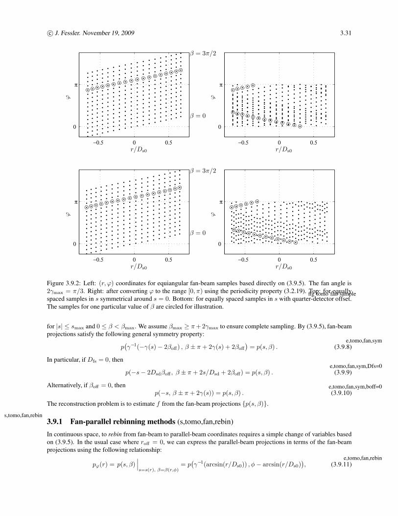
3.9.1 Fan-parallel rebinning methods (s,tomo,fan,rebin) . . . . . . . . . . . . . . . . . . . . . 3.31
3.9.2 The filter-backproject (FBP) approach for 360◦ scans (s,tomo,fan,fbp) . . . . . . . . . . . 3.32
3.1
Page 2
c© J. Fessler. November 19, 2009 3.2
3.9.2.1 Equiangular case . . . . . . . . . . . . . . . . . . . . . . . . . . . . . . . . . 3.33
3.9.2.2 Equidistant case . . . . . . . . . . . . . . . . . . . . . . . . . . . . . . . . . 3.34
3.9.3 FBP for short scans (s,tomo,fan,short) . . . . . . . . . . . . . . . . . . . . . . . . . . . 3.34
3.9.4 The backproject-filter (BPF) approach (s,tomo,fan,bpf) . . . . . . . . . . . . . . . . . . . 3.35
3.9.5 Cone-beam reconstruction (s,3d,cone) . . . . . . . . . . . . . . . . . . . . . . . . . . . 3.36
3.9.5.1 Equidistant case (flat detector) . . . . . . . . . . . . . . . . . . . . . . . . . . 3.36
3.9.5.2 Equiangular case (3rd generation multi-slice CT) . . . . . . . . . . . . . . . . 3.37
3.10 Summary (s,tomo,summ) . . . . . . . . . . . . . . . . . . . . . . . . . . . . . . . . . . . . . . 3.38
3.11 Problems (s,tomo,prob) . . . . . . . . . . . . . . . . . . . . . . . . . . . . . . . . . . . . . . . 3.38
3.1 Introduction (s,tomo,intro)s,tomo,intro
The primary focus of this book is on statistical methods for tomographic image reconstruction using reasonably re-
alistic physical models. Nevertheless, analytical image reconstruction methods, even though based on somewhat
unrealistic simplified models, are important when computation time is so limited that an approximate solution is tol-
erable. Analytical methods are also useful for developing intuition, and for initializing iterative algorithms associated
with statistical reconstruction methods. This chapter reviews classical analytical tomographic reconstruction methods.
(Other names are Fourier reconstruction methods and direct reconstruction methods, because these methods are non-
iterative.) Entire books have been devoted to this subject [2–6], whereas this chapter highlights only a few results.
Many readers will be familiar with much of this material except perhaps for the angularly weighted backprojection
that is described in §3.3. This backprojector is introduced here to facilitate analysis of weighted least-squares (WLS)
formulations in Chapter 4.
There are several limitations of analytical reconstruction methods that impair their performance. Analytical
methods generally ignore measurement noise in the problem formulation and treat noise-related problems as an “af-
terthought” by post-filtering operations. Analytical formulations usually assume continuous measurements and pro-
vide integral-form solutions. Sampling issues are treated by discretizing these solutions “after the fact.” Analytical
methods require certain standard geometries (e.g., parallel rays and complete sampling in radial and angular coordi-
nates). Statistical methods for image reconstruction can overcome all of these limitations.
3.2 Radon transform in 2D (s,tomo,radon)s,tomo,radon
The foundation of analytical reconstruction methods is the Radon transform, which relates a 2D function f(x, y) to
the collection of line integrals of that function. (We focus on the 2D case throughout most of this chapter.) Emission
and transmission tomography systems acquire measurements that are something like blurred line integrals, so the
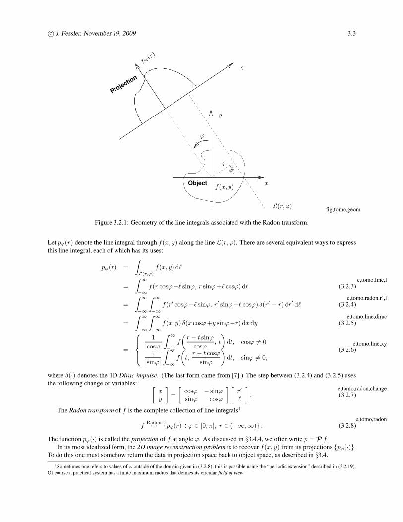
line-integral model represents an idealization of such systems. Fig. 3.2.1 illustrates the geometry of the line integrals
associated with the 2D Radon transform.
3.2.1 Definition
LetL(r, ϕ) denote the line in the Euclidean plane at angle ϕ counter-clockwise from the y axis and at a signed distance
r from the origin:
L(r, ϕ) ={(x, y) ∈ R
2: x cosϕ+y sinϕ = r
}(3.2.1)
= {(r cosϕ−ℓ sinϕ, r sinϕ+ℓ cosϕ) : ℓ ∈ R} . (3.2.2)e,tomo,ray
Page 3
c© J. Fessler. November 19, 2009 3.3
Projectio
n
Objectf(x, y)
L(r, ϕ)
pϕ(r)
r
r
x
y
ϕ
ϕ
Figure 3.2.1: Geometry of the line integrals associated with the Radon transform.
fig,tomo,geom
Let pϕ(r) denote the line integral through f(x, y) along the line L(r, ϕ). There are several equivalent ways to express
this line integral, each of which has its uses:
pϕ(r) =
∫
L(r,ϕ)
f(x, y) dℓ
=
∫ ∞
−∞f(r cosϕ−ℓ sinϕ, r sinϕ+ℓ cosϕ) dℓ (3.2.3)
e,tomo,line,l
=
∫ ∞
−∞
∫ ∞
−∞f(r′ cosϕ−ℓ sinϕ, r′ sinϕ+ℓ cosϕ) δ(r′ − r) dr′ dℓ (3.2.4)
e,tomo,radon,r’,l
=
∫ ∞
−∞
∫ ∞
−∞f(x, y) δ(x cosϕ+y sinϕ−r) dxdy (3.2.5)
e,tomo,line,dirac
=
1
|cosϕ|
∫ ∞
−∞f
(r − t sinϕ
cosϕ, t
)
dt, cosϕ 6= 0
1
|sinϕ|
∫ ∞
−∞f
(
t,r − t cosϕ
sinϕ
)
dt, sinϕ 6= 0,(3.2.6)
e,tomo,line,xy
where δ(·) denotes the 1D Dirac impulse. (The last form came from [7].) The step between (3.2.4) and (3.2.5) uses
the following change of variables:[
xy
]
=
[cosϕ − sinϕsinϕ cosϕ
] [r′
ℓ
]
. (3.2.7)e,tomo,radon,change
The Radon transform of f is the complete collection of line integrals1
fRadon↔ {pϕ(r) : ϕ ∈ [0, π], r ∈ (−∞,∞)} . (3.2.8)
e,tomo,radon
The function pϕ(·) is called the projection of f at angle ϕ. As discussed in §3.4.4, we often write p = P f .
In its most idealized form, the 2D image reconstruction problem is to recover f(x, y) from its projections {pϕ(·)}.To do this one must somehow return the data in projection space back to object space, as described in §3.4.
1Sometimes one refers to values of ϕ outside of the domain given in (3.2.8); this is possible using the “periodic extension” described in (3.2.19).
Of course a practical system has a finite maximum radius that defines its circular field of view.
Page 4
c© J. Fessler. November 19, 2009 3.4
x,tomo,proj,disk Example 3.2.1 Consider the centered uniform disk object with radius r0:
f(x, y) = α rect
(r
2r0
)
, rect(t) , 1{|t|≤1/2} =
{1, |t| ≤ 1/20, otherwise.
(3.2.9)e,rect
Using (3.2.3), the Radon transform of this object is:
pϕ(r) =
∫ ∞
−∞f(r cosϕ−ℓ sinϕ, r sinϕ+ℓ cosϕ) dℓ
=
∫ ∞
−∞α rect
(√
(r cosϕ−ℓ sinϕ)2 + (r sinϕ +ℓ cosϕ)2
2r0
)
dℓ
= α
∫ ∞
−∞rect
(√r2 + ℓ2
2r0
)
dℓ = α
∫
{ℓ : r2+ℓ2≤r20}
dℓ = α
∫ +√
r20−r2
−√
r20−r2
dℓ
= 2α√
r20 − r2 rect
(r
2r0
)
, (3.2.10)e,tomo,proj,disk
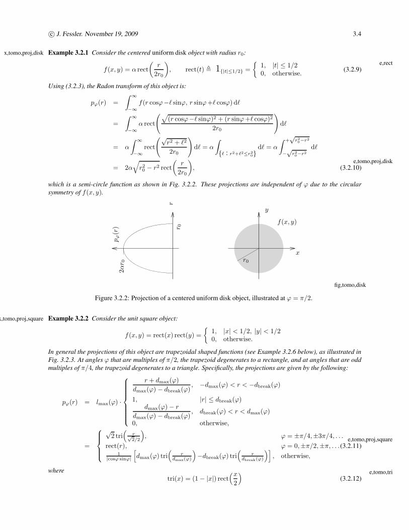
which is a semi-circle function as shown in Fig. 3.2.2. These projections are independent of ϕ due to the circular
symmetry of f(x, y).
f(x, y)
pϕ(r
)
rr 0
r0
2αr 0
x
y
Figure 3.2.2: Projection of a centered uniform disk object, illustrated at ϕ = π/2.
fig,tomo,disk
x,tomo,proj,square Example 3.2.2 Consider the unit square object:
f(x, y) = rect(x) rect(y) =
{1, |x| < 1/2, |y| < 1/20, otherwise.
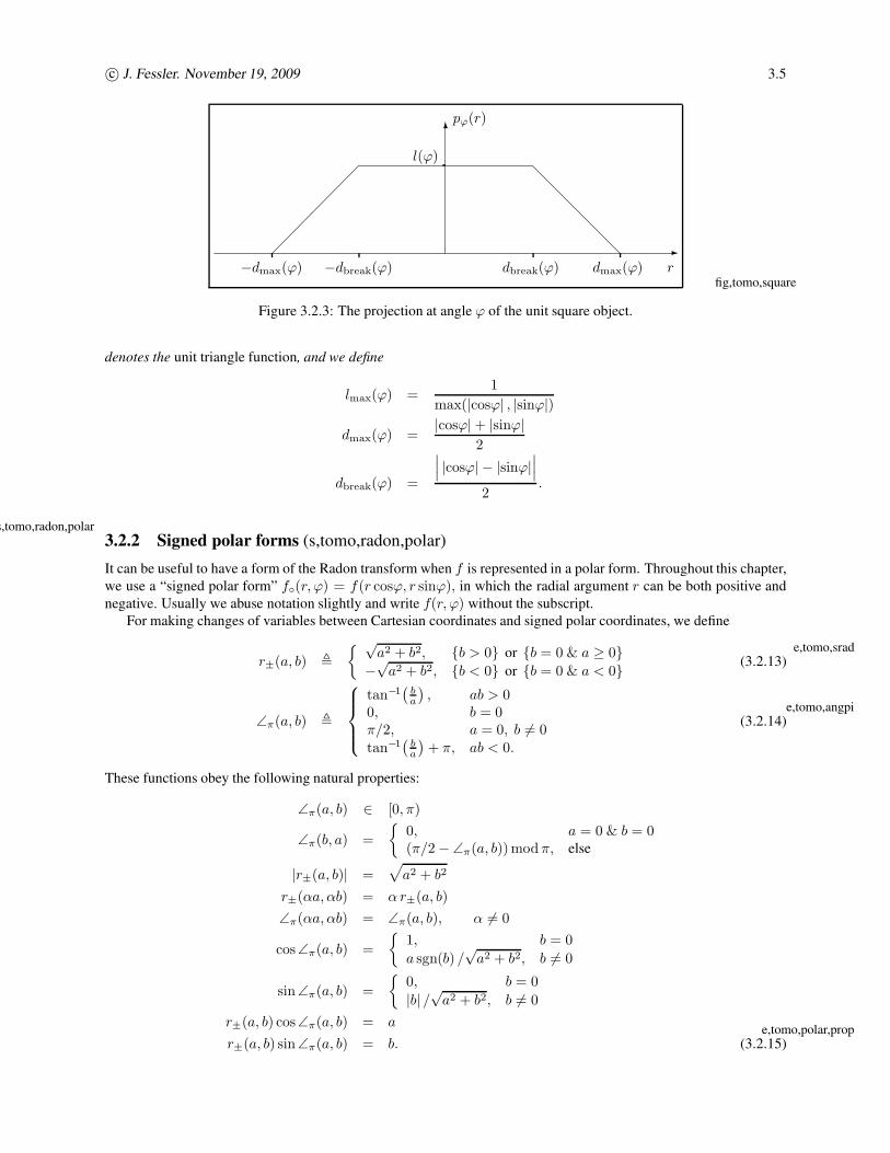
In general the projections of this object are trapezoidal shaped functions (see Example 3.2.6 below), as illustrated in
Fig. 3.2.3. At angles ϕ that are multiples of π/2, the trapezoid degenerates to a rectangle, and at angles that are odd
multiples of π/4, the trapezoid degenerates to a triangle. Specifically, the projections are given by the following:
pϕ(r) = lmax(ϕ) ·
r + dmax(ϕ)
dmax(ϕ) − dbreak(ϕ), −dmax(ϕ) < r < −dbreak(ϕ)
1, |r| ≤ dbreak(ϕ)dmax(ϕ)− r
dmax(ϕ) − dbreak(ϕ), dbreak(ϕ) < r < dmax(ϕ)
0, otherwise,
=
√2 tri
(r√2/2
)
, ϕ = ±π/4,±3π/4, . . .
rect(r), ϕ = 0,±π/2,±π, . . .1
|cosϕ sinϕ|
[
dmax(ϕ) tri(
rdmax(ϕ)
)
−dbreak(ϕ) tri(
rdbreak(ϕ)
)]
, otherwise,
(3.2.11)e,tomo,proj,square
where
tri(x) = (1− |x|) rect(x
2
)
(3.2.12)e,tomo,tri
Page 5
c© J. Fessler. November 19, 2009 3.5
-rdbreak(ϕ)−dbreak(ϕ) dmax(ϕ)−dmax(ϕ)
6pϕ(r)
l(ϕ)
Figure 3.2.3: The projection at angle ϕ of the unit square object.
fig,tomo,square
denotes the unit triangle function, and we define
lmax(ϕ) =1
max(|cosϕ| , |sinϕ|)
dmax(ϕ) =|cosϕ|+ |sinϕ|
2
dbreak(ϕ) =
∣∣∣ |cosϕ| − |sinϕ|
∣∣∣
2.
3.2.2 Signed polar forms (s,tomo,radon,polar)s,tomo,radon,polar
It can be useful to have a form of the Radon transform when f is represented in a polar form. Throughout this chapter,
we use a “signed polar form” f◦(r, ϕ) = f(r cosϕ, r sinϕ), in which the radial argument r can be both positive and
negative. Usually we abuse notation slightly and write f(r, ϕ) without the subscript.
For making changes of variables between Cartesian coordinates and signed polar coordinates, we define
r±(a, b) ,
{ √a2 + b2, {b > 0} or {b = 0 & a ≥ 0}−√
a2 + b2, {b < 0} or {b = 0 & a < 0} (3.2.13)e,tomo,srad
∠π(a, b) ,
tan−1(
ba
), ab > 0
0, b = 0π/2, a = 0, b 6= 0tan−1
(ba
)+ π, ab < 0.
(3.2.14)e,tomo,angpi
These functions obey the following natural properties:
∠π(a, b) ∈ [0, π)
∠π(b, a) =
{0, a = 0 & b = 0(π/2− ∠π(a, b))mod π, else
|r±(a, b)| =√
a2 + b2
r±(αa, αb) = α r±(a, b)
∠π(αa, αb) = ∠π(a, b), α 6= 0
cos∠π(a, b) =
{1, b = 0
a sgn(b) /√
a2 + b2, b 6= 0
sin ∠π(a, b) =
{0, b = 0
|b| /√
a2 + b2, b 6= 0
r±(a, b) cos∠π(a, b) = a
r±(a, b) sin ∠π(a, b) = b. (3.2.15)e,tomo,polar,prop
Page 6
c© J. Fessler. November 19, 2009 3.6
Making a change of variables r = r±(x, y) and ϕ = ∠π(x, y) leads to the following integral relationship:∫ ∞
−∞
∫ ∞
−∞f(x, y) dx dy =
∫ π
0
∫ ∞
−∞f◦(r, ϕ) |r| dr dϕ . (3.2.16)
e,tomo,radon,polar,int
In particular, substituting r′ = r±(x, y) and ϕ′ = ∠π(x, y) into the Radon transform expression (3.2.5) leads to the
following Radon transform in polar coordinates:
pϕ(r) =
∫ π
0
∫ ∞
−∞f◦(r
′, ϕ′) δ(r′ cos(ϕ− ϕ′)−r) |r′| dr′ dϕ′ (3.2.17)e,tomo,line,polar
The properties (3.2.15) arise in several of the subsequent derivations.
3.2.3 Radon transform properties (s,tomo,radon,prop)s,tomo,radon,prop
The following list shows a few of the many properties of the Radon transform. This list is far from exhaustive; indeed
new properties continue to be found, e.g., [8, 9]. Throughout this list, we assume f(x, y)Radon↔ pϕ(r).
• Linearity
If g(x, y)Radon↔ qϕ(r), then
αf + βgRadon↔ αp + βq.
• Shift / translation
f(x− x0, y − y0)Radon↔ pϕ(r − x0 cosϕ−y0 sinϕ) (3.2.18)
e,tomo,radon,shift
• Rotation
f(x cosϕ′ +y sinϕ′,−x sinϕ′ +y cosϕ′)Radon↔ pϕ−ϕ′(r)
• Circular symmetry
f◦(r, ϕ) = f◦(r, 0) ∀ϕ =⇒ pϕ = p0 ∀ϕ
• Symmetry/periodicity
pϕ(r) = pϕ±π(−r) = pϕ±kπ
((−1)kr
), ∀k ∈ Z (3.2.19)
e,tomo,radon,prop,period
• Affine scaling
f(αx, βy)Radon↔
p∠π(β cosϕ, α sinϕ)
(
r|α|β√(β cosϕ)2+(α sinϕ)2
)
√
(β cosϕ)2 + (α sinϕ)2, (3.2.20)
e,tomo,radon,prop,affine
for α, β 6= 0, where r± and ∠π were defined in §3.2.2.
The following two properties are special cases of the affine scaling property.
• Magnification/minification
f(αx, αy)Radon↔ 1
|α| pϕ(αr), α 6= 0
• Flips
f(x,−y)Radon↔ pπ−ϕ(−r)
f(−x, y)Radon↔ pπ−ϕ(r)
• The projection integral theorem
For a scalar function h : R→ R:∫
pϕ(r) h(r) dr =
∫ (∫
f(r cosϕ−ℓ sinϕ, r sinϕ+ℓ cosϕ) dℓ
)
h(r) dr
=
∫∫
f(x, y)h(x cosϕ+y sinϕ) dx dy, (3.2.21)e,tomo,pit
by making the orthonormal coordinate rotation: x = r cosϕ−ℓ sinϕ, y = r sinϕ+ℓ cosϕ .
Page 7
c© J. Fessler. November 19, 2009 3.7
>
^
x
y >
v
π/2
π
0 0 r
ϕ
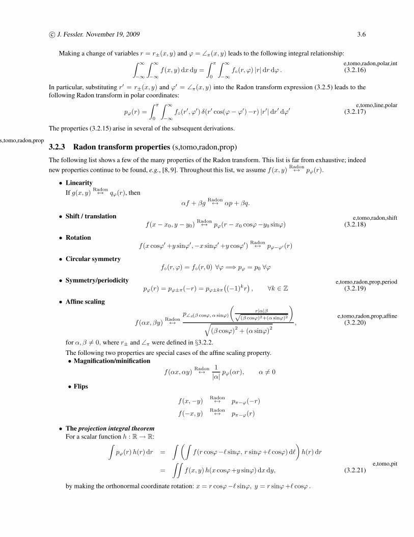
Figure 3.2.4: Left: cross-section of 2D object containing three Dirac impulses. Right: the corresponding sinogram
consisting of three sinusoidal impulse ridges.
fig˙tomo˙sino˙points
• Volume conservation ∫ ∞
−∞
∫ ∞
−∞f(x, y) dx dy =
∫ ∞
−∞pϕ(r) dr, ∀ϕ. (3.2.22)
e,tomo,radon,dc
This is a corollary to the projection integral theorem for h(r) = 1. The volume conservation property is one of
many consistency conditions of the Radon transform [4].
The following example serves to illustrate some of these properties.
x,tomo,proj,dirac Example 3.2.3 Consider the object f(x, y) = δ2(x − x0, y − y0), the 2D Dirac impulse centered at (x0, y0). This
generalized function can be thought of as a disk function centered at (x0, y0) of radius r0 and height 1/(πr20) (so that
volume is unity) in the limit as r0 → 0.
Let Cr0(r) = 2
√
r20 − r2 rect
(r
2r0
)
denote the projection of centered uniform disk with radius r0 as derived in
(3.2.10) in Example 3.2.1. Then by the shift property (3.2.18), the projections of a disk centered at (x0, y0) are:
pϕ(r) = Cr0(r − [x0 cosϕ+y0 sinϕ]).
(See Fig. 3.2.5 below.) Thus the projections of the 2D Dirac impulse are found as follows:
pϕ(r) =1
πr20
Cr0(r − [x0 cosϕ+y0 sinϕ])→ δ(r − [x0 cosϕ+y0 sinϕ]) as r0 → 0.
In summary, for a 2D Dirac impulse object located at (x0, y0), the projection at angle ϕ is a 1D Dirac impulse located
at r = x0 cosϕ +y0 sinϕ. See Fig. 3.2.4.
3.2.4 Sinogram
Because pϕ(r) is a function of two arguments, we can display pϕ(r) as a 2D grayscale picture where usually r and ϕare the horizontal and vertical axes respectively. If we make such a display of the projections pϕ(r) of a Dirac impulse,
then the picture looks like a sinusoid corresponding to the function r = x0 cosϕ+y0 sinϕ. Hence this 2D function
is called a sinogram and (when sampled) represents the raw data available for image reconstruction. So the goal of
tomographic reconstruction is to estimate the object f(x, y) from a measured sinogram.
Each point (x, y) in object space contributes a unique sinusoid to the sinogram, with the “amplitude” of the sinusoid
being√
x2 + y2, the distance of the point from the origin, and the “phase” of the sinusoid depending on ∠π(x, y).A sinogram is the superposition of all of these sinusoids, each one weighted by the value f(x, y). Hence it seems
plausible that there could be enough information in the sinogram to recover the object f , if we can unscramble all of
those sinusoids.
x,tomo,radon,points Example 3.2.4 Fig. 3.2.4 illustrates these concepts for the object f(x, y) = δ2(x, y)+ δ2(x−1, y)+ δ2(x−1, y−1)with corresponding projections pϕ(r) = δ(r) + δ(r − cosϕ)+ δ(r − cosϕ− sinϕ) .
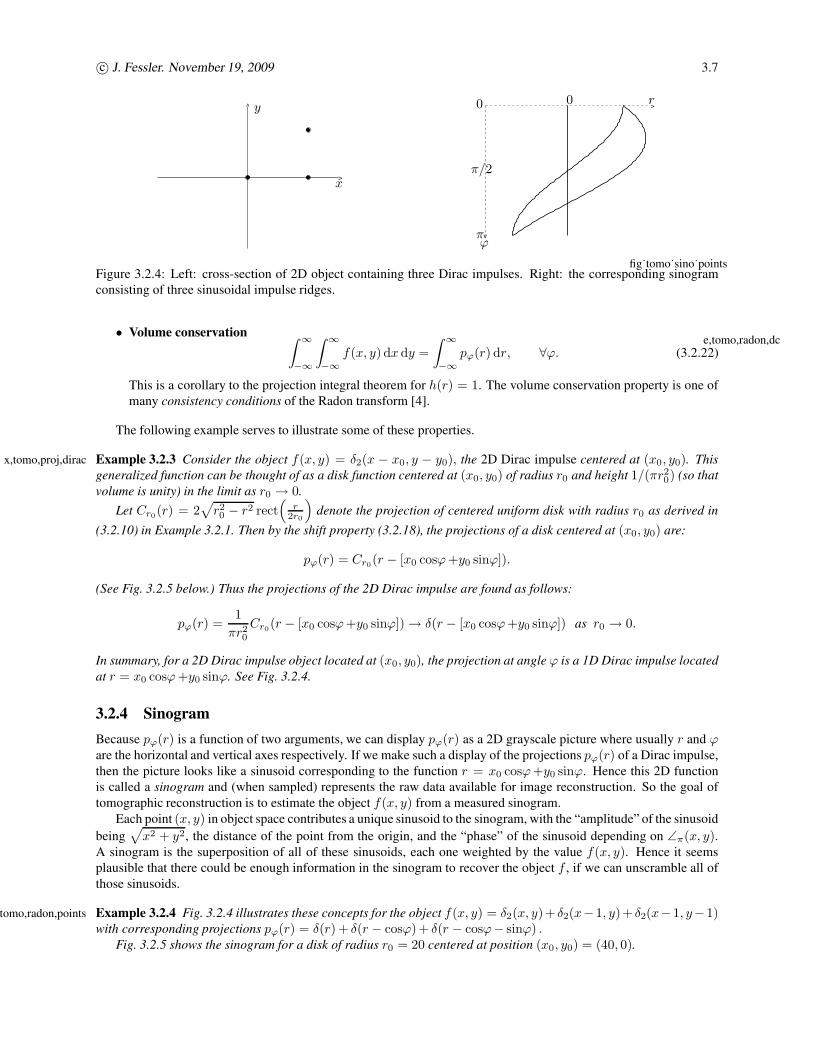
Fig. 3.2.5 shows the sinogram for a disk of radius r0 = 20 centered at position (x0, y0) = (40, 0).
Page 8
c© J. Fessler. November 19, 2009 3.8
Sinogram for Disk
rφ
−60 −40 −20 0 20 40 60
0
179 0
40
Figure 3.2.5: Sinogram for a disk object of radius r0 = 20 centered at (x0, y0) = (40, 0).
fig˙tomo˙disk˙sino
3.2.5 Fourier-slice theorem
The most important corollary of the projection-integral theorem (3.2.21) is the Fourier-slice theorem, also known
as the central-slice theorem or central-section theorem or projection-slice theorem. In words, the statement of this
theorem is as follows2. If pϕ(r) denotes the Radon transform of f(x, y), then the 1D Fourier transform of pϕ(·) equals
the slice at angle ϕ through the 2D Fourier transform of f(x, y).Let Pϕ(ν) denote the 1D Fourier transform3 of pϕ(r), i.e.,
Pϕ(ν) =
∫ ∞
−∞pϕ(r) e−ı2πνr dr .
Let F (u, v) denote the 2D Fourier transform of f(x, y), i.e.,
F (u, v) =
∫ ∞
−∞
∫ ∞
−∞f(x, y) e−ı2π(ux+vy) dx dy . (3.2.23)
e,ft2
Then in mathematical notation, the Fourier-slice theorem is simply:
Pϕ(ν) = F (ν cosϕ, ν sinϕ) = F◦(ν, ϕ), ∀ν ∈ R, ∀ϕ ∈ R, (3.2.24)e,tomo,fst
where F◦(ρ, Φ) = F (ρ cosΦ, ρ sinΦ) denotes the polar form of F (u, v). (Again we will frequently recycle notation
and omit the subscript.) The proof of the Fourier-slice theorem is remarkably simple: merely set h(r) = exp(−ı2πνr)in the projection-integral theorem (3.2.21).
It follows immediately from the Fourier-slice theorem that the Radon transform (3.2.8) describes completely any
(Fourier transformable) object f(x, y), because there is a one-to-one correspondence between the Radon transform
and the 2D Fourier transform F (u, v), and from F (u, v) we can recover f(x, y) by an inverse 2D Fourier transform.
x,tomo,slice,bessel Example 3.2.5 For the circularly symmetric Bessel object f(x, y) = f(r) = (π/2)J0(πr), from a table of Hankel
transforms F (ρ) = 12 δ(|ρ| − 1
2
). (So F (ρ) is an impulse-ring of radius 1/2.) Thus Pϕ(ν) = F (ν) = 1
2 δ(|ν| − 1
2
)=
12 δ(ν − 1
2
)+ 1
2 δ(ν + 1
2
), so pϕ(r) = cos(πr) . So the projections of Bessel objects are sinusoids.
x,tomo,slice,rect Example 3.2.6 The 2D the uniform rectangle object and its Fourier transform are
f(x, y) = rect(x
a
)
rect(y
b
)2D FT←→ F (u, v) = a sinc(au) b sinc(bv),
2Apparently the first publication of this result was in Bracewell’s 1956 paper [10]. However, at a symposium on 2004-7-17 held at Stanford
University to celebrate the 75th birthday of Albert Macovski, Ron Bracewell stated that he believes that the theorem was “well known” to other
radio astronomers at the time.3Being an engineer, I simply assume existence of the Fourier transforms of all functions of interest here.
Page 9
c© J. Fessler. November 19, 2009 3.9
so in polar form: F◦(ρ, Φ) = a sinc(aρ cosΦ) b sinc(bρ sinΦ) . By the Fourier slice theorem, the 1D FT of its projec-
tions are given by
Pϕ(ν) = F◦(ν, ϕ) = a sinc(νa cosϕ) b sinc(νb sinϕ) . (3.2.25)e,tomo,slice,rect,Pau
Thus, by the convolution property of the FT (27.3.3), each projection is the convolution of two rect functions:
pϕ(r) =1
|cosϕ| rect(
r
a cosϕ
)
∗ 1
|sinϕ| rect(
r
b sinϕ
)
, (3.2.26)e,tomo,slice,rect,proj
which is a trapezoid in general, as illustrated Fig. 3.2.3 for the case a = b = 1. (The “∗” above denotes 1D
convolution with respect to r.)
s,tomo,proj,disk Example 3.2.7 The 2D FT of a uniform disk object f(x, y) = rect(
r2r0
)
is F (ρ) = r20 jinc(r0ρ).
Thus Pϕ(ν) = r20 jinc(r0ν) = r2
0J1(πr0ν)
2r0ν , where J1 denotes the 1st-order Bessel function of the first kind. Because
J1(2πν)/(2ν) and√
1− t2 rect(t/2) are 1D Fourier transform pairs [11, p. 337], we see that the projections of a
uniform disk are given by pϕ(r) = 2√
r20 − r2 rect
(r
2r0
)
. This agrees with the result shown in (3.2.10) by integration.
x,tomo,slice,gauss Example 3.2.8 Consider the 2D gaussian object f(x, y) = f(r) = 1w2 exp
(
−π(
rw
)2)
, with corresponding 2D FT
F (ρ) = exp(−π(wρ)2
). By the Fourier-slice theorem: Pϕ(ν) = exp
(−π(wν)2
), the inverse 1D Fourier transform
of which is pϕ(r) = 1w exp
(
−π(
rw
)2)
. (Notice the slight change in the leading constant.) Thus the projections of a
gaussian object are gaussian, which is a particularly important relationship. In fact, this property is related to the fact
that two jointly gaussian random variables have gaussian marginal distributions.
The following corollary follows directly from the Fourier-slice theorem.
c,tomo,radon,conv Corollary 3.2.9 (Convolution property.) If fRadon↔ p and g
Radon↔ q then
f(x, y) ∗∗ g(x, y)Radon↔ pϕ(r) ∗ qϕ(r) . (3.2.27)
e,tomo,radon,conv
In particular, it follows from Example 3.2.8 that 2D gaussian smoothing of an object is equivalent to 1D radial gaussian
smoothing of each projection4:
f(x, y) ∗∗ 1
w2e−π(r/w)2 Radon↔ pϕ(r) ∗ 1
we−π(r/w)2 .
3.3 Backprojection (s,tomo,back)s,tomo,back
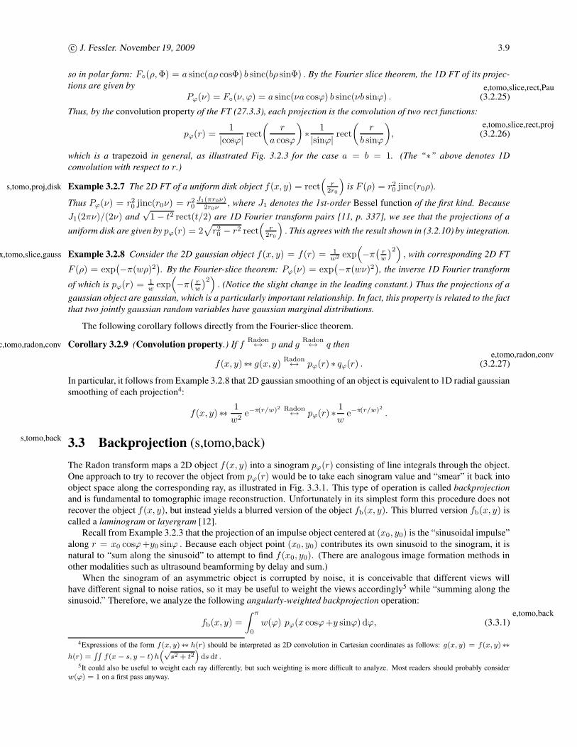
The Radon transform maps a 2D object f(x, y) into a sinogram pϕ(r) consisting of line integrals through the object.
One approach to try to recover the object from pϕ(r) would be to take each sinogram value and “smear” it back into
object space along the corresponding ray, as illustrated in Fig. 3.3.1. This type of operation is called backprojection
and is fundamental to tomographic image reconstruction. Unfortunately in its simplest form this procedure does not
recover the object f(x, y), but instead yields a blurred version of the object fb(x, y). This blurred version fb(x, y) is
called a laminogram or layergram [12].
Recall from Example 3.2.3 that the projection of an impulse object centered at (x0, y0) is the “sinusoidal impulse”
along r = x0 cosϕ+y0 sinϕ . Because each object point (x0, y0) contributes its own sinusoid to the sinogram, it is
natural to “sum along the sinusoid” to attempt to find f(x0, y0). (There are analogous image formation methods in
other modalities such as ultrasound beamforming by delay and sum.)
When the sinogram of an asymmetric object is corrupted by noise, it is conceivable that different views will
have different signal to noise ratios, so it may be useful to weight the views accordingly5 while “summing along the
sinusoid.” Therefore, we analyze the following angularly-weighted backprojection operation:
fb(x, y) =
∫ π
0
w(ϕ) pϕ(x cosϕ+y sinϕ) dϕ, (3.3.1)e,tomo,back
4Expressions of the form f(x, y) ∗∗ h(r) should be interpreted as 2D convolution in Cartesian coordinates as follows: g(x, y) = f(x, y) ∗∗h(r) =
RR
f(x − s, y − t) h“√
s2 + t2”
ds dt .5It could also be useful to weight each ray differently, but such weighting is more difficult to analyze. Most readers should probably consider
w(ϕ) = 1 on a first pass anyway.
Page 10
c© J. Fessler. November 19, 2009 3.10
Projectio
n
L(r, ϕ)
pϕ(r)
r
r
ϕ
x
y
Figure 3.3.1: Illustration of back projection operation for a single projection view.
fig,tomo,back
where w(ϕ) denotes the user-chosen weight for angle ϕ. In the usual case where w(ϕ) = 1, this operation is the
adjoint of the Radon transform (see §3.4.4).
3.3.1 Image-domain analysis
The following theorem shows that the laminogram fb(x, y) is a severely blurred version of the original object f(x, y).
t,tomo,1/r Theorem 3.3.1 If pϕ(r) denotes the Radon transform of f(x, y) as given by (3.2.3), and fb(x, y) denotes the angularly-
weighted backprojection of pϕ(r) as given by (3.3.1), then
fb(x, y) = h(r, ϕ) ∗∗ f(x, y), where h(r, ϕ) =w((ϕ + π/2)modπ)
|r| , (3.3.2)e,tomo,1r
for ϕ ∈ [0, π] and r ∈ R.
Proof:
It is clear from (3.2.3) and (3.3.1) that the operation f(x, y)→ pϕ(r)→ fb(x, y) is linear. Furthermore, this operation
is shift invariant because
fb(x− c, y − d) =
∫ π
0
w(ϕ) pϕ((x− c) cosϕ+(y − d) sinϕ) dϕ
=
∫ π
0
w(ϕ) qϕ(x cosϕ+y sinϕ) dϕ,
where, using the shift property (3.2.18), the projections qϕ(r) , pϕ(r − c cosϕ−d sinϕ) denote the Radon transform
of f(x− c, y − d).
Page 11
c© J. Fessler. November 19, 2009 3.11
Due to this shift-invariance, it suffices to examine the behavior of fb(x, y) at a single location, such as the center.
Using (3.2.3):
fb(0, 0) =
∫ π
0
w(ϕ′) pϕ′(0) dϕ′
=
∫ π
0
w(ϕ′)
[∫ ∞
−∞f(0 cosϕ′−ℓ sinϕ′, 0 sinϕ′ +ℓ cosϕ′) dℓ
]
dϕ′
=
∫ π
0
∫ ∞
−∞
w((ϕ + π/2)modπ)
|r| f(0− r cosϕ, 0− r sinϕ) |r| dr dϕ, (3.3.3)e,tomo,back,b00
making the variable changes ϕ′ = (ϕ+π/2)modπ and ℓ =
{r, ϕ′ ∈ [π/2, π]−r, ϕ′ ∈ [0, π/2).
Thus, using the shift-invariance
property noted above:
fb(x, y) =
∫ π
0
∫ ∞
−∞
w((ϕ + π/2)modπ)
|r| f(x− r cosϕ, y − r sinϕ) |r| dr dϕ, (3.3.4)e,tomo,back,bxy,proof
which is the convolution integral (3.3.2) in (signed) polar coordinates. 2
An alternative proof uses the projection and backprojection of a centered Dirac impulse based on Example 3.2.3.
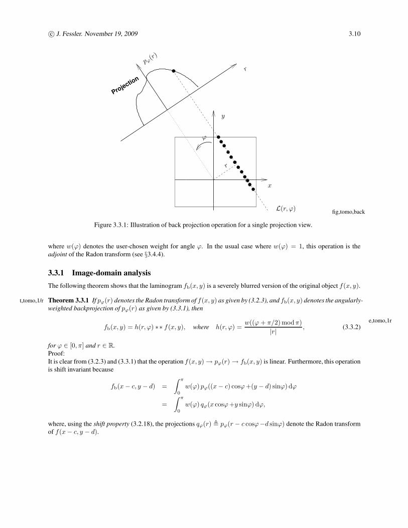
In the usual case where w(ϕ) = 1, we see from (3.3.2) that unmodified backprojection yields a result that is the
original object blurred by the 1/r function. This PSF has very heavy tails, so the laminogram is nearly useless for
visual interpretation. Fig. 3.3.2 illustrates the 1/r function.
Thus far we have focused on the parallel ray geometry implicit in (3.2.3). For a broad family of other geometries,
Gullberg and Zeng [13] found appropriate pixel-dependent weighted-backprojection operations that also yield the
original object convolved with 1/r. So the nature of (3.3.2) is fairly general.
h(r)
x
y
−5 −4 −3 −2 −1 0 1 2 3 4 5
−5
−4
−3
−2
−1
0
1
2
3
4
5
0
1
2
3
4
5
6
7
8
9
10
−5
0
5
−5
0
50
50
100
150
200
250
300
xy
Figure 3.3.2: Illustrations of 1/r function and its “heavy tails.”
fig˙tomo˙1r˙grayfig˙tomo˙1r˙surf
3.3.2 Frequency-domain analysis
Because the laminogram fb(x, y) is the object f(x, y) convolved with the PSF h(r, ϕ) in (3.3.2), it follows that in the
frequency domain we have
Fb(ρ, Φ) = H(ρ, Φ)F◦(ρ, Φ),
where H(ρ, Φ) denotes the polar form of the 2D FT of h(r, ϕ).It is well known that 1/ |r| and 1/ |ρ| are 2D FT pairs [11, p. 338]. The following theorem generalizes that result
to the angularly weighted case.
Page 12
c© J. Fessler. November 19, 2009 3.12
t,tomo,2dft,1r Theorem 3.3.2 The PSF given in (3.3.2) has the following 2DFT for6 Φ ∈ [0, π] and ρ ∈ R:
h(r, ϕ) =1
|r| w((ϕ + π/2)modπ)2D FT←→ H(ρ, Φ) =
1
|ρ| w(Φ) . (3.3.5)e,tomo,2dft,1r
Proof:
Evaluate the 2D FT of h:
H(ρ, Φ) =
∫ π
0
∫ ∞
−∞h(r, ϕ) e−ı2πrρ cos(ϕ−Φ) |r| dr dϕ
=
∫ π
0
w((ϕ + π/2)mod π)
[∫ ∞
−∞e−ı2πrρ cos(ϕ−Φ) dr
]
dϕ
=
∫ π
0
w((ϕ + π/2)mod π) δ(ρ cos(ϕ− Φ)) dϕ
=1
|ρ|
∫ π
0
w(ϕ′) δ(sin(ϕ′ − Φ)) dϕ′ =1
|ρ| w(Φ),
letting ϕ′ = (ϕ + π/2)mod π and using7 the following Dirac impulse property [11, p. 100]
δ(f(t)) =∑
s : f(s)=0
δ(t− s)∣∣∣f(s)
∣∣∣
. (3.3.6)e,tomo,back,dirac
In particular,
δ(sin(t)) =∑
k
δ(t + πk) .
Thus, the 2D FT of h(r, ϕ) in (3.3.2) is H(ρ, Φ) = w(Φ) / |ρ|. 2
So the frequency-space relationship between the laminogram and the original object is
Fb(ρ, Φ) =w(Φ)
|ρ| F◦(ρ, Φ) . (3.3.7)e,tomo,lamino,1rho
High spatial frequencies are severely attenuated by the 1/ |ρ| term, so the laminogram is very blurry. However, the
relationship (3.3.7) immediately suggests a “deconvolution” method for recovering f(x, y) from fb(x, y), as described
in the next section.
More generally, if qϕ(r) is an arbitrary sinogram to which we apply a weighted backprojection of the form (3.3.1),
then the Fourier transform of the resulting image is
Fb(ρ, Φ) =w(Φ)
|ρ| Qϕ(ν)∣∣∣ν=ρ, ϕ=Φ
=w(Φ)
|ρ|
{QΦ(ρ), Φ ∈ [0, π)QΦ−π(−ρ), Φ ∈ [π, 2π),
(3.3.8)e,tomo,back,general
where Qϕ(ν) is the 1D FT of qϕ(r) along r. (See Problem 3.15.) The special case (3.3.7) follows from the Fourier-
slice theorem.
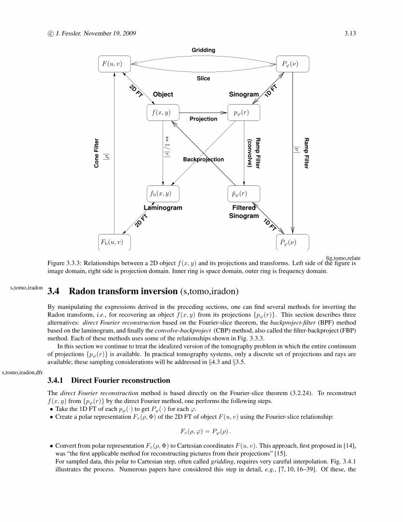
Summary
Fig. 3.3.3 summarizes the various Fourier-transform relationships described above, as well as the Fourier-slice theo-
rem, and the projection and backprojection operations.
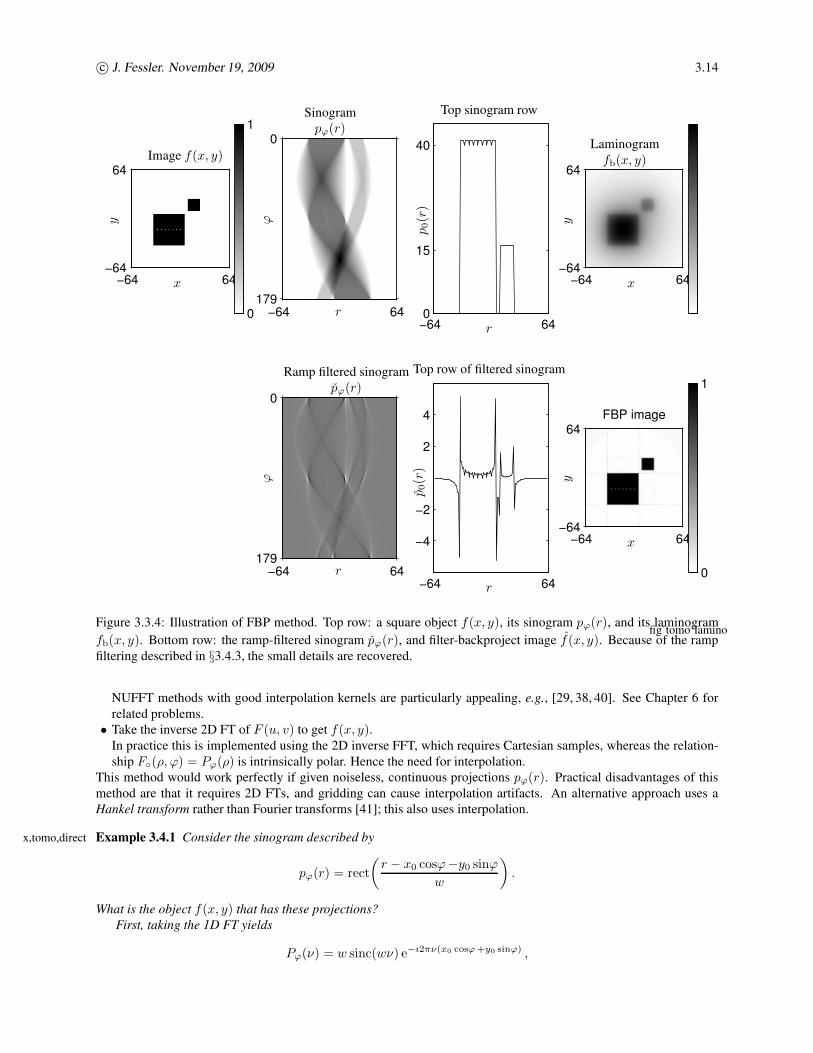
x,tomo,back Example 3.3.3 Fig. 3.3.4 shows an object f(x, y) consisting of two squares, the larger of which has several small
holes in it. Also shown is the sinogram pϕ(r) of this object. The laminogram fb(x, y) is so severely blurred that the
small holes are not visible.
6Alternatively we could write H(ρ, Φ) = 1
|ρ|w(Φ mod π) for Φ ∈ [0, 2π) and ρ ≥ 0.
7Some readers may question the rigor of this proof, and well they should because the function 1/ |r| is not square integrable so the existence of
its 2D FT is questionable. Apparently this transform pair belongs in the family that includes Dirac impulses, sinusoids, step functions, etc.
Page 13
c© J. Fessler. November 19, 2009 3.13
Object
Projection
Backprojection
Sinogram
Sinogram
FilteredLaminogram
2D F
T 1D FT
2D FT 1D
FT
Gridding
Ra
mp
Filte
r
(co
nv
olv
e)
Ra
mp
Filte
rCo
ne
Fil
ter
Slice
f(x, y)
fb(x, y)
pϕ(r)
pϕ(r)
F (u, v)
Fb(u, v)
Pϕ(ν)
Pϕ(ν)∗∗
1/|r|
|ν||ρ|
Figure 3.3.3: Relationships between a 2D object f(x, y) and its projections and transforms. Left side of the figure is
image domain, right side is projection domain. Inner ring is space domain, outer ring is frequency domain.
fig,tomo,relate
3.4 Radon transform inversion (s,tomo,iradon)s,tomo,iradon
By manipulating the expressions derived in the preceding sections, one can find several methods for inverting the
Radon transform, i.e., for recovering an object f(x, y) from its projections {pϕ(r)}. This section describes three
alternatives: direct Fourier reconstruction based on the Fourier-slice theorem, the backproject-filter (BPF) method
based on the laminogram, and finally the convolve-backproject (CBP) method, also called the filter-backproject (FBP)
method. Each of these methods uses some of the relationships shown in Fig. 3.3.3.
In this section we continue to treat the idealized version of the tomography problem in which the entire continuum
of projections {pϕ(r)} is available. In practical tomography systems, only a discrete set of projections and rays are
available; these sampling considerations will be addressed in §4.3 and §3.5.
3.4.1 Direct Fourier reconstructions,tomo,iradon,dfr
The direct Fourier reconstruction method is based directly on the Fourier-slice theorem (3.2.24). To reconstruct
f(x, y) from {pϕ(r)} by the direct Fourier method, one performs the following steps.
• Take the 1D FT of each pϕ(·) to get Pϕ(·) for each ϕ.
• Create a polar representation F◦(ρ, Φ) of the 2D FT of object F (u, v) using the Fourier-slice relationship:
F◦(ρ, ϕ) = Pϕ(ρ) .
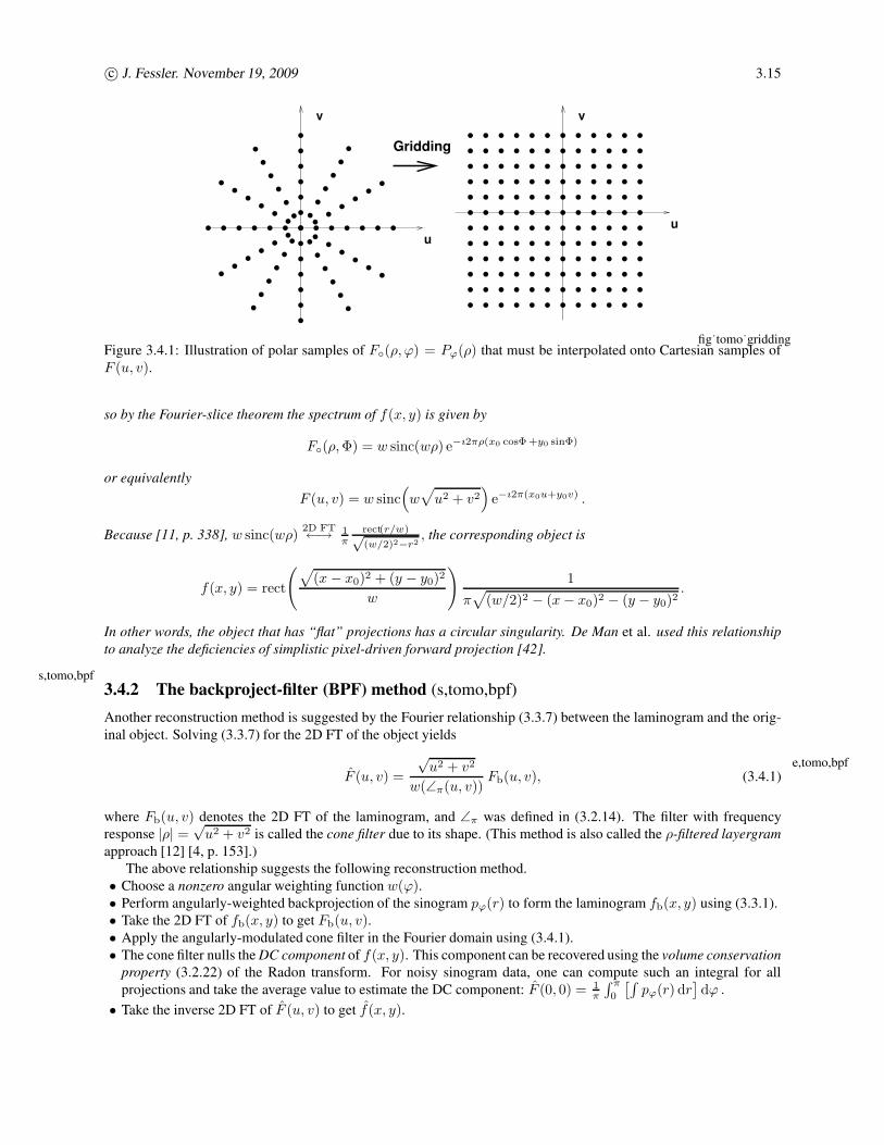
• Convert from polar representation F◦(ρ, Φ) to Cartesian coordinates F (u, v). This approach, first proposed in [14],
was “the first applicable method for reconstructing pictures from their projections” [15].
For sampled data, this polar to Cartesian step, often called gridding, requires very careful interpolation. Fig. 3.4.1
illustrates the process. Numerous papers have considered this step in detail, e.g., [7, 10, 16–39]. Of these, the
Page 14
c© J. Fessler. November 19, 2009 3.14
−64 64−64
64
0
1
−64 64
0
179
−64 640
15
40
−64 64−64
64
−64 64
0
179
−64 64
−4
−2
2
4 FBP image
−64 64−64
64
0
1
x
xx
yyy
r
r
r
r
ϕϕ
p0(r
)p0(r
)
Image f(x, y)Laminogram
fb(x, y)
Sinogram
pϕ(r)
Ramp filtered sinogram
pϕ(r)
Top sinogram row
Top row of filtered sinogram
Figure 3.3.4: Illustration of FBP method. Top row: a square object f(x, y), its sinogram pϕ(r), and its laminogram
fb(x, y). Bottom row: the ramp-filtered sinogram pϕ(r), and filter-backproject image f(x, y). Because of the ramp
filtering described in §3.4.3, the small details are recovered.
fig˙tomo˙lamino
NUFFT methods with good interpolation kernels are particularly appealing, e.g., [29, 38, 40]. See Chapter 6 for
related problems.
• Take the inverse 2D FT of F (u, v) to get f(x, y).In practice this is implemented using the 2D inverse FFT, which requires Cartesian samples, whereas the relation-
ship F◦(ρ, ϕ) = Pϕ(ρ) is intrinsically polar. Hence the need for interpolation.
This method would work perfectly if given noiseless, continuous projections pϕ(r). Practical disadvantages of this
method are that it requires 2D FTs, and gridding can cause interpolation artifacts. An alternative approach uses a
Hankel transform rather than Fourier transforms [41]; this also uses interpolation.
x,tomo,direct Example 3.4.1 Consider the sinogram described by
pϕ(r) = rect
(r − x0 cosϕ−y0 sinϕ
w
)
.
What is the object f(x, y) that has these projections?
First, taking the 1D FT yields
Pϕ(ν) = w sinc(wν) e−ı2πν(x0 cosϕ +y0 sinϕ) ,
Page 15
c© J. Fessler. November 19, 2009 3.15
v
Gridding
v
u
u
Figure 3.4.1: Illustration of polar samples of F◦(ρ, ϕ) = Pϕ(ρ) that must be interpolated onto Cartesian samples of
F (u, v).
fig˙tomo˙gridding
so by the Fourier-slice theorem the spectrum of f(x, y) is given by
F◦(ρ, Φ) = w sinc(wρ) e−ı2πρ(x0 cosΦ +y0 sinΦ)
or equivalently
F (u, v) = w sinc(
w√
u2 + v2)
e−ı2π(x0u+y0v) .
Because [11, p. 338], w sinc(wρ)2D FT←→ 1
πrect(r/w)√(w/2)2−r2
, the corresponding object is
f(x, y) = rect
(√
(x − x0)2 + (y − y0)2
w
)
1
π√
(w/2)2 − (x− x0)2 − (y − y0)2.
In other words, the object that has “flat” projections has a circular singularity. De Man et al. used this relationship
to analyze the deficiencies of simplistic pixel-driven forward projection [42].
3.4.2 The backproject-filter (BPF) method (s,tomo,bpf)s,tomo,bpf
Another reconstruction method is suggested by the Fourier relationship (3.3.7) between the laminogram and the orig-
inal object. Solving (3.3.7) for the 2D FT of the object yields
F (u, v) =
√u2 + v2
w(∠π(u, v))Fb(u, v), (3.4.1)
e,tomo,bpf
where Fb(u, v) denotes the 2D FT of the laminogram, and ∠π was defined in (3.2.14). The filter with frequency
response |ρ| =√
u2 + v2 is called the cone filter due to its shape. (This method is also called the ρ-filtered layergram
approach [12] [4, p. 153].)
The above relationship suggests the following reconstruction method.
• Choose a nonzero angular weighting function w(ϕ).• Perform angularly-weighted backprojection of the sinogram pϕ(r) to form the laminogram fb(x, y) using (3.3.1).
• Take the 2D FT of fb(x, y) to get Fb(u, v).• Apply the angularly-modulated cone filter in the Fourier domain using (3.4.1).
• The cone filter nulls the DC component of f(x, y). This component can be recovered using the volume conservation
property (3.2.22) of the Radon transform. For noisy sinogram data, one can compute such an integral for all
projections and take the average value to estimate the DC component: F (0, 0) = 1π
∫ π
0
[∫pϕ(r) dr
]dϕ .
• Take the inverse 2D FT of F (u, v) to get f(x, y).
Page 16
c© J. Fessler. November 19, 2009 3.16
This approach is called the backproject-filter (BPF) method because we first backproject the sinograms, and then apply
the cone filter to “deconvolve” the 1/ |ρ| effect of the backprojection.
In practice, using the cone-filter without modification would excessively amplify high-frequency noise. To control
noise, the cone-filter is usually apodized in the frequency domain with a windowing function. Specifically, we replace
(3.4.1) by
F (u, v) = A(u, v)
√u2 + v2
w(∠π(u, v))Fb(u, v),
where A(u, v) is an apodizing lowpass filter. In the absence of noise, the resulting reconstructed image satisfies
f(x, y) = a(x, y) ∗∗ f(x, y),
where a(x, y) is the inverse 2D FT of A(u, v). (See [43, 44] for early 3D versions of BPF.)
One practical difficulty with the BPF reconstruction method is that the laminogram fb(x, y) has unbounded spatial
support (even for a finite-support object f ) due to the tails of the 1/ |r| response in (3.3.2). In practice the support of
fb(x, y) must be truncated to a finite size for computer storage, and such truncation of tails can cause problems with
the deconvolution step. Furthermore, using 2D FFTs to apply the cone filter results in periodic convolution which can
cause wrap-around effects due to the high-pass nature of the cone filter. To minimize artifacts due to spatial truncation
and periodic convolution, one must evaluate fb(x, y) numerically onto a support grid that is considerably larger than
the support of the object f(x, y). A large support increases the computational costs of both the backprojection step
and the 2D FFT operations used for the cone filter. The FBP reconstruction method, described next, largely overcomes
this limitation. The FBP method has the added benefit of only requiring 1D Fourier transforms, whereas the direct
Fourier and BPF methods require 2D transforms.
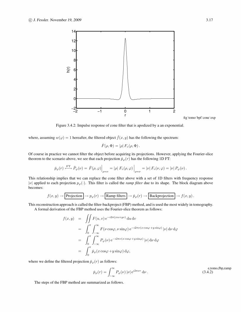
x,tomo,bpf,cone,exp Example 3.4.2 For theoretical analysis, a convenient choice for the apodizer is A(ρ) = e−aρ . Using Hankel trans-
forms [11, p. 338] and the Laplacian property (27.3.5):
−4π2r2h(r)Hankel←→ 1
ρ
d
dρH(ρ) +
d2
dρ2 H(ρ),
one can show that that the corresponding impulse response of the apodized cone filter is given by
h(r) = 4πa2 − 2π2r2
(a2 + 4π2r2)5/2
Hankel←→ ρ e−aρ .
Taking the limit as a→ 0 shows that h(r) = −1/(4π2r3) for r 6= 0, and that h(r) has a singularity at r = 0.
Fig. 3.4.2 illustrates this impulse response for the case a = 1.
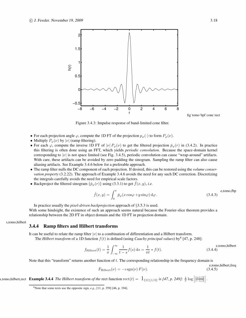
x,tomo,bpf,cone,rect Example 3.4.3 If we band-limit the cone filter by choosing A(ρ) = rect(
ρ2ρmax
)
, then the resulting impulse response
h(r) has a complicated expression that depends on both Bessel functions and the Struve function [45]. Fig. 3.4.3
illustrates this impulse response for the case ρmax = 1.
3.4.3 The filter-backproject (FBP) method (s,tomo,fbp)s,tomo,fbp
We have seen that an unfiltered backprojection yields a blurry laminogram that must be deconvolved by a cone filter
to yield the original image. The steps involved look like the following:
f(x, y)→ Projection → pϕ(r)→ Backprojection︸ ︷︷ ︸
convolution with 1/ |r|
→ fb(x, y)→ Cone filter → f(x, y) .
Because the cascade of the first two operations is linear and shift invariant, as shown in §3.3, in principle we could
move the cone filter to be the first step to obtain the same overall result:
f(x, y)→ Cone filter → f(x, y)→ Projection → pϕ(r)→ Backprojection → f(x, y),
Page 17
c© J. Fessler. November 19, 2009 3.17
−2 −1 0 1 2−2
0
2
4
6
8
10
12
14
r
h(r
)
Figure 3.4.2: Impulse response of cone filter that is apodized by a an exponential.
fig˙tomo˙bpf˙cone˙exp
where, assuming w(ϕ) = 1 hereafter, the filtered object f(x, y) has the following the spectrum:
F (ρ, Φ) = |ρ|F◦(ρ, Φ) .
Of course in practice we cannot filter the object before acquiring its projections. However, applying the Fourier-slice
theorem to the scenario above, we see that each projection pϕ(r) has the following 1D FT:
pϕ(r)FT←→ Pϕ(ν) = F (ρ, ϕ)
∣∣∣ρ=ν
= |ρ| F◦(ρ, ϕ)∣∣∣ρ=ν
= |ν|F◦(ν, ϕ) = |ν|Pϕ(ν) .
This relationship implies that we can replace the cone filter above with a set of 1D filters with frequency response
|ν| applied to each projection pϕ(·). This filter is called the ramp filter due to its shape. The block diagram above
becomes:
f(x, y)→ Projection → pϕ(r)→ Ramp filters → pϕ(r)→ Backprojection → f(x, y) .
This reconstruction approach is called the filter-backproject (FBP) method, and is used the most widely in tomography.
A formal derivation of the FBP method uses the Fourier-slice theorem as follows:
f(x, y) =
∫∫
F (u, v) e−ı2π(xu+yv) dudv
=
∫ π
0
∫ ∞
−∞F (ν cosϕ, ν sinϕ) e−ı2πν(x cosϕ +y sinϕ) |ν| dν dϕ
=
∫ π
0
∫ ∞
−∞Pϕ(ν) e−ı2πν(x cosϕ +y sinϕ) |ν| dν dϕ
=
∫ π
0
pϕ(x cosϕ+y sinϕ) dϕ,
where we define the filtered projection pϕ(r) as follows:
pϕ(r) =
∫ ∞
−∞Pϕ(ν) |ν| eı2πνr dν . (3.4.2)
e,tomo,fbp,ramp
The steps of the FBP method are summarized as follows.
Page 18
c© J. Fessler. November 19, 2009 3.18
−8 −6 −4 −2 0 2 4 6 8
−0.5
0
0.5
1
1.5
2
r
h(r
)
Figure 3.4.3: Impulse response of band-limited cone filter.
fig˙tomo˙bpf˙cone˙rect
• For each projection angle ϕ, compute the 1D FT of the projection pϕ(·) to form Pϕ(ν).
• Multiply Pϕ(ν) by |ν| (ramp filtering).
• For each ϕ, compute the inverse 1D FT of |ν|Pϕ(ν) to get the filtered projection pϕ(r) in (3.4.2). In practice
this filtering is often done using an FFT, which yields periodic convolution. Because the space-domain kernel
corresponding to |ν| is not space limited (see Fig. 3.4.5), periodic convolution can cause “wrap-around” artifacts.
With care, these artifacts can be avoided by zero padding the sinogram. Sampling the ramp filter can also cause
aliasing artifacts. See Example 3.4.6 below for a preferable approach.
• The ramp filter nulls the DC component of each projection. If desired, this can be restored using the volume conser-
vation property (3.2.22). The approach of Example 3.4.6 avoids the need for any such DC correction. Discretizing
the integrals carefully avoids the need for empirical scale factors.
• Backproject the filtered sinogram {pϕ(r)} using (3.3.1) to get f(x, y), i.e.
f(x, y) =
∫ π
0
pϕ(x cosϕ +y sinϕ) dϕ . (3.4.3)e,tomo,fbp
In practice usually the pixel-driven backprojection approach of §3.5.3 is used.
With some hindsight, the existence of such an approach seems natural because the Fourier-slice theorem provides a
relationship between the 2D FT in object domain and the 1D FT in projection domain.
3.4.4 Ramp filters and Hilbert transformss,tomo,hilbert
It can be useful to relate the ramp filter |ν| to a combination of differentiation and a Hilbert transform.
The Hilbert transform of a 1D function f(t) is defined (using Cauchy principal values) by8 [47, p. 248]:
fHilbert(t) =1
π
∫ ∞
−∞
1
t− sf(s) ds =
1
πt∗ f(t). (3.4.4)
e,tomo,hilbert
Note that this “transform” returns another function of t. The corresponding relationship in the frequency domain is
FHilbert(ν) = −ı sgn(ν)F (ν). (3.4.5)e,tomo,hilbert,freq
x,tomo,hilbert,rect Example 3.4.4 The Hilbert transform of the rect function rect(t) = 1{|t|≤1/2} is [47, p. 249]: 1π log
∣∣∣t+1/2t−1/2
∣∣∣ .
8Note that some texts use the opposite sign, e.g., [11, p. 359] [46, p. 194].
Page 19
c© J. Fessler. November 19, 2009 3.19
Using the Hilbert transform frequency response (3.4.5), we rewrite the ramp filter |ν| in (3.4.2) as follows:
|ν| = 1
2π(ı2πν) (−ı sgn(ν)) .
The term (ı2πν) corresponds to differentiation, by the differentiation property of the Fourier transform. Therefore,
another expression for the FBP method (3.4.3) is
f(x, y) =1
2π
∫ π
0
d
drpHilbert(r, ϕ)
∣∣∣∣r=x cosϕ +y sinϕ
dϕ, (3.4.6)e,tomo,fbp,hilbert
where pHilbert(r, ϕ) denotes the Hilbert transform of pϕ(r) with respect to r. Combining (3.4.4) and (3.4.6) yields
f(x, y) =1
2π2
∫ π
0
∫ ∞
−∞
∂∂r pϕ(r)
x cosϕ+y sinϕ−rdr dϕ . (3.4.7)
e,tomo,cbp,radon
This form is closer to Radon’s inversion formula [4, p. 21] [48, 49].
x,tomo,fbp,rect Example 3.4.5 Continuing Example 3.2.6, the spectrum of the projection at angle ϕ of a rectangle object is given by
(3.2.25), so its ramp-filtered projections are given by (for sinϕ 6= 0):
Pϕ(ν) = |ν| a sinc(νa cosϕ) b sinc(νb sinϕ)
=1
π cosϕ sinϕsin(πνa cosϕ) sgn(ν)(b sinϕ) sinc(νb sinϕ)
=1
2π cosϕ sinϕ
(e−ıπνa cosϕ − eıπνa cosϕ
)[ı sgn(ν)(b sinϕ) sinc(νb sinϕ)] .
Using the Hilbert transform in Example 3.4.4, the inverse 1D FT of the bracketed term is 1πb sinϕ log
∣∣∣x− 1
2b sinϕ
x+ 1
2b sinϕ
∣∣∣ , so
by the shift property of the FT, the filtered projections are:
pϕ(r) =1
2π2 cosϕ sinϕlog
∣∣∣∣∣∣∣
r2 −(
a cosϕ +b sinϕ2
)2
r2 −(
a cosϕ−b sinϕ2
)2
∣∣∣∣∣∣∣
,
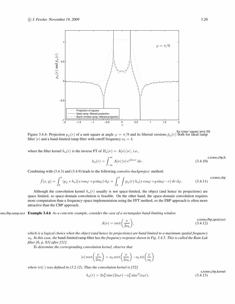
cf. [50, eqn. (14)]. Fig. 3.4.4 shows an example of the projection pϕ(r) of a unit square and its filtered version pϕ(r).
The ramp filter causes singularities at each of the points of discontinuity in the projections. (Compare with Fig. 3.3.4.)
For the case sinϕ = 0, see Problem 3.23.
3.4.5 Filtered versus unfiltered backprojection
Recall that an unfiltered backprojection of a sinogram gives an image blurred by 1/ |r|. This blurring is due to the
fact that the (all nonnegative) projection values “pile up” in the laminogram, and there is no destructive interference.
In contrast, after filtering with the ramp filter, the projections have both positive and negative values, so destructive
interference can occur, which is desirable for the parts of the image that are supposed to be zero for example. Fig. 3.3.4
illustrates these concepts.
3.4.6 The convolve-backproject (CBP) methods,tomo,cbp
The ramp filter amplifies high frequency noise, so in practice one must apodize it by a 1D lowpass filter A(ν), in which
case (3.4.2) is replaced by
pϕ(r) =
∫ ∞
−∞Pϕ(ν)A(ν) |ν| eı2πνr dν . (3.4.8)
e,tomo,fbp,A(u)
Alternatively, one can perform this filtering operation in the spatial domain by radial convolution:
pϕ(r) = pϕ(r) ∗ ha(r) =
∫
pϕ(r′)ha(r − r′) dr′, (3.4.9)e,tomo,cbp,conv
Page 20
c© J. Fessler. November 19, 2009 3.20
−2 −1.5 −1 −0.5 0 0.5 1 1.5 2−1
−0.5
0
0.5
1
Projection of square
Ideal ramp−filtered projection
Band−limited ramp−filtered projection
r
pϕ(r
)an
dp
ϕ(r
)
ϕ = π/9
Figure 3.4.4: Projection pϕ(r) of a unit square at angle ϕ = π/9 and its filtered versions pϕ(r) both for ideal ramp
filter |ν| and a band-limited ramp filter with cutoff frequency ν0 = 4.
fig˙tomo˙square˙proj˙filt
where the filter kernel ha(r) is the inverse FT of Ha(ν) = A(ν) |ν| , i.e.,
ha(r) =
∫ ∞
−∞A(ν) |ν| eı2πνr dν . (3.4.10)
e,tomo,cbp,h
Combining with (3.4.3) and (3.4.9) leads to the following convolve-backproject method:
f(x, y) =
∫ π
0
(pϕ ∗ ha)(x cosϕ+y sinϕ) dϕ =
∫ π
0
∫
pϕ(r) ha(x cosϕ +y sinϕ−r) dr dϕ . (3.4.11)e,tomo,cbp
Although the convolution kernel ha(r) usually is not space-limited, the object (and hence its projections) are
space limited, so space-domain convolution is feasible. On the other hand, the space-domain convolution requires
more computation than a frequency-space implementation using the FFT method, so the FBP approach is often more
attractive than the CBP approach.
x,tomo,fbp,ramp,rect Example 3.4.6 As a concrete example, consider the case of a rectangular band-limiting window
A(ν) = rect
(ν
2ν0
)
, (3.4.12)e,tomo,fbp,apod,rect
which is a logical choice when the object (and hence its projections) are band limited to a maximum spatial frequency
u0. In this case, the band-limited ramp filter has the frequency response shown in Fig. 3.4.5. This is called the Ram-Lak
filter [6, p. 83] after [51].
To determine the corresponding convolution kernel, observe that
|ν| rect(
ν
2ν0
)
= ν0 rect
(ν
2ν0
)
−ν0 tri
(ν
ν0
)
where tri(·) was defined in (3.2.12). Thus the convolution kernel is [52]
ha(r) = 2ν20 sinc(2ν0r)−ν2
0 sinc2(ν0r), (3.4.13)e,tomo,cbp,kernel
Page 21
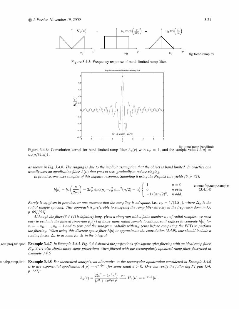
c© J. Fessler. November 19, 2009 3.21
= −Ha(ν) ν0 rect(
ν2ν0
)
ν0 tri(
νν0
)
νννν0 ν0 ν0
Figure 3.4.5: Frequency response of band-limited ramp filter.
fig˙tomo˙ramp˙tri
−8 −6 −4 −2 0 2 4 6 8−0.8
−0.6
−0.4
−0.2
0
0.2
0.4
0.6
0.8
1
Impulse response of bandlimited ramp filter
h(r) = 2 sinc(2r) − sinc2(r)
r
ha(r
)
Figure 3.4.6: Convolution kernel for band-limited ramp filter ha(r) with ν0 = 1, and the sample values h[n] =ha(n/(2ν0)) .
fig˙tomo˙ramp˙bandlimit
as shown in Fig. 3.4.6. The ringing is due to the implicit assumption that the object is band limited. In practice one
usually uses an apodization filter A(ν) that goes to zero gradually to reduce ringing.
In practice, one uses samples of this impulse response. Sampling it using the Nyquist rate yields [5, p. 72]:
h[n] = ha
(n
2ν0
)
= 2ν20 sinc(n)−ν2
0 sinc2(n/2) = ν20
1, n = 00, n even
−1/(πn/2)2, n odd.(3.4.14)
e,tomo,fbp,ramp,samples
Rarely is ν0 given in practice, so one assumes that the sampling is adequate, i.e., ν0 = 1/(2∆R), where ∆R is the
radial sample spacing. This approach is preferable to sampling the ramp filter directly in the frequency domain [5,
p. 69] [53].
Although the filter (3.4.14) is infinitely long, given a sinogram with a finite number nR of radial samples, we need
only to evaluate the filtered sinogram pϕ(r) at those same radial sample locations, so it suffices to compute h[n] for
n = −nR, . . . , nR − 1 and to zero pad the sinogram radially with nR zeros before computing the FFTs to perform
the filtering. When using this discrete-space filter h[n] to approximate the convolution (3.4.9), one should include a
scaling factor ∆R to account for dr in the integral.
x,tomo,fbp,rect,proj,filt,apod Example 3.4.7 In Example 3.4.5, Fig. 3.4.4 showed the projections of a square after filtering with an ideal ramp filter.
Fig. 3.4.4 also shows those same projections when filtered with the rectangularly apodized ramp filter described in
Example 3.4.6.
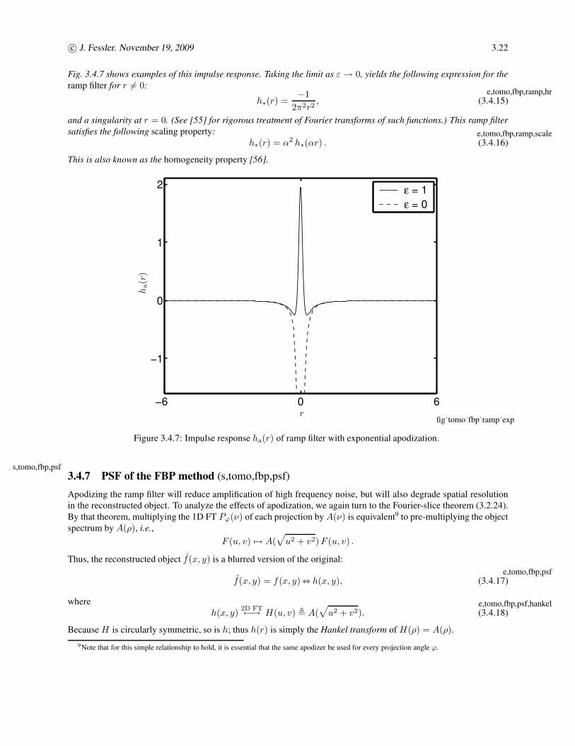
x,tomo,fbp,ramp,limit Example 3.4.8 For theoretical analysis, an alternative to the rectangular apodization considered in Example 3.4.6
is to use exponential apodization A(ν) = e−ε|ν| , for some small ε > 0. One can verify the following FT pair [54,
p. 127]:
ha(r) =2(ε2 − 4π2r2)
(ε2 + 4π2r2)2FT←→ Ha(ν) = e−ε|ν| |ν| .
Page 22
c© J. Fessler. November 19, 2009 3.22
Fig. 3.4.7 shows examples of this impulse response. Taking the limit as ε→ 0, yields the following expression for the
ramp filter for r 6= 0:
h∗(r) =−1
2π2r2, (3.4.15)
e,tomo,fbp,ramp,hr
and a singularity at r = 0. (See [55] for rigorous treatment of Fourier transforms of such functions.) This ramp filter
satisfies the following scaling property:
h∗(r) = α2 h∗(αr) . (3.4.16)e,tomo,fbp,ramp,scale
This is also known as the homogeneity property [56].
−6 0 6
−1
0
1
2ε = 1
ε = 0
r
ha(r
)
Figure 3.4.7: Impulse response ha(r) of ramp filter with exponential apodization.
fig˙tomo˙fbp˙ramp˙exp
3.4.7 PSF of the FBP method (s,tomo,fbp,psf)s,tomo,fbp,psf
Apodizing the ramp filter will reduce amplification of high frequency noise, but will also degrade spatial resolution
in the reconstructed object. To analyze the effects of apodization, we again turn to the Fourier-slice theorem (3.2.24).
By that theorem, multiplying the 1D FT Pϕ(ν) of each projection by A(ν) is equivalent9 to pre-multiplying the object
spectrum by A(ρ), i.e.,
F (u, v) 7→ A(√
u2 + v2)F (u, v) .
Thus, the reconstructed object f(x, y) is a blurred version of the original:
f(x, y) = f(x, y) ∗∗ h(x, y), (3.4.17)e,tomo,fbp,psf
where
h(x, y)2D FT←→ H(u, v) , A(
√
u2 + v2). (3.4.18)e,tomo,fbp,psf,hankel
Because H is circularly symmetric, so is h; thus h(r) is simply the Hankel transform of H(ρ) = A(ρ).
9Note that for this simple relationship to hold, it is essential that the same apodizer be used for every projection angle ϕ.
Page 23
c© J. Fessler. November 19, 2009 3.23
x,tomo,psf,rect Example 3.4.9 For the rectangular apodizing window A(ν) = rect(
ν2ν0
)
, the corresponding PSF in the image
domain would be
h(r) = ν20 jinc(ν0r) .
Thus the image would be blurred by a jinc function, which has large sidelobes that would cause undesirable “ringing.”
x,tomo,psf,gauss Example 3.4.10 A popular choice in nuclear medicine is a gaussian window: A(ν) = exp(−π(ν/ν0)
2). The half-
amplitude cutoff frequency ν1/2 for this window, i.e., the point where A(ν1/2) = A(0)/2, is ν1/2 = ν0
√log 2
π ≈ν0
2 0.9394 ≈ ν0
2 . Because the Hankel transform of a gaussian is gaussian, in the image domain the PSF is
h(r) = ν20 exp
(−π(ν0r)
2).
To find the FWHM of this gaussian, find r such that h(r) = h(0)/2, or exp(−π(ν0r)
2)
= 1/2 so π(ν0r)2 = log 2.
Thus
FWHM =2
ν0
√
log 2
π≈ 0.9394
ν0≈ 1
ν0≈ 1
2ν1/2.
So for a 5mm FWHM PSF, we would use ν0 = 1/5 = 0.2 cycles/cm.
x,tomo,fbp,other Example 3.4.11 Other popular window functions include the following.
• Hann or Hanning: A(ν) = [12 + 12 cos(πν/ν0)] rect
(ν
2ν0
)
• Hamming: A(ν) = [0.54 + 0.46 cos(πν/ν0)] rect(
ν2ν0
)
• Generalized Hamming: A(ν) = [α + (1− α) cos(πν/ν0)] rect(
ν2ν0
)
, for α ∈ [0, 1]
• Butterworth: A(ν) =1
√
1 + (ν/ν0)2n, for n ≥ 0
• Parzen: A(ν) =
1− 6(ν/ν0)2 (1− |ν| /ν0) |ν| ≤ ν0/2
2 (1− |ν| /ν0)3
ν0/2 ≤ |ν| ≤ ν0
0, otherwise
• Shepp Logan [57]: A(ν) =∣∣∣sinc
(ν
2ν0
)∣∣∣ or
∣∣∣sinc
(ν
2ν0
)∣∣∣
3
• Modified Shepp Logan: A(ν) = sinc(
ν2ν0
)
[0.4− 0.6 cos(πν/ν0)]
It is not always easy to find a closed-form expression for the PSF h that results from apodization. But the general
rule of thumb, FWHM ≈ 1/(2ν1/2), is usually pretty close.
In light of the result (3.4.17), one might wonder why we apply the window A(ν) to the projections rather than just
smooth (post-filter) the reconstructed image? The main reason is that we have to apply the ramp filter anyway, so we
can include A(ν) essentially for free. In contrast, post-smoothing would require either an “expensive” convolution
or a pair of 2D FFTs. However, if one wants to experiment with several different amounts of smoothing, then it is
preferable to smooth after a (ramp-filtered) backprojection so that only one backprojection operation is needed.
Summary
We have described three methods for inverting the Radon transform, i.e., for reconstructing a 2D object f(x, y) from
its projections {pϕ(r)}:• direct Fourier reconstruction (gridding),
• the backproject-filter (BPF) method (cone filter),
• the filter-backproject (FBP) method (ramp filter), and its cousin the convolve-backproject (CBP) method.
The derivations of these methods all used the Fourier-slice theorem. These methods would yield identical results for
noiseless continuous-space data, but are based on different manipulations of the formulas so they lead to different
ways of discretizing and implementing the equations, yielding very different numerical algorithms in practice.
We also analyzed the PSF due to windowing the ramp filter. In practice one must choose the apodizing window to
make a suitable compromise between spatial resolution and noise.
Page 24
c© J. Fessler. November 19, 2009 3.24
Recently, other inversion formulas for the 2D Radon transform have been discovered for objects with compact
support, e.g., [58]. These methods include user-selectable parameters that allow one to avoid corrupted or missing
regions of the sinogram. An interesting open problem is to determine whether the methods could be extended to
include some type of statistical weighting.
3.5 Practical backprojection (s,tomo,prac)s,tomo,prac
In the preceding sections, we have considered the idealized case where there is a continuum of projection views. In
practice, sinograms have only a finite number of angular samples, so each of the reconstruction methods described in
§3.4 requires modification for practical implementations.
A critical step in both the BPF and FBP reconstruction methods is the backprojection operation (3.3.1). Given only
a finite number nϕ of projection angles, we must approximate the integral in (3.3.1). Usually the projection angles are
uniformly spaced over the interval [0, π), i.e.,
ϕi =
(i− 1
nϕ
)
π, i = 1, . . . , nϕ.
In such cases, the usual approach is to use the following Riemann sum approximation to (3.3.1):
fb(x, y) ≈ π
nϕ
nϕ∑
i=1
pϕi(x cosϕi +y sinϕi). (3.5.1)
e,tomo,prac,back
Whether more sophisticated approximations to this integral would be beneficial is an open problem.
There are at least three distinct approaches to implementing (3.5.1): rotation-based backprojection, ray-driven
backprojection, and pixel-driven backprojection. If the available projections were continuous functions of the radial
argument, then these formulations would be identical. In practice, not only are the projection angles discrete, but
also we only have discrete radial samples of pϕ(r), as described in (4.3.1). Ignoring noise and blur, we are given the
discrete sinogram
yi[n] = pϕ(r)∣∣∣ϕ=ϕi, r=rc[n]
, i = 1, . . . , nϕ, n = 0, . . . , nR − 1, (3.5.2)e,tomo,prac,sample
where the radial sample locations are given by
rc[n] = (n− n0)∆R (3.5.3)e,tomo,prac,rcn
and typically n0 = nR/2 or n0 = (nR − 1)/2. For such sinograms, the various backprojection methods can produce
different results because they differ in how the equations are discretized.
If the true object f true can be assumed to be appropriately band limited, then its projections will also be band
limited (by the Fourier slice theorem), so in principle we could recover pϕifrom {yi[·]} using sinc interpolation:
pϕi(r) =
∞∑
n=−∞yi[n] sinc
(r − rc[n]
∆R
)
.
In practice this interpolation is inappropriate because: real objects are space limited so they cannot be band limited, sinc
interpolation expects an infinite number of samples whereas practical sinograms have only a finite number of samples,
and sinc interpolation is computationally impractical. Thus, simpler interpolation methods are used in practice, such
as linear interpolation or spline interpolation [59], perhaps combined with oversampling of the FFT used for the ramp
filter.
3.5.1 Rotation-based backprojection
We can rewrite the backprojection formula (3.5.1) as follows:
fb(x, y) =π
nϕ
nϕ∑
i=1
bi(x, y), (3.5.4)e,tomo,prac,back,ray
Page 25
c© J. Fessler. November 19, 2009 3.25
where the backprojection of the ith view is given by:
bi(x, y) = pϕi(x cosϕi +y sinϕi).
We can also write bi = P∗ϕi
pϕi, where P
∗ϕi
is defined in (4.2.4). This adjoint maps the ith 1D projection back
into a 2D object by “smearing” that projection along the angle ϕi. In this approach, we form temporary images by
backprojecting each view and accumulating the sum of those temporary images.
To better understand bi(x, y), note that when i = 1 we have ϕ = 0, so
b1(x, y) = p0(x),
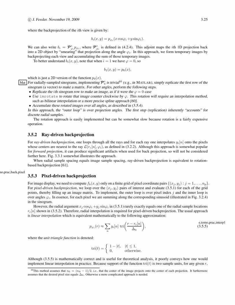
which is just a 2D version of the function p0(x).Mat For radially-sampled sinograms, implementing P
∗0 is trivial10 (e.g., in MATLAB), simply replicate the first row of the
sinogram (a vector) to make a matrix. For other angles, perform the following steps.
• Replicate the ith sinogram row to make an image, as if it were the ϕ = 0 case
• Use imrotate to rotate that image counter clockwise by ϕ. This rotation will require an interpolation method,
such as bilinear interpolation or a more precise spline approach [60].
• Accumulate these rotated images over all angles, as described in (3.5.4).
In this approach, the “outer loop” is over projection angles. The first step (replication) inherently “accounts” for
discrete radial samples.
The rotation approach is easily implemented but can be somewhat slow because rotation is a fairly expensive
operation.
3.5.2 Ray-driven backprojection
For ray-driven backprojection, one loops through all the rays and for each ray one interpolates yi[n] onto the pixels
whose centers are nearest to the ray L(rc[n], ϕi), as defined in (3.2.2). Although this approach is somewhat popular
for forward projection, it can produce significant artifacts when used for back projection, so will not be considered
further here. Fig. 3.3.1 somewhat illustrates the approach.
When radial sample spacing equals image sample spacing, ray-driven backprojection is equivalent to rotation-
based backprojection [61].
3.5.3 Pixel-driven backprojections,tomo,prac,back,pixel
For image display, we need to compute fb(x, y) only on a finite grid of pixel coordinate pairs {(xj , yj) : j = 1, . . . , np}.For pixel-driven backprojection, we loop over the (xj , yj) pairs of interest and evaluate (3.5.1) for each of the grid
points, thereby filling up an image matrix. To implement, the outer loop is over pixel index j and the inner loop is
over angles ϕi. In essence, for each pixel we are summing along the corresponding sinusoid (illustrated in Fig. 3.2.4)
in the sinogram.
However, the radial argument xj cosϕi +yj sinϕi in (3.5.1) rarely exactly equals one of the radial sample locations
rc[n] shown in (3.5.2). Therefore, radial interpolation is required for pixel-driven backprojection. The usual approach
is linear interpolation which is equivalent mathematically to the following approximation:
pϕi(r) ≈
∑
n
yi[n] tri
(r − rc[n]
∆R
)
, (3.5.5)e,tomo,prac,interp1
where the unit triangle function is denoted:
tri(t) =
{1− |t|, |t| ≤ 1,0, otherwise.
Although (3.5.5) is mathematically correct and is useful for theoretical analysis, it poorly conveys how one would
implement linear interpolation in practice. Because support of the function tri(t) is two sample units, for any given r,
10This method assumes that n0 = (nR − 1)/2, i.e., that the center of the image projects onto the center of each projection. It furthermore
assumes that the desired pixel size equals ∆R. Otherwise a more complicated approach is needed.
Page 26
c© J. Fessler. November 19, 2009 3.26
only two terms in the sum in (3.5.5) are possibly nonzero. An alternative expression is
pϕi(r) ≈ yi[n(r)] tri
(r − rc[n(r)]
∆R
)
+yi[n(r) + 1] tri
(r − rc[n(r) + 1]
∆R
)
= yi[n(r)]
(
1− r − rc[n(r)]
∆R
)
+ yi[n(r) + 1]
(r − rc[n(r)]
∆R
)
,
where we define
n(r) , ⌊r/∆R + n0⌋ .Other interpolators, such as an oversampled FFT or spline functions are also used [59].
3.5.4 Interpolation effectss,tomo,prac,interp
Generalizing (3.5.5), suppose that we use an interpolation method of the form:
pϕi(r) =
∑
n
yi[n] h
(r − rc[n]
∆R
)
for some interpolation kernel h(·). Suppose furthermore that pϕ(r) is band limited with maximum frequency less than1
2∆R. Then it follows from (3.5.2) and the sampling theorem that (ignoring noise):
Pϕi(ν) =
{Pϕi
(ν) H(ν), |ν| < 12∆R
0, otherwise.
For example, when h is the linear interpolator in (3.5.5), we have H(ν) = ∆R sinc2(∆Rν), which is strictly positive
for |ν| < 12∆R
. Therefore, while we are applying the ramp filter |ν| in the discretized version of (3.4.2), we can also
apply the inverse filter 1/H(ν) to compensate for the effects of interpolation [62, eqn. (45)] [59, 63].
Summary
Pixel-driven, rotation-based, and ray-driven backprojection are all used in practice, depending on number of samples,
sample spacing, etc. The formulations are exactly identical in continuous space, but can yield slightly different results
when discretized.
3.6 Sinogram restoration (s,tomo,restore)s,tomo,restore
Because a sinogram pϕ(r) has two coordinates (r and ϕ), one can display it as a 2D picture or even treat it as a 2D
“image” and apply any number of image processing methods to it. Numerous linear and nonlinear filters have been
applied to sinograms in an attempt to reduce noise [64–84] to extrapolate missing data [85–88] and to compensate
for detector blur [89–96] and/or SPECT attenuation [97–100]. Some of these methods can even be called “statistical”
methods because they include measurement noise models. Problem 3.12 explores an approach based on B-splines.
A typical linear approach for a system with shift-invariant blur having frequency response B(ν) would be to use a
Wiener filter as the apodizing filter A(ν) in (3.4.8) as follows
A(ν) =B∗(ν)
|B(ν)|2 + Sp(ν),
where Sp(ν) is some model for the power spectral density of pϕ(r) under the (questionable) assumption that pϕ(r) is
a WSS random process.
Nonlinear sinogram preprocessing methods, including classical methods based on view-adaptive Wiener filters
[101] and contemporary approaches like wavelet-based denoising [102], have the potential to reduce noise more than
linear methods with less degradation of spatial resolution. However, when a nonlinear sinogram filtering method is
combined with the linear FBP reconstruction method the resulting spatial resolution properties can be quite unusual.
It is the author’s view that nonlinear processing is more safely performed in the image domain, e.g., by nonquadratic
edge-preserving regularization, instead of in the sinogram domain.
Page 27
c© J. Fessler. November 19, 2009 3.27
3.7 Sampling considerations (s,tomo,samp)s,tomo,samp
In practice one can only acquire a finite number of radial and angular samples, due to constraints such as cost and
time. This section describes considerations in choosing the radial and angular sampling.
3.7.1 Radial sampling
The radial sample spacing, ∆R, should be determined by the spatial resolution (in the radial direction) of the tomo-
graphic scanning instrument. The FWHM of the system radial resolution is a function of the detector width, the
source size in X-ray imaging, etc. The radial detector response (e.g., a rectangular function for square detector el-
ements) generally is not exactly band-limited, so Nyquist sampling theory can provide only general guidance. A
practical rule-of-thumb is to choose (if possible): ∆R = FWHM/2. Then the number of radial samples should be
determined to cover the desired FOV by choosing: nR = FOV/∆R. See §4.3.9 for Fourier analysis of aliasing due to
radial sampling.
3.7.2 Angular samplings,tomo,samp,ang
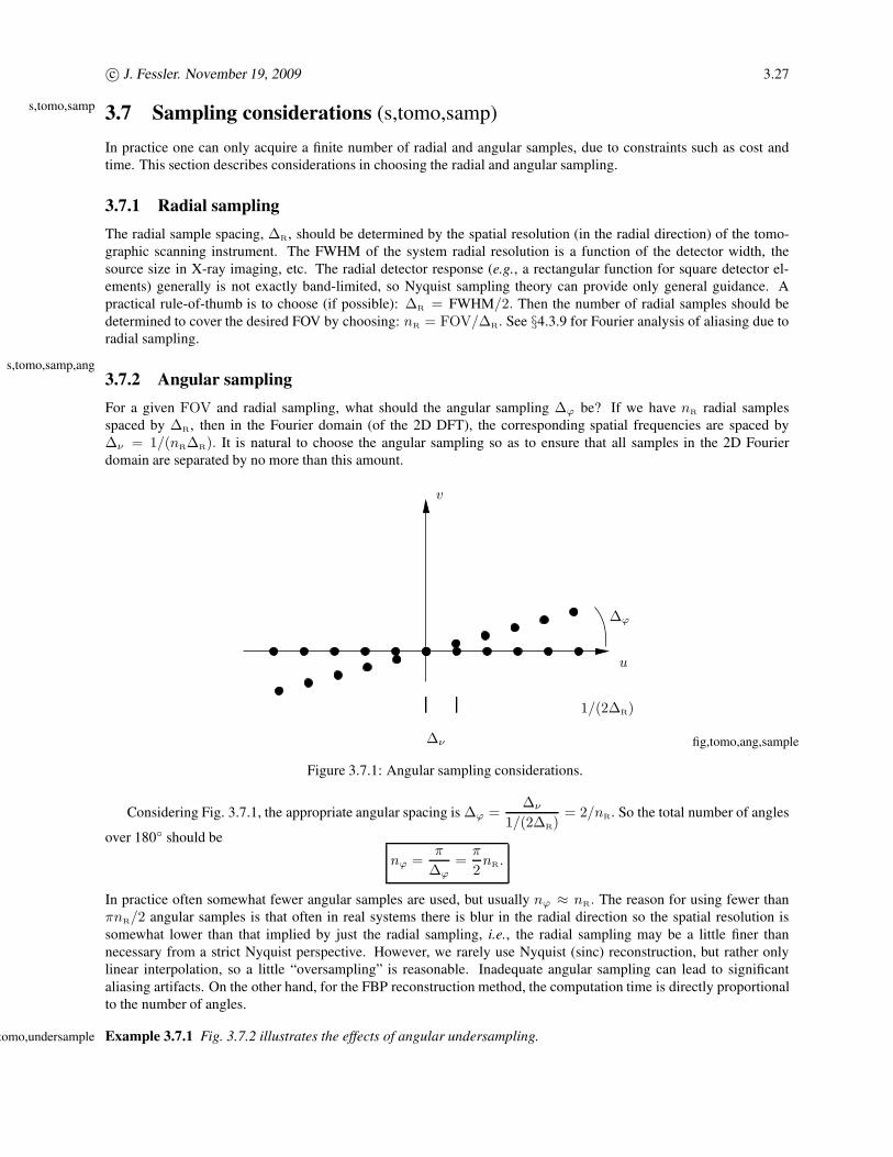
For a given FOV and radial sampling, what should the angular sampling ∆ϕ be? If we have nR radial samples
spaced by ∆R, then in the Fourier domain (of the 2D DFT), the corresponding spatial frequencies are spaced by
∆ν = 1/(nR∆R). It is natural to choose the angular sampling so as to ensure that all samples in the 2D Fourier
domain are separated by no more than this amount.
u
v
∆ν
∆ϕ
1/(2∆R)
Figure 3.7.1: Angular sampling considerations.
fig,tomo,ang,sample
Considering Fig. 3.7.1, the appropriate angular spacing is ∆ϕ =∆ν
1/(2∆R)= 2/nR. So the total number of angles
over 180◦ should be
nϕ =π
∆ϕ=
π
2nR.
In practice often somewhat fewer angular samples are used, but usually nϕ ≈ nR. The reason for using fewer than
πnR/2 angular samples is that often in real systems there is blur in the radial direction so the spatial resolution is
somewhat lower than that implied by just the radial sampling, i.e., the radial sampling may be a little finer than
necessary from a strict Nyquist perspective. However, we rarely use Nyquist (sinc) reconstruction, but rather only
linear interpolation, so a little “oversampling” is reasonable. Inadequate angular sampling can lead to significant
aliasing artifacts. On the other hand, for the FBP reconstruction method, the computation time is directly proportional
to the number of angles.
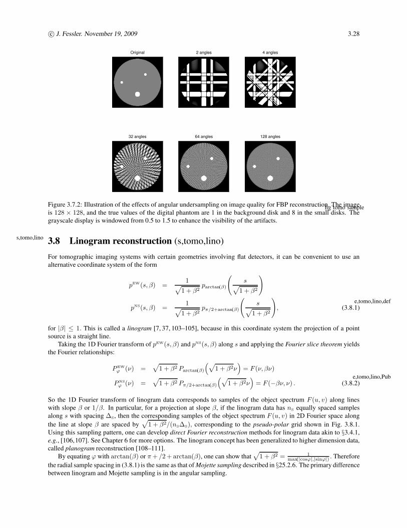
x,tomo,undersample Example 3.7.1 Fig. 3.7.2 illustrates the effects of angular undersampling.
Page 28
c© J. Fessler. November 19, 2009 3.28
Original 2 angles 4 angles
32 angles 64 angles 128 angles
Figure 3.7.2: Illustration of the effects of angular undersampling on image quality for FBP reconstruction. The image
is 128 × 128, and the true values of the digital phantom are 1 in the background disk and 8 in the small disks. The
grayscale display is windowed from 0.5 to 1.5 to enhance the visibility of the artifacts.
fig˙tomo˙sample
3.8 Linogram reconstruction (s,tomo,lino)s,tomo,lino
For tomographic imaging systems with certain geometries involving flat detectors, it can be convenient to use an
alternative coordinate system of the form
pEW(s, β) =1
√
1 + β2parctan(β)
(
s√
1 + β2
)
pNS(s, β) =1
√
1 + β2pπ/2+arctan(β)
(
s√
1 + β2
)
, (3.8.1)e,tomo,lino,def
for |β| ≤ 1. This is called a linogram [7, 37, 103–105], because in this coordinate system the projection of a point
source is a straight line.
Taking the 1D Fourier transform of pEW(s, β) and pNS(s, β) along s and applying the Fourier slice theorem yields
the Fourier relationships:
P EW
ϕ (ν) =√
1 + β2 Parctan(β)
(√
1 + β2ν)
= F (ν, βν)
PNS
ϕ (ν) =√
1 + β2 Pπ/2+arctan(β)
(√
1 + β2ν)
= F (−βν, ν) . (3.8.2)e,tomo,lino,Pub
So the 1D Fourier transform of linogram data corresponds to samples of the object spectrum F (u, v) along lines
with slope β or 1/β. In particular, for a projection at slope β, if the linogram data has nS equally spaced samples
along s with spacing ∆S, then the corresponding samples of the object spectrum F (u, v) in 2D Fourier space along
the line at slope β are spaced by√
1 + β2/(nS∆S), corresponding to the pseudo-polar grid shown in Fig. 3.8.1.
Using this sampling pattern, one can develop direct Fourier reconstruction methods for linogram data akin to §3.4.1,
e.g., [106,107]. See Chapter 6 for more options. The linogram concept has been generalized to higher dimension data,
called planogram reconstruction [108–111].
By equating ϕ with arctan(β) or π + /2 + arctan(β), one can show that√
1 + β2 = 1max(|cosϕ|,|sinϕ|) . Therefore
the radial sample spacing in (3.8.1) is the same as that of Mojette sampling described in §25.2.6. The primary difference
between linogram and Mojette sampling is in the angular sampling.
Page 29
c© J. Fessler. November 19, 2009 3.29
u
v
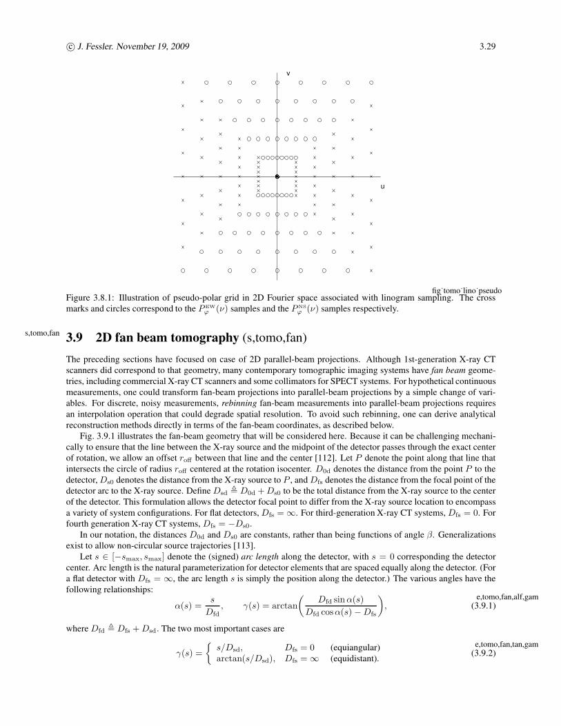
Figure 3.8.1: Illustration of pseudo-polar grid in 2D Fourier space associated with linogram sampling. The cross
marks and circles correspond to the P EW
ϕ (ν) samples and the PNS
ϕ (ν) samples respectively.
fig˙tomo˙lino˙pseudo
3.9 2D fan beam tomography (s,tomo,fan)s,tomo,fan
The preceding sections have focused on case of 2D parallel-beam projections. Although 1st-generation X-ray CT
scanners did correspond to that geometry, many contemporary tomographic imaging systems have fan beam geome-
tries, including commercial X-ray CT scanners and some collimators for SPECT systems. For hypothetical continuous
measurements, one could transform fan-beam projections into parallel-beam projections by a simple change of vari-
ables. For discrete, noisy measurements, rebinning fan-beam measurements into parallel-beam projections requires
an interpolation operation that could degrade spatial resolution. To avoid such rebinning, one can derive analytical
reconstruction methods directly in terms of the fan-beam coordinates, as described below.
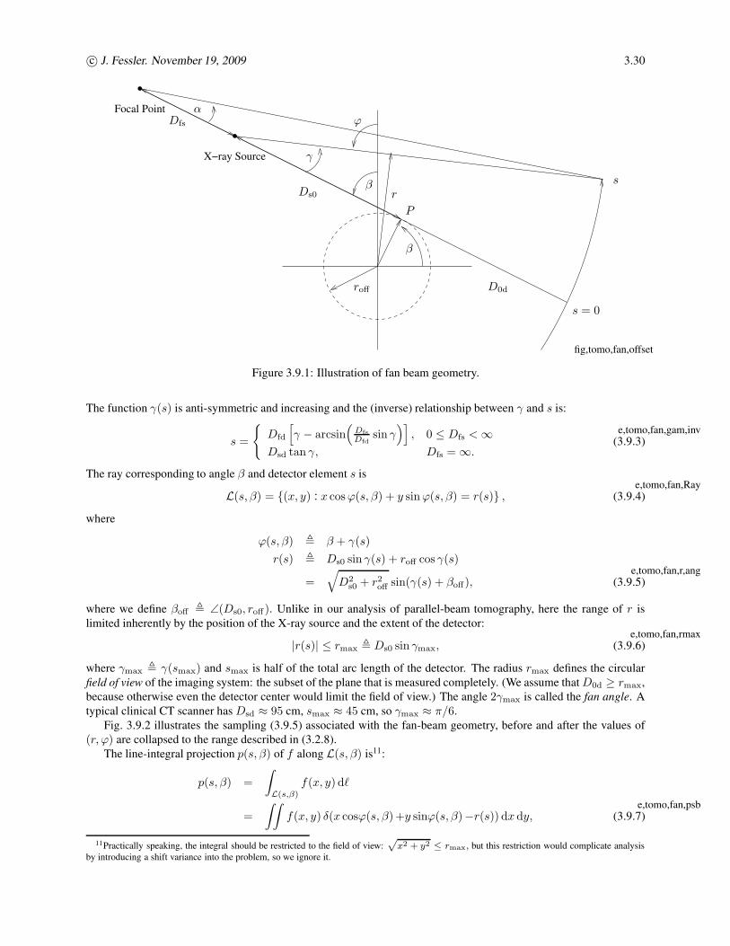
Fig. 3.9.1 illustrates the fan-beam geometry that will be considered here. Because it can be challenging mechani-
cally to ensure that the line between the X-ray source and the midpoint of the detector passes through the exact center
of rotation, we allow an offset roff between that line and the center [112]. Let P denote the point along that line that
intersects the circle of radius roff centered at the rotation isocenter. D0d denotes the distance from the point P to the
detector, Ds0 denotes the distance from the X-ray source to P , and Dfs denotes the distance from the focal point of the
detector arc to the X-ray source. Define Dsd , D0d + Ds0 to be the total distance from the X-ray source to the center
of the detector. This formulation allows the detector focal point to differ from the X-ray source location to encompass
a variety of system configurations. For flat detectors, Dfs =∞. For third-generation X-ray CT systems, Dfs = 0. For
fourth generation X-ray CT systems, Dfs = −Ds0.
In our notation, the distances D0d and Ds0 are constants, rather than being functions of angle β. Generalizations
exist to allow non-circular source trajectories [113].
Let s ∈ [−smax, smax] denote the (signed) arc length along the detector, with s = 0 corresponding the detector
center. Arc length is the natural parameterization for detector elements that are spaced equally along the detector. (For
a flat detector with Dfs = ∞, the arc length s is simply the position along the detector.) The various angles have the
following relationships:
α(s) =s
Dfd, γ(s) = arctan
(Dfd sin α(s)
Dfd cosα(s) −Dfs
)
, (3.9.1)e,tomo,fan,alf,gam
where Dfd , Dfs + Dsd. The two most important cases are
γ(s) =
{s/Dsd, Dfs = 0 (equiangular)
arctan(s/Dsd), Dfs =∞ (equidistant).(3.9.2)e,tomo,fan,tan,gam
Page 30
c© J. Fessler. November 19, 2009 3.30
X−ray Source
Focal Pointϕ
α
β
β
γ
rs
s = 0
roff
P
Dfs
Ds0
D0d
Figure 3.9.1: Illustration of fan beam geometry.
fig,tomo,fan,offset
The function γ(s) is anti-symmetric and increasing and the (inverse) relationship between γ and s is:
s =
{
Dfd
[
γ − arcsin(
Dfs
Dfdsin γ
)]
, 0 ≤ Dfs <∞Dsd tan γ, Dfs =∞.
(3.9.3)e,tomo,fan,gam,inv
The ray corresponding to angle β and detector element s is
L(s, β) = {(x, y) : x cos ϕ(s, β) + y sin ϕ(s, β) = r(s)} , (3.9.4)e,tomo,fan,Ray
where
ϕ(s, β) , β + γ(s)
r(s) , Ds0 sinγ(s) + roff cos γ(s)
=√
D2s0 + r2
off sin(γ(s) + βoff), (3.9.5)e,tomo,fan,r,ang
where we define βoff , ∠(Ds0, roff). Unlike in our analysis of parallel-beam tomography, here the range of r is
limited inherently by the position of the X-ray source and the extent of the detector:
|r(s)| ≤ rmax , Ds0 sin γmax, (3.9.6)e,tomo,fan,rmax
where γmax , γ(smax) and smax is half of the total arc length of the detector. The radius rmax defines the circular
field of view of the imaging system: the subset of the plane that is measured completely. (We assume that D0d ≥ rmax,
because otherwise even the detector center would limit the field of view.) The angle 2γmax is called the fan angle. A
typical clinical CT scanner has Dsd ≈ 95 cm, smax ≈ 45 cm, so γmax ≈ π/6.
Fig. 3.9.2 illustrates the sampling (3.9.5) associated with the fan-beam geometry, before and after the values of
(r, ϕ) are collapsed to the range described in (3.2.8).
The line-integral projection p(s, β) of f along L(s, β) is11:
p(s, β) =
∫
L(s,β)
f(x, y) dℓ
=
∫∫
f(x, y) δ(x cosϕ(s, β)+y sinϕ(s, β)−r(s)) dx dy, (3.9.7)e,tomo,fan,psb
11Practically speaking, the integral should be restricted to the field of view:p
x2 + y2 ≤ rmax, but this restriction would complicate analysis
by introducing a shift variance into the problem, so we ignore it.
Page 31
c© J. Fessler. November 19, 2009 3.31
−0.5 0 0.5
0
π
−0.5 0 0.5
0
π
−0.5 0 0.5
0
π
−0.5 0 0.5
0
π
r/Ds0r/Ds0
r/Ds0r/Ds0
ϕϕ
ϕϕ
β = 0
β = 0
β = 3π/2
β = 3π/2
Figure 3.9.2: Left: (r, ϕ) coordinates for equiangular fan-beam samples based directly on (3.9.5). The fan angle is
2γmax = π/3. Right: after converting ϕ to the range [0, π) using the periodicity property (3.2.19). Top: for equally
spaced samples in s symmetrical around s = 0. Bottom: for equally spaced samples in s with quarter-detector offset.
The samples for one particular value of β are circled for illustration.
fig˙tomo˙fan˙sample
for |s| ≤ smax and 0 ≤ β < βmax. We assume βmax ≥ π +2γmax to ensure complete sampling. By (3.9.5), fan-beam
projections satisfy the following general symmetry property:
p(γ−1(−γ(s)− 2βoff) , β ± π + 2γ(s) + 2βoff
)= p(s, β) . (3.9.8)
e,tomo,fan,sym
In particular, if Dfs = 0, then
p(−s− 2Dsdβoff , β ± π + 2s/Dsd + 2βoff) = p(s, β) . (3.9.9)e,tomo,fan,sym,Dfs=0
Alternatively, if βoff = 0, then
p(−s, β ± π + 2γ(s)) = p(s, β) . (3.9.10)e,tomo,fan,sym,boff=0
The reconstruction problem is to estimate f from the fan-beam projections {p(s, β)}.
3.9.1 Fan-parallel rebinning methods (s,tomo,fan,rebin)s,tomo,fan,rebin
In continuous space, to rebin from fan-beam to parallel-beam coordinates requires a simple change of variables based
on (3.9.5). In the usual case where roff = 0, we can express the parallel-beam projections in terms of the fan-beam
projections using the following relationship:
pϕ(r) = p(s, β)∣∣∣s=s(r), β=β(r,φ)
= p(γ−1(arcsin(r/Ds0)) , φ− arcsin(r/Ds0)
), (3.9.11)
e,tomo,fan,rebin
Page 32
c© J. Fessler. November 19, 2009 3.32
where γ−1 is defined by (3.9.3). For sampled measurements, usually one first performs 1D interpolation along the
source position using the relationship φ = β + γ. Then one performs 1D interpolation along the detector by relating rand s. When the s samples include a quarter detector offset, then the radial sampling can be improved by a factor of
two, at least for 360◦ scans, as illustrated in Fig. 3.9.2.
IRT See rebin_fan2par.m.
3.9.2 The filter-backproject (FBP) approach for 360◦ scans (s,tomo,fan,fbp)s,tomo,fan,fbp
This section derives filter-backproject methods for the fan-beam geometry shown in Fig. 3.9.1, including the case of
displaced center of rotation [112]. We focus on the case of 360◦ rotation of the X-ray source and detector [5, p. 77].
We start by rewriting the parallel-ray FBP formula (3.4.11) for the case of 360◦ rotation:
f(x, y) =1
2
∫ 2π
0
∫
pϕ(r) h∗(x cosϕ+y sinϕ−r) dr dϕ, (3.9.12)e,tomo,fan,fbp,360
where h∗(·) denotes the ramp filter in (3.4.15) with 1D Fourier transform H∗(ν) = |ν|.Now change to fan-beam coordinates by making the transformation of variables r = r(s), ϕ = ϕ(s, β), defined
in (3.9.5). The Jacobian matrix is
[∂∂sr(s) ∂
∂β r(s)∂∂sϕ(s, β) ∂
∂β ϕ(s, β)
]
=
[[Ds0 cos γ(s)− roff sin γ(s)] γ(s) 0
γ(s) 1
]
, (3.9.13)e,tomo,fan,J
the determinant of which is
J(s) , |Ds0 cos γ(s)− roff sin γ(s)| |γ(s)| . (3.9.14)e,tomo,fan,detJ
The reconstruction formula becomes
f(x, y) =1
2
∫ 2π
0
∫
p(s, β) h∗(x cosϕ(s, β) + y sin ϕ(s, β) − r(s)) J(s) ds dβ
=1
2
∫ 2π
0
∫
p(s, β) J(s)h∗(x cos(β + γ(s)) + y sin(β + γ(s))−Ds0 sin γ(s)− roff cos γ(s)) ds dβ .
Although this expression is a fan-beam reconstruction formula, it is inconvenient for practical use; the challenge is to
manipulate it so that it has a filter-backproject form.
Using trigonometric identities, one can simplify the argument of h∗ above as follows:
x cos(β + γ)+y sin(β + γ)−Ds0 sin γ − roff cos γ = L(x, y, β) sin(γ′(x, y, β)−γ), (3.9.15)e,tomo,fan,fbp,h,arg
where
xβ , x cos β + y sin β
yβ , −x sin β + y cosβ
L(x, y, β) ,
√
(Ds0 − yβ)2 + (xβ − roff)2
γ′(x, y, β) , tan−1
(xβ − roff
Ds0 − yβ
)
. (3.9.16)e,tomo,fan,L,gam
Defining s′ by γ′ = γ(s′), using (3.9.15), and applying the scaling property of the ideal ramp filter12 (3.4.16) leads to
the following form for the fan-beam reconstruction formula:
f(x, y) =1
2
∫ 2π
0
∫
p(s, β)J(s)h∗(L(x, y, β) sin(γ′(x, y, β)−γ(s))) ds dβ
=1
2
∫ 2π
0
∫
p(s, β)J(s)
(s′(x, y, β)−s
L(x, y, β) sin(γ′(x, y, β)−γ(s))
)2
h∗(s′(x, y, β)−s) ds dβ .
12Zeng et al. note that using this property leads to nonuniform image noise variance in practice [56] and propose an alternative approach based
on Hilbert transforms [114].
Page 33
c© J. Fessler. November 19, 2009 3.33
For certain special fan-beam geometries, we can express the sin term above as follows:
sin(γ′(x, y, β)−γ(s)) = W2(x, y, β)W1(s)W0(s′(x, y, β)−s), (3.9.17)
e,tomo,fan,fbp,sin
for some geometry-dependentweighting functions W0, W1, and W2. For such geometries, the fan-beam reconstruction
formula simplifies as follows:
f(x, y) =1
2
∫ 2π
0
1
W 22 (x, y, β) L2(x, y, β)
[∫
p(s, β)J(s)
W 21 (s)
g(s′(x, y, β)−s) ds
]
dβ,
where we define the following modified ramp filter:
g(s) ,
(s
W0(s)
)2
h∗(s) . (3.9.18)e,tomo,fan,ramp,gen
Thus, the fan-beam FBP method uses the following three steps.
• Step 1. Compute weighted projections:
p(s, β) , p(s, β)J(s)
W 21 (s)
. (3.9.19)e,tomo,fan,psb,weight
• Step 2. Filter those weighted projections using the modified ramp filter:
p(s, β) , p(s, β) ∗g(s), ∀β.
• Step 3. Perform a weighted backprojection of those filtered projections:
f(x, y) =1
2
∫ 2π
0
1
W 22 (x, y, β)L2(x, y, β)
p(s′(x, y, β), β) dβ . (3.9.20)e,tomo,fan,fbp,wtd,back
This three-step procedure is quite practical and has been used routinely in commercial X-ray CT systems.
The existence of this efficient FBP approach hinges on whether a factorization of the form (3.9.17) exists. Besson
has shown that there are exactly four fan-beam geometries for which this is possible [113]. Fortunately, two of the four
cases are the important ones described in (3.9.2). Somewhat unfortunately, the 4th generation CT scanner geometry is
not one of the four cases, although most commercial CT scanners are 3rd generation.
3.9.2.1 Equiangular case
The case where Dfs = 0 corresponds to 3rd-generation X-ray CT systems using an arc detector, called the equiangular
case [115]. In this case, γ(s) = s/Dsd, so we factor the sin term in (3.9.17) as follows:
sin(γ′(x, y, β)−γ(s)) = W2 W0(s′(x, y, β)−s),
where W2 =1
Dsd, W0(s) = Dsd sin
(s
Dsd
)
, s′(x, y, β) = Dsd γ′(x, y, β),
with W1 = 1. Thus the modified ramp filter (3.9.18) is
g(s) =
(s/Dsd
sin(s/Dsd)
)2
h∗(s) . (3.9.21)e,tomo,fan,ramp,ea
Because γ(s) = 1/Dsd, the projection weighting in (3.9.19) simplifies to
J(s)
W 21
= J(s) =1
Dsd
∣∣∣∣Ds0 cos
s
Dsd− roff sin
s
Dsd
∣∣∣∣≈ Ds0
Dsdcos
s
Dsd, (3.9.22)
e,tomo,fan,J˙w1w1,ea
and the backprojection weighting in (3.9.20) is
1
W 22 L2(x, y, β)
=D2
sd
L2(x, y, β)=
D2sd
(Ds0 − yβ)2 + (xβ − roff)2. (3.9.23)
e,tomo,fan,fbp,w2,ea
Page 34
c© J. Fessler. November 19, 2009 3.34
Note that as Ds0 → ∞, i.e., as the rays become more parallel, the modified ramp filter approaches the usual ramp
filter, and the projection and backprojection weightings approach unity, as expected for the parallel-ray case.
For practical implementation the filter must be band-limited and sampled. Combining (3.9.21) with (3.4.14) for
ha(r), the necessary filter samples are
h[n] =
1
4∆2s
, n = 0
0, n even−1
[πDsd sin(n∆s/Dsd)]2 , n odd,
(3.9.24)e,tomo,fan,ramp,ea,sample
where ∆s denotes the detector element spacing. (Note that there is an error in [5, eqn. (96)].)
There is a subtle issue in the above derivation [56, 114]. We first applied the scaling property of the ramp filter,
continued the derivation, and then eventually considered a band-limited ramp filter (3.9.24). If we had considered
the band-limiting effect first, which might be more appropriate for sampled data, then the scaling property would not
hold exactly. It has been stated that this practice “results in a nonstationary cutoff frequency in the image” [56, 114].
Nevertheless, it is used widely.
IRT See fbp_ramp.m.
IRT See fbp_fan_arc.m.
3.9.2.2 Equidistant cases,tomo,fan,ea
The case where Dfs = ∞ corresponds to a flat detector, called the equidistant case [116]. In this case, γ(s) =arctan(s/Dsd) and (with some trigonometric identities) we factor the sin term in (3.9.17) as follows:
sin(γ′ − γ) = sinγ′ cos γ − sin γ cos γ′ = cos γ′ cos γ (tan γ′ − tan γ) = cos γ′ Dsd√
D2sd + s2
s′ − s
Dsd,
where s′(x, y, β) = Dsd tan γ′(x, y, β), or equivalently:
W2 =cos γ′(x, y, β)
Dsd, W1 =
Dsd√
D2sd + s2
, W0(s) = s.
Because W0(s) = s, we can use the usual ramp filter (3.4.14) without modification. Because γ(s) = (cos2 γ(s))/Dsd =W 2
1 (s) /Dsd here, the projection weighting in (3.9.19) becomes
J(s)
W 21
=1
Dsd|Ds0 cos γ(s)− roff sin γ(s)| ≈ Ds0
√
D2sd + s2
, (3.9.25)e,tomo,fan,J˙w1w1,ed
and the backprojection weighting in (3.9.20) is
1
W 22 L2(x, y, β)
=D2
sd
[cos γ′(x, y, β)L(x, y, β)]2=
D2sd
[Ds0 − yβ ]2. (3.9.26)
e,tomo,fan,wtb,ed
Note that as Ds0 →∞, the projection and backprojection weightings again approach unity.
IRT See fbp_fan_flat.m.
The preceding derivation started with the parallel-ray FBP formula. Other formulations are possible, e.g., [117].
3.9.3 FBP for short scans (s,tomo,fan,short)s,tomo,fan,short
The preceding analyses have assumed a full 360◦ rotation. For a 360◦ rotation, every ray is sampled exactly twice,
leading to the 1/2 factor in (3.9.12). There are also fan-beam reconstruction methods that use a short scan with less
than a full rotation. A standard short scan uses βmax = π + 2γmax, so that every point in the equivalent parallel-
beam sinogram is sampled at least once. As illustrated in Fig. 3.9.3, some areas of the sinogram are sampled twice, so
these methods require appropriate weighting, sometimes called Parker weighting [118]. In particular, by the symmetry
property (3.9.10), fan-beam sinogram data where 0 < β < 2(γmax−γ(s)) correspond to the same rays as π−2γ(s) <β < π + 2γmax.
Page 35
c© J. Fessler. November 19, 2009 3.35
One can compensate for this sampling by applying an additional weighting w(s, β) to the ramp-filtered fan-beam
sinogram p(s, β) prior to backprojection, such as the following weighting:
w(s, β) =
q(
β2(γmax−γ)
)
, 0 ≤ β ≤ 2(γmax − γ)
1, 2(γmax − γ) < β < π − 2γ
q(
π+2γmax−β2(γmax+γ)
)
, π − 2γ ≤ β ≤ π + 2γmax,
(3.9.27)e,tomo,fan,short,wsb
where q(x) = sin2(
π2 x)
and γ = γ(s). Note that [118, eqn. (12)] has a typo.
IRT See fbp_fan_short_wt.m.
ππ − γmax
3γmax
γmax
γ
ϕ Parker weighting
−25 −20 −15 −10 −5 0 5 10 15 20 25
0
50
100
150
200
0
1
γ [degrees]
β[d
egre
es]
Figure 3.9.3: For short scan with βmax = π + 2γmax, the left figure above illustrates (by darker shading) the areas
of a sinogram (in φ, γ space) that are sampled twice. The other areas are sampled once. The right figure shows the
fan-beam sinogram Parker weighting (3.9.27).
fig˙tomo˙fan˙short
Amazingly, one can also reconstruct an image from less than a short scan [119]. Of course one can apply iterative
reconstruction methods to arbitrary geometries. The relative performance of iterative methods and analytical methods
for the “less than a short scan” cases is an interesting open problem.
3.9.4 The backproject-filter (BPF) approach (s,tomo,fan,bpf)s,tomo,fan,bpf
Although the filter-backproject approach is used most widely for fan-beam reconstruction, it is also possible to use
backproject-filter (BPF) methods for fan-beam tomography [13].
Given fan-beam projections p(s, β) as defined in (3.9.7), for β ∈ [0, βmax], and given a weighting function w(s, β),the weighted backprojection is given by
b(x, y) =
∫ smax
−smax
∫ βmax
0
δ(x cosϕ(s, β) +y sinϕ(s, β)−r(s)) p(s, β)w(s, β) ds dβ .
We now analyze the impulse response of the sequence of linear operations f(x, y) → p(s, β) → b(x, y), by con-
sidering an object f(x, y) that is a Dirac impulse at (x0, y0), for which the fan-beam projections are given by p(s, β) =δ(x0 cosϕ(s, β) +y0 sinϕ(s, β)−r(s)) . The overall impulse response of the weighted projection/backprojection op-
eration is thus:
h(x, y; x0, y0) =
∫ βmax
0
∫ smax
−smax
δ(x cosϕ(s, β) +y sinϕ(s, β)−r(s))
δ(x0 cosϕ(s, β)+y0 sinϕ(s, β)−r(s)) w(s, β) ds dβ .
Now make the change of variables defined in (3.9.5). the Jacobian determinant of which is given in (3.9.14). Assume
that the weighting term w(s, β) consists of two terms:
• a term that compensates for the Jacobian determinant in (3.9.14) [13],
• a term that ensures that for any (r, ϕ) pair that gets contributions from more than one (s, β) pair, these (s, β) pairs
are appropriately weighted [5, p. 98] [120]. (No such weighting is needed for a full rotation where βmax = 2π.)
Page 36
c© J. Fessler. November 19, 2009 3.36
Assume furthermore that βmax ≥ π + 2γmax, so that there is complete sampling. Then after making the above change
of variables, the impulse response expression simplifies to
h(x, y; x0, y0) =
∫ π
0
∫ rmax
−rmax
δ(x cosϕ+y sinϕ−r) δ(x0 cosϕ+y0 sinϕ−r) dr dϕ
=
∫ π
0
δ((x− x0) cosϕ+(y − y0) sinϕ) 1{|x0 cosϕ +y0 sinϕ|≤rmax} dϕ
=
∫ π
0
δ(r±(x− x0, y − y0) cos(ϕ− ∠π(x− x0, y − y0))) 1{|x0 cosϕ +y0 sinϕ|≤rmax} dϕ
=1
|r±(x− x0, y − y0)|1{|x0 cosϕ +y0 sinϕ|≤rmax}
∣∣∣ϕ=∠π(x−x0,y−y0)±π/2
,
where rmax was defined in (3.9.6). Thus, within the field of view, the composition of projection with appropriately
weighted backprojection is linear and shift invariant, and similarly to Theorem 3.3.1, in polar coordinates the impulse
response is [121]: h(r) = 1|r| . Using this “restricted” shift invariance, one can formulate an approximate BPF recon-
struction method [13]. However, the practical problems described in §3.4.2 are exacerbated here by the inherently
finite field of view of the fan-beam geometry.
3.9.5 Cone-beam reconstruction (s,3d,cone)s,3d,cone
A particularly challenging problem for analytical reconstruction methods is that of reconstructing a 3D object from
cone-beam projection views. As X-ray detectors have evolved from 1D to 2D arrays, the practical importance of this
problem has increased. The literature on this problem is extensive, and includes both exact and approximate methods,
for various types of X-ray source trajectories and detector configurations.
For the case of a circular X-ray source trajectory, the most popular method is the Feldkamp cone-beam algorithm or
FDK approach [122]. This approach extends the fan-beam reconstruction formula to the cone-beam case and matches
the fan-beam formula in the plane of the circular source trajectory, but is inexact (due to missing data) away from that
plane.
Recently, Katsevich [123] developed a “theoretically exact” FBP type of reconstruction method for cone-beam
reconstruction from a helical source trajectory, a significant breakthrough in that field. As a result, this topic is evolving
rapidly, e.g., [124]. Versions of the Fourier-slice theorem have even been proposed for fan-beam and cone-beam
geometries [125]. In practice, usually “approximate” algorithms are often used rather than the exact methods to save
computation. A typical approximate algorithm involves some rebinning, ramp filtering, and weighted backprojection
steps, e.g., [126]. Here, we summarize only the classical FDK method for a circular trajectory.
The basic idea of the FDK method is to filter the data measured along each row of the detector as if it were part
of a 2D fan-beam acquisition, and then to perform 3D backprojection. With this approximation, the central slice
is reconstructed exactly as it would be by conventional 2D fan-beam methods, whereas the non-central slices have
artifacts that increase with distance from the central slice.
3.9.5.1 Equidistant case (flat detector)
Source
Ds0 D0d
xβyβ
z
s
t
Figure 3.9.4: Cone-beam flat-detector geometry.
fig˙tomo˙cone
Page 37
c© J. Fessler. November 19, 2009 3.37
Fig. 3.9.4 illustrates the flat-detector cone-beam geometry, where the rotated coordinates (xβ , yβ) were defined
in (3.9.16). As in Fig. 3.9.1 we let β denote the angle of the source point counter-clockwise from the y axis. The
cone-beam projections are given by
p(s, t; β) =
∫
L(s,t,β)
f(x, y, z) dℓ,
where
~p0 = (−Ds0 sin β, Ds0 cosβ, 0) (3.9.28)
~p1 = (s cosβ + D0d sin β, s sin β −D0d cosβ, t) (3.9.29)
L(s, t, β) =
{
~p0 + α~p1 − ~p0
‖~p1 − ~p0‖: α ∈ R
}
. (3.9.30)e,3d,cone,Lstb
Note that ~p1 − ~p0 = (s cosβ + Dsd sin β, s sin β −Dsd cosβ, t) and ‖~p1 − ~p0‖ =√
D2sd + s2 + t2.
Consider one row of the measured projection at angle β and vertical position t. That row forms a tilted fan with
the source point, with modified distances
D′s0 = Ds0
√
1 + (t/Dsd)2
D′sd = Dsd
√
1 + (t/Dsd)2.
Following §3.9.2.2 we apply the projection weighting given in (3.9.25) but with Ds0 and Dsd replaced by D′s0 and
D′sd respectively, i.e.,
D′s0
√(D′
sd)2 + s2=
Ds0
√
1 + (t/Dsd)2√
D2sd + s2 + t2
. (3.9.31)e,3d,cone,wtp
Then, we apply the usual ramp filter (3.4.14) to the measurements from each row of the detector. Then we perform
3D cone-beam backprojection using the image-domain weighting given in (3.9.26). No modifications of (3.9.26) are
needed because all quantities therein are “magnified” by the same factor√
1 + (t/Dsd)2 when considering the tilted
fan, so the scaling factor cancels out. To summarize, the FDK algorithm consists of the following steps.
• Step 1. Compute weighted projections
p(s, t; β) = w1(s, t) p(s, t; β), w1(s, t) =Ds0
√
1 + (t/Dsd)2√
D2sd + s2 + t2
. (3.9.32)e,3d,cone,pst,w1
• Step 2. Filter each row of those projections using the ordinary ramp filter:
p(s, t; β) = p(s, t; β) ∗ h(s), (3.9.33)e,3d,cone,pst,filter
where h(s) denotes the ramp filter given in (3.4.13) or (3.4.14).
• Step 3. Perform weighted cone-beam backprojection of those filtered projections:
f(x, y, z) =1
2
∫ 2π
0
w2(x, y, β) p
(Dsd
Ds0 − yβxβ ,
Dsd
Ds0 − yβz; β
)
dβ, w2(x, y, β) =D2
sd
(Ds0 − yβ)2.
(3.9.34)e,3d,cone,back
(The factor Dsd
Ds0−yβis a magnification factor.)
3.9.5.2 Equiangular case (3rd generation multi-slice CT)
For a 3rd-generation multi-slice CT scanner, the FDK algorithm has the same basic steps as above, except that the 1D
weighting in (3.9.32) is replaced by:
w1(s, t) =D′
s0
D′sd
coss
D′sd
=Ds0
Dsdcos
s
Dsd
√
1 + (t/Dsd)2, (3.9.35)
e,3d,cone,pst,w1,arc
the filtering in (3.9.33) uses the modified ramp filter (3.9.21) or (3.9.24), and the 2D weighting in (3.9.34) is replaced
by (3.9.23).
Page 38
c© J. Fessler. November 19, 2009 3.38
3.10 Summary (s,tomo,summ)s,tomo,summ
This chapter has reviewed analytical methods for tomographic image reconstruction. We have considered the parallel-
beam geometry, fan-beam geometries for both flat and curved detectors, and the cone-beam geometry with a flat
detector. For analytical methods, each geometry requires its own derivation. In contrast, for iterative image recon-
struction, the basic formulations are the same for any geometry.
Interestingly, even though the topics in this chapter have been studied for decades, advances continue to be made.
For example, recently the subject of reconstructing regions of interest (from truncated sinogram data) has had break-
throughs [58, 127–129]. And there is ongoing progress on image reconstruction from the exponential Radon trans-
form [130–132].
Because of the shift invariance of (parallel-beam) projection and backprojection, the primary tool for understanding
these methods is Fourier analysis. It is something of a leap from the Fourier focus of this chapter to the linear algebra
focus of subsequent chapters; the next chapter attempts to partly bridge these approaches by using operators, the
continuous-space analog of matrices.
3.11 Problems (s,tomo,prob)s,tomo,prob
p,tomo,ex,1-r2 Problem 3.1 Determine the Radon transform of the 2D function [133] f◦(r) =(1− r2
)rect(r/2) .
p,tomo,ex,sqrt Problem 3.2 Determine the Radon transform of the 2D function f◦(r) = 2√
1− r2 1{|r|≤1}.
p,tomo,separable Problem 3.3 Use the Fourier-slice theorem to show that the Radon transform of any separable function f(x, y) =a(x) b(y) is given by
pϕ(r) =1
|cosϕ| a(
r
cosϕ
)
∗ 1
|sinϕ|b(
r
sinϕ
)
.
Problem 3.4 Show that the Radon transform of the function f(x, y) = sinc(x) sinc(y) is given by
pϕ(r) =1
max(|cosϕ| , |sinϕ|) sinc
(r
max(|cosϕ| , |sinϕ|)
)
.
p,tomo,star Problem 3.5 Consider the following “star function” [12]:
star(r, ϕ) ,1
|r|
N∑
n=1
δ((ϕ− ϕn)mod π) .
Show that the 2D FT of this function is star(ρ, Φ± π/2) .
Problem 3.6 Prove each of the Radon transform properties in §3.2.3.
Problem 3.7 Find a Radon transform property for an affine transformation of the object f(x, y), i.e.,
f(a11x + a12y + b1, a21x + a22y + b2)
with a11a22 − a12a21 6= 0.
Problem 3.8 Show that if 0 < a ≤ b then
1
arect
(x
a
)
∗1b
rect(x
b
)
=b + a
2batri
(2x
b + a
)
−b− a
2batri
(2x
b− a
)
,
where tri was defined in (3.2.12).
Problem 3.9 Derive the projections of a square as given in (3.2.11). (Need typed.)
Page 39
c© J. Fessler. November 19, 2009 3.39
p,radon,flat Problem 3.10 Find a nonzero object f(x, y) (other than a Dirac impulse) whose projections have the property that
they depend only on ϕ over their support, i.e.,
pϕ(r) =
{gϕ, rmin(ϕ) ≤ r ≤ rmax(ϕ)0, otherwise,
for some functions gϕ, rmin(ϕ), and rmax(ϕ) that depend on f(x, y).
Generalize to the case of fan-beam projections, i.e., find the object f(x, y) for which p(s, β) = rect(
s2s0
)
, where
s0 ≤ smax. (Assume roff = 0 for simplicity.)
Problem 3.11 Let pϕ(r) denote the Radon transform of a disk object as considered in Example 3.2.1. Determine
(analytically) pϕ(r), the corresponding ramp-filtered projections, and plot. (Need typed.)
p,tomo,spline Problem 3.12 Given noisy, blurred, samples of the Radon transform of an object, one interesting reconstruction
approach is to first fit 1D spline functions to each projection view, and then filter those continuous-space fitted
projections using analytical expressions, and then backproject [134]. In other words, we make the approximation
pϕ(r) =∑∞
n=−∞ cnb(r/∆R − n), where the coefficients cn are determined from the sampled projections by filter-
ing [135]. The ramp-filtered projections pϕ(r) have the form pϕ(r) =∑∞
n=−∞ cnb(r/∆R − n). Find an analytical
expression for b(·) when b(·) is a cubic B-spline.
p,tomo,freq,dis Problem 3.13 An interesting property of the Radon transform is the frequency-distance relation or frequency-distance
principle that describes the characteristics of the 2D Fourier transform of a sinogram [97, 98, 136, 137].
• Consider f(x, y) = δ(x− x0, y − y0) and take the 2D FT of its sinogram to see where it is nonzero.
• Analyze the impulse response in the sinogram domain of such an apodization.
• Analyze how much noise reduction could be achieved with such method.
• Take the 2D sinogram of an image (over 360◦ for simplicity), compute its 2D DFT, and set to zero the coefficients
outside the bowtie region described in the papers cited above, then inverse transform and reconstruct the image by
FBP. Observe the effects.
Problem 3.14 §3.3 is missing an example where the laminogram fb(x, y) can be found analytically. Find an object
f(x, y) whose projections (pϕ(r) or Pϕ(ν)) and laminogram fb(x, y) have simple analytical expressions. Hint: [11,
p. 338] may be useful.
p,tomo,back,general Problem 3.15 Prove the general back-projection relationship (3.15).
Problem 3.16 §3.4.6 described how it is preferable to sample the (band-limited) ramp filter in the space domain for
the FBP method. For the BPF method, would it be advantageous to find the impulse response h(r) of the (band-limited)
cone filter and then sample it instead of sampling the cone directly? Discuss.
Problem 3.17 Some tomographic imaging systems cannot measure the projection views at every projection angle.
Such angularly incomplete data is known as limited angle tomography and is notoriously challenging.
One way to model the effects of such missing projection views is to set w(ϕ) to zero in the backprojection formula
(3.3.1) for angles ϕ that are missing, and to unity otherwise. Suppose we apply this idea to a system that only records
projection views where ϕ ∈ [0, 7π/8].Sketch the support of the spectrum of the laminogram, i.e., Fb(u, v) in this case.
Explain why this is called the “missing wedge” problem (in 2D) or the “missing cone” in such 3D problems.
Explain why the BPF method cannot work in this case. (Need typed.)
Problem 3.18 Let bϕ(x, y) = pϕ(x cosϕ+y sinϕ) denote the image formed by backprojection of a projection at angle
ϕ, and let Bϕ(u, v) denote its 2D Fourier transform. Relate Bϕ(u, v) to F (u, v).Hint: relate B0(u, v) to F (u, 0) δ(v) . (Need typed.)
Problem 3.19 The set (3.9.4) is too large to be realistic for a practical system like that illustrated in Fig. 3.9.1. Find
a more realistic expression for L(s, β).
p,tomo,artifact Problem 3.20 Each of the images in Fig. 3.11.1 exhibits some type of artifact due to data limitations or errors. Match
the figure with the corresponding problem in the following list.
Page 40
c© J. Fessler. November 19, 2009 3.40
1. Limited projection angular range (less than 180◦).
2. Under-sampled projection view angles.
3. Single detector channel with miscalibrated gain.
4. Misaligned detector (radial shift).
5. Projection views over [0, 180◦] instead of [0, 180◦ nA−1nA
]6. Fan-beam data into parallel-beam reconstructor
fd
a c
e
b
Figure 3.11.1: Illustration of common artifacts for Problem 3.20.
fig˙tomo˙artifact
Problem 3.21 Modify (3.3.2) and (3.3.5) to consider the case of a 360◦ rotation. Show that the impulse response is
given by h(r, ϕ) = 1|r| [w(ϕ + π/2)+ w(ϕ + 3π/2)] for ϕ ∈ [−π/2, π/2] and the frequency response is H(ρ, Φ) =
1|ρ| [w(Φ)+ w(Φ + π)] . These relations are useful for analyzing 360◦ SPECT scans. (Need typed.)
Problem 3.22 Find a relationship between Pϕ(ν) and Fb(u, v) or Fb(ρ, Φ) to complete the bottom link in Fig. 3.3.3.
p,tomo,fbp,rect Problem 3.23 Find Pϕ(ν) and pϕ(r) in Example 3.4.5 when ϕ = 0.
p,tomo,ramp,gauss Problem 3.24 Suppose the ideal ramp filter is applied to the projections pϕ(r) of a gaussian object f(x, y) =
w−2 e−π(r/w)2 . Determine analytically the resulting filtered projections pϕ(r) and plot.
p,tomo,ramp,apod,gauss Problem 3.25 Suppose the ideal ramp filter |ν| is apodized by a gaussian A(ν) = e−πν2
instead of by the discontin-
uous rect function (3.4.12). Determine the resulting impulse response ha(r) of the apodized ramp filter.
p,tomo,ramp,apod,hann Problem 3.26 Suppose that a Hanning window is applied to the ramp filter, i.e.,
A(ν) = rect
(ν
2ν0
)1 + cos(πν/ν0)
2
in (3.4.10). Using Fourier transform properties, find analytically the impulse response ha(r) of the apodized ramp
filter, and plot it. Compare to Fig. 3.4.6 and comment on the advantages and disadvantages of this choice.
Page 41
c© J. Fessler. November 19, 2009 3.41
p,tomo,ramp,apod,tri Problem 3.27 Suppose the ramp filter is apodized using a triangular window function A(ν) = tri(ν/νc) . Find an
analytical expression for the impulse response ha(r) of the resulting apodized ramp filter using symbolic integration.
p,tomo,fbp,apod,exp Problem 3.28 Suppose the apodizer A(ν) = e−a|ν| is used in the FBP method. Find the resulting image PSF h(r).
Problem 3.29 Real tomographs can be aligned imprecisely, leading to offset projections: qϕ(r) = pϕ(r − τ) for
some offset center of rotation τ . Determine the PSF of such an imaging system when the FBP method is applied to
qϕ(r). (Solve?)
Problem 3.30 Would the inverse filter approach of §3.5.4 work if we used nearest-neighbor interpolation, i.e., h(r) =rect(r/∆R)? Explain why or why not.
Problem 3.31 A PET scanner measures line integrals along chords connecting detector pairs typically arranged
around a circle. The natural measurement model would be g(ϕ1, ϕ2) =∫
L(ϕ1,ϕ2)f(x, y) dℓ, whereL(ϕ1, ϕ2) denotes
the set of points along the chord connecting the point (r0, ϕ1) with the point (r0, ϕ2) (in polar coordinates), where
r0 is the radius of the system. Following §3.9, derive a BPF method for this geometry. It may be easier to use the
transformed parameterization: ϕ = (ϕ1 + ϕ2)/2, γ = (ϕ2 − ϕ1)/2..
Problem 3.32 Using (3.2.10) and (3.2.20), determine the Radon transform of an ellipse object centered at (cx, cy)with major axes of half lengths rx, ry , tilted at an angle χ with respect to the horizontal axis. Assume the function is
unity within the ellipse and zero outside. Generalize to the case of fan-beam projections.
p,tomo,lambda Problem 3.33 The method called lambda tomography is a local tomography approach where one back-projects the
second derivative ∂2
∂r2 pϕ(r) of the projections [138–141]. Show that the frequency-domain relationship between the
resulting backprojected image and the original image is
B(u, v) = −2πΛ(ρ)F (u, v),
where Λ(ρ) = 2π |ρ| is the square root of −∆, the positive Laplace operator. In 2D, the positive Laplace operator is
−∆ = d2
dx2 + d2
dy2 , cf. (2.4.1), which has Fourier transform ∆(ρ) = (2πρ)2.
p,tomo,hilbert Problem 3.34 A disadvantage of the ramp filter in (3.4.2) and the Hilbert transform in (3.4.6) is that they both depend
on pϕ(r) for all r ∈ R. Therefore, if the projection data are truncated, meaning available only for r in a finite interval
[rmin, rmax], then FBP methods based on the ramp filter will produce very large artifacts.
Following [127], consider what happens if we simply differentiate each projection and then back project:
b(x, y) ,−1
2π
∫ π
0
d
drpϕ(r)
∣∣∣∣r=x cosϕ +y sinϕ
dϕ . (3.11.1)e,tomo,back,deriv
• Using (3.3.8) show that
B(u, v) = −ı sgn(v)F (u, v) .
In other words, for each x, b(x, y) is the Hilbert transform of f(x, y) along the y-direction.
• Determine b(x, y) analytically for the case f(x, y) = ◦r/r0. Hint: use Example 3.4.4, and see Fig. 3.11.2.
• Sample the solution in the previous part (ala Fig. 3.11.2) and apply a FFT-based inverse Hilbert transform method
to recover f [n, m] (approximately) from b[n, m]. Hint: use mirror end conditions along the y direction to avoid
artifacts due to discontinuities at the image edge.
• todo: try it in matlab
todo: compare the FFT-based inverse Hilbert transform approach to the finite Hilbert inverse described in [142]
[127] [143].
Bibliography
slepian:83:sco [1] D. Slepian. Some comments on Fourier analysis, uncertainty and modeling. SIAM Review, 25(3):379–93, July
1983.
helgason:80 [2] S. Helgason. The Radon transform. Birkhauser, 1980. Progress in Mathematics V.
Page 42
c© J. Fessler. November 19, 2009 3.42
b(x,y)
−2 −1 0 1
−1
0
1
2
0
Figure 3.11.2: Backprojection of derivative of each projection of a disk of radius r0 = 1, for Problem 3.34.
fig˙tomo˙prob˙hilbert˙disk
deans:83 [3] S. R. Deans. The Radon transform and some of its applications. Wiley, New York, 1983. 1993 2nd edition by
Krieger Publishing Co., Malabar, Florida.
natterer:86 [4] F. Natterer. The mathematics of computerized tomography. Teubner-Wiley, Stuttgart, 1986.
kak:88 [5] A. C. Kak and M. Slaney. Principles of computerized tomographic imaging. IEEE Press, New York, 1988.
natterer:01 [6] F. Natterer and F. Wubbeling. Mathematical methods in image reconstruction. Soc. Indust. Appl. Math.,
Philadelphia, 2001.
edholm:87:lii [7] P. R. Edholm and G. T. Herman. Linograms in image reconstruction from projections. IEEE Trans. Med. Imag.,
6(4):301–7, December 1987.
marzetta:99:asr [8] T. L. Marzetta and L. A. Shepp. A surprising Radon transform result and its application to motion detection.
IEEE Trans. Im. Proc., 8(8):1039–49, August 1999.
zhang:02:ttf [9] F. Zhang, G. Bi, and Y. Q. Chen. Tomography time-frequency transform. IEEE Trans. Sig. Proc., 50(6):1289–
97, June 2002.
bracewell:56:sii [10] R. N. Bracewell. Strip integration in radio astronomy. Aust. J. Phys., 9:198–217, 1956.
bracewell:00 [11] R. Bracewell. The Fourier transform and its applications. McGraw-Hill, New York, 3 edition, 2000.
smith:73:irf [12] P. R. Smith, T. M. Peters, and R. H. T. Bates. Image reconstruction from finite numbers of projections. J. Phys.
A: Math. Nucl. Gen., 6(3):361–82, March 1973.
gullberg:95:bff [13] G. T. Gullberg and G. L. Zeng. Backprojection filtering for variable orbit fan-beam tomography. IEEE Trans.
Nuc. Sci., 42(4-1):1257–66, August 1995.
derosier:68:rot [14] D. De Rosier and A. Klug. Reconstruction of three-dimensional structures from electron micrographs. Nature,
217(5124):130–8, January 1968.
herman:72:tdm [15] G. T. Herman. Two direct methods for reconstructing pictures from their projections: a comparative study.
Comp. Graphics and Im. Proc., 1(2):123–44, August 1972.
sweeney:73:rot [16] D. W. Sweeney and C. M. Vest. Reconstruction of three-dimensional refractive index fields from multidirec-
tional interferometric data. Appl. Optics, 12(11):2649–, November 1973.
mersereau:74:dro [17] R. M. Mersereau and A. V. Oppenheim. Digital reconstruction of multidimensional signals from their projec-
tions. Proc. IEEE, 62(10):1319–38, October 1974.
mersereau:74:rms [18] R. M. Mersereau. Recovering multidimensional signals from their projections. Comp. Graphics and Im. Proc.,
1(2):179–85, October 1974.
mersereau:76:dft [19] R. M. Mersereau. Direct Fourier transform techniques in 3-D image reconstruction. Computers in Biology and
Medicine, 6(4):247–58, October 1976.
stark:81:aio [20] H. Stark, J. W. Woods, I. Paul, and R. Hingorani. An investigation of computerized tomography by direct
Fourier inversion and optimimum interpolation. IEEE Trans. Biomed. Engin., 28(7):496–505, July 1981.
stark:81:dfr [21] H. Stark, J. W. Woods, I. Paul, and R. Hingorani. Direct Fourier reconstruction in computer tomography. IEEE
Trans. Acoust. Sp. Sig. Proc., 29(2):237–44, April 1981.
lewitt:83:rat [22] R. M. Lewitt. Reconstruction algorithms: transform methods. Proc. IEEE, 71(3):390–408, March 1983.
natterer:85:fri [23] F. Natterer. Fourier reconstruction in tomography. Numerische Mathematik, 47(3):343–53, September 1985.
Page 43
c© J. Fessler. November 19, 2009 3.43
osullivan:85:afs [24] J. D. O’Sullivan. A fast sinc function gridding algorithm for Fourier inversion in computer tomography. IEEE
Trans. Med. Imag., 4(4):200–7, December 1985.
matej:90:ahs [25] S. Matej and I. Bajla. A high-speed reconstruction from projections using direct Fourier method with optimized
parameters-an experimental analysis. IEEE Trans. Med. Imag., 9(4):421–9, December 1990.
cheung:91:mfr [26] W. K. Cheung and R. M. Lewitt. Modified Fourier reconstruction method using shifted transform samples.
Phys. Med. Biol., 36(2):269–77, February 1991.
tabei:92:bbu [27] M. Tabei and M. Ueda. Backprojection by upsampled Fourier series expansion and interpolated FFT. IEEE
Trans. Im. Proc., 1(1):77–87, January 1992.
alliney:93:otp [28] S. Alliney, S. Matej, and I. Bajla. On the possibility of direct Fourier reconstruction from divergent-beam
projections. IEEE Trans. Med. Imag., 12(2):173–81, June 1993.
schomberg:95:tgm [29] H. Schomberg and J. Timmer. The gridding method for image reconstruction by Fourier transformation. IEEE
Trans. Med. Imag., 14(3):596–607, September 1995.
dusaussoy:96:vav [30] N. J. Dusaussoy. VOIR: a volumetric image reconstruction algorithm based on Fourier techniques for inversion
of the 3-D Radon transform. IEEE Trans. Im. Proc., 5(1):121–31, January 1996.
bellon:97:fdf [31] P. L. Bellon and S. Lanzavecchia. Fast direct Fourier methods, based on one- and two-pass coordinate trans-
formations, yield accurate reconstructions of x-ray CT clinical images. Phys. Med. Biol., 42(3):443–64, March
1997.
lanzavecchia:97:tmw [32] S. Lanzavecchia and P. L. Bellon. The moving window Shannon reconstruction in direct and Fourier domain:
application in tomography. Scanning Microscopy Intl., 11:155–70, 1997.
choi:98:dfr [33] H. Choi and D. C. Munson. Direct-Fourier reconstruction in tomography and synthetic aperture radar. Intl. J.
Imaging Sys. and Tech., 9(1):1–13, 1998.
seger:98:tdr [34] M. M. Seger. Three-dimensional reconstruction from cone-beam data using an efficient Fourier technique
combined with a special interpolation filter. Phys. Med. Biol., 43(4):951–60, April 1998.
gottlieb:00:otd [35] D. Gottlieb, B. Gustafsson, and P. Forssen. On the direct Fourier method for computer tomography. IEEE
Trans. Med. Imag., 19(3):223–32, March 2000.
walden:00:aot [36] J. Walden. Analysis of the direct Fourier method for computer tomography. IEEE Trans. Med. Imag., 19(3):211–
22, March 2000.
potts:01:anl [37] D. Potts and G. Steidl. A new linogram algorithm for computerized tomography. IMA J. Numer. Anal.,
21(3):769–82, July 2001.
fourmont:03:nef [38] K. Fourmont. Non-equispaced fast Fourier transforms with applications to tomography. J. Fourier Anal. and
Appl., 9(5):431–50, September 2003.
penczek:04:gbd [39] P. A. Penczek, R. Renka, and H. Schomberg. Gridding-based direct Fourier inversion of the three-dimensional
ray transform. J. Opt. Soc. Am. A, 21(4):499–509, April 2004.
matej:04:iti [40] S. Matej, J. A. Fessler, and I. G. Kazantsev. Iterative tomographic image reconstruction using Fourier-based
forward and back- projectors. IEEE Trans. Med. Imag., 23(4):401–12, April 2004.
higgins:88:aht [41] W. E. Higgins and D. C. Munson. A Hankel transform approach to tomographic image reconstruction. IEEE
Trans. Med. Imag., 7(1):59–72, March 1988.
deman::ahs [42] B. De Man and S. Basu. A high-speed, low-artifact approach to projection and backprojection, 2002.
chu:77:tdi [43] G. Chu and K. C. Tam. Three-dimensional imaging in the positron camera using Fourier techniques. Phys.
Med. Biol., 22(2):245–65, March 1977.
colsher:80:ftd [44] J. G. Colsher. Fully three dimensional positron emission tomography. Phys. Med. Biol., 25(1):103–15, January
1980.
abramowitz:64 [45] M. Abramowitz and I. A. Stegun. Handbook of mathematical functions. Dover, New York, 1964.
barrett:03 [46] H. H. Barrett and K. J. Myers. Foundations of image science. Wiley, New York, 2003.
grafakos:04 [47] L. Grafakos. Classical and modern Fourier analysis. Pearson, NJ, 2004.
radon:1917:otd [48] J. Radon. On the determination of functions from their integrals along certain manifold. Berichte Sachs.
Akad. Wiss. (Leipzig), 69:262–78, 1917. Uber die Bestimmung von Funktionen durch ihre Intergralwerte Langs
gewisser Manningfultigkeiten.
radon:86:otd [49] J. Radon. On the determination of functions from their integral values along certain manifolds. IEEE Trans.
Med. Imag., 5(4):170–6, December 1986.
servieres:04:slb [50] M. C. J. Servieres, N. Normand, P. Subirats, and J. Guedon. Some links between continuous and discrete Radon
transform. In Proc. SPIE 5370, Medical Imaging 2004: Image Proc., pages 1961–71, 2004.
ramachandran:71:tdr [51] G. N. Ramachandran and A. V. Lakshminarayanan. Three-dimensional reconstruction from radiographs and
electron micrographs: application of convolutions instead of Fourier transforms. Proc. Natl. Acad. Sci.,
Page 44
c© J. Fessler. November 19, 2009 3.44
68(9):2236–40, September 1971.
bracewell:67:iof [52] R. N. Bracewell and A. C. Riddle. Inversion of fan-beam scans in radio astronomy. The Astrophysical Journal,
150:427–34, November 1967.
crawford:91:cfa [53] C. R. Crawford. CT filtration aliasing artifacts. IEEE Trans. Med. Imag., 10(1):99–102, March 1991.
macovski:83 [54] A. Macovski. Medical imaging systems. Prentice-Hall, New Jersey, 1983.
gelfand:77 [55] I. M. Gelfand and G. E. Shilov. Generalized functions, Properties and operations. Academic Press, New York,
1977. Vol. 1.
zeng:04:nnp [56] G. L. Zeng. Nonuniform noise propagation by using the ramp filter in fan-beam computed tomography. IEEE
Trans. Med. Imag., 23(6):690–5, June 2004.
shepp:74:tfr [57] L. A. Shepp and B. F. Logan. The Fourier reconstruction of a head section. IEEE Trans. Nuc. Sci., 21(3):21–43,
June 1974.
clackdoyle:04:alc [58] R. Clackdoyle and Frederic Noo. A large class of inversion formulae for the 2D Radon transform of functions
of compact support. Inverse Prob., 20(4):1281–92, August 2004.
horbelt:02:dot [59] S. Horbelt, M. Liebling, and M. Unser. Discretization of the Radon transform and of its inverse by spline
convolutions. IEEE Trans. Med. Imag., 21(4):363–76, April 2002.
unser:95:cbi [60] M. Unser, P. Thevenaz, and L. Yaroslavsky. Convolution-based interpolation for fast, high quality rotation of
images. IEEE Trans. Im. Proc., 4(10):1371–81, October 1995.
fessler::eop [61] J. A. Fessler. Equivalence of pixel-driven and rotation-based backprojectors for tomographic image reconstruc-
tion, 1997. Rejected by IEEE Transactions on Medical Imaging.
fessler:95:rpo [62] J. A. Fessler. Resolution properties of regularized image reconstruction methods. Technical Report 297, Comm.
and Sign. Proc. Lab., Dept. of EECS, Univ. of Michigan, Ann Arbor, MI, 48109-2122, August 1995.
horbelt:02:fdf [63] S. Horbelt, M. Liebling, and M. Unser. Filter design for filtered back-projection guided by the interpolation
model. In Proc. SPIE 4684, Medical Imaging 2002: Image Proc., pages 806–13, 2002.
duerinckx:78:nls [64] A. J. Duerinckx, L. M. Zatz, and A. Macovski. Non-linear smoothing filters and noise structure in computed
tomography (CT) scanning: a preliminary report. In Proc. SPIE 152, Recent & Future Developments in Medical
Im., pages 19–25, 1978.
king:83:awf [65] M. A. King, P. W. Doherty, R. B. Schwinger, and B. C. Penney. A Wiener filter for nuclear medicine images.
Med. Phys., 10(6):876–80, November 1983.
hutchins:87:cls [66] G. D. Hutchins, W. L. Rogers, N. H. Clinthorne, R. A. Koeppe, and R. D. Hichwa. Constrained least-squares
projection filtering: a new method for the reconstruction of emission computed tomographic images. IEEE
Trans. Nuc. Sci., 34(1):379–83, February 1987.
penney:88:mcl [67] B. C. Penney, M. A. King, R. B. Schwinger, S. P. Baker, and P. W. Doherty. Modifying constrained least-squares
restoration for application to SPECT projection images. Med. Phys., 15(3):334–42, May 1988.
abidi:90:rnf [68] M. A. Abidi and P. B. Davis. Radial noise filtering in positron emission tomography. Optical Engineering,
29(5):567–74, May 1990.
hutchins:90:cls [69] G. D. Hutchins, W. L. Rogers, P. Chiao, R. Raylman, and B. W. Murphy. Constrained least-squares projection
filtering in high resolution PET and SPECT imaging. IEEE Trans. Nuc. Sci., 37(2):647–51, April 1990.
hebert:91:aif [70] T. J. Hebert and S. S. Gopal. An improved filtered back-projection algorithm using pre-processing. In Proc.
IEEE Nuc. Sci. Symp. Med. Im. Conf., volume 3, pages 2068–72, 1991.
sauer:91:nfo [71] K. Sauer and B. Liu. Nonstationary filtering of transmission tomograms in high photon counting noise. IEEE
Trans. Med. Imag., 10(3):445–52, September 1991.
hebert:92:auo [72] T. J. Hebert. A union of deterministic and stochastic methods for image reconstruction. In Proc. IEEE Nuc. Sci.
Symp. Med. Im. Conf., volume 2, pages 1117–9, 1992.
fessler:93:tru [73] J. A. Fessler. Tomographic reconstruction using information weighted smoothing splines. In H H Barrett and
A F Gmitro, editors, Information Processing in Medical Im., volume 687 of Lecture Notes in Computer Science,
pages 372–86. Springer-Verlag, Berlin, 1993.
hsieh:98:asa [74] J. Hsieh. Adaptive streak artifact reduction in computed tomography resulting from excessive x-ray photon
noise. Med. Phys., 25(11):2139–47, November 1998.
lariviere:98:ioa [75] P. J. La Riviere, X. Pan, and B. C. Penney. Ideal-observer analysis of lesion detectability in planar, conventional
SPECT, and dedicated SPECT scintimammography using effective multi-dimensional smoothing. IEEE Trans.
Nuc. Sci., 45(3):1273–9, June 1998.
kao:98:ksr [76] C-M. Kao, M. N. Wernick, and C-T. Chen. Kalman sinogram restoration for fast and accurate PET image
reconstruction. IEEE Trans. Nuc. Sci., 45(6):3022–9, December 1998.
lariviere:00:nrs [77] P. J. La Riviere and X. Pan. Nonparametric regression sinogram smoothing using a roughness-penalized Poisson
Page 45
c© J. Fessler. November 19, 2009 3.45
likelihood objective function. IEEE Trans. Med. Imag., 19(8):773–86, August 2000.
kachelriess:01:gmd [78] M. Kachelrieß, O. Watzke, and W. A. Kalender. Generalized multi-dimensional adaptive filtering for conven-
tional and spiral single-slice, multi-slice, and cone-beam CT. Med. Phys., 28(4):475–90, April 2001.
villain:03:tde [79] N. Villain, Y. Goussard, J. Idier, and M. Allain. Three-dimensional edge-preserving image enhancement for
computed tomography. IEEE Trans. Med. Imag., 22(10):1275–87, October 2003.
august:04:srt [80] J. August and T. Kanade. Scalable regularized tomography without repeated projections. In Proc. Intl. Parallel
and Distributed Processing Symposium (IPDPS), volume 18, pages 3189–96, 2004.
pawitan:05:ngs [81] Y. Pawitan, V. Bettinardi, and M. Teras. Non-gaussian smoothing of low-count transmission scans for PET
whole-body studies. IEEE Trans. Med. Imag., 24(1):122–9, January 2005.
lariviere:05:ron [82] P. J. La Riviere and D. M. Billmire. Reduction of noise-induced streak artifacts in X-ray computed tomogra-
phy through spline-based penalized-likelihood sinogram smoothing. IEEE Trans. Med. Imag., 24(1):105–11,
January 2005.
lariviere:06:pls [83] P. J. La Riviere, J. Bian, and P. A. Vargas. Penalized-likelihood sinogram restoration for computed tomography.
IEEE Trans. Med. Imag., 25(8):1022–36, August 2006.
thibault:06:arf [84] J-B. Thibault, C. A. Bouman, K. D. Sauer, and J. Hsieh. A recursive filter for noise reduction in statistical
iterative tomographic imaging. In Proc. SPIE 6065, Computational Imaging IV, page 60650X, 2006.
soumekh:86:irt [85] M. Soumekh. Image reconstruction techniques in tomographic imaging systems. IEEE Trans. Acoust. Sp. Sig.
Proc., 34(4):952–62, August 1986.
karp:88:cfs [86] J. S. Karp, G. Muehllehner, and R. M. Lewitt. Constrained Fourier space method for compensation of missing
data im emission computed tomography. IEEE Trans. Med. Imag., 7(1):21–5, March 1988.
riviere:99:fvt [87] P. J. L. Riviere and X. Pan. Few-view tomography using roughness-penalized nonparametric regression and
periodic spline interpolation. IEEE Trans. Nuc. Sci., 46(4-2):1121–8, August 1999.
zamyatin:07:eot [88] A. A. Zamyatin and S. Nakanishi. Extension of the reconstruction field of view and truncation correction using
sinogram decomposition. Med. Phys., 34(5):1593–604, May 2007.
huesman:89:cfc [89] R. H. Huesman, E. M. Salmeron, and J. R. Baker. Compensation for crystal penetration in high resolution
positron tomography. IEEE Trans. Nuc. Sci., 36(1):1100–7, February 1989.
lewitt:89:fmf [90] R. M. Lewitt, P. R. Edholm, and W. Xia. Fourier method for correction of depth-dependent collimator blurring.
In Proc. SPIE 1092, Med. Im. III: Im. Proc., pages 232–43, 1989.
karuta:92:eod [91] B. Karuta and R. Lecomte. Effect of detector weighting functions on the point spread function of high-resolution
PET tomographs. IEEE Trans. Med. Imag., 11(3):379–85, September 1992.
wernick:92:stb [92] M. N. Wernick and C. T. Chen. Superresolved tomography by convex projections and detector motion. J. Opt.
Soc. Am. A, 9(9):1547–53, September 1992.
liang:94:drr [93] Z. Liang. Detector response restoration in image reconstruction of high resolution positron emission tomogra-
phy. IEEE Trans. Med. Imag., 13(2):314–21, June 1994.
xu:98:aim [94] B. Xu, X. Pan, and C-T. Chen. An innovative method to compensate for distance-dependent blurring in 2D
SPECT. IEEE Trans. Nuc. Sci., 45(4):2245–51, August 1998.
kao:00:air [95] C-M. Kao, X. Pan, and C-T. Chen. Accurate image reconstruction using DOI information and its implications
for the development of compact PET systems. IEEE Trans. Nuc. Sci., 47(4-2):1551–60, August 2000.
alessio:06:aro [96] A. Alessio, K. Sauer, and P. Kinahan. Analytical reconstruction of deconvolved Fourier rebinned PET sino-
grams. Phys. Med. Biol., 51(1):77–94, January 2006.
glick:94:ncf [97] S. J. Glick, B. C. Penney, M. A. King, and C. L. Byrne. Noniterative compensation for the distance-dependent
detector response and photon attenuation in SPECT. IEEE Trans. Med. Imag., 13(2):363–74, June 1994.
xia:95:fcf [98] W. Xia, R. M. Lewitt, and P. R. Edholm. Fourier correction for spatially variant collimator blurring in SPECT.
IEEE Trans. Med. Imag., 14(1):100–15, March 1995.
pan:96:aco [99] X. Pan, C. E. Metz, and C-T. Chen. A class of analytical methods that compensate for attenuation and spatially-
variant resolution in 2D SPECT. IEEE Trans. Nuc. Sci., 43(4-1):2244–54, August 1996.
kao:00:nim [100] C-M. Kao and X. Pan. Non-iterative methods incorporating a priori source distribution and data information
for suppression of image noise and artefacts in 3D SPECT. Phys. Med. Biol., 45(10):2801–19, October 2000.
tsui:79:asf [101] E. T. Tsui and T. F. Budinger. A stochastic filter for transverse section reconstruction. IEEE Trans. Nuc. Sci.,
26(2):2687–90, April 1979.
nowak:99:wdf [102] R. D. Nowak and R. G. Baraniuk. Wavelet-domain filtering for photon imaging systems. IEEE Trans. Im. Proc.,
8(5):666–78, May 1999.
edholm:88:irf [103] P. Edholm, G. T. Herman, and D. A. Roberts. Image reconstruction from linograms: implementation and
evaluation. IEEE Trans. Med. Imag., 7(3):239–46, September 1988.
Page 46
c© J. Fessler. November 19, 2009 3.46
magnusson:93:lao [104] M. Magnusson. Linogram and other direct Fourier methods for tomographic reconstruction. PhD thesis,
Linkoping, Sweden, 1993.
axel:90:lrf [105] L. Axel, G. T. Herman, D. A. Roberts, and L. Dougherty. Linogram reconstruction for magnetic resonance
imaging (MRI). IEEE Trans. Med. Imag., 9(4):447–9, December 1990.
averbuch:08:aff-1 [106] A. Averbuch, R. R. Coifman, D. L. Donoho, M. Israeli, and Y. Shkolnisky. A framework for discrete integral
transformations I—The pseudopolar Fourier transform. SIAM J. Sci. Comp., 30(2):764–84, 2008.
averbuch:08:aff-2 [107] A. Averbuch, R. R. Coifman, D. L. Donoho, M. Israeli, Y. Shkolnisky, and I. Sedelnikov. A framework for
discrete integral transformations II—The 2D discrete Radon transform. SIAM J. Sci. Comp., 30(2):785–803,
2008.
kinahan:99:f3i [108] P. Kinahan, R. Clackdoyle, and D. Townsend. Fully-3D image reconstruction using planograms. In Proc. Intl.
Mtg. on Fully 3D Image Recon. in Rad. and Nuc. Med, pages 329–32, 1999.
brasse:04:ff3 [109] D. Brasse, P. E. Kinahan, R. Clackdoyle, M. Defrise, C. Comtat, and D. W. Townsend. Fast fully 3-D image
reconstruction in PET using planograms. IEEE Trans. Med. Imag., 23(4):413–25, April 2004.
kazantsev:04:sag [110] I. G. Kazantsev, S. Matej, and R. M. Lewitt. System and gram matrices of 3-D planogram data. IEEE Trans.
Nuc. Sci., 51(5):2579–87, October 2004.
kazantsev:06:io2 [111] I. G. Kazantsev, S. Matej, and R. M. Lewitt. Inversion of 2D planogram data for finite-length detectors. IEEE
Trans. Nuc. Sci., 53(1):160–6, February 2006.
gullberg:86:raf [112] G. T. Gullberg, C. R. Crawford, and B. M. W. Tsui. Reconstruction algorithm for fan beam with a displaced
center-of-rotation. IEEE Trans. Med. Imag., 5(1):23–9, March 1986.
besson:96:cfb [113] G. Besson. CT fan-beam parametrizations leading to shift-invariant filtering. Inverse Prob., 12(6):815–33,
December 1996.
you:07:htb [114] J. You and G. L. Zeng. Hilbert transform based FBP algorithm for fan-beam CT full and partial scans. IEEE
Trans. Med. Imag., 26(2):190–9, February 2007.
herman:77:fir [115] G. T. Herman and A. Naparstek. Fast image reconstruction based on a Radon inversion formula appropriate for
rapidly collected data. SIAM J. Appl. Math., 33(3):511–33, November 1977.
lakshminarayanan:75:rfd [116] A. V. Lakshminarayanan. Reconstruction from divergent ray data. Technical Report 92, Dept. of Comp. Sci.,
State University of New York, Buffalo, NY, 1975.
chen:03:anf [117] G-H. Chen. A new framework of image reconstruction from fan beam projections. Med. Phys., 30(6):1151–61,
June 2003.
parker:82:oss [118] D. L. Parker. Optimal short scan convolution reconstruction for fan beam CT. Med. Phys., 9(2):254–7, March
1982.
noo:02:irf [119] F. Noo, M. Defrise, R. Clackdoyle, and H. Kudo. Image reconstruction from fan-beam projections on less than
a short scan. Phys. Med. Biol., 47(14):2525–46, July 2002.
pan:99:onc [120] X. Pan. Optimal noise control in and fast reconstruction of fan-beam computed tomography image. Med. Phys.,
26(5):689–97, May 1999.
gullberg:79:tro [121] G. T. Gullberg. The reconstruction of fan-beam data by filtering the back-projection. Comp. Graphics and Im.
Proc., 10(1):30–47, May 1979.
feldkamp:84:pcb [122] L. A. Feldkamp, L. C. Davis, and J. W. Kress. Practical cone beam algorithm. J. Opt. Soc. Am. A, 1(6):612–9,
June 1984.
katsevich:02:tef [123] A. Katsevich. Theoretically exact filtered backprojection-type inversion algorithm for spiral CT. SIAM J. Appl.
Math., 62(6):2012–26, 2002.
pan:04:aua [124] X. Pan, D. Xia, Y. Zou, and L. Yu. A unified analysis of FBP-based algorithms in helical cone-beam and circular
cone- and fan-beam scans. Phys. Med. Biol., 49(18):4349–70, September 2004.
chen:05:ane [125] G-H. Chen, S. Leng, and C. A. Mistretta. A novel extension of the parallel-beam projection-slice theorem to
divergent fan-beam and cone-beam projections. Med. Phys., 32(3):654–65, March 2005.
stierstorfer:04:wfa [126] K. Stierstorfer, A. Rauscher, J. Boese, H. Bruder, S. Schaller, and T. Flohr. Weighted FBP-A simple approx-
imate 3D FBP algorithm for multislice spiral CT with good dose usage for arbitrary pitch. Phys. Med. Biol.,
49(11):2209–18, June 2004.
noo:04:ats [127] F. Noo, R. Clackdoyle, and J. D. Pack. A two-step Hilbert transform method for 2D image reconstruction. Phys.
Med. Biol., 49(17):3903–24, September 2004.
defrise:06:tht [128] M. Defrise, Frederic Noo, R. Clackdoyle, and H. Kudo. Truncated Hilbert transform and image reconstruction
from limited tomographic data. Inverse Prob., 22(3):1037–54, June 2006.
xia:06:rfp [129] D. Xia, Y. Zou, and X. Pan. Reconstructions from parallel- and fan-beam data with truncations. In Proc. SPIE
6142, Medical Imaging 2006: Phys. Med. Im., page 614222, 2006.
Page 47
c© J. Fessler. November 19, 2009 3.47
natterer:01:iot [130] F. Natterer. Inversion of the attenuated Radon transform. Inverse Prob., 17(1):113–9, February 2001.
novikov:02:otr [131] R. G. Novikov. On the range characterization for the two-dimensional attenuated x-ray transformation. Inverse
Prob., 18(3):677–700, June 2002.
kunyansky:04:iot [132] L. A. Kunyansky. Inversion of the 3D exponential parallel-beam transform and the Radon transform with
angle-dependent attenuation. Inverse Prob., 20(5):1455–78, October 2004.
perry:01:chs [133] J. L. Perry and T. D. Gamble. Continuous high speed tomographic imaging system and method, 2001. US
Patent 6,236,709.
lariviere:98:sbi [134] P. J. La Riviere and X. Pan. Spline-based inverse Radon transform in two and three dimensions. IEEE Trans.
Nuc. Sci., 45(4):2224–31, August 1998.
unser:99:sap [135] M. Unser. Splines: A perfect fit for signal and image processing. IEEE Sig. Proc. Mag., 16(6):22–38, November
1999.
rattey:81:st2 [136] P. A. Rattey and A. G. Lindgren. Sampling the 2-D Radon transform. IEEE Trans. Acoust. Sp. Sig. Proc.,
29(4):994–1002, October 1981.
edholm:86:npo [137] P. R. Edholm, R. M. Lewitt, and B. Lindholm. Novel properties of the Fourier decomposition of the sinogram.
In Proc. SPIE 671, Physics and Engineering of Computerized Multidimensional Im. and Processing, pages
8–18, 1986.
smith:85:mfo [138] K. T. Smith and F. Keinert. Mathematical foundations of computed tomography. Appl. Optics, 24(23):3950–7,
1985.
spyra:90:cti [139] W. J. T. Spyra, A. Faridani, K. T. Smith, and E. L. Ritman. Computed tomographic imaging of the coronary
arterial tree-use of local tomography. IEEE Trans. Med. Imag., 9(1):1–4, March 1990.
faridani:92:lt [140] A. Faridani, E. L. Ritman, and K. T. Smith. Local tomography. SIAM J. Appl. Math., 52(2):459–484, April
1992.
faridani:97:lti [141] A. Faridani, D. V. Finch, E. L. Ritman, and K. T. Smith. Local tomography II. SIAM J. Appl. Math., 57(4):1095–
127, August 1997.
defrise:09:dot [142] F. C. Sureau and M. Defrise. Discretization of the two-step Hilbert transform for truncated data reconstruction.
In Proc. Intl. Mtg. on Fully 3D Image Recon. in Rad. and Nuc. Med, pages 182–5, 2009.
mikhlin:57 [143] S. G. Mikhlin. Integral equations and their applications to certain problems in mechanics, mathematical physics
and technology. Pergamon, New York, 1957.