Statistics and Its Interface () Analyzing LC-MS/MS data by spectral count and ion abundance: two case studies Thomas I. Milac * , Timothy W. Randolph and Pei Wang In comparative proteomics studies, LC-MS/MS data is generally quantified using one or both of two measures: the spectral count, derived from the identification of MS/MS spectra, or some measure of ion abundance derived from the LC-MS data. Here we contrast the performance of these measures and show that ion abundance is the more sensitive. We also examine how the conclusions of a comparative anal- ysis are influenced by the manner in which the LC-MS/MS data is ‘rolled up’ to the protein level, and show that di- vergent conclusions obtained using different rollups can be informative. Our analysis is based on two publicly avail- able reference data sets, BIATECH-54 and CPTAC, which were developed for the purpose of assessing methods used in label-free differential proteomic studies. We find that the use of the ion abundance measure reveals properties of both data sets not readily apparent using the spectral count. AMS 2000 subject classifications: Primary 62P10; sec- ondary 92D20. Keywords and phrases: mass spectrometry, comparative proteomics, ion abundance, spectral count, ion competition. 1. INTRODUCTION Comparative proteomics studies aim to discern differ- ences in protein content and abundance between case and control samples. Tandem liquid-chromatography mass- spectrometry (LC-MS/MS) experiments are performed rou- tinely in carrying out such studies and may employ labeled or unlabeled samples. Our focus here will be on the analysis of data from unlabeled experiments. Preparatory to an LC-MS/MS experiment, a protein sample is digested using trypsin or other proteolytic en- zyme. In LC-MS, a reverse phase liquid chromatography (LC) column is typically used to separate the resulting pep- tide ‘species’ based on their hydrophobicity, and an MS spec- trum, or scan, is taken of them periodically as they elute. The collection of scans from a single experiment may be viewed as a three-dimensional landscape of peaks located in elution time (t) and mass/charge (m/z) space. We refer to the recent reviews [6] and [8] for a more detailed discussion of LC-MS/MS experimental and analytical procedures. * to whom correspondence should be addressed The peaks associated with a single species form a char- acteristic group, or ‘feature’, in LC-MS space. An exam- ple of such a feature is shown in Figure 1(a). Each peak in the group collects ions of one or more isotopic forms of the species. The relative amplitude of the peaks measures the relative abundance of the isotopic forms. A number of soft- ware packages have been developed to detect and quantify LC-MS features including MapQuant [19], MaxQuant [4], Sahale [25], Serac [28], SpecArray [20], and SuperHirn [26]. In tandem MS (MS/MS), selected LC-MS peaks are in- terrogated by a collision-induced dissociation (CID) and a second MS scan recorded. Figure 1(a) displays the (t, m/z) locations (shown in red) of four MS/MS scans sampled from the LC-MS feature. MS/MS spectra are matched against a protein database to determine the species from which they likely originated. In the simplest case, the species is one of the amino acid sequences generated by an in silico di- gest of the protein database, e.g., by trypsin. The search space, however, is usually expanded beyond that of the in silico digest to include, for example, species with missed or non-tryptic cleavages, and species with altered mass due to anticipated chemical modifications of specific amino acids. Algorithms to perform this search are implemented by soft- ware packages including MyriMatch [34], Sequest [10], and X!Tandem [5]. Following identification, each spectrum-to- species match is assigned an instrument-independent qual- ity score, typically either a PeptideProphet score [17], or a false discovery rate (FDR) calculated on the basis of hits against decoy proteins in the database searched [15]. In the analysis of LC-MS/MS data, the relative abun- dance of species in a sample is generally quantified by ei- ther or both of two measures: the spectral count (see, e.g, [2, 21, 22, 37]), which is the number of MS/MS spectra iden- tified as arising from the species, or some measure of the species’ ion abundance derived from an analysis of its fea- ture signature in LC-MS space (see, e.g., [1, 14, 19, 28]). For example, the spectral count associated with the species giving rise to the feature in Figure 1(a) is four, and one pos- sible measure of the species’ ion abundance is the volume of the peaks fitted to its feature, as shown in Figure 1(b). Recently, the ion abundance of MS/MS spectra has been introduced as one component of an alternative quantitative measure [12]; we do not consider this measure of abundance in this work. arXiv:1111.4721v1 [stat.AP] 21 Nov 2011
Transcript
Statistics and Its Interface ()
Analyzing LC-MS/MS data by spectral count andion abundance: two case studies
Thomas I. Milac∗, Timothy W. Randolph and Pei Wang
In comparative proteomics studies, LC-MS/MS data isgenerally quantified using one or both of two measures: thespectral count, derived from the identification of MS/MSspectra, or some measure of ion abundance derived fromthe LC-MS data. Here we contrast the performance of thesemeasures and show that ion abundance is the more sensitive.We also examine how the conclusions of a comparative anal-ysis are influenced by the manner in which the LC-MS/MSdata is ‘rolled up’ to the protein level, and show that di-vergent conclusions obtained using different rollups can beinformative. Our analysis is based on two publicly avail-able reference data sets, BIATECH-54 and CPTAC, whichwere developed for the purpose of assessing methods usedin label-free differential proteomic studies. We find that theuse of the ion abundance measure reveals properties of bothdata sets not readily apparent using the spectral count.
AMS 2000 subject classifications: Primary 62P10; sec-ondary 92D20.Keywords and phrases: mass spectrometry, comparativeproteomics, ion abundance, spectral count, ion competition.
1. INTRODUCTION
Comparative proteomics studies aim to discern differ-ences in protein content and abundance between caseand control samples. Tandem liquid-chromatography mass-spectrometry (LC-MS/MS) experiments are performed rou-tinely in carrying out such studies and may employ labeledor unlabeled samples. Our focus here will be on the analysisof data from unlabeled experiments.
Preparatory to an LC-MS/MS experiment, a proteinsample is digested using trypsin or other proteolytic en-zyme. In LC-MS, a reverse phase liquid chromatography(LC) column is typically used to separate the resulting pep-tide ‘species’ based on their hydrophobicity, and an MS spec-trum, or scan, is taken of them periodically as they elute.The collection of scans from a single experiment may beviewed as a three-dimensional landscape of peaks located inelution time (t) and mass/charge (m/z) space. We refer tothe recent reviews [6] and [8] for a more detailed discussionof LC-MS/MS experimental and analytical procedures.
∗to whom correspondence should be addressed
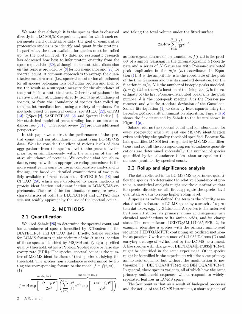
The peaks associated with a single species form a char-acteristic group, or ‘feature’, in LC-MS space. An exam-ple of such a feature is shown in Figure 1(a). Each peak inthe group collects ions of one or more isotopic forms of thespecies. The relative amplitude of the peaks measures therelative abundance of the isotopic forms. A number of soft-ware packages have been developed to detect and quantifyLC-MS features including MapQuant [19], MaxQuant [4],Sahale [25], Serac [28], SpecArray [20], and SuperHirn [26].
In tandem MS (MS/MS), selected LC-MS peaks are in-terrogated by a collision-induced dissociation (CID) and asecond MS scan recorded. Figure 1(a) displays the (t,m/z)locations (shown in red) of four MS/MS scans sampled fromthe LC-MS feature. MS/MS spectra are matched against aprotein database to determine the species from which theylikely originated. In the simplest case, the species is oneof the amino acid sequences generated by an in silico di-gest of the protein database, e.g., by trypsin. The searchspace, however, is usually expanded beyond that of the insilico digest to include, for example, species with missed ornon-tryptic cleavages, and species with altered mass due toanticipated chemical modifications of specific amino acids.Algorithms to perform this search are implemented by soft-ware packages including MyriMatch [34], Sequest [10], andX!Tandem [5]. Following identification, each spectrum-to-species match is assigned an instrument-independent qual-ity score, typically either a PeptideProphet score [17], or afalse discovery rate (FDR) calculated on the basis of hitsagainst decoy proteins in the database searched [15].
In the analysis of LC-MS/MS data, the relative abun-dance of species in a sample is generally quantified by ei-ther or both of two measures: the spectral count (see, e.g,[2, 21, 22, 37]), which is the number of MS/MS spectra iden-tified as arising from the species, or some measure of thespecies’ ion abundance derived from an analysis of its fea-ture signature in LC-MS space (see, e.g., [1, 14, 19, 28]).For example, the spectral count associated with the speciesgiving rise to the feature in Figure 1(a) is four, and one pos-sible measure of the species’ ion abundance is the volumeof the peaks fitted to its feature, as shown in Figure 1(b).Recently, the ion abundance of MS/MS spectra has beenintroduced as one component of an alternative quantitativemeasure [12]; we do not consider this measure of abundancein this work.
We note that although it is the species that is observeddirectly in a LC-MS/MS experiment, and for which such ex-periments yield quantitative data, the goal of comparativeproteomics studies is to identify and quantify the proteins.In particular, the data available for species must be ‘rolledup’ to the protein level. To date, no systematic researchhas addressed how best to infer protein quantity from thespecies quantities [30], although some statistical discussionon this topic is provided by [3] for ion abundance and [23] forspectral count. A common approach is to average the quan-titative measure used (i.e., spectral count or ion abundance)for all species belonging to a particular protein and then touse the result as a surrogate measure for the abundance ofthe protein in a statistical test. Other investigations inferrelative protein abundance directly from the abundance ofspecies, or from the abundance of species data rolled upto some intermediate level, using a variety of methods. Formethods based on spectral counts, see APEX [22], emPAI[13], QSpec [2], SASPECT [35, 36] and Spectral Index [11].For statistical models of protein rollup based on ion abun-dances, see [3, 16]. The recent review [27] provides additionalperspective.
In this paper we contrast the performance of the spec-tral count and ion abundance in quantifying LC-MS/MSdata. We also consider the effect of various levels of dataaggregation—from the species level to the protein level—prior to, or simultaneously with, the analysis of the rel-ative abundance of proteins. We conclude that ion abun-dance, coupled with an appropriate rollup procedure, is themore sensitive measure for use in comparative analysis. Ourfindings are based on detailed examinations of two pub-licly available reference data sets, BIATECH-54 [18] andCPTAC [29], which were developed to assess methods ofprotein identification and quantification in LC-MS/MS ex-periments. The use of the ion abundance measure revealscharacteristics of both the BIATECH-54 and CPTAC datasets not readily apparent by the use of the spectral count.
2. METHODS
2.1 Quantification
We used Sahale [25] to determine the spectral count andion abundance of species identified by X!Tandem in theBIATECH-54 and CPTAC data. Briefly, Sahale searchesfor LC-MS features in the vicinity of the (t,m/z) locationof those species identified by MS/MS satisfying a specifiedquality threshold, either a PeptideProphet score or false dis-covery rate (FDR). The species’ spectral count is the num-ber of MS/MS identifications of that species satisfying thethreshold. The species’ ion abundance is determined by fit-ting the corresponding feature to the model f ≡ f(t,m),(1)
f = A
model in t︷ ︸︸ ︷exp
[− (t− µ)2
2σ2
] model in m/z︷ ︸︸ ︷(N−1∑k=0
λk
k!e−λ exp
[− (m− ζk)2
2ρ2
]),
and taking the total volume under the fitted surface,
2πAσρ
N−1∑k=0
λk
k!e−λ,
as a surrogate measure of ion abundance. f(t,m) is the prod-uct of a simple Gaussian in the chromatographic (t) coordi-nate and a series of N Gaussians with Poisson-distributedpeak amplitudes in the m/z (m) coordinate. In Equa-tion (1), A is the amplitude. µ is the coordinate of the peakof the time Gaussian and σ is its standard deviation. For thefunction in m/z, N is the number of isotopic peaks modeled,ζk = ζ0+kδ is the m/z location of the kth peak, ζ0 is the co-ordinate of the first Poisson-distributed peak, k is the peaknumber, δ is the inter-peak spacing, λ is the Poisson pa-rameter, and ρ is the standard deviation of the Gaussians.Sahale fits Equation (1) to data by least squares using theLevenberg-Marquardt minimization algorithm. Figure 1(b)shows the fit determined by Sahale to the feature shown inFigure 1(a).
Sahale returns the spectral count and ion abundance forevery species for which at least one MS/MS identificationexists satisfying the quality threshold specified. Because Sa-hale quantifies LC-MS features guided by MS/MS identifica-tions, and not all the corresponding ion abundance quantifi-cations are determined successfully, the number of speciesquantified by ion abundance is less than or equal to thenumber quantified by spectral count.
2.2 Rollup and significance analysis
The data collected in an LC-MS/MS experiment quanti-fies the species. To determine the relative abundance of pro-teins, a statistical analysis might use the quantitative datafor species directly, or will first aggregate the species-levelquantitative data to some higher rollup level.
A species as we’ve defined the term is the identity asso-ciated with a feature in LC-MS space by a search of a pro-tein database, e.g., by X!Tandem. A species is characterizedby three attributes: its primary amino acid sequence, anychemical modifications to its amino acids, and its chargestate. The nomenclature DEDTQAM[147.035]PFR+2, forexample, identifies a species with the primary amino acidsequence DEDTQAMPFR containing an oxidized methion-ine at position 7 with a net mass of 147.035 Daltons (D) andcarrying a charge of +2 induced by the LC-MS instrument.A like species with charge +3, DEDTQAM[147.035]PFR+3,might be identified in the same experiment. Other speciesmight be identified in the experiment with the same primaryamino acid sequence but without the modification to me-thionine, i.e., DEDTQAMPFR+2 and DEDTQAMPFR+3.In general, these species variants, all of which have the sameprimary amino acid sequence, will correspond to widely-separated features in LC-MS space.
The key point is that as a result of biological processesand the action of the LC-MS instrument, a short segment of
2 Milac et al.
2350
2400
2450
time HsecL521.0
521.5
522.0
m�z HDL
0
5 ´ 106
1 ´ 107
(a)
2350
2400
2450
time HsecL521.0
521.5
522.0
m�z HDL
0
5 ´ 106
1 ´ 107
(b)
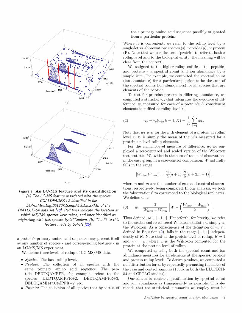
Figure 1. An LC-MS feature and its quantification.(a) The LC-MS feature associated with the species
GGALDFADFK+2 identified in file54ProtMix 1ug 051207 SampA1 01.mzXML of the
BIATECH-54 data set [18]. Red lines indicate the location atwhich MS/MS spectra were taken, and later identified as
originating with this species by X!Tandem. (b) The fit to thisfeature made by Sahale [25].
a protein’s primary amino acid sequence may present itselfas any number of species - and corresponding features - inan LC-MS/MS experiment.
We define three levels of rollup of LC-MS/MS data.
• Species: The base rollup level.• Peptide: The collection of all species with the
same primary amino acid sequence. The pep-tide DEDTQAMPFR, for example, refers to thespecies DEDTQAMPFR+2, DEDTQAMPFR+3,DEDTQAM[147.035]PFR+2, etc.
• Protein: The collection of all species that by virtue of
their primary amino acid sequence possibly originatedfrom a particular protein.
Where it is convenient, we refer to the rollup level by asingle-letter abbreviation: species (s), peptide (p), or protein(P). Note that we use the term ‘protein’ to refer to both arollup level and to the biological entity; the meaning will beclear from the context.
We assigned to the higher rollup entities - the peptidesand proteins - a spectral count and ion abundance by asimple sum. For example, we computed the spectral count(ion abundance) for a particular peptide to be the sum ofthe spectral counts (ion abundances) for all species that areelements of the peptide.
To test for proteins present in differing abundance, wecomputed a statistic, τr, that integrates the evidence of dif-ference, w, measured for each of a protein’s K constituentelements identified at rollup level r,
(2) τr = τr(wk, k = 1,K) =1
K
K∑k=1
wk.
Note that wk is w for the k’th element of a protein at rolluplevel r. τr is simply the mean of the w’s measured for aprotein’s r-level rollup elements.
For the element-level measure of difference, w, we em-ployed a zero-centered and scaled version of the Wilcoxontest statistic, W , which is the sum of ranks of observationsin the case group in a case-control comparison. W naturallyfalls in the range
[Wmin,Wmax] =[n
2(n+ 1),
n
2(n+ 2m+ 1)
],
where n and m are the number of case and control observa-tions, respectively, being compared. In our analysis, we tookthe ‘observations’ to correspond to the biological replicates.We define w as
(3) w =2
Wmax −Wmin
[W −
(Wmax +Wmin
2
)].
Thus defined, w ∈ [−1, 1]. Henceforth, for brevity, we referto the scaled and re-centered Wilcoxon statistic w simply asthe Wilcoxon. As a consequence of the definition of w, τr,defined in Equation (2), falls in the range [−1, 1] indepen-dently of K. Note that at the protein level of rollup, K = 1and τP = w, where w is the Wilcoxon computed for theprotein at the protein level of rollup.
We computed τr using both the spectral count and ionabundance measures for all elements at the species, peptideand protein rollup levels. To derive p-values, we computed anull distribution for τr by repeatedly permuting the labels ofthe case and control samples (1500x in both the BIATECH-54 and CPTAC studies).
Our aim is to contrast quantification by spectral countand ion abundance as transparently as possible. This de-mands that the statistical summaries we employ must be
Analyzing by spectral count and ion abundance 3
comparable and based on the same concepts. The statisticτr is simply the average of Wilcoxon test statistics for a pro-tein’s constituent elements at a given rollup level, computedin the same way at each level using the spectral count or theion abundance.
3. CASE STUDIES
3.1 BIATECH-54
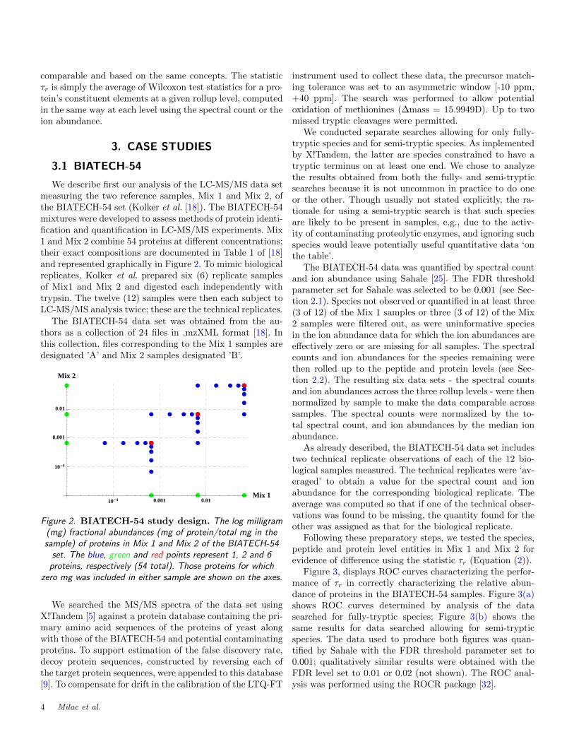
We describe first our analysis of the LC-MS/MS data setmeasuring the two reference samples, Mix 1 and Mix 2, ofthe BIATECH-54 set (Kolker et al. [18]). The BIATECH-54mixtures were developed to assess methods of protein identi-fication and quantification in LC-MS/MS experiments. Mix1 and Mix 2 combine 54 proteins at different concentrations;their exact compositions are documented in Table 1 of [18]and represented graphically in Figure 2. To mimic biologicalreplicates, Kolker et al. prepared six (6) replicate samplesof Mix1 and Mix 2 and digested each independently withtrypsin. The twelve (12) samples were then each subject toLC-MS/MS analysis twice; these are the technical replicates.
The BIATECH-54 data set was obtained from the au-thors as a collection of 24 files in .mzXML format [18]. Inthis collection, files corresponding to the Mix 1 samples aredesignated ’A’ and Mix 2 samples designated ’B’.
10-4 0.001 0.01Mix 1
10-4
0.001
0.01
Mix 2
Figure 2. BIATECH-54 study design. The log milligram(mg) fractional abundances (mg of protein/total mg in thesample) of proteins in Mix 1 and Mix 2 of the BIATECH-54
set. The blue, green and red points represent 1, 2 and 6proteins, respectively (54 total). Those proteins for which
zero mg was included in either sample are shown on the axes.
We searched the MS/MS spectra of the data set usingX!Tandem [5] against a protein database containing the pri-mary amino acid sequences of the proteins of yeast alongwith those of the BIATECH-54 and potential contaminatingproteins. To support estimation of the false discovery rate,decoy protein sequences, constructed by reversing each ofthe target protein sequences, were appended to this database[9]. To compensate for drift in the calibration of the LTQ-FT
instrument used to collect these data, the precursor match-ing tolerance was set to an asymmetric window [-10 ppm,+40 ppm]. The search was performed to allow potentialoxidation of methionines (∆mass = 15.9949D). Up to twomissed tryptic cleavages were permitted.
We conducted separate searches allowing for only fully-tryptic species and for semi-tryptic species. As implementedby X!Tandem, the latter are species constrained to have atryptic terminus on at least one end. We chose to analyzethe results obtained from both the fully- and semi-trypticsearches because it is not uncommon in practice to do oneor the other. Though usually not stated explicitly, the ra-tionale for using a semi-tryptic search is that such speciesare likely to be present in samples, e.g., due to the activ-ity of contaminating proteolytic enzymes, and ignoring suchspecies would leave potentially useful quantitative data ‘onthe table’.
The BIATECH-54 data was quantified by spectral countand ion abundance using Sahale [25]. The FDR thresholdparameter set for Sahale was selected to be 0.001 (see Sec-tion 2.1). Species not observed or quantified in at least three(3 of 12) of the Mix 1 samples or three (3 of 12) of the Mix2 samples were filtered out, as were uninformative speciesin the ion abundance data for which the ion abundances areeffectively zero or are missing for all samples. The spectralcounts and ion abundances for the species remaining werethen rolled up to the peptide and protein levels (see Sec-tion 2.2). The resulting six data sets - the spectral countsand ion abundances across the three rollup levels - were thennormalized by sample to make the data comparable acrosssamples. The spectral counts were normalized by the to-tal spectral count, and ion abundances by the median ionabundance.
As already described, the BIATECH-54 data set includestwo technical replicate observations of each of the 12 bio-logical samples measured. The technical replicates were ‘av-eraged’ to obtain a value for the spectral count and ionabundance for the corresponding biological replicate. Theaverage was computed so that if one of the technical obser-vations was found to be missing, the quantity found for theother was assigned as that for the biological replicate.
Following these preparatory steps, we tested the species,peptide and protein level entities in Mix 1 and Mix 2 forevidence of difference using the statistic τr (Equation (2)).
Figure 3, displays ROC curves characterizing the perfor-mance of τr in correctly characterizing the relative abun-dance of proteins in the BIATECH-54 samples. Figure 3(a)shows ROC curves determined by analysis of the datasearched for fully-tryptic species; Figure 3(b) shows thesame results for data searched allowing for semi-trypticspecies. The data used to produce both figures was quan-tified by Sahale with the FDR threshold parameter set to0.001; qualitatively similar results were obtained with theFDR level set to 0.01 or 0.02 (not shown). The ROC anal-ysis was performed using the ROCR package [32].
4 Milac et al.
False positive rate
True
pos
itive
rat
e
0.0 0.2 0.4 0.6 0.8 1.0
0.0
0.2
0.4
0.6
0.8
1.0
species (0.84) " (0.77)peptide (0.84) " (0.77)protein (0.76) " (0.78)
(a)
False positive rate
True
pos
itive
rat
e
0.0 0.2 0.4 0.6 0.8 1.0
0.0
0.2
0.4
0.6
0.8
1.0
species (0.69) " (0.76)peptide (0.54) " (0.8)protein (0.81) " (0.79)
(b)
Figure 3. ROC comparison of performance. ROCcurves showing the performance of τr, computed using the
spectral count (dotted) and ion abundance (solid) measures,in characterizing the relative abundance of proteins in Mix 1
and Mix 2 of the BIATECH-54 set across the species, peptideand protein rollup levels. (a) shows the results obtained using
the data searched for fully-tryptic species, and (b) forsemi-tryptic species. The AUC corresponding to each curve is
shown in parenthesis.
In Figure 3(a), we see that at the species and peptidelevels the AUC computed using the ion abundance is ap-proximately 9% higher than that obtained using the spec-
tral count; the AUCs are approximately equal at the proteinlevel. The ion abundance at the protein level, however, yieldsan AUC appreciably less than that at the species and pep-tide levels. By contrast, the spectral count yields an AUCthat is nearly constant across rollup levels.
Using the semi-tryptic data, the relative performance ofthe spectral count and ion abundance is nearly reversed(Figure 3(b)). Strikingly, the performance of ion abundanceat the species and peptide rollup levels is significantly lowerthan that obtained using the fully-tryptic data whereas theperformance at the protein level is nearly the same. Withthe semi-tryptic data, as with the fully-tryptic, the perfor-mance of the spectral count is relatively consistent acrossrollup levels and approximately equal to the AUCs com-puted using the fully-tryptic data.
Initially, we were puzzled by these findings, particularlyby the disparity of performance, between the fully-trypticand semi-tryptic data, of ion abundance at the species andpeptide levels of rollup. Also confusing is that the perfor-mance of ion abundance at the protein level of rollup inthe semi-tryptic data ‘recovers’ to that obtained with thefully-tryptic data.
A further examination revealed that these findings reflectan actual difference between the Mix 1 and Mix 2 samples ofthe BIATECH-54 set not detected using the spectral count.Figure 4(a) shows the total number of strictly semi-trypticspecies (i.e., not fully-tryptic) detected in each of the 24samples of the BIATECH-54 data set. Clearly, strictly semi-tryptic species are observed more frequently in the Mix 1than in the Mix 2 samples. We believe this fact reflects adifference in the way in which the samples themselves wereprepared; a contaminating (non-trypsin) proteolytic enzymemay have been introduced into the Mix 1 samples, or mayhave been more active in these than in the Mix 2 samples.
This difference between the Mix 1 and Mix 2 samplesis manifest in the ROC plots for the semi-tryptic data be-cause the structure of τr as an average of Wilcoxon statisticsmakes it sensitive to the contributions made by the addi-tional strictly semi-tryptic species observed in Mix 1. Forτs, for example, each observation of a strictly semi-trypticspecies in Mix 1 that is not in Mix 2 makes an incrementalcontribution that carries equal weight to the contributionsmade by species observed in both samples.
Figure 4(b) shows the fraction of ion abundance con-tributed by the strictly semi-tryptic species in the 24 sam-ples. Despite the fact that more strictly semi-tryptic speciesare present in Mix 1 than in Mix 2, their relative contri-bution to the total ion abundance in each sample is nearlyequal across samples. This suggests that the ion abundancesignal associated with strictly semi-tryptic species is small.It also explains the ‘recovery’ of performance observed inFigure 3(b) for data analyzed at the protein rollup level.Rollup to the protein level ‘hides’ the relatively small con-tribution made to each protein’s total ion abundance by thelow-abundance strictly semi-tryptic species.
Analyzing by spectral count and ion abundance 5
Sample
Tota
l num
ber
of s
tric
tly s
emi−
tryp
tic s
peci
es o
bser
ved
150
200
250
A1_
01
A1_
02
A2_
01
A2_
02
A3_
01
A3_
02
A4_
01
A4_
02
A5_
01
A5_
02
A6_
01
A6_
02
B1_
01
B1_
02
B2_
01
B2_
02
B3_
01
B3_
02
B4_
01
B4_
02
B5_
01
B5_
02
B6_
01
B6_
02
(a)
Sample
Fra
ctio
n of
ion
abun
danc
e co
ntrib
uted
by
stric
tly s
emi−
tryp
tic s
peci
es
0.0
0.1
0.2
0.3
0.4
A1_
01
A1_
02
A2_
01
A2_
02
A3_
01
A3_
02
A4_
01
A4_
02
A5_
01
A5_
02
A6_
01
A6_
02
B1_
01
B1_
02
B2_
01
B2_
02
B3_
01
B3_
02
B4_
01
B4_
02
B5_
01
B5_
02
B6_
01
B6_
02
(b)
Figure 4. Strictly semi-tryptic species content byexperiment. (a) Strictly semi-tryptic species are observed
more frequently in the Mix 1 (A) than in the Mix 2 (B)samples of the BIATECH-54 data set, searched to permit theobservation of such species. (b) The fraction of the total ionabundance contributed by strictly semi-tryptic species varies
little between the Mix 1 and Mix 2 samples.
It is more difficult to provide a simple explanation for
the poor performance seen in Figure 3(b) for the interme-
diate, peptide level of rollup. The performance is the re-
sult of a complex interaction of two factors: the number ofspecies that contribute to the quantification of each peptide;and the relative contribution made by the additional strictlysemi-tryptic species observed in the Mix 1 samples to thequantification of each peptide.
Using a semi-tryptic search strategy and the ion abun-dance measure, we’ve found that the BIATECH-54 samplesMix 1 and Mix 2 differ markedly in their content of strictlysemi-tryptic species (Figure 4(a)). We detected this anomalyat the species and peptide levels of rollup, but not at theprotein level (Figure 3(b)), using our Wilcoxon rank-sum-based test. The same analysis carried out using the spectralcount measure gave no hint of this unanticipated finding.Our analysis suggests not only that the ion abundance is amore sensitive measure of quantification than is the spec-tral count, but that analysis of LC-MS/MS data at differentlevels of rollup can be informative.
3.2 CPTAC
In a study conducted by the Clinical Proteomic Tech-nologies for Cancer (CPTAC) consortium, Paulovich et al.[29] introduced a reference data set measuring new perfor-mance standards for benchmarking of LC-MS/MS platformsand data analysis methods. These new standards are basedon the yeast proteome and the UPS1 (Universal ProteomcsStandard Set 1) collection of 48 human source or humansequence recombinant proteins [31]. The CPTAC referencesamples and data set therefore provide a more complex andchallenging benchmark for LC-MS/MS analysis than doesBIATECH-54.
Table 1. The composition of the CPTAC samples.
Sample Yeast UPS1 (Sigma-48)(ng/µL) (fmol/µL)
QC2 60 0A 60 0.25B 60 0.74C 60 2.2D 60 6.7E 60 20
We analzyed a subset of the data collected for the CPTACstudy, comparing the trypsin-digested yeast protein lysatesamples, designated QC2, with the UPS1 spike-in samples,designated A, B, C, D and E. The composition of thesesamples is summarized in Table 1, which is excerpted fromSection C of [29, Supplementary Information]. The four lab-oratories participating in the study each collected three tech-nical replicate observations of the QC2, A, B, C, D and Esamples for a total of twelve (12) observations of each.
The MS/MS spectra were searched using X!Tandemagainst the same protein database used by the CPTAC au-thors, which includes both target and decoy (reversed) pro-tein sequences. The precursor matching tolerance was set to
6 Milac et al.
Table 2. The number of yeast and UPS1 proteins found to bepresent in greater (⇑) and lesser (⇓) abundance in samplesA-E relative to QC2 of the CPTAC data at FDR level 0.05.
[-10 ppm, +10 ppm]. The search was performed to allow forpotential oxidation of methionines (∆m = 15.9949D) andcarbamidomethylation of cysteines (∆m = 57.0215D). Upto two missed tryptic cleavages were permitted. The searchwas conducted allowing for only fully-tryptic species.
The CPTAC data was quantified by spectral count andion abundance using Sahale executed with the FDR thresh-old parameter set to 0.001. Species not observed or quan-tified in at least three (3 of 12) of the A, B, C, D or Esamples or three (3 of 12) of the QC2 samples were filteredout, as were uninformative species in the ion abundance datafor which the ion abundances were effectively zero or weremissing for all samples. The data was then rolled up. Thespectral counts in each sample were normalized by the totalspectral count, and the ion abundances by the median ionabundance.
Following these preparatory steps, we searched for pro-teins present in differing abundance in the QC2 and A, B,C, D or E samples using the statistic τr (Equation (2)) com-puted at the species, peptide and protein rollup levels. Fol-lowing the methodology used by Paulovich et al. [29] in the
analysis leading to their Table III, we treated the 12 observa-tions of each sample type as biological replicates. Note thatbecause we tested on the rank computed for the QC2 sam-ples, species, peptide or protein elements less abundant inthe A-E samples than in QC2 have w > 0. This observationwill be important in the following.
p−value
Den
sity
0
1
2
3
0.2 0.4 0.6 0.8
Spectral countACE
p−value
Den
sity
0
1
2
3
0.2 0.4 0.6 0.8
Ion abundanceACE
Figure 5. Stratified p-values for yeast proteins.Density estimate of the distribution of ps for yeast proteinsonly of the A, C and E samples, tested against QC2, of the
CPTAC data set.
To correct for the effects of multiple hypothesis testing,we converted p-values to false discovery rates using the Rpackage qvalue (see [33]). The numbers of yeast and UPS1proteins found to be present in greater and lesser abundancein samples A-E relative to QC2 at FDR level 0.05 are shownin Table 2.
Table 2 shows that the performance of the spectral countis somewhat better than ion abundance in correctly char-acterizing the abundance of the UPS1 proteins in the casesamples across rollup levels, particularly at the lower levelsof spike-in. However, what stands out in Table 2 is the largenumber of yeast proteins found to have different abundancein the E and QC2 samples. The number of these apparentfalse positives is particularly high in the results computedusing ion abundance. We sought to understand the origin ofthese ’false positives’, initially suspecting some error in themethod by which features were quantified by ion abundance.
Figure 5 shows the distribution of p-values computed forthe yeast proteins only of the A, C and E samples. These p-values were computed on the basis of τs, that is, on the basisof the spectral counts and ion abundances at the specieslevel of rollup. Figure 5 shows that the proportion of yeastproteins determined to be significant increases as a function
Analyzing by spectral count and ion abundance 7
of increasing UPS1 protein concentration. This is the casefor p-values computed using either the spectral count or ionabundance measure, though the trend is more easily seen inthe ion abundance results.
τs
Den
sity
0
1
2
3
−0.5 0.0 0.5
A vs. QC2Spectral countIon abundance
τs
Den
sity
0
1
2
3
−0.5 0.0 0.5
C vs. QC2Spectral countIon abundance
τs
Den
sity
0
1
2
3
−0.5 0.0 0.5
E vs. QC2Spectral countIon abundance
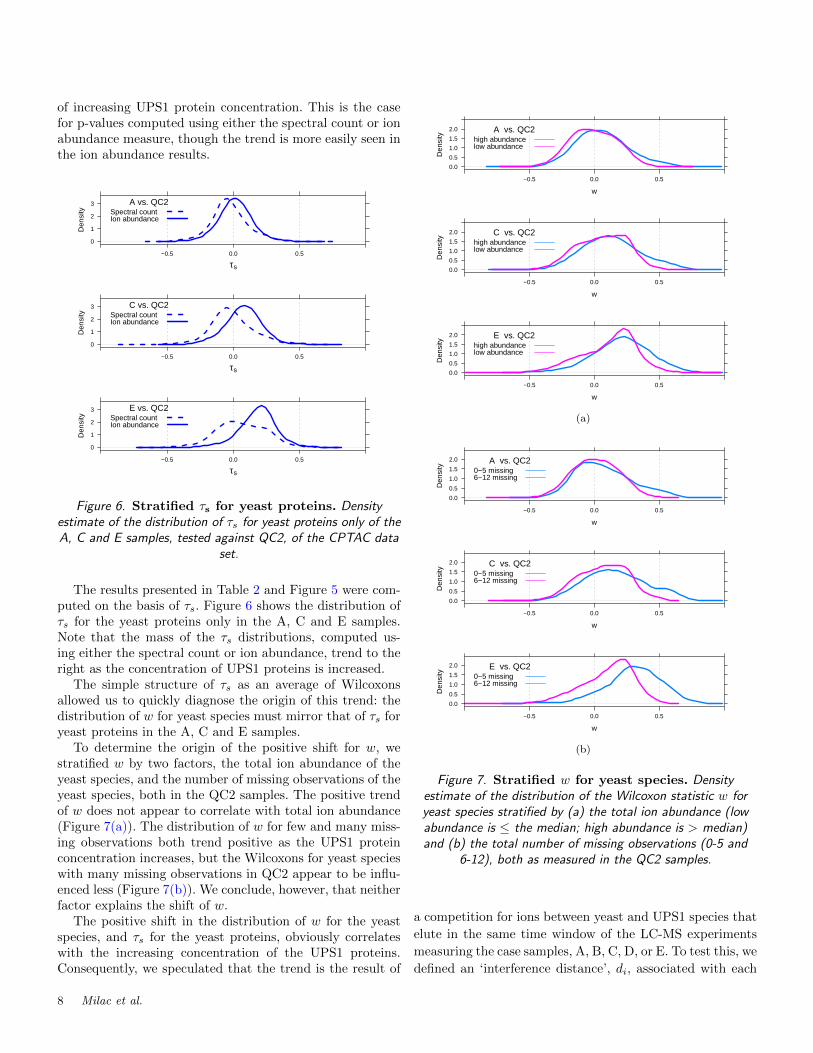
Figure 6. Stratified τs for yeast proteins. Densityestimate of the distribution of τs for yeast proteins only of theA, C and E samples, tested against QC2, of the CPTAC data
set.
The results presented in Table 2 and Figure 5 were com-puted on the basis of τs. Figure 6 shows the distribution ofτs for the yeast proteins only in the A, C and E samples.Note that the mass of the τs distributions, computed us-ing either the spectral count or ion abundance, trend to theright as the concentration of UPS1 proteins is increased.
The simple structure of τs as an average of Wilcoxonsallowed us to quickly diagnose the origin of this trend: thedistribution of w for yeast species must mirror that of τs foryeast proteins in the A, C and E samples.
To determine the origin of the positive shift for w, westratified w by two factors, the total ion abundance of theyeast species, and the number of missing observations of theyeast species, both in the QC2 samples. The positive trendof w does not appear to correlate with total ion abundance(Figure 7(a)). The distribution of w for few and many miss-ing observations both trend positive as the UPS1 proteinconcentration increases, but the Wilcoxons for yeast specieswith many missing observations in QC2 appear to be influ-enced less (Figure 7(b)). We conclude, however, that neitherfactor explains the shift of w.
The positive shift in the distribution of w for the yeastspecies, and τs for the yeast proteins, obviously correlateswith the increasing concentration of the UPS1 proteins.Consequently, we speculated that the trend is the result of
w
Den
sity
0.0
0.5
1.0
1.5
2.0
−0.5 0.0 0.5
A vs. QC2high abundancelow abundance
w
Den
sity
0.0
0.5
1.0
1.5
2.0
−0.5 0.0 0.5
C vs. QC2high abundancelow abundance
w
Den
sity
0.0
0.5
1.0
1.5
2.0
−0.5 0.0 0.5
E vs. QC2high abundancelow abundance
(a)
w
Den
sity
0.0
0.5
1.0
1.5
2.0
−0.5 0.0 0.5
A vs. QC20−5 missing6−12 missing
w
Den
sity
0.0
0.5
1.0
1.5
2.0
−0.5 0.0 0.5
C vs. QC20−5 missing6−12 missing
w
Den
sity
0.0
0.5
1.0
1.5
2.0
−0.5 0.0 0.5
E vs. QC20−5 missing6−12 missing
(b)
Figure 7. Stratified w for yeast species. Densityestimate of the distribution of the Wilcoxon statistic w foryeast species stratified by (a) the total ion abundance (lowabundance is ≤ the median; high abundance is > median)and (b) the total number of missing observations (0-5 and
6-12), both as measured in the QC2 samples.
a competition for ions between yeast and UPS1 species that
elute in the same time window of the LC-MS experiments
measuring the case samples, A, B, C, D, or E. To test this, we
defined an ‘interference distance’, di, associated with each
8 Milac et al.
i = 1
i = 2
j = 1
j = 2
Sample k
m/z
(D)
time (sec)
UPS1 feature
Yeast feature
d21k > 0
d11k = 0
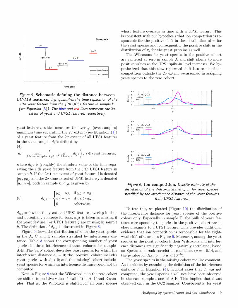
Figure 8. Schematic defining the distance betweenLC-MS features. dijk quantifies the time separation of thei’th yeast feature from the j’th UPS1 feature in sample k
(see Equation (5)). The blue and red lines represent the 2σextent of yeast and UPS1 features, respectively.
yeast feature i, which measures the average (over samples)minimum time separating the 2σ extent (see Equation (1))of a yeast feature from the 2σ extent of all UPS1 featuresin the same sample. di is defined by(4)
di = meank∈case samples
(min
j∈UPS1 featuredijk
), i ∈ yeast features,
where dijk is (roughly) the absolute value of the time sepa-rating the i’th yeast feature from the j’th UPS1 feature insample k. If the 2σ time extent of yeast feature i is denoted[yL, yR], and the 2σ time extent of UPS1 feature j is denoted[uL, uR], both in sample k, dijk is given by
(5) dijk =
yL − uR if yL > uR,
uL − yR if uL > yR,
0 otherwise.
dijk = 0 when the yeast and UPS1 features overlap in timeand potentially compete for ions; dijk is taken as missing ifthe yeast feature i or UPS1 feature j are missing in samplek. The definition of dijk is illustrated in Figure 8.
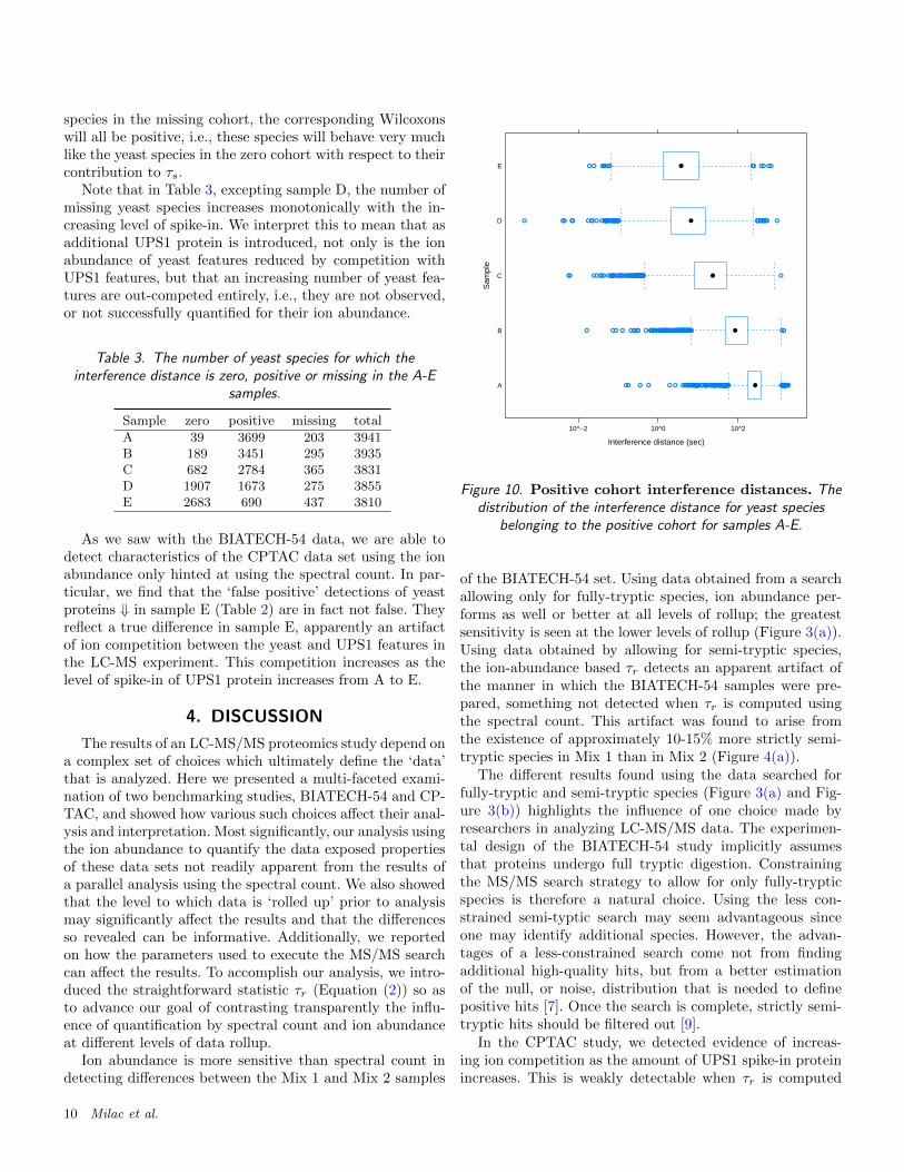
Figure 9 shows the distribution of w for the yeast speciesin the A, C and E samples stratified by interference dis-tance. Table 3 shows the corresponding number of yeastspecies in three interference distance cohorts for samplesA-E. The ‘zero’ cohort describes yeast species for which theinterference distance di = 0; the ‘positive’ cohort includesyeast species with di > 0; and the ‘missing’ cohort includesyeast species for which an interference distance could not becomputed.
Note in Figure 9 that the Wilcoxons w in the zero cohortare shifted to positive values for all of the A, C and E sam-ples. That is, the Wilcoxon is shifted for all yeast species
whose feature overlaps in time with a UPS1 feature. Thisis consistent with our hypothesis that ion competition is re-sponsible for the positive shift in the distribution of w forthe yeast species and, consequently, the positive shift in thedistribution of τs for the yeast proteins as well.
The Wilcoxons for yeast species in the positive cohortare centered at zero in sample A and shift slowly to morepositive values as the UPS1 spike-in level increases. We hy-pothesized that this slow rightward shift is a result of ioncompetition outside the 2σ extent we assumed in assigningyeast species to the zero cohort.
w
Den
sity
0
1
2
3
4
−0.5 0.0 0.5
A vs. QC2positivezero
w
Den
sity
0
1
2
3
4
−0.5 0.0 0.5
C vs. QC2positivezero
w
Den
sity
0
1
2
3
4
−0.5 0.0 0.5
E vs. QC2positivezero
Figure 9. Ion competition. Density estimate of thedistribution of the Wilcoxon statistic, w, for yeast speciesstratified by the interference distance of the yeast features
from UPS1 features.
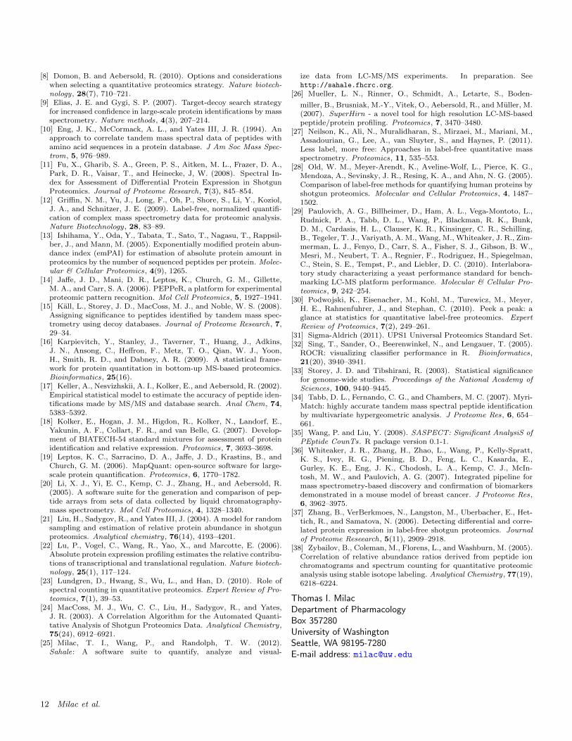
To test this, we plotted (Figure 10) the distribution ofthe interference distance for yeast species of the positivecohort only. Especially in sample E, the bulk of yeast fea-tures corresponding to species in the positive cohort are inclose proximity to a UPS1 feature. This provides additionalevidence that ion competition is responsible for the right-ward shift of w seen in Figure 9. Moreover, among the yeastspecies in the positive cohort, their Wilcoxons and interfer-ence distances are significantly negatively correlated, basedon Spearman’s rank correlation coefficient (ρ = −0.14, andthe p-value for H0 : ρ = 0 is < 10−5).
The yeast species in the missing cohort require comment.As is evident by examining the definition of the interferencedistance di in Equation (4), in most cases that di was notcomputed, the yeast species i will not have been observedin the case samples, one of A-E. This implies that i wasobserved only in the QC2 samples. Consequently, for yeast
Analyzing by spectral count and ion abundance 9
species in the missing cohort, the corresponding Wilcoxonswill all be positive, i.e., these species will behave very muchlike the yeast species in the zero cohort with respect to theircontribution to τs.
Note that in Table 3, excepting sample D, the number ofmissing yeast species increases monotonically with the in-creasing level of spike-in. We interpret this to mean that asadditional UPS1 protein is introduced, not only is the ionabundance of yeast features reduced by competition withUPS1 features, but that an increasing number of yeast fea-tures are out-competed entirely, i.e., they are not observed,or not successfully quantified for their ion abundance.
Table 3. The number of yeast species for which theinterference distance is zero, positive or missing in the A-E
As we saw with the BIATECH-54 data, we are able todetect characteristics of the CPTAC data set using the ionabundance only hinted at using the spectral count. In par-ticular, we find that the ‘false positive’ detections of yeastproteins ⇓ in sample E (Table 2) are in fact not false. Theyreflect a true difference in sample E, apparently an artifactof ion competition between the yeast and UPS1 features inthe LC-MS experiment. This competition increases as thelevel of spike-in of UPS1 protein increases from A to E.
4. DISCUSSION
The results of an LC-MS/MS proteomics study depend ona complex set of choices which ultimately define the ‘data’that is analyzed. Here we presented a multi-faceted exami-nation of two benchmarking studies, BIATECH-54 and CP-TAC, and showed how various such choices affect their anal-ysis and interpretation. Most significantly, our analysis usingthe ion abundance to quantify the data exposed propertiesof these data sets not readily apparent from the results ofa parallel analysis using the spectral count. We also showedthat the level to which data is ‘rolled up’ prior to analysismay significantly affect the results and that the differencesso revealed can be informative. Additionally, we reportedon how the parameters used to execute the MS/MS searchcan affect the results. To accomplish our analysis, we intro-duced the straightforward statistic τr (Equation (2)) so asto advance our goal of contrasting transparently the influ-ence of quantification by spectral count and ion abundanceat different levels of data rollup.
Ion abundance is more sensitive than spectral count indetecting differences between the Mix 1 and Mix 2 samples
Figure 10. Positive cohort interference distances. Thedistribution of the interference distance for yeast species
belonging to the positive cohort for samples A-E.
of the BIATECH-54 set. Using data obtained from a searchallowing only for fully-tryptic species, ion abundance per-forms as well or better at all levels of rollup; the greatestsensitivity is seen at the lower levels of rollup (Figure 3(a)).Using data obtained by allowing for semi-tryptic species,the ion-abundance based τr detects an apparent artifact ofthe manner in which the BIATECH-54 samples were pre-pared, something not detected when τr is computed usingthe spectral count. This artifact was found to arise fromthe existence of approximately 10-15% more strictly semi-tryptic species in Mix 1 than in Mix 2 (Figure 4(a)).
The different results found using the data searched forfully-tryptic and semi-tryptic species (Figure 3(a) and Fig-ure 3(b)) highlights the influence of one choice made byresearchers in analyzing LC-MS/MS data. The experimen-tal design of the BIATECH-54 study implicitly assumesthat proteins undergo full tryptic digestion. Constrainingthe MS/MS search strategy to allow for only fully-trypticspecies is therefore a natural choice. Using the less con-strained semi-typtic search may seem advantageous sinceone may identify additional species. However, the advan-tages of a less-constrained search come not from findingadditional high-quality hits, but from a better estimationof the null, or noise, distribution that is needed to definepositive hits [7]. Once the search is complete, strictly semi-tryptic hits should be filtered out [9].
In the CPTAC study, we detected evidence of increas-ing ion competition as the amount of UPS1 spike-in proteinincreases. This is weakly detectable when τr is computed
10 Milac et al.
using the spectral count but is obvious when the ion abun-dance is used; see Table 2 and the companion perspectivesin Figures 5 and 6. The sample-dependent trends seen inthese figures reveals that the abundance of yeast proteinsdecreases as a function of increasing UPS1 spike-in. Con-ceivably, this was an artifact of a quantification method thattreated high/low abundance or missing features differently.However, by stratifying the Wilcoxon w on low-versus-hightotal ion abundance and on few-versus-many missing obser-vations of yeast species in QC2 (Figure 7), we diagnosedthat this is not the case. The existence of ion competition inthe CPTAC data was confirmed by stratifying the Wilcoxonstatistics for yeast species on the basis of their interferencedistance (see Figures 9 and 10).
Our findings for the CPTAC data raises the question asto whether the spike-in experimental design is appropriatefor the construction of a benchmark case-control study. Thevery introduction of a spike-in appears to bias the data byion competition. Possibly, the bias we detect is a conse-quence of ‘too much’ UPS1 protein having been introduced,in the E sample in particular. However, a simple calculationconfirms that the average mass of yeast protein per µl ofE sample exceeds that for an average UPS1 protein by ap-proximately 20% (1.1×10⁻¹¹ grams per UPS1 protein versus1.33× 10−11 grams per yeast protein, assuming ∼4,500 ex-pressed yeast proteins [29]). This suggests that one must becautious in interpreting the results obtained from a label-free LC-MS/MS experiment, as an over-expressed collectionof proteins may interfere with the ion signal measured forother classes.
Our findings differ somewhat from those of Zybailov etal. [38] who conclude that the spectral count is more re-liable than ion abundance (as summarized by the RelExmethod of MacCoss et al. [24]). Similarly, Old et al. [28]conclude that the spectral count is more sensitive than ionabundance (as summarized by Serac) in detecting differen-tially expressed proteins. On the other hand, that study alsoobserves that the ion abundance yields more accurate esti-mates of protein ratios than does the spectral count andso no definitive conclusion was drawn. We note that Oldet al. use one statistic for spectral count data and anotherstatistic for ion abundance data and so it is difficult to com-pare their results to ours. Indeed, comparison between spec-tral count and ion abundance is complicated by the myriadways in which MS and MS/MS data are quantified and sum-marized statistically. This is an important point: neither ofthe terms “spectral count” nor “ion abundance” refers to awell-defined quantification method but rather to a generalapproach used to define quantities that enter into the statis-tical analysis. Not only are there many ways to define thesequantities but there are also many ways to define the statis-tics that ultimately summarize protein comparisons, as seenin our discussion of peptide “rollup”.
In our analyses, we have attempted to ensure that anydifferences observed when using spectral count versus ion
abundance for quantification are not due to non-comparableaspects of the analysis. Our use of the Wilcoxon in definingτr for both measures of quantification at each level of rollupallows for a statistically even-handed comparison. Addition-ally, the MS/MS-directed approach we employed to quan-tify ion abundance ensures the fairness of the comparisonwe make between the spectral count and ion abundance asthis approach quantifies the same set of CIDs in each case.
We note in passing that we investigated a variant of τrcomputed using the t-statistic. We found the performanceof this variant is less attractive than that based on theWilcoxon. This is a consequence of the small sample sizeof the case studies and the parametric assumptions under-lying the use of the t-statistic.
Finally, there are a variety of reasons to favor ion abun-dance for quantification. The statistical models for proteinrollup by Clough et al. [3], for example, are implicitly basedon ion abundances. Also, as noted by Podwojski et al. [30]and Lundgren et al. [23], spectral counts may be dominatedby a few proteins having a large number of counts, and thespectral count breaks down as a statistical quantity whenvery few counts are observed. Although the estimated ionabundance of an identified species is subject to low signaland the stochastic nature of the CID sampling, it has thepotential to more robustly quantify seldom-seen species.
ACKNOWLEDGEMENTS
The authors thank Jason Hogan and Matthew Fitzgib-bon for their assistance in preparing the BIATECH-54 andCPTAC data for analysis.
Funding: This work was supported by NIH grants R21RR025787 (TR,TM), R01 CA126205 (TR,TM,PW), R01GM082802 (PW,TR) and U01 CA086368 (TR).
REFERENCES
[1] Bondarenko, P., Chelius, D., and Shaler, T. (2002). Identificationand relative quantitation of protein mixtures by enzymatic digestionfollowed by capillary reversed-phase liquid chromatography-tandemmass spectrometry. Analytical chemistry, 74(18), 4741–4749.
[2] Choi, H., Fermin, D., and Nesvizhskii, A. I. (2008). Significanceanalysis of spectral count data in label-free shotgun proteomics. MolCell Proteomics, 7, 2373–2385.
[3] Clough, T., Key, M., Ott, I., Ragg, S., Schadow, G., and Vitek,O. (2009). Protein quantification in label-free LC-MS experiments.Journal of Proteome Research, 8, 5275–5284.
[4] Cox, J. and Mann, M. (2008). MaxQuant enables high peptideidentification rates, individualized p.p.b-range mass accuracies andproteome-wide protein quantification. Nature Biotechnology, 26,1367–1372.
[5] Craig, R. and Beavis, R. C. (2004). TANDEM: matching proteinswith tandem mass spectra. Bioinformatics, 20, 1466–1467.
[6] Deutsch, E. W., Lam, H., and Aebersold, R. (2008). Data analy-sis and bioinformatics tools for tandem mass spectrometry in pro-teomics. Physiological genomics, 33(1), 18–25.
[7] Ding, Y., Choi, H., and Nesvizhskii, A. I. (2008). Adaptive discrim-inant function analysis and reranking of MS/MS database searchresults for improved peptide identification in shotgun proteomics.Journal of Proteome Research, 7(11), 4878–4889.
Analyzing by spectral count and ion abundance 11
[8] Domon, B. and Aebersold, R. (2010). Options and considerationswhen selecting a quantitative proteomics strategy. Nature biotech-nology, 28(7), 710–721.
[9] Elias, J. E. and Gygi, S. P. (2007). Target-decoy search strategyfor increased confidence in large-scale protein identifications by massspectrometry. Nature methods, 4(3), 207–214.
[10] Eng, J. K., McCormack, A. L., and Yates III, J. R. (1994). Anapproach to correlate tandem mass spectral data of peptides withamino acid sequences in a protein database. J Am Soc Mass Spec-trom, 5, 976–989.
[11] Fu, X., Gharib, S. A., Green, P. S., Aitken, M. L., Frazer, D. A.,Park, D. R., Vaisar, T., and Heinecke, J, W. (2008). Spectral In-dex for Assessment of Differential Protein Expression in ShotgunProteomics. Journal of Proteome Research, 7(3), 845–854.
[12] Griffin, N. M., Yu, J., Long, F., Oh, P., Shore, S., Li, Y., Koziol,J. A., and Schnitzer, J. E. (2009). Label-free, normalized quantifi-cation of complex mass spectrometry data for proteomic analysis.Nature Biotechnology, 28, 83–89.
[13] Ishihama, Y., Oda, Y., Tabata, T., Sato, T., Nagasu, T., Rappsil-ber, J., and Mann, M. (2005). Exponentially modified protein abun-dance index (emPAI) for estimation of absolute protein amount inproteomics by the number of sequenced peptides per protein. Molec-ular & Cellular Proteomics, 4(9), 1265.
[14] Jaffe, J. D., Mani, D. R., Leptos, K., Church, G. M., Gillette,M. A., and Carr, S. A. (2006). PEPPeR, a platform for experimentalproteomic pattern recognition. Mol Cell Proteomics, 5, 1927–1941.
[15] Kall, L., Storey, J. D., MacCoss, M. J., and Noble, W. S. (2008).Assigning significance to peptides identified by tandem mass spec-trometry using decoy databases. Journal of Proteome Research, 7,29–34.
[16] Karpievitch, Y., Stanley, J., Taverner, T., Huang, J., Adkins,J. N., Ansong, C., Heffron, F., Metz, T. O., Qian, W. J., Yoon,H., Smith, R. D., and Dabney, A. R. (2009). A statistical frame-work for protein quantitation in bottom-up MS-based proteomics.Bioinformatics, 25(16).
[17] Keller, A., Nesvizhskii, A. I., Kolker, E., and Aebersold, R. (2002).Empirical statistical model to estimate the accuracy of peptide iden-tifications made by MS/MS and database search. Anal Chem, 74,5383–5392.
[18] Kolker, E., Hogan, J. M., Higdon, R., Kolker, N., Landorf, E.,Yakunin, A. F., Collart, F. R., and van Belle, G. (2007). Develop-ment of BIATECH-54 standard mixtures for assessment of proteinidentification and relative expression. Proteomics, 7, 3693–3698.
[19] Leptos, K. C., Sarracino, D. A., Jaffe, J. D., Krastins, B., andChurch, G. M. (2006). MapQuant: open-source software for large-scale protein quantification. Proteomics, 6, 1770–1782.
[20] Li, X. J., Yi, E. C., Kemp, C. J., Zhang, H., and Aebersold, R.(2005). A software suite for the generation and comparison of pep-tide arrays from sets of data collected by liquid chromatography-mass spectrometry. Mol Cell Proteomics, 4, 1328–1340.
[21] Liu, H., Sadygov, R., and Yates III, J. (2004). A model for randomsampling and estimation of relative protein abundance in shotgunproteomics. Analytical chemistry, 76(14), 4193–4201.
[22] Lu, P., Vogel, C., Wang, R., Yao, X., and Marcotte, E. (2006).Absolute protein expression profiling estimates the relative contribu-tions of transcriptional and translational regulation. Nature biotech-nology, 25(1), 117–124.
[23] Lundgren, D., Hwang, S., Wu, L., and Han, D. (2010). Role ofspectral counting in quantitative proteomics. Expert Review of Pro-teomics, 7(1), 39–53.
[24] MacCoss, M. J., Wu, C. C., Liu, H., Sadygov, R., and Yates,J. R. (2003). A Correlation Algorithm for the Automated Quanti-tative Analysis of Shotgun Proteomics Data. Analytical Chemistry,75(24), 6912–6921.
[25] Milac, T. I., Wang, P., and Randolph, T. W. (2012).Sahale: A software suite to quantify, analyze and visual-
ize data from LC-MS/MS experiments. In preparation. Seehttp://sahale.fhcrc.org.
[26] Mueller, L. N., Rinner, O., Schmidt, A., Letarte, S., Boden-
miller, B., Brusniak, M.-Y., Vitek, O., Aebersold, R., and Muller, M.(2007). SuperHirn - a novel tool for high resolution LC-MS-basedpeptide/protein profiling. Proteomics, 7, 3470–3480.
[27] Neilson, K., Ali, N., Muralidharan, S., Mirzaei, M., Mariani, M.,Assadourian, G., Lee, A., van Sluyter, S., and Haynes, P. (2011).Less label, more free: Approaches in label-free quantitative massspectrometry. Proteomics, 11, 535–553.
[28] Old, W. M., Meyer-Arendt, K., Aveline-Wolf, L., Pierce, K. G.,Mendoza, A., Sevinsky, J. R., Resing, K. A., and Ahn, N. G. (2005).Comparison of label-free methods for quantifying human proteins byshotgun proteomics. Molecular and Cellular Proteomics, 4, 1487–1502.
[29] Paulovich, A. G., Billheimer, D., Ham, A. L., Vega-Montoto, L.,Rudnick, P. A., Tabb, D. L., Wang, P., Blackman, R. K., Bunk,D. M., Cardasis, H. L., Clauser, K. R., Kinsinger, C. R., Schilling,B., Tegeler, T. J., Variyath, A. M., Wang, M., Whiteaker, J. R., Zim-merman, L. J., Fenyo, D., Carr, S. A., Fisher, S. J., Gibson, B. W.,Mesri, M., Neubert, T. A., Regnier, F., Rodriguez, H., Spiegelman,C., Stein, S. E., Tempst, P., and Liebler, D. C. (2010). Interlabora-tory study characterizing a yeast performance standard for bench-marking LC-MS platform performance. Molecular & Cellular Pro-teomics, 9, 242–254.
[30] Podwojski, K., Eisenacher, M., Kohl, M., Turewicz, M., Meyer,H. E., Rahnenfuhrer, J., and Stephan, C. (2010). Peek a peak: aglance at statistics for quantitative label-free proteomics. ExpertReview of Proteomics, 7(2), 249–261.
[31] Sigma-Aldrich (2011). UPS1 Universal Proteomics Standard Set.[32] Sing, T., Sander, O., Beerenwinkel, N., and Lengauer, T. (2005).
ROCR: visualizing classifier performance in R. Bioinformatics,21(20), 3940–3941.
[33] Storey, J. D. and Tibshirani, R. (2003). Statistical significancefor genome-wide studies. Proceedings of the National Academy ofSciences, 100, 9440–9445.
[34] Tabb, D. L., Fernando, C. G., and Chambers, M. C. (2007). Myri-Match: highly accurate tandem mass spectral peptide identificationby multivariate hypergeometric analysis. J Proteome Res, 6, 654–661.
[35] Wang, P. and Liu, Y. (2008). SASPECT: Significant AnalysiS ofPEptide CounTs. R package version 0.1-1.
[36] Whiteaker, J. R., Zhang, H., Zhao, L., Wang, P., Kelly-Spratt,K. S., Ivey, R. G., Piening, B. D., Feng, L. C., Kasarda, E.,Gurley, K. E., Eng, J. K., Chodosh, L. A., Kemp, C. J., McIn-tosh, M. W., and Paulovich, A. G. (2007). Integrated pipeline formass spectrometry-based discovery and confirmation of biomarkersdemonstrated in a mouse model of breast cancer. J Proteome Res,6, 3962–3975.
[37] Zhang, B., VerBerkmoes, N., Langston, M., Uberbacher, E., Het-tich, R., and Samatova, N. (2006). Detecting differential and corre-lated protein expression in label-free shotgun proteomics. Journalof Proteome Reseearch, 5(11), 2909–2918.
[38] Zybailov, B., Coleman, M., Florens, L., and Washburn, M. (2005).Correlation of relative abundance ratios derived from peptide ionchromatograms and spectrum counting for quantitative proteomicanalysis using stable isotope labeling. Analytical Chemistry, 77(19),6218–6224.
Thomas I. MilacDepartment of PharmacologyBox 357280University of WashingtonSeattle, WA 98195-7280E-mail address: [email protected]