Analyzing Musical Sound...Analyzing Musical Sound 159 Figure 8.1 a. Spectrogram of the ﬁrst 11...

C H A P T E R 8

Analyzing Musical Sound

Stephen McAdams, Philippe Depalle and Eric Clarke

Introduction

Musicologists have several starting points for their work, of which the two mostprominent are text and sound documents (i.e., scores and recordings). One aim ofthis chapter is to show that there are important properties of sound that cannot begleaned directly from the score but that may be inferred if the reader can bring tobear knowledge of the acoustic properties of sounds on the one hand, and of theprocesses by which they are perceptually organized on the other. Another aim is toprovide the musicologist interested in the analysis of sound documents (music re-corded from oral or improvising traditions, or electroacoustic works) with tools forthe systematic analysis of unnotated—and in many cases, unnotatable—musics.

In order to get a sense of what this approach can bring to the study of musicalobjects, let us consider a few examples. Imagine Ravel’s Boléro. This piece is struc-turally rather simple, alternating between two themes in a repetitive AABB form.However, the melodies are played successively by different instruments at the be-ginning, and by increasing numbers of instruments playing in parallel on differentpitches as the piece progresses, finishing with a dramatic, full orchestral version.There is also a progressive crescendo from beginning to end, giving the piece asingle, unified trajectory. It is not evident from the score that, if played in a particu-lar way, the parallel instrumental melodies will fuse together into a single, new, com-posite timbre; and what might be called the “timbral trajectory” is also difficult tocharacterize from the score. What other representation might be useful in explain-ing, or simply describing, what happens perceptually?

Figure 8.1 shows spectrographic representations (also called spectrograms) of thefirst 11 notes of the A melody from Boléro, in three orchestrations from different sec-tions of the piece: (a) section 2, where it is played by one clarinet; (b) section 9, playedin parallel intervals by a French horn, two piccolos, and celesta; and (c) section 14,played in parallel by most of the orchestra including the strings. We will come back tomore detailed aspects of these representations later, but note that two kinds of struc-tures are immediately visible: a series of horizontal lines that represent the frequenciesof the instruments playing the melody, and a series of vertical bars that represent therhythmic accompaniment. Note too that the density, intensity (represented by theblackness of the lines), and spectral extent (expansion toward the higher frequencies)can be seen to increase from section 2 through section 9 to section 14, reflecting theincreasing number, dynamic level, and registral spread of instruments involved.

157

08clarke.157_196 3/14/04 8:28 PM Page 157

(a)

(b)

E M P I R I C A L M U S I C O L O G Y158

08clarke.157_196 3/14/04 8:29 PM Page 158

Analyzing Musical Sound 159

Figure 8.1 a. Spectrogram of the first 11 notes of the A melody from Boléro by Ravel(section 2). In this example, horizontal lines below 1,000 Hz represent notes, horizontallines above 1,000 Hz their harmonic components. Percussive sounds appear as verticalbars (0.4 seconds, 0.8 seconds, 1.3 seconds, etc.). b. Spectrogram of the first 11 notes ofthe A melody from Boléro by Ravel (section 9). Notice the presence of instruments withhigher pitches (higher frequencies). c. Spectrogram of the first 11 notes of the A melodyfrom Boléro by Ravel (section 14). Notice the increase of intensity represented byincreased blackness.

(c)

Now consider an example of electronic music produced with synthesizers: anexcerpt from Die Roboten, by the electronic rock group Kraftwerk (Figure 8.2). First,note the relatively clean lines of the spectrographic representation, with little of thefuzziness found in the previous example. This is primarily due to the absence of thenoise components and random fluctuations that are characteristic of natural soundsresulting from the complex onsets of notes, breath sounds, rattling snares, and thelike. Several features of Figure 8.2 will be used in the following discussion, but it isinteresting to note that most of the perceptual qualities of these sounds are not no-tatable in a score and can only be identified by concentrated listening or by visuallyexamining acoustic analyses such as the spectrogram: for example, the openingsound, which at the beginning has many frequency components (horizontal linesextending from the bottom [low frequencies] to the top [high frequencies]), slowlydies down to a point (at about 1.4 seconds) where only the lower frequencies are

08clarke.157_196 3/14/04 8:29 PM Page 159

present. This progressive filtering of the sound has a clear perceptual result that isdirectly discernible from this representation.

A spectrographic approach is also useful in the case of cultures in which musicis transmitted by oral tradition rather than through notation. A telling example is theInanga chuchoté from Burundi, in which the singer whispers (chuchoter is French for“to whisper”) and accompanies himself on a low-pitched lute (Figure 8.3). This mu-sical genre presents an interesting problem, in that the language of this people istonal: the same syllable can have a different meaning with a rising or falling pitchcontour. The fact that contour conveys meaning places a constraint on song pro-duction, since the melodic line must to some extent adhere to the pitch contour thatcorresponds to the intended meaning. But this is not possible with whispering,which has no specific pitch contour. The spectrogram reveals what is happening: thelute carries the melodic contour, reinforced by slight adjustments in the sound qual-ity of the whispering (it is brighter when the pitch is higher, and duller when it islower). There is a kind of perceptual fusion of the two sources, due to their tempo-ral synchronization and spectral overlap, so that the pitch of the lute becomes “at-tached to” the voice.

In light of these examples, we can see how an approach involving acousticalanalysis and interpretation based on perceptual principles can be useful in analyz-ing recorded sound. The spectrogram is just one possible means of representing


Figure 8.2. Spectrogram of an excerpt of Die Roboten by Kraftwerk. Notice the readabil-ity of the spectrographic representation that makes explicit continuous timbre, amplitude,and frequency variations.

08clarke.157_196 3/14/04 8:29 PM Page 160

sounds: others bring out different aspects of the sound, and it is characteristic of allsuch representations that different features can be brought out according to the set-tings that are used in creating them. (This is similar to the way in which the correctsetting of a camera depends on what one wants to bring out in the photograph.) Thegoal of this chapter is therefore to introduce some of these ways of representingsound, and to provide a relatively nontechnical account of how such representationswork and how they are to be interpreted. The chapter is organized in three main sec-tions, the first dealing with basic characteristics and representations of sound, thesecond with acoustical analysis, and the third with perceptual analysis; the two an-alytical sections conclude with brief case studies taken from the literature.

Basic Characteristics and Representations of Sound

Sound is a wave that propagates between a source and a receiver through a medium.(The source can be an instrument, a whole orchestra or loudspeakers; the receivercan be the ears of a listener or a microphone; the medium is usually air.) It can alsobe considered as a signal that conveys information from an instrument or loud-speaker to the ears of a listener, who decodes the information by hearing the time


Figure 8.3. Spectrogram of an excerpt of Inanga Chuchoté from Burundi. Notice themovements of shaded zones, within the range 500 to 3,000 Hz, that represent timbralvariations of the whispered sounds. The onsets of the lute notes and plosive consonantsproduced by the voice are indicated by the vertical lines in the representation.

08clarke.157_196 3/14/04 8:29 PM Page 161

evolution of the acoustic wave, and recognizes instruments, notes played, a piece ofmusic, a specific performer, a conductor, and so on. Using machines to analyze soundsignals involves structuring the information in a way that is similar to what the eardoes; such analyses usually provide symbolic information or—as in this chapter—graphical representations.

The analysis of a sound, then, starts with a microphone that captures variationsin air pressure (produced by a flute, for example) and transduces them into an elec-trical signal. This signal can be represented as a mathematical function of time, andis therefore called a temporal representation of the sound. A graphical display of sucha temporal representation is an intuitive way to begin to analyze it, and in the caseof a solo flute note we might get the temporal representation in Figure 8.4, with timeon the horizontal axis and the amplitude of the signal on the vertical axis. The fig-ure reveals the way the sound starts (the attack), the sustained part with a slight os-cillation of the level, and the release of the flute sound at the end. However, it failsto help us in determining the nature of the instrument and the note played, and inthe case of more complex sounds—say an excerpt of an orchestral composition—very little is likely to emerge beyond a rough impression of dynamic level. Thatmeans that we need to find alternative representations based on mathematical trans-formations of the simple temporal representation. The most important of thesetransformations involve the idea of periodicity, since this is intimately linked to theperception of pitch—a primary feature of most musical sounds.


Figure 8.4. Temporal representation of a simple flute note.

08clarke.157_196 3/14/04 8:29 PM Page 162

Figure 8.5 is a simple temporal representation, like Figure 8.4, but the tempo-ral profile is shown at a much higher level of magnification. We can now begin tosee the repeated patterns that define periodic sounds: the term period refers to theduration of the cycle, and the number of times the cycle repeats itself per second iscalled the frequency (or fundamental frequency). Thus, the frequency is the recipro-cal of the period, and its unit is the Hertz (Hz). It can be seen from Figure 5 that sixperiods are a little shorter than seven divisions of the time axis (which are hun-dredths of a second), so that the fundamental frequency is 87.2 Hz—which is the Fat the bottom of the bass clef.

While frequency determines the pitch of the clarinet sound in Figure 8.5, theparticular shape of the wave is related to factors that determine its timbral proper-ties. How might it be possible to classify or model the range of different shapes thatsound waves can take? A spectral representation (or spectrum) attempts to modelsounds through the superimposition of any number of waves of different frequen-cies, with each individual wave taking the form of a “sinusoid”: this is a function thatendlessly oscillates at a given frequency, and which can be approximated by the sus-tained part of the sound of a struck tuning-fork. Figure 8.6.a shows a few sinusoidaloscillations at a frequency of 440 Hz (the standard tuning fork A). Now if, insteadof showing amplitude against time as in Figure 8.6a, we were to show it against fre-quency, we would see a single vertical line corresponding to 440 Hz: this is shown inFigure 8.6b, a much more condensed and exhaustive representation of the signal by


Figure 8.5. Simple periodic sound: six periods of a bass clarinet sound.

08clarke.157_196 3/14/04 8:29 PM Page 163

Figure 8.6 a. Sinusoidal sound (frequency = 440 Hz, amplitude = 1.0): temporal representation with a single period indicated. b. Sinusoidal sound (frequency = 440 Hz,amplitude = 1.0): spectral representation.

(a)

(b)

164

08clarke.157_196 3/14/04 8:29 PM Page 164


its spectral content, than by its temporal representation. The same representation canobviously show any number of different spectral components—different sinusoids—at different levels of amplitude: Figure 8.7a shows a temporal representation of a mixof three sinusoids at different amplitudes, and Figure 8.7b the resulting spectrum.While the number, frequency, or amplitude of the individual components are diffi-cult to estimate from Figure 8.7a, are all immediately apparent from Figure 8.7b.

As there are only three sinusoids in Figures 8.7a and 8.7b, all in the central au-ditory range and at relatively similar dynamic levels, each will be heard as a separatepitch: in fact, since their frequencies are 440, 550, and 660 Hz, the percept will bean A major chord. A different set of sinusoids, by contrast, might produce the effectof a single pitch with a distinctive timbre. Because it represents only the acousticalqualities of the signal, not its perceptual correlates, the difference cannot be directlyseen in a spectral representation.

The principle of decomposing a complex waveform into separate elements canbe taken a good deal further than this. The mathematician Joseph Fourier demon-strated that a periodic signal, whatever the shape of its waveform, can always be an-alyzed into a set of harmonically related sinusoids (“harmonically,” meaning that thefrequencies of these sinusoids are multiples of the fundamental frequency—as, forinstance, 440, 880, 1320 Hz, and so on are integer multiples of 440 Hz). The col-lection of these harmonics constitutes the Fourier series of the signal, and is an im-portant property since it roughly corresponds to the way sounds are analyzed by theauditory system. In practice, then, analyzing a periodic or harmonic signal consistsof determining the fundamental frequency and the amplitude of each harmoniccomponent. Figure 8.8 compares waveforms and Fourier analyses of two simple sig-nals often used in commercial synthesizers. (Note that in the Fourier representationsin Figures 8.a2 and 8.b2 the frequency axis shows values as multiples of 104 Hz: thus“1” represents 10,000 Hz or 10 kHz.) The equidistant vertical lines represent the dif-ferent harmonics of the fundamental frequency, which is again 440 Hz. Comparisonof the sawtooth waveform (Figure 8.8a2) with a square wave (Figure 8.8b2) showsthat the latter lacks even-numbered harmonics. Figure 8.8c, by contrast, shows thespectrum of the clarinet sound from Figure 8.5, which—while it exhibits verticalharmonic peaks—does not look as clean as the synthesized examples.

In addition to harmonic signals, there are inharmonic signals such as the soundsof bells (Figure 8.9a) or tympani (Figure 8.9b): these are not periodic, but can stillbe described as a series of superimposed sinusoids—although the sinusoids are nolonger harmonically related. (They are therefore called partials rather than harmon-ics, and can take any frequency value.) Inharmonic sounds do not have a preciseoverall pitch, though they may have a pitch that corresponds to the dominant par-tial, or even several pitches. The bell sound in Figure 8.9a includes a series of near-harmonic components (a “fundamental frequency” at 103 Hz (G �), a second har-monic at 206 Hz, a ninth one at 927 Hz, a thirteenth one at 1,339 Hz, and so on)but also other inharmonic components; these components give the sound a chord-like quality. The tympani spectrum in Figure 8.9b is similarly inharmonic, with somepartials conforming to a nearly harmonic relationship with a fundamental frequencyat 66 Hz (C). Indeed there are many sounds that we think of as clearly pitched butwhich are slightly inharmonic: Figure 8.9c shows the spectrum of a piano note

08clarke.157_196 3/14/04 8:29 PM Page 165

Figure 8.7 a. Mix of three sinusoids (frequencies are 440, 550, and 660 Hz; amplitudesare 1.0, 0.5, and 0.25, respectively): temporal representation. b. Mix of three sinusoids(frequencies are 440, 550, and 660 Hz; amplitudes are 1.0, 0.5, and 0.25, respectively):spectral representation.

(a)

(b)

Can’t fit DFwithoutreducingsize of art

08clarke.157_196 3/14/04 8:29 PM Page 166

whose partial components are near-harmonics of the fundamental frequency 831 Hz(g ��), and one can see that the inharmonicity—represented by the difference be-tween the positions of the actual partials and the theoretical positions shown bydashed lines—increases with frequency. (The cluster of low-frequency components,below the fundamental up to around 2,500 Hz, is produced not by the vibration ofthe piano strings, but by the soundboard.) Here the deviation from harmonicity atfrequencies below about 5 kHz is sufficiently small that the listener perceives a pre-cise pitch.

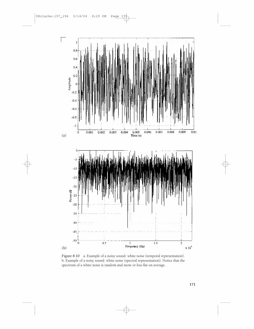
For the sound characterization to be complete, the category of noisy sounds hasto be considered. By definition, these have a random temporal representation (suchas the whispered sound between 2.2 and 3.2 seconds in Figure 8.3). Few instru-mental sounds are completely noisy, but most of them include a certain amount ofnoise (the player’s breath in the case of wind instruments, impact noise for percus-sion, and so on), and as we shall later see, this noisy part is nearly always very im-portant for the perception of timbre. The sounds of wind and surf, replicated byelectronic noise generators, are by contrast completely noisy. Such sounds are com-posed of a random mix of all possible frequencies, and their spectral representationis the statistical average of the spectral components. For example, white noise has arandom waveform (Figure 8.10a). Although it has a spectrum that is theoreticallyflat, with all frequencies appearing at the same level, in practice the spectrum re-vealed by Fourier analysis is far from being perfectly flat (Figure 8.10b), and exhibitsvariations that are due to the lack of averaging of the random fluctuations in level ofthe different frequencies. These fluctuations can be reduced by taking the average ofseveral spectra computed on successive time-limited samples of the noisy sound.

Now that the basic characteristics of sounds have been described, it is impor-tant to mention one major aspect of “natural” sound signals: their characteristics(frequency, amplitude, waveform, inharmonicity, or noise content) always vary overtime. Sounds with perfectly stable characteristics (such as the sinusoids in Figure8.6, or the stable low-frequency sound in Die Roboten, between 2 and 3 seconds inFigure 8.2) sound “unnatural” or “synthetic..” These time-varying characteristics arecalled modulations and can take various forms. Amplitude modulations range fromuncontrolled random fluctuations, such as in the flute note in Figure 8.4, to thetremolo on the low sustained note in Die Roboten (between 1.5 and 2 seconds in Fig-ure 8.2); frequency modulations can include vibrato (the undulating horizontal linesproduced by the piccolo during the first 1.5 second of Figure 8.1b) or pitch glides(the upward sweeping “chirp” sound in Die Roboten between 3.8 and 4.5 seconds,Figure 8.2). Apart from their impact on the character of individual sounds, the pres-ence and synchronization of modulations are very important for the perception offused sounds, and will be discussed in the final section of this chapter.

This means that there is a significant element of approximation or idealizationin all but the simplest representations of sound which we have been discussing.Most obviously, spectral representations (Fourier or otherwise) relate amplitude andfrequency: they represent values averaged over a discrete temporal “window” or“frame,” and therefore tell us nothing about changes in the sound during that periodof time. (One could represent the changes by showing a series of spectral represen-tations one after another, in the manner of an animation, but even then each frame


08clarke.157_196 3/14/04 8:29 PM Page 167


Figure 8.8 a.1. Sawtooth waveform. a.2. Spectrum(Fourier series) of a sawtooth waveform. b.1. Square wave-form. b.2. Spectrum (Fourier series) of a square waveform.c. Spectrum (Fourier series) of a clarinet waveform.

(a.1)

(a.2)

would represent the average over a given time span.) There is also a similar point inrelation to periodicity. While from a mathematical point of view a periodic signal re-produces exactly the same cycle indefinitely, in the real world any sound has a be-ginning and an end: for this reason alone, musical sounds are not mathematicallyperiodic. Moreover, they nearly always show slight differences from one period tothe next (as can be seen from the waveform of the clarinet sound in Figure 8.5). Inpractice, a sound is perceived as having a definite pitch as soon as there is a suffi-cient degree of periodicity, not when it is mathematically periodic, and we thereforeneed an analytical tool that will identify degrees of periodicity on a local basis, show-

08clarke.157_196 3/14/04 8:29 PM Page 168

(b.1)

(b.2)

(c)

169

08clarke.157_196 3/14/04 8:29 PM Page 169

Figure 8.9 a. Inharmonicity: spectrum of a bell sound. The series of vertical thin linesrepresent theoretical locations of a harmonic series of fundamental frequency 103 Hz.b. Inharmonicity: spectrum of a tympani sound. The series of vertical thin lines representtheoretical locations of a harmonic series of fundamental frequency 66 Hz. c. Inharmoni-city: spectrum of a piano sound. The series of vertical dashed lines represents theoreticallocations of a harmonic series of a fundamental frequency of 831 Hz.

ED: had to runcaption full width

to fit all on onepage. –Comp.

(a)

(b)

(c)

170

08clarke.157_196 3/14/04 8:29 PM Page 170

Figure 8.10 a. Example of a noisy sound: white noise (temporal representation).b. Example of a noisy sound: white noise (spectral representation). Notice that thespectrum of a white noise is random and more or less flat on average.

(a)

(b)

171

08clarke.157_196 3/14/04 8:29 PM Page 171

ing how the spectrum changes over time. This is exactly what the spectrogram does,as illustrated in the introduction of this chapter—and this, again, is something towhich we will return.

Acoustical Analysis of Sounds

A waveform display allows a user to analyze a sound quite intuitively by simplylooking at a temporal representation of a sound. The representation can be createdat different time scales, from the “microscopic” or short-term scale, to the “macro-scopic” or long-term scale. A “microscopic” time scale, which in practice is usuallyon the order of a few periods, preserves the waveform shape, and allows a qualita-tive evaluation of the presence or absence of noise and its level, as well as the pres-ence of strong, high-order harmonic components. Figures 8.5a, 8.6a, 8.7a, 8.8a.1,and 8.8b.1 are temporal representations of signals at a “microscopic” time scale: thisalso allows one to evaluate precisely the synchronization between acoustic events.By contrast, a “macroscopic” time scale makes visible long-term tendencies such asthe global evolution of the sound level, amplitude changes in the course of a melodicline, or the way notes follow one another; an example is Figure 8.4 in which the tem-poral envelope of a flute sound can be discerned.

Sound signals are usually displayed on computer screens using sound editorprograms; some examples are ProTools, AudioSculpt, Peak, SpectroGramViewer, andAudacity. However there is a problem when the number of samples to be representedon the screen becomes larger than the number of available pixels: as sounds are usu-ally sampled at 44,100 Hz (the compact disc standard), and as the highest numberof pixels on each line of current screens is usually less than 2000, a complete displayis possible only for durations shorter than 50 milliseconds (msec). Beyond that, sev-eral sample values have to be averaged into one pixel value (in other words, the sig-nal has to be smoothed), and this prevents precise investigation of long-term soundcharacteristics, limiting the direct use of “macroscopic” sound signal displays to theanalysis of global temporal evolutions. Even in the case of these global evolutions,though, there is a perceptually more meaningful means of analysis: temporal envelopeestimation.

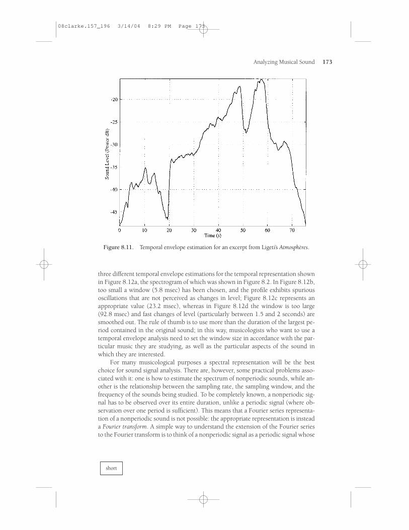
As an example, Figure 8.11 displays the dynamic evolution of an excerpt fromLigeti’s orchestral piece Atmosphères, starting with a slow crescendo/decrescendo overthe first 20 seconds, followed by a fast crescendo to a median level, and a slow cres-cendo for the next 30 seconds, and so on. Such a temporal envelope, which is cal-culated automatically by most sound editing programs, is again based on a series oftemporal windows or frames, the duration of which is normally between 10 and 200msec, with the window sliding along the time axis to provide an estimate of the tem-poral envelope at set intervals. The only setting that you need to adjust in order toget a temporal envelope is the size of the window. The chosen size will inevitably bea compromise: it has to be large enough to smooth over the fine-grained oscillationsof the signal, but at the same time small enough to preserve the shape of the attack,or of the other transient parts of the sound. The problem can be seen by comparing


short

08clarke.157_196 3/14/04 8:29 PM Page 172

three different temporal envelope estimations for the temporal representation shownin Figure 8.12a, the spectrogram of which was shown in Figure 8.2. In Figure 8.12b,too small a window (5.8 msec) has been chosen, and the profile exhibits spuriousoscillations that are not perceived as changes in level; Figure 8.12c represents an appropriate value (23.2 msec), whereas in Figure 8.12d the window is too large(92.8 msec) and fast changes of level (particularly between 1.5 and 2 seconds) aresmoothed out. The rule of thumb is to use more than the duration of the largest pe-riod contained in the original sound; in this way, musicologists who want to use atemporal envelope analysis need to set the window size in accordance with the par-ticular music they are studying, as well as the particular aspects of the sound inwhich they are interested.

For many musicological purposes a spectral representation will be the bestchoice for sound signal analysis. There are, however, some practical problems asso-ciated with it: one is how to estimate the spectrum of nonperiodic sounds, while an-other is the relationship between the sampling rate, the sampling window, and thefrequency of the sounds being studied. To be completely known, a nonperiodic sig-nal has to be observed over its entire duration, unlike a periodic signal (where ob-servation over one period is sufficient). This means that a Fourier series representa-tion of a nonperiodic sound is not possible: the appropriate representation is insteada Fourier transform. A simple way to understand the extension of the Fourier seriesto the Fourier transform is to think of a nonperiodic signal as a periodic signal whose


Figure 8.11. Temporal envelope estimation for an excerpt from Ligeti’s Atmosphères.

short

08clarke.157_196 3/14/04 8:29 PM Page 173

period is infinite. An example of a nonperiodic signal and its Fourier transform isgiven in Figure 8.13. The sound signal is a damped sinusoid, that is a sinusoidwhose amplitude decreases over time. The treatment of this kind of signal is signif-icant, since many percussion instruments (including bells, timpani, pianos, and xy-lophones) produce a superposition of damped sinusoids.

The Fourier transform (Figure 8.13b) exhibits a maximum close to the oscillat-ing frequency, but there is some power at other frequencies, particularly those closeto the central frequency. The sharpness of the maximum, sometimes called a for-


Figure 8.12 a. Temporal representation of the firstthree seconds of Die Roboten by Kraftwerk. b. Temporalenvelope estimation of the sound signal displayed inFigure 8.12a. using a window size of 5.8 msec. c. Tem-poral envelope estimation of the sound signal displayedin (a). using a window size of 23.2 msec. d. Temporalenvelope estimation of the sound signal displayed inFigure 12.a. using a window size of 92.8 msec.

(a)

(b)

08clarke.157_196 3/14/04 8:29 PM Page 174

mant, varies in inverse proportion to the degree of damping. The damping makes theoscillating sinusoid nonperiodic and spreads its power out to other frequencies; thespectrum is therefore no longer a peak (as it is for a pure sinusoid) but a smoothedcurve, whose bandwidth (the width of the curve) increases with the damping value.

As in the case of temporal envelope estimation, choosing the right duration asthe basis for calculating the Fourier transform is a compromise: the duration needsto be small enough to maintain sufficient resolution between closely adjacent sinu-soids, and yet not so large as to average out all of the temporal evolution of thesound’s spectral characteristics. A good compromise is usually a duration of four tofive times the period of the lowest frequency difference between the sinusoidal com-ponents of the sound. Figure 8.14 revisits the spectral analysis of the A major chord,made up of three sinusoidal sounds, that was shown in Figure 8.7: since the fre-quencies are 440, 550, and 660 Hz, the lowest frequency difference is 110 Hz,which (at a 44,100 Hz sampling rate) corresponds to approximately 400 samples.Figure 8.14 shows that a window size of 2,048 samples i.e., approximately 5 times400 samples) successfully separates out the three components.


(d)

(c)

08clarke.157_196 3/14/04 8:29 PM Page 175


Figure 8.13 a. Nonperiodic signal: a damped sinusoid (frequency = 440 Hz). b. Non-periodic signal: spectrum of a damped sinusoid (frequency = 440 Hz). Notice the contin-uous aspect of the spectrum.

(a)

(b)

08clarke.157_196 3/14/04 8:29 PM Page 176

We are now ready to come full circle, establishing the link between all the con-cepts developed in this section and the spectrographic representation at the very be-ginning of the chapter. A spectrum, resulting from a Fourier transform performedover a finite duration, provides useful information about a sound signal only whenthe sound is known to be stable in time. However, as already mentioned, the char-acteristics of natural sounds always vary in time. A spectrum taken from a windowlocated at the beginning of a sound (Figure 8.15a) is usually different from a spec-trum taken from a window located in the middle of the sound (Figure 8.15b). Inorder to describe the temporal variations of the spectral properties of a sound, asimple idea is to compute a series of evenly spaced local spectra. This is achieved bycomputing a Fourier transform for each of a series of sliding windows taken fromthe signal. The time-step increment of the sliding window is usually a proportion ofthe window size, and a time-shift of an eighth of the window size or less ensures per-fect tracking of the temporal evolution. Each Fourier transform represents an esti-mate of the spectral content of the signal at the time on which the window is cen-tered, and a simple and efficient way to display this series of spectra is to create atime/ frequency representation, with the darkness of the trace representing the am-plitude of each frequency (Figure 8.16). This representation, which we have alreadyencountered, is called a spectrogram (or sometimes a sonogram).

In summary, we have seen two different kinds of two-dimensional representa-tion of sound, and a three dimensional representation. The two-dimensional repre-


Figure 8.14. Time-limited Fourier analysis: spectrum of the major chord fromFigure 8.7 estimated with a window size of 2,048 samples.

08clarke.157_196 3/14/04 8:29 PM Page 177


Figure 8.15 a. Spectrum of a bass clarinet tone during the attack (window centered on0.12 second, window size of 4,096 samples). b. Spectrum of a bass clarinet tone duringthe sustained part (window centered on 1 second, window size of 4,096 samples).

(a)

(b)

08clarke.157_196 3/14/04 8:29 PM Page 178

sentations are temporal representations (amplitude against time), and spectral rep-resentations (amplitude against frequency); the three-dimensional representation—the spectrogram—shows frequency against time on the two axes, and intensityagainst time in the blackness of the trace.

Analytical Applications

The most sustained example of applying acoustical principles to musical analysis,and one which makes considerable use of spectrograms, is Robert Cogan’s book NewImages of Musical Sound (Cogan 1984). The central part of the book consists of a dis-cussion and analysis of 17 “spectrum photos” (the equivalent of spectrograms) ofmusic from a wide variety of traditions, including Gregorian chant, jazz, a move-ment of a Beethoven piano sonata, electroacoustic music, and Tibetan tantric chant;the examples range from half a minute to over 11 minutes in duration, with the ma-jority around two to four minutes long. The spectrum photos show duration on thehorizontal axis and frequency on the vertical axis, with intensity represented as thebrightness of the trace (in other words, while intensity is represented by blacknessagainst a white background in the spectrograms presented in this chapter, it isshown as whiteness against a black background in Cogan’s photos). The spectrumphotos were created using analog signal analysis equipment, with a camera used totake photographs of the cathode ray tube for successive sections of music; these were


Figure 8.16. Spectrogram of a bass clarinet sound (window size of 4,096 samples,time-step increment of 512 samples).

08clarke.157_196 3/14/04 8:29 PM Page 179

then literally pasted together to create the resulting composite photos that appear inthe book. Digital technology has made it possible to produce more flexible and finelygraded representations of this kind far more easily, as the figures in this chapter dem-onstrate.

Cogan uses the spectrum photos to analyze and demonstrate a variety of differ-ent features of the music, the diversity of which is intended to show how many dif-ferent features can be addressed through these means. His discussion of Billie Holi-day’s recording of “Strange Fruit,” for example, focuses on the ways in which Holidayuses continuous pitch changes and the timbral effects of different vowel sounds toarticulate semantic relationships in the text, and to expose its savage ironies: “Notebending is a motif that recurs with ever-increasing intensity. ‘The gallant South’ isimmediately echoed with growing irony at ‘sweet and fresh,’ again bending to thevoice’s lowest depth. Then a string of increasingly bent phrases. . . . leads with gath-ering intensity to the explicit recall of the first stanza . . . ” (Cogan 1984: 35)

By comparison, the discussion of Elliott Carter’s Etude III for Wind Quartet fo-cuses on the timbral changes that result both from instrumental entries and exits,and from continuous dynamic changes, rhythmic augmentation, and diminution.This analysis is unusual in using spectral representations (rather than temporal rep-resentations) to give more detail about the relative balance of different spectral com-ponents in the sound than is possible in the spectrograms used elsewhere in thebook: because time is eliminated from the representation, Cogan presents a se-quence of 18 spectral “snapshots” to demonstrate how the timbre evolves over thepiece. Without getting involved in the detail of Cogan’s analysis, a sense of what heclaims such an analysis can achieve can be gathered from the following (Cogan1984: 71–72):

Spectrum analysis provides a tool whereby the important similarity of thesepassages—the initial one characterized by instrumental change and rhythmicdiminution, the climactic one by dynamic change and rhythmic augmenta-tion—can be discovered and shown. Remove the spectral features and themost critical formal links of the entire etude . . . disappear. Without spectralunderstanding, the link between the successive transformations—instrumen-tal, rhythmic, and dynamic . . . would evaporate. . . . We noted at the begin-ning of this commentary that, in the light of earlier analytic methods, thisetude could emerge only as incomprehensible, static, or both. It now, how-ever, reveals itself to be a set of succinct, precise spectral formations whoseroles and relationships, whether of identity or opposition, are clear at everyinstant.

Two further examples of the way in which spectral analysis can be used for mu-sicological purposes are provided by Peter Johnson’s (1999) discussion of two per-formances of the aria “Erbarme Dich” from Bach’s St. Matthew Passion, and DavidBrackett’s (2000) analysis of a track by Elvis Costello. The subject of Johnson’s paperis a wide-ranging discussion of the relationship between performance and listening,with Bach’s aria as a focal example viewed from aesthetic and more concretely ana-lytical perspectives. Central to Johnson’s argument is his insistence that the impactof the sound of a performance on listeners’ experience is consistently underestimated


08clarke.157_196 3/14/04 8:29 PM Page 180

by commentators and analysts, and an important part of the paper is thus devotedto a detailed consideration of the acoustical characteristics of two performances ofthe aria. Johnson focuses primarily on differences in the frequency domain, high-lighting distinctions in the use of vibrato, timbre, and intonation in the first eightbars of the aria as taken from recordings directed by John Eliot Gardiner and KarlRichter. On the basis of both spectral and temporal representations of the soundcharacteristics of the first few bars of the instrumental opening of the aria, obtainedusing the signal processing and plotting software in the Matlab program, Johnsondemonstrates how Gardiner’s recording features a more transparent timbre, muchless vibrato in the solo violin part, and a more fluctuating amplitude profile, with aconsistent tendency for the amplitude to drop away at group and phrase endings;Richter’s recording, by contrast, demonstrates a more constant vibrato and ampli-tude level, a thicker timbre, and the use of expressive intonation (a flattening of themediant note).

Johnson acknowledges that

much of what is shown by spectrographic analysis is little more than a visualanalogue of what we have already recognized and perceived through listening.Nonetheless, acoustic analysis reinforces the experiential claims of the listen-ing musician, namely that (1) performance can significantly determine theproperties of the experience itself, and (2) the listening experience is notwholly private: hearing is not entirely “subjective” in the sense of a strictly un-verifiable or purely solipsistic mode of perception. . . . Finally, acoustic analy-sis is a powerful medium for the education of the ear and as a diagnostic toolfor the conscientious performer, the didactic possibilities of which have barelybegun to be exploited. ( Johnson 1999: 83–84)

In fact Johnson uses the acoustic characteristics of the two recordings to argue thatthe two interpretations offer distinctly different musical and theological perspec-tives. Richter’s recording, he claims, conveys a sense of reverence and authority (inrelation both to Bach and the biblical narrative) in its even lines, thick textures, con-stant amplitude, tempo and vibrato, and solemnly “depressed” expressive intona-tion. Gardiner’s, by contrast, is more enigmatic, using a faster and more flexibletempo and a more transparent sound to conjoin the secular connotations of dancewith the seriousness of the biblical text; Johnson describes it as a “rediscovery inlater 20th century Bach performance practice of the physical, the kinesthetic, not(here) as licentiousness but as a medium through which even a Passion can find new(or old) meanings.” ( Johnson 1999: 99)

Brackett’s (2000) use of spectrum photos is more cursory and restricted, butworth considering because of the comparative rarity of this approach in the study ofpopular music—perhaps surprisingly, given that it is a non-score-based tradition inwhich acoustic characteristics (such as timbre, texture and space) are acknowledgedto be of particular importance. Brackett’s aim in his chapter on Elvis Costello’s song“Pills and Soap” is to demonstrate various ways in which Costello maintains an elu-sive relationship with different musical traditions—particularly in his negotiationswith art music. Brackett uses spectrum photos similar to Cogan’s to make pointsabout both the overall timbral shape of “Pills and Soap,” and more detailed aspects


08clarke.157_196 3/14/04 8:29 PM Page 181

of word setting. An example of the latter is Brackett’s demonstration (p. 187) that suc-cessive repetitions of the word “needle” in the song become increasingly timbrallybright and accented, as a way of drawing attention to the word and its narrative/semantic function. At a “middleground” level, he points out that vocal timbre (aswell as pitch height) is used to give a sense of teleology to each verse, pushing thesong forward. Finally (and this is where the connection with art music becomesmore explicit), Brackett uses spectral information to support his claim that the songrepresents a particular kind of skirmish with Western “art” music. He shows how anincreasingly oppositional relationship between high- and low-frequency timbralcomponents characterizes the large-scale shape of the song, and argues that this

is much more typical of pieces of Western art music than it is of almost anyother form of music in the world, be it popular, “traditional,” or non-Western“art” music. Examination of the photos in Robert Cogan’s New Images of Musi-cal Sound reveals a greater similarity between the spectrum photo of “Pills and Soap” and the photos of a Gregorian chant, a Beethoven piano sonata, the “Confutatis” from Mozart’s Requiem, Debussy’s “Nuages,” and Varèse’sHyperprism, than between “Pills and Soap” and the Tibetan Tantric chant orBalinese shadow-play music. For that matter, the photo of “Pills and Soap”more closely resembles these pieces of art music than it does the photo for“Hey Good Lookin,” the photo of which may reveal timbral contrast on a local level without that contrast contributing to a larger sense of teleologicalform. (Brackett 2000: 195)

Whether the argument that Brackett advances here stands up to scrutiny or not(there might be all kinds of reasons why “Pills and Soap” doesn’t have a spectralshape that looks anything like Tibetan chant, Balinese shadow-play music, or an-other arbitrarily chosen popular song), the point that it makes is that the empiricalevidence provided by spectral and temporal representations can furnish an impor-tant tool in a musicological enterprise—and that is what this chapter is intended todemonstrate.

The examples presented here, however, also illustrate some of the problems andpitfalls of using such information; it is very hard to find representational methodsand analytical approaches that successfully reconcile detailed investigation withsome sense of overall shape. Johnson’s analysis, in focusing on the details of vibrato,timing, and intonation, doesn’t go beyond bar 8 of the Bach aria; by contrast, Brack-ett’s analysis of Costello, and many of Cogan’s analyses, present spectrum photos atsuch a global level and with such inadequate resolution that some of the features anddistinctions they discuss are all but invisible—and have to be taken on trust to moreor less the same degree as if the authors were simply to tell the reader that the timbregets brighter, or that there’s a tiny articulation between phrases, or that there is anincreasing accent on a word. In other words, there is a question about whether allthe visual apparatus can really convince a reader of very much at all.

In part this is a purely technological matter, and the technology has certainlyimproved dramatically since the time of Cogan’s book. But as shown by the muchmore sophisticated representations that Johnson uses, and as argued in this chapter,the problem is by no means solved by technological progress: there is still a real


08clarke.157_196 3/14/04 8:29 PM Page 182

problem in extracting the salient features from a data representation that contains apotentially overwhelming amount of information, only a tiny fraction of which maybe relevant at any moment. The problem is testimony to the extraordinary analyti-cal powers of the human auditory system: in the mass of detail that is presented ina ‘“close-up” view of the sound, the auditory system finds structure and distinctive-ness. Some of the principles that account for this human capacity, and the ways inwhich they may contribute to musicological considerations, are the subject of thefinal section of this chapter.

Perceptual Analysis of Sounds

Music presents a challenge to the human auditory system, because it often containsseveral sources of sound (instruments, voices, electronics) whose behavior is coor-dinated in time. In order to make sense of this kind of musical material, the charac-teristics of the individual sounds, of concurrent combinations of them, and of se-quences of them, must be identified by the auditory system. But to do this, the brainhas to “decide” which bits of sound belong together, and which bits do not. As wewill see, the grouping of sounds into perceptual units (events, streams, and textures)determines the perceived properties or attributes of these units. Thus, in consider-ing the perceptual impact of the sounds represented in a score or a spectrogram, itis necessary to keep in mind a certain number of basic principles of perceptual pro-cessing.

Music played by several instruments presents a complex sound field to thehuman auditory system. The vibrations created by each instrument are propagatedthrough the air to the listeners’ ears, and combine with those of the other instru-ments as well as with the echoes and reverberations that result from reflections offwalls, ceiling, furniture, and so on. What arrives at the ears is a very complex wave-form indeed. To make matters worse, this composite signal is initially analyzed as awhole. The vibrations transmitted through the ear canal to the eardrum and thenthrough the ossicles of the middle ear are finally processed biomechanically in theinner ear (the cochlea), such that different frequency regions of the incoming signalstimulate different sets of auditory nerve fibers. This is the aural equivalent of thespectral analysis described in the first main section of this chapter; one might con-sider the activity in the auditory nerve fibers over time as a kind of neural spectro-gram. So if several instruments have closely related frequencies of vibration in theirwaveforms, they will collectively stimulate the same fibers: that is, they will be mixedtogether in the sequence of neural spikes that travel along that fiber to the brain. Aswe shall see, this would be the case for the different instruments playing the Boléromelody in parallel in a close approximation to a harmonic series.

It should be noted, however, that the different frequencies are still representedin the time intervals between successive nerve spikes, since the time structure of thespike train is closely related to the acoustic waveform. Furthermore, a sound from asingle musical instrument is composed of several different frequencies (see the bassclarinet example in Figure 8.16) and thus stimulates many different sets of fibers;that is, it is analyzed into separate components distributed across the array of audi-


08clarke.157_196 3/14/04 8:29 PM Page 183

tory nerve fibers. The problem that this presents to the brain is to aggregate the sep-arate bits that come from the same source, and to segregate the information thatcomes from distinct sources. Furthermore, the sequence of events coming from thesame sound source must be linked together over time, in order to follow a melodyplayed by a given instrument. Let us consider a few examples of the kinds of prob-lem that this poses.

In some polyphonic music (such as Bach’s orchestral suites or Ligeti’s WindQuintet), the intention of the composer is to create counterpoint, the success ofwhich clearly depends on achieving segregation of the different instruments (Wrightand Bregman 1987): what must be done to ensure that the instruments don’t fusetogether? In other polyphonic music, however (Ravel’s Boléro, Ligeti’s Atmosphères),the composer may seek a blending of different instruments and this would dependon achieving fusion or textural integration of the instruments: what must the musi-cians do to maximize the fusion and how can this be evaluated objectively? Finally,in some instrumental music an impression of two or more “voices” can be createdfrom a monophonic source (such as in Telemann’s recorder music or Bach’s cellosuites), or a single melodic line may be composed across several timbrally distinctinstruments (as in Webern’s Six Pieces for Large Orchestra, op. 6): what determinesmelodic continuity over time, and how might the integration or fragmentation bepredicted from the score or for a given performance? For all these questions, themost important issue is how the perceptual result can be characterized from repre-sentations of the music (scores for notated music, acoustic representations for re-corded or synthesized music). Obviously one can simply listen and use an aurallybased analytical approach, but this restricts the account to the analyst’s own (per-haps idiosyncratic) perceptions; if the aim is to provide a more generalized inter-pretation, the solution is to use basic principles of auditory perception as tools forunderstanding the musical process.

Grouping processes determine the perception of unified musical events (notes oraggregates of notes forming a vertical sonority), of coherent streams of events (hav-ing the connectedness necessary to perceive melody and rhythm), and of more orless dense regions of events that give rise to a homogeneous texture. Perceptual fu-sion is a grouping of concurrent acoustic components into a single auditory event (aperceptual unit having a beginning and an end); the perception of musical attributessuch as pitch, timbre, loudness, and spatial position depends on which acousticcomponents are grouped together. Auditory stream integration is a grouping of se-quences of events into a coherent, connected form, and determines what is heard asmelody and rhythm. Texture is a more difficult notion to define, and has been theobject of very little perceptual research, but intuitively the perception of a homoge-nous musical texture requires a grouping of many events across pitch, timbre, andtime into a kind of unitary structure, the textural quality of which depends on therelations among the events that are grouped together (certain works by Ligeti,Xenakis, and Penderecki come to mind, as do any number of electroacoustic works).Note that the main notion behind the word “grouping” is a kind of perceptual con-nectedness or association, called “binding” by neuroscientists. It seems clear thatmany levels of grouping can operate simultaneously, and that what is perceived de-pends to some extent on the kind of structure upon which a listener focuses. Since


08clarke.157_196 3/14/04 8:29 PM Page 184

a large amount of scientific research has been conducted on concurrent and se-quential sound organization processes, we will consider these in more detail, beforemoving on to discuss the perception of the musical properties (spatial location,loudness, pitch, timbre) that emerge from the auditory images formed by the pri-mary grouping process.

There are two main factors that determine the perceptual fusion of acousticcomponents into unified auditory events, or their segregation into separate events:onset synchrony and harmonicity. A number of other factors were originally thoughtby perception researchers to be involved in grouping, but are probably more impli-cated either in increasing the perceptual salience of an event (vibrato and tremolo),or in allowing a listener to focus on a given sound source in the presence of severalothers (spatial position; for reviews see McAdams 1984, Bregman 1990, 1993, Dar-win and Carlyon 1995, Deutsch 1999). We will focus here on the grouping factors.

Acoustic components that start at the same time are unlikely to arise from dif-ferent sound sources and so tend to be grouped together into a single event. Onsetasynchronies between components on the order of as little as 30 msec are sufficientto give the impression of two sources and to allow listeners in some cases to identifythe sounds as separate; to get a perspective on the accuracy necessary to producesynchrony within this very small time window, one might note that skilled profes-sional musicians playing in trios (strings, winds, or recorders) have asynchronies inthe range of 30 to 50 msec, giving a sense of playing together while allowing per-ceptual segregation of the instruments (Rasch 1988). If musicians play in perfectsynchrony, by contrast, there is a greater tendency for their sounds to fuse togetherand for the identity of each instrument or voice to be lost. These phenomena canalso be manipulated compositionally: Huron (1993) has shown by statistical analy-ses that the voice asynchronies used by Bach in his two-part inventions were greaterthan those used in his work as a whole, suggesting an intention on the part of thecomposer to maximize the separation of the voices in these works. If, on the otherhand, voices in a polyphony are synchronous, what may result is a global timbre thatcomes from the fusion of the composite—though considerable precision is neededto achieve such a result.

The other main grouping principle is that sound components tend to be per-ceived as a single entity when they are related by a common fundamental period.This is particularly the case if, when the fundamental period changes, all of the com-ponents change in similar fashion, as would be the case in playing vibrato, or in asingle instrument playing a legato melody. Forced vibrating systems such as blownair columns (wind instruments) and bowed strings create nearly perfect harmonicsounds, with a strongly fused quality and an unambiguous pitch—in contrast to theseveral audible pitches of some inharmonic, free-vibrating systems such as a struckgong or church bell. This harmonicity-based fusion principle has again been usedintuitively by composers of polyphonic music: a statistical analysis of Bach’s key-board music by Huron (1991) showed that the composer avoided harmonic inter-vals in proportion to the degree to which they promote tonal fusion, thus helping toensure voice independence.

An important perceptual principle is demonstrated through such fusion: ifsounds are grouped together, the perceptual attributes that arise—such as a new


08clarke.157_196 3/14/04 8:29 PM Page 185

composite timbre—may be different from those of the individual constituent sounds,and may be difficult to imagine merely from looking at the score or even at a spec-trogram. The principle that the perceived qualities of simultaneities depend ongrouping led Wright and Bregman (1987) to examine the role of nonsimultaneousvoice entries in the control of musical dissonance: they argued that the dissonant ef-fect of an interval such as a major seventh is much reduced if the voices composingthe interval do not enter synchronously, and similar results also apply to fusionbased on harmonicity (see McAdams 1999). All this demonstrates the need to con-sider issues of sonority in the perceptual analysis of pitch structures.

As a concrete example, Ravel’s Boléro arguably represents an example of in-tended fusion. Up to bar 148, the main melody is played in succession by differentinstrumental soloists. But at this point it is played simultaneously by five voices onthree types of instrument: French horn, celesta, and piccolos (Figure 8.1b); the basicmelody is played by the French horn, and is transposed to the octave, 12th, doubleoctave, and double octave plus a major third for the celesta (LH), piccolo (2), celesta(RH), and piccolo (1), respectively. Note that this forms a harmonic series and thatthese harmonic intervals are maintained since the transpositions are exact (so thatthe fundamental, octave, and double octave melodies are played in C major, the 12thmelody in G major, and the double octave plus a third melody in E major). Ravel thusrespects the harmonicity principle to the letter, and since all the melodies are alsopresented in strict synchrony, the resulting fusion—with the individual instrumentidentities subsumed into a single new composite timbre—depends only on accuratetuning and timing being maintained by the performers. This procedure is repeatedby Ravel for various other instrumental combinations in the course of the piece, theconsequent timbral evolution contributing to the global crescendo of the piece.

An inverse example can be found in the mixed instrumental and electroacousticwork Archipelago by Roger Reynolds, for ensemble and four-channel computer-generated tape. In the tape part, recordings of the musical materials used elsewherein the work by different instruments were analyzed by computer and resynthesizedwith modifications. In particular, the even and odd harmonics were either processedtogether as in the original sound, giving a temporally extended resynthesis of thesame instrument timbre, or processed separately with independent vibratos and spa-tial trajectories, resulting in a perceptual fission into two new sounds. Selecting onlythe odd harmonics of an instrument sound leaves the pitch the same, but makes thetimbre more “hollow” sounding, moving in the direction of a clarinet sound (whichhas weak even-numbered harmonics in the lower part of its frequency spectrum);selecting only the even harmonics produces an octave jump in pitch, since a seriesof even harmonics is the same as a harmonic series an octave higher. The perceptualresult is therefore two new sounds with pitches an octave apart and timbres that arealso different compared to the original sound. An example from Archipelago is thesplit of an oboe sound (Figure 8.17), which resulted in a clarinetlike sound at theoriginal pitch and a sopranolike sound an octave higher. When the vibrato patternswere made coherent again, the sound fused back into the original oboe.

Sequential sound organization concerns the integration of successive eventsinto auditory streams and the segregation of streams that appear to come from dif-ferent sources. In real-world settings, a stream generally constitutes a series of events


08clarke.157_196 3/14/04 8:29 PM Page 186

emitted over time by a single source. As we will see, however, there are limits to whata listener can hear as an auditory stream, which does not always correspond to whatreal physical sources can actually do. So we can say that an auditory stream is a co-herent “mental” representation of a succession of events. The main principle that af-fects this mental coherence is a trade-off between the temporal proximity of succes-sive sound events and their relative similarity: the brain seems to prefer to connecta succession of sounds of similar quality which together create a perceptual conti-nuity. Continuity, however, is relative since a given difference between successiveevents may be perceived as continuous at slow tempi, but will be split into differentstreams at fast tempi. The main parameters affecting continuity include spectrotem-poral properties, sound level, and spatial position; continuous variation in all ofthese parameters gives a single stream, whereas rapid variation (particularly in allthree together, as would often be the case for two independent sound sources play-ing at the same time) can induce the fission of a physical sequence of notes into twostreams, one corresponding to the sequence emitted by each individual instrument.

In order to illustrate the basic principles, let us examine spectrotemporal conti-nuity, which is affected by pitch and timbre change between successive notes.Melodies played by a single instrument with steps and small skips tend to be heardas unified, with easily detectable pitch and rhythmic intervals, while rapid jumps


Figure 8.17. Splitting of an oboe sound in the Roger Reynolds’s Archipelago. At around 3 seconds the odd-numbered harmonics start to have an independentvibrato which grows and then decays in strength. A similar pattern occurs on theeven-numbered harmonics from about 5 seconds. Finally, each group swells invibrato, but with independent vibration patterns at around 9 seconds.

08clarke.157_196 3/14/04 8:29 PM Page 187

across registers or between instruments may give rise to the perception of two ormore melodies being played simultaneously, as illustrated in Figure 8.18 (an excerptfrom a recorder piece by Telemann). In this case the perceived “melody” (i.e., thespecific pattern of pitch and rhythmic intervals) corresponds to the relationshipsamong the notes that have been grouped into a single stream or into multiplestreams. Over the first six seconds of the excerpt shown, a listener will hear (and thespectrogram shows) a relatively slow ascending melody, a static pedal note, and a se-quence of more rapid three note descending motifs. Because listeners often havegreat difficulty perceiving relations across streams, such as rhythmic intervals andeven relative temporal order of events, there can be some surprising rhythmic resultsfrom apparently simple materials. The example in Figure 8.19 illustrates how twointerleaved, isochronous rhythms played by separate xylophone players can pro-duce a complex rhythmic pattern (note the irregular spacing of the sound events inthe 250 to 1,000 Hz range in the spectrogram) due to the way the notes from thetwo players are combined perceptually into a single stream with unpredictable dis-continuities in the melodic contour.

Once the acoustic waveform has been analyzed into separate source-relatedevents, the auditory features of the events can be extracted. These musical qualitiesdepend on various acoustic properties of the events, of which the most importantare spatial location, loudness, pitch, and timbre. Each of these will be consideredseparately.


Figure 8.18. Spectrogram of an excerpt of a recorder piece by Telemann. The funda-mental frequencies of the recorder notes lie in the range 400 to 1,500 Hz.

08clarke.157_196 3/14/04 8:29 PM Page 188

The spatial location of an event depends on several kinds of cues in the sound.In the first place, since we have two ears that are separated in space, the sound thatarrives at the two ear drums depends on the position of the sound source relative tothe listener’s head, and is different for each ear: a sound coming from one side is bothmore intense and arrives earlier at the closer ear. Also the convoluted, irregularshape of the outer part of the ear (the pinna) creates position-dependent modifica-tions of the sound entering the ear canal, and these are interpreted by the brain ascues for localization. Second, and more difficult to research, are the cues that allowus to infer the distance of the source (Grantham 1995). There are several possibleacoustic cues for distance: one is the relative level, since level decreases as a functionof distance, while another is the relative amount of reverberated sound in the envi-ronment as compared with the direct sound from the source (the ratio of reverber-ated to direct sound increases with distance). Finally, since higher frequencies aremore easily absorbed and/or dispersed in the atmosphere than are lower frequen-cies, the spectral shape of the received signal can also contribute to the impressionof distance. Such binaural, pinna, and distance cues are useful in virtual reality dis-plays and in creating spatial effects in electroacoustic music.

For simple sounds loudness corresponds fairly directly to sound level; but forcomplex sounds, the global loudness results from a kind of summation of poweracross the whole frequency range. It is as if the brain adds together the activity in allof the auditory nerve fibers that are being stimulated by a musical sound to calcu-


Figure 8.19. Spectrogram of a rhythm played by separate players on an Africanxylophone.

08clarke.157_196 3/14/04 8:29 PM Page 189

late the total loudness. When several sounds are present at the same time and theirfrequency spectra overlap, a louder sound can cover up a softer sound either par-tially, making it even softer, or totally, making it inaudible: this process is calledmasking, and seems to be related to the neural activity of one sound swamping thatof another. Masking may be partially responsible for the difficulty in hearing outinner voices when listening to polyphonies with three or more voices. Again, loud-ness is affected by duration: a very short staccato note (say around 50 msec) with thesame physical intensity as a longer note (say around 500 msec) will sound softer.This seems to be because loudness accumulates over time, and the accumulationprocess takes time: for a long steady note, the perceived loudness levels out afterabout 200 msec. This principle is useful in instruments that produce sustained notesover whose intensity no control is possible, but whose duration can be controlled.For example, the production of agogic accents on the organ is obtained by playingcertain notes slightly longer than their neighboring notes.

For any harmonic or periodic sound, the main pitch heard corresponds to thefundamental frequency, though this perceived pitch is the result of a perceptual syn-thesis of the acoustic information, rather than the analytic perception of the fre-quency component corresponding to the fundamental. (One can listen to a low-register instrument playing in the bottom of its tessitura over a small transistor radioand still hear the melody being played at the correct pitch, even though the spec-trum of the signal shows that all of the lower-order harmonics are missing due to thevery small size of the loudspeaker in the radio.) But many musical sound sourcesthat are not purely harmonic (including carillon bells, tubular bells, and various per-cussion instruments) still give at least a vague impression of pitchedness; it seemsthat pitch perception is not an all-or-none affair, so that perceived pitch can be moreor less strong or salient. For example, try singing a tune just by whispering and notusing your vocal chords: you will find that you change the vowel you are singing toproduce the pitch, which suggests that a noise sound with a prominent resonancepeak can produce enough of a pitch percept to specify recognizable pitch relationsbetween adjacent sound events. Similarly, the modern sound processing techniquesused in electroacoustic and pop music can create spectral modifications of broad-band noise (such as crowd or ocean sounds) with a regular series of peaks and dipsin the spectrum: if the spacing between the centers of the noise peaks correspondsto a harmonic series, a weak pitch is heard, allowing musicians to “tune” noisesounds to more clearly pitched harmonic sounds.

Finally, timbre is a vague term that is used differently by different people and evenaccording to the context. The “official” scientific definition is a nondefinition: the at-tribute of auditory sensation that distinguishes two sounds that are otherwise equalin terms of pitch, duration, and loudness, and that are presented under similar con-ditions (presumably taking into account room effects and so on). That leaves a lot ofroom for variation! Over the last 30 years, however, a new approach to timbre per-ception has been developed, which allows psychoacousticians to characterize moresystematically what timbre is, rather than what it is not. Using special data analysistechniques, called multidimensional scaling (Plomp 1970, Grey 1977, McAdams etal. 1989), researchers have been able to identify a number of perceptual dimensionsthat constitute timbre, allowing a kind of deconstruction of this global category into


08clarke.157_196 3/14/04 8:29 PM Page 190

more precise elements. Attributes in terms of which timbres may be distinguishedinclude the following:

• Spectral centroid (visible in a spectral representation: the relative weight ofhigh and low-frequency parts of the spectrum, a higher centroid giving a“brighter” sound).

• Attack quality (visible in a temporal representation, and including the attacktime and the presence of attack transients at the beginning of a sound).

• Smoothness of the spectral envelope (visible in a spectral representation: theclarinet has strong odd-numbered harmonics and weak even-numbered har-monics, giving a ragged spectral envelope).

• Degree of evolution of the spectral envelope over the course of a note (visiblein a time-frequency representation: some instruments, like the clarinet, have afairly steady envelope, whereas others have an envelope that opens up towardthe high frequencies as the intensity of the note increases, as in the case ofbrass instruments).

• Roughness (visible in a temporal representation: smooth sounds have verylittle beating and fluctuation, whereas rough sounds are more grating andinherently dissonant).

• Noisiness / inharmonicity (visible in a spectral representation: nearly pure har-monic sounds, like blown and bowed instruments, can be distinguished frominharmonic sounds like tubular bells and steel drums, or from clearly noisysounds such as those of crash cymbals and snare drums).

A greater understanding of the relative importance of these different “dimensions” oftimbre may help musicologists develop systematic classification systems for musicalinstruments and even sound effects or electroacoustic sounds.

Analytical Application

As an example of the way in which psychoacoustical principles can be empiricallyapplied to the analysis of pitch and timbre, Tsang (2002) uses a number of percep-tually based approaches to analyze the structure of Farben (Colors)—the third ofSchoenberg’s Five Orchestral Pieces, Op. 16, which is celebrated for its innovative useof orchestral timbre. Taking principles developed by Parncutt (1989) for estimatingthe salience of individual pitches, and by Huron (2001) for explaining voice-leadingin perceptual terms, Tsang discusses the perceptibility of the canonic structure of theopening section of Farben. By applying Parncutt’s pitch salience algorithm (a formulaused to calculate how noticeable any given pitch is in the context of other simulta-neous pitches), Tsang concludes that “Schoenberg’s choice of pitches ensures thatrelatively strong harmonic components often draw the listener’s attention to thecanonic voices that are moving or are about to move” (Tsang 2002: 29). Huron’sperceptual principles relating to voice-leading, which take into account a wider va-riety of psychoacoustical considerations than pitch alone, partially support this con-clusion, suggesting that Schoenberg tailored his choices of orchestration so as tobring out the canonic movement, but also indicate that other factors serve to dis-guise the canon.


08clarke.157_196 3/14/04 8:29 PM Page 191

At the end of his study, Tsang notes that the different attentional strategies lis-teners bring to bear on the music will inevitably result in different perceptual expe-riences, as will comparatively slight differences of interpretation on the part of con-ductors and orchestras—particularly in a piece that seems to place itself deliberatelyat the threshold of perceptual discriminability. These considerations suggest a highlevel of indeterminacy between what a perceptually informed analysis might suggestand what any particular listener may experience—an indeterminacy that would bedamaging to a narrowly descriptive (let alone rigidly prescriptive) notion of the re-lationship between analysis and experience. But as many authors have pointed out(e.g., McAdams 1984, Cook 1990), to propose such a tight linkage is neither neces-sary nor even desirable.

A further example of an attempt to relate perceptual principles to musicologi-cal concerns is provided by Huron (2001). The goals of this ambitious paper are “toexplain voice-leading practice by using perceptual principles, predominantly prin-ciples associated with the theory of auditory stream segregation . . .”, and “to iden-tify the goals of voice-leading, to show how following traditional voice-leading rulescontributes to the achievement of these goals, and to propose a cognitive explana-tion for why the goals might be deemed worthwhile in the first place” (Huron, 2001:2–3). As this makes clear, perceptual principles are being used here to address notonly matters of compositional practice, but also aesthetic issues. The form of thepaper is first to present a review of accepted rules of voice-leading for Western artmusic; second to identify a number of pertinent perceptual principles; third to seewhether the rules of voice-leading can be derived from the perceptual principles;fourth to introduce a number of auxiliary perceptual principles which provide a per-spective on different musical genres; and finally to consider the possible aestheticmotivations for the compositional practices that are commonly found in Westernmusic and which do not always simply adhere to the perceptual principles thatHuron identifies.

Huron makes use of six perceptual principles in the central part of the paper,each of which is supported with extensive empirical evidence from auditory andmusic perception research, and is shown to correspond to compositional practiceoften sampled over quite substantial bodies of musical repertoire (using Huron’sHumdrum software—see chapter 6, this volume). To give some idea of what the per-ceptual principles are like, and how they are used to derive voice-leading rules, con-sider as an example the third perceptual principle, which Huron calls the “minimummasking principle”: “In order to minimize auditory masking within some verticalsonority, approximately equivalent amounts of spectral energy should fall in eachcritical band. For typical complex harmonic tones, this generally means that simul-taneously sounding notes should be more widely spaced as the register descends.”(Huron 2001: 18)

In support of this principle, Huron assembles a considerable amount of evi-dence from well-established psychoacoustical research dating back to the 1960sshowing that pitches falling within a certain range of one another (i.e., the “criticalband,” which roughly corresponds to the bandwidth of the auditory filters in thecochlea) both tend to obscure (“mask”) one another, and interact to create a sense ofinstability or roughness (often referred to as “sensory dissonance”). When Huron


08clarke.157_196 3/14/04 8:29 PM Page 192

goes on to derive perceptually-based voice-leading rules, the “minimum maskingprinciple” is used to motivate two rules, one traditional, and one which Huron calls“nontraditional”; “nontraditional” rules are those that seem to follow from percep-tual principles, but are not acknowledged as explicit voice-leading rules in standardtexts. The traditional rule is stated as follows (Huron, 2001: 33): “Chord SpacingRule. In general, chordal tones should be spaced with wider intervals between the lowervoices.” The nontraditional rule (ibid.) is: “Tessitura-Sensitive Spacing Rule. It is moreimportant to have large intervals separating the lower voices in the case of sonorities thatare lower in overall pitch.”

And Huron refers to work showing that this rule, although not explicitly recog-nized in standard texts on voice-leading, is adhered to in musical practice. The fiveother perceptual principles work in a similar fashion, generating individually, and incombination with one another, a total of 22 voice-leading rules, of which nine are tra-ditional. All of the 13 nontraditional rules are found to be supported by composi-tional practice, demonstrating rather convincingly how a perceptually-based ap-proach can reveal implicit, but previously unrecognized, compositional principles.

Having derived the voice-leading principles, Huron introduces four additionalperceptual principles which are used to address questions of musical genre. Again,to get a flavor of what is involved, consider just one of the four (Huron, 2001: 49):“Timbral Differentiation Principle. If a composer intends to write music in which theparts have a high degree of perceptual independence, then each part should maintain aunique timbral character.”

The striking thing about this principle, as Huron points out, is the extent towhich it is ignored in compositional practice. Although wind quintets and othersmall mixed chamber ensembles show significant differentiation, string quartets,brass ensembles, madrigal groups, and keyboards all make use of timbrally undif-ferentiated textures for polyphonic purposes. Why is this? Huron suggests that theremay be a number of factors. One is pragmatic: it may simply have been more diffi-cult for composers to assemble heterogeneous instrumental groups, and so the goalof distinguishable polyphony was bracketed or abandoned in favor of practical pos-sibility. A second reason may be the operation of a contrary aesthetic goal: Huronsuggests that composers tend to prefer instrumental ensembles that show a high de-gree of “blend,” and homogeneous instrumentation may be one way to achieve this.And a third reason may be balance: it is much harder to achieve an acceptable bal-ance between voices in a very diverse instrumental group, and composers may havedecided that this was a more important goal. It is interesting in this regard thatSchoenberg’s practice, from the middle period of his atonal style, of indicating in-strumental parts as “Haupstimme” and “Nebenstimme” (main voice and subsidiaryvoice) was motivated by a concern that the correct balance between instrumentalparts in his chamber and orchestral works might not be attained; given the dramaticexplosion of writing for mixed chamber ensembles in the twentieth century, influ-enced strongly by the ensemble that Schoenberg used in Pierrot Lunaire, this doesseem to be a recognition of the balance problem that Huron identifies. Equally, thestriking way in which Webern uses timbral differentiation to cut across the serialstructure in the first movement of the Symphony, Op. 21, provides support (throughcounterevidence) for the timbral differentiation principle: timbral identity and dif-


08clarke.157_196 3/14/04 8:29 PM Page 193

ferentiation disguise the serial structure, instead superimposing a different structurethat is articulated by timbre itself—a timbral palindrome, in fact.

The Webern example already demonstrates the complex interaction betweencompositional and aesthetic goals on the one hand, and perceptual principles on theother—and it is this subject that the final part of Huron’s paper addresses. Huronproposes that achieving perceptual clarity in perceptually challenging contexts (e.g.,finding hidden objects in visual arrays, as exploited in many children’s puzzles) is anintrinsically pleasurable and rewarding process, and that this is one way to under-stand why voice-leading rules and compositional practice both conform to, and flout,perceptual principles. If all music simply adhered to perceptual imperatives, thenthere would be little motivation to move beyond the most straightforward mon-ophony. But social considerations (the need, or desire, to develop musical styles inwhich groups of singers or instrumentalists with different pitch ranges, timbral qual-ities or dynamic characteristics can sing and play together), aesthetic goals and awhole range of other factors have resulted in the historical development of an enor-mous variety of textures and styles. One strand within this, Huron suggests, is thepossibility that some multipart music is organized deliberately to challenge the lis-tener’s perceptual capacities—precisely because of the pleasure that can be gainedfrom successfully resolving these complex textures.

Early Renaissance polyphonists discovered [that] . . . by challenging thelistener’s auditory parsing abilities, the potential for a pleasing effect could be heightened. However, this heightened pleasure would be possible only iflisteners could indeed successfully parse the more complex auditory scenes.Having increased the perceptual challenge, composers would need to takecare in providing adequate streaming cues. Following the rules of voice-leading and limiting the density of parts . . . might be essential aids for listeners. (Huron, 2001: 57)

What is exciting about this discussion is that it brings together perceptual prin-ciples based on extensive empirical support, aesthetic considerations, and a ratherdifferent perspective on music history in a way that manages to avoid the potentialpitfalls of a perceptual determinism. Huron’s final paragraph is significant for thecare with which it recognizes that perceptual principles act neither as the arbiters ofmusical value, nor as constraints on future creativity. Noting that his interpretationof the aesthetic origins of voice-leading “should in no way be construed as evidencefor the superiority of polyphonic music over other types of music,” he goes on as fol-lows (Huron 2001: 58):

In the first instance, different genres might manifest different perceptual goalsthat evoke aesthetic pleasure in other ways. Nor should we expect pleasure to be limited only to perceptual phenomena. As we have already emphasized,the construction of a musical work may be influenced by innumerable goals,from social and cultural goals to financial and idiomatic goals. . . . The identi-fication of perceptual mechanisms need not hamstring musical creativity. Onthe contrary, it may be that the overt identification of the operative perceptualprinciples may spur creative endeavors to generate unprecedented musicalgenres.


08clarke.157_196 3/14/04 8:29 PM Page 194

Conclusion

In this chapter, we have tried to show how acoustical and perceptual analyses cansupplement and “animate” an analytical understanding drawn from scores andrecordings in important ways. The representations and analytical methods consid-ered here can be a significant key to a more sound-based understanding of musicthan the score-reading approach has traditionally encouraged, and in this way at-tributes of musical structure and process that remain hidden from view in the score,and that often pass by too rapidly and with too much complexity in performance orrecording, can be brought to light and given appropriate consideration. But as wehave seen, there are still problems to be overcome: as the figures in this chapterdemonstrate, representations of sound often contain large amounts of information,with the result that it can be difficult to strike an effective balance between analyz-ing musically appropriate stretches of material and risking information overload onthe one hand, and focusing on a frustratingly tiny fragment of music on the other.Through the analysis of musical sound is still in early stages of development, andmore powerful summarizing tools will no doubt be developed in the future, but inthe long run there may be no easy solution to a problem which is a testimony to theexceptional power of human perception.

As the example from Tsang (2002) has already made clear, the kind of approachdiscussed in this chapter is necessarily generic, and unable to explain individual lis-tening experiences—even if it brings new tools with which to illustrate those expe-riences. It is, after all, based on a “culture-free” approach in which the salience andimpact of events, for example, is based solely on their acoustical and perceptualproperties and not on their cultural resonances or semiotic significance. A well-established finding in the psychology of perception, sometimes referred to as the“cocktail party phenomenon,” demonstrates that when people are attending to mul-tiple sound sources, a source that has special significance for them (such as theirname, or an emotionally charged word) will catch their attention even when it com-petes with other sound sources that may be considerably more salient (louder,nearer, timbrally more prominent). Thus the analyst is in no measure freed by thiswealth of empirical data from either the responsibility or the opportunity to explore,and try to explain, why music might be heard or understood in particular ways.Nonetheless, acoustical and perceptual analyses can usefully complement more cul-turally oriented approaches by providing a rich source of information on which thelatter might be based, and in terms of which they are certainly grounded. As withany empirical approach, the value of such an outlook is not in the data that it mayaccumulate but in the way in which data rub up against theory—formal or infor-mal—in ways that may be supportive and confirmatory, or uncomfortable and mindchanging.

References

Brackett, D. (2000). Interpreting Popular Music. Berkeley: University of California Press.Bregman, A. S. (1990). Auditory Scene Analysis: The Perceptual Organization of Sound. Cam-

bridge, Mass.: MIT Press.


08clarke.157_196 3/14/04 8:29 PM Page 195

Bregman, A. S. (1993). “Auditory scene analysis: Hearing in complex environments,” inS. McAdams and E. Bigand (eds.), Thinking in Sound: The Cognitive Psychology ofHuman Audition. Oxford: Oxford University Press, 10–36.

Cogan, R. (1984). New Images of Musical Sound. Cambridge, Mass.: Harvard UniversityPress.

Cook, N. (1990). Music, Imagination, and Culture. Oxford: Clarendon Press.Darwin, C. J., and Carlyon, R. P. (1995). “Auditory grouping,” in B. C. J. Moore (ed.),

Hearing. San Diego, Calif.: Academic Press, 387–424.Deutsch, D. (1999). “Grouping mechanisms in music,” in D. Deutsch (ed.), The Psychol-

ogy of Music, 2nd ed. San Diego, Calif.: Academic Press, 299–348.Grantham, D. W. (1995). “Spatial hearing and related phenomena,” in B. C. J. Moore

(ed.), Hearing. San Diego, Calif.: Academic Press, 297–345.Grey, J. M. (1977). “Multidimensional perceptual scaling of musical timbres.” Journal of

the Acoustical Society of America 61: 1270–1277.Huron, D. (1991). “Tonal consonance versus tonal fusion in polyphonic sonorities.” Music

Perception 9: 135–154.Huron, D. (1993). “Note-onset asynchrony in J. S. Bach‘s two-part inventions.” Music Per-

ception 10: 435–444.Huron, D. (2001) “Tone and voice: A derivation of the rules of voice-leading from percep-

tual principles.” Music Perception 19: 1–64.Johnson, P. (1999) “Performance and the listening experience: Bach’s Erbarme” Dich,” in

N. Cook, P. Johnson, and H. Zender (eds.), Theory into Practice: Composition, Perfor-mance and the Listening Experience. Leuven (Louvain), Belgium: Leuven UniversityPress, 55–101.

McAdams, S. (1984). “The auditory image: A metaphor for musical and psychologicalresearch on auditory organization,” in W. R. Crozier and A. J. Chapman (eds.), Cog-nitive Processes in the Perception of Art. Amsterdam: North-Holland, 289–323.

McAdams, S. (1999). “Perspectives on the contribution of timbre to musical structure.”Computer Music Journal 23: 96–113.

McAdams, S., Winsberg, S., Donnadieu, S., De Soete, G., and Krimphoff, J. (1995).“Perceptual scaling of synthesized musical timbres: Common dimensions, specifici-ties, and latent subject classes.” Psychological Research 58: 177–192.

Parncutt, R. (1989). Harmony: A Psychoacoustical Approach. Berlin: Springer-Verlag.Plomp, R. (1970). “Timbre as a multidimensional attribute of complex tones,” in

R. Plomp and G. F. Smoorenburg (eds.), Frequency Analysis and Periodicity Detectionin Hearing. Leiden: Sijthoff, 397–414.

Rasch, R. A. (1988). “Timing and synchronization in ensemble performance,” in J. A. Sloboda (ed.), Generative Processes in Music: The Psychology of Performance, Im-provisation, and Composition. Oxford: Oxford University Press, 71–90.

Tsang, L. (2002). “Towards a theory of timbre for music analysis.” Musicae Scientiae 6:23–52.

Wright, J. K., and Bregman, A. S. (1987). “Auditory stream segregation and the control ofdissonance in polyphonic music.” Contemporary Music Review 2/1: 63–92.


08clarke.157_196 3/14/04 8:29 PM Page 196

Date post:	11-Apr-2020
Category:	Documents
Upload:	others
View:	7 times
Download:	0 times

Analyzing Musical Sound...Analyzing Musical Sound 159 Figure 8.1 a. Spectrogram of the ﬁrst 11...

Documents