Analyzing the Optimal Neighborhood: Algorithms for

Budgeted and Partial Connected Dominating Set

Problems∗

Samir Khuller † Manish Purohit ‡ Kanthi K. Sarpatwar §

Abstract

We study partial and budgeted versions of the well studied

connected dominating set problem. In the partial connected

dominating set problem (Pcds), we are given an undirected

graph G = (V,E) and an integer n′, and the goal is to find

a minimum subset of vertices that induces a connected sub-

graph of G and dominates at least n′ vertices. We obtain the

first polynomial time algorithm with an O(ln ∆) approxima-

tion factor for this problem, thereby significantly extending

the results of Guha and Khuller (Algorithmica, Vol. 20(4),

Pages 374-387, 1998) for the connected dominating set prob-

lem. We note that none of the methods developed earlier can

be applied directly to solve this problem. In the budgeted

connected dominating set problem (Bcds), there is a bud-

get on the number of vertices we can select, and the goal

is to dominate as many vertices as possible. We obtain a113

(1 − 1e) approximation algorithm for this problem. Fi-

nally, we show that our techniques extend to a more general

setting where the profit function associated with a subset of

vertices is a “special” submodular function. This general-

ization captures the connected dominating set problem with

capacities and/or weighted profits as special cases. This im-

plies a O(ln q) approximation (where q denotes the quota)

and an O(1) approximation algorithms for the partial and

budgeted versions of these problems. While the algorithms

are simple, the results make a surprising use of the greedy

set cover framework in defining a useful profit function.

1 Introduction

A connected dominating set (Cds) in a graph is adominating set that induces a connected subgraph.The Cds problem, which seeks to find the minimumsuch set, has been widely studied [49, 23, 32, 51, 20,

∗The work is supported by NSF grants CCF 1217890 and CCF0937865.†Computer Science Department, University of Maryland, Col-

lege Park. E-mail: samir@cs.umd.edu‡Computer Science Department, University of Maryland, Col-

lege Park. E-mail: manishp@cs.umd.edu§Computer Science Department, University of Maryland, Col-

lege Park. E-mail: kasarpa@cs.umd.edu

27, 22, 42, 16, 17] starting from the work of Guhaand Khuller [32]. The Cds problem is NP-hard andthus the literature has focused on the development offast polynomial time approximation algorithms. Forgeneral graphs, Guha and Khuller [32] propose analgorithm with a ln ∆ + 3 approximation factor, where∆ is the maximum degree of any vertex. Betterapproximation algorithms are known in special classesof graphs. For the case of planar [21] or geometricunit disk graphs [18] polynomial time approximationschemes (PTAS) are known. This problem has also beenextensively studied in the distributed setting [49, 23].Not surprisingly, Cds problem in general graphs is atleast as hard to approximate as the set cover problemfor which a hardness result of (1−ε) log n (unless NP ⊆DTIME(nO(log logn))) follows by the work of Feige [25].

Cds has become an extremely popular topic, forexample, the recent book by Du and Wan [22] focuseson the study of ad hoc wireless networks as Cdss providea platform for routing on such networks. In these ad hocwireless networks, a Cds can act as a virtual backboneso that only nodes belonging to the Cds are responsiblefor packet forwarding and routing. Minimizing thenumber of nodes in the virtual backbone leads toincreased network lifetime, and lesser bandwidth usagedue to control packets, and hence the Cds problemhas been extensively studied and applied to create suchvirtual backbones.

One shortcoming of using a Cds as a virtual back-bone is that a few distant clients (outliers) can havethe undesirable effect of increasing the size of the Cdswithout improving the quality of service to a majorityof the clients. In such scenarios, it is often desirable toobtain a much smaller backbone that provides servicesto, say, (at least) 90% of the clients. Liu and Liang[42] study this problem of finding a minimum partialconnected dominating set in wireless sensor networks(geometric disk graphs) and provide heuristics (withoutguarantees) for the same.

A complementary problem is the budgeted Cdsproblem where we have a budget of k nodes, and we wish

to find a connected subset of k nodes which dominateas many vertices as possible. Budgeted dominationhas been studied in sensor networks where bandwidthconstraints limit the number of sensors we can chooseand the objective is to maximize the number of targetscovered [16, 17].

Another application arises in the context of socialnetworks. Consider a social network where vertices ofthe network correspond to people and an edge joins twovertices if the corresponding people influence each other.Avrachenkov et al. [2] consider the problem of choosingk connected vertices having maximum total influencein a social network using local information only (i.e.,the neighborhood of a vertex is revealed only afterthe vertex is bought) and provide heuristics (withoutguarantees) for the same. Borgs et al. [9] show that nolocal algorithm for the partial dominating set problemcan provide an approximation guarantee better thanO(√n). As the influence of a set of vertices is simply

the number of dominated vertices, these problems areexactly the budgeted and partial connected dominatingset problems with the additional restriction of local onlyinformation.

Budgeted versions of set cover (known as max-coverage)1 are well understood and the standard greedyalgorithm is known to give the optimal 1− 1

e approxima-tion [45]. Khuller et al. [40] give a (1− 1

e ) approximationalgorithm for a generalized version with costs on sets.In addition, we may consider a partial version of theset cover problem, also known as partial covering, inwhich we wish to pick the minimum number of sets tocover a pre-specified number of elements. Kearns [39]first showed that greedy gives a 2Hn + 3 approximationguarantee (where n is the ground set cardinality and Hn

is the nth harmonic number), which was improved bySlavık [47] to obtain a guarantee of min(Hn′ , H∆)(wheren′ is the minimum coverage required and ∆ is the max-imum size of any set). Wolsey [50] considered the moregeneral submodular cover problem and showed that thesimple greedy delivers a best possible lnn approxima-tion. For the case where each element belongs to atmost f (called the frequency) different sets, Gandhiet al. [26], using a primal-dual algorithm, and Bar-Yehuda [4], using the local-ratio technique, achieve anf -approximation guarantee.

Unfortunately for both the budgeted and partialversions of the Cds problem, greedy approaches basedon prior methods fail. The fundamental reason is thatwhile the greedy algorithm works well as a method for

1Here instead of finding the smallest sub-collection of sets tocover a given set of elements, we fix a budget on number of sets

we wish to pick with the objective of maximizing the number of

covered elements.

rapidly “covering” nodes, the cost to connect differentchosen nodes can be extremely high if the chosen nodesare far apart. On the other hand if we try to maintaina connected subset, then we cannot necessarily selectnodes from dense regions of the graph. In fact, none ofthe approaches in the work by Guha and Khuller [32]appear to extend to these versions.

Partial and budgeted optimization problems havebeen extensively studied in the literature. Most of theseproblems, with the exception of partial and budgetedset cover, required significantly different techniques andideas from the corresponding “complete” versions. Wewill now cite several such problems.

The best example is the minimum spanning treeproblem, which is well known to be polynomial timesolvable. However the partial version of this problemwhere we look for a minimum cost tree which spans atleast k vertices is NP-hard [46]. A series of approxi-mation techniques [1, 3, 8, 28] finally resulted in a 2-approximation [29] for the problem.

Partial versions of several classic location problemslike k-center and k-median have required new techniquesas well. The partial k-center problem, which is alsocalled the outlier k-center problem or the robust k-center problem, requires us to minimize the maximumdistance to the “best” n′ nodes (while the completeversion requires us to consider all the nodes) to thecenters. Charikar et al. [13] gave a 3-approximationalgorithm whose analysis was significantly different fromthe classic k-center 2-approximation algorithm [31, 36].Chen [15] gives a constant approximation for outlierk-median problem, while Charikar et al. [13] gave a4-approximation for the outlier uncapacitated facilitylocation problem.

Several other optimization problems need specialtechniques to tackle the corresponding partial versions.Notable examples of such problems, include partial ver-tex cover [48, 5, 43, 26, 10, 35], quota Steiner treeproblems [37], budgeted and partial node weightedSteiner tree problems [44, 7], and scheduling with out-liers [12, 33]. We end this subsection by noting thatpartial versions of some optimization problems are com-pletely inapproximable even though, the correspondingcomplete version has a small constant approximationalgorithm. The best example of this is the robust sub-set resource replication problem studied by Khuller etal. [41].

1.1 Other Related Work In the group Steiner treeproblem, we are given a graph G = (V,E), an associ-ated cost function c : E → R+ ∪ 0, and a collectionof groups of vertices g1, g2, . . . , gk. The goal is to find aminimum cost tree that contains at least one vertex from

each group. It can be observed that the connected dom-inating set problem reduces to the group Steiner treeproblem by creating a group for every vertex containingthe neighborhood of that vertex. Garg et al. [30] obtainaO(log(maxi∈[k] |gi|) log k) approximation for this prob-lem, in the special case when the graph is a tree. Usinga decomposition result due to Bartal [6], Garg et al. [30]extend the tree result to obtain a O(log3 n log k) approx-imation algorithm for arbitrary graphs. Fakcharoen-phol et al. [24] improve Bartal’s decomposition result,consequently obtaining a O(log2 n log k) approximationfor the group Steiner tree problem in arbitrary graphs.Halperin et al. [34] note that Garg et al. [30]’s algorithmalso gives a O(log(maxi∈[k] |gi|)) approximation for thebudgeted group Steiner tree problem on trees. Theyalso show a log2−ε k hardness of approximation for the(partial) group Steiner problem and a log1−ε k hardnessof approximation for the budgeted version. Chekuri etal. [14] gave a combinatorial algorithm for the groupSteiner tree problem on trees, with an approximationguarantee of O((log

∑i |gi|)1+ε log k). Calinescu and

Zelikovsky [11] extended Chekuri et al. [14]’s result tothe more general problem of polymatroid Steiner tree.

1.2 Our Contributions Our results can be summa-rized as follows

- In Section 4, we obtain the first O(ln ∆) approx-imation algorithm for the Pcds problem. To beprecise, our approximation guarantee is 4 ln ∆+2+o(1), where ∆ is the maximum degree.

- In Section 5, we obtain a 113 (1− 1

e )-approximationalgorithm for the Bcds problem. This is the firstconstant approximation known for Bcds.

- In Section 6, we generalize the above problems toa special kind of submodular optimization problem(to be defined later), which has capacitated con-nected dominating set problem and weighted profitconnected dominating set problem as special cases.Again, we obtain O(ln q) and 1

13 (1− 1e ) approxima-

tion algorithms for the partial and budgeted ver-sion of this problem respectively where q denotesthe quota for the partial version.

2 Preliminaries

We now proceed to formally define the problems weconsider in this paper.Partial Connected Dominating Set Problem(Pcds). Given an undirected graph G = (V,E), and aninteger (quota) n′, find a minimum size subset S ⊆ V ofvertices such that the graph induced by S is connected,and S dominates at least n′ vertices.

Budgeted Connected Dominating Set Problem(Bcds). Given an undirected graph G = (V,E), andan integer (budget) k, find a subset S ⊆ V of atmost k vertices such that the graph induced by S isconnected, and the number of vertices dominated by Sis maximized.

Before defining the remaining problems, we intro-duce the notion of special submodularity.Special Submodular Function. Let G = (V,E) bean arbitrary graph. A function f : 2V → Z+ ∪ 0,is said to have the special submodular property if itsatisfies the following-

• f is submodular. That is f(A ∪ v) − f(A) ≥f(B∪v)−f(B) ∀A,B, v such that A ⊆ B ⊆ V .

• fA(X) = fA∪B(X), if N(X) ∩ N(B) = φ∀X,A,B ⊆ V .

where fA(X) = f(A ∪X)− f(A) is the marginal profitof X given A and N(X) denotes the neighborhood ofX, including X itself.

We now define the generalized versions of Pcds andBcds.Partial Generalized Connected DominatingSet Problem (Pgcds). Given a graph G = (V,E),an integer (quota) q, and a monotone special submod-ular profit function f : 2V → Z+ ∪ 0, find a subsetS ⊆ V of minimum size, such that f(S) ≥ q and Sinduces a connected subgraph in G.Budgeted Generalized Connected DominatingSet Problem (Bgcds). Given a graph G = (V,E),a budget k, and a monotone special submodular profitfunction f : 2V → Z+ ∪ 0, find a subset S ⊆ Vwhich maximizes f(S) such that |S| ≤ k and S inducesa connected subgraph of G.

These problems capture the following variants ofpartial and budgeted connected dominating set prob-lems.

1. Weighted Profit Connected DominatingSet. In this variant, each vertex has an arbitraryprofit which is obtained if it is dominated by somechosen vertex.

2. Capacitated Connected Dominating Set. Inthis variant, each vertex has a capacity which is thenumber of vertices it can dominate.

For all of our algorithms we will be using analgorithm for the Quota Steiner Tree problem (Qst)as a subroutine. We now define the Qst problem andmention relevant results.Quota Steiner Tree Problem (Qst). Given anundirected graph G = (V,E), a profit function p : V →Z+ ∪ 0 on the vertices, a cost function c : E →

Z+ ∪ 0 on the edges, and an integer (quota) q, finda subtree T that minimizes

∑e∈E(T ) c(e), subject to∑

v∈V (T ) p(v) ≥ q.Johnson et al. [37] studied the Qst problem

and showed that an α-approximation algorithm forthe k-MST problem can be adapted to obtain anα-approximation algorithm for the Quota SteinerTree problem. Using this result along with the 2-approximation for k-MST by Garg [29], gives us thefollowing theorem.

Theorem 2.1. ([37, 29]) There is a 2-approximationalgorithm for the Quota Steiner Tree Problem.

3 Shortcomings of Prior Approaches.

We now describe the three approaches taken by Guhaand Khuller [32] to solve the Cds problem and showwhy none of these approaches extend directly for thebudgeted and partial coverage variants.

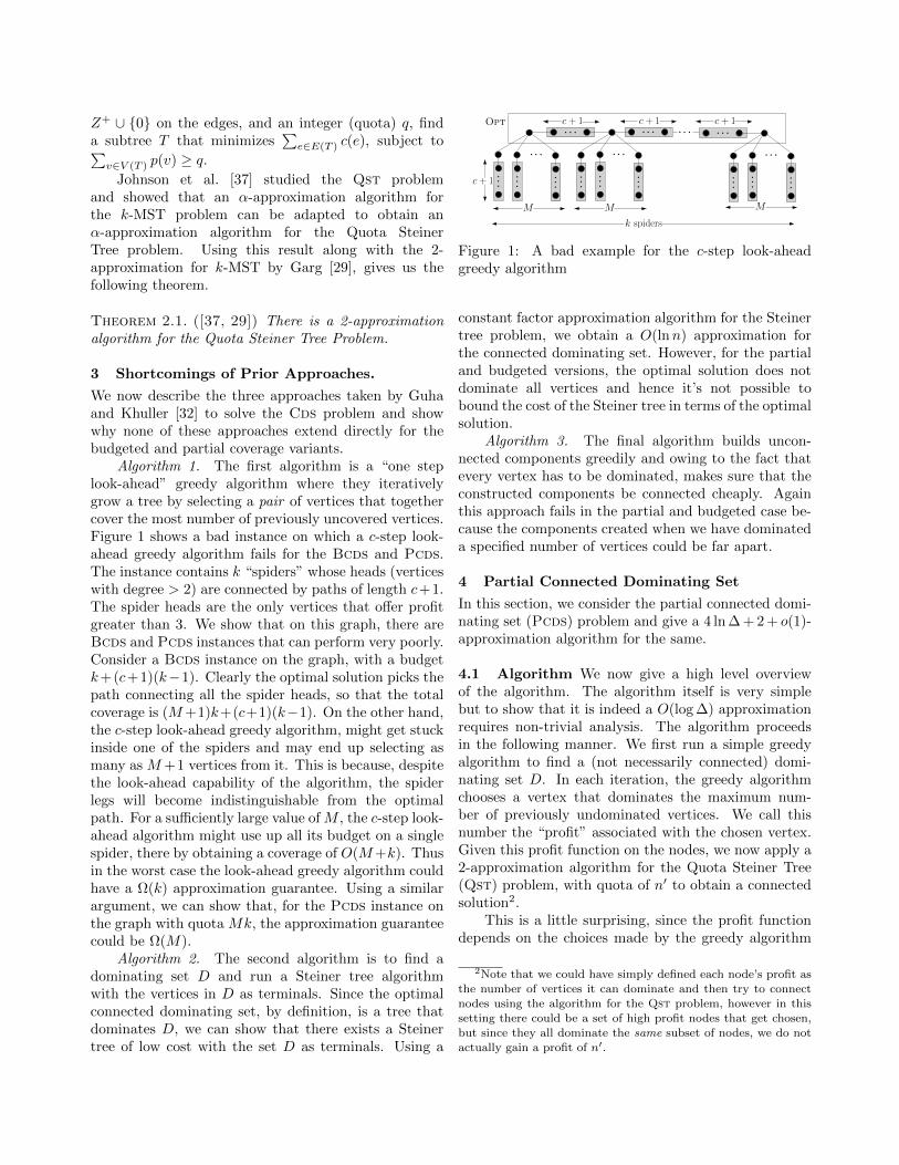
Algorithm 1. The first algorithm is a “one steplook-ahead” greedy algorithm where they iterativelygrow a tree by selecting a pair of vertices that togethercover the most number of previously uncovered vertices.Figure 1 shows a bad instance on which a c-step look-ahead greedy algorithm fails for the Bcds and Pcds.The instance contains k “spiders” whose heads (verticeswith degree > 2) are connected by paths of length c+1.The spider heads are the only vertices that offer profitgreater than 3. We show that on this graph, there areBcds and Pcds instances that can perform very poorly.Consider a Bcds instance on the graph, with a budgetk+(c+1)(k−1). Clearly the optimal solution picks thepath connecting all the spider heads, so that the totalcoverage is (M+1)k+(c+1)(k−1). On the other hand,the c-step look-ahead greedy algorithm, might get stuckinside one of the spiders and may end up selecting asmany as M+1 vertices from it. This is because, despitethe look-ahead capability of the algorithm, the spiderlegs will become indistinguishable from the optimalpath. For a sufficiently large value of M , the c-step look-ahead algorithm might use up all its budget on a singlespider, there by obtaining a coverage of O(M+k). Thusin the worst case the look-ahead greedy algorithm couldhave a Ω(k) approximation guarantee. Using a similarargument, we can show that, for the Pcds instance onthe graph with quota Mk, the approximation guaranteecould be Ω(M).

Algorithm 2. The second algorithm is to find adominating set D and run a Steiner tree algorithmwith the vertices in D as terminals. Since the optimalconnected dominating set, by definition, is a tree thatdominates D, we can show that there exists a Steinertree of low cost with the set D as terminals. Using a

M

c + 1

c + 1

c + 1 c + 1

M M

Opt

k spiders

Figure 1: A bad example for the c-step look-aheadgreedy algorithm

constant factor approximation algorithm for the Steinertree problem, we obtain a O(lnn) approximation forthe connected dominating set. However, for the partialand budgeted versions, the optimal solution does notdominate all vertices and hence it’s not possible tobound the cost of the Steiner tree in terms of the optimalsolution.

Algorithm 3. The final algorithm builds uncon-nected components greedily and owing to the fact thatevery vertex has to be dominated, makes sure that theconstructed components be connected cheaply. Againthis approach fails in the partial and budgeted case be-cause the components created when we have dominateda specified number of vertices could be far apart.

4 Partial Connected Dominating Set

In this section, we consider the partial connected domi-nating set (Pcds) problem and give a 4 ln ∆ + 2 + o(1)-approximation algorithm for the same.

4.1 Algorithm We now give a high level overviewof the algorithm. The algorithm itself is very simplebut to show that it is indeed a O(log ∆) approximationrequires non-trivial analysis. The algorithm proceedsin the following manner. We first run a simple greedyalgorithm to find a (not necessarily connected) domi-nating set D. In each iteration, the greedy algorithmchooses a vertex that dominates the maximum num-ber of previously undominated vertices. We call thisnumber the “profit” associated with the chosen vertex.Given this profit function on the nodes, we now apply a2-approximation algorithm for the Quota Steiner Tree(Qst) problem, with quota of n′ to obtain a connectedsolution2.

This is a little surprising, since the profit functiondepends on the choices made by the greedy algorithm

2Note that we could have simply defined each node’s profit as

the number of vertices it can dominate and then try to connectnodes using the algorithm for the Qst problem, however in thissetting there could be a set of high profit nodes that get chosen,

but since they all dominate the same subset of nodes, we do notactually gain a profit of n′.

in the first phase. However, we can show that thereis a subset of vertices D′ ⊆ D, of cardinality at most|Opt| ln ∆ + 1 whose profits sum up to at least n′

where |Opt| is the size of the optimum solution ofthe Pcds instance. Furthermore the vertices in D′

can be connected with additional (ln ∆ + 1)|Opt| + 1vertices. Thus, if we could find the smallest tree withtotal profit at least n′, such a tree would cost (numberof edges in the tree) no more than (2 ln ∆+1)|Opt|+1.This is a special case of the Qst problem (with unitedge costs) and hence we can apply Theorem 2.1 toobtain a tree of size (cost) no more than 2((2 ln ∆ +1)|Opt|+ 1) = (4 ln ∆ + 2)|Opt|+ 2. Thus, we obtaina (4 ln ∆ + 2 + o(1))-approximate solution for the Pcdsproblem.

Algorithm 4.1. Greedy Profit Labeling Algo-rithm for Pcds.Input: Graph G = (V,E) and n′ ∈ Z+ ∪ 0.Output: Tree T with at least n′ Coverage.

1: Compute the greedy dominating set D and thecorresponding profit function p : V → N using theAlgorithm 4.2.

2: Use the 2-approximation for Qst problem [37] onthe instance (G, p) to obtain a tree T with profit atleast n′.

Algorithm 4.2. Greedy Dominating Set.Input: Graph G = (V,E).Output: Dominating Set D and profit function p :V → Z+ ∪ 0.

1: D ← φ2: U ← V3: for all v ∈ V do4: p(v)← 0;5: end for6: while U 6= φ do7: v ← arg max

v∈V \D|NU (v)| . NU (v) is the set of

neighbors of v, including itself, in the set U8: Cv ← NU (v)9: p(v)← |Cv|

10: U ← U \NU (v)11: D ← D ∪ v12: end while

4.2 Analysis We first introduce some required nota-tion.

Notation: For every vertex v ∈ D that is chosenby the greedy algorithm, let Cv denote the set of new

vertices that v dominates i.e., we have p(v) = |Cv|. Wesay that v “covers” a vertex w if and only if w ∈ Cv.For the sake of analysis, we partition the vertices of thegraph G into layers. Let L1 = Opt be the vertices inan optimal solution for the Pcds instance, L2 be theset of vertices that are not in L1 and have at least oneneighbor in L1, and R = V \L1∪L2 be the remainingvertices. Let L3 be the subset of vertices of R that havea neighbor in L2. Furthermore let L′i = D∩Li, 1 ≤ i ≤ 3where D is the dominating set chosen by the greedyalgorithm. Figure 2 clarifies this notation regarding thelayers Li.

Figure 2: Pictorial Representation of Different Layers.(a) L1 is an optimal solution (b) L2 is set of the verticesadjacent to L1 (c) L3 is the subsequent layer (d) R is theset of all vertices other than L1∪L2 and (e) L′i = Li∩D.

We first show the following.

Lemma 4.1. There is a subset D′ ⊆ L′1 ∪ L′2 ∪ L′3 suchthat |D′| ≤ |Opt| ln ∆+1 and the total profit of verticesin D′ is at least n′, i.e.

∑v∈D′ p(v) ≥ n′.

Proof. Let L′1 ∪ L′2 ∪ L′3 = v1, v2, . . . , vl where thevertices are arranged according to the order in whichthey were selected by the greedy algorithm. Since allvertices in L1 ∪ L2 are dominated by L′1 ∪ L′2 ∪ L′3, we

have∑li=1 p(vi) ≥ |L1 ∪ L2| ≥ n′ where the second

inequality follows from the fact that L1 is a feasiblesolution (in fact optimal feasible solution). Choose t

such that∑ti=1 p(vi) < n′ and

∑t+1i=1 p(vi) ≥ n′. Let

S = v1, v2, . . . , vt denote the set of the first t verticeschosen from the set L′1 ∪ L′2 ∪ L′3. We now show that|S| = t ≤ |Opt| ln ∆ and hence D′ = S∪vt+1 satisfiesthe requirements of the claim.

Let C12 be the set of vertices in L1 ∪ L2 that arecovered by S in the original greedy step i.e., C12 =∪v∈SCv∩(L1∪L2). Let UC12 = (L1∪L2)\C12 be thevertices in L1 ∪L2 that are not covered by S. Similarlydefine CR = ∪v∈SCv ∩ R as the set of vertices in R

covered by S (as per the greedy step). Then, we havethat |CR| + |C12| < n′ ≤ |L1 ∪ L2| = |C12| + |UC12|,where the first inequality follows from the definition ofS. Therefore we have |CR| < |UC12|.

We can thus assign every vertex in CR to a uniquevertex in UC12, i.e. let I : CR → UC12 denote a oneto one function from CR to UC12. In the subsequentcharging argument, any cost that we charge to a vertexx ∈ CR is transferred to its assigned vertex I(x) ∈UC12. Hence, after this charge transfer, only verticesin L1 ∪ L2 will be charged. We will now use a chargingargument to show that |S| ≤ |Opt| ln ∆.

Consider a vertex u ∈ S. We recall that Cu is the setof vertices covered for the first time by u in the greedystep. We assign every w ∈ Cu a charge ρ(w) = 1

|Cu| .

It is clear that the total charge on all vertices is equalto the size of S. As described above, the charge of avertex in w ∈ R is transfered to its mapped vertex inI(w) ∈ UC12. Let v be a vertex in the optimal solutionset L1. We denote the set of neighbors of v, includingitself, by N (v). We claim that the total charge on thevertices of N (v) is at most ln ∆. Initially, none of thevertices in N (v) are charged. Let u1, u2 . . . , ul be thevertices in S which charge some vertices of N (v) in thatorder. This charge could either be the direct charge ora transfer of charge from some vertex in R. For i ∈ [l],let Oi ⊆ N (v) denote the set of vertices that remainuncharged (either directly or through a transfer), afterthe vertex ui is picked into S. Let O0 = N (v).

We will now show that, for every ui, |Cui | ≥ |Oi−1|.Let us consider the iteration of the greedy algorithm inwhich ui is picked. We claim that none of the vertices inOi−1 can be dominated by any vertex chosen before uiin the greedy algorithm. Let w ∈ Oi−1 be some vertexwhich is dominated by some vertex u′ chosen by greedybefore ui, such that w ∈ Cu′ . Clearly u′ ∈ L′1 ∪L′2 ∪L′3should hold, because no vertex in R\L3 can dominate w.But since u′ was chosen before ui and u′ ∈ L′1∪L′2∪L′3,u′ must be chosen into S before ui. Hence, w cannot bean uncharged vertex in the current iteration leading toa contradiction.

Thus, in the iteration where the greedy algorithmwas about to choose ui, none of the vertices Oi−1 havebeen dominated. Hence if the greedy were to choose v,then p(v) ≥ |Oi−1|. Since the greedy algorithm choosesvertex ui instead of v, we have |Cui

| ≥ |Oi−1|.The total charge in this iteration (Cui ∩ N (v)) is

thus at most |Oi−1|−|Oi||Oi−1| . Adding these charges over all

l iterations, we get, using an analysis very similar to theset cover analysis [19],

∑w∈N (v) ρ(w) ≤ H(∆), where

H is the harmonic function and ∆ is the maximumdegree. Adding up the charges over all vertices in L1,we get

∑u∈C12∪UC12

ρ(u) ≤∑v∈L1

∑w∈N (v) ρ(w) ≤

|Opt| ln ∆. Hence we have |S| ≤ |Opt| ln ∆. Since Swas a maximal set having profit at most n′, we obtaina set D′ with |D′| = |S| + 1 with profit at least n′ byadding a single vertex to S, which gives us the desiredresult.

Theorem 4.1. Let Opt be the optimal solution set foran instance of Pcds. There exists a tree T with at most2|Opt| ln ∆+|Opt|+1 edges such that

∑v∈T p(v) ≥ n′.

Proof. In Lemma 4.1, we have shown that there existsa subset D′ ⊆ L′1 ∪ L′2 ∪ L′3 of size |Opt| ln ∆ + 1 thathas profit at least n′. However this set D′ need notbe connected. We now show that this set D′ can beconnected without paying too much. Firstly we notethat for every vertex v ∈ L3 ∩D′, there exists a vertexw ∈ L2 such that w dominates v. Thus we can pick asubset D′′ ⊆ L2 of size at most |L3∩D′| ≤ |Opt| ln ∆+1which dominates all vertices of L3 ∩ D′. Now, it issufficient to ensure that all the vertices of (D′∩L2)∪D′′are connected. This can be achieved by simply addingall the vertices of L1 to our solution. Thus we haveshown that D = D′ ∪ D′′ ∪ L1 induces a connectedsubgraph with profit at least n′ and the number ofvertices in D ≤ |D′|+|D′′|+|L1| ≤ 2|Opt| ln ∆+|Opt|+2. Hence there exists subtree T on these vertices withat most (2 ln ∆ + 1)|Opt| + 1 edges with the requisitetotal profit.

Corollary 4.1. Algorithm 4.1 is a 4 ln ∆ + 2 + o(1)-approximation algorithm for Pcds.

Proof. Let Opt be the optimal solution of the Pcdsinstance. As per Theorem 4.1, we know that there existsa Steiner tree T with at most 2|Opt| ln ∆ + |Opt| + 1edges whose total profit exceeds the quota n′. Hence,the tree T returned by the 2-approximation for theQst problem has at most 4|Opt| ln ∆ + 2|Opt| + 2edges. Thus, we obtain a 4 ln ∆+2+o(1) approximationalgorithm.

5 Budgeted Connected Dominating Set

We now turn our attention to the Budgeted ConnectedDominating Set (Bcds) problem. We recall that in theBcds problem, we have to choose at most k vertices thatinduce a connected subgraph and maximize the numberof dominated vertices.

5.1 Algorithm Algorithm 5.1 is very similar to theone we used to obtain a partial connected dominatingset. We start by running the standard greedy algorithmto find a dominating set D in the graph. We set theprofits of vertices in D as the number of newly coveredvertices at each step of the greedy algorithm, while we

assign zero profit for the remaining vertices in V \ D.In the analysis section, we show that there is a treeon at most 3k vertices that has a total profit of atleast (1 − 1

e )Opt where Opt is the number of verticesdominated by an optimal solution. Note that we mayassume that we have guessed Opt by trying out valuesbetween k and n using, say, binary search. We runthe 2 approximation algorithm for the Quota Steinertree problem on this instance with the quota beingset to (1 − 1

e )Opt. This will result in a tree with atmost 6k nodes with total profit at least (1 − 1

e )Opt.Thus we obtain a (6, 1 − 1

e ) bicriteria approximationalgorithm. To convert this bicriteria approximationinto a true approximation, we use a dynamic program(Section 5.2.2) to find the “best” subtree on at most kvertices from this tree of 6k vertices. We use a simpletree decomposition scheme to show that the best treedominates at least 1

13 (1− 1e )Opt nodes.

Algorithm 5.1. Greedy Profit Labeling Algo-rithm for Bcds.Input: Graph G = (V,E) and k ∈ N.Output: Tree T with cost at most k.

1: Compute the greedy dominating set D and thecorresponding profit function p : V → N using theAlgorithm 4.2.

2: Opt← number of vertices dominated by an optimalsolution. . Guess using binary search between kand n

3: Use the 2-approximation for Qst problem [37] toobtain a tree T with profit at least (1− 1

e )Opt. .We show that |T | ≤ 6k.

4: Use the dynamic program of Section 5.2.2 to find T ,the best subtree of T having at most k vertices.

5.2 Analysis Let L1 denote the vertices in an opti-mal solution. Let layers L2, L3, R, and L′i be defined asin Section 4. Opt = |L1 ∪L2| is the number of verticesdominated by the optimal solution.

Let L′1∪L′2∪L′3 = v1, v2, . . . , vl where the verticesare according to the order in which they were selected bythe greedy algorithm. Let D′ = v1, v2, . . . , vk denotethe first k vertices from L′1∪L′2∪L′3. In Lemma 5.1, weprove that the total profit of D′ =

∑v∈D′ p(v) is at least

(1− 1e )Opt. Next, we can show that these k vertices can

be connected by using at most 2k more vertices, thusproving the existence of a tree with at most 3k verticeshaving the desired total profit.

Let gi denote the total profit after picking the firsti vertices from D′, i.e., gi =

∑ij=1 p(vj). We start by

proving that the following recurrence holds for everyi = 0 to k − 1.

Claim 1. gi+1 − gi ≥ 1k (Opt− gi)

Proof. Consider the iteration of the greedy algorithm,where vertex vi+1 is being picked. We first show thatat most gi vertices of L1 ∪ L2 have been already beendominated. Note that any vertex w ∈ L1 ∪ L2 that hasbeen already dominated must have been dominated bya vertex in v1, v2, . . . vi. This is because no vertex

from R \ L3 can neighbor w. Since gi =∑ij=1 p(vj)

is the total profit gained so far, it follows that at mostgi vertices from L1 ∪ L2 have been dominated. Hencewe have that there are at least Opt − gi undominatedvertices in L1 ∪ L2. Since the k vertices of L1 togetherdominate all of these, it follows that there exists at leastone vertex v ∈ L1 which neighbors at least 1

k (Opt− gi)undominated vertices.

We conclude this proof by noting that since thegreedy algorithm chose to pick vi+1 at this stage, insteadof the v above, it follows that p(vi+1) = gi+1 − gi ≥1k (Opt− gi).

Lemma 5.1. Let Opt be the number of vertices dom-inated by an optimal solution for Bcds. Then thereexists a subset D′ ⊆ D of size k with total profit at least(1− 1

e )Opt. Further, D′ can be connected using at most2k Steiner vertices.

Proof. From the Claim 1, the profit after i+1 iterationsis given by

gi+1 ≥Opt

k+ gi(1−

1

k).

By solving this recurrence, we get gi ≥ (1−(1− 1k )i)Opt.

Hence, we obtain the following.∑v∈D′

p(v) = gk ≥ (1− (1− 1

k)k)Opt ≥ (1− 1

e)Opt

We show that D′ can be connected by at most 2kSteiner nodes to form a connected tree. Note that forevery vertex v ∈ L3 ∩D′, there exists a vertex w ∈ L2

such that w neighbors v. Thus we can pick a subsetD′′ ⊆ L2 of size at most |L3 ∩D′| ≤ k which dominatesall vertices of L3∩D′. Now, it is sufficient to ensure thatall the vertices of (D′ ∩ L2) ∪ D′′ are connected. Thiscan be achieved by simply adding all the k vertices ofL1. Thus we have shown that D = D′∪D′′∪L1 inducesa connected subgraph with profit at least (1 − 1

e )Opt

and |D| ≤ |D′|+ |D′′|+ |L1| ≤ 3k.

Lemma 5.2. There is a (6, (1 − 1e )) bicriteria approxi-

mation algorithm for the Bcds problem.

Proof. Lemma 5.1 shows that there exists a Steiner treewith at most 3k vertices having total profit greater

than a quota of (1 − 1e )Opt. Hence, using the 2-

approximation for the Qst problem, we obtain a tree Tof at most 6k nodes and total profit at least (1− 1

e )Opt.Thus we obtain a (6, (1 − 1

e )) bicriteria approximationalgorithm for the Bcds problem.

5.2.1 Converting the Bicriteria Approximationto a True Approximation In order to obtain a trueapproximate solution (solution of size k), we need atechnique to find a small subtree T ⊆ T of k verticeswhich has high total profit. In Section 5.2.2, we showthat this problem can be easily solved in polynomialtime using dynamic programming. However, simplyfinding the subtree which maximizes the profit is notenough to give a good approximation ratio. We need away to compare the total profit of the subtree T withthe entire profit P =

∑v∈T p(v). We now show that if

n = 6k, we can obtain a subtree having profit at least113P .

The following lemma is well known in folklore andcan be easily proven by induction. It can also be seenas an easy consequence of a theorem by Jordan [38].

Lemma 5.3. (Jordan [38]) Given any tree on n ver-tices, we can decompose it into two trees (by replicatinga single vertex) such that the smaller tree has at most⌈n2

⌉nodes and the larger tree has at most

⌈2n3

⌉nodes.

We now show the following -

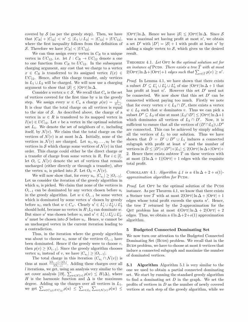
Lemma 5.4. Let k be greater than a sufficiently largeconstant. Given a tree T with 6k nodes, we candecompose it into 13 trees of size at most k nodes each.

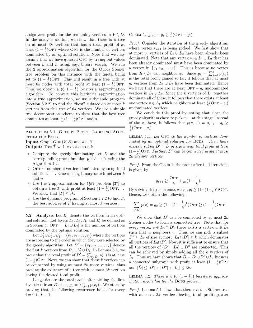
Proof. We use Lemma 5.3 to decompose the tree intotwo trees T1 and T2 such that |T1| ≤ |T2|. In this de-composition, at most one vertex is duplicated, therefore|T1| + |T2| ≤ 6k + 1. Also, we have |T1| ≤ 3k. We nowhave two cases:Case 1: |T1| ≥ 3k−1. In this case, |T2| ≤ 6k+1−|T1| ≤3k+2. Now repeatedly using Lemma 5.3 we can see thatT1 can be decomposed into at most 6 trees and T2 canbe decomposed into at most 7 trees of size at most k.This is shown in the Figure 3. Hence, in this case, wecan decompose the tree T into 13 trees.Case 2: |T1| ≤ 3k − 2. In this case, |T2| ≤ 4k. Inthis case, we can decompose T1 into 5 trees and T2 canbe decomposed into 8 trees. This is shown in Figure 4.Thus in this case, we can decompose T into 13 trees.

Using Lemma 5.4, we can convert the bicriteria approx-imation for Bcds to a true approximation algorithm.In particular, we show the following -

Theorem 5.1. There is a 113 (1 − 1

e ) approximationalgorithm for the Bcds problem.

Figure 3: First tree decomposes into 6 subtrees andsecond tree decomposes into 7 trees. In total, we obtain13 subtrees. The number associated with each node isthe upper bound on the size of the subtree.

Proof. By Lemma 5.2, we obtain a tree T with at most6k nodes with profit (1− 1

e )Opt. Now using Lemma 5.4,we obtain 13 trees in the worst case, say T1, T2, . . . T13.Finally, out of these 13 trees (each of size at most k),we pick the tree T with the highest total profit. Let,p(T ) =

∑v∈T p(v) denote the total profit of tree T .

Then we have,

p(T ) ≥ 1

13

13∑i=1

p(Ti) ≥1

13p(T ) ≥ 1

13(1− 1

e)Opt

Thus we have a 113 (1− 1

e ) approximation guarantee.

5.2.2 Finding the Best Subtree Although the de-composition Lemma 5.4 is useful to prove a theoreti-cal bound, from a practical perspective it is better touse a dynamic programming approach to find the bestk sub-tree. Formally, we have the following problem.Given a tree T = (V,E) of n vertices, profits on ver-tices p : V → Z+ ∪ 0, and an integer k, find a sub-tree T of k vertices which maximizes the total profitP =

∑v∈T p(v). We show that this problem can be

solved in polynomial time using dynamic programming.Let the tree T be rooted at an arbitrary vertex and Tvdenote the subtree rooted at a vertex v. We define thefollowing -

Figure 4: First tree decomposes into 5 subtrees andsecond tree decomposes into 8 trees. In total, we obtain13 subtrees. The number associated with each node isthe upper bound on the size of the subtree.

F (v, i) ← best solution of at most i vertices com-pletely contained inside Tv.

G(v, i) ← best solution of at most i vertices com-pletely contained inside Tv such that v is a part of thesolution.

The desired solution is thus at F (root, k). The basecases (when v is a leaf) are trivial. Let v1, v2, . . . , vldenote the children of vertex v. We now have thefollowing recurrence -

F (v, i) = max

max1≤j≤l

F (vj , i), G(v, i)

G(v, i) = p(v) +M(l, i− 1)

where M(j, i′) denotes the best way to distribute abudget of i′ among the first j children of v. In otherwords,

M(l, i− 1) = maxi1+i2+...+il=i−1

∑j

G(vj , ij)

M(j, i′) is computed using another dynamic program asfollows. Again the base cases when j = 0 or i′ = 0 aretrivial. For 1 ≤ j ≤ l and 1 ≤ i′ ≤ i − 1, we have the

following recurrence -

M(j, i′) = max0≤i∗≤i′

M(j − 1, i∗) +G(vj , i′ − i∗)

6 Budgeted Generalized Cds

In this section, we show that our approach extends tomore general budgeted connected domination problems.Formally, given a graph G = (V,E), a budget k, and amonotone special submodular profit function f : 2V →Z+∪0, find a subset S ⊆ V which maximizes f(S) suchthat |S| ≤ k and induces a connected subgraph of G.As mentioned earlier in Section 2, this problem capturesthe budgeted variants of the capacitated and weightedprofit connected dominating set problems.

6.1 Algorithm. Algorithm 6.1 begins by runningthe standard greedy algorithm to find a basis of thepolymatroid associated with f . In other words, wegreedily pick a vertex v with the maximum marginalprofit f(D ∪ v) − f(D) until all vertices have zeromarginal profit. With every selected vertex, we as-sociate the marginal profit gained, and associate zeroprofit with the other vertices. Finally, we run a quotaSteiner tree algorithm using these profits to find thesmallest tree that yields a profit of at least (1− 1

e )Optwhere Opt is the optimal profit (which we guess). Inthe analysis section, we show that there exists a tree Tof size at most 3k with f(T ) ≥ (1 − 1

e )Opt. Hence,the 2-approximation for the quota Steiner tree yields atree T of size at most 6k yielding the desired profit. Fi-nally using the tree decomposition described earlier, weshow that we can obtain a tree T of size at most k withf(T ) ≥ 1

13 (1− 1e )Opt.

6.2 Analysis. Let the L1 denote the vertices in theoptimal solution and f(L1) = Opt. Let L2 denotethe set of vertices which have at least one neighborin L1, and similarly let L3 denote the set of verticeshaving a neighbor in L2 (and NOT in L1). Let R =V \ L1 ∪ L2 ∪ L3 denote the rest of the vertices. LetL′i = D∩Li where D is the set of vertices chosen by thegreedy algorithm.

Further, let D′ denote the first k vertices picked bythe greedy algorithm from L′1 ∪ L′2 ∪ L′3. To simplifynotation, let D′ = v1, v2, . . . , vk and let Di denotethe the set of vertices already picked by the greedyalgorithm when the vertex vi+1 is being chosen. Hencewe have vi+1 = arg maxv∈V \Di

f(Di ∪ v) − f(Di)and p(vi+1) = f(Di ∪ vi+1) − f(Di). Note that inparticular Di ⊆ D but may not be a subset of D′. Alsolet D′i = ∪ij=1vj denote the first i vertices in D′. LetP (D′i) =

∑v∈D′i

p(v) denote the total profit associated

with the set D′i. Finally let D′′i = Di\D′i be the vertices

in Di ∩R.

Claim 2. p(vi+1) = P (D′i+1) − P (D′i) ≥ 1k (Opt −

P (D′i))

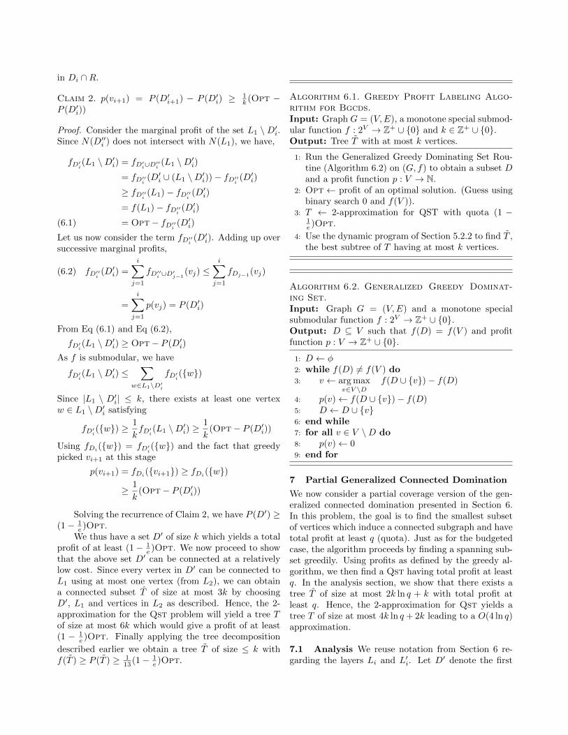
Proof. Consider the marginal profit of the set L1 \D′i.Since N(D′′i ) does not intersect with N(L1), we have,

fD′i(L1 \D′i) = fD′i∪D′′i (L1 \D′i)= fD′′i (D′i ∪ (L1 \D′i))− fD′′i (D′i)

≥ fD′′i (L1)− fD′′i (D′i)

= f(L1)− fD′′i (D′i)

= Opt− fD′′i (D′i)(6.1)

Let us now consider the term fD′′i (D′i). Adding up oversuccessive marginal profits,

fD′′i (D′i) =

i∑j=1

fD′′i ∪D′j−1(vj) ≤

i∑j=1

fDj−1(vj)(6.2)

=

i∑j=1

p(vj) = P (D′i)

From Eq (6.1) and Eq (6.2),

fD′i(L1 \D′i) ≥ Opt− P (D′i)

As f is submodular, we have

fD′i(L1 \D′i) ≤∑

w∈L1\D′i

fD′i(w)

Since |L1 \ D′i| ≤ k, there exists at least one vertexw ∈ L1 \D′i satisfying

fD′i(w) ≥1

kfD′i(L1 \D′i) ≥

1

k(Opt− P (D′i))

Using fDi(w) = fD′i(w) and the fact that greedypicked vi+1 at this stage

p(vi+1) = fDi(vi+1) ≥ fDi

(w)

≥ 1

k(Opt− P (D′i))

Solving the recurrence of Claim 2, we have P (D′) ≥(1− 1

e )Opt.We thus have a set D′ of size k which yields a total

profit of at least (1− 1e )Opt. We now proceed to show

that the above set D′ can be connected at a relativelylow cost. Since every vertex in D′ can be connected toL1 using at most one vertex (from L2), we can obtaina connected subset T of size at most 3k by choosingD′, L1 and vertices in L2 as described. Hence, the 2-approximation for the Qst problem will yield a tree Tof size at most 6k which would give a profit of at least(1 − 1

e )Opt. Finally applying the tree decomposition

described earlier we obtain a tree T of size ≤ k withf(T ) ≥ P (T ) ≥ 1

13 (1− 1e )Opt.

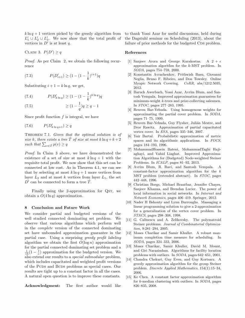
Algorithm 6.1. Greedy Profit Labeling Algo-rithm for Bgcds.Input: Graph G = (V,E), a monotone special submod-ular function f : 2V → Z+ ∪ 0 and k ∈ Z+ ∪ 0.Output: Tree T with at most k vertices.

1: Run the Generalized Greedy Dominating Set Rou-tine (Algorithm 6.2) on (G, f) to obtain a subset Dand a profit function p : V → N.

2: Opt← profit of an optimal solution. (Guess usingbinary search 0 and f(V )).

3: T ← 2-approximation for QST with quota (1 −1e )Opt.

4: Use the dynamic program of Section 5.2.2 to find T ,the best subtree of T having at most k vertices.

Algorithm 6.2. Generalized Greedy Dominat-ing Set.Input: Graph G = (V,E) and a monotone specialsubmodular function f : 2V → Z+ ∪ 0.Output: D ⊆ V such that f(D) = f(V ) and profitfunction p : V → Z+ ∪ 0.

1: D ← φ2: while f(D) 6= f(V ) do3: v ← arg max

v∈V \Df(D ∪ v)− f(D)

4: p(v)← f(D ∪ v)− f(D)5: D ← D ∪ v6: end while7: for all v ∈ V \D do8: p(v)← 09: end for

7 Partial Generalized Connected Domination

We now consider a partial coverage version of the gen-eralized connected domination presented in Section 6.In this problem, the goal is to find the smallest subsetof vertices which induce a connected subgraph and havetotal profit at least q (quota). Just as for the budgetedcase, the algorithm proceeds by finding a spanning sub-set greedily. Using profits as defined by the greedy al-gorithm, we then find a Qst having total profit at leastq. In the analysis section, we show that there exists atree T of size at most 2k ln q + k with total profit atleast q. Hence, the 2-approximation for Qst yields atree T of size at most 4k ln q+ 2k leading to a O(4 ln q)approximation.

7.1 Analysis We reuse notation from Section 6 re-garding the layers Li and L′i. Let D′ denote the first

k ln q + 1 vertices picked by the greedy algorithm fromL′1 ∪ L′2 ∪ L′3. We now show that the total profit ofvertices in D′ is at least q.

Claim 3. P (D′) ≥ q

Proof. As per Claim 2, we obtain the following recur-rence

P (D′i+1) ≥ (1− (1− 1

k)i+1)q(7.3)

Substituting i+ 1 = k ln q, we get,

P (D′k ln q) ≥ (1− (1− 1

k)k ln q)q(7.4)

≥ (1− 1

q)q ≥ q − 1(7.5)

Since profit function f is integral, we have

P (D′k ln q+1) ≥ q(7.6)

Theorem 7.1. Given that the optimal solution is ofsize k, there exists a tree T of size at most k ln q+k+ 2such that

∑v∈T p(v) ≥ q

Proof. In Claim 3 above, we have demonstrated theexistence of a set of size at most k ln q + 1 with therequisite total profit. We now show that this set can beconnected at low cost. As in Theorem 4.1, we can seethat by selecting at most k ln q + 1 more vertices fromlayer L2 and at most k vertices from layer L1, the setD′ can be connected to form a tree T .

Finally using the 2-approximation for Qst, weobtain a O(4 ln q) approximation.

8 Conclusion and Future Work

We consider partial and budgeted versions of thewell studied connected dominating set problem. Weobserve that various algorithms which perform wellin the complete version of the connected dominatingset have unbounded approximation guarantee in thepartial case. Using a surprising greedy profit labelingalgorithm we obtain the first O(log n) approximationfor the partial connected dominating set problem and a113 (1 − 1

e ) approximation for the budgeted version. Wealso extend our results to a special submodular problem,which includes capacitated and weighted profit versionsof the Pcds and Bcds problems as special cases. Ourresults are tight up to a constant factor in all the cases.A natural open question is to improve these constants.

Acknowledgment: The first author would like

to thank Yossi Azar for useful discussions, held duringthe Dagstuhl seminar on Scheduling (2013), about thefailure of prior methods for the budgeted Cds problem.

References

[1] Sanjeev Arora and George Karakostas. A 2 + εapproximation algorithm for the k-MST problem. InSODA, pages 754–759, 2000.

[2] Konstantin Avrachenkov, Prithwish Basu, GiovanniNeglia, Bruno F. Ribeiro, and Don Towsley. OnlineMyopic Network Covering. CoRR, abs/1212.5035,2012.

[3] Baruch Awerbuch, Yossi Azar, Avrim Blum, and San-tosh Vempala. Improved approximation guarantees forminimum-weight k-trees and prize-collecting salesmen.In STOC, pages 277–283, 1995.

[4] Reuven Bar-Yehuda. Using homogenous weights forapproximating the partial cover problem. In SODA,pages 71–75, 1999.

[5] Reuven Bar-Yehuda, Guy Flysher, Julian Mestre, andDror Rawitz. Approximation of partial capacitatedvertex cover. In ESA, pages 335–346, 2007.

[6] Yair Bartal. Probabilistic approximation of metricspaces and its algorithmic applications. In FOCS,pages 184–193, 1996.

[7] MohammadHossein Bateni, MohammadTaghi Haji-aghayi, and Vahid Liaghat. Improved Approxima-tion Algorithms for (Budgeted) Node-weighted SteinerProblems. In ICALP, pages 81–92, 2013.

[8] Avrim Blum, R. Ravi, and Santosh Vempala. Aconstant-factor approximation algorithm for the kMST problem (extended abstract). In STOC, pages442–448, 1996.

[9] Christian Borgs, Michael Brautbar, Jennifer Chayes,Sanjeev Khanna, and Brendan Lucier. The power oflocal information in social networks. In Internet andNetwork Economics, pages 406–419. Springer, 2012.

[10] Nader H Bshouty and Lynn Burroughs. Massaging alinear programming solution to give a 2-approximationfor a generalization of the vertex cover problem. InSTACS, pages 298–308, 1998.

[11] G. Calinescu and A. Zelikovsky. The polymatroidSteiner problems. Journal of Combinatorial Optimiza-tion, 9:281–294, 2005.

[12] Moses Charikar and Samir Khuller. A robust max-imum completion time measure for scheduling. InSODA, pages 324–333, 2006.

[13] Moses Charikar, Samir Khuller, David M. Mount,and Giri Narasimhan. Algorithms for facility locationproblems with outliers. In SODA, pages 642–651, 2001.

[14] Chandra Chekuri, Guy Even, and Guy Kortsarz. Agreedy approximation algorithm for the group Steinerproblem. Discrete Applied Mathematics, 154(1):15–34,2006.

[15] Ke Chen. A constant factor approximation algorithmfor k-median clustering with outliers. In SODA, pages826–835, 2008.

[16] Maggie X Cheng, Lu Ruan, and Weili Wu. Achiev-ing minimum coverage breach under bandwidth con-straints in wireless sensor networks. In INFOCOM,pages 2638–2645, 2005.

[17] Maggie X Cheng, Lu Ruan, and Weili Wu. Coveragebreach problems in bandwidth-constrained sensor net-works. TOSN, page 12, 2007.

[18] Xiuzhen Cheng, Xiao Huang, Deying Li, Weili Wu,and Ding-Zhu Du. A polynomial-time approximationscheme for the minimum-connected dominating set inad hoc wireless networks. Networks, 42(4):202–208,2003.

[19] Thomas H. Cormen, Charles E. Leiserson, Ronald L.Rivest, and Clifford Stein. Introduction to Algorithms,3rd Edition. page 977, 2009.

[20] Bevan Das and Vaduvur Bharghavan. Routing in ad-hoc networks using minimum connected dominatingsets. In IEEE International Conference on Communi-cations (ICC), volume 1, pages 376–380. IEEE, 1997.

[21] Erik D Demaine and MohammadTaghi Hajiaghayi.Bidimensionality: New Connections between FPT al-gorithms and PTASs. In SODA, pages 590–601, 2005.

[22] D.Z. Du and P.J. Wan. Connected Dominating Set:Theory and Applications. Springer Optimization andIts Applications. Springer New York, 2013.

[23] Devdatt P. Dubhashi, Alessandro Mei, AlessandroPanconesi, Jaikumar Radhakrishnan, and AravindSrinivasan. Fast distributed algorithms for (weakly)connected dominating sets and linear-size skeletons. InSODA, pages 717–724, 2003.

[24] Jittat Fakcharoenphol, Satish Rao, and Kunal Talwar.A tight bound on approximating arbitrary metrics bytree metrics. In STOC, pages 448–455, 2003.

[25] Uriel Feige. A threshold of lnn for approximating setcover. J. ACM, 45(4):634–652, July 1998.

[26] Rajiv Gandhi, Samir Khuller, and Aravind Srinivasan.Approximation algorithms for partial covering prob-lems. J. Algorithms, 53(1):55–84, 2004.

[27] Rajiv Gandhi and Srinivasan Parthasarathy. Dis-tributed algorithms for connected domination in wire-less networks. Journal of Parallel and DistributedComputing, 67(7):848–862, 2007.

[28] Naveen Garg. A 3-approximation for the minimum treespanning k vertices. In FOCS, pages 302–309, 1996.

[29] Naveen Garg. Saving an epsilon: a 2-approximationfor the k-MST problem in graphs. In STOC, pages396–402, 2005.

[30] Naveen Garg, Goran Konjevod, and R. Ravi. A Poly-logarithmic Approximation Algorithm for the GroupSteiner Tree Problem. In SODA, pages 253–259, 1998.

[31] Teofilo F. Gonzalez. Clustering to Minimize the Max-imum Intercluster Distance. Theor. Comput. Sci.,38:293–306, 1985.

[32] Sudipto Guha and Samir Khuller. Approximation al-gorithms for connected dominating sets. Algorithmica,20(4):374–387, 1998.

[33] Anupam Gupta, Ravishankar Krishnaswamy, AmitKumar, and Danny Segev. Scheduling with Outliers.

In APPROX-RANDOM, pages 149–162, 2009.[34] Eran Halperin and Robert Krauthgamer. Polylogarith-

mic inapproximability. In STOC, pages 585–594, 2003.[35] Eran Halperin and Aravind Srinivasan. Improved ap-

proximation algorithms for the partial vertex coverproblem. In Approximation Algorithms for Combina-torial Optimization, pages 161–174. 2002.

[36] Dorit S Hochbaum and David B Shmoys. A unifiedapproach to approximation algorithms for bottleneckproblems. Journal of the ACM (JACM), 33(3):533–550, 1986.

[37] David S Johnson, Maria Minkoff, and Steven Phillips.The prize collecting Steiner tree problem: theory andpractice. In SODA, pages 760–769, 2000.

[38] Camille Jordan. Sur les assemblages de lignes. Journalfur die reine und angewandte Mathematik, 70:185–190,1869.

[39] Michael J Kearns. The computational complexity ofmachine learning. The MIT Press, 1990.

[40] Samir Khuller, Anna Moss, and Joseph (Seffi) Naor.The budgeted maximum coverage problem. Informa-tion Processing Letters, 70(1):39 – 45, 1999.

[41] Samir Khuller, Barna Saha, and Kanthi K Sarpatwar.New Approximation Results for Resource ReplicationProblems. In APPROX-RANDOM, pages 218–230.2012.

[42] Yuzhen Liu and Weifa Liang. Approximate coverage inwireless sensor networks. In ICN, pages 68–75, 2005.

[43] Julian Mestre. A primal-dual approximation algorithmfor partial vertex cover: Making educated guesses.Algorithmica, 55(1):227–239, 2009.

[44] Anna Moss and Yuval Rabani. Approximation algo-rithms for constrained for constrained node weightedSteiner tree problems. In STOC, pages 373–382, 2001.

[45] George L Nemhauser, Laurence A Wolsey, and Mar-shall L Fisher. An analysis of approximations for max-imizing submodular set functions I. Mathematical Pro-gramming, 14(1):265–294, 1978.

[46] R. Ravi, R. Sundaram, M. V. Marathe, D. J.Rosenkrantz, and S. S. Ravi. Spanning Trees—Shortor Small. SIAM J. Discret. Math., 9(2):178–200, May1996.

[47] Petr Slavık. Improved performance of the greedyalgorithm for partial cover. Information ProcessingLetters, 64(5):251–254, 1997.

[48] Aravind Srinivasan. Distributions on level-sets withapplications to approximation algorithms. In FOCS,pages 588–597, 2001.

[49] Peng-Jun Wan, Khaled M Alzoubi, and Ophir Frieder.Distributed construction of connected dominating setin wireless ad hoc networks. In INFOCOM, volume 3,pages 1597–1604, 2002.

[50] Laurence A. Wolsey. An analysis of the greedy algo-rithm for the submodular set covering problem. Com-binatorica, 2(4):385–393, 1982.

[51] Jie Wu and Hailan Li. On calculating connecteddominating set for efficient routing in ad hoc wirelessnetworks. In DIALM, pages 7–14, 1999.