Analyzing the Relationship between Income Inequality and Economic Growth:

Paravee Meneejuk and Woraphon Yamaka

Does the Kuznets Curve Exist in Thailand?

2

1 2 4

5

Introduction &Literature Reviews:Motivation of this research

Methodology Model Specification and Variables

Data

3

Simulation Study

6 7

Empirical Results Conclusion

Contents

Introduction

The relationship between income disparity and economic growth is a critical issue in macroeconomics.

Every country needs economic growth

3

for improving standard of living

for reducing a povertyfor surviving in the modern economy

e.g. Technology progress which is a major source of economic growth may cause the higher inequality of income. The increase in demand for skilled workers, relatively greater compared to unskilled workers owing to the technological development, is likely to widen the inequality of income. (Acemoglu, 1998)

but a rise in growth can also cause income inequality.

Introduction

While income inequality is considered to be a consequence of economic growth, there is also the argument that the inequality may affect the growth at the same time andperhaps it is necessary to propel the growth.

4

“Two sides of the same coin”is what Ostry and Berg, IMF staff, used to define the effect of inequality on economic growth.(Ostry and Berg, 2011)

Introduction

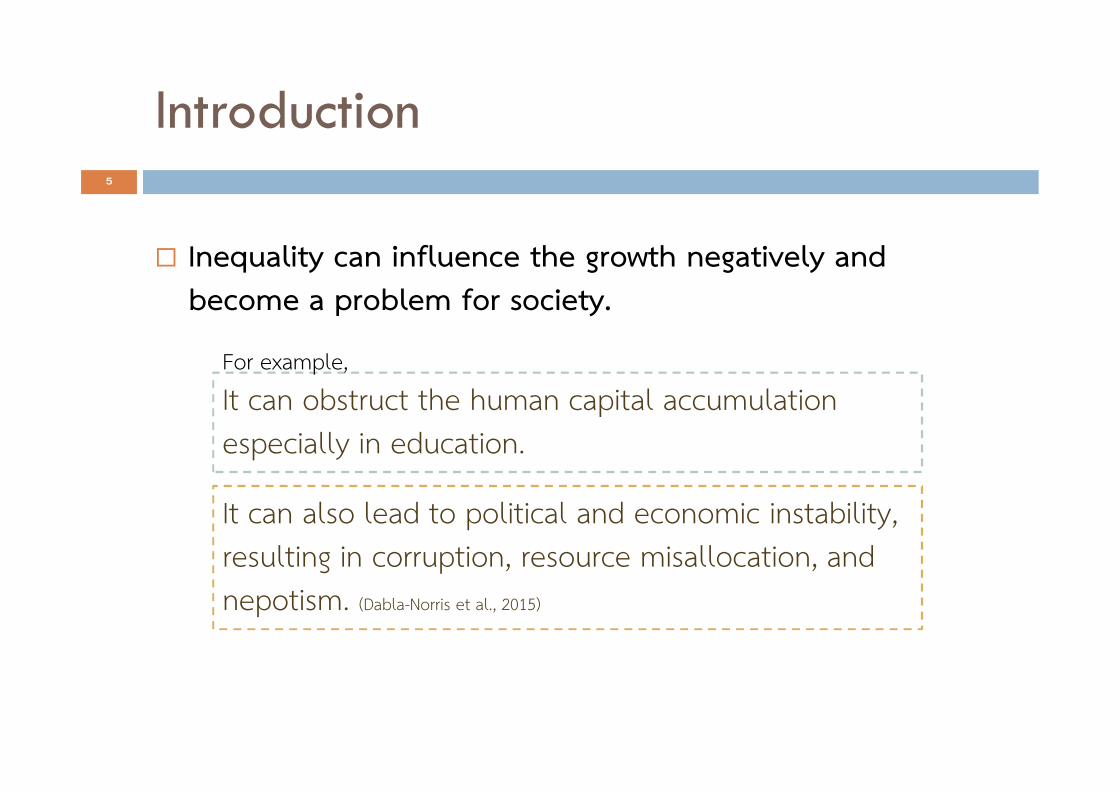
Inequality can influence the growth negatively and become a problem for society.

5

It can obstruct the human capital accumulation especially in education.

It can also lead to political and economic instability, resulting in corruption, resource misallocation, and nepotism. (Dabla-Norris et al., 2015)

For example,

Introduction

In contrast, inequality can also be good for economy since it provides incentives for people to invest and save for their future livelihood and also for entrepreneurs to run their businesses successfully.

6

incentives

Trade-off between Increasing Growth and Reducing Inequality

7

Ineq

ualit

y

Income per Capita

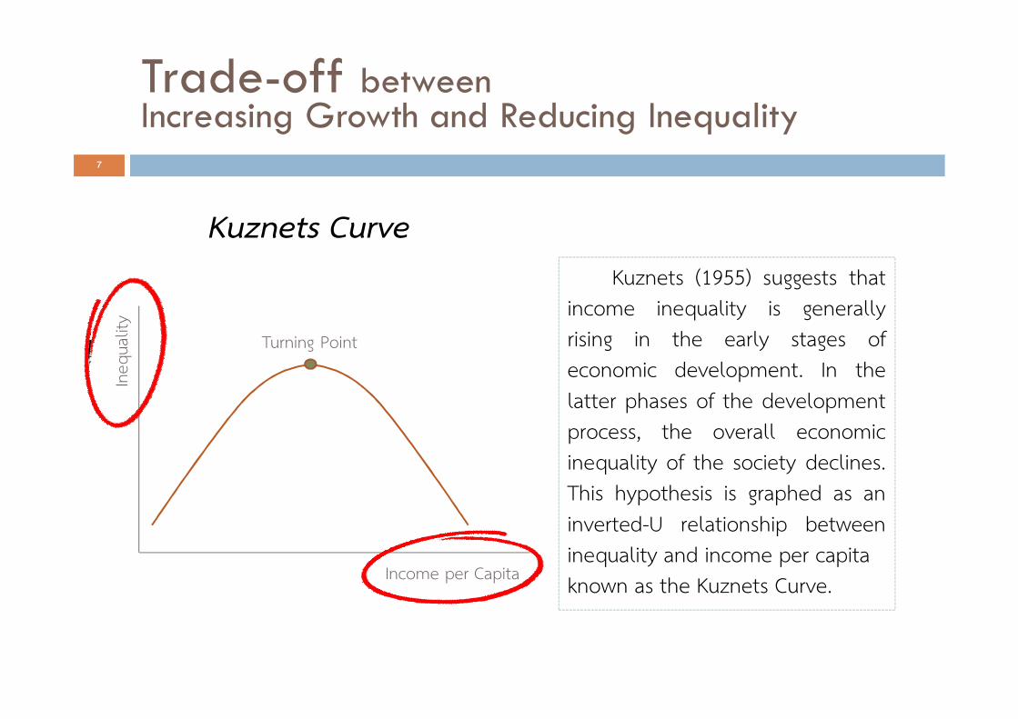
Kuznets (1955) suggests that income inequality is generally rising in the early stages of economic development. In the latter phases of the development process, the overall economic inequality of the society declines. This hypothesis is graphed as an inverted-U relationship between inequality and income per capitaknown as the Kuznets Curve.

Kuznets Curve

Turning Point

Research Question8

We aims to investigate whether the Kuznets hypothesis holds in Thailand’s economic system. If this hypothesis holds, we then aim to find the threshold or the proper rate of economic growth that will not hurt income distribution in the long term.

Does the Kuznets Curve Exist in Thailand

Literature Reviews9

The first group is the empirical evidences that clearly accept the Kuznets hypothesis in favor of the inverted-U relationship between income inequality and economic growth.

The second group is the studies that reject this hypothesis or find the nonexistence of the Kuznets curve.

For example, the study of Heshmati (2004), Khalifa and El Hag (2010), and Ogus (2012).

For example, the study of Hsing and Smyth (1994), Deininger and Squire (1996), Easterly (1999), Dollar and Kraay(2002)

Literature Reviews10

The study about Kuznets Curve in Thailand

As in the literature, many studies paid attention on an investigating of the Kuznets hypothesis in Thailand. Many of them are failed to find this inverted-U relationship such as Gallup (2012) whereas some are not. Some studies could find a little support for the Kuznets hypothesis in Thailand.

For example, the study of Ikemoto and Uehara (2000), Noppakhun (2007), Preechametta (2015), and พงษธร วราศัย(2558)

What do we notice from the literature reviews?11

Most of the studies are limited by the lack of the efficient statistical tools.

- Some studies decided to split the observation into two groups and estimate each part separately to get coefficients.

- These regression results in testing the inverted-U hypothesis were estimated only by parametric forms which produce strictly concave functions.

- The existing studies typically relied on a linear regression and the linear rigid quadratic regression model e.g. ARDL, ECM.

What do we notice from the literature reviews?12

A better way to investigate the Kuznets Curve

Savvides and Stegnos (2000) suggested using a threshold regression model to perform a test of inverted-U hypothesis. This model is in favor of nonlinear model which help us achieve the test without splitting the observation to estimate different coefficients.

Drawback of this method

The functional form of the threshold model is discontinuity.

What is the contribution of our paper?13

The main contribution in terms of Econometrics

The main contribution in terms of Economics

We propose a new approach to investigate the inverted-U relationship; an innovative tool that overcomes the drawback of the previous method, called a smooth Kink regression.

We investigate the existence of Kuznets curve in Thailand with efficient tool. If we can prove that the hypothesis holds and the result can illustrate the turning point accurately, it means we can find the proper rate of economic growth that will not hurt income distribution in the long term. Our findings should be useful for the Thai government and policy makers and can contribute to longer-run benefits for society.

14

1 2 4

5

Introduction &Literature Reviews:Motivation of this research

Methodology Model Specification and Variables

Data

3

Simulation Study

6 7

Empirical Results Conclusion

Contents

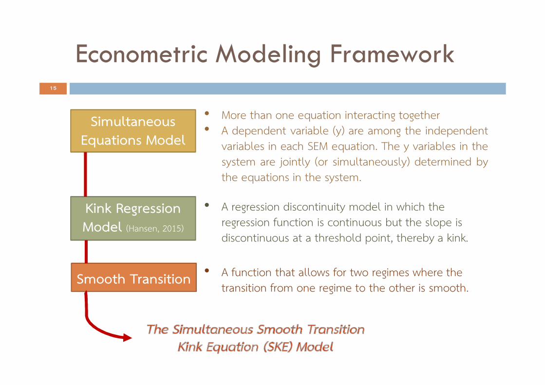
Econometric Modeling Framework15

Simultaneous Equations Model

Kink Regression Model (Hansen, 2015)

Smooth Transition

• More than one equation interacting together • A dependent variable (y) are among the independent

variables in each SEM equation. The y variables in the system are jointly (or simultaneously) determined by the equations in the system.

• A regression discontinuity model in which the regression function is continuous but the slope is discontinuous at a threshold point, thereby a kink.

• A function that allows for two regimes where the transition from one regime to the other is smooth.

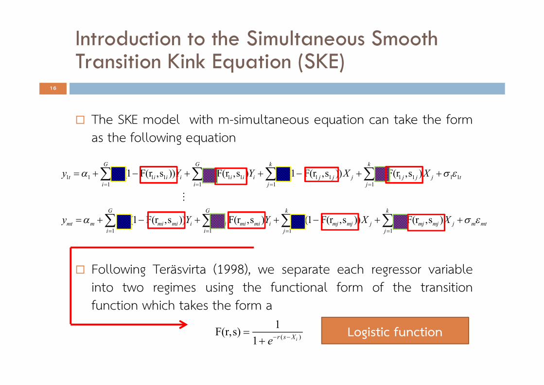
Introduction to the Simultaneous Smooth Transition Kink Equation (SKE)

16

The SKE model with m-simultaneous equation can take the form as the following equation

Following Teräsvirta (1998), we separate each regressor variable into two regimes using the functional form of the transition function which takes the form a

1 1 1 1 1 1 1 1 1 1 1 1 1 1 1 11 1 1 1

1 1 1

(1 F(r ,s )) F(r ,s ) (1 F(r ,s )) F(r ,s )

(1 F(r ,s )) F(r ,s ) (1 F(r ,s )) F(r ,

G G k k

t i i i i i i i i j j j j j j j j ti i j j

G G k

mt m mi mi mi i mi mi mi i mj mj mj j mj mji i j

y Y Y X X

y Y Y X

1

s )k

mj j m mtj

X

( )

1F(r,s)1 ir s Xe

Logistic function

Copula Approach17

Copulas are parametrically specified joint distributions which are generated from any given marginal distributions. The main advantage of copulas is that it can separate the marginal behavior and the dependence structure of the variables from their joint distribution function. Copula is used to model the dependence structure of the SKE model.

The Elliptical class: the symmetric Gaussian and t-Copula. The Archimedean class: the Gumbel, Frank, Clayton, and Joe. 1 2 1 2( , ) ( ( ), ( ))C u u C F G

1 1u 2 2u

18

1 2 4

5

Introduction &Literature Reviews:Motivation of this research

Methodology Model Specification and Variables

Data

3

Simulation Study

6 7

Empirical Results Conclusion

Contents

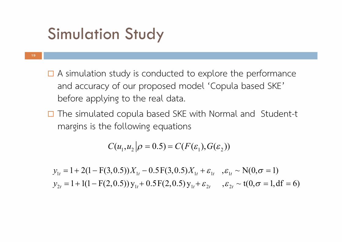
Simulation Study19

A simulation study is conducted to explore the performance and accuracy of our proposed model ‘Copula based SKE’ before applying to the real data.

The simulated copula based SKE with Normal and Student-t margins is the following equations

1 2 1 2( , 0.5) ( ( ), ( ))C u u C F G

1 1 1 1 1

2 1 1 2 2

1 2(1 F(3,0.5)) 0.5F(3,0.5) , ~ N(0, 1)1 1(1 F(2,0.5)) y 0.5F(2,0.5) y , ~ t(0, 1,df 6)

t t t t t

t t t t t

y X Xy

20

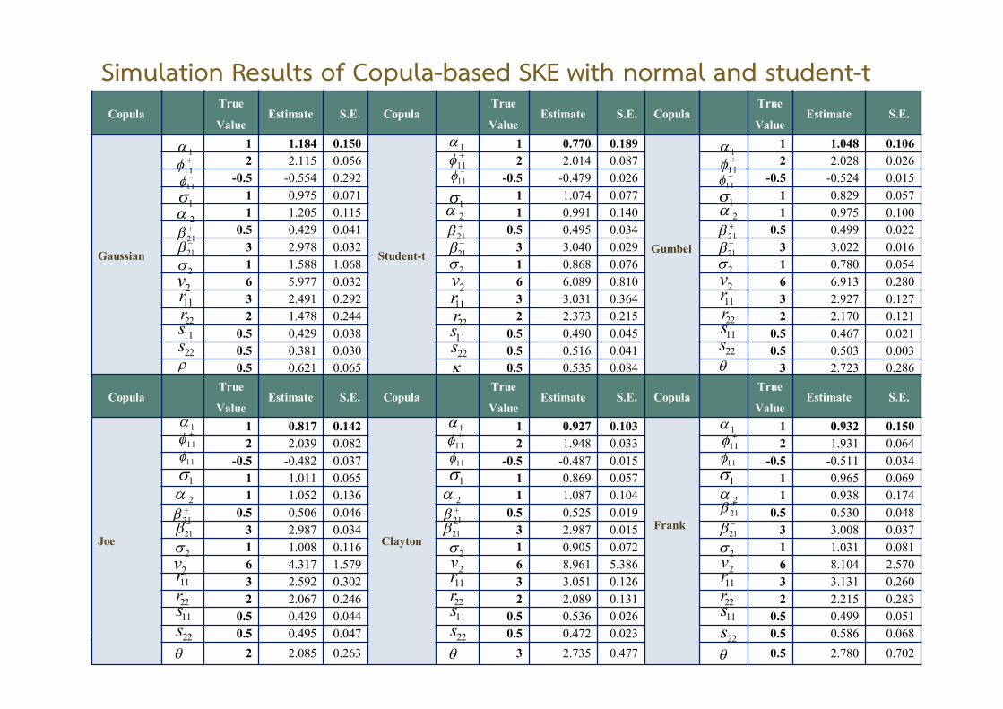
CopulaTrue

ValueEstimate S.E. Copula

True

ValueEstimate S.E. Copula

True

ValueEstimate S.E.

Gaussian

1 1.184 0.150

Student-t

1 0.770 0.189

Gumbel

1 1.048 0.1062 2.115 0.056 2 2.014 0.087 2 2.028 0.026

-0.5 -0.554 0.292 -0.5 -0.479 0.026 -0.5 -0.524 0.0151 0.975 0.071 1 1.074 0.077 1 0.829 0.0571 1.205 0.115 1 0.991 0.140 1 0.975 0.100

0.5 0.429 0.041 0.5 0.495 0.034 0.5 0.499 0.0223 2.978 0.032 3 3.040 0.029 3 3.022 0.0161 1.588 1.068 1 0.868 0.076 1 0.780 0.0546 5.977 0.032 6 6.089 0.810 6 6.913 0.2803 2.491 0.292 3 3.031 0.364 3 2.927 0.1272 1.478 0.244 2 2.373 0.215 2 2.170 0.121

0.5 0.429 0.038 0.5 0.490 0.045 0.5 0.467 0.0210.5 0.381 0.030 0.5 0.516 0.041 0.5 0.503 0.0030.5 0.621 0.065 0.5 0.535 0.084 3 2.723 0.286

CopulaTrue

ValueEstimate S.E. Copula

True

ValueEstimate S.E. Copula

True

ValueEstimate S.E.

Joe

1 0.817 0.142

Clayton

1 0.927 0.103

Frank

1 0.932 0.1502 2.039 0.082 2 1.948 0.033 2 1.931 0.064

-0.5 -0.482 0.037 -0.5 -0.487 0.015 -0.5 -0.511 0.0341 1.011 0.065 1 0.869 0.057 1 0.965 0.0691 1.052 0.136 1 1.087 0.104 1 0.938 0.174

0.5 0.506 0.046 0.5 0.525 0.019 0.5 0.530 0.0483 2.987 0.034 3 2.987 0.015 3 3.008 0.0371 1.008 0.116 1 0.905 0.072 1 1.031 0.0816 4.317 1.579 6 8.961 5.386 6 8.104 2.5703 2.592 0.302 3 3.051 0.126 3 3.131 0.2602 2.067 0.246 2 2.089 0.131 2 2.215 0.283

0.5 0.429 0.044 0.5 0.536 0.026 0.5 0.499 0.0510.5 0.495 0.047 0.5 0.472 0.023 0.5 0.586 0.068

2 2.085 0.263 3 2.735 0.477 0.5 2.780 0.702

111

11

12

21

21

22v11r22r11s22s

111

1

21

21

2v

22r

22s

11

2

2

11r

11s

111

1

21

21

2v

22r

22s

11

2

2

11r

11s

111

1

21

21

2v

22r

22s

11

2

2

11r

11s

111

1

21

21

22s

11

2

2

11r

11s

2v

22r

111

1

21

21

22s

11

2

2

11r

11s

2v

22r

Simulation Results of Copula-based SKE with normal and student-t

21

1 2 4

5

Introduction &Literature Reviews:Motivation of this research

Methodology Model Specification and Variables

Data

3

Simulation Study

6 7

Empirical Results Conclusion

Contents

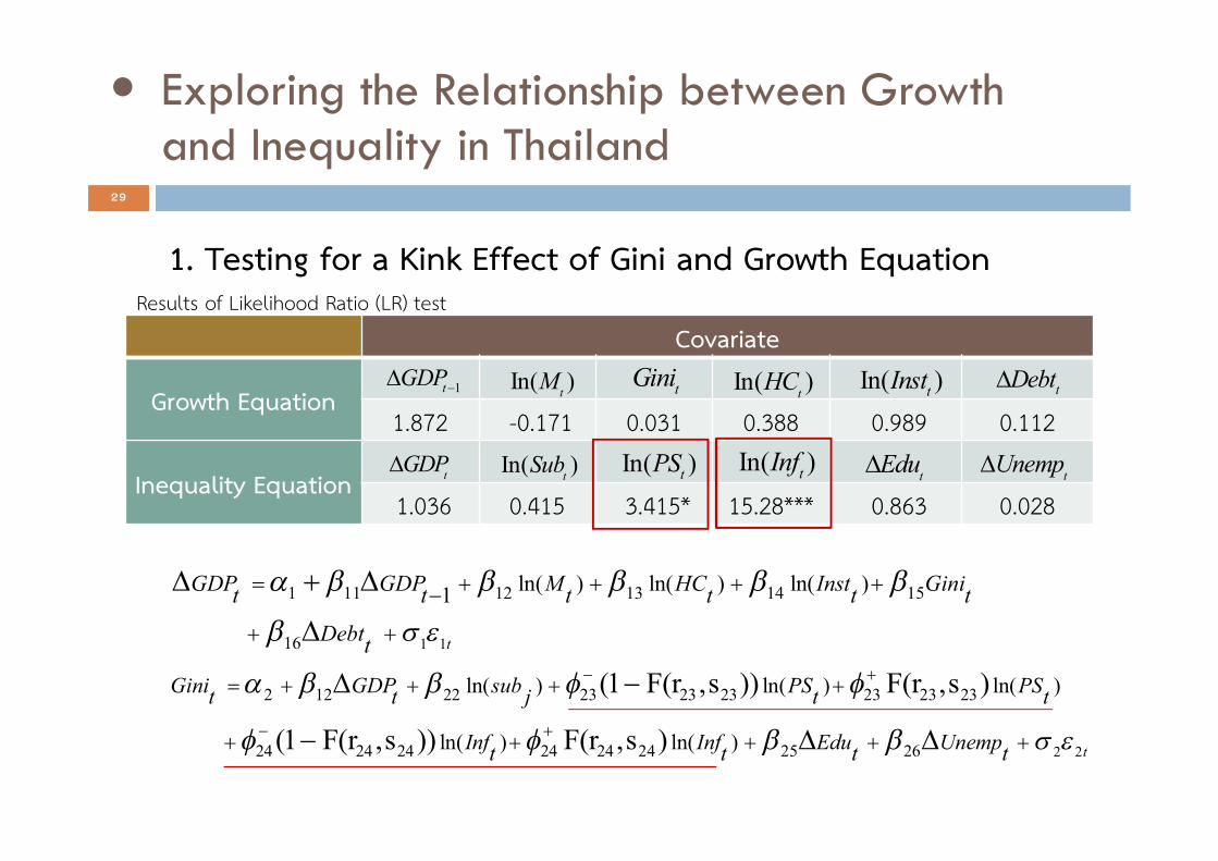
Model Specification22

The model consists of two equations which are modeled simultaneously. The first equation represents the economic growth and the second equation represents income inequality.

GDP growth depends on GDP lagged by one period, monetary base, human capital accumulation, institutional change, Gini coefficient, and government debt.

Income Inequality depends on GDP growth, government subsidy or transfer, share of private sector, inflation, expenditure on education, and rate of unemployed labor.

1 11 12 13 14

15 16 1

ln( ) ln( ) ln( )1GDP GDP M HC Instt t t t t

Gini Debt ut t

2 21 22 23 24

25 26 2

ln(Sub ) ln( ) ln( )Gini GDP PS Inft t t t t

Edu Unemp ut t

23

1 2 4

5

Introduction &Literature Reviews:Motivation of this research

Methodology Model Specification and Variables

Data

3

Simulation Study

6 7

Empirical Results Conclusion

Contents

Data24

We use a quarterly data set of all considered variables, spanning from 1993:Q1 to 2015:Q4.

We apply the Augmented Dickey-Fuller (ADF) unit roots test to the subsets of data to examine whether or not the data series contains a unit root. We found that all variables passed the test at level with probability equal to zero, meaning all of them are stationary.

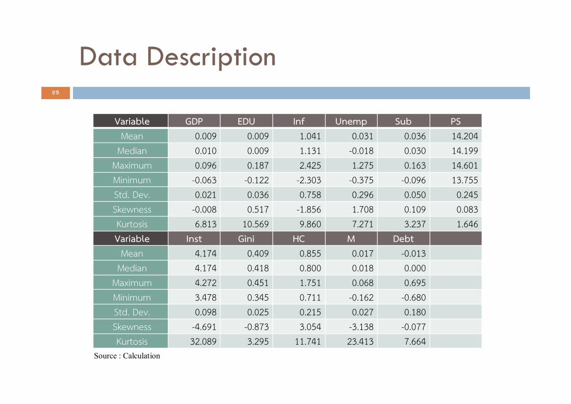
Data Description 25

Variable GDP EDU Inf Unemp Sub PSMean 0.009 0.009 1.041 0.031 0.036 14.204

Median 0.010 0.009 1.131 -0.018 0.030 14.199Maximum 0.096 0.187 2.425 1.275 0.163 14.601Minimum -0.063 -0.122 -2.303 -0.375 -0.096 13.755Std. Dev. 0.021 0.036 0.758 0.296 0.050 0.245Skewness -0.008 0.517 -1.856 1.708 0.109 0.083Kurtosis 6.813 10.569 9.860 7.271 3.237 1.646Variable Inst Gini HC M Debt

Mean 4.174 0.409 0.855 0.017 -0.013Median 4.174 0.418 0.800 0.018 0.000

Maximum 4.272 0.451 1.751 0.068 0.695Minimum 3.478 0.345 0.711 -0.162 -0.680Std. Dev. 0.098 0.025 0.215 0.027 0.180Skewness -4.691 -0.873 3.054 -3.138 -0.077Kurtosis 32.089 3.295 11.741 23.413 7.664

Source : Calculation

26

1 2 4

5

Introduction &Literature Reviews:Motivation of this research

Methodology Model Specification and Variables

Data

3

Simulation Study

6 7

Empirical Results Conclusion

Contents

Empirical Result27

Plotting a simple link between inequality and growth: What is the position of Thailand?

Exploring the Relationship between Growth and Inequality in Thailand

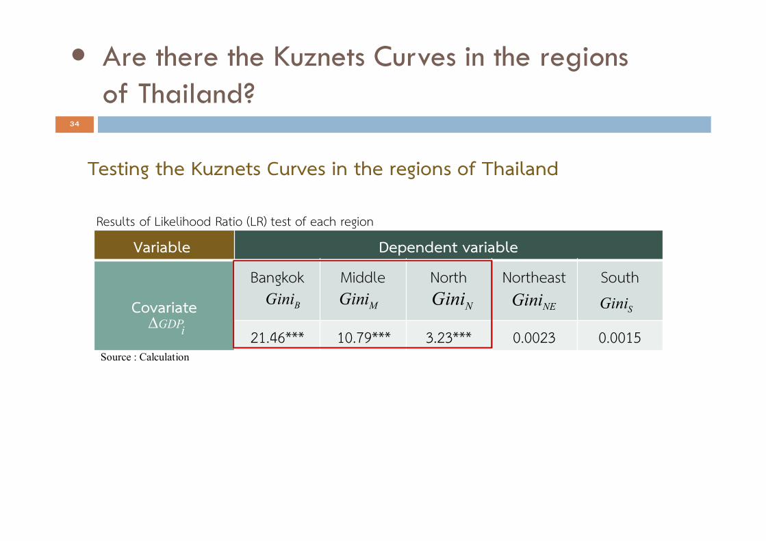
Testing the Kuznets Curves in the regions of Thailand

Policy effect on the economic growth-Gini coefficient

28

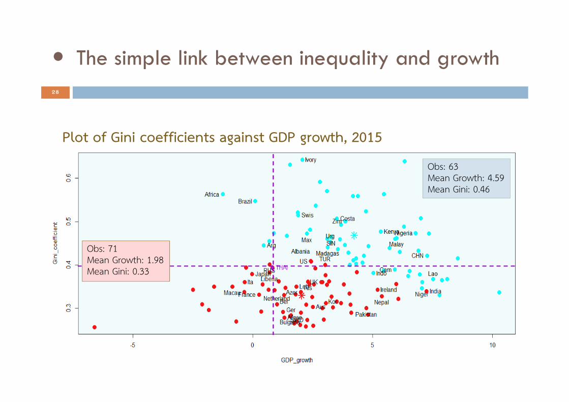
The simple link between inequality and growth

Obs: 71Mean Growth: 1.98Mean Gini: 0.33

Obs: 63Mean Growth: 4.59Mean Gini: 0.46

Plot of Gini coefficients against GDP growth, 2015

29

1. Testing for a Kink Effect of Gini and Growth Equation

Exploring the Relationship between Growth and Inequality in Thailand

Covariate

Growth Equation1.872 -0.171 0.031 0.388 0.989 0.112

Inequality Equation1.036 0.415 3.415* 15.28*** 0.863 0.028

1tGDP In( )tM tGini In( )tHC In( )tInst tDebt

tGDP In( )tSub In( )tPS In( )tInftEdu tUnemp

1 1

1 11 12 13 14 15

16

ln( ) ln( ) ln( )1

t

GDP GDP M HC Inst Ginit t t t t t

Debtt

2 2

2 12 22 23 23 23 23 23 23

24 24 24 24 24 24 25 26

ln( ) ln( ) ln( )

ln( ) ln( )

(1 F(r ,s )) F(r ,s )

(1 F(r ,s )) F(r ,s ) t

Gini GDP sub PS PSt t j t t

Inf Inf Edu Unempt t t t

Results of Likelihood Ratio (LR) test

30

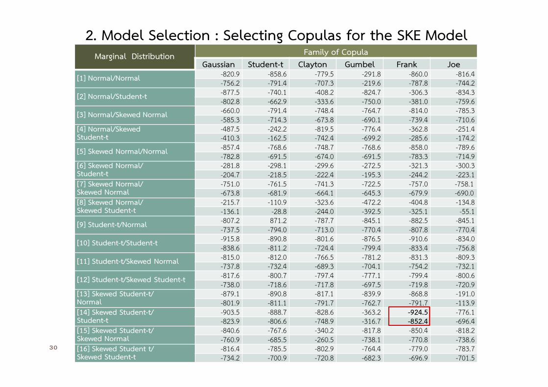
Marginal Distribution Family of CopulaGaussian Student-t Clayton Gumbel Frank Joe

[1] Normal/Normal -820.9 -858.6 -779.5 -291.8 -860.0 -816.4-756.2 -791.4 -707.3 -219.6 -787.8 -744.2

[2] Normal/Student-t -877.5 -740.1 -408.2 -824.7 -306.3 -834.3-802.8 -662.9 -333.6 -750.0 -381.0 -759.6

[3] Normal/Skewed Normal -660.0 -791.4 -748.4 -764.7 -814.0 -785.3-585.3 -714.3 -673.8 -690.1 -739.4 -710.6

[4] Normal/Skewed Student-t

-487.5 -242.2 -819.5 -776.4 -362.8 -251.4-410.3 -162.5 -742.4 -699.2 -285.6 -174.2

[5] Skewed Normal/Normal -857.4 -768.6 -748.7 -768.6 -858.0 -789.6-782.8 -691.5 -674.0 -691.5 -783.3 -714.9

[6] Skewed Normal/Student-t

-281.8 -298.1 -299.6 -272.5 -321.3 -300.3-204.7 -218.5 -222.4 -195.3 -244.2 -223.1

[7] Skewed Normal/Skewed Normal

-751.0 -761.5 -741.3 -722.5 -757.0 -758.1-673.8 -681.9 -664.1 -645.3 -679.9 -690.0

[8] Skewed Normal/Skewed Student-t

-215.7 -110.9 -323.6 -472.2 -404.8 -134.8-136.1 -28.8 -244.0 -392.5 -325.1 -55.1

[9] Student-t/Normal -807.2 871.2 -787.7 -845.1 -882.5 -845.1-737.5 -794.0 -713.0 -770.4 -807.8 -770.4

[10] Student-t/Student-t -915.8 -890.8 -801.6 -876.5 -910.6 -834.0-838.6 -811.2 -724.4 -799.4 -833.4 -756.8

[11] Student-t/Skewed Normal -815.0 -812.0 -766.5 -781.2 -831.3 -809.3-737.8 -732.4 -689.3 -704.1 -754.2 -732.1

[12] Student-t/Skewed Student-t -817.6 -800.7 -797.4 -777.1 -799.4 -800.6-738.0 -718.6 -717.8 -697.5 -719.8 -720.9

[13] Skewed Student-t/Normal

-879.1 -890.8 -817.1 -839.9 -868.8 -191.0-801.9 -811.1 -791.7 -762.7 -791.7 -113.9

[14] Skewed Student-t/Student-t

-903.5 -888.7 -828.6 -363.2 -924.5 -776.1-823.9 -806.6 -748.9 -316.7 -852.4 -696.4

[15] Skewed Student-t/Skewed Normal

-840.6 -767.6 -340.2 -817.8 -850.4 -818.2-760.9 -685.5 -260.5 -738.1 -770.8 -738.6

[16] Skewed Student t/Skewed Student-t

-816.4 -785.5 -802.9 -764.4 -779.0 -783.7-734.2 -700.9 -720.8 -682.3 -696.9 -701.5

2. Model Selection : Selecting Copulas for the SKE Model

31

Variables Estimated Value S.E. ( )Intercept term 0.0359* 2.16GDP growth lagged by one period 0.0596 6.72Monetary base 0.0384 2.62Human Capital Accumulation 0.0119 0.93Institution -0.0166*** 0.11Gini Coefficient 0.0225** 0.95Government debt 0.0638* 3.97Sigma ( ) 0.0355** 1.97Degree of freedom Student-t 2.4739*** 50.83Degree of freedom Skewed Student-t 0.5666*** 19.71

1

210

3. Estimation results of Copula based SKE model

The estimates of the growth equation

Note: Growth and inequality equations are estimated simultaneously but we need to show the result separately due to a page limitation.

32

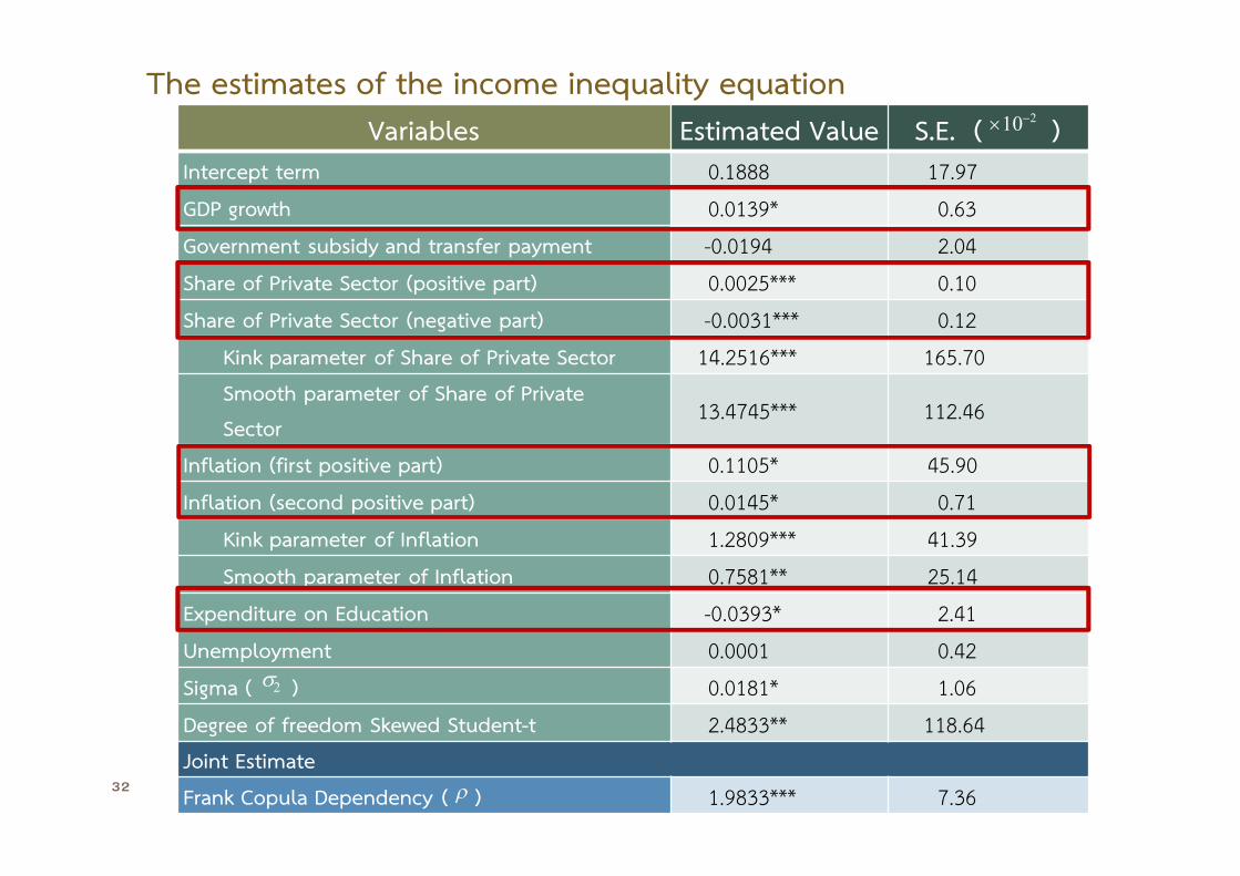
Variables Estimated Value S.E. ( )Intercept term 0.1888 17.97GDP growth 0.0139* 0.63Government subsidy and transfer payment -0.0194 2.04Share of Private Sector (positive part) 0.0025*** 0.10Share of Private Sector (negative part) -0.0031*** 0.12

Kink parameter of Share of Private Sector 14.2516*** 165.70Smooth parameter of Share of Private

Sector13.4745*** 112.46

Inflation (first positive part) 0.1105* 45.90Inflation (second positive part) 0.0145* 0.71

Kink parameter of Inflation 1.2809*** 41.39Smooth parameter of Inflation 0.7581** 25.14

Expenditure on Education -0.0393* 2.41Unemployment 0.0001 0.42Sigma ( ) 0.0181* 1.06Degree of freedom Skewed Student-t 2.4833** 118.64Joint Estimate

Frank Copula Dependency ( ) 1.9833*** 7.36

2

210

The estimates of the income inequality equation

33

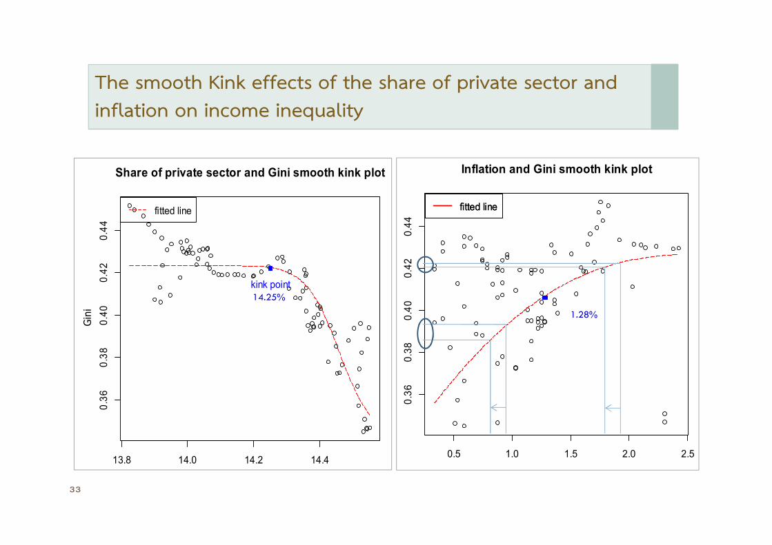
The smooth Kink effects of the share of private sector and inflation on income inequality

13.8 14.0 14.2 14.4

0.36

0.38

0.40

0.42

0.44

Share of private sector and Gini smooth kink plot

fitted line

kink point

0.5 1.0 1.5 2.0 2.5

0.36

0.38

0.40

0.42

0.44

Inflation and Gini smooth kink plot

fitted linefitted line

Gini

14.25%

1.28%

34

Source : Calculation

Variable Dependent variable

Covariate

Bangkok Middle North Northeast South

21.46*** 10.79*** 3.23*** 0.0023 0.0015

BGini MGini NGini NEGiniSGini

GDPi

Results of Likelihood Ratio (LR) test of each region

Are there the Kuznets Curves in the regions of Thailand?

Testing the Kuznets Curves in the regions of Thailand

35

2

210

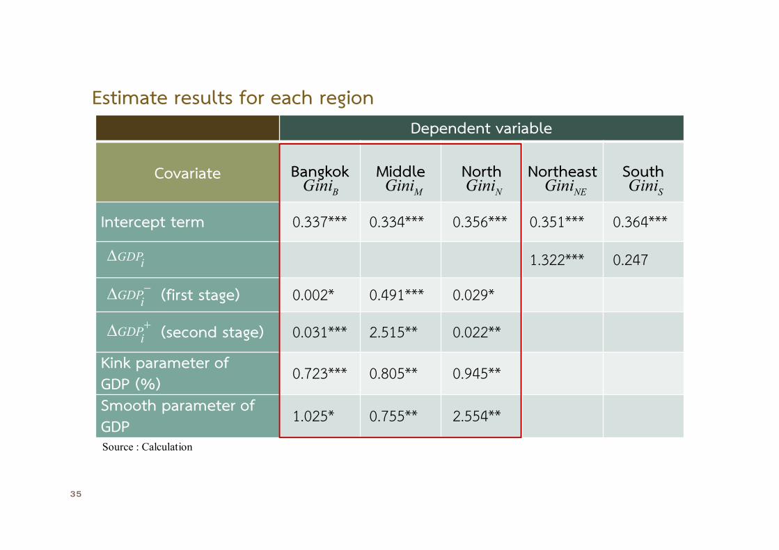
Estimate results for each region

Dependent variable

Covariate Bangkok Middle North Northeast South

Intercept term 0.337*** 0.334*** 0.356*** 0.351*** 0.364***

1.322*** 0.247

(first stage) 0.002* 0.491*** 0.029*

(second stage) 0.031*** 2.515** 0.022**

Kink parameter of GDP (%)

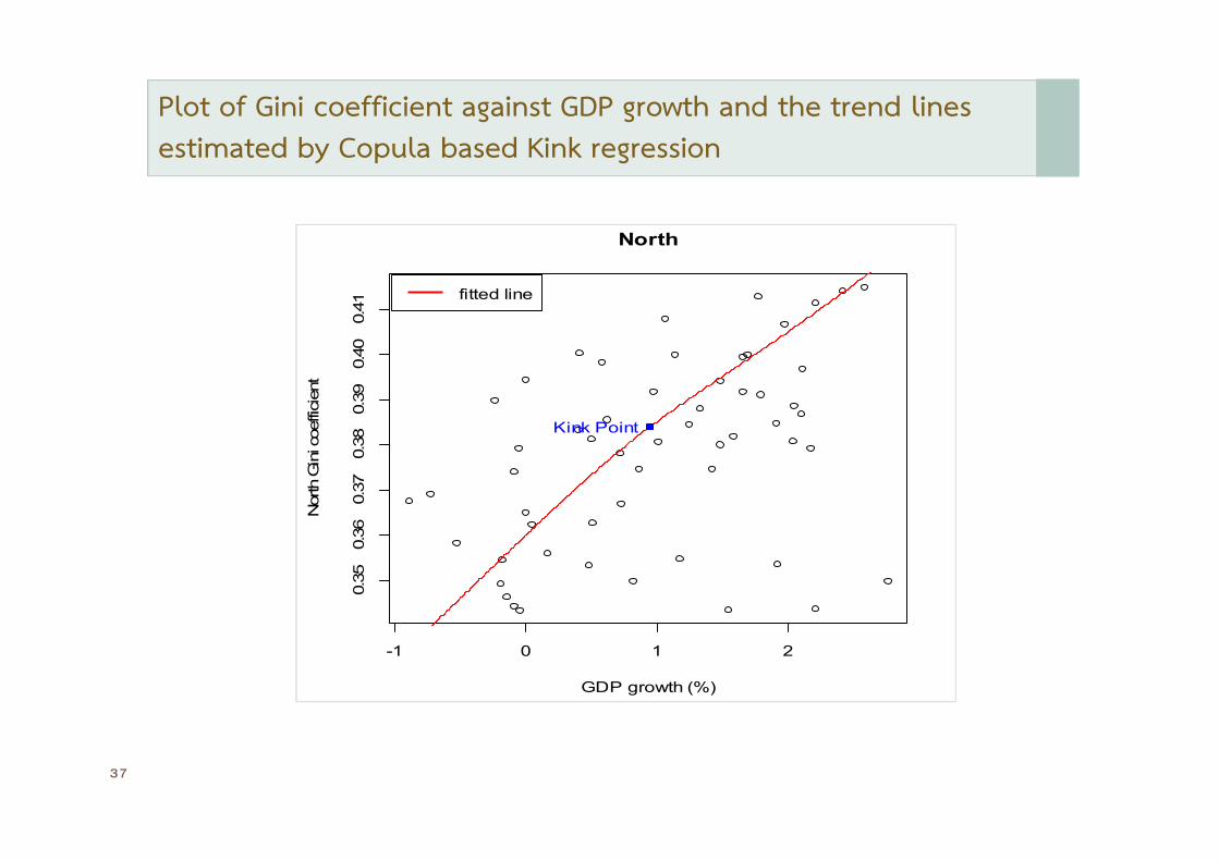
0.723*** 0.805** 0.945**

Smooth parameter of GDP

1.025* 0.755** 2.554**

GDPi

GDPi

GDPi

BGini MGini NGini NEGini SGini

Source : Calculation

36

Plot of Gini coefficient against GDP growth and the trend lines estimated by Copula based Kink regression

-2 -1 0 1 2

0.32

0.34

0.36

0.38

0.40

Bangkok

GDP growth (%)

Ban

gkok

Gin

i coe

ffici

ent

Kink Point

fitted line

-2 -1 0 1 2 3

0.33

0.34

0.35

0.36

0.37

Center

GDP growth (%)

Cen

ter G

ini c

oeffi

cien

t

Kink Point

fitted line

37

Plot of Gini coefficient against GDP growth and the trend lines estimated by Copula based Kink regression

-1 0 1 2

0.35

0.36

0.37

0.38

0.39

0.40

0.41

North

GDP growth (%)

Nor

th G

ini c

oeffi

cien

t

Kink Point

fitted line

38

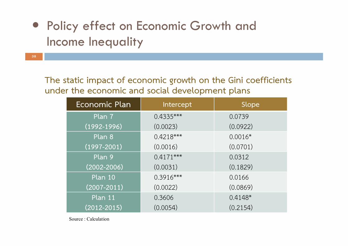
Policy effect on Economic Growth and Income Inequality

The static impact of economic growth on the Gini coefficients under the economic and social development plans

Source : Calculation

Economic Plan Intercept Slope

Plan 7 (1992-1996)

0.4335***(0.0023)

0.0739(0.0922)

Plan 8 (1997-2001)

0.4218***(0.0016)

0.0016*(0.0701)

Plan 9(2002-2006)

0.4171***(0.0031)

0.0312(0.1829)

Plan 10(2007-2011)

0.3916***(0.0022)

0.0166(0.0869)

Plan 11 (2012-2015)

0.3606(0.0054)

0.4148*(0.2154)

39

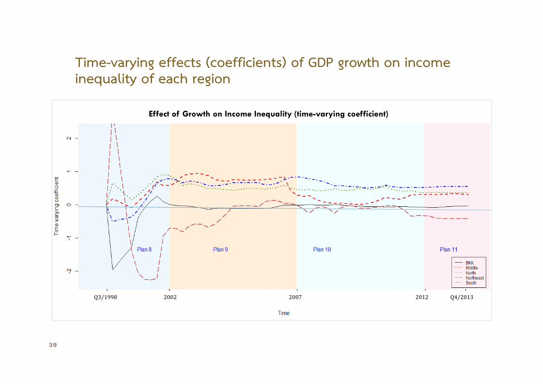
Time-varying effects (coefficients) of GDP growth on income inequality of each region

Q3/1998 2002 2007 2012 Q4/2013

Effect of Growth on Income Inequality (time-varying coefficient)

40

1 2 4

5

Introduction &Literature Reviews:Motivation of this research

Methodology Model Specification and Variables

Data

3

Simulation Study

6 7

Empirical Results Conclusion

Contents

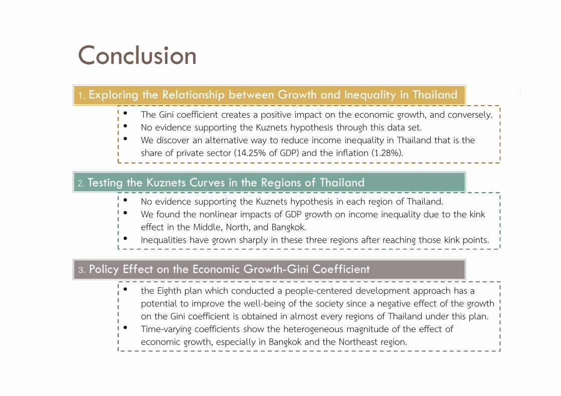
Conclusion1. Exploring the Relationship between Growth and Inequality in Thailand

2. Testing the Kuznets Curves in the Regions of Thailand

3. Policy Effect on the Economic Growth-Gini Coefficient

• The Gini coefficient creates a positive impact on the economic growth, and conversely.• No evidence supporting the Kuznets hypothesis through this data set. • We discover an alternative way to reduce income inequality in Thailand that is the

share of private sector (14.25% of GDP) and the inflation (1.28%).

• No evidence supporting the Kuznets hypothesis in each region of Thailand.• We found the nonlinear impacts of GDP growth on income inequality due to the kink

effect in the Middle, North, and Bangkok.• Inequalities have grown sharply in these three regions after reaching those kink points.

• the Eighth plan which conducted a people-centered development approach has a potential to improve the well-being of the society since a negative effect of the growth on the Gini coefficient is obtained in almost every regions of Thailand under this plan.

• Time-varying coefficients show the heterogeneous magnitude of the effect of economic growth, especially in Bangkok and the Northeast region.

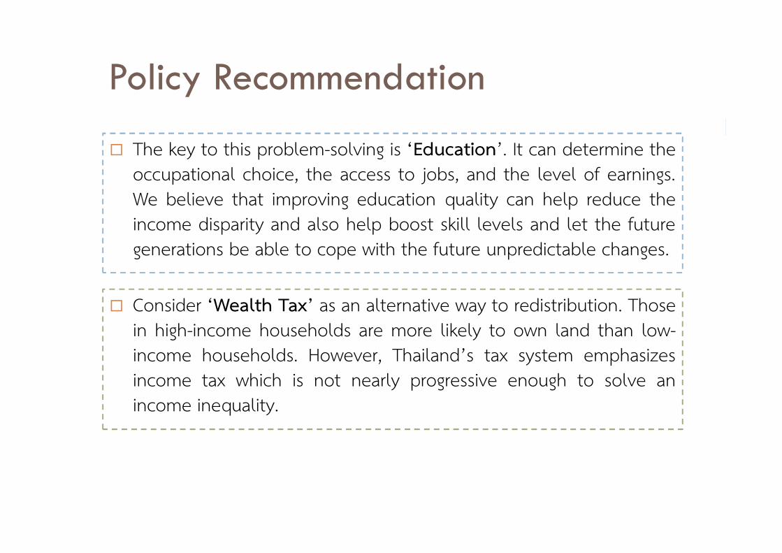
Policy Recommendation42

The key to this problem-solving is ‘Education’. It can determine the occupational choice, the access to jobs, and the level of earnings. We believe that improving education quality can help reduce the income disparity and also help boost skill levels and let the future generations be able to cope with the future unpredictable changes.

Consider ‘Wealth Tax’ as an alternative way to redistribution. Those in high-income households are more likely to own land than low-income households. However, Thailand’s tax system emphasizes income tax which is not nearly progressive enough to solve an income inequality.

ขอบคณุค่ะ43