AnalyzingandDeveloping Role-BasedAccessControlModels · AnalyzingandDeveloping...

Analyzing and Developing

Role-Based Access Control Models

by

Liang Chen

A thesis submitted in fulfilment of the requirements for the Degree of

Doctor of Philosophy

in the

University of London

Information Security Group

Department of Mathematics

Royal Holloway, University of London

2011

Declaration

These doctoral studies were conducted under the supervision of Dr Jason Crampton.

The work presented in this thesis is the result of original research carried out by

myself, in collaboration with others, whilst enrolled in the Department of Mathemat-

ics, Royal Holloway, University of London as a candidate for the degree of Doctor of

Philosophy. This work has not been submitted for any other degree or award in any

other university or educational establishment.

Liang Chen

November, 2010

2

Abstract

Role-based access control (RBAC) has become today’s dominant access control model,

and many of its theoretical and practical aspects are well understood. However, certain

aspects of more advanced RBAC models, such as the relationship between permission

usage and role activation and the interaction between inheritance and constraints, re-

main poorly understood. Moreover, the computational complexity of some important

problems in RBAC remains unknown. In this thesis we consider these issues, develop

new RBAC models and answer a number of these questions.

We develop an extended RBAC model that proposes an alternative way to dis-

tinguish between activation and usage hierarchies. Our extended RBAC model has

well-defined semantics, derived from a graph-based interpretation of RBAC state.

Pervasive computing environments have created a requirement for access control

systems in which authorization is dependent on spatio-temporal constraints. We de-

velop a family of simple, expressive and flexible spatio-temporal RBAC models, and

extend these models to include activation and usage hierarchies. Unlike existing work,

our models address the interaction between spatio-temporal constraints and inheritance

in RBAC, and are consistent and compatible with the ANSI RBAC standard.

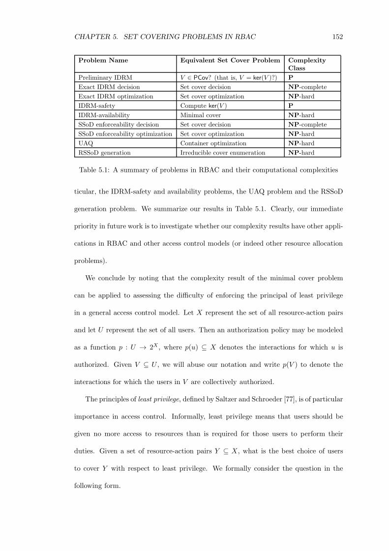
A number of interesting problems have been defined and studied in the context

of RBAC recently. We explore some variations on the set cover problem and use

these variations to establish the computational complexity of these problems. Most

importantly, we prove that the minimal cover problem – a generalization of the set

cover problem – is NP-hard. The minimal cover problem is then used to determine the

complexity of the inter-domain role mapping problem and the user authorization query

problem in RBAC. We also design a number of efficient heuristic algorithms to answer

the minimal cover problem, and conduct experiments to evaluate the quality of these

algorithms.

3

Contents

Abstract 3

Contents 4

List of Figures 7

List of Tables 8

Acknowledgements 9

1 Introduction 11

1.1 Motivation . . . . . . . . . . . . . . . . . . . . . . . . . . . . . . . . . . 15

1.1.1 The role hierarchy and inheritance . . . . . . . . . . . . . . . . . 15

1.1.2 Extended RBAC . . . . . . . . . . . . . . . . . . . . . . . . . . . 17

1.1.3 Spatio-temporal RBAC . . . . . . . . . . . . . . . . . . . . . . . 18

1.1.4 Computational problems in RBAC . . . . . . . . . . . . . . . . . 19

1.2 Contributions . . . . . . . . . . . . . . . . . . . . . . . . . . . . . . . . . 20

1.3 Structure of the thesis . . . . . . . . . . . . . . . . . . . . . . . . . . . . 22

1.4 Publications . . . . . . . . . . . . . . . . . . . . . . . . . . . . . . . . . . 24

2 Background 26

2.1 Access control . . . . . . . . . . . . . . . . . . . . . . . . . . . . . . . . . 26

2.1.1 Discretionary access control . . . . . . . . . . . . . . . . . . . . . 30

2.1.2 Mandatory access control . . . . . . . . . . . . . . . . . . . . . . 32

2.2 Role-based access control . . . . . . . . . . . . . . . . . . . . . . . . . . 34

2.2.1 RBAC96 . . . . . . . . . . . . . . . . . . . . . . . . . . . . . . . 36

2.2.2 ANSI-RBAC . . . . . . . . . . . . . . . . . . . . . . . . . . . . . 40

2.3 Complexity theory . . . . . . . . . . . . . . . . . . . . . . . . . . . . . . 43

4

3 The OP-RBAC Model and its Applications 49

3.1 The OP-RBAC model . . . . . . . . . . . . . . . . . . . . . . . . . . . . 51

3.2 The Bell-LaPadula model and extensions . . . . . . . . . . . . . . . . . 52

3.3 Implementing BLP using OP-RBAC . . . . . . . . . . . . . . . . . . . . 54

3.3.1 Security labels . . . . . . . . . . . . . . . . . . . . . . . . . . . . 55

3.3.2 BLP0 . . . . . . . . . . . . . . . . . . . . . . . . . . . . . . . . . 57

3.3.3 BLP1 . . . . . . . . . . . . . . . . . . . . . . . . . . . . . . . . . 60

3.3.4 BLP2 . . . . . . . . . . . . . . . . . . . . . . . . . . . . . . . . . 60

3.3.5 BLP3 . . . . . . . . . . . . . . . . . . . . . . . . . . . . . . . . . 63

3.3.6 BLP4 . . . . . . . . . . . . . . . . . . . . . . . . . . . . . . . . . 65

3.3.7 The discretionary security property . . . . . . . . . . . . . . . . . 68

3.3.8 Discussion . . . . . . . . . . . . . . . . . . . . . . . . . . . . . . . 69

3.4 Other applications . . . . . . . . . . . . . . . . . . . . . . . . . . . . . . 72

3.4.1 Separation of duty . . . . . . . . . . . . . . . . . . . . . . . . . . 72

3.4.2 Usage and activation hierarchies . . . . . . . . . . . . . . . . . . 75

3.5 Conclusion . . . . . . . . . . . . . . . . . . . . . . . . . . . . . . . . . . 80

4 Spatio-Temporal RBAC 82

4.1 Graph-based formulation of RBAC1 . . . . . . . . . . . . . . . . . . . . 86

4.2 ERBAC07 . . . . . . . . . . . . . . . . . . . . . . . . . . . . . . . . . . . 87

4.2.1 Syntax . . . . . . . . . . . . . . . . . . . . . . . . . . . . . . . . . 87

4.2.2 Semantics . . . . . . . . . . . . . . . . . . . . . . . . . . . . . . . 89

4.2.3 ERBAC96, GTRBAC and ERBAC07 . . . . . . . . . . . . . . . 91

4.3 Spatio-temporal RBAC . . . . . . . . . . . . . . . . . . . . . . . . . . . 93

4.3.1 RBAC=ST : the standard model . . . . . . . . . . . . . . . . . . . 93

4.3.2 RBAC+ST : the strong model . . . . . . . . . . . . . . . . . . . . . 95

4.3.3 RBAC−ST : the weak model . . . . . . . . . . . . . . . . . . . . . . 97

4.3.4 Trusted entities . . . . . . . . . . . . . . . . . . . . . . . . . . . . 98

4.3.5 A note on RBAC1-style syntax . . . . . . . . . . . . . . . . . . . 100

4.3.6 Integration with ANSI-RBAC . . . . . . . . . . . . . . . . . . . . 100

4.4 Spatio-temporal ERBAC . . . . . . . . . . . . . . . . . . . . . . . . . . . 101

4.4.1 ERBAC=ST : the standard model . . . . . . . . . . . . . . . . . . . 102

4.4.2 ERBAC+ST : the strong model . . . . . . . . . . . . . . . . . . . . 102

4.4.3 ERBAC−ST : the weak model . . . . . . . . . . . . . . . . . . . . . 103

4.5 Practical considerations in spatio-temporal RBAC . . . . . . . . . . . . 103

5

4.5.1 Partial transitive closure . . . . . . . . . . . . . . . . . . . . . . . 103

4.5.2 Full transitive closure . . . . . . . . . . . . . . . . . . . . . . . . 107

4.5.3 Is the use of hierarchies realistic? . . . . . . . . . . . . . . . . . . 108

4.5.4 Concluding remarks . . . . . . . . . . . . . . . . . . . . . . . . . 114

4.6 Spatio-temporal domains . . . . . . . . . . . . . . . . . . . . . . . . . . 115

4.6.1 Representing location . . . . . . . . . . . . . . . . . . . . . . . . 116

4.6.2 Representing time . . . . . . . . . . . . . . . . . . . . . . . . . . 117

4.6.3 Example . . . . . . . . . . . . . . . . . . . . . . . . . . . . . . . . 117

4.7 Related work . . . . . . . . . . . . . . . . . . . . . . . . . . . . . . . . . 121

4.7.1 Temporal constraints in GTRBAC . . . . . . . . . . . . . . . . . 122

4.7.2 Spatio-temporal RBAC . . . . . . . . . . . . . . . . . . . . . . . 124

4.7.3 Summary . . . . . . . . . . . . . . . . . . . . . . . . . . . . . . . 125

4.8 Conclusion . . . . . . . . . . . . . . . . . . . . . . . . . . . . . . . . . . 125

5 Set Covering Problems in RBAC 128

5.1 The set cover problem . . . . . . . . . . . . . . . . . . . . . . . . . . . . 131

5.2 Variations on the set cover problem . . . . . . . . . . . . . . . . . . . . . 132

5.2.1 The kernel and shell . . . . . . . . . . . . . . . . . . . . . . . . . 133

5.2.2 Minimality, optimality and irreducibility . . . . . . . . . . . . . . 135

5.2.3 The minimal cover problem . . . . . . . . . . . . . . . . . . . . . 137

5.2.4 The irreducible cover problem . . . . . . . . . . . . . . . . . . . . 141

5.3 Covering problems in RBAC . . . . . . . . . . . . . . . . . . . . . . . . 142

5.3.1 The inter-domain role mapping problem . . . . . . . . . . . . . . 143

5.3.2 The user authorization query problem . . . . . . . . . . . . . . . 146

5.3.3 Separation of duty . . . . . . . . . . . . . . . . . . . . . . . . . . 149

5.4 Conclusion . . . . . . . . . . . . . . . . . . . . . . . . . . . . . . . . . . 151

6 Heuristic Algorithms 154

6.1 The weighted set cover optimization problem . . . . . . . . . . . . . . . 155

6.2 Designing heuristic algorithms . . . . . . . . . . . . . . . . . . . . . . . . 157

6.2.1 Designing an algorithm . . . . . . . . . . . . . . . . . . . . . . . 157

6.2.2 Evaluation metrics . . . . . . . . . . . . . . . . . . . . . . . . . . 159

6.3 Evaluating heuristic algorithms . . . . . . . . . . . . . . . . . . . . . . . 160

6.3.1 Data generation . . . . . . . . . . . . . . . . . . . . . . . . . . . 161

6.3.2 Scoring functions . . . . . . . . . . . . . . . . . . . . . . . . . . . 162

6

6.3.3 Results . . . . . . . . . . . . . . . . . . . . . . . . . . . . . . . . 164

6.3.4 A hybrid algorithm . . . . . . . . . . . . . . . . . . . . . . . . . . 166

6.4 Concluding remarks . . . . . . . . . . . . . . . . . . . . . . . . . . . . . 170

7 Conclusions and Future Work 172

7.1 Summary of contributions . . . . . . . . . . . . . . . . . . . . . . . . . . 172

7.2 Future work . . . . . . . . . . . . . . . . . . . . . . . . . . . . . . . . . . 176

References 180

7

List of Figures

2.1 The generic architecture of an access control mechanism . . . . . . . . . 30

2.2 A simple relationship between users, roles and permissions . . . . . . . . 36

2.3 The RBAC96 family of models . . . . . . . . . . . . . . . . . . . . . . . 37

3.1 A role hierarchy and the associated lattice . . . . . . . . . . . . . . . . . 56

3.2 A read hierarchy and the corresponding append hierarchy . . . . . . . . 71

3.3 Implementing separation of duty using different types of permissions . . 74

3.4 ERBAC96 activation and usage hierarchies . . . . . . . . . . . . . . . . 76

3.5 Transforming ERBAC96 into OP-RBAC . . . . . . . . . . . . . . . . . . 77

3.6 Transforming the ERBAC96 permission set and PA relation . . . . . . . 78

4.1 A graphical representation of ERBAC07 states . . . . . . . . . . . . . . 89

4.2 Decomposing a GTRBAC hierarchy into ERBAC07 hierarchies . . . . . 92

4.3 RBAC1 configurations and their effect on spatio-temporal configurations 95

4.4 A comparison of spatio-temporal models for encoding constraints . . . . 112

4.5 An example of an RBAC1 configuration . . . . . . . . . . . . . . . . . . 118

4.6 An example of the specification of spatio-temporal domains . . . . . . . 119

4.7 An example of ERBAC07 activation and usage hierarchies . . . . . . . . 121

5.1 A graphical representation of X and C, and a Hasse diagram of PCov . . 134

5.2 The IRR-Gen algorithm . . . . . . . . . . . . . . . . . . . . . . . . . . . 137

5.3 Correspondence between the set cover and container problems . . . . . . 140

6.1 A graphical representation of the minimal cover problem instances . . . 167

8

List of Tables

1.1 Contributions of the thesis . . . . . . . . . . . . . . . . . . . . . . . . . . 23

2.1 An access control matrix . . . . . . . . . . . . . . . . . . . . . . . . . . . 31

2.2 ANSI-RBAC mapping functions . . . . . . . . . . . . . . . . . . . . . . . 41

3.1 A summary of the different Bell-LaPadula models . . . . . . . . . . . . . 53

3.2 BLP4 . . . . . . . . . . . . . . . . . . . . . . . . . . . . . . . . . . . . . 66

4.1 Spatio-temporal ANSI-RBAC mapping functions . . . . . . . . . . . . . 101

5.1 A summary of problems in RBAC and their computational complexities 152

6.1 The results of the best heuristic algorithms for different |V | . . . . . . . 165

6.2 The results for dynamic heuristic algorithms when |V | = 5 . . . . . . . . 166

6.3 The results for alg211, alg311 and alg411 . . . . . . . . . . . . . . . . . . 169

9

Acknowledgements

Firstly, I would like to express my gratitude to my supervisor, Dr Jason Crampton, for

giving me the opportunity to study for a PhD. His excellent guidance, critical feedback

and active involvement have made a huge contribution to the quality and presentation

of my work. I also thank Jason for his endless patience and constant encouragement

whenever I was in doubt in the last years. The experience to work with Jason has been

invaluable, and this experience will be most useful and important for my future.

I am grateful to my advisor, Professor Chris Mitchell, for his constructive comments

on my work in the annual review meetings. I am also thankful to Chris for granting me

a College Research Studentship, which was extremely helpful in alleviating the financial

burden of my PhD studies.

I owe a great debt to colleagues within the Information Security Group, Royal Hol-

loway College: Dr Jiqiang Lu, Dr Hoon Wei Lim, Dr Geong Sen Poh, Chunhua Chen,

and Ziyad Al-Salloum for their inspiring discussions of PhD research, and generally be-

ing great office mates. In particular, I would like to thank Hemanth Khambhammettu

for the many stimulating conversions we have had, and for the time he spent reading

and commenting on the chapters of the thesis. I also would like to thank Dr Charles

Morisset for proof reading of chapters of the thesis despite his busy schedule.

During my stay in England, I have made many new friends in the last few years but

two of these in particular are considered to be my closest and best friends: Yichuan

Chen and Robert Williams. I feel very fortunate to have met Yichuan as I can share

my most inner thoughts with him, and he has been of great help to me in so many

different ways. I am also very grateful to Robert for his generous help and kindness

with any problems I have encountered in my everyday life.

Finally, I would like to thank my parents for their continuous support and encour-

agement. I am especially indebted to my fiancee, Zheng Ning, for her unconditional

love and support, who also makes my life better and complete in the last three years.

10

Chapter 1

Introduction

The protection of information in multi-user computer systems has become increas-

ingly important as a result of the rapid development and widespread deployment of

computer systems in our daily life. The most common protection measures used in

computer system are prevention, detection and recovery [46]. Prevention is applied to

prevent information from being damaged. In other words, its purpose is to prevent all

unauthorized access to information. Detection allows us to detect when information has

been damaged, how it has been damaged, and who has caused the damage. Recovery

allows us to restore the information that has been damaged or to assess and repair any

damage to the information. In this thesis, we are only concerned with prevention.

The prevention measure is regarded as the traditional core of computer security,

which usually attempts to achieve three security goals: confidentiality, integrity and

availability. These security goals are concerned with prevention of unauthorized dis-

closure of information, unauthorized modification of information, and unauthorized

withholding of information, respectively [26]. In this thesis, we focus on studying ac-

cess control, one of the most important prevention techniques in computer systems. In

particular, it can help enforce confidentiality and integrity, and can also provide a basis

11

CHAPTER 1. INTRODUCTION 12

for availability. For example, an attacker who gains unauthorized access to a sensitive

document is likely to have little trouble making this document unavailable to valid and

authorized users. Generally speaking, access control is concerned with limiting access

by users to protected resources. In multi-user computer systems, some resources may

be publicly accessible by all users, some may only be accessible by a restricted audience,

and some may be private to the user who creates those resources. These requirements

are usually expressed by access control policies that generally specify who is allowed to

access which resources in a computer system. Access control mechanisms are used to

implement access control policies, and ensure that users’ requests to access resources

are only granted if those requests are authorized by the policies.

Access control has been the subject of considerable research and developments over

the last 30 years. The Trusted Computer System Evaluation Criteria (TCSEC), com-

monly known as the “Orange Book” [89], defines two different types of access control:

discretionary access control and mandatory access control. Discretionary access con-

trol restricts access to resources based on the identity of users. The two key features of

discretionary access control is that each resource is required to have an owner, and the

owner is able to control who can access the resources she owns. Discretionary access

control is the most widely used form of access control being used in operating systems

such as UNIX and Windows NT. Operating systems usually implement discretionary

access control on the basis of access control lists. That is, each resource in the system

is associated with a list of users who are entitled to access that resource. A request

from a user to access a given resource is granted if the user is in the access control list.

Mandatory access control constrains the interactions of users with resources on

the basis of security attributes associated with users and resources. A request from

a user to access a resource is granted if certain inequalities comparing the security

attributes of the user and the resource are satisfied. Unlike discretionary access control,


changes to the authorization policies in mandatory access control are controlled by a

higher authority, rather than individual users. In other words, system administrators

define mandatory access control policies that can be centrally enforced for all users.

The Bell-LaPadula model [12] is probably the most widely known security model and

incorporates a mandatory information flow policy for confidentiality [35]. Informally,

the mandatory information flow policy comprises the simple security property and the

*-property. The simple security property requires that a user is only allowed to read

a resource if the security attribute of the user is at least as high as that of resource

being read. Conversely, the *-property requires that a user is only allowed to write

to a resource if the security attribute of the resource is at least as high as that of the

user. These kinds of mandatory access control policies are commonly used in military

applications and commercially sensitive applications.

However, modern business information systems typically comprise millions of re-

sources and thousands of users. The complexity of such systems makes it difficult to

employ discretionary access control that might require the management of millions of

access control lists or other similar access control data structures. Conversely, manda-

tory access control has been found to be too restrictive for general organizational in-

formation systems [39].

Role-based access control (RBAC) [40, 70, 83] has emerged as the primary alter-

native to discretionary access control and mandatory access control, because of its

potential to reduce the complexity and cost of access control administration in organi-

zational systems. The basic idea of RBAC is to introduce the concept of a role, which

acts as a “bridge” between users and permissions1. A user can use a permission by

activating a role to which the user and the permission are assigned. This approach

1Informally, the term permission refers to some combination of resource and action that usersattempts to perform.


of associating users and permissions with roles greatly simplifies the management of

permissions for which a user is authorized. For example, if an employee is required to

change his position within an organization, we simply assign a new set of roles to this

user without having to directly assign a completely new set of permissions to him.

RBAC further reduces the administrative burden by introducing the idea of a role

hierarchy. The role hierarchy generally supports two different types of inheritance:

permissions are inherited upwards and the set of roles available to a user is aggregated

downwards. For example, if role r is senior to r′ in the role hierarchy, then any permis-

sion assigned to r′ is implicitly assigned to r, and any user assigned to r can activate r′.

These two types of inheritance are called permission usage and role activation respec-

tively. In other words, a role hierarchy can be used to reduce the number of explicit

assignments in the user-role and permission-role relations.

The fundamental concepts of RBAC are now well established and are detailed in the

recent release of the ANSI RBAC standard [2]. RBAC has also been incorporated into

several commercial software products offered by major information technology vendors,

such as Authorization Manager in Windows Server 2003, Oracle Access Manager, IBM

Tivoli Policy Manager [59] and SAM Jupiter [6]. Although RBAC has obtained consid-

erable maturity in many theoretical and practical aspects, the uses of role hierarchies

in RBAC has a number of inconvenient consequences which have not been thoroughly

addressed. In addition, certain aspects of more advanced RBAC models, such as the

relationship between permissions usage and role activation and the interaction between

inheritance and constraints, remain poorly understood. Moreover, the computational

complexity of some important problems in RBAC remains unknown. The main goal of

this thesis is to examine issues noted above, to develop new RBAC models for address-

ing some of these issues, and to analyze and answer a number of outstanding problems

in RBAC.


1.1 Motivation

At the most general level, this thesis is concerned with role hierarchies and the way

in which they interact with other parts of the RBAC model. There is a substantial

body of work in the literature that introduces new hierarchies or constraints, without

ever properly considering the combined effect of these new features or their effect on

the authorization semantics of the resulting models. In this section, we present some

of these problems which provide the motivation for our research in this thesis.

1.1.1 The role hierarchy and inheritance

Role-based access control is one of the most powerful access control paradigms with

many potential applications [39]. An important characteristic that makes RBAC so

attractive is that it can be configured to support a wide variety of access control policies,

including traditional discretionary and mandatory access control policies [39], as well as

organization-specific policies, such as separation of duty policies [39]. However, it has

been observed that the inheritance semantics of the role hierarchy makes it awkward

for RBAC to implement the Bell-LaPadula model and dynamic separation of duty

constraints [29]. We now explain these issues in more detail, and describe how existing

work provides limited solutions to address some of them.

The Bell-LaPadula model

The inheritance of permissions within a role hierarchy is always upwards, that is, if

a permission p is assigned to a role r, any user assigned to a role at least as senior

as r can exercise permission p. This is analogous to the use of read permissions in

the Bell-LaPadula model, where a permission of read access to a resource is available

to any user whose security label is at least as high as that of the resource. However,


the *-property in the Bell-LaPadula model usually requires that write permissions are

inherited downwards, which can not be directly handled in the standard RBAC model.

There have been several attempts to simulate the Bell-LaPadula model using role-

based approaches [29, 69, 72, 73, 81, 82]. These previous attempts typically require

changes or additions to the underlying RBAC model, such as the inclusion of a second

role hierarchy [73, 81, 82] and the addition of an external data structure for determin-

ing security attributes of users and resources [29, 69, 72]. However, we are unaware

of any attempt to simulate the behaviour of the Bell-LaPadula model using a single

role hierarchy. In particular, it is not possible to support the assignment of “mixed”

permissions in existing work, which include both read and write access to resources.

Furthermore, no work has studied the simulation of the more complex version of the

Bell-LaPadula model that includes the current security function, or provided support

for limited discretionary features of the Bell-LaPadula model in role-based models.

Dynamic separation of duty

Separation of duty requirements are high level organizational policies, which usually

require that sensitive combinations of permissions should not be available to certain

users. Separation of duty has always been an important consideration in RBAC mod-

els. RBAC introduces separation of duty constraints on the authorization of users to

roles [2], which is a means of enforcing such high level policies [65].

Two commonly defined separation of duty constraints in RBAC are static separation

of duty and dynamic separation of duty. The former typically constrains the assignment

of users to roles, while the latter constrains the activation of roles in the run-time

environment. An example of a dynamic separation of duty constraint is that no user

is allowed to activate a particular pair of roles r and r′ in the same session.

However, the inheritance of permissions through a role hierarchy may well conflict


with the enforcement of dynamic separation of duty constraints. For example, it is

impossible to define a dynamic separation of duty constraint on roles r and r′ that

have a common senior role r′′, because r′′ inherits the permissions of both roles. There

is no means to assign any user to this common senior role r′′ because activation of r′′

will violate the dynamic separation of duty constraint with respect to r and r′.

A solution was proposed by Sandhu et al [82] which makes a distinction between

the permission usage and role activation hierarchies. The resulting model is called ER-

BAC96 (Extended RBAC) that has a separate role activation hierarchy which extends

the permission usage hierarchy. In this model we can define dynamic separation of duty

constraints on roles that have common seniors in the role activation hierarchy, but can

not have common seniors in the permission usage hierarchy. However, we believe it

is unnecessarily complicated to use two hierarchies to enforce dynamic separation of

duty constraints. It is interesting to investigate a simple approach that uses a single

role hierarchy and an alternative approach to permission inheritance to address the

incompatibility between the role hierarchy and dynamic separation of duty constraints.

1.1.2 Extended RBAC

The role hierarchy is central to many theoretical RBAC models, and serves two different

purposes: permission usage and role activation. And as we have seen in the previous

section, it is certainly useful to develop an extended RBAC model that distinguishes

permission usage and role activation hierarchies. Firstly, it addresses the perceived

deficiencies of inheritance with a single role hierarchy, for example, the enforcement

of dynamic separation of duty constraints and the simulation of mandatory access

control using role-based approach as described above. Secondly, the separation of

role activation and permission usage hierarchies allows selective inheritance through

hierarchies, which provides a greater flexibility than standard RBAC model in terms


of articulating policies.

The two most significant existing approaches that distinguish between activation

and usage hierarchies are the ERBAC96 model [82] and the GTRBAC model [58].

Sandhu introduced the ERBAC96 model that has a separate role activation hierarchy,

a relation which is a superset of the permission usage hierarchy. The motivation for

making such a distinction is supplied by a consideration of implementing dynamic

separation of duty constraints and simulating lattice-based access control [82].

Joshi et al developed a generalized temporal (GTRBAC) model [56, 58] that in-

cludes three different types of role hierarchies: a role activation hierarchy, a permission

usage hierarchy and a general hierarchy that is a combination of the activation and

usage hierarchies. The introduction of these three role hierarchies was influenced by

the ERBAC96 model and the organizational control principles identified by Moffett

and Lupu [67].

We believe that the way in which both ERBAC96 and GTRBAC treat multiple

hierarchies suffers from some deficiencies. One of the problems we consider in this

thesis is the most appropriate design for multiple hierarchies and, more importantly,

the constraints that must be imposed on the relationship between those hierarchies and

the authorization semantics induced by those hierarchies.

1.1.3 Spatio-temporal RBAC

In ubiquitous and mobile computing, access control requirements may incorporate some

considerations of contextual information, such as the location of the user and the time

at which access requests are made. For example, it is natural to limit the hours during

which the role of night-nurse can be activated by a user, and location in which a user

assigned to the role night-nurse can access health records.

In the last few years, a number of context-aware RBAC models [13, 14, 28, 43, 49,


58, 76, 86] have been developed to capture these contextual access control requirements.

Essentially, all of these models are concerned with the specification of general contextual

constraints [28, 43, 86], temporal constraints [13, 58], spatial constraints [14, 49], or

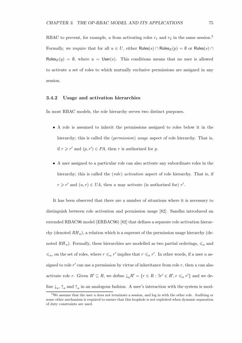
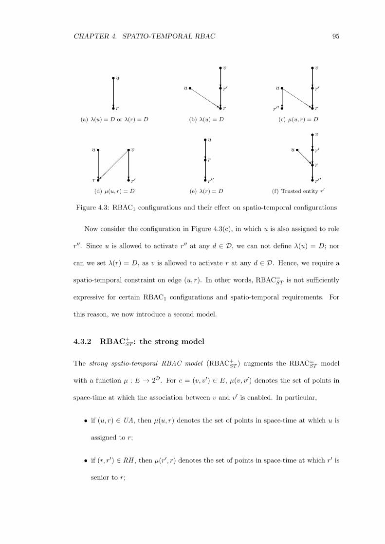
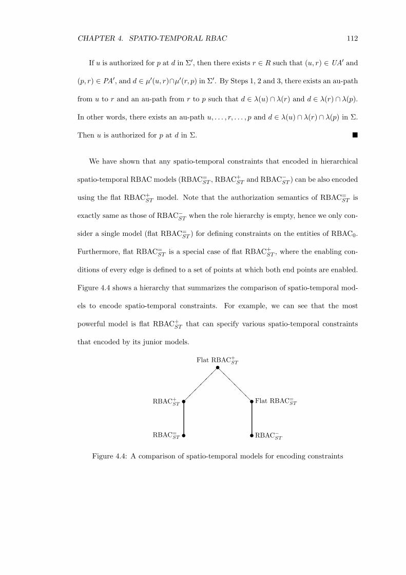
spatio-temporal constraints [76] on various components of the standard RBAC model.

However, the syntax for these models is rather complicated and the semantics defining

the interaction between spatio-temporal constraints and the role hierarchy are not

clearly defined. In other words, no existing work has clear authorization semantics

in terms of how access requests will be answered in the presence of a role hierarchy

and spatio-temporal constraints. Moreover, no existing work assesses the difficulties of

implementing these models in practical applications.

We believe that it is important to consider the effect of spatio-temporal constraints

on RBAC. In particular, we believe that any spatio-temporal RBAC model should have

clear and unambiguous semantics. Hence, it is important to examine the question of

how can we develop new spatio-temporal RBAC models with simple syntax and ap-

propriate semantics which explicitly consider the relationship between spatio-temporal

constraints and role hierarchies. Having developed spatio-temporal RBAC models, it

is also crucial to consider the implementation of these models in practical settings.

1.1.4 Computational problems in RBAC

Just as the development of new RBAC models has led to interesting questions about

authorization semantics, new applications and models for RBAC have given rise to a

number of interesting computational problems. Joshi et al recently raised an important

problem – the inter-domain role mapping (IDRM) problem [36] – when GTRBAC is

employed in distributed environments. Their statement of the IDRM problem is to find

a set of roles of minimal cardinality such that the authorized permissions for that set of

roles is precisely the set of requested permissions. This problem was further extended


to the user authorization query (UAQ) problem [94, 96].

On the other hand, Li et al recently studied a number of interesting problems

with regard to separation of duty constraints and their enforcement in the context of

RBAC [65]. One of the problems – the role-based static separation of duty constraint

(RSSoD) generation problem – is of particular importance when translating restrictions

on permissions expressed in separation of duty constraints to restrictions on role mem-

berships in RBAC. The RSSoD generation problem asks given a set of permissions,

find all possible sets of roles such that each set of roles is collectively authorized for the

given set of permissions, and any proper subset of that set of roles is not.

However, existing work does not always pose the most appropriate problem, as is

the case with the IDRM problem of Du and Joshi [36]. It is easy to show that the

IDRM problem is not well-defined, in the sense that many instances of the problem

may not have a solution. Moreover, none of the above problems has been properly

analyzed and solved. In particular, the IDRM problem and the UAQ problem were

conjectured to be NP-hard without establishing a formal proof, and directly suggested

heuristic algorithms to produce a solution [36, 94, 96]. Nevertheless, if these problems

have not been proved to be NP-hard, there is no way of ensuring there do not exist

efficient algorithms to solve them. In addition, the computational complexity of the

RSSoD generation problem has not been established. In summary, we are unaware of

any attempt to formally assess the computational complexity of the above problems,

which we believe is an important step in understanding and solving the problems.

1.2 Contributions

There is a substantial body of work on RBAC, much of it involving role hierarchies. As

we described in the previous section, the consequences of including those hierarchies are


rarely properly explored. In this thesis, we investigate a number of related problems:

the perceived limitations of the inheritance semantics of a role hierarchy, the relation-

ship between permission usage and role activation hierarchies, the interaction between

spatio-temporal constraints and inheritance, and the computational complexity of sev-

eral problems arising in hierarchical RBAC. Unlike existing work in these areas, we

strive for compatibility with RBAC96 and precise authorization semantics. We now

describe the contributions of the thesis, and briefly explain their significance compared

with the existing work.

The oriented permission RBAC model (OP-RBAC) developed by Crampton [29]

proposed a new mechanism for permission inheritance within a role hierarchy, and was

considered to provide more flexibility than standard role-based models. We explore how

OP-RBAC can address the perceived shortcomings of the standard RBAC approach

to inheritance. In particular, we illustrate that OP-RBAC provides a natural way

to simulate a number of Bell-LaPadula models, and to enforce dynamic separation of

duty constraints. The simplicity of our approach compares favourably with previous

attempts, which typically require multiple role hierarchies and support only limited

features of the Bell-LaPadula model.

We then turn our attention to supporting multiple hierarchies in RBAC. We propose

a novel extended RBAC model, called ERBAC07, which defines an alternative way to

distinguish permission usage and role activation hierarchies. Unlike ERBAC96 and

GTRBAC, our approach to defining these hierarchies is based on their inheritance

semantics. The syntax we have chosen for ERBAC07 is consistent with RBAC96, and

the semantics for the model is extended from our graph-based formalism of RBAC96.

In other words, ERBAC07 is compatible with RBAC96 and has a clear authorization

semantics.

Having established an extended RBAC model supporting permission usage and role


activation hierarchies, it is natural to then address the question of constraints that may

interact with those hierarchies. In particular, we extend the RBAC96 and ERBAC07

models by defining two spatio-temporal constraint specification functions. We use these

two functions to define three spatio-temporal RBAC models with different authorization

semantics. Compared with existing work, such as GTRBAC and the spatio-temporal

model of Ray and Toahchoodee – the only models dealing with multiple role hierarchies

and spatio-temporal constraints – our models are concise and have precise authorization

semantics. We also propose strategies for the use of our spatio-temporal RBAC models

in practical applications, which no existing work has attempted to do.

Finally, we introduce a mathematical framework where we define a number of com-

putational problems that are variations on the standard set cover problem. In partic-

ular, we define the minimal cover problem, and prove that this problem is NP-hard.

This result enables us to establish computational complexity for some important prob-

lems in the context of RBAC. We also design a number of heuristic algorithms for the

minimal cover problem and conduct experiments to evaluate the quality of these algo-

rithms. Our experiment results enable us to identify a good heuristic algorithm with

high success rates to compute an exact solution to the minimal cover problem.

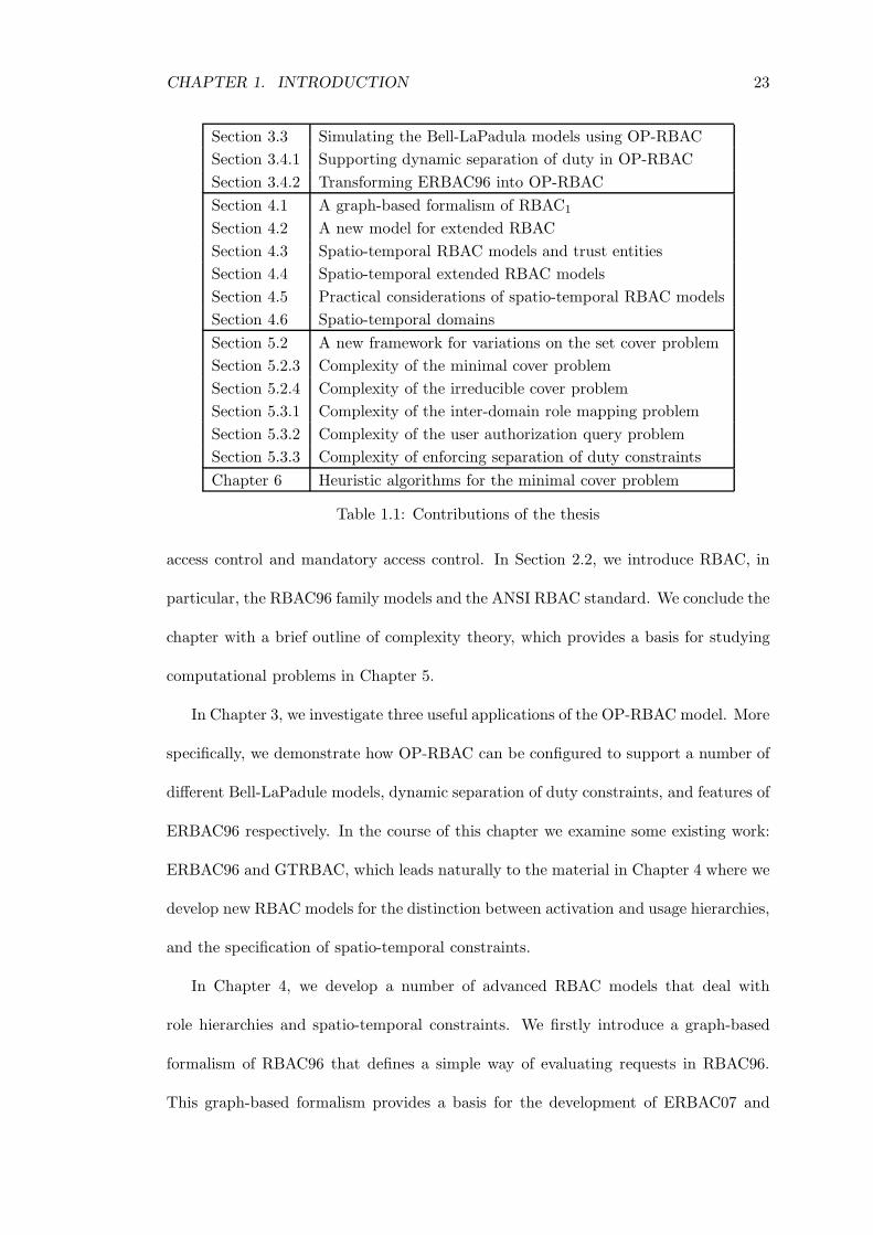
We summarize the contributions of this thesis in Table 1.1 that indicates the section

in which each contribution appears.

1.3 Structure of the thesis

The remainder of the thesis is organized as follows.

In Chapter 2, we introduce some prerequisite concepts in access control, RBAC and

complexity theory. In Section 2.1, we make explicit distinctions between access control

policies, states, models and mechanisms, and clarify these distinctions in discretionary


Section 3.3 Simulating the Bell-LaPadula models using OP-RBAC

Section 3.4.1 Supporting dynamic separation of duty in OP-RBAC

Section 3.4.2 Transforming ERBAC96 into OP-RBAC

Section 4.1 A graph-based formalism of RBAC1

Section 4.2 A new model for extended RBAC

Section 4.3 Spatio-temporal RBAC models and trust entities

Section 4.4 Spatio-temporal extended RBAC models

Section 4.5 Practical considerations of spatio-temporal RBAC models

Section 4.6 Spatio-temporal domains

Section 5.2 A new framework for variations on the set cover problem

Section 5.2.3 Complexity of the minimal cover problem

Section 5.2.4 Complexity of the irreducible cover problem

Section 5.3.1 Complexity of the inter-domain role mapping problem

Section 5.3.2 Complexity of the user authorization query problem

Section 5.3.3 Complexity of enforcing separation of duty constraints

Chapter 6 Heuristic algorithms for the minimal cover problem

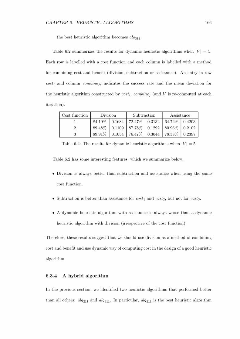
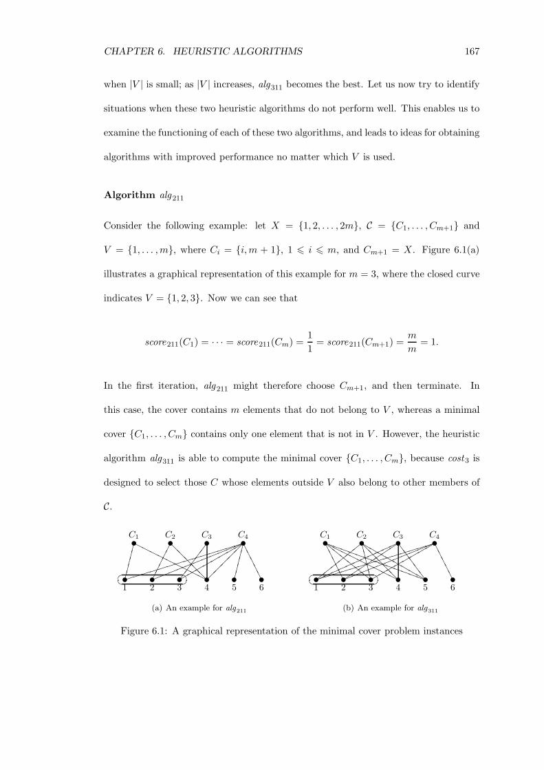
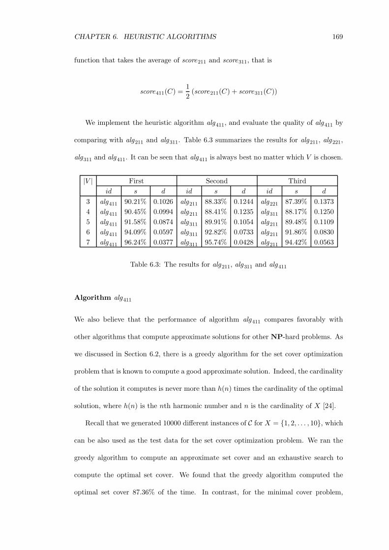
Table 1.1: Contributions of the thesis

access control and mandatory access control. In Section 2.2, we introduce RBAC, in

particular, the RBAC96 family models and the ANSI RBAC standard. We conclude the

chapter with a brief outline of complexity theory, which provides a basis for studying

computational problems in Chapter 5.

In Chapter 3, we investigate three useful applications of the OP-RBAC model. More

specifically, we demonstrate how OP-RBAC can be configured to support a number of

different Bell-LaPadule models, dynamic separation of duty constraints, and features of

ERBAC96 respectively. In the course of this chapter we examine some existing work:

ERBAC96 and GTRBAC, which leads naturally to the material in Chapter 4 where we

develop new RBAC models for the distinction between activation and usage hierarchies,

and the specification of spatio-temporal constraints.

In Chapter 4, we develop a number of advanced RBAC models that deal with

role hierarchies and spatio-temporal constraints. We firstly introduce a graph-based

formalism of RBAC96 that defines a simple way of evaluating requests in RBAC96.

This graph-based formalism provides a basis for the development of ERBAC07 and


spatio-temporal RBAC models in this chapter. We also suggest some approaches to

facilitate the implementation of our spatio-temporal RBAC models.

Joshi et al [36] introduced the inter-domain role mapping problem in the context

of multiple role hierarchies and temporal constraints. The analysis of this problem

motivates us to study some computational problems in Chapter 5. We firstly define

some variations on the standard set cover problem, and establish their computational

complexity. Then we apply these complexity results to some important problems in

RBAC, including the inter-domain role mapping problem, the user-authorization query

problem and the separation of duty constraints enforcement problem.

As the minimal cover problem defined in Chapter 5 has been proved to be NP-

hard, Chapter 6 is concerned with the design and evaluation of heuristic algorithms for

solving the problem.

Finally, in Chapter 7, we review the contributions of the thesis and discuss oppor-

tunities for future work.

1.4 Publications

A list of publications describing some of the research results contained in this thesis is

provided below.

• L. Chen and J. Crampton. Applications of the oriented permission role-based

access control model. In proceedings of the 26th IEEE International Performance

Computing and Communications Conference, pages 387-394, 2007.

• L. Chen and J. Crampton. Inter-domain role mapping and least privilege. In Pro-

ceedings of the 12th ACM Symposium on Access Control Models and Technologies,

pages 157-162, 2007.


• L. Chen and J. Crampton. On spatio-temporal constraints and inheritance in role-

based access control. In Proceedings of the 2008 ACM Symposium on Information,

Computer and Communications Security, pages 205-216, 2008.

• L. Chen and J. Crampton. Set covering problems in role-based access control. In

Proceeding of the 14th European Symposium on Research in Computer Security,

pages 689-704, 2009.

Chapter 2

Background

The main purpose of this chapter is to introduce relevant background material. In

Section 2.1 we give a brief introduction to some basic concepts and earlier developments

in access control. In particular, we introduce the two best known types of access

control – discretionary access control and mandatory access control – which serve as

a motivation for role-based access control and inform the material in Chapter 3. In

Section 2.2 we introduce role-based access control and review the RBAC96 family of

models and the ANSI RBAC standard, which is fundamental to the remainder of this

thesis. We conclude the chapter with a brief outline of complexity theory that will

be required in Chapters 5 and 6 when we study some computational problems in the

context of role-based access control.

2.1 Access control

One of the essential security services in (multi-user) computer systems is access con-

trol, a mechanism for constraining the interaction between (authenticated) users and

protected resources. In the context of computer systems, access control may also be

referred to as authorization. Generally, access control is concerned with controlling

26

CHAPTER 2. BACKGROUND 27

which users have access to which resources in computer systems. Given a computer

system, access control can be implemented in many places and at different levels [3, 39].

Operating systems implement access control to limit access to files, directories and de-

vices. Database management systems apply access control to regulate access to tables

and views. Sensitive applications incorporate access control to ensure some application

functions are only available to certain users and other applications. Moreover, access

control can take many forms, which means in addition to checking whether a user is

authorized to access a resource, access control may also be concerned with constrain-

ing when, where and how a resource can be used. For example, in the context of the

financial sector, (i) financial managers might have access to some sensitive reports only

during working hours and at certain offices, and (ii) to prevent fraud, we may require

that a financial manager is not allowed to approve a loan that was created by herself.

When implementing access control in computer systems, it is important to un-

derstand and distinguish four concepts: access control policies, access control states,

access control models and access control mechanisms [32, 34, 78]. Access control is

often “policy-based” in the sense that a user’s request to access a resource (an access

request) is checked to see if it is authorized by a policy. Access control policies gen-

erally specify who is authorized to access which resources under what circumstances.

In other words, access control policies define rules for deciding whether access requests

should be granted or not. The conditions that determine whether an access request is

authorized are usually defined in terms of the (access control) state or configuration

of the computer system. The state of the system is a snapshot of all security-relevant

information at a point in time; the state may change over time. Consider, for example,

the simple security property defined in the Bell-LaPadula access control model [12],

which says that a user u is authorized to read a document d only if λ(u) > λ(d), where

λ : U ∪D → L is a labeling function and (L,6) is a lattice of security labels. Infor-


mally, the policy states that a user is authorized to read a document only if the user’s

security level is at least as high as that of the requested document. The state is defined

by the security lattice L and the security function λ. Crampton recently defined the

distinction between access control policy and state as shown in the following quote [32].

“An access control policy is a specification of decision-marking function that

takes a request query and access control state as inputs and returns an access

control decision.”

By definition, the evaluation of an access control policy is dependent on the access

request and the current access control state of the system. An obvious example is

the Chinese Wall policy [18], which is designed to prevent a user from accessing docu-

ments whose owners belonging to a conflict interest class. The evaluation of this policy

depends on the mutable system state: namely, historical information about which doc-

uments the user have previously accessed.

In summary, it is important to make a clear distinction between policy and state, be-

cause such distinction provides reuse of already existing authorization decision functions

(policies) and separates the specification of access control state from policy semantics.

We use the term authorization syntax for the language that is used to specify states,

and authorization semantics for the effect of evaluating a policy for a given request and

state. Equivalently, we could regard the semantics of a state (with respect to a fixed

policy) to be the set of requests that are authorized by the state.

An access control model is an abstract mathematical description of authorization

syntax, together with a definition of authorization semantics. More specifically, it

defines a collection of sets, functions and relations that provide a method for encoding

access control states, and specifies the conditions that must be satisfied for an access

request to be granted [31]. The RBAC96 model is a typical example of an access


control model, which we will introduce in Section 2.2. Informally, an access control

model provides a blueprint for the implementation of access control systems. It may

also provide assurances of security for an implemented system, an example being the

famous security theorem of the Bell-LaPadula model [12].

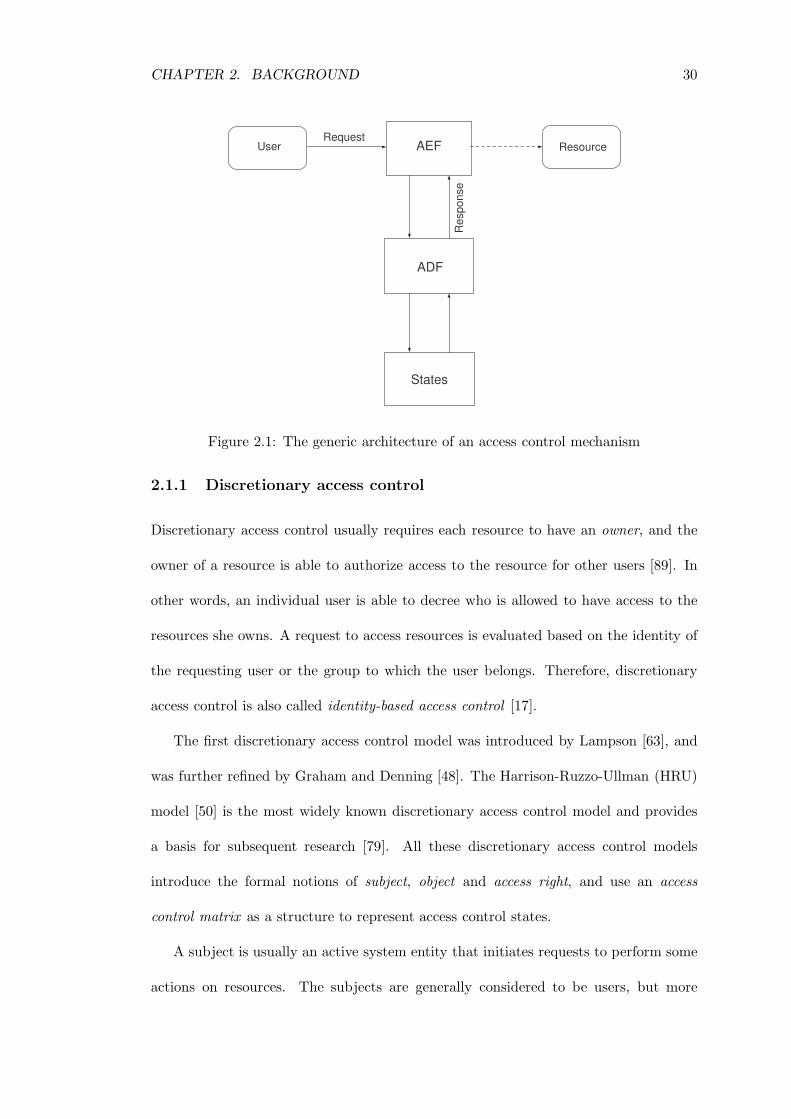
An access control mechanism (also known as a reference monitor or an authoriza-

tion service) is a computer function that implements the controls formally stated in

the access control model. However, it is often difficult to provide an access control

mechanism that correctly and completely implements the access control model. In gen-

eral, any access control mechanism includes two distinct components: the authorization

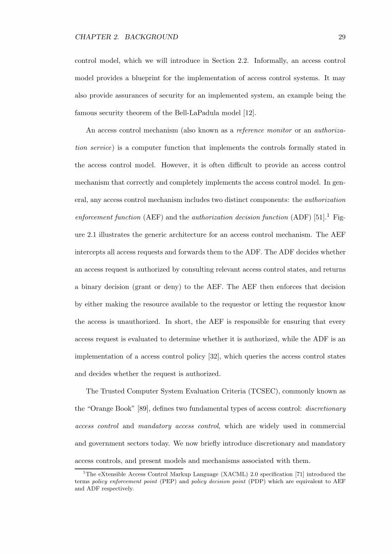
enforcement function (AEF) and the authorization decision function (ADF) [51].1 Fig-

ure 2.1 illustrates the generic architecture for an access control mechanism. The AEF

intercepts all access requests and forwards them to the ADF. The ADF decides whether

an access request is authorized by consulting relevant access control states, and returns

a binary decision (grant or deny) to the AEF. The AEF then enforces that decision

by either making the resource available to the requestor or letting the requestor know

the access is unauthorized. In short, the AEF is responsible for ensuring that every

access request is evaluated to determine whether it is authorized, while the ADF is an

implementation of a access control policy [32], which queries the access control states

and decides whether the request is authorized.

The Trusted Computer System Evaluation Criteria (TCSEC), commonly known as

the “Orange Book” [89], defines two fundamental types of access control: discretionary

access control and mandatory access control, which are widely used in commercial

and government sectors today. We now briefly introduce discretionary and mandatory

access controls, and present models and mechanisms associated with them.

1The eXtensible Access Control Markup Language (XACML) 2.0 specification [71] introduced theterms policy enforcement point (PEP) and policy decision point (PDP) which are equivalent to AEFand ADF respectively.


Resource

Re

sp

on

se

AEFUserRequest

ADF

States

Figure 2.1: The generic architecture of an access control mechanism

2.1.1 Discretionary access control

Discretionary access control usually requires each resource to have an owner, and the

owner of a resource is able to authorize access to the resource for other users [89]. In

other words, an individual user is able to decree who is allowed to have access to the

resources she owns. A request to access resources is evaluated based on the identity of

the requesting user or the group to which the user belongs. Therefore, discretionary

access control is also called identity-based access control [17].

The first discretionary access control model was introduced by Lampson [63], and

was further refined by Graham and Denning [48]. The Harrison-Ruzzo-Ullman (HRU)

model [50] is the most widely known discretionary access control model and provides

a basis for subsequent research [79]. All these discretionary access control models

introduce the formal notions of subject, object and access right, and use an access

control matrix as a structure to represent access control states.

A subject is usually an active system entity that initiates requests to perform some

actions on resources. The subjects are generally considered to be users, but more


precisely, they are processes or threads that execute under the control of a computer

system. An object is usually a passive system entity that can be any resource to which

access should be retrieved. Typical examples of objects in operating systems include

files, directories and printers. An access right is an action that is invoked by subjects

on objects. Typical examples of access rights in an operating system include read, write

and execute.

An access control matrix M (also known as a protection matrix ) has rows indexed

by subjects and columns indexed by objects. The matrix entry for subject s and object

o, denoted Ms,o, contains a set of access rights for which s is authorized with respect

to o. An access request is modeled as a triple (s, o, a), and is authorized if, and only if,

a ∈Ms,o. Table 2.1 represents a simple access control matrix, where the file diary.doc

can be read and written by Bob while Alice has no access at all. In addition, Bob is an

owner of diary.doc and he can allow Alice to read diary.doc by entering the right

read into the entry [Alice, diary.doc] in the matrix.

bill.doc diary.doc install.exe

Bob {read} {own, read, write} {execute}

Alice {read, write} – {execute}

Table 2.1: An access control matrix

An access control matrix will become very large and the non-empty entries will be

sparse in a computer system with large numbers of users and resources. In this case,

it might not only cause performance problems but also be vulnerable to administrative

errors. Therefore, an access control matrix is rarely implemented in a computer system.

Instead, two popular discretionary access control mechanisms store the access control

matrix either by columns (access control lists) or rows (capability lists).

An access control list is associated with an object, and consists of zero or more access

control entries. Each access control entry specifies a subject and the set of access rights


for which that subject is authorized. In contrast, a capability list is associated with a

subject, and contains a list of permissions. Each permission identifies an object and a

set of access rights that have been assigned to the subject for that object. In Figure 2.1,

for example, principal Bob has the capability to read object bill.doc. In other words,

an access control list is concerned with what may be done with an object. In modern

operating systems, access control lists are commonly used to protect files and resources.

On the other hand, a capability list is concerned with what a subject is allowed to do.

It is usually incorporated in application-oriented IT systems that focus on controlling

the actions of subjects.

2.1.2 Mandatory access control

Mandatory access control is deployed when the use of resources is determined by the

characteristics of the resource and the subject, not the wishes of the owner. The

characteristics of the subject and the object are often represented by security levels

assigned to subjects and objects in the system. The security level of a subject, also

called the clearance level of the subject, reflects the level of trust assigned to the subject,

while the security level of an object, also called the classification level of the object,

reflects the level of sensitivity of the contents of the object. The set of security levels is

partially ordered and is often assumed to form a lattice [80]. Thus, a computer system

that implements mandatory access control is often called a multi-level secure system.

The act of accessing an object can be regarded as initiating an information flow. In

particular, read access can be seen as a flow of information from object to subject, while

write access is a flow of information from subject to object. An mandatory information

flow policy for confidentiality requires that high level information cannot flow to a lower

level.2 In other words, the information flow policy requires that a subject is only allowed

2To safeguard the integrity of information, Biba proposed a dual policy that low level integrity


to read an object if the subject’s security level is at least as high as that of the object,

and a subject is only allowed to write an object if the object’s security level is at least

as high as that of the subject. These two requirements are usually called “no-read-up”

policy and “no-write-down” policy, respectively. In practice, in order to define all the

authorization requirements of a computer system, mandatory information flow policy

is usually augmented with a discretionary access control policy that is defined by the

object owners and implemented using a protection matrix [12].

The Bell-LaPadula model has been the subject of extensive research in several

seminal papers [8, 10, 11, 12] and is perhaps the best known of all access control models.

It provides a combination of mandatory access control and discretionary access control.

We formally introduce a simplified version of the Bell-LaPadula model [10, 11] by

defining a set of subjects S, a set of objects O, an access control matrixM with columns

indexed by O and rows indexed by S, a partially ordered set of security labels (L,6), a

security function λ : S∪O→ L3, and a set of access rights A = {read, append, write},

where read denotes read only access, append denotes write only access and write

denotes both read and write access. The state of a Bell-LaPadula system is defined

to be (V,M), where V represents the set of active triples of the form (s, o, a), where

s ∈ S, o ∈ O, and a ∈ {read, append, write}; that is, the set of access requests that

have been granted by the access control mechanism [10].

To enforce a mandatory information flow policy and a discretionary access control

policy, every state of a Bell-Lapadula system must satisfy three security properties: the

simple security property, the *-property and the discretionary security property.

• A state (V,M) satisfies the simple security property if for all (s, o, read) ∈ V ,

information is not allowed to flow to a higher level [16]. In this chapter, we only consider informationflow policies in the Bell-LaPadula model, because the formulation of the Biba integrity model is thedual of that in the Bell-LaPadula model.

3We assume that the labelling of entities is performed by a single security function λ, and thesecurity function λ is fixed


λ(s) > λ(o). In other words, the simple security property is satisfied if every

granted read access (that is, belongs to V ) was authorized by the “no-read-up”

policy.

• A state (V,M) satisfies the *-property if for all (s, o, append) ∈ V , λ(s) 6 λ(o).

In other words, the *-property is satisfied if every granted append access was

authorized by the “no-write-down” policy.4

• A state (V,M) satisfies the discretionary security property if for all (s, o, a) ∈

V , a ∈ Ms,o. In other words, every access request that has been granted was

authorized by an appropriate entry in the access control matrix.

In actual fact, the Bell-LaPadula model [12] makes use of three security functions to

label subjects and objects, and the simple security property and the *-property are

defined in terms of those three security functions. We will introduce a more complete

version of the Bell-LaPadula model in Chapter 3 when studying the simulation of the

Bell-LaPadula models using role-based methods.

The Bell-LaPadula model has been implemented in military applications and com-

mercially sensitive applications [17]. Multics is considered to be the best example of an

operating system built for security [17], in which the protection mechanisms basically

implement the Bell-LaPadula model.

2.2 Role-based access control

Role-based access control has received considerable attention in recent years, and is

widely accepted as an alternative to discretionary and mandatory access controls [39].

4The *-property in the original formulation of the Bell-LaPadula model [10] requires that for all(s, o, read) ∈ V , and for all (s, o′, append) ∈ V , λ(o) 6 λ(o′). The *-property we introduce here is themost commonly accepted version (see [73, 80]), and is slightly stronger than the *-property definedin the original Bell-LaPadula model [10]. In Chapter 3, we consider more complex version of the*-property.


The motivation for the development of role-based access control is to address the per-

ceived deficiencies of existing discretionary and mandatory access control models in

terms of specification and enforcement of organization-specific access control policies,

and to reduce the complexity and cost of administering systems based on these mod-

els [44]. In other words, neither discretionary nor mandatory access control is suffi-

ciently suitable for the needs of most commercial systems. More specifically, discre-

tionary access control, for example, permits users to grant or revoke access to any of

the objects they owned. However, for many organizations within industry and civilian

government, the corporation or agency is the owner of system objects, rather than the

end users [44]. Hence, it is not appropriate to allow users to pass access rights on the

objects to other users in these organizations. Mandatory access control that focuses

on preserving confidentiality is too restrictive and therefore inappropriate for these or-

ganizations as well. In addition, in an organization with a large and dynamic user

population, it is time-consuming and error-prone to manage an access control system

based on access control lists. In particular, it is extremely difficult to revoke a user’s

access permissions, because it involves checking the access control lists of all objects in

the system.

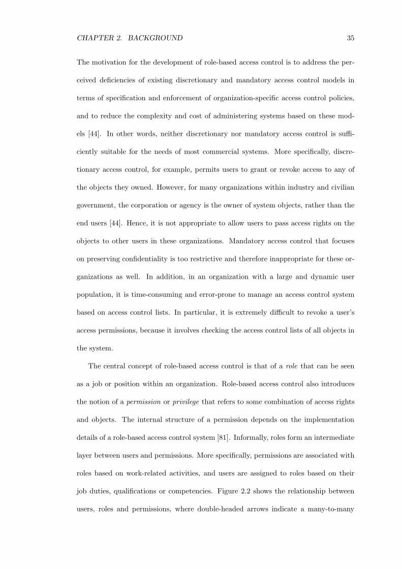
The central concept of role-based access control is that of a role that can be seen

as a job or position within an organization. Role-based access control also introduces

the notion of a permission or privilege that refers to some combination of access rights

and objects. The internal structure of a permission depends on the implementation

details of a role-based access control system [81]. Informally, roles form an intermediate

layer between users and permissions. More specifically, permissions are associated with

roles based on work-related activities, and users are assigned to roles based on their

job duties, qualifications or competencies. Figure 2.2 shows the relationship between

users, roles and permissions, where double-headed arrows indicate a many-to-many


relationship. For example, a user can be assigned to one or more roles, and a role can

have one or more user members. This arrangement of controlling access through roles

provides great flexibility and simplifies the management of access controls. For example,

within a large organization, as job assignments and organizational functions change,

we can simply adjust user-role association and permission-role association respectively,

rather than allocating permissions to each user on an individual basis.

Users Roles Access rightsObjects

Permissions

Figure 2.2: A simple relationship between users, roles and permissions

Role-based access control has been the subject of considerable research in the last

decade, resulting in the development of a number of different role-based access control

models. Ferraiolo and Kuhn developed the first formal role-based access control model

in 1992 [40], and then introduced further refinement in 1995 [38]. Nyanchama and

Osborn proposed a role graph model [70] that organizes roles using a graph, and the

role graph model has led to subsequent research over the years [92, 93]. The RBAC96

family of models [83], due to Sandhu et al , is undoubtedly the most well known model

for RBAC, and provides the basis for the recent ANSI RBAC standard [2]. In this

thesis, we will focus on the RBAC96 model and the ANSI RBAC standard.

2.2.1 RBAC96

The RBAC96 family of models consists of four conceptual models that form a hierarchy

as shown in Figure 2.3. The simplest model, RBAC0, introduces the basic features of

role-based access control. RBAC1 and RBAC2 extend RBAC0 through the addition of

role hierarchy and constraints respectively. RBAC3 includes all the features of RBAC1


and RBAC2.

tRBAC0

tRBAC1tRBAC2

tRBAC3

ZZZZZZZZ

��

��

ZZZZZZZZ

Figure 2.3: The RBAC96 family of models

RBAC0

RBAC0 defines a set of users U , a set of roles R, a set of permissions P , a user-role

assignment relation UA ⊆ U×R and a permission-role assignment relation PA ⊆ P×R.

We refer to such sets and relations as components of RBAC0. We write Roles(u) for

the set of roles to which a user u is explicitly assigned by the UA relation; that is,

Roles(u) = {r ∈ R : (u, r) ∈ UA}. Similarly, we write Roles(p) for the set of roles to

which a permission p is explicitly assigned by the PA relation; that is, Roles(p) = {r ∈

R : (p, r) ∈ PA}. Given r ∈ R, we write Prms(r) to denote the set of permissions for

which r is explicitly assigned, and for R′ ⊆ R, we write Prms(R′) to denote the set of

permissions for which the roles in R′ are explicitly assigned. That is,

Prms(r) = {p ∈ P : (p, r) ∈ PA} and Prms(R′) =⋃

r∈R′

Prms(r).

RBAC0 also introduces the concept of a session that is synonymous with a subject in

traditional access control models. When a user logs in to a computer system (employing

a role-based access control mechanism), the user can establish a session during which

she can activate a subset of roles to which she is explicitly assigned. A user may run

multiple sessions simultaneously, and each session may have a different combination


of active roles. We denote the set of sessions by S, and the user who established the

session s ∈ S by User(s). We write Roles(s) for the set of roles activated in a session s,

that is, Roles(s) ⊆ Roles(u), where u = User(s). A request by u to invoke permission p

in session s is granted if u has activated one of p’s explicitly assigned roles in s, that

is, Roles(s) ∩ Roles(p) 6= ∅.

RBAC1

RBAC1 introduces the concept of a role hierarchy, which is modeled as a partial order

on the set of roles. In other words, the role hierarchy is a binary relation RH ⊆ R×R

that is reflexive, anti-symmetric and transitive. We write r 6 r′ if (r, r′) ∈ RH and

r < r′ if r 6 r′ and r 6= r′. The role hierarchy is used to reduce the administrative

burden by reducing the number of explicit assignments in the UA and PA relations.

That is, if (u, r) ∈ UA and r′ 6 r, then u is implicitly assigned to r′; and if (p, r) ∈ PA

and r 6 r′ then p is implicitly assigned to r′.

Given r ∈ R, we write ↓r to denote the set of all elements in R that are less than or

equal to r: that is, ↓r = {r′ ∈ R : r′ 6 r}. Similarly, we write ↑r = {r′ ∈ R : r 6 r′}.

We write ↓Roles(u) to denote the set of roles explicitly and implicitly assigned to u,

that is

↓Roles(u) = {r′ ∈ R : ∃r ∈ Roles(u), r′ 6 r}.

Similarly, we write ↑Roles(p) to denote a set of roles explicitly and implicitly assigned

to p, that is

↑Roles(p) = {r′ ∈ R : ∃r ∈ Roles(p), r 6 r′}.

Note that henceforth we will write “authorized” to mean “explicitly and implicitly

assigned”. We write Prms(↓r) for the set of permissions for which r is authorized.

We now analyze the use of sessions in RBAC1. A user u is allowed to establish


a session s to activate a set of roles that can be any subset of roles for which she is

authorized, that is, Roles(s) ⊆ ↓Roles(u), where u = User(s). A request by u to invoke

permission p in session s is granted if u has activated one of p’s authorized roles in s, that

is Roles(s) ∩ ↑Roles(p) 6= ∅. Providing that RH = {}, we have Roles(s) ⊆ ↓Roles(u) =

Roles(u) and ↑Roles(p) = Roles(p). In this case, we recover RBAC0 authorization

semantics. In other words, RBAC0 is a special case of RBAC1 in which the hierarchy

relation is empty.

RBAC2

RBAC2 extends RBAC0 by introducing constraints, which usually specifies a set of

forbidden configurations of an access control system. RBAC2 informally discussed three

types of constraints that can be defined over the components of RBAC0: dependency

constraints, cardinality constraints and separation of duty constraints. Dependency

constraints may specify that certain roles can be activated only if the requesting user has

already activated some other roles. Cardinality constraints may specify the maximum

number of users that can be assigned to or activate a role, and the maximum number

of roles that can be activated in a session by a user. Dependency and cardinality

constraints in role-based access control have received little attention in the literature,

and support for these constraints was dropped in the ANSI RBAC standard.

Separation of duty is a widely recognized business principle that is used to prevent

conflict of interests arising or to prevent fraudulent actions. It requires that more than

one user be involved in the execution of two or more tasks in a business process, which,

if performed by the same user, could expose the process to misuse. Early work on

separation of duty constraints in computer systems includes the Chinese Wall security

policy, which prohibits any user from having access to documents belonging to two

different competitors [18]. In RBAC2, separation of duty constraints are supported by


defining mutually exclusive roles. Generally, the set of permissions that are required

to perform sensitive tasks are assigned to mutually exclusive roles, and no user can be

assigned to more than one role in the mutually exclusive set, or no user is allowed to

activate more than one role in the set. Simon and Zurko [84] refer to the former as

static separation of duty, and to the latter as dynamic separation of duty. The research

community has since taken an active interesting in proposing specification schemes for

separation of duty constraints in role-based access control [1, 15, 30, 45, 52, 70, 84],

and suggesting models for enforcing such constraints [15, 30, 65, 70, 84].

RBAC3

RBAC3 incorporates the features of RBAC1 and RBAC2. It is known that there exists

a certain “tension” between separation of duty constraints and a role hierarchy. In the

simplest case, if p and q are mutually exclusive permissions, then p and q should be

assigned to two different incomparable roles r and r′. The separation of duty between

two roles r and r′ is impossible to realize if r and r′ have a common senior role r′′,

because r′′ inherits the permissions of both roles. If we require that no user is allowed

to be assigned to or activate r′′, then there is no point in having the “unassignable”

role r′′ in the role hierarchy. A number of extended role-based access control models,

which we discuss in Chapter 3 and 4, have been introduced to address this shortcoming

of RBAC3.

2.2.2 ANSI-RBAC

The American National Standard Institute (ANSI) standard for role-based access con-

trol (RBAC) [2] provides a consistent and uniform definition of RBAC features, and

gives information technology vendors a guideline for designing RBAC products. The

ANSI RBAC standard includes three components: Core RBAC, Hierarchical RBAC,


and Constrained RBAC.

Core RBAC defines the basic building blocks of a RBAC system: a set of basic

element sets U , S, R and P , a set of relations UA and PA, and a set of mapping

functions shown in the top part of Table 2.2. The table uses ANSI RBAC syntax

rather then the RBAC96-style syntax we used in the previous section, but we can

easily extend our notation to define these functions if desired.

Core Component

assigned users(r) = {u ∈ U : (u, r) ∈ UA}

assigned permissions(r) = {p ∈ P : (p, r) ∈ PA}

session users(s) = u

session roles(s) ⊆ {r ∈ R : (session users(s), r) ∈ UA}

avail session perms(s) =⋃

r∈session roles(s) assigned permissions(r)

Hierarchical RBAC

authorized users(r) = {u ∈ U : r 6 r′, (u, r′) ∈ UA}

authorized permissions(r) = {p ∈ P : r > r′, (p, r′) ∈ PA}

Proposed extensions for Hierarchical RBAC

session roles(s) ⊆ {r ∈ R : r 6 r′, (session users(s), r′) ∈ UA}


r∈session roles(s) authorized permissions(r)

Table 2.2: ANSI-RBAC mapping functions

Hierarchical RBAC introduces role hierarchies that are intended to reflect the hier-

archical nature of many organizations and thereby simplify access control management.

There are two types of role hierarchies defined in the hierarchical component: general

role hierarchies and limited role hierarchies. The general role hierarchy is an arbitrary

partial order on the set of roles R. The limited role hierarchy is defined to be an

inverted tree structure, where each role has only a single immediate child. It is inter-

esting to note that separation of duty constraints are compatible with the limited role

hierarchy: the separation of duty constraint between two incomparable roles r and r′

can be enforced, because there does not exist a common senior role r′′ of r and r′ in

the limited role hierarchy.


In addition, the hierarchical component defines two functions authorized users

and authorized permissions, shown in the second section of Table 2.2. The standard

states that r 6 r′ only if authorized permissions(r) ⊆ authorized permissions(r′)

and authorized users(r′) ⊆ authorized users(r). The core component defines func-

tions avail session perms and session roles, shown in the first section of Table 2.2,

but no analogous function is defined for the hierarchical component, which is a cu-

rious omission. We propose new definitions for the functions session roles and

avail session perms for the hierarchical component. These definitions are shown in

the third section of Table 2.2. Note that in core RBAC, assigned permissions(r) =

authorized permissions(r) for all r. Hence, our definition is consistent with that given

in the core component.

Constrained RBAC introduces two types of separation of duty constraints: Static

Separation of Duty (SSD) and Dynamic Separation of Duty (DSD). A SSD constraint

is specified as a pair (R′, n), where R′ ⊆ R and 2 6 n 6 |R′|, and can be defined in

Core RBAC and Hierarchical RBAC. The SSD constraint (R′, n) is satisfied by Core

RBAC if no user is assigned to n or more roles in the set R′, while the SSD constraints

(R′, n) is satisfied by hierarchical RBAC if no user is authorized for n or more roles

in the set R′. Like SSD, a DSD constraint is written as (R′, n), where R′ ⊆ R and

2 6 n 6 |R′|, which limits the roles that a user can activate in one session. Specifically,

the DSD constraint is satisfied if no user may simultaneously activate n or more roles

from R′ in one session. Clearly, satisfaction of a SSD constraint is simply enforced by

checking the number of roles in R′ for which each user is authorized. Similarly, it is

simple to check whether a DSD constraint is satisfied by computing the number of roles

in R′ that is activated in each session.

Li et al recently identified a number of design flaws and technical errors for the ANSI

RBAC standard and suggested some improvements to the standard [64]: the standard


should remove the notion of sessions from the core component, and specify only one

role can be activated in a session; the standard should introduce a new approach for

modelling the role hierarchy so as to facilitate the changes to the role hierarchy; and

the standard should clearly specify and discuss the semantics of role hierarchy in terms

of user inheritance, permission inheritance and activation inheritance. The authors of

the original proposal for the ANSI-RBAC standard responded to each suggestion and

clarified the rationale for the choices they made in the standard [41].

2.3 Complexity theory

In this section, we give a brief introduction to compleixity theory, which provides a basis

for studying some fundamental problems in role-based access control in Chapter 5 and

Chapter 6.

The study of computational problems is one of the main subjects in theoretical

computer science. In general, a (computational) problem φ can be expressed in terms

of some relation φ ⊆ Iφ × Sφ, where Iφ is the set of problem instances and Sφ is the

set of problem solutions. A (deterministic) algorithm is said to solve a problem φ if

that algorithm is guaranteed always to produce a solution for any instance i of φ.

Given a problem φ, clearly, we are interested in finding the most efficient algorithm for

solving the problem. The efficiency of an algorithm can be measured by the time and

memory required to execute the algorithm. In this thesis, we only concentrate on time

requirements when measuring the efficiency of algorithms.

The worst-case time complexity for an algorithm is a function ψ : N → R that

expresses the largest number of operations needed by the algorithm to solve a problem

instance of size n.5 The average-case time complexity of an algorithm is described in

5We assume the time complexity of an algorithm is independent of the encoding of the input andthe underlying computation model that executes the algorithm.


terms of the average number of operations needed by the algorithm to solve all problem

instances of size n. In this thesis, we shall concentrate on finding only worst-case time

complexity for algorithms. The (worst-case) time complexity of an algorithm is often a

complex expression, which is simplified by using “big-O” notation that only considers

the highest order term of the expression, and discards both the coefficient of that

term and any lower order terms. We formalize this notation in the following definition

(see [42], for example).

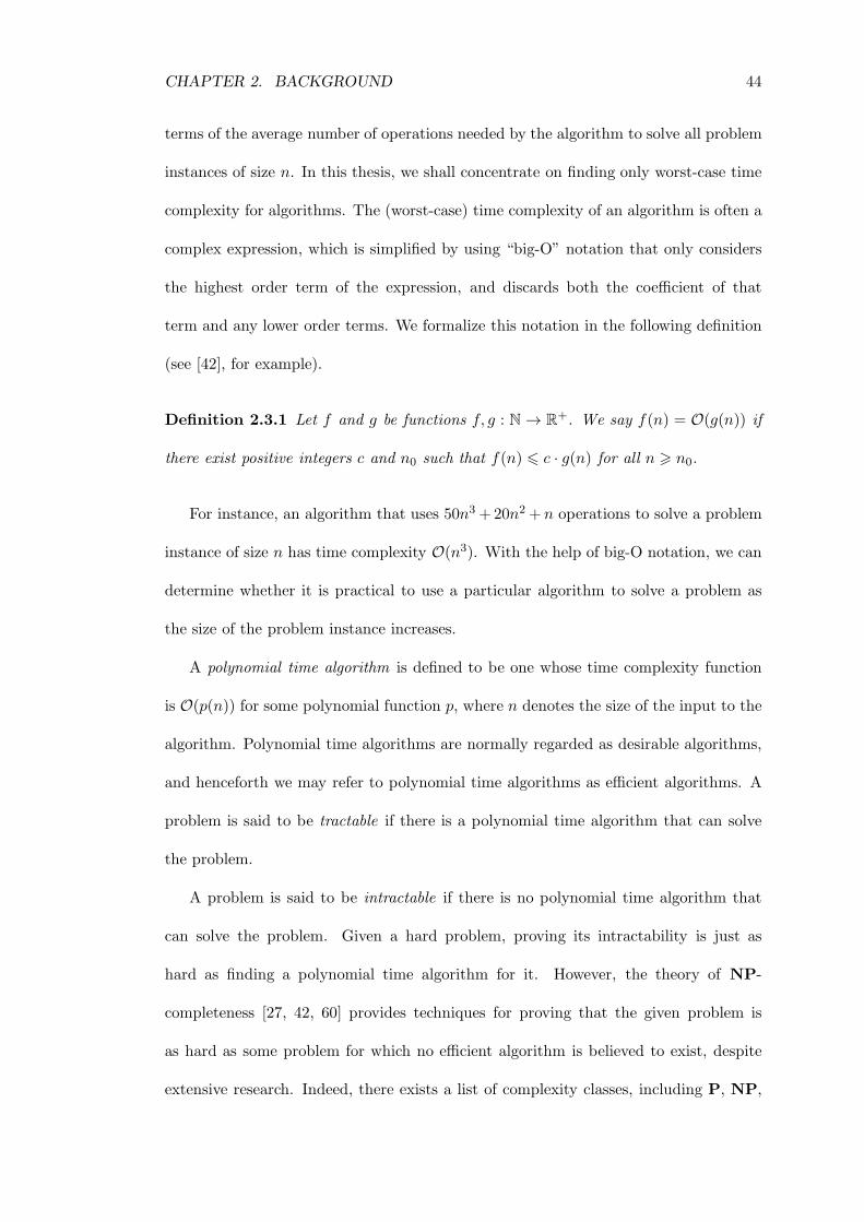
Definition 2.3.1 Let f and g be functions f, g : N → R+. We say f(n) = O(g(n)) if

there exist positive integers c and n0 such that f(n) 6 c · g(n) for all n > n0.

For instance, an algorithm that uses 50n3 +20n2 +n operations to solve a problem

instance of size n has time complexity O(n3). With the help of big-O notation, we can

determine whether it is practical to use a particular algorithm to solve a problem as

the size of the problem instance increases.

A polynomial time algorithm is defined to be one whose time complexity function

is O(p(n)) for some polynomial function p, where n denotes the size of the input to the

algorithm. Polynomial time algorithms are normally regarded as desirable algorithms,

and henceforth we may refer to polynomial time algorithms as efficient algorithms. A

problem is said to be tractable if there is a polynomial time algorithm that can solve

the problem.

A problem is said to be intractable if there is no polynomial time algorithm that

can solve the problem. Given a hard problem, proving its intractability is just as

hard as finding a polynomial time algorithm for it. However, the theory of NP-

completeness [27, 42, 60] provides techniques for proving that the given problem is

as hard as some problem for which no efficient algorithm is believed to exist, despite

extensive research. Indeed, there exists a list of complexity classes, including P, NP,


NP-complete and NP-hard, where each class identifies a set of problems of related

time complexity.

Reduction is a basic tool for relating the time complexities of different problems.

Basically, a reduction from a problem φ to a problem φ′ presents a method for solving

φ using an algorithm for φ′. Before defining two important types of reductions, we

introduce the concept of a decision problem on which the complexity classes P, NP

and NP-complete are based.

We define a decision problem φ to be a predicate φ : Iφ → {0, 1}. In other words,

every instance of the decision problem has one of two solutions. A decision problem φ

is said to be in P if there exists a polynomial time algorithm that solves φ.

In order to define NP we introduce the concept of a nondeterministic algorithm.

A nondeterministic algorithm for a decision problem φ takes a problem instance i ∈

Iφ as input, and executes the following two stages: (i) nondeterministically guess a

structure S (also called certificate) from i, and (ii) verify deterministically whether S

can prove that the answer for i is 1. The algorithm outputs “yes” if there exists S that

proves that the answer for i is 1 and outputs “no” otherwise. The computation of an

nondeterministic algorithm is a tree whose branches correspond to different possible

guesses, and each independent guess is verified concurrently. The time complexity of a

nondeterministic algorithm is defined to be the time used by the longest computation

branch [85], that is the largest number of operations used to verify a particular guess.

A nondeterministic algorithm is said to solve a decision problem φ in polynomial time

if there exists a polynomial p such that, for any problem instance i ∈ Iφ of size n, there

exists at least one guess S which leads the algorithm to return “yes” with the time

complexity O(p(n)) if and only if the answer for i is 1.6 A decision problem φ is said

6Clearly, this definition imposes that the size of the guessed structure S is polynomially bounded,because the algorithm should be able to check that guess in polynomial time.


to be in NP if it can be solved by a polynomial time nondeterministic algorithm.

Consider the set cover problem: given a universe U , a collection C of subsets of U

such that U =⋃

C∈C C, and an integer k, does C contain a cover of U having size k or

less, that is, a subset D ⊆ C such that⋃

D∈DD = U and |D| 6 k? There is no known

polynomial time algorithm for solving the set cover problem. We can easily obtain an

exponential time algorithm for this problem by searching every possible subset of C until

one with the desired property is found. However, we can construct a nondeterministic

algorithm that simply guesses a subset D of C and checks in polynomial time whether

the union of D’s elements equals U and whether D has no more than k elements.

Clearly, for any instance (U, C, k) of the set cover problem, there will exist a guess that

leads the nondeterministic algorithm to produce an output of “yes” if and only if there

exists a cover for the instance (U, C, k). Therefore, the set cover problem is in NP.

The question of whether P = NP is one of the greatest unsolved problems in the-

oretical computer science. It is easy to see that P ⊆ NP, because a deterministic

algorithm is just a special case of a nondeterministic one, in which no guess is per-

formed [42]. However, it is not known whether NP ⊆ P. Most researchers believe that

NP * P, because no polynomial time algorithm has been found for certain problems

in NP such as the set cover decision problem. The concept of NP-completeness is

very useful when considering the question of whether P = NP. Informally, the NP-

complete problems are the “hardest” problems in NP in the sense that they are the

ones most likely not to be in P.

Definition 2.3.2 Given two decision problems φ and φ′, we say there is a polynomial

transformation from φ to φ′ (written φ ∝ φ′) if there is a polynomial time function

f : Iφ → Iφ′ such that for all i ∈ Iφ, φ(i) = 1 if and only if φ′(f(i)) = 1.

A decision problem φ is said to be NP-complete if φ is in NP, and for every


problem φ′ in NP there exists a polynomial transformation of φ′ to φ. Since polynomial

transformation is transitive, we can also say that a decision problem φ isNP-complete if

φ is in NP, and there exists a polynomial transformation from a known NP-complete

problem φ′ to φ. If an NP-complete problem can be solved by a polynomial time

algorithm, then all the problems in NP are tractable. Thus, the question of whether

P = NP is reduced to the question of whether NP-complete problems are tractable.

The techniques for proving NP-completeness can be used to prove the hardness for

some problems outside NP. The basic idea is to generalize the notion of the polynomial

transformation in such a way that a set of problems other than decision problems can

be shown at least as hard as the NP-complete problems.

Definition 2.3.3 An oracle for problem φ is an abstract device that is capable of re-

turning a solution for any instance of φ. It is assumed that the oracle returns the

solution in just one computational step.

Definition 2.3.4 Given two problems φ and φ′, we say

• there is a polynomial time Turing reduction from φ to φ′ (written φ ∝T φ′) if

there is a polynomial time algorithm f which solves φ by querying an oracle for

φ′.

• φ and φ′ are polynomial time Turing equivalent (written φ =T φ′) if φ ∝T φ

′ and

φ′ ∝T φ.

We are not concerned with the way the oracle determines its responses. We can

imagine the oracle for φ′ as a subroutine someone gives to us. We don’t know how

it works, we just know what it returns. What we need to do is to write a program

f to solve φ in polynomial time by invoking the subroutine for φ′ many times in the

program f (though no more than a polynomially bounded number of times). Now we


say that a (general) problem φ is NP-hard if there exists a polynomial time Turing

reduction from a NP-complete problem φ′ to φ. If there is a polynomial time algorithm

for any NP-hard problem, then there are polynomial time algorithms for all problems

in NP, and hence P = NP. Note that, if P = NP, it does not mean that all NP-

hard problems are tractable, because some NP-hard problems may be harder than

NP-complete problems.

However, it is important to prove that the hard problem is NP-complete or NP-

hard, because it provides a better understanding of the problem and leads algorithm

designers to work on productive algorithms. For example, we can stop searching for a

polynomial time algorithm that computes an exact solution to the problem. Instead,

we might look for a heuristic algorithm that runs in polynomial time and computes a

solution that is “close” to the exact one. The quality of a heuristic algorithm is usually

evaluated and compared through empirical experiments [47]. Alternatively, we might

design an approximation algorithm that extends the heuristic algorithm with the worst

case guarantees on the quality of the solution produced by the algorithm [5].

Further detail about the theory of NP-completeness and approximation algorithms

can be found in [5, 42, 91], for example. In Chapter 5 we will use the theory of

NP-completeness to prove the complexity results for some computational problems in

role-based access control, and design a number of heuristic algorithms to solve one of

those problems in Chapter 6.

Chapter 3

The Oriented Permission RBAC

Model and its Applications

Role-based access control and role hierarchies have generated considerable research

activity in recent years. Crampton [29] suggested a role-based access control model that

adopts a similar approach to RBAC96 with respect to the role hierarchy and the user-

role assignment relation, but proposed a new approach to permissions and permission

inheritance within the role hierarchy. In particular, permissions are oriented and can be

inherited in one of three ways within the hierarchy: by more senior roles, by less senior

roles and by no other roles. The motivation for this model is to address the deficiencies

of the standard RBAC approach to inheritance and to offer certain advantages over

existing role-based models. Hereafter we refer to this model as OP-RBAC (Oriented

Permission RBAC).

The main contribution of this chapter is to investigate various applications of OP-

RBAC. Since the introduction of RBAC, several authors have discussed the relationship

between RBAC and the Bell-LaPadula model [69, 72, 73, 81]. Osborn et al [73] show

that information flow policies in a number of different Bell-LaPadula models can be

49

CHAPTER 3. THE OP-RBAC MODEL AND ITS APPLICATIONS 50

implemented in RBAC by the addition of a second role hierarchy and some constraints

on the RBAC relations. However, these approaches are somewhat artificial and limited.

The model for permission inheritance in OP-RBAC provides an alternative way of

implementing these mandatory policies within the context of RBAC. We believe that

this new approach is simpler, more natural, and more flexible than existing work in

this area.

Separation of duty has always been an important consideration in RBAC models.

However, the standard RBAC model is not without its problems in this area. It is

impossible for a user to activate any role that is senior to any pair of roles that appear

in a dynamic separation of duty constraint. Existing work, such as ERBAC96, requires

a distinction to be made between role activation and permission usage hierarchies to

solve this impasse. We will show how to use OP-RBAC to solve this problem without

having to use a second hierarchy.

It has been shown that there are situations where it is useful to distinguish between

role activation and permission usage inheritance [82]. Such a distinction has been made

in both the ERBAC96 model [82] and the GTRBAC model [58], by introducing distinct

role hierarchies. The final contribution of this chapter is to prove that any instance

of the ERBAC96 model can be transformed into an instance of the OP-RBAC model,

which requires a single role hierarchy.

The remainder of this chapter is organized as follows. In the next section, we

formally present OP-RBAC and inter-relationships among the different components of

the model. In Section 3.2, we briefly summarize the Bell-LaPadula model and introduce

its extensions. In Section 3.3, we illustrate how OP-RBAC can be used to implement a

number of different Bell-LaPadula models with the addition and modification of a few

constraints to the basic model. We also discuss related work in this area and compare it

to our approach. In Section 3.4, we consider two other applications of OP-RBAC: one


is to show that dynamic separation of duty constraints can be defined and enforced in a

hierarchical RBAC model; the other is to demonstrate how to implement the ERBAC06

model using OP-RBAC. A preliminary version of this chapter appeared in 2007 [20].

3.1 The OP-RBAC model

The OP-RBAC model is a role-based access control model that contains a novel ap-

proach to permission inheritance. As we shall see, this model offers certain advantages

over existing standard role-based models. We now formally introduce the characteristic

features of OP-RBAC.

We assume the existence of a partially ordered set of roles (R,6), a set of users U

and a user-role assignment relation UA ⊆ U × R. These components are identical to

the ones in RBAC1. We also assume the existence of a set of permissions P and define

the permission-role assignment relation PA ⊆ P ×R.

The distinctive feature in OP-RBAC is that each permission is “oriented” with

respect to inheritance and can be either “up”, “down” or “neutral”. That is, P is the

disjoint union of P+, P− and P 0, where P+ is the set of up permissions, P− is the

set of down permissions and P 0 is the set of neutral permissions. We denote the set

of roles explicitly assigned to p by Roles(p) and the set of roles authorized for p by the

function RolesE : P → 2R, where

RolesE(p) =

↑Roles(p), if p ∈ P+,

↓Roles(p), if p ∈ P−,

Roles(p), if p ∈ P 0.

.

We say that RolesE(p) is the (set of) effective roles for p.


Given a session s in which a set of roles activated Roles(s) ⊆ ↓Roles(u), where

u = User(s), a request by user u to invoke permission p in session s is only granted if

u has activated one of p’s effective roles in s, that is Roles(s) ∩ RolesE(p) 6= ∅. Hence,

RBAC1 is a special case of OP-RBAC in which all permissions are up permissions, that

is, RolesE(p) = ↑Roles(p) for all p.

3.2 The Bell-LaPadula model and extensions

The Bell-LaPadula model (BLP) is probably the most widely known security model

and implements an information flow policy designed to preserve the confidentiality of

information. To meet security requirements in different contexts, several versions of

BLP have been developed, which differ in the use of security functions for labelling

entities, and the definitions of the simple security property and the *-property. We

assume the existence of a set of security functions Λ. A particular version of BLP

chooses a subset of Λ for assigning security levels to subjects and objects, and defines

the simple security property and the *-property with respect to the chosen security

functions.

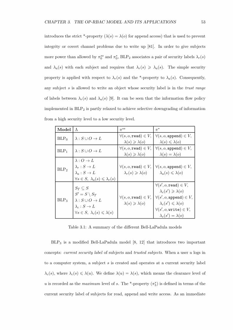
Table 3.1 summarizes the various BLP models in the literature, where πss denotes

the simple security property and π∗ denotes the *-property. We also write πssi to denote

the simple security property in BLPi, and π∗i to denote the *-property in BLPi. Note

that all BLP models include the discretionary security property, which we denote by

πds. It requires that all requests are authorized by the protection matrix M . Recall

that V models the authorizations that have been granted and not yet revoked by the

system. BLP0 corresponds to the simple version of BLP introduced in Chapter 2.

Note that as a consequence of πss0 and π∗0 , a subject s is authorized to write (that

is, simultaneously read and append access) an object o only if λ(s) = λ(o). BLP1


introduces the strict *-property (λ(s) = λ(o) for append access) that is used to prevent

integrity or covert channel problems due to write up [81]. In order to give subjects

more power than allowed by πss0 and π∗0, BLP2 associates a pair of security labels λr(s)

and λa(s) with each subject and requires that λr(s) > λa(s). The simple security

property is applied with respect to λr(s) and the *-property to λa(s). Consequently,

any subject s is allowed to write an object whose security label is in the trust range

of labels between λr(s) and λa(s) [9]. It can be seen that the information flow policy

implemented in BLP2 is partly relaxed to achieve selective downgrading of information

from a high security level to a low security level.

Model Λ πss π∗

BLP0 λ : S ∪O → L∀(s, o, read) ∈ V,

λ(s) > λ(o)

∀(s, o, append) ∈ V,

λ(s) 6 λ(o)

BLP1 λ : S ∪O → L∀(s, o, read) ∈ V,

λ(s) > λ(o)


λ(s) = λ(o)

BLP2

λ : O → L

λr : S → L

λa : S → L

∀s ∈ S, λa(s) 6 λr(s)

∀(s, o, read) ∈ V,

λr(s) > λ(o)


λa(s) 6 λ(o)

BLP3

ST ⊆ S

S′ = S \ STλ : S ∪O → L

λc : S → L

∀s ∈ S, λc(s) 6 λ(s)

∀(s, o, read) ∈ V,

λ(s) > λ(o)

∀(s′, o, read) ∈ V,

λc(s′) > λ(o)

∀(s′, o, append) ∈ V,

λc(s′) 6 λ(o)

∀(s′, o, write) ∈ V,

λc(s′) = λ(o)

Table 3.1: A summary of the different Bell-LaPadula models

BLP3 is a modified Bell-LaPadula model [8, 12] that introduces two important

concepts: current security label of subjects and trusted subjects. When a user u logs in

to a computer system, a subject s is created and operates at a current security label

λc(s), where λc(s) 6 λ(u). We define λ(u) = λ(s), which means the clearance level of

u is recorded as the maximum level of s. The *-property (π∗3) is defined in terms of the

current security label of subjects for read, append and write access. As an immediate


consequence of π∗3 , if a subject is simultaneously reading and appending to two different

objects, the object o that is being appended to will have at least as high a security

label as the object o′ that is being read.

Trusted subjects ST are those subjects not constrained by π∗3. In other words, a

trusted subject is one assumed not to copy high level information into a low level object

even if it is possible [12]. Hence, π∗3 is applied only to untrusted subjects.

On the other hand, the simple security property (πss3 ) is applied to (trusted and

untrusted) subjects S, and is defined with respect to λ(s) for read access. It is worth

noting that given a set of untrusted subjects S′, the satisfaction of π∗3 with respect to

S′ implies the satisfaction of πss3 with respect to S′ [66]. This is because if π∗3 is satisfied

with respect to s′ ∈ S′ then we have λc(s′) > λ(o) for read access, and by definition

λ(s′) > λc(s′).

3.3 Implementing BLP using OP-RBAC

We now demonstrate how, with the addition and subsequent modification of a few

constraints, OP-RBAC can be used to implement the BLP models described in Sec-

tion 3.2. The most important contribution is that OP-RBAC provides a more direct

implementation of the BLP models than has previously been possible using role-based

models [72, 73]. In addition, OP-RBAC supports the assignment of compound permis-

sions (write permissions) which include both read and append access to objects.

We define the state of an OP-RBAC system to be a tuple (W, (UA,RH ,PA)). The

set (UA,RH ,PA) models the access control state, which is used to compute those access

requests that are authorized and would be granted by the access control mechanism.

The set W ⊆ U × P models the set of permissions that are currently “active”; that

is, those permissions that have been granted to users by the access control mechanism.


Initially we ignore πds as it is common to all BLP models. In Section 3.3.7 we discuss

how limited support for πds can be provided in OP-RBAC, unlike existing RBAC

approaches [73], which do not consider this aspect of BLP at all.

3.3.1 Security labels

Crampton [29] discussed why the set of roles assigned to a user can be interpreted as a

security label for that user, while the set of roles assigned to a permission does not have

the same interpretation. We now briefly describe this interpretation, which inspires us

to consider how we might define suitable security labels for users, permissions and

objects in a role-based model.

Let (R,6) be a partially ordered set of roles and let Roles(u) denote the set of

roles explicitly assigned to the user u. Let L(R) = {↓S : S ⊆ R}, then (L(R),⊆) is

the lattice of order ideals in R.1 We can regard ↓Roles(u) in (L(R),⊆) as the actual

security label of u. For example, Figure 3.1 depicts a role hierarchy (R,6) and the

associated lattice (L(R),⊆). If Roles(u) = {r3}, then ↓Roles(u) = {r1, r2, r3} can be

regarded as a security label of u. A user u can activate a session s using some subset

of the roles authorized for u, that is Roles(s) ⊆ ↓Roles(u). We can regard the label

↓Roles(s) in (L(R),⊆) as the current security label of u. For example, a user assigned

to r3 can create a session using role r1, thereby creating a current security label of

{r1}. In short, we interpret the user’s security label in terms of his explicit user-role

assignment(s) in the UA relation, and the user’s current security label in terms of the

roles he has chosen to activate in a session.2 In other words, the user’s security label is

system-defined and the current security label is chosen by the user, which corresponds

closely to λ and λc in BLP3.

1If X is a poset then Y ⊆ X is an order ideal if for all y ∈ Y , x ∈ X, x 6 y implies x ∈ Y .2In actual fact, we associate the sets Roles(u) and Roles(s) with the respective security labels

↓Roles(u) and ↓Roles(s) in L(R).


tr1 tr2

tr3

��

@@@@@

(a) 〈R,6〉

t{r1} t{r2}

t{r1, r2}

t{r1, r2, r3}

t∅

��

@@@@@

@@@@@

��

(b) 〈L(R),⊆〉

Figure 3.1: A role hierarchy and the associated lattice

However, we can not define the security label of a permission in terms of the set of

roles explicitly assigned to the permission, because permission usage in RBAC model is

incompatible with BLP. In RBAC models, permission usage is based on an existential

criterion; a user u is authorized for permission p if there exist roles r and r′ such that

(u, r) ∈ UA, (p, r′) ∈ PA and r′ 6 r. In BLP, permission usage is based on a universal

criterion; a user u is authorized for permission p (to read an object) if the security label

of u dominates the security label of p. In other words, if we interpret the security label of

a permission to be ↓Roles(p), we would require that ↓Roles(p) ⊆ ↓Roles(u). Consider the

following situation: Roles(u) = {r1} and Roles(p) = {r1, r2}. In RBAC, u is authorized

for p, because there exists a role r1 that both u and p are assigned to. However, in

BLP, u is not able to perform p, because ↓Roles(u) = {r1} ⊆ ↓Roles(p) = {r1, r2}.

The incompatibility can be resolved by assigning each permission p to a unique

role r. That is Roles(p) = {r} for some r ∈ R (as is assumed in existing approaches).

In this case, the security label of the permission is ↓r. Moreover, we require that all

permissions for a particular object be assigned to the same role r, thereby the security

label of the object is ↓r.

The limitation of this approach is that we need to construct an additional lattice of


security labels based on the partially ordered set of roles. For each user and permission,

we are also required to map the set of roles associated with the user or the permission

to a security label in the lattice.

An alternative approach is to introduce more restrictive user-role assignment and

permission-role assignment relations in OP-RBAC. We assume that user-role assign-

ment and permission-role assignment are functions, that is, for all u ∈ U and p ∈ P ,

Roles(u) = r and Roles(p) = r′ for some r, r′ ∈ R. Hence, roles r and r′ can be in-

terpreted as the security labels for user u and permission p respectively. Note that

this approach of defining security labels of a user and of a permission is adopted by

most existing work [73, 81], because the simplicity of this approach provides a natural

implementation of BLP models, although it would be a significant restriction in general

RBAC models. Along with this approach, we now demonstrate how OP-RBAC can be

constrained to simulate BLP0, BLP1, BLP2, and BLP3.

3.3.2 BLP0

Recall that a BLP0 system is defined by (L,6) and λ : U ∪O → L. Granted requests

must satisfy πss0 and π∗0 . In order to implement BLP0 using OP-RBAC, we set (R,6)

equal to (L,6). In addition, we define the following constraints:

Constraint 3.3.1 UA is a function; in other words, each user is assigned to a unique

role. The security label of u is defined to be r, where (u, r) ∈ UA.

Constraint 3.3.2 A user u has no choice when running a session; the unique role to

which he is assigned is activated.

Constraint 3.3.3 PA is a function; each permission is assigned to a unique role.

Constraint 3.3.4 Each permission has the form (o,m), where m ∈


{read, append, write} and o is an object. We require that all three permissions

are assigned to the same role r. The security label of o is defined to be r.

Constraint 3.3.5 If p = (o, read) then p ∈ P+.

Constraint 3.3.6 If p = (o, append) then p ∈ P−.

Constraint 3.3.7 If p = (o, write) then p ∈ P 0.

We now prove that given a BLP0 system, we have an OP-RBAC system with

appropriate constraints defined above that is equivalent to the BLP0 system, in the

sense that the same set of requests is authorized.

Theorem 3.3.1 Given a BLP0 system Σ defined by (L,6) and λ, and an OP-RBAC

system Σ′ that satisfies constraints 3.3.1–3.3.7, then a request (u, p) is authorized in Σ

(by satisfying πss0 and π∗0) if and only if (u, p) is authorized in Σ′.

Proof We first prove the “if” condition.

LetW ⊆ U×P be the set of permissions that have been granted to users in the OP-

RBAC system Σ′. Let (u, p) ∈ W , where p = (o, read), (p, r) ∈ PA, and (u, r′) ∈ UA.

By Constraint 3.3.5, we have RolesE(p) = ↑r. Moveover, since (u, p) ∈ W , there exists

a session s activated by u such that Roles(s) ∩ RolesE(p) 6= ∅. By Constraint 3.3.2,

Roles(s) = {r′}. Hence r′ ∈ ↑r; that is r′ > r. By Constraint 3.3.1, λ(u) = r′, and by

Constraint 3.3.4, λ(o) = r; that is λ(u) > λ(o). Hence πss0 is satisfied.

Let (u, p) ∈ W , where p = (o, append), (p, r) ∈ PA, and (u, r′) ∈ UA. By Con-

straint 3.3.6, we have RolesE(p) = ↓r. Moveover, since (u, p) ∈ W , there exists a

session s activated by u such that Roles(s) ∩ RolesE(p) 6= ∅. By Constraint 3.3.2,

Roles(s) = {r′}. Hence r′ ∈ ↓r; that is r′ 6 r. By Constraint 3.3.1, λ(u) = r′, and by

Constraint 3.3.4, λ(o) = r; that is λ(u) 6 λ(o). Hence π∗0 is satisfied.


Let (u, p) ∈ W , where p = (o, write), (p, r) ∈ PA, and (u, r′) ∈ UA. By Con-

straint 3.3.7, we have RolesE(p) = {r}. Moveover, since (u, p) ∈ W , there exists a


Roles(s) = {r′}. Hence r′ = r. By Constraint 3.3.1, λ(u) = r′, and by Constraint 3.3.4,

λ(o) = r; that is λ(u) = λ(o). Hence πss0 and π∗0 are satisfied.

We now prove the “only if” condition.

Let V be the set of requests that have been granted in the BLP0 system Σ. Let

(u, p) ∈ V , where p = (o, read). By πss0 , λ(u) > λ(o). By Constraint 3.3.1, λ(u) =

Roles(u) = r′. By Constraint 3.3.2, u can only activate r′ in a session s, that is

Roles(s) = r′. By Constraint 3.3.4, λ(o) = Roles(p) = r, and by Constraint 3.3.5,

RolesE(p) = ↑Roles(p) = ↑r. Since λ(u) > λ(o), r′ ∈ ↑r. Hence Roles(s)∩RolesE(p) 6= ∅.

Therefore u is authorized for p in Σ′.

Let (u, p) ∈ V , where p = (o, append). By π∗0 , λ(u) 6 λ(o). By Constraint 3.3.1,

λ(u) = Roles(u) = r′. By Constraint 3.3.2, u can only activate r′ in a session s, that

is Roles(s) = r′. By Constraint 3.3.4, λ(o) = Roles(p) = r, and by Constraint 3.3.6,

RolesE(p) = ↓Roles(p) = ↓r. Since λ(u) 6 λ(o), r′ ∈ ↓r. Hence Roles(s)∩RolesE(p) 6= ∅.

Therefore u is authorized for p in Σ′.

Let (u, p) ∈ V , where p = (o, write). By πss0 and π∗0 , λ(u) = λ(o). By Con-

straint 3.3.1, λ(u) = Roles(u) = r′. By Constraint 3.3.2, u can only activate r′ in

a session s, that is Roles(s) = r′. By Constraint 3.3.4, λ(o) = Roles(p) = r, and

by Constraint 3.3.7, RolesE(p) = Roles(p) = r. Since λ(u) = λ(o), r′ = r. Hence

Roles(s) ∩ RolesE(p) 6= ∅. Therefore u is authorized for p in Σ′. �

Remark 3.3.1 Previous work in this area can not deal with write permissions [73, 81],

something we believe detracts significantly from the utility of existing approaches. An

important consequence of Theorem 3.3.1 is that for any write permission to be granted,


the user must have exactly the same security label as the object. In other words, our

approach deals with write permissions appropriately, and in the manner intended by the

original BLP model. For this reason alone, we believe our approach is to be preferred

to existing work in the literature.

3.3.3 BLP1

The use of the strict *-property in BLP1 requires a simple modification to Con-

straint 3.3.6.

Constraint 3.3.8 If p = (o, append) then p ∈ P 0.

By Constraint 3.3.8, a user is allowed to perform an append permission only if

the user has activated the role to which the append permission is assigned. This is

analogous to the strict *-property in BLP1 where a user must have the same security

label as an object in order to append to it.

Theorem 3.3.2 Given a BLP1 system Σ defined by (L,6) and λ, and an OP-RBAC

system Σ′ that satisfies constraints 3.3.1–3.3.5 and 3.3.7–3.3.8, then a request (u, p) is

authorized in Σ (by satisfying πss1 and π∗1) if and only if (u, p) is authorized in Σ′.

The proof of this result is similar to that of Theorem 3.3.1 and is omitted.

3.3.4 BLP2

In the trusted network interpretation of multi-level security (BLP2), each user is as-

sociated with a pair of security labels λr(u) and λa(u), where λa(u) 6 λr(u). The

simple security property πss2 is applied with respect to λr(u) and the *-property π∗2

with respect to λa(u). As a consequence, the user can invoke a write permission on an

object whose security label is contained in the range [λa(u), λr(u)]. Clearly, BLP0 is a


subcase of BLP2, where λr(u) = λa(u). To implement BLP2 in OP-RBAC, we replace

Constraints 3.3.1 and 3.3.2 with the following constraints.

Constraint 3.3.9 Each user u is assigned to at most two roles ra and rr with ra 6 rr.

That is Roles(u) = {ra, rr}, where rr corresponds to λr(u) and ra corresponds to λa(u).

Constraint 3.3.10 A user assigned to roles ra and rr has no choice when running a

session; the roles in [ra, rr] are activated.

Theorem 3.3.3 Given a BLP2 system Σ defined by (L,6), λr, λa and λ, and an OP-

RBAC system Σ′ that satisfies constraints 3.3.3–3.3.7 and 3.3.9–3.3.10, then a request

(u, p) is authorized in Σ (by satisfying πss2 and π∗2) if and only if (u, p) is authorized in

Σ′.


Let (u, p) ∈ W , where p = (o, read), (p, r) ∈ PA, (u, rr) ∈ UA, and (u, ra) ∈ UA.

By Constraint 3.3.5, we have RolesE(p) = ↑r. Moveover, since (u, p) ∈ W , there exits

a session s activated by u such that Roles(s) ∩ RolesE(p) 6= ∅; that is, there exists

r′ ∈ Roles(s) such that r′ > r. By Constraint 3.3.10, rr > r′ > ra; that is rr > r. By

Constraint 3.3.9, λr(u) = rr, and by Constraint 3.3.4, λ(o) = r; that is λr(u) > λ(o).

Hence πss2 is satisfied.

Let (u, p) ∈W , where p = (o, append), (p, r) ∈ PA, (u, rr) ∈ UA, and (u, ra) ∈ UA.

By Constraint 3.3.6, we have RolesE(p) = ↓r. Moveover, since (u, p) ∈ W , there exits


r′ ∈ Roles(s) such that r′ 6 r. By Constraint 3.3.10, ra 6 r′ 6 rr; that is ra 6 r. By

Constraint 3.3.9, λa(u) = ra, and by Constraint 3.3.4, λ(o) = r; that is λa(u) 6 λ(o).

Hence π∗2 is satisfied.

Let (u, p) ∈ W , where p = (o, write), (p, r) ∈ PA, (u, rr) ∈ UA, and (u, ra) ∈ UA.

By Constraint 3.3.7, we have RolesE(p) = {r}. Moveover, since (u, p) ∈W , there exits



r′ ∈ Roles(s) such that r′ = r. By Constraint 3.3.10, ra 6 r′ 6 rr, by Constraint 3.3.9,

λr(u) = rr and λa(u) = ra, and by Constraint 3.3.4, λ(o) = r; that is λa(u) 6 λ(o) 6

λr(u). Hence πss2 and π∗2 are satisfied.



(u, p) ∈ V , where p = (o, read). By πss2 , λr(u) > λ(o). By Constraint 3.3.9, λr(u) =

rr ∈ Roles(u). By Constraint 3.3.10, u must activate a set of roles including rr in a

session s, that is rr ∈ Roles(s). By Constraint 3.3.4, λ(o) = Roles(p) = r, and by

Constraint 3.3.5, RolesE(p) = ↑Roles(p) = ↑r. Since λr(u) > λ(o), rr ∈ ↑r. Hence

Roles(s) ∩ RolesE(p) 6= ∅. Therefore u is authorized for p in Σ′.

Let (u, p) ∈ V , where p = (o, append). By π∗2, λa(u) 6 λ(o). By Constraint 3.3.9,

λa(u) = ra ∈ Roles(u). By Constraint 3.3.10, u must activate a set of roles including

ra in a session s, that is ra ∈ Roles(s). By Constraint 3.3.4, λ(o) = Roles(p) = r, and

by Constraint 3.3.6, RolesE(p) = ↓Roles(p) = ↓r. Since λa(u) 6 λ(o), ra ∈ ↓r. Hence


Let (u, p) ∈ V , where p = (o, write). By πss2 and π∗2 , λa(u) 6 λ(o) 6 λr(u).

By Constraint 3.3.9, Roles(u) = {rr, ra}, where rr = λr(u) and ra = λa(u). By

Constraint 3.3.10, u must activate all roles [ra, rr] in a session s, that is Roles(s) =

[ra, rr]. By Constraint 3.3.4, λ(o) = Roles(p) = r, and by Constraint 3.3.7, RolesE(p) =

Roles(p) = r. Since λa(u) 6 λ(o) 6 λr(u), r ∈ [ra, rr]. Hence Roles(s) ∩ RolesE(p) 6= ∅.

Therefore u is authorized for p in Σ′. �


3.3.5 BLP3

BLP3 introduces the current security function λc to simplify the evaluation of the *-

property π∗33, and to improve usability by allowing a user to downgrade his security

level. In addition, BLP3 introduces trusted subjects that are allowed to operate without

the extra encumbrance of π∗3. Typical examples of trusted subjects in the context of

operating systems are device drivers and memory management software.

In order to provide close correlations between BLP3 and OP-RBAC, from now on,

we assume that no subject in BLP3 could be trusted not to copy high level information

into low level objects. In other words, all subjects in BLP3 are untrusted subjects

who subject to πss3 and π∗3 . In this case, as we discussed in Section 3.2, π∗3 implies

πss3 . Hence, a request from a subject to access an object is granted in a BLP3 system

only if this request satisfies π∗3 . In order to implement BLP3 in OP-RBAC, we replace

Constraint 3.3.2 with the following constraint.

Constraint 3.3.11 Each user u can only activate a single role r′ ∈ ↓Roles(u) = ↓r

when running a session s. The current security label of u is defined to be Roles(s) = {r′}

for some r′ 6 r.

Theorem 3.3.4 Given a BLP3 system Σ defined by (L,6), λc, and λ, and an OP-

RBAC system Σ′ that satisfies constraints 3.3.1, 3.3.3–3.3.7 and 3.3.11, then a request

(u, p) is authorized in Σ (by satisfying π∗3) if and only if (u, p) is authorized in Σ′.


Let (u, p) ∈ W , where p = (o, read), (p, r) ∈ PA, and (u, r′) ∈ UA. By Con-

straint 3.3.5, we have RolesE(p) = ↑r. Moveover, since (u, p) ∈ W , there exists a


3The *-property in the earlier formulation of the Bell-LaPadula model [10, 11] requires that thedecision whether to grant a request from a subject to write an object, for example, can only be madeby considering the security labels of all objects the subject has previously read.


Roles(s) = {r′′}. Hence r′′ ∈ ↑r; that is r′′ > r. By Constraint 3.3.11, λc(u) = r′′, and

by Constraint 3.3.4, λ(o) = r; that is λc(u) > λ(o). By Constraint 3.3.1, λ(u) = r′,

and by Constraint 3.3.11, r′′ 6 r′; that is λc(u) 6 λ(u). Hence the first part of π∗3 is

satisfied.

Let (u, p) ∈ W , where p = (o, append), (p, r) ∈ PA, and (u, r′) ∈ UA. By Con-

straint 3.3.6, we have RolesE(p) = ↓r. Moveover, since (u, p) ∈ W , there exists a


Roles(s) = {r′′}. Hence r′′ ∈ ↓r; that is r′′ 6 r. By Constraint 3.3.11, λc(u) = r′′,

and by Constraint 3.3.4, λ(o) = r; that is λc(u) 6 λ(o). Obviously, r′′ 6 r′, hence

λc(u) 6 λ(u). Hence the second part of π∗3 is satisfied.

Let (u, p) ∈ W , where p = (o, write), (p, r) ∈ PA, and (u, r′) ∈ UA. By Con-

straint 3.3.7, we have RolesE(p) = {r}. Moveover, since (u, p) ∈ W , there exists a


Roles(s) = {r′′}. Hence r′′ = r. By Constraint 3.3.11, λc(u) = r′′, and by Con-

straint 3.3.4, λ(o) = r; that is λc(u) = λ(o). Obviously, r′′ 6 r′, hence λc(u) 6 λ(u).

Hence the third part of π∗3 is satisfied.



(u, p) ∈ V , where p = (o, read). By π∗3 , λ(o) 6 λc(u), and λc(u) 6 λ(u). By

Constraint 3.3.1, λ(u) = Roles(u) = r′. By Constraint 3.3.11, u can only acti-

vate a role r′′ in a session s, that is λc(u) = Roles(s) = r′′, where r′′ 6 r′ corre-

sponds to λc(u) 6 λ(u). By Constraint 3.3.4, λ(o) = Roles(p) = r, and by Con-

straint 3.3.5, RolesE(p) = ↑Roles(p) = ↑r. Since λc(u) > λ(o), r′′ ∈ ↑r. Hence


Let (u, p) ∈ V , where p = (o, append). By π∗3 , λc(u) 6 λ(o), and λc(u) 6 λ(u).

By Constraint 3.3.1, λ(u) = Roles(u) = r′. By Constraint 3.3.11, u can only activate


a role r′′ in a session s, that is λc(u) = Roles(s) = r′′, where r′′ 6 r′ corresponds to

λc(u) 6 λ(u). By Constraint 3.3.4, λ(o) = Roles(p) = r, and by Constraint 3.3.6,

RolesE(p) = ↓Roles(p) = ↓r. Since λc(u) 6 λ(o), r′′ ∈ ↓r. Hence Roles(s)∩RolesE(p) 6=

∅. Therefore u is authorized for p in Σ′.

Let (u, p) ∈ V , where p = (o, write). By π∗3, λc(u) = λ(o) and λc(u) 6 λ(u). By

Constraint 3.3.1, λ(u) = Roles(u) = r′. By Constraint 3.3.11, u can only activate a

role r′′ in a session s, that is λc(u) = Roles(s) = r′′, where r′′ 6 r′ corresponds to

λc(u) 6 λ(u). By Constraint 3.3.4, λ(o) = Roles(p) = r, and by Constraint 3.3.7,

RolesE(p) = Roles(p) = r. Since λc(u) = λ(o), r′′ = r. Hence Roles(s) ∩ RolesE(p) 6= ∅.

Therefore u is authorized for p in Σ′. �

3.3.6 BLP4

A further extension of BLP0, which we call BLP4, associates each object with two

different security labels, λr(o) and λa(o); πss4 is defined using λr(o) and π∗4 is defined

using λa(o). We might require, by analogy with BLP2, that the “append-level” of an

object is higher than the “read-level”; that is λa(o) > λr(o). In this case, a subject

whose security label is contained in the range [λr(o), λa(o)] can have write access to

the object. This is the analogue of the trusted range of subjects in the trusted network

interpretation (BLP2).

However, note that we can support some useful access control policies if we drop

the requirement that λa(o) > λr(o), in which case no user can both read and append

(write) that object o. Consider an object such as an audit log file f : we require that

low level users must append to f , while high level users can read f but must not to be

able change it. We can implement these requirements simply by making λa(f) < λr(f).

Hence, in BLP4, we do not insist that λr(o) 6 λa(o). Table 3.2 summarizes BLP4.

To implement BLP4 in OP-RBAC, we replace Constraints 3.3.3 and 3.3.4 with the


Model Λ πss π∗

BLP4

λ : S → L

λr : O → L

λa : O → L

∀(s, o, read) ∈ V,

λ(s) > λr(o)


λ(s) 6 λa(o)

Table 3.2: BLP4

following constraint.

Constraint 3.3.12 If p = (o,m), where m ∈ {read, append}, p is assigned to a unique

role, but permissions for the same object, (o, read) and (o, append), may be assigned to

different roles. The assignment of a write permission for the same object, (o, write),

depends on the ordering between roles to which (o, read) and (o, append) are assigned.

More specifically, for each object o such that ((o, read), rr), ((o, append), ra) ∈ PA, the

permission (o, write) should assigned to all roles in [rr, ra] if rr 6 ra. In the case that

rr ra, this permission can not be assigned to any role. Hence, rr corresponds to λr(o)

and ra corresponds to λa(o).

Theorem 3.3.5 Given a BLP4 system Σ defined by (L,6), λr, λa and λ, and an OP-

RBAC system Σ′ that satisfies constraints 3.3.1, 3.3.2, 3.3.5–3.3.7, and 3.3.12, then

a request (u, p) is authorized in Σ (by satisfying πss4 and π∗4) if and only if (u, p) is

authorized in Σ′.


Let (u, p) ∈ W , where p = (o, read), (p, rr) ∈ PA, and (u, r) ∈ UA. By Con-

straint 3.3.5, we have RolesE(p) = ↑rr. Moveover, since (u, p) ∈ W , there exists a


Roles(s) = {r}. Hence r ∈ ↑rr; that is r > rr. By Constraint 3.3.1, λ(u) = r, and by

Constraint 3.3.12, λr(o) = rr; that is λ(u) > λr(o). Hence πss4 is satisfied.

Let (u, p) ∈ W , where p = (o, append), (p, ra) ∈ PA, and (u, r) ∈ UA. By Con-

straint 3.3.6, we have RolesE(p) = ↓ra. Moveover, since (u, p) ∈ W , there exists a



Roles(s) = {r}. Hence r ∈ ↓ra; that is r 6 ra. By Constraint 3.3.1, λ(u) = r, and by

Constraint 3.3.12, λa(o) = ra; that is λ(u) 6 λa(o). Hence π∗4 is satisfied.

Let (u, p) ∈ W , where p = (o, write) and (u, r) ∈ UA. Let

((o, read), rr), ((o, append), ra) ∈ PA. By Constraint 3.3.12, Roles(p) = [rr, ra]. By

Constraint 3.3.7, we have RolesE(p) = Roles(p) = [rr, ra]. Moveover, since (u, p) ∈ W ,

there exists a session s activated by u such that Roles(s) ∩ RolesE(p) 6= ∅. By Con-

straint 3.3.2, Roles(s) = {r}. Hence r ∈ [rr, ra]. By Constraint 3.3.1, λ(u) = r, and by

Constraint 3.3.12, λr(o) = rr, λa(o) = ra; that is λr(o) 6 λ(u) 6 λa(o). Hence πss4 and

π∗4 are satisfied.



(u, p) ∈ V , where p = (o, read). By πss4 , λ(u) > λr(o). By Constraint 3.3.1, λ(u) =

Roles(u) = r′. By Constraint 3.3.2, u can only activate r′ in a session s, that is

Roles(s) = r′. By Constraint 3.3.12, λr(o) = Roles(p) = rr, and by Constraint 3.3.5,

RolesE(p) = ↑Roles(p) = ↑rr. Since λ(u) > λr(o), r′ ∈ ↑rr. Hence Roles(s)∩RolesE(p) 6=

∅. Therefore u is authorized for p in Σ′.

Let (u, p) ∈ V , where p = (o, append). By π∗4, λ(u) 6 λa(o). By Constraint 3.3.1,

λ(u) = Roles(u) = r′. By Constraint 3.3.2, u can only activate r′ in a session s,

that is Roles(s) = r′. By Constraint 3.3.12, λa(o) = Roles(p) = ra, and by Con-

straint 3.3.6, RolesE(p) = ↓Roles(p) = ↓ra. Since λ(u) 6 λa(o), r′ ∈ ↓ra. Hence


Let (u, p) ∈ V , where p = (o, write). By πss4 and π∗4, λr(o) 6 λ(u) 6 λa(o). By

Constraint 3.3.1, λ(u) = Roles(u) = r′. By Constraint 3.3.2, u can only activate r′

in a session s, that is Roles(s) = r′. By Constraint 3.3.12, λr(o) = rr and λa(o) =

ra. Since rr 6 ra, by Constraint 3.3.12, Roles(p) = [rr, ra]. By Constraint 3.3.7,


RolesE(p) = Roles(p) = [rr, ra]. Since λr(o) 6 λ(u) 6 λa(o), Roles(s) ∈ [rr, ra]. Hence

Roles(s) ∩ RolesE(p) 6= ∅. Therefore u is authorized for p in Σ′. �

3.3.7 The discretionary security property

An information flow policy authorizes access purely on the basis of the labelling of the

subject and object. For example, a subject s is authorized to append to an object o

only if λ(s) 6 λ(o). However, in many situations, it will be undesirable for a user to

append to a file with a higher security label. The protection matrix is usually used

to augment the information flow policy when defining authorization requirements in

computer systems. We might enforce the above requirement in BLP simply by ensuring

that append 6∈Ms,o.

Existing work on implementing BLP using RBAC ignores the discretionary prop-

erty [29, 69, 72, 73, 81], meaning that the range of policies that can be implemented

are somewhat limited. We now show that it is at least possible to implement some

coarse-grained discretionary properties using OP-RBAC.

Suppose that we do not wish users with security label r to be able to append

to objects with security label r′ > r. Constraint 3.3.6 insists that (o, append) is a

down permission. Instead the administrator can define this permission to be a neutral

permission, so that only users with security label r′ can append to o. Of course, the

administrator can also assign this neutral permission to other roles r′′ 6 r′ if desired. In

other words, making certain permissions neutral rather than up or down, gives limited

support for policies defined at the administrator’s discretion. To support discretionary

security we replace Constraints 3.3.5 and 3.3.6 with the following constraints.

Constraint 3.3.13 If p = (o, read) and (p, r) ∈ PA, then either p ∈ P+ or p ∈ P 0

and RolesE(p) ⊆ ↑r.


Constraint 3.3.14 If p = (o, append) and (p, r) ∈ PA, then either p ∈ P− or p ∈ P 0

and RolesE(p) ⊆ ↓r.

There is one distinct limitation to this approach. Namely, we cannot define our

policies at the user-level, only at the role-level. This means that it is not possible

to achieve the granularity of policy specification that is available in the BLP model

via the protection matrix.4 This is an inherent limitation of the RBAC paradigm,

not the OP-RBAC model. One advantage of this approach over BLP is that policy

specification is much more economical. This, of course, is one of the advantages of the

RBAC paradigm. It is instructive to note that OP-RBAC can support this level of

discretionary policy specification, while standard RBAC cannot.

3.3.8 Discussion

There have been several attempts to implement BLP models using role-based mod-

els [29, 69, 72, 73, 81]. Osborn et al ’s approach [69, 72, 73] shows how the role-graph

model can be configured to enforce information flow policies.

In their approach the lattice of security labels is defined separately and indepen-

dently from the role graph. Each subject and object is assigned a security label, as in

BLP. Then the r-level of a role r, denoted by r-level(r), is defined to be the least upper

bound of the security labels of the objects for which (o, read) is in the permissions of

the role r; and the a-level of a role r, denoted by a-level(r), is the greatest lower bound

of the security labels of the objects for which (o, append) is in the permissions of the

role r. For all (u, r) ∈ UA, the security level of a user u must be greater than or equal

to the r-level of r, and for all (u, r) ∈ UA, the security level of a user u must be less

than or equal to the a-level of r.

4In fact our approach is equivalent to a BLP model in which the protection matrix has rows indexedby security levels and columns indexed by objects.


It has been noted that this approach creates a permission-permission conflict [88].

For example, a role r contains permissions to objects labeled with security labels

(rts, as), where rts denotes “read top secret” and as denotes “append secret”; that

is, r-level(r) is rts and a-level(r) is as. Therefore, the role r cannot be assigned to

any user without violating information flow policies. In addition, we think their ap-

proach for simulating the basic information flow policy using role-based access control

is complicated, because their approach needs to introduce an extra lattice structure

to determine the security labels of users and objects, and requires modification to the

role-graph algorithms to compute the r-level and a-level of each role in the role graph

model.

An alternative approach was developed by Sandhu et al [73, 81]. They introduced

two partial orderings, 6r and 6a, on the set of roles. This gives rise to two hierarchies

RH r and RH a, one for read roles and one for append roles. The append hierarchy

RH a is the dual of the read hierarchy RH r: that is, x 6 y in the append hierarchy

if and only if x > y in the read hierarchy. Figure 3.2 shows a simple example of the

read hierarchy and the corresponding append hierarchy. We write xr for role x in the

read hierarchy and xa for the corresponding role in the append hierarchy. Each pair

of permissions (o, read) and (o, append) is assigned to exactly one matching pair of xr

and xa roles in RH r and RH a respectively. Thereby, the security label of object o is

implicitly defined to be x.

A number of constraints, similar to a number of ours were also defined. Note

that, in BLP, every subject has a unique security label, and the concept of subjects

corresponds to sessions in RBAC96 [83]. Hence, they require that each session has

exactly two matching roles yr and ya. A read permission is granted if yr > xr in RH r

and an append permission is granted if ya > xa in RH a. Since RH a is the dual of RH r,

the condition of granting an append permission is actually ya 6 xa in original lattice


tbr tcr

tdr

tar

��

@@@@@

@@@@@

��

(a) RH r

tba tca

taa

tda

��

@@@@@

@@@@@

��

(b) RH a

Figure 3.2: A read hierarchy and the corresponding append hierarchy

structure. We think it is not necessary to use a second hierarchy. More importantly,

this approach can not cope with a compound (write) permission that has both read

and append access rights to an object and does not consider discretionary aspects of

the BLP model. Finally, the simulation of BLP3 is not covered in their approach.

Crampton recently introduced the OP-RBAC model, and illustrated how OP-RBAC

can be used to implement multi-level secure systems with the addition of few constraints

to the basic model. The constrained OP-RBAC model simulates a more “general”

version of BLP, where the read permission p = (o, read) and the append permission

p′ = (o, append) are assigned to the unique roles rr and ra respectively, and the security

label of an object λ(o) is defined to be a range [rr, ra]. Clearly, there are a number of

possibilities for the security label of an object: if rr = ra, λ(o) = rr = ra; if rr < ra,

λ(o) = [rr, ra]; if ra < rr, λ(o) = ∅. However, in the standard BLP models, the security

label of an object is unique, which corresponds to the situation where rr = ra. On the

other hand, it is rare to see any BLP models with the security label of an object being

either ∅ or [rr, ra], which makes it difficult to compare the security label of an object

with the security label of a subject. In other words, the constrained OP-RBAC model

only implements a simple version of BLP, that is, BLP0.

We re-examined OP-RBAC, with the addition and modification of a few constraints,

to provide greater correlation between role-based and mandatory access control. Com-


pared with previous attempts, our approach provides a more direct implementation of a

number of different BLP models. We do not require an additional hierarchy and are able

to support the assignment of “mixed” permissions (write permissions), which include

both read and append access to objects. In addition, our approach provides a natural

implementation of BLP3 in terms of untrusted subjects, which has not been studied in

most existing work. Perhaps the most significant contribution of the OP-RBAC model

is the support for some limited discretionary policies, something existing work does not

consider and would be ill-equipped to implement. Furthermore, we introduce BLP4,

an additional BLP model, that may provide some useful features unavailable in other

BLP models. We have shown that BLP4 can also be implemented in OP-RBAC.

3.4 Other applications

In this section, we show how OP-RBAC can be used to remove some of the problems

associated with the integration of role hierarchies and separation of duty requirements.

We also investigate how to distinguish role activation and permission inheritance in a

single OP-RBAC hierarchy.

3.4.1 Separation of duty

Separation of duty is widely considered to be a fundamental principle in computer

security [25, 77]. In its simplest form, the principle requires that if a sensitive task

comprises two steps, then the same user can not perform both steps. A typical example

of separation of duty for a purchase order application is the requirement that creating

(p) and approving (q) a purchase order can not be performed by the same user.

Separation of duty has always been an important consideration in role-based access

control models. An approach commonly advocated in standard RBAC is to define


constraints on the authorizations of users to roles to ensure that no users can invoke

both permissions p and q. This may be done through appropriate configuration of

the UA relation (so called static separation of duty), or by limiting the roles that

can be activated by users in a single session (dynamic separation of duty). Dynamic

separation of duty is claimed to provide greater operational flexibility in practice [2].

Assume that p and q are assigned to roles r1 and r2 respectively, dynamic separation

of duty requires that no user is permitted to activate both r1 and r2 in the course of

any session, although it is possible for a user to be assigned to both roles. However, as

we noted in Chapter 2, the role hierarchy may be incompatible with the enforcement of

dynamic separation of duty constraints. That is, it is not possible to have a role r that

is more senior than two roles r1 and r2 which are in dynamic separation of duty [62].

More specifically, assume that there exists some users who are able to activate roles r1

and r2 in different sessions, there is no means to assign these users to a common senior

role r because activation of role r violates dynamic separation of duty with respect to

r1 and r2. Therefore, these common users have to be explicitly assigned to roles r1 and

r2, which goes against the idea of a role hierarchy to reduce administrative complexity.

OP-RBAC introduced three different types of permissions and proposed a new

mechanism for permission inheritance within a role hierarchy. This new approach of

permission inheritance in OP-RBAC makes it possible to implement dynamic separa-

tion of duty constraints on two roles that have a common senior role and for a user to be

assigned to or activate the senior role. The basic idea is to define sensitive permissions

to be different types of permissions so that these permissions can not be aggregated

to a single role. Formally, we require that RolesE(p) ∩ RolesE(q) = ∅, which means

no single role is authorized for both permissions p and q. Note that this condition

does not exclude the case that there exists a role that is more senior than two roles

to which sensitive permissions p and q are explicitly assigned, and this senior role can


be activated by a user without violating dynamic separation of duty constraints on its

junior roles.

Figure 3.3 illustrates the seven ways of ensuring that for mutually exclusive permis-

sions p and q assigned to roles r1 and r2 respectively, RolesE(p) ∩ RolesE(q) = ∅. (The

roles enclosed by a curve illustrate the effective set of roles for each permission.) The

most obvious solution is to make p and q neutral permissions and assign them to roles

r1 and r2 respectively, as shown in Figure 3.3(a). Therefore, u can be assigned to the

more senior role r and activate r without acquiring the mutually exclusive permissions

p and q. In addition, Figures 3.3(b)–3.3(g) shows that it is possible for u to be assigned

to senior roles r or r′ by defining p and q to be other types of permissions.

tr′@@@@tr1

��tr2@

@@@

��tr

��

��

(a) p, q ∈ P 0

tr′@@@@tr1

��tr2@

@@@

��tr

��

....................

........

...

.....

.

..

..

.

..

.

.

..

.

..

.

..

.

.

..

...

..

..

..

..

..

.

.

...

..

...

...

..

...

...

...

............

..

.................

.

....................

.....................

...................

..................

.................

................

....................

..

..

....

..

.

..

..

.

.

..

..

.

..

.

.

..

.

..

.

..

.

.

..

..

..

.

..

..

..

..

.

.

..

.

..

..

.

..

.

..

..

.

..

.

..

.

..

.

..

..

..

.

..

..

..

..

..

..

..

..

..

..

.

.

..

..

..

..

..

..

..

..

..

..

..

..

..

..

.............

...................

..................

.................

................

(b) p ∈ P+, q ∈ P 0

tr′@@@@tr1

��tr2@

@@@

��tr

��

................

.................

..................

...................

.....................

.....................

..

.................

...

...............

.

...

...

..

...

..

...

..

..

..

..

..

...

..

.

..

.

..

.

..

.

..

..

..

..

.

..

........

........

......... ...........

................

.................

..................

..

.................

..

..

.................

..

..

..

..

.

..

..

..

..

..

..

..

..

..

..

..

..

..

..

..

.

..

.

..

.

..

..

..

.

..

.

..

.

..

.

..

..

.

..

.

..

..

.

..

..

..

..

..

..

.

..

.

..

.

..

.

..

.

..

..

..

.

..

..

..

..

..

.

.

..

......

....................

(c) p ∈ P 0, q ∈ P+

tr′@@@@tr1

��tr2@

@@@

��tr

��

................

.................

..................

...................

.....................

.....................

.

..................

...

...

............

.

..

...

...

..

...

...

.

...

..

..

..

..

..

..

.

..

.

..

.

..

..

..

.

..

..

..

........

........

....................

................

.................

..................

..

.................

..

..

..

...............

..

..

..

..

..

.

..

..

..

..

..

..

.

..

..

..

..

..

..

..

..

.

..

.

..

.

..

.

..

..

..

.

.

..

..

..

.

..

.

..

..

.

..

.

..

..

..

..

..

..

..

.

..

.

..

.

..

.

.

.

..

..

..

..

.

..

..

..

..

..

......

....................

(d) p ∈ P−, q ∈ P 0

tr′@@@@tr1

��tr2@

@@@

��tr

��

....................

........

.

.......

.

..

.

..

..

.

..

..

..

.

..

.

.

..

..

..

..

..

..

..

..

.

..

...

...

..

...

...

..

................

.

..................

.....................

.....................

...................

..................

.................

................

....................

..

......

..

..

..

..

.

..

..

..

.

.

.

..

..

.

..

.

..

..

.

..

..

..

..

..

.

..

..

..

..

.

..

.

..

..

.

..

..

.

..

..

..

.

..

.

..

..

.

..

.

..

..

..

..

..

..

..

..

..

.

..

..

..

..

..

..

..

..

..

..

..

..

..

.............

...................

..

................

.................

................

(e) p ∈ P 0, q ∈ P−

tr′@@@@tr1

��tr2@

@@@

��tr

....................

........

..

......

.

..

.

..

..

.

.

..

.

..

.

..

.

.

..

..

..

...

..

..

..

.

.

...

..

...

..

...

...

...

...............

..

.................

.....................

.....................

...................

..................

.................

................

....................

..

......

..

..

..

..

.

..

..

..

.

.

.

..

.

..

.

..

..

..

..

.

..

..

..

..

..

.

.

..

.

..

.

..

..

.

..

.

..

..

.

..

..

..

.

..

.

..

.

..

..

..

..

..

..

.

..

..

..

..

..

..

..

..

..

..

..

..

..

..

.

..

..

.................

...................

..................

.................

................

....................

........

.

.......

.

..

.

..

..

.

..

..

..

.

..

.

.

..

..

..

..

..

..

..

..

.

..

...

...

..

...

...

..

................

.

..................

.....................

.....................

...................

..................

.................

................

....................

........

..

..

..

..

.

..

..

..

.

.

.

..

..

.

..

.

..

..

.

..

..

..

..

..

.

..

..

..

..

.

..

.

..

..

.

..

..

.

..

..

..

.

..

.

..

..

.

..

.

..

..

..

..

..

..

..

..

..

.

..

..

..

..

..

..

..

..

..

..

..

.................

..

..

...............

..................

.................

................

(f) p ∈ P+, q ∈ P−

tr′@@@@tr1

��tr2@

@@@

��tr

................

.................

..................

...................

.....................

.....................

.

..................

...

...

............

.

..

...

...

..

...

...

.

..

...

..

..

..

..

..

.

..

.

..

.

..

.

.

..

.

..

..

..

........

........

....................

................

.................

..................

...................

..

..

..

..

.............

..

..

..

..

..

..

..

..

..

..

.

..

.

..

..

..

..

..

..

..

..

.

..

.

..

.

..

.

..

..

..

.

.

..

..

..

.

..

.

..

..

.

..

..

..

..

.

..

..

..

..

.

..

.

..

..

.

..

.

.

.

..

..

..

.

..

..

..

..

..

......

....................

................

.................

..................

...................

.....................

.....................

.

..................

..

................

...

...

..

...

...

..

.

.

..

..

...

..

..

..

..

.

..

.

..

.

..

.

.

.

..

..

..

..

........

........

....................

................

.................

..................

..

.................

..

..

..

...............

..

..

..

..

..

..

..

..

..

..

.

..

.

..

..

..

..

..

..

..

..

.

..

.

..

.

..

..

..

.

..

.

.

..

..

.

..

..

.

..

..

.

..

.

..

..

..

..

..

..

..

.

.

.

..

.

..

..

.

.

.

.

..

..

..

.

..

..

..

..

........

....................

(g) p ∈ P−, q ∈ P+

Figure 3.3: Implementing separation of duty using different types of permissions

Of course, we still need to define dynamic separation of duty constraints in OP-


RBAC to prevent, for example, u from activating roles r1 and r2 in the same session.5

Formally, we require that for all u ∈ U , either Roles(s) ∩ RolesE(p) = ∅ or Roles(s) ∩

RolesE(q) = ∅, where u = User(s). This conditions means that no user is allowed

to activate a set of roles to which mutually exclusive permissions are assigned in any

session.

3.4.2 Usage and activation hierarchies

In most RBAC models, the role hierarchy serves two distinct purposes.

• A role is assumed to inherit the permissions assigned to roles below it in the

hierarchy; this is called the (permission) usage aspect of role hierarchy. That is,

if r > r′ and (p, r′) ∈ PA, then r is authorized for p.

• A user assigned to a particular role can also activate any subordinate roles in the

hierarchy; this is called the (role) activation aspect of role hierarchy. That is, if

r > r′ and (u, r) ∈ UA, then u may activate (is authorized for) r′.

It has been observed that there are a number of situations where it is necessary to

distinguish between role activation and permission usage [82]. Sandhu introduced an

extended RBAC96 model (ERBAC96) [82] that defines a separate role activation hierar-

chy (denoted RH a), a relation which is a superset of the permission usage hierarchy (de-

noted RH u). Formally, these hierarchies are modelled as two partial orderings, 6a and

6u, on the set of roles, where r 6u r′ implies that r 6a r

′. In other words, if a user u as-

signed to role r′ can use a permission by virtue of inheritance from role r, then u can also

activate role r. Given R′ ⊆ R, we define ↓aR′ = {r ∈ R : ∃r′ ∈ R′, r 6a r

′} and we de-

fine ↓u, ↑a and ↑u in an analogous fashion. A user’s interaction with the system is mod-

5We assume that the user u does not terminate a session, and log in with the other role. Auditing orsome other mechanism is required to ensure that this loophole is not exploited when dynamic separationof duty constraints are used.


elled by a session s, where a user u activates a set of roles Roles(s) ⊆ ↓aRoles(u). The set

of permissions for which u is authorized in a session s is defined to be Prms(↓uRoles(s)).

A typical application of the ERBAC96 model is to implement dynamic separation

of duties between two roles that have a common senior role in an activation hierarchy.

This has the same effect as OP-RBAC (described in the previous section) for solving the

incompatibility issue that arises when there is a role hierarchy and dynamic separation

of duty constraints. Consider the activation and usage hierarchies of ERBAC96 shown

in Figures 3.4(a) and 3.4(c), respectively. Let us suppose that two roles r2 and r3 are

mutually exclusive roles in a dynamic separation of duty constraint. We observe that

a user assigned to role r1, say, can activate r1 in the activation hierarchy but does

not inherit the permissions of r2, because there is no inheritance relation between r1

and r2 in the usage hierarchy. Hence, a user does not obtain any mutually exclusive

permissions that have been assigned to r2 and r3.

tr1

tr4

tr2 tr3@@@@@

��@@@@@

��

(a) 6a

tr1

tr4

tr2 tr3@@@@@

��

(b) 6u

tr1

tr4

tr2 tr3@@@@@

��

@@@@@

(c) 6u

Figure 3.4: ERBAC96 activation and usage hierarchies

We can implement this distinction between role activation and permission usage in

OP-RBAC using only a single role hierarchy, up permissions and neutral permissions.

Up permissions are inherited by more senior roles and neutral permissions are inherited

by no other roles in the role hierarchy. The type of each permission is determined by the

permission usage hierarchy, and the new permission assignment relation is determined

by the usage hierarchy and the permission type. In particular, we can transform an ER-


BAC96 system (UA,PA,RH u,RH a, P ) into a OP-RBAC system (UA,PA′,RH a, P′)

using the procedure in Figure 3.5.

1. Let P+ denote the set of up permissions and P 0 denote the set of neutralpermissions;

2. Let PA+ denote the permission-role assignments for up permissions andPA0 denote the permission-role assignments for neutral permissions;

3. For all r ∈ R such that ↑ar 6= ↑ur, and for all p ∈ P such that (p, r) ∈ PA,we add p to P 0 and (p, r) to PA0, and for all r′ ∈ ↑ur, we add (p, r′) toPA0;

4. For all r ∈ R such that ↑ar = ↑ur, and for all p ∈ P such that (p, r) ∈ PA,we add p to P+ and (p, r) to PA+;

5. Define P ′ = P+ ∪ P 0 and PA′ = PA+ ∪ PA0;

6. For all p ∈ P ′ such that (p, r) ∈ PA0 and (p, r′) ∈ PA+, we remove pfrom P+, and for all r′′ ∈ ↑ur

′, we add (p, r′′) to PA0, and remove (p, r′)from PA+.

Figure 3.5: Transforming ERBAC96 into OP-RBAC

We now show how the transformation works by taking the example of the ER-

BAC96 system illustrated in Figure 3.4 and the permission-role assignment relation in

Figure 3.6(a). Firstly, we consider the example of permission usage hierarchy in Fig-

ure 3.4(b). Let us assume that the first role examined by the transformation procedure

described above is role r4. The first stage (Step 3) is to compute all roles which are

senior to r4 in the activation hierarchy, that is {r1, r2, r3, r4} and all roles which are

senior to r4 in the permission usage hierarchy, that is {r2, r3, r4} . Hence we find that

↑ar4 6= ↑ur4; using Step 3 we define all permissions (only p4 in our example) assigned

to r4 to be neutral permissions and assign all such permissions to r2 and r3. We re-

peat the computations for roles r2, r3 and r1. Finally, we output the set of neutral

permissions {p2, p3, p4}, the set of up permissions {p1} and the new permission-role

assignment relation PA′ shown in Figure 3.6(b), where the third column contains two

symbols: + and 0 that denotes the corresponding permissions are up permissions and

neutral permissions respectively.


For the second usage hierarchy in Figure 3.4(c), we firstly take the role r4, for

example, to be examined by the transformation procedure. We find that ↑ar4 = ↑ur4

and define p4, assigned to r4, to be an up permission (Step 4). After computing all

roles (r1, r2, r3, r4), we find that (p2, r2) ∈ PA0 and (p2, r3) ∈ PA+ (Step 6). Hence, we

add (p2, r3) and (p2, r1) to PA0 and delete (p2, r3) from PA+ (Step 6). Finally, the new

permission role assignment relation PA′ is generated as shown in Figure 3.6(c).

r1 p1

r2 p2

r3 p2

r3 p3

r4 p4

(a) PA in ERBAC96

r1 p1 +

r2 p2 0

r2 p4 0

r3 p2 0

r3 p3 0

r3 p4 0

r4 p4 0

(b) PA′ in OP-RBAC for Fig. 3.4(b)

r1 p1 +

r1 p2 0

r2 p2 0

r3 p2 0

r3 p3 +

r4 p4 +

(c) PA′ in OP-RBAC for Fig. 3.4(c)

Figure 3.6: Transforming the ERBAC96 permission set and PA relation

We now prove that the transformed OP-RBAC system is equivalent to the ER-

BAC96 system, in the sense that it returns the same answer as the original ERBAC96

system for all possible access requests.

Theorem 3.4.1 Let Σ = (UA,PA,RH a,RH u, P ) define an ERBAC96 system and

Σ′ = (UA,PA′,RH a, P′) define an OP-RBAC system derived from the ERBAC96 sys-

tem in the manner described in Figure 3.5. Then for all p ∈ P , ↑uRoles(p) in Σ is equal

to RolesE(p) in Σ′.

Proof We first prove that ↑uRoles(p) ⊆ RolesE(p). Let r ∈ ↑uRoles(p): then there

exists r′ such that (p, r′) ∈ PA and r >u r′. There are two cases to consider. If

↑ar′ 6= ↑ur

′, then by Step 3, (p, r) ∈ PA0 and r ∈ RolesE(p). If ↑ar′ = ↑ur

′, then by

Step 4, (p, r′) ∈ PA+. Since r >u r′, by definition of ERBAC96, r >a r

′. Hence, since

RH ′ = RH a, r ∈ RolesE(p). (Note that if (p, r′′) ∈ PA0 and (p, r′) ∈ PA+, then we


add (p, r) to PA0, using Step 6, and hence r ∈ RolesE(p).) Therefore, ↑uRoles(p) ⊆

RolesE(p).

We now prove that RolesE(p) ⊆ ↑uRoles(p). Let r ∈ RolesE(p): then there are two

cases to consider. If p ∈ P 0 and (p, r) ∈ PA0, then there exists r′ 6u r and (p, r′) ∈ PA

(by Steps 3 and 6). By definition, r ∈ ↑uRoles(p). Alternatively, if p ∈ P+, then there

exists r >a r′ and (p, r′) ∈ PA+. By Step 4, r >u r′ and (p, r′) ∈ PA. Again, by

definition, r ∈ ↑uRoles(p). Therefore RolesE(p) ⊆ ↑uRoles(p). The result now follows.�

Corollary 3.4.1 User u is authorized for p in Σ if and only if u is authorized for p in

Σ′.

Proof For any session s that user u can create in Σ, u can create exactly the same

session in Σ′, because the activation hierarchy RH a is used in Σ′. u is authorized for p

in session s by Σ, if and only if there exists r ∈ Roles(s) such that r ∈ ↑uRoles(p). By

Theorem 3.4.1, r ∈ ↑uRoles(p) if and only if r ∈ RolesE(p). �

In summary, permission usage requirements in the ERBAC96 system determine

how to assign different types of permissions to roles in OP-RBAC. In certain situations,

neutral permissions must be assigned to several hierarchical roles, which adds somewhat

to the complexity of permission administration. On the other hand, the approach

adopted in OP-RBAC offers simplicity by using a single role hierarchy. We might expect

that it would be easier to administer an OP-RBAC system rather than an ERBAC96

one, for example. This would be an interesting direction for future work. In addition,

we have shown how an ERBAC96 system can be transformed into an equivalent (in

terms of what requests are authorized) OP-RBAC system.


3.5 Conclusion

We have considered three applications of the OP-RBAC model, which arise because

of its alternative treatment of permission inheritance. We noted that our approach

provides a more natural implementation of a number of different BLP models using role-

based techniques. Our approach provides the first such implementation that supports

the assignment of compound permissions (both read and append access to objects).

Equally importantly, we demonstrate how it is possible to incorporate limited support

for the discretionary security property of BLP, something that no existing work is able

to do. In addition we described a new version of BLP (that can also be implemented

using OP-RBAC), where each object associates with a read security label and an append

security label. This provides support for some useful separation of duty properties at

the object, where no role can both read and append a file simultaneously.

A second application is to make it possible for a user to be assigned to or activate

a role when it is more senior than two mutually exclusive roles. To our knowledge, no

other RBAC models is able to do this with a single role hierarchy.

Finally, we have described a way of supporting the separation between permission

usage and role activation within a single hierarchy. We have defined a transformation

that generates a OP-RBAC system that is equivalent to a given ERBAC96 system, in

the sense that the same set of requests is authorized. The success of this transformation

is based on the constraint ERBAC96 imposed on the use of role hierarchies, that is, the

usage hierarchy is restricted to be a subset of the activation hierarchy. In contrast, OP-

RBAC can not support any arbitrary configurations of activation and usage hierarchies

which is permitted in the GTRBAC model, for example.

On the other hand, ERBAC96 and GTRBAC certainly have merit and deal sat-

isfactorily with both selective inheritance and dynamic separation of duty constraint


as we noted in this chapter. However, the motivation for the specific ways in which

these hierarchies are defined is unclear. In addition, GTRBAC introduced temporal

constraints to various components of RBAC, including role hierarchies. The syntax

for the model is rather complicated and the semantics defining the interaction between

temporal constraints on the UA, PA, roles, and role hierarchies are not clearly defined.

In the next chapter, we will consider these issues in more detail and present some

solutions.

Chapter 4

Spatio-Temporal RBAC

Role-based access control has attracted considerable research interest in recent years

due to its potential ability to model organizational structure and to reduce adminis-

trative overheads. The most distinctive and important feature of the RBAC approach

is the role hierarchy, which generally supports two different types of inheritance: role

activation and permission usage. For example, in the RBAC96 model, if a user u is

assigned to role r (that is, (u, r) ∈ UA), then u is implicitly assigned to all roles in the

set ↓r = {r′ ∈ R : r′ 6 r}, and u can create a session by activating the roles in any

subset of ↓r. Similarly, if a permission p is assigned to role r (that is, (p, r) ∈ PA),

then p is implicitly assigned to all roles in the set ↑r = {r′ ∈ R : r′ > r}. Essentially,

the role hierarchy allows the users who activate senior roles to inherit all permissions

of their junior roles, and conversely ensures that the users of junior roles inherit any

prohibitions (constraints) that apply to their senior roles. We believe it is important

to preserve this inheritance semantics when considering extensions to role-based access

control.

There has been some work on extending role-based access control to include mul-

tiple role hierarchies [58, 67, 82]. Sandhu introduced an extended RBAC96 model

82

CHAPTER 4. SPATIO-TEMPORAL RBAC 83

(ERBAC96) [82], in which two different orderings were defined on the set of roles, one

governing role activation and one governing permission usage. In addition, Joshi et

al introduced a generalized temporal RBAC (GTRBAC) model [58] which also dis-

tinguishes between permission usage and role activation by defining three different

orderings on the set of roles. However, we believe the way of defining those role hierar-

chies in both models somewhat ignored the inheritance semantics on the combination

of these hierarchies.

In this chapter, we consider an alternative way of distinguish usage and activation

hierarchies by developing a novel extended RBAC model (ERBAC07). In particular,

the authorization semantics of ERBAC07 is based on our graph-based interpretation of

RBAC1 that is a simple way to see how access requests are evaluated in RBAC96. Com-

pared with ERBAC96 and GTRBAC, ERBAC07 has intuitive inheritance semantics

and clear authorization semantics.

The GTRBAC model caters for time-dependent access control policies. More gen-

erally, the emergence of mobile and ubiquitous computing environments poses new

demands on access control mechanisms, because the decision to grant access may de-

pend on contextual information, such as the location of the user and the time at which

access requests are made. It may be appropriate, for example, to limit the time and

places at which a particular role can be activated.

Several context-based RBAC models have been defined in recent years [13, 14, 28,

43, 49, 58, 76, 86]. Each of these models introduces extensions to the basic role-based

model in which components may be associated with general contextual constraints [28,

43, 86], temporal constraints [13, 58], spatial constraints [14, 49], or spatio-temporal

constraints [76]. However, none of these models accurately captures the interaction

between spatio-temporal constraints and inheritance in the RBAC model: indeed, all

of them have one or more of the following limitations.


• No existing model has clear semantics for inheritance in the role hierarchy in

the presence of spatio-temporal constraints. This means that there is no way of

designing an algorithm for deciding access requests.

• Existing models are extremely complicated. GTRBAC [58] and the spatio-

temporal RBAC model of Ray and Toahchoodee [76] define a large number of

predicates to specify temporal constraints and spatio-temporal constraints, re-

spectively. The relationship between these predicates is often unclear, again

making it difficult to see how access requests should be evaluated in such models.

• Conflicts and ambiguity may occur in existing models. Conflicts may arise among

the constraints defined in spatio-temporal RBAC [76], for example.

• Existing models lack compatibility with RBAC96 and the closely related ANSI-

RBAC standard. It is not at all clear how to translate the predicates used in

GTRBAC [58] and spatio-temporal RBAC [76], for example, to the entities and

relations used in the ANSI-RBAC standard and RBAC96.

In summary, we would argue that existing models focus far too much on syntax, and

far too little on semantics.

In this chapter, we explore a number of ways to define spatio-temporal constraints on

the RBAC models. The majority of the material in this chapter has already been pub-

lished [21, 22]. We firstly develop three spatio-temporal RBAC models by extending the

basic RBAC1 model with very little additional syntax. The authorization semantics of

these three models are based on the graph-based formalism of RBAC96, and are varied

in the extent to which RBAC entities and relations are constrained by spatio-temporal

restrictions. We also extend these models to include spatio-temporal requirements for

ERBAC07. Compared with GTRBAC and the spatio-temporal RBAC model by Ray

and Toahchoodee, these simple, expressive, flexible spatio-temporal RBAC models have


clear, well-defined semantics and are designed to be compatible with RBAC96 and the

ANSI-RBAC standard.

Unlike existing work, we consider the practical implications of using our spatio-

temporal models. The introduction of spatio-temporal constraints increases the com-

plexity of evaluating requests, particularly in the presence of a role hierarchy and en-

abling conditions on roles. We suggest pre-computing transitive closure of (part of)

the RBAC graph to improve requests’ response time. On the other hand, the inter-

action between spatio-temporal constraints and inheritance is complex, which makes

it difficult to specify spatio-temporal constraints in the presence of a role hierarchy.

We propose two strategies to mitigate these difficulties: the use of flat spatio-temporal

model and the omission of constraints on roles and the role hierarchy.

The rest of this chapter is organized as follows. In the next section, we introduce

a novel graph-based formalism to define the semantics of RBAC1. In Section 4.2, we

define the ERBAC07 model with RBAC1-style syntax and graph-based semantics. In

Section 4.3, we formally define the RBAC=ST , RBAC

+ST and RBAC−

ST models, and in-

troduce the notion of trusted entities. We also demonstrate the use of RBAC1-style

syntax to encode spatio-temporal RBAC models, and illustrate how to integrate our

spatio-temporal functions into the ANSI-RBAC standard. In Section 4.4, we introduce

the ERBAC=ST , ERBAC

+ST and ERBAC−

ST models for ERBAC07. In Section 4.5, we

consider practical implementation of our spatio-temporal RBAC and ERBAC models,

focusing on mitigating difficulties arising from different interactions between spatio-

temporal constraints and a role hierarchy. In Section 4.6, we discuss possible rep-

resentations of spatial and temporal domains, and give concrete examples of spatial

RBAC=ST , temporal RBAC=

ST and spatio-temporal ERBAC=ST . Section 4.7 compares

our work with related work in the literature. Finally, we summarize the work of the

chapter in Section 4.8.


4.1 Graph-based formulation of RBAC1

Recall that the RBAC1 model defines a set of roles R, a role hierarchy RH ⊆ R×R, a

user-role assignment relation UA ⊆ U×R (where U is a set of users), and a permission-

role assignment relation PA ⊆ P ×R (where P is a set of permissions). We write 6 to

denote the transitive reflexive closure of the RH relation; (R,6) is a partially ordered

set (since the directed graph of the role hierarchy relation is assumed to be acyclic).

We represent RBAC1 state as a tuple (UA,PA,RH ). We now introduce a novel graph-

based formulation of RBAC1, which we believe to be simple and intuitive specification

of the basic components of the RBAC1 model. As we will see, this formulation can be

readily extended to include spatio-temporal restrictions.

We construct an acyclic, directed graph G = (V,E), where V = U ∪ R ∪ P , and

E = UA∪PA∪RH . In other words, each vertex v represents an entity, such as a user

u, a role r or a permission p in a RBAC1 system, and each directed edge e = (vi, vj)

represents a relationship between two entities vi and vj ; specifically, (vi, vj) ∈ E if and

only if (precisely) one of the following conditions holds

(vi, vj) ∈ UA,

(vj , vi) ∈ RH ,

(vj , vi) ∈ PA.

An authorization path (or au-path) between v1 and vn is a sequence of vertices

v1, . . . , vn such that (vi, vi+1) ∈ E, i = 1, . . . , n− 1. Hence, a user u can activate a role

r if there is an au-path between u and r; a role r is authorized for permission p if there

is an au-path between r and p; and a user u is authorized for permission p if there is

an au-path between u and p. To summarize, we introduce the following definition.


Definition 4.1.1 An entity v ∈ U ∪ R is RBAC1-authorized for v′ ∈ R ∪ P if and

only if there exists an au-path v = v1, v2, . . . , vn = v′.1

We also explicitly define the RBAC1 (authorization) semantics in terms of the graph

formulation.

Definition 4.1.2 The semantics of a RBAC1 state (UA,PA,RH ), denoted

Auth[UA,PA,RH ], is the set of requests that is authorized by this state. That is,

Auth[UA,PA,RH ] = {(u, p) ∈ U × P : there exists an au-path u, . . . , p}.

4.2 ERBAC07

In this section, we construct the ERBAC07 model, extending the syntax used in

RBAC1. We define the semantics of ERBAC07 by extending the graph-based for-

mulation of RBAC1. In doing so, the ERBAC07 model has a clear and well-defined

semantics, in contrast to many existing RBAC extensions, and provides a context for

studying spatio-temporal requirements in Section 4.4.

4.2.1 Syntax

The ERBAC07 model defines a set of roles R, a user-role assignment relation UA ⊆

U×R, and a permission-role assignment relation PA ⊆ P ×R. We replace the standard

role hierarchy relation in the RBAC1 model with a new relation RH ⊆ R × R ×

{a, u}. We define RH a = {(r, r′) : (r, r′, a) ∈ RH } and RH u = {(r, r′) : (r, r′, u) ∈

RH }. We call RH a the (role) activation hierarchy and RH u the (permission) usage

hierarchy. We write 6a to denote the reflexive, transitive closure of RH a and 6u to

denote the reflexive, transitive closure of RH u. In other words, 6a and 6u are modeled

1Note that r ∈ R is RBAC1-authorized for r′ ∈ R means that r > r′ in the role hierarchy.


as two partial orderings on the set of roles R. We represent ERBAC07 state as a tuple

(UA,PA,RH a,RH u).

ERBAC96 [82] introduces the distinction between usage and activation hierarchies

and restricts the form that the activation hierarchy can take: r 6u r′ implies that

r 6a r′. The effect of this restriction is to guarantee that if r′ inherits permissions

assigned to role r by virtue of the fact that r 6u r′, then any user that can activate

r′ should also be able to activate role r. However, no particular motivation for this

restriction is provided by Sandhu.

We now consider whether any restriction is necessary and, if so, what form such a

restriction should take. Consider the following statement: if a user can activate role r

and r′ 6a r then the permissions for which r′ is authorized should not be a superset

of the permissions for which r is authorized. This statement is certainly reasonable at

an intuitive level and an immediate consequence of this statement is that if r′ 6a r

then we require r ≮u r′ (otherwise r′ is implicitly authorized for all the permissions for

which r is explicitly and implicitly authorized). A logically equivalent statement is that

r 6u r′ implies that r′ ≮a r. In other words, we require that the following constraint

on 6a and 6u be satisfied.

Constraint 4.2.1 If r 6u r′, then r ‖a r

′ or r 6a r′, where r ‖a r

′ denotes roles r and

r′ are incomparable in the activation hierarchy.

Clearly, this constraint imposed on ERBAC07 offers more flexibility than ER-

BAC96. We will further compare it with ERBAC96 and GTRBAC in Section 4.2.3. We

now use graph-based formalism to explain the authorization semantics of ERBAC07.


tr1

tr2 tr3tr4

��

@@@@R

?

(a) 6a

tr1

tr2 tr3tr4

?

?

(b) 6u

tr1

tr2 tr3tr4

��

@@@@R

@@@@R

��

(c) 6u

Figure 4.1: A graphical representation of ERBAC07 states

4.2.2 Semantics

We also use a graph which is a simple and intuitive way to represent features of ER-

BAC07. In order to satisfy Constraint 4.2.1, we construct an acyclic, directed graph

G = (V,E), where V = U ∪ R ∪ P , and E = UA ∪ PA ∪ RH a ∪ RH u. An activation

path (or a-path) between v1 and vn is defined to be a sequence of vertices v1, . . . , vn

such that (v1, v2) ∈ UA and vi+1 6a vi for i = 2, . . . , n − 1. A usage path (or u-path)

between v1 and vn is defined to a sequence of vertices v1, . . . , vn such that vi+1 6u vi

(i = 1, . . . , n− 2) and (vn, vn−1) ∈ PA. In ERBAC07:

• v ∈ U may activate role v′ ∈ R if and only if there exists an a-path v =

v1, v2, . . . , vn = v′;

• v ∈ R is authorized for permission v′ ∈ P if and only if there exists a u-path

v = v1, v2, . . . , vn = v′;

• v ∈ U is authorized for permission v′ ∈ P if and only if there exists a path

v = v1, v2, . . . , vi, . . . , vn = v′ such that vi ∈ R for some i, v1, . . . , vi is an a-path,

and vi, . . . , vn is a u-path.

We say v1, . . . , vn is an au-path in ERBAC07 if v1, . . . , vn is either an a-path, or a

u-path, or the concatenation of an a-path and a u-path. To summarize, we introduce


the following definition.

Definition 4.2.1 An entity v ∈ U ∪R is ERBAC07-authorized for v′ ∈ R ∪ P if and

only if there exists an au-path v = v1, . . . , vn = v′.

Definition 4.2.2 The semantics of a ERBAC07 state (UA,PA,RH a,RH u), denoted

Auth[UA,PA,RH a,RH u], is the set of requests that is authorized by this state. That

is, Auth[UA,PA,RH a,RH u] = {(u, p) ∈ U × P : there exists an au-path u, . . . , p}.

A typical application of the ERBAC07 model (as for ERBAC96) is to facilitate the

implementation of dynamic separation of duty constraints on roles that have a common

senior role. Consider the activation hierarchy of ERBAC07 shown in Figure 4.1(a).

Suppose that no user should have the permissions of both roles r2 and r3 available in

the course of any session. (That is, the roles r2 and r3 are in dynamic separation of

duty.) In order to achieve this we could define the usage hierarchy of ERBAC07 as

shown in Figure 4.1(b), where a user assigned to the role r1 can activate the role r1

but does not inherit the permissions of r3.

Li et al [64] recently discussed inheritance semantics of a role hierarchy for the ANSI

RBAC standard, and suggested a useful application when only permission inheritance

is used by an RBAC system. Unlike ERBAC96, ERBAC07 allows configurations of

activation and usage hierarchies to achieve the same effect as a single role hierarchy

with only permission inheritance semantics. Consider the configuration of activation

and usage hierarchies shown in Figures 4.1(a) and 4.1(c). A user u who is assigned to

role r3 is authorized for permissions assigned to roles r3 and r4, but u is not authorized

for (or allowed to activate) r4. In other words, u can use permissions assigned to r4

without knowing the existence of r4. This is particularly useful for a system where the

intricate details of how permissions are set up through roles need to be partially hidden

from certain users [64].


4.2.3 ERBAC96, GTRBAC and ERBAC07

In this section, we consider the two most significant existing approaches to multiple role

hierarchies, the ERBAC96 model [82] and the GTRBAC model [58], and briefly com-

pare them to our ERBAC07 model. Roughly speaking, we conclude that the ERBAC96

model is too restrictive and that the GTRBAC model is too general.

The ERBAC96 model is identical to the ERBAC07 model in terms of syntax, with

the exception that ERBAC96 has the following constraint: r 6u r′ implies that r 6a

r′. In other words, the ERBAC96 model introduces a separate activation hierarchy,

a relation which is a superset of the usage hierarchy. The motivation for imposing

such a constraint is to simulate mandatory access control systems using role-based

access control, and to facilitate the implementation of dynamic separation of duty

in hierarchical RBAC. Hence, we think the ERBAC96 model is rather limited and

excludes some configurations of RH a and RH u that might offer useful applications.

In contrast, we develop the ERBAC07 model by considering what are the appropriate

ways to distinguish the activation and usage hierarchies, rather than as a mechanism for

implementing special requirements. In other words, we define a weaker constraint on

RH a and RHu, making ERBAC07 more general than ERBAC96, thereby ERBAC07

inherits all the applications of ERBAC96. Most importantly, the ERBAC07 model

has graph-based semantics that can be naturally extended to include spatio-temporal

requirements, unlike ERBAC96.2

The GTRBAC model defines a “hybrid” role hierarchy that contains three different

types of role hierarchy relationships: activation hierarchy 6a, usage hierarchy 6u and

permission-activation hierarchy 6. Unlike ERBAC07, GTRBAC does not impose any

constraints on the activation and the usage hierarchies. In other words, GTRBAC

allows to define some configurations of RH a and RH u such as r 6a r′ and r′ 6u r.

2We certainly could define similar semantics for ERBAC96.


sr1

sr5

sr2 sr3sr4 sr6

sr7

��

?

6?

6��

(a) A hybrid hierarchy

sr1

sr5

sr2 sr3sr4 sr6

sr7

@@@@

��@@@@

(b) An activation hierarchy

sr1sr5

sr2sr3

sr4

sr6sr7

(c) A usage hierarchy

Figure 4.2: Decomposing a GTRBAC hierarchy into ERBAC07 hierarchies

These configurations mean that a user who activates a junior role is able to acquire more

permissions than a senior role, which is counter-intuitive and incompatible with the

inheritance semantics of RBAC96. However, the constraint we introduced in ERBAC07

prohibits the occurrence of these configurations of RH a and RH u.

In addition, the permission-activation hierarchy is redundant in GTRBAC and can

be defined in terms of other two hierarchies, that is x 6 y if and only if x 6a y

and x 6u y. Figure 4.2(a) shows a hybrid hierarchy used previously to illustrate

the GTRBAC model [36]: a solid edge denotes an element of the usage hierarchy;

a dashed edge indicates an element of the activation hierarchy; and a double-headed

arrow indicates an element of the permission-activation hierarchy. It is obvious that

the hybrid hierarchy can be simply expressed by the activation and usage hierarchies

shown in Figures 4.2(b) and 4.2(c).

Furthermore, GTRBAC does not have explicit authorization semantics, which

means it is not clear how access requests are answered in a GTRBAC system. In

contrast, ERBAC07 has a simple method of distinguishing activation and usage hier-

archies, and has clear authorization semantics.


4.3 Spatio-temporal RBAC

We assume the existence of the usual RBAC1 sets and relations: U , R, P , UA, PA, and

RH ; we write V to denote U ∪R∪P and E to denote UA∪PA∪RH . We also assume

the existence of a spatio-temporal domain D: d ∈ D represents a point in space-time;

D ⊆ D represents a collection of points in space-time.3

4.3.1 RBAC=ST : the standard model

The standard spatio-temporal RBAC model (or RBAC=ST ) augments the RBAC1 model

with a function λ : V → 2D. For v ∈ V , λ(v) ⊆ D denotes the set of points in

space-time at which v is “enabled”. In particular,

• if u ∈ U , then λ(u) denotes the set of points in space-time at which u may create

a session;

• if r ∈ R, then λ(r) denotes the set of points in space-time at which r may be

activated in a session;

• if p ∈ P , then λ(p) denotes the set of points in space-time at which p may be

granted to a user.

Given a path v1, . . . , vn in the labeled graph G = (V,E, λ), we write λ̂(v1, . . . , vn) ⊆

D to denote⋂n

i=1 λ(vi). In other words, λ̂(v1, . . . , vn) is the set of points at which every

vertex vi is enabled. When the context is clear, we will write λ̂(v1, vn) for λ̂(v1, . . . , vn).

Definition 4.3.1 An entity v ∈ U ∪R is RBAC=ST -authorized for v′ ∈ R∪P at point

d ∈ D if and only if there exists an au-path v = v1, v2, . . . , vn = v′ and d ∈ λ̂(v, v′).

Remark 4.3.1 Recall that, (v, v′) ∈ E if and only if (v, v′) ∈ UA or (v′, v) ∈ RH

or (v′, v) ∈ PA. Consider a simple example: given (u, r) ∈ UA and λ̂(u, r) = ∅, by

3In Section 4.6 we elaborate on possible representations of D. For the purposes of the discussion inthis section, it is sufficient to assume the existence of some abstract spatio-temporal domain.


Definition 4.3.1, u is not RBAC=ST -authorized for r at any point d ∈ D. In other

words, u may not activate r if λ(u, r) = ∅, even if (u, r) ∈ UA. Hence, there is no way

to authorize u for r if u and r do not have any common enabling points. In order to

respond to this, more generally, if e = (v, v′) ∈ E, then we assume that λ(v)∩λ(v′) 6= ∅,

otherwise the edge is “wasted” as far as authorization is concerned.

We now introduce a running example, which will be used to motivate the additional

models that we define. Let us assume that we want to express the following spatio-

temporal constraints:

• any user assigned explicitly to role r can only activate this role in spatio-temporal

domain D ⊆ D;

• any user assigned explicitly to role r′ can activate role r from any point d ∈ D;

• any user may activate role r′′ from any point d ∈ D.

For concreteness, r might be a clerical role and users occupying this role may only

activate this role if they are in some particular part of the office building. In contrast,

r′ is a managerial role and a user occupying this role may activate the clerical role when

she is sitting in her own office (or anywhere else); r′′ is a general employee role and can

be activated from anywhere in the office.

Figure 4.3 illustrates six directed graphs for different user-role assignments and

role hierarchies: vertices u and v represent users, and vertices r, r′ and r′′ represent

roles. It is obvious that we can encode the above requirements using RBAC=ST for the

configurations shown in Figures 4.3(a) and 4.3(b). In particular, for Figure 4.3(a), we

could define λ(u) = D or λ(r) = D or λ(u) = λ(r) = D. However, for Figure 4.3(b),

we must define λ(u) = D, as user v, assigned to role r′, is allowed to activate role r at

any d ∈ D.


sr

su

?

(a) λ(u) = D or λ(r) = D

svsr′sr

su ?

?

QQQQQs

(b) λ(u) = D

svsr′sr

su

sr′′

?

?

QQQQQs?

(c) µ(u, r) = D

sr′

sv

sr

su

? ?

��

(d) µ(u, r) = D

susrsr′′?

?

(e) λ(r) = D

sr′′srsr′sv

su ?

?

?

@@@R

(f) Trusted entity r′

Figure 4.3: RBAC1 configurations and their effect on spatio-temporal configurations

Now consider the configuration in Figure 4.3(c), in which u is also assigned to role

r′′. Since u is allowed to activate r′′ at any d ∈ D, we can not define λ(u) = D; nor

can we set λ(r) = D, as v is allowed to activate r at any d ∈ D. Hence, we require a

spatio-temporal constraint on edge (u, r). In other words, RBAC=ST is not sufficiently

expressive for certain RBAC1 configurations and spatio-temporal requirements. For

this reason, we now introduce a second model.

4.3.2 RBAC+ST : the strong model

The strong spatio-temporal RBAC model (RBAC+ST ) augments the RBAC=

ST model

with a function µ : E → 2D. For e = (v, v′) ∈ E, µ(v, v′) denotes the set of points in

space-time at which the association between v and v′ is enabled. In particular,

• if (u, r) ∈ UA, then µ(u, r) denotes the set of points in space-time at which u is

assigned to r;

• if (r, r′) ∈ RH , then µ(r′, r) denotes the set of points in space-time at which r′ is

senior to r;


• if (p, r) ∈ PA, then µ(r, p) denotes the set of points in space-time at which p is

assigned to r.

Given a path v1, . . . , vn in the labeled graph G = (V,E, λ, µ), we write µ̂(v1, . . . , vn)

to denote⋂n−1

i=1 µ(vi, vi+1). Note that the semantics of RBAC=ST imply that an edge

can only be enabled if both end points are enabled. Similarly, in RBAC+ST , for e =

(v, v′) ∈ E, we require that µ(v, v′) ⊆ λ(v) ∩ λ(v′). Hence, µ̂(v1, . . . , vn) is the set of

points at which every node and every edge in the path v1, . . . , vn is enabled. When the

context is clear, we will write µ̂(v1, vn) for µ̂(v1, . . . , vn).

Definition 4.3.2 An entity v ∈ U ∪R is RBAC+ST -authorized for v′ ∈ R∪P at point

d ∈ D if and only if there exists an au-path v = v1, v2, . . . , vn = v′ and d ∈ µ̂(v, v′).

Remark 4.3.2 As in RBAC=ST , if there exists an edge e = (v, v′) ∈ E such that

µ(v, v′) = ∅, by Definition 4.3.2, v is not RBAC+ST -authorized for v′. Therefore, if

e = (v, v′) ∈ E, then we assume that ∅ ⊂ µ(v, v′) ⊆ λ(v) ∩ λ(v′).

Note that RBAC=ST is a special case of RBAC+

ST in which µ(v, v′) is defined to

be λ(v) ∩ λ(v′). In other words, any spatio-temporal constraints we can encode in

RBAC=ST , we can also encode in RBAC+

ST .

Consider Figures 4.3(c) and 4.3(d), we can define µ(u, r) = D to express our spatio-

temporal requirements in RBAC+ST . However, neither RBAC+

ST nor RBAC=ST can be

used to express these requirements given the configuration in Figure 4.3(e). In partic-

ular, we cannot define λ(r) = D in RBAC=ST or µ(u, r) = D in RBAC+

ST because this

will only allow u to activate r′′ at points d ∈ D rather than the requirement d ∈ D. We

now introduce a third model with weaker restrictions on valid authorization paths.


4.3.3 RBAC−ST : the weak model

Like RBAC=ST , the weak spatio-temporal RBAC model (or RBAC−

ST ) augments the

RBAC1 model with a function λ : V → 2D. In RBAC−ST , the authorization semantics

are different from those in RBAC=ST .

Definition 4.3.3 In RBAC−ST :

• a user v ∈ U is RBAC−ST -authorized for role v′ ∈ R at point d ∈ D if and only if

there exists an au-path v = v1, v2, . . . , vn = v′, and d ∈ λ(v) ∩ λ(v′);

• a role v ∈ R is RBAC−ST -authorized for permission v′ ∈ P at point d ∈ D if and

only if there exists an au-path v = v1, v2, . . . , vn = v′, and d ∈ λ(v) ∩ λ(v′);

• a user v ∈ U is RBAC−ST -authorized for permission v′ ∈ P at point d ∈ D if and

only if there exists an au-path v = v1, v2, . . . , vi, . . . , vn = v′ such that vi ∈ R for

some i, and d ∈ λ(v) ∩ λ(vi) ∩ λ(v′).

In other words, an entity v ∈ U ∪ R is RBAC−ST -authorized for another entity

v′ ∈ R ∪ P if v is RBAC1-authorized for v′, and both entities v and v′ are enabled.4

There is no requirement that all intermediate nodes on the path are enabled. These

semantics appear to be closest to those defined in GTRBAC and the model of Ray and

Toahchoodee. However, we would argue that RBAC−ST has the least intuitive semantics:

why is it appropriate to ignore the enabling conditions on intermediate roles? There

may be occasions when it is convenient to do so, as in Figure 4.3(e), but ignoring the

intermediate roles is unlikely to be appropriate in many situations, and is inconsistent

with the usual interpretation of inheritance in a role hierarchy. We would argue that the

standard or strong models, in which enabling conditions are inherited up the hierarchy,

are more closely aligned with standard RBAC semantics.

4In the case where v ∈ U and v′ ∈ P , we require not only both entities v and v′ are enabled, butalso there exists an enabled role in the au-path from v to v′.


Let G = (V,E, λ, µ) be a graph for an RBAC+ST configuration. If a request (u, p)

is RBAC+ST -authorized, then (u, p) is RBAC=

ST -authorized. And if a request (u, p)

is RBAC=ST -authorized, then (u, p) is RBAC−

ST -authorized. The former condition is

satisfied because of µ̂(u, p) ⊆ λ̂(u, p), and the latter λ̂(u, p) ⊆ λ(u) ∩ λ(r) ∩ λ(p) for

some role r ∈ R. In other words, given a graph G = (V,E, λ, µ), the authorization

semantics of RBAC−ST (in terms of what requests are authorized) is least restrictive,

and those of RBAC+ST is most restrictive.

Consider Figure 4.3(e). Using the weak model, we can define λ(r) = D to realize

our spatio-temporal requirements. However, we cannot express our spatio-temporal

requirements for the configuration shown in Figure 4.3(f) using any of the models we

have defined so far. If we use RBAC−ST , then we require that λ(r) = D in order to

restrict u’s activation of r. This, in turn means that v is unable to activate r from any

point d 6∈ D. However, if we use RBAC=ST or RBAC+

ST , we must define λ(u) = D or

µ(u, r) = D, which means that u is unable to activate r′′ from any point d 6∈ D. Hence

we introduce the notion of trusted entities.

4.3.4 Trusted entities

A trusted entity may be a user or a role; we write T ⊆ U ∪ R to denote the set of

trusted entities. For an entity t ∈ T , the enabling constraints on nodes/edges in the

authorization path from t are ignored.5 Trusted entities may be introduced to the

standard, strong or weak model.

Definition 4.3.4 An entity v ∈ U ∪R is RBAC=ST -authorized for v′ ∈ R∪P at point

d ∈ D if and only if there exists an au-path v = v1, . . . , vj , . . . , vn = v′ such that vj ∈ T

5The interpretation of a trusted entity is similar to that of a privileged method in the Java runtimeenvironment (JRE). The stackwalking algorithm, which is used to perform access control in the JRE,normally examines the permissions of every method on the stack. Access is only granted if everymethod on the stack has the requested permission. However, the stackwalk terminates prematurely ifa privileged method is encountered on the stack (thereby ignoring any methods lower down the stackthat may not have the requested permission).


and d ∈ λ̂(v, vj), or there exists an au-path v = v1, v2, . . . , vn = v′ and d ∈ λ̂(v, v′).

Definition 4.3.5 An entity v ∈ U ∪R is RBAC+ST -authorized for v′ ∈ R∪P at point

d if and only if there exists an au-path v = v1, . . . , vj , . . . , vn = v′ such that vj ∈ T and

d ∈ µ̂(v, vj), or there exists an au−path v = v1, v2, . . . , vn = v′ and d ∈ µ̂(v, v′).

Definition 4.3.6 In RBAC−ST :

• a user v ∈ U is RBAC−ST -authorized for role v′ ∈ R at point d ∈ D if and

only if there exists an au-path v = v1, v2, . . . , vj, . . . , vn = v′ such that vj ∈ T

and d ∈ λ(v) ∩ λ(vj), or there exists an au-path v = v1, v2, . . . , vn = v′ and

d ∈ λ(v) ∩ λ(v′);

• a role v ∈ R is RBAC−ST -authorized for permission v′ ∈ P at point d ∈ D if and

only if there exists an au-path v = v1, v2, . . . , vj, . . . , vn = v′ such that vj ∈ T

and d ∈ λ(v) ∩ λ(vj), or there exists an au-path v = v1, v2, . . . , vn = v′ and

d ∈ λ(v) ∩ λ(v′);

• a user v ∈ U is RBAC−ST -authorized for permission v′ ∈ P at point d ∈ D if and

only if there exists an au-path v = v1, v2, . . . , vj , . . . , vn = v′ such that vj ∈ T and

d ∈ λ(v) ∩ λ(vj), or there exists an au-path v = v1, v2, . . . , vi, . . . , vn = v′ such

that vi ∈ R for some i, and d ∈ λ(v) ∩ λ(vi) ∩ λ(v′).

Consider Figure 4.3(f). In order to express our spatio-temporal requirements, we

use RBAC−ST and define r′ (or v) to be a trusted entity and λ(r) = D. Clearly, user v

can activate roles r and r′′ from any point because there exists an au-path v, r′, r (and

the fact that λ(r) = D is ignored).


4.3.5 A note on RBAC1-style syntax

We currently use the functions λ and µ to define the syntax of our spatio-temporal

RBAC models, and a graph-based formalism to define the semantics of these models.

In this section, we briefly note that we can use RBAC1-style syntax to encode RBAC+ST .

(It follows that RBAC−ST and RBAC=

ST syntax can also be adjusted in the same way.)

The familiar sets and relations from the RBAC1 model – U , R, P , UA, RH and

PA – are adjusted to include an extra entry, corresponding to the set of points for

which the entity or entity relationship is enabled. The set of users U , for example, is

replaced by UST ⊆ U × 2D; (u,D) ∈ UST means that u is enabled for all points d ∈ D.

The set of user-role assignments UA, for example, is replaced by UAST ⊆ U ×R× 2D;

(u, r,D) ∈ UAST means that the assignment of user u to role r is enabled for all points

d ∈ D. In RBAC+ST , for example, a user u may activate a role r at point d if there

exist roles r′ = r1, r2, . . . , rn = r, such that (ri+1, ri,Di) ∈ RH ST , (u, r′,Du) ∈ UAST ,

i = 1, . . . , n − 1, and d ∈ Du ∩D1 ∩ · · · ∩Dn−1.

4.3.6 Integration with ANSI-RBAC

Recall that the core and hierarchical components of ANSI-RBAC standard are defined

by a set of basic element sets U , S, R and P , a set of relations UA, RH and PA, and

a set of mapping functions, shown in the top part of Table 4.1.

The table demonstrates that it is easy to re-define the ANSI-RBAC functions in the

context of RBAC=ST , RBAC

+ST and RBAC−

ST . The function session users, defined by

the ANSI-RBAC standard, returns the user associated with a session, and is the same

for all three models, so we omit this function in the rest of Table 4.1. Each function,

when defined for RBAC=ST , RBAC

+ST and RBAC−

ST , includes a parameter d ∈ D. For

simplicity we use our original syntax, rather than the RBAC1-style syntax, for defining


ANSI-RBAC

assigned users(r) = {u ∈ U : (u, r) ∈ UA}

assigned permissions(r) = {p ∈ P : (p, r) ∈ PA}

session users(s) = u

session roles(s) ⊆ {r ∈ R : r 6 r′, (session users(s), r′) ∈ UA}

authorized users(r) = {u ∈ U : r 6 r′, (u, r′) ∈ UA}

authorized permissions(r) = {p ∈ P : r′ 6 r, (p, r′) ∈ PA}


r∈session roles(s) authorized permissions(r)

RBAC=ST

assigned users(r, d) = {u ∈ U : (u, r) ∈ UA, d ∈ λ(u) ∩ λ(r)}

assigned permissions(r, d) = {p ∈ P : (p, r) ∈ PA, d ∈ λ(p) ∩ λ(r)}

session roles(s, d) ⊆ {r ∈ R : r 6 r′, (session users(s), r′) ∈ UA, d ∈ λ(session users(s)) ∩ λ̂(r′, r)}

authorized users(r, d) = {u ∈ U : r 6 r′, (u, r′) ∈ UA, d ∈ λ(u) ∩ λ̂(r′, r)}

authorized permissions(r, d) = {p ∈ P : r′ 6 r, (p, r′) ∈ PA, d ∈ λ(p) ∩ λ̂(r, r′)}

avail session perms(s, d) =⋃

r∈session roles(s,d) authorized permissions(r, d)

RBAC+ST

assigned users(r, d) = {u ∈ U : (u, r) ∈ UA, d ∈ µ(u, r)}

assigned permissions(r, d) = {p ∈ P : (p, r) ∈ PA, d ∈ µ(p, r)}

session roles(s, d) ⊆ {r ∈ R : r 6 r′, (session users(s), r′) ∈ UA, d ∈ µ̂(session users(s), r)}

authorized users(r, d) = {u ∈ U : r 6 r′, (u, r′) ∈ UA, d ∈ µ̂(u, r)}

authorized permissions(r, d) = {p ∈ P : r′ 6 r, (p, r′) ∈ PA, d ∈ µ̂(r, p)}



RBAC−

ST

assigned users(r, d) = {u ∈ U : (u, r) ∈ UA, d ∈ λ(u) ∩ λ(r)}

assigned permissions(r, d) = {p ∈ P : (p, r) ∈ PA, d ∈ λ(p) ∩ λ(r)}

session roles(s, d) ⊆ {r ∈ R : r 6 r′, (session users(s), r′) ∈ UA, d ∈ λ(session users(s)) ∩ λ(r)}

authorized users(r, d) = {u ∈ U : r 6 r′, (u, r′) ∈ UA, d ∈ λ(u) ∩ λ(r)}

authorized permissions(r, d) = {p ∈ P : r′ 6 r, (p, r′) ∈ PA, d ∈ λ(p) ∩ λ(r)}



Table 4.1: Spatio-temporal ANSI-RBAC mapping functions

these functions. Note that our spatio-temporal RBAC models can be integrated quite

easily with RBAC96 and the ANSI-RBAC standard.

4.4 Spatio-temporal ERBAC

In this section we extend the spatio-temporal model we have developed for RBAC1 to

include the features defined in ERBAC07.


4.4.1 ERBAC=ST : the standard model

The standard spatio-temporal ERBAC model (or ERBAC=ST ) combines the features of

RBAC=ST and ERBAC07. In other words, we define the directed labeled graph (V,E, λ),

where E = UA ∪RH a ∪ RH u ∪ PA.

Definition 4.4.1 In ERBAC=ST :

• a user v ∈ U may activate role v′ ∈ R at point d ∈ D if and only if there exists

an a-path v = v1, v2, . . . , vn = v′ and d ∈ λ̂(v, v′);

• a role v ∈ R is authorized for permission v′ ∈ P at point d ∈ D if and only if

there exists a u-path v = v1, v2, . . . , vn = v′ and d ∈ λ̂(v, v′);

• a user v ∈ U is authorized for permission v′ ∈ P at point d ∈ D if and only if

there exists a path v = v1, v2, . . . , vi, . . . , vn = v′ such that vi ∈ R for some i,

v1, . . . , vi is an a-path, vi, . . . , vn is a u-path, and d ∈ λ̂(v, v′).

4.4.2 ERBAC+ST : the strong model

The strong spatio-temporal ERBAC model (or ERBAC+ST ) combines the features of

RBAC+ST and ERBAC07. In other words, we have the extended directed labeled graph

(V,E, λ, µ), where E = UA ∪ RH a ∪ RH u ∪ PA.

Definition 4.4.2 In ERBAC+ST :


an a-path v = v1, v2, . . . , vn = v′, and d ∈ µ̂(v, v′);


there exists a u-path v = v1, v2, . . . , vn = v′, and d ∈ µ̂(v, v′);




v1, . . . , vi is an a-path, vi, . . . , vn is a u-path, and d ∈ µ̂(v, v′).

4.4.3 ERBAC−ST : the weak model

The weak spatio-temporal ERBAC model (or ERBAC−ST ) combines the features of

RBAC−ST and ERBAC07. Like ERBAC=

ST , we have the extended directed labeled

graph (V,E, λ), where E = UA ∪ RH a ∪ RH u ∪ PA.

Definition 4.4.3 In ERBAC−ST :


an a-path v = v1, v2, . . . , vn = v′, and d ∈ λ(v) ∩ λ(v′);


there exists a u-path v = v1, v2, . . . , vn = v′, and d ∈ λ(v) ∩ λ(v′);



v1, . . . , vi is an a-path, vi, . . . , vn is a u-path, and d ∈ λ(v) ∩ λ(vi) ∩ λ(v′).

4.5 Practical considerations in spatio-temporal RBAC

The existence of spatio-temporal constraints will generally result in a more complex

access control decision function. In this section, we consider the implementation of our

spatio-temporal RBAC models in practical applications.

4.5.1 Partial transitive closure

In Section 4.3, we developed a number of spatio-temporal RBAC models that pro-

vide different authorization semantics determined by the interaction between spatio-


temporal constraints and inheritance in the RBAC model. We note that checking

whether a user may activate a role or is granted a permission may be a relatively com-

plex operation when there are spatio-temporal constraints and a role hierarchy. This is

because there may be multiple paths between two roles in a role hierarchy and because

we need to check whether the point at which the access request was made belongs to

each of the enabling conditions on a given path. Hence, we suggest that in practical

implementations, it might be useful to pre-compute the transitive closure of (part of)

the RBAC96 graph.

One possibility is to construct RH ∗, the transitive closure of RH , and assign D ⊆ D

to (r, r′) ∈ RH ∗.

RBAC=ST

In RBAC=ST , for example, this value D would be the union of the individual λ̂ values

computed for each path between r and r′. That is, given r, r′ ∈ R, let Π(r, r′) denote

the set of paths between r and r′, and for π ∈ Π(r, r′), let λ̂(π, r, r′) denote λ̂(r, r′) for

path π. We define λ̂∗ : RH ∗ → 2D, where

λ̂∗(r, r′) =⋃

π∈Π(r,r′)

λ̂(π, r, r′)

Suppose, for example, that r4 < r2 < r1 and r4 < r3 < r1 and that r2 and r3 are

incomparable (as shown in Figure 4.1(c)). Suppose also that λ(ri) = Di. Then

λ̂∗(r1, r4) = (D1 ∩D2 ∩D4) ∪ (D1 ∩D3 ∩D4)

= D1 ∩D4 ∩ (D2 ∪D3).

We represent the partial transitive closure of RBAC=ST as a tuple (V,E∗, λ, λ̂∗),


whereE∗ = UA∪RH ∗∪PA, λ : V → 2D and λ̂∗ : RH ∗ → 2D. Given G∗ = (V,E∗, λ, λ̂∗),

a request by u to exercise a permission p at point d is granted if u has activated a role

r1 at d and there exists (r1, rn) and (rn, p) in E∗ such that d ∈ λ̂∗(r1, rn) ∩ λ(p).

RBAC+ST

Similarly, in RBAC+ST , for π ∈ Π(r, r′), let µ̂(π, r, r′) denote µ̂(r, r′) for path π. We

define µ̂∗ : RH ∗ → 2D, where

µ̂∗(r, r′) =⋃

π∈Π(r,r′)

µ̂(π, r, r′)

We represent the partial transitive closure of RBAC+ST as a tuple (V,E∗, λ, µ, µ̂∗),

where E∗ = UA ∪ RH ∗ ∪ PA. Given G∗ = (V,E∗, λ, µ, µ̂∗), a request by u to exercise

a permission p at point d is granted if u has activated a role r1 at d and there exists

(r1, rn) and (rn, p) in E∗ such that d ∈ µ̂∗(r1, rn) ∩ µ(rn, p).

RBAC−ST

In RBAC−ST , it is not necessary to pre-compute the transitive closure of the role hier-

archy. Given a RBAC−ST configuration G = (V,E, λ) and a request (u, p) at point d,

where (u, r) ∈ E and (r′, p) ∈ E, there might be multiple paths between two roles r

and r′, Π(r, r′), in the role hierarchy. However, the authorization semantics of RBAC−ST

does not require every node on any path π ∈ Π(r, r′) to be enabled at d for granting

the request (u, p). The request by u to exercise p at point d is granted by G if u has

activated a role r′′ at d and there exists an au-path (r′′, . . . , p) and d ∈ λ(r′′) ∩ λ(p).


ERBAC=ST

For the models based on ERBAC07, we compute RH ∗a, the transitive closure of RH a,

and RH∗u, the transitive closure of RH u. In ERBAC=

ST , we define λ̂∗a : RH ∗a → 2D and

λ̂∗u : RH ∗u → 2D, where

λ̂∗a(r, r′) =

⋃

π∈Π(r,r′)

λ̂(π, r, r′) and λ̂∗u(r, r′) =

⋃

π∈Π(r,r′)

λ̂(π, r, r′)

We represent the partial transitive closure of ERBAC=ST as a tuple (V,E∗, λ, λ̂∗a, λ̂

∗u),

where E∗ = UA ∪ RH ∗a ∪ RH ∗

u ∪ PA. Given G∗ = (V,E∗, λ, λ̂∗a, λ̂∗u), a request by u to

exercise a permission p at point d is granted if there exists (u, r1), (r1, ri), (ri, rn) and

(rn, p) in E∗ such that d ∈ λ(u) ∩ λ̂∗a(r1, ri) ∩ λ̂

∗u(ri, rn) ∩ λ(p).

ERBAC+ST

Similarly, in ERBAC+ST , we define µ̂∗a : RH ∗

a → 2D and µ̂∗u : RH ∗u → 2D, where

µ̂∗a(r, r′) =

⋃

π∈Π(r,r′)

µ̂(π, r, r′) and µ̂∗u(r, r′) =

⋃

π∈Π(r,r′)

µ̂(π, r, r′)

We represent the partial transitive closure of ERBAC+ST as a tuple

(V,E∗, λ, µ̂, µ̂∗a, µ̂∗u), whereE

∗ = UA∪RH ∗a∪RH

∗u∪PA. Given G∗ = (V,E∗, λ, µ̂, µ̂∗a, µ̂

∗u),

a request by u to exercise a permission p at point d is granted if there exists

(u, r1), (r1, ri), (ri, rn) and (rn, p) in E∗ such that d ∈ µ̂(u, r1)∩ µ̂

∗a(r1, ri)∩ µ̂

∗u(ri, rn)∩

µ̂(rn, p).

ERBAC−ST

As in RBAC−ST , it is not useful to pre-compute the transitive closure of RH a and RH u,

because the semantics of ERBAC−ST is only concerned with the enabling conditions on


the entities that appear in an access request.

4.5.2 Full transitive closure

RBAC=ST

We now consider the full transitive closure of G, G⋆ = (V,E⋆), where E⋆ = (UA ∪

RH ∪ PA)⋆. In RBAC=ST , given v, v

′ ∈ V , let Π(v, v′) denote the set of paths between

v and v′, and for π ∈ Π(v, v′), let λ̂(π, v, v′) denote λ̂(v, v′) for path π. We define

λ̂⋆ : E⋆ → 2D, where

λ̂⋆(v, v′) =⋃

π∈Π(v,v′)

λ̂(π, v, v′)

We represent the full transitive closure of RBAC=ST as a tuple (V,E⋆, λ, λ̂⋆). Given

G⋆ = (V,E⋆, λ, λ̂⋆), a request by u to exercise permission p at point d is granted if there

exists (u, p) in E⋆ such that d ∈ λ̂⋆(u, p).

RBAC+ST

Similarly, in RBAC+ST , for π ∈ Π(v, v′), let µ̂(π, v, v′) denote µ̂(v, v′) for path π. We

define µ̂⋆ : E⋆ → 2D, where

µ̂⋆(v, v′) =⋃

π∈Π(v,v′)

µ̂(π, v, v′)

We represent the full transitive closure of RBAC+ST as a tuple (V,E⋆, λ, µ, µ̂⋆). Given

G⋆ = (V,E⋆, λ, µ, µ̂⋆), a request by u to exercise permission p at point d is granted if

there exists (u, p) in E⋆ such that d ∈ µ̂⋆(u, p).

ERBAC=ST

For the spatio-temporal ERBAC07 models, we consider the full transitive closure of G,

G⋆ = (V,E⋆), where E⋆ = E⋆a ∪ E

⋆u, E

⋆a = (UA ∪ RH a)

⋆ and E⋆u = (RH u ∪ PA)⋆. In


ERBAC=ST , we define λ̂⋆a : E⋆

a → 2D and λ̂⋆u : E⋆u → 2D, where

λ̂⋆a(v, v′) =

⋃

π∈Π(v,v′)

λ̂(π, v, v′) and λ̂⋆u(v, v′) =

⋃

π∈Π(v,v′)

λ̂(π, v, v′)

We represent the full transitive closure of ERBAC=ST as a tuple (V,E⋆, λ, λ̂⋆a, λ̂

⋆u).

Given G⋆ = (V,E⋆, λ, λ̂⋆a, λ̂⋆u), a request by u to exercise permission p at point d is

granted if there exists (u, r) and (r, p) in E⋆ such that d ∈ λ̂⋆a(u, r) ∪ λ̂⋆u(r, p).

ERBAC+ST

Similarly, in ERBAC+ST , we define µ̂⋆a : E⋆

a → 2D and µ̂⋆u : E⋆u → 2D, where

µ̂⋆a(v, v′) =

⋃

π∈Π(v,v′)

µ̂(π, v, v′) and µ̂⋆u(v, v′) =

⋃

π∈Π(v,v′)

µ̂(π, v, v′)

We represent the full transitive closure of ERBAC+ST as a tuple (V,E⋆, λ, µ, µ̂⋆a, µ̂

⋆u).

Given G⋆ = (V,E⋆, λ, µ, µ̂⋆a, µ̂⋆u), a request by u to exercise permission p at point d is

granted if there exists (u, r) and (r, p) in E⋆ such that d ∈ µ̂⋆a(u, r) ∪ µ̂⋆u(r, p).

Similarly, it is not useful to pre-compute the full transitive closure of RBAC−ST and

ERBAC−ST . Note that computing the full transitive closure will only be practical for

relatively small numbers of users and permissions, so it is likely that computing the

partial transitive closure will be more useful in practice.

4.5.3 Is the use of hierarchies realistic?

The examples in Figure 4.3 illustrate that the presence of a role hierarchy significantly

complicates the specification of spatio-temporal constraints. We argued in Section 4.3

that there were at least three different models that could be used; even then, it was

necessary to introduce the notion of trusted entities for certain scenarios. This suggests

that there are many possible encodings of spatio-temporal restrictions in the presence


of a role hierarchy. Choosing the appropriate model may well be difficult, and encoding

the desired enterprise security policies within such a model is also likely to be non-

trivial. In the next two sections, we consider two simple strategies that might be used

to mitigate these difficulties.

Flat spatio-temporal RBAC

In practice, it might well be preferable to assume that the set of roles is unordered,

as in core ANSI-RBAC standard or flat RBAC96 (RBAC0). This means, of course,

that the number of user- and permission-role assignments will increase (because such

assignments are often implicitly generated by assignments to other roles in the presence

of a role hierarchy). However, flat RBAC+ST can be used to specify most spatio-temporal

constraints.

Consider the spatio-temporal requirements for the configuration of RBAC in Fig-

ure 4.3(f) on Page 95. We transform the RBAC1 configuration to flat RBAC as follows:

U = {u, v}, R = {r, r′, r′′} and UA = {(v, r′), (v, r), (v, r′′), (u, r), (u, r′′)}. We only

need to define µ(u, r) = D; all other nodes and edges are enabled for any d ∈ D. In

fact, we can encode the spatio-temporal requirements for other configurations of RBAC

in Figure 4.3 using flat RBAC+ST .

To formally illustrate the expressive power of flat RBAC+ST , we now prove how

to transform hierarchical spatio-temporal RBAC, RBAC+ST , RBAC

=ST , and RBAC−

ST ,

configurations into an equivalent flat RBAC+ST configuration, where equivalence means

that the same set of requests is authorized by both configurations.

Theorem 4.5.1 Let Σ = (UA,RH ,PA, λ, µ) define an RBAC+ST system. Then there

exists a flat RBAC+ST system Σ′ = (UA′,PA′, λ′, µ′) such that user u is authorized for

permission p at point d ∈ D in Σ if and only if u is authorized for p at point d ∈ D in


Σ′.

Proof Given Σ = (UA,RH ,PA, λ, µ), we construct a flat RBAC+ST system Σ′ =

(UA′,PA′, λ′, µ′) using the following procedure.

1. Construct the full transitive closure of the RBAC+ST system, Σ⋆ = (E⋆, λ, µ, µ̂⋆),

where E⋆ = (UA ∪ RH ∪ PA)⋆ and µ̂⋆ : E⋆ → 2D;

2. For all u ∈ U and for all r ∈ R such that (u, r) ∈ E⋆, we define (u, r) ∈ UA′ and

µ′(u, r) = µ̂⋆(u, r);

3. For all p ∈ P and for all r ∈ R such that (r, p) ∈ E⋆, we define (p, r) ∈ PA′ and

µ′(r, p) = µ̂⋆(r, p).

4. For all v ∈ V = (U ∪R ∪ P ), we define λ′(v) = λ(v).

We now prove the result about equivalence. If u is authorized for p at d in Σ, then

by Definition 4.3.2, there exists r ∈ R such that u, . . . , r is au-path, r, . . . , p is au-path

and d ∈ µ̂(u, r) ∩ µ̂(r, p) in Σ. By Step 1 and 2, (u, r) ∈ UA′ and µ′(u, r) ⊇ µ̂(u, r).

By Step 1 and 3, (p, r) ∈ PA′ and µ′(r, p) ⊇ µ̂(r, p). Hence, there exists r such that

(u, r) ∈ UA′, (p, r) ∈ PA′ and d ∈ µ′(u, r) ∩ µ′(r, p). Again, by Definition 4.3.2, u is

authorized for p at d in Σ′.

Conversely, if u is authorized for p at d in Σ′, then there exists r ∈ R such that

(u, r) ∈ UA′, (p, r) ∈ PA′ and d ∈ µ′(u, r) ∩ µ′(r, p) in Σ′. By Steps 1, 2 and 3, there

exists an au-path from u to r and an au-path from r to p such that d ∈ µ̂(u, r)∩ µ̂(r, p).

Then u is authorized for p at d in Σ. �

Corollary 4.5.1 Let Σ = (UA,RH ,PA, λ) define an RBAC=ST system. Then there



Σ′.


Proof Given Σ = (UA,RH ,PA, λ), we construct an equivalent RBAC+ST system Σ′′ =

(UA,RH ,PA, λ, µ), where for all (v, v′) ∈ E = UA ∪RH ∪ PA, µ(v, v′) = λ(v) ∩ λ(v′).

Then by Theorem 4.5.1, there exists a flat RBAC+ST system Σ′ = (UA′,PA′, λ′, µ′) that

is equivalent to Σ′′. Hence, by transitivity, user u is authorized for p at d in Σ if and

only if u is authorized for p at d in Σ′. �

Theorem 4.5.2 Let Σ = (UA,RH ,PA, λ) define an RBAC−ST system. Then there



Σ′.

Proof Given Σ = (UA,RH ,PA, λ), we construct a flat RBAC+ST system Σ′ =

(UA′,PA′, λ′, µ′) using the following procedure.

1. Construct the full transitive closure of the RBAC−ST system, Σ⋆ = (E⋆, λ), where

E⋆ = (UA ∪ RH ∪ PA)⋆;

2. For all u ∈ U and for all r ∈ R such that (u, r) ∈ E⋆, we define (u, r) ∈ UA′ and

µ′(u, r) = λ(u) ∩ λ(r);

3. For all p ∈ P and for all r ∈ R such that (r, p) ∈ E⋆, we define (p, r) ∈ PA′ and

µ′(r, p) = λ(r) ∩ λ(p);

4. For all v ∈ V = (U ∪R ∪ P ), we define λ′(v) = λ(v).

We now prove the result about equivalence. If u is authorized for p at d in Σ,

then by Definition 4.3.3, there exists r ∈ R such that u, . . . , r, . . . , p is au-path, and

d ∈ λ(u) ∩ λ(r) ∩ λ(p) in Σ. By Step 1 and 2, (u, r) ∈ UA′ and µ′(u, r) = λ(u) ∩ λ(r).

By Step 1 and 3, (p, r) ∈ PA′ and µ′(r, p) = λ(r)∩λ(p). Hence, there exists r such that

(u, r) ∈ UA′ and (p, r) ∈ PA′, and d ∈ µ′(u, r) ∩ µ′(r, p). Again, by Definition 4.3.2, u

is authorized for p at d in Σ′.


If u is authorized for p at d in Σ′, then there exists r ∈ R such that (u, r) ∈ UA′ and

(p, r) ∈ PA′, and d ∈ µ′(u, r)∩µ′(r, p) in Σ′. By Steps 1, 2 and 3, there exists an au-path

from u to r and an au-path from r to p such that d ∈ λ(u) ∩ λ(r) and d ∈ λ(r) ∩ λ(p).

In other words, there exists an au-path u, . . . , r, . . . , p and d ∈ λ(u) ∩ λ(r) ∩ λ(p) in Σ.

Then u is authorized for p at d in Σ. �

We have shown that any spatio-temporal constraints that encoded in hierarchical

spatio-temporal RBAC models (RBAC=ST , RBAC

+ST and RBAC−

ST ) can be also encoded

using the flat RBAC+ST model. Note that the authorization semantics of RBAC=

ST is

exactly same as those of RBAC−ST when the role hierarchy is empty, hence we only con-

sider a single model (flat RBAC=ST ) for defining constraints on the entities of RBAC0.

Furthermore, flat RBAC=ST is a special case of flat RBAC+

ST , where the enabling con-

ditions of every edge is defined to a set of points at which both end points are enabled.

Figure 4.4 shows a hierarchy that summarizes the comparison of spatio-temporal mod-

els to encode spatio-temporal constraints. For example, we can see that the most

powerful model is flat RBAC+ST that can specify various spatio-temporal constraints

that encoded by its junior models.

tRBAC=ST

tRBAC+

ST

tRBAC−

ST

tFlat RBAC=ST

tFlat RBAC+

ST

��

@@@@@@

Figure 4.4: A comparison of spatio-temporal models for encoding constraints


Eliminate enabling restrictions on roles and the role hierarchy

We now propose an alternative approach that is distinct from the strategy advocated in

the previous section by including a role hierarchy and eliminating enabling restrictions

on roles and the role hierarchy: that is, set µ(r, r′) = D for all r, r′ ∈ R. Since

µ(r, r′) ⊆ λ(r) ∩ λ(r′), λ(r) = λ(r′) = D for all r, r′ ∈ R. In other words, all roles

and their associated edges are enabled at all points in the spatial-temporal domain,

and restrictions are only imposed at the outer nodes (users and permissions) and edges

(user-role and permission-role assignments) of the RBAC graph. This approach is

completely contrary to existing approaches, in which roles are usually the only entities

for which such enabling conditions are defined (see [13], for example).

An example that is often quoted in the temporal RBAC literature is that of a

night-doctor role, which should only be enabled during the night shift hours [13]. We

would argue that instead of imposing the enabling condition on the night-doctor role,

we should impose the condition on any assignment of that role to a user. This does not

preclude the same user from also being assigned to the day-doctor role (which would

have a different enabling condition on the user-role assignment).

It would not be difficult to implement this kind of approach. Let us assume that

we have a night-doctor role, which should only be activated during the night shift.

Then, whenever a user is assigned to this role, an enabling condition is automatically

generated for that user-role assignment. (If the intersection of the user’s enabling

condition and this condition is empty, then the assignment fails.)

Let us now consider the impact of setting µ(r, r′) = D for all r, r′ ∈ R in each

of the three spatio-temporal RBAC models. In RBAC=ST , a user u may activate a

role r at point d if there is an au-path u, r1, . . . , rn = r and d ∈ λ(u), a role r is

authorized for permission p at point d if there is an au-path r = r1, . . . , rn, p and


d ∈ λ(p), and user u is authorized for permission p at point d if there is an au-path

u, r1, . . . , rn, p and d ∈ λ(u)∩ λ(p). Note that the authorization semantics of RBAC=ST

and RBAC−ST coincide with this restriction, which means administrators have fewer

options of encoding spatio-temporal constraints by using this approach.

In RBAC+ST , a user u may activate a role r at point d if there is an au-path

u, r1, . . . , rn = r and d ∈ µ(u, r1), a role r is authorized for permission p at point

d if there is an au-path r = r1, . . . , rn, p and d ∈ µ(rn, p), and user u is authorized for

permission p at point d if there is an au-path u, r1, . . . , rn, p and d ∈ µ(u, r1)∩µ(rn, p).

4.5.4 Concluding remarks

We have developed three spatio-temporal RBAC models and introduced the notion

of trusted entities to specify spatio-temporal requirements in different configurations

of the RBAC1 model. We also extended our models to include spatio-temporal re-

quirements for ERBAC07. All these models study different interactions between a role

hierarchy and spatio-temporal constraints, which might give rise to complex computa-

tions when checking access requests. We suggest that it is appropriate to pre-compute

spatio-temporal constraints over the transitive closure of the role hierarchy to improve

the efficiency of access request checking. On the other hand, it is unlikely that it is

useful to pre-compute spatio-temporal constraints over the full transitive closure of the

RBAC1 graph in many practical systems, because the size of E⋆ will be very large.

However, deciding access requests can be performed far more quickly than in existing

approaches [58].

On the other hand, the need for different spatio-tepmoral models arises because

once enabling conditions are imposed on roles in the presence of role hierarchy, there

are a number of different choices for the semantics of authorization. In practice, it

is complicated and error-prone to specify comprehensive spatio-temporal requirements


in a hierarchical RBAC model. Therefore, we proposed two approaches to address

these difficulties: specifying spatio-temporal constraints on flat RBAC, and eliminating

spatio-temporal constraints on roles and the role hierarchy.

We would argue that, in many practical situations, the most appropriate approach

is to use flat RBAC+ST to specify spatio-temporal constraints. We have illustrated that

most hierarchical spatio-temporal RBAC configurations, such as RBAC=ST , RBAC

+ST

and RBAC−ST can be transformed into a equivalent flat RBAC+

ST configuration in terms

of what requests are authorized.

However, when there are very large numbers of user and permissions, it may well

be appropriate to use role hierarchies, thereby avoiding large numbers of user- and

permission-role assignments. In this case, it may be appropriate to set µ(r, r′) = D for

all r, r′ ∈ R, and specify enabling conditions on restrictions on outer nodes and edges,

such as users and user-role assignments, of the RBAC graph. We should perhaps note

that the underlying “philosophy” of RBAC is to use roles to reduce the burden of

administration, and that our suggestion of applying enabling constraints to users and

user-role assignment is inconsistent with this basic tenet. As we have seen, however,

many situations may require constraints on users and user-role assignment, rather than

roles. This suggests that incorporating spatio-temporal constraints within RBAC is

likely to require some trade-off between the complexity of policies that can be supported

and the complexity of constraint specification and administration.

4.6 Spatio-temporal domains

Much of the work in extending RBAC to include spatial and temporal restrictions

on entities and entity relationships has spent a considerable amount of time on how

these restrictions might be specified. The authors of GTRBAC, for example, define


a syntax for temporal restrictions using the notion of calendars [68]. Although we

believe that it is of much greater importance to understand the interaction between

RBAC inheritance and such restrictions, we now briefly consider how sets of points

within a spatio-temporal domain might be specified.

Broadly speaking, there are two possibilities: concrete and symbolic domains. A

concrete domain makes use of actual points in space-time, whereas a symbolic domain

uses labels as synonyms for sets of points in an associated concrete domain. We consider

spatial and temporal domains separately. A single spatio-temporal domain D can be

treated as a pair (S,T ), where S is a spatial domain and T is a temporal domain.

4.6.1 Representing location

A concrete spatial domain is defined by a co-ordinate system: we could use standard

Euclidean space or we may use spherical or cylindrical co-ordinate systems, for example.

The system chosen will be entirely dependent on the method by which user location

is determined. For ease of exposition, we will define the concrete spatial domain to

be S = {(x, y) : x, y ∈ Z}. In other words, points in space are defined by two integer

co-ordinates.

An atomic location is defined to be a rectangle, which is defined by the co-ordinates

of its lower-left and upper-right corners.6 That is, a rectangle is a pair [l, r], where

l, r ∈ S. A location is the union of one or more disjoint atomic locations: clearly, the

set of locations is a subset of 2S and λ maps an entity to a location.

Having defined a concrete spatial domain, we may define a symbolic spatial domain,

in which locations are associated with labels. Symbolic locations may be defined to be

the union of other symbolic locations; these symbolic locations may overlap. Having

6Of course, we could define a location to be a circular region in the concrete spatial domain, bydefining the center c ∈ S and radius r ∈ Z of the circle. Again, the definition of location will bedetermined by the method used to identify the position of a user.


defined a set of symbolic locations, we must define a mapping from the set of symbolic

locations to concrete locations. We may also use λ to map entities to symbolic locations,

and then map the symbolic location to a concrete location.

Let s ∈ S be a point in the concrete spatial domain, and let L ⊆ S be a concrete

location. We write s ∈ L if s belongs to one of the atomic locations contained in L. If

L is a union of symbolic locations, we write s ∈ L to denote that s belongs to at least

one of the symbolic locations contained in L.

4.6.2 Representing time

We assume the existence of a clock, whose ticks are indexed by the natural numbers

N.7 An atomic interval in the concrete temporal domain T = N, is defined by a start

point t1 ∈ T and an end point t2 ∈ T , and written as [t1, t2]. An interval is defined to

be the union of one or more disjoint atomic intervals; λ maps an entity to an interval.

We may also define a symbolic temporal domain, in which intervals are associated

with labels. We could, for example, define the symbolic intervals 21:August:2007,

Mondays:2007, WorkingHours etc. We may use λ to map entities to symbolic intervals.

Let t ∈ T be a point in the concrete temporal domain, and let I ⊆ T be a concrete

interval. We write t ∈ I if t belongs to one of the atomic intervals contained in I. If I

is the union of symbolic intervals, we write t ∈ I to denote that t belongs to at least

one of the symbolic intervals contained in I.

4.6.3 Example

In this section we present examples to illustrate the applications of spatial RBAC=ST ,

temporal RBAC=ST and spatio-temporal ERBAC+

ST in a practical environment.

7It should be noted that representing time will be more complex than this for many applications;typically a local time is relative to a location and a time of year. Our representation of time, as forlocation, is merely illustrative.


u1 Alice

u2 Bob

u3 Chris

u4 Diane

r1 Head of department

r2 Academic staff

r3 Admin staff

r4 Student

p1 Access resources via Metalib

p2 Access ACM and IEEE library

p3 Listen to presentations

p4 View staff profile

(a) RBAC1 entities

su1 su2 su3 su4sr1

sr2 sr3sr4

sp1

sp2

sp3

sp4

BBBBBBBNBBBBBBBN

@@@R

��

�

��

@@@@R

@@@@R

��

��

AAAU

BBBBBBBN

(b) Graphical representation of RBAC1 relations

Figure 4.5: An example of an RBAC1 configuration

Spatial RBAC=ST

Figures 4.5 and 4.6 illustrates some of the concept that have been introduced in this

chapter. Figure 4.5(a) lists a number of RBAC entities associated with a computer

science department at a university. Figure 4.5(b) illustrates the relationships between

these entities. A user u2, who is assigned to role r1, is allowed to activate roles r2, r3, r4

in any session. In RBAC1, u2 is authorized to invoke permissions p1, p2, p3, p4 since any

permission can be reached by u2 via a path in the graph.

In order to define spatial constraints for this example, we describe the layout of a

floor in a university computer building (CB), as shown in Figure 4.6(a). Figure 4.6(b)

defines enabling constraints for the RBAC entities in Figure 4.5(a).8 For example,

permission to access the ACM and IEEE libraries (p2) is only allowed if the requester

is in the seminar room (SR), Alice’s office (AO), or Bob’s office (BO). In Diane’s

office, for example, permissions p2 and p3 are not enabled; however, Diane is allowed

to activate r3 (Admin staff), thereby enabling her to view staff profile.

8Note that all roles are enabled everywhere within the computer building, following the approachsuggested in Section 4.5.3.


Seminar Room(SR)

Alice's Office(AO)

Bob's Office(BO)

Lobby(LO)

Undergraduate Lab(UL)

Postgraduate Lab(PL)

PhD Room(PR)

Diane's Office(DO)

0

10

20 40 60 80

20

30

(a) Spatial domain

Spatial domain Temporal domain

Entity Symbolic Concrete Symbolic

u1 CB [(0,0),(80,30)] 09:00-17:59

u2 CB [(0,0),(80,30)] 09:00-17:59

u3 CB [(0,0),(80,30)] Always

u4 CB [(0,0),(80,30)] Always

r1 CB [(0,0),(80,30)] Always

r2 CB [(0,0),(80,30)] Always

r3 CB [(0,0),(80,30)] Always

r4 CB [(0,0),(80,30)] Always

p1 CB [(0,0),(80,30)] Always

p2 SR ∪ AO ∪ BO [(10,20),(30,30)] ∪ [(45,20),(80,30)] 09:00-17:59

p3 SR [(10,20),(30,30)] 12:00-13:00

p4 DO [(30,20),(45,30)] Always(b) Spatial-temporal constraints on nodes

µ((u1, r2)) (CB, 09:00−13:00 ∪ 14:00−17:59)

µ((u2, r1)) (CB, 09:00−13:00 ∪ 14:00−17:59)

µ((u3, r4)) (CB, Always)

µ((u4, r3)) (CB, Always)

µ((r1, r2)) (CB, Always)




µ((r4, p1)) (CB, Always)

µ((r2, p2)) (SR ∪ AO ∪ BO, 09:00−13:00 ∪ 14:00−17:59)

µ((r4, r3)) (SR, 12:00−13:00)

µ((r3, p4)) (DO, Always)(c) Spatio-temporal constraints on edges

Figure 4.6: An example of the specification of spatio-temporal domains


Temporal RBAC=ST

Let us consider the graphical formulation of RBAC1 configurations for the computer

building shown in Figures 4.5(a) and 4.5(b). Let us assume that Figure 4.6(b) represents

symbolic temporal domains for all entities of RBAC1 in the computer building example.

Then at a particular point of time 14:00, the permission p3 is not enabled. All other

entities are enabled, and related edges exist at time 14:00. For example, Alice is allowed

to activate role r2 to use the permission p1 that is inherited from role r4 at time instant

14:00.

Spatio-temporal ERBAC+ST

Consider the activation and usage hierarchies of ERBAC07 shown in Figures 4.7(a)

and 4.7(b), respectively, and the user-role assignment and the permission-role assign-

ment are as same as the configurations in Figure 4.5(b). For example, user u2 is

authorized to activate role r1, but is not thereby authorized for permission p4 which is

not inherited by r1 in the permission usage hierarchy. Let us assume that Figure 4.5(a)

represents ERBAC07 entities in the computer building.

Figures 4.6(b) and 4.6(c) represent the spatio-temporal enabling conditions for ER-

BAC07 entities and relations. Note that a user must explicitly activate the Admin

staff role in order to use the permissions associated with this role. Note also that the

specification of spatio-temporal domains on edges observes the consistency constraint

between nodes and edges. At a particular spatio-temporal point (Alice’s office, 13:30),

Alice can not activate the role (Academic staff), because Alice is not assigned academic

staff role at point (AO,13:30) although both user (Alice) and role (Academic staff) are

enabled at point (AO,13:30). On the other hand, at point (Diane’s office, 14:00), Bob

can activate the role r3 (Admin staff) to use the permission p4 (View staff profile).


tr4

tr2 tr3

tr1��

@@@@R

@@@@R

��

(a) 6a

tr4

tr2 tr3

tr1

?

?

(b) 6u

Figure 4.7: An example of ERBAC07 activation and usage hierarchies

4.7 Related work

In this section, we review some related work on context-based access control. In par-

ticular, we examine the temporal constraints in the GTRBAC model and the spatio-

temporal RBAC model of Ray and Toahchoodee [76] in more detail. We explain why

we believe that our spatio-temporal models are more attractive than related work ac-

cording to several criteria: well-defined authorization semantics, syntactic completeness

(constraints on all RBAC entities and relations), consistency (absence of conflicts, res-

olution of conflicts), and syntactic simplicity (number of predicates or functions).

Work has been done on spatial constraints in the context of mandatory access con-

trol (MAC) [75], discretionary access control (DAC) [4] and RBAC models [14, 49]. This

work has either studied spatial constraints in traditional access control models [4, 75],

rather than RBAC, or proposed a limited spatially constrained RBAC [49]. GEO-

RBAC [14] introduces a comprehensive spatial RBAC model for specifying spatial con-

straints on roles and treats locations as objects in the RBAC model. The GEO-HRBAC

model defines the role hierarchy based on the containment of locations. Compared with

our models, we believe that GEO-HRBAC is too application-dependent, and focuses

on controlling access on different locations.

There has also been research on more general contextual information to achieve

fined-grained role-based access control. The teaM-based access control (TMAC) ap-


proach extends RBAC with the notion of team and context-based permission activa-

tion [43, 87]. Covington et al [28] introduce the concept of environment roles in RBAC

which are activated based on the values of environmental conditions. Strembeck et

al [86] introduce the concept of context constraints in RBAC which is used to re-

strict usage of permissions through considering environmental factors in access control

decision. Although all above works attempted to incorporate general contextual in-

formation in RBAC model, none of them has comprehensively studied the impacts of

context on all the components of the RBAC model. We now consider the two most

significant pieces of work on spatio-temporal RBAC.

4.7.1 Temporal constraints in GTRBAC

The temporal-RBAC model (TRBAC) introduces temporal constraints which limit the

time during which a role is enabled and activated [13]. Generalized TRBAC (GTRBAC)

is an extension of TRBAC that applies temporal constraints to the assignment of users

and permissions to roles [58]. GTRBAC does not consider temporal constraints on users

(sessions), permissions and role hierarchical relationships. Moreover, GTRBAC, unlike

our models, does not impose any consistency constraints on the user- and permission-

role assignments and role-role relationships.

In addition to defining the hybrid role hierarchy that contains the role activation

hierarchy 6a, permission-usage hierarchy 6u and permission-activation hierarchy 6,

GTRBAC further sub-divides hierarchies into “weakly” and “strongly” restricted; the

authorization semantics for these hierarchies differ. The weakly restricted semantics


for permission usage [58, Table 7], are defined by

can be acquired(p, x, t)←∀p, (x >u y) ∧ enabled(x, t)∧

can be acquired(p, y, t). (4.1)

The intuition seems to be that if x is enabled, x >u y and y can acquire permission p,

then x can acquire permission p. To quote Joshi et al : “The weakly restricted hierar-

chies allow inheritance or activation semantics in the nonoverlapping intervals. . . only

role x needs to be enabled at time t for the [usage] inheritance semantics to apply”.

However, there are a number of problems with this definition. The predicate

can be acquired is defined recursively, but there is no base case; in particular, re-

placing x with y (which is legitimate, since y > y) in the rule above means we have

a circular definition. Presumably the base case is that (p, y) ∈ PA, but the presence

of the parameter t in can be acquired suggests that there may be an enabling con-

dition on this assignment. Similar problems exist for weakly restricted semantics for

role activation, and for strongly restricted semantics for permission acquisition and role

activation.

Without a base case, it is impossible to determine the intended meaning of weakly

and strongly restricted hierarchies. Moreover, it seems that any enabling conditions

on roles between x and y are ignored. This makes a direct comparison between our

models and GTRBAC impossible. The strongly restricted semantics require x and

y to be enabled, which suggests that strongly restricted semantics in GTRBAC are

(intended to be) somewhat similar to RBAC−ST .


4.7.2 Spatio-temporal RBAC

Ray and Toahchoodee developed a spatio-temporal RBAC model [76] that is strongly

influenced by GTRBAC. Indeed, the main novelty of their approach is to introduce

spatial and temporal constraints on all the components of RBAC. They also consider

the consistency of the constraints on user-role and permission-role assignments.

Like ERBAC07, they introduce a role activation hierarchy 6a and a permission

usage hierarchy 6u. They also define temporal constraints, location constraints, and

temporal and location constraints on these two role hierarchies. Let us consider the rep-

resentative example of “time location restricted permission inheritance hierarchy” [76,

Definition 13], where

PermRoleAcquire(p, x, d, l)← ∀p, (x >u y) ∧ PermRoleAcquire(p, y, d, l). (4.2)

Here, d represents a set of time points and l a set of points in space. Again, it is not

clear what the base case is, and intermediate roles between x and y are ignored.

In addition, this definition may give rise to conflicts within the specification of

enabling conditions. If PermRoleAcquire(p, r, d, l) holds then r and p are enabled at

all points within d and l [76, Section 4.5]. Now let us assume that

• RoleEnableLoc(x) = l′ (x is enabled at l′) and RoleEableDur(x) = d′ (x is

enabled during d′),

• PermRoleAcquire(p, y, d, l) holds and x >u y,

• d′ ⊂ d and l′ ⊂ l.

Then we have PermRoleAcquire(p, x, d, l), by (4.2). This implies that x is enabled at

l ⊃ l′ and d ⊃ d′, which contradicts the enabling conditions defined on x. Similar

conflicts exist for weakly temporal and location restricted permission acquisition.


4.7.3 Summary

We conclude that despite the considerable amount of research on spatio-temporal

RBAC models, existing work suffers from significant shortcomings. These include

poorly defined authorization semantics, syntax that is both complicated and inade-

quate, lack of compatibility with RBAC96/ANSI-RBAC standard and a lack of consis-

tency. The GTRBAC model and that of Ray and Toahchoodee – perhaps the two most

detailed models in the literature – suffer from all of these problems. We have already

noted some of these problems in earlier sections. Comparing the syntactic complexity,

Joshi et al define 23 predicates in GTRBAC, Ray and Toahchoodee define 16, whereas

we supplement RBAC96 with just two functions λ and µ. Perhaps the biggest differ-

ence between our approach and existing work is to focus on semantics, rather than

syntax; we believe the former to be much the harder and less well understood of the

two aspects of a spatio-temporal RBAC model.

4.8 Conclusion

In this chapter, we developed the ERBAC07 model based on RBAC1, and influenced by

existing models such as ERBAC96 and GTRBAC. We constructed a number of spatio-

temporal role-based models based on RBAC1 and ERBAC07 using a simple extension

of the syntax used for RBAC1. We introduced a graph-based formalism to explain the

semantics of RBAC1 and ERBAC07, and used this as a basis for defining the semantics

of our spatio-temporal models. We note, in passing, that these semantics might be a

useful addition to the ANSI-RBAC standard.

We examined the difficulties that arise when enabling constraints are placed on

roles in the presence of a role hierarchy, not only on the complexity of evaluating access

requests, but also on the complexity of defining spatio-temporal RBAC policies. We


proposed that some pre-computation of enabling conditions on the transitive closure

of (part of) the RBAC graph can be performed to simplify the evaluation of access

requests when there are requirements for a role hierarchy and enabling conditions on

roles.

We also established relationships between our spatio-temporal models in terms of

expressive power of encoding spatio-temporal requirements. Perhaps, the most impor-

tant conclusion of our work is that flat RBAC+ST is the most expressive model in the

sense that it is able to encode all spatio-temporal requirements that can be expressed

in our other models. Therefore, we suggested the use of RBAC+ST to specify spatio-

temporal policies when there are small number of users and permissions. On the other

hand, when it is necessary to use the role hierarchy, it is rarely helpful to impose spatio-

temporal constraints on roles and the role hierarchy; instead, these constraints should

be applied to users and user-role assignments.

All existing models, such as GTRBAC, tend to focus on the syntax of temporal and

spatio constraints, rather than on the authorization semantics. While we believe that

the syntax of temporal and spatial constraints will generally be application-dependent,

we did consider the representation of spatio-temporal constraints, distinguishing be-

tween concrete and symbolic domains. Concrete domains comprise a set of points de-

fined by some numerically-encoded reference system; symbolic domains comprise sets of

labels, each corresponding to one or more points in a concrete domain. In summary, our

approach of representing spatio-temporal domain is considerably simpler than existing

work, such as GTRBAC.

A number of papers have subsequently appeared on GTRBAC, but this work has

ignored temporal constraints and focused on issues related to the multiple role hier-

archies [36, 55, 57, 96]. In particular, Du and Joshi [36] define the inter-domain role

mapping (IDRM) problem in the context of GTRBAC in which temporal considera-


tions were completely ignored. Moreover, statement of the IDRM problem was not

properly defined. In the next chapter, we will investigate this problem and other re-

lated problems in a very well understood context, such as RBAC96. We can then easily

apply insights or techniques obtained to more complex models, such as ERBAC07 and

spatio-temporal RBAC models that are developed in this chapter.

Chapter 5

Set Covering Problems in RBAC

In this chapter we consider the computational complexity of a number of important

problems in role-based access control. In fact, it was the analysis of the inter-domain

role mapping (IDRM) problem in ERBAC07 and spatio-temporal RBAC models, which

leads us to rephrase this problem in a more abstract form that is close to the standard

set cover problem. Solving the complexity of this problem enables us to solve the IDRM

problem and other similar problems that arise in different types of RBAC models we

introduced in previous chapters. We now briefly introduce those RBAC problems.

Du and Joshi [36] defined the IDRM problem, that is to find a set of roles of minimal

cardinality such that the authorized permissions for that set of roles is precisely the set

of requested permissions. It is easy show that the IDRM problem is not well-defined,

because there may not exist a set of roles that are authorized for precisely the set of

requested permissions. In this chapter, we provide a more accurate formulation of the

IDRM problem from two different perspectives: safety and availability [21]. In terms

of availability, we want to find a set of roles that is collectively authorized for the set

of requested permissions and also minimizes the number of additional permissions that

are granted. Alternatively, from the point of view of safety, we want to find a set of roles

128

CHAPTER 5. SET COVERING PROBLEMS IN RBAC 129

that grant some maximal set of permissions strictly contained in the set of requested

permissions. We call the former the IDRM-availability problem, and the latter the

IDRM-safety problem.

Zhang and Joshi [96] then extended the IDRM problem to define the user-

authorization query (UAQ) problem, which asks whether there exists a set of roles

that can be activated in a session for a set of permissions requested by a user. This set

of roles must satisfy dynamic separation of duty constraints that impose restrictions

on combinations of roles that may be activated (by any user) in a session. In other

words, the UAQ problem is an extension of the IDRM problem with constraints on

role activation. Wickramaarachchi et al [94] considered a more general definition of

the UAQ problem by including a lower bound and an upper bound for the requested

set of permissions. This general version of the UAQ problem seeks a set of roles such

that the requested user can activate that set of roles in a session, and the authorized

permissions for that set of roles is between the lower bound and the upper bound of

the requested permissions.

On the other hand, Li et al [19, 65] recently studied a number of interesting ques-

tions regarding separation of duty constraints and their enforcement in the context of

role-based access control. A static separation of duty (SSoD) constraint requires that

sensitive combinations of permissions should not be available to fewer than k users, but

most approaches in the RBAC literature specify such constraints in terms of restrictions

on the assignment of users to roles. They mainly showed that SSoD constraints defined

on sets of permissions can be enforced by generating constraints on the assignment of

users to roles, and gives rise to the following problems.

• Given a RBAC state, and a SSoD constraint, is the SSoD constraint enforceable

in the RBAC state, in the sense that, does there exist a set of fewer than k


roles that are authorized for the set of sensitive permissions defined in the SSoD

constraint?

• Given a RBAC state, and an enforceable SSoD constraint, how to generate a

set of RSSoD constraints (that is, constraints defined on the assignment of users

to roles) that is equivalent to the SSoD constraint, in the sense that the set of

RSSoD constraints is satisfied if and only if the SSoD constraint is satisfied.

We call the former the enforceability of static separation of duty constraints problem,

and the latter the generation of role-based static separation of duty (RSSoD) constraints

problem.

However, existing work does not always determine the computational complexity

of the problem (instead presenting either heuristic [94, 96] or exhaustive algorithms

to compute a solution [65]). All the above problems appear to be related to the well

known set cover problem [42]: the decision version of this problem is NP-complete,

while the optimization problem is NP-hard. In this chapter, we examine the connec-

tions between computational problems arising in RBAC and the set cover problem.

Our most important contribution in this chapter is to define the minimal cover prob-

lem – a generalization of the set cover problem – and use this problem to determine the

computational complexity of the IDRM-availability problem and the user-authorization

query problem. In doing so, we identify some interesting auxiliary problems and es-

tablish their computational complexity. We also establish a vocabulary and a suite

of techniques for handling similar problems that may subsequently arise in the con-

text of RBAC. The material in this chapter is mainly derived from previous published

papers [21, 23].

This chapter is arranged as follows. In the next section we formally define the set

cover problem. Section 5.2 introduces the minimal cover problem and establishes its


relationship to the basic set cover problem, thereby enabling us to derive its compu-

tational complexity. In Section 5.3, we discuss applications of our results to RBAC,

establishing complexity results for a number of different problems. We also discuss

related work in Section 5.3.

5.1 The set cover problem

Let X be a finite set and let C be a collection of subsets of X such that X =⋃

C∈C C,

and let D ⊆ C. Then we write UD to denote⋃

D∈DD. (By definition, UD ⊆ X for any

D ⊆ C; in particular, UC = X).

Definition 5.1.1 Let X be a finite set and let C be a collection of subsets of X such

that UC = X. Let V ⊆ X. We say D ⊆ C is a cover of V if UD ⊇ V ; D is a perfect

cover of V if UD = V .

The definition above is more general than the usual definition associated with the set

cover problem. In particular, our notion of a “perfect cover” is what usually corresponds

to a “cover” in the literature. However, in Section 5.2 we will need to be able to

distinguish between covers and perfect covers, hence the more general definition.

Clearly, there exists at least one perfect cover of X (namely C). Note that any cover

of X is necessarily perfect, since UC = X. The set cover problem can be expressed in

terms of perfect covers.

Problem 5.1.1 (The set cover decision problem) For a given integer k, does

there exist a perfect cover D of X such that |D| 6 k?

Problem 5.1.2 (The set cover optimization problem) What is the smallest in-

teger m for which there exists a perfect cover of X of cardinality m?


The set cover decision problem is NP-complete [42] with respect to the parameter

|C|. The set cover optimization problem is NP-hard, because there exists a (trivial)

polynomial time Turing reduction from the set cover decision problem to the set cover

optimization problem.1

5.2 Variations on the set cover problem

In this section, we introduce some terminology related to the computation of covers

and perfect covers. We also define a number of new computational problems using this

terminology.

Throughout this section, we assume we are given a universe X and C, a collection

of subsets of X. We define a binary relation ∼ on the powerset of C: D ∼ D′ if and

only if UD = UD′ .

Proposition 5.2.1 ∼ is an equivalence relation.

Proof Given D1,D2,D3 ⊆ C, we show that ∼ is reflexive, symmetric and transitive.

Clearly, ∼ is reflexive, that is D1 ∼ D1, since UD1 = UD1 . If UD1 = UD2 , then

UD2 = UD1 , which implies that if D1 ∼ D2, then D2 ∼ D1. Hence ∼ is symmetric.

Similarly, if UD1 = UD2 and UD2 = UD3 , then UD1 = UD3 . Hence ∼ is also transitive.�

The equivalence classes defined by ∼ give rise to a partition of the powerset of

C: the elements of an equivalence class are all subsets of C, and all elements in an

equivalence class are perfect covers of the same subset of X. If there exists a perfect

cover of V ⊆ X – that is, there exists D ⊆ C such that UD = V – then we write [V ] ⊆ C

to denote the equivalence class in which each element of [V ] is a perfect cover of V .

That is, [V ] = {D ⊆ C : UD = V }.

1If we have an oracle that can solve the optimization problem, we can solve the decision problemby checking whether the solution of the associated optimization problem has cardinality less than orequal to k.


We write PCov(X, C) to denote the set of subsets of X for which perfect covers exist

in C. Clearly, (PCov(X, C),⊆) is a partially ordered set. When X and C are obvious

from context, we will simply write PCov for PCov(X, C).

Example 5.2.1 Let X = {1, 2, 3, 4} and let C = {C1, C2, C3, C4}, where C1 = {1},

C2 = {2, 4}, C3 = {3, 4} and C4 = {1, 2, 4}. Then

PCov = {{1}, {2, 4}, {3, 4}, {1, 2, 4}, {1, 3, 4}, {2, 3, 4}, {1, 2, 3, 4}}

and

[{1}] = {{C1}}

[{2, 4}] = {{C2}}

[{3, 4}] = {{C3}}

[{1, 2, 4}] = {{C4}, {C1, C4}, {C2, C4}, {C1, C2}, {C1, C2, C4}}

[{1, 3, 4}] = {{C1, C3}}

[{2, 3, 4}] = {{C2, C3}}

[{1, 2, 3, 4}] = {{C3, C4}, {C1, C2, C3}, {C1, C3, C4}, {C2, C3, C4}, {C1, C2, C3, C4}}

Figure 5.1 shows a graphical representation of X and C, and a Hasse diagram of the

partially ordered set (PCov,⊆). Clearly, {C3, C4} is a solution to this instance of the

set cover optimization problem.

5.2.1 The kernel and shell

We now introduce the notion of the kernel and shell of V (given X and C). Informally,

the kernel of V represents the largest subset of X that is perfectly covered and is


t1

t2

t3

t4

tC1 tC2 tC3 tC4

QQQQQQQ

SSSSS

!!!!!!!!!!!

��

(a) C and X

t{1}

t{2, 4}

t{3, 4}

t{1, 2, 4} t{1, 3, 4} t{2, 3, 4}

t{1, 2, 3, 4}

��

@@@@@

��

@@@@@

��

@@@@@

(b) PCov

Figure 5.1: A graphical representation of X and C, and a Hasse diagram of PCov

contained in V . We shall see that the kernel of V can be computed in polynomial time,

a result that has a number of useful applications. The shell identifies those sets that

could contribute to a cover of V .

Definition 5.2.1 Let V ⊆ X. Define K(V ) = {C ∈ C : C ⊆ V }. Then we call

UK(V ) ⊆ X the kernel of V (with respect to C).

For brevity, we write ker(V ), rather than UK(V ), to denote the kernel of V . Note

that ker(V ) ∈ PCov and ker(V ) ⊆ V , by definition. We now state and prove two

elementary results.

Proposition 5.2.2 Let Z ∈ PCov such that Z ⊆ V . Then Z ⊆ ker(V ).

Proof Since Z ∈ PCov, there exists D ⊆ C such that Z = UD. For any C ∈ D, we

have C ⊆ V (otherwise, Z 6⊆ V ). Hence, C ∈ K(V ) by definition and hence D ⊆ K(V ).

Therefore Z = UD ⊆ UK(V ) = ker(V ). �

Proposition 5.2.3 V ∈ PCov if and only if V = ker(V ).

Proof The result follows immediately if V = ker(V ) since ker(V ) ∈ PCov. Assume

now that V ∈ PCov. Since V ⊆ V , we may apply Proposition 5.2.2 to deduce that

V ⊆ ker(V ). Hence, we have V = ker(V ), since ker(V ) ⊆ V , by definition. �


Corollary 5.2.1 Let V ⊆ X. Determining whether V ∈ PCov is in P.

Proof By Proposition 5.2.3, V ∈ PCov if and only if V = ker(V ). Clearly, we can

check whether V = ker(V ) in polynomial time with respect to |C| and |V |. �

Definition 5.2.2 Let V ⊆ X. Define S(V ) = {C ∈ C : C ∩ V 6= ∅}. Then we call

US(V ) ⊆ X the shell of V (with respect to C).

Similarly, we write shell(V ) to denote the shell of V . Note that shell(V ) ∈ PCov and

shell(V ) ⊇ V , by definition.

5.2.2 Minimality, optimality and irreducibility

Let us assume that V 6∈ PCov and consider the problem of finding an “approximation”

of V among the members of PCov. (We will formalize the notion of approximation

shortly.) The results above suggest that the best “under-approximation” of V is ker(V ).

It seems natural to consider “over-approximation” in terms of those elements of PCov

that contain V and have minimal cardinality. More formally, we have the following

definitions.

Definition 5.2.3 Given X, C and V ⊆ X such that V 6∈ PCov, we say:

• T ∈ PCov is a container of V if T ⊃ V ;

• T ∈ PCov is a minimal container of V if T is a container of V and for any other

container T ′ of V , |T | 6 |T ′|.2

In other words, T is a minimal container of V if it is perfectly covered by some

subset of C, contains V , but contains as few elements outside V as possible for a set

that is perfectly covered.3

2Equivalently, there does not exist T ′ ∈ PCov such that T ′ ⊇ V and |T ′| < |T |.3This is important in the context of RBAC because we want to minimize the number of additional

permissions for which a set of roles is authorized outside some specified set of permissions.


Definition 5.2.4 Given X, C and V ⊆ X such that V 6∈ PCov, we say:

• D ⊆ C is irreducible if for all D′ ⊂ D, UD′ ⊂ UD;

• D ⊆ C is a minimal cover of V if D ∈ [T ] for some minimal container T of V ;

• D ∈ [T ] is an optimal cover of V if T is a minimal container of V and D is

irreducible.

Informally, D is irreducible if there is no redundancy in D: we cannot remove any

element of D without changing UD. Each T ∈ PCov is associated with the equivalence

class [T ], which is a collection of subsets of C, and every member of [T ] is a perfect

cover of T . If T is a minimal container of V , then every element of [T ] is a minimal

cover of V . Each such equivalence class contains at least one irreducible element.

Example 5.2.2 Using our running example, let V = {1, 2, 3}. Then a minimal con-

tainer of {1, 2, 3} is {1, 2, 3, 4}. The irreducible covers in [{1, 2, 3, 4}] (and hence optimal

covers of {1, 2, 3}) are {C3, C4} and {C1, C2, C3}.

Proposition 5.2.4 Given D ⊆ C, we can compute E ⊆ D such that E is irreducible

and UE = UD in polynomial time.

Proof Figure 5.2 illustrates an algorithm called IRR-Gen: on input D ⊆ C, IRR-

Gen returns an irreducible set E ⊆ D such that UE = UD. At the ith iteration, the

algorithm arbitrarily chooses an element C from D, and checks whether the removal

of C from D would affect the set of elements originally covered by D. If it does, C

must be included in E , otherwise C can be ignored. The overall time complexity of the

IRR-Gen algorithm is polynomial in |D| and |X|, that is, there are |D| 6 |C| iterations

of the while loop, and the subset inclusion test can be implemented as a loop of no

more than |X| iterations. �


Input: D ⊆ COutput: Elet E = ∅;while D 6= ∅ {

choose C ∈ D;D = D \ {C};if C 6⊆ UD∪E

then E = E ∪ {C};}return E

Figure 5.2: The IRR-Gen algorithm

Note that IRR-Gen is non-deterministic (“choose C ∈ D”) and [T ] may contain

more than one irreducible set, so different runs of the algorithm on input D ∈ [T ]

might return different irreducible sets E ∈ [T ] depending on the order in which the

elements of D are processed.

Example 5.2.3 Using our running example, let D = {C1, C2, C3, C4} ∈ [{1, 2, 3, 4}].

Then processing D in the order C1, C2, C3, C4, for example, yields E = {C3, C4},

whereas processing D in the order C4, C3, C2, C1 yields E = {C1, C2, C3}.

Corollary 5.2.2 Given X, C and T ∈ PCov, we can compute an irreducible element

of [T ] in polynomial time.

Proof Since T ∈ PCov, T = ker(T ) by Proposition 5.2.3. K(T ) = {C ∈ C : C ⊆ T}, we

can always compute K(T ) in polynomial time. Moreover, UK(T ) = ker(T ) = T , hence

K(T ) ∈ [T ]. Then we can compute an irreducible element of [T ] using the IRR-Gen

algorithm with input K(T ). �

5.2.3 The minimal cover problem

We can now define the minimal cover problem, and address its computational complex-

ity. This, in turn will allow us to address the IDRM-availability problem.

Let V 6∈ PCov and suppose we are interested in finding a minimal cover of V .

We first state two simplifying assumptions on the problem instance that enable us to


eliminate “inessential” aspects for finding a minimal cover of V . In other words, we

construct (in polynomial time) a new instance of the problem, by replacing X and C

with X ′ and C′, where |X| > |X ′| and |C| > |C′|. In particular, we omit any C ∈ C such

that

• C ∩ V = ∅ (since any such C cannot contribute to a cover of V );

• C ⊆ V (since, by Proposition 5.2.5, we can compute a minimal cover D of V \

ker(V ) to obtain a minimal cover D ∪ K(V ) of V ).

Proposition 5.2.5 Given X, V and C, define: X ′ = X \ker(V ); V ′ = V \ker(V ); and

C′ = {C \ ker(V ) : C ∈ C, C 6⊆ V }. Then:

1. UC′ = X ′;

2. for all C ′ ∈ C′, C ′ 6⊆ V ′;

3. if D is a minimal cover of V ′, then D ∪ K(V ) is a minimal cover of V .

Proof

1. Since C′ = {C \ ker(V ) : C ∈ C, C 6⊆ V }, UC′ = UC \ ker(V ) = X \ ker(V ) = X ′.

2. If C ′ ∈ C′, then C ′ = C \ ker(V ) for some C ∈ C such that C 6⊆ V . Therefore,

C ′ = C \ ker(V ) 6⊆ V \ ker(V ) = V ′.

3. Suppose, in order to obtain a contradiction, that D∪K(V ) is not a minimal cover

of V . Then, since K(V ) only adds elements from V , D cannot be a minimal cover

of V ′, which is the desired contradiction.

�

Henceforth, we assume that our problem instance is in this “canonical form”: that

is, C∩V 6= ∅ and C 6⊆ V for all C ∈ C. We now define a number of problems associated

with containers, minimal covers and optimal covers.


Problem 5.2.1 (The container decision problem) Given X, C, V ⊆ X and an

integer k, does there exist a container T of V such that |T | 6 |V |+ k?

Problem 5.2.2 (The container optimization problem) Given X, C and V ⊆ X,

find a minimal container of V .

Problem 5.2.3 (The minimal cover problem) Given X, C and V ⊆ X, find a

minimal cover of V .

Problem 5.2.4 (The optimal cover problem) Given X, C and V ⊆ X, find an

optimal cover of V .

Theorem 5.2.1 The container decision problem is NP-complete.

Proof It is easy to see that the container decision problem is in NP, because a

nondeterministic algorithm need only guess a subset T of X and check in polynomial

time whether T ⊃ V , ker(T ) = T (that is, T ∈ PCov) and |T | 6 |V |+ k.

We now show a polynomial time transformation from the set cover decision problem

to a special case of the container decision problem. Let (X ′, C′, k) be an instance of the

set cover decision problem. We transform it into an instance (X, C, V, k) of a special

case of the container decision problem in the following way: defineX = X ′∪C′, V = X ′,

and C = {C ′ ∪ {C ′} : C ′ ∈ C′}. This transformation is illustrated in Figure 5.3. It can

be seen that each Ci contains a single element (namely C ′i) that does not belong to V .

Moreover, each Ci contains at least one element of X ′, since C ′i ∈ C

′ can be assumed to

be non-empty. In other words, the resulting instance is a special case of the container

decision problem (in which each element of C contains precisely one distinct element

that is not in V ).

We now show that there exists a set cover D′ ⊆ C′ of size k if and only if there

exists a container UD of V such that |UD| = |V |+ k. First, suppose D′ = {C ′1, . . . , C

′k}


tx′1

tx′2

tx′3

tx′4

tx′5

tx′6

tC′1

��

@@@@@

tC′2

��

@@@@@

HHHHHHHHH

tC′3

��

��

HHHHHHHHH

tC′4

��

@@@@@

(a) A set cover problem

tx′1

tx′2

tx′3

tx′4

tx′5

tx′6

tC′

1

tC′

2

tC′

3

tC′

4

tC1

��

��

��

PPPPPPPPPPPPP

tC2

��

��

PPPPPPPPPPPPP

tC3

��

PPPPPPPPPPPPP

tC4

��

��

��

PPPPPPPPPPPPP

(b) A special case of the container problem

Figure 5.3: Correspondence between the set cover and container problems

is a set cover (of X ′). Then, by construction, D = {C1, . . . , Ck} is a cover of V = X ′

and |UD| = |V |+ k, as required.

Conversely, suppose there exists a container UD of V with size |UD| = |V | + k.

Then, by construction, D = {C1, . . . , Ck} is a cover of V = X ′. Again, by construction,

D′ = {C ′1, . . . , C

′k} is a set cover of X ′. �

Corollary 5.2.3 The container optimization problem is NP-hard.

Proof The result follows from the fact that the associated decision problem is NP-

complete (or we can use the construction illustrated in Figure 5.3 to solve the set cover

optimization problem using the container optimization problem). �

Corollary 5.2.4 The minimal cover problem is NP-hard.

Proof We exhibit a polynomial time Turing reduction from the container optimization

problem to the minimal cover problem. Suppose there exists an oracle for the minimal

cover problem. Then given an instance (X, C, V ) of the container optimization problem,

we query the oracle for the minimal cover problem on instance (X, C, V ), to obtain a

minimal cover D ⊆ C of V . Then we simply compute UD ⊆ X, which is, by definition,

a minimal container of V . �


Corollary 5.2.5 The optimal cover problem is NP-hard.

Proof We show that the minimal cover problem is polynomial time Turing equivalent

to the optimal cover problem. Clearly, any solution for the optimal cover problem is a

solution for the minimal cover problem. We now show a polynomial time Turing reduc-

tion from the optimal cover problem to the minimal cover problem. Given any instance

(X, C, V ) of the optimal cover problem, we query an oracle to obtain a solution D for

the minimal cover problem. We can then compute D′ = IRR-Gen(D) in polynomial

time, which is a solution to the optimal cover problem. �

5.2.4 The irreducible cover problem

In this section, we will not be concerned with containers of V . Instead we will be

concerned with all covers of X that are irreducible. We say D is an irreducible cover

of X if D is irreducible and UD = X.

Problem 5.2.5 (The irreducible cover decision problem) Given X, C and a

positive integer k, does there exist D ⊆ C such that D is an irreducible cover of X

and |D| 6 k?

Problem 5.2.6 (The irreducible cover optimization problem) Given X and C,

find D ⊆ C such that D is an irreducible cover of X and |D| is minimized.

Problem 5.2.7 (The irreducible cover enumeration problem) Given X and C,

find all D ⊆ C such that D is an irreducible cover of X.

Theorem 5.2.2 The irreducible cover decision problem is NP-complete. The irre-

ducible cover optimization and enumeration problems are NP-hard.

Proof It is easy to see that the irreducible cover decision problem is in NP, because a

nondeterministic algorithm need only guess a subset D of C and check whether D is an


irreducible cover of X and |D| 6 k. Checking whether D is an irreducible cover of X

can be done in polynomial time by checking whether UD = X and checking whether D

is irreducible can be done in polynomial time by confirming whether D = IRR-Gen(D).

Clearly, we can use an algorithm that solves the irreducible cover problem to solve

the set cover problem. It is obvious that there is an irreducible cover of cardinality less

than or equal to k if and only if there is some cover of cardinality less than or equal to

k.

There are trivial polynomial time Turing reductions from the irreducible cover de-

cision problem to both the irreducible cover optimization and irreducible cover enu-

meration problems. In the first case, we query an oracle for the optimization problem

and return “yes” for the decision problem if the cardinality of the cover returned by

the oracle is less than or equal to k. In the second case, let us assume that the oracle

returns a list of irreducible covers, and this list of irreducible covers can be sorted in

order of increasing cardinality in polynomial time. Then to solve the decision problem,

we simply need to determine whether the cardinality of the first element in the list is

less than or equal to k. �

5.3 Covering problems in RBAC

The results of the previous section, particularly those on problems associated with

minimal containers, may be of independent mathematical interest, but in this section

we apply these results to a number of problems in the RBAC literature.

In this section we will assume that the role hierarchy has been “flattened” by encod-

ing all authorized relationships in the user-role and permission-role relations, so that

RBAC state is simply represented by the RBAC0 state (UA,PA). Any RBAC1 state

can be transformed into an equivalent RBAC0 state (in the sense that precisely the


same set of requests are authorized) in polynomial time, using an algorithm based on

some appropriate graph traversal algorithm.

Given an instance (R,P,PA) of the RBAC0 model and an instance (X, C) of the set

cover problem, P is synonymous with X and {Prms(r) : r ∈ R}4 is synonymous with

C. (This assumes that each role is assigned to at least one permission in P , and each

permission is assigned to at least one role in R.)

Given Q ⊆ P , K(Q) comprises those sets of permissions that are contained within

Q. In other words, K(Q) is synonymous with those roles that are only authorized for

permissions in Q. Similarly, S(Q) is synonymous with those roles that are authorized

for at least one permission in Q.

5.3.1 The inter-domain role mapping problem

In loosely-coupled distributed environments, users’ identities are usually not known in

advance to resource owners. Piromruen and Joshi [74] propose a requirement-driven

interoperation approach that maps requests from users in an external domain to RBAC

policies in the target domain. Hence, the underlying problem is to find a set of hier-

archically related roles in the target domain that are authorized for the requested set

of permissions. In order to observe the principle of least privilege, we want to find a

set of roles such that the set of permissions acquired by activating that set of roles

approximates the set of requested permissions as closely as possible. Du and Joshi [36]

refer to this problem as the inter-domain role mapping (IDRM) problem. Their state-

ment of the IDRM problem is to find a set of roles of minimal cardinality such that the

authorized permissions for that set of roles is precisely the set of requested permissions.

We formally define the problem as follows.

4Recall that Prms(r) = {p ∈ P : (p, r) ∈ PA}.


Problem 5.3.1 (The IDRM problem) Given R, P , PA ⊆ P ×R and Q ⊆ P , find

S ⊆ R such that Prms(S) = Q and |S| is minimized.

It is worth noting that many instances of the IDRM problem, as defined above, may

not have a solution, since there may not exist S ⊆ R such that Prms(S) = Q. Hence,

we define a preliminary question.

Problem 5.3.2 (The preliminary IDRM problem) Given R, P , PA and Q ⊆ P ,

does there exist RQ ⊆ R such that Prms(RQ) = Q?

We first note that Problem 5.3.2 can be decided in polynomial time, since it can

be answered by determining whether Q = ker(Q). If so, then RQ = K(Q). Having

answered the preliminary IDRM problem, we may then pose the following problems.

Problem 5.3.3 (The exact IDRM decision problem) Given R, P , PA, Q ⊆ P ,

RQ ⊆ R such that Prms(RQ) = Q, and an integer k, does there exist S ⊆ RQ such that

Prms(S) = Q and |S| 6 k.

Problem 5.3.4 (The exact IDRM optimization problem) Given R, P , PA,

Q ⊆ P , and RQ ⊆ R such that Prms(RQ) = Q, find S ⊆ RQ such that Prms(S) = Q

and |S| is minimized.

Clearly, the set cover decision problem is identical to the exact IDRM decision

problem. Given any instance (X, C, k) of the set cover decision problem, we simply set

Q = X, and for each C ∈ C, define rC ∈ RQ and Prms(rC) = C. Then k members

of RQ cover Q if and only if k members of C cover X. In other words, the exact

IDRM decision problem is NP-complete, and the exact IDRM optimization problem

is NP-hard.

It is also worth observing that there appears to be no good reason to minimize

|S| (in the statement of the IDRM problem): it is not clear why S is preferable to


S′ if Prms(S) = Prms(S′) and |S| < |S′|. Moreover, if there is no solution to the

IDRM problem (that is, there does not exist S ⊆ R such that Prms(S) = Q) then it

is the permissions for which an approximate solution S is authorized that should be of

interest, rather than |S|. In order to address concerns about the appropriateness of the

IDRM problem, we introduced two problems derived from the IDRM problem [21].

Problem 5.3.5 (The IDRM-safety problem) Given P , R, PA and Q ⊆ P , find

S ⊆ R such that Prms(S) ⊆ Q and |Prms(S)| is maximized.

Problem 5.3.6 (The IDRM-availability problem) Given P , R, PA and Q ⊆ P ,

find S ⊆ R such that Prms(S) ⊇ Q and |Prms(S)| is minimized.

The IDRM-safety problem is concerned with ensuring that no permission outside

Q is authorized for any role in S, while authorizing S for as many permissions as

possible in Q. The availability approach to IDRM ensures that all permissions in Q are

authorized for at least one role in S, but seeks to minimize the number of additional

permissions for which S is authorized.

Although there is an obvious correspondence between the exact IDRM problem and

the set cover problem (as we illustrated above), there is no obvious way of transforming

the IDRM-availability problem to the set cover problem, since we are simultaneously

concerned with covering Q while minimizing what is covered outside Q. Clearly, how-

ever, the IDRM-availability problem does map very easily to, and is no harder than, the

minimal cover problem discussed in Section 5.2. More formally, we have the following

result.

Theorem 5.3.1 The IDRM-safety problem is in P; the IDRM-availability problem is

NP-hard.

Proof The largest subset of Q for which a perfect cover exists is, by Proposition 5.2.2,


ker(Q) which can be computed in polynomial time. Hence, the IDRM-safety problem

is in P.

We now exhibit a polynomial time Turing reduction from the minimal cover problem

to the IDRM-availability problem. Given any instance (X, C, V ) of the minimal cover

problem, we can transform it into an instance (P,Q,R,PA) of the IDRM-availability

problem in polynomial time. In particular, we let X = P , V = Q, and for each C ∈ C,

define rC ∈ R and Prms(rC) = C ⊆ X = P . Clearly, a solution S ⊆ R to this

instance of the IDRM-availability problem provides a solution to the given instance of

the minimal cover problem. �

5.3.2 The user authorization query problem

In an open and distributed system, service providers usually do not know identities of

service consumers or clients in advance, and predefined roles are assigned to users based

on the attributes one or more trust authorities assert they possess. Similarly, clients

usually do not know which roles are assigned to them, and instead directly request

to access resources from service providers. Hence, it is the job of service providers to

check whether clients are authorized to perform all their requested permissions, and

correspondingly return a set of roles for clients to activate, and thereby acquire the

appropriate set of permissions for which they are authorized.

Zhang and Joshi [96] recently defined the user authorization query (UAQ) problem:

that is, given a set of permissions Q ⊆ P and a user u ∈ U , does there exist a set of roles

RQ ⊆ R such that u can activate all roles in RQ and Prms(RQ) is “close” to Q. Their

solution to the UAQ problem is to first use a greedy algorithm to compute a set of roles

RQ such that Prms(RQ) is the best approximation of Q, and then check whether u is

allowed to activate all roles in RQ with regard to constraints defined on role activation.

Clearly, the purpose of the first step is to solve the IDRM-safety and IDRM-availability


problems. In other words, if we are concerned with under-approximation of Q, we can

find RQ ∈ R in polynomial time by computing RQ = K(Q). On the other hand, it is

difficult to find RQ ∈ R such that Prms(RQ) is the best over-approximation of Q (since

the IDRM-availability problem is NP-hard).

However, there are at least two problems with their approach to solving the UAQ

problem. Since the IDRM-availability problem is NP-hard, there is no guarantee that

their greedy algorithm will produce a most appropriate solution RQ. In addition, it

completely ignores the fact that u may not be able to activate one or more of roles in

RQ which is obtained in the first step. In other words, a lot of effort is expended in

computing an approximate RQ (solving IDRM-availability problem) that may not be

of any relevance to the user anyway.

Wickramaarachchi et al [94] provided a more general definition of the UAQ problem,

which is formally stated below.

Problem 5.3.7 (The UAQ problem) Given P , R, PA and (Pl, Pu, obj), where

Pl, Pu ⊆ P and obj ∈ {max,min}, find S ⊆ R such that the following conditions

hold:

• Pl ⊆ Prms(S) ⊆ Pu and |Prms(S)| is maximized if obj = max;

• Pl ⊆ Prms(S) ⊆ Pu and |Prms(S)| is minimized if obj = min.5

Let us consider the problem of finding Q ⊆ P such that Q is perfectly covered and

Pl ⊆ Q ⊆ Pu. Then we can find S ⊆ R that solves the UAQ problem in polynomial

time by computing S = K(Q), since ker(Q) = Q.

5In the original paper [94], given a set of constraints C and a user u, they require that u can activatethe set of roles S without violating any constraint in C. There is also an additional condition on thecardinality of the solution set S (which essentially requires the computation of either a maximal orminimal element in the appropriate equivalence class). We omit these considerations, which do notaffect the complexity of the problem, for clarity and simplicity.


First note that we can compute ker(Pu) in polynomial time. Note also that for

any solution Q, we must have Q ⊆ ker(Pu), by Proposition 5.2.2, since Q is perfectly

covered and Q ⊆ Pu. Then three cases must be considered:

1. Pl ⊆ ker(Pu) and obj = max;

2. Pl ⊆ ker(Pu) and obj = min;

3. Pl 6⊆ ker(Pu).

Case (3) means that no such Q can be found, since Q ⊆ ker(Pu). In other words, the

UAQ problem posed by Wickramaarachchi et al only has a solution if Pl ⊆ ker(Pu). For

case (1), we can simply take Q = ker(Pu), by Proposition 5.2.2. Hence, the only form of

the problem that cannot be answered in polynomial time is (Pl, Pu,min). Henceforth,

we restrict our attention to UAQ problems of this form.

Theorem 5.3.2 The UAQ problem and the container optimization problem are poly-

nomial time Turing equivalent.

Proof We first show that there is a polynomial time Turing reduction from UAQ to

container optimzation. We have to find the smallest Q such that Q is perfectly covered

and Pl ⊆ Q ⊆ ker(Pu). We define Rnew = {r ∈ R : Prms(r) ⊆ Pu} and Pnew = ker(Pu).

Then to answer the UAQ instance, we need only answer the container optimization

instance for X = Pnew, V = Pl and C = {Prms(r) : r ∈ Rnew}.

To complete the proof, we show that there is a polynomial time Turing reduction

from container optimization to UAQ. The obvious transformation, previously used in

the proof of Theorem 5.3.1, suffices. �


5.3.3 Separation of duty

The work of Li et al has been important in identifying and clarifying a number of

issues associated with the enforcement of separation of duty constraints in the context

of RBAC [19, 65]. We define some notations associated with separation of duty and

their precise meanings, which have not been formally defined in the literature [65].

Notation 5.3.1 Given a set of permissions Q ⊆ P and an integer k such that 1 <

k 6 |Q|, ssod(Q, k) is a static separation of duty constraint.

Definition 5.3.1 The constraint ssod(Q, k) is violated by the RBAC state

(PA,UA,RH ) if there exists a set of k − 1 (or fewer) users that are authorized col-

lectively for all permissions in Q.

Notation 5.3.2 Given a set of roles R′ ⊆ R and an integer k such that 1 < k 6 |R′|,

rssod(R′, k) is a role-based static separation of duty constraint.

Definition 5.3.2 The constraint rssod(R′, k) is violated by the RBAC state

(PA,UA,RH ) if there exists a set of k − 1 (or fewer) users that cover R′ in the sense

that every role is assigned to at least one of those users.

Notation 5.3.3 Given a set of roles R′ ⊆ R and an integer k such that 1 < k 6 |R′|,

smer(R′, k) is a static mutually exclusive role constraint.

Definition 5.3.3 The constraint smer(R′, k) is violated by the RBAC state

(PA,UA,RH ) if there exists a user that is assigned to k or more roles in R′.

Li et al were concerned with re-writing an SSoD constraint in terms of SMER

constraints, in such a way that the satisfaction of the SMER constraints implied the

satisfaction of the SSoD constraint. A SSoD constraint is said to be enforceable if and

only if there exists a set of SMER constraints such that the satisfaction of those SMER


constraints implies the satisfaction of the SSoD constraint. Clearly, a SSoD constraint

ssod(Q, k) is not enforceable if there exists a set of k − 1 roles that are collectively

authorized for all the permissions in Q, because we can assign a different user to each

of the k − 1 roles without violating any SMER constraint we can specify, but results

in violation of the SSoD constraint. Hence, it is of interest to know whether the SSoD

constraint is enforceable using SMER constraints. We now describe three problems

associated with the enforcement of separation of duty constraints.

Problem 5.3.8 (The SSoD enforceability decision problem) Given P , R, PA,

Q ⊆ P and an integer k, does there exist S ⊆ R such that Prms(S) ⊇ Q and |S| 6 k?

Problem 5.3.9 (The SSoD enforceability optimization problem) Given P , R,

PA and Q ⊆ P , find S ⊆ R such that Prms(S) ⊇ Q and |S| is minimized.

Problem 5.3.10 (The RSSoD generation problem) Given P , R, PA and Q ⊆

P , find all S ⊆ R such that Prms(S) ⊇ Q and for any S′ ⊂ S, Prms(S′) 6⊇ Q.

Note that these questions are only concerned with the existence of covers of Q (and

not with any additional permissions that might be authorized for any given cover).

Hence, we may simply set X = Q and C = {Prms(r) ∩ Q : r ∈ S(Q)}. The SSoD

enforceability decision problem is, therefore, identical to the set cover decision problem

(and hence is NP-complete).6

The SSoD enforceability optimization problem is of interest for a number of appli-

cations. For example, given Q, we may wish to know the smallest number of users that

are collectively authorized for Q in order to assess whether this presents some poten-

tial violation of enterprise security policies or statutory requirements. It is clear that

6Li et al showed that the SSoD enforceability decision problem is NP-complete by showing that aparticular subcase is NP-complete [65].


the SSoD enforceability optimization problem is identical to the set cover optimization

problem, which is NP-hard.

When seeking to enforce an SSoD constraint using SMER constraints, it is necessary

to compute the set of RSSoD constraints [65]. More specifically, Li et al convert an

SSoD constraint into an equivalent set of RSSoD constraints and then find a set of

SMER constraints such that the RSSoD constraints (and hence the SSoD constraint) are

satisfied if the SMER constraints are satisfied. They proposed a method of generating

RSSoD constraints (essentially as described in Problem 5.3.10 above), but provide no

analysis of the complexity of computing the set of all such constraints. Note that an

RSSoD constraint is a set of roles that cover Q and contains no redundancy. In other

words, the RSSoD generation problem is identical to the irreducible cover enumeration

problem and is, therefore, NP-hard (Theorem 5.2.2). The above results are summarized

in the following theorem.

Theorem 5.3.3 The SSoD enforceability decision problem is NP-complete; the SSoD

enforceability optimization problem and the RSSoD generation problem are NP-hard.

5.4 Conclusion

In this chapter, we have defined a number of extensions of the standard set cover

problem. In particular, we have introduced the notions of container, minimal container,

minimal cover, irreducible cover and optimal cover, and established complexity results

for a number of problems associated with these notions. Most significantly, we proved

that the minimal cover problem – a generalization of the set cover problem – is NP-

hard.

Our complexity results for the variations on the set cover problem have established

the computational complexity of a number of fundamental problems in RBAC: in par-


Problem Name Equivalent Set Cover Problem ComplexityClass

Preliminary IDRM V ∈ PCov? (that is, V = ker(V )?) P

Exact IDRM decision Set cover decision NP-complete

Exact IDRM optimization Set cover optimization NP-hard

IDRM-safety Compute ker(V ) P

IDRM-availability Minimal cover NP-hard

SSoD enforceability decision Set cover decision NP-complete

SSoD enforceability optimization Set cover optimization NP-hard

UAQ Container optimization NP-hard

RSSoD generation Irreducible cover enumeration NP-hard

Table 5.1: A summary of problems in RBAC and their computational complexities

ticular, the IDRM-safety and availability problems, the UAQ problem and the RSSoD

generation problem. We summarize our results in Table 5.1. Clearly, our immediate

priority in future work is to investigate whether our complexity results have other appli-

cations in RBAC and other access control models (or indeed other resource allocation

problems).

We conclude by noting that the complexity result of the minimal cover problem

can be applied to assessing the difficulty of enforcing the principal of least privilege

in a general access control model. Let X represent the set of all resource-action pairs

and let U represent the set of all users. Then an authorization policy may be modeled

as a function p : U → 2X , where p(u) ⊆ X denotes the interactions for which u is

authorized. Given V ⊆ U , we will abuse our notation and write p(V ) to denote the

interactions for which the users in V are collectively authorized.

The principles of least privilege, defined by Saltzer and Schroeder [77], is of particular

importance in access control. Informally, least privilege means that users should be

given no more access to resources than is required for those users to perform their

duties. Given a set of resource-action pairs Y ⊆ X, what is the best choice of users

to cover Y with respect to least privilege. We formally consider the question in the

following form.


Problem 5.4.1 (The least privilege problem) Given a policy p and Y ⊆ X, find

a subset of users V such that p(V ) ⊇ Y and |p(V )| is minimized.

Given any instance (X, C, V ) of the minimal cover problem, we can simply set

Y = V , and for each C ∈ C, define uC ∈ U and p(uC) = C ⊆ X. The least privilege

problem is, therefore, identical to the minimal cover problem (and hence is NP-hard).

In the next chapter, we will study some heuristic algorithms for solving the minimal

cover problem.

Chapter 6

Heuristic Algorithms for the

Minimal Cover Problem

In the preceding chapter we observed that many relevant optimization problems are

NP-hard, so it is unlikely that we will ever be able to find efficient algorithms for

their exact solution. However, we can focus on finding an algorithm that runs in

polynomial time and that has the property that, for every problem instance, the solution

returned by the algorithm for that instance is “close” to the exact solution. We call

such algorithms heuristic algorithms, and the solutions returned by those algorithms

as approximate solutions.

The quality of a heuristic algorithm is measured by analyzing the “distance” of its

solution to the exact solution for each instance, which we would like to be as small as

possible. The most common approach of measuring the quality of a heuristic algorithm

is to conduct empirical experiments on a large set of instances that can be either

randomly generated or based on instances arising in real problems, and then establish

the average-case performance of the algorithm on this set [5]. From a theoretical point

of view, we might be interested in finding a heuristic algorithm that returns solutions

154

CHAPTER 6. HEURISTIC ALGORITHMS 155

with guaranteed performance: that is, the solutions returned by the algorithm for

all instances will never differ from the exact solution by more than some specified

percentage. These heuristic algorithms are usually called approximation algorithms in

the literature.

In Chapter 5, we showed that the minimal cover problem is NP-hard. In other

words, there does not exist a polynomial time (efficient) algorithm that can be used to

solve all instances of the problem. Therefore, we aim to seek a good heuristic algorithm

to solve the minimal cover problem. In this chapter, we design a number of polynomial

time algorithms that compute approximate solutions to the minimal cover problem.

We also conduct a number of experiments to evaluate the quality of those algorithms

in terms of the average case performance.

This chapter is organized as follows. In the next section, we introduce a “greedy”

algorithm for the weighted set cover optimization problem, which provides the basis

for the design of our heuristic algorithms for the minimal cover problem. Section 6.2

informally describes a number of ways of designing and evaluating heuristic algorithms

for the minimal cover problem. In Section 6.3 we conduct some experiments to evaluate

the average case performance of the heuristic algorithms, and analyze the results of our

experiments.

6.1 The weighted set cover optimization problem

In this section, we introduce the weighted set cover optimization problem, and explain

the basic structure of the greedy algorithm that is a good heuristic algorithm for the

weighted set cover problem. This, in turn, provides a basic starting point in the design

of heuristic algorithms for the minimal cover problem.

We formally define the weighted set cover optimization problem in the following


form.

Problem 6.1.1 (The weighted set cover optimization problem) Given a uni-

verse X, a collection C of subsets of X whose union is X, and a weight function

w : C → R+, find a subset D ⊆ C such that

X =⋃

D∈D

D and∑

D∈D

w(D) is minimized.

Although the weighted set cover optimization problem is NP-hard1, there exists a

“greedy” algorithm that provides good approximate solutions [24, 53]. This iterative

algorithm sequentially selects elements from C until all the elements of X are covered.

Suppose we have chosen i− 1 sets from C, and let Xi−1 ⊆ X denote set of elements of

X that remain uncovered after the (i− 1)th iteration. At the ith iteration, the greedy

algorithm selects a subset Ci from those remaining in C such that

score(Ci) =w(Ci)

|Ci ∩Xi−1|

is minimized. In other words, at each iteration, the greedy algorithm computes a

score for each C ∈ C and selects the element of C with the smallest score. The score

is obtained by dividing the “cost” of selecting C by the “benefit”, where the cost is

defined to be the weight of C and the benefit is the number of uncovered elements that

C covers.

The special case where the weight of C is constant for all C ∈ C corresponds to the

standard set cover optimization problem. We can still apply the greedy algorithm to

solve the set cover optimization problem. At each iteration, the algorithm selects an

1The set cover optimization problem is a subcase of the weighted set cover optimization problem,where the weight of C ∈ C is constant. Therefore, there exists a Turing reduction from the setcover optimization problem to the weighted set cover optimization problem, and, since the set coveroptimization problem is NP-hard, the weighted set cover optimization problem is NP-hard.


element C of C with smallest score, where the cost of selecting C is constant.

It has been shown that the greedy algorithm is the best-possible polynomial time

approximation algorithm for the weighted set cover optimization problem [91]. The

weight of the solution produced by the greedy algorithm is guaranteed to be no more

than h(n) times the weight of the optimal solution, where h(n) is the nth harmonic

number and n is the cardinality of X2.

6.2 Designing heuristic algorithms

In this section, we consider a number of possible ways to design heuristic algorithms for

the minimal cover problem. We also discuss two approaches for evaluating average-case

performance of a heuristic algorithm.

6.2.1 Designing an algorithm

The greedy algorithm for the weighted set cover optimization problem is designed to

compute a cover of X and to minimize the weights of sets used in the cover. When

computing a minimal cover, we are concerned with computing a cover of V and mini-

mizing the number of elements outside V that are covered. Using an approach similar

to the greedy algorithm for the weighted set cover optimization problem, we can de-

vise an algorithm that sequentially selects elements of C until all the elements of V

are covered. We define the benefit of C to be |C ∩ Vi−1|, where Vi−1 comprises the

members of V that remain uncovered after the (i− 1)th iteration (as in the algorithm

for the weighted set cover optimization problem). However, we need to consider which

C is most appropriate to be selected at each iteration. This is determined by three

factors: how to appropriately define the cost of C, how to compute the cost of C at

2The nth harmonic number is the sum of the reciprocals of the first n natural numbers, that is,h(n) = 1 + 1

2+ 1

3+ · · ·+ 1

n=

∑n

k=11k.


each iteration, and how to balance the trade-off between cost and benefit of C at each

iteration. We now consider three factors in more detail.

Defining the cost

One obvious possibility is to define the cost of C to be the number of elements in C

multiplied by the number of elements in C but not in V . In this case, the cost of C

become very large if C includes a large number of elements that are both in V and

outside V . Clearly, the benefit of such C is also large, which in turn, means the score

of such C is correspondingly large. In other words, this approach of defining the cost

of C might provide a more direct reflection on the number of elements outside V that

C contains.

Alternatively, we could define the cost of C to be the number of elements that are

in C but not in V . In other words, the cost of C is determined by the extent to which

C is a “bad fit” for the elements that need to be covered.

Finally, we could define the cost of C to be the sum of the weights of the elements

in C that are not in V , where the “weight” of x ∈ C \V is the reciprocal of the number

of elements of C in which x appears. The intuition here is that if x has a low weight,

it belongs to many elements of C, which makes it likely that it will have to be included

in any cover of V . In this case, C will have a low cost if most of its elements are in V

and the reminder belong to many other elements of C.

Example 6.2.1 Let X = {1, 2, 3, 4} and let C = {C1, C2, C3, C4}, where C1 = {1},

C2 = {2, 4}, C3 = {3, 4} and C4 = {1, 2, 4}. Let V = {1, 2, 3}. Consider C4 = {1, 2, 4}

that has three elements and one element 4 outside V which also appears in C2 and C3.

Then, the cost of C4 is 3× 1 = 3 if using the first way of defining the cost. In turn, the

cost of C4 is 1 if using the second way, and the cost of C4 is 13 if the third way is used.


Modifying the target

At each iteration of an algorithm we will add a new C ∈ C, and C may contain an

element x 6∈ V . At the next iteration, therefore, it does not matter if we select C ′ ∈ C

such that x ∈ C ′; we are not adding any additional elements that do not belong to V .

Hence there are two different ways in which we may compute the cost of C: based on V

or based on the union of V and the sets already selected for the cover. For brevity, we

refer to these alternatives as using a static or dynamic “target”, respectively. Clearly,

the third way of defining the cost of C (described above) is only likely to be effective if

we use dynamic targets.

Computing a score

At each iteration, if we attempt to select C ∈ C such that the score of C is minimized,

then there are two different ways in which we can combine the cost and benefit to

compute a score for C: we could divide cost by benefit or we could subtract the benefit

from the cost. Another alternative is to ignore the benefit and focus on minimizing the

cost. If two distinct elements of C have the same cost, then we select the one with the

greater benefit.

6.2.2 Evaluation metrics

We have seen that there are a number of possible scoring functions that we could use

for designing heuristic algorithms for the minimal cover problem. We now consider how

we might evaluate these candidate algorithms.

Given a heuristic algorithm for the minimal cover problem, there are (at least) two

ways we could measure the average case performance of the heuristic algorithm. We

define the following metrics: success rate and mean deviation.


Definition 6.2.1 Suppose we have m instances of the minimal cover problem

{(X, Ci, V ) : 1 6 i 6 m}, where |X| and |V | are fixed. Let Si denote the solution

computed by algorithm A for problem instance i and let Di denote a minimal cover for

problem instance i. Then we define:

• the success rate of A to be

1

m|{i ∈ {1, . . . ,m} : |USi

| = |UDi|}|

• the mean deviation of A to be

1

m

m∑

i=1

(|USi| − |UDi

|)

In other words, given a finite number m of instances of the minimal cover problem,

the success rate of a heuristic algorithms indicates the proportion of exact solutions

computed by the algorithm, while the mean deviation of a heuristic algorithm indicates

the average of the difference of the solutions returned by the algorithm and the exact

solution in terms of the number of elements outside V .

6.3 Evaluating heuristic algorithms

In order to find a good heuristic algorithm for the minimal cover problem, we conducted

a number of experiments to analyze the average case performance of a number of

heuristic algorithms derived from the design options described in the previous section.

Firstly, we generate a set of appropriate test data: that is, given a universe X =

{1, 2, . . . , 10}, we generate 10000 different instances of C. We also select a number

of different choices of V ⊆ X where 3 6 |V | 6 7. Finally, we implement 18 different


heuristic algorithms. For each C and each V , we apply each of these heuristic algorithms

and compute the resulting cover. We then analyze the results of our experiments.

6.3.1 Data generation

We model a collection C of subsets of X as a k×n matrix, where |C| = k and |X| = n.

That is, C[i, j] = 1 if and only if the jth element of Ci belongs to X.

Populating the matrix

We generate the elements of a k × n array by deciding at random which elements to

set to 1. We select a value q, 0 < q < 1, as the probability that an array element is set

to 0. Then, for each element of the array C[i, j], we select r between 0 and 1 uniformly

at random and set C[i, j] = 0 if r 6 q and C[i, j] = 1 otherwise.

We choose q so that the probability of obtaining a row or column of zeroes is smaller

than some threshold t. In particular, if m = min{k, n}, then we require that qm 6 t:

that is, m loge q 6 loge t. Hence, we choose a value of q such that

q 6 eloget

m .

If, for example, k = n = 10 and t = 0.001, then we choose q = 0.50 (correct to two

decimal places). If, in contrast, k = n = 10 and t = 0.01, we choose q = 0.63. The

proportion of 1s in the matrix increases with p = 1− q and hence the number of 1s, on

average, in row j (which corresponds to the cardinality of Cj) increases as q decreases.

In the experiment, we set X to be {1, 2, . . . , 10}, and randomly choose an element

from {5, 6, . . . , 15} for the cardinality k of C. Hence min{|C| , |X|} = 10. We set q = 0.63

so that the generated k × n array has probability no greater than 0.01 of obtaining a

row or column of zeroes.


Discarding matrices

Having generated a matrix C, we discard it if one of the following conditions is satisfied:

• It contains a row of zeroes. In this case, one of the elements of the collection of

subsets represented by C contains the empty set.

• It contains a column of zeroes. In this case, an element of X is not covered by

any element of C.

• We have already generated a matrix C′ = C. That is, we remove duplicates.

Each time we generate a matrix that is not discarded for one of the above reasons,

we increment a counter. Once we had generated 10000 matrices we stopped.

6.3.2 Scoring functions

Like the greedy algorithm for the weighted set cover optimization problem, each of our

heuristic algorithms sequentially selects elements from C until V is covered. At each

iteration, we select C ∈ C such that the score of C is minimized, where the score of C is

computed from the cost and benefit associated with C. We define the benefit function

to be benefit : C → R+, where benefit(C) is defined to be |Ui ∩ C|. Here Ui denotes the

set of elements in V that remain uncovered before iteration i. That is, U1 = V and if

the algorithm selects C ∈ C at iteration i, then Ui+1 = Ui \ C.

There are three different ways in which the cost function cost : C × 2X → R+ can

be defined (as discussed informally in Section 6.2).

1. cost1(C, V ) = |C| · |C \ V |

2. cost2(C, V ) = |C \ V |

3. Let f(x), x ∈ X, be the number of elements in C that contain x; that is f(x) =


|{C ∈ C : x ∈ C}|. Then define

cost3(C, V ) =

0 if C ⊆ V

∑

x∈C\V

1

f(x)otherwise

Now for each cost function, we may assume that the cost of each element in C is

static during the execution of the algorithm. A natural alternative is to re-compute

the cost of each remaining member of C at each iteration. For example, we define

cost2(C, Vi) = |C \ Vi|, where Vi denotes the set of elements that are permitted to

belong to the cover at iteration i. That is, V1 = V and if the algorithm selects C ∈ C

at iteration i, then Vi+1 = Vi ∪ C. The advantage of recomputing the cost of each

remaining C is that in choosing C, we expand V to V ∪C, and it may be that we can

choose C ′ to cover other elements of V without including any elements outside V ∪C.

Therefore, we may compute each cost function based on a static V = Vi = Vi+1 for all

i or dynamic Vi (where V1 = V and Vi+1 = Vi ∪ Ci).

At each iteration, if we want to simultaneously minimize cost and maximize benefit,

there are two different ways in which we combine cost(C, V ) and benefit(C), that is

cost(C, V )/benefit(C) and cost(C, V )− benefit(C). In addition, we could consider cost

on its own. If there is more than one C ∈ C having minimal cost, we then select the

one with maximum benefit. In other words, the benefit function is used to assist the

algorithm to select a more appropriate C ∈ C when it is necessary. We refer to this

combining method as benefit-assisted-cost.

In summary, there are 18 different possible scoring functions. We write score ijk,

where 1 6 i 6 3, 1 6 j 6 3 and 1 6 k 6 2, to denote the different scoring functions for

each C ∈ C. Each scoring function score ijk is distinguished by assigning corresponding


values to i, j and k, which indicates the use of different cost functions, different com-

bining methods, and different ways of computing cost respectively. More specifically,

we explain the meanings for each possible values of i, j and k as follows.

i = 1 denotes cost1 function



j = 1 denotes division combining method

j = 2 denotes subtraction combining method

j = 3 denotes benefit-assisted-cost combining method

k = 1 denotes dynamic V

k = 2 denotes static V

For example, those scoring functions that use cost1 have the form score1jk and are

listed below.

score111(C) =cost1(C, Vi)

benefit(C)

score112(C) =cost1(C, V )

benefit(C)

score121(C) = cost1(C, Vi)− benefit(C)

score122(C) = cost1(C, V )− benefit(C)

score131(C) = cost1(C, Vi)

score132(C) = cost1(C, V )

The scoring functions score ijk, i ∈ {2, 3}, j ∈ {1, 2, 3} and k ∈ {1, 2} are defined in

an analogous way. We will write alg ijk to denote the heuristic algorithm that employs

scoring function score ijk.

6.3.3 Results

Now we have X = {1, 2, . . . , 10} and 10000 distinct test cases C. We choose a number

of different V ⊂ X such that 3 6 |V | 6 7. For each C and each V , we apply each of


18 different heuristic algorithms to compute a resulting cover, and apply a brute-force

algorithm that considers every possible subset of C to compute a minimal cover.

Table 6.1 summarizes the results for the best three heuristic algorithms for different

choices of |V |. Each row in the table is associated with a choice of V , and indicates

the best three heuristic algorithms for that choice of V . The table is divided into three

sections for the first, second and third best algorithms. Each section has three columns:

the identity of the heuristic algorithm (id), the success rate of the heuristic algorithm

s, and the mean deviation of the heuristic algorithm d.

|V | First Second Third

id s d id s d id s d

3 alg211 88.33% 0.1244 alg221 87.39% 0.1373 alg311 87.12% 0.1402

4 alg211 88.41% 0.1235 alg311 88.17% 0.1250 alg221 87.31% 0.1360

5 alg311 89.91% 0.1054 alg211 89.48% 0.1109 alg221 87.78% 0.1292

6 alg311 92.82% 0.0733 alg211 91.86% 0.0830 alg221 87.48% 0.1307

7 alg311 95.74% 0.0428 alg211 94.42% 0.0563 alg111 91.32% 0.0884

Table 6.1: The results of the best heuristic algorithms for different |V |

We make a number of observations about the results reported in Table 6.1.

• Any heuristic algorithm with static V (that is, k = 2 in alg ijk) is always worse

than any heuristic algorithm with dynamic V (k = 1). It can be seen from

Table 6.1 that no heuristic algorithm with static V appears in the table.

• As |V | increases, the probability of computing the minimal cover for each heuris-

tic algorithm increases, and the sum of the distances (which yields the mean

deviation) for each heuristic algorithm decreases. Intuitively, as the number of

elements outside V decreases, each heuristic algorithm is more likely to compute

the minimal cover, and the mean deviation of each heuristic algorithm decreases.

• For |V | = 3 or |V | = 4, the heuristic algorithm alg211 is best; as |V | increases,


the best heuristic algorithm becomes alg311.

Table 6.2 summarizes the results for dynamic heuristic algorithms when |V | = 5.

Each row is labelled with a cost function and each column is labelled with a method

for combining cost and benefit (division, subtraction or assistance). An entry in row

cost i and column combinej , indicates the success rate and the mean deviation for

the heuristic algorithm constructed by cost i, combinej (and V is re-computed at each

iteration).

Cost function Division Subtraction Assistance

1 84.19% 0.1684 72.47% 0.3132 64.72% 0.4203

2 89.48% 0.1109 87.78% 0.1292 80.96% 0.2102

3 89.91% 0.1054 76.47% 0.3044 78.38% 0.2397

Table 6.2: The results for dynamic heuristic algorithms when |V | = 5

Table 6.2 has some interesting features, which we summarize below.

• Division is always better than subtraction and assistance when using the same

cost function.

• Subtraction is better than assistance for cost1 and cost2, but not for cost3.

• A dynamic heuristic algorithm with assistance is always worse than a dynamic

heuristic algorithm with division (irrespective of the cost function).

Therefore, these results suggest that we should use division as a method of combining

cost and benefit and use dynamic way of computing cost in the design of a good heuristic

algorithm.

6.3.4 A hybrid algorithm

In the previous section, we identified two heuristic algorithms that performed better

than all others: alg211 and alg311. In particular, alg211 is the best heuristic algorithm


when |V | is small; as |V | increases, alg311 becomes the best. Let us now try to identify

situations when these two heuristic algorithms do not perform well. This enables us to

examine the functioning of each of these two algorithms, and leads to ideas for obtaining

algorithms with improved performance no matter which V is used.

Algorithm alg211

Consider the following example: let X = {1, 2, . . . , 2m}, C = {C1, . . . , Cm+1} and

V = {1, . . . ,m}, where Ci = {i,m + 1}, 1 6 i 6 m, and Cm+1 = X. Figure 6.1(a)

illustrates a graphical representation of this example for m = 3, where the closed curve

indicates V = {1, 2, 3}. Now we can see that

score211(C1) = · · · = score211(Cm) =1

1= score211(Cm+1) =

m

m= 1.

In the first iteration, alg211 might therefore choose Cm+1, and then terminate. In

this case, the cover contains m elements that do not belong to V , whereas a minimal

cover {C1, . . . , Cm} contains only one element that is not in V . However, the heuristic

algorithm alg311 is able to compute the minimal cover {C1, . . . , Cm}, because cost3 is

designed to select those C whose elements outside V also belong to other members of

C.

t1

t2

t3

t4

t5

t6

tC1 tC2 tC3 tC4

��

HHHHHHHHH

��

@@@@@

��

��

!!!!!!!!!!!

""""""""

��

��

AAAAA

(a) An example for alg211

t1

t2

t3

t4

t5

t6

tC1 tC2 tC3 tC4

�� AAAAA

cccccc

HHHHHHHHH

PPPPPPPPPPPPP

######

CCCCC

@@@@@

bbbbbbbb

!!!!!!!!!!!

��

SSSSS

��

!!!!!!!!!!!

""""""""

AAAAA

(b) An example for alg311

Figure 6.1: A graphical representation of the minimal cover problem instances


Algorithm alg311

Now consider this example: let X = {1, . . . , 2m}, V = {1, . . . ,m} and C =

{C1, . . . , Cm+1}, where Ci = {1, . . . , i − 1, i + 1, . . . ,m,m + 1,m + 2, . . . , 2m − 1},

1 6 i 6 m, and Cm+1 = {1, . . . ,m, 2m}. Figure 6.1(b) illustrates a graphical repre-

sentation of this example for m = 3, where the closed curve indicates V = {1, 2, 3}.

Then

score311(C1) = · · · = score311(Cm) =1

m− 1

m− 1

m=

1

m= score311(Cm+1) =

1

m.

At the first iteration, alg311 might choose C1, then select C2 at the next iteration, then

C3, . . . , finally selecting Cm before terminating. The resulting cover contains m − 1

elements that are not in V . However, the minimal cover is {Cm+1}, which contains

only one element that is not in V . In this example, alg311 is not able to choose those C

which have fewest elements outside V , while alg211 can compute the optimal solution

{Cm+1}.

Combining alg211 and alg311

We have illustrated an infinite family of instances in which the solution by each of

alg211 and alg311 might be far away from the exact one. However, there is an interesting

characteristic of these two algorithms: when one of them, for example alg211 does not

perform very well for some instances, the other one, alg311, is always able to obtain a

minimal cover for those instances. Therefore, we consider a new scoring function that

can provide an appropriate combination of score211 and score311, and always stand out

with the best performance no matter what size of V is used. We propose a scoring


function that takes the average of score211 and score311, that is

score411(C) =1

2(score211(C) + score311(C))

We implement the heuristic algorithm alg411, and evaluate the quality of alg411 by

comparing with alg211 and alg311. Table 6.3 summarizes the results for alg211, alg221,

alg311 and alg411. It can be seen that alg411 is always best no matter which V is chosen.

|V | First Second Third

id s d id s d id s d

3 alg411 90.21% 0.1026 alg211 88.33% 0.1244 alg221 87.39% 0.1373

4 alg411 90.45% 0.0994 alg211 88.41% 0.1235 alg311 88.17% 0.1250

5 alg411 91.58% 0.0874 alg311 89.91% 0.1054 alg211 89.48% 0.1109

6 alg411 94.09% 0.0597 alg311 92.82% 0.0733 alg211 91.86% 0.0830

7 alg411 96.24% 0.0377 alg311 95.74% 0.0428 alg211 94.42% 0.0563

Table 6.3: The results for alg211, alg311 and alg411

Algorithm alg411

We also believe that the performance of algorithm alg411 compares favorably with

other algorithms that compute approximate solutions for other NP-hard problems. As

we discussed in Section 6.2, there is a greedy algorithm for the set cover optimization

problem that is known to compute a good approximate solution. Indeed, the cardinality

of the solution it computes is never more than h(n) times the cardinality of the optimal

solution, where h(n) is the nth harmonic number and n is the cardinality of X [24].

Recall that we generated 10000 different instances of C for X = {1, 2, . . . , 10}, which

can be also used as the test data for the set cover optimization problem. We ran the

greedy algorithm to compute an approximate set cover and an exhaustive search to

compute the optimal set cover. We found that the greedy algorithm computed the

optimal set cover 87.36% of the time. In contrast, for the minimal cover problem,


alg411 had a success rate of 90.21% for |V | = 3, rising to 96.24% for |V | = 7. In other

words, we have grounds for believing that alg411 is a good heuristic algorithm for the

minimal cover problem.

6.4 Concluding remarks

As the minimal cover problem is NP-hard, we developed 18 different heuristic algo-

rithms using three different cost functions, two different ways of computing the cost

function at each iteration, and three different ways of combining cost and benefit at each

iteration. We conducted some experiments to evaluate the average case performance

of each of these algorithms. More specifically, we generated 10000 different instances

of C for X = {1, 2, . . . , 10}, and varied the cardinality of V to compute the success

rate and the mean deviation of each of algorithm. Our results show that the heuristic

algorithms alg211 and alg311 have a better performance than the other algorithms, but

alg211 and alg311 have different performance when the cardinality of V is chosen from

small to large.

Then we defined a new heuristic algorithm alg411 with a new scoring function

score411 that combines the scores (score211 and score311) of the two best algorithms.

Our results show that the heuristic algorithm alg411 has the best performance, irre-

spective of the choice of V .

An interesting possibility in future work is to formally examine why alg211 and alg311

have different performances when |V | is chosen differently. We believe that the answer

to this question is useful to establish an approximation ratio for the best algorithm

alg411 we obtained in the experimental work in this chapter. In particular, we hope to

establish a bound for the ratio

|USi| − |V |

|UDi| − |V |


where Si is the cover computed by alg411 for instance i and Di is the minimal cover of

instance i (see the work of Johnson [54], Chvatal [24] and Feige [37] on the set cover

problem, for example).

Chapter 7

Conclusions and Future Work

Broadly speaking, the overall contribution of this thesis is to address several issues

related to the use of role hierarchies in role-based access control. We have explored

applications of the OP-RBAC model in order to address the perceived deficiencies of

inheritance within a role hierarchy. We have also developed new advanced RBAC mod-

els that accurately capture the relationship between usage and activation hierarchies,

and the interactions between spatio-temporal constraints and a role hierarchy. Further-

more, we have defined and studied a number of important computational problems that

could arise in various RBAC models, including those models we developed for multiple

role hierarchies and spatio-temporal constraints.

In the next section, we present the contributions of this thesis in more detail, and

outline some directions for future work in Section 7.2.

7.1 Summary of contributions

In Chapter 3 we considered three applications of the OP-RBAC model developed by

Crampton [29]. The most important innovation in the OP-RBAC model is that per-

missions can be inherited in one of three ways within the role hierarchy: by more

172

CHAPTER 7. CONCLUSIONS AND FUTURE WORK 173

senior roles, by less senior roles and by no other roles. These permissions are called up

permissions, down permissions and neutral permissions respectively. This approach to

permission inheritance has some correspondence with the Bell-LaPadula model, where

up permissions correspond to read-type access rights in the Bell-LaPadula model, down

permissions correspond to append-type access rights and neutral permissions corre-

spond to write-type access rights. We demonstrated OP-RBAC provides a natural way

of simulating a number of Bell-LaPadula models with a single role hierarchy, hence

making it simpler than existing approaches to this topic [69, 72, 73, 81]. In addition,

we show that OP-RBAC can be constrained to support the assignment of compound

permissions (write permissions) and incorporate limited support for discretionary ac-

cess control policies of the Bell-LaPadula model. We believe no existing work attempts

to address these two features in role-based models. Furthermore, we introduced a new

variation of the Bell-LaPadula model in which every object is associated with two se-

curity labels, one governing read access and one governing append access. This model

is useful to provide suitable access control for an audit file, for example. We also il-

lustrated that OP-RBAC can simply implement this new version of the Bell-LaPadula

model with the addition of few constraints.

The second application of the OP-RBAC model was shown to implement dynamic

separation of duty constraints on two roles that have a common senior role and for a

user to activate the senior role. We may require that all sensitive permissions assigned

to the two junior roles are neutral permissions, and a user who activated the senior role

is not able to acquire the sensitive permissions. This is not possible in standard RBAC

models.

Finally, we constructed an OP-RBAC configuration that is equivalent to an ER-

BAC96 configuration with respect to the same access requests are authorized. The

similarity between ERBAC96 and OP-RBAC arises because both models use the same


role hierarchy for role activation, and OP-RBAC can make use of up and neutral per-

missions to implement permission usage in ERBAC96. Of course, the motivation of

this application is to illustrate the power and flexibility of OP-RBAC.

In Chapter 4 we developed a novel extended RBAC model (ERBAC07) based on

RBAC1. Compared with existing work, such as ERBAC96 and GTRBAC, ERBAC07

proposes a new constraint on the relationship between role activation and permission

usage hierarchies, which enables ERBAC07 to have the most appropriate inheritance

semantics. We also introduced a graph-based formulation of RBAC1, which is useful in

determining which access requests are authorized. We then extended this graph-based

formulation to explain the authorization semantics of ERBAC07. These graph-based

formalisms provide the basis for the semantics of our spatio-temporal RBAC models.

We defined three spatio-temporal RBAC models: RBAC=ST , RBAC+

ST , and

RBAC−ST , motivating the development of these models using simple scenarios. These

models extend the basic RBAC1 model with very little additional syntax, have clear,

well-defined authorization semantics, and are designed to be compatible with RBAC1

and the ANSI-RBAC standard. We also introduced the concept of trusted entities on

each of three spatio-temporal RBAC models: for such entities spatio-temporal con-

straints may be ignored, in order to deal with certain scenarios. In addition, we de-

veloped three spaio-temporal ERBAC models to support spatio-temporal requirements

in ERBAC07. We believe that our spatio-temporal RBAC and ERBAC models are

simpler, more expressive and more flexible than existing spatio-temporal models.

Equally important, we considered the implementation of our spatio-temporal RBAC

models in practical applications, which have not previously been investigated for any

existing spatio-temporal models. The existence of spatio-temporal constraints and a

role hierarchy may result in complex computations when checking access requests. We

proposed a way of improving the efficiency of access request checking by pre-computing


spatio-temporal enabling conditions over the transitive closure of (part of) the RBAC

graph. In addition, we proved that flat RBAC+ST is able to encode most spatio-temporal

requirements that defined on RBAC=ST , RBAC

+ST and RBAC−

ST , although this comes at

the cost of larger UA and PA relations. Nevertheless, request evaluation time, which is

more important, is likely to be significantly reduced in a flat RBAC+ST system. On the

other hand, if a role hierarchy is required, we showed how to eliminate spatio-temporal

constraints on roles by limiting constraints to outer nodes and edges, such as users and

user-role assignments. In short, we believe that our models can be efficiently and easily

implemented, in contrast to existing models.

In Chapter 5 we developed a mathematical framework that provides a context for

identifying a number of computational problems that are variations on the standard

set cover problem. The motivation for studying these variations is to formally establish

the complexity results for a number of important problems in RBAC. In particular, we

defined the minimal cover problem that is a generalization of the set cover problem,

and proved that this problem is NP-hard. This complexity result is then used to

determine the complexity of the IDRM-availability problem and the user authorization

query problem. In addition, we introduced the irreducible cover problem that is a

restricted form of the set cover problem. We proved that the irreducible cover problem

isNP-hard, which in turn establishes the complexity of the RSSoD generation problem.

In Chapter 6 we designed a number of heuristic algorithms to answer the minimal

cover problem based on the ideas of the greedy algorithm for the weighted set cover op-

timization problem. We conducted experiments to evaluate the average performance of

these algorithms. From our experiments, we found that one of the heuristic algorithms,

alg411, has the best performance with at least 90% rate of computing an exact solution

to the minimal cover problem. In summary, we believe that Chapter 5 and 6 make

significant contributions to the understanding and practical solution of the minimal


cover problem.

7.2 Future work

There are many opportunities for extending the work presented in this thesis. In the

following section we will outline these extensions.

In Chapter 3, OP-RBAC is illustrated to provide a direct implementation of the

Bell-LaPadula models with the addition and modification of a few constraints. The

natural extension of the ideas in Chapter 3 is to develop a general multi-level secure

model based on OP-RBAC with the consideration of trusted subjects and complex

permissions. The basic idea is to enable the general model to combine the strong

security properties of the Bell-LaPadula model with the flexibility of the RBAC model.

In other words, we would like to develop formal statement of the security properties of

the general model when constrained in the ways described in Chapter 3, and attempt

to develop a result that is analogous to the “Basic Security Theorem” for the Bell-

LaPadula model [12]. The next phase of the work will be to implement the general

model in a prototype system that provides an opportunity to evaluate the suitability

of the model.

In Chapter 4 we developed a novel ERBAC07 model on which there are two in-

teresting directions for future work. In Chapter 5 we examined the complexity of

generation of SMER constraints on RBAC96 to enforce a SSoD policy. The complexity

arises when converting the SSoD policy into a equivalent set of RSSoD constraints. We

would like to investigate a simpler approach to this problem by directly generating ap-

propriate constraints on the usage hierarchy of ERBAC07 to enforce the SSoD policy.

In addition, it has been suggested that a desirable feature in GTRBAC is to define

“upward delegation” in multiple role hierarchies, which allows a user to delegate a per-


mission to roles more senior than the role to which the permission is assigned [55]. We

would like to extend existing delegation models [7, 33, 95] or develop a new delegation

model for ERBAC07 to deal with complex delegation operations through multiple role

hierarchies.

In Chapter 4 we also constructed a number of spatio-temporal role-based models

and discussed the use of these models in practice. A first priority of future work on those

spatio-temporal models is to investigate spatio-temporal separation of duty. We would

like to formally classify various spatio-temporal separation of duty constraints, and

propose efficient mechanisms for enforcing those constraints. For example, consider

a spatio-temporal separation of duty constraint that specifies no user is allowed to

activate roles r1 and r2 at any spatio-temporal domain D. We can simply enforce this

constraint in RBAC=ST by defining that λ(r1)∩λ(r2) = ∅. In other words, we might be

able to use spatio-temporal constraints as a mechanism for enforcing spatio-temporal

separation of duty constraints. These questions will occupy our research in the short

term.

Another interesting research direction of the work in Chapter 4 is to extend the

model to any partially ordered set of entity attributes, not just space and time. For

example, imagine that there are several security domains within an organization and

that each domain is associated with a security clearance. Then some entities or entity

assignments are only enabled when the user belongs to an appropriate domain. Ad-

ditionally, we would like to study spatio-temporal requirements in a workflow system,

and plan to extend our spatio-temporal models to support such systems.

In Chapter 5 we established complexity results for the minimal cover problem and

some auxiliary problems. An immediate priority in future work is to investigate whether

these complexity results can be applied to some other problems in the context of RBAC,

for example, the role mining problem [61, 90].


A further potential area of research is to identify more interesting problems and

establish their complexity results within the framework we built in Chapter 5. Recall

that the concept of minimal container is concerned with minimizing the number of

elements outside V that are included in any container of V . Similarly, we might be

interesting to find a least upper bound of V in PCov with respect to subset inclusion.

More formally, we have the following definition.

Definition 7.2.1 Given X, C and V ⊆ X such that V 6∈ PCov, we say T ∈ PCov is

an irreducible container of V if T is a container of V and for all T ′ ∈ PCov such that

T ′ ⊂ T , T ′ 6⊇ V .1

Proposition 7.2.1 Any minimal container is an irreducible container.

Proof Let T be a minimal container of V and suppose, in order to obtain a con-

tradiction, that T is not irreducible container. Then there exists T ′ ∈ PCov such

that V ⊆ T ′ ⊂ T . Hence, there exists a container of V such that |T |′ < |T |, which

contradicts the fact that T is minimal container. �

Note, however, that T is an irreducible container of V does not necessarily imply

that T is a minimal container of V .

Example 7.2.1 Let X = {1, 2, 3, 4} and let C = {C1, C2, C3}, where C1 = {1}, C2 =

{3, 4} and C3 = {1, 2, 4}. Then PCov = {{1}, {3, 4}, {1, 2, 4}, {1, 3, 4}, {1, 2, 3, 4}}. Let

V = {4}, then irreducible containers of V are {3, 4} and {1, 2, 4}, but {1, 2, 4} is not a

minimal container of V .

We intend to define a number of problems associated with irreducible container,

and establish the complexity results for those problems. Most interestingly, we would

1An equivalent definition is that there does not exist T ′ ∈ PCov such that V ⊆ T ′ ⊂ T .


like to explore any problems in the context of RBAC and other access control models

that are related to the irreducible container problems.

On the other hand, we are interesting in extending the minimal container problem

to a weighted minimal container problem. One obvious formulation is to associate

a weight with each element of X, and the weighted minimal container problem then

seeks to minimize the total weight of elements outside V . In this case, the minimal

container problem is a subcase of the weighted minimal container problem where the

weight of each element ofX is constant. Hence the weighted minimal container problem

is NP-hard. We would also like to examine the applications of the weighted minimal

container problem and design heuristic algorithms for this problem based on the idea

of our heuristic algorithms for the minimal cover problem.

References

[1] G.-J. Ahn and R. S. Sandhu. Role-based authorization constraints specification.

ACM Transactions on Information and System Security, 3(4):207–226, 2000.

[2] American National Standards Institute. American National Standard for Infor-

mation Technology – Role Based Access Control, 2004. ANSI INCITS 359-2004.

[3] R. J. Anderson. Security Engineering: A Guide to Building Dependable Distributed

Systems. John Wiley and Sons, 2nd edition, 2008.

[4] C. A. Ardagna, M. Cremonini, E. Damiani, S. De Capitani di Vimercati, and

P. Samarati. Supporting location-based conditions in access control policies. In

Proceedings of the 2006 ACM Symposium on Information, Computer and Com-

munications Security, pages 212–222, 2006.

[5] G. Ausiello, P. Crescenzi, G. Gambosi, V. Kann, A. Marchetti-Spaccamela, and

M. Protasi. Complexity and Approximation: Combinatorial Optimization Problems

and Their Approximability Properties. Springer-Verlag, 1999.

[6] R. Awischus. Role based access control with the security administration man-

ager (SAM). In Proceedings of the Second ACM Workshop on Role-Based Access

Control, pages 61–68, 1997.

[7] E. Barka and R. S. Sandhu. Framework for role-based delegation models. In

Proceedings of the 16th Annual Computer Security Applications Conference, pages

168–176, 2000.

[8] D. E. Bell. Secure computer systems: A refinement of the mathematical model.

Technical Report MTR-2547, Volume III, Mitre Corporation, 1973.

[9] D. E. Bell. Secure computer systems: A network interpretation. In Proceedings of

the Third Annual Computer Security Application Conference, pages 32–39, 1986.

180

[10] D. E. Bell and L. LaPadula. Secure computer systems: A mathematical model.

Technical Report MTR-2547, Volume II, Mitre Corporation, 1973.

[11] D. E. Bell and L. LaPadula. Secure computer systems: Mathematical foundations.

Technical Report MTR-2547, Volume I, Mitre Corporation, 1973.

[12] D. E. Bell and L. LaPadula. Secure computer systems: Unified exposition and

Multics interpretation. Technical Report MTR-2997, Mitre Corporation, 1976.

[13] E. Bertino, P. A. Bonatti, and E. Ferrari. TRBAC: A temporal role-based access

control model. ACM Transactions on Information and System Security, 4(3):191–

233, 2001.

[14] E. Bertino, B. Catania, M. L. Damiani, and P. Perlasca. GEO-RBAC: A spatially

aware RBAC. In Proceedings of the Tenth ACM Symposium on Access Control

Models and Technologies, pages 29–37, 2005.

[15] E. Bertino, E. Ferrari, and V. Atluri. The specification and enforcement of au-

thorization constraints in workflow management systems. ACM Transactions on

Information and System Security, 2(1):65–104, 1999.

[16] K. Biba. Integrity considerations for secure computer systems. Technical Report

MTR-3153, Mitre Corporation, 1977.

[17] M. Bishop. Computer Security: Art and Science. Addison-Wesley Professional,

2002.

[18] D. F. Brewer and M. J. Nash. The Chinese wall security policy. In Proceedings of

the 1989 IEEE Symposium on Security and Privacy, pages 206–214, 1989.

[19] H. Chen and N. Li. Constraint generation for separation of duty. In Proceedings

of the 11th ACM Symposium on Access Control Models and Technologies, pages

130–138, 2006.

[20] L. Chen and J. Crampton. Applications of the oriented permission role-based

access control model. In Proceedings of the 26th IEEE International Performance,

Computing, and Communications Conference, pages 387–394, 2007.

[21] L. Chen and J. Crampton. Inter-domain role mapping and least privilege. In Pro-

ceedings of the 12th ACM Symposium on Access Control Models and Technologies,

pages 157–162, 2007.

181

[22] L. Chen and J. Crampton. On spatio-temporal constraints and inheritance in role-

based access control. In Proceedings of the 2008 ACM Symposium on Information,

Computer and Communications Security, pages 356–369, 2008.

[23] L. Chen and J. Crampton. Set covering problems in role-based access control. In

Proceedings of the 14th European Symposium on Research in Computer Security,

pages 689–704, 2009.

[24] V. Chvatal. A greedy heuristic for the set-covering problem. Mathematics of

Operations Research, 4(3):233–235, 1979.

[25] D. D. Clark and D. R. Wilson. A comparison of commercial and military computer

security policies. In Proceedings of the 1987 IEEE Symposium on Security and

Privacy, pages 184–194, 1987.

[26] Commission of the European Communities. Information Technology Security Eval-

uation Criteria, 1991. Version 1.2.

[27] S. A. Cook. The complexity of theorem-proving procedures. In Proceedings of the

Third Annual ACM Symposium on Theory of Computing, pages 151–158, 1971.

[28] M. J. Covington, W. Long, S. Srinivasan, A. K. Dev, M. Ahamad, and G. D.

Abowd. Securing context-aware applications using environment roles. In Proceed-

ings of the Sixth ACM Symposium on Access Control Models and Technologies,

pages 10–20, 2001.

[29] J. Crampton. On permissions, inheritance and role hierarchies. In Proceedings

of the 10th ACM Conference on Computer and Communications Security, pages

85–92, 2003.

[30] J. Crampton. Specifying and enforcing constraints in role-based access control. In

Proceedings of the Eighth ACM Symposium on Access Control Models and Tech-

nologies, pages 43–50, 2003.

[31] J. Crampton. Understanding and developing role-based administrative models.

In Proceedings of the 12th ACM Conference on Computer and Communications

Security, pages 158–167, 2005.

[32] J. Crampton. Why we should take a second look at access control in Unix. In

Proceedings of the 13th Nordic Workshop on Secure IT Systems, pages 27–38, 2008.

182

[33] J. Crampton and H. Khambhammettu. Delegation in role-based access control.

International Journal of Information Security, 7(2):123–136, 2008.

[34] S. De Capitani di Vimercati, P. Samarati, and S. Jajodia. Policies, models, and

languages for access control. In Proceedings of the Fourth International Workshop

on Databases in Networked Information Systems, pages 225–237, 2005.

[35] D. E. Denning. A lattice model of secure information flow. Communications of

the ACM, 19(5):236–243, 1976.

[36] S. Du and J. B. D. Joshi. Supporting authorization query and inter-domain role

mapping in presence of hybrid role hierarchy. In Proceedings of the 11th ACM

Symposium on Access Control Models and Technologies, pages 228–236, 2006.

[37] U. Feige. A threshold of lnn for approximating set cover. Journal of the ACM,

45(4):634–652, 1998.

[38] D. F. Ferraiolo, J. Cugini, and D. R. Kuhn. Role-based access control (RBAC):

Features and motivations. In Proceedings of the 11th Annual Computer Security

Application Conference, pages 241–248, 1995.

[39] D. F. Ferraiolo, D. Kuhn, and R. Chandramouli. Role-Based Access Control.

Artech House, 2nd edition, 2007.

[40] D. F. Ferraiolo and D. R. Kuhn. Role-based access controls. In Proceedings of the

15th National Computer Security Conference, pages 554–563, 1992.

[41] D. F. Ferraiolo, D. R. Kuhn, and R. S. Sandhu. RBAC standard rationale: Com-

ments on “A critique of the ANSI standard on role-based access control”. IEEE

Security & Privacy, 5(6):51–53, 2007.

[42] M. R. Garey and D. S. Johnson. Computers and Intractability: A Guide to the

Theory of NP-Completeness. W. H. Freeman and Company, 1979.

[43] C. K. Georgiadis, I. Mavridis, G. Pangalos, and R. K. Thomas. Flexible team-

based access control using contexts. In Proceedings of the Sixth ACM Symposium

on Access Control Models and Technologies, pages 21–27, 2001.

[44] V. D. Gligor. Characteristics of role-based access control. In Proceedings of the

First ACM Workshop on Role-Based Access Control, page 10, 1995.

183

[45] V. D. Gligor, S. I. Gavrila, and D. F. Ferraiolo. On the formal definition of

separation-of-duty policies and their composition. In Proceedings of the 1998 IEEE

Symposium on Security and Privacy, pages 172–183, 1998.

[46] D. Gollmann. Computer Security. John Wiley and Sons, 2nd edition, 2005.

[47] F. C. Gomes, C. N. Meneses, P. M. Pardalos, and G. V. R. Viana. Experimental

analysis of approximation algorithms for the vertex cover and set covering prob-

lems. Computers & Operations Research, 33(12):3520–3534, 2006.

[48] G. S. Graham and P. J. Denning. Protection: Principles and practice. In Proceed-

ings of the AFIPS Joint Computer Conferences, pages 417–429, 1971.

[49] F. Hansen and V. Oleshchuk. SRBAC: A spatial role-based access control model

for mobile systems. In Proceedings of the Seventh Nordic Workshop on Secure IT

systems, pages 129–141, 2003.

[50] M. A. Harrison, W. L. Ruzzo, and J. D. Ullman. Protection in operating systems.

Communications of the ACM, 19(8):461–471, 1976.

[51] ISO. Information technology – Open Systems Interconnection – Security frame-

works for open systems: Access control framework, 1996. ISO/IEC 10181-3.

[52] T. Jaeger and J. Tidswell. Practical safety in flexible access control models. ACM

Transactions on Information and System Security, 4(2):158–190, 2001.

[53] D. S. Johnson. Approximation algorithms for combinatorial problems. In Proceed-

ings of the Fifth Annual ACM Symposium on Theory of Computing, pages 38–49,

1973.

[54] D. S. Johnson. Approximation algorithms for combinatorial problems. Journal of

Computer and System Sciences, 9(3):256–278, 1974.

[55] J. B. D. Joshi and E. Bertino. Fine-grained role-based delegation in presence of

the hybrid role hierarchy. In Proceedings of the 11th ACM Symposium on Access

Control Models and Technologies, pages 81–90, 2006.

[56] J. B. D. Joshi, E. Bertino, and A. Ghafoor. Temporal hierarchies and inheritance

semantics for GTRBAC. In Proceedings of the Seventh ACM Symposium on Access

Control Models and Technologies, pages 74–83, 2002.

184

[57] J. B. D. Joshi, E. Bertino, A. Ghafoor, and Y. Zhang. Formal foundations for

hybrid hierarchies in GTRBAC. ACM Transactions on Information and System

Security, 10(4), 2008.

[58] J. B. D. Joshi, E. Bertino, U. Latif, and A. Ghafoor. A generalized temporal

role-based access control model. IEEE Transactions on Knowledge and Data En-

gineering, 17(1):4–23, 2005.

[59] G. Karjoth. Access control with IBM Tivoli access manager. ACM Transactions

on Information and System Security, 6(2):232–257, 2003.

[60] R. M. Karp. Reducibility among combinatorial problems. In Complexity of Com-

puter Computations, pages 85–103, 1972.

[61] M. Kuhlmann, D. Shohat, and G. Schimpf. Role mining - revealing business roles

for security administration using data mining technology. In Proceedings of the

Eighth ACM Symposium on Access Control Models and Technologies, pages 179–

186, 2003.

[62] D. R. Kuhn. Mutual exclusion of roles as a means of implementing separation

of duty in role-based access control systems. In Proceedings of the Second ACM

Workshop on Role-Based Access Control, pages 23–30, 1997.

[63] B. W. Lampson. Protection. In Proceedings of the Fifth Princeton Symposium on

Information Sciences and Systems, pages 437–443, 1971.

[64] N. Li, J.-W. Byun, and E. Bertino. A critique of the ANSI standard on role based

access control. IEEE Security & Privacy, 5(6):41–49, 2007.

[65] N. Li, M. V. Tripunitara, and Z. Bizri. On mutually exclusive roles and separation-

of-duty. ACM Transactions on Information and System Security, 10(2), 2007.

[66] J. McLean. Reasoning about security models. In Proceedings of the 1987 IEEE


[67] J. D. Moffett and E. C. Lupu. The uses of role hierarchies in access control. In

Proceedings of the Fourth ACM Workshop on Role-Based Access Control, pages

153–160, 1999.

185

[68] M. Niezette and J. Stevenne. An efficient symbolic representation of periodic

time. In Proceedings of the First International Conference on Information and

Knowledge Management, 1992.

[69] M. Nyanchama and S. L. Osborn. Modeling mandatory access control in role-

based security systems. In Proceedings of the Ninth Annual IFIP WG11 Working

Conference on Database Security, pages 129–144, 1995.

[70] M. Nyanchama and S. L. Osborn. The role graph model and conflict of interest.

ACM Transactions on Information and System Security, 2(1):3–33, 1999.

[71] OASIS. eXtensible Access Control Markup Language (XACML) Version 2.0, 1

February 2005. OASIS Standard (T. Moses, editor).

[72] S. L. Osborn. Mandatory access control and role-based access control revisited. In

Proceedings of the Second ACM Workshop on Role-Based Access Control, pages

31–40, 1997.

[73] S. L. Osborn, R. S. Sandhu, and Q. Munawer. Configuring role-based access control

to enforce mandatory and discretionary access control policies. ACM Transactions

on Information and System Security, 3(2):85–106, 2000.

[74] S. Piromruen and J. B. D. Joshi. An RBAC framework for time constrained

secure interoperation in multi-domain environments. In Proceedings of the 10th

IEEE International Workshop on Object-Oriented Real-Time Dependable Systems,

pages 36–48, 2005.

[75] I. Ray and M. Kumar. Towards a location-based mandatory access control model.

Computers & Security, 25(1):36–44, 2006.

[76] I. Ray and M. Toahchoodee. A spatio-temporal role-based access control model.

In Proceedings of the 21st Annual IFIP WG 11.3 Working Conference on Data

and Applications Security, pages 211–226, 2007.

[77] J. H. Saltzer and M. D. Schroeder. The protection of information in computer

systems. Proceeding of the IEEE, 63(9):1278–1308, 1975.

[78] P. Samarati and S. De Capitani di Vimercati. Access control: Policies, models, and

mechanisms. In Proceedings of the Foundations of Security Analysis and Design,

Tutorial Lectures, pages 137–196, 2000.

186

[79] R. S. Sandhu. The typed access matrix model. In Proceedings of the 1992 IEEE


[80] R. S. Sandhu. Lattice-based access control models. IEEE Computer, 26(11):9–19,

1993.

[81] R. S. Sandhu. Role hierarchies and constraints for lattice-based access control. In

Proceedings of the Fourth European Symposium on Research in Computer Security,

pages 65–79, 1996.

[82] R. S. Sandhu. Role activation hierarchies. In Proceedings of the Third ACM

Workshop on Role-Based Access Control, pages 33–40, 1998.

[83] R. S. Sandhu, E. J. Coyne, H. L. Feinstein, and C. E. Youman. Role-based access

control models. IEEE Computer, 29(2):38–47, 1996.

[84] R. Simon and M. E. Zurko. Separation of duty in role-based environments. In

Proceedings of the 10th Computer Security Foundations Workshop, pages 183–194,

1997.

[85] M. Sipser. Introduction to the Theory of Computation. Course Technology, 2nd

edition, 2005.

[86] M. Strembeck and G. Neumann. An integrated approach to engineer and enforce

context constraints in RBAC environments. ACM Transactions on Information

and System Security, 7(3):392–427, 2004.

[87] R. K. Thomas. Team-based access control (TMAC): A primitive for applying role-

based access controls in collaborative environments. In Proceedings of the Second

ACM Workshop on Role-Based Access Control, pages 13–19, 1997.

[88] N. Tuval and E. Gudes. Resolving information flow conflicts in RBAC systems. In

Proceedings of the 20th Annual IFIP WG 11.3 Working Conference on Data and

Applications Security, pages 148–162, 2006.

[89] USA Department of Defense. Department of Defense Trusted Computer Systems

Evaluation Criteria, 1985. DoD 5200.28-STD.

[90] J. Vaidya, V. Atluri, and Q. Guo. The role mining problem: Finding a minimal

descriptive set. In Proceedings of the 12th ACM Symposium on Access Control


187

[91] V. V. Vazirani. Approximation Algorithms. Springer-Verlag, 2001.

[92] H. Wang and S. L. Osborn. Delegation in the role graph model. In Proceedings


91–100, 2006.

[93] H. Wang and S. L. Osborn. Discretionary access control with the administrative

role graph model. In Proceedings of the 12th ACM Symposium on Access Control


[94] G. T. Wickramaarachchi, W. H. Qardaji, and N. Li. An efficient framework for

user authorization queries in RBAC systems. In Proceedings of the 14th ACM

Symposium on Access Control Models and Technologies, pages 23–32, 2009.

[95] X. Zhang, S. Oh, and R. S. Sandhu. PBDM: A flexible delegation model in RBAC.

In Proceedings of the 8th ACM Symposium on Access Control Models and Tech-

nologies, pages 149–157, 2003.

[96] Y. Zhang and J. B. D. Joshi. UAQ: A framework for user authorization query pro-

cessing in RBAC extended with hybrid hierarchy and constraints. In Proceedings


83–92, 2008.

188

Date post:	20-Jan-2019
Category:	Documents
Upload:	lenhan
View:	215 times
Download:	0 times

AnalyzingandDeveloping Role-BasedAccessControlModels · AnalyzingandDeveloping...

Documents