Computational Cameras

Anat Levin

Department of Electrical Engineering,

Technion

1

Blurring problems in imaging

• Motion blur• Flutter shutter

• Motion invariant photography

• Defocus blur• Coded aperture

• Lattice focal

• Flexible depth of field

• Wavefront coding

3

Blurring and deblurring

yxk =y=k*x

Deblurring is hard:• Need to know convolution kernel• Deconvolution is ill posed

? =∗

Deconvolution is ill posed

? =

=?

Solution 1:

Solution 2:

∗

k*x=y

∗

5

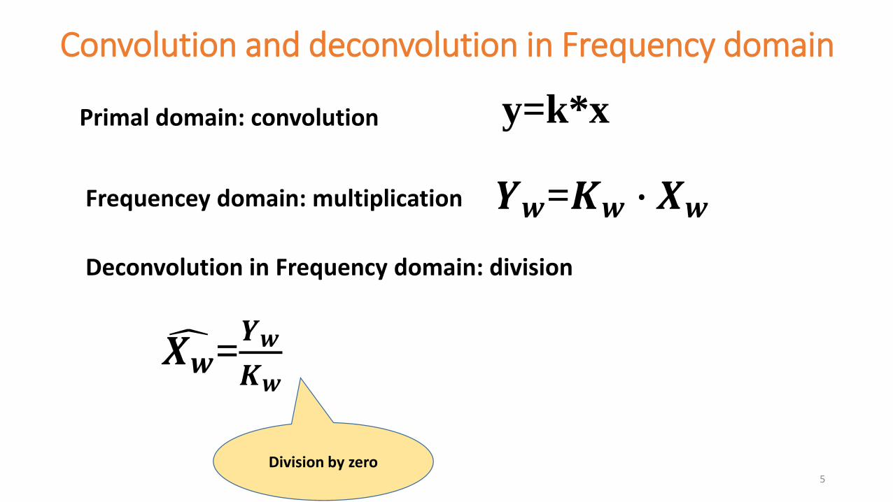
Convolution and deconvolution in Frequency domain

yxk = y=k*x

𝒀𝒘=𝑲𝒘 ∙ 𝑿𝒘

Primal domain: convolution

Frequencey domain: multiplication

Deconvolution in Frequency domain: division

𝑿𝒘=𝒀𝒘

𝑲𝒘

Division by zero

6

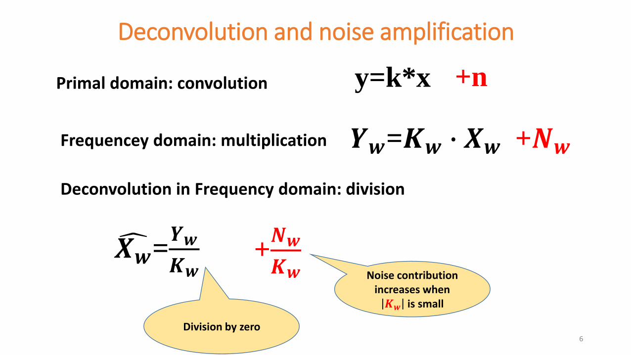
Deconvolution and noise amplification

yxk = y=k*x

𝒀𝒘=𝑲𝒘 ∙ 𝑿𝒘

Primal domain: convolution

Frequencey domain: multiplication

Deconvolution in Frequency domain: division

𝑿𝒘=𝒀𝒘

𝑲𝒘

Division by zero

+n

+𝑵𝒘

+𝑵𝒘

𝑲𝒘 Noise contribution increases when 𝑲𝒘 is small

Computational photography approaches to blurring problems

• Motion blur• Flutter shutter

• Motion invariant photography

• Defocus blur• Coded aperture

• Lattice focal

• Flexible depth of field

• Wavefront coding

Flutter Shutter

Engineer motion PSF (coding exposure time) so it becomes invertible!

[Raskar et al. 2006]

[Raskar et al. 2006]

Traditional Camera

Shutter is OPEN

[Raskar et al. 2006]

Flutter Shutter

[Raskar et al. 2006]

Shutter is OPEN and

CLOSED

[Raskar et al. 2006]

Lab Setup[Raskar et al. 2006]

Blurring

=

Convolution

Traditional Camera: Box Filter

sinc Function

[Raskar et al. 2006]

Fourier magnitudes

spatial convolution

Flutter Shutter: Coded Filter

Preserves High Frequencies!!!

[Raskar et al. 2006]

spatial convolution

Fourier magnitudes

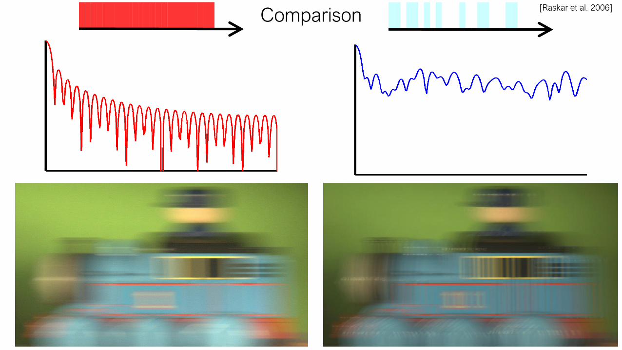
Comparison[Raskar et al. 2006]

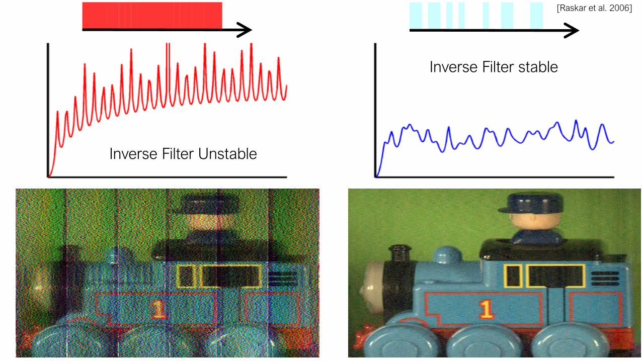
Inverse Filter Unstable

Inverse Filter stable

[Raskar et al. 2006]

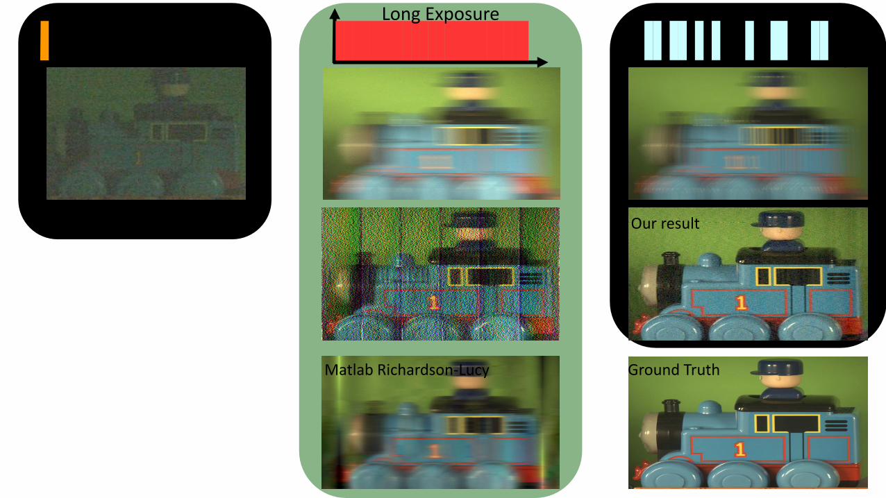
Short Exposure Long Exposure Coded Exposure

Ground TruthMatlab Richardson-Lucy

Our result

Are all codes “good”?

Alternate

All ones

Random

Our Code

[Raskar et al. 2006]

License Plate Retrieval

[Raskar et al. 2006]

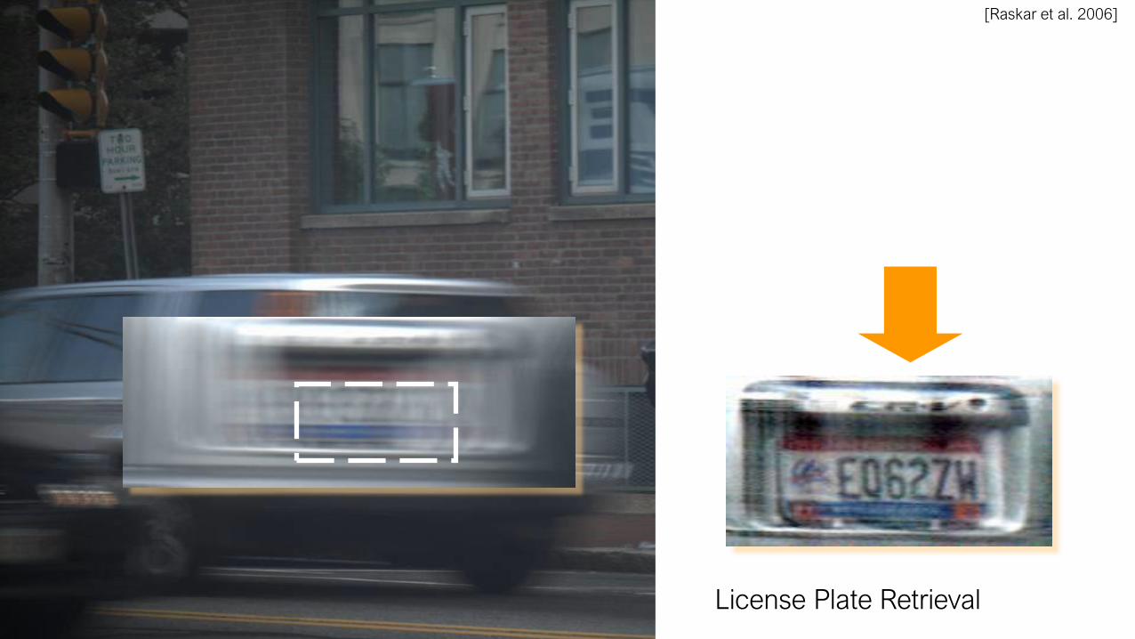
License Plate Retrieval

[Raskar et al. 2006]

Computational photography approaches to blurring problems

• Motion blur• Flutter shutter

• Motion invariant photography

• Defocus blur• Coded aperture

• Lattice focal

• Flexible depth of field

• Wavefront coding

23

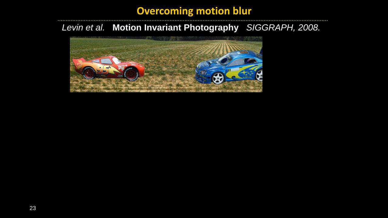
Overcoming motion blur

Levin et al. Motion Invariant Photography SIGGRAPH, 2008.

24

Overcoming motion blur

Levin et al. Motion Invariant Photography SIGGRAPH, 2008.

Removing motion blur is hard:

• Need to know exact motion velocity (blur kernel)

• Need to segment image

Deblurring red car

25

Overcoming motion blur

Levin et al. Motion Invariant Photography SIGGRAPH, 2008.

26

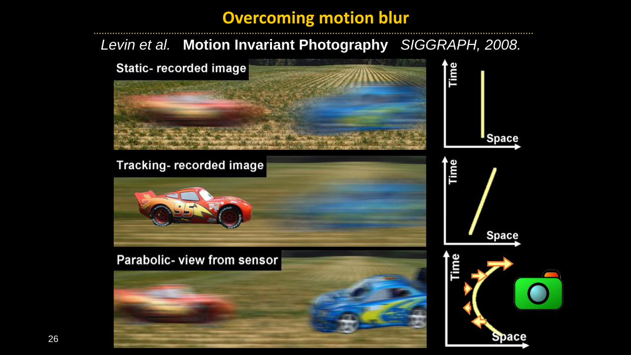
Overcoming motion blur

Levin et al. Motion Invariant Photography SIGGRAPH, 2008.

27

Overcoming motion blur

Levin et al. Motion Invariant Photography SIGGRAPH, 2008.

Motion invariant blur

28

Overcoming motion blurMotion Invariant PhotographyLevin et al. Motion Invariant Photography SIGGRAPH, 2008.

Motion invariant deblurring

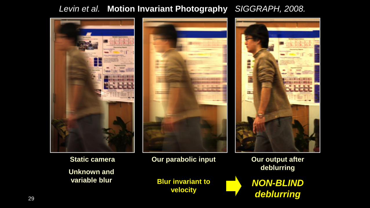
29

Static camera

Unknown and

variable blur

Our parabolic input

Blur invariant to

velocity

Our output after

deblurring

NON-BLIND

deblurring

Levin et al. Motion Invariant Photography SIGGRAPH, 2008.

The space time volume

xyt- space-time volume

xt-slice

x

y

x

t

t

The space time volume

xt-slice

x

Static objects- vertical lines

Moving objects slanted lines, slope ~ motion velocity

t

Camera integration

t

x

captured image (1D)

Static objects- sharp

Moving objects- blurred

Pixel integration curves

Shearing

x

Static object coordinates

x’

Moving object coordinates

t t

Coordinate

change

Shearing: ),( tstx −→),( tx

Shearing

t

x x

Shearing: ),( tstx −→),( tx

Static object coordinates Moving object coordinates

tDisplacement:

Can we find a shear invariant integration curve?

Solution: parabolic curve!

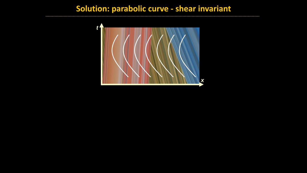
Solution: parabolic curve - shear invariant

x

t

x

Solution: parabolic curve - shear invariant

t

x

Solution: parabolic curve - shear invariant

t

x

Solution: parabolic curve - shear invariant

t

x

Solution: parabolic curve - shear invariant

t

x

Solution: parabolic curve - shear invariant

t

x

Solution: parabolic curve - shear invariant

x

Static object coordinates Moving object coordinates

Shearing: ),( tstx −→),( tx

Sheared parabola Shifted parabola

t t

x

Solution: parabolic curve - shear invariant

x

Static object coordinates Moving object coordinates

Shearing: ),( tstx −→),( tx

Sheared parabola Shifted parabola

2)( ttf = stttf s −= 2)(

( ) 4/2/ 22sst −−=

b c

t t

Solution: parabolic curve - shear invariant

For any velocity (slope),

• there is one time instant where curve is tangent

• corresponds to moment when object is tracked.

• The parabola has a linear derivative

=> spends equal time tracking each velocity.

x

t

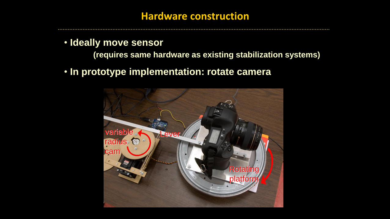
Hardware construction

• Ideally move sensor

(requires same hardware as existing stabilization systems)

• In prototype implementation: rotate camera

variable

radius

cam

Rotating

platform

Lever

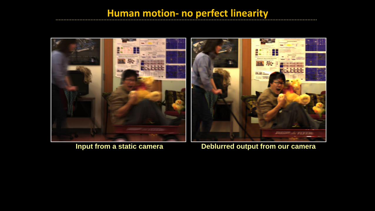
Input from a static camera Deblurred output from our camera

Human motion- no perfect linearity

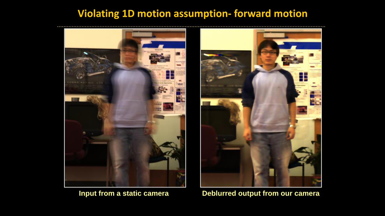
Violating 1D motion assumption- forward motion

Input from a static camera Deblurred output from our camera

Violating 1D motion assumption- stand-up motion

Input from a static camera Deblurred output from our camera

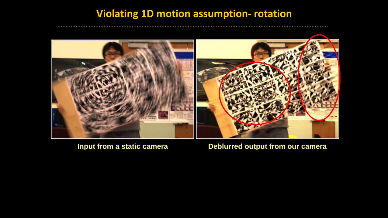
Violating 1D motion assumption- rotation

Input from a static camera Deblurred output from our camera

Limitations & approximations

Limitations:

• 1-D velocity

• Pre-defined velocities range

Approximations:

• PSFs differs in boundaries for different velocities

• Deblurred objects captured at different times

PSF

x

51

Uniqueness & optimality

• Uniqueness – Parabola is the only shear invariant curve

• Optimality – Most stable inversion of PSF: 𝑝𝑠𝑓(𝑤)−1 is the highest you can get,

provably.

𝑦 = 𝑝𝑠𝑓 ∗ 𝑥

ො𝑦 = 𝑝𝑠𝑓 ∙ ෝ𝑥

𝑝𝑠𝑓−1 ∙ ො𝑦 = ෝ𝑥

ℱ

∎−1

52

Computational photography approaches to blurring problems

• Motion blur• Flutter shutter

• Motion invariant photography

• Defocus blur• Coded aperture

• Lattice focal

• Flexible depth of field

• Wavefront coding

Image and Depth from a Conventional Camera with a Coded Aperture

Anat Levin, Rob Fergus, Frédo Durand, William Freeman

54

Coded aperture - Introduction

Problem:

Objects that are not in focus seem blurry.

Goal:Single input image:

Output #1: Depth map

Output #2: All-focused image

55

LensCamera sensor

Point spread function

Image of a point light

source

Focal plane

Lens’ aperture

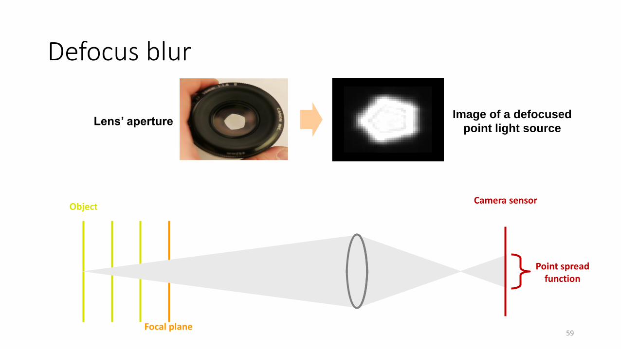
Defocus blur

56

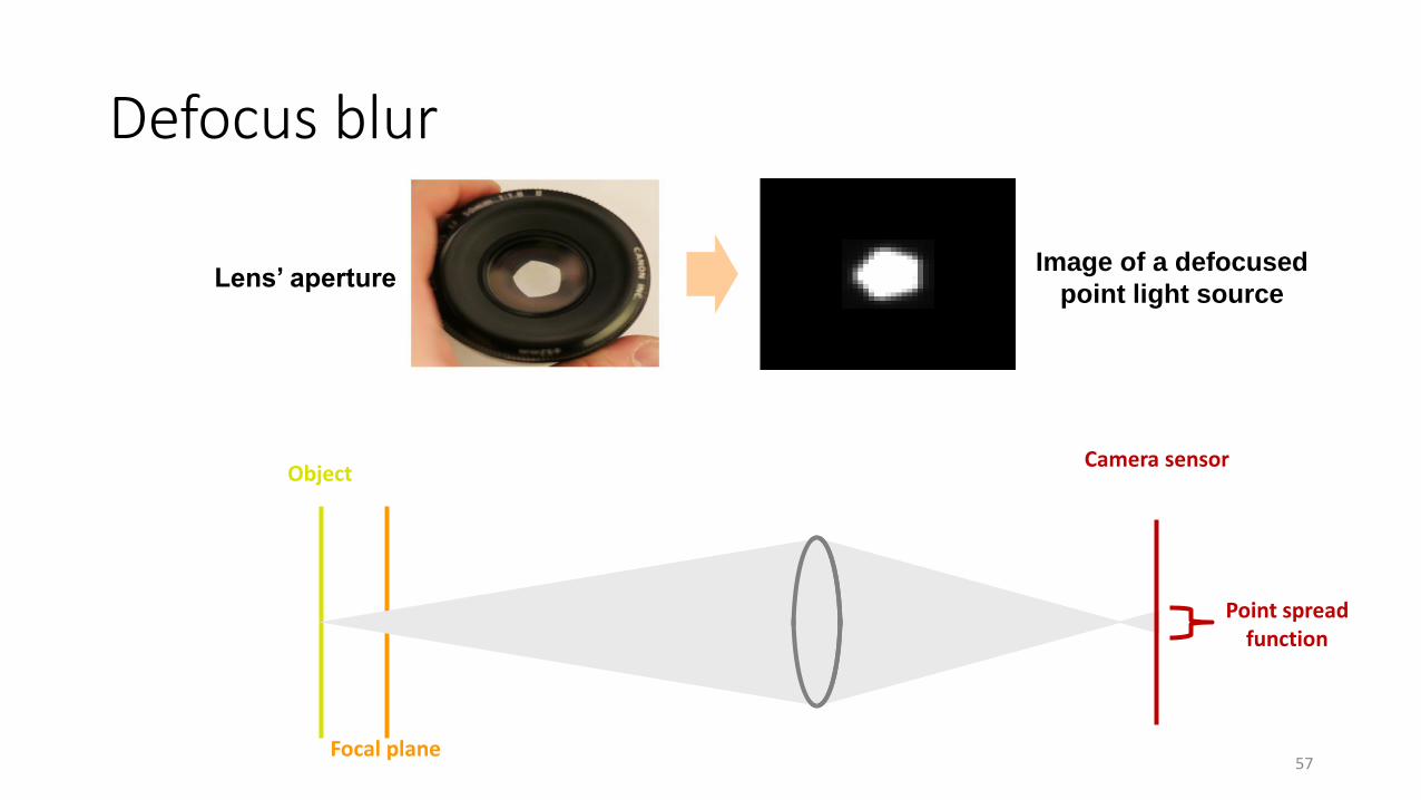
LensObjectCamera sensor

Point spread function

Focal plane

Defocus blur

Image of a defocused

point light sourceLens’ aperture

57

LensCamera sensor

Point spread function

Object

Focal plane

Defocus blur

Lens’ aperture Image of a defocused

point light source

58

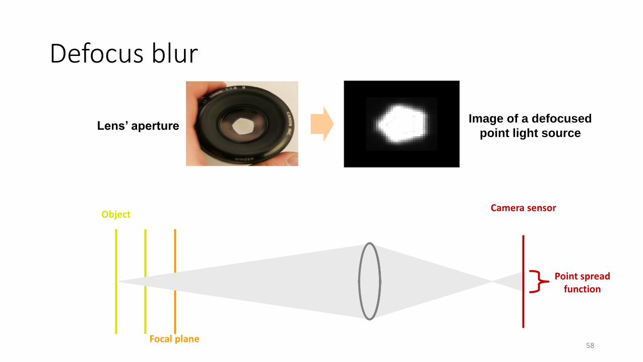
LensCamera sensor

Point spread function

Object

Focal plane

Defocus blur

Lens’ aperture Image of a defocused

point light source

59

LensCamera sensor

Point spread function

Object

Focal plane

Defocus blur

Lens’ aperture Image of a defocused

point light source

Blur ↔ Depth ↔ PSF (Filter) Scale

60

1-D Frequency analysis

Time

FrequencyFrequency

Time

Larger filter scale

Loss of high frequencies

Reconstruction is difficult 61

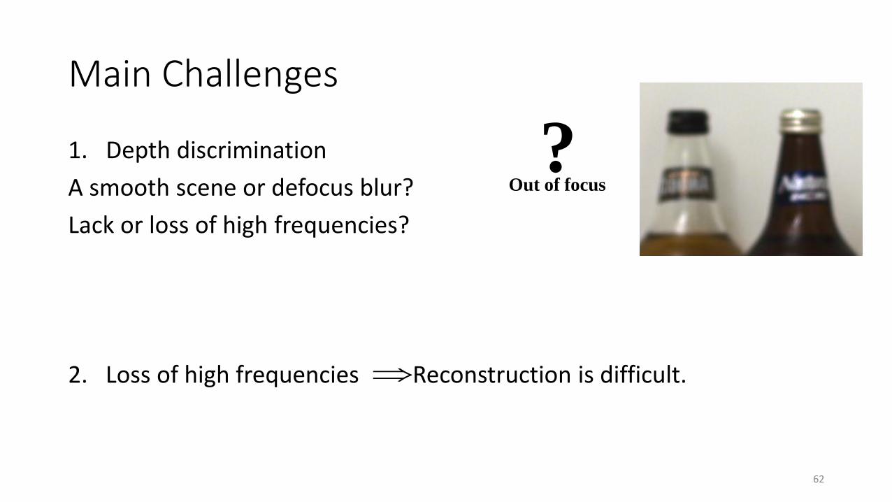
Main Challenges

1. Depth discrimination

A smooth scene or defocus blur?

Lack or loss of high frequencies?

2. Loss of high frequencies Reconstruction is difficult.

Out of focus?

62

Coded aperture

• Mask within the aperture of the lens

• Defocus patterns differ from natural images => Easier depth discrimination

• Defocus kernel preserves more high frequencies (not a LPF)

63

64

65

Lens with coded

aperture

Focal plane

Camera sensor

Point spread function

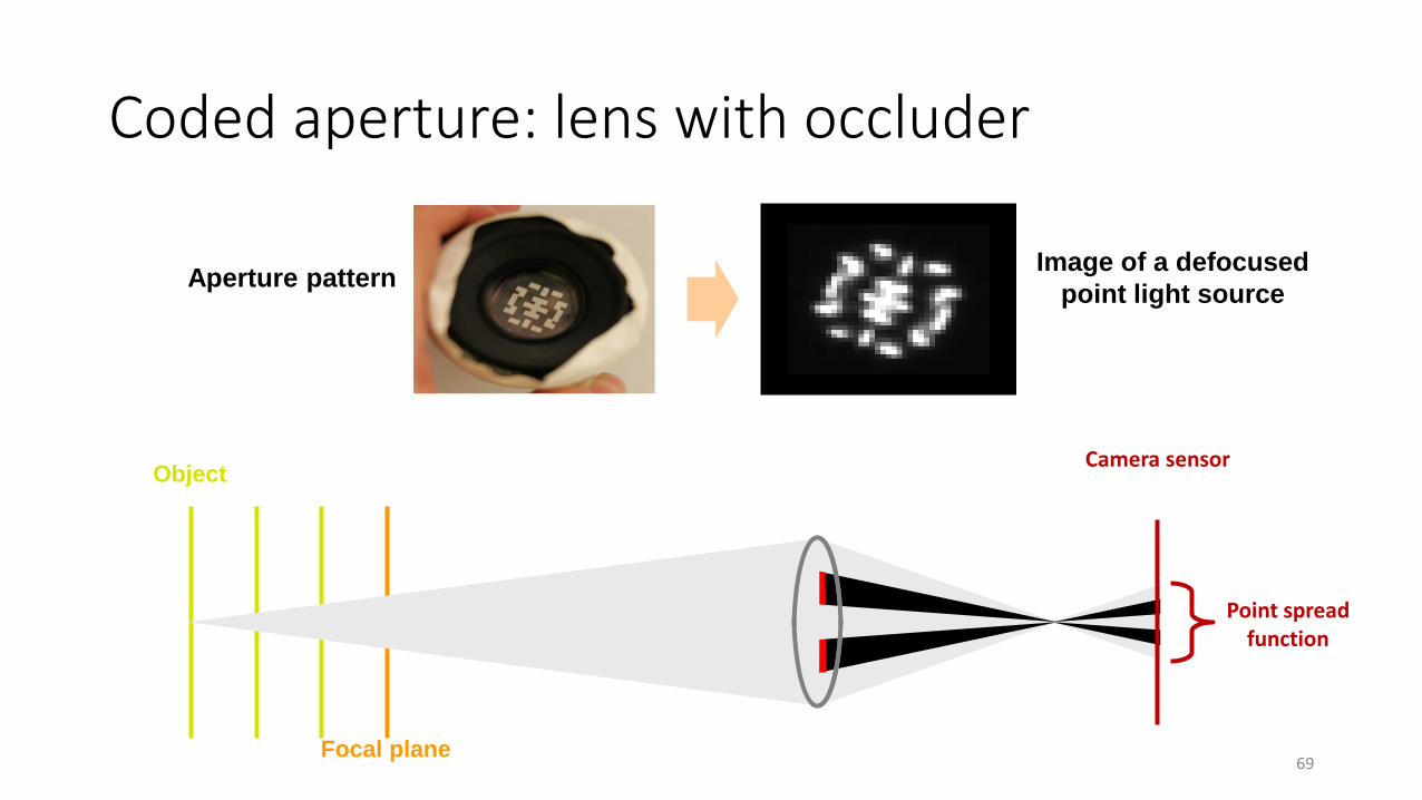
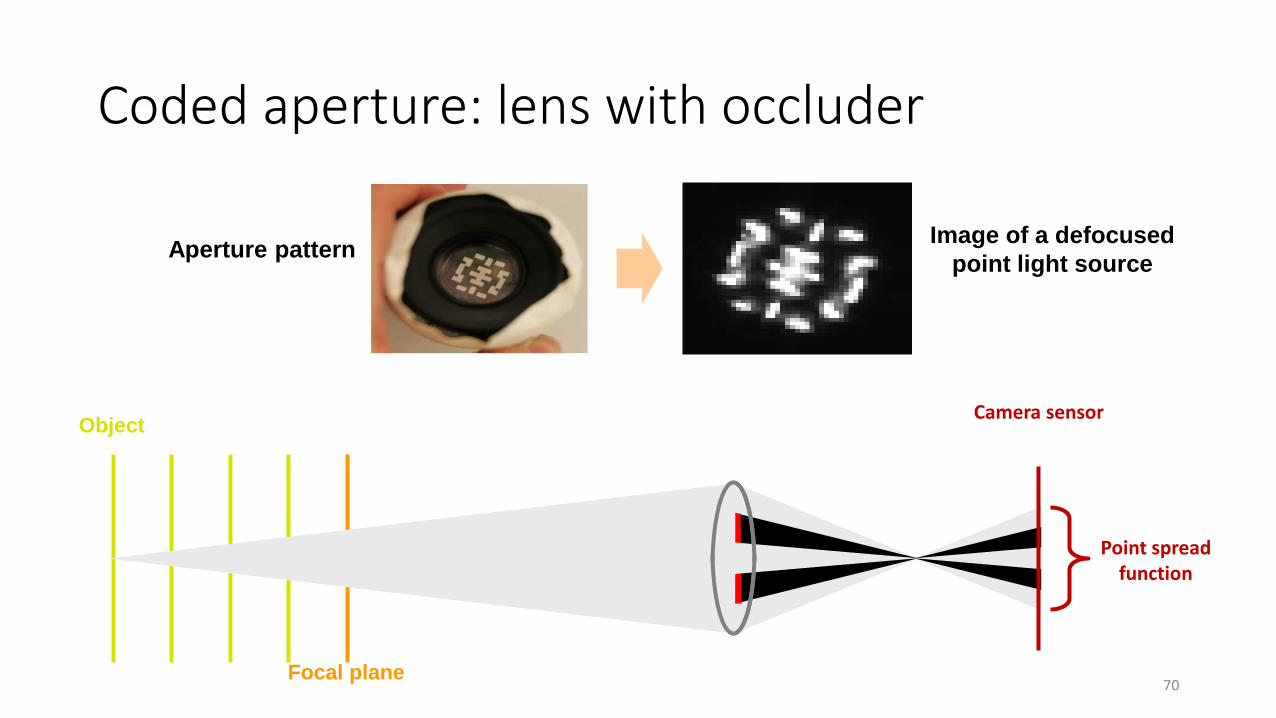
Coded aperture: lens with occluder

Image of a point light

sourceAperture pattern

66

Lens with coded

aperture

Object

Focal plane

Camera sensor

Point spread function

Coded aperture: lens with occluder

Image of a defocused

point light sourceAperture pattern

67

Lens with coded

aperture

Object

Focal plane

Camera sensor

Point spread function

Coded aperture: lens with occluder

Image of a defocused

point light sourceAperture pattern

68

Lens with coded

aperture

Object

Focal plane

Camera sensor

Point spread function

Coded aperture: lens with occluder

Image of a defocused

point light sourceAperture pattern

69

Lens with coded

aperture

Object

Focal plane

Camera sensor

Point spread function

Coded aperture: lens with occluder

Image of a defocused

point light sourceAperture pattern

70

Image of a point light source

Captured ImageCaptured Image

Conventional

Aperture

Defocused images≠ natural images!

Coded

Aperture

71

Conventional Coded

Correct scale

Smaller scale

Larger scale

Scale estimation - comparison

72

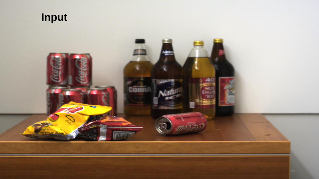
Input

83

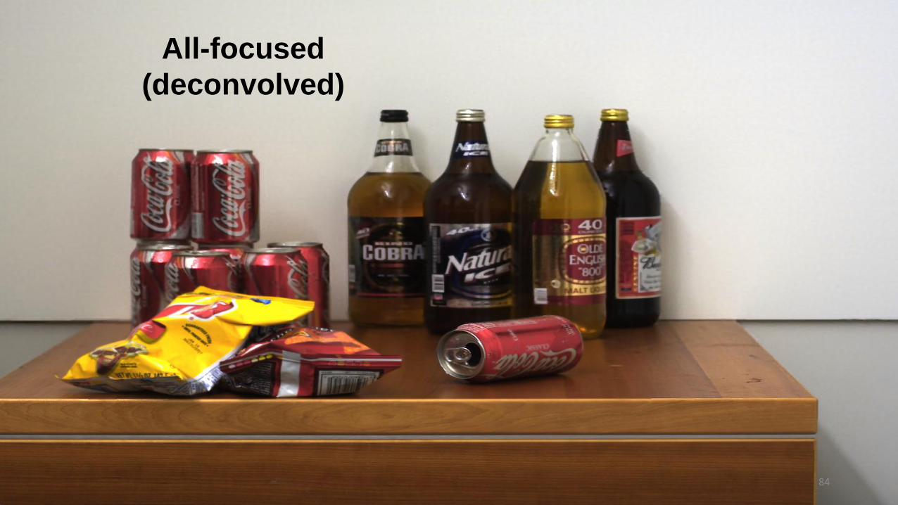
All-focused

(deconvolved)

84

Input

85

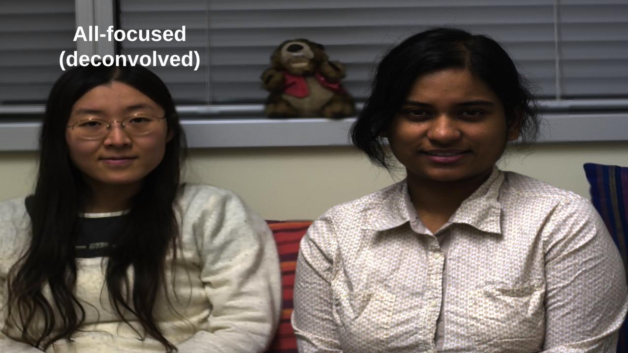
All-focused

(deconvolved)

86

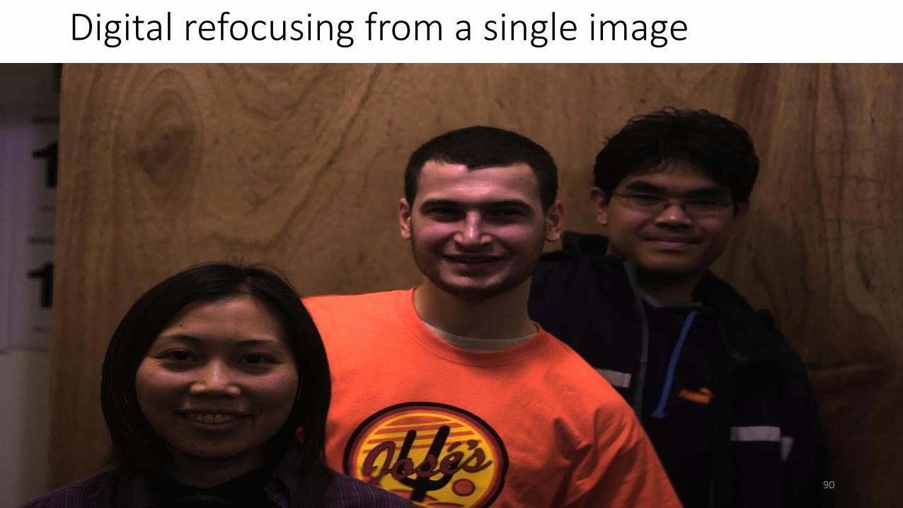
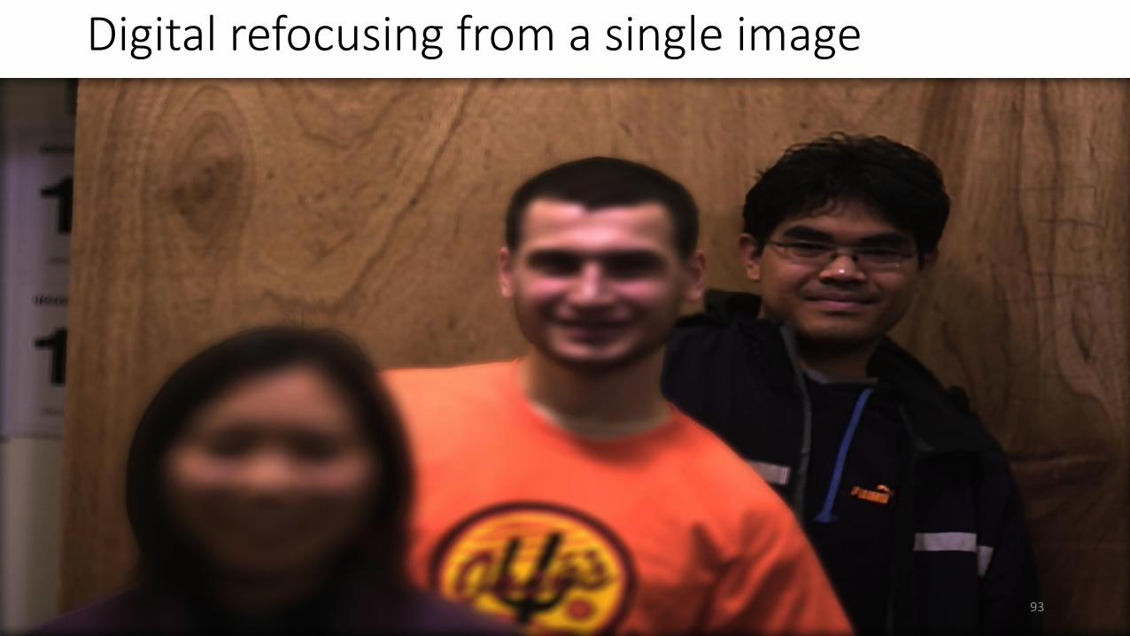
Digital refocusing from a single image

90

Digital refocusing from a single image

91

Digital refocusing from a single image

92

Digital refocusing from a single image

93

Digital refocusing from a single image

94

Digital refocusing from a single image

95

Digital refocusing from a single image

96

Disadvantages of coded aperture

[Levin et al. 2009]

Blocks light

OTF still have zeros and not so easy to invert

Another solution: Lattice focal lens

Does not block light

OTF as high as possible

Lattice Focal Lens

[Levin et al. 2009]

superimpose array of lenses with

different focal lengths!

time

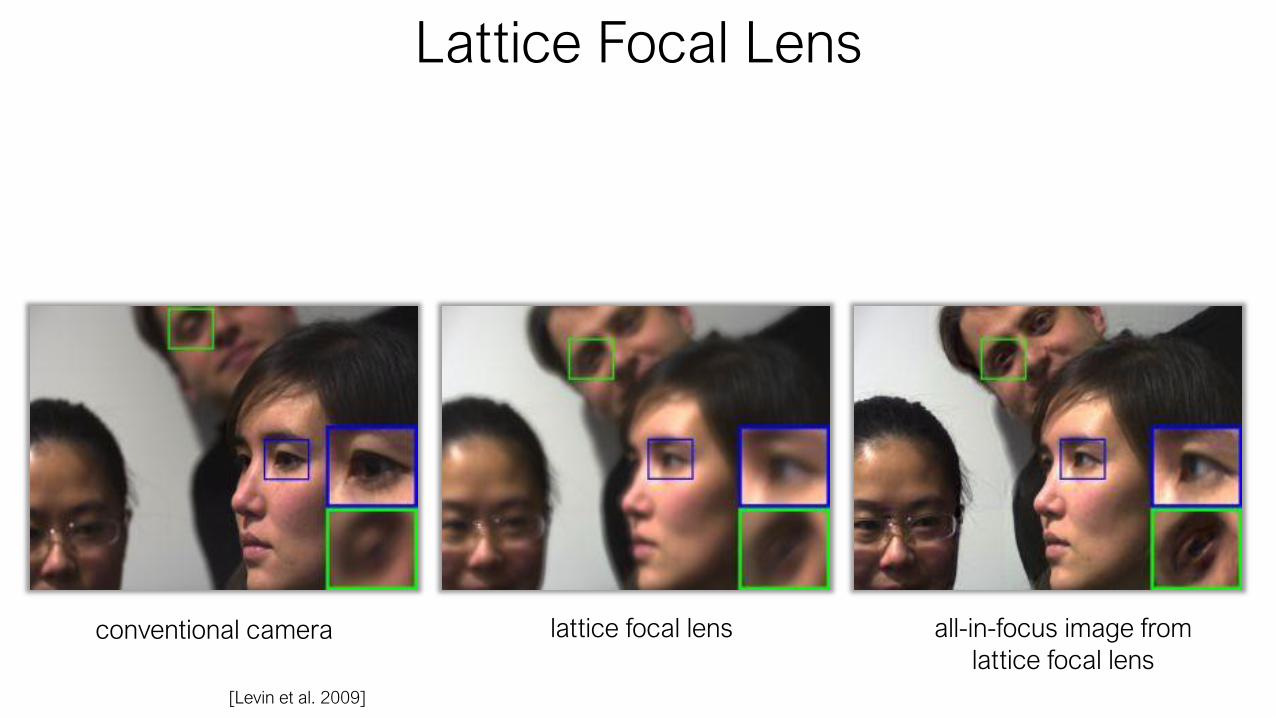
Lattice Focal Lens

[Levin et al. 2009]

conventional camera lattice focal lens all-in-focus image from

lattice focal lens

Computational photography approaches to blurring problems

• Motion blur• Flutter shutter

• Motion invariant photography

• Defocus blur• Coded aperture

• Lattice focal

• Flexible depth of field

• Wavefront coding

Flexible Depth of Field PhotographyHajime Nagahara, Sujit Kuthirummal,Changyin Zhou, and Shree K. Nayar

101

Flexible Depth of Field Photography

Problem:

Objects that are not in focus seem blurry.

Goal:

• Compute extended DOF (all-focus image) from a single image.

• Change imaging scheme to achieve depth-invariant blur so computational deblurring is easier

102

Main Challenge

• Trade-off between DOF and SNR

• A lens with a greater f-number projects darker images

103

LensCamera sensor

Point spread function

Focal plane

Main Challenge

• Trade-off between DOF and SNR

• A lens with a greater f-number projects darker images

LensCamera sensor

Point spread function

Object

Focal plane104

105

Flexible Depth of Field

106

107

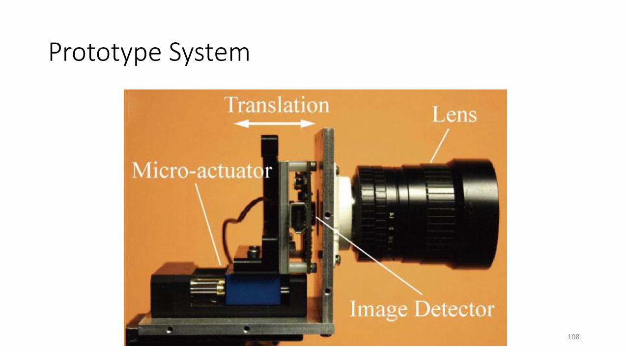
Prototype System

108

Extended Depth of Field

Captured Image(f/1.4, T=0.36sec) Computed EDOF Image

Image from Normal Camera (f/1.4, T=0.36sec, Near Focus)

Image from Normal Camera (f/8, T=0.36sec, Near Focus) with Scaling109

Uniformkernel

Extended Depth of Field: Low Light Imaging

Captured Image(f/1.4, T=0.72sec)

Computed EDOF Image Image from Normal Camera(f/1.4, T=0.72sec, Near Focus)

Image from Normal Camera(f/8, T=0.72sec, Near Focus) with Scaling

110

Wavefront Coding

• how to obtain a depth invariant PSF without mechanically moving parts

→ change the lens!

[Dowski and Cathey 1995]

cubic phase plate

Lattice Focal Lens

[Levin et al. 2009]

superimpose array of lenses with

different focal lengths!

time

Wavefront Coding v.s. lattice focal

time

f1

f2

f3

f4

f1 f2

f3 f4

Cubic phase plate Lattice focal phase plate

A focal area

d1 d2 d3 d4

Extended DOF Solutions

• Coded aperture

• Wavefront coding

• Focal Sweep

• Lattice-Focal

121

-> Highest possible OTF

Depth invariant

Need to estimate depth as part of inversion