This discussion paper is/has been under review for the journal Atmospheric Chemistryand Physics (ACP). Please refer to the corresponding final paper in ACP if available.
The Amazon Tall Tower Observatory(ATTO) in the remote Amazon Basin:overview of first results from ecosystemecology, meteorology, trace gas, andaerosol measurementsM. O. Andreae1,2, O. C. Acevedo3, A. Araùjo4, P. Artaxo5, C. G. G. Barbosa6,H. M. J. Barbosa5, J. Brito5, S. Carbone5, X. Chi1, B. B. L. Cintra7, N. F. da Silva7,N. L. Dias6, C. Q. Dias-Júnior8,11, F. Ditas1, R. Ditz1, A. F. L. Godoi6,R. H. M. Godoi6, M. Heimann9, T. Hoffmann10, J. Kesselmeier1, T. Könemann1,M. L. Krüger1, J. V. Lavric9, A. O. Manzi11, D. Moran-Zuloaga1, A. C. Nölscher1,D. Santos Nogueira12,**, M. T. F. Piedade7, C. Pöhlker1, U. Pöschl1, L. V. Rizzo5,C.-U. Ro13, N. Ruckteschler1, L. D. A. Sá14, M. D. O. Sá15, C. B. Sales11,16,R. M. N. D. Santos17, J. Saturno1, J. Schöngart1,7, M. Sörgel1, C. M. deSouza11,18, R. A. F. de Souza17, H. Su1, N. Targhetta7, J. Tóta17,19, I. Trebs1,*,S. Trumbore9, A. van Eijck10, D. Walter1, Z. Wang1, B. Weber1, J. Williams1,J. Winderlich1,9, F. Wittmann1, S. Wolff1,11, and A. M. Yáñez-Serrano1,11
1Biogeochemistry, Multiphase Chemistry, and Air Chemistry Departments, Max PlanckInstitute for Chemistry, P.O. Box 3060, 55020, Mainz, Germany2Scripps Institution of Oceanography, University of California San Diego, La Jolla, CA 92037,USA3Universidade Federal Santa Maria, Dept. Fisica, 97119900 Santa Maria, RS, Brazil4Empresa Brasileira de Pesquisa Agropecuária (EMBRAPA), Trav. Dr. Enéas Pinheiro,Belém-PA, CEP 66095-100, Brazil5Instituto de Física, Universidade de São Paulo (USP), Rua do Matão, Travessa R, 187, CEP05508-900, São Paulo, SP, Brazil6Department of Environmental Engineering, Federal University of Paraná UFPR, Curitiba, PR,Brazil7Instituto Nacional de Pesquisas da Amazônia (INPA), MAUA group, Av. André Araújo 2936,Manaus-AM, CEP 69067-375, Brazil8Instituto Nacional de Educação, Ciência e Tecnologia do Pará (IFPA/Bragança), Pará, Brazil9Max Planck Institute for Biogeochemistry, Hans-Knöll-Straße 10, 07745 Jena, Germany10Department of Chemistry, Johannes Gutenberg University, Mainz, Germany11Instituto Nacional de Pesquisas da Amazônia (INPA), Clima e Ambiente (CLIAMB), Av.André Araújo 2936, Manaus-AM, CEP 69083-000, Brazil12Centro Gestor e Operacional do Sistema de Proteção da Amazônia (CENSIPAM), Belém,Pará, Brazil13Department of Chemistry, Inha University, Incheon 402-751, Korea14Centro Regional da Amazônia, Instituto Nacional de Pesquisas Espaciais (INPE), Belém,Pará, Brazil15Instituto Nacional de Pesquisas da Amazônia (INPA), LBA, Av. André Araújo 2936,Manaus-AM, CEP 69067-375, Brazil16Centro de Estudos Superiores de Parintins (CESP/UEA), Parintins, Amazonas, Brazil17Universidade do Estado do Amazonas (UEA), Manaus, Amazonas, Brazil18Universidade Federal do Amazonas (UFAM/ICSEZ-Parintins), Parintins, Amazonas, Brazil19Universidade Federal do Oeste do Pará – UFOPA, Santarém, Pará, Brazil*now at: Luxembourg Institute of Science and Technology, Environmental Research andInnovation (ERIN) Department, 4422 Belvaux, Luxembourg
The Amazon Basin plays key roles in the carbon and water cycles, climate change,atmospheric chemistry, and biodiversity. It already has been changed significantly byhuman activities, and more pervasive change is expected to occur in the next decades.It is therefore essential to establish long-term measurement sites that provide a base-5
line record of present-day climatic, biogeochemical, and atmospheric conditions andthat will be operated over coming decades to monitor change in the Amazon region ashuman perturbations increase in the future.
The Amazon Tall Tower Observatory (ATTO) has been set up in a pristine rain forestregion in the central Amazon Basin, about 150 km northeast of the city of Manaus. An10
ecological survey including a biodiversity assessment has been conducted in the for-est region surrounding the site. Two 80 m towers have been operated at the site since2012, and a 325 m tower is nearing completion in mid-2015. Measurements of mi-crometeorological and atmospheric chemical variables were initiated in 2012, and theirrange has continued to broaden over the last few years. The meteorological and mi-15
crometeorological measurements include temperature and wind profiles, precipitation,water and energy fluxes, turbulence components, soil temperature profiles and soil heatfluxes, radiation fluxes, and visibility. A tree has been instrumented to measure stemprofiles of temperature, light intensity, and water content in cryptogamic covers. Thetrace gas measurements comprise continuous monitoring of carbon dioxide, carbon20
monoxide, methane, and ozone at 5 to 8 different heights, complemented by a vari-ety of additional species measured during intensive campaigns (e.g., VOC, NO, NO2,and OH reactivity). Aerosol optical, microphysical, and chemical measurements aremade above the canopy as well as in the canopy space. They include light scatteringand absorption, aerosol fluorescence, number and volume size distributions, chemical25
composition, cloud condensation nuclei (CCN) concentrations, and hygroscopicity. Ini-tial results from ecological, meteorological, and chemical studies at the ATTO site arepresented in this paper.
A little over thirty years ago, Eneas Salati and Peter Vose published a landmark paperentitled “Amazon Basin: A System in Equilibrium” (Salati and Vose, 1984). Since then,a paradigm shift has occurred in the minds of the public at large as well as the scien-tific community, which is reflected in the title of a recent synthesis paper by a group5
of prominent Amazon researchers, “The Amazon Basin in transition” (Davidson et al.,2012). Despite its reassuring title, Salati and Vose’s paper had already pointed at grow-ing threats to the integrity of the Amazon ecosystem, mostly resulting from continuedlarge-scale deforestation. Deforestation has indeed continued, and has only begunto abate in recent years. It goes hand in hand with road construction and urbaniza-10
tion (Fraser, 2014), affecting ecosystems and air quality in many parts of the Basin.And, whereas Salati and Vose were concerned with climate change as a regional phe-nomenon driven by deforestation and its impact on the hydrological cycle, the focusnow is on the interactions of global climate change with the functioning of the Ama-zon forest ecosystem (Keller et al., 2009). In the following sections, we will present the15
key roles the Amazon is playing in the global ecosystem, which form the rationale forsetting up a long-term measuring station for monitoring its functioning and health.
1.1 Carbon cycle
The Amazon Basin covers about one third of the South American continent and extendsover about 6.9×10⁶ km2, of which about 80 % is covered with rain forest (Goulding20
et al., 2003). It contains 90–120 PgC in living biomass, representing about 84 % of theaboveground biomass in Latin America and ca. 40 % of all tropical forests worldwide(Baccini et al., 2012; Gloor et al., 2012). Another 160 PgC are stored in the Amazon’ssoils – putting this in perspective, the Amazon holds about half as much carbon as wasin the Earth’s atmosphere before the industrial revolution (Gloor et al., 2012). Given the25
magnitude of this carbon reservoir, it is clear that tropical forests in general, and theAmazon forest in particular, have the potential to play a crucial role in climate change
because of their potential to gain or lose large amounts of carbon as a result of land useand climate change. A recent study shows a strong correlation between climate changeon the tropical continents and the rate at which CO2 increases in the atmosphere, andindicates that the strength of this feedback has doubled since the 1970s (Wang et al.,2014). The interaction between physical climate and the biosphere represents one of5
the largest uncertainties in the assessment of the response of the climate system tohuman emissions of greenhouse gases.
Depending on the path land use change takes and the interactions between the for-est biota and the changing climate, the Amazon can act as a net source or sink ofatmospheric CO2. The most recent global carbon budget estimates indicate that in the10
decade of 2004–2013 land use change worldwide resulted in a net carbon release of0.9±0.5 Pga−1, or about 9 % of all anthropogenic carbon emissions (Le Quéré et al.,2014). This represents a significant decrease since the 1960s, when land-use carbonemissions of 1.5±0.5 Pga−1 accounted for 38 % of anthropogenic CO2. Part of this de-crease in the relative contribution from land use change is of course due to the increase15
in fossil fuel emissions, but there has been a significant decrease in deforestation inrecent years, particularly in the Brazilian Amazon (Nepstad et al., 2014).
The “net” land use emissions, as presented above, are always the sum of “gross”release and uptake fluxes, where deforestation represents the dominant gross source,and afforestation, regrowth, and uptake by intact vegetation, the main gross sinks. Us-20
ing an approach based on forest inventories and land use budgeting, Pan et al. (2011)estimated that tropical land use change represented a net carbon source of 1.3±0.7 Pga−1 in the 1990s and early 2000s, consisting of a gross tropical deforestationcarbon emission of 2.9±0.5 Pga−1 partially compensated for by a carbon sink in trop-ical forest regrowth of 1.6±0.5 Pga−1. A comprehensive analysis of the role of land25
vegetation in the global carbon cycle concluded that carbon sources and sinks in thetropics are approximately balanced, with regrowth and CO2-driven carbon uptake com-pensating the large deforestation source (Schimel et al., 2015). For the South Americancontinent, a detailed budgeting study also concluded that carbon uptake by the bio-
sphere at present approximately compensates the emissions from deforestation andfossil fuel burning, with a slight trend in the continent becoming a source in the mostrecent period (Gloor et al., 2012).
Attempts to verify these carbon budgets with measurements have remained incon-clusive so far. The largest spatial scale is represented by global inversion models,5
which derive fluxes from concentration measurements and global transport models. Anearly attempt deduced a large tropical sink from inverse modeling (Stephens et al.,2007), whereas a more recent analysis suggests a net tropical carbon source of1.1±0.9 Pga−1 (Steinkamp and Gruber, 2013). Gloor et al. (2012) have reviewed thenumerous attempts to deduce the South American carbon budgets from inverse mod-10
eling and came to the conclusion that they are not adequately constrained to producemeaningful results, a conclusion that they extend to the application of digital globalvegetation models for larger time and space scales.
Efforts to upscale local measurements to larger scales have also lead to inconclu-sive and often contradictory results. Flux measurements using the eddy covariance15
technique initially suggested a fairly large carbon sink (1–8 tha2 a−1) in intact Ama-zon forests (e.g., Grace et al., 1995; Carswell et al., 2002; de Araújo et al., 2002).But as more studies were conducted, this range expanded from a sink of 8 tha−2 a−1 toa source of 1.4 tha−2 a−1, and it became clear that issues related to nighttime fluxes andterrain effects make upscaling of CO2 fluxes from eddy covariance measurements dif-20
ficult to impossible (de Araujo et al., 2010, and references therein). Nevertheless, suchflux measurements are essential for understanding micrometeorological and ecologicalprocesses and for monitoring changes in the functioning of the forest ecosystem.
An alternative approach to upscaling from local to regional carbon balances is fol-lowed in the RAINFOR project, where some 140 forest plots have been monitored over25
decades for standing biomass (Phillips et al., 2009). This study suggested substantialcarbon uptake by intact forest, interrupted by biomass loss during drought years. Ithas been proposed that a large fraction of the uptake extrapolated from the RAINFORsites is compensated by rare disturbance events, such as forest blow-downs resulting
from severe thunderstorms (Chambers et al., 2013, and references therein). The latestanalysis from the RAINFOR project, now based on 321 plots and 25 years of data, indi-cates that the Amazon carbon sink in intact forest has declined by one-third during thepast decade compared to the 1990s. This appears to be driven by increased biomassmortality, possibly caused by greater climate variability and feedbacks of faster growth5
on mortality (Brienen et al., 2015). Like flux-tower measurements, biomass inventoriesalso miss the contributions of wetlands and water bodies to the carbon flux, which maymake a substantial contribution to CO2 outgassing (Richey et al., 2002; Abril et al.,2014).
An intermediate scale between global inverse modeling and plot-size flux and in-10
ventory studies is captured by aircraft soundings of CO2 through the lowest few km ofthe troposphere. This method averages regional fluxes on scales of tens to hundredsof km. Early measurements during the 1987 ABLE-2 experiment were reanalyzed byChou et al. (2002), and suggested a near-neutral carbon balance for their study regionnear Manaus. A series of flights north of Manaus during the 2001 wet-to-dry transi-15
tion season also revealed that daytime carbon uptake and nighttime release were inapproximate balance (Lloyd et al., 2007). A 10 year aircraft profiling study conductednear Santarem in the eastern Amazon concluded that the fetch region was a small netcarbon source (0.15 tha−2 a−1), mostly as a result of biomass burning, with no signif-icant net flux to or from the forest biosphere (Gatti et al., 2010). In 2010, this study20
was extended to include the southern and western parts of the Amazon Basin (Gattiet al., 2014). The results from 2010, an unusually dry year, show the Amazon forestbiosphere to be sensitive to drought, resulting in net carbon emission from the vege-tation. The following year, 2011, was wetter than average, and the Basin returned toan approximately neutral carbon balance, with a modest biospheric sink compensating25
the biomass burning source.Seen together, these studies suggest that the Amazon Basin teeters on a precarious
balance between being a source or sink of carbon to the world’s atmosphere, with its fu-ture depending on the extent and form of climate change as well as on human actions.
The region has already warmed by 0.5–0.6 ◦C, and warming is expected to continue(Malhi and Wright, 2004). Together with the increased frequency of drought episodes(Saatchi et al., 2013), the occurrence of periods of net biospheric carbon emissionswill be enhanced and the likelihood of destructive understory fires will increase (Glooret al., 2013; Balch, 2014; Zeri et al., 2014). On the other hand, the observed 20 %5
increase in Amazon River discharge may reflect an increasing water supply to the veg-etation (Gloor et al., 2013), which together with increasing atmospheric CO2 may leadto more net carbon uptake by the intact forest vegetation (Schimel et al., 2015). Whileremote sensing can provide important information on the response of the Amazon for-est to changing climate and ecological factors, the recent controversy about the effects10
of seasonal change and drought on the “greenness” of the forest illustrates how im-portant long-term ground based observations are to our understanding of the Amazonsystem (Soudani and Francois, 2014; Zeri et al., 2014).
Ultimately, the fate of the carbon stored in the Amazon Basin will depend on the inter-acting and often opposing effects of human actions, especially deforestation, global and15
regional climate change, and changing atmospheric composition (Soares-Filho et al.,2006; Poulter et al., 2010; Rammig et al., 2010; Davidson et al., 2012; Cirino et al.,2014; Nepstad et al., 2014; Schimel et al., 2015; Zhang et al., 2015). Interactions ofthe carbon cycle with the cycles of other key biospheric elements, especially nitrogenand phosphorus are also likely to play important roles (Ciais et al., 2013). This applies20
equally to two other greenhouse gases, methane (CH4) and nitrous oxide (N2O), bothof which have important sources in the Amazon wetlands or soils (Miller et al., 2007;D’Amelio et al., 2009; Beck et al., 2012).
1.2 Water and energy cycle
The Amazon River has by far the greatest discharge of all the World’s rivers – about25
20 % of the world’s freshwater discharge and five times that of the Congo, the nextlargest river in discharge. This reflects the immense amount of water that is cyclingthrough the water bodies, soils, plants, and atmosphere of the Amazon Basin. As a re-
sult, the hydrological cycle of the Amazon Basin is crucial for providing the water thatsupports life within the Basin and even beyond its borders. Most moisture enters theBasin from the Atlantic Ocean with the trade wind circulation, but recirculation of waterthrough evapotranspiration maintains a flux of precipitation that becomes increasinglymore important as airmasses move into the western part of the Basin (Spracklen et al.,5
2012). When reaching the Andes, moisture becomes deflected southward, with theresult that Amazonian evaporation even supports the rain-fed agriculture in Argentina(Gimeno et al., 2012). As a result, perturbations of the Amazonian moisture flux andthe effects of smoke aerosols from fires in Amazonia on cloud processes can affectrainfall even over the distant La Plata Basin (Camponogara et al., 2014; Zemp et al.,10
2014).Evaporation of water from the Earth’s surface also supports a huge energy flux in
the form of latent heat, which is converted to sensible heat and atmospheric buoy-ancy when the water vapor condenses to cloud droplets. This heat transfer representsone of the major forces that drive atmospheric circulation at all scales (Nobre et al.,15
2009). Changes in land cover, e.g., conversion of forest to pasture, alter the amountand type of clouds over the region (e.g., Heiblum et al., 2014) and shift the proportionof rain that flows away as runoff vs. the fraction that is transformed to water vapor byevapo-transpiration (Silva Dias et al., 2002; Davidson et al., 2012; Gloor et al., 2013;and references therein). This in turn changes local and regional circulation and rainfall20
patterns, and consequently deforestation has been predicted to reduce the potentialfor hydropower generation in Amazonia (Stickler et al., 2013). When the scale of defor-estation exceeds some 40 % of the Basin, these perturbations of the water cycle maychange the functioning of the entire Amazon climate and ecosystem (Coe et al., 2009;Nobre and Borma, 2009).25
Our ability to prognosticate the possible outcomes for the Amazon ecosystem inthe coming decades is severely curtailed by limitations in the representation of keyprocesses in climate/vegetation models, including the role of the Andes and the tele-connections between the Amazon and the Atlantic and Pacific Oceans. In addition, the
biophysical response of the vegetation to changing water supply and increasing CO2and temperature remains very poorly understood (Davidson et al., 2012). Long-termmeasurements and process studies at key locations are urgently needed to improveour understanding of these interactions.
1.3 Biodiversity5
The Amazon Basin contains the most species-rich terrestrial and freshwater ecosys-tems in the world (Hoorn et al., 2010; Wittmann et al., 2013). It houses at least 40 000plant species, over 400 mammal, about 1300 bird, and countless numbers of inverte-brate and microbe species (da Silva et al., 2005), accounting for about 10–20 % of allthe world’s species diversity. Of these, the great majority has not yet been described10
scientifically, and possibly never will be. The variety of species in the Amazon Basin isdirectly related to the variety of habitats, and consequently is threatened by any form ofexploitation that is accompanied by habitat destruction, in particular land clearing anddeforestation. The genetic information stored in these ecosystems and their biodiver-sity is beyond measure and may be of enormous economic significance. This diversity15
is now under great threat, mostly as a result of habitat loss due to deforestation andother land use changes (Vieira et al., 2008).
Much of the Amazon’s aboveground biomass is in its trees, and a single hectareof the forest can be home to over 100 different tree species. Scientists still do notknow how many tree species occur in the Amazon, and the current estimate of about20
16 000 tree species is the result of an extrapolation from the existing scattered censusdata. Surprisingly, a relatively small number (227 species, or 1.4 %) account for halfof all individual trees (ter Steege et al., 2013), which therefore account for a largefraction of the Amazon’s ecosystem services. This fact may greatly facilitate research inAmazonian biogeochemistry, for example studies on the trace gas exchange between25
The tropical atmosphere has been referred to as the “washing machine of the atmo-sphere” by P. Crutzen (personal communication, 2013). Both human activities and thebiosphere release huge amounts of substances such as nitrogen oxides (NOx), carbonmonoxide (CO), and volatile organic compounds (VOC) into the atmosphere, which5
must be constantly removed again to prevent accumulation to toxic levels. Most suchgases are poorly soluble in water, and are thus not effectively washed out by rain. Theself-purification of the atmosphere therefore requires chemical reactions by which thetrace substances are brought into water-soluble form. These reaction chains normallybegin with an initial oxidation step in which the trace gas is attacked by a highly reactive10
molecule, such as ozone (O3) or the hydroxyl radical (OH). Production of these atmo-spheric detergents requires UV radiation and water vapor, both of which are presentin generous quantities in the tropics. It comes thus as no surprise that the tropics arethe region in which many atmospheric trace gases, including CO and CH4 are largelyeliminated (Crutzen, 1987). Recent discoveries indicate that the atmospheric oxidant15
cycles in the boundary layer are much more active than had been previously assumed,but the mechanisms of these reactions are still a matter of active research (Lelieveldet al., 2008; Martinez et al., 2010; Taraborrelli et al., 2012; Nölscher et al., 2014).
The functioning of this self-cleansing mechanism is challenged by human activitiesthat change the emissions from the biosphere and add pollutants from biomass burn-20
ing and industrial activities. This may convert the “washing machine” into a reactor pro-ducing photochemical smog with high concentrations of ozone and other atmosphericpollutants, and large quantities of fine aerosols – which in turn influence the formationof clouds and precipitation and thus modify the water cycle (Andreae, 2001; Pöschlet al., 2010). Increased ozone concentrations over Amazonia, resulting from biomass25
burning emissions, have also been implicated in plant damage, which may substantiallydecrease the carbon uptake by the Amazon forest (Pacifico et al., 2015).
The concentrations and types of aerosol particles over the Amazon Basin exhibithuge variations in time and space. In the absence of pollution from regional or dis-tant sources, and especially in the rainy season, the Amazon has among the lowestaerosol concentrations of any continental region (Roberts et al., 2001; Andreae, 2009;Martin et al., 2010b; Pöschl et al., 2010; Andreae et al., 2012; Artaxo et al., 2013; Rizzo5
et al., 2013). Biogenic aerosols, either emitted directly by the biota or produced photo-chemically from biogenic organic vapors, make up most of this “clean-period” aerosol(Martin et al., 2010a). At the other extreme, during the biomass burning season in thesouthern Amazon, aerosol concentrations over large regions are as high as in the mostpolluted urban areas worldwide (Artaxo et al., 2002; Eck et al., 2003; Andreae et al.,10
2004). These changes in the atmospheric aerosol burdens have strong impacts on theradiation budget, cloud physics, precipitation, and plant photosynthesis (Schafer et al.,2002; Williams et al., 2002; Andreae et al., 2004; Lin et al., 2006; Oliveira et al., 2007;Freud et al., 2008; Bevan et al., 2009; Martins et al., 2009; Sena et al., 2013; Cirinoet al., 2014). Episodic inputs of Saharan dust, biomass smoke from Africa, and marine15
aerosols transported over long distances with the trade winds further complicate thepicture (Formenti et al., 2001; Ansmann et al., 2009; Ben-Ami et al., 2010; Baars et al.,2011). This complexity of aerosol sources is one important reason why the mecha-nisms that lead to the production of biogenic aerosols in Amazonia are still enigmatic(Pöhlker et al., 2012; Chen et al., 2015).20
1.5 The Amazon Tall Tower Observatory (ATTO)
The foregoing sections have thrown some highlights on the key role of the AmazonBasin in the Earth System and the important ecosystem services it provides. It is ev-ident that we need a better understanding of the interactions between biosphere andatmosphere in this important region to avoid irreversible damage to this complex sys-25
tem. While considerable knowledge has been gained from campaign-style studies, it isclear that the full picture will not emerge from these “snapshots,” but that continuous,long-term studies are required at key locations (Hari et al., 2009; Zeri et al., 2014).
This is true especially in view of the fact that the Amazon and its global environmentare rapidly changing, and that continuing observations are essential to keep track ofthese changes. It is particularly urgent to obtain baseline data now, to document thepresent atmospheric and ecological conditions before upcoming changes, especially inthe eastern part of the Basin, will forever change the face of Amazonia.5
For this purpose, the Amazon Tall Tower Observatory (ATTO) has been establishedin the central Amazon Basin by a Brazilian-German partnership. The site has been setup initially with two measurement towers of intermediate height (80 m), and the con-struction of a 325 m tall tower to perform chemical and meteorological measurementsrepresenting large footprints is currently nearing completion. The tower will serve as10
a basis for continuous monitoring of long-lived biogeochemically important trace gasessuch as CO2, CH4, CO, N2O, and a multitude of reactive gases, including NOx, O3, andVOC, as well as a broad range of aerosol characteristics. The chemical measurementsare complemented by a full suite of micrometeorological measurements. Furthermore,the observing system will also include a component directed at the underlying vegeta-15
tion canopy, such as phenological observations from the tower by automated cameras,potentially a canopy lidar, as well as an array of in-situ sensors of critical physical andbiological variables in the ecosystems near the tower and the ground.
The continuous long-term data collected at ATTO will also serve to evaluate airborneand satellite observations. Expected to operate for an indeterminate length of time, this20
unique observatory in South America will provide long-term observations of the tropicalAmazonian ecosystem affected by climate change.
Specific objectives are:
1. To understand the carbon budget of the Amazonian rain forest under changingclimate conditions and anthropogenic influences.25
2. To continuously observe anthropogenic and biogenic greenhouse gases in thelower troposphere, within and outside the planetary boundary layer, in order to
help constrain inverse methods for deriving continental source and sink strengthsand their changes over time.
3. To continuously measure trace gases and aerosols for improvement of our under-standing of atmospheric chemistry and physics in the Amazon and further allowa continuous assessment of the effects of land use change on the atmosphere5
and climate.
4. To simultaneously measure anthropogenic and biogenic trace gases, contributingto our understanding of natural and anthropogenic effects on the atmosphere andclimate. Measurements of isotopic composition will be made to help distinguishanthropogenically and biologically induced fluxes.10
5. To investigate key atmospheric processes, with emphasis on the atmospheric ox-idant cycle, the trace gas exchange between forest and atmosphere, and the lifecycle of the Amazonian aerosol.
6. To determine vertical trace gas and aerosol gradients from the tower top to theground to estimate biosphere–atmosphere exchange rates.15
7. To study turbulence and transport processes in the atmospheric boundary layer,as well as to understand the extent and characteristics of the roughness sublayerover the forest.
8. To develop and validate dynamic vegetation models, atmospheric boundary layermodels, and inverse models for the description of heat, moisture, aerosol, and20
trace gas fluxes.
9. To evaluate satellite estimates of greenhouse gas concentrations and temperatureand humidity profiles.
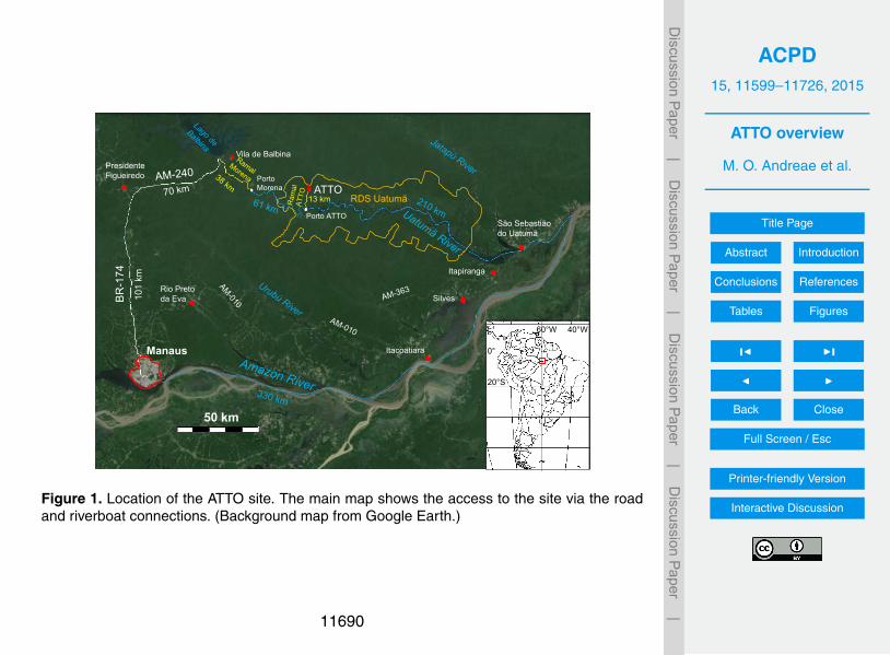
The ATTO site is located 150 km northeast of Manaus in the Uatumã SustainableDevelopment Reserve (USDR) in the Central Amazon (Fig. 1). In a workshop on 23June 2009 in Manaus, Brazilian and German Scientists evaluated three potential sites5
in terms of logistical and scientific criteria and decided to establish ATTO in the USDR.This conservation unit is under the control and administration of the Department of En-vironment and Sustainable Development of Amazonas State (SDS/CEUC). The USDRis bisected by the Uatumã River through its entire NE–SW extension. The climate istropical humid, with mean annual temperature of 28 ◦C and mean annual precipitation10
of 2376 mm (IBGE, 2012). The region is characterized by a pronounced rainy seasonfrom February to May and a drier season from June to October (IDESAM, 2009).
The USDR consists of several different forested ecosystems. The tower site is lo-cated approximately 12 km NE of the Uatumã River, where dense, non-flooded up-land forests (terra firme) prevail on plateaus at a maximum altitude of approximately15
130 ma.s.l. Seasonally flooded black-water (igapó) forest dominates along the mainriver channel, oxbow lakes, and the several smaller tributaries of the Uatumã River (ap-proximately 25 ma.s.l.). Interspersed with these formations are non-flooded terra firmeforests on ancient river terraces (35–45 ma.s.l.), and campinas (savanna on white-sandsoils) and campinaranas (white-sand forest), which are predominantly located between20
the river terraces and the slope to the plateaus.Upwind of the site in the main wind direction (northeast to east), large areas covered
by mostly undisturbed terra firme forests extend over hundreds of kilometers. To thenortheast, the nearest region with dense human activity is in the coastal regions of theGuyanas and of Amapá State, about 1100 km away. In the easterly direction, the main25
stem of the Amazon is in the fetch region of ATTO, with scattered smaller towns and thecities of Santarém and Belém at distances of about 500 and 900 km, respectively. Tothe southeast, the densely populated states of the Brazilian Nordeste lie at distances
greater than 1000 km. Figure 2 presents on overview of the population density and thedominant land cover in northern South America.
The origins of the predominant airmasses at ATTO change throughout the year, asthe Intertropical Convergence Zone (ITCZ) undergoes large seasonal shifts over theAmazon Basin, resulting in pronounced differences in meteorological conditions and5
atmospheric composition (Andreae et al., 2012). This is illustrated in Fig. 3, whichshows monthly trajectory frequency plots for 9 day backtrajectories arriving at ATTO atan elevation of 1000 m. During boreal winter, the ITCZ can lie as far south as 20◦ S,so that a large part of the Basin, including ATTO, is in the meteorologically North-ern Hemisphere (NH). Airmasses then arrive predominantly from the northeast over10
a clean fetch region covered with rain forest. During this period, long-range transportfrom the Atlantic and Africa brings episodes of marine aerosol, Saharan dust, andsmoke from fires in West Africa. This flow pattern shifts abruptly at the end of May,when the ITCZ moves to the north of ATTO. This shift marks the beginning of the dryseason at ATTO, a period of time during which the site is exposed to airmasses from15
the easterly and southeasterly fetch regions, which receive considerable pollution frombiomass burning and other human activities in northeastern Brazil. In July almost theentire Basin is south of the ITCZ, and thus lies in the Southern Hemisphere (SH) bothmeteorologically and geographically. The transition to the northeasterly flow pattern ismore gradual, beginning in September and becoming complete only in March.20
2.2 Access
The ATTO site is reached from Manaus by following national highway BR-174 for101 km northward to a junction south of Presidente Figuereido, then heading 70 km tothe E on a paved side road, AM-240, towards Balbina, then 38 km SE on the dirt roadRamal da Morena along the Uatumã River to the small community of Porto Morena,25
where the road ends. After a 61 km motor-boat ride on the Uatumã River towards theSE the landing, Porto ATTO, is reached. The access road from the landing to the ATTOsite on the plateau follows an old trail used in the 1980s to extract Pau Rosa wood from
the forest. This trail was re-opened in 2010 and widened to an ATV and tractor traffi-cable path that was used during the initial years of the development of the ATTO site.In 2012/13 the government of the State of Amazonia, represented by the Secretariade Estado de Infraestrutura, SEINFRA, financed and implemented a 6 m wide dirt roadbetween the Uatumã River and the ATTO tower site, which accommodates pickups and5
trucks. The overall distance along this road, Ramal ATTO, is 13.7 km, rising from 25 to130 ma.s.l. During the years of the project development, the travel time from Manaushas been gradually reduced from a whole-day trip in 2009 to a 4.5 h ride in 2014. Forthe delivery of large and heavy equipment to Porto ATTO, fluvial transportation by shipor pontoon is possible from Manaus by going down the Amazonas River and up its10
tributary, Rio Uatumã, a distance of ca. 550 km and travel time of 2 days.
2.3 Camp
The base camp on the ATTO plateau was built in 2011/12 by a team of techniciansfrom INPA/LBA and workers hired from the Uatumã Sustainable Development Reserve(USDR). The camp has electrical power and water, and facilities include toilets and15
a dormitory with hammocks that can accommodate ca. 20 people. Another camp isplanned by INPA at the Uatumã River landing, which will serve also as a base stationfor ecological research in the area. A helicopter landing site is intended adjacent to thiscamp.
2.4 Towers20
The measurement facilities on the ATTO plateau consist of two towers of ca. 80 mheight, already implemented, and the 325 m tall tower, whose construction began inSeptember 2014, and is now nearing completion. In 2010, an 81 m triangular mast wasestablished for pilot measurements, which is currently used for a wide set of aerosolmeasurements, followed in 2011 by an 80 m heavy-duty guy-wired walk-up tower, pur-25
chased from the Irish company UPRIGHT (formerly INSTANT). The walk-up tower can
carry a total payload of 900 kg, with outboard platforms on 5 levels. It is currently usedfor meteorological and trace gas measurements. The measurements at the top level, at79.3 m, are the highest ground based measurements within the Amazonian rain forestperformed so far. The tower coordinates (WGS 84) are given in Table 1. The measuringinstruments are accommodated in three air-conditioned containers, the trace gas lab5
and the greenhouse gas lab at the base of the walk-up tower, and the aerosol lab at thebase of the mast, each lab with inside dimensions of 292×420×200 cm (W×L×H)and supplied by 230/135 V electrical power.
2.5 Communications
Since the end of 2013, the ATTO site has been connected to the internet by satel-10
lite. The uplink is realized by the mobile satellite terminal Cobham EXPLORER 700using the INMARSAT/BGAN broadband network, providing a data bandwidth of up to492 kbps. Operating in the L-Band, its active antenna performance allows up to 20 dBcompensation of signal attenuation due to bad weather. The antenna is mounted at50 m height on the walk-up tower, aligned by 43.9◦ elevation and 273.1◦ azimuth to-15
wards the geostationary satellite INMARSAT 4-F3 Americas.A cluster of two redundant routers manages the internet traffic and provides direct
access from the internet to the various computers and networkable instruments at theATTO site. The routers are providing additional features like centralized data storage,remote server access, optimized file transfer, monitoring systems, updating clients,20
VoIP telephony between the local infrastructural sites, etc. Internal data communicationbetween the various sites on the ATTO plateau (towers, labs, camp) is realized viaa wireless LAN bridge, operating in the 5 GHz mode, featured by access points withdirected-beam antennas.
Data communication within each site occurs via wired LAN with data rates of up to25
1000 kbps. In addition, at the camp there is WLAN available in the 2.4 GHz mode. Thecommunication system allows monitoring and controlling of networkable instrumentsin all three lab containers, as well as internet e-mailing, locally and globally. For oral
communication with the remote ATTO site and for safety matters, satellite phones (Isat-PhonePro) are available operating in the INMARSAT net.
2.6 Electrical power supply
Electrical power is provided by a system of diesel generators. Currently, the scientificsites (lab containers and towers) are supplied by two 60 Hz generators with 45 and 405
kVA, operating alternately by weekly switching. They are located ca. 800 m downwindfrom the measuring sites to avoid contamination. Due to the long distance betweenpower generation and consumption, power is transmitted via two 600 V transformers,using two parallel cables, each 3mm×16mm. The voltage provided to the labs is 230and 135 V, and UPSs are being used to stabilize energy. Power to the camp is provided10
separately to avoid power fluctuations at the measurement sites. When the tall toweris established, it is planned to upgrade the power generation to a new system of 2×100 kVA generators at a distance of 2–3 km downwind of the tower.
3 Measurement methods
3.1 Floristic composition and biomass characterization15
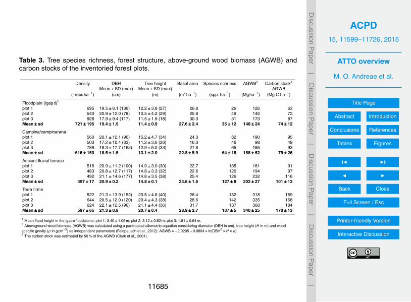
Forest plots of three ha each were inventoried in the igapó, the campinarana, the terrafirme on ancient river terraces, and the terra firme on the plateau, in order to providea preliminarily description of the floristic composition and turnover as well as the above-ground wood biomass (AGWB) in the different forested ecosystems near the tower site.All trees with ≥ 10 cm DBH (diameter at breast height) were numbered, tagged with alu-20
minum plates, and, when possible, identified in the field. Fertile and sterile voucherswere collected for later identification in the INPA herbarium, Manaus. The AGWB wasestimated by a pantropical allometric model (Feldpausch et al., 2012) considering DBH,tree height, and wood specific gravity. We measured tree height with a trigonometricmeasuring device (Blume–Leiss) and determined wood specific gravity by sampling25
cores from the tree trunk and calculating the ratio between dry mass (after drying thewood samples at 105 ◦C for 72 h) and fresh volume. Additionally we used data from theGlobal Wood Density Database DRYAD (Chave et al., 2009) for tree species withoutdetermined wood specific gravity in the terra firme forests and from Targhetta (2012)for tree species in the campina and igapó forests.5
3.2 Meteorology
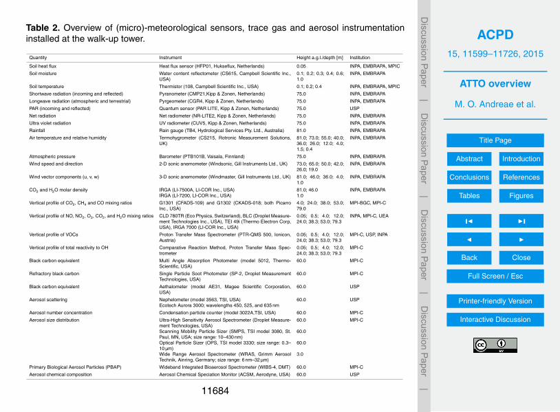
The walk-up tower is equipped with a suite of standard meteorological sensors (includ-ing vertical profiles, for details see Table 2). The following quantities are continuouslyrecorded: (a) soil heat flux, soil moisture and soil temperature (10 min time resolu-tion), (b) incoming and outgoing short and long wave radiation, photosynthetic active10
radiation (PAR), net radiation, ultraviolet radiation, rainfall, relative humidity (RH), airtemperature, atmospheric pressure, wind speed and direction (1 min time resolution).Data acquisition is realized by several data loggers (CR3000 and CR1000, CampbellScientific Inc., USA). Visibility is measured with an optical fog sensor (OFS, EigenbrodtGmbH, Königsmoor, Germany), which detects the backscattered light intensity from15
a 650 nm laser.
3.3 Turbulence and flux measurements
Turbulent exchange fluxes of H2O and CO2 as well as surface boundary layer stabilityare measured within and above the canopy using the eddy covariance (EC) technique.The method is well documented in the literature (e.g., Baldocchi, 2003; Foken et al.,20
2012) and will not be described here. Three-dimensional wind and temperature fluctua-tions were measured by sonic anemometers at 81.0, 46.0 and 1.0 ma.g.l. (see Table 2).CO2 and H2O fluctuations are detected by three fast response open-path CO2/H2O in-frared gas analyzers installed at a lateral distance of about 10 cm from the sonic path.The high-frequency signals are recorded at 10 Hz by CR1000 data loggers. The raw25
data are processed applying state-of-the-art correction methods using the software
Alteddy (version 3.9) based on Aubinet et al. (2000). Detailed information about thissoftware is available in the internet (www.climatexchange.nl/projects/alteddy/). Fluxes,means and variances were calculated for half-hourly intervals (de Araújo et al., 2002,2008, 2010).
3.4 Vertical profiles of reactive trace gases and total OH reactivity5
Ozone is measured by a UV-absorption technique with a Thermo Scientific 49i analyzer(Thermo Scientific, Franklin, MA, USA), using Nafion dryers to minimize the effects ofchanging water vapor concentrations, as suggested by Wilson and Birks (2006). Mixingratios of CO2 and H2O are measured by non-dispersive infrared absorption techniques(Licor-7000, LI-COR, Lincoln, USA).10
During intensive campaigns, measurements of mixing ratios of Volatile Organic Com-pounds (VOC), total OH reactivity, nitric oxide (NO), nitrogen dioxide (NO2), ozone(O3), and water vapor (H2O) were carried out at 8 heights, in and above the rain forestcanopy, using a reactive trace gas profile system similar to that described by Rummelet al. (2007). The lower part of the vertical profile (0.05, 0.5, and 4 m above the forest15
floor) was set up at an undisturbed location near the walk-up tower (distance 12 m).The upper part of the vertical profile (12, 24, 38, 53, and 79 m above forest floor) wasmounted on the north-west corner of the walk-up tower. Heated and insulated intakelines (PTFE) were fed to the analyzers, which were housed in the air conditioned labcontainer 10 m west of the walk-up tower.20
The NO mixing ratio was determined by a gas-phase chemiluminescence technique(NO Chemiluminescence analyzer, model CLD TR-780, Ecophysics, Switzerland). Themixing ratio of NO2 was determined by the same analyzer after specific conversionto NO by a photolytic converter (Solid-state Photolytic NO2 Converter (BLC); DMT,Boulder/USA).25
Measurements of Volatile Organic Compounds (VOC) were performed using a Pro-ton Transfer Reaction Mass Spectrometer (PTR-MS, Ionicon, Austria) operated understandard conditions (2.2 hPa, 600 V, 127 Td; 1 Td= 10−21 Vm2.). The instrument is ca-
pable of continuously monitoring VOCs with proton affinities higher than water andat low mixing ratios (several ppt with a time resolution of about 1–20 s). The protontransfer reaction is a soft chemical ionization technique, meaning that fractionation ofcompounds is low. More detailed information is provided elsewhere (Lindinger et al.,1998). Protonated water molecules H3O+ are used to charge the compound of interest5
prior to separation and detection by a quadrupole mass spectrometer according to theirmass to charge ratio. One entire VOC vertical profile (from 0.05 to 80 m, 8 heights intotal) can be determined every 16 min using the same inlet system as the NO, NO2,O3, and CO2 instruments.
Calibration was performed using a gravimetrically prepared multicomponent stan-10
dard (Ionimed, Apel&Riemer). Occasionally, samples were collected in absorbentpacked tubes (130 mg of Carbograph 1 [90 m2 g−1] followed by 130 mg of Carbograph5 [560 m2 g−1]; Lara s.r.l., Rome, Italy) (Kesselmeier et al., 2002) and analyzed by GC-FID in order to cross-validate the measurements by PTR-MS and to determine themonoterpene speciation for the total OH reactivity measurement.15
In addition to the measurement of individual reactive inorganic trace gases and theVOCs, the total OH reactivity was monitored. Total OH reactivity is the summed lossrate of all OH-reactive molecules (mixing ratio× reaction rate coefficient) present in theatmosphere. Comparison of the directly measured total OH reactivity to the summedOH reactivity of the individually detected species allows quantification of the “missing20
or unmeasured” OH reactivity. Direct measurements of total OH reactivity were con-ducted by the Comparative Reactivity Method (Sinha et al., 2008) using a PTR-MS asa detector. The PTR-MS monitored the mixing ratio of a reagent (pyrrole) after mix-ing and reaction in a Teflon-coated glass reactor. Pyrrole first reacts with OH aloneand then with OH in the presence of ambient air containing many more OH reactive25
compounds. The competitive reactions of the reagent and the ambient OH reactivemolecules cause a change in the detected levels of pyrrole. This can be equated to theatmospheric total OH reactivity provided the instrument is well calibrated and appropri-ate corrections are applied (Nölscher et al., 2012). The total OH reactivity instrument
was regularly tested for linearity of response using an isoprene gas standard (Air Liq-uide). VOC and total OH reactivity measurements were performed simultaneously withtwo separate PTR-MS systems measuring from the same inlet, so that the results maybe directly compared over time, height, and season.
3.5 Vertical profiles of long-lived trace gases (CO, CO2, and CH4)5
In March 2012, continuous and high precision CO2/CH4/CO measurements were es-tablished in an air-conditioned container at the foot of the 80 m tall walk-up tower. Thesample air inlets are installed at five levels: 79, 53, 38, 24, and 4 m above ground. Theinlet tubes are constantly flushed at a flow rate of several liters per minute to avoidwall interaction within the tubing. A portion of the sample air is sub-sampled from the10
high flow lines at a lower flow rate for analysis with instruments based on the cavityring-down spectroscopy technique. The G1301 and G1302 Picarro analyzers (PicarroInc., USA) are used for measuring CO2/CH4 and CO/CO2, respectively. Although bothanalyzers also measure the H2O concentration in air, these measurements are not cal-ibrated and can therefore be regarded only as informative.15
The G1301 analyzer provides data with a SD of the raw data below 0.05 ppm forCO2 and 0.5 ppb for CH4, the long-term drift is below 2 ppm and 1 ppbyear−1 for CO2and CH4, respectively. For the G1302, tests with a stable gas tank show a SD of theraw data of 0.04 ppm for CO2 and 7 ppb for CO. The long-term drift of the analyzeris below 2 ppm and 4 ppbyear−1 for CO2 and CO, respectively. Both analyzers agree20
well with a CO2 difference below 0.02 ppm. When the G1301 analyzer broke down in2012, it was replaced from December 2012 until October 2013 by a Fast GreenhouseGas Analyzer (FGGA) based on Off-Axis Integrated Cavity Output Spectroscopy (OA-ICOS; Los Gatos Research Inc., USA) as an emergency solution. This CO2/CH4/H2Oanalyzer is designed for measuring at rates of ≥ 10 Hz and is primarily used for eddy25
covariance and chamber flux measurements where a low drift rate is less vital than forhighly precise and stable long-term measurements. The FGGA operates with a raw SDof 0.6 ppm for CO2 and 2 ppb for CH4; the drift is quite large with 1 ppm and 3 ppbday−1
for CO2 and CH4, respectively. For the time when the FGGA was used, the calibrationand drift correction routines were adopted accordingly. The detailed description of thewhole measurement system, including measurement, calibration and correction rou-tines will be presented elsewhere.
3.6 Aerosol measurements5
3.6.1 Size distributions and optical measurements
Aerosols are sampled above the canopy at 60 m height, without size cut-off, and trans-ported in a laminar flow through a 2.5 cm diameter stainless steel tube into an air-conditioned container (aerosol lab at mast, see Sect. 2.4). The sample humidity is keptbelow 40 % using silica diffusion driers. Since January 2015, the aerosol sample air10
has been dried using a fully automatic silica diffusion dryer, developed by the Institutefor Tropospheric Research, Leipzig, Germany (Tuch et al., 2009). Aerosol size distribu-tions are currently measured from 10 nm up to 10 µm using three instruments: a Scan-ning Mobility Particle Sizer (SMPS, TSI model 3080, St. Paul, MN, USA; size range:10–430 nm), an Ultra-High Sensitivity Aerosol Spectrometer (UHSAS, DMT, Boulder,15
CO, USA; size range: 60–1000 nm), and an Optical Particle Sizer (OPS, TSI model3330; size range: 0.3–10 µm). The SMPS provides an electromobility size distribution,whereas the UHSAS and OPS measure aerosol light scattering and estimate the sizedistributions from the particle scattering intensity (Cai et al., 2008). In addition to thecontinuous above-canopy size measurements, aerosol size distributions are measured20
with the Wide Range Aerosol Spectrometer (WRAS, Grimm Aerosol Technik, Ainring,Germany; size range: 6 nm–32 µm) from a separate inlet line below the canopy at 3 mheight. The WRAS provides electromobility size distributions in the size range of 6–350 nm and uses particle light scattering for the size range above 300 nm. Details ofthe instrumentation setup are given in Table 2.25
For measuring aerosol light scattering, we use a three-wavelength integrating neph-elometer (until February 2014: TSI model 3563, wavelengths 450, 550, and 700 nm;
after February 2014: Ecotech Aurora 3000, wavelengths 450, 525, and 635 nm) (An-derson et al., 1996; Anderson and Ogren, 1998). Calibration is carried out using CO2as the high span gas and air as the low span gas. The zero signals are measured onceevery twelve hours using filtered ambient air. Noise level and detection limits for the TSI3563 have been investigated by Anderson et al. (1996). At low particle concentrations5
and/or short sampling times, random noise dominates the nephelometer uncertain-ties. For the 300 s averages applied here, the detection limits, defined as a signal tonoise ratio of 2, for scattering coefficients are 0.45, 0.17, and 0.26 Mm−1 for 450, 550,and 700 nm, respectively. Since sub-micrometer particles predominate in the particlenumber size distribution at our remote continental site, the sub-micron (as opposed to10
super-micron correction or an average of the two) corrections given in Table 4 of An-derson and Ogren (1998) were used for the truncation corrections. Bond et al. (2009)suggested that this correction is accurate to within 2 % for a wide range of atmosphericparticles, but that the error could be as high as 5 % for highly absorbing particles.
A Multi-Angle Absorption Photometer (MAAP, Carusso/Model 5012 MAAP, Thermo15
Electron Group, USA, λ = 670 nm) and a 7-wavelength Aethalometer (until Jan-uary 2015 model AE-31, since then model AE33) (Magee Scientific Company, Berke-ley, CA, USA, λ = 370, 470, 520, 590, 615, 660, 880, and 950 nm) are used for measur-ing the light absorption by particles. The MAAP and aethalometer have been deployedat ATTO since March 2012. In the MAAP instrument, the optical absorption coefficient20
of aerosol collected on a filter is determined by radiative transfer calculations, whichinclude multiple scattering effects and absorption enhancement due to reflections fromthe filter. A mass absorption efficiency (αabs) of 6.6 m2 g−1 was used to convert theMAAP absorption data to equivalent BC (BCe). For the Aethalometer, an empirical cor-rection method described by Rizzo et al. (2011) was used to correct the data for the25
scattering artifact.Biological material is measured with the Wideband Integrated Bioaerosol Spectrom-
eter (WIBS-4, DMT). The WIBS utilizes light-induced fluorescence technology to detectbiological materials in real-time based on the presence of fluorophores in the ambient
particles (Kaye et al., 2005). A 2×2 excitation (280 and 370 nm)-emission (310–400and 420–650 nm) matrix is recorded along with the particle optical size and shapefactor.
3.6.2 Chemical measurements and hygroscopicity
The submicron non-refractory aerosol composition is measured using an Aerosol5
Chemical Speciation Monitor (ACSM, Aerodyne, USA) as described by Ng et al. (2011).The instrument is a compact version of the widely used Aerodyne Aerosol Mass Spec-trometer (Jayne et al., 2000). The ACSM efficiently samples aerosol particles throughan aerodynamic lens in the 75–650 nm size range and characterizes the mass andchemical composition of the non-refractory species. The focused particle beam is10
transmitted into a detection chamber where the non-refractory fraction flash vapor-izes on a hot surface (typically at 600 ◦C). Subsequently, the evaporated gas phasecompounds are ionized by 70 eV electron impact and their spectra determined usinga quadrupole mass spectrometer. The chemical speciation is determined via decon-volution of the mass spectra according to Allan et al. (2004). Mass concentrations of15
particulate organics, sulfate, nitrate, ammonium, and chloride are obtained with detec-tion limits< 0.2 µgm−3 for 30 min of signal averaging. Mass calibration of the systemis performed using size-selected ammonium nitrate and ammonium sulfate aerosol fol-lowing the procedure described by Ng et al. (2011). A collection efficiency (CE) of 1.0 isapplied (similar to Chen et al., 2015), yielding good agreement with other instruments.20
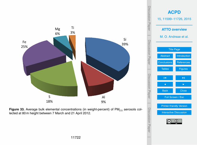
PM2.5 sampling was carried out from 7 March to 21 April 2012 on Nuclepore® poly-carbonate filters at 80 m on the walk-up tower using a Harvard Impactor; samples werecollected over 48 h periods. They were analyzed by Energy-Dispersive X-ray Fluores-cence (EDXRF) (PANanytical, MiniPal4) at 1 mA and 9 kV for low-Z (Na to Cl) elements,and 0.3 mA, 30 kV, and internal Al filter for the other elements. Soluble species were25
determined by Ion Chromatography (Dionex, ICS-5000) using conductivity detectionfor cations and anions and UV-VIS for soluble transition metals. For cation separation,
the capillary column CS12A was used, for anions, an AS19 column, and for transitionmetals, a CS5A column (calibrated to quantify traces of Fe2+ and Fe3+).
Size-resolved cloud condensation nuclei (CCN) measurements are performed us-ing a continuous-flow streamwise thermal gradient CCN counter (CCNC), commer-cially available from Droplet Measurement Technologies, Inc. (model CCN-100, DMT,5
Boulder, CO, USA), a differential mobility analyzer (DMA, Grimm Aerosol Technik, Ain-ring, Germany) and a condensation particle counter (CPC model 5412, Grimm AerosolTechnik). By changing the temperature gradient, the supersaturation of the CCNC isset to values between 0.1 and 1.1 %. Particles with a critical supersaturation equal toor smaller than the prescribed supersaturation (Spresc) are activated and form water10
droplets. The completion of a full measurement cycle comprising CCN efficiency spec-tra at 10 different supersaturation levels takes ∼ 4 h. The measurement period alreadycovers 12 months and is being continued. The long-term data set provides unique infor-mation on the size dependent hygroscopicity of Amazonian aerosol particles through-out the seasons. The results will complement and extend the results from previous15
campaigns (e.g., Gunthe et al., 2009; Rose et al., 2011; Levin et al., 2014).
3.6.3 Microspectroscopic analysis of single aerosol particles
Complementary to the online long-term aerosol measurements, modern offline tech-niques were applied to aerosol samples collected at the ATTO site. In particular, mi-crospectroscopic techniques, such as Scanning Transmission X-ray Microscopy with20
Near-Edge X-ray Absorption Fine Structure Analysis (STXM-NEXAFS) and ScanningElectron Microscopy with Energy Dispersive X-ray spectroscopy (SEM-EDX), were uti-lized to shed light on the morphology and composition of single aerosol particles withnanometer resolution.
Aerosol samples for Scanning Electron Microscopy with Electron Probe Micro-25
analysis (EPMA) were collected at the ATTO site on top of the 80 m tower in April 2012.For the collection of size-segregated samples for single particle (i.e., EPMA) analysis,
we used a Battelle impactor with aerodynamic diameter cut-offs at 4, 2, 1 and 0.5 µm.The particles were collected on TEM grids covered with a thin carbon film (15–25 nm).
Aerosol samples for x-ray microspectroscopy were collected using a homemade sin-gle stage impactor, which was operated at a flow rate of 1–1.5 Lmin−1 and a corre-sponding 50 % size cut-off of about 500 nm. Particles below this nominal cut-off are not5
deposited quantitatively; however, a certain fraction is still collected via diffusive depo-sition and therefore available for the STXM analysis. Aerosol particles were collectedonto silicon nitride substrates (Si4N3, membrane width 500 µm, membrane thickness100 nm, Silson Ltd., Northhampton, UK) for short sampling periods (∼ 20 min), whichensures an appropriately thin particle coverage on the substrate for single particle anal-10
ysis. Detailed information can be found in Pöhlker et al. (2012, 2014).STXM-NEXAFS is a synchrotron-based technique and measurements were
made at the Advanced Light Source (ALS, Berkeley, CA, USA) and the BerlinerElektronenspeicherring-Gesellschaft für Synchrotronstrahlung (BESSY II, Helmholtz-Zentrum Berlin für Materialien und Energie (HZB), Germany). A detailed description15
of the instrumentation can be found elsewhere (Kilcoyne et al., 2003; Follath et al.,2010). In the soft X-ray regime, STXM-NEXAFS is a powerful microscopic tool withhigh spectroscopic sensitivity for the light elements carbon (C), nitrogen (N), and oxy-gen (O) as well as a variety of other atmospherically relevant elements (e.g., K, Ca, Fe,S, Na). The technique allows analyzing the microstructure, mixing state, as well as the20
chemical composition of individual aerosol particles.The SEM/EDX analysis was carried out using a Jeol JSM-6390 SEM equipped with
an Oxford Link SATW ultrathin window EDX detector. For EPMA, quantitative and qual-itative calculations of the particle composition were performed using iterative MonteCarlo simulations and hierarchical cluster analysis (Ro et al., 2003) to obtain average25
relative concentrations for each different cluster of similar particle types.
3.6.4 Chemical composition of secondary organic aerosol
Filter sampling for Secondary Organic Aerosol (SOA) analysis was performed on thewalk-up tower at a height of 42 m above ground level. Fine aerosol (PM2.5) was sampledat a flow rate of 2.3 m3 h−1 on TFE coated borosilicate glass fiber filters (PALLFLEX,T60A20, Pall Life Science, USA). The sampling times were 6, 12, or 24 h. After sam-5
pling the filters were stored at 255 K until extraction.The extraction of the filters was performed with acetonitrile (≥ 99.9 %; Sigma Aldrich)
in a sonication bath at room temperature. The filter extracts were evaporated witha gentle nitrogen flow at room temperature in an evaporation unit (Reacti Vap 1; FisherScientific), and the residue was re-dissolved in 100 µL HPLC grade water (Milli-Q water10
system, Millipore, Bedford, USA)/acetonitrile (≥ 99.9 %; Sigma Aldrich) mixture (8 : 2).The separation and analysis was performed with an UHPLC-system (Dionex Ulti-
Mate 3000 series, auto sampler, gradient pump and degasser) coupled to a Q Exac-tive electrospray ionization Orbitrap mass spectrometer (Thermo Scientific). A HypersilGold column (50mm×2.1mm, 1.9 µm particle size, 175 Å pore size; Thermo Scientific)15
was used. The eluents were HPLC grade water (Milli-Q water system, Millipore, Bed-ford, USA) with 0.01 % formic acid and 2 % acetonitrile (eluent A) and acetonitrile with2 % HPLC grade water (eluent B). The flow rate of the mobile phase was 0.5 mLmin−1.The column was held at a constant temperature of 298 K in the column oven. The MSwas operated with an auxiliary gas flow rate of 15 (instrument specific arbitrary units,20
AU), a sheath gas flow rate of 30 AU, a capillary temperature of 623 K, and a sprayvoltage of 3000 V. The MS was operated in the negative ion mode, the resolution was70 000, and the measured mass range was m/z 80–350.
4.1.1 Tree species richness, composition, turnover, and aboveground woodbiomass
In total, 7293 trees≥ 10 cm DBH were recorded in the 12 inventoried 1 ha plots, which5
included 60 families, 206 genera and 417 species. Tree species richness was highestin the terra firme forest on the plateau, followed by the terra firme forest on the fluvialterrace, the campinarana, and the seasonally flooded igapó (Table 3). Floristic similarity(Bray–Curtis index) within plots of the same forest types ranged from 45–65 %, butwas highly variable between different forest types (2–54 %). Accordingly, the species10
turnover across the investigated forest types was high, especially when seasonallyinundated forest plots were compared to their non-flooded counterparts (Fig. 4). AGWBvaried considerably between the studied forest ecosystems as a result of varying treeheights, DBH and basal area (Table 3). Carbon stocks in the AGWB increased from74±12 Mgha−1 in the igapó forest to 79±26 Mgha−1 in the campina/campinarana,15
and 101±13 Mgha−1 on the ancient fluvial terrace, reaching maximum values of 170±13 Mgha−1 in the terra firme forests. Tree species richness correlated significantly withcarbon stocks in AGWB (n = 12; r2 = 0.61; p < 0.01).
The floristic data indicate that the rain forests at the ATTO site combine high alphadiversity with high beta diversity at a small geographic scale, where tree species seg-20
regate mainly due to contrasting local edaphic conditions (e.g., Tuomisto et al., 2003;ter Steege et al., 2013; Wittmann et al., 2013). Biomass and C-stocks vary consider-ably between habitats, and show low values upon flooded and nutrient-poor soils andhigh values upon well-drained upland soils, as previously reported elsewhere for otherAmazonian regions (e.g., Chave et al., 2005; Malhi et al., 2006; Schöngart et al., 2010).25
We investigate the potential of cryptogamic covers to serve as a source of bioaerosolparticles and chemical compounds. Cryptogamic covers comprise photoautotrophiccommunities of cyanobacteria, algae, lichens, and bryophytes in varying proportions,which may also host fungi, other bacteria and archaea (Elbert et al., 2012). A common5
feature of all these organism groups is their poikilohydric nature, meaning that theirmoisture status follows the external water conditions. Thus the organisms dry out underdry conditions, being reactivated again upon rain, fog, or condensation.
Starting in September 2014, we have conducted long-term measurements to moni-tor the activity patterns of cryptogamic covers at four different canopy heights at 10 min10
intervals, in which we measure temperature and water content within and light intensi-ties directly on top of biocrusts growing on the trunk of a tree. The activation patternsof cryptogamic covers upon dewfall will be of particular interest to check for correla-tion with patterns of particle release. In on-site measurements cryptogamic covers areanalyzed for their release of biogenic aerosols (e.g., spores). These particles will be15
investigated and compared with results from offline and online aerosol measurementsat the ATTO site.
4.2 Meteorological conditions and fluxes
An overview of the climatic characteristics of the Amazon Basin has been presentedby Nobre et al. (2009). The meteorological setting of the ATTO site has been described20
in Sect. 2.1, and the basic meteorological measurements (wind, temperature, humid-ity, radiation, etc.) at the site reflect the regional climate and the micrometeorologicalconditions influenced by local topography and vegetation. In the following sections wepresent overviews of meteorological observations that characterize the site and initialresults of micrometeorological investigations at ATTO. Since the quantification of the25
exchange of trace gases and aerosols between the rain forest and the atmosphere is
a key objective of the ATTO program, the study of the structure and behavior of theatmospheric boundary layer is a central focus here.
4.2.1 Wind speed and direction above the forest canopy
The wind roses for the dry season (15 June–30 November) and the wet season (1December–14 June) (based on half-hourly averages of wind speed and direction mea-5
sured at 81 ma.g.l. for the period from 18 October 2012 to 23 July 2014; Fig. 5) indicatethe dominance of easterly trade wind flows at the measurement site. A slight shift ofthe major wind direction towards ENE is observed during the wet season, while flowsare mainly from the east during the dry season. This seasonality can be explained bythe inter-annual north–south migration of the Intertropical Convergence Zone (ITCZ),10
which also governs the amount of rainfall (see Poveda et al., 2006). The variation of thewind roses between daytime and nighttime was insignificant. Maximal wind speeds ob-served at the site are about 9 ms−1. The influence of river and/or lake breeze systemscaused by the Rio Uatumã (∼ 12 km distance) or Lake Balbina (∼ 50 km distance) andother thermally driven mesoscale circulations is of minor importance. This shows that15
the sampled air masses mainly have their origin within the fetch of the green oceanextending several hundred kilometers to the east of the site.
4.2.2 Temperature, precipitation, and radiation
As is typical for the central Amazon Basin, the mean air temperature does not showstrong variations at seasonal timescales due to the high incident solar radiation20
throughout the year (Nobre et al., 2009). Climatologically in the Manaus region, thehighest temperatures are observed during the dry season, with a September monthlymean of 27.5 ◦C, whereas the lowest temperatures prevail in the rainy season, witha monthly mean of 25.9 ◦C in March.
Vertical profiles of temperature show clear diurnal cycles driven by radiative heating25
of the canopy during the day and radiative cooling of the canopy and the forest floor
during the night (Fig. 6). Therefore, both temperature minima and maxima are observedat the canopy top during both seasons. A second temperature minimum during nightcan be observed at the forest floor during the dry and wet season. During the daywarm air from above the canopy is transported into the forest. Minimum temperaturesat the canopy top are around 22.5 ◦C during both seasons, whereas daytime maxima5
are around 28 ◦C during the wet season and may reach slightly above 30 ◦C in the dryseason.
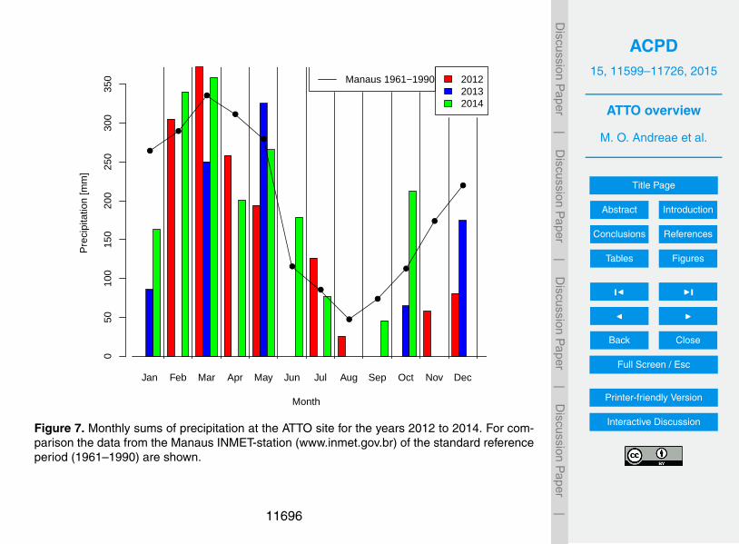
Rainfall in the Manaus region shows a pronounced seasonal variation, reaching thehighest amounts in March (335.4 mm) and the lowest amounts in August (47.3 mm), foran annual total of 2307.4 mm at the INMET station in Manaus for the standard reference10
period 1961 to 1990 (www.inmet.gov.br). Precipitation at the ATTO site follows thisseasonal cycle with maximum values around March and minimum values in Augustand September (Fig. 7). The interannual variability appears to be high all year, butespecially in the transition to the rainy season, a fact that has also been evident in thedata from the years 1981 to 2010 at the Manaus station (Fernandes, 2014). Therefore,15
the large deviations from the regional mean during October to January and also inApril, when the ATTO values from the years 2012–2014 differ substantially from thelong term mean of Manaus, are likely the result of interannual variability.
Overall, however, the precipitation patterns at the ATTO site are in good agreementwith its position in the Central Amazon, where the months between February and May20
are the wettest ones. In this period, the ITCZ reaches its southernmost position andacts as a strong driver in convective cloud formation at the equatorial trough. Due tothe interaction of trade winds and sea breeze at the northeast Brazilian coastline, theITCZ also takes part in the formation of instability lines that enter the continent andregenerate during their westerly propagation. In this way, they account for substantial25
amounts of precipitation. After this period, the ITCZ shifts to the Northern Hemisphere,accompanying the movement of the zenith position of the sun. This leads to less pre-cipitation at the ATTO site, with the driest months being between July and September,when precipitation is formed mostly by local convection. In the following months, the
amount of precipitation increases again, which coincides with the formation of a cloudband in a NW/SE direction that is linked to convection in the Amazon due to the SouthAtlantic Convergence Zone (SACZ) (Figueroa and Nobre, 1990; Rocha et al., 2009;Santos and Buchmann, 2010).
The radiation balance at ATTO as well as the albedo presents a clear difference5
between the wet and the dry seasons. Some episodes when the incident solar radia-tion exceeds the top of atmosphere radiation have been observed for the ATTO data.They were more frequent during the wet season, probably due to the effect of cloudgap modulation that intensifies the radiation received at the surface by reflection andscattering.10
4.2.3 Roughness sublayer measurements
The measurement of turbulent fluxes over tall forest canopies very often implies thatthese measurements are made in the so-called roughness sublayer (RSL). It is usuallyassumed that the RSL extends to 2 or 3 times the height of the roughness obstacles,h0 (Williams et al., 2007). The roughness sublayer is considered to be a part of the15
surface sublayer of the atmospheric boundary layer, but it is too close to the roughnesselements for Monin Obukhov Similarity Theory (MOST) to hold. Some progress in theparameterization of the RSL has been made in terms of applying correction factors tothe traditional similarity functions of the surface layer (see for example, Mölder et al.,1999, and references therein). However, the universality of such procedures remains20
unknown.In this section, we briefly show strong evidence that a simple adjustment factor that
depends on the factor z/z∗ (where z is the height of measurement and z∗ is the heightof the RSL), as employed by Mölder et al. (1999), is not able to collapse the “variancemethod” dimensionless variables25
where σw is the SD of the vertical velocity, u∗ is the friction velocity, σa is the SD ofa scalar, and a∗ is its turbulent scale (see Eqs. 3 and 4 below). In Eqs. (1) and (2), ζ isthe Obukhov length with a zero-plane displacement height calculated as d0 = 2h0/3,5
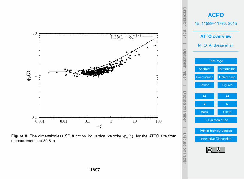
h0 = 40m.We analyzed measurements collected during April 2012 at the 39.5 m level, which is
right at the height of the tree tops, in terms of the turbulent scales
u′w ′ ≡ −u2∗ (3)
and10 ∣∣∣w ′a′∣∣∣ ≡ u∗a∗. (4)
We only analyzed measurements under unstable conditions, and considered onlycases where the sensible heat flux is positive (directed upwards), the latent heat fluxis positive (directed upwards) and the CO2 flux is negative (directed downwards). In(4), the absolute value is used, so that a∗ is always positive. The scalar a represents15
virtual temperature θv (measured by the sonic anemometer), specific humidity q, andCO2 mixing ratio c.
The analysis is made in terms of the dimensionless SD functions φw (ζ ) and φa(ζ )defined above. Overall results for vertical velocity, virtual temperature, and CO2 con-centration are shown in Figs. 8–10. The solid lines in the figures give representative20
functions found in the literature for the surface layer well above the roughness sublayer(see, for example, Dias et al., 2009).
Similar figures were drawn for specific times of day, namely 07:00–09:00, 09:00–11:00, 11:00–13:00, 13:00–15:00 and 15:00–17:00 LT, in an attempt to identify periods
of the day when better agreement (or even a systematic departure, for example bya constant vertical shift) with the surface-layer curves could be identified. Temperatureand humidity are somewhat better behaved in this case, but not CO2, for reasons thatare not clear. Because no conclusive explanation can be found, we do not show theseanalyses here.5
Finally, we tried to apply some concepts recently developed by Cancelli et al. (2012)to relate the applicability of MOST to the strength of the surface forcing. Cancelliet al. (2012) found that the applicability of MOST can be well predicted by their “surfaceflux number”,
Sfa =
∣∣∣w ′a′∣∣∣ (z−d0)
νa∆a, (5)10
where νa is the molecular diffusivity of scalar a in the air, and ∆a is the gradient of itsmean concentration between the surface and the measurement height.
In our case, there is no easy way to obtain ∆a, so instead we use
Sfa =
∣∣∣w ′a′∣∣∣ (z−d0)
νaσa(6)
As a measure of the applicability of MOST, we use the absolute value of the difference15
between the observed value of φa(ζ ) and its reference value for the surface layer, asused by Dias et al. (2009), and shown by the solid lines in Figs. 8–10. The results areshown in Fig. 11. A relatively stronger forcing is clearly related to a behavior that iscloser to that expected by MOST for both temperature and humidity, but not for CO2.This suggests that CO2 presents even greater challenges for our proper understanding20
of its turbulent transport in the roughness sublayer over the Amazon Forest.Ultimately, the lack of conformity to Monin–Obukhov Similarity Theory found in these
investigations (a fact that has been generally observed in the roughness sublayer over11635
other forests) implies that scalar fluxes over the Amazon forest derived from standardmodels, which use MOST, are bound to have larger errors here than over lower vege-tation, such as grass or crops. We can expect this to affect any chemical species, andtherefore the implications for ATTO are quite wide-ranging. On the other hand, oncethe 325 m tall tower is instrumented and operational, a much better picture will emerge5
on the extent of the roughness sublayer and the best strategies to model scalar fluxesover the forest.
4.2.4 Nighttime vertical coupling mechanisms between the canopy and theatmosphere
During daytime, intense turbulent activity provides an effective and vigorous coupling10
between the canopy layer and the atmosphere above it. As a consequence, vertical pro-files of chemical species do not commonly show abrupt variations induced by episodesof intense vertical flux divergence. Accordingly, scalar fluxes between the canopy andthe atmosphere are relatively well-behaved during daytime, so that their inference fromthe vertical profiles of mean quantities can be achieved using established similarity re-15
lationships. At night, on the other hand, the reduced turbulence intensity often causesthe canopy to decouple from the air above it (Fitzjarrald and Moore, 1990; Betts et al.,2009; van Gorsel et al., 2011; Oliveira et al., 2013). In these circumstances, verticalfluxes converge to shallow layers in which the scalars may accumulate intensely overshort time periods. Furthermore, intermittent turbulent events of variable intensity and20
periodicity provide episodic connection between the canopy and the atmosphere. Insome cases, such events may comprise almost the entirety of the scalar fluxes duringa given night.
Nocturnal decoupling occurs rather frequently at the ATTO site, usually punctuatedby intermittent mixing episodes, in agreement with previous studies made over the25
Amazon forest (Fitzjarrald and Moore, 1990; Ramos et al., 2004). During a typical de-coupled, intermittent night, the horizontal wind components are weak in magnitude andhighly variable temporally, often switching signs in an unpredictable manner (Fig. 12).
As a consequence, it is common that winds from all possible directions occur in sucha night. The example from the ATTO site indicates that despite such a large variability,both horizontal wind components are generally in phase above the canopy, from the42 to the 80 m level. Vertical velocity at the 42 m level is highly intermittent, with var-ious turbulent events of variable intensity scattered throughout the night. While being5
less turbulent, the 80 m level is also less intermittent, presenting a more continuousbehavior. The relevance of the intermittent events to characterize canopy-atmosphereexchange becomes clear when one looks at the fluxes of the scalars, such as CO2(Fig. 12, bottom panel). During this night, the majority of the exchange just above thecanopy (42 m) happened during two specific events, at around 02:00 and 03:30 LT.10
A proper understanding of nocturnal vertical profiles and fluxes of scalars above anyforest canopy depends, therefore, on explaining the atmospheric controls on intermit-tent turbulence at canopy level. In the Amazon forest, this necessity is enhanced, asthere are indications that turbulence is more intermittent there, possibly as a conse-quence of flow instabilities generated by the wind profile at the canopy level (Ramos15
et al., 2004). This is corroborated by early observations at the ATTO site, which indi-cated decoupling and intermittency occuring during more than half of the nights.
It is not yet clear what triggers these intermittent events. In general, previous studiesindicate that the more intense events are generated above the nocturnal boundarylayer, propagating from above (Sun et al., 2002, 2004). On the other hand, less intense20
events that occur in the decoupled state have been characterized as natural modesof turbulence variability generated near the surface (Costa et al., 2011). At ATTO, theoccurrence of the highest intensity at 42 m indicates that intermittency is generatedat the canopy level. Is it possible, then, to identify the mechanisms that trigger theiroccurrence?25
Some evidence can be gathered from a spectral decomposition of the turbulent flowat the different observation levels. Although the horizontal velocities in Fig. 12 are highlyin phase between 42 and 80 m, it is clear from this plot that the wind speed is generallyhigher at 80 m, while there are more turbulent fluctuations at 42 m. When these sig-
nals are decomposed in terms of their time scale to provide a turbulent kinetic energy(TKE) spectrum (Acevedo et al., 2014), the more intense turbulence at 42 m appearsas a peak at time scales just greater than 10 s (Fig. 13). At longer time scales, on theother hand, there is a sharp energy increase at 80 m, making this the most energeticlevel for scales larger than 100 s. Such a low-frequency flow at 80 m is characterized5
by the large wind direction variability apparent in Fig. 12. These are non-turbulent flowpatterns that have been recently classified as “submeso” (Mahrt, 2009). Submeso flowhas low intensity, with large and apparently unpredictable temporal variability. It is usu-ally present in the atmospheric boundary layer, becoming dominant in conditions whenthe turbulent scales are highly reduced, such as in the decoupled nocturnal boundary10
layer.Evidence from ATTO indicates that it is possible to associate the intermittent events
at canopy level with the mean wind shear above the canopy. In Fig. 14, it is evident thatthe two intense events at 42 m, around 21:30 and 02:00 LT, are triggered by episodesof intense wind shear between 42 and 80 m. In conditions where the 80 m wind field15
is dominated by submeso processes, such as in the examples in Figs. 12 and 14, it isthis portion of the flow that determines the occurrence of intense wind shear episodes.Furthermore, it is clear from these examples that flow patterns at levels as high as 80 mexert important controls on the exchange of scalars at canopy level. Questions such asthe height variation of submeso flow have yet to be answered. Tall tower observations,20
such as those planned to be carried on at ATTO, are very important to provide thedata for this kind of analysis and to deepen the understanding of exchange processesbetween the canopy and the atmosphere during the calm nights that are common inthe Amazon forest.
4.2.5 Orographically induced gravity waves in the stable boundary layer above25
the Amazon forest
Gravity waves (GWs) may occur in the forest boundary layer during relatively calmnights. Depending on the magnitude of the turbulent drag, they influence the exchange
processes that take place in the stable boundary layer of the atmosphere (Steeneveldet al., 2009). While convective turbulence is the main factor for daytime transport, thisdriving mechanism decays after nightfall. As a result, other physical processes becomerelevant in the stable boundary layer (SBL), such as drainage flow (Sun et al., 2004),vertical divergence of radiation (Drüe and Heinemann, 2007; Hoch et al., 2007), global5
intermittency (Mahrt, 1999), atmosphere–surface interactions (Steeneveld et al., 2008),and GWs (Nappo, 1991; Brown and Wood, 2003; Zeri and Sa, 2011). Internal gravitywaves can be generated by several forcing mechanisms, including sudden changesof surface roughness, topography, convection, terrain undulations, etc. (Nappo, 2002).These features can reallocate energy and momentum and are significant in determin-10
ing atmospheric vertical structure and the coupling of mesoscale to microscale phe-nomena (Steeneveld et al., 2008, 2009). Chimonas and Nappo (1989) showed thatunder typical conditions of the planetary boundary layer, GWs can interact with themean flow resulting in turbulence at unexpected altitudes.
Fast response data of vertical wind velocity, w, and temperature, T , measured in the15
nocturnal boundary layer (NBL) at the ATTO site were analyzed to detect the occur-rence of gravity waves, and to identify under which situations they would be generatedby terrain undulations, using the methodology proposed by Steeneveld et al. (2009).One of the goals of this study is to investigate the structure of turbulence associatedwith the conditions under which GWs would be forced by ground undulations (class I)20
in contrast to those under which GWs would be expected to be forced by other mecha-nisms (class II). To reach this goal, the methodology of Steeneveld et al. (2009), basedon Chimonas and Nappo (1989), has been used to define whether a specific measure-ment belongs to class I or class II, based on the condition:
L2S= N2/U2 −U ′′/U > k2 (7)25
where k is the wave number associated with the ground undulations and L is the Scorerparameter, U is the mean wind speed, and U ′′ is second derivative of the wind speed
where g is the gravity acceleration and ∆zθ/θ is the dimensionless gradient of the5
virtual potential temperature.Two kinds of data were used: topographic and meteorological. A digital topographic
image of the region surrounding the experimental site was used to analyze the featuresof surface undulations and their scales of occurrence, as well as the space-scale anal-ysis by complex Morlet wavelet transforms (Farge, 1992; Thomas and Foken, 2005).10
Local geomorphometric variables were derived from the SRTM (Shuttle Radar To-pographic Mission) data (Valeriano, 2008). These data were refined to 1 arcsecond(∼ 30 m) from the original spatial resolution of 3 arcsecond (∼ 90 m) and are availableon the site www.dsr.inpe.br/topodata/dados.php.
Time series of the vertical wind velocity and of the fast response temperature data15
provided by a sonic anemometer and thermometer were used to detect GWs eventsat a height of 81 m above the ground. The sampling rate of the measured turbulencedata was 10 Hz. Wind speed and temperature vertical profiles were provided by cupanemometer and thermometer measurements, respectively, with a sampling rate of60 Hz for both, making it possible to compute the Brunt–Väisälä frequency, the vertical20
gradients of wind velocity and the Scorer parameter for GW classification (Steeneveldet al., 2009). Data from five nights have been analyzed, consisting of 120 files of 30 mineach between Julian days number 42 and 46 of the year 2012, representing the firstobservational data available from the ATTO site. The analyses were carried out for thetime between 18:00 and 06:00 LT, for each night with available data (Fig. 15).25
Figure 15a shows a topographic image of the experimental site with colors rangingfrom blue to red representing the altimetry values in meters above sea level. The black
points on the axes in Fig. 15b represent the GW events that have been induced by thetopography of the terrain, whereas the gray points represent GW events that have notbeen generated by terrain orography. The results show that a considerable fraction ofthe analyzed situations represents GW induced by terrain undulations. This finding isvery important for the environmental studies that are being carried out at the Uatumã5
site, as it indicates that some mixing characteristics of the nocturnal boundary layerdepend on the characteristics of terrain undulations and therefore change with thewind direction.
4.2.6 Coherent structure time scale above the ATTO site
Coherent structures (CSs) are a ubiquitous phenomenon in the turbulent atmospheric10
flow, particularly over forests (Hussain, 1986). They occur in the roughness sub-layerimmediately above the plant canopy, where the CSs of the scalar signals show a “ramp-like” shape associated with the two-phase movement of sweep and ejection of the flowinteracting with the canopy. Coherent structures play an important role in biosphere–atmosphere exchange processes (Gao and Li, 1993; Serafimovich et al., 2011). There15
is some consensus that CSs are associated with turbulent flows, although there is nofull agreement on the percentage of the turbulent fluxes associated with them (Lu andFitzjarrald, 1994; Thomas and Foken, 2007; Foken et al., 2012). There has been muchresearch on the dominant scale of occurrence of CSs (Collineau and Brunet, 1993;Thomas and Foken, 2005) and the physical mechanisms responsible for their genera-20
tion (Paw U et al., 1992; Raupach et al., 1996; McNaughton and Brunet, 2002; Cam-panharo et al., 2008; Dias Júnior et al., 2013). Considerable research has also beendevoted to the detection of CSs (Collineau and Brunet, 1993; Krusche and Oliveira,2004) and the dissimilarity between CSs associated with the transport of momentumand scalars (Li and Bou-Zeid, 2011). However, many aspects of their occurrence are25
still poorly known, particularly: (i) their vertical variability (Lohou et al., 2000), (ii) themanifestations of their interaction with gravity waves (Sorbjan and Czerwinska, 2013),(iii) the influence of surface heterogeneity on their features, (iv) aspects of their numeri-
cal simulation (Patton, 1997; Bou-Zeid et al., 2004; Dupont and Brunet, 2009; Wan andPorte-Agel, 2011), particularly in the nocturnal boundary layer (Durden et al., 2013; Zil-itinkevich et al., 2013), and (v) implications of the existence of CSs for the chemistry ofthe atmosphere (Steiner et al., 2011; Foken et al., 2012).
A study on the structure of atmospheric turbulence was performed at the ATTO site5
under daytime conditions, with the aim of contributing to the detection of CSs anddeveloping a better understanding of their vertical and temporal variability over a veryuneven terrain covered by primary forest in central Amazonia. Wind, temperature, andhumidity data were obtained using sonic anemometers and gas analyzers, installed at42 and 81 m above ground, as specified in the methods section. The scales of coherent10
structures were determined following the methodology proposed by Thomas and Foken(2005). Figure 16 shows the average duration of CS for horizontal and vertical windvelocities (u, w), temperature (T ), and humidity (q). For the data at 81 m height, theCS of u and w exhibit temporal scales around 46 and 29 s, respectively. For the twoscalars, T and q, the time scales of the CS are about 44 and 55 s, respectively. For the15
height of 42 m the coherent structure time scales of u, w, T , and q were approximatelyequal to 33, 26, 30 s, and 31 s, respectively.
The results revealed that the CS time scale of the vertical wind velocity is oftensmaller than the scales of the horizontal velocity and the scalar properties, for bothlevels. This can be explained by the fact that the scalar spectra exhibit greater similarity20
to the spectra of the horizontal velocity than to the vertical velocity for low frequencies.Another interesting feature is that the temporal scale of the CS for both the wind velocityand scalars are considerably shorter for the data measured at 81 m compared withthose at 42 m, i.e., the region immediately above the forest canopy appears to be underthe influence of a high-pass filter that removes the lower frequency oscillations of the25
turbulent signals (Krusche and Oliveira, 2004; Thomas and Foken, 2005).
4.2.7 Characteristics of the nocturnal boundary layer
The characteristics of the nocturnal boundary layer (NBL) at the ATTO site near theUatumã River were analyzed for the wet and the dry seasons, based on two method-ologies: (i) the thermodynamic classes of the NBL proposed by Cava et al. (2004) and(ii) the turbulence regimes proposed by Sun et al. (2012).5
Cava et al.’s (2004) classification of nocturnal time series is based on the existence ofa dominant pattern in scalar data, such as CO2 concentration, temperature, or specifichumidity. It also takes into account the variability of nocturnal net radiation (Rn), mea-sured at a sufficiently high sampling rate, which allows cloud detection (with passageof clouds being identified by rapid Rn changes greater than 10 Wm−2). Classes (I), (II),10
(III), are defined by atmospheric conditions free of the influence of clouds, which candisturb the stable boundary layer above the forest. The classes are defined as followedby Cava et al. (2004): (I) the occurrence of coherent structures in the form of “ramps”in scalar time series; (II) the presence of sinusoidal signals (“ripples”) that simultane-ously occur in the time series of scalars above the canopy, and which are typical for15
gravity waves; (III) the existence of turbulence fine structure (i.e., according to Cavaet al. (2004), “periods that lack any geometric structure or periodicity in the time se-ries data”). The last two categories, (IV) and (V), of Cava et al.’s classification referto the simultaneous occurrence of clouds and organized movements with variations inRn > 10 Wm−2. They are: (IV) cases where the net radiation induces organized move-20
ments, and (V) those where the change in net radiation is not correlated with changesin organized movements.
The search of parameters to characterize the turbulent regimes of the nocturnalboundary layer is based on Sun et al. (2012). The three turbulent regimes in the NBLare defined as follows: Regime 1 shows weak turbulence generated by local shear25
instability and modulated by the vertical gradient of potential temperature. Regime 2shows strong turbulence and wind speed exceeding a threshold value (Vλ), above whichturbulence increases systematically with increasing wind speed. This describes the
turbulence generated by bulk shear instability, defined as the mean wind speed dividedby the measuring height. In Regime 3, the turbulence occurs at wind speeds lowerthan Vλ, but is associated with occasional bursts of top-down turbulence. In Regimes 1and 2 the scale of turbulent velocity (VTKE) is related to the mean wind velocity, V . Theturbulent velocity, VTKE, is defined as:5
VTKE =[(1/2)
(σ2u +σ
2v +σ
2w
)]1/2(10)
where u, v , and w are the components of the zonal, meridional and vertical winds,respectively, and σ represents the SD of each variable.
We analyzed 53 data files from the wet season and 79 data files collected during thedry season at the ATTO site. Our results show that the prevailing conditions in the NBL10
are represented by Cava’s classes I, II, and V for both wet and dry seasons (Table 4).Furthermore, during the wet season the classes I and V show their highest percentageof occurrence associated with turbulent Regime 3. Class IV is more frequent whenturbulence Regime 1 prevails. For the dry season we observe that turbulent classes I,IV and V occur most frequently in situations associated with Regime 1 (Table 5).15
4.3 Measurements of atmospheric composition
In March 2012, a basic set of measurements (CO, CO2, CH4, and equivalent blackcarbon, BCe) was initiated at the site, which has been running almost continuouslyup to the present. As CO2 and BCe were measured with multiple instruments in par-allel (see Table 2) an almost complete time series since March 2012 is available for20
these quantities. In November 2012, the long-term measurement setup was upgradedto include measurements of ozone, aerosol scattering, aerosol size distribution, andaerosol number concentration. Due to the complex logistics at this remote site, thereare a few larger data gaps in some of these time series, but the datasets are almostcomplete from the middle of May 2013 to November 2013 and from February 2014 to25
now. Furthermore, several intensive campaigns were conducted with additional mea-surements of aerosol properties, VOC, OH reactivity, and NOx.
4.3.1 CO2, CH4, and CO
Figures 17–19 show the diurnal cycles of the vertical distributions of the concentrationsof CO2, CH4 and CO at the ATTO site. CO2 and CO show a nighttime accumulation5
in the sub-canopy space and a corresponding steepening of the vertical concentrationgradient, which is greatly reduced during daytime due to the enhanced vertical mixingthroughout the canopy. In addition, CO2 exhibits a clear minimum during daytime atmid-canopy level induced by photosynthesis. Interestingly, the build-up of the nighttimemaximum of CH4 proceeds from above the canopy (Fig. 18). The origin of this behavior,10
which seems to be linked to multiple processes, is under investigation. During daytimeCO2, CH4 and CO still exhibit a small vertical gradient below the canopy, indicatinga local source near the ground.
Additional evidence for local surface sources are sporadic concurrent increases ofCH4 and CO predominantly on the lowest measurement level. Examples are shown15
in Fig. 20. The origin of this local CH4-CO source is not known. A remote source(e.g., from the large water reservoir behind the Balbina Dam 60 km northwest of ATTO)seems unlikely, as such a signal would be vertically diluted before reaching the ATTOsite. A combustion source also appears unlikely, as the observed CH4/CO ratios areseveral orders of magnitude higher than the values typical of combustion emissions.20
Apart from these CH4/CO peaks, we occasionally observe, mostly during nighttime,short CH4 peaks of up to more than 100 ppb amplitude. These peaks last a few hours,they do not always concur with increases in CO concentrations, and often coincide with“bursts” of particles with a diameter of a few tens of nanometers.
Figure 21 shows the statistics of monthly daytime (defined as between 13:00–25
16:00 LT, or 17:00–20:00 UT) 30 min measurements of CO2 from three levels (4, 38,and 79 m) respectively. The measurements at the 4 m level are consistently higher thanthe upper levels, while the 38 m level consistently shows lower values during daytime
than the top level (79 m). This indicates that photosynthesis is active throughout theyear. The record is still too short to reveal a clear seasonality. Nevertheless, it appearsthat CO2 from June to August is about 5 ppm above the values during the months fromDecember to February.
Statistics of monthly daytime 30 min measurements of CH4 and CO are shown in5
Fig. 22 (from the 79 m level only). Because of a large data gap due to a malfunctioningof the analyzer, a seasonal cycle is not discernible in the present CH4 record. CO doesshow a seasonal cycle at ATTO with concentrations higher by about 50 ppb during thedry months with a significant fraction of air coming from the south-east (see Fig. 3).
Monthly daytime concentrations of CO2, CH4, and CO are compared in Fig. 23 with10
measurements upstream of ATTO: Cape Verde (green symbols) reflecting the southernend of the Northern Hemisphere, and Ascension Island (brown symbols) representingconditions in the Southern Hemisphere. At least during the period of July to December,CO2 concentrations clearly reach lower values than at both upstream locations, re-flecting the regional carbon sink in the Amazon domain. Likewise, CH4 levels at ATTO15
lie almost on Northern Hemisphere levels throughout the year, even when the ITCZ isnorth of ATTO in austral winter and the site is in the atmospheric Southern Hemispherewith its lower background CH4 concentrations. This suggests the presence of regionalCH4 emissions in the airshed of ATTO.
4.3.2 Biogenic volatile organic compounds and OH reactivity20
The first successful vertical gradients of biogenic VOCs and total OH reactivity weremeasured in November 2012 at the walk-up tower using the gradient system asdescribed in Sect. 3.4. Diurnal fluctuations of isoprene are apparent at all heights(Fig. 24). Under daylight conditions, isoprene mixing ratios were always highest at the24 m level, reaching up to 19.9±2.0 ppb (average ±SD) and indicating a source at the25
canopy top. During nighttime, the light-driven emissions of isoprene cease and the in-canopy mixing ratio fell to 1.1±0.5 ppb, which was lower than observed above the forestat 80 m (2.3±0.3 ppb). Measurements in the canopy (24 m) vary by a factor of ten from
day to night, while measurements close to the ground (0.05 m) vary only by a factorof two. This clearly demonstrates a canopy emission of isoprene, with a peak aroundnoon, when light and temperature are at their maximum. Isoprene mixing ratios at theground level were always the lowest, indicating a potential sink at the soil/litter level orrelatively slow downward mixing. A detailed discussion of measurements of isoprene5
and other biogenic VOC at ATTO was published recently (Yañez-Serrano et al., 2014).In November 2012, the high levels of isoprene measured above the canopy con-
tributed significantly (on average about 85 %) to the total OH reactivity. From Fig. 25,it can be seen that median isoprene mixing ratios of between 0.5 ppb at 06:00 LT and8 ppb in the late afternoon above the canopy give an OH reactivity of about 1–20 s−1.10
The gap between the two curves is the fraction of total OH reactivity that is not due toisoprene. For most of the time this gap is small and within the uncertainty of the mea-surements. On two occasions within this dataset from November 2012, however, thetotal OH reactivity was significantly higher than the isoprene contribution, these beingin the early morning (09:00 LT) coincident with a drop in light levels, and in the after-15
noon just after sunset (17:00 LT). For all other times in the course of the day, isoprenewas the major sink for OH above the canopy. Overall a distinct diel variability in total OHreactivity can be observed, similar to that of its major contributor, isoprene. The medianlifetime of OH radicals during the dry-to-wet transition season above the forest canopyat 80 m varied from about 50 ms by day to 100 ms by night. Ongoing measurements20
will determine the seasonal variability in total OH reactivity and the relative contributionof isoprene.
4.3.3 Ozone profiles
The O3 mixing ratios (Fig. 26) show typical diurnal cycles for both seasons, with val-ues increasing from the morning to the afternoon and subsequently decreasing due to25
deposition and chemical reactions. The afternoon O3 maxima at the uppermost height(79 m) are about a factor of 1.4 higher during the dry season than during the wet sea-son, averaging about ∼ 11 and ∼ 8 ppb, respectively. As found in previous studies, its
deposition to surfaces causes O3 to exhibit distinct vertical profiles (Fig. 26), whichmakes a direct intercomparison to other measurements difficult. However, the mixingratios above the canopy from different studies in the Amazonian rain forest are withina narrow range of 7 to 12 ppb (Kirchhoff et al., 1990; Andreae et al., 2002; Rummelet al., 2007; Artaxo et al., 2013) during the wet season. A budget study by Jacob and5
Wofsy (1990) revealed that downward transport of O3 mainly controlled the mixingratios near the surface, with only a minor contribution from photochemical formationabove the canopy. This may explain the similar mixing ratios in the different studies.Furthermore, only small O3 differences were measured between 38 m (just above thecanopy) and the top of the tower at 79 m during the wet season.10
A different picture is observed during the dry season, with much higher O3 mixingratios at more polluted sites (∼ 40 ppb in Rondônia: Kirchhoff et al., 1989; Andreaeet al., 2002; Rummel et al., 2007), which can be related to biomass burning emissionscausing photochemical O3 formation (Crutzen and Andreae, 1990). A site comparableto the ATTO site is the ZF2 site, located about 60 km north-west of Manaus, which has15
been used extensively in the past (Artaxo et al., 2013). At the ZF2 site, mean maximumO3 mixing ratios measured at 39 m from 2009–2012 (Artaxo et al., 2013) match exactlythose measured at the ATTO site for the wet season, but are about a factor of 1.5 higherduring the dry season. This may be attributed to the more pristine character of theATTO site, but could also be related to the different measurement periods or different20
biogenic emissions at the sites. In order to distinguish these different influences, high-quality long-term measurements are required, which are now being generated withinthe ATTO project.
During the wet season, the amplitude of the mean diurnal cycle at 79 m is only about2 ppb, whereas it is 3–4 ppb during the dry season. The highest amplitudes are ob-25
served within the canopy and the understory with up to 5 ppb (24 m) in the dry season.These variations can be attributed to downward mixing of O3, which is “stored” withinthe canopy (so called storage flux, see Rummel et al., 2007). It is subsequently de-pleted by chemical reactions, mostly with soil biogenic NO, and deposition after the
forest canopy becomes decoupled from the atmosphere above at nighttime. During thewet season, the largest decrease in O3 mixing ratios occurs at the canopy top. Thismight be attributed to a lower canopy resistance to O3 deposition due to enhancedstomatal aperture during the wet season as proposed by Rummel et al. (2007) and willbe the subject of future work. Further investigations will also focus on the interactions5
between turbulence (supply of O3) and trace gases that react with O3, especially nitricoxide (NO).
4.3.4 Aerosol optical properties
The aerosol optical properties measured at ATTO are shown as a time series in Fig. 27and summarized in Table 6. The averages were calculated for the dry season, August–10
October, and the wet season, February–May (2012–13 for the absorption measure-ments and 2013 for the scattering measurements). The transition periods betweenthese two seasons are not included in the summary, in order to show the contrast be-tween the cleanest and “more polluted” periods. The scattering coefficients are similarto those reported by Rizzo et al. (2013) from measurements performed at the ZF2 site15
(60 km N of Manaus). The regional transport of biomass burning emissions is the mainsource of particles during the dry season. Its influence is significant, as can be seen bycomparing the scattering and absorption coefficients from both seasons, which aver-age about 3–6 times higher during the dry than during the wet season. During the wetseason, ATTO is meteorologically located in the NH and the scattering and absorption20
coefficients reach their minimum values, however, some episodes of long-range trans-port of aerosols from the ocean and Africa still lead to episodically elevated values.
The contrast between the wet and dry seasons can be attributed to a combinationof higher removal rates by wet deposition during the wet season and the dominantinfluence from biomass burning and fossil fuel emissions during the dry season, which25
are the main sources of submicron particles at that time. The scattering Ångströmexponent (ås) averages 1.25 during the wet season, lower than the 1.62 obtained forthe dry season. This behavior results from the high relative proportion of larger particles
(mostly primary biogenic particles) during the wet season, because in contrast to thelarge seasonal variability of the submicron particles, the supermicron fraction showsless intense seasonal changes.
The seasonality of the absorption coefficient, σa, is comparable to that of the scat-tering coefficient. The regional transport of biomass burning emissions, most important5
between August and October, produces a rise in the σa values, reaching an averageof 3.46 Mm−1 during this period. In contrast, during the wet season, σa is very low,around 0.52 Mm−1 on average. The absorption Ångström exponent (åa) is often usedto estimate the composition of light absorbing aerosols. An åa ∼ 1 indicates the aerosolis in the Rayleigh regime, and the absorption is dominated by soot-like carbon and is10
therefore wavelength independent (Moosmüller et al., 2011). Higher åa values indicatethe presence of additional light absorbing material, like brown carbon (BrC) (Andreaeand Gelencsér, 2006). This kind of yellowish or brown organic material, abundant inbiomass burning aerosols, usually has an åa ∼ 2.0 or greater (Bond et al., 1999). Ourmeasurements show only relatively minor seasonal differences in åa, with somewhat15
higher values during the wet season (1.53) than in the dry season (1.40), suggestingthat soot carbon is an important contributor to aerosol light absorption throughout theyear. The contribution of the different light absorbing components of the aerosol to thetotal observed aerosol absorption is currently being investigated.
The mass absorption cross section (αa) has been calculated by applying an orthog-20
onal regression to the MAAP absorption coefficient measurements at 637 nm vs. therefractive BC (rBC) mass concentrations measured by the SP2. The average αa ob-tained for the 2013–2014 wet season measurements was 13.5 m2 g−1, which is muchhigher than the 4.7 m2 g−1 reported previously for an Amazonian forest site (Gilardoniet al., 2011), measured also during the wet season. The high apparent αa could be25
explained by the fact that the SP2 size dynamic range was 70–280 nm and thus thetechnique did not account for rBC particles larger than 280 nm. However, it is alsolikely related to an enhancement of light absorption by coatings on the rBC particles,or to the presence of additional light-absorbing substances besides rBC. Our prelim-
inary results indicate that the constant αa (6.6 m2 g−1), implemented by the MAAP inorder to retrieve the BC mass concentration, is not representative of the true opticalproperties of Amazonian aerosol particles.
4.3.5 Aerosol number concentrations and size distributions
Continuous measurements of aerosol particle size and concentration have been con-5
ducted at the ATTO site since March 2012. Over the last years, the extent of the sizinginstrumentation has been increased stepwise to provide uninterrupted and redundantaerosol size and concentration time series. Figure 28 shows one of the frequent instru-ment intercomparisons, including four different instruments, which are based on opticaland electromobility sizing. It confirms the overall consistency and comparability of the10
different sizing techniques. Integrated particle number concentrations agree with mea-surements by the backup CPC within 15 %. The sample air has been collected throughthe main aerosol inlet at 60 m height, which is also used for instruments measuringaerosol scattering, absorptivity, hygroscopicity, and chemical composition.
At the ATTO site, the atmospheric aerosol burden shows remarkable differences in15
terms of size distribution and concentration depending on the seasons. Figure 29 dis-plays the average particle number and volume size distributions for typical wet (6–13May 2014) and dry season (13–20 September 2014) conditions. The comparison fo-cusses on SMPS and OPS measurements, covering an aerosol size range from 10 nmto 10 µm.20
The wet season is characterized by clean air masses from NE directions (Fig. 3),which result in a pristine atmospheric state at the ATTO site. Total particle concentra-tions typically range from 100–400 cm−3 and aerosol size spectra reveal the character-istic “wet season shape”. A representative example is shown in Fig. 29. The size spec-trum is characterized by a 3-modal shape with pronounced Aitken and accumulation25
modes as well as a noticeable coarse mode maximum. Aitken (maximum at ∼ 70 nm)and accumulation (maximum at ∼ 150 nm) modes are separated by the so called Hop-
pel minimum (at ∼ 110 nm), which is thought to be caused by cloud processing (e.g.,Zhou et al., 2002; Rissler et al., 2004; Artaxo et al., 2013).
The pristine conditions that prevail at the ATTO site during the wet season, whenthe aerosol concentrations are remarkably low and controlled by local and/or regionalbiogenic sources, are episodically interrupted by long-range transport of sea spray,5
Saharan dust, and/or African biomass burning aerosol (e.g., Talbot et al., 1990; Martinet al., 2010a, b; Baars et al., 2011). Figure 30 displays characteristic changes in the wetseason size distribution during selected episodes with long-range transport intrusions.Typically, the aerosol abundance in the accumulation and coarse mode size range issubstantially increased and the Hoppel minimum almost completely disappears. The10
aerosol volume distribution clearly indicates a large enhancement of coarse particles,which increases the integrated particle volume concentration by almost one order ofmagnitude (Fig. 30b).
During the dry season, the dominant wind direction is E to SE (Fig. 3), which bringspolluted air from urban sources and deforestation fires in SE Brazil to the ATTO site. Dry15
season aerosol number concentrations typically range from 500–2000 cm−3. A charac-teristic dry season size spectrum is illustrated in Fig. 29, which shows increased parti-cle concentrations across the entire size range. Typically, the accumulation mode (max-imum at ∼ 140 nm) shows the highest relative increase and therefore partly “swamps”the Aitken mode (shoulder at ∼ 70 nm).20
Besides the Aitken and accumulation modes, which dominate the total aerosol num-ber concentration, a persistent coarse mode is observed at about 3 µm, which ac-counts for a significant fraction of the total aerosol mass (Fig. 29). The coarse modepeak occurs throughout the year, with higher abundance in the dry season (Fig. 29). Inthe absence of long-range transport, primary biological aerosol particles (PBAP) are25
assumed to dominate the coarse mode (Pöschl et al., 2010; Huffman et al., 2012).Autofluorescence based techniques (e.g., the Wideband Integrated Bioaerosol Sen-sor, WIBS-4A) have become an established approach to probe fluorescent biologicalaerosol particles (FBAP) in online measurements (Kaye et al., 2005). Figure 31 shows
the FBAP number and volume size distributions from the WIBS operation at the ATTOsite, which are in good agreement with the OPS measurements. The FBAP size distri-butions are dominated in number by a narrow peak at 2.7 µm and in volume by a broadpeak from 2 to 5 µm (Fig. 31). For particles larger than 1 µm, the mean integral FBAPnumber concentration is 0.22 cm−3 (40 % of the concentration of supermicron parti-5
cles), and the corresponding volume concentration is calculated to be 3.0 µm3 cm−3
(62 %). The ratio of FBAP to total particles (number concentration) shows a clear sizedependence, starting from 10 % at 1 µm and rising to a peak value ∼ 70–80 % in thesize range of 3–10 µm.
4.3.6 Aerosol chemical composition10
For the continuous determination of aerosol composition, a sample air stream is takenfrom the shared aerosol inlet (60 m) and the non-refractory submicrometer aerosolcomposition is determined using an Aerosol Chemical Speciation Monitor (ACSM) thatwas installed in February 2014 with the objective of making long-term measurements.The data reported here were taken during the early wet season transition from 1 to 3115
March 2015.The time series of aerosol concentrations and the average chemical speciation are
given in Fig. 32. The average concentration of non-refractory aerosols, as well as thechemical speciation is in relatively good agreement with previous wet season studiesconducted at the ZF2 site during AMAZE-08 (ca. 140 km SW of ATTO), with organic20
matter dominating (78 %) the aerosol composition and inorganic ions making relativelyminor contributions (Chen et al., 2009; Pöschl et al., 2010; Artaxo et al., 2013).
Sulfate comprised 12 % of the mass concentration measured by the ACSM followedby ammonium (5 %), nitrate (4 %) and chloride (2 %). The ionic mass balance indicatedthat the aerosol was mostly neutralized. While sulfate is mostly in the form of ammo-25
nium sulfate, there is some indication that part of the nitrate could be present in theform of organic nitrate. This is because the ratio between the fragments NO+ and NO+
2(main nitrate fragments measured by the ACSM at mass-to-charge ratios 30 and 46)
is expected to be large (∼ 10) when this ion is in organic forms, and low (2–3) whenin inorganic forms, such as ammonium nitrate (Alfarra et al., 2006; Fry et al., 2009).Large values for this ratio were often observed during this period and may indicate thepresence of organic nitrate. Elevated concentrations of chloride were observed duringa few episodes, when this species represented up to 13 % of the total submicron partic-5
ulate mass, which is consistent with earlier observations of long-range transport of seasalt, going back to the ABLE-2B campaign (Talbot et al., 1990). Because quantificationof this species still requires further analysis, the results are not shown here.
The bulk composition of PM2.5 was measured for up to 10 elements by EDXRFanalysis on a set of samples obtained in March/April 2012. The analysis showed a high10
abundance of crustal elements, illustrating one exemplary episode of long-range dusttransport from Africa (Fig. 33). Back trajectories indicate that this period was indeedinfluenced by dust transport from Africa, which is a phenomenon observed annuallyand particularly pronounced in March and April (Prospero et al., 1981; Swap et al.,1992; Ben-Ami et al., 2012). Local sources of mineral dust aerosol can be excluded,15
especially during the wet season, because of the wetness of the soils. The prevalenceof mineral dust aerosols during the wet season, when airmass trajectories reach fromthe North African deserts to the Amazon Basin, in combination with observations oftransatlantic dust plumes by lidar, is strong evidence for the long-range origin of theobserved crustal elements.20
To explore the bioavailability of important trace elements, the oxidation state and sol-ubility of iron (Fe) in the PM2.5 aerosols were analyzed. A soluble fraction of only 1.5 %(1.8 ngm−3 Fe(III) of 120 ngm−3 of total Fe) was found. The soluble (and thereforebioavailable) fraction of Fe is an important parameter in the overall biogeochemical cy-cles, with impact on the phosphorus cycle and biomass production (Liptzin and Silver,25
4.3.7 Microspectroscopic analysis of single aerosol particles
The microspectroscopic analysis of aerosol samples can be seen as a “snapshot” ofthe aerosol population at a given time. In combination with the long-term aerosol mea-surements at the ATTO site, single particle characterization provides detailed insightsinto the highly variable aerosol cycling in the rain forest ecosystem. As an example,5
Fig. 34 displays the STXM-NEXAFS analysis of an aerosol sample with substantialanthropogenic pollution, collected at the ATTO site during the dry season. X-ray mi-crospectroscopy reveals a substantial fraction of internally mixed particles with sootcores (strong π-bond signals) and organic coatings of variable thickness. The spec-tral signature of the organic coating is characteristic for secondary organic material10
(SOM) (Pöhlker et al., 2014). These observations underline the dominance of agedpyrogenic aerosols at the ATTO site during the dry season. During the rainy season,when biomass burning is absent and undisturbed biosphere–atmosphere interactionsprevail in the region, the aerosol population is dominated by biogenic aerosol, such asprimary biological aerosol particles (PBAP), biogenic SOA, and biogenic salts (Pöhlker15
et al., 2012). Figure 35 displays STXM elemental maps of this typical rainy seasonaerosol population.
As mentioned in the previous section, the biogenic background aerosol in the wetseason (i.e., February to April) is episodically superimposed by transatlantic dustevents. Statistical analysis of the electron microscope (EPMA) results by hierarchical20
clustering reveals the abundance of the various particle types observed at the ATTOtower in this season (Table 7). In order to determine the sources and possible chemi-cal interactions, particles were classified into representative groups according to theirchemical composition. They are classified as “mineral” when Al, Si, O, and Ca are dom-inant, and also contain minor elements like K, Na, Mg, and Fe. Particles are identified25
as being “organic”, when the concentrations of C and O in the particles are similar andwhen they also contain some P and S (< 10 weight %). “Biogenic” particles occur inthe larger size classes; they have smooth boundaries and always contain C, O, S, N, P,
and K. Irregular crystallized particles with Na, Mg, S, O, and C are classified as “salt”particles. Soot particles can be distinguished by their morphology, and always containthe elements C and O.
With single particle analysis, important information was obtained concerning the con-tribution from organic aerosol particles and the agglomeration of various types of par-5
ticles. The majority of particles in the fine fraction consist of organic matter with tracesof S and K. This observation corroborates that small biogenic potassium and sulfur-containing particles from primary emissions can act as seeds for the condensation oforganic material (Pöhlker et al., 2012).
4.3.8 Chemical composition of secondary organic aerosol10
A median concentration of 102 ngm−3 was measured for terpene oxidation productsin the aerosol sampled over the Amazon rain forest. The concentration of monoter-pene and sesquiterpene oxidation products in ambient aerosol collected in Novem-ber 2012 is shown in Fig. 36. Monoterpene oxidation products accounted for the majorpart of the terpene oxidation products, whereas the sesquiterpene oxidation products15
showed much lower concentrations. On average the sesquiterpene oxidation productsreached about 10 % of the monoterpene oxidation product concentration, however,on some days they were even as high as 26 % of the total monoterpene oxidationproduct concentration. The monoterpene oxidation products showed a high varianceduring November ranging between 23 and 146 ngm−3, whereas the concentration of20
sesquiterpene oxidation products stayed quite constant around a median concentrationof 8 ngm−3.
5 Summary and conclusions
Our initial ecological studies have shown the ATTO site to be located in an area of highbiodiversity, containing forest and wetland ecosystems that are representative of many25
regions in the central Amazon Basin. The meteorological measurements reflect rainfall,temperature, and wind conditions typical of the region, with pronounced seasonality inrainfall and airmass origins, but they also show substantial interannual variability. Earlymicrometeorological studies have characterized the nocturnal boundary layer and itscoupling with the overlying atmosphere, the properties of turbulence structures in the5
boundary layer, and the formation of orographically induced gravity waves.Continuous measurements of the carbon gases CO2, CO, and CH4 at five heights
reveal the effects of photosynthesis and respiration on the vertical distribution of CO2,the presence of a source of CO at the forest floor, and yet unidentified intensive andepisodic sources of CH4. Ozone, VOC, and OH reactivity measurements indicate an10
active photochemical cycle in the tropical boundary layer and a strong forest sink forozone.
The Amazonian aerosol is strongly influenced by seasonal variations in airmass ori-gins. In the rainy season, when airmasses come from the northeast across almostundisturbed rain forest, there are long periods when natural, biogenic aerosols prevail,15
which are characterized by low particle number concentrations and a very large frac-tion of organic matter. Also in this season, episodes of intense transatlantic transportbring Saharan dust and Atlantic marine aerosols to the site. During the dry season, thedominant airmass source regions lie to the east and southeast, where biomass andfossil fuel combustion result in substantial production of pollution aerosols.20
Overall, our measurements at ATTO support the view that there is no longer anyplace on Earth that can be considered truly pristine. Even at this remote site, trace gasand aerosol concentrations show the impact of anthropogenic emissions. For long-lived species, like CO2 and CH4, this reflects the secular increase in concentrations asa result of global emissions. For shorter-lived trace gases and aerosols, the effects of25
regional sources and long range transport can be detected almost at all times, eventhough they may be very small during the cleanest periods.
During 2015, we expect that many measurements will be relocated from the 80 mtowers to the 325 m tall tower. This will significantly enlarge the footprint of the mea-
surements of long-lived trace gases, especially CO2. The challenge for the future willbe to maintain these measurements over the coming decades, so that they can revealsecular trends in atmospheric composition and the health of the Amazonian ecosys-tem.
Acknowledgements. We thank the Max Planck Society and the Instituto Nacional de Pesquisas5
da Amazonia for continuous support. We acknowledge the support by the German FederalMinistry of Education and Research (BMBF contract 01LB1001A) and the Brazilian Ministérioda Ciência, Tecnologia e Inovação (MCTI/FINEP contract 01.11.01248.00) as well as the Ama-zon State University (UEA), FAPEAM, LBA/INPA and SDS/CEUC/RDS-Uatumã. Leonardo Sáthanks CNPq for his Productivity in Research Grant, Process 303728/2010-8. Cléo Dias-Júnior10
thanks CAPES for his Ph.D. grant. Maria Teresa F. Piedade thanks CNPq and FAPEAM for re-search grants (PELD-Project, Process 403792/2012-6). The ALS is supported by the Director,Office of Science, Office of Basic Energy Sciences, of the US Department of Energy underContract DE-AC02-05CH11231. We thank the Helmholtz-Zentrum Berlin for the allocation ofsynchrotron radiation beamtime at BESSY II. We also thank M. Weigand, M. Bechtel, and15
A. L. D. Kilcoyne for their constant support during the beamtime sessions. We would like toespecially thank all the people involved in the technical and logistical support of the ATTOproject, in particular Thomas Disper, Andrew Crozier, Uwe Schulz, Steffen Schmidt, AlcidesCamargo Ribeiro, and Hermes Braga Xavier. We acknowledge the micrometeorological groupof the INPA/LBA for their collaboration concerning the meteorological parameters, with special20
thanks to Antonio Huxley and Leonardo Oliveira. The aerosol team thanks Isabella Hrabe deAngelis and Sachin S. Gunthe for their help with instrument maintenance and I. Lieberwirthand G. Glaßer (Max-Planck-Institute for Polymer Research, Mainz, Germany) for kind supportwith SEM imaging. We thank Tracey W. Andreae for help with copyediting the manuscript.This paper contains results of research conducted under the Technical/Scientific Cooperation25
Agreement between the National Institute for Amazonian Research, the State Universityof Amazonas, and the Max-Planck-Gesellschaft e.V.; the opinions expressed are the entireresponsibility of the authors and not of the participating institutions.
The article processing charges for this open-access publication30
Abril, G., Martinez, J. M., Artigas, L. F., Moreira-Turcq, P., Benedetti, M. F., Vidal, L., Meziane, T.,Kim, J. H., Bernardes, M. C., Savoye, N., Deborde, J., Souza, E. L., Alberic, P., deSouza, M. F. L., and Roland, F.: Amazon River carbon dioxide outgassing fuelled by wet-lands, Nature, 505, 395–398, doi:10.1038/nature12797, 2014.5
Acevedo, O. C., Costa, F. D., Oliveira, P. E. S., Puhales, F. S., Degrazia, G. A., and Roberti, D. R.:The influence of submeso processes on stable boundary layer similarity relationships, J.Atmos. Sci., 71, 207–225, doi:10.1175/jas-d-13-0131.1, 2014.
Alfarra, M. R., Paulsen, D., Gysel, M., Garforth, A. A., Dommen, J., Prévôt, A. S. H.,Worsnop, D. R., Baltensperger, U., and Coe, H.: A mass spectrometric study of secondary10
organic aerosols formed from the photooxidation of anthropogenic and biogenic precursorsin a reaction chamber, Atmos. Chem. Phys., 6, 5279–5293, doi:10.5194/acp-6-5279-2006,2006.
Allan, J. D., Delia, A. E., Coe, H., Bower, K. N., Alfarra, M. R., Jimenez, J. L., Middlebrook, A. M.,Drewnick, F., Onasch, T. B., Canagaratna, M. R., Jayne, J. T., and Worsnop, D. R.: A gener-15
alised method for the extraction of chemically resolved mass spectra from aerodyne aerosolmass spectrometer data, J. Aerosol Sci., 35, 909–922, doi:10.1016/j.jaerosci.2004.02.007,2004.
Anderson, T. L. and Ogren, J. A.: Determining aerosol radiative properties using the TSI 3563integrating nephelometer, Aerosol Sci. Tech., 29, 57–69, 1998.20
Anderson, T. L., Covert, D. S., Marshall, S. F., Laucks, M. L., Charlson, R. J., Waggoner, A. P.,Ogren, J. A., Caldow, R., Holm, R. L., Quant, F. R., Sem, G. J., Wiedensohler, A.,Ahlquist, N. A., and Bates, T. S.: Performance characteristics of a high-sensitivity, three-wavelength, total scatter/backscatter nephelometer, J. Atmos. Ocean. Tech., 13, 967–986,1996.25
Andreae, M. O.: The biosphere: pilot or passenger on spaceship earth?, in: Contributions toGlobal Change Research, edited by: Heinen, D., Hoch, S., Krafft, T., Moss, C., Scheidt, P.,and Welschhoff, A., German National Committee on Global Change Research, Bonn, 59–66,2001.
Andreae, M. O.: Correlation between cloud condensation nuclei concentration and aerosol30
optical thickness in remote and polluted regions, Atmos. Chem. Phys., 9, 543–556,doi:10.5194/acp-9-543-2009, 2009.
Andreae, M. O. and Gelencsér, A.: Black carbon or brown carbon? The nature of light-absorbingcarbonaceous aerosols, Atmos. Chem. Phys., 6, 3131–3148, doi:10.5194/acp-6-3131-2006,2006.
Andreae, M. O., Artaxo, P., Brandão, C., Carswell, F. E., Ciccioli, P., da Costa, A. L., Culf, A. D.,Esteves, J. L., Gash, J. H. C., Grace, J., Kabat, P., Lelieveld, J., Malhi, Y., Manzi, A. O.,5
Meixner, F. X., Nobre, A. D., Nobre, C., Ruivo, M. d. L. P., Silva-Dias, M. A., Stefani, P.,Valentini, R., von Jouanne, J., and Waterloo, M. J.: Biogeochemical cycling of carbon, water,energy, trace gases and aerosols in Amazonia: the LBA-EUSTACH experiments, J. Geophys.Res., 107, 8066, doi:10.1029/2001JD000524, 2002.
Andreae, M. O., Rosenfeld, D., Artaxo, P., Costa, A. A., Frank, G. P., Longo, K. M., and Silva-10
Dias, M. A. F.: Smoking rain clouds over the Amazon, Science, 303, 1337–1342, 2004.Andreae, M. O., Artaxo, P., Beck, V., Bela, M., Freitas, S., Gerbig, C., Longo, K., Munger, J. W.,
Wiedemann, K. T., and Wofsy, S. C.: Carbon monoxide and related trace gases and aerosolsover the Amazon Basin during the wet and dry seasons, Atmos. Chem. Phys., 12, 6041–6065, doi:10.5194/acp-12-6041-2012, 2012.15
Ansmann, A., Baars, H., Tesche, M., Muller, D., Althausen, D., Engelmann, R., Paulique-vis, T., and Artaxo, P.: Dust and smoke transport from Africa to South America: lidarprofiling over Cape Verde and the Amazon rainforest, Geophys. Res. Lett., 36, L11802,doi:10.1029/2009GL037923, 2009.
Artaxo, P., Martins, J. V., Yamasoe, M. A., Procópio, A. S., Pauliquevis, T. M., Andreae, M. O.,20
Guyon, P., Gatti, L. V., and Leal, A. M. C.: Physical and chemical properties of aerosolsin the wet and dry season in Rondonia, Amazonia, J. Geophys. Res., 107, 8081,doi:10.1029/2001JD000666, 2002.
Artaxo, P., Rizzo, L. V., Brito, J. F., Barbosa, H. M. J., Arana, A., Sena, E. T., Cirino, G. G.,Bastos, W., Martin, S. T., and Andreae, M. O.: Atmospheric aerosols in Amazonia and land25
use change: from natural biogenic to biomass burning conditions, Faraday Discuss., 165,203–235, doi:10.1039/C3FD00052D, 2013.
Baars, H., Ansmann, A., Althausen, D., Engelmann, R., Artaxo, P., Pauliquevis, T., andSouza, R., Further evidence for significant smoke transport from Africa to Amazonia, Geo-phys. Res. Lett., 38, L20802, doi:10.1029/2011GL049200, 2011.30
Baccini, A., Goetz, S. J., Walker, W. S., Laporte, N. T., Sun, M., Sulla-Menashe, D., Hackler, J.,Beck, P. S. A., Dubayah, R., Friedl, M. A., Samanta, S., and Houghton, R. A.: Estimated
Kolle, O., Steinbach, J., Koch, T., Sapart, C. J., van der Veen, C., Frankenberg, C., An-dreae, M. O., Artaxo, P., Longo, K. M., and Wofsy, S. C.: Methane airborne measure-ments and comparison to global models during BARCA, J. Geophys. Res., 117, D15310,doi:10.1029/2011JD017345, 2012.
Ben-Ami, Y., Koren, I., Rudich, Y., Artaxo, P., Martin, S. T., and Andreae, M. O.: Transport of10
North African dust from the Bodélé depression to the Amazon Basin: a case study, Atmos.Chem. Phys., 10, 7533–7544, doi:10.5194/acp-10-7533-2010, 2010.
Ben-Ami, Y., Koren, I., Altaratz, O., Kostinski, A., and Lehahn, Y.: Discernible rhythm in thespatio/temporal distributions of transatlantic dust, Atmos. Chem. Phys., 12, 2253–2262,doi:10.5194/acp-12-2253-2012, 2012.15
Betts, A. K., Fisch, G., von Randow, C., Dias, M. A. F. S., Cohen, J. C. P., da Silva, R., and Fitz-jarrald, D. R.: The Amazonian boundary layer and mesoscale circulations, in: Amazonia andGlobal Change, edited by: Keller, M., Bustamante, M., Gash, J., Dias, P., 163–181, AmericanGeophysical Union, Washington, D.C., 2009.
Bevan, S. L., North, P. R. J., Grey, W. M. F., Los, S. O., and Plummer, S. E.: Impact of atmo-20
spheric aerosol from biomass burning on Amazon dry-season drought, J. Geophys. Res.,114, D09204, doi:10.1029/2008jd011112, 2009.
Bond, T. C., Bussemer, M., Wehner, B., Keller, S., Charlson, R. J., and Heintzenberg, J.: Lightabsorption by primary particle emissions from a lignite burning plant, Environ. Sci. Technol.,33, 3887–3891, 1999.25
Bond, T. C., Covert, D. S., and Müller, T.: Truncation and angular-scattering correctionsfor absorbing aerosol in the TSI 3563 nephelometer, Aerosol Sci. Tech., 43, 866–871,doi:10.1080/02786820902998373, 2009.
Bou-Zeid, E., Meneveau, C., and Parlange, M. B.: Large-eddy simulation of neutral atmosphericboundary layer flow over heterogeneous surfaces: blending height and effective surface30
roughness, Water Resour. Res., 40, W02505, doi:10.1029/2003wr002475, 2004.Brienen, R. J. W., Phillips, O. L., Feldpausch, T. R., Gloor, E., Baker, T. R., Lloyd, J., Lopez-
Gonzalez, G., Monteagudo-Mendoza, A., Malhi, Y., Lewis, S. L., Vasquez Martinez, R., Alex-
iades, M., Alvarez Davila, E., Alvarez-Loayza, P., Andrade, A., Aragao, L. E. O. C., Araujo-Murakami, A., Arets, E. J. M. M., Arroyo, L., Aymard C, G. A., Banki, O. S., Baraloto, C., Bar-roso, J., Bonal, D., Boot, R. G. A., Camargo, J. L. C., Castilho, C. V., Chama, V., Chao, K. J.,Chave, J., Comiskey, J. A., Cornejo Valverde, F., da Costa, L., de Oliveira, E. A., Di Fiore, A.,Erwin, T. L., Fauset, S., Forsthofer, M., Galbraith, D. R., Grahame, E. S., Groot, N., Her-5
ault, B., Higuchi, N., Honorio Coronado, E. N., Keeling, H., Killeen, T. J., Laurance, W. F.,Laurance, S., Licona, J., Magnussen, W. E., Marimon, B. S., Marimon-Junior, B. H., Men-doza, C., Neill, D. A., Nogueira, E. M., Nunez, P., Pallqui Camacho, N. C., Parada, A., Pardo-Molina, G., Peacock, J., Pena-Claros, M., Pickavance, G. C., Pitman, N. C. A., Poorter, L.,Prieto, A., Quesada, C. A., Ramirez, F., Ramirez-Angulo, H., Restrepo, Z., Roopsind, A.,10
Rudas, A., Salomao, R. P., Schwarz, M., Silva, N., Silva-Espejo, J. E., Silveira, M., Stropp, J.,Talbot, J., ter Steege, H., Teran-Aguilar, J., Terborgh, J., Thomas-Caesar, R., Toledo, M.,Torello-Raventos, M., Umetsu, R. K., van der Heijden, G. M. F., van der Hout, P., GuimaraesVieira, I. C., Vieira, S. A., Vilanova, E., Vos, V. A., and Zagt, R. J.: Long-term decline of theAmazon carbon sink, Nature, 519, 344–348, doi:10.1038/nature14283, 2015.15
Brown, A. R. and Wood, N.: Properties and parameterization of the stable boundary layer overmoderate topography, J. Atmos. Sci., 60, 2797–2808, 2003.
Cai, Y., Montague, D. C., Mooiweer-Bryan, W., and Deshler, T.: Performance characteristicsof the ultra high sensitivity aerosol spectrometer for particles between 55 and 800 nm: lab-oratory and field studies, J. Aerosol Sci., 39, 759–769, doi:10.1016/j.jaerosci.2008.04.007,20
2008.Campanharo, A., Ramos, F. M., Macau, E. E. N., Rosa, R. R., Bolzan, M. J. A., and Sa, L. D. A.:
Searching chaos and coherent structures in the atmospheric turbulence above the Amazonforest, Philos. T. R. Soc. A, 366, 579–589, doi:10.1098/rsta.2007.2118, 2008.
Camponogara, G., Silva Dias, M. A. F., and Carrió, G. G.: Relationship between Amazon25
biomass burning aerosols and rainfall over the La Plata Basin, Atmos. Chem. Phys., 14,4397–4407, doi:10.5194/acp-14-4397-2014, 2014.
Cancelli, D. M., Dias, N. L., and Chamecki, M.: Dimensionless criteria for the production-dissipation equilibrium of scalar fluctuations and their implications for scalar similarity, WaterResour. Res., 48, W10522, doi:10.1029/2012wr012127, 2012.30
Carpenter, L. J., Fleming, Z. L., Read, K. A., Lee, J. D., Moller, S. J., Hopkins, J. R.,Purvis, R. M., Lewis, A. C., Mueller, K., Heinold, B., Herrmann, H., Fomba, K. W., vanPinxteren, D., Mueller, C., Tegen, I., Wiedensohler, A., Mueller, T., Niedermeier, N., Achter-
berg, E. P., Patey, M. D., Kozlova, E. A., Heimann, M., Heard, D. E., Plane, J. M. C., Ma-hajan, A., Oetjen, H., Ingham, T., Stone, D., Whalley, L. K., Evans, M. J., Pilling, M. J.,Leigh, R. J., Monks, P. S., Karunaharan, A., Vaughan, S., Arnold, S. R., Tschritter, J.,Poehler, D., Friess, U., Holla, R., Mendes, L. M., Lopez, H., Faria, B., Manning, A. J., and Wal-lace, D. W. R.: Seasonal characteristics of tropical marine boundary layer air measured at the5
Carswell, F. E., Costa, A. L., Palheta, M., Malhi, Y., Meir, P., Costa, J. d. P. R., Ruivo, M. d. L.,Leal, L. d. S. M., Costa, J. M. N., Clement, R. J., and Grace, J.: Seasonality in CO2 andH2O flux at an eastern Amazonian rain forest, J. Geophys. Res., 107, LBA 43-1–LBA 43-15,10
doi:10.1029/2000JD000284, 2002.Cava, D., Giostra, U., Siqueira, M., and Katul, G.: Organised motion and radiative perturbations
in the nocturnal canopy sublayer above an even-aged pine forest, Bound.-Lay. Meteorol.,112, 129–157, doi:10.1023/B:BOUN.0000020160.28184.a0, 2004.
Chambers, J. Q., Negron-Juarez, R. I., Marra, D. M., Di Vittorio, A., Tews, J., Roberts, D.,15
Ribeiro, G. H. P. M., Trumbore, S. E., and Higuchi, N.: The steady-state mosaic of disturbanceand succession across an old-growth Central Amazon forest landscape, P. Natl. Acad. Sci.USA, 110, 3949–3954, doi:10.1073/pnas.1202894110, 2013.
Chave, J., Andalo, C., Brown, S., Cairns, M. A., Chambers, J. Q., Eamus, D., Folster, H., Fro-mard, F., Higuchi, N., Kira, T., Lescure, J. P., Nelson, B. W., Ogawa, H., Puig, H., Riera, B.,20
and Yamakura, T.: Tree allometry and improved estimation of carbon stocks and balance intropical forests, Oecologia, 145, 87–99, doi:10.1007/s00442-005-0100-x, 2005.
Chave, J., Coomes, D., Jansen, S., Lewis, S. L., Swenson, N. G., and Zanne, A. E.: To-wards a worldwide wood economics spectrum, Ecol. Lett., 12, 351–366, doi:10.1111/j.1461-0248.2009.01285.x, 2009.25
Chen, Q., Farmer, D. K., Schneider, J., Zorn, S. R., Heald, C. L., Karl, T., Guenther, A., Al-lan, J. D., Robinson, N., Coe, H., Kimmel, J. R., Pauliquevis, T., Borrmann, S., Pöschl, U.,Andreae, M. O., Artaxo, P., Jimenez, J. L., and Martin, S. T.: Mass spectral characterization ofsubmicron biogenic organic particles in the Amazon Basin, Geophys. Res. Lett., 36, L20806,doi:10.1029/2009GL039880, 2009.30
Chen, Q., Farmer, D. K., Rizzo, L. V., Pauliquevis, T., Kuwata, M., Karl, T. G., Guenther, A.,Allan, J. D., Coe, H., Andreae, M. O., Pöschl, U., Jimenez, J. L., Artaxo, P., and Martin, S. T.:
Submicron particle mass concentrations and sources in the Amazonian wet season (AMAZE-08), Atmos. Chem. Phys., 15, 3687–3701, doi:10.5194/acp-15-3687-2015, 2015.
Chimonas, G. and Nappo, C. J.: Wave drag in the planetary boundary layer over complexterrain, Bound.-Lay. Meteorol., 47, 217–232, doi:10.1007/bf00122330, 1989.
Chou, W. W., Wofsy, S. C., Harriss, R. C., Lin, J. C., Gerbig, C., and Sachse, G. W.: Net5
fluxes of CO2 in Amazonia derived from aircraft observations, J. Geophys. Res., 107, 4614,doi:10.1029/2001JD001295, 2002.
Ciais, P., Sabine, C., Bala, G., Bopp, L., Brovkin, V., Canadell, J., Chhabra, A., DeFries, R.,Galloway, J., Heimann, M., Jones, C., Quéré, C. L., Myneni, R. B., Piao, S., and Thornton, P.:Chapter 6: Carbon and other biogeochemical cycles, in: IPCC, Climate Change 2013: The10
Physical Science Basis. Contribution of Working Group I to the Fifth Assessment Reportof the Intergovernmental Panel on Climate Change, edited by: Stocker, T. F., Qin, D., Plat-tner, G.-K., Tignor, M., Allen, S. K., Boschung, J., Nauels, A., Xia, Y., Bex, V., Midgley, P. M.,Cambridge University Press, Cambridge, UK, New York, NY, USA, 465–570, 2013.
Cirino, G. G., Souza, R. A. F., Adams, D. K., and Artaxo, P.: The effect of atmospheric aerosol15
particles and clouds on net ecosystem exchange in the Amazon, Atmos. Chem. Phys., 14,6523–6543, doi:10.5194/acp-14-6523-2014, 2014.
Coe, M. T., Costa, M. H., and Soares-Filhoc, B. S.: The influence of historical and potentialfuture deforestation on the stream flow of the Amazon River – land surface processes andatmospheric feedbacks, J. Hydrol., 369, 165–174, doi:10.1016/j.jhydrol.2009.02.043, 2009.20
Collineau, S. and Brunet, Y.: Detection of turbulent coherent motions in a forestcanopy. 2. Time-scales and conditional averages, Bound.-Lay. Meteorol., 66, 49–73,doi:10.1007/bf00705459, 1993.
Costa, F. D., Acevedo, O. C., Mombach, J. C. M., and Degrazia, G. A.: A simplified modelfor intermittent turbulence in the nocturnal boundary layer, J. Atmos. Sci., 68, 1714–1729,25
doi:10.1175/2011jas3655.1, 2011.Crutzen, P. J.: The role of the tropics in atmospheric chemistry, in: The Geophysiology of Ama-
zonia, edited by: Dickinson, R. E., John Wiley, New York, 107–130, 1987.Crutzen, P. J. and Andreae, M. O.: Biomass burning in the tropics: impact on atmospheric
chemistry and biogeochemical cycles, Science, 250, 1669–1678, 1990.30
D’Amelio, M. T. S., Gatti, L. V., Miller, J. B., and Tans, P.: Regional N2O fluxes in Amazoniaderived from aircraft vertical profiles, Atmos. Chem. Phys., 9, 8785–8797, doi:10.5194/acp-9-8785-2009, 2009.
da Silva, J. M. C., Rylands, A. B., and Da Fonseca, G. A. B.: The fate of the Amazonian areasof endemism, Conserv. Biol., 19, 689–694, doi:10.1111/j.1523-1739.2005.00705.x, 2005.
Davidson, E. A., de Araujo, A. C., Artaxo, P., Balch, J. K., Brown, I. F., Bustamante, M. M. C.,Coe, M. T., DeFries, R. S., Keller, M., Longo, M., Munger, J. W., Schroeder, W., Soares, B. S.,Souza, C. M., and Wofsy, S. C.: The Amazon basin in transition, Nature, 481, 321–328,5
doi:10.1038/nature10717, 2012.de Araújo, A. C., Nobre, A. D., Kruijt, B., Elbers, J. A., Dallarosa, R., Stefani, P., von Randow, C.,
Manzi, A. O., Culf, A. D., Gash, J. H. C., Valentini, R., and Kabat, P.: Comparative measure-ments of carbon dioxide fluxes from two nearby towers in a central Amazonian rainforest: theManaus LBA site, J. Geophys. Res., 107, 8090, doi:10.1029/2001JD000676, 2002.10
de Araujo, A. C., Kruijt, B., Nobre, A. D., Dolman, A. J., Waterloo, M. J., Moors, E. J., and deSouza, J. S.: Nocturnal accumulation of CO(2) underneath a tropical forest canopy alonga topographical gradient, Ecol. Appl., 18, 1406–1419, 2008.
de Araujo, A. C., Dolman, A. J., Waterloo, M. J., Gash, J. H. C., Kruijt, B., Zanchi, F. B., deLange, J. M. E., Stoevelaar, R., Manzi, A. O., Nobre, A. D., Lootens, R. N., and Backer, J.: The15
spatial variability of CO2 storage and the interpretation of eddy covariance fluxes in centralAmazonia, Agr. Forest Meteorol., 150, 226–237, doi:10.1016/j.agrformet.2009.11.005, 2010.
Dias, N. L., Hong, J., Leclerc, M. Y., Black, T. A., Nesic, Z., and Krishnan, P.: A simplemethod of estimating scalar fluxes over forests, Bound.-Lay. Meteorol., 132, 401–414,doi:10.1007/s10546-009-9408-0, 2009.20
Dias Júnior, C. Q., Sa, L. D. A., Pacheco, V. B., and de Souza, C. M.: Coherent structuresdetected in the unstable atmospheric surface layer above the Amazon forest, J. Wind Eng.Ind. Aerod., 115, 1–8, doi:10.1016/j.jweia.2012.12.019, 2013.
Dlugokencky, E. J., Lang, P. M., Masarie, K. A., Crotwell, A. M., and Crotwell, M. J.: AtmosphericCarbon Dioxide Dry Air Mole Fractions from the NOAA ESRL Carbon Cycle Cooperative25
Global Air Sampling Network, 1968–2013, Version: 2014-06-27, available at: ftp://aftp.cmdl.noaa.gov/data/trace_gases/co2/flask/surface/ (last access: 20 February 2015), 2014.
Draxler, R. R. and Rolph, G. D.: HYSPLIT (HYbrid Single-Particle Lagrangian Integrated Tra-jectory) Model access via NOAA ARL READY Website, available at: http://www.arl.noaa.gov/ready/hysplit4.html (last access: 5 March 2015), NOAA Air Resources Laboratory, Silver30
Drüe, C. and Heinemann, G.: Characteristics of intermittent turbulence in the upper stableboundary layer over Greenland, Bound.-Lay. Meteorol., 124, 361–381, doi:10.1007/s10546-007-9175-8, 2007.
Dupont, S. and Brunet, Y.: Coherent structures in canopy edge flow: a large-eddy simulationstudy, J. Fluid Mech., 630, 93–128, doi:10.1017/s0022112009006739, 2009.5
Durden, D. J., Nappo, C. J., Leclerc, M. Y., Duarte, H. F., Zhang, G., Parker, M. J., andKurzeja, R. J.: On the impact of wave-like disturbances on turbulent fluxes and turbu-lence statistics in nighttime conditions: a case study, Biogeosciences, 10, 8433–8443,doi:10.5194/bg-10-8433-2013, 2013.
Eck, T. F., Holben, B. N., Reid, J. S., O’Neill, N. T., Schafer, J. S., Dubovik, O., Smirnov, A.,10
Yamasoe, M. A., and Artaxo, P.: High aerosol optical depth biomass burning events: a com-parison of optical properties for different source regions, Geophys. Res. Lett., 30, 2035,doi:10.1029/2003GL017861, 2003.
Elbert, W., Weber, B., Burrows, S., Steinkamp, J., Büdel, B., Andreae, M. O., and Pöschl, U.:Contribution of cryptogamic covers to the global cycles of carbon and nitrogen, Nat. Geosci.,15
5, 459–462, 2012.Farge, M.: Wavelet transforms and their applications to turbulence, Annu. Rev. Fluid Mech., 24,
395–457, doi:10.1146/annurev.fluid.24.1.395, 1992.Feldpausch, T. R., Lloyd, J., Lewis, S. L., Brienen, R. J. W., Gloor, M., Monteagudo Mendoza, A.,
Lopez-Gonzalez, G., Banin, L., Abu Salim, K., Affum-Baffoe, K., Alexiades, M., Almeida, S.,20
Amaral, I., Andrade, A., Aragão, L. E. O. C., Araujo Murakami, A., Arets, E. J. M. M., Ar-royo, L., Aymard C., G. A., Baker, T. R., Bánki, O. S., Berry, N. J., Cardozo, N., Chave, J.,Comiskey, J. A., Alvarez, E., de Oliveira, A., Di Fiore, A., Djagbletey, G., Domingues, T. F.,Erwin, T. L., Fearnside, P. M., França, M. B., Freitas, M. A., Higuchi, N., E. Honorio C.,Iida, Y., Jiménez, E., Kassim, A. R., Killeen, T. J., Laurance, W. F., Lovett, J. C., Malhi, Y.,25
Marimon, B. S., Marimon-Junior, B. H., Lenza, E., Marshall, A. R., Mendoza, C., Met-calfe, D. J., Mitchard, E. T. A., Neill, D. A., Nelson, B. W., Nilus, R., Nogueira, E. M.,Parada, A., Peh, K. S.-H., Pena Cruz, A., Peñuela, M. C., Pitman, N. C. A., Prieto, A.,Quesada, C. A., Ramírez, F., Ramírez-Angulo, H., Reitsma, J. M., Rudas, A., Saiz, G., Sa-lomão, R. P., Schwarz, M., Silva, N., Silva-Espejo, J. E., Silveira, M., Sonké, B., Stropp, J.,30
Taedoumg, H. E., Tan, S., ter Steege, H., Terborgh, J., Torello-Raventos, M., van der Hei-jden, G. M. F., Vásquez, R., Vilanova, E., Vos, V. A., White, L., Willcock, S., Woell, H.,
and Phillips, O. L.: Tree height integrated into pantropical forest biomass estimates, Bio-geosciences, 9, 3381–3403, doi:10.5194/bg-9-3381-2012, 2012.
Fernandes, M. J. S.: Índice de erosividade da chuva média anual para Manaus/AM de 1981a 2010, Revista Geonorte, 10, 46–49, 2014.
Figueroa, S. N. and Nobre, C. A.: Precipitions distribution over Central and Western Tropical5
South America, Climanálise, 5, 36–44, 1990.Fitzjarrald, D. R. and Moore, K. E.: Mechanisms of nocturnal exchange between the rain-forest
and the atmosphere, J. Geophys. Res., 95, 16839–16850, doi:10.1029/JD095iD10p16839,1990.
Foken, T., Meixner, F. X., Falge, E., Zetzsch, C., Serafimovich, A., Bargsten, A., Behrendt, T.,10
Biermann, T., Breuninger, C., Dix, S., Gerken, T., Hunner, M., Lehmann-Pape, L., Hens, K.,Jocher, G., Kesselmeier, J., Lüers, J., Mayer, J.-C., Moravek, A., Plake, D., Riederer, M.,Rütz, F., Scheibe, M., Siebicke, L., Sörgel, M., Staudt, K., Trebs, I., Tsokankunku, A.,Welling, M., Wolff, V., and Zhu, Z.: Coupling processes and exchange of energy and reac-tive and non-reactive trace gases at a forest site – results of the EGER experiment, Atmos.15
Chem. Phys., 12, 1923–1950, doi:10.5194/acp-12-1923-2012, 2012.Follath, R., Schmidt, J. S., Weigand, M., and Fauth, K.: The Xray microscopy beamline UE46-
PGM2 at BESSY, AIP Conf. Proc., 1234, 323–326, doi:10.1063/1.3463201, 2010.Formenti, P., Andreae, M. O., Lange, L., Roberts, G., Cafmeyer, J., Rajta, I., Maenhaut, W.,
Holben, B. N., Artaxo, P., and Lelieveld, J.: Saharan dust in Brazil and Suriname during20
the Large-Scale Biosphere–Atmosphere Experiment in Amazonia (LBA) – Cooperative LBARegional Experiment (CLAIRE) in March 1998, J. Geophys. Res., 106, 14919–14934, 2001.
Fraser, B.: Carving up the Amazon, Nature, 509, 418–419, 2014.Freud, E., Rosenfeld, D., Andreae, M. O., Costa, A. A., and Artaxo, P.: Robust relations between
CCN and the vertical evolution of cloud drop size distribution in deep convective clouds,25
Atmos. Chem. Phys., 8, 1661–1675, doi:10.5194/acp-8-1661-2008, 2008.Fry, J. L., Kiendler-Scharr, A., Rollins, A. W., Wooldridge, P. J., Brown, S. S., Fuchs, H.,
Dubé, W., Mensah, A., dal Maso, M., Tillmann, R., Dorn, H.-P., Brauers, T., and Cohen, R. C.:Organic nitrate and secondary organic aerosol yield from NO3 oxidation of β-pinene evalu-ated using a gas-phase kinetics/aerosol partitioning model, Atmos. Chem. Phys., 9, 1431–30
1449, doi:10.5194/acp-9-1431-2009, 2009.Gao, W. and Li, B. L.: Wavelet analysis of coherent structures at the atmosphere forest inter-
Gatti, L. V., Miller, J. B., D’Amelio, M. T. S., Martinewski, A., Basso, L. S., Gloor, M. E., Wofsy, S.,and Tans, P.: Vertical profiles of CO2 above eastern Amazonia suggest a net carbon flux tothe atmosphere and balanced biosphere between 2000 and 2009, Tellus B, 62, 581–594,doi:10.1111/j.1600-0889.2010.00484.x, 2010.
Gatti, L. V., Gloor, M., Miller, J. B., Doughty, C. E., Malhi, Y., Domingues, L. G., Basso, L. S., Mar-5
tinewski, A., Correia, C. S. C., Borges, V. F., Freitas, S., Braz, R., Anderson, L. O., Rocha, H.,Grace, J., Phillips, O. L., and Lloyd, J.: Drought sensitivity of Amazonian carbon balance re-vealed by atmospheric measurements, Nature, 506, 76–80, doi:10.1038/nature12957, 2014.
Gilardoni, S., Vignati, E., Marmer, E., Cavalli, F., Belis, C., Gianelle, V., Loureiro, A., and Ar-taxo, P.: Sources of carbonaceous aerosol in the Amazon basin, Atmos. Chem. Phys., 11,10
2747–2764, doi:10.5194/acp-11-2747-2011, 2011.Gimeno, L., Stohl, A., Trigo, R. M., Dominguez, F., Yoshimura, K., Yu, L. S., Drumond, A., Duran-
Quesada, A. M., and Nieto, R.: Oceanic and terrestrial sources of continental precipitation,Rev. Geophys., 50, RG4003, doi:10.1029/2012rg000389, 2012.
Gloor, M., Gatti, L., Brienen, R., Feldpausch, T. R., Phillips, O. L., Miller, J., Ometto, J. P.,15
Rocha, H., Baker, T., de Jong, B., Houghton, R. A., Malhi, Y., Aragão, L. E. O. C., Guyot, J.-L.,Zhao, K., Jackson, R., Peylin, P., Sitch, S., Poulter, B., Lomas, M., Zaehle, S., Huntingford, C.,Levy, P., and Lloyd, J.: The carbon balance of South America: a review of the status, decadaltrends and main determinants, Biogeosciences, 9, 5407–5430, doi:10.5194/bg-9-5407-2012,2012.20
Gloor, M., Brienen, R. J. W., Galbraith, D., Feldpausch, T. R., Schöngart, J., Guyot, J. L., Es-pinoza, J. C., Lloyd, J., and Phillips, O. L.: Intensification of the Amazon hydrological cy-cle over the last two decades, Geophys. Res. Lett., 40, 1729–1733, doi:10.1002/grl.50377,2013.
Goulding, M., Barthem, R. B., and Duenas, R.: The Smithsonian Atlas of the Amazon, Smith-25
Massheder, J., Malhi, Y., Wright, I., and Gash, J.: Carbon dioxide uptake by an undisturbedtropical rain forest in southwest Amazonia, 1992 to 1993, Science, 270, 778–780, 1995.
Gunthe, S. S., King, S. M., Rose, D., Chen, Q., Roldin, P., Farmer, D. K., Jimenez, J. L.,30
Artaxo, P., Andreae, M. O., Martin, S. T., and Pöschl, U.: Cloud condensation nuclei inpristine tropical rainforest air of Amazonia: size-resolved measurements and modeling of
Hari, P., Andreae, M. O., Kabat, P., and Kulmala, M.: A comprehensive network of measuringstations to monitor climate change, Boreal Environ. Res., 14, 442–446, 2009.
Heiblum, R. H., Koren, I., and Feingold, G.: On the link between Amazonian forest properties5
Hoch, S. W., Calanca, P., Philipona, R., and Ohmura, A.: Year-round observation of long-wave radiative flux divergence in Greenland, J. Appl. Meteorol. Clim., 46, 1469–1479,doi:10.1175/jam2542.1, 2007.10
Hoorn, C., Wesselingh, F. P., ter Steege, H., Bermudez, M. A., Mora, A., Sevink, J., San-martin, I., Sanchez-Meseguer, A., Anderson, C. L., Figueiredo, J. P., Jaramillo, C., Riff, D.,Negri, F. R., Hooghiemstra, H., Lundberg, J., Stadler, T., Sarkinen, T., and Antonelli, A.:Amazonia through time: Andean uplift, climate change, landscape evolution, and biodiver-sity, Science, 330, 927–931, doi:10.1126/science.1194585, 2010.15
Huffman, J. A., Sinha, B., Garland, R. M., Snee-Pollmann, A., Gunthe, S. S., Artaxo, P., Mar-tin, S. T., Andreae, M. O., and Pöschl, U.: Size distributions and temporal variations of biologi-cal aerosol particles in the Amazon rainforest characterized by microscopy and real-time UV-APS fluorescence techniques during AMAZE-08, Atmos. Chem. Phys., 12, 11997–12019,doi:10.5194/acp-12-11997-2012, 2012.20
Hussain, A. K. M. F.: Coherent structures and turbulence, J. Fluid Mech., 173, 303–356,doi:10.1017/s0022112086001192, 1986.
IBGE: available at: ftp://geoftp.ibge.gov.br/mapas_tematicos/mapas_murais/clima.pdf (last ac-cess: 2 April 2013), 2012.
IDESAM: Plano de Gestão da Reserva de Desenvolvimento Sustentável do Uatumã. Versão25
para consulta pública, Instituto de Conservação e Desenvolvimento Sustentável do Ama-zonas, Manaus, 2009.
Jacob, D. J. and Wofsy, S. C.: Budgets of reactive nitrogen, hydrocarbons, and ozone over theAmazon forest during the wet season, J. Geophys. Res., 95, 16737–16754, 1990.
Jayne, J. T., Leard, D. C., Zhang, X. F., Davidovits, P., Smith, K. A., Kolb, C. E.,30
and Worsnop, D. R.: Development of an aerosol mass spectrometer for sizeand composition analysis of submicron particles, Aerosol Sci. Tech., 33, 49–70,doi:10.1080/027868200410840, 2000.
Kaiser, J. W., Heil, A., Andreae, M. O., Benedetti, A., Chubarova, N., Jones, L., Morcrette, J.-J.,Razinger, M., Schultz, M. G., Suttie, M., and van der Werf, G. R.: Biomass burning emissionsestimated with a global fire assimilation system based on observed fire radiative power,Biogeosciences, 9, 527–554, doi:10.5194/bg-9-527-2012, 2012.
Kaye, P. H., Stanley, W. R., Hirst, E., Foot, E. V., Baxter, K. L., and Barrington, S. J.: Sin-5
dreae, M. O., Ciccioli, P., Brancaleoni, E., Frattoni, M., Oliva, S. T., Botelho, M. L.,Silva, C. M. A., and Tavares, T. M.: Concentrations and species composition of atmosphericvolatile organic compounds (VOCs) as observed during the wet and dry season in Rondonia(Amazonia), J. Geophys. Res., 107, 8053, doi:10.1029/2000JD000267, 2002.
Kilcoyne, A. L. D., Tyliszczak, T., Steele, W. F., Fakra, S., Hitchcock, P., Franck, K., Anderson, E.,15
Harteneck, B., Rightor, E. G., Mitchell, G. E., Hitchcock, A. P., Yang, L., Warwick, T., andAde, H.: Interferometer-controlled scanning transmission X-ray microscopes at the AdvancedLight Source, J. Synchrotron Radiat., 10, 125–136, doi:10.1107/s0909049502017739, 2003.
Kirchhoff, V. W. J. H., Setzer, A. W., and Pereira, M. C.: Biomass burning in Amazonia: seasonaleffects on atmospheric O3 and CO, Geophys. Res. Lett., 16, 469–472, 1989.20
Kirchhoff, V. W. J. H., da Silva, I. M. O., and Browell, E. V.: Ozone measurements in Amazonia:dry season versus wet season, J. Geophys. Res., 95, 16913–16926, 1990.
Krusche, N. and Oliveira, A. P.: Characterization of coherent structures in the atmosphericsurface layer, Bound.-Lay. Meteorol., 110, 191–211, doi:10.1023/a:1026096805679, 2004.
Le Quéré, C., Moriarty, R., Andrew, R. M., Peters, G. P., Ciais, P., Friedlingstein, P., Jones, S. D.,25
Sitch, S., Tans, P., Arneth, A., Boden, T. A., Bopp, L., Bozec, Y., Canadell, J. G., Cheval-lier, F., Cosca, C. E., Harris, I., Hoppema, M., Houghton, R. A., House, J. I., Jain, A.,Johannessen, T., Kato, E., Keeling, R. F., Kitidis, V., Klein Goldewijk, K., Koven, C.,Landa, C. S., Landschützer, P., Lenton, A., Lima, I. D., Marland, G., Mathis, J. T., Metzl, N.,Nojiri, Y., Olsen, A., Ono, T., Peters, W., Pfeil, B., Poulter, B., Raupach, M. R., Reg-30
nier, P., Rödenbeck, C., Saito, S., Salisbury, J. E., Schuster, U., Schwinger, J., Séférian, R.,Segschneider, J., Steinhoff, T., Stocker, B. D., Sutton, A. J., Takahashi, T., Tilbrook, B.,van der Werf, G. R., Viovy, N., Wang, Y.-P., Wanninkhof, R., Wiltshire, A., and Zeng, N.:
Global carbon budget 2014, Earth Syst. Sci. Data Discuss., 7, 521–610, doi:10.5194/essdd-7-521-2014, 2014.
Lelieveld, J., Butler, T. M., Crowley, J. N., Dillon, T. J., Fischer, H., Ganzeveld, L., Harder, H.,Lawrence, M. G., Martinez, M., Taraborrelli, D., and Williams, J.: Atmospheric oxidation ca-pacity sustained by a tropical forest, Nature, 452, 737–740, doi:10.1038/nature06870, 2008.5
Levin, E. J. T., Prenni, A. J., Palm, B. B., Day, D. A., Campuzano-Jost, P., Winkler, P. M., Krei-denweis, S. M., DeMott, P. J., Jimenez, J. L., and Smith, J. N.: Size-resolved aerosol com-position and its link to hygroscopicity at a forested site in Colorado, Atmos. Chem. Phys., 14,2657–2667, doi:10.5194/acp-14-2657-2014, 2014.
Li, D. and Bou-Zeid, E.: Coherent structures and the dissimilarity of turbulent transport of mo-10
mentum and scalars in the unstable atmospheric surface layer, Bound.-Lay. Meteorol., 140,243–262, doi:10.1007/s10546-011-9613-5, 2011.
Lin, J. C., Matsui, T., Pielke Sr., R. A., and Kummerow, C.: Effects of biomass burning-derivedaerosols on precipitation and clouds in the Amazon basin: a satellite-based empirical study, J.Geophys. Res., 111, D19204, doi:10.1029/2005JD006884, 2006.15
Lindinger, W., Hansel, A., and Jordan, A.: Proton-transfer-reaction mass spectrometry (PTR-MS): on-line monitoring of volatile organic compounds at pptv levels, Chem. Soc. Rev., 27,347–354, 1998.
Liptzin, D. and Silver, W. L.: Effects of carbon additions on iron reduction and phosphorusavailability in a humid tropical forest soil, Soil Biol. Biochem., 41, 1696–1702, 2009.20
Lloyd, J., Kolle, O., Fritsch, H., de Freitas, S. R., Silva Dias, M. A. F., Artaxo, P., Nobre, A. D.,de Araújo, A. C., Kruijt, B., Sogacheva, L., Fisch, G., Thielmann, A., Kuhn, U., and An-dreae, M. O.: An airborne regional carbon balance for Central Amazonia, Biogeosciences, 4,759–768, doi:10.5194/bg-4-759-2007, 2007.
Lohou, F., Druilhet, A., Campistron, B., Redelspergers, J. L., and Said, F.: Numerical study of25
the impact of coherent structures on vertical transfers in the atmospheric boundary layer,Bound.-Lay. Meteorol., 97, 361–383, doi:10.1023/a:1002641728075, 2000.
Lu, C. H. and Fitzjarrald, D. R.: Seasonal and diurnal variations of coherent structures overa deciduous forest, Bound.-Lay. Meteorol., 69, 43–69, doi:10.1007/bf00713294, 1994.
Malhi, Y. and Wright, J.: Spatial patterns and recent trends in the climate of tropical rainforestregions, Philos. T. R. Soc. Lon. B, 359, 311–329, doi:10.1098/rstb.2003.1433, 2004.
Malhi, Y., Wood, D., Baker, T. R., Wright, J., Phillips, O. L., Cochrane, T., Meir, P., Chave, J.,Almeida, S., Arroyo, L., Higuchi, N., Killeen, T. J., Laurance, S. G., Laurance, W. F.,Lewis, S. L., Monteagudo, A., Neill, D. A., Vargas, P. N., Pitman, N. C. A., Quesada, C. A.,5
Salomao, R., Silva, J. N. M., Lezama, A. T., Terborgh, J., Martinez, R. V., and Vinceti, B.:The regional variation of aboveground live biomass in old-growth Amazonian forests, Glob.Change Biol., 12, 1107–1138, doi:10.1111/j.1365-2486.2006.01120.x, 2006.
Martin, S. T., Andreae, M. O., Althausen, D., Artaxo, P., Baars, H., Borrmann, S., Chen, Q.,Farmer, D. K., Guenther, A., Gunthe, S. S., Jimenez, J. L., Karl, T., Longo, K., Manzi, A.,10
Müller, T., Pauliquevis, T., Petters, M. D., Prenni, A. J., Pöschl, U., Rizzo, L. V., Schneider, J.,Smith, J. N., Swietlicki, E., Tota, J., Wang, J., Wiedensohler, A., and Zorn, S. R.: An overviewof the Amazonian Aerosol Characterization Experiment 2008 (AMAZE-08), Atmos. Chem.Phys., 10, 11415–11438, doi:10.5194/acp-10-11415-2010, 2010a.
Martin, S. T., Andreae, M. O., Artaxo, P., Baumgardner, D., Chen, Q., Goldstein, A. H., Guen-15
ther, A., Heald, C. L., Mayol-Bracero, O. L., McMurry, P. H., Pauliquevis, T., Pöschl, U.,Prather, K. A., Roberts, G. C., Saleska, S. R., Dias, M. A. S., Spracklen, D., Swietlicki, E.,and Trebs, I.: Sources and properties of Amazonian aerosol particles, Rev. Geophys., 48,RG2002, doi:10.1029/2008RG000280, 2010b.
Martinez, M., Harder, H., Kubistin, D., Rudolf, M., Bozem, H., Eerdekens, G., Fischer, H.,20
Klüpfel, T., Gurk, C., Königstedt, R., Parchatka, U., Schiller, C. L., Stickler, A., Williams, J.,and Lelieveld, J.: Hydroxyl radicals in the tropical troposphere over the Suriname rainforest:airborne measurements, Atmos. Chem. Phys., 10, 3759–3773, doi:10.5194/acp-10-3759-2010, 2010.
Martins, J. A., Dias, M., and Goncalves, F. L. T.: Impact of biomass burning aerosols on25
precipitation in the Amazon: a modeling case study, J. Geophys. Res., 114, D02207,doi:10.1029/2007jd009587, 2009.
McNaughton, K. G. and Brunet, Y.: Townsend’s hypothesis, coherent structures and Monin–Obukhov similarity, Bound.-Lay. Meteorol., 102, 161–175, doi:10.1023/a:1013171312407,2002.30
Miller, J. B., Gatti, L. V., d’Amelio, M. T. S., Crotwell, A. M., Dlugokencky, E. J., Bakwin, P.,Artaxo, P., and Tans, P. P.: Airborne measurements indicate large methane emissions from
the eastern Amazon basin, Geophys. Res. Lett., 34, L10809, doi:10.1029/2006GL029213,2007.
Mölder, M., Grelle, A., Lindroth, A., and Halldin, S.: Flux-profile relationships over a bo-real forest – roughness sublayer corrections, Agr. Forest Meteorol., 98–99, 645–658,doi:10.1016/s0168-1923(99)00131-8, 1999.5
Moosmüller, H., Chakrabarty, R. K., Ehlers, K. M., and Arnott, W. P.: Absorption Ångströmcoefficient, brown carbon, and aerosols: basic concepts, bulk matter, and spherical particles,Atmos. Chem. Phys., 11, 1217–1225, doi:10.5194/acp-11-1217-2011, 2011.
Nappo, C. J.: Sporadic breakdowns of stability in the PBL over simple and complex terrain,Bound.-Lay. Meteorol., 54, 69–87, doi:10.1007/bf00119413, 1991.10
Nappo, C. J.: An Introduction to Atmospheric Gravity Waves, Academic Press, Amsterdam, 276pp., 2002.
Nepstad, D., McGrath, D., Stickler, C., Alencar, A., Azevedo, A., Swette, B., Bezerra, T.,DiGiano, M., Shimada, J., Seroa da Motta, R., Armijo, E., Castello, L., Brando, P.,Hansen, M. C., McGrath-Horn, M., Carvalho, O., and Hess, L.: Slowing Amazon deforesta-15
tion through public policy and interventions in beef and soy supply chains, Science, 344,1118–1123, doi:10.1126/science.1248525, 2014.
Ng, N. L., Herndon, S. C., Trimborn, A., Canagaratna, M. R., Croteau, P. L., Onasch, T. B.,Sueper, D., Worsnop, D. R., Zhang, Q., Sun, Y. L., and Jayne, J. T.: An Aerosol Chemical Spe-ciation Monitor (ACSM) for routine monitoring of the composition and mass concentrations20
of ambient aerosol, Aerosol Sci. Tech., 45, 780–794, doi:10.1080/02786826.2011.560211,2011.
Nobre, C. A. and Borma, L. D.: “Tipping points” for the Amazon forest, Curr. Opin. Environ.Sust., 1, 28–36, doi:10.1016/j.cosust.2009.07.003, 2009.
Nobre, C. A., Obregón, G. O., Marengo, J. A., Fu, R., and Poveda, G.: Characteristics of Ama-25
zonian climate: main features, in: Amazonia and Global Change, edited by: Keller, M., Bus-tamante, M., Gash, J., Dias, P., American Geophysical Union, Washington, D.C., 149–162,2009.
Nölscher, A. C., Williams, J., Sinha, V., Custer, T., Song, W., Johnson, A. M., Axinte, R.,Bozem, H., Fischer, H., Pouvesle, N., Phillips, G., Crowley, J. N., Rantala, P., Rinne, J., Kul-30
mala, M., Gonzales, D., Valverde-Canossa, J., Vogel, A., Hoffmann, T., Ouwersloot, H. G.,Vilà-Guerau de Arellano, J., and Lelieveld, J.: Summertime total OH reactivity measurements
from boreal forest during HUMPPA-COPEC 2010, Atmos. Chem. Phys., 12, 8257–8270,doi:10.5194/acp-12-8257-2012, 2012.
Nölscher, A. C., Butler, T., Auld, J., Veres, P., Muñoz, A., Taraborrelli, D., Vereecken, L.,Lelieveld, J., and Williams, J.: Using total OH reactivity to assess isoprenephotooxidation via measurement and model, Atmos. Environ., 89, 453–463,5
doi:10.1016/j.atmosenv.2014.02.024, 2014.Novelli, P. C. and Masarie, K. A.: Atmospheric Carbon Monoxide Dry Air Mole Fractions from
the NOAA ESRL Carbon Cycle Cooperative Global Air Sampling Network, 1988–2013, Ver-sion: 2014-07-02, available at: ftp://aftp.cmdl.noaa.gov/data/trace_gases/co/flask/surface/(last access: 20 February 2015), 2014.10
Oliveira, P. E. S., Acevedo, O. C., Moraes, O. L. L., Zimermann, H. R., and Teichrieb, C.: Noctur-nal intermittent coupling between the interior of a pine forest and the air above it, Bound.-Lay.Meteorol., 146, 45–64, doi:10.1007/s10546-012-9756-z, 2013.
Oliveira, P. H. F., Artaxo, P., Pires, C., De Lucca, S., Procopio, A., Holben, B., Schafer, J.,Cardoso, L. F., Wofsy, S. C., and Rocha, H. R.: The effects of biomass burning aerosols15
and clouds on the CO2 flux in Amazonia, Tellus B, 59, 338–349, doi:10.1111/j.1600-0889.2007.00270.x, 2007.
Pacifico, F., Folberth, G. A., Sitch, S., Haywood, J. M., Rizzo, L. V., Malavelle, F. F., and Ar-taxo, P.: Biomass burning related ozone damage on vegetation over the Amazon forest:a model sensitivity study, Atmos. Chem. Phys., 15, 2791–2804, doi:10.5194/acp-15-2791-20
2015, 2015.Pan, Y. D., Birdsey, R. A., Fang, J. Y., Houghton, R., Kauppi, P. E., Kurz, W. A., Phillips, O. L.,
Shvidenko, A., Lewis, S. L., Canadell, J. G., Ciais, P., Jackson, R. B., Pacala, S. W.,McGuire, A. D., Piao, S. L., Rautiainen, A., Sitch, S., and Hayes, D.: A large and persistentcarbon sink in the World’s forests, Science, 333, 988–993, doi:10.1126/science.1201609,25
2011.Patton, E. G.: Large-Eddy Simulation of Turbulent Flow Above and Within a Plant Canopy,
University of California, Davis, 132 pp., 1997.Paw U, K. T., Brunet, Y., Collineau, S., Shaw, R. H., Maitani, T., Qiu, J., and Hipps, L.: On
coherent structures in turbulence above and within agricultural plant canopies, Agr. Forest30
Meteorol., 61, 55–68, 1992.Phillips, O. L., Aragao, L., Lewis, S. L., Fisher, J. B., Lloyd, J., Lopez-Gonzalez, G., Malhi, Y.,
Monteagudo, A., Peacock, J., Quesada, C. A., van der Heijden, G., Almeida, S., Amaral, I.,
Arroyo, L., Aymard, G., Baker, T. R., Banki, O., Blanc, L., Bonal, D., Brando, P., Chave, J.,de Oliveira, A. C. A., Cardozo, N. D., Czimczik, C. I., Feldpausch, T. R., Freitas, M. A.,Gloor, E., Higuchi, N., Jimenez, E., Lloyd, G., Meir, P., Mendoza, C., Morel, A., Neill, D. A.,Nepstad, D., Patino, S., Penuela, M. C., Prieto, A., Ramirez, F., Schwarz, M., Silva, J., Sil-veira, M., Thomas, A. S., ter Steege, H., Stropp, J., Vasquez, R., Zelazowski, P., Davila, E. A.,5
Andelman, S., Andrade, A., Chao, K. J., Erwin, T., Di Fiore, A., Honorio, E., Keeling, H.,Killeen, T. J., Laurance, W. F., Cruz, A. P., Pitman, N. C. A., Vargas, P. N., Ramirez-Angulo, H.,Rudas, A., Salamao, R., Silva, N., Terborgh, J., and Torres-Lezama, A.: Drought sensitivityof the Amazon rainforest, Science, 323, 1344–1347, doi:10.1126/science.1164033, 2009.
Pöhlker, C., Wiedemann, K., Sinha, B., Shiraiwa, M., Gunthe, S., Smith, M., Su, H., Artaxo, P.,10
Chen, Q., Cheng, Y., Elbert, W., Gilles, M. K., Kilcoyne, A. L. D., Moffet, R. C., Weigand, M.,Martin, S. T., Pöschl, U., and Andreae, M. O.: Biogenic potassium salt particles as seeds forsecondary organic aerosol in the Amazon, Science, 337, 1075–1078, 2012.
Pöhlker, C., Saturno, J., Krüger, M. L., Förster, J.-D., Weigand, M., Wiedemann, K. T., Bech-tel, M., Artaxo, P., and Andreae, M. O.: Efflorescence upon humidification? X-ray microspec-15
troscopic in-situ observation of changes in aerosol microstructure and phase state uponhydration, Geophys. Res. Lett., 41, 3681–3689, doi:10.1002/2014GL059409, 2014.
Pöschl, U., Martin, S. T., Sinha, B., Chen, Q., Gunthe, S. S., Huffman, J. A., Borrmann, S.,Farmer, D. K., Garland, R. M., Helas, G., Jimenez, J. L., King, S. M., Manzi, A., Mikhailov, E.,Pauliquevis, T., Petters, M. D., Prenni, A. J., Roldin, P., Rose, D., Schneider, J., Su, H.,20
Zorn, S. R., Artaxo, P., and Andreae, M. O.: Rainforest aerosols as biogenic nuclei of cloudsand precipitation in the Amazon, Science, 329, 1513–1516, 2010.
Poulter, B., Aragao, L., Heyder, U., Gumpenberger, M., Heinke, J., Langerwisch, F., Rammig, A.,Thonicke, K., and Cramer, W.: Net biome production of the Amazon Basin in the 21st century,Glob. Change Biol., 16, 2062–2075, doi:10.1111/j.1365-2486.2009.02064.x, 2010.25
Prospero, J. M., Glaccum, R. A., and Nees, R. T.: Atmospheric transport of soil dust from Africato South America, Nature, 289, 570–572, 1981.
Rammig, A., Jupp, T., Thonicke, K., Tietjen, B., Heinke, J., Ostberg, S., Lucht, W., Cramer, W.,and Cox, P.: Estimating the risk of Amazonian forest dieback, New Phytol., 187, 694–706,doi:10.1111/j.1469-8137.2010.03318.x, 2010.30
Ramos, F. M., Bolzan, M. J. A., Sa, L. D. A., and Rosa, R. R.: Atmospheric turbulence withinand above an Amazon forest, Physica D, 193, 278–291, doi:10.1016/j.physd.2004.01.026,2004.
Raupach, M. R., Finnigan, J. J., and Brunet, Y.: Coherent eddies and turbulence invegetation canopies: the mixing-layer analogy, Bound.-Lay. Meteorol., 78, 351–382,doi:10.1007/bf00120941, 1996.
Richey, J. E., Melack, J. M., Aufdenkampe, A. K., Ballester, V. M., and Hess, L. L.: Outgassingfrom Amazonian rivers and wetlands as a large tropical source of atmospheric CO2, Nature,5
416, 617–620, 2002.Rissler, J., Swietlicki, E., Zhou, J., Roberts, G., Andreae, M. O., Gatti, L. V., and Artaxo, P.:
Physical properties of the sub-micrometer aerosol over the Amazon rain forest during thewet-to-dry season transition – comparison of modeled and measured CCN concentrations,Atmos. Chem. Phys., 4, 2119–2143, doi:10.5194/acp-4-2119-2004, 2004.10
Rizzo, L. V., Correia, A. L., Artaxo, P., Procópio, A. S., and Andreae, M. O.: Spectral dependenceof aerosol light absorption over the Amazon Basin, Atmos. Chem. Phys., 11, 8899–8912,doi:10.5194/acp-11-8899-2011, 2011.
Rizzo, L. V., Artaxo, P., Müller, T., Wiedensohler, A., Paixão, M., Cirino, G. G., Arana, A., Swi-etlicki, E., Roldin, P., Fors, E. O., Wiedemann, K. T., Leal, L. S. M., and Kulmala, M.: Long15
term measurements of aerosol optical properties at a primary forest site in Amazonia, Atmos.Chem. Phys., 13, 2391–2413, doi:10.5194/acp-13-2391-2013, 2013.
Ro, C.-U., Osan, J., Szaloki, I., De Hoog, J., Worobiec, A., and Van Grieken, R. A.: Monte Carloprogram for quantitative electron-induced X-ray analysis of individual particles, Anal. Chem.,75, 851–859, 2003.20
Roberts, G. C., Andreae, M. O., Zhou, J., and Artaxo, P.: Cloud condensation nuclei in theAmazon Basin: “Marine” conditions over a continent?, Geophys. Res. Lett., 28, 2807–2810,2001.
Rocha, R. P., Morales, C. A., Cuadra, S. V., and Ambrizzi, T.: Precipitation diurnal cycle andsummer climatology assessment over South America: an evaluation of Regional Climate25
Model version 3 simulations, J. Geophys. Res., 114, D10108, doi:10.1029/2008JD010212,2009.
Rose, D., Gunthe, S. S., Su, H., Garland, R. M., Yang, H., Berghof, M., Cheng, Y. F., Wehner, B.,Achtert, P., Nowak, A., Wiedensohler, A., Takegawa, N., Kondo, Y., Hu, M., Zhang, Y., An-dreae, M. O., and Pöschl, U.: Cloud condensation nuclei in polluted air and biomass burn-30
ing smoke near the mega-city Guangzhou, China – Part 2: Size-resolved aerosol chemicalcomposition, diurnal cycles, and externally mixed weakly CCN-active soot particles, Atmos.Chem. Phys., 11, 2817–2836, doi:10.5194/acp-11-2817-2011, 2011.
Rummel, U., Ammann, C., Kirkman, G. A., Moura, M. A. L., Foken, T., Andreae, M. O., andMeixner, F. X.: Seasonal variation of ozone deposition to a tropical rain forest in southwestAmazonia, Atmos. Chem. Phys., 7, 5415–5435, doi:10.5194/acp-7-5415-2007, 2007.
Saatchi, S., Asefi-Najafabady, S., Malhi, Y., Aragão, L. E. O. C., Anderson, L. O., Myneni, R. B.,and Nemani, R.: Persistent effects of a severe drought on Amazonian forest canopy, P. Natl.5
Acad. Sci. USA, 110, 565–570, doi:10.1073/pnas.1204651110, 2013.Salati, E. and Vose, P. B.: Amazon Basin – a system in equilibrium, Science, 225, 129–138,
doi:10.1126/science.225.4658.129, 1984.Santos, I. A. and Buchmann, J.: A qualitative review emphasizing climatic aspects of the Ama-
zon and Northeast Brazil, Anu. Inst. Geocienc., 33, 9–23, 2010.10
Schafer, J. S., Holben, B. N., Eck, T. F., Yamasoe, M. A., and Artaxo, P.: Atmospheric effectson insolation in the Brazilian Amazon: observed modification of solar radiation by clouds andsmoke and derived single scattering albedo of fire aerosols, J. Geophys. Res., 107, 8074,doi:10.1029/2001JD000428, 2002.
Schimel, D., Stephens, B. B., and Fisher, J. B.: Effect of increasing CO2 on the terrestrial carbon15
cycle, P. Natl. Acad. Sci. USA, 112, 436–441, doi:10.1073/pnas.1407302112, 2015.Schöngart, J., Wittmann, F., and Worbes, M.: Biomass and net primary production of Central
Amazonian floodplains forests, in: Amazonian floodplain forests: ecophysiology, biodiversityand sustainable management, edited by: Junk, W., Piedade, M. T. F., Wittmann, F., Schön-gart, J., and Parolin, P., Springer, New York, 347–388, 2010.20
Sena, E. T., Artaxo, P., and Correia, A. L.: Spatial variability of the direct radiative forcing ofbiomass burning aerosols and the effects of land use change in Amazonia, Atmos. Chem.Phys., 13, 1261–1275, doi:10.5194/acp-13-1261-2013, 2013.
Serafimovich, A., Thomas, C., and Foken, T.: Vertical and horizontal transport of energy andmatter by coherent motions in a tall spruce canopy, Bound.-Lay. Meteorol., 140, 429–451,25
doi:10.1007/s10546-011-9619-z, 2011.Silva Dias, M. A., Rutledge, S., Kabat, P., Silva Dias, P. L., Nobre, C., Fisch, G., Dolman, A. J.,
Zipser, E., Garstang, M., Manzi, A. O., Fuentes, J. D., Rocha, H. R., Marengo, J., Plana-Fattori, A., Sá, L. D. A., Alvalá, R. C. S., Andreae, M. O., Artaxo, P., Gielow, R., and Gatti, L.:Clouds and rain processes in a biosphere–atmosphere interaction context in the Amazon30
Region, J. Geophys. Res., 107, 8072, doi:10.1029/2001JD000335, 2002.
Sinha, V., Williams, J., Crowley, J. N., and Lelieveld, J.: The Comparative Reactivity Method – anew tool to measure total OH Reactivity in ambient air, Atmos. Chem. Phys., 8, 2213–2227,doi:10.5194/acp-8-2213-2008, 2008.
Soares-Filho, B. S., Nepstad, D. C., Curran, L. M., Cerqueira, G. C., Garcia, R. A., Ramos, C. A.,Voll, E., McDonald, A., Lefebvre, P., and Schlesinger, P.: Modelling conservation in the Ama-5
zon basin, Nature, 440, 520–523, 2006.Sorbjan, Z. and Czerwinska, A.: Statistics of turbulence in the stable boundary layer affected by
gravity waves, Bound.-Lay. Meteorol., 148, 73–91, doi:10.1007/s10546-013-9809-y, 2013.Soudani, K. and Francois, C.: Remote sensing: a green illusion, Nature, 506, 165–166,
doi:10.1038/nature13052, 2014.10
Spracklen, D. V., Arnold, S. R., and Taylor, C. M.: Observations of increased tropical rainfall pre-ceded by air passage over forests, Nature, 489, 282–285, doi:10.1038/nature11390, 2012.
Steeneveld, G. J., Holtslag, A. A. M., Nappo, C. J., de Wiel, B., and Mahrt, L.: Exploring the pos-sible role of small-scale terrain drag on stable boundary layers over land, J. Appl. Meteorol.Clim., 47, 2518–2530, doi:10.1175/2008jamc1816.1, 2008.15
Steeneveld, G. J., Nappo, C. J., and Holtslag, A. A. M.: Estimation of orographically inducedwave drag in the stable boundary layer during the CASES-99 experimental campaign, ActaGeophys., 57, 857–881, doi:10.2478/s11600-009-0028-3, 2009.
Steiner, A. L., Pressley, S. N., Botros, A., Jones, E., Chung, S. H., and Edburg, S. L.: Analysisof coherent structures and atmosphere-canopy coupling strength during the CABINEX field20
campaign, Atmos. Chem. Phys., 11, 11921–11936, doi:10.5194/acp-11-11921-2011, 2011.Steinkamp, K. and Gruber, N.: A joint atmosphere–ocean inversion for the estima-
tion of seasonal carbon sources and sinks, Global Biogeochem. Cy., 27, 732–745,doi:10.1002/gbc.20064, 2013.
Stephens, B. B., Gurney, K. R., Tans, P. P., Sweeney, C., Peters, W., Bruhwiler, L.,25
Ciais, P., Ramonet, M., Bousquet, P., Nakazawa, T., Aoki, S., Machida, T., Inoue, G.,Vinnichenko, N., Lloyd, J., Jordan, A., Heimann, M., Shibistova, O., Langenfelds, R. L.,Steele, L. P., Francey, R. J., and Denning, A. S.: Weak northern and strong tropicalland carbon uptake from vertical profiles of atmospheric CO2, Science, 316, 1732–1735,doi:10.1126/science.1137004, 2007.30
Stickler, C. M., Coe, M. T., Costa, M. H., Nepstad, D. C., McGrath, D. G., Dias, L. C. P., Ro-drigues, H. O., and Soares-Filho, B. S.: Dependence of hydropower energy generation on
forests in the Amazon Basin at local and regional scales, P. Natl. Acad. Sci. USA, 110,9601–9606, doi:10.1073/pnas.1215331110, 2013.
Sun, J. L., Burns, S. P., Lenschow, D. H., Banta, R., Newsom, R., Coulter, R., Frasier, S., Ince, T.,Nappo, C., Cuxart, J., Blumen, W., Lee, X., and Hu, X. Z.: Intermittent turbulence associatedwith a density current passage in the stable boundary layer, Bound.-Lay. Meteorol., 105,5
199–219, doi:10.1023/a:1019969131774, 2002.Sun, J. L., Lenschow, D. H., Burns, S. P., Banta, R. M., Newsom, R. K., Coulter, R., Frasier, S.,
Ince, T., Nappo, C., Balsley, B. B., Jensen, M., Mahrt, L., Miller, D., and Skelly, B.: Atmo-spheric disturbances that generate intermittent turbulence in nocturnal boundary layers,Bound.-Lay. Meteorol., 110, 255–279, doi:10.1023/a:1026097926169, 2004.10
Sun, J. L., Mahrt, L., Banta, R. M., and Pichugina, Y. L.: Turbulence regimes and turbulenceintermittency in the stable boundary layer during CASES-99, J. Atmos. Sci., 69, 338–351,doi:10.1175/jas-d-11-082.1, 2012.
Swap, R., Garstang, M., Greco, S., Talbot, R., and Kållberg, P.: Saharan dust in the AmazonBasin, Tellus B, 44, 133–149, 1992.15
Talbot, R. W., Andreae, M. O., Berresheim, H., Artaxo, P., Garstang, M., Harriss, R. C.,Beecher, K. M., and Li, S. M.: Aerosol chemistry during the wet season in Central Amazonia,The influence of long-range transport, J. Geophys. Res., 95, 16955–16969, 1990.
Taraborrelli, D., Lawrence, M. G., Crowley, J. N., Dillon, T. J., Gromov, S., Gross, C. B. M.,Vereecken, L., and Lelieveld, J.: Hydroxyl radical buffered by isoprene oxidation over tropical20
forests, Nat. Geosci., 5, 190–193, doi:10.1038/ngeo1405, 2012.Targhetta, N.: Comparação florística e estrutural entre florestas de igapó e campinarana ao
longo de gradientes hidroedáficos na Reserva de Desenvolvimento Sustentável do Uatumã,Amazônia Central, MSc thesis, INPA, Manaus, 96 p., 2012.
ter Steege, H., Nigel, C. A., Sabatier, D., Baraloto, C., Salomao, R. P., Guevara, J. E.,25
Phillips, O. L., Castilho, C. V., Magnusson, W. E., Molino, J. F., Monteagudo, A., Var-gas, P. N., Montero, J. C., Feldpausch, T. R., Coronado, E. N. H., Killeen, T. J., Mostacedo, B.,Vasquez, R., Assis, R. L., Terborgh, J., Wittmann, F., Andrade, A., Laurance, W. F., Lau-rance, S. G. W., Marimon, B. S., Marimon, B. H., Vieira, I. C. G., Amaral, I. L., Brienen, R.,Castellanos, H., Lopez, D. C., Duivenvoorden, J. F., Mogollon, H. F., Matos, F. D. D.,30
Davila, N., Garcia-Villacorta, R., Diaz, P. R. S., Costa, F., Emilio, T., Levis, C., Schietti, J.,Souza, P., Alonso, A., Dallmeier, F., Montoya, A. J. D., Piedade, M. T. F., Araujo-Murakami, A.,Arroyo, L., Gribel, R., Fine, P. V. A., Peres, C. A., Toledo, M., Gerardo, A. A. C., Baker, T. R.,
Ceron, C., Engel, J., Henkel, T. W., Maas, P., Petronelli, P., Stropp, J., Zartman, C. E.,Daly, D., Neill, D., Silveira, M., Paredes, M. R., Chave, J., Lima, D. D., Jorgensen, P. M.,Fuentes, A., Schongart, J., Valverde, F. C., Di Fiore, A., Jimenez, E. M., Mora, M. C. P.,Phillips, J. F., Rivas, G., van Andel, T. R., von Hildebrand, P., Hoffman, B., Zent, E. L.,Malhi, Y., Prieto, A., Rudas, A., Ruschell, A. R., Silva, N., Vos, V., Zent, S., Oliveira, A. A.,5
Schutz, A. C., Gonzales, T., Nascimento, M. T., Ramirez-Angulo, H., Sierra, R., Tirado, M.,Medina, M. N. U., van der Heijden, G., Vela, C. I. A., Torre, E. V., Vriesendorp, C., Wang, O.,Young, K. R., Baider, C., Balslev, H., Ferreira, C., Mesones, I., Torres-Lezama, A., Gi-raldo, L. E. U., Zagt, R., Alexiades, M. N., Hernandez, L., Huamantupa-Chuquimaco, I.,Milliken, W., Cuenca, W. P., Pauletto, D., Sandoval, E. V., Gamarra, L. V., Dexter, K. G.,10
Feeley, K., Lopez-Gonzalez, G., and Silman, M. R.: Hyperdominance in the Amazonian treeflora, Science, 342, 325, doi:10.1126/science.1243092, 2013.
Thomas, C. and Foken, T.: Detection of long-term coherent exchange over spruce forest usingwavelet analysis, Theor. Appl. Climatol., 80, 91–104, doi:10.1007/s00704-004-0093-0, 2005.
Thomas, C. and Foken, T.: Flux contribution of coherent structures and its implications for the15
exchange of energy and matter in a tall spruce canopy, Bound.-Lay. Meteorol., 123, 317–337,doi:10.1007/s10546-006-9144-7, 2007.
Tuch, T. M., Haudek, A., Müller, T., Nowak, A., Wex, H., and Wiedensohler, A.: Design andperformance of an automatic regenerating adsorption aerosol dryer for continuous operationat monitoring sites, Atmos. Meas. Tech., 2, 417–422, doi:10.5194/amt-2-417-2009, 2009.20
Tuomisto, H., Ruokolainen, K., Aguilar, M., and Sarmiento, A.: Floristic patterns along a 43-km long transect in an Amazonian rain forest, J. Ecol., 91, 743–756, doi:10.1046/j.1365-2745.2003.00802.x, 2003.
Valeriano, M. M.: Topodata: Guia para utilização de dados geomorfológicos locais do projetode produtividade em pesquisa modelagem de dados topográficos SRTM, INPE, Sao Jose25
dos Campos, Brazil, 2008.van Gorsel, E., Harman, I. N., Finnigan, J. J., and Leuning, R.: Decoupling of air flow above
and in plant canopies and gravity waves affect micrometeorological estimates of net scalarexchange, Agr. Forest Meteorol., 151, 927–933, doi:10.1016/j.agrformet.2011.02.012, 2011.
Vieira, I. C. G., Toledo, P. M., Silva, J. M. C., and Higuchi, H.: Deforestation and threats to the30
biodiversity of Amazonia, Braz. J. Biol., 68, 949–956, 2008.Wan, F. and Porte-Agel, F.: A large-eddy simulation study of turbulent flow over multiscale
Wang, X., Piao, S., Ciais, P., Friedlingstein, P., Myneni, R. B., Cox, P., Heimann, M., Miller, J.,Peng, S., Wang, T., Yang, H., and Chen, A.: A two-fold increase of carbon cycle sensitivity totropical temperature variations, Nature, 506, 212–215, doi:10.1038/nature12915, 2014.
Williams, C. A., Scanlon, T. M., and Albertson, J. D.: Influence of surface heterogeneityon scalar dissimilarity in the roughness sublayer, Bound.-Lay. Meteorol., 122, 149–165,5
doi:10.1007/s10546-006-9097-x, 2007.Williams, E., Rosenfeld, D., Madden, N., Gerlach, J., Gears, N., Atkinson, L., Dunnemann, N.,
Frostrom, G., Antonio, M., Biazon, B., Camargo, R., Franca, H., Gomes, A., Lima, M.,Machado, R., Manhaes, S., Nachtigall, L., Piva, H., Quintiliano, W., Machado, L., Ar-taxo, P., Roberts, G., Renno, N., Blakeslee, R., Bailey, J., Boccippio, D., Betts, A., Wolff, D.,10
Roy, D., Halverson, J., Rickenbach, T., Fuentes, J., and Avelino, E.: Contrasting convectiveregimes over the Amazon: implications for cloud electrification, J. Geophys. Res., 107, 8082,doi:10.1029/2001JD000380, 2002.
Wilson, K. L. and Birks, J. W.: Mechanism and elimination of a water vapor interference in themeasurement of ozone by UV absorbance, Environ. Sci. Technol., 40, 6361–6367, 2006.15
Wittmann, F., Householder, E., Piedade, M. T. F., de Assis, R. L., Schöngart, J., Parolin, P.,and Junk, W. J.: Habitat specifity, endemism and the Neotropical distribution of Amazonianwhite-water floodplain trees, Ecography, 36, 690–707, 2013.
Yáñez-Serrano, A. M., Nölscher, A. C., Williams, J., Wolff, S., Alves, E., Martins, G. A., Bourt-soukidis, E., Brito, J., Jardine, K., Artaxo, P., and Kesselmeier, J.: Diel and seasonal changes20
of biogenic volatile organic compounds within and above an Amazonian rainforest, Atmos.Chem. Phys., 15, 3359–3378, doi:10.5194/acp-15-3359-2015, 2015.
Zemp, D. C., Schleussner, C.-F., Barbosa, H. M. J., van der Ent, R. J., Donges, J. F., Heinke, J.,Sampaio, G., and Rammig, A.: On the importance of cascading moisture recycling in SouthAmerica, Atmos. Chem. Phys., 14, 13337–13359, doi:10.5194/acp-14-13337-2014, 2014.25
Zeri, M. and Sa, L. D. A.: Horizontal and vertical turbulent fluxes forced by a gravity wave eventin the nocturnal atmospheric surface layer over the Amazon forest, Bound.-Lay. Meteorol.,138, 413–431, doi:10.1007/s10546-010-9563-3, 2011.
Zeri, M., Sa, L. D. A., Manzi, A. O., Araujo, A. C., Aguiar, R. G., von Randow, C., Sam-paio, G., Cardoso, F. L., and Nobre, C. A.: Variability of carbon and water fluxes following30
climate extremes over a tropical forest in southwestern Amazonia, Plos One, 9, e88130,doi:10.1371/journal.pone.0088130, 2014.
Zhang, K., Castanho, A. D. d. A., Galbraith, D. R., Moghim, S., Levine, N., Bras, R. L., Coe, M.,Costa, M. H., Malhi, Y., Longo, M., Knox, R. G., McKnight, S., Wang, J., and Moorcroft, P. R.:The fate of Amazonian ecosystems over the coming century arising from changes in climate,atmospheric CO2 and land-use, Glob. Change Biol., doi:10.1111/gcb.12903, in press, 2015.
Zhou, J., Swietlicki, E., Hansson, H.-C., and Artaxo, P.: Submicrometer aerosol particle size5
distribution and hygroscopic growth measured in the Amazon rain forest during the wet sea-son, J. Geophys. Res., 107, 8055, doi:10.129/2000JD000203, 2002.
Zilitinkevich, S. S., Elperin, T., Kleeorin, N., Rogachevskii, I., and Esau, I.: A hierarchy ofenergy- and flux-budget (EFB) turbulence closure models for stably-stratified geophysicalflows, Bound.-Lay. Meteorol., 146, 341–373, doi:10.1007/s10546-012-9768-8, 2013.10
1 Mean flood height in the igapó floodplains: plot 1: 3.40±1.06 m; plot 2: 3.12±0.62 m; plot 3: 1.81±0.64 m.2 Aboveground wood biomass (AGWB) was calculated using a pantropical allometric equation considering diameter (DBH in cm), tree height (H in m) and woodspecific gravity (ρ in gcm−3) as independent parameters (Feldpausch et al., 2012): AGWB = −2.9205+0.9894× ln(DBH2 ×H ×ρ).3 The carbon stock was estimated by 50 % of the AGWB (Clark et al., 2001).
Table 4. Percentage of occurrence of Cava’s classes for dry and wet season obtained at theATTO site and a comparison with the results found by Cava for the Duke Forest, North Carolina,USA.
a Calculated by a log-log linear fit including the last six wavelengths measured by theAethalometer (R2 > 0.99).b Obtained by orthogonal regression (R2 = 0.92).
Figure 1. Location of the ATTO site. The main map shows the access to the site via the roadand riverboat connections. (Background map from Google Earth.)
Figure 2. Land cover and population density map of northern South America. The land covermap (GlobCover 2009, downloaded from: http://www.esa-landcover-cci.org/, 11 July 2014, ESAand UCLouvain) highlights vegetated areas in green tones (deciduous forest, broadleaf forest,evergreen forest, and mixed broadleaf and needleleaf forest) and water bodies in blue tones(regularly flooded and permanently flooded areas). Populated areas (given as population den-sity map) span a range from one (light red) to 1000+ (dark red) persons per km2 (from: GriddedPopulation of the World, Version 3 (GPWv3) provided by the Center for International Earth Sci-ence Information Network (CIESIN), Columbia University). The ATTO site is marked by a star.
Figure 3. Back trajectory frequency plots and satellite fire maps for ATTO site in 2014. Backtrajectories (9 days) have been calculated with HYSPLIT (NOAA-ARL, GDAS1, start height1000 m) (Draxler and Rolph, 2015). Four back trajectories have been initiated per day (0:00,06:00, 12:00, 18:00 UTC) – frequency plots are based on monthly trajectory ensembles. Colorcoding of frequency plots: > 10 % (green), > 1 % (blue), > 0.1 % (cyan). Monthly fire map de-rived from GFAS (Global Fire Assimilation System) and averaged to 1◦ grid resolution (Kaiseret al., 2012).
Figure 4. Species turnover of the four inventoried forest types at the ATTO site. Turnover isexpressed as Shmida and Wilson’s (1985) index: SMI = (g+ l )/(a+b); where g and l aregained and lost species from site 1 to site 2; a and b are the numbers of species in site 1and site 2. TF= terra firme forest upon plateau, Terr= terra firme forest upon fluvial terrace,Camp= campinarana, and IG= seasonally flooded black-water forest (igapó).
Figure 5: Wind roses for (a) dry season (15 June - 30 Nov) and (b) wet season (1 Dec - 14 June) based on half-hourly averages of wind speed and direction measured at 81 m a.g.l. for the period from 18 Oct 2012 to 23 July 2014.
Figure 5. Wind roses for (a) dry season (15 June–30 November) and (b) wet season (1December–14 June) based on half-hourly averages of wind speed and direction measuredat 81 ma.g.l. for the period from 18 October 2012 to 23 July 2014.
Figure 6: Diurnal profiles of temperature for a) wet season (March 2014) and b) dry season
(September 2013). Contour plots interpolate from measurements at 0.4 m, 1.5 m, 4 m, 12 m, 26 m, 36 m, 40 m, 55 m, 73 m, and 81 m.
Figure 6. Diurnal profiles of temperature for (a) wet season (March 2014) and (b) dry season(September 2013). Contour plots interpolate from measurements at 0.4, 1.5, 4, 12, 26, 36, 40,55, 73, and 81 m.
Figure 7. Monthly sums of precipitation at the ATTO site for the years 2012 to 2014. For com-parison the data from the Manaus INMET-station (www.inmet.gov.br) of the standard referenceperiod (1961–1990) are shown.
Figure 12. Upper panels: Temporal evolution of the three wind components for the night of 27April 2012 at each of the ATTO observation levels. The lower panel shows the correspondingeddy covariance CO2 fluxes.
Figure 14. Upper panel: Multi-resolution 42 m vertical velocity spectra for the night of 4May 2012 (colors and contours), and mean wind difference between the 80 and 42 m levels(red line, scale at the right side). Lower panel: temporal evolution of vertical velocity at the 42 mlevel for the same night.
Figure 15: (a) Area of approximately 900 km2 surrounding the ATTO site in the Uatumã Sus-tainable Development Reserve. The axes represent the directions (0°, 5°, 10°, 15°, ..., 175°, 180°) from the ATTO tower. Color scale represents terrain elevation in meters above sea level. (b) Schematic with axes corresponding to (a); the black dots indicate GW events induced by terrain undulations and the gray points represent GW events not induced by terrain effects.
Figure 15. (a) Area of approximately 900 km2 surrounding the ATTO site in the Uatumã Sus-tainable Development Reserve. The axes represent the directions (0, 5, 10, 15, . . . , 175, 180◦)from the ATTO tower. Color scale represents terrain elevation in m a.s.l. (b) Schematic withaxes corresponding to (a); the black dots indicate GW events induced by terrain undulationsand the gray points represent GW events not induced by terrain effects.
Figure 17. Diurnal cycle of CO2 computed from the measurements in January 2013. Time isgiven in UT, with the first 12 h repeated for clarity. The white vertical lines indicate the timesof local sunrise (10:00 UT) and sunset (22:00 UT), respectively. Black dashed horizontal linesshow the heights of the 5 inlets.
M A M J J A S O N D J F M A M J J A S O N D J F M A M J J A S O N D
380
390
400
410
420
430
2012 2013 2014
CO2 [ppm
]
4 m38 m79 m
Figure 21. Statistics of monthly daytime (17:00–20:00 UT) 30 min measurements of CO2 at the80 m walk-up tower. Shown are whisker plots indicating min/max and quartiles of the monthlymeasurements. The white line in the box indicates the median. Brown: 4 m level, green: 38 mlevel, blue: 79 m level.
M AM J J A S O N D J F M AM J J A S O N D J F M AM J J A S O N D
1800
1820
1840
1860
1880
1900
2012 2013 2014
CH4[ppb
]
MAM J J A S ON D J F M AM J J A S ON D J F M AM J J A S ON D50
100
150
200
2012 2013 2014
CO
[ppb]
Figure 22. Statistics of monthly daytime (17:00–20:00 UT) 30 min measurements of CH4 andCO at the 79 m level of the 80 m walk-up tower. Shown are whisker plots indicating min/maxand quartiles of the monthly measurements. The white line in the box indicates the median.
J F M A M J J A S O N D J F M A M J J A S O N D J F M A M J J A S O N D
390
395
400
2012 2013 2014CO2 [ppm
]
●
●
●
●
●
●
●
●
● ●
●●
●
●
●
●
●
● ●
●●●
● ● ●●
●
●●
●● ●
●● ● ●
●
● ● ●●
●
●
●
●
●
●
●
●
●
●
●
●
●
● ●
●
●
●●
●●
●●
●●
●● ●
● ● ●
● ●
●● ●
●● ●
●● ● ●
● ●●
● ●● ●
● ●● ● ●
■■ ■
■■
■
■ ■ ■
■
■■ ■
■
■■
■■
■
■
■■ ■
■ ■■ ■
■ ■ ■ ■
■
J F M A M J J A S O N D J F M A M J J A S O N D J F M A M J J A S O N D
1750
1800
1850
1900
2012 2013 2014
CH4 [ppb
]
●
●
●
●
●
●
●
●
●
●
●●
●
●● ●
●
●
●
●
●
●
●
●
●
●
●
●
● ●
●
●
●●
●
●
●●
●●
● ●●
●
●●
●
● ●●
● ●
●
●
●
●
●
●
●
●
●
●
●
●
●
●
●
●
●
●
●
●
●
●
●
●
●
●
●
●
● ●● ●
● ●● ●
●●
● ●●
● ● ●●
●
●
●
● ●
● ●●
● ● ● ●
●
●
● ●●
■
■ ■■
■
■■ ■
■■ ■
■■
■■ ■
■
■■ ■ ■
■■
■■
■■
■
■ ■■
■
J F M A M J J A S O N D J F M A M J J A S O N D J F M A M J J A S O N D40
60
80
100
120
140
160
180
2012 2013 2014
CO
[ppb]
Figure 23. Monthly averaged daytime (17:00–20:00 UT) measurements of CO2, CH4 and COat the 79 m level of the ATTO tower (blue line, SD indicated by shading) in comparison withmonthly averaged concentration measurements from Ascension Island (brown; data for 2014are preliminary; Dlugokencky et al., 2014; Novelli and Masarie, 2014) and Cape Verde (green:Carpenter et al., 2010, updated).
Figure 24. Profiles of isoprene derived from measurements at three different heights (0.05,24 m, and 79.3 m) below, within, and above the canopy in November 2012 (transition periodfrom dry to wet season).
Figure 25. Isoprene and total OH reactivity measurements during November 2012 at the high-est point above the canopy (79 m), binned as 60 min medians for all periods when both datawere available (about 4 days). The isoprene mixing ratio scale (left axis) was set to match itscontribution to the total OH reactivity (1 ppb isoprene= 2.46 s−1 isoprene OH reactivity), whichis presented on the right axis. The upper panel shows the diel variation of temperature (mea-sured at 81 m) and the net radiation.
Figure 26. Mean diurnal profiles of O3 mixing ratios measured on the walk-up tower during thedry season (left panel, 15 August to 14 September 2013) and the wet season (right panel, 1February to 3 March 2014).
Figure 28. Intercomparison of the median particle number size distributions from the SMPS,OPS, WRAS, and UHSAS instruments. Instruments were operated for 6 h using the same inletline during clean rainy-season conditions (26 January 2015).
Figure 29. Median particle number (a) and volume (b) size distributions from the SMPSand OPS instruments, representative for conditions during the wet (dashed lines) and dry(solid lines) seasons. Plotted data sets comprise continuous SMPS and OPS data cov-ering 7 day periods for wet (06–13 May 2014) and dry (13–20 September 2014) seasonconditions. Integrated number and volume concentrations for the selected wet season pe-riod: NAit, wet = 141 cm−3, NAcc, wet = 130 cm−3, NTotal, wet = 282 cm−3; Vsub-µ, wet = 0.5 µm3 cm−3,
Vsuper-µ, wet = 1.5 µm3 cm−3, VTotal, wet = 2.0 µm3 cm−3. Integrated number and volume concentra-
tions for the selected dry season period: NAit, dry = 395 cm−3, NAcc, dry = 967 cm−3, NTotal, dry =
Figure 30. Median particle number (a) and volume (b) size distributions from the SMPS andOPS instruments, showing the contrast between pristine wet season conditions and episodeswith long-range transport influence (i.e., Saharan dust, African biomass burning, and sea salt).Wet season number and volume size spectra are taken from Fig. 29. The long-range transportsize spectrum is averaged from three selected episodes in February and March 2014. Inte-grated number and volume concentrations for the long-range transport episodes: NAit, long =
80 cm−3, NAcc, long = 308 cm−3, NTotal, long = 409 cm−3; Vsub-µ, long = 2.3 µm3 cm−3, Vsuper-µ, long =
Figure 31. Average number (a) and volume (b) size distributions of the total and fluorescentaerosol particles measured by WIBS. Orange lines refer to the size-resolved fraction of FBAP.
Figure 32. Time series of aerosol concentration and average chemical speciation at the ATTOsite, measured by ACSM during the early wet season from 1 to 31 March 2015.
Figure 34. STXM images and elemental maps with corresponding NEXAFS spectra of aerosolparticles collected at the ATTO site during a period with anthropogenic pollution. (a) Carbonpost-edge image (293 eV) of a characteristic region showing internally mixed droplet-like par-ticles with cores (black arrows) and coatings of variable thickness (green boxes). (b) Carbonelemental map (pre-edge 280 eV, post-edge 293 eV) showing the distribution of carbonaceousmaterial. (c) NEXAFS spectra showing high abundance of pi- (C=C) and keto (O=C) functionalgroups in cores. Coating reveals high abundance of carboxylic acid groups (CCOH) and weakersignals for keto and pi groups.
Figure 35. Microscopic images of aerosol particles during rainy season. (a) SEM images ofrepresentative region. (b) STXM carbon post-edge image (293 eV) and (c–f) STXM elementalmaps of same region. The particle types are indicated in panel (b): primary biological aerosolparticles (region i), droplet-like SOA particles (region ii), and potassium-rich biogenic salts (re-gion iii).