Created by Erin Hodgess, Houston, TexasRevised to accompany 10th Edition, Jim Zimmer, Chattanooga State,
Chattanooga, TN
Definitions
�Parametric tests have requirements about the
Overview
�Parametric tests have requirements about the nature or shape of the populations involved.
�Nonparametric tests do not require that samples come from populations with normal distributions or have any other particular distributions. Consequently, nonparametric
distributions. Consequently, nonparametric tests are called distribution -free tests .
Advantages of Nonparametric Methods
1. Nonparametric methods can be applied to a wide v ariety of situations because they do not have the more rig id requirements of the corresponding parametric method s. In particular, nonparametric methods do not require In particular, nonparametric methods do not require normally distributed populations.
2. Unlike parametric methods, nonparametric methods can often be applied to categorical data, such as the g enders of survey respondents.
3. Nonparametric methods usually involve simpler computations than the corresponding parametric methods and are therefore easier to understand and apply.
Disadvantages of Nonparametric Methods
1. Nonparametric methods tend to waste information 1. Nonparametric methods tend to waste information because exact numerical data are often reduced to a qualitative form.
2. Nonparametric tests are not as efficient as para metric tests, so with a nonparametric test we generally ne ed stronger evidence (such as a larger sample or great er
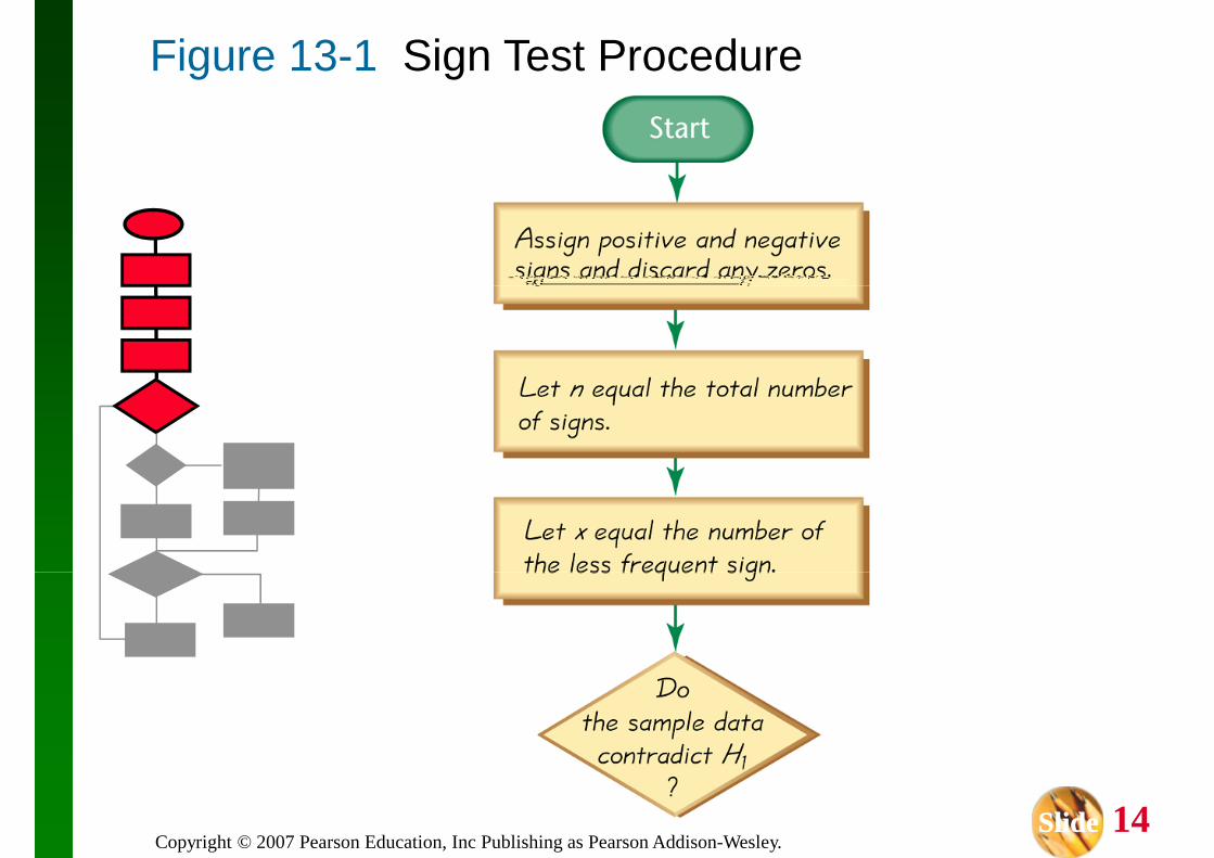
The sign test is a nonparametric (distribution The sign test is a nonparametric (distribution free) test that uses plus and minus signs to test different claims, including:
For n ≤≤≤≤ 25, critical x values are in Table A -7.
For n > 25, critical z values are in Table A -2.
Claims Involving Matched Pairs
When using the sign test with data that are matched pairs, we convert the raw data to plus and minus signs as follows: plus and minus signs as follows:
1. Subtract each value of the second variable from the corresponding value of the first variable.
Use the data in Table 13-3 with a 0.05 significance level to test the claim that there is no difference betwe en the yields from the regular and kiln -dried seed. yields from the regular and kiln -dried seed.
Use the data in Table 13-3 with a 0.05 significance level to test the claim that there is no difference betwe en the yields from the regular and kiln -dried seed.
H0: The median of the differences is equal to 0.
H1: The median of the differences is not equal to 0.
x = minimum(7, 4) = 4 (From Table 13-3, there are 7 negative signs and 4 positive signs.)
Critical value = 1 (From Table A -7 where n = 11 and αααα = 0.05)
Example: Yields of Corn from Different Seeds
Use the data in Table 13-3 with a 0.05 significance level to test the claim that there is no difference betwe en the yields from the regular and kiln -dried seed.
H0: The median of the differences is equal to 0.
H1: The median of the differences is not equal to 0.
With a test statistic of x = 4 and a critical value of 1, we fail to reject the null hypothesis of no differe nce.
we fail to reject the null hypothesis of no differe nce.
There is not sufficient evidence to warrant rejecti on of the claim that the median of the differences is equal to 0.
Claims Involving Nominal Data
The nature of nominal data limits the The nature of nominal data limits the calculations that are possible, but we can identify the proportion of the sample data
Then we can test claims about the corresponding population proportion p.
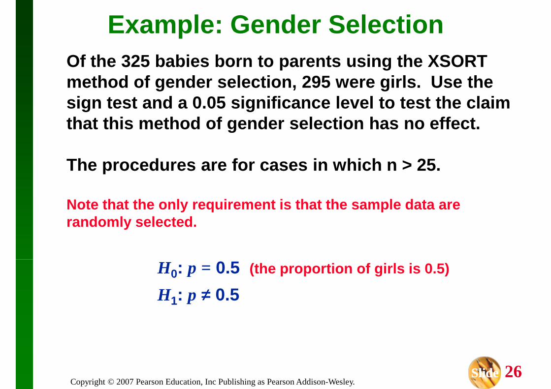
Example: Gender SelectionOf the 325 babies born to parents using the XSORT method of gender selection, 295 were girls. Use th e sign test and a 0.05 significance level to test the claim that this method of gender selection has no effect.that this method of gender selection has no effect.
The procedures are for cases in which n > 25.
Note that the only requirement is that the sample d ata are randomly selected.
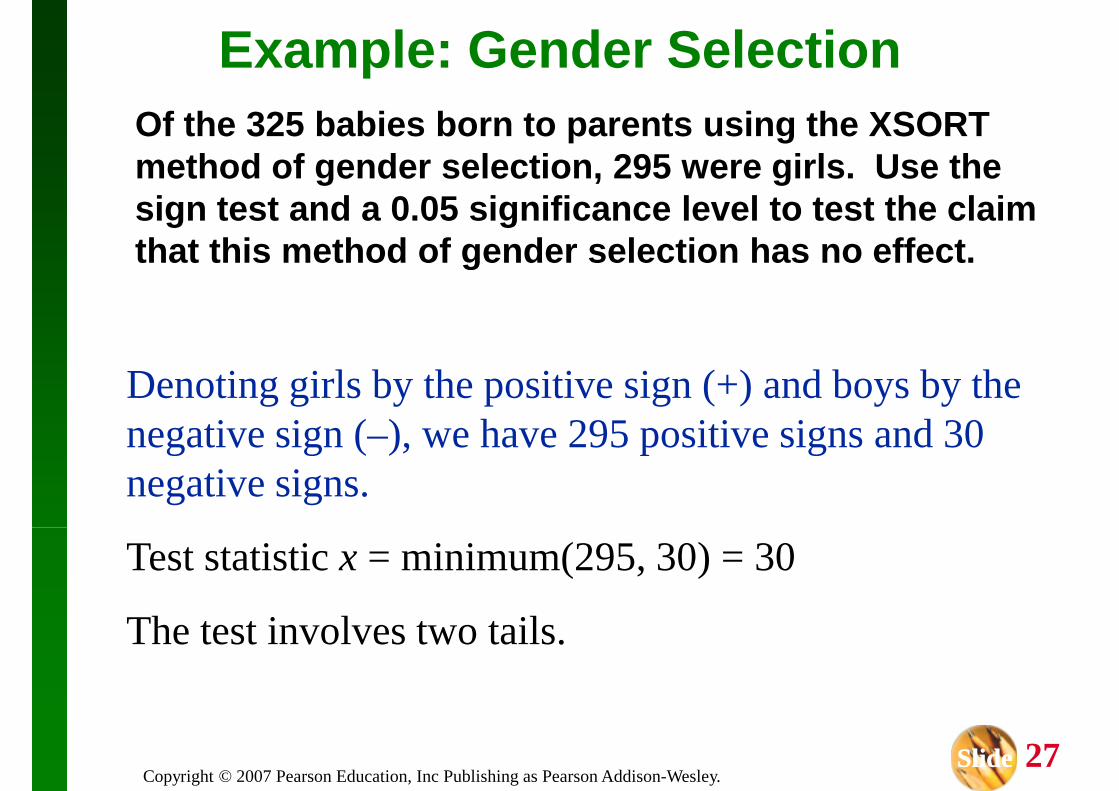
Example: Gender SelectionOf the 325 babies born to parents using the XSORT method of gender selection, 295 were girls. Use th e sign test and a 0.05 significance level to test the claim that this method of gender selection has no effect.that this method of gender selection has no effect.
Denoting girls by the positive sign (+) and boys by the negative sign (–), we have 295 positive signs and 30 negative signs.
Example: Gender SelectionOf the 325 babies born to parents using the XSORT method of gender selection, 295 were girls. Use th e sign test and a 0.05 significance level to test the claim that this method of gender selection has no effect.that this method of gender selection has no effect.
Example: Gender SelectionOf the 325 babies born to parents using the XSORT method of gender selection, 295 were girls. Use th e sign test and a 0.05 significance level to test the claim that this method of gender selection has no effect.that this method of gender selection has no effect.
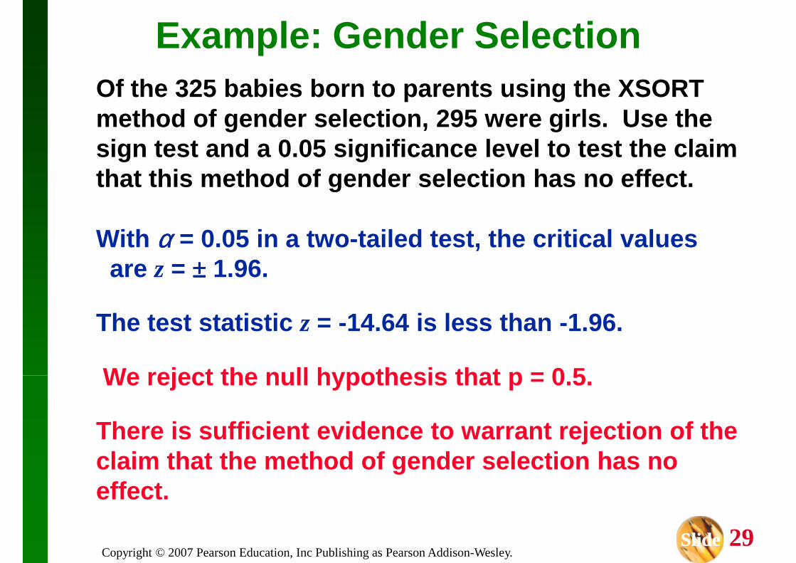
With αααα = 0.05 in a two-tailed test, the critical values are z = ±±±± 1.96.
There is sufficient evidence to warrant rejection o f the claim that the method of gender selection has no effect.
Example: Gender SelectionOf the 325 babies born to parents using the XSORT method of gender selection, 295 were girls. Use th e sign test and a 0.05 significance level to test the claim that this method of gender selection has no effect.that this method of gender selection has no effect.
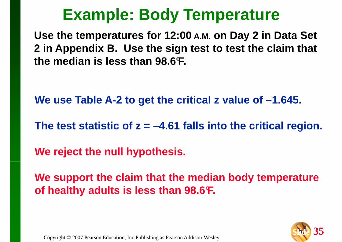
Example: Body TemperatureUse the temperatures for 12:00 A.M. on Day 2 in Data Set 2 in Appendix B. Use the sign test to test the cla im that the median is less than 98.6°F.
There are 68 subjects with temperatures below 98.6° F, 23 subjects with temperatures above 98.6°F, and 15 subjects with temperatures equal to 98.6°F.
Since the claim is that the median is less than 98.6°F. the test involves only the left tail.
Example: Body TemperatureUse the temperatures for 12:00 A.M. on Day 2 in Data Set 2 in Appendix B. Use the sign test to test the cla im that the median is less than 98.6°F.
Discard the 15 zeros.
Use ( – ) to denote the 68 temperatures below 98.6° F, and use ( + ) to denote the 23 temperatures above 98.6°F.
Example: Body TemperatureUse the temperatures for 12:00 A.M. on Day 2 in Data Set 2 in Appendix B. Use the sign test to test the cla im that the median is less than 98.6°F.
Example: Body TemperatureUse the temperatures for 12:00 A.M. on Day 2 in Data Set 2 in Appendix B. Use the sign test to test the cla im that the median is less than 98.6°F.
We use Table A -2 to get the critical z value of –1.645.
The test statistic of z = –4.61 falls into the critical region.
We support the claim that the median body temperatu re of healthy adults is less than 98.6°F.
Example: Body TemperatureUse the temperatures for 12:00 A.M. on Day 2 in Data Set 2 in Appendix B. Use the sign test to test the cla im that the median is less than 98.6°F.
Sign tests where data are assigned plus or minus signs and then tested to see if the number of plus signs and then tested to see if the number of plus and minus signs is equal.
H1: The matched pairs have differences that come from a population with a nonzero median.
1. The data consist of matched pairs that have
Wilcoxon Signed-Ranks TestRequirements
1. The data consist of matched pairs that have been randomly selected.
2. The population of differences (found from the pairs of data) has a distribution that is approximately symmetric, meaning that the left half of its histogram is roughly a mirror image of
For n > 30, the critical z values are found in Table A -2.
Procedure for Finding the Value of the Test Statistic
Step 1: For each pair of data, find the difference d by subtracting the second value from the first. Keep the signs, but d iscard any
pairs for which d = 0.pairs for which d = 0.
Step 2: Ignore the signs of the differences , then sort the differences from lowest to highest and replace the differences by the corresponding rank value. When differences have th e same numerical value, assign to them the mean of the ran ks involved in the tie.
Step 3: Attach to each rank the sign difference fr om which it came.
Step 8: When forming the conclusion, reject the nu ll hypothesis if the sample data lead to a test statistic that is in the critical region - that is, the test statistic is less than or equal to the critical value(s). Otherwise, fail to reject the nu ll hypothesis.
Example: Does the Type of SeedAffect Corn Growth?
Use the data in Table 13-4 with the Wilcoxon signed -ranks test and 0.05 significance level to test the claim that there is no difference between the yields from the regula r and is no difference between the yields from the regula r and kiln-dried seed.
Use the data in Table 13-4 with the Wilcoxon signed -ranks test and 0.05 significance level to test the claim that there is no difference between the yields from the regula r and
Example: Does the Type of SeedAffect Corn Growth?
is no difference between the yields from the regula r and kiln-dried seed.
H0: There is no difference between the times of the first and second trials.
Step 3: The bottom row of Table 13 -4 is created by attaching to each rank the sign of the corresponding differences.
Example: Does the Type of SeedAffect Corn Growth?
Step 3 (cont.): If there really is no difference Step 3 (cont.):
Calculate the Test Statistic
Step 3 (cont.): If there really is no difference between the yields from the two types of seed (as in the null hypothesis), we expect the sum of the positive ranks to be approximately equal to the sum of the absolute values of the negative ranks.
Step 6: Letting n be the number of pairs of data for which the difference d is not 0, we have n = 11.
Example: Does the Type of SeedAffect Corn Growth?
Step 7: Because n = 11, we have n ≤ 30, so we Step 7:
Calculate the Test Statistic
Step 7: Because n = 11, we have n ≤ 30, so we use a test statistic of T = 15. From Table A -8, the critical T = 11 (using n = 11 and αααα = 0.05 in two tails).
Step 8: The test statistic T = 15 is not less than or equal to the critical value of 11, so we fail to
samples that are not related or somehow matched or paired.
Definition
The Wilcoxon rank -sum test is a nonparametric test that uses ranks of sample data from two independent populations. It is used to test the independent populations. It is used to test the null hypothesis that the two independent samples come from populations with equal medians.
H0: The two samples come from populations with equal medians.
H1: The two samples come from populations with different medians.
Basic Concept
If two samples are drawn from If two samples are drawn from identical populations and the individual values are all ranked as one combined collection of values, then the high and low ranks should fall evenly between the two samples.
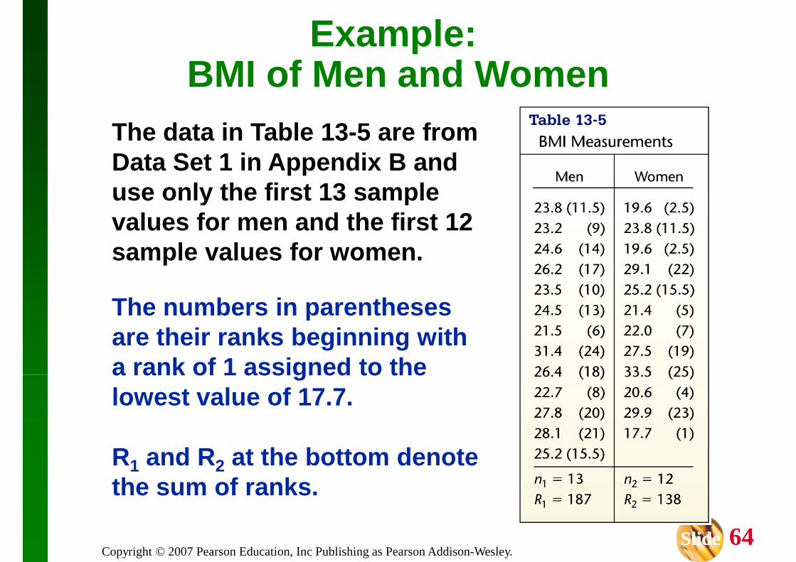
Use the data in Table 13-5 with the Wilcoxon rank-s um test and a 0.05 significance level to test the clai m that the median BMI of men is equal to the median BMI of the median BMI of men is equal to the median BMI of women.
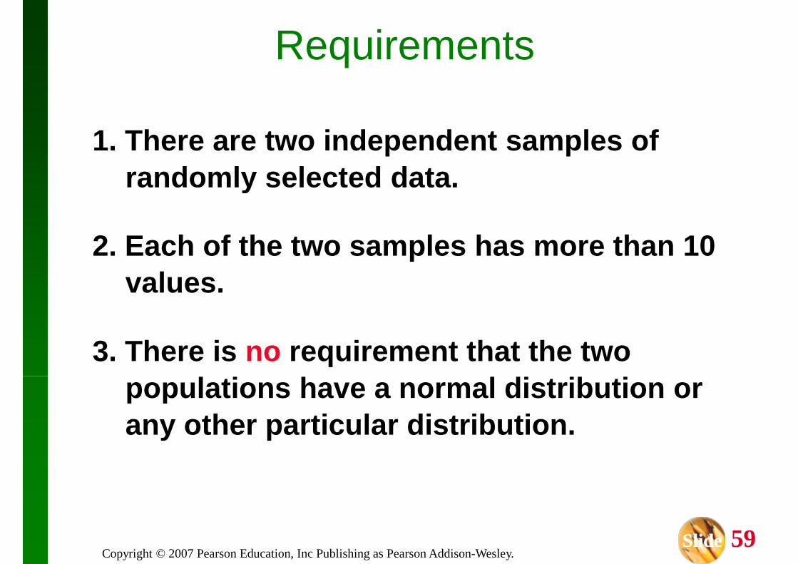
The requirements of having two independent and random samples and each having more than 10 values are met.
H0: Men and women have BMI values with equal medians
H1: Men and women have BMI values with medians that are not equal
Use the data in Table 13-5 with the Wilcoxon rank-s um test and a 0.05 significance level to test the clai m that the median BMI of men is equal to the median BMI of
Example: BMI of Men and Women
the median BMI of men is equal to the median BMI of women.
Procedures .
1. Rank all 25 BMI measurements combined. This is done in Table 13 -5.
Use the data in Table 13-5 with the Wilcoxon rank-s um test and a 0.05 significance level to test the clai m that the median BMI of men is equal to the median BMI of the median BMI of men is equal to the median BMI of women.
A large positive value of z would indicate that the higher ranks are found disproportionately in Sample 1, and a large negative value of z would
Sample 1, and a large negative value of z would indicate that Sample 1 had a disproportionate share of lower ranks.
Example: BMI of Men and Women
Use the data in Table 13-5 with the Wilcoxon rank-s um test and a 0.05 significance level to test the clai m that the median BMI of men is equal to the median BMI of the median BMI of men is equal to the median BMI of women.
We have a two tailed test (with αααα = 0.05), so thecritical values are 1.96 and –1.96.
The test statistic of 0.98 does not fall within the critical region, so we fail to reject the null hypo thesis
critical region, so we fail to reject the null hypo thesis that men and women have BMI values with equal medians.
It appears that BMI values of men and women are basically the same.
The preceding example used only 13 of the 40
Example: BMI of Men and Women
The preceding example used only 13 of the 40 sample BMI values for men listed in Data Set 1 in Appendix B, and it used only 12 of the 40 BMI values for women. Do the results change if we use all 40 sample values for both men and women?
Created by Erin Hodgess, Houston, TexasRevised to accompany 10th Edition, Jim Zimmer, Chattanooga State,
Chattanooga, TN
Key Concept
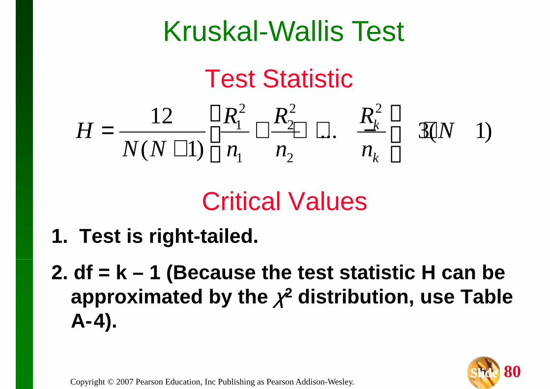
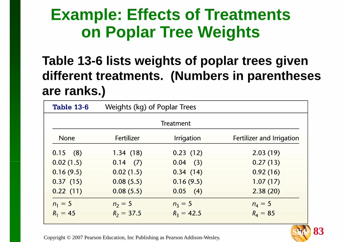
This section introduces the Kruskal -This section introduces the Kruskal -Wallis test, which uses ranks of data from three or more independent samples to test the null hypothesis that the samples come from populations with equal medians.
Created by Erin Hodgess, Houston, TexasRevised to accompany 10th Edition, Jim Zimmer, Chattanooga State,
Chattanooga, TN
Key Concept
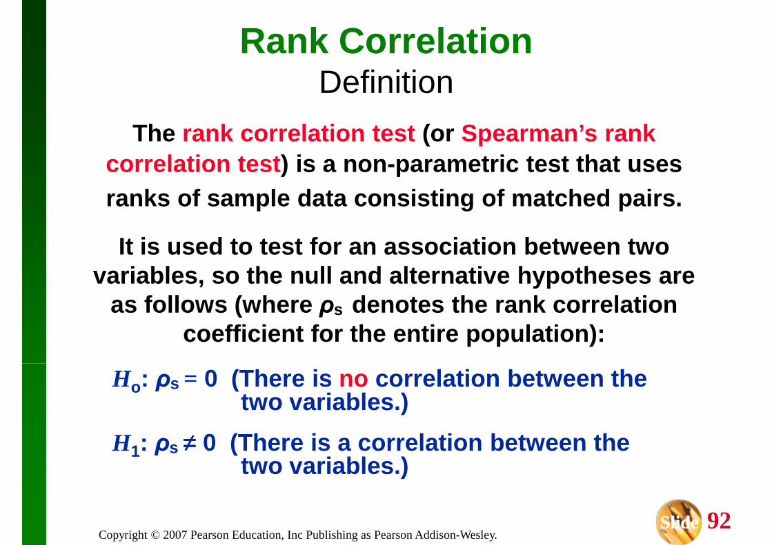
This section describes the nonparametric method of rank correlation, which uses paired data to test for an association between two data to test for an association between two variables.
In Chapter 10 we used paired sample data to compute values for the linear correlation coefficient r, but in this section we use ranks as
Ho: ρs = 0 (There is no correlation between the two variables.)
H1: ρs ≠≠≠≠ 0 (There is a correlation between the two variables.)
AdvantagesRank correlation has these advantages over the parametric methods discussed
in Chapter 10:
1. The nonparametric method of rank correlation can be used in a wider variety of circumstances than the parametric method of linear correlation. With rank correlation, we can analyze paired data that are ranks or can
2. Rank correlation can be used to detect some (not all) relationships that are not linear.
Disadvantages
A disadvantage of rank correlation is its efficiency rating of 0.91, as described in Section 13 -1.Section 13 -1.
This efficiency rating shows that with all other circumstances being equal, the nonparametric approach of rank correlation requires 100 pairs of sample data to achieve the same results as only 91 pairs of sample observations
as only 91 pairs of sample observations analyzed through parametric methods, assuming that the stricter requirements of the parametric approach are met.
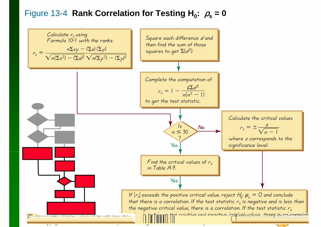
Figure 13-4 Rank Correlation for Testing H0: ρρρρs = 0
1. The sample paired data have been randomly selected. randomly selected.
2. Unlike the parametric methods of Section 10 -2, there is no requirement that the sample pairs of data have a bivariate normal distribution. There is no requirement of a normal distribution for any population.
No ties:After converting the data in each sample to ranks, if there are no ties among ranks for either variable, the exact value of the test statistic can be calculated using this formula:
Ties:After converting the data in each sample to ranks, if either variable has ties among its ranks, the exact value of the test statistic rs can be found by using Formula 10-1 with the
1n −where the value of z corresponds to the significance
level. (For example, if αααα = 0.05, z – 1.96.)
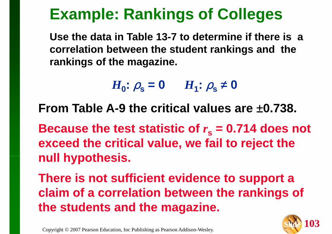
Example: Rankings of CollegesUse the data in Table 13-7 to determine if there is a correlation between the student rankings and the rankings of the magazine.
Example: Rankings of CollegesUse the data in Table 13-7 to determine if there is a correlation between the student rankings and the rankings of the magazine.
Example: Rankings of CollegesUse the data in Table 13-7 to determine if there is a correlation between the student rankings and the rankings of the magazine.
H : ρρρρ = 0 H : ρρρρ ≠≠≠≠ 0H0: ρρρρs = 0 H1: ρρρρs ≠≠≠≠ 0
From Table A -9 the critical values are ±±±±0.738.
Because the test statistic of rs = 0.714 does not exceed the critical value, we fail to reject the null hypothesis.
There is not sufficient evidence to support a claim of a correlation between the rankings of the students and the magazine.
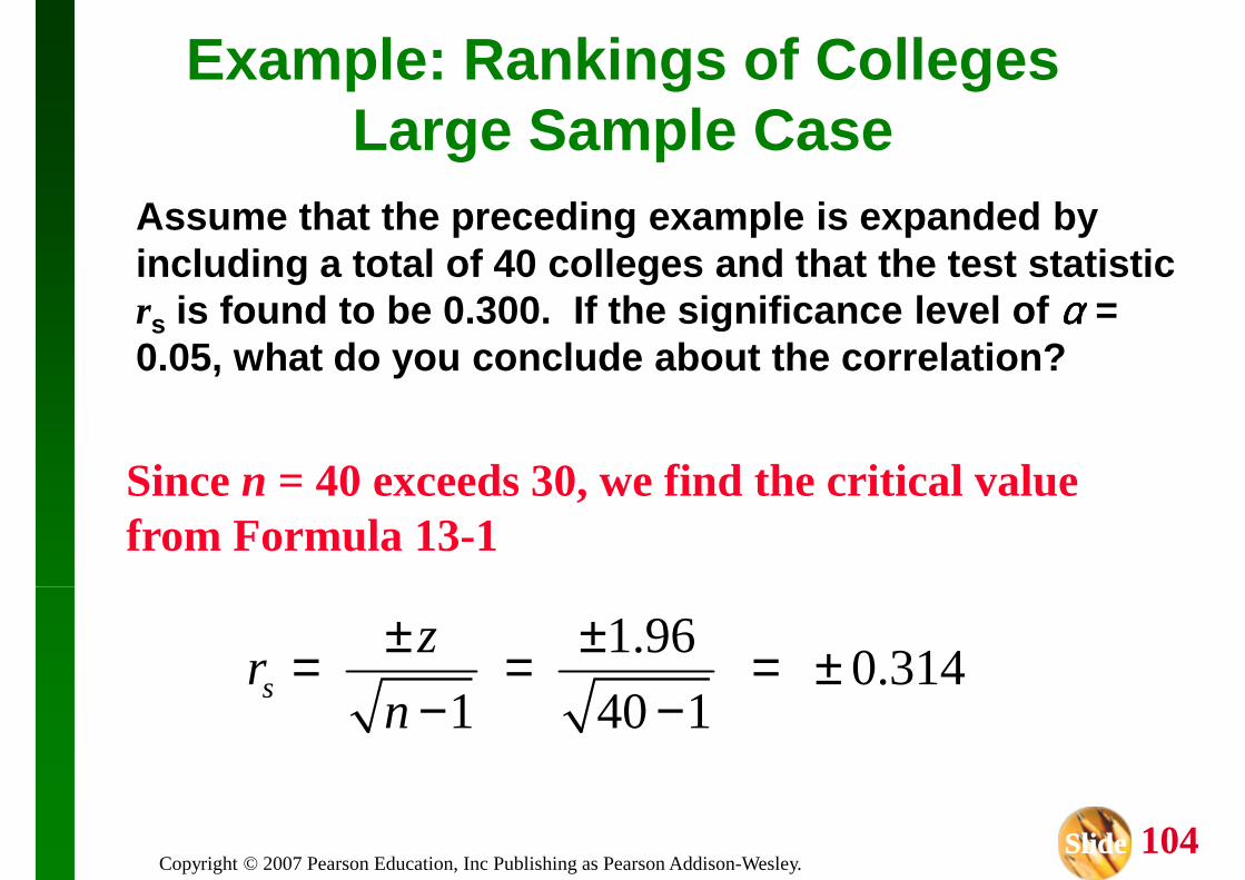
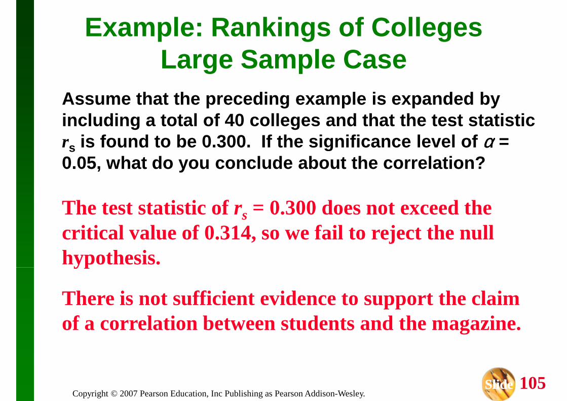
Assume that the preceding example is expanded by including a total of 40 colleges and that the test statistic r is found to be 0.300. If the significance level of αααα =
Example: Rankings of CollegesLarge Sample Case
rs is found to be 0.300. If the significance level of αααα = 0.05, what do you conclude about the correlation?
Since n = 40 exceeds 30, we find the critical value from Formula 13-1
Assume that the preceding example is expanded by including a total of 40 colleges and that the test statistic r is found to be 0.300. If the significance level of αααα =
Example: Rankings of CollegesLarge Sample Case
rs is found to be 0.300. If the significance level of αααα = 0.05, what do you conclude about the correlation?
The test statistic of rs = 0.300 does not exceed the critical value of 0.314, so we fail to reject the null hypothesis.
There appears to be correlation between the number of games played and the score.
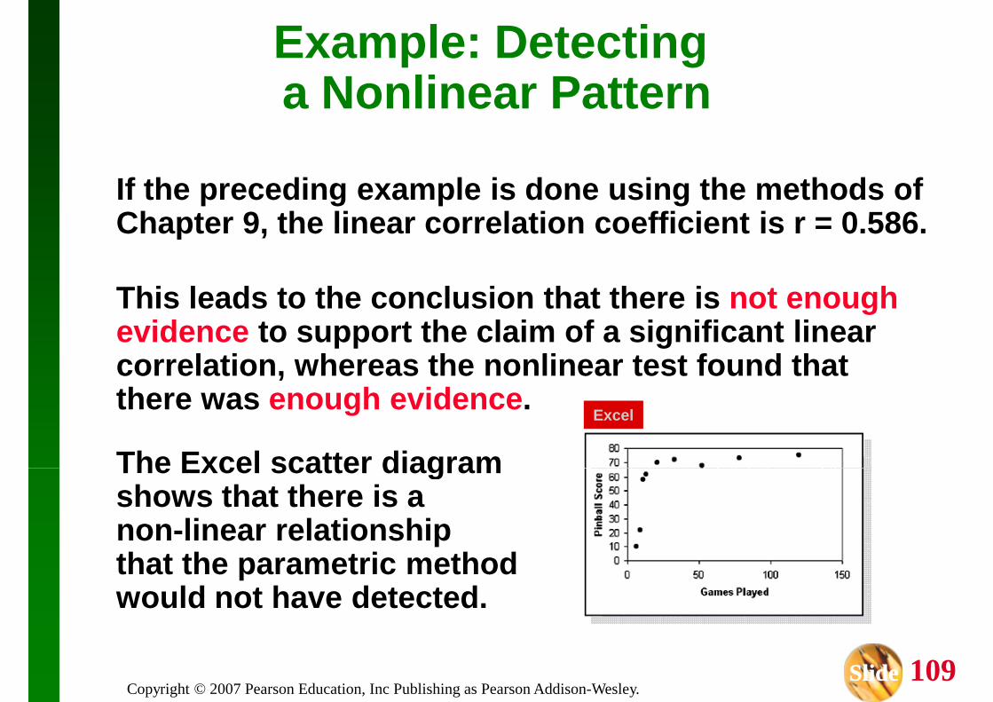
Example: Detecting a Nonlinear Pattern
If the preceding example is done using the methods of Chapter 9, the linear correlation coefficient is r = 0.586.Chapter 9, the linear correlation coefficient is r = 0.586.
This leads to the conclusion that there is not enough evidence to support the claim of a significant linear correlation, whereas the nonlinear test found that there was enough evidence .
Created by Erin Hodgess, Houston, TexasRevised to accompany 10th Edition, Jim Zimmer, Chattanooga State,
Chattanooga, TN
Key Concept
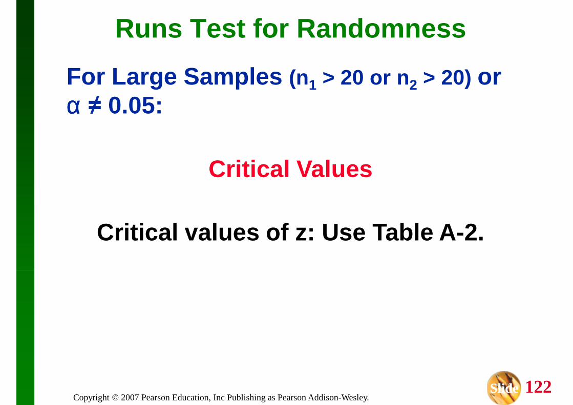
This section introduces the runs test for randomness, which can be used to determine whether the sample data in a sequence are in a whether the sample data in a sequence are in a random order.
This test is based on sample data that have two characteristics, and it analyzes runs of those characteristics to determine whether the runs appear to result from some random process, or
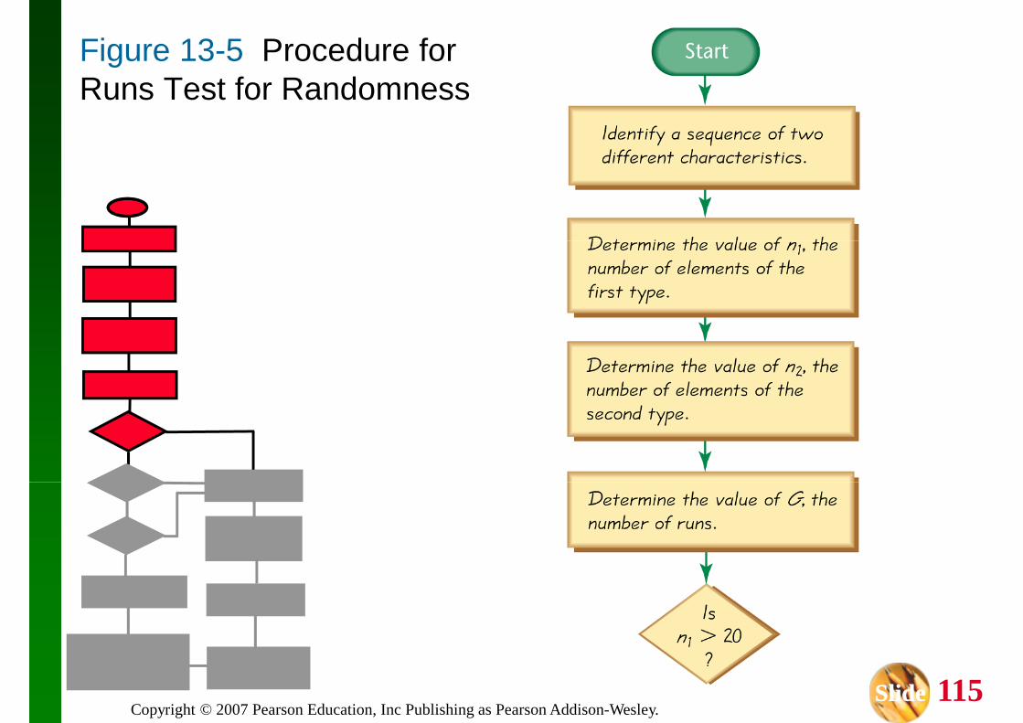
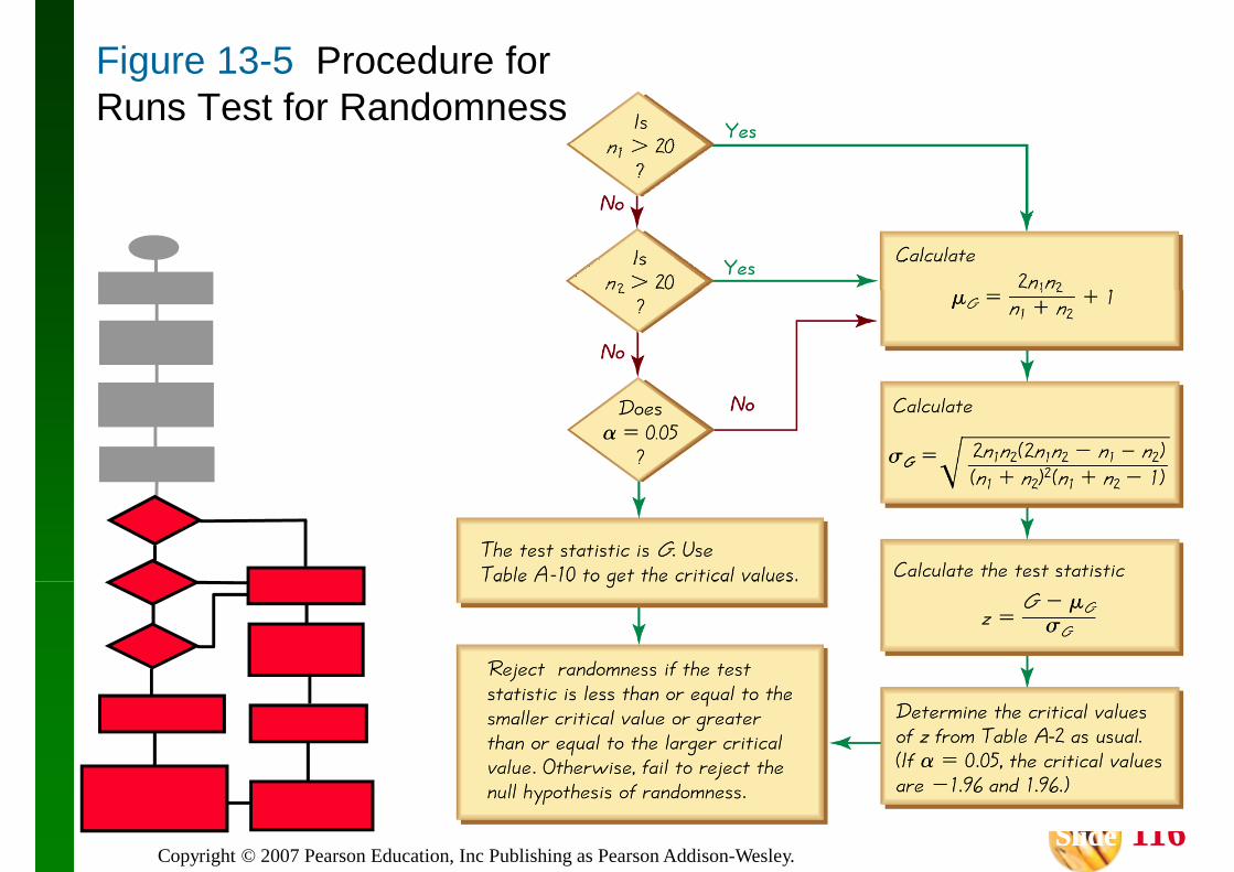
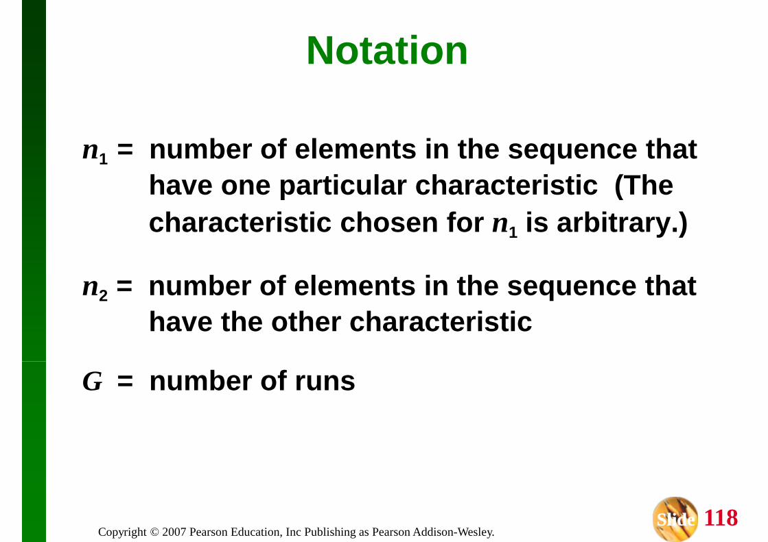
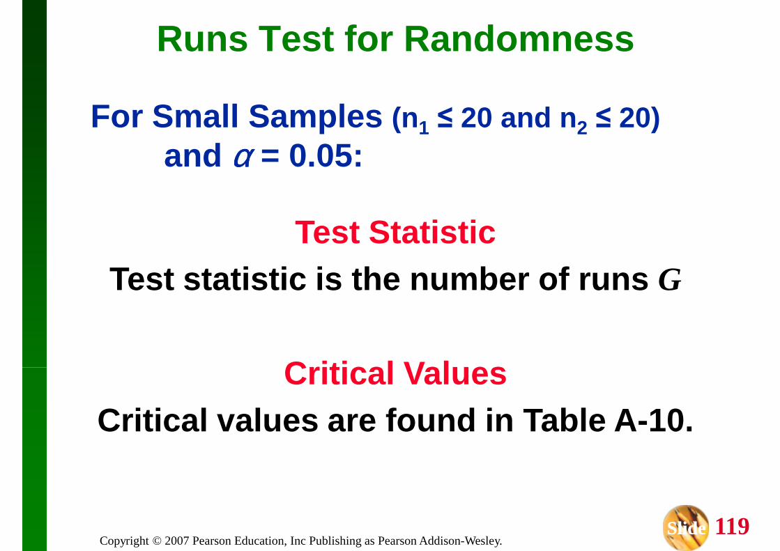
The runs test uses the number of runs in a sequence of sample data to test for randomness in the order of the data.
Fundamental Principles of the Run Test
Reject randomness if the number of runs is very low or very high.Example: The sequence of genders FFFFFMMMMM is Example: The sequence of genders FFFFFMMMMM is not random because it has only 2 runs, so the numbe r of runs is very low .
Example: The sequence of genders FMFMFMFMFM is not random because there are 10 runs, which is very high .
1. The sample data are arranged according to some ordering scheme, such as the order some ordering scheme, such as the order in which the sample values were obtained.
2. Each data value can be categorized into one of two separate categories (such as male/female).
n1 = number of elements in the sequence that have one particular characteristic (The have one particular characteristic (The characteristic chosen for n1 is arbitrary.)
n2 = number of elements in the sequence that have the other characteristic
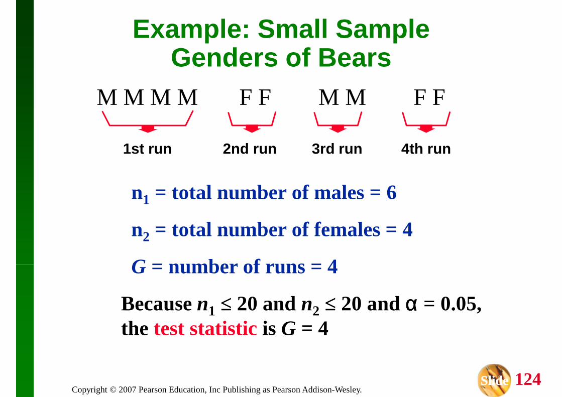
Listed below are the genders of the first 10 bears from Data Set 6 in Appendix B. Use a 0.05 significance level to test for randomness in the sequence of genders.to test for randomness in the sequence of genders.
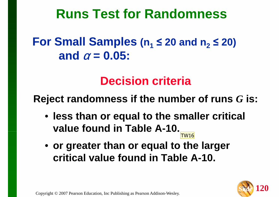
it greater than or equal to 9, we do not reject randomness.
It appears the sequence of genders is random.
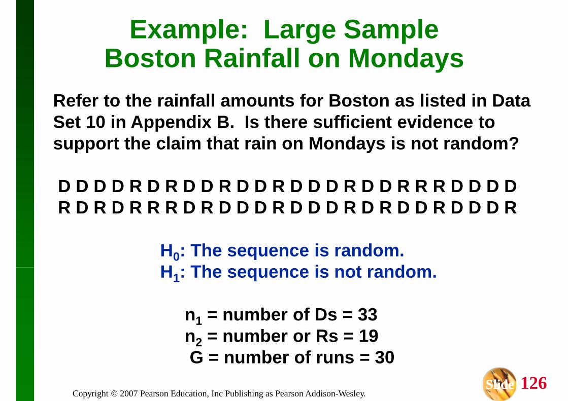
Refer to the rainfall amounts for Boston as listed in Data Set 10 in Appendix B. Is there sufficient evidence to support the claim that rain on Mondays is not rando m?
Example: Large SampleBoston Rainfall on Mondays
support the claim that rain on Mondays is not rando m?
D D D D R D R D D R D D R D D D R D D R R R D D D D R D R D R R R D R D D D R D D D R D R D D R D D D R
H0: The sequence is random.H : The sequence is not random.