Introduction to information theory and coding

Louis WEHENKEL

Set of slides No 6

Overview of (irreversible) image compression

• Motivations

• Image representations

• Sources of redundancy

• Image compression systems

• Brief introduction to wavelets

IT 2000-6, slide 1

Motivations for image compression (and to some extent for sound compression)

Avantage of digital image representations : immunity to noise

Disadvantages : huge volumes of data if not compressed

Examples

A high resolution image= some MB.

A video sequence :≈ 20 images/s : 1minute≈ 1GB.

Present day image compression techniques

⇒ compression rates→ 100.

⇒ makes possible what would be impossible otherwise.

⇒ image processing : one of the most used techniques in many fields (more and more).

⇒ Multimedia DB, medical applications, legal, digital archives...

IT 2000-6, slide 2

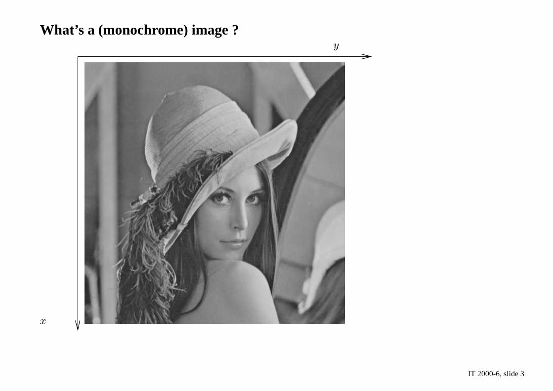
What’s a (monochrome) image ?

x

y

IT 2000-6, slide 3

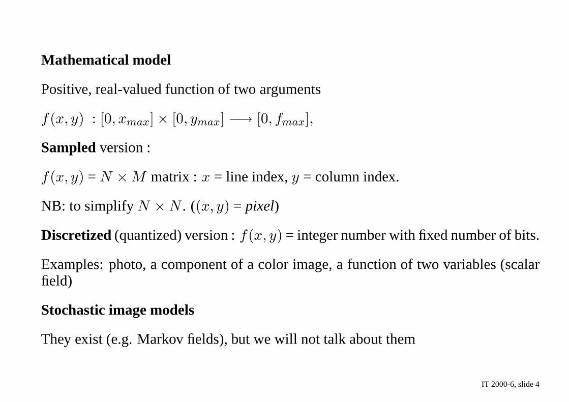
Mathematical model

Positive, real-valued function of two arguments

f(x, y) : [0, xmax] × [0, ymax] −→ [0, fmax],

Sampled version :

f(x, y) = N × M matrix : x = line index,y = column index.

NB: to simplify N × N . ((x, y) = pixel)

Discretized (quantized) version :f(x, y) = integer number with fixed number of bits.

Examples: photo, a component of a color image, a function of two variables (scalarfield)

Stochastic image models

They exist (e.g. Markov fields), but we will not talk about them

IT 2000-6, slide 4

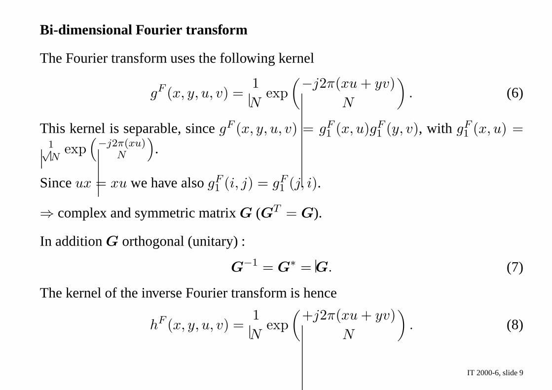
Image transforms

NB: generalization of the Fourier transform

Goal: represent image in a way well suited for a class of operations.

E.g.: Fourier transform “makes easy” linear operations (convolution).

Here: goal= facilitate data compression (reversible or irreversible).

Reminder (in the temporal domain = unidimensional, sampled)

t(w) =N−1∑

t=0

f(t)g(t, w)

g(t, w) = kernel (family ofN basis functions indexed byw)

Inverse transform (when it exists)f(t) =∑N−1

w=0 t(w)h(t, w).

IT 2000-6, slide 5

Vector representation :

g(t, w) = N × N matrix,f(t) andt(w) line vectors.

⇒ transformation = matrix product

t = fG, f = tH ⇒ H = G−1

Orthogonal Bases : orthogonal matricesG−1 = GT .

In the complex case :G−1 = G∗.

⇒ transformation = change of basis

NB: continuous case∑N−1

0 →∫ T0 ...

Anyway : transformation =linear operation⇒ transform of linear combination = linear combination of transforms.

Physical interpretation :

t(w) measures similarity off(t) andg(t, w) (analog to dictionary match)

IT 2000-6, slide 6

Generalization to images

The transformG of an imagef(x, y) (dimensionsN × N ) usingkernel g(·, ·, ·, ·) isthe new imageN × N

G(f) = T (u, v) =N−1∑

x=0

N−1∑

y=0

f(x, y)g(x, y, u, v). (1)

The transform is non-singular, and has an inverse transformH which kernel ish(·, ·, ·, ·),if ∀f(x, y)

f(x, y) = H(G(f)) = H(T ) =N−1∑

u=0

N−1∑

v=0

T (u, v)h(x, y, u, v). (2)

The functionsg(i, j, ·, ·) and h(·, ·, i, j) may be interpreted as a set ofN2 “basisfunctions” in a series expansion.

IT 2000-6, slide 7

Construction of image transforms

Kernelg(·, ·, ·, ·) is separable ifg(x, y, u, v) = g1(x, u)g2(y, v).It is said to be symmetric if we can takeg1(·, ·) = g2(·, ·). (Same forh)

⇒ Multi-dimensional transforms are obtained by successive applications of unidi-mensional ones.

One first transforms theN lines, then theN columns of the result :T = GT FG.

T (u, v) =N−1∑

x=0

N−1∑

y=0

f(x, y)g(x, y, u, v) (3)

=N−1∑

x=0

N−1∑

y=0

f(x, y)g1(x, u)g1(y, v) (4)

=N−1∑

x=0

g1(x, u)

N−1∑

y=0

f(x, y)g1(y, v)

(5)

henceT = GT [FG] = GT FG. (Invertible iff Gis non-singular)

IT 2000-6, slide 8

Bi-dimensional Fourier transform

The Fourier transform uses the following kernel

gF (x, y, u, v) =1

Nexp

(−j2π(xu + yv)

N

)

. (6)

This kernel is separable, sincegF (x, y, u, v) = gF1 (x, u)gF

1 (y, v), with gF1 (x, u) =

1√N

exp(

−j2π(xu)N

)

.

Sinceux = xu we have alsogF1 (i, j) = gF

1 (j, i).

⇒ complex and symmetric matrixG (GT = G).

In additionG orthogonal (unitary) :

G−1 = G∗ = G. (7)

The kernel of the inverse Fourier transform is hence

hF (x, y, u, v) =1

Nexp

(

+j2π(xu + yv)

N

)

. (8)

IT 2000-6, slide 9

Comments

Technique may be extended to more than 2 dimensions.

FFT algorithm may be used (⇒ O(N × N log N) operations) : quasi-linear.

Sampling theorem : applies also. (choice of sampling intervals as a function of thefrequency spectrum of the image)

Applications : signal processing...

Other transforms : Walsh and Hadamard

“Discrete Versions” of the Fourier transform.

Applicable ifN = 2n.

Values of the basis functions :± 1√N

.

⇒ calculations simpler, physical interpretation similar.

IT 2000-6, slide 10

Kernel of the Walsh (left) and Hadamard (right) transforms (N = 8)

u

x 0 1 2 3 4 5 6 70 + + + + + + + +1 + + + + - - - -2 + + - - + + - -3 + + - - - - + +4 + - + - + - + -5 + - + - - + - +6 + - - + + - - +7 + - - + - + + -

u

x 0 1 2 3 4 5 6 70 + + + + + + + +1 + - + - + - + -2 + + - - + + - -3 + - - + + - - +4 + + + + - - - -5 + - + - - + - +6 + + - - - - + +7 + - - + - + + -

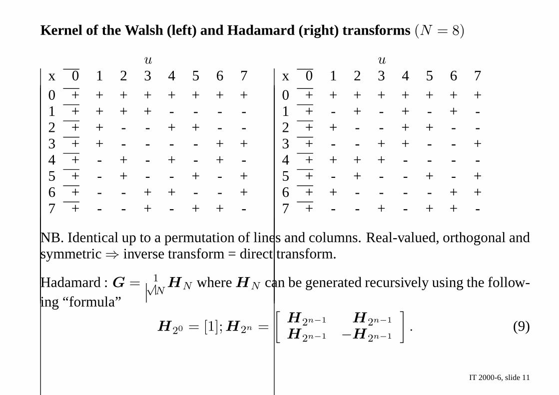
NB. Identical up to a permutation of lines and columns. Real-valued, orthogonal andsymmetric⇒ inverse transform = direct transform.

Hadamard :G = 1√N

HN whereHN can be generated recursively using the follow-ing “formula”

H20 = [1]; H2n =

[

H2n−1 H2n−1

H2n−1 −H2n−1

]

. (9)

IT 2000-6, slide 11

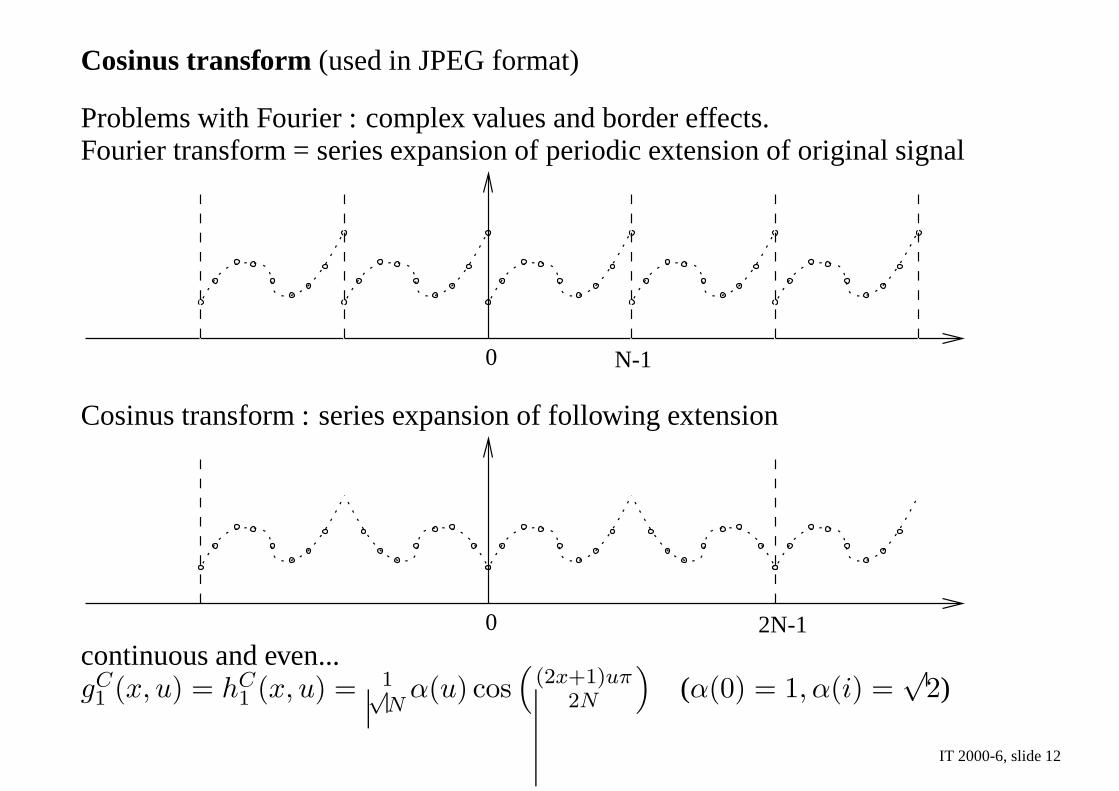
Cosinus transform (used in JPEG format)

Problems with Fourier : complex values and border effects.Fourier transform = series expansion of periodic extensionof original signal

N-10

Cosinus transform : series expansion of following extension

2N-10

continuous and even...gC1 (x, u) = hC

1 (x, u) = 1√N

α(u) cos(

(2x+1)uπ

2N

)

(α(0) = 1, α(i) =√

2)

IT 2000-6, slide 12

Cosinus transform of Lena

Cosinus transform quantized at level 100.0Entropy = 0.2493 (zero order, per pixel) Compression ratio : 32 (w.r.t. original image)

Decoded version of image

IT 2000-6, slide 13

Cosinus transform of Lena

Cosinus transform quantized at level 20.0Entropy = 1.4689 (zero order, per pixel) Compression ratio : 5.4 (w.r.t. original image)

Decoded version of image

IT 2000-6, slide 14

Operations which are easy on the transformed images

Filtering : e.g. HF noise vs LF signal.

Zooming, smoothing.

From the viewpoint of information theory

Concentration of entropy in a reduced number of pixels⇒ image compression.

Data transmission in an appropriate order :

⇒ first send main information, then details

IT 2000-6, slide 15

Sources of redundancy

(Remark : terminology used in image processing literature.)

1. Coding redundancy. Factor2 − 3

Some grey-levels are more frequent then others (cf. histogram)

2. Inter-pixel redundancy. Factor> 10

Nearby pixels are similar (continuity of the bi-dimensional signal)

⇒ HF components are normally of low intensity.

3. Psycho-visual redundancy. Factor> 100

Our biological vision system is unable to detect all the details and is (hence) “robust”with respect to certain types of approximations.

⇒ allows to use irreversible compression techniques withoutimpact on perception.

IT 2000-6, slide 16

Image compression systems

Canal

Canal

(a) Image Encoder

(b) Image Decoder

f(x, y)T T̂

T̂f̂(x, y)

Quantization

Decoding

Transform Source Coding

Inverse transform

NB: the central part of the encoder is not necessarily present.

First block: change representation to reduce inter-pixel redundancy and facilitatequantization (take advantage of phsycho-visual redundancy).

Last block: see data compression techniques.

IT 2000-6, slide 17

Some approaches

A. Reversible

“Zero order”

In the binary case : coding of black and white areas (cf. FAX)

Differential coding : one transforms the image and codes thedifferences.

Bit planes.

Predictive coding :

One uses a predictive model to estimate the value offn given already seen pixels andone encodes only the prediction errors of this model.

NB: Differential coding = “naive” version of predictive coding.

One can use highly sophisticated prediction models (neuralnetworks...) :⇒ compromize between model complexity vs entropy of prediction errors⇒ General principle in automatic learning (Minimum Description Length).

IT 2000-6, slide 18

B. Irreversible

Predictive coding

We don’t encode prediction errors (or very roughly)

Use of image transforms

Often applied locally.

One doesn’t encode HF content (or very roughly).

C. Standards

Binary images : “run-length” encoding for FAX.

Monochrome images : JPEG (cosinus transform8 × 8 plus Huffman.)

Sequences of color images : MPEG (cosinus transform, plus predictive models alongtime axis).

IT 2000-6, slide 19

A short introduction to wavelets

Problem : basis functions of most classical transforms are not very good to representimages compactly.

Reasons : “non-stationary” aspect⇒ frequency content depends on spatial coordi-nates.

⇒ requires the use of image transforms on small windows of the original image (cf.JPEG).

Wavelets: constructive approach to build a catalog (dictionary) of well suited signals.

Main idea : extract frequency componentslocalized in space (or time)

The higher the frequency, the more local the information extracted.

Example : Haar wavelets (local version of Walsh-Hadamard)

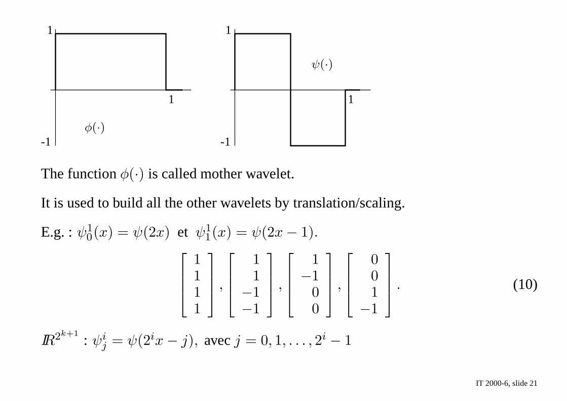
IT 2000-6, slide 20

1

1

-1

1

1

-1φ(·)

ψ(·)

The functionφ(·) is called mother wavelet.

It is used to build all the other wavelets by translation/scaling.

E.g. :ψ10(x) = ψ(2x) et ψ1

1(x) = ψ(2x− 1).

1111

,

11

−1−1

,

1−1

00

,

001

−1

. (10)

IR2k+1

: ψij = ψ(2ix− j), avecj = 0, 1, . . . , 2i − 1

IT 2000-6, slide 21

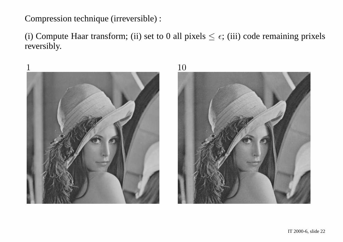
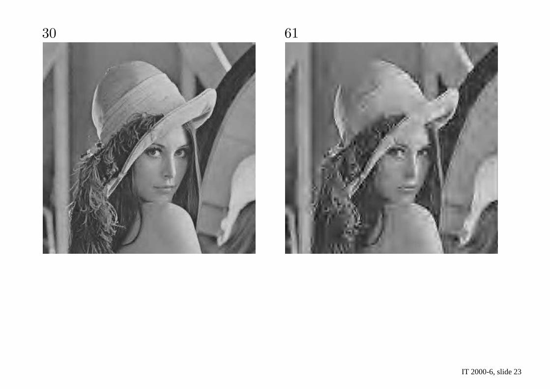
Compression technique (irreversible) :

(i) Compute Haar transform; (ii) set to 0 all pixels≤ ǫ; (iii) code remaining prixelsreversibly.

1 10

IT 2000-6, slide 22

30 61

IT 2000-6, slide 23