Page 1
Development of Solvent Selection Criteria Based on Diffusion Rate, Mixing Quality, and
Solvent Retrieval for Optimal Heavy-Oil and Bitumen Recovery at Different Temperatures
by
Andrea Paola Marciales Ramirez
A thesis submitted in partial fulfillment of the requirements for the degree of
Master of Science
in
Petroleum Engineering
Department of Civil and Environmental Engineering
University of Alberta
© Andrea Paola Marciales Ramirez, 2015
Page 2
ii
Abstract
Heavy-oil and bitumen recovery requires high recovery factors to offset the extreme high
cost of the process. Attention has been given to solvent injection for this purpose and it has
been observed that high recoveries are achievable when combined with steam injection.
Heavier (“liquid”) solvents (liquid at ambient conditions) are especially becoming more
popular to be used in these processes due to availability and transportation. “Liquid”
solvents are advantageous as they yield a better mixing quality (especially with very heavy-
oils and bitumen) but a lower diffusion rate than lighter solvents like propane or butane.
Despite this understanding, there is still not a clear screening criterion for solvent selection
considering both diffusion rate and the quality of the mixture.
Therefore, two main solvent selection criteria parameters—diffusion rate and mixing
quality—were proposed to evaluate solvent injection efficiency at different temperatures
for a defined set of solvent-heavy oil pairs of varying properties and composition. Diffusion
rate, viscosity, and density reduction were among the test carried out through bulk liquid-
liquid interaction.
Then, core experiments at different temperatures were performed on Berea sandstone
samples using the same set of oil-solvent pairs already defined to obtain the optimum
carbon size (solvent type)-heavy oil combination that yields the highest recovery factor and
the least asphaltene precipitation. Based on the fluid-fluid (solvent-heavy oil) interaction
experiments and heavy-oil saturated rock-solvent interaction tests, the optimal solvent type
was determined considering the fastest diffusion and best mixing quality for different oil-
solvent combinations.
Page 3
iii
In all these applications, the retrieval of expensive solvent is essential for the economics of
the process. This led to a micro scale analysis to clarify the dynamics of solvent retrieval
from matrix under variable temperatures at atmospheric pressure. The reasons of the
entrapment of the solvent during this process were investigated for different wettability
conditions, solvent type, and heating process carrying out visualization experiments on
micromodels.
The experimental and semi-analytical outcome of this research would be useful in
determining the best solvent type for a given oil and in understanding the key factors that
influence the quality of mixtures, including: (1) viscosity reduction and probable asphaltene
precipitation, (2) the optimal solvent type considering the fastest recovery rate and ultimate
recovery for different heavy oil-solvent combinations at different temperatures, and, (3) the
visualization of the solvent recovery mechanisms at the pore scale.
Page 4
iv
In loving memory of my beautiful grandma Marlene, who showed me her endless love until
her very last day on earth. Love you always, miss you always.
Page 5
v
Acknowledgments
First and foremost I am grateful to God for providing me with all the opportunities
throughout my life and for giving me the capabilities needed to develop my research.
I would like to offer my sincerest gratitude to my supervisor, Dr. Tayfun Babadagli, for his
consistent and effective support full of patience and knowledge. I am thankful for all the
time and effort he invested on this work and his guidance in my professional development.
This research was conducted under my supervisor Dr. Tayfun Babadagli´s NSERC
Industrial Chair in Unconventional Oil Recovery (Industrial partners are Schlumberger,
CNRL, SUNCOR, Petrobank (Touchstone Exploration Inc.), Sherrit Oil, APEX Eng.,
PEMEX, Husky Energy and Statoil) and NSERC Discovery Grant (RES0011227). The
funds for the equipment used in the experiments were obtained from the Canadian
Foundation for Innovation (CFI) (Project # 7566) at the University of Alberta. I also extend
thanks to them.
I am also thankful to my colleagues and friends, past and present members of EOGRRC
group for their support and collaboration. I specially thank Francisco Arguelles-Vivas for
his kind support in resolving different technical problems I faced during my experiments. I
am also thankful to Georgeta Istratescu and Ly Bui for their technical support, and Pam
Keegan for editing my papers and thesis.
Page 6
vi
CHAPTER 1: INTRODUCTION ....................................................................................... 1
INTRODUCTION .................................................................................................................. 2
STATEMENT OF THE PROBLEM ...................................................................................... 3
AIMS AND OBJECTIVES .................................................................................................... 5
STRUCTURE OF THE THESIS ........................................................................................... 6
REFERENCES ....................................................................................................................... 7
CHAPTER 2: SOLVENT SELECTION CRITERIA BASED ON DIFFUSION RATE
AND MIXING QUALITY FOR DIFFERENT TEMPERATURE STEAM/SOLVENT
APPLICATIONS IN HEAVY-OIL AND BITUMEN RECOVERY ............................. 10
PREFACE ............................................................................................................................. 11
1. INTRODUCTION ............................................................................................................ 12
2. EXPERIMENTAL METHODOLOGY ........................................................................... 15
3. FREE DIFFUSION EXPERIMENTS ............................................................................. 16
4. OBTAINING THE CONCENTRATION PROFILES OF MINERAL OIL SAMPLES . 18
5. MIXTURE QUALITY EVALUATION BY VISCOSITY MEASUREMENTS AND
ASPHALTENE TITRATION TESTS ........................................................................ 21
6. SOLVENT SELECTION CONSIDERING DIFFUSION RATE AND MIXING
QUALITY ................................................................................................................... 22
7. CONCLUSIONS .............................................................................................................. 24
REFERENCES ..................................................................................................................... 26
CHAPTER 3: SELECTION OF OPTIMAL SOLVENT TYPE FOR HIGH
TEMPRATURE SOLVENT APPLICATIONS IN HEAVY-OIL AND BITUMEN
RECOVERY ....................................................................................................................... 47
PREFACE ............................................................................................................................. 48
1. INTRODUCTION ............................................................................................................ 49
2. EXPERIMENTAL METHODOLOGY ........................................................................... 50
3. RESULTS ......................................................................................................................... 52
Page 7
vii
4. CONCLUSIONS AND REMARKS ................................................................................ 56
APPENDIX .......................................................................................................................... 57
REFERENCES ..................................................................................................................... 57
CHAPTER 4: PORE SCALE INVESTIGATIONS ON SOLVENT RETRIEVAL
DURING HEAVY-OIL RECOVERY AT ELEVATED TEMPERATURES: A
MICROMODEL STUDY .................................................................................................. 73
PREFACE ............................................................................................................................. 74
1. INTRODUCTION ............................................................................................................ 75
2. STATEMENT OF THE PROBLEM AND OBJECTIVES ............................................. 76
3. THEORY: EFFECT OF PORE SIZE IN PHASE EQUILIBRIUM-KELVIN EFFECT:
VAPOR PRESSURE AND BOILING POINT .......................................................... 77
4. EXPERIMENTAL METHODOLOGY ........................................................................... 79
5. EXPERIMENTAL PROCEDURE ................................................................................... 80
6. RESULTS ......................................................................................................................... 80
6 EFFECT OF HEAT DISTRIBUTION: EXPERIMENTS 1 AND 3 ............................... 81
7. CONCLUSIONS AND REMARKS ................................................................................ 85
CHAPTER 5: CONTRIBUTION AND RECOMMENDATIONS .............................. 102
MAJOR CONCLUSIONS AND CONTRIBUTIONS ....................................................... 103
RECOMMENDATIONS AND FUTURE WORK ............................................................ 105
Page 8
viii
LIST OF TABLES
CHAPTER 2....................................................................................................................... 10
TABLE 1: SOLVENT PROPERTIES ................................................................................. 29
TABLE 2: OIL SAMPLE PROPERTIES. LMO: LIGHT MINERAL OIL, HMO: HEAVY
MINERAL OIL ........................................................................................................... 29
TABLE 3: OIL SAMPLE PROPERTIES. OIL SAMPLE PROPERTIES. LMO:LIGHT
MINERAL OIL, HMO: HEAVY MINERAL OIL..................................................... 30
TABLE 4: MIXTURE DENSITIES FOR OIL 1 SAMPLE ................................................ 30
TABLE 5: NORMALIZED PIXEL INTENSITY VS SOLVENT CONCENTRATION
.................................................................. ERROR! BOOKMARK NOT DEFINED.
CHAPTER 3....................................................................................................................... 47
TABLE 1: OIL SAMPLE PROPERTIES ............................................................................ 60
TABLE 2: SOLVENT PROPERTIES ................................................................................. 60
TABLE 3: SATURATED CORES-SOLVENT EXPERIMENTS ..................................... 62
CHAPTER 4........................................................................................................................73
TABLE 1. OIL AND SOLVENTS PROPERTIES. ............................................................. 89
TABLE 2. OIL (LMO -LIGHT MINERAL OIL), SOLVENT AND HEATING TYPE
COMBINATIONS APPLIED DURING THE EXPERIMENTS. .............................. 90
LIST OF FIGURES
CHAPTER 2....................................................................................................................... 10
FIGURE 1: BOILING RANGE DISTRIBUTION OF OIL SAMPLE AND DISTILLATE
.............................................................................................................................................. 31
FIGURE 2: MATLAB® APPROACH TO QUANTIFY THE PIXEL INTENSITIES AND
EVENTUALLY DETERMINE THE CONCENTRATION PROFILES ................... 32
Page 9
ix
FIGURE 3: PROFILE CHANGE INSIDE THE CAPILLARY TUBE DURING SOLVENT
DIFFUSION ................................................................................................................ 32
FIGURE 4: MICRO CT SCAN FOR THE CASE OF DARK OIL (OIL 2) – DISTILLATE
PAIR IN DATAVIEWER® AT T = 0. ....................................................................... 33
FIGURE 5: PROFILE CHANGE OVER 18 HOURS ......................................................... 33
FIGURE 6: CONCENTRATION PROFILES FOR CLB-C7 CASE .................................. 33
FIGURE 7: PRECIPITATED MATERIAL AT DIFFERENT CONCENTRATIONS OF
SOLVENT IN OIL 1. .................................................................................................. 34
FIGURE 8: PRECIPITATED MATERIAL AT DIFFERENT CONCENTRATIONS OF
SOLVENT IN OIL 2. .................................................................................................. 34
FIGURE 9: PRECIPITATED MATERIAL AT DIFFERENT CONCENTRATIONS OF
SOLVENT IN OIL 3. .................................................................................................. 35
FIGURE 10: DIFFUSION COEFFICIENT VS. TIME FOR LIGHT MINERAL OIL
(LMO) ....................................................................................................................... 35
FIGURE 11: DIFFUSION COEFFICIENT VS. SOLVENT CONCENTRATION FOR
LIGHT MINERAL OIL (LMO) ................................................................................. 36
FIGURE 12: DIFFUSION COEFFICIENT VS. TIME FOR HEAVY MINERAL OIL
(HMO). ........................................................................................................................ 36
FIGURE 13: DIFFUSION COEFFICIENT VS. SOLVENT CONCENTRATION FOR
HEAVY MINERAL OIL (HMO). .............................................................................. 37
FIGURE 14: DIFFUSION COEFFICIENT VS. TIME FOR DARK OIL (OIL 1) ........... 37
FIGURE 15: DIFFUSION COEFFICIENT VS. SOLVENT CONCENTRATION FOR
DARK OIL (OIL 1). ................................................................................................... 38
FIGURE 16: DIFFUSION COEFFICIENT VS. TIME FOR DARK OIL (OIL 2 ............. 38
FIGURE 17: DIFFUSION COEFFICIENT VS. SOLVENT CONCENTRATION FOR
DARK OIL (OIL 2). ................................................................................................... 39
FIGURE 18: DIFFUSION COEFFICIENT VS. TIME FOR DARK OIL (OIL 3) ............ 39
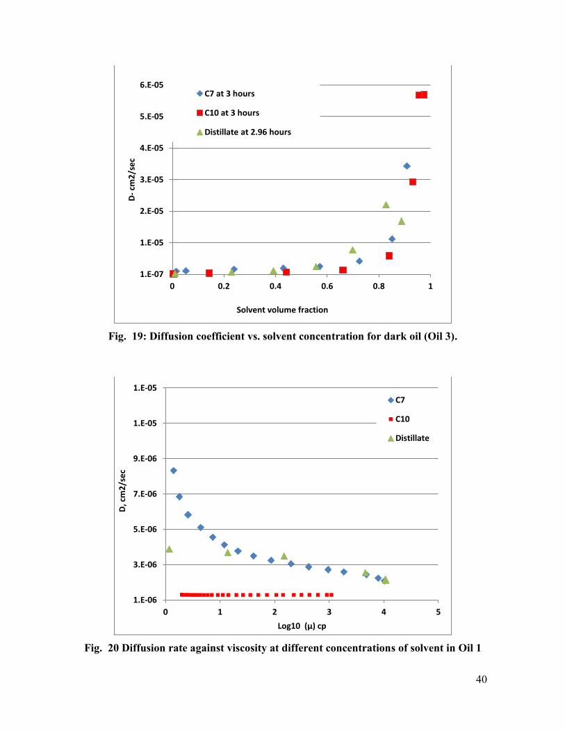
FIGURE 19: DIFFUSION COEFFICIENT VS. SOLVENT CONCENTRATION FOR
DARK OIL (OIL 3) .................................................................................................... 40
FIGURE 20: DIFFUSION RATE AGAINST VISCOSITY AT DIFFERENT
CONCENTRATIONS OF SOLVENT IN OIL 1 ....................................................... 40
Page 10
x
FIGURE 21: DIFFUSION RATE AGAINST VISCOSITY AT DIFFERENT
CONCENTRATIONS OF SOLVENT IN OIL 2. ...................................................... 41
FIGURE 22: DIFFUSION RATE AGAINST VISCOSITY AT DIFFERENT
CONCENTRATIONS OF SOLVENT IN OIL 3. ...................................................... 41
FIGURE A 1: DENSITY AT DIFFERENT CONCENTRATIONS OF SOLVENT IN
OIL………………………………………………………………………………… 142
FIGURE A 2: DENSITY AT DIFFERENT CONCENTRATION OF SOLVENT IN OIL 2.
..................................................................................................................................... 42
FIGURE A 3: DENSITY AT DIFFERENT CONCENTRATIONS OF SOLVENT IN OIL
3. .................................................................................................................................. 43
FIGURE A 4: VISCOSITY AT 25 °C FOR DIFFERENT CONCENTRATIONS OF
SOLVENT IN OIL 1 ................................................................................................... 43
FIGURE A 5: VISCOSITY AT 50 °C FOR DIFFERENT CONCENTRATIONS OF
SOLVENT IN OIL 3. .................................................................................................. 44
FIGURE A 6: VISCOSITY AT 25 °C FOR DIFFERENT CONCENTRATIONS OF
SOLVENT IN OIL 3 ................................................................................................... 44
FIGURE A 7: VISCOSITY AT 50 °C FOR DIFFERENT CONCENTRATIONS OF
SOLVENT IN OIL 1 ................................................................................................... 45
FIGURE A 8: VISCOSITY AT 50 °C FOR DIFFERENT CONCENTRATIONS OF
SOLVENT IN OIL 2. .................................................................................................. 45
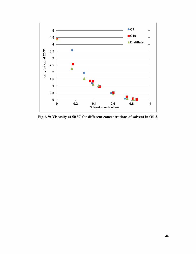
FIGURE A 9: VISCOSITY AT 50 °C FOR DIFFERENT CONCENTRATIONS OF
SOLVENT IN OIL 3 ................................................................................................... 46
CHAPTER 3........................................................................................................................47
FIGURE 1: BOILING RANGE DISTRIBUTION OF OIL SAMPLES AND DISTILLATE
.................................................................................................................................. 60
FIGURE 2: A—BEREA SANDSTONE CORE SATURATED WITH HEAVY OIL, B)
BEGINNING OF THE SOLVENT SOAKING EXPERIMENT, AND C)
CHANGED IN THE COLOR OF THE SURROUNDING FLUID (OIL SOLVENT
MIXTURE) DUE TO DIFFUSION PROCESS AT SOAKING TIMES >150
HOURS. ...................................................................................................................... 61
Page 11
xii
FIGURE 3: CORES AND SOLVENT HEATED TO SETTLED TEMPERATURE, B)
MEASURED CORE CHANGE WEIGHT, C) CORE AND SOLVENT PLACED IN
CONTACT AT THE SAME TEMPERATURE IN A SEALED IMBIBTION CELL,
D) SOAKING TEST RUN AT DETERMINED TEMPERATURE AND
REFRACTIVE INDEX TAKEN PERIODICA .......................................................... 61
FIGURE 4: RECOVERY RATES FOR OIL 1: EXPERIMENTS 4,5 AND 6 .................... 61
FIGURE 5: RECOVERY RATES FOR OIL 2: EXPERIMENTS 7, 8 AND 9. ................. 63
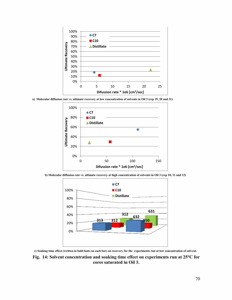
FIGURE 6: RECOVERY RATES FOR OIL 3: EXPERIMENTS 10, 11 AND 12. ............ 63
FIGURE 7: RECOVERY RATES FOR MINERAL OIL: EXPERIMENTS 1,2 AND 3. .. 63
FIGURE 8: RECOVERY RATES FOR CORES SATURATED WITH OIL 1 FOR
EXPERIMENTS RUN AT A) 25°C, B) 50°C AND C) 80°C .................................... 64
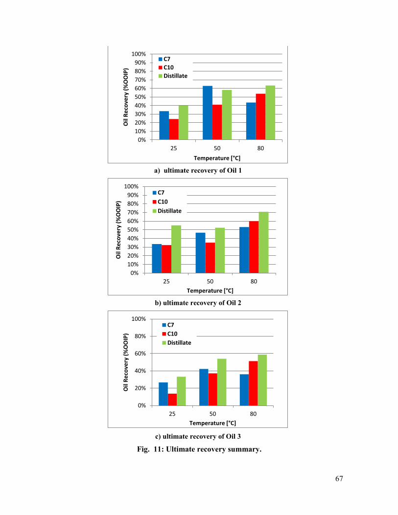
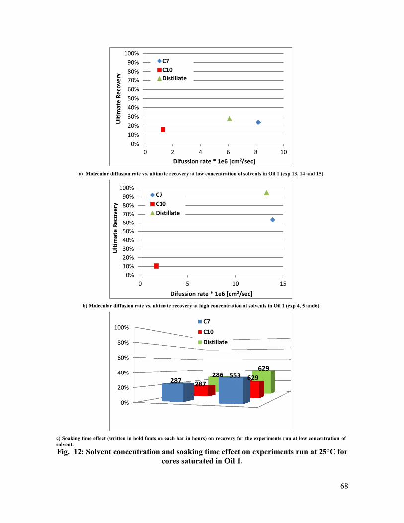
FIGURE 11: ULTIMATE RECOVERY SUMMARY ........................................................ 67
FIGURE 13: SOLVENT CONCENTRATION AND SOAKING TIME EFFECT ON
EXPERIMENTS RUN AT 25°C FOR CORES SATURATED IN OIL 2 ................. 69
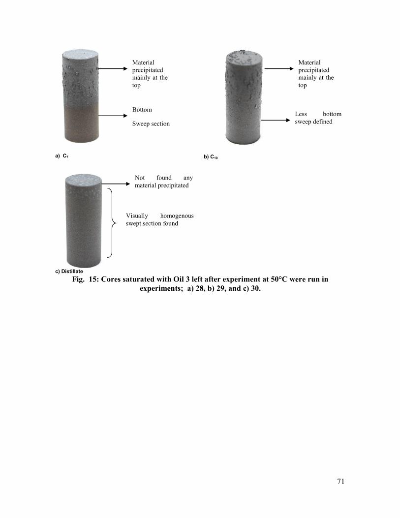
FIGURE 15: CORES SATURATED WITH OIL 3 LEFT AFTER EXPERIMENT AT
50°C WERE RUN IN EXPERIMENTS; A) 28, B)29 AND C)30 ............................ 71
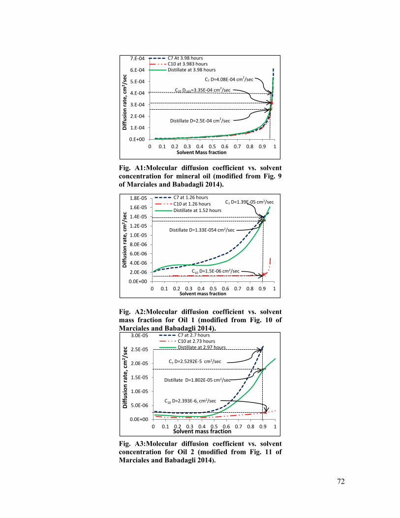
FIGURE A1: MOLECULAR DIFFUSION COEFFICIENT VS. SOLVENT
CONCENTRATION FOR MINERAL OIL (MODIFIED FROM FIG. 9 OF
MARCIALES AND BABADAGLI 2014). ................................................................ 72
FIGURE A2: MOLECULAR DIFFUSION COEFFICIENT VS. SOLVENT MASS
FRACTION FOR OIL 1 (MODIFIED FROM FIG. 10 OF MARCIALES AND
BABADAGLI 2014). .................................................................................................. 72
FIGURE A3: MOLECULAR DIFFUSION COEFFICIENT VS. SOLVENT
CONCENTRATION FOR OIL 2 (MODIFIED FROM FIG. 11 OF MARCIALES
AND BABADAGLI 2014). ........................................................................................ 72
CHAPTER 4........................................................................................................................73
FIGURE 1. MICROMODEL SCHEME AND PICTURE AREA. ...................................... 90
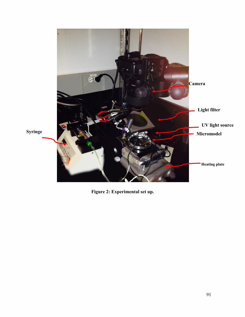
FIGURE 2. EXPERIMENTAL SET UP. ............................................................................. 91
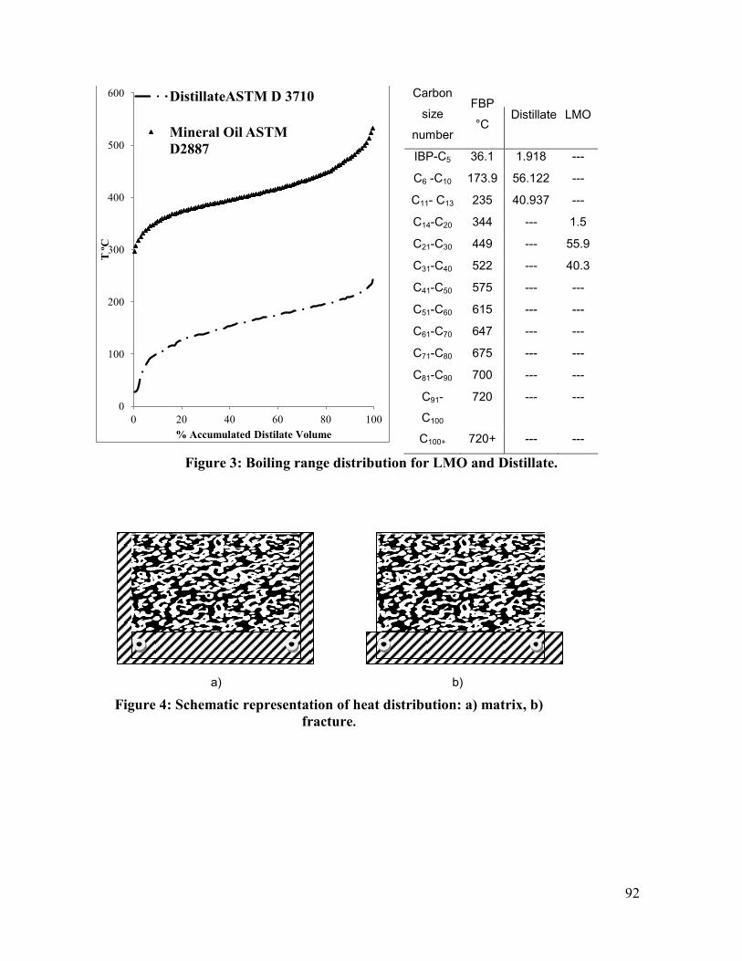
FIGURE 3. BOILING RANGE DISTRIBUTION FOR LMO AND DISTILLATE. ......... 92
FIGURE 4. SCHEMATIC REPRESENTATION OF HEAT DISTRIBUTION: A)
MATRIX, B) FRACTURE ....................................................................................... 92
Page 12
xiii
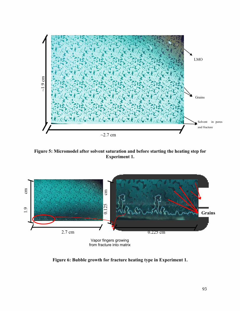
FIGURE 5. MICROMODEL AFTER SOLVENT SATURATION AND BEFORE
STARTING THE HEATING STEP FOR EXPERIMENT 1. .................................. 93
FIGURE 6. BUBBLE GROWTH FOR FRACTURE HEATING TYPE IN EXPERIMENT
1. ............................................................................................................................... 93
FIGURE 7. MACRO VISUALIZATION OF SOLVENT VAPORIZATION PATTERNS
FOR ALL THE EXPERIMENTS AT DIFFERENT TIMES. “0 MIN”
CORRESPONDS TO THE POINT FIRST BUBBLE IS OBSERVED .................. 94
FIGURE 8. SOLVENT RETRIEVAL MECHANISM. ....................................................... 95
FIGURE 9. MICROMODEL BEFORE SOLVENT PHASE CHANGE IN EXPERIMENT
3. ............................................................................................................................... 95
FIGURE 10. PHASE CHANGE OF SOLVENT WHEN HOMOGENEOUS (WHOLE
SYSTEM) HEATING IS APPLIED IN EXPERIMENT 3. ..................................... 96
FIGURE 11. RECOVERY MECHANISMS AND BUBBLE MIGRATION IN
EXPERIMENT 3. ..................................................................................................... 96
FIGURE 12. TIME EFFECT IN HOMOGENEOUS HEATING. ....................................... 96
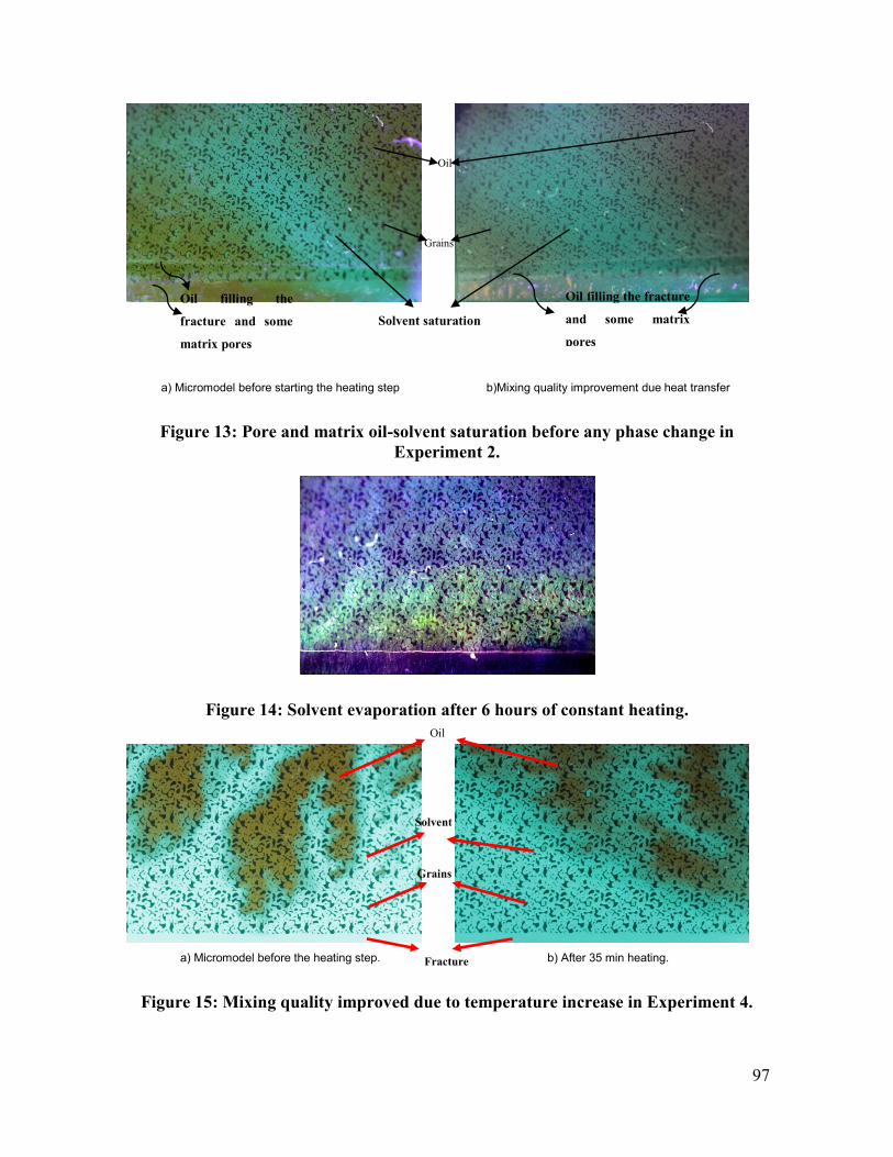
FIGURE 13. PORE AND MATRIX OIL-SOLVENT SATURATION BEFORE ANY
PHASE CHANGE IN EXPERIMENT 2. ................................................................ 97
FIGURE 14. SOLVENT EVAPORATION AFTER 6 HOURS OF CONSTANT
HEATING ................................................................................................................. 97
FIGURE 15. MIXING QUALITY IMPROVED DUE TO TEMPERATURE INCREASE
IN EXPERIMENT 4. ................................................................................................ 97
FIGURE 16. SOLVENT RECOVERY MECHANISM FOR EXPERIMENT 4. ............... 99
FIGURE 17. MATRIX OIL-SOLVENT MIXING BEFORE A) TEMPERATURE
INCREASE ANDB) PHASE CHANGE IN EXPERIMENT 5. .............................. 99
FIGURE 18. RECOVERY MECHANISM IN EXPERIMENT 5 ..................................... 100
FIGURE 19. WATER-WET VS. OIL-WET CASE........................................................... 100
FIGURE 20. VAPOR PHASE STABILITY WATER-WET (A AND B) VS. OIL-WET
CASE (C AND D). ................................................................................................. 101
Page 13
1
CHAPTER 1: INTRODUCTION
Page 14
2
Introduction
Alberta produced 76% of Canada´s oil equivalent production in 2013 with marked bitumen
representing 56% of this total. Meanwhile, Alberta’s ultimate potential recoverable
reserves were estimated to be 315 billion barrels of crude bitumen and only 5.4% of it has
been produced since its commercial production started in 1967 (AER 2014).
A great portion of the above-mentioned production (by in-situ recovery) has been achieved
by thermal methods, predominantly steam. Due to inefficiency of the steam injection
process, the use of different types of solvents (hydrocarbon and CO2) has been under
consideration for several decades as an alternative method to accelerate the viscosity
reduction process as well as in-situ upgrading.
The solvent injection was initially suggested as cold injection and different aspects of this
method were studied for a specific case called VAPEX (vapor extraction) (Butler and
Mokrys 1991, 1993). Due to its inefficiency (mainly cause by its high cost), the idea of
improving oil recovery led to combining it with thermal methods, either in the form of co-
injection with steam (Allen and Redford 1976; Farouq Ali and Abad 1973; Farouq Ali
1976; Das 1996a-b; Nasr et al. 2003, 2005; Li and Mamora 2011) or by alternate injection
(Zhao 2004; Zhao et al. 2005; Al-Bahlani and Babadagli 2011a-b, 2012; Pathak et al. 2011,
2012, 2013).
Despite numerous laboratory and computational analysis of different versions of solvent
injection, technical and economic concerns still exist causing delays in its
commercialization. An optimization of the process is required to minimize the cost and
maximize the recovery and its retrieval (Edmunds et al. 2009; Al-Gosayir et al. 2012a-b,
2013; Mohammed and Babadagli 2013). This complicated exercise is typically done to
reduce the amount of solvent used while maximizing its retrieval and oil recovery. Before
determining the optimal conditions by applying exhaustive optimization schemes, it is
necessary to select the most suitable solvent based on application (temperature, cyclic
injection, continuous injection), reservoir type (oil sands, fracture carbonates), and oil
Page 15
3
composition (viscosity, asphaltene content, density), as well as the cost and availability of
solvent (Naderi and Babadagli 2014a-b; Naderi et al. 2014).
In this optimization process, the primary task is to select the proper solvent for given
application conditions (temperature, injected amount), reservoir type, and oil composition
(Gupta and Picherack 2003; Naderi and Babadagli 2014a-b; Naderi et al. 2014), as well as
to understand the mechanisms for its retrieval after its use. This requires a selection process
that optimizes the recovery rate and ultimate recovery.
Statement of the Problem
It is a well-known fact that lower carbon number solvents (typically propane and butane)
yield a faster diffusion into oil and oil-saturated rocks (Al-Bahlani and Babadagli 2011a-b).
Therefore, higher carbon number solvents (from pentane up to C11-C15 carbon number
range distillate oil) are more preferable for better mixing; yielding higher ultimate recovery
with less asphaltene deposition (Naderi et al. 2014). But, with this type of “heavy”
solvents, the diffusion rate is much slower compared to the “lighter” ones.
Mixing quality is the other factor in solvent-oil systems and was primarily quantified by
evaluating the solvent effect on oil viscosity reduction while avoiding asphaltenes
precipitation. This standard of solvent evaluation was studied by transport industry, which
looks for the best solvent to ease transportation through pipelines by diluting heavy oil to
reduce its viscosity. It is recommended to use a diluent with sufficiently effective polar
components to reduce oil viscosity with minimal asphaltenes precipitation (Gateau et al.
2004). Correlations are also available for heavy-oil solvent mixtures to be used in different
process modeling purposes (Mehrotra 1992). Other works related to the solubility of
asphaltenes in n-alkanes were performed through heavy oil titration tests (Kolal et al. 1992;
Rassamdana et al. 1996; Buenrostro-Gonzalez et al. 2004). In these experiments, each
heavy oil-solvent pair was diluted at several ratios and different soaking times. Then, the
resulting mixture was passed through a filter paper that was rinsed with the n-alkanes
employed and dried to estimate the precipitated asphaltenes by weight difference.
Then, two critical properties of solvents need to be evaluated in solvent selection processes
for in-situ upgrading and effective heavy-oil/bitumen recovery:
Page 16
4
(1) Diffusion rate: the solvent’s ability to penetrate into the heavy oil, which will affect
the oil recovery rate, and;
(2) Mixing quality: the solvent’s ability to reduce oil viscosity minimizing asphaltene
precipitation, which will eventually affect the ultimate recovery.
In all solvent applications, the retrieval of expensive solvent is essential for the economics
of the process. Numerous experimental work at the core scale were presented to clarify the
physics (Al-Bahlani and Babadagli, 2011b) and optimal operation conditions (Al-Bahlani
and Babadagli, 2011a-b; Pathak et al. 2011, 2012, 2013; Naderi and Goskuner, 2014) of the
solvent retrieval process. Visual studies are needed to clarify the dynamics of the solvent
recovery at non-isothermal conditions and the reasons behind the solvent entrapment in the
matrix.
These aspects of solvent methods for heavy-oil recovery need to be studied from a fluid-
fluid (oil-solvent) interaction in porous media point of view. Then, it is prudential to
extend the study to core experiments in order to understand how the diffusion rate and
mixing quality affect oil recovery (carrying out solvent-rock tests) and to micromodels
(micro fluidic devices) in order to clarify the physics of the solvent retrieval process at the
pore scale via visualization. In these attempts, the following questions need to be answered:
(1) Temperature effect: Is there any optimal temperature that maximizes oil recovery
and minimizes the solvent cost?
(2) Which method is more efficient? Higher solvent concentration that is run for
shorter soaking time or higher soaking time with a smaller amount of solvent?
(3) What are the relative contributions of gravity and diffusion rate affecting the
recovery?
(4) What are the optimal conditions to minimize solvent entrapment during its retrieval
at the pore scale?
This research addresses these questions. In an attempt to provide answers, a step-by-step
procedure is established and summarized in the following section.
Page 17
5
Aims and Objectives
This research aims to perform the following objectives:
1. Establish a case of study to represent different sets of pairs combining:
solvent type
oil type
2. Determine bulk diffusion rate for each pair by:
developing an optical using UV light
applying x-ray cat (computer axial tomography)
3. Evaluate the mixing quality for each pair analyzing the effects of:
viscosity and density reduction
solvent concentration
asphaltene precipitation
4. Examine solvent performance at different temperatures in porous media evaluating:
recovery rate
ultimate recovery
solvent concentration
soaking time
5. Cross check solvent bulk properties to porous media efficiency between:
recovery rate - diffusion rate
ultimate recovery - mixing quality
6. In addition to the above listed aims mainly related to heavy-oil recovery by solvent
injection, clarification of the solvent retrieval process at the end of the process
using:
micro scale investigation of solvent retrieval under variable temperature
parametric analysis for different heating conditions and rock wettability
Page 18
6
Structure of the Thesis
This is a paper-based thesis and is composed of four chapters. The main body is constructed
from three papers that have been submitted or prepared for peer-reviewed journals.
Versions of Chapter 2 and Chapter 3 were presented at two conferences. Chapters 2 to 4
contain their own introduction, literature survey, results, conclusions, and references.
CHAPTER 1
This chapter provides an introduction to the thesis and an overview. Here, a brief
background about solvent evaluation in bulk and rock experiments are discussed.
After this, the statement of the problem, major objectives, and goals are
summarized.
CHAPTER 2
This chapter contains a study for fluid-fluid (oil-solvent) interactions. Two main
solvent selection criteria parameters—diffusion rate and mixing quality—are
considered to evaluate solvent injection efficiency at different temperatures. An
optical method under static conditions along with image processing techniques are
proposed to determine one-dimensional diffusivity of liquid solvent into a wide
range of oil samples. The ideal solvent types for different oil types are determined
using the results from the diffusion rate and mixing quality experiments.
CHAPTER 3
As a continuation of Chapter 2, this chapter investigates fluid-rock (solvent-oil-
sandstone) interactions. Sandstone samples saturated with three different heavy-oils
are exposed to solvent diffusion at static conditions at different temperatures.
Recovery rate and ultimate recovery (and asphaltenes left behind) controlled by the
diffusion rate and mixing quality are measured. Solvent-rock and liquid-liquid (from
Chapter 2) results are correlated. The ideal solvent types, representing the optimal
recovery rate and ultimate recovery, are determined for liquid solvents in the carbon
number range of C7 to C13, and heavy oil types with a viscosity range on different
orders of magnitude.
Page 19
7
CHAPTER 4
This chapter provides a pore scale investigation of solvent retrieval for
heterogeneous systems. Solvent diffused into tighter matrix from highly permeable
medium (fracture, wormholes, high permeability streaks) are retrieved by boiling.
The effects of temperature, wettability, and heating conditions on the retrieval
efficiency are investigated.
CHAPTER 5
This chapter contains the contributions and achievements of this thesis and also
provides recommendations for future work.
References
1. Al-Bahlani, A.M. and Babadagli, T. 2011a. Field Scale Applicability and Efficiency
Analysis of Steam-Over-Solvent Injection in Fractured Reservoirs (SOS-FR)
Method for Heavy-Oil Recovery. J. Petr. Sci. and Eng. 78: 338-346.
2. Al-Bahlani, A.M. and Babadagli, T. 2011b. SOS-FR (Solvent-Over-Steam Injection
in Fractured Reservoir) Technique as a New Approach for Heavy-Oil and Bitumen
Recovery: An Overview of the Method. Energy and Fuels 25 (10): 4528-4539.
3. Al-Bahlani, A.M. and Babadagli. 2012. Laboratory Scale Experimental Analysis of
Steam-Over-Solvent Injection in Fractured Reservoirs (SOS-FR) for Heavy-Oil
Recovery. J. Petr. Sci. and Eng. 84-85: 42-56.
4. Al-Bahlani, A.M. and Babadagli, T. 2012. Visual Analysis of Diffusion Process
During Oil Recovery Using Hydrocarbon Solvents and Thermal Methods. Chem.
Eng. J. (181 182): 557-569.
5. Alberta Energy Regulator (AER). ST98-2014: Alberta´s Energy Reserves 2013 and
Supply/Demand Outlook 2014-2023.
6. Al-Gosayir, M., Leung, J. and Babadagli, T. 2012a. Design of Solvent-Assisted
SAGD Processes in Heterogeneous Reservoirs Using Hybrid Optimization
Techniques. J. Can. Pet. Tech. 51 (6) 437-44.
7. Al-Gosayir, M., Babadagli, T., and Leung, J. 2012b. Optimization of SAGD and
Solvent Additive SAGD Applications: Comparative Analysis of Optimization
Techniques with Improved Algorithm Configuration. J. Petr. Sci. and Eng. (98-99):
61-68.
8. Al-Gosayir, M., Leung, J., Babadagli, T. et al. 2013. Optimization of SOS-FR
(Steam-Over-Solvent Injection in Fractured Reservoirs) Method Using Hybrid
Techniques: Testing Cyclic Injection Case. J. Petr. Sci. and Eng. 110: 74-84.
9. Allen, J.C. & Redford, A.D. 1976. Combination Solvent-Noncondensable Gas
Injection Method for Recovering Petroleum from Viscous Petroleum-Containing
Formations Including Tar Sad Deposits, US Patent No. 4,109,720.
10. Buenrostro-Gonzalez, E., Lira-Galeana,C., Gil-Villegas, A. et al. 2004. Asphaltene
Precipitation in Crude Oils: Theory and Experiments. AIChE Journal. 50 (10),
Page 20
8
2552-2570
11. Butler, A.M and Mokrys, I.J. 1993 Recovery of Heavy Oils Using Vaporized
Hydrocarbon Solvents: Further Development of the Vapex Process. J. of Canadian
Petr. Tech. 32: 56-62
12. Das, S.K. and Butler, R.M. 1996a. Countercurrent Extraction of Heavy Oil and
Bitumen. Paper SPE 37094 presented at the International Conference on Horizontal
Well Technology, Calgary, Alberta, Canada, 18-20 November.
13. Das, S.K. and Butler, R.M. 1996b. Diffusion Coefficients of Propane and Butane in
Peace River Bitumen. Can. J. Chem. Eng. 74: 986-992.
14. Edmunds, N., Maini, B., and Peterson, J. 2009. Advanced Solvent-Additive
Processes via Genetic Optimization. Paper PETSOC 2009-115 presented at
Canadian International Petroleum Conference (CIPC) 2009, Calgary, Alberta,
Canada, 16-18 June.
15. Farouq, A. and Snyder, S.G. 1973. Miscible Thermal Methods Applied to a Two-
Dimensional, Vertical Tar Sand Pack, With Restricted Fluid Entry. J. Can. Pet.
Tech. 12 (4): 22-26
16. Farouq, A. 1976. Bitumen Recovery from Oil Sands, Using Solvents in Conjunction
with Steam. J. Can. Pet. Tech. 15 (3).
17. Gateau, P., Hénaut, L., Barré, L. et al. 2004. Heavy Oil Dilution. Oil & Gas Science
and Technology 59 (5): 503-509.
18. Gupta, S. and Picherack, P. 2003. Insights into Some Key Issues with Solvent
Aided Process. J. Can. Pet. Tech. 43 (2): 54-61.
19. Kolal S., Najman J. and Sayegh, S. 1992.Measurement and Correlation of
Asphaltene Precipitation from Heavy Oils by Gas Injection. J. Can. Pet. Technol.
31 (04): 24-30
20. Li, W. and Mamora, D.D. 2011. Light-and Heavy-Solvent Impacts on solvent-
Aided-SAGD Process: A Low-Pressure Experimental Study. J. Can. Pet. Tech. 50
(4): 19-30.
21. Mehrotra, A.K., Sheika, H., and Pooladi-Darvish, M. 2006. An Inverse Solution
Methodology for Estimating the Diffusion Coefficient of Gases in Athabasca
Bitumen from Pressure-Decay Data. J. Pet. Sci. Eng. 53 (3-4): 189-202
22. Mohammed, M. and Babadagli, T. 2013. Efficiency of Solvent Retrieval during
Steam-Over-Solvent Injection in Fractured Reservoirs (SOS-FR) Method: Core
Scale Experimentation. Paper SPE -165528-MS presented at the SPE Heavy Oil
Conference, Calgary, AB, 11-13 June.
23. Naderi, K. and Babadagli, T. 2014a. Use of Carbon Dioxide and Hydrocarbon
Solvents During the Method of Steam-Over-Solvent Injection in Fractured
Reservoirs for Heavy-Oil Recovery From Sandstones and Carbonates. Accepted for
publication in SPE Res. Eval. and Eng. 2014.
24. Naderi, K. and Babadagli, T. 2014b. An Evaluation of Solvent Selection Criteria
and Optimal Application Conditions for the Hybrid Applications of Thermal and
Solvent Methods. Submitted to J. of Canadian Petr. Tech. 2014b (in review).
25. Naderi, K., Babadagli, T., and Coskuner, G. 2014. Bitumen Recovery by the SOS-
FR (Steam-Over-Solvent Injection in Fractured Reservoirs) Method: An
Experimental Study on Grosmont Carbonates. Energy and Fuels 27 (11): 6501-
6517.
26. Naderi, K., Babadagli, T., and Coskuner, G. 2014. Bitumen Recovery by the SOS-
Page 21
9
FR (Steam-Over-Solvent Injection in Fractured Reservoirs) Method: An
Experimental Study on Grosmont Carbonates. Energy and Fuels 27 (11): 6501-
6517.
27. Nasr, T.N., Beaulieu, G. Golbeck, H. et al. 2003. Novel Expanding Solvent-SAGD
Process “ES-SAGD”. Can. Pet. Tech. (technical note) 42 (1): 13-16.
28. Nasr, T.N. and Ayodele, O.R. 2005. Thermal Techniques for the Recovery of
Heavy Oil and Bitumen. Paper SPE 97488 presented at the SPE Int. Imp. Oil Rec.
Conf., Kuala Lumpur, Malaysia, 5-6 December.
29. Pathak, V., Babadagli, T. and Edmunds, N.R. 2011. Heavy Oil and Bitumen
Recovery by Hot Solvent Injection. J. Petr. Sci. and Eng., 78: 637-645.
30. Pathak, V., Babadagli, T. and Edmunds, N.R. 2012. Mechanics of Heavy Oil and
Bitumen Recovery by Hot Solvent Injection. SPE Res. Eval. and Eng., 15 (2): 182-
194.
31. Pathak, V., Babadagli, T. and Edmunds, N.R. 2013. Experimental Investigation of
Bitumen Recovery from Fractured Carbonates Using Hot-Solvents. J. of Canadian
Petr. Tech... 52 (4): 289-295.
32. Rassamdana H., Dabir B., Nematy, M. et al. 1996. Asphalt Flocculation and
Deposition: I. The Onset of Precipitation. AIChE Journal. 42 (1): 10-22
33. Zhao, L. 2004. Steam Alternating Solvent Process. Paper SPE 86957 presented at
the International Thermal Operations and Heavy Oil and Western Regional meeting,
Bakersfield, California, 16-18 March.
34. Zhao, L., Nasr, T., Huang, G., et al. 2005. Steam Alternating Solvent Process: Lab
Test and Simulation. J. Can. Pet. Tech. 44 (9): 37-43.
Page 22
10
CHAPTER 2: SOLVENT SELECTION CRITERIA BASED ON DIFFUSION RATE
AND MIXING QUALITY FOR DIFFERENT TEMPERATURE STEAM/SOLVENT
APPLICATIONS IN HEAVY-OIL AND BITUMEN RECOVERY
This paper is a modified and improved version of SPE 169291, which was submitted at the
SPE Conference held in Maracaibo, Venezuela, 21–23 May 2014. A version of this chapter
has been submitted to the Journal of Canadian Petroleum Technology.
Page 23
11
Preface
Heavy-oil and bitumen recovery requires high recovery factors to offset the extreme high
cost of investments and operations. Attention has been given to solvent injection for this
purpose and it has been observed that high recoveries are achievable when combined with
steam injection. Heavier (“liquid”) solvents (liquid at ambient conditions) are especially
becoming more popular due to availability and transportation. High oil prices allow the
application of this kind of technique if a proper design is made to retrieve the injected
solvent efficiently. “Liquid” solvents are advantageous as they yield a better quality
mixing (especially with very heavy-oils and bitumen) but a lower diffusion rate than lighter
solvents like propane or butane. Despite this understanding, there still is not a clear
screening criterion for solvent selection to mitigate both diffusion rate and the quality of the
mixture.
In this study, two main solvent selection criteria parameters—diffusion rate and mixing
quality—were considered to evaluate solvent injection efficiency at different temperatures.
An optical method under static conditions along with image processing techniques were
proposed to determine one-dimensional diffusivity of liquid solvent into a wide range of oil
samples in a capillary tube. This sampling range varied from 40 cp oil to 250 cp, for which
digital image treatment was developed. X-ray computerized tomography was applied for
heavier (and darker) oils (viscosity range of 20,000 cp to 400,000 cp). The diffusion
coefficients were then computed through non-linear curve fitting based on an optimization
algorithm to assure that the obtained values were in agreement with available analytical
solutions. Next, viscosity measurements and asphaltene precipitation for the same heavy-
oil/solvent mixtures were performed to determine the mixing quality. The ideal solvent
types for different oil types were determined using the results from the diffusion rate and
mixing quality experiments.
The experimental and semi-analytical outcome of this research would be useful in
determination of the best solvent type for given oil and in understanding the key factors that
influence the quality of mixtures including viscosity reduction and probable asphaltene
precipitation.
Page 24
12
1. Introduction
Solvent injection has been under consideration for several decades as an alternative method
for reducing heavy-oil/bitumen viscosity as well as upgrading it in-situ. Initially, it was
suggested as cold solvent injection and different studies were carried out considering
different types of hydrocarbon solvents (Butler and Mokrys 1991, 1993). Due to its high
cost for industrial applications, the idea of improving oil recovery led to combining it with
thermal methods either in the form of co-injection with steam (Allen and Redford 1976;
Farouq and Abad 1973; Farouq 1976; Das 1996a-b; Nasr et al. 2003, 2005; Li and Mamora
2011) or by alternate injection (Zhao 2004; Zhao et al. 2005; Al-Bahlani and Babadagli
2011a-b, 2012; Pathak et al. 2011, 2012, 2013).
Despite numerous laboratory and computational analysis of different versions of solvent
injection, technical and economic concerns still exist causing delays in its
commercialization. An optimization of the process is required to minimize the cost and
maximize the recovery and its retrieval (Edmunds et al. 2009; Al-Gosayir et al. 2012a-b,
2013; Mohammed and Babadagli 2013). This complicated exercise is typically done to
reduce the amount of solvent used while maximizing its retrieval and oil recovery. Before
determining the optimal conditions by applying exhaustive optimization schemes, it is
necessary to select the most suitable solvent based on application (temperature, cyclic
injection, continuous injection), reservoir type (oil sands, fracture carbonates), and oil
composition (viscosity, asphaltene content, density) as well as the cost and availability of
solvent (Naderi and Babadagli 2014a-b; Naderi et al. 2014).
In the solvent selection process, two factors play a critical role: (1) Diffusion rate, i.e., the
rate of solvent mass transfer into heavy oil, and (2) mixing quality, i.e., lowered viscosity
with minimal asphaltene precipitation. Historically, the tendency was to use lighter
solvents (propane, butane) in the form of gas (Butler and Mokrys 1991, 1993) in heavy-oil
recovery. However, despite its high diffusion rate, the mixing quality is low, causing
significant asphaltene deposition (Moreno and Babadagli 2014a-b). Because of this fact,
higher carbon number has been also tested in the form of gas (Nasr and Ayodele 2005;
Ayodele et al. 2010; Keshavarz et al. 2013) or liquid (Naderi et al. 2014). As the carbon
number of the solvent increases, the diffusion decreases but mixing be higher quality (Al-
Page 25
13
Bahlani and Babadagli 2011b; Coskuner et al. 2013). The mixing quality will be even
better if solvents with aromatic content (distillate oil, condensates, light oils) are used rather
than single component alkanes (Coskuner et al. 2013; Naderi et al. 2014).
As can be inferred from the above summary, detailed studies combining both factors—i.e.,
diffusion rate and mixing quality—are needed in the solvent selection process. Attention
was paid to the diffusion rate measurement in the past. These techniques are classified by
their ability to avoid any disturbance to the system during experimentation and, hence, can
be in the form of intrusive or non-intrusive experiments (Guerrero 2009). Non-intrusive
experiments were found to be more suitable to determine the solvent rate of penetration
since they minimize the errors when solvent concentration was measured (Guerrero and
Kantzas 2009). Different free diffusion techniques were developed for this purpose
depending on the solvent phase. Riazi (1996) proposed the pressure decay method for
diffusion rate calculation in heavy oil that uses an expression of gaseous solvent
concentration as a function of pressure decreasing inside the closed system caused by. This
method can be named “standard” when low molecular weight solvents are used (Guerrero
2009) and improved versions of this approach were also reported (Ghaderi et al 2011;
Zhang et al. 2000; Creux et al. 2005; Upreti and Mehrotra 2000; Mehrotra et al. 2006).
More recently, the Pendant Drop Shape Analysis (PDSA) was proposed as an improved
methodology, including the effect of oil swelling due to solvent penetration when a drop of
oil was pending in a closed medium surrounded by gaseous solvent (Yang and Gu 2003).
For liquid-liquid systems, different optical methods were also proposed. These methods
were based on the ability of the source and detectors implemented to register the spatial
solvent distribution while the experiment was running. Initially, Oballa and Butler (1989)
measured the diffusion rate of toluene into Cold Lake bitumen using laser and reported a
value on the order of 10-8
cm2/sec. Nuclear Magnetic Resonance (NMR) was also used for
the same purpose (Wen et al. 2005a-b). In this method, the T2 relaxation time of the
hydrocarbon samples in the NMR spectra were used to identify the solvent concentration in
the mixture, which varied in the range of 5-15% in weight. The reported diffusion rates of
heptane (C7), decane (C10), and distillate solvents in bitumen and heavy oil samples were on
the order of 10-7
to 10-9
cm2/sec. Recently, the application of X-ray scattering was found to
Page 26
14
be useful for measuring the mixing rates (Weng et al. 2004; Afshani and Kantzas 2007;
Guerrero 2009; Guerrero and Kantzas 2009).
With the exception of the PDSA (Yang and Gu 2003), all of these non-intrusive methods
used a closed system in which the heavy oil component was placed at the bottom and the
solvent was carefully injected on top. In this case, the interface of the system can be taken
as a reference point for further mathematical analysis in which the data was fitted into the
analytical solutions available in the literature. This problem was found to be
mathematically described as one dimensional diffusing solvent in a static closed vial. In
other words, there is no mass transfer with the environment, the interface between solvent
and oil is fixed, there is no change in global volume, and Fickian diffusion occurs only in
one direction. This means that the mass flow from the solvent to solute (oil) is only due to
the concentration gradient. These statements are summarized mathematically as mass
transfer problem in an extended initial distribution medium as follows (Crank 1975; Bird et
al. 2001):
(1)
where:
At t = 0
For (above the oil interface) and for ,
For t > 0,
at ,
x direction is increasing downwards.
The analytical solution to this system leads to the following (Crank 1975):
(2)
This equation describes the concentration profile along the axial axe of the vial at different
times with an average diffusion coefficient and gives an idea about the rate or ability of the
specified solvent to penetrate into heavier hydrocarbon. The magnitude of this parameter is
[length2/ time] and for the solvents employed in this study, the diffusion coefficient values
Page 27
15
fall into a range between 10-5
to 10-8
cm2/sec (Guerrero 2009; Wen et al 2005a; Wen et al.
2005b) at 25 °C, depending on the system in consideration.
Mixing quality is the other factor in solvent-oil systems and was primarily quantified by
evaluating the solvent effect on oil viscosity reduction while avoiding asphaltenes
precipitation. This standard of solvent evaluation was studied by transport industry, which
looks for the best solvent to transport heavy oil through pipelines by reducing viscosity. It
is recommended to use a diluent with sufficiently effective polar components to reduce oil
viscosity with minimal asphaltenes precipitation (Gateau et al. 2004). Correlations are also
available for heavy-oil solvent mixtures to be used in different process modeling purposes
(Mehrotra 1992). Other works related to the solubility of asphaltenes in n-alkanes were
performed through heavy oil titration tests (Kolal et al. 1992; Rassamdana et al. 1996;
Buenrostro-Gonzalez et al. 2004). In these experiments, each heavy oil-solvent pair was
diluted at several ratios and different soaking times. Then, the resulting mixture was passed
through a filter paper that was rinsed with the n-alkanes employed and dried to estimate the
precipitated asphaltenes by weight difference.
The present study focuses on selection of proper solvents by cross-checking the diffusion
(mixing) rate and mixing quality. A combination of four heavy oil types and three solvents
with a wide range of viscosities and densities were used to provide a general framework.
Diffusion experiments were performed using UV lights and X-ray CAT. To test the mixing
quality, viscosity and asphaltene precipitation measurements were carried out for different
oil-solvent mixtures. Using this data with diffusion rate measurements, a selection of proper
solvent type for a wide variety of heavy oils is presented.
2. Experimental Methodology
2.1 Materials.
A case of study was established to understand and evaluate solvent selection criteria for
heavy-oil recovery processes. Three different solvents and four different oil samples were
selected to achieve this objective: Light mineral oils (LMO) and heavy mineral oils (HMO)
and three crude oils (Oil 1, Oil 2, and Oil 3) obtained from three different fields in Alberta,
Page 28
16
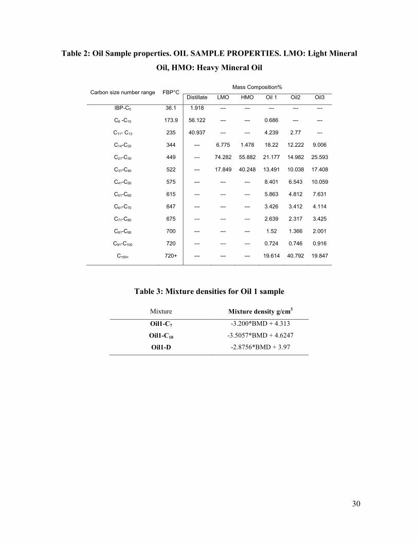
Canada. The solvent and oil samples are summarized in Tables 1 to 3. The viscosity data
for heptane and decane given in Table 1 were taken from literature (Dymond and Oye
1993). Figure 1 shows their boiling range distribution obtained through gas chromatograph
(GC) analysis under specified standards, which is also specified in Table 3.
3. Free Diffusion Experiments
Diffusion experiments are designed to generate the change in the concentration profile
when two miscible fluids are in contact and require proper visualization technique. Because
the processed oil samples (mineral oils in Table 2) are transparent, optical techniques are
applicable. For heavy oil samples (Oil 1, Oil 2, and Oil 3 in Table 2), however, one has to
take advantage of advanced visualization techniques such as X-ray CAT or nuclear
magnetic resonance (NMR). The procedure and observations are summarized below.
3.1 Free diffusion experiments with mineral oil samples.
When the mineral oil was employed inside a capillary tube, the concentration of the -dyed-
solvent inside the mixture was tracked by measuring its pixel intensity using a digital
camera. For these experiments, the solvents were dyed with yellow fluorescent color
DFSB-K43 (Risk Reactor Inc. 2005) composed of n-butyl-4-(butylamino) 1, 8-
naphthalalimide – FUROL 555 (Curtis and Nikiforos 2006), which was excited by a 405
nm UV LED of 5610 lumen inside a dark box. A CANON 7D camera with a 50 mm lens
was set at a 3’’2 shutter speed and 4.5 aperture. To avoid possible noises, a S-W 040 -
Orange 550 (Schneider Optische 2007) filter was used to simply block possible blue lights
allowing only red and yellow lights to pass through the lens.
Initially, the standard patterns of different pixel intensities were created for various solvent
concentrations. In this process, 0wt%, 30wt%, 50wt%, 70wt%, and 100wt% solvent
concentrations in the mixtures were registered and the pixel intensities in red, green, blue
(RGB) colors were measured using MATLAB®. Then, statistical analyses were performed
to minimize the standard deviation in quantification of pixel values for various solvent
concentrations. Next, the capillary tubes were filled with mineral oil from the bottom by
capillary imbibition until its level reached a certain height. The solvent was injected very
carefully at the top of the capillary tube using a 29G needle to assure it comprises 20wt% of
Page 29
17
the total amount of fluids in the tube. Finally, the tubes were sealed with epoxy resin to
avoid any solvent loss and were placed carefully in the dark box in vertical position. The
camera was programmed to take images every hour for a minimum of 10 hours. Further
analysis of the images collected was carried out in the MATLAB®
environment.
3.2 Free diffusion experiments with dark oil samples.
As a quick and nondestructive method for three-dimensional visualization and
characterization of opaque objects, high-resolution X-ray computed tomography (CT) was
selected as a methodology to determine the diffusion rate for crude oil samples. This
technique differs from conventional medical CAT scanning in the resolution of the
information obtained, which is up to a few microns in size. This technique has been applied
successfully in medicine and further extended to geosciences (Ketcham 2001). The success
of the application of this methodology requires the proper configuration of micro-CT
scanner, in terms of X-ray energy, image resolution, and attenuation vs. density calibration.
In our experiments, a SkyScan1176 micro CT scanner was employed using image pixel size
35 µm at 35kv to obtain the average attenuation coefficient for each pure sample. The X-
ray attenuation was calibrated using a commercially standardized phantom (a material
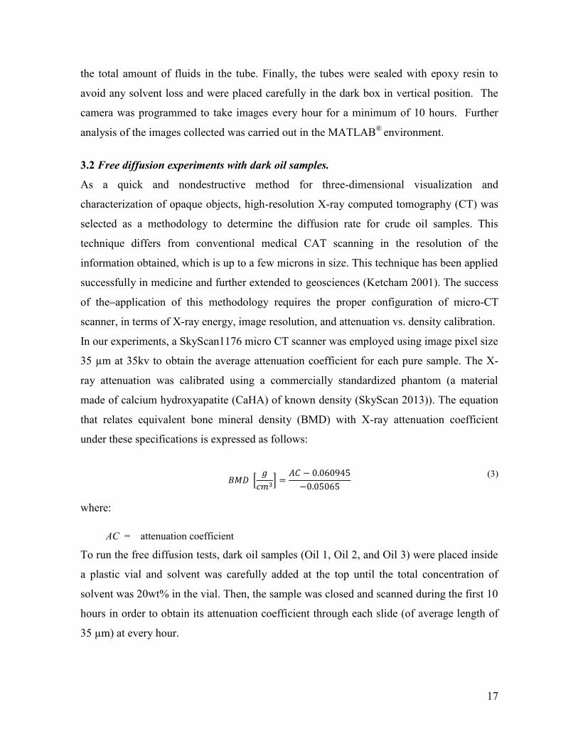
made of calcium hydroxyapatite (CaHA) of known density (SkyScan 2013)). The equation
that relates equivalent bone mineral density (BMD) with X-ray attenuation coefficient
under these specifications is expressed as follows:
(3)
where:
AC = attenuation coefficient
To run the free diffusion tests, dark oil samples (Oil 1, Oil 2, and Oil 3) were placed inside
a plastic vial and solvent was carefully added at the top until the total concentration of
solvent was 20wt% in the vial. Then, the sample was closed and scanned during the first 10
hours in order to obtain its attenuation coefficient through each slide (of average length of
35 µm) at every hour.
Page 30
18
4. Obtaining the Concentration Profiles of Mineral Oil Samples
To calculate the diffusion rate, it is necessary to obtain the concentration profiles. This
depends on the ability of the employed technique to differentiate the solvent from the oil in
the system while it is diffusing into each other.
4. 1 Mineral oil samples (optical method).
In order to quantify the concentration profile, the images obtained from the experiments at
different times were treated by applying the following steps:
1. The entire capillary tube was selected from the picture.
2. The green pixel intensity was averaged for each line in the abscissa along the length
of the tube.
3. Each averaged value was normalized between 0 and 1 after using the following
equation (Spotfire 2012):
(4)
where:
original pixel intensity (G)
normalized value (scaled between 0 and 1)
minimum value for obtained pixel intensity
maximum value for obtained pixel intensity
4. Each normalized value was transformed into weight percent solvent concentration.
Table 4 summarizes the obtained values through this procedure.
5. The units from coordinate axis were transformed from pixel scale to centimeter
scale based on the distance from the camera to the objectives.
6. Finally, the concentration profiles were obtained.
Note that proper combination of camera filter and dye color was chosen to obtain the best
color identification of the present phases. Figure 2 shows the capillary tube and the
intensity-concentration profiles of the LMO-C7 case after applying steps 1 to 6 using
MATLAB®. In this particular example, the red and blue distributions are also shown with
Page 31
19
their corresponding colors. The green trend is more useful to recognize the solvent from
oil compared to the blue and red trends as the wavelength emission of this dye is around
500 nm (Curtis and Nikiforos 2006), showing a green-yellow color shade (Risk Reactor
Inc. 2005), and the filter used blocks mainly all light emissions below 500 nm (Schneider
Optische 2007).
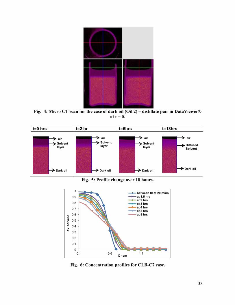
4. 2 Dark (crude) oil samples (X-ray CAT).
All scanned samples were initially reconstructed using the standardized phantom as
reference. Subsequently, the portion of the vial to be analyzed was selected in the
DataViewer® software (Figs. 4 and 5) and the equivalent density was obtained for sections
of 0.1 mm length. Eq. (3) was applied on a group of 33 slices inside the vial, each 35 µm in
average, using the CTan® software. The equivalent density was then transformed into
mixture density by correlating the BMD to the oil-solvent pair. Table 4 describes the
BMD-Oil density correlation employed for Oil 1. Figure 6 shows the concentration profile
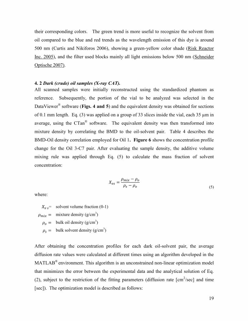
change for the Oil 3-C7 pair. After evaluating the sample density, the additive volume
mixing rule was applied through Eq. (5) to calculate the mass fraction of solvent
concentration:
(5)
where:
= solvent volume fraction (0-1)
mixture density (g/cm3)
bulk oil density (g/cm3)
bulk solvent density (g/cm3)
After obtaining the concentration profiles for each dark oil-solvent pair, the average
diffusion rate values were calculated at different times using an algorithm developed in the
MATLAB®
environment. This algorithm is an unconstrained non-linear optimization model
that minimizes the error between the experimental data and the analytical solution of Eq.
(2), subject to the restriction of the fitting parameters (diffusion rate [cm2/sec] and time
[sec]). The optimization model is described as follows:
Page 32
20
Min err =
s.t. 1e-8 1e-3
where:
err error function,
concentration profile; i.e., solvent mass fraction vs. x-cm data obtained from the
experiments,
concentration profile in the same units as calculated from the optimized D
and t,
time - sec from the start of the experiment that better fits the analytical solution for
objective function minimization, which can vary from a very short period –c or +c,
less than 10% of the time from which the data was obtained,
diffusion rate - cm2/sec that better fits the analytical solution in Eq. (2). For this case,
diffusion rate boundaries were left as wide as possible for less biased data.
After finding the average diffusion rate at each time, the concentration dependency of
diffusion rate was determined applying the procedure proposed by Sarafianos (1996) and
Guerrero (2009) using the following equations:
(6)
(7)
(8)
(9)
(10)
Sarafianos (1996) indicated that in Eq. (6) correspond to 100% of the diffusing
component, which was metal for his experiments. Guerrero (2009) proposed a methodology
Page 33
21
using Eqs. (6) through (10) to obtain the diffusion rate as a function of solvent
concentration. The first step in this procedure is to obtain the concentration profile to
estimate the term in Eq. (6). Here, u is an introduced function that relates the
spatial distribution of the concentration profile and can be obtained from the inverse
calculation of the error function using Eq. (6) or by the employment of Eq. (7). At the next
step, it is necessary to plot u against the spatial distribution (x) in order to find the
relationship described by Eq. (8). In this equation, h is the slope and k is the tangent
intercepting the ordinate axis and they should be determined at each point of u vs. x pair.
Finally, Eq. (10) is used to estimate the diffusion coefficient for different solvent
concentrations.
5. Mixture Quality Evaluation by Viscosity Measurements and Asphaltene Titration
Tests
The efficiency of solvent was evaluated through its ability to reduce oil density and
viscosity with minimum asphaltene precipitation. The precipitated asphaltene by each
solvent was measured with titration tests as described in literature (Kokal et al. 1992;
Rassamdana et al. 1996; Buenrostro-Gonzalez et al. 2004). In our case, 5 grams of each
dark oil sample were mixed at room conditions and different proportions with specified
solvents in Table 2. The resulting mixture went through 24 hrs of soaking in a closed
system and then was filtered under vacuum using a filter paper Watman No. 42. The paper
was rinsed with the corresponding n-alkane in order to isolate the insoluble material from
oil and further dried for solvent evaporation. The weight difference in the filter paper was
correlated to the precipitated material associated with asphaltenes. The distillate used to
rinse the oil mixtures was filtered through a column employed for SARA analysis to
remove the aromatic composition and better evaluate its impact on minimizing asphaltene
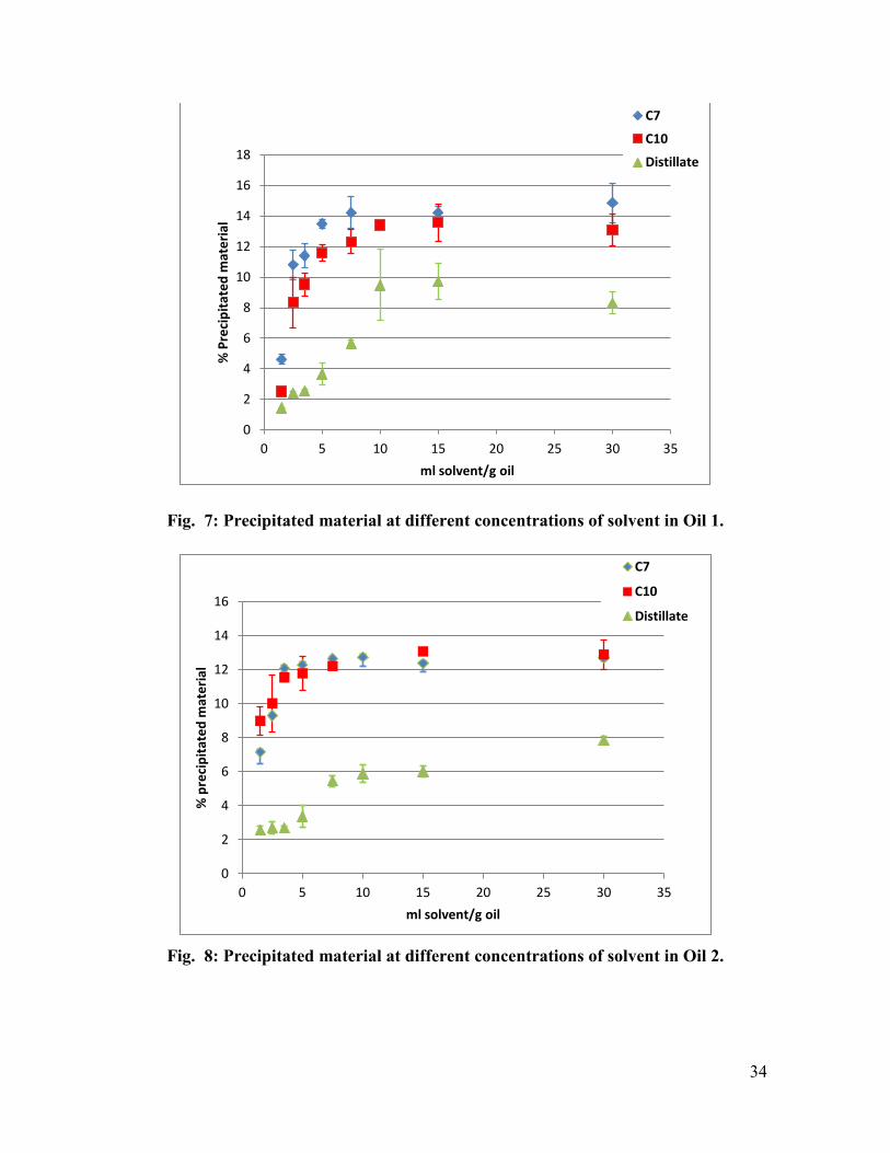
precipitation. Figures 7 to 9 show the results for Oil 1, 2, and 3 with solvents at different
proportions.
The density and viscosity of dark oil solutions (20, 40, 60, and 80 wt% of solvent) were
also measured. Densities were obtained at 25°C by a DDM 2910 Density Meter while the
viscosities were measured at different temperatures using a Brookfield Programmable
Page 34
22
LVDV-II+ Viscometer. Examples of density and viscosity changes with solvent
concentrations in the mixture are given in the Appendix.
6. Solvent Selection Considering Diffusion Rate and Mixing Quality
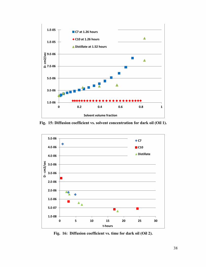
Figures 10 to 19 illustrate the calculated values of diffusion rate at different times using
Eq. (2) and its variation with concentration in accordance to the set of Eqs. (6) through
(10). The single component cases (C7 and C10) followed a typical trend (an exponential
change of the diffusion coefficient with time and solvent concentration) and, as expected,
the lower the carbon number of solvent, the faster the solvent diffusion. These results are in
agreement with the observations of Wen (2004), Guerrero (2009), and Guerrero and
Kantzas (2009). A similar trend was also observed for the distillate cases with LMO and
HMO (Figs. 10 through 13). However, in the cases of dark oil (Oil 1 and Oil 2), though the
lightest solvent (C7) followed an exponential trend, the heavier solvents (C10 and distillate)
yielded very weak diffusion responses with respect to time (Figs. 13 and 16). Diffusion
coefficient did not change for Oil 1 (14) as time passed. As illustrated in Figures 14 and
15, C10 did not show any changes in the diffusion process even at high solvent
concentrations. The same behavior was observed for the distillate case at early times;
however, in this case, increasing solvent concentration resulted in an increase in the
diffusion coefficient at late times. This could be attributed to the multi component nature
of the distillate. In fact, this particular solvent contains aromatic compounds that are
capable of dissolving asphaltenes, which eventually provides better mixing conditions. For
the case of Oil 3, C7 and distillate diffusion rates were observed to be close to each other
(Fig. 18), but distillate showed a faster diffusion than C7 at high solvent concentrations, as
seen in Figure 19.
This characteristic behavior implies that distillate can be as effective as light hydrocarbon
solvents (C7 in our case) in the long run. It might also be suggested to start the process
with lighter solvents to take advantage of its high diffusion capability and subsequently
continue with distillate type solvent, which is relatively inexpensive and readily available.
Page 35
23
Another important issue to be addressed is the soaking time. It was observed that diffusion
rate decreases as the soaking time increases. This is mainly due to a significant change in
the quality of the present solvent at its interface with heavy oil, as the global concentration
of solvent is constant during our experiment. This is in agreement with other observations
(Zhang 2000; Wen 2004) and might necessitate the replenishing of solvent in cyclic
stimulation type applications for a more effective diffusion process.
Figures 7 to 9 show the solvent efficiency in terms of asphaltene precipitation. This, in turn,
would affect ultimate recovery when implemented in the reservoir. In our case, the least
viscous dark Oil (Oil 1, Fig. 7) was found to precipitate the same amount of asphaltenes
compared to the most viscous one (Oil 3, Fig. 9) at identical solvent ratios. This
phenomenon might be explained with the proportional presence of resins/asphaltenes in the
oil, which would determine the effect of crude composition and make the oil prone to
precipitation as suggested by Kokal (1992).
It can also be observed that after the concentration of solvent in the mixture is higher than
10 cm3/g oil, the precipitated amount increased. This is also in line with previous
observations (Kolal et al. 1992; Rassamdana et al. 1996; Buenrostro-Gonzalez et al. 2004).
Although experiments were carried out at atmospheric pressure, this asymptotic behavior at
different solvent ratios was also observed at higher pressures (Akbarzadeh et al. 2004;
Sabbagh et al. 2006). This would imply that when the solvent is applied inside the
reservoir, there could be regions of high solvent concentration in which asphaltene
precipitation would be at maximum and could cause pore blockage and reservoir
impairment. Therefore, it is important to take asphaltene precipitation as an index of
solvent quality into consideration.
As a general trend for the n-alkane case, it was found that C7 precipitates less material
compared to C10; i.e., the lower the carbon number, the lower the precipitated material as
in agreement with earlier observations (Kokal et al. 1992; Rassamdana et al. 1996;
Buenrostro-Gonzalez et al. 2004; Moreno and Babadagli 2014a-b). In this study, the
distillate was found to be the best solvent in terms of minimum asphaltene precipitation.
Page 36
24
Again, this is due to the presence of aromatic components, which would lead to better
asphaltene dilution in the mixtures.
As iteratively mentioned throughout the paper, the two characteristics that are critically
important in solvent applications are (1) diffusion rate and (2) mixing quality. Figures 20
to 22 present a cross-plot to indicate the impact of solvent concentration on both diffusion
rate and viscosity reduction. As can be observed, an exponentially declining trend in
viscosity accompanies the decreasing trend of diffusion coefficients, which is in agreement
with previous observations by Das and Butler (1996b). The desirable region is high
diffusion rate, low mixture viscosity, and low solvent concentrations. Initially, C7 appears
to be the best solvent considering all three parameters but the distillate exhibits a similar
trend to C7. The plots given in Figures 20 and 22 also verify the previous suggestion of
starting the process with a light solvent and continuing with less expensive distillate.
7. Conclusions
(1) An image processing and analysis scheme was developed to measure the diffusion rate
for different heavy-oil-solvent pairs. Optical and high resolution X-ray CAT methods
were applied for transparent (mineral oils) and opaque (crude -dark- oil) oil samples,
respectively. For both cases, the diffusion rate decreased when the carbon number of
the solvent increased while also depending on time. In fact, the diffusion rate dropped
down two orders of magnitude in later times suggesting that the most effective solvent
application would occur in the early stages and the solvent should be replenished after
this period.
(2) For the light (LMO and HMO) and dark (Oil 1 and Oil 2) oil cases, the diffusion rate
was found to be strongly dependent on solvent concentration; i.e., it is an increasing
monotonic function of solvent concentration, indicating that higher amounts of solvent
would be needed for higher diffusion rates.
(3) Solvent concentration affects not only the diffusion rate but also the quality of mixture.
It was observed as an exponentially declining trend in viscosity when diffusion
coefficient was in a decreasing trend.
Page 37
25
(4) For the light mineral oil cases, diffusion rate was not found to be strongly dependent on
solvent concentration, contrary to the dark oil case, in which a different trend was
obtained.
(5) Additionally, for the dark oil cases (Oil 1 and Oil 2), it was found that when solvent
concentration increases up to 0.2 mass fraction at the interface of the mixture, diffusion
rate increases up to one order of magnitude, suggesting that the most effective solvent
application would be through the short periods of solvent replenish in which overall
solvent concentration in the mixture is quite low.
(6) Distillate is as fast as C7 in Oil 3, especially at high solvent concentrations.
(7) In general, it was found for our cases that optimal solvent concentration falls in the
range of 0.2 to 0.4 volume in the mixture because, at this concentration of solvent in
the mixture, oil viscosity decreases dramatically (about half of the original value),
diffusion rate is quite high and asphaltene precipitation is minimum.
(8) The distillate and C7 are the best candidates to be used as solvents when both diffusion
rate and mixing quality were considered. However, considering the asphaltene
dissolving capability, distillate could be as effective as light single component solvents
at late stages. Then, one may suggest starting the process with lighter solvents to take
advantage of its high diffusion capability and continue with distillate type solvent,
which is relatively inexpensive and readily available.
Acknowledgements
This research was conducted under the second author’s (TB) NSERC Industrial Research
Chair in Unconventional Oil Recovery (industrial partners are CNRL, SUNCOR,
Petrobank, Sherritt Oil, APEX Eng., PEMEX, Husky Energy, and Statoil). A partial
support was also obtained from an NSERC Discovery grant (No: RES0011227). We
gratefully acknowledge these supports.
Appendix
Page 38
26
Examples of density and viscosity changes with solvent concentrations in the mixture
Figures A1-A9.
References
1. Akbarzadeh, K., Sabbagh, O. , Beck, J. et al. 2004. Asphaltene Precipitation from
Bitumen Diluted With n-Alkanes. Paper presented at the Canadian International
Petroleum Conf., Calgary, Alberta, Canada, 8-10 June.
2. Allen, J.C. and Redford, A.D. 1976. Combination Solvent-Noncondensable Gas
Injection Method for Recovering Petroleum from Viscous Petroleum-Containing
Formations including Tar Sad Deposits. US Patent No. 4,109,720.
3. Afshani, B. and Kantzas, A. 2007. Advances in Diffusivity Measurement of
Solvents in Oil Sands. J. Can. Pet. Tech. 46 (11): 56-61.
4. Al-Bahlani, A.M. and Babadagli, T. 2011a. Field Scale Applicability and
Efficiency Analysis of Steam-Over-Solvent Injection in Fractured Reservoirs
(SOS-FR) Method for Heavy-Oil Recovery. J. Petr. Sci. and Eng. 78: 338-346.
5. Al-Bahlani, A.M. and Babadagli, T. 2011b. SOS-FR (Solvent-Over-Steam
Injection in Fractured Reservoir) Technique as a New Approach for Heavy-Oil
and Bitumen Recovery: An Overview of the Method. Energy and Fuels 25 (10):
4528-4539.
6. Al-Gosayir, M., Leung, J. and Babadagli, T. 2012a. Design of Solvent-Assisted
SAGD Processes in Heterogeneous Reservoirs Using Hybrid Optimization
Techniques. J. Can. Pet. Tech. 51 (6) 437-44.
7. Al-Gosayir, M., Babadagli, T., and Leung, J. 2012b. Optimization of SAGD and
Solvent Additive SAGD Applications: Comparative Analysis of Optimization
Techniques with Improved Algorithm Configuration. J. Petr. Sci. and Eng. (98-
99): 61-68.
8. Al-Gosayir, M., Leung, J., Babadagli, T. et al. 2013. Optimization of SOS-FR
(Steam-Over-Solvent Injection in Fractured Reservoirs) Method Using Hybrid
Techniques: Testing Cyclic Injection Case. J. Petr. Sci. and Eng. 110: 74-84.
9. Ayodele, O. R., Nasr, T.N., Ivory, J. et al. 2010. Testing and History Matching ES-
SAGD (Using Hexane). Paper SPE 134002 presented at the SPE West. Reg.
Meet., Anaheim, California, 27-29 May.
10. Bird, R.B., Stewart, W.E., and Lightfool, E.N. 2001. Transport Phenomena,
second Edition. New York: Wiley & Sons.
11. Buenrostro-Gonzalez, E., Lira-Galeana,C., Gil-Villegas, A. et al. 2004. Asphaltene
Precipitation in Crude Oils: Theory and Experiments. AIChE Journal. 50 (10),
2552-2570
12. Curtis, C. and Nikiforos, K. 2006. Topical Composition Fluorescence Detection.
US Patent No. 2,275,177 A1.
13. Coskuner, G., Naderi, K. and Babadagli, T. 2013. An Enhanced Oil Recovery
Technology as a Follow Up to Cold Heavy Oil Production with Sand. Paper SPE
165385 presented at the SPE Heavy Oil Conf., Calgary, Alberta, and Canada11-13
June.
14. Crank, J. 1975. The Mathematics of Diffusion, second edition. Oxford: Clarendon
Press.
Page 39
27
15. Creux, P., Meyer, V., Cordelier, P. R., et al. 2005. Diffusivity in Heavy Oils. Paper
SPE 97798 presented at the SPE International Thermal Operations and Heavy Oil
Symposium, Calgary, Alberta, Canada, 1-3 November.
16. Das, S.K. and Butler, R.M. 1996a. Countercurrent Extraction of Heavy Oil and
Bitumen. Paper SPE 37094 presented at the International Conference on
Horizontal Well Technology, Calgary, Alberta, Canada, 18-20 November.
17. Das, S.K. and Butler, R.M. 1996b. Diffusion Coefficients of Propane and Butane
in Peace River Bitumen. Can. J. Chem. Eng. 74: 986-992.
18. Dymond, J.H. and Oye, H.A. 1994. Viscosity of Selected Liquid n-alkanes. J.
Phys. Chem. Ref. Data 23, 41.
19. Edmunds, N., Maini, B., and Peterson, J. 2009. Advanced Solvent-Additive
Processes via Genetic Optimization. Paper PETSOC 2009-115 presented at
Canadian International Petroleum Conference (CIPC) 2009, Calgary, Alberta,
Canada, 16-18 June.
20. Farouq, A. 1976. Bitumen Recovery from Oil Sands, Using Solvents in
Conjunction with Steam. J. Can. Pet. Tech. 3 (11).
21. Farouq, A. and Snyder, S.G. 1973. Miscible Thermal Methods Applied to a Two-
Dimensional, Vertical Tar Sand Pack, With Restricted Fluid Entry. J. Can. Pet.
Tech. 12 (4): 22-26
22. Gateau, P., Hénaut, L., Barré, L. et al. 2004. Heavy Oil Dilution. Oil & Gas
Science and Technology 59 (5): 503-509.
23. Ghaderi, S.M., Tabatabaie, S.H., Hassanzadeh, H. et al. 2011. Estimation of
Concentration-Dependent Diffusion Coefficient in Pressure-Decay Experiment of
Heavy Oils and Bitumen. Fluid Phase Equilibria 305 (2): 132-144.
24. Guerrero, U. 2009. The Diffusion Coefficient of Liquid and Gaseous solvents in
Heavy Oil and Bitumen. MSC thesis, University of Calgary, Calgary, Alberta,
Canada (September 2009).
25. Guerrero, U and Kantzas, A. 2009. Diffusion of Hydrocarbon Gases in Heavy Oil
and Bitumen. Paper SPE 122783 presented at the SPE Latin American and
Caribbean Petroleum Engineering Conference, Cartagena, Colombia, 31 May – 3
June.
26. Keshavarz, M., Okuno, R., and Babadagli, T. 2013. Optimal Application
Conditions for Steam-Solvent Coinjection. Paper SPE 165471 presented at the
SPE Heavy Oil Conference, Calgary, Alberta, Canada, 11-13 June.
27. Ketcham, R.A. 2001. Acquisition, Optimization and Interpretation of X-ray
Computed Tomographic Imagery: Applications to the Geosciences. Computers &
Geosciences 27(4): 381-400.
28. Kolal S., Najman J. and Sayegh, S. 1992.Measurement and Correlation of
Asphaltene Precipitation from Heavy Oils by Gas Injection. J. Can. Pet. Technol.
31 (04): 24-30
29. Li, W. and Mamora, D.D. 2011. Light-and Heavy-Solvent Impacts on solvent-
Aided-SAGD Process: A Low-Pressure Experimental Study. J. Can. Pet. Tech. 50
(4): 19-30.
30. Mehrotra, A.K., Sheika, H., and Pooladi-Darvish, M. 2006. An Inverse Solution
Methodology for Estimating the Diffusion Coefficient of Gases in Athabasca
Bitumen from Pressure-Decay Data. J. Pet. Sci. Eng. 53 (3-4): 189-202
31. Mehrotra, A. 1992. A Model for the Viscosity of Bitumen/Bitumen Fractions-
Page 40
28
Diluent Blends. J. Can. Pet. Tech. 31 (9): 28-32.
32. Mohammed, M. and Babadagli, T. 2013. Efficiency of Solvent Retrieval during
Steam-Over-Solvent Injection in Fractured Reservoirs (SOS-FR) Method: Core
Scale Experimentation. Paper SPE -165528-MS presented at the SPE Heavy Oil
Conference, Calgary, Alberta, 11-13 June.
33. Moreno, L. and Babadagli, T. 2014a. Asphaltene Precipitation, Flocculation and
Deposition During Solvent Injection at Elevated Temperatures for Heavy Oil
Recovery. Accepted for publication in Fuel 2014.
34. Moreno, L. and Babadagli, T. 2014b.Quantitative and Visual Characterization of
Asphaltenic Components of Heavy-Oil and Bitumen Samples after Solvent
Interaction at Different Temperatures and Pressures. Fluid Phase Equilibria 366:
74-87.
35. Naderi, K. and Babadagli, T. 2014a.Use of Carbon Dioxide and Hydrocarbon
Solvents During the Method of Steam-Over-Solvent Injection in Fractured
Reservoirs for Heavy-Oil Recovery From Sandstones and Carbonates. Accepted
for publication in SPE Res. Eval and Eng. 2014.
36. Naderi, K., Babadagli, T. 2014b. An Evaluation of Solvent Selection Criteria and
Optimal Application Conditions for the Hybrid Applications of Thermal and
Solvent Methods. Submitted to J. of Canadian Petr. Tech. 2014b (in review).
37. Naderi, K., Babadagli, T., and Coskuner, G. 2014. Bitumen Recovery by the SOS-
FR (Steam-Over-Solvent Injection in Fractured Reservoirs) Method: An
Experimental Study on Grosmont Carbonates. Energy and Fuels 27 (11): 6501-
6517.
38. Nasr, T.N. and Ayodele, O.R. 2005. Thermal Techniques for the Recovery of
Heavy Oil and Bitumen. Paper SPE 97488 presented at the SPE Int. Imp. Oil Rec.
Conf., Kuala Lumpur, Malaysia, 5-6 December.
39. Nasr, T.N., Beaulieu, G. Golbeck, H. et al. 2003. Novel Expanding Solvent-SAGD
Process “ES-SAGD”. Can. Pet. Tech. (technical note) 42 (1): 13-16.
40. Oballa, V. and Butler, R.M. 1989. An Experimental Study of Diffusion in the
Bitumen-Toluene System. Can. Pet. Tech. 28 (2).
41. Rassamdana H., Dabir B., Nematy, M. et al. 1996. Asphalt Flocculation and
Deposition: I. The Onset of Precipitation. AIChE Journal. 42 (1): 10-22
42. Riazi, M. R. 1996. A New Method for Experimental Measurement of Diffusion
Coefficients in Reservoir Fluids. J. Pet. Sci. Eng. 14 (3): 235-250.
43. Risk Reactor Inc. 2005. Translucent Yellow Fluorescent Dye,
http://www.riskreactor.com/translucent-yellow-fluorescent-dye-2/ (accessed 8
February 2014).
44. Sabbagh, O. Akbarzadeh, K. Badamchi-Zadeh, W.Y. et al. 2006. Applying the PR-
EoS to Asphaltene Precipitation from n-Alkane Diluted Heavy Oils and Bitumens.
Energy & Fuels 20: 625-634
45. Sarafianos, N. 1996. An Analytical Method of Calculating Variable Diffusion
Coefficients. Journal of Materials and Science 21 (7): 2283-2288.
46. Schneider Optische Werke GmbH. 2007. B + W Filters Professional Line,
47. http://www.schneiderkreuznach.com/fileadmin/user_upload/bu_photo_imaging/fot
ofilter/Produktfinder/Tipps_und_Tricks/B_W_Filter_Info_UEbersicht_Filtertypen
_de.pdf (accessed 8 February 2014).
48. SkyScan. 2013. CT-Analyzer Version 1.13. The User’s Guide,
Page 41
29
http://www.skyscan.be/next/ctan_usermanual.pdf (accessed 15 October 2013).
49. Spotfire. 2012. Normalization by Scaling between 0 and 1,
http://stn.spotfire.com/spotfire_client_help/norm/norm_scale_between_0_and_1.ht
m (accessed 1 December 2013).
50. Upreti, R. and Mehrotra A.K. 2000. Experimental Measurement of Gas Diffusivity
in Bitumen: Results for Carbon Dioxide. Ind. Eng. Chem. Res. 39 (4): 1080-1087.
51. Wen, Y., Bryan, J., and Kantzas, A. 2005a. Evaluation of Bitumen-Solvent
Properties Using Low Field NMR. J. Can. Pet. Tech. 44 (4): 22-28.
52. Wen, Y., Bryan, J., and Kantzas, A. 2005b. Estimation of Diffusion Coefficients in
Bitumen Solvent Mixtures as Derived from Low Field NMR Spectra. J. Can. Pet.
Tech. 44 (4): 29-35
53. Weng, Y., Kantzas, A., and Wang, G.J. 2004. Estimation of Diffusion Coefficients
in Bitumen Solvent Mixtures Using X-Ray CAT Scanning and Low Field NMR.
Paper PETSOC-2004-064 presented at the Canadian International Petroleum
Conference, Calgary, Alberta, 8-10 June.
54. Yang, C. and Gu, Y. 2003. A New Method for Measuring Solvent Diffusivity in
Heavy Oil by Dynamic Pendant Drop Shape Analysis (DPDSA). Paper SPE-
84202-PA presented at the SPE Annual Technical Conference and Exhibition,
Denver, Colorado, 5-8 October.
55. Zhang, Y.P., Hyndam, C.L., and Maini, B.B. 2000. Measurement of Gas
Diffusivity in Heavy Oils. J. Pet. Sci. Eng. 25 (1-2): 37-47.
56. Zhao, L. 2004. Steam Alternating Solvent Process. Paper SPE 86957 presented at
the International Thermal Operations and Heavy Oil and Western Regional
Meeting, Bakersfield, California, 16-18 March.
57. Zhao, L., Nasr, T., Huang, G. et al. 2005. Steam Alternating Solvent Process: Lab
Test and Simulation. J. Can. Pet. Tech. 44 (9): 37-43.
Table 1: Solvent Properties
Solvent Specific Gravity Viscosity, cP @ 25°C
Heptane 0.683 0.294
Decane 0.735 0.848
Distillate 0.738 0.742
Table 1: Oil sample properties. LMO: Light Mineral Oil, HMO: Heavy Mineral Oil
Oil samples Density g/ml @ 25 °C Viscosity, cP @ 25 °C
LMO 0.8529 44.1
HMO 0.8734 250
Oil 1 0.9818 20,675
Oil 2 1.0035 153,000
Oil 3 1.0156 476,353
Page 42
30
Table 2: Oil Sample properties. OIL SAMPLE PROPERTIES. LMO: Light Mineral
Oil, HMO: Heavy Mineral Oil
Carbon size number range FBP°C Mass Composition%
Distillate LMO HMO Oil 1 Oil2 Oil3
IBP-C5 36.1 1.918 --- --- --- --- ---
C6 -C10 173.9 56.122 --- --- 0.686 --- ---
C11- C13 235 40.937 --- --- 4.239 2.77 ---
C14-C20 344 --- 6.775 1.478 18.22 12.222 9.006
C21-C30 449 --- 74.282 55.882 21.177 14.982 25.593
C31-C40 522 --- 17.849 40.248 13.491 10.038 17.408
C41-C50 575 --- --- --- 8.401 6.543 10.059
C51-C60 615 --- --- --- 5.863 4.812 7.631
C61-C70 647 --- --- --- 3.426 3.412 4.114
C71-C80 675 --- --- --- 2.639 2.317 3.425
C81-C90 700 --- --- --- 1.52 1.366 2.001
C91-C100 720 --- --- --- 0.724 0.746 0.916
C100+ 720+ --- --- --- 19.614 40.792 19.847
Table 3: Mixture densities for Oil 1 sample
Mixture Mixture density g/cm3
Oil1-C7 -3.200*BMD + 4.313
Oil1-C10 -3.5057*BMD + 4.6247
Oil1-D -2.8756*BMD + 3.97
Page 43
31
Fig. 1: Boiling range distribution of oil sample and distillate.
Table 4: Normalized pixel intensity vs. solvent concentration
Mineral oil –
solvent sample Normalized pixel intensity value
C7 concentration equal to in weight
in G
LMO & C7
0.5302
3.4672 - 1.661
0.941 + 0.059
LMO & C10
0.3482
3.7707 - 2.9223
8.4048 - 7.4048
LMO & D
0.3324
0.0003exp(7.8038 )
90.432 - 89.432
HMO & C7
0.6636 0.4521 - 6E-17
2.6407 - 1.454
1.6215 - 0.6215
HMO & C10
0.4911 + 4E-17
1.6457 - 0.6839
1.9809 - 0.9809
HMO & D
0.3077
15.597 - 14.918
87.062 - 86.062
0
100
200
300
400
500
600
700
800
0 20 40 60 80 100
T º
C
% Accumulated Distilate Volume
DistillateASTM D 3710 LMO ASTM D2887 HMO ASTM D2887 Oil 1 -ASTM D 7169 Oil 2- ASTM D7169 Oil 3 ASTM D 7169
Page 44
32
Fig. 2: MATLAB® approach to quantify the pixel intensities and eventually
determine the concentration profiles.
t=0 hours t =2.73 hours (6062) t=9 hours t= 10 hours
Fig. 3: Profile change inside the capillary tube during solvent diffusion.
Capillary tube at t=0
0 100 200 300-5
-4
-3
-2
-1
0
1
2
Pixel intensity
dis
tan
ce f
rom
in
terf
ac
e-c
m
Pixel intensity vs distance
0 0.5 1-5
-4
-3
-2
-1
0
1
2
Solvent % weight concentration
dis
tan
ce f
rom
in
terf
ac
e-c
m
Concentration vs distance
Mineral Oíl
Solvent starting to diffuse
Mineral Oíl
Mineral Oil
Solvent Diffused after 10 hours
Mineral Oíl
Solvent
Diffusing
Solvent
Page 45
33
Fig. 4: Micro CT scan for the case of dark oil (Oil 2) – distillate pair in DataViewer®
at t = 0.
Fig. 5: Profile change over 18 hours.
Fig. 6: Concentration profiles for CLB-C7 case.
0
0.1
0.2
0.3
0.4
0.5
0.6
0.7
0.8
0.9
1
0.1 0.6 1.1
Xv so
lven
t
X - cm
between t0 at 20 mins at 1.5 hrs at 2 hrs at 3 hrs at 4 hrs at 5 hrs at 8 hrs
t=0 hrs t=2 hr t=6hrs t=18hrs
Solvent layer
Dark oil
air
Dark oil
Solvent layer
air
Dark oil
Solvent layer
air
Dark oil
air
Diffused Solvent
Page 46
34
Fig. 7: Precipitated material at different concentrations of solvent in Oil 1.
Fig. 8: Precipitated material at different concentrations of solvent in Oil 2.
0
2
4
6
8
10
12
14
16
18
0 5 10 15 20 25 30 35
% P
reci
pit
ate
d m
ate
rial
ml solvent/g oil
C7
C10
Distillate
0
2
4
6
8
10
12
14
16
0 5 10 15 20 25 30 35
% p
reci
pit
ate
d m
ate
rial
ml solvent/g oil
C7
C10
Distillate
Page 47
35
Fig. 9: Precipitated material at different concentrations of solvent in Oil 3.
Fig. 10: Diffusion coefficient vs. time for light mineral oil (LMO).
0
2
4
6
8
10
12
14
16
18
20
0 10 20 30 40
% P
reci
pit
ate
d m
ate
rial
ml Solvent/g oil
C7
C10
Distillate
1.E-05
2.E-04
4.E-04
6.E-04
8.E-04
1.E-03
1.E-03
0 2 4 6 8 10
D cm
2/s
ec
t-hrs
C7
C10
Distillate
Page 48
36
Fig. 11: Diffusion coefficient vs. solvent concentration for light mineral oil (LMO).
Fig. 12: Diffusion coefficient vs. time for heavy mineral oil (HMO).
1.E-07
1.E-04
2.E-04
3.E-04
4.E-04
5.E-04
6.E-04
7.E-04
8.E-04
9.E-04
1.E-03
0 0.2 0.4 0.6 0.8 1
D c
m2/s
ec
Solvent volume fraction
C7 at 3.84 hrs
C10 at 3.614 hours
Distillate at 3.64 hours
1.E-05
2.E-04
4.E-04
6.E-04
8.E-04
1.E-03
1.E-03
0 2 4 6 8 10
D -
cm
2/e
c
t-hrs
C7
C10
Distillate
Page 49
37
Fig. 13: Diffusion coefficient vs. solvent concentration for heavy mineral oil (HMO).
Fig. 14: Diffusion coefficient vs. time for dark oil (Oil 1).
1.E-07
1.E-04
2.E-04
3.E-04
4.E-04
5.E-04
6.E-04
7.E-04
0 0.2 0.4 0.6 0.8 1
D -
cm
2/s
ec
Solvent volume fraction
C7 at 3.98 hours
C10 at 3.983
Distillate at 3.98 hours
0.E+00
1.E-05
2.E-05
3.E-05
4.E-05
5.E-05
6.E-05
7.E-05
8.E-05
9.E-05
1.E-04
0 1 2 3 4 5
D -
cm
2/s
ec
t-hrs
C7
C10
Distillate
Page 50
38
Fig. 15: Diffusion coefficient vs. solvent concentration for dark oil (Oil 1).
Fig. 16: Diffusion coefficient vs. time for dark oil (Oil 2).
1.E-06
3.E-06
5.E-06
7.E-06
9.E-06
1.E-05
1.E-05
0 0.2 0.4 0.6 0.8 1
D-
cm2
/se
c
Solvent volume fraction
C7 at 1.26 hours
C10 at 1.26 hours
Distillate at 1.52 hours
1.E-08
5.E-07
1.E-06
2.E-06
2.E-06
3.E-06
3.E-06
4.E-06
4.E-06
5.E-06
0 5 10 15 20 25 30
D -
cm
2/s
ec
t-hours
C7
C10
Distillate
Page 51
39
Fig. 17: Diffusion coefficient vs. solvent concentration for dark oil (Oil 2).
Fig. 18: Diffusion coefficient vs. time for dark oil (Oil 3).
1.E-07
5.E-06
1.E-05
2.E-05
2.E-05
3.E-05
3.E-05
0 0.2 0.4 0.6 0.8 1
D -
cm
2/s
ec
Solvent volume fraction
C7 at 2.7 hours
C10 at 2.73 hours
Distillate at 2.97 hours
2.E-07
7.E-07
1.E-06
2.E-06
2.E-06
3.E-06
3.E-06
4.E-06
4.E-06
5.E-06
5.E-06
0 5 10 15 20 25 30
D-c
m2
/se
c
t-hours
C7
C10
Distillate
Page 52
40
Fig. 19: Diffusion coefficient vs. solvent concentration for dark oil (Oil 3).
Fig. 20 Diffusion rate against viscosity at different concentrations of solvent in Oil 1
1.E-07
1.E-05
2.E-05
3.E-05
4.E-05
5.E-05
6.E-05
0 0.2 0.4 0.6 0.8 1
D-
cm2
/se
c
Solvent volume fraction
C7 at 3 hours
C10 at 3 hours
Distillate at 2.96 hours
1.E-06
3.E-06
5.E-06
7.E-06
9.E-06
1.E-05
1.E-05
0 1 2 3 4 5
D, c
m2
/se
c
Log10 (μ) cp
C7
C10
Distillate
Page 53
41
Fig. 21: Diffusion rate against viscosity at different concentrations of solvent in Oil 2.
Fig. 22: Diffusion rate against viscosity at different concentrations of solvent in Oil 3.
1.E-07
5.E-06
1.E-05
2.E-05
2.E-05
3.E-05
3.E-05
0 1 2 3 4 5 6
D-c
m2
/se
c
log10 (μ) cp
C7
C10
Distillate
1.E-08
5.E-05
1.E-04
2.E-04
2.E-04
0 1 2 3 4 5 6 7
D c
m2
/se
c
log10 (μ) cp
C7
C10
Distillate
Page 54
42
Fig A 1: Density at different concentrations of solvent in Oil 1.
Fig A 2: Density at different concentration of solvent in Oil 2.
0.7
0.75
0.8
0.85
0.9
0.95
1
0 0.2 0.4 0.6 0.8 1
ρ m
ixtu
re -
g/m
l a
t 2
5ºC
Solvent volume fraction
C7
C10
Distillate
0.7
0.75
0.8
0.85
0.9
0.95
1
0 0.2 0.4 0.6 0.8 1
ρ m
ixtu
re -
g/m
l at
25
oC
Solvent volume fraction
C7
C10
Distillate
Page 55
43
Fig A 3: Density at different concentrations of solvent in Oil 3.
Fig A 4: Viscosity at 25 °C for different concentrations of solvent in Oil 1.
0.7
0.75
0.8
0.85
0.9
0.95
1
0 0.2 0.4 0.6 0.8 1
ρ m
ixtu
re -
g/m
l at
25
oC
Solvent volume fraction
C7
C10
Distillate
0
0.5
1
1.5
2
2.5
3
3.5
4
4.5
0 0.2 0.4 0.6 0.8 1
log1
0 (μ
) -c
p a
t 2
5o
C
Solvent mass fraction
C7
C10
Distillate
Page 56
44
Fig A 5: Viscosity at 50 °C for different concentrations of solvent in Oil 2.
Fig A 6: Viscosity at 25 °C for different concentrations of solvent in Oil 3.
0
1
2
3
4
5
6
0 0.2 0.4 0.6 0.8 1
log1
0 (μ
) -c
p a
t 2
5ºC
Solvent mass fraction
C7
C10
Distillate
0
1
2
3
4
5
6
0 0.2 0.4 0.6 0.8 1
log1
0 (μ
) -c
p a
t 2
5o
C
Solvent mass fraction
C7
C10
Distillate
Page 57
45
Fig A 7: Viscosity at 50 °C for different concentrations of solvent in Oil 1.
Fig A 8: Viscosity at 50 °C for different concentrations of solvent in Oil 2.
0
0.5
1
1.5
2
2.5
3
3.5
0 0.2 0.4 0.6 0.8 1
log1
0 (μ
) -c
p a
t 5
0o
C
Solvent mass fraction
C7
C10
Distillate
0
0
1
1
2
2
3
3
4
4
0 0.2 0.4 0.6 0.8 1
log1
0 (μ
) -c
p a
t 5
0ºC
Solvent mass fraction
C7
C10
Distillate
Page 58
46
Fig A 9: Viscosity at 50 °C for different concentrations of solvent in Oil 3.
0
0.5
1
1.5
2
2.5
3
3.5
4
4.5
5
0 0.2 0.4 0.6 0.8 1
log
10 (μ
) -c
p a
t 25
oC
Solvent mass fraction
C7
C10
Distillate
Page 59
47
CHAPTER 3: SELECTION OF OPTIMAL SOLVENT TYPE FOR HIGH
TEMPRATURE SOLVENT APPLICATIONS IN HEAVY-OIL AND BITUMEN
RECOVERY
This paper is a modified and improved version of SPE 170021, which was presented at the
SPE Conference held in Calgary, Alberta, 10–12 June 2014. A version of this chapter has
been submitted to The Science and Technology of Fuel and Energy
Page 60
48
Preface
The selection of most suitable solvent for an efficient heavy-oil recovery process is a
critical task. Low carbon number solvents yield faster diffusion but the mixing quality may
not be high. Also, high carbon number solvents yield a better quality mixing (much less
asphaltene precipitation) but the mixing process is rather slow. Hence, the understanding
of solvent selection criteria for solvent-aided recovery processes has established two main
aspects of oil-solvent interaction: (1) Oil-solvent mixture quality and (2) rate of mixture
formation.
Oil-solvent mixture quality is determined by two parameters: (1) Viscosity and (2)
asphaltene precipitation. The rate of mixture formation is quantified by the diffusion rate.
These two parameters need to be quantitatively and qualitatively determined to select the
suitable solvent for heavy-oil recovery also supported by static experiments that measure
solvent diffusion (and oil recovery) from a rock saturated with heavy-oil and exposed to
solvent diffusion at static conditions.
This paper focuses on these tests and uses three oil samples with a wide range of viscosities
(250-476,000cp), and three liquid solvents with different carbon numbers varying between
C7 and C13. The methodologies applied for diffusion rate measurement were optical
applying image analysis under UV light (for processed -mineral- oil) and CT scanning (for
heavy-oil obtained from fields). Next, viscosity and asphaltene precipitation measurements
were conducted after mixing the crude oil and solvents to quantify the mixing quality.
Then, core experiments at different temperatures were performed on Berea sandstone
samples using the same solvent-heavy oil pairs to obtain the optimum carbon size (solvent
type)-heavy oil combination that yields the highest recovery factor and the least asphaltene
precipitation. Based on the fluid-fluid (solvent-heavy oil) interaction experiments and
heavy-oil saturated rock-solvent interaction tests, the optimal solvent type was determined
considering the fastest diffusion and best mixing quality for different oil-solvent
combinations.
Page 61
49
1. Introduction
After the pioneering works documented in the 1970s (Farouq and Synder 1973; Allen and
Redford 1976; Farouq 1976) and the introduction of the VAPEX (vapor extraction) process
(Butler and Mokrys 1993), different versions of solvent aided processes for heavy-oil
recovery have been proposed (Das 1996a-b; Nasr et al. 2003; Nasr and Ayodele 2005; Zhao
2004; Zhao et al. 2005; Li and Mamora 2011; Pathak et al. 2011, 2012, 2013).
Due to high cost of the solvents, its industrial applications requires a better understanding
of solvent performance through extensive laboratory and computational efforts to optimize
its use by minimizing its cost through maximized its retrieval (Al-Bahlani and Babadagli
2011a-b, Mohammed and Babadagli 2013), and maximized oil recovery (Edmunds et al.
2009; Al-Gosayir et al. 2012, 2013). In this optimization process, the primary task is to
select the proper solvent for given application conditions (temperature, injected amount),
reservoir type and oil composition (Gupta and Picherack 2003; Naderi and Babadagli
2014a-b; Naderi et al. 2014).
It is a well-known fact that lower carbon number solvents (typically propane and butane)
yield a faster diffusion into oil and oil saturated rocks (Al-Bahlani and Babadagli 2011a-b).
Therefore, higher carbon number solvents (from pentane up to C11-C15 carbon number
range distillate oil) are more preferable for a better mixing, yielding higher ultimate
recovery with less asphaltene deposition (Naderi et al. 2014). But, with this type of
“heavy” solvents, the diffusion rate is much slower compared to the “lighter” ones. This
requires a selection process that optimizes the recovery rate and ultimate recovery. Two
critical properties of solvents need to be evaluated in solvent selection processes (Marciales
and Babadagli 2014):
(1) Diffusion rate: the solvent’s ability to penetrate into the heavy oil, which will affect
the oil recovery rate, and
(2) Mixing quality: the solvent’s ability to reduce oil viscosity minimizing asphaltene
precipitation, which will eventually affect the ultimate recovery.
Attempts have been made to measure these two characteristics of oil-solvent pairs and
literature offers some insights on solvent preferences in heavy oil recovery. Initially, a low
Page 62
50
carbon number solvent application at its dew point was suggested (Butler and Mokrys
1993; Gupta and Picherack 2003). On the other hand, it was found that significant
asphaltene deposition may occur under these conditions (Moreno and Babadagli 2014a-b).
Then, heavier solvents in gas (Nasr and Ayodele 2005; Ayodele et al. 2010; Keshavarz et
al. 2013) and liquid phase (Naderi et al. 2014) where found to be more convenient.
The objective of this work is to propose solvent selection criteria based on their
performance on oil recovery rate and ultimate recovery. In an attempt for this, sandstone
samples saturated with three different heavy-oils were exposed to solvent diffusion at static
conditions at different temperatures and the recovery rate and ultimate recovery (and
asphaltenes left behind), controlled by the diffusion rate and mixing quality, respectively,
were measured. Parallel to this work representing solvent-oil saturated rock (solvent-rock
tests) interaction, the mixing quality and diffusion rates were determined through viscosity
measurements and “free” diffusion tests for the same bulk oil and solvents pairs (liquid-
liquid tests). By correlating the results of these two types of tests (solvent-rock and liquid-
liquid), the ideal solvent types, representing the optimal recovery rate and ultimate
recovery, were determined for liquid solvents in the carbon number range of C7 to C13,
and heavy oil types with a viscosity range on different orders of magnitude.
2. Experimental Methodology
2.1 Materials and experimental procedure.
Berea sandstone cores (ϕave=22% and kave=500 md) with a diameter of 2.5 1.5 inch and 10
9.5 cm length were saturated with heavy-oil samples given in Table 1. Then, the cores
were exposed to three different solvents detailed in Table 1. Figure 1 shows the distillation
curves and carbon size distribution for the oils and distillate solvent used in the experiments
under their respective ASTM standards.
The core saturation was accomplished through different steps. After cutting the sandstone
rock, all of them were washed with sink water and dried at 140 °C in an oven inside a
dessicator under vacuum for approximately three days. Subsequently, the cores were placed
vertically in a container filled with its respective oil inside a closed dessicator connected to
a vacuum line inside an oven settled at 75 °C. At this point, weight was registered daily for
Page 63
51
about a week and the process was stopped when the change in weight was less than 1%.
Figure 2a shows a core saturated with heavy oil and its dimensions.
A set of experiments, as listed in Table 3, were carried out at different temperatures by
placing the core samples into a container filled with solvent for the soaking period. In all
the cases, the refractive index of the resulting mixture was measured periodically. Figures
2b and c show the scheme for the set of the first twelve experiments carried out at room
conditions indicating the change in color of the solvent surrounding the core at the
beginning and later times, respectively. For this case, a stirrer was used to homogenize the
oil-solvent mixture before taking samples for refractometer readings. Figure 3 shows the
procedure followed for the experiments step-by-step.
For safety reasons, it was necessary to roto-evaporate the distillate employed in the
experiments performed at 80°C (Exp. No. 33, 36 and 39 in Table 3). Thus, this distillate
would not have the hydrocarbon components with boiling point below 80°C at atmospheric
pressure compared to the original one in Fig. 1.
2.2 Recovery rate evaluation by refractive index measurement.
The refractive index is defined as the ratio of velocity of light in a vacuum to the velocity of
light in the substance (fluid). It is a dimensionless quantity and a temperature- and
pressure-dependent quantity. The calculation of refractive index for hydrocarbon mixture
is volume based (Riazi 2005) and it eventually reflects the amount of the solvent in the
whole mixture.
The oil volume fraction is calculated from the refractive mixture using the following
equation:
(1)
where
Volumetric fraction of oil
Refractive index of the mixture at 25 °C
Page 64
52
Refractive index of pure solvent at 25 °C
Refractive index of pure oil at 25 °C
This can be related to the recovery rates by applying the following relationship:
(2)
where
Recovery factor
Total volume of the mixture
Volume of oil initially inside the core
While applying Eqs. 1 and 2, the following assumptions were made:
1. The total volume change of the system due to mixing is negligible.
2. The refractive index obtained from each sample obtained represents the average
value of the mixture.
3. The volume of oil encountered inside the solvent phase is equal to the volume of
solvent inside the porous media.
At the end of each experiment, the obtained recovery factor through refractive index was
validated with the weight change of core from steps e and b in Figure 3. Then, the ultimate
recovery factor and recovery curves were obtained.
3. Results
3.1 Temperature effect.
Figures 4 through 7 show cumulative oil recovery for four oil types when the volume
proportion of solvent to oil is high which corresponds to the first 12 experiments in Table 3.
In this set of experiments, distillate was found to have the highest oil recovery in all
employed oil samples except for Oil 3. In the latter, heptane was found to be the best
solvent. This could be explained by the lower diffusion rate of distillate in Oil 3, which is
the heaviest sample used in our experiments.
Figures 8 through 10 show the effect of temperature on recovery curves for the
experiments run at low volume solvent/oil ratio and for nine different oil-solvent pairs.
Figures 8a-c display the change of the solvent behavior for the experiments run with Oil 1.
At room conditions (Fig. 8a), distillate and heptane show similar results; however, at the
end of the experiments, distillate reaches a slightly higher recovery. The difference between
Page 65
53
this pair of recovery curves is very different when high amount of solvent is employed (Fig.
4). In the latter, distillate is more efficient than heptane. This could be attributed to the pore
blockage of the core surface by asphaltenes on the surface of the core when heptane was
introduced. That is because the change in concentration at the interface between the core
and the solvent is high; this leads to a faster asphaltenes deposition. For the experiments
run at 50°C (Fig. 8b), the results were different; heptane showed better recovery than
distillate. In this case, a higher temperature would decrease the asphaltene precipitation
expectedly. Also, some components of the original distillate would be in vapor phase,
leading to a lower mixture quality. This phenomenon would change for the 80°C case (Fig.
8c), which distillate efficiency is better than heptane.
Figures 9a-c illustrate the results obtained with Oil 2. Distillate was more efficient at 25°C
and 80°C; while at 50°C, it barely shows higher recovery than distillate. The reason for this
behavior would be the same as explained for Oil 1.
The results achieved with Oil 3 are shown in Figures 10a-c. For this set of experiments,
distillate shows better performance in general, confirming its greater ability to recover
more oil and to provide a better mixture quality with heavy-component oil samples such as
the ones found in sample 3 (Fig. 1).
Figures 11a-c summarize the final recoveries measured at the end of the experiments based
on the change of the weight of each core employed. In general, heptane and distillate reach
higher recoveries than decane when experiments were run at 25 and 50°C. Decane and
distillate were the better options at 80°C. Also, it was found that increasing the temperature
from 25°C to 50°C improves heptane efficiency in all oil samples, but the recovery does
not only improve, but even decreases when this is employed closer to its boiling point
(80°C), concluding that the best performance for heptane was accomplished at 50°C. On
the other hand, the increase in temperature increased the recovery when decane and
distillate were used. However, this trend is more obvious for the decane trend. Finally,
distillate obtained the highest recovery for each oil at each temperature except by Oil 1 at
50°C (Fig. 11a), when is marginally overcome by heptane; followed very close to the
obtained by heptane for Oil 2 and 3 (Fig. 11b-c), at 50°C.
Page 66
54
3.2 Solvent concentration vs. soaking time in recovery effect.
Figures 12 to 14 evaluate the solvent efficiency when this is used at low and high
concentration as well as soaking time effect in the ultimate recovery for experiments run at
25°C after a period surrounding 300 hours. Based on the overall concentration of solvent
employed in the soaking tests, its molecular diffusion rate was obtained and plotted for the
data set in the x-axes of figures a and b of Figures 12-14. These values were calculated
from our earlier experiments that used the same oil-solvent pairs (Marciales and Babadagli
2014) as explained in Appendix. Since the diffusion rate would eventually affect oil
recovery rate, each of the values found was paired with its ultimate recovery in order to
evaluate the best solvent based on these two criteria. As a general rule, it was observed that
the higher the concentration of solvent, the higher the diffusion rate and hence, the higher
the oil recovery (Gupta and Picherack 2003). However, this increase was found not to be
proportional in all cases in our study. Figures 12 a-b show close recovery values for Oil 1
when our three solvents were used at low concentration and had small diffusion rate, but
the difference in terms of ultimate recovery was greater when the solvent amount increased.
For these cases, the distillate - heptane - decane decreasing production trend was kept in
both cases and diffusion rate was similar for distillate and heptane.
Figures 13a-b shows the values for Oil 2. Here, again the distillate - heptane - decane
decreasing production trend was followed, but distillate diffusion rate at high solvent
concentration is closer to decane than heptane. The results for Oil 3 gave different trend.
The distillate is more efficient than heptane if employed at lower concentration even though
the diffusion rate is slightly higher (Fig. 14a). This is in contrast to the high concentration
case where heptane showed better efficiency (Figure 14b).
Since the solvent was not replenished in these experiments, soaking time effect in solvent
efficiency was tested experimentally to find how much would compensate doubling the
time of the runs when low concentration of solvent was used, or if the prolonged time of
contact between the oil-solvent pairs would reach the same recovery as the high
concentration cases in the long term. This is shown in Figures 12c, 13c and 14c, with the
numbers over the bars indicate the soaking hours. This result indicates that a longer solvent
exposure leads to a higher recovery for most cases; however, doubling the time of the tests
Page 67
55
was not enough to reach the same recovery as if higher concentration of solvent was
employed in half period of time. Nevertheless, a longer period of time than the employed
here would eventually drive to this point.
3.3 Recovery mechanisms.
The main purpose of solvent injection in heavy-oil recovery processes is to reduce in-situ
oil viscosity (Butler and Mokrys 1993,Gupta and Picherack 2003). However, the success
of this method depends on the "driving force" or mass transfer between the solvent and the
oil inside the matrix (Kahrobaei et al. 2012, Nenniger and Dunn 2008) and hence other
forces as gravity and viscous forces along with pure solvent diffusion may contribute to oil
recovery at different regions in the same core. This would explain the appearance of the
cores left behind after; e.g., the results of the experiments 28, 29 and 30 defined in Table 3
and shown in Figure 15. Figures 15 a-b show how organic material was deposited mainly
at the top of each sample. This is expected to be asphaltene since the solvents used in both
cases are paraffinic, while this material was not observed in Fig. c, where distillate with
high aromatic components was employed.
Another important observation here is the visual aspect of the bottom of the cores and why
the precipitated material is mainly found at the top. Due to the high difference between the
viscosity and density of the solvent and oil employed, gravity rather than diffusion may
govern the displacement from the bottom of the cores leading to a faster recovery at this
section, as discussed by Kahrobaei et al. (2012), and also viscous fingering could occur
inside the lower section of the core, when buoyant forces enhance the mixture formation, as
described by Hatiboglu and Babadagli (2006).
As seen, the diffusion rate and mixing quality should be considered simultaneously in the
selection of optimal solvent type and application procedure. Based on our observations
presented in this paper, starting the solvent treatment with light solvents (low carbon
number) for a short period of time and continuing it with distillate type may yield
technically and economically feasible processes. Note, however, that we used “liquid”
solvents in the experiments whereas “gas” solvents such as propane and butane are
suggested (Das and Butler 1996a-b) in practice. Recent studies have shown that small
carbon number solvents may yield inefficient mixing (Moreno and Babadagli 2013, 2104a-
Page 68
56
b) or low mixing quality (with high asphaltene precipitation), mid-carbon numbers are
more efficient (hexane-heptane) yielding optimal mixing quality. Therefore, it might be
more preferable to start the process with this carbon number range (C6-C7) alkanes before
switching to distillate.
4. Conclusions and Remarks
Oil recovery rate by solvent diffusion was found to be dependent on diffusion rate at early
stages of the experiments when the solvent concentration in the mixture (oil and solvent)
surrounding the core was high. In this study, it was observed that lower solvent
concentration (half for instance) needs more exposure (soaking) time (more than twice) to
compensate the effect of high amount of solvent to obtain the same oil recovery.
The results showed that heptane yielded the highest recovery -diffusion- rate followed by
the distillate and decane at early times. However, at late times, distillate and heptane
showed similar ultimate recoveries that can translate into a better mixing than decane. This
could be explained by the aromatic content of the distillate that dissolves the heavier
fractions more successfully than single component alkanes.
The distillate employed for these sets of experiments was found to be the most efficient
solvent when both the diffusion rate and mixing quality were considered as well as the
availability. However, it would be plausible to start the process with light single
component solvents for a short period of time and continue with distillate type -heavier-
solvents for a better efficiency.
The temperature, at which the liquid-liquid heavy oil/solvent mixture is formed, would
possibly affect the ultimate recovery. For these experiments, as the oil and solvent were
placed in contact at the same temperature, it was found that the closest the solvents are to
their boiling points, the lower the recovery would be. Heptane optimum temperature
application was found at 50°C and distillate gave good results when is used all in liquid
phase (25 and 80°C).
Page 69
57
Along with mass transfer due to solvent diffusion, it was found that gravity and viscous
forces would enhance the recovery at the bottom of the cores since the buoyancy force
would lead to a faster and better sweep section inside the oil matrix.
Acknowledgements
This research was conducted under the second author’s (TB) NSERC Industrial Research
Chair in Unconventional Oil Recovery (industrial partners are CNRL, SUNCOR,
Petrobank, Sherritt Oil, APEX Eng., PEMEX, Husky Energy, and Statoil). A partial
support was also obtained from an NSERC Discovery Grant (No: RES0011227). We
gratefully acknowledge these supports.
Appendix
To generate the values of the y-axes of Figs. 6, 7, and 8, we used our previous data given in
Figs. 9, 11, and 13 of Marciales and Babadagli (2014). Figs. A1, A2, and A3 illustrate the
re-plots of these three figures. The very beginning of the experiments with high solvent
concentration around the rock sample was taken to obtain the diffusion rates. Due to high
solvent concentration around the rock sample, the diffusion rate is at its highest value. As
seen in Figs. A2 and A3, diffusion rates corresponding to ~90% solvent concentration
(mass fraction) were obtained (illustrated by the arrows) for three solvents. The solvent
concentration value is 96% for the mineral oil cases (Fig. A1), at which point the
asymptotic behavior begins. The obtained diffusion coefficient values were used as the y-
axes of Figs. 6, 7 and 8.
References
1. Allen, J.C. and Redford, A.D. 1976. Combination Solvent-Noncondensable Gas
Injection Method for Recovering Petroleum from Viscous Petroleum-Containing
Formations including Tar Sad Deposits. US Patent No. 4,109,720.
2. Al-Bahlani, A.M. and Babadagli, T. 2011a. Field Scale Applicability and Efficiency
Analysis of Steam-Over-Solvent Injection in Fractured Reservoirs (SOS-FR)
Method for Heavy-Oil Recovery. J. Petr. Sci. and Eng. 78: 338-346.
3. Al-Bahlani, A.M. and Babadagli, T. 2011b. SOS-FR (Solvent-Over-Steam Injection
in Fractured Reservoir) Technique as a New Approach for Heavy-Oil and Bitumen
Recovery: An Overview of the Method. Accepted for publication in Energy and
Fuels, 2011.
4. Al-Gosayir, M., Leung, J. and Babadagli, T. 2012. Design of Solvent-Assisted
SAGD Processes in Heterogeneous Reservoirs Using Hybrid Optimization
Page 70
58
Techniques. J. Can. Pet. Tech. 51 (6) 437-44.
5. Al-Gosayir, M., Leung, J., Babadagli, T., and Al-Bahlani, A.M. 2013. Optimization
of SOS-FR (Steam-Over-Solvent Injection in Fractured Reservoirs) Method Using
Hybrid Techniques: Testing Cyclic Injection Case. J. Petr. Sci. and Eng. 110: 74-
84.
6. Ayodele, O. R., Nasr, T.N., Ivory, J., et al. 2010. Testing and History Matching ES-
SAGD (Using Hexane). Paper SPE 134002 presented at the SPE West. Reg. Meet.,
Anaheim, CA, 27-29 May.
7. Butler, A.M and Mokrys, I.J. 1993 Recovery of Heavy Oils Using Vaporized
Hydrocarbon Solvents: Further Development of the Vapex Process. J. of Canadian
Petr. Tech. 32: 56-62
8. Das, S.K. and Butler, R.M. 1996a. Countercurrent Extraction of Heavy Oil and
Bitumen. Paper SPE 37094 presented at the International Conference on Horizontal
Well Technology, Calgary, Alberta, Canada, 18-20 November.
9. Das, S.K. and Butler, R.M. 1996b. Diffusion Coefficients of Propane and Butane in
Peace River Bitumen. Can. J. Chem. Eng. 74: 986-992.
10. Edmunds, N., Maini, B., and Peterson, J. 2009. Advanced Solvent-Additive
Processes via Genetic Optimization. Paper PETSOC 2009-115 presented at
Canadian International Petroleum Conference (CIPC) 2009, Calgary, Alberta,
Canada, 16-18 June.
11. Farouq, A. 1976. Bitumen Recovery from Oil Sands, Using Solvents in Conjunction
with Steam. J. Can. Pet. Tech. 3 (11).
12. Farouq, A. and Snyder, S.G. 1973. Miscible Thermal Methods Applied to a Two-
Dimensional, Vertical Tar Sand Pack, With Restricted Fluid Entry. J. Can. Pet.
Tech. 12 (4): 22-26
13. Gupta, S. and Picherack, P. 2003. Insights into Some Key Issues with Solvent
Aided Process. J. Can. Pet. Tech. 43 (2): 54-61.
14. Hatiboglu, C. and T. Babadagli, "Diffusion Mass Transfer in Miscible Oil
Recovery: Visual Experiments and Simulation". Transport in Porous Media. 74(2):
169-184 (2008).
15. Kahrobaei, S.; Farajzadeh, R., Suicmez, V.S. and Bruining, J. 2012. Gravity-
Enhanced Transfer between Fracture and Matrix in Solvent-Based Enhanced Oil
Recovery. Paper SPE 154171 presented at the SPE Improved Oil Recovery
Symposium, Tulsa, Oklahoma, USA, 14-18 April.
16. Keshavarz, M., Okuno, R., and Babadagli, T. 2013. Optimal Application Conditions
for Steam-Solvent Coinjection. Paper SPE 165471 presented at the SPE Heavy Oil
Conference, Calgary, Alberta, Canada, 11-13 June.
17. Li, W. and Mamora, D.D. 2011. Light-and Heavy-Solvent Impacts on solvent-
Aided-SAGD Process: A Low-Pressure Experimental Study. J. Can. Pet. Tech. 50
(4): 19-30.
18. Marciales, A. and Babadagli, T. 2014. Solvent Selection Criteria Based on
Diffusion Rate and Mixing Quality for Different Temperature Steam/Solvent
Applications in Heavy Oil and Bitumen Recovery. Paper SPE 16921 presented at
the SPE Heavy Oil Conference, Maracaibo, Venezuela, 21-23 May.
19. Mohammed, M. and Babadagli, T. 2013. Efficiency of Solvent Retrieval during
Steam-Over-Solvent Injection in Fractured Reservoirs (SOS-FR) Method: Core
Scale Experimentation. Paper SPE -165528-MS presented at the SPE Heavy Oil
Page 71
59
Conference, Calgary, AB, 11-13 June.
20. Moreno, L. and Babadagli, T. 2013a. Optimal Application Conditions of Solvent
Injection into Oil Sands to Minimize the Effect of Asphaltene Deposition: An
Experimental Investigation,” SPE 165531, 2013 SPE Heavy Oil Conf., Calgary,
AB, Canada, 11-13 June.
21. Moreno, L. and Babadagli, T. 2014a. Quantitative and Visual Characterization of
Asphaltenic Components of Heavy-Oil and Bitumen Samples after Solvent
Interaction at Different Temperatures and Pressures. Fluid Phase Equilibria 366:
74-87
22. Moreno, L. and Babadagli, T. 2014b. Asphaltene Precipitation, Flocculation and
Deposition During Solvent Injection at Elevated Temperatures for Heavy Oil
Recovery. Fuel 124: 202-211.
23. Naderi, K. and Babadagli, T. 2014a. Use of Carbon Dioxide and Hydrocarbon
Solvents During the Method of Steam-Over-Solvent Injection in Fractured
Reservoirs for Heavy-Oil Recovery From Sandstones and Carbonates. Accepted for
publication in SPE Res. Eval. and Eng. 2014.
24. Naderi, K. and Babadagli, T. 2014b. An Evaluation of Solvent Selection Criteria
and Optimal Application Conditions for the Hybrid Applications of Thermal and
Solvent Methods. Submitted to J. of Canadian Petr. Tech. 2014b (in review).
25. Naderi, K., Babadagli, T., and Coskuner, G. 2014. Bitumen Recovery by the SOS-
FR (Steam-Over-Solvent Injection in Fractured Reservoirs) Method: An
Experimental Study on Grosmont Carbonates. Energy and Fuels 27 (11): 6501-
6517.
26. Nasr, T. N. and Ayodele, O.R. 2005. Thermal Techniques for the Recovery of
Heavy Oil and Bitumen. Paper SPE 97488 presented at the SPE Int. Imp. Oil Rec.
Conf., Kuala Lumpur, Malaysia, 5-6 December.
27. Nasr, T.N., Beaulieu, G. Golbeck, H. et al. 2003. Novel Expanding Solvent-SAGD
Process “ES-SAGD”. Can. Pet. Tech. (technical note) 42 (1): 13-16.
28. Nenniger, J.E. and Dunn, S.G., 2008. How Fast is Solvent Based Gravity Drainage?
Paper PETSOC 2008-139 presented at the Canadian International Petroleum
Conference/SPE Gas Technology Symposium, Calgary, AB, Canada , 17-19 June.
29. Pathak, V., Babadagli, T. and Edmunds, N.R. 2013. Experimental Investigation of
Bitumen Recovery from Fractured Carbonates Using Hot-Solvents. J. of Canadian
Petr. Tech... 52 (4): 289-295.
30. Pathak, V., Babadagli, T. and Edmunds, N.R. 2012. Mechanics of Heavy Oil and
Bitumen Recovery by Hot Solvent Injection. SPE Res. Eval. and Eng., 15 (2): 182-
194.
31. Pathak, V., Babadagli, T. and Edmunds, N.R. 2011. Heavy Oil and Bitumen
Recovery by Hot Solvent Injection. J. Petr. Sci. and Eng., 78: 637-645.
32. Riazi, M.R. 2005. Characterization and Properties of Petroleum Fractions.1st Ed.
Philadelphia, PA: ASTM Manual Series: MNL50
33. Zhao, L. 2004. Steam Alternating Solvent Process. Paper SPE 86957 presented at
the International Thermal Operations and Heavy Oil and Western Regional meeting,
Bakersfield, California, 16-18 March.
34. Zhao, L., Nasr, T., Huang, G., et al. 2005. Steam Alternating Solvent Process: Lab
Test and Simulation. J. Can. Pet. Tech. 44 (9): 37-43.
Page 72
60
Table 1: Oil sample properties
Oil samples Density g/ml @ 25 °C Viscosity, cP @ 25 °C Refractive index, n @25°C
Mineral Oil 0.8734 250 1.47635
Oil 1 0.9818 20,675 1.55118
Oil 2 1.0035 153,000 1.53835
Oil 3 1.0156 476,353 1.58425
Table 2: Solvent Properties
Solvent Specific Gravity Viscosity, cP @ 25°C Refractive index, n @25°C
Heptane 0.683 0.294 1.38418
Decane 0.735 0.848 1.40851
Distillate 0.738 0.742 1.41025
Carbon
size
number
FBP
°C Distillate MO Oil 1 Oil2 Oil3
IBP-C5 36.1 1.918 --- --- --- ---
C6 -C10 173.9 56.122 --- 0.68 --- ---
C11- C13 235 40.937 --- 4.24 2.77 ---
C14-C20 344 --- 1.5 18.22 12.22 9.01
C21-C30 449 --- 55.9 21.18 14.98 25.59
C31-C40 522 --- 40.3 13.49 10.04 17.401
C41-C50 575 --- --- 8.40 6.54 10.06
C51-C60 615 --- --- 5.86 4.81 7.63
C61-C70 647 --- --- 3.43 3.41 4.114
C71-C80 675 --- --- 2.64 2.33 3.43
C81-C90 700 --- --- 1.52 1.37 2.00
C91-C100 720 --- --- 0.72 0.75 0.92
C100+ 720+ --- --- 19.6 40.79 19.85
Fig. 1: Boiling range distribution of oil samples and distillate.
0
100
200
300
400
500
600
700
800
0 50 100
T º
C
% Accumulated Distilate Volume
Page 73
61
a) b) c)
Fig. 2 a:Berea sandstone core saturated with heavy oil, b) beginning of the solvent
soaking experiment, and c) changed in the color of the surrounding fluid (oil solvent
mixture) due to diffusion process at soaking times >150 hours.
a b c d e
Fig. 3: Cores and solvent heated to settled temperature, b) Measured core change
weight, c) Core and solvent placed in contact at the same temperature in a sealed
imbibition cell, d) Soaking test run at determined temperature and refractive index
taken periodically.
Fig. 4: Recovery rates for Oil 1: Experiments 4, 5 and 6.
0%
10%
20%
30%
40%
50%
60%
70%
80%
90%
100%
0 100 200 300
Oil
reco
very
Time [hrs]
C7
C10
Distillate
10
cm
2.5 in
Solvent
Stirrer
Page 74
62
Table 3: Saturated Cores-Solvent Experiments Exp.
No. Temp. [°C]
Vol. Solvent/
Vol. Oil Oil Solvent
1 25 14.06 Mineral Oil C7
2 25 15.91 Mineral Oil C10
3 25 15.82 Mineral Oil Distillate
4 25 14.06 Oil 1 C7
5 25 13.98 Oil 1 C10
6 25 13.95 Oil 1 Distillate
7 25 13.95 Oil 2 C7
8 25 14.16 Oil 2 C10
9 25 14.16 Oil 2 Distillate
10 25 18.72 Oil 3 C7
11 25 21.38 Oil 3 C10
12 25 18.52 Oil 3 Distillate
13 25 2.84 Oil 1 C7
14 25 2.66 Oil 1 C10
15 25 2.88 Oil 1 Distillate
16 25 2.57 Oil 2 C7
17 25 2.89 Oil 2 C10
18 25 2.76 Oil 2 Distillate
19 25 2.99 Oil 3 C7
20 25 3.16 Oil 3 C10
21 25 2.86 Oil 3 Distillate
22 50 3.54 Oil 1 C7
23 50 2.84 Oil 1 C10
24 50 2.842 Oil 1 Distillate
25 50 2.78 Oil 2 C7
26 50 3.99 Oil 2 C10
27 50 2.94 Oil 2 Distillate
28 50 3.89 Oil 3 C7
29 50 3.43 Oil 3 C10
30 50 3.12 Oil 3 Distillate
31 80 2.96 Oil 1 C7
32 80 2.63 Oil 1 C10
33 80 2.83 Oil 1 Distillate
34 80 2.67 Oil 2 C7
35 80 2.79 Oil 2 C10
36 80 2.31 Oil 2 Distillate
37 80 2.75 Oil 3 C7
38 80 2.83 Oil 3 C10
39 80 2.47 Oil 3 Distillate
Page 75
63
Fig. 5: Recovery rates for Oil 2: Experiments 7, 8, and 9.
Fig. 6: Recovery rates for Oil 3: Experiments 10, 11, and 12.
Fig. 7: Recovery rates for Mineral Oil: Experiments 1, 2, and 3.
0%
10%
20%
30%
40%
50%
60%
70%
80%
90%
100%
0 100 200 300
Oil
Re
cove
ry
Time [hrs]
C7
C10
Distillate
0%
10%
20%
30%
40%
50%
60%
70%
80%
90%
100%
0 100 200 300
Oil
Re
cove
ry
Time [hrs]
C7
C10
Distillate
0%
10%
20%
30%
40%
50%
60%
70%
80%
90%
100%
0 10 20 30 40
Oil
reco
very
Time,hrs
C7
C10
Distillate
Page 76
64
a) experiments 13, 14 and 15
b) experiments 22, 23 and 24
c) experiments 31, 32 and 33
Fig. 8: Recovery rates for cores saturated with Oil 1 for experiments run at a) 25°C,
b) 50°C, and c) 80°C.
0%
10%
20%
30%
40%
50%
60%
70%
80%
90%
100%
0 200 400 600
Oil
Re
cove
ry
Time [hrs]
C7
C10
Distillate
0%
10%
20%
30%
40%
50%
60%
70%
80%
90%
100%
0 200 400 600
Oil
Re
cove
ry
Time [hrs]
C7
C10
Distillate
0%
20%
40%
60%
80%
100%
0 200 400 600
Oil
Re
cove
ry
Time [hrs]
C7
C10
Distillate
Page 77
65
a) experiments 16, 17 and 18
b) experiments 25, 26 and 27
c) experiments 34, 35 and 36
Fig. 9: Recovery rates for cores saturated with Oil 2 with experiments run at a) 25°C,
b) 50°C, and c) 80°C.
0%
10%
20%
30%
40%
50%
60%
70%
80%
90%
100%
0 200 400 600
Oil
Re
cove
ry
Time [hrs]
C7
C10
Distillate
0%
10%
20%
30%
40%
50%
60%
70%
80%
90%
100%
0 200 400 600
Oil
Re
cove
ry
Time [hrs]
C7
C10
Distillate
0%
10%
20%
30%
40%
50%
60%
70%
80%
90%
100%
0 200 400 600
Oil
Re
cove
ry
Time [hrs]
C7
C10
Distillate
Page 78
66
Fig. 10: Recovery Rates for cores saturated with Oil 3 with experiments run at a)
25°C, b) 50°C, and c) 80°C.
a) experiments 19, 20 and 21
b) experiments 28, 29 and 30
c) experiments 37, 38 and 39
0%
10%
20%
30%
40%
50%
60%
70%
80%
90%
100%
0 200 400 600
Oil
Re
cove
ry
Time [hrs]
C7
C10
Distillate
0%
10%
20%
30%
40%
50%
60%
70%
80%
90%
100%
0 200 400 600
Oil
Re
cove
ry
Time [hrs]
C7
C10
Distillate
0%
10%
20%
30%
40%
50%
60%
70%
80%
90%
100%
0 200 400 600
Oil
Re
cove
ry
Time [hrs]
C7
C10
Distillate
Page 79
67
a) ultimate recovery of Oil 1
b) ultimate recovery of Oil 2
c) ultimate recovery of Oil 3
Fig. 11: Ultimate recovery summary.
0%
10%
20%
30%
40%
50%
60%
70%
80%
90%
100%
25 50 80
Oil
Re
cove
ry (
%O
OIP
)
Temperature [°C]
C7
C10
Distillate
0%
10%
20%
30%
40%
50%
60%
70%
80%
90%
100%
25 50 80
Oil
Re
cove
ry (
%O
OIP
)
Temperature [°C]
C7
C10
Distillate
0%
20%
40%
60%
80%
100%
25 50 80
Oil
Re
cove
ry (
%O
OIP
)
Temperature [°C]
C7
C10
Distillate
Page 80
68
Fig. 12: Solvent concentration and soaking time effect on experiments run at 25°C for
cores saturated in Oil 1.
a) Molecular diffusion rate vs. ultimate recovery at low concentration of solvents in Oil 1 (exp 13, 14 and 15)
b) Molecular diffusion rate vs. ultimate recovery at high concentration of solvents in Oil 1 (exp 4, 5 and6)
c) Soaking time effect (written in bold fonts on each bar in hours) on recovery for the experiments run at low concentration of
solvent.
0%
10%
20%
30%
40%
50%
60%
70%
80%
90%
100%
0 2 4 6 8 10
Ult
imat
e R
eco
very
Difussion rate * 1e6 [cm2/sec]
C7
C10
Distillate
0%
10%
20%
30%
40%
50%
60%
70%
80%
90%
100%
0 5 10 15
Ult
imat
e R
eco
very
Difussion rate * 1e6 [cm2/sec]
C7
C10
Distillate
0%
20%
40%
60%
80%
100%
313.6833333 286.80
C7
C10
Distillate
287 629 287
629 286 553
Page 81
69
a) Molecular diffusion rate vs. ultimate recovery at low concentration of solvents in Oil 2 (exp 16, 17 and 18)
b) Molecular diffusion rate vs. ultimate recovery at high concentration of solvents in Oil 2 (exp 7, 8 and 9)
c) Soaking time effect (written in bold fonts on each bar) on recovery for the experiments run at low concentration of solvent.
Fig. 13: Solvent concentration and soaking time effect on experiments run at 25°C for
cores saturated in Oil 2.
0%
10%
20%
30%
40%
50%
60%
70%
80%
90%
100%
0 5 10 15
Ult
imat
e R
eco
very
Difussion rate * 1e6 [cm2/sec]
C7
C10
Distilalte
0%
20%
40%
60%
80%
100%
0 10 20 30
Ult
imat
e R
eco
very
Difussion rate * 1e6 [cm2/sec]
C7
C10
Distillate
0%
20%
40%
60%
80%
100%
313.6833333 286.80
C7
C10
Distilalte
314 630 632
631
313 313
Page 82
70
a) Molecular diffusion rate vs. ultimate recovery at low concentration of solvents in Oil 3 (exp 19, 20 and 21)
b) Molecular diffusion rate vs. ultimate recovery at high concentration of solvents in Oil 3 (exp 10, 11 and 12)
c) Soaking time effect (written in bold fonts on each bar) on recovery for the experiments run at low concentration of solvent.
Fig. 14: Solvent concentration and soaking time effect on experiments run at 25°C for
cores saturated in Oil 3.
0%
10%
20%
30%
40%
50%
60%
70%
80%
90%
100%
0 5 10 15 20 25
Ult
imat
e R
eco
very
Difussion rate * 1e6 [cm2/sec]
C7
C10
Distillate
0%
20%
40%
60%
80%
100%
0 50 100 150
Ult
imat
e R
eco
very
Difussion rate * 1e6 [cm2/sec]
C7
C10
Distillate
0%
20%
40%
60%
80%
100%
313.6833333 286.80
C7
C10
Distillate
313 550 632
631
312
312
Page 83
71
Fig. 15: Cores saturated with Oil 3 left after experiment at 50°C were run in
experiments; a) 28, b) 29, and c) 30.
a) C7
b) C10
c) Distillate
Material
precipitated
mainly at the
top
Bottom
Sweep section
Less bottom
sweep defined
Material
precipitated
mainly at the
top
Visually homogenous
swept section found
Not found any
material precipitated
Page 84
72
Fig. A1:Molecular diffusion coefficient vs. solvent
concentration for mineral oil (modified from Fig. 9
of Marciales and Babadagli 2014).
Fig. A2:Molecular diffusion coefficient vs. solvent
mass fraction for Oil 1 (modified from Fig. 10 of
Marciales and Babadagli 2014).
Fig. A3:Molecular diffusion coefficient vs. solvent
concentration for Oil 2 (modified from Fig. 11 of
Marciales and Babadagli 2014).
0.E+00
1.E-04
2.E-04
3.E-04
4.E-04
5.E-04
6.E-04
7.E-04
0 0.1 0.2 0.3 0.4 0.5 0.6 0.7 0.8 0.9 1
Dif
fusi
on
rat
e, c
m2 /
sec
Solvent Mass fraction
C7 At 3.98 hours C10 at 3.983 hours Distillate at 3.98 hours
0.0E+00
2.0E-06
4.0E-06
6.0E-06
8.0E-06
1.0E-05
1.2E-05
1.4E-05
1.6E-05
1.8E-05
0 0.1 0.2 0.3 0.4 0.5 0.6 0.7 0.8 0.9 1
Dif
fusi
on
rat
e, c
m2 /
sec
Solvent mass fraction
C7 at 1.26 hours C10 at 1.26 hours Distillate at 1.52 hours
C7 D=1.39E-05 cm2/sec
C10 D=1.5E-06 cm2/sec
Distillate D=1.33E-054 cm2/sec
0.0E+00
5.0E-06
1.0E-05
1.5E-05
2.0E-05
2.5E-05
3.0E-05
0 0.1 0.2 0.3 0.4 0.5 0.6 0.7 0.8 0.9 1
Dif
fusi
on
rat
e, c
m2/s
ec
Solvent mass fraction
C7 at 2.7 hours C10 at 2.73 hours Distillate at 2.97 hours
C7 D=2.5292E-5 cm2/sec
C10 D=2.393E-6, cm2/sec
Distillate D=1.802E-05 cm2/sec
C7 D=4.08E-04 cm2/sec
C10 Drate=3.35E-04 cm2/sec
Distillate D=2.5E-04 cm2/sec
Page 85
73
CHAPTER 4: PORE SCALE INVESTIGATIONS ON SOLVENT RETRIEVAL
DURING HEAVY-OIL RECOVERY AT ELEVATED TEMPERATURES: A
MICROMODEL STUDY
A version of this paper will be submitted to the International Journal of Heat and Mass
Transfer
Page 86
74
Preface
This work attempts to visualize the solvent recovery mechanisms at the pore scale using
micro fluidic devices (also known as micromodels) at low pressure in order to understand
the phenomena behind this process when applied to fractured reservoirs.
After the micromodels were saturated with dyed mineral oil, a certain amount of dyed
solvent was injected. Once the solvent diffused inside the porous media, different
parameters such as heating source, composition inside the fracture, solvent type, and porous
wettability were studied to establish their impact on solvent retrieval mechanisms. Pore
visualization was achieved through the use of UV light image analysis and the optimal
recovery technique was found.
Page 87
75
1. Introduction
The flow of two miscible fluids in porous media is commonly encountered in different
anthropogenic and natural processes including enhanced oil and heavy-oil recovery, ground
water contamination and nuclear waste disposal, and CO2 sequestration. Over several
decades, attention has been given to the use of solvents in heavy-oil recovery. Initial
attempts were to inject solvents at isothermal conditions [1-4]. Later, solvent was
considered as an additive to steam [5-8] or injected alternately with steam [9-16]. Injection
of hydrocarbon gases and CO2 under miscible conditions is also a common practice in the
late stages of the recovery of lighter oils [17].
In all of these applications, the retrieval of expensive solvent is essential for the economics
of the process. Optimal conditions were determined on the basis of selecting proper solvent
type and amount [4,18-20] and setting up suitable operational schemes to maximize oil
recovery while minimizing solvent retention in the reservoir [21-26].
All these previous attempts on the subject indicated that the use solvent in any type heavy
oil recovery applications would not be viable without viable solvent retrieval design. This
can be achieved by injecting water after solvent in light oil and homogeneous reservoirs.
This is not practically viable in case of heavy-oil systems due to unfavorable mobility. If
the reservoir is heterogeneous, caused by natural or hydraulic fractures, wormholes, and
frequent occurrences of low and high permeability layers, the solvent retrieval is even more
complicated.
Solvent retrieval, as a mandatory step in heavy-oil recovery applications, was investigated
through theoretical and experimental research, and pilot scale field applications. Gupta et
al. [18] studied the capillary adsorption in porous media as the key process for solvent
retrieval and retention clarifying the impact of pore size distribution in the thermodynamics
involved in the process. Other conceptual proposals at the field scale consist of a solvent
recovery methodology through the employing solvents in sequence depending on their
carbon size number. This sequence is based on the fact that heavier solvents should be
injected first followed by lighter ones, which can be recovered through the reduction of
Page 88
76
reservoir pressure [27]. Additionally, Gates and Gutek [28]improved this idea using the
same principle giving more operational details to this methodology considering the efficient
injection schemes of solvent.
Also, Léauté [8] proposed a new method called LASER (liquid addition to steam for
enhancing recovery), which involves diluent oil injection with steam at the late stage
cycles. The field scale pilot applications showed that 80% recovery of diluent is attainable
through the use of proper separation facilities in the wellhead [29](Leaute and Carey 2007).
Later on, Gupta and Gittins [21] and Gupta et al. [30] proposed a method for evaluating
solvent recovery during the alternate injection of solvent and steam (SAP, solvent aided
process) considering the heavy components of oil, deasphalting inside the reservoir by
injected solvent, and the composition of produced oil.
In addition to these types of solvent retrieval options for heavy-oil recovery in
homogeneous reservoirs, attempts were made for heterogeneous (fractured) systems.
Babadagli and Al-Bahlani [31,32] patented a technology suggesting solvent retrieval by
introduction of heat through steam or hot water injection at temperatures near the boiling
point of the solvent. Al-Bahlani and Babadagli [11,12] and Mohammed and Babadagli
(2013) showed that the solvent retrieval might reach 90% if the proper temperature range is
selected during post steam/hot-water applications.
2. Statement of the Problem and Objectives
When solvent is injected into a fracture porous medium it diffuses into matrix while
flowing in the fracture network. The matrix oil diluted through this process can be
recovered by gravity drainage and convective transport [12,13,34,35]. Although the
process is rather slow, the effectiveness of heavy-oil recovery can be improved by proper
solvent selection [36,37]. To improve the efficiency of the process, the solvent must be
retrieved at economically acceptable rates. This, however, may not be possible through the
viscous or capillary displacement due to permeability contrast between the fracture and
matrix. As mentioned in Section 1, Babadagli and Al-Bahlani [31,32] suggested injecting
steam or hot-water to heat the matrix to the boiling point of the solvent. Hence, this
Page 89
77
method is purely based on maintaining the suitable thermodynamic conditions; i.e., the
boiling temperature of solvent for given pressure.
Numerous experimental work at the core scale have been presented to clarify the physics
[12] and optimal operation conditions [11,12,14-16,19,20] of the solvent retrieval process.
Further visual studies are needed to clarify the dynamics of the solvent retrieval at non-
isothermal conditions and the reasons behind the solvent entrapment in the matrix. This is
a crucial problem in heavy-oil recovery from the reservoirs with different types of
heterogeneities including steam/solvent injection in fracture carbonates and post-CHOPS
(cold heavy-oil production with sands) enhanced oil recovery applications.
This work introduces a micro scale analysis to clarify the dynamics of solvent retrieval
from matrix under variable temperatures at atmospheric pressure. The reasons for the
entrapment of the solvent during this process were also investigated for different wettability
conditions, solvent type and heating process.
Although the work presented here is mainly qualitative, there are some thermodynamic
concepts worth reviewing for a better understanding of the phenomena occurring during the
micro scale experiments. We start with the review of the theory of the process in Section 3
and introduce experimental design and observations in Sections 4 and 5.
3. Theory: Effect of Pore Size in Phase Equilibrium-Kelvin Effect: Vapor Pressure
and Boiling Point
When liquid or vapors are contained inside porous media, their phase equilibrium
properties are not the same as they are in bulk conditions; i.e., over a flat surface. This is
explained through the Kelvin effect [38].
Depending on the shape of the surface and the radius of the porous media containing it, the
vapor pressure and boiling point may increase or decrease. For our specific case, wherein
the solvent under consideration is mostly on the convex side of the surface, there was a set
of equations to predict and quantify the change of the vapor pressure or boiling point given
a specific pore size and other properties of the system.
Page 90
78
(1)
(2)
Vapor pressure of the liquid in the porous media
Vapor pressure of the same liquid at the same temperature under bulk conditions
Surface tension at the given temperature
Molar volume
Pore size radius
Gas constant
System temperature
Saturation temperature in the porous media
Saturation temperature of the same liquid at the same pressure under bulk
conditions
Heat of vaporization
Eq. 1, also known as the Kelvin equation, predicts the reduction in the vapor pressure when
the pore size decreases at a constant temperature. For this case, the Kelvin effect describes
the condensation of vapor into finely porous solids wet by the condensate at partial
pressures below the equilibrium vapor pressure, also known as capillary condensation [38],
or the capillary adsorption in which a liquid will desorb the larger pores earlier than the
smaller ones when pressure is gradually lowered. After reducing the vapor pressure below
the saturation pressure of a pure solvent contained in porous media, substantial amount of
solvent will remain in the liquid phase [18]. On the other hand, Eq. 2, known as Thomson
equation, shows that the boiling point becomes lower as the droplet or the pore gets smaller
[38].
Is should be emphasized that Eqs. 1 and 2 are valid for a single pore size. As natural
porous media contain variable sizes of pore, it is important to include pore size distribution
when applying this set of equations for constructing desorption curves. Additionally, if
Page 91
79
there is more than one substance saturating the porous media, the computation of the
desorption curve for each specific case makes the calculations more complex [18].
The experimental data (Section 5) provided in the remaining part of the paper will shed
light not only on the retrieval of solvent for practical applications but also provide the base
to further develop the Thomson equation for variable pore sizes.
4. Experimental Methodology
All solvent retrieval experiments were carried out using a Berea sandstone replica model
with a fracture. The dimensions of the matrix part of the model were 5x 5 cm, while the
fracture dimensions are 1 x 5 cm. The depth of the model was nearly 40µm. The model,
made of glass, was prepared through chemical etching techniques suggested by Naderi et
al. [39] and Thai (2005).
The micromodel had the injection and production points at the left and right side of the
fracture as shown in Figure 1. The picture area, used throughout the experiments, is the
shadowed section in Figure 1 and its dimensions were approximately 1.9 x 2.7 cm.
The images were captured using a Canon (7D model) camera assembled with a 100mm
macro lens and a filtered UV light. During the experiments, the oil and solvent phases were
dyed with oil-wet solvents (DFSB-K175, DFSB-K43) from Risk Reactor [40]. A heating
plate was employed to provide the heat source necessary to increase the temperature inside
the micromodel. Temperature was monitored continuously using a thermocouple (fluke
53/54 II). The injection of oil and solvent into the micromodel was achieved by controlled
syringe pump (Kant YA 12). The setup is illustrated in Figure 2.
The micromodel, made of borosilicate glass, was initially water-wet/mixed-wet. Later on,
its wettability was altered to oil-wet/mixed-wet using dichlorooctamethyltetrasiloxane
(SurfasilTM
) following the procedure suggested by Naderi and Babadagli [39].
The oil phase was composed by light mineral oil (LMO). Heptane (C7) and distillate oil
were the solvents used in the experiments. Their boiling point, viscosity, and density are
given in Table 1 and Figure 3.
Page 92
80
5. Experimental Procedure
The models were heated in two different ways, namely matrix (whole model including
fracture) and fracture heating. The matrix heating refers to the tests in which the whole
micromodel was heated uniformly during the experiment including matrix and fracture (the
shaded area in Figure 4a). This mimics heating the matrix by a fracture totally in contact
with one side of the matrix (planar heating). In fracture heating, heat was only applied to
the fracture section of the model, as shown in Figure 4-b. This type of heating boundary
condition refers to point heating rather than planar. Both cases result in different heat
transfer processes and, thereby, different temperature distributions.
Table 2 summarizes the experimental conditions. In the experiments, different
combinations of oil-solvent types and heating boundary conditions were applied. All
experiments started with achieving full saturation of the micromodel by light mineral oil
(LMO). The next step was to inject solvent to fill the fracture at a rate of 1.0 ml/hr (at
25°C). The production point was kept opened during the injection period until the fracture
was fully filled with the solvent. At this point, the injection point was closed and the
solvent was left to diffuse into the matrix at room conditions. This phase was continued
until the equilibrium point is reached; i.e., solvent fingers stabilized inside the matrix. The
third step was started with a progressive increase of heat to the model to start the solvent
boiling process. The bubble forming process was videotaped. When no more bubbles were
observed after a certain period of time, temperature was increased again. This duration of
the last step depended on each specific case (boiling temperature of the solvent or other
factors listed in Table 1).
The initial conditions in all experiments were the same, filling the fracture with the solvent
before starting to heat the model. The exception was Experiment 2, in which the fracture
was filled with LMO, assuming that before heating the process, oil was produced for a
period of time resulting in the fill up of fractures with it.
6. Results
Page 93
81
The parameters studied to analyze the mechanisms for solvent retrieval through the
visualization experiments included a) heating boundary conditions, b) the fluid that filled
the fracture before the heating period, c) solvent type, and d) wettability. All pictures
included in the paper from this point on were taken out from the framed area (1.9 x 2.7 cm)
in Figure 1. Some images show the whole area and a few of them were close-ups of the
pores.
For observation purposes, the color of the dye used with solvent and oil was the same. The
pores filled with pure solvent are displayed in cyan color, while brown areas represent pure
LMO. Any variation between these two is a product of its mixture since both fluids are
fully miscible in first contact in all proportions, and solvent and oil dye are oil-wet. Solvent
in the vapor phase and micromodel grains were detailed for each specific case.
6 Effect of Heat Distribution: Experiments 1 and 3
6.1 Results for Experiment 1.
Figure 5 shows the micromodel after solvent saturation and before the heating step for
Experiment 1. The first bubble appeared inside the fracture when temperature reached a
value of 57.8°C, which is below the bulk boiling point of heptane. This could be explained
by the Kelvin effect described by Eq. 2; however, the bubbles were not stable.
Subsequently, temperature of the heating plate was increased to the next level, which
caused a temperature rise to 75°C in the fracture and 55°C inside the matrix. A slow rate of
bubble growing and expansion of solvent towards the horizontal edges and then vertically
into the pores were observed (Fig. 6).
In order to observe the vapor growth, the temperature was increased again until it reached a
value of 75°C in the fracture and 63°C inside the matrix. At this time, all solvent was
completely vaporized inside the fracture and drained out via the production point, and the
bubbles continued growing in the vertical direction as shown in the images of Figure 7a-d.
Figure 8 shows the close-up images of the preferred route for the bubbles to expand and
how solvent is retrieved during Experiment 1. It was observed that bubbles grew up
together as a continuous phase in the matrix. Note that vapor solvent (black color
Page 94
82
surrounded by a white line) in fracture flows toward the production end but the liquid
solvent (or oil solvent mixture in cyan color) also fills the fracture adjacent to the matrix.
This solvent re-enters the matrix and occupies the pores in the vicinity to the matrix (Figure
7d). Phase change also occurs in many sections of the system (circled areas in Figure 8b).
6.2 Results for Experiment 3.
After solvent diffusion is completed for Experiment 3 (Figure 9a), uniform heat was
applied to the micromodel. This means matrix and fracture zones were heated at the same
time (i.e., there was no temperature gradient throughout the whole model as in Experiment
1). Because of this, the matrix reached the solvent boiling point temperature faster
compared to Experiment 1. Mixture quality between oil and solvent was also affected by
temperature increase. When temperature of the model was increased from room conditions
to 75°C, the matrix showed more homogeneous mixing, likely because of the Soret effect,
which in this case refers to the contribution of the temperature gradient to the mass transfer
[41] (Fig. 9b).
This test did not show nucleation or slow bubble growth from it. On the contrary, the
bubbles developed spontaneously throughout the whole -observed- area and the fracture
started to fill up by solvent vapor (Fig. 7j-l). Although this process was quicker, the
efficiency of the solvent retrieval was not as effective as it was in Experiment 1 (point
heating) as indicated by trapped liquid solvent (cyan color) surrounded by vapor (black
color). At the same time, some solvent bubbles were trapped surrounded by the solvent
present in liquid phase (Figure 10). However, these isolated bubbles were connected and
created a continuous phase after a while (Figure 11), which facilitated solvent retrieval.
This run was useful to scrutinize the temperature effect in solvent recovery. After eight
hours of uniform planar heating at a constant temperature, there was no significant change
in bubble growth due to solvent evaporation; but, a slight improvement in solvent retrieval
was achieved (Figure 12).
A visual comparison of solvent vaporization efficiency for this case is illustrated in Figure
7i-l. While solvent vaporization grew in vertical direction in Experiment 1, both vertical
and horizontal growth of bubbles were observed at the same time due to planar heating.
Page 95
83
6.3 Effect of composition in the fracture in Experiment 2.
Experiment 2 differs from the others because it contains only original oil (LMO) in the
fracture. After completing the solvent injection phase, LMO was fed through the injection
point to displace the solvent in the fracture and saturate the fracture with it. However, since
the mobility ratio of LMO is higher than solvent (C7) for this case, a degree of LMO
intrusion into matrix was unavoidable (Fig. 13a). An improvement in oil-solvent mixture
quality was observed (Fig. 13b) due to temperature increase to 75°C.
Solvent retrieval in this case was not achieved under the same temperatures (≤75°C)
required to boil any solvent contained in the fracture or matrix as in all the other
experiments. Even if the system was kept under these conditions for a period of time to
produce any variation (1.5 hours). As in Experiment 3, it was found that composition of
the phase in question is determinant to observe phase change. Despite no knowledge of the
predominant hydrocarbon size mixture in the fracture, the temperature in the system was
incrementally raised to observe any bubble forming. This was achieved when the fracture
temperature reached 135°C and the temperature in the matrix was 88.6°C. Although this
value is below the lowest boiling range distribution for LMO (Fig. 3), it is higher than the
minimum required for boiling heptane as mentioned in Experiment 1. This deviation from
the original values could be expected as a result of the Kelvin effect, and this temperature
was needed to boil any of the lighter components present in the oil, which at least have a
carbon size number twice that of heptane (Fig. 3).
Initially, a change was observed in the fracture in the vicinity of the production point and
progressively developing toward the injection point (Figure 7e-h). After 6 hours of
constant heating, only the fracture zone is vaporized (Figure 14).
Despite that the experiment was stopped before any bubble was observed inside the matrix,
the bubbling expansion trend obtained here was similar to Experiment 1 and this could be
attributed to the heat distribution, because, as in the previous case, only the fracture area
was exposed to the heat source.
6.4 Effect of solvent type in Experiment 4.
Page 96
84
Figure 15a shows the solvent (distillate) fingers (in cyan/green color) in the heavy oil
medium (brown) right before the fracture was heated and mixture quality improved after 35
minutes (Fig. 15b). This corresponds to the time at which the fracture temperature was
raised to 38.5°C and the matrix temperature was 31.3°C. In this case, solvent started
boiling and the temperature in the fracture and matrix reached 75°C and 55°C, respectively.
At this point, the solvent contained in the fracture quickly vaporized and drained toward the
production well, and, at the same time, solvent vapor developed in the matrix started to feed
the fracture and get retrieved (Fig. 16).
Even though the heating transfer was only applied to the fracture zone (point heating), the
bubble growth did not show a similar behavior as in the other cases (Experiments 1 and 2).
This is due to the multiple components present in the solvent, which leads to faster
desorption of solvent in some pores randomly. This could also be explained by the Kelvin
effect. The components present in the distillate (Figure 3) lighter than C7 started boiling as
indicated by lower boiling temperature compared to the previous experiments, and draining
via fracture (Fig. 16). The overall solvent vapor growth is shown in Figure 7m through p.
6.5 Effect of wettability in Experiment 5.
After modifying the wettability of the same micromodel to more oil-wet following the
procedures suggested by Naderi and Babadagli [39], and Mohammed and Babadagli [33],
Experiment 5 was implemented following the same procedure as described. Figure 17
shows the micromodel after solvent injection phase was completed at room conditions
(Figure 16a) and after the fracture was heated up to 57°C during 1 hour from the fracture
zone until the first signal of solvent vaporization appeared (Fig. 17b).
During this experiment, the solvent vaporization started in the vicinity of the production
well and expanded horizontally toward the injection point. At the same time, vapor blobs
growing in the matrix near the production point expanded mainly in the west direction and
displaced solvent toward the matrix (Figure 18). The Figure 7q to t provides a general
view of the pattern growth.
The effect of wettability in the distribution of vapor bubbles and the preferred pathways in
the matrix was explored using close up images (at the pore scale) (Fig. 19). Note that the
Page 97
85
same heating conditions (experiment 4 and 5) were applied and the focus was on the same
section of the micromodel (the red ovals for both cases in Fig. 19).
In the oil-wet case (Fig. 19b) it can be observed that some vapor bubbles invaded the pores
with smaller pore throats compared to the water-wet case. This type of pore is indicated
inside the small red circles in Figure 19a.
Although there is no water phase present in the experiments, having a vapor phase and two
liquid phases (solvent and oil+solvent mixture) yielded two immiscible phases that makes
the wettability critical in the stability of the porous medium. Figure 20 shows the change
in the distribution of boiled solvent for both cases under the same micro model area during
the heating step for Experiments 4 (water-wet) and 5 (oil-wet). The shots were taken right
after the bubbles invaded the pores and one minute later. As observed in Figure 20a, the
vaporized solvent in this case was present as a thin film inside the thin diameter pores
(circled area) and did not reach the pore walls. Although the phase seems to follow
tortuous paths for the adjacent pores, the connections were not stable and broke in a very
short time, as pointed in the circled area in Figure 20b, resulting in a discontinuity of the
vapor phase. On the other hand, the oil-wet case showed a quite different behavior. The
solvent bubbles filled the pores due to more oil-wet nature (Figure 20c), and created more
stable (and continuous) vapor phase that lasted a longer period of time (Fig. 20d) compared
to the water-wet case.
7. Conclusions and Remarks
Solvent retrieval during heavy-oil recovery applications in heterogeneous porous media
was investigated visually at pore scale using micro models. Liquid solvents were used due
to higher mixing capability yielding more ultimate oil recovery. The retrieval of this type
of solvent was achieved by heating the system and increased the temperature up to the
boiling point of the solvent inside the porous media. Solvent diffused into the matrix start
bubbling and changed its phase to vapor from liquid. The expanding solvent was expected
to flow into the fracture and retrieved by producing it via higher permeability fracture
system. This process was analyzed in this paper taking into account the factors playing a
role, including heating -boundary- conditions, solvent type, matrix wettability, initial
Page 98
86
conditions in the fracture (fluid type occupying it), and temperature. The following
conclusions can be withdrawn from this study:
1. Solvent vaporization was found to be more efficient for the case in which fracture
(point) heating was applied. It showed less oil trapped inside the matrix
surrounding by its vapor phase and vapor chamber moved more easily to the
fracture.
2. Kelvin effect might explain why vaporization was achieved below its bulk boiling
point value for all the micro model experiments.
3. Since boiling point is an intrinsic property of the hydrocarbons employed, the
heavier the composition in the fracture, the higher its boiling point despite the
Kelvin effect reduction. Therefore, for the case in which fracture was filled with oil,
and under the operating conditions used in the experiment, no effective solvent
recovery was achieved.
4. Bubbles break up and solvent trapped by this phenomena was more frequently
observed for the original wettability case (glass model, which was water-wet)
compared to the wettability altered case to more oil-wet, in which the vapor
bubbles’ communication remained weaker and discontinued.
5. The nucleation of bubbles and phase conversion from liquid to vapor followed
different patterns for heptane and distillate oil. The nucleation process started
earlier in the case of distillate, likely due to vaporization of lighter and aromatic
components that pure heptane case. The bubble growth followed more
discontinuous patterns in the distillate case. For more efficient solvent retrieval
(i.e., the heavier components of the distillate), higher temperatures are needed.
Considering distillate is more efficient in heavy-oil recovery due to its aromatic
components as shown in earlier studies [19,36,37], it is worth expanding this
research to estimate the optimal temperature range of the distillate for an efficient
retrieval.
This outcome of this research would be useful in the solvent applications for heavy-oil
recovery from fractured water or oil wet systems (especially carbonates), layered systems
Page 99
87
showing distinct permeability contrast, unconsolidated oil sands that developed a wormhole
network after a severe CHOPS process.
Acknowledgments
This research was conducted under Tayfun Babadagli’s Natural Sciences and Engineering
Research Council of Canada (NSERC) Industrial Research Chair in Unconventional Oil
Recovery (the industrial partners are Canadian Natural Resources Limited, Suncor Energy
Incorporated, Touchstone Exploration, Sherritt Oil, Apex Engineering Incorporated, Husky
Energy, and Pemex) and an NSERC Discovery Grant (RES0011227).
References
[1] Farouq, S.G. Snyder, Miscible Thermal Methods Applied to a Two-Dimensional,
Vertical Tar Sand Pack, With Restricted Fluid Entry, Journal of Canadian Petroleum
Technology 12 (1973) 22-26.
[2] A.M Butler, I.J. Mokrys, Recovery of Heavy Oils Using Vaporized Hydrocarbon
Solvents: Further Development of the Vapex Process. Journal of Canadian Petroleum
Technology 32 (1993) 56-62.
[3] S.K. Das, R.M. Butler, Countercurrent Extraction of Heavy Oil and Bitumen, Paper
SPE 37094 presented at the International Conference on Horizontal Well Technology
(1996a) Calgary, Alberta, Canada, 18-20 November.
[4] S.K. Das, R.M. Butler, Diffusion Coefficients of Propane and Butane in Peace River
Bitumen, Canadian Journal of Chemical Engineering 74 (1996b) 986-992.
[5] A. Farouq, Bitumen Recovery from Oil Sands, Using Solvents in Conjunction with
Steam. Journal of Canadian Petroleum Technology 3 (1976).
[6] T.N. Nasr, G. Beaulieu, H. Golbeck, et al. Novel Expanding Solvent-SAGD Process
“ES-SAGD,” Journal of Canadian Petroleum Technology (technical note) 42 (2003)
13-16.
[7] T.N. Nasr, O.R. Ayodele, Thermal Techniques for the Recovery of Heavy Oil and
Bitumen, Paper SPE 97488, SPE International improved Oil Recovery Conference in
Asia Pacific, Kuala Lumpur, Malaysia, 2005.
[8] R.P. Léauté, Liquid Addition to Steam for Enhancing Recovery (LASER) of Bitumen
with CSS: Evolution of Technology from Research Concept to a Field Pilot at Cold
Lake, Paper number 79011, SPE/Petroleum Society of CIM/CHO International
Operations and Heavy Oil Symposium and International Horizontal Well Technology
Conference, Calgary, Alberta, Canada, 2002.
[9] L. Zhao, Steam Alternating Solvent Process, Paper SPE 86957, International Thermal
Operations and Heavy Oil and Western Regional Meeting, Bakersfield, California,
2004.
[10] L. Zhao, T. Nasr, G. Huang, et al., Steam Alternating Solvent Process: Lab Test and
Simulation, Journal of Canadian Petroleum Technology 44 (2005) 37-43.
Page 100
88
[11] A.M. Al-Bahlani, T. Babadagli, Field Scale Applicability and Efficiency Analysis of
Steam-Over-Solvent Injection in Fractured Reservoirs (SOS-FR) Method for Heavy-
Oil Recovery. Journal of Petroleum Science and Engineering 78 (2011a) 338-346.
[12] A.M. Al-Bahlani, T. Babadagli, SOS-FR (Solvent-Over-Steam Injection in Fractured
Reservoir) Technique as a New Approach for Heavy-Oil and Bitumen Recovery: An
Overview of the Method. Energy and Fuels 25 (2011b) 4528-4539.
[13] A.M. Al-Bahlani, T. Babadagli, Visual Analysis of Diffusion Process During Oil
Recovery Using Hydrocarbon Solvents and Thermal Methods, Chemical Engineering
Journal 181-182 (2012) 557-569.
[14] V. Pathak, T. Babadagli, N.R. Edmunds, Experimental Investigation of Bitumen
Recovery from Fractured Carbonates Using Hot-Solvents, Journal of Canadian
Petroleum Technology 52 (2013) 289-295.
[15] V. Pathak, T. Babadagli, N.R. Edmunds, Mechanics of Heavy Oil and Bitumen
Recovery by Hot Solvent Injection, SPE Reservoir Evaluation and Engineering 15
(2012) 182-194.
[16] V. Pathak, T. Babadagli, N.R. Edmunds, Heavy Oil and Bitumen Recovery by Hot
Solvent Injection, Journal of Petroleum Science and Engineering 78 (2011) 637-645.
[17] T. Babadagli, Development of Mature Oil Fields – A Review. Journal of Petroleum
Science and Engineering 57 (2007) 221-246.
[18] S. Gupta, S Gittins, P. Picherack, Insights into Some Key Issues with Solvent Aided
Process, Journal of Canadian Petroleum Technology 43 (2003) 54-61.
[19] K. Naderi, T. Babadagli, G. Coskuner, Bitumen Recovery by the SOS-FR (Steam-
Over-Solvent Injection in Fractured Reservoirs) Method: An Experimental Study on
Grosmont Carbonates, Energy and Fuels 27 (2014) 6501-6517.
[20] K. Naderi, T. Babadagli, An Evaluation of Solvent Selection Criteria and Optimal
Application Conditions for the Hybrid Applications of Thermal and Solvent Methods
(2015), in review.
[21] S. Gupta, S. Gittins, Measurement of Recovered Solvent in Solvent Aided Process,
Paper CSUG/SPE 136402, SPE Canadian Unconventional Resources & International
Petroleum Conference, Calgary, Alberta, Canada, 2010.
[22] N. Edmunds, B. Maini, J. Peterson, Advanced Solvent-Additive Processes via Genetic
Optimization (2009) Paper PETSOC 2009-115.
[23] M. Keshavarz, R. Okuno, T. Babadagli, Optimal Application Conditions for Steam-
Solvent Coinjection, Paper SPE 165471, SPE Heavy Oil Conference, Calgary, Alberta,
Canada, 2013.
[24] Reservoirs Using Hybrid Optimization Techniques. Journal of Canadian Petroleum
Technology 51 (6) (2012a) 437-44.
[25] M. Al-Gosayir, T. Babadagli, J. Leung. Optimization of SAGD and Solvent Additive
SAGD Applications: Comparative Analysis of Optimization Techniques with
Improved Algorithm Configuration. Journal of Petroleum Science and Engineering 98-
99 (2012b) 61-68.
[26] M. Al-Gosayir, J. Leung, T. Babadagli. Optimization of SOS-FR (Steam-Over-Solvent
Injection in Fractured Reservoirs) Method Using Hybrid Techniques: Testing Cyclic
Injection Case. Journal of Petroleum Science and Engineering 110 (2013) 74-84.
[27] S. Gupta, S Gittins, Effect of Solvent Sequencing and Other Enhancements on Solvent
Aided Process, Journal of Canadian Petroleum Technology 45 (2007) 57-61.
[28] I.D. Gates, A.M.H. Gutek, US Patent No. 7464756, 2008.
Page 101
89
[29] R.P. Léatué, B.S. Carey, Liquid Addition to Steam for Enhancing Recovery (LASER)
of Bitumen with CSS: Results from the First Pilot Cycle, Journal of Canadian
Petroleum Technology. 46 (2007) 22-30.
[30] S. Gupta, S Gittins, S. Canas, Methodology for Estimating Recovered Solvent in
Solvent-Aided Process, Journal of Canadian Petroleum Technology 51 (2012) 339-
350.
[31] T. Babadagli, Al-Bahlani, Hydrocarbon Recovery Process for Fractured Reservoirs,
U.S. Patent No. 8,813,846, 2014.
[32] T. Babadagli, Al-Bahlani. "Hydrocarbon Recovery Process for Fractured
Reservoirs," Canadian Patent Application No: 2,681,823 filed on Oct. 5, 2009, granted
on Feb. 5, 2015.
[33] M. Mohammed, T. Babadagli, Efficiency of Solvent Retrieval during Steam-Over-
Solvent Injection in Fractured Reservoirs (SOS-FR) Method: Core Scale
Experimentation, Paper SPE -165528-MS, SPE Heavy Oil Conference, Calgary,
Alberta, Canada, 2013.
[34] C.U. Hatiboglu, T. Babadagli, Diffusion Mass Transfer in Miscible Oil Recovery:
Visual Experiments and Simulation, Transport in Porous Media 74 (2008) 169-184.
[35] C.U. Hatiboglu, T. Babadagli, Lattice-Boltzmann Simulation of Solvent Diffusion into
Oil Saturated Porous Media, Physical Review E 76 (2007) 066-309.
[36] A. Marciales, T. Babadagli, Selection of Optimal Solvent Type High Temperature
Solvent Applications in Heavy-Oil and Bitumen Recovery, Paper SPE 170021, SPE
Heavy Oil Conference, Calgary, Alberta, Canada, 2014a.
[37] A. Marciales, T. Babadagli, Solvent Selection Criteria Based on Diffusion Rate and
Mixing Quality for Different Temperature Steam/Solvent Applications in Heavy-Oil
and Bitumen Recovery, Paper SPE 169291, SPE Latin American and Caribbean
Petroleum Engineering Conference, Maracaibo, Venezuela, 2014b.
[38] J. Berg, An Introduction to Interfaces and Colloids, The Bridge to Nanoscience,
Singapore: World Scientific Publishing Co. Pte. Ltd, 2010.
[39] K. Naderi, T. Babadagli, Pore-Scale Investigation of Immiscible Displacement Process
in Porous Media under High- Frequency Sound Waves, Journal of Fluid Mechanics
680 (2011) 336-360.
[40] Risk Reactor, Inc., www.riskreactor,com, accessed February 2014.
[41] W. Köhler, S. Wiegand, Thermal Nonequilibrium Phenomena in Fluid Mixtures,
Lecture Notes in Physics 584 (2002).
Table 1. Oil and solvents properties.
Hydrocarbon
samples
Density g/ml @ 25 °C Viscosity, cP @ 25 °C Refractive index, n
@25°C
Boiling point, at 1 atm.
, °C
Mineral Oil 0.8734 250 1.47635 TBP curve
Distillate 0.738 0.742 1.41025 TBP curve
Heptane 0.683 0.294 1.38418 98°C
Page 102
90
Table 2. Oil (LMO-light mineral oil), solvent and heating type combinations applied
during the experiments. Experiment No. Solvent type Oil type Fracture content Heating section Wettability
1 C7 LMO C7 Fracture Water wet
2 C7 LMO LMO Fracture Water wet
3 C7 LMO C7 Matrix Water wet
4 Distillate LMO Distillate Fracture Water wet
5 C7 LMO C7 Fracture Oil wet
Figure 1: Micromodel scheme and picture area.
5 cm
cm
6 cm
Fracture zone
Matrix zone
Injection Production
Picture
Area
Page 103
91
Figure 2: Experimental set up.
Syringe
pump
Micromodel
UV light source
Light filter
Camera
Heating plate
Page 104
92
Carbon
size
number
FBP
°C Distillate LMO
IBP-C5 36.1 1.918 ---
C6 -C10 173.9 56.122 ---
C11- C13 235 40.937 ---
C14-C20 344 --- 1.5
C21-C30 449 --- 55.9
C31-C40 522 --- 40.3
C41-C50 575 --- ---
C51-C60 615 --- ---
C61-C70 647 --- ---
C71-C80 675 --- ---
C81-C90 700 --- ---
C91-
C100
720 --- ---
C100+ 720+ --- ---
Figure 3: Boiling range distribution for LMO and Distillate.
a)
b)
Figure 4: Schematic representation of heat distribution: a) matrix, b)
fracture.
0
100
200
300
400
500
600
0 20 40 60 80 100
T º
C
% Accumulated Distilate Volume
DistillateASTM D 3710
Mineral Oil ASTM
D2887
Page 105
93
Figure 5: Micromodel after solvent saturation and before starting the heating step for
Experiment 1.
Figure 6: Bubble growth for fracture heating type in Experiment 1.
~2.7 cm
~1.9
cm
LMO
Grains
Solvent in pores
and fracture
0.225 cm
0.1
25
cm
apro
x.
2.7 cm
1.9
cm
apro
x.
Vapor fingers growing from fracture into matrix
Grains
Page 106
94
Figure 7: Macro visualization of solvent vaporization patterns for all the experiments at different times. “0 min” corresponds to the point first bubble is observed.
Experiment 1 Experiment 2 Experiment 3 Experiment 4 Experiment 5
a) Base Case e) Initial fracture fluid i) Heating type m) Solvent type q) Wettability
b) 75°C in fracture, 60°C matrix f) 135 °C fracture, 86°C matrix j) 75° matrix n) 75°C in fracture, 60°C matrix r) 75°C in fracture, 60°C matrix
c) 75°C in fracture, 60°C matrix g) 135 °C fracture, 86°C matrix k) 75°C in fracture, 60°C matrix o) 75°C in fracture, 60°C matrix s) 75°C in fracture, 60°C matrix
d) 75°C in fracture, 60°C matrix h) 135 °C fracture, 86°C matr ix l) 75°C in fracture, 60°C matrix p) 75°C in fracture, 60°C matrix t) 75°C in fracture, 60°C matrix
0 m
ins
11 m
ins
26 m
ins
67 m
ins
Page 107
95
a) Initial condition.
b) Solvent vapor growth (big circle).
Liquid solvent saturation increased in
the pores adjacent to the fracture and
fracture itself.
c) When the solvent continued
expanding, the pores in the vicinity of
the fracture showed increased
saturation.
Figure 8; Solvent retrieval mechanism.
a) After solvent saturation and diffusion b) Improve mixing due to heating
Figure 9: Micromodel before solvent phase change in Experiment 3.
Solvent
draining
~ 0.533 cm
~ 0
.837
3 c
m
Grain
Vaporized solvent
Solvent vap. in
fracture
Solvent in matrix
Matrix filled
with oil
Solvent in fracture
Matrix filled
with oil
Mixing zone
(boundary)
Vapor expansion
Page 108
96
Figure 10: Phase change of solvent when homogeneous (whole system) heating is
applied in Experiment 3.
a) After 26 min b) After 30 min c) After 35 min
Figure 11: Recovery mechanisms and bubble migration in Experiment 3.
a) After 3 hours b) After 8 hours
Figure 12; Time effect in homogeneous heating.
Isolated liquid
solventFracture
Isolated solvent bubbles Solvent already
drained in the
Fracture
Grains Liquid phase
solventMatrix
Vaporized solvent
Fracture
Page 109
97
a) Micromodel before starting the heating step
b)Mixing quality improvement due heat transfer
Figure 13: Pore and matrix oil-solvent saturation before any phase change in
Experiment 2.
Figure 14: Solvent evaporation after 6 hours of constant heating.
a) Micromodel before the heating step. b) After 35 min heating.
Figure 15: Mixing quality improved due to temperature increase in Experiment 4.
Oil filling the
fracture and some
matrix pores
Oil filling the fracture
and some matrix
pores
Oil
Grains
Solvent saturation
Oil
Solvent
Grains
Fracture
Page 110
98
a) Initial system. t=0. b)Upper vapourized solvent (arrowed circle) expands downward contracting lower vapor region and pushing solvent toward the fracture (dashed square) t=1 sec.
c) Upper solvent vapor continues it expansion by the displacement of the solvent downward. t=2 sec.
d) Some solvent is driven through the fracture. t=3 sec.
e) Solvent continues producing in the fracture. t=4 sec. f) Vapor phase growth toward the fracture. t=5 sec.
Grains Solvent
vapor
Liquid
solvent
Page 111
99
g) Vapor phase grows and expands starts communicating the fracture. t=6 sec.
h) Vapor communication starts with the fracture. t=7 sec.
i) More bubbles are connected to the fracture. t=8 sec. j) Vaporized solvent is drained via fracture by the existent vapor channels and through liquid solvent displacement. t=9
sec.
Figure 16: Solvent recovery mechanism for Experiment 4.
a) b)
Figure 17.:Matrix oil-solvent mixing before a) temperature increase and b) phase
change in Experiment 5.
Solvent
Grains
Fracture
Page 112
100
a) Initial condition. Dashed arrows points the direction of
bubble growing.
b) Dashed oval indicates the region for vapor expansion and
bubbles break up. Dash square shows the solvent produced
in the fracture.
Figure 18: Recovery mechanism in Experiment 5.
a) Water-wet b) Oil-wet
Figure 19: Water-wet vs. oil-wet case.
Solvent Vaporized
solvent
Grains Vaporized solvent in the fracture Fracture
Page 113
101
a) Water-wet case. b) Water-wet case 1 min after.
c) Oil-wet case. d) Oil-wet case 1 min after.
Figure 20: Vapor phase stability water-wet (a and b) vs. oil-wet case (c and d).
Vapor phase
does not reach
the pore walls Vapor phase
is discontinued
Vapor phase
keeps the
tortuous
paths open
Vapor phase
invaded and
reached the
pore walls
Page 114
102
CHAPTER 5: CONTRIBUTION AND RECOMMENDATIONS
Page 115
103
Major Conclusions and Contributions
1. A case study representing different possible combinations of solvent-oil pairs with
varying composition was established to propose the optimal solvent type
considering both mixing quality and diffusion rate. The oil samples employed have
viscosities between 40–460.000 cP at 25°C, different carbon size number and
densities. Also, a wide range of -liquid- solvent types, C7, C10 and a mixture from
C6 to C14 with aromatic components (distillate oil) were tested.
2. The molecular or bulk diffusion rate for the liquid-liquid experiments was
determined for different solvent types. The UV light method was applied to mineral
oil samples and X-ray CAT scanning was applied when heavy crude oil samples
were examined. Both methods were improved through image processing using
MATLAB®
(for the first case) and DataViewer® (for the second case).
3. Viscosity and density reduction at different concentration of solvents at different
temperatures were analyzed along with asphaltene titration tests. It was shown that
the lighter the molecular weight of the solvent, the faster the diffusion rate, the
higher the density and viscosity reduction, and the higher asphaltene precipitation.
Optimal solvent concentration was defined (to be in the range of 20–40 % volume in
the mixture) in order to obtain a drastic reduction of original oil viscosity and
density while minimizing asphaltene precipitation.
4. The bulk solvent characteristics (fluid-fluid interaction) related to mixing quality
and diffusion rate were shown to be consistent with the oil recovery through
solvent-oil-rock interaction experiments. The lower the molecular weight of the
solvent, the higher the diffusion rate and, hence, the recovery rate. The lower the
asphaltene precipitation of the solvent, the higher ultimate recovery. Additionally,
suitable solvent types and critical solvent concentrations were defined for an
efficient oil recovery process.
5. Temperature was a critical factor impacting oil recovery efficiency. When it came
closer to the boiling point of the solvent, its efficiency decreased due to lower
mixing quality caused by solvent evaporation inside the pores and pore blocking
due to precipitated material. When high concentration of solvent is employed, oil
recovery is faster than the case of its half amount is employed in a longer period of
time. Hence, starting with high concentrations of solvent with a high diffusion rate
solvents is a plausible approach.
6. Non iso-thermal solvent injection application in heterogeneous porous media was
studied at the pores scale using micromodels. The solvent retrieval process from
matrix (low permeability part) at variable temperatures was qualitatively analyzed
for different wettability, reservoir heating conditions, and solvent type. Also
observed was the variation of the thermodynamic properties of the solvents in
porous media due to the phenomenon called the Kelvin effect. Due to this effect, the
solvent vaporized inside the micro pores around 20°C lower than its bulk boiling
Page 116
104
point.
7. The information collected during the experiments run in Chapters 1 and 2 would be
useful since it provides data of representative oil and solvent types for its
consolidation into fitting equations provided in literature and being used as input
data for oil simulation programs, in both upstream and downstream industry.
Page 117
105
Recommendations and Future Work
1. Molecular diffusion rate was measured at room conditions and temperature effect
was observed indirectly through rock-solvent experiments. However, bulk diffusion
test, in which solvent and oil are placed at the same temperature value, would
contribute to clarifying this issue.
2. The experiments run in Chapters 2 and 3 suggested that solvent application
sequence starting with light solvent and progressively increasing its molecular size
to heavier one. However, this set of experiments could not be achieved in this
thesis. More work is needed to propose optimal sequence of different types of
solvents and their concentrations. In conjunction with this, pore plugging due to
asphaltene deposition needs to be studied as lighter solvents used in the beginning
of the process would cause severe asphaltene precipitation.
3. The experiments run in Chapters 2 and 3 showed how recovery efficiency by
heptane and decane decreased when temperature of the experiment is increased
closer to its boiling point. But this value was much lower than its bulk boiling
point. This phenomenon can be explained by the Kelvin effect mentioned in
Chapter 4. Hence, it is suggested to extend this study by using an average pore size
of the Berea sandstone cores estimated through X-ray CAT scanning and interfacial
tension values for the solvents measured at the experimental temperatures. When
this information is collected, the Thompson equation can be also used to estimate
the boiling point of the solvents in the porous media to propose suggested
temperature ranges for optimal solvent retrieval.