2006

-1Measuring Income Elasticity for Swiss Money Demand:What do the Cantons say about Financial Innovation?Andreas M. Fischer

Swis

s Na

tion

al B

ank

Wor

king

Pap

ers

The views expressed in this paper are those of the author(s) and do not necessarilyrepresent those of the Swiss National Bank. Working Papers describe research in progress.Their aim is to elicit comments and to further debate.

ISSN 1660-7716

© 2006 by Swiss National Bank, Börsenstrasse 15, P.O. Box, CH-8022 Zurich

Measuring Income Elasticity for Swiss Money Demand:

What do the Cantons say about Financial Innovation?

Andreas M. Fischer

Swiss National Bank and CEPR

Abstract

Recent time-series evidence has re-confirmed the forecasting ability of Swiss broad money.The same money demand studies and others, however, find that the income elasticity isgreater than one. Such parameter estimates are difficult to reconcile with transactionsdemand theory. This study re-examines the estimates for income elasticity in money de-mand based on cross-regional evidence for Switzerland. Particular attention is given tothe influence of regional financial sophistication. The cross-cantonal results find that theincome elasticity lies between 0.4 and 0.6. This discrepancy between the two empiricalmethodologies has important consequences for the conduct of Swiss monetary policy.

Keywords: Money Demand, Cross-Regional Estimates, Regional Financial SophisticationJEL Classification Number: C21, E41 and E50

address: Swiss National Bank, Postfach, CH-8022 Zurich, Switzerlandtelephone (+41 44) 631 32 94, FAX (+41 44) 631 39 11e-mail: andreas.fischer@snb.ch

The author is indebted to Bo Honore, Samuel Reynard, and the SNB’s IRTA Group forhelpful conversations and seminar participants at the Banque de France, Gerzensee, andthe Swiss National Bank for useful criticism of a previous draft. Two anonymous refereesprovided constructive suggestions.

1

Introduction

Most recent attempts to identify the parameters of money demand functions rely on

cross-sectional data.1 This estimation strategy is motivated on the grounds that it is

better in tackling identification problems associated with time-series analysis and parameter

biases arising from the correlation between technological innovation through time and scale

variables. The cross-section procedure assumes that relative prices and productivities that

determine the amount of substitution among competing assets does not vary across regions

at a point in time or is uncorrelated with income. Cross-sectional measures of money also

do not suffer from definitional changes; a phenomena that has plagued many time-series

studies.

The paper’s objective is to estimate the income elasticity of Swiss money demand based

on cantonal data. Particular emphasis is given to heterogeneous levels of financial sophis-

tication across regions. Many money demand studies maintain that financial innovation

is responsible for their unstable parameter estimates.2 Yet, these studies and others have

difficulty in finding valid proxy measures for financial sophistication to test their claim.

It is thus not clear whether instability stems from a changing financial environment or a

1Recent empirical studies, which rely on firm or household data, include Adao and Mata (1999) for

Portugal, Bover and Watson (2001) for Spain, and Mulligan (1997a, b) and Reynard (2004) for the United

States. Cross-regional studies include Mulligan and Sala-i-Martin (1992), Fujiki and Mulligan (1996), Fujiki

(2002), Fujiki et al. (2002), and Slok (2002).2See the studies referenced in Lucas (2002) and Mulligan and Sala-i-Martin (1992) for the United States

and the Swiss studies discussed in the Appendix.

2

violation of other time-series properties. This paper attempts to shed new light on the role

of financial sophistication for income elasticity.

Cross-sectional studies assume that the banking industry is stable and that variables

related to transaction services and rental cost are constant across regions. Therefore, by

regressing real money balances on a constant term and real income cross sectionally, the

income elasticity of money demand can be estimated because these financial variables are

absorbed in the constant. The strategy in this paper differs in that the analysis considers

four measures of financial structure to determine if there is evidence of varying levels of fi-

nancial sophistication across cantons. The first measure looks at the population density of a

canton. The argument is that financial sophistication spreads more rapidly in more densely

populated areas because of lower networking costs. The second experiment considers the

impact of the financial centers, i.e., Zurich, Geneva, and Tessin, on income elasticity versus

non financial centers. Under certain assumptions, the financial centers should be correlated

with a higher degree of financial sophistication and thus their estimated income elasticities

should be lower than those of non financial cantons. The third measure looks at whether

the economic structure of a canton (i.e., degree of openness, big bank concentration, in-

come from financial services versus agriculture etc.) has any bearing on the estimates for

income elasticity. The last proxy measure of financial sophistication considers the number

of automatic teller machines (ATMs) in a canton. A higher level of ATM concentration

should be positively correlated with a higher degree of financial sophistication.

Aside from understanding a region’s financial sophistication and its influence on the

3

income elasticity of money demand, there are further reasons why the cross-cantonal esti-

mates should be of interest to monetary economist. First, Swiss cantonal data are unique in

that price indices and interest rates are available by canton. The empirical setup can thus

control for regional differences in prices, interest rates, and changes in nationwide bank-

ing laws. The scope for capturing potential biases for the estimation of income elasticity

is thus narrowed. Previous cross-regional studies on money demand were unable to test

the critical assumptions regarding the interest rate elasticity and regional price differences,

because they lacked the necessary data.

Second, the structural analysis of Swiss money demand and regional financial sophis-

tication has interesting policy ramifications for monetary policy in the euro area, which

operates in a setting of no common language, no centralized fiscal authority, and several

financial centers. While a cross-country analysis for the euro area is vexed by data limi-

tations, the Swiss case offers a microcosm for Europe. The diverse structure of the Swiss

economy of four national languages, a high reliance of local taxation, and three financial

centers offers parallel features that the European Central Bank (ECB) faces when deciding

monetary policy for the euro area.

Third, the number of recent empirical studies relying on geographical diversity is limited

to two OECD countries. Mulligan and Sala-i-Martin (1992) estimate income elasticities

using U.S. cross-state data.3 Fujiki and Mulligan (1996) and followup studies by Fujiki

(2002) and Fujiki et al. (2002) apply a similar empirical procedure for Japanese prefectural

3Mulligan and Sala-i-Martin (1992) review the cross sectional studies for the United States. See the

references therein.

4

data. Analysis of Swiss cantonal behavior represents an extension of the literature.

The paper is organized as follows. The first section describes the data. The construction

of two money measures is discussed in detail. The second section presents the empirical

model to be estimated along with several time-series properties of Swiss money demand.

The third section presents the cross-cantonal estimates. The section’s main findings are

that income elasticity is consistent with Tobin’s transactions theory of money demand. The

fourth section considers the influence of financial innovation on income elasticity. Various

proxy measures of financial structure are found to have little or no influence on the stability

of Swiss money demand. The final section concludes.

1. Description of the Data

This section discusses the definitions of cantonal money aggregates, cantonal income

statistics, and various conditioning variables. The annual sample, which dates from 1980

to 1999, is dictated by the availability of the cantonal income statistics. The number of

cantons is 26. Although Lichtenstein has been part of the currency union since 1921, it is

excluded from the analysis because of a lack of data.

Cantonal Money Aggregates

To construct cantonal money aggregates I rely on the cantonal deposit data furnished by

the SNB’s Bankwesen. This data source represents an improvement over previous money

demand studies based on cross-regional data. Studies by Mulligan and Sala-i-Martin (1992)

for the United States and Fujiki and Mulligan (1996) for Japan relied on data that was not

5

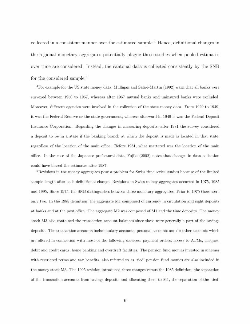
collected in a consistent manner over the estimated sample.4 Hence, definitional changes in

the regional monetary aggregates potentially plague these studies when pooled estimates

over time are considered. Instead, the cantonal data is collected consistently by the SNB

for the considered sample.5

4For example for the US state money data, Mulligan and Sala-i-Martin (1992) warn that all banks were

surveyed between 1950 to 1957, whereas after 1957 mutual banks and uninsured banks were excluded.

Moreover, different agencies were involved in the collection of the state money data. From 1929 to 1949,

it was the Federal Reserve or the state government, whereas afterward in 1949 it was the Federal Deposit

Insurance Corporation. Regarding the changes in measuring deposits, after 1981 the survey considered

a deposit to be in a state if the banking branch at which the deposit is made is located in that state,

regardless of the location of the main office. Before 1981, what mattered was the location of the main

office. In the case of the Japanese prefectural data, Fujiki (2002) notes that changes in data collection

could have biased the estimates after 1987.5Revisions in the money aggregates pose a problem for Swiss time series studies because of the limited

sample length after each definitional change. Revisions in Swiss money aggregates occurred in 1975, 1985

and 1995. Since 1975, the SNB distinguishes between three monetary aggregates. Prior to 1975 there were

only two. In the 1985 definition, the aggregate M1 comprised of currency in circulation and sight deposits

at banks and at the post office. The aggregate M2 was composed of M1 and the time deposits. The money

stock M3 also contained the transaction account balances since these were generally a part of the savings

deposits. The transaction accounts include salary accounts, personal accounts and/or other accounts which

are offered in connection with most of the following services: payment orders, access to ATMs, cheques,

debit and credit cards, home banking and overdraft facilities. The pension fund monies invested in schemes

with restricted terms and tax benefits, also referred to as ‘tied’ pension fund monies are also included in

the money stock M3. The 1995 revision introduced three changes versus the 1985 definition: the separation

of the transaction accounts from savings deposits and allocating them to M1, the separation of the ‘tied’

6

The data on cantonal deposits stem from the following banks: big banks, cantonal

banks, regional savings and loan banks, agricultural banks, and other institutions. Not

included are private banks (Privatbanken), branches of foreign banks, and financial firms

(Finanzgesellschaften). The total of the excluded share represents less than 2% of the

total aggregate. The cantonal domicile of a deposit depends on the address of the bank’s

branch. This is irrespective of the location of the bank’s head office or residence of the

account holder.

Two types of cantonal money stocks are computed. The first cantonal money aggregate,

MC1, is defined as savings plus deposit accounts. Deposit accounts are accounts that have

elements of transactions and savings characteristics. MC1 is similar to the money aggregate

M2, however the cantonal measure does not include currency.6 Figure 1a plots the levels

of MC1 and M2. The correlation of the two series is 0.99 in levels and 0.98 in (ln) first

differences, suggesting that MC1 is a good proxy of M2.

The second cantonal money stock, MC2, is MC1 plus medium-term notes (Kassenobli-

gationen). The medium-term notes, hereafter notes, are issued by individual banks. Notes

are held by households, non profit organizations, local and cantonal governments, and cor-

porations, which can include other banks. Because the maturity of notes lies between one

to seven years, this makes MC2 broader than the money aggregate M3. Money M3 is de-

pension fund monies from the savings deposits, and the allocation of the savings deposits to M2 and the

time deposits to M3.6The 1995 definition of M2 is notes in circulation, sight deposits, transactions accounts plus savings

accounts.

7

fined as M2 plus short-term notes with a maturity of up to five years. Figure 1b plots MC2

and M3. Although the profile of MC2 is slightly smoother than that of M3, the correlation

of the two series remains high for it is 0.98 in levels and 0.54 in (ln) first differences.

It is important to note that while MC1 and MC2 have several attractive properties,

they are not without deficiencies. First, as in the time-series data, Swiss bank accounts

of residents living abroad are included in the cantonal money measure. This would imply

that financial centers such as Zurich would be most affected and that the income elasticities

for that canton would be biased upward under the assumption that financial sophistica-

tion is constant across Switzerland. A second problematic feature of the cantonal money

aggregates is that Swiss residents or Swiss firms may not reside or be located in the same

canton where they hold their account. This would underestimate the income elasticity of

the cantons where the households and firms reside, and overestimate the income elasticity

of those cantons where the bank accounts are held. As will be discussed later, the smallest

cantons are most likely to be affected.

Cantonal Income and Price Indexes

The preferred income measure should include the activity of households and firms, be-

cause our measure of money includes accounts held by both. The Bundesamt fur Statistik

publishes the cantonal income accounts, which are the cantonal version of the GDP statis-

tics. Measures for real and nominal cantonal income are available since 1980. From these

two series, I generate a cantonal price index.

8

Cantonal Interest Rates

The SNB’s Bankwesen publishes cantonal interest rates on savings accounts and notes.

Since banking laws in Switzerland are uniform across cantons, the cantonal rates should not

be segmented because of regulatory decrees. These rates are average rates from cantonal

banks and regional savings banks for the period 1981-1999. Prior to 1981, the cantonal

rates stem only from the cantonal banks. The interest rates of the big banks are not part

of the cantonal averages. No cantonal interest rates are available for 1985.

Figure 2 plots the average (unweighted) cantonal savings and note rate along with their

standard deviations as a measure of interest rate dispersion. Several remarks are offered.

First, the note rate, because of its longer duration, is always higher than the savings rate.

Second, interest rate dispersion is not constant particularly in the latter half of the sample.

Third, the standard deviations do not move together. The level of interest rate dispersion

fell for the savings rate during the 1990s, while it increased for the rate on notes. These

observations offer a different picture to the interest rate assumptions made in Mulligan and

Sala-i-Martin (1992) and Fujiki and Mulligan (1996). Moreover, if financial innovation is

important as the authors of these studies claim, then it is ever more so important that

regional interest rates enter their specification.

Financial Innovation in Switzerland and their Measures

It is difficult to outline all the potential influences of financial innovation on Swiss

money demand over the last two decades. Yet two particular events stand out. The first is

the combined introduction of new liquidity prescriptions and the Swiss Interbank Clearing

9

(SIC) system in 1988. The latter influenced the costs and the technology of the payments

system, whereas the former reduced the reserve requirements for banks. Both of these

changes reduced significantly the demand for central bank giros (reserves) and improved the

financial management of bank assets. These changes in bank operating procedures resulted

in large shifts in the narrow monetary aggregates. The 1988 and the 1989 deviations

between the actual growth rate of the monetary base relative to the SNB’s target were

−7% and −4%. Whether the improvement in cash management and the reduction in

liquidity requirements had repercussions for the broader monetary aggregates has not been

examined in the context of Swiss money demand.

A second form of financial innovation stems from a more concentrated banking system.7

The process, which began in the early 1980s, meant that the Swiss big banks increased their

market power at the expense of regional and cantonal banks. The Swiss big banks are active

nationwide and set reference rates for a range of products. Market segmentation, which

arose from the ability of regional and cantonal banks to exploit their local market power,

was reduced over time.

The gradual concentration of the banking sector has implications for our cross-cantonal

estimates. First, the interest rate elasticity should erode over time. As the degree of

geographical segmentation is eliminated by the greater concentration of the big banks, the

influence of cantonal interest rates should fall over time. Second, a wider range of banking

services offered by the big banks may have generated shifts in portfolio allocation. This

7See Braun et al. (1999) for a detailed discussion concerning the concentration of Swiss banks.

10

could result in a reduction in the use of the traditional accounts defined by broad money,

which should result in a lower income elasticity over time. To capture the gradual change

of financial sophistication across regions and time; the effects of cantonal interest rates,

population density, financial centers, the economic structure of cantons, and ATMs on

money demand will be investigated empirically in sections 3 and 4.

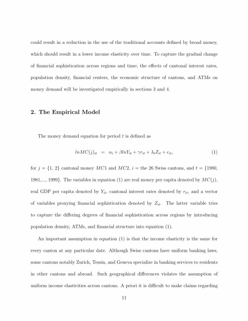
2. The Empirical Model

The money demand equation for period t is defined as

lnMC(j)it = αi + βlnYit + γrit + λtZit + eit, (1)

for j = {1, 2} cantonal money MC1 and MC2, i = the 26 Swiss cantons, and t = {1980,

1981,..., 1999}. The variables in equation (1) are real money per capita denoted by MC(j),

real GDP per capita denoted by Yit, cantonal interest rates denoted by rit, and a vector

of variables proxying financial sophistication denoted by Zit. The latter variable tries

to capture the differing degrees of financial sophistication across regions by introducing

population density, ATMs, and financial structure into equation (1).

An important assumption in equation (1) is that the income elasticity is the same for

every canton at any particular date. Although Swiss cantons have uniform banking laws,

some cantons notably Zurich, Tessin, and Geneva specialize in banking services to residents

in other cantons and abroad. Such geographical differences violates the assumption of

uniform income elasticities across cantons. A priori it is difficult to make claims regarding

11

the direction of the bias. It is possible that the richer cantons, because they have more

professional employees, tend to dominate the banking industry. The data would thus yield

more deposits in a rich canton than its residents would demand. In this case, the income

elasticity estimates would be biased upward. Alternatively, Mulligan and Sala-i-Martin

(1992) argue that richer regional areas can implement more readily the newest technologies,

which allow agents to economize on their cash balances. This effect would bias the income

elasticities downward.

The regression analysis seeks to understand the quantitative importance of this assump-

tion of uniform elasticities. A comparison of income elasticities obtained with and without

cantonal fixed-effects will provide an indicator of the impact of this assumption. In some

specifications, I try to capture the differing degrees of financial sophistication by introduc-

ing the population density or the share of income originating in the agriculture sector as

an explanatory variable. This is meant to capture the possibility that technology diffuses

slowly from urban to rural areas.

3. Empirical Cross-Cantonal Estimates

In this section, I present estimates of income elasticity that deviate sharply from the

time-series estimates. The strategy begins with univariate cross-cantonal estimates of the

income elasticity of money demand. Thereafter, other conditioning variables are added to

test for price homogeneity and the importance of cantonal interest rates. The Appendix

12

provides a review of recent time-series studies that yield coefficient estimates greater than

unity for Swiss income elasticity. It also shows that cross-sectional data are able to replicate

the time-series results when aggregated over cantons.

Table 1 shows the estimates of the income elasticities for MC1 and MC2. The elasticity

estimates are significant at the 5 percent level and are clearly less than one. The estimates

lie between 0.4 and 0.6; consistent with the Baumol-Tobin transactions model with an

income elasticity of 0.5. Figure 3 shows the estimated income elasticities from the univariate

regressions for each year. No clear break after 1988 or downward trend as suggested by

the introduction of SIC payment’s technology and through lower reserve requirements for

banks is detected. Test restrictions that the income elasticity is equal to 0.5 cannot be

rejected. The p-values of this F-test are given by F-test1. When the sample is pooled and

time effects are introduced, the constrained income elasticities are 0.484 for both measures

of cantonal money. The null hypothesis of an income elasticity equal to 0.5 is not rejected

for the pooled estimates.

A possible interpretation of the results in Table 1 is that Swiss money demand is income

elastic, but measurement error gives the appearance of a low elasticity. To test this claim,

an LM test of the Griliches-Hausman estimator versus the Tobin-Baumol point estimate

of 0.5 is conducted for the pooled sample. The p-values of this null hypothesis are 0.41 for

MC1 and 0.27 for MC2, suggesting that measurement error is not an explanation for the

low income elasticity.

The next regression results test for price homogeneity; a property that Swiss time series

13

have difficulty in fulfilling.8 Two tests are conducted. Both find no evidence that this

property is violated. The first test introduces ln(price) in the regressions of Table 1. The

results with ln(price) are given in Table 2. The price variable is insignificant in each

regression and the point estimates of income are close to those of Table 1. F-Test1, which

tests whether the income elasticity is equal to 0.5, continues to have p-values well above

the standard critical values. This first test is unable to reject the null of price homogeneity.

The second test of price homogeneity regresses real money per capita on nominal GDP

per capita and ln(price) and tests whether the coefficient of nominal GDP per capita is

equal to the negative in sign of the coefficient on ln(price). The p-value of this test is

given in the column of F-test2. The p-value is greater than 0.05 in each case except for the

MC1-univariate regression for the year 1980 and the MC1 pooled regression. Overall, the

evidence is strong that price homogeneity is not violated.9

Next, the influence of cantonal interest rates is considered. In previous cross-regional

studies of money demand, this important structural variable has been excluded because of

a lack of data on regional interest rates. Two types of cantonal interest rates are considered:

savings rate and note rate. The savings rate may take on two roles, either as an own rate or

as a short-term opportunity cost measure. It is possible that the former (latter) is constant

over the cross section, yet the opportunity cost (own rate) varies across regions. The rate

for notes is assumed to behave as a long-term measure of capital. The correlation between

8See the long-run money demand studies by Fischer and Peytrignet (1990) and Peytrignet (1996).9The Appendix shows that when aggregating the cantonal data cross sectionally, price homogeneity is

not fulfilled.

14

the note rate and the government bond rate is positive and significant.

The regression results, given in Table 3, show that the coefficients on the savings and

the note rates do not appear stable nor are they significant. The savings rate is significant

only for the year 1986 in the MC1 regression. From this I conclude that cantonal interest

rates do not deviate sufficiently between regions to warrant additional information. For the

remaining regressions in the next section that focus on measures of financial sophistication

across cantons, regional interest rates will not be considered.

4. The Role of Different Levels of Regional Financial Sophistication

The results in the previous section show that the introduction of cantonal prices and

cantonal interest rates do not provide additional information in the standard cross-regional

money demand function. This result together with the observation from Figure 3 that

the income elasticity is stable across time suggests that the potential impact arising from

financial innovation was limited during the last two decades. To test this conjecture,

additional conditional variables that proxy financial sophistication are considered. It begins

by considering the role of population density. Thereafter specific cantons are dropped to test

for the influence of financial centers. Then, the role of financial structure (i.e., openness,

financial size, etc.) within a canton is investigated. Lastly, the influence of ATMs is

considered.

15

Population Density

The population density of a canton represents an attempt to capture differing degrees of

financial sophistication. The argument is that financial sophistication spreads more rapidly

in more densely populated areas because of lower networking costs. Previous studies by

Mulligan and Sala-i-Martin (1992) and Fujiki and Mulligan (1996) show that population

density is an important variable in their cross-regional money demand functions.

The cross-cantonal estimates with population density (PD1) are plotted in Figures 4

and 5. The results show that population density and their higher orders (i.e., PD2, PD3

and denoted respectively as PD2 and PD3) raise the point estimates of income elasticity,

yet the plotted coefficients of PD1, PD2, and PD3 are never significant at the 5-percent

level. From this I conclude that this measure of financial sophistication had little or no

influence on the income elasticity of money demand covering the 1980-1999 period.

Dropping F inancial Centers

An alternative test for financial sophistication is to drop Switzerland’s financial centers

from the sample. This is to control for out-of-canton effects, where residents living abroad or

in neighboring cantons have a preference for holding their bank accounts in Swiss financial

centers. Three cantons with international financial centers are Zurich, Geneva, and Tessin.

The pooled regressions excluding these financial cantons are presented in Table 4. They

show that the coefficients on income remain close to 0.5. The statistic, F-test1, is unable

to reject the null that income elasticity is 0.5. This result is consistent with the view that

the impact of foreign residents holding bank accounts in the financial cantons is marginal

16

for parameter estimates of income elasticity.

As an alternative to financial centers, the exclusion of the smallest cantons with a pop-

ulation less than fifty thousand represents a further check of the influence of bank accounts

held by outside residents. The considered cantons are Glarus, Obwalden, Nidwalden, Uri,

Appenzell AR, and Appenzell IR. Many of the residents from these so-called bedroom can-

tons may hold their bank accounts in neighboring cantons. If this conjecture is correct

in the absence of regional differences in financial sophistication, then the exclusion of bed-

room cantons in the pooled regressions should result in an overestimate of income elasticity.

These regressions yield an income elasticity near 0.6 and the 0.5 restriction given by F-

Test1 is rejected. This somewhat higher point estimate together with the evidence from

the financial cantons does not represent strong evidence of varying levels of financial so-

phistication across the cantons. The evidence, however, suggests that many Swiss residents

may hold bank accounts in cantons outside of their domicile.

Financial Structure

To determine whether a canton’s financial structure has any bearing on income elas-

ticity four measures are considered. The variables are the share of big bank deposits to

total deposits, the ratio of exports to GDP, the ratio of agricultural income to financial

income, and the share of household income to firm income. The first and second measures

represent the degree of big bank concentration and the degree of openness of a canton. The

assumption is that a higher level of big bank concentration and openness in a canton is

associated with a higher level of financial sophistication. This should yield a lower income

17

elasticity. The third ratio between agricultural and financial industry should be negatively

correlated with financial sophistication. The higher is a canton’s share of agriculture with

respect to its financial industry, the lower is the degree of financial sophistication. Again,

this implies that the income elasticity should increase. The fourth ratio considers whether

the canton’s income base is dominated by household or firm income. If it is the latter, then

it is assumed that a canton has a higher level of financial sophistication.

The regressions with various measures of financial structure were estimated using IV

estimation and lagged variables were used as instruments. The evolution of the income

elasticity is plotted in Figures 6 and 7 for the two cantonal monetary aggregates. The

income elasticities display a (slight) negative trend. Overall, the elasticities remain close

to 0.5. Since the standard errors for income elasticity increase when the measures of

financial structure are introduced in the regression, it is still not possible to reject the

coefficient restriction of 0.5 for the individual regressions. The measure of a canton’s

financial structure, however, was always insignificant. From this I conclude that there is

no strong evidence that a canton’s financial structure influences the income elasticities.

The Influence of ATMs

The number of ATMs in a canton provides an alternative measure of a region’s financial

sophistication. A higher level of ATM concentration should be positively correlated with

a higher degree of financial sophistication. The number of ATMs is introduced as an

independent regressor in equation (1). Unfortunately, the location of past ATMs is only

known for the year 1998; a time when the market for ATMs was not yet saturated for

18

double digit growth figures were recorded in the previous years.

Table 5 records the cross-cantonal estimates with the number of ATMs and two concen-

tration measures: ln(ATM/population) and ln(ATM/cantonal area). The ATM results are

insignificant and are consistent with the other proxy measures of financial sophistication.

In each of the cross-cantonal regressions, the ATM variable is insignificant even if the 10

percent critical level is used.

5. Summary and Policy Implications

The paper’s contribution is to present new estimates of income elasticity in light of po-

tential regional differences in financial sophistication. The cross-regional regression analysis

for Switzerland relies on a unique data set that entails cantonal interest rates and cantonal

prices. The ability to account explicitly for an important structural variable that of interest

rates is novel with respect to previous cross-regional money demand studies.

The estimates of income elasticity yield four main empirical results. The first is that

the cross-sectional estimates of income elasticity for broad money range between 0.4 and

0.6. Only in exceptional cases is the coefficient restriction of 0.5 for income elasticity

rejected. The cross-cantonal estimates do not exceed 0.6 even when alternative conditioning

variables are considered in the regression analysis. This estimate for income elasticity

reflects a higher degree of financial sophistication than is borne out from the time-series

estimates. A second empirical result is that measures capturing differing levels of financial

19

technology across regions have no distinguishable impact on the point estimates for income

elasticity between 1980 and 1999. This result is underscored by the insignificance of the

cantonal interest rates. A related and third result is that the cross-cantonal estimates for

income elasticity are stable not only across regions but also across time. This result re-

enforces the view that financial innovation did not significantly influence income elasticity

for broad money. The fourth result is that the cross-cantonal estimates for Switzerland

are at odds with recent cross-regional money demand studies for other countries. Studies

by Fujiki and Mulligan (1996) and Mulligan and Sala-i-Martin (1992) find that income

elasticity is greater than one and the population density, which acts as a proxy for financial

sophistication, is statistically significant in Japanese and U.S. money demand equations.

Neither of these properties hold for Switzerland. A tentative conclusion is that country

size matters. Financial sophistication across regions affects large countries more than small

countries, even if they are culturally and linguistically diverse as Switzerland.

Several policy conclusions emerge from the above mentioned results. The first concerns

identifying an acceptable level of money growth. If per capita output growth proceeds at

2 percent, an overestimate of the income elasticity by 0.5 or 1.0 would result in a higher

inflation rate of 1% to 2% instead of the intended level. Policy recommendations based

on velocity indicators or time-series estimates for money demand will tolerate a higher

level of money growth that is consistent with price stability than those stemming from the

cross-cantonal estimates.

The result that the estimates of income elasticity are stable across time and regions offers

20

renewed confidence for money as an important indicator for monetary policy. Although

the empirical results do not demonstrate that Swiss money demand is stable, they are

consistent with the view that unstable estimates of income elasticity may be a statistical

property arising from time-series data.

A further policy implication arising from the cross-sectional estimates is that they are

consistent with traditional transactions theory of money demand. This redefines the re-

search agenda for Swiss money demand. If the new cross-cantonal estimates are accepted,

it is no longer necessary to rely on conjectures of family decomposition (see Mulligan and

Sala-i-Martin, 1992), the use of the correct scale variable (Baltensperger et al. 2001), or

backward bending labor supply curves (Mankiw, 1992) to justify income elasticities greater

than one. While such hypotheses enjoy considerable appeal among many economists, the

support for such explanations rests on weak empirical foundations in Switzerland.

21

References

Adao, B., Mata, J., 1999, Money Demand and Scale Economies: Evidence from a Panel ofFirms, manuscript.

Baltensperger, E., Jordan, T. J., Savioz, M. R. 2001, The Demand for M3 and InflationForecasts: An Empirical Analysis for Switzerland, Weltwirtschaftliches Archiv 137, 244-72.

Belongia, M. T. 1988, Stability of Swiss Money Demand: Evidence for 1982-1987, Geld,Wahrung und Konjunktur, SNB Quartalsheft 6, 68-74.

Boswijk, J. P. Urbain, J.P., 1997, Lagrange-Multiplier Tests for Weak Exogeneity: A Syn-thesis, Econometric Review 16, 21-38.

Bover, O., Watson, N., 2001, Are There Economies of Scale in the Demand for Money byFirms? Some Panel Estimates, CEPR Working Paper No. 2818.

Braun, C., Egli, D., Fischer, A. M., Rime, B., Walter, C., 1999, The Restructuring of theSwiss Banking System, in The Monetary and Regulatory Implications of Changes inthe Banking Industry, Bank for International Settlements, 70-96.

Fischer, A. M., Peytrignet, M., 1991, The Lucas Critique in Light of Swiss Monetary Policy,Oxford Bulletin of Economics and Statistics 53, 481-493.

Fischer, A. M., Peytrignet, M., 1990, Are Larger Monetary Aggregates Interesting? SomeExploratory Evidence for Switzerland Using Feedback Models, Schweizerische Zeitschriftfur Volkswirtschaft und Statistik 126, 505-20.

Fujiki, H., 2002, Money Demand near Zero Interest Rate: Evidence from Regional Data,Monetary and Economic Studies 20, 25-41.

Fujiki, H., Hsiao, C., Shen, Y., 2002, Is There a Stable Money Demand Function under theLow Interest Rate Policy? A Panel Data Analysis, Monetary and Economic Studies 20,1-23.

Fujiki, H., Mulligan, C. B., 1996, A Structural Analysis of Money Demand: Cross-SectionalEvidence from Japan, Monetary and Economic Studies 14, 53-78.

Jordan, T. J., Peytrignet, M., Rich, G., 2000, The Role of M3 in the Policy Analysis ofthe Swiss National Bank, paper presented as the Central Bank Workshop on MonetaryAnalysis, Frankfurt November 20 and 21, 2000.

Kohli, U., 1984, La demande de Monnaie en Suisse, Geld, Wahrung und Konjunktur SNBQuartalsheft 2, 251-278.

Kristen-Gerlach, P., 2000, The Demand for Money in Switzerland 1936-1995, SchweizerischeZeitschrift fur Volkswirtschaft und Statistik 137, 535-54.

Lucas, R. E., 2000, Inflation and Welfare, Econometrica 68, 247-74.Mankiw, N. G., 1992, Comments and Discussion, Brooking Papers on Economic Activity

2, 330-334.Mulligan, C. B., 1997a, Scale Economies, the Value of Time, and the Demand for Money:

Longitudinal Evidence from Firms, Journal of Political Economy 105, 1061-1079.Mulligan, C. B., 1997b, The Demand for Money by Firms: Some Additional Empirical

Results, Discussion Paper 125, Federal Reserve Bank of Minneapolis.Mulligan, C. B., Sala-i-Martin, X., 1992, U.S. Money Demand: Surprising Cross-sectional

Estimates, Brooking Papers on Economic Activity 2, 285-329.Peytrignet, M., 1996, Stabilite econometrique des agregats monetaries suisses, Geld, Wahrung

und Konjunktur SNB Quartalsheft 15, 251-278.Peytrignet, M., Stahel, C., 1998, Stability of Money Demand in Switzerland, Empirical

Economics 23, 437-454.

22

Reynard, S., 2004, Financial Market Participation and the Apparent Instability of MoneyDemand, Journal of Monetary Economics 51, 1297-1317.

Slok, T., 2002, Money Demand in Mongolia: A Panel Data Analysis, IMF Staff Papers 49,128-135.

23

Appendix: Time Series Results with Aggregate Cross-Cantonal Data

A stylized fact of Swiss time series studies of broad money demand is that their (long-run) income elasticities are above unity. Table A1 presents an overview of the empiricalestimates for the monetary aggregates M2 and M3. With the exception of Belongia (1988)the point estimates for income elasticity lie between 1 and 2. Several studies have suggestedthat estimates of income elasticity are biased upward through the use of the incorrect scalevariable for broad money demand. Kristen-Gerlach (2001) and Baltensperger et al. (2001)argue that wealth rather than GDP income is the preferred variable. Others such asPeytrignet (1996) suggest that problems of a high income elasticity stem from improperprice indices. The latter study shows that price homogeneity is not fulfilled in standardcointegration models and that once this restriction is imposed income elasticity falls to anacceptable level near unity.

Table A2 presents the estimated the long-run income elasticity using the cross-cantonaldata aggregated across cantons. The OLS equation should be treated as the static equationof the cointegration relation. Tests for cointegration were not performed because of thelow number of observations. The low R2s for many the regressions suggests that thecointegration assumption may be violated. The intention however is to show that thecantonal data are able to replicate the time series estimates for income elasticity given inTable A1.

The parameter estimates on income for the full sample lie between 1.08 and 1.5 forMC1 and are near unity for MC2. These estimates are consistent with those studies thatcover the same or nearly the same sample period. Peytrignet (1996) and Peytrignet andStahel (1998) obtain estimates between 1 and 1.5 for the monetary aggregate M2 andBaltensperger et al. (2001) present estimates of 1 for the monetary aggregate M3. Table A2also shows that income elasticity is sensitive to sample length and to the variables includedin the static equation. This result is consistent with the time series results presented inPeytrignet (1996). A further result is that price homogeneity is strongly rejected: a featurenot fulfilled by time series studies.

24

25

26

27

28

29

30

31

Table 1: Cross-Cantonal Regression Results for Income Elasticity

Dep. Variable: MC1 Sample Y Standard Dev. R2 [F-Test1]

1980 0.408* (0.189) 0.143 [0.626]

1985 0.479* (0.113) 0.330 [0.854]

1990 0.467* (0.131) 0.347 [0.804]

1995 0.477* (0.141) 0.343 [0.871]

1999 0.587* (0.203) 0.154 [0.667]

1980-1999 0.484* (0.033) 0.516 [0.546]

Dep. V ariable : MC2

1980 0.532* (0.192) 0.230 [0.868]

1985 0.531* (0.147) 0.354 [0.831]

1990 0.475* (0.156) 0.300 [0.874]

1995 0.404* (0.151) 0.235 [0.527]

1999 0.521* (0.205) 0.113 [0.917]

1980-1999 0.484* (0.037) 0.363 [0.674]

Notes: Regressions include a constant or time effect, which are not shown. Robust standard

errors are given in parentheses. Significance at the 5% level is denoted by *. F-test1, given

in brackets, is the p-value of an F-test for the null hypothesis that the income elasticity = 0.5.

32

Table 2: Income Elasticity and Price Homogeneity

MC1 Sample Y Price R2 [F-test1] [F-test2]

1980 0.411* -1.696 0.190 [0.630] [0.019]

(0.183) (2.350)

1985 0.483* -4.735 0.361 [0.894] [0.255]

(0.13) (4.197)

1990 0.471* -0.215 0.321 [0.836] [0.704]

(0.137) (0.566)

1995 0.510* -0.976 0.325 [0.937] [0.591]

(0.126) (1.800)

1999 0.573* 0.553 0.120 [0.703] [0.726]

(0.192) (1.647)

1980-1999 0.489* -0.806 0.519 [0.734] [0.007]

(0.032) (0.586)

Note: Table continues on the next page.

33

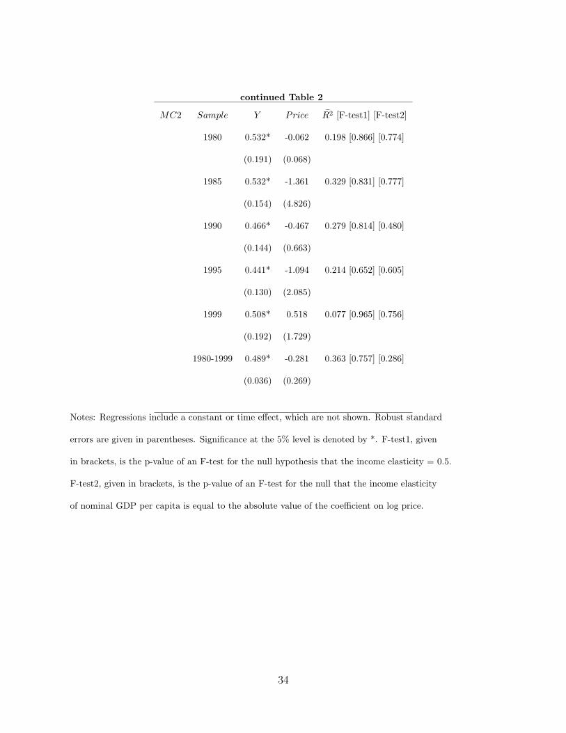
continued Table 2

MC2 Sample Y Price R2 [F-test1] [F-test2]

1980 0.532* -0.062 0.198 [0.866] [0.774]

(0.191) (0.068)

1985 0.532* -1.361 0.329 [0.831] [0.777]

(0.154) (4.826)

1990 0.466* -0.467 0.279 [0.814] [0.480]

(0.144) (0.663)

1995 0.441* -1.094 0.214 [0.652] [0.605]

(0.130) (2.085)

1999 0.508* 0.518 0.077 [0.965] [0.756]

(0.192) (1.729)

1980-1999 0.489* -0.281 0.363 [0.757] [0.286]

(0.036) (0.269)

Notes: Regressions include a constant or time effect, which are not shown. Robust standard

errors are given in parentheses. Significance at the 5% level is denoted by *. F-test1, given

in brackets, is the p-value of an F-test for the null hypothesis that the income elasticity = 0.5.

F-test2, given in brackets, is the p-value of an F-test for the null that the income elasticity

of nominal GDP per capita is equal to the absolute value of the coefficient on log price.

34

Table 3: Estimates for Income and Interest-Rate Elasticity

MC1 1980 1986 1990 1995 1999 1980-1999

Y 0.420* (0.189) 0.490* (0.098) 0.475* (0.120) 0.522* (0.141) 0.467* (0.155) 0.480* (0.031)

S-Rate -0.073 (0.255) 1.545* (0.771) 0.227 (0.418) 0.875 (0.518) -0.926 (1.186) -0.049 (0.346)

R2 [F-test1] 0.110 [0.670] 0.365 [0.918] 0.326 [0.835] 0.375 [0.876] 0.191 [0.830] 0.516 [0.521]

Y 0.374* (0.188) 0.475* (0.144) 0.472* (0.133) 0.437* (0.146) 0.412* (0.194) 0.476* (0.034)

N -Rate -0.408 (1.703) 0.750 (4.886) 0.272 (1.169) -1.170 (0.985) -0.414 (0.570) 0.280 (0.327)

R2 [F-test1] 0.08 [0.506] 0.270 [0.862] 0.320 [0.834] 0.353 [0.664] 0.280 [0.652] 0.564 [0.484]

MC2

Y 0.563* (0.189) 0.542* (0.150) 0.479* (0.151) 0.462* (0.146) 0.414* (0.160) 0.480* (0.036)

S-Rate -0.199 (0.244) 1.309 (0.722) 0.104 (0.444) 1.123* (0.524) -0.824 (1.204) -0.067 (0.302)

R2 [F-test1] 0.208 [0.737] 0.355 [0.778] 0.270 [0.889] 0.301 [0.8140] 0.280 [0.652] 0.362 [0.576]

Y 0.563* (0.193) 0.608* (0.165) 0.512* (0.146) 0.384* (0.153) 0.336 (0.200) 0.483* (0.038)

N -Rate 0.316 (1.499) 3.773 (4.370) 2.175 (1.265) -0.595 (1.043) -0.591 (0.673) 0.428 (0.362)

R2 [F-test1] 0.213 [0.746] 0.325 [0.515] 0.347 [0.936] 0.212 [0.450] 0.184 [0.412] 0.390 [0.647]

Notes: Regressions include a constant or time effect, which are not shown. Robust standard

errors are given in parentheses. Significance at the 5% level is denoted by *. F-test1, given

in brackets, is the p-value of an F-test for the null hypothesis that the income elasticity = 0.5.

35

Table 4: Dropping Financial Centers from the Regressions (1980-1999)

MC1 Dropped from Sample Income Elasticity Standard Dev. R2 [F-test1]

Zurich 0.466* (0.036) 0.496 [0.351]

Geneva 0.506* (0.034) 0.523 [0.861]

Tessin 0.471* (0.034) 0.528 [0.394]

Bedroom Cantons 0.580* (0.017) 0.700 [0.000]

MC2

Zurich 0.452* (0.041) 0.337 [0.240]

Geneva 0.541* (0.034) 0.400 [0.226]

Tessin 0.480* (0.037) 0.363 [0.600]

Bedroom Cantons 0.621* (0.022) 0.523 [0.000]

Notes: Regressions include a constant or time effect, which are not shown. Robust standard

errors are given in parentheses. Significance at the 5% level is denoted by *. F-test1, given

in brackets, is the p-value of an F-test for the null hypothesis that the income elasticity = 0.5.

36

Table 5: The Influence of ATMs in 1998

MC1

Y 0.605* (0.242) 0.639* (0.270) 0.596* (0.247) 0862* (0.355)

ATM -0.019 (0.063)

log(ATM/POP ) 0.042 (0.116)

log(ATM/Area) -0.078 (0.078)

R2 0.173 0.142 0.143 0.173

MC2

Y 0.549* (0.252) 0.600* (0.281) 0.542* (0.258) 0808* (0.378)

ATM -0.029 (0.066)

log(ATM/POP ) 0.036 (0.121)

log(ATM/Area) -0.079 (0.082)

R2 0.131 0.100 0.096 0.127

Notes: The number of ATMs in a canton are denoted by ATM . Regressions include a constant (not shown).

Robust standard errors are given in parentheses. Significance at the 5% level is denoted by *.

37

Table A1: Long-Run Income Elasticity for Broad Money Demand

Empirical Study Point Est. for Income Sample Money Agg.

Belongia (1988) 1.25 1968:1-1986:4 M2

Boswijk and Urbain (1997) 1.38 1973:1 1989:4 M2

Fischer and Peytrignet (1991) 1.05 1973:1 -1989:4 M2

Kohli (1984) 1.07 1959-1983 M2

Peytrignet (1996) 1.06-1.51 1977:1-1994:4 M2

Peytrignet and Stahel (1998) 1.04 1977:1-1997:1 M2

Baltensperger, Jordan, Savioz (2001) 1.05 1978:1-1999:2 M3

Belongia (1988) 0.70 1968:1-1986:4 M3

Fischer and Peytrignet (1990) 1.55 1967:3-1989:4 M3

Jordan, Peytrignet, Rich (2000) 1.3 1977:1-1986:4 M3

Kohli (1984) 1.24 1959-1983 M3

Kristen-Gerlach (2001) 1.26 1936-1995 M3

Peytrignet (1996) 1.83-2.0 1977:1-1994:4 M3

Peytrignet and Stahel (1998) 1.69 1977:1-1997:1 M3

38

Table A2: Time-Series Estimates of Long-Run Income Elasticity

Dep. V ariable: MC1 1980-1999 1980-1995 1986-1999

Income 1.461* (0.553) 0.446* (0.445) 0.370* (1.296)

R2 0.206 -0.007 -0.070

Inc. Elasticity = 1 0.404 0.172 0.627

Homogeneity 0.000 0.000 0.000

Income 1.080* (0.327) 1.504* (0.363) -0.497 (0.460)

Savings Rate -0.337* (0.047) -0.505* (0.083) -0.359* (0.028)

R2 0.781 0.541 0.894

Inc. Elasticity = 1 0.800 0.165 0.001

Homogeneity 0.000 0.000 0.000

Income 1.495* (0.400) 0.879 (0.451) 0.184 (0.852)

Note rate -0.741* (0.165) -0.442 (0.242) -0.772* (0.143)

R2 0.532 0.085 0.450

Inc. Elasticity = 1 0.216 0.789 0.337

Homogeneity 0.000 0.000 0.000

Notes: Table continues on the next page.

39

Continued Table A2

Dep. V ariable : MC2 1980-1999 1980-1995 1986-1999

Income 1.022* (0.238) 1.059* (0.257) -0.490 (0.376)

R2 0.414 0.404 0.041

Inc. Elasticity = 1 0.927 0.820 0.000

Homogeneity 0.025 0.314 0.725

Income 0.995* (0.241) 1.629* (0.311) -0.587 (0.387)

Savings Rate -0.024 (0.038) -0.272* (0.083) -0.040* (0.021)

R2 0.392 0.579 0.120

Inc. Elasticity = 1 0.982 0.000 0.000

Homogeneity 0.282 0.551 0.620

Income 1.026* (0.253) 1.494* (0.324) -0.521 (0.403)

Note rate -0.097 (0.121) -0.444* (0.146) -0.127* (0.069)

R2 0.403 0.574 0.161

Inc. Elasticity = 1 0.917 0.127 0.000

Homogeneity 0.014 0.000 0.597

Notes: A constant (not shown in Table 2) is included in the regressions. Consistent heteroscedastic

standard errors of the coefficients are in parentheses. Significance at the 5% level is denoted by *. Income is

real GDP per capita, Savings rate is the average cantonal savings rate. Note rate is the average cantonal rate for

notes. Inc. Elasticity is the p-value of an F-test under the null hypothesis that the income elasticity is unity.

Homogeneity is the p-value of an F-test under the null that log price is insignificant in the same regression.

40

Swiss National Bank Working Papers published since 2004: 2004-1 Samuel Reynard: Financial Market Participation and the Apparent Instability of

Money Demand 2004-2 Urs W. Birchler and Diana Hancock: What Does the Yield on Subordinated Bank Debt Measure? 2005-1 Hasan Bakhshi, Hashmat Khan and Barbara Rudolf: The Phillips curve under state-dependent pricing 2005-2 Andreas M. Fischer: On the Inadequacy of Newswire Reports for Empirical Research

on Foreign Exchange Interventions 2006-1 Andreas M. Fischer: Measuring Income Elasticity for Swiss Money Demand: What

do the Cantons say about Financial Innovation?

Swiss National Bank Working Papers are also available at www.snb.ch, section Publications/ResearchSubscriptions or individual issues can be ordered at Swiss National Bank, Fraumünsterstrasse 8, CH-8022 Zurich,fax +41 44 631 81 14, E-mail library@snb.ch