ANDREJS BESSONOVS OĻEGS KRASNOPJOROVS 1 / 2020

1 / 2020WORKING PAPER

ISBN 978-9934-578-22-9

ANDREJS BESSONOVSOĻEGS KRASNOPJOROVS

SHORT-TERM INFLATION PROJECTIONS MODEL AND ITS ASSESSMENT IN LATVIA

© Latvijas Banka, 2020

This source is to be indicated when reproduced.

Latvijas BankaK. Valdemāra iela 2A, Riga, LV-1050Tel.: +371 67022300 [email protected]

http://www.bank.lv https://www.macroeconomics.lv

S H O R T - T E R M I N F L A T I O N P R O J E C T I O N S M O D E L A N D I T S A S S E S S M E N T I N L A T V I A

2

CONTENTS

CONTENTS 2 SUMMARY 3 1. INTRODUCTION 4 2. LITERATURE REVIEW 5 3. DATA AND METHODS 6 3.1 Data 6 3.2 Modelling approach 6 4. SHORT-TERM INFLATION PROJECTIONS MODEL 7 4.1 Unprocessed food prices 9 4.2 Processed food prices 10 4.3 Energy prices 12 4.4 Non-energy industrial goods prices 15 4.5 Services prices 16 5. THE IMPACT OF DOMESTIC AND FOREIGN SHOCKS 17 5.1 Pass-through of global food commodity prices to consumer prices 18 5.2 Pass-through of crude oil prices to consumer prices 20 5.3 Pass-through of wages to consumer prices 23 6. FORECAST EVALUATION 25 7. CONCLUSIONS 29 APPENDIX 30 BIBLIOGRAPHY 53

ABBREVIATIONS

ADF test – Augmented Dickey–Fuller test ARDL – autoregressive distributed lag BMPE – Broad Macroeconomic Projection Exercise CEC – conditional error correction CPI – Consumer Price Index CSB – Central Statistical Bureau of Latvia DG AGRI – Directorate-General for Agriculture and Rural Development of the EC DM test – Diebold–Mariano test EC – European Commission ECB – European Central Bank ESCB – European System of Central Banks EU – European Union EUR – euro Eurostat – Statistical Bureau of the EU HICP – Harmonised Index of Consumer Prices LV – Latvia NEER – nominal effective exchange rate n.e.c. – not elsewhere classified NEIG – non-energy industrial goods NIPE – Narrow Inflation Projection Exercise pp – percentage point PUC – Public Utilities Commission RMSFE – root mean squared forecast error STIP model – Short-Term Inflation Projections model of Latvijas Banka US – United States of America USD – US dollar VAT – value added tax


3

SUMMARY

This paper develops a Short-Term Inflation Projections (STIP) model, which captures cointegrated relationships between highly disaggregated consumer prices and their determinants. We document a significant pass-through of domestic labour costs, crude oil and global food commodity prices to consumer prices in Latvia. We also assess the model's forecast accuracy of Latvia's inflation during 2014–2018 and find that the STIP model statistically significantly outperforms a naïve benchmark model in real time.

Keywords: inflation forecasting, autoregressive distributed lag model, pass-through, oil prices, food commodity prices, labour costs

JEL codes: C32, C51, C52, C53, E31

The authors would like to thank an anonymous external reviewer, as well as Andrejs Zlobins and Boriss Siliverstovs (Latvijas Banka) for their comments and suggestions. The views expressed in this paper are exclusively those of its authors, who are employees of Latvijas Banka's Monetary Policy Department, and do not necessarily reflect the official position of Latvijas Banka. The authors assume sole responsibility for any errors and omissions. E-mail: [email protected], [email protected].


4

1. INTRODUCTION

Price stability is the ultimate goal of monetary policy in the euro area. Monetary policy transmission implies that not only the current inflation of consumer prices but also the projected one is important for making monetary policy decisions. In practice, each central bank in the euro area develops short-term inflation projections for the respective country which are then aggregated to euro area inflation projections, providing inputs to the ECB's monetary policy decisions.

Against this backdrop, we build a model, which projects inflation developments over a short-term horizon (12 months) in Latvia, and call it the STIP model. It plays an important role in assessing short-term inflation projections in the context of BMPEs/NIPEs, which are procedural frameworks of the Eurosystem/ECB macroeconomic projections1. In the Eurosystem, disaggregated short-term inflation projections serve as a starting-point for the medium to longer-term inflation projections (ECB (2010)).

In particular, the NIPE requires to provide inflation projections that are disaggregated in specific components. This approach is rationalised by the fact that individual inflation components are affected by different factors. These factors naturally are driven either by developments in domestic or foreign markets. For instance, energy consumer prices are heavily dependent on developments in global crude oil markets, whereas services consumer prices are mainly affected by economic developments in the domestic market. Hence, both energy and services prices have different driving forces, and consequently they should be modelled separately. In this paper we follow the bottom-up modelling strategy approach, i.e. we model and forecast 34 components of consumer price inflation and aggregate them to headline inflation. The extent of disaggregation in our model is quite high compared to the literature, thereby it allows us to take into account all available and useful information, which might point to price changes in the future. To assess the link between prices and their determinants, we employ the ARDL modelling approach by Pesaran and Shin (1998). The advantage of this approach lies in its ability to estimate cointegrating relationships. This allows us to capture rich dynamics of the modelling approach, but cointegration ensures tractability between consumer prices and their determinants.

We conclude that the STIP model withstands well two main exercises. First, it captures a pass-through of domestic labour costs, global food commodity prices and crude oil prices to consumer prices in Latvia. In this paper we discuss both direct and indirect effects of domestic and foreign shocks on consumer prices in Latvia. Second, the STIP model forecasts accurately inflation and its components over 12 months ahead. We assess the model's out-of-sample forecast accuracy and find that the STIP model statistically significantly outperforms a naïve benchmark model in real time.

The structure of the paper is the following. Section 2 reviews the literature. Section 3 describes the data and methods. Section 4 presents estimation results. Section 5 discusses the impact of the main domestic and foreign shocks on consumer prices in Latvia. Section 6 assesses the model's out-of-sample forecast performance, while Section 7 concludes.

1 The BMPE is a projection exercise conducted by the Eurosystem twice per year, while the NIPE is an inflation projection exercise concomitant to the BMPE, but conducted four times per year over a shorter forecast horizon to monitor inflation developments. For details, see ECB (2016).


5

2. LITERATURE REVIEW

The bottom-up modelling approach is well studied in the literature on theoretical and empirical grounds, which, in particular, examines whether the disaggregated approach is more accurate compared to the aggregated one. The efficiency of disaggregated approach is highlighted by Lütkepohl (1984a; 1984b; 1987), assuming that data generation processes are known or correctly estimated. See also Hubrich (2005) and Hendry and Hubrich (2011) for excellent review of the literature on the merits of disaggregated approach. In empirical studies on consumer prices, the disaggregated approach is also proved more accurate than the aggregated one, e.g. Duarte and Rua (2007) for Portugal, Moser et al. (2007) for Austria, Álvarez and Sánchez (2017) for Spain, den Reijer and Vlaar (2006) for the Netherlands, Bruneau et al. (2007) for France, Huwiler and Kaufmann (2013) for Switzerland, Pufnik and Kunovac (2006) for Croatia, Aron and Muellbauer (2012) for South Africa, Espasa et al. (2002a) for the US, Benalal et al. (2004) and Marcellino et al. (2003) for the euro area.

The degree of disaggregation is usually somewhat ad hoc in the literature. As a rule of thumb, authors single out the most heterogeneous or volatile series, which apparently are driven by specific explanatory factors. As a matter of fact, central banks conventionally distinguish five special aggregates, separating the most volatile ones: unprocessed food, processed food, energy, NEIG and services. This approach is followed by Espasa et al. (2002b), Fritzer et al. (2002), den Reijer and Vlaar (2006), Duarte and Rua (2007), Bermingham and D'Agostino (2014) and Álvarez and Sánchez (2017). Several papers disaggregate the consumer price index even further, e.g. Aron and Muellbauer (2012) break down headline consumer prices in 10 components, Stakėnas (2015) – in 21 components, Bermingham and D'Agostino (2014) – in 32 components, Duarte and Rua (2007) – in 59 components, Huwiler and Kaufmann (2013) – in 182 components. In this paper we do not aim at studying the optimal degree of disaggregation but suggest our own level of disaggregation which is largely based on expert judgement and remains fixed throughout the paper.

The literature on inflation forecasting uses various econometric techniques. Predominantly, authors exploit univariate and multivariate techniques, such as ARIMA (Marcellino et al. (2006), Huwiler and Kaufmann (2013)), vector autoregressions (Banbura et al. (2010), Giannone et al. (2014)) and dynamic factor models (Stock and Watson (1999; 2002), Boivin and Ng (2005)), which are characterised by capturing rich dynamics among the variables. In this paper we employ cointegration relationships among consumer prices and their determinants to forecast inflation. Aron and Muellbauer (2012) point out that the empirical literature on the use of long-term relationships in the inflation forecasting is quite scarce, and they tend to by-pass it. However, one might find stable cointegrated relationships between consumer prices and other variables, which may improve inflation forecasts, introducing correction towards equilibrium.

Nonetheless, the amount of literature using cointegration in forecasting inflation is growing. Espasa et al. (2002b) and Espasa and Albacete (2007) forecast inflation in the euro area, and Espasa et al. (2002a) forecast inflation in the US by using cointegration relations. Peach et al. (2004) employ vector error correction models in forecasting inflation in the US. Aron and Muellbauer (2012; 2013) employ cointegration analysis when constructing inflation forecasting models for South Africa and the US respectively. A recent attempt to use cointegration relations in


6

forecasting inflation is made in Stakėnas (2015) for Lithuania. This literature finds out that isolating the equilibrating relationships contribute to greater accuracy of inflation forecasts relative to the benchmark models.

3. DATA AND METHODS

3.1 Data

We use 95 individual HICP from Eurostat and the CSB over the period from 2005 to 2018. The individual indices are aggregated to obtain special aggregates (like unprocessed meat or NEIG) we use in modelling according to ECOICOP5 classification. After the methodological changeover from COICOP4 to ECOICOP5 at the beginning of 2019, several indices (predominantly, individual items of food prices) are publicly available only from 2015. Eurostat does not backcast them to 2005. Therefore, these indices were obtained from the CSB2.

We also use various data as determinants of consumer prices. To explain car fuel prices, we use crude oil prices (Bloomberg, Brent mark, daily data), refined petrol and diesel prices (Bloomberg and Reuters, daily) and retail car fuel prices before and after taxes (the weekly Oil Bulletin of the EC), as well as the EUR–USD exchange rate obtained from the ECB (Statistical Data Warehouse).

Global food commodity prices, which determine consumer prices of food components, are represented by European farm-gate prices and other agricultural prices of cereals, dairy and meat and are published by the DG AGRI of the EC. International food commodity prices of sugar and coffee are used to explain the respective consumer prices (Bloomberg). We employ Nasdaq salmon spot prices as a proxy for international fish prices.

Other domestic explanatory variables are the average wage rate from firms' surveys (CSB) as a measure of domestic labour costs, the hotel occupancy rate (CSB) to control for demand pressures in accommodation services and the internet usage (CSB) to explain communication prices.

Ultimately, explanatory variables should be attributed to the future path over the forecast horizon in order to make inflation projections. Almost all foreign variables follow the assumptions provided by the ECB during NIPE forecast rounds, i.e. crude oil prices, global food commodity prices and the exchange rate. Whereas, the projections of labour costs, salmon prices, the hotel occupancy rate and internet usage are elaborated by Latvijas Banka internally. All consumer prices (except the administered prices and energy prices) are seasonally adjusted by X-12-ARIMA with default settings.

3.2 Modelling approach

We employ the ARDL modelling approach following Pesaran and Shin (1998) and Pesaran et al. (2001) to empirically assess long-run level relationships between consumer prices and their determinants. The ARDL approach enables us to test for a level relationship irrespective whether the regressors are of the order I(0) or I(1).

2 We are indebted to Natalja Dubkova and Dāvis Liberts from the CSB for their benevolence providing us with the required backcasted data.


7

The general representation of ARDL is the following:

𝑦𝑦𝑡𝑡 = 𝑎𝑎0 + 𝑎𝑎1𝑡𝑡 + ∑ 𝜓𝜓𝑖𝑖𝑦𝑦𝑡𝑡−𝑖𝑖𝑝𝑝𝑖𝑖=1 + ∑ ∑ 𝛽𝛽𝑗𝑗,𝑙𝑙𝑗𝑗𝑥𝑥𝑗𝑗,𝑡𝑡−𝑙𝑙𝑗𝑗

𝑞𝑞𝑗𝑗𝑙𝑙𝑗𝑗=0

𝑘𝑘𝑗𝑗=1 + 𝜖𝜖𝑡𝑡 (1)

where 𝜖𝜖𝑡𝑡~𝑖𝑖. 𝑖𝑖.𝑑𝑑.𝑁𝑁(0,𝜎𝜎2), 𝑎𝑎0 is a constant, 𝑡𝑡 is a trend; 𝑎𝑎1, 𝜓𝜓𝑖𝑖,𝛽𝛽𝑗𝑗,𝑙𝑙𝑗𝑗 are respectively the coefficients addressing the linear trend, lags of dependent variable 𝑦𝑦𝑡𝑡, and lags of independent variables 𝑥𝑥𝑗𝑗,𝑡𝑡, for 𝑗𝑗 = 1, … ,𝑘𝑘; and 𝑞𝑞𝑗𝑗 is the number of lags for the independent variable 𝑗𝑗.

Pesaran et al. (2001) show that the vector autoregression framework could be reduced to the CEC form under certain assumptions. Moreover, they show that there is a one-to-one correspondence between the CEC model and the ARDL model presented in (1). Hence, the ARDL model representation could be transformed to the following CEC form:

∆𝑦𝑦𝑡𝑡 = 𝑎𝑎0 + 𝑎𝑎1𝑡𝑡 + 𝑏𝑏0𝑦𝑦𝑡𝑡−1 + ∑ 𝑏𝑏𝑗𝑗𝑥𝑥𝑗𝑗,𝑡𝑡−1𝑘𝑘𝑗𝑗=1 + ∑ 𝑐𝑐0,𝑖𝑖∆𝑦𝑦𝑡𝑡−𝑖𝑖

𝑝𝑝−1𝑖𝑖=1 +

+∑ ∑ 𝑐𝑐𝑗𝑗,𝑙𝑙𝑗𝑗∆𝑥𝑥𝑗𝑗,𝑡𝑡−𝑙𝑙𝑗𝑗𝑞𝑞𝑗𝑗−1𝑙𝑙𝑗𝑗=1

𝑘𝑘𝑗𝑗=1 + ∑ 𝑑𝑑𝑗𝑗∆𝑥𝑥𝑗𝑗,𝑡𝑡

𝑘𝑘𝑗𝑗=1 + 𝜖𝜖𝑡𝑡 (2)

where the third and fourth terms of equation (2), i.e. the lagged terms of dependent variable 𝑦𝑦𝑡𝑡−1 and regressors 𝑥𝑥𝑗𝑗,𝑡𝑡−1, represent a cointegration relationship. Pesaran et al. (2001) propose a bounds test for cointegration as a test on significance of parameters in the cointegration relationship. In fact, the null hypothesis tests whether coefficients 𝑏𝑏0 = 𝑏𝑏𝑗𝑗 = 0, for all 𝑗𝑗, mean that there is no long-run relationship between 𝑦𝑦𝑡𝑡 and 𝑥𝑥𝑡𝑡. Alternatively, if the coefficients are not zeros, we reject the null and conclude that there is a cointegration relationship. The proposed test is a standard F-test, but since asymptotic distributions of this statistic are non-standard under the null, Pesaran et al. (2001) provide critical values. Pesaran et al. (2001) also distinguish five different specifications of the CEC model depending on whether the constant and trend integrate (mutually or separately) into the error correction term. In our model specifications we additionally report whether the trend or constant are included into the cointegration relationship.

The methodology mainly requires that the order of the variables integrated is not greater than I(1), which is indeed true for most economic variables, and ARDL equations should not exhibit serial correlation to ensure cointegration among the variables. We test for the integration order of variables using ADF test statistics, and all of them are not greater than I(1), meaning that variables are 1st difference stationary (see Table A1). The cointegration results between consumer prices and their determinants are tested using the Pesaran–Shin–Smith bounds test and reported in Table A2. The null hypothesis of no serial correlation is tested using the Breusch–Godfrey LM test and is not rejected in all equations (see Table A3). Heteroskedasticity is tested using the Breusch–Pagan–Godfrey test. The null hypothesis is not rejected in a large number of equations, meaning that the errors are homoskedastic. But in cases where heteroskedasticity is present, we use Newey–West adjusted standard errors (see Table A3). Other statistics of the estimated equations are reported in Table A4.

4. SHORT-TERM INFLATION PROJECTIONS MODEL

The NIPE requires to break down the headline consumer prices into five special aggregates: prices of unprocessed food, processed food, energy, NEIG and services.


8

Four main factors affect consumer prices in Latvia. Oil prices are the main factor directly driving consumer prices of energy and indirectly, through car fuel prices, transmit into consumer prices of food products and some services. Global prices of food commodities mainly exert a pressure on consumer prices of unprocessed and processed food which indirectly transmit also to the consumer prices of catering services. The impact of NEER is evident mainly in NEIG consumer prices. Finally, domestic labour costs directly or indirectly affect almost all components of consumer prices (see Figure 1).

Figure 1 Broad schematic overview of the STIP model

Source: authors' elaboration. Notes. The blue boxes denote HICP components, the orange ones – the main factors. Food reflects both unprocessed and processed food.

We break down headline consumer prices into 34 components: five components of unprocessed food, 12 components of processed food, six components of energy, three components of NEIG and eight components of services. There are two reasons for such a detailed disaggregation. First, different forces affect consumer prices even within the five special aggregates, which are required according to the NIPE. For instance, only some services prices respond to energy and food price developments3. Thus, a model which projects services prices as an aggregate may fail to identify these linkages and is likely to be biased. As a result, in times of sharp increase in global crude oil and food commodity prices, consumer prices of services might be underprojected and show systematic positive forecast errors. Second, detailed disaggregation allows us to pinpoint linkages between disaggregated consumer prices and their particular determinants and estimate the magnitude and speed of the pass-through more correctly. For instance, global prices of dairy products affect consumer dairy prices and consumer prices of oils and fats with broadly similar magnitude but a very different speed of transmission.

3 Furthermore, there might be second-round effects, but we do not model them explicitly in STIP model because second-round effects are usually expected to materialise beyond the short-term horizon of 12 months.


9

4.1 Unprocessed food prices

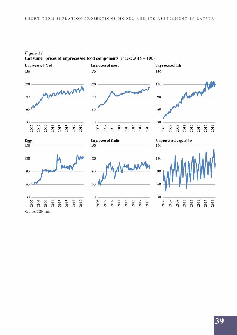
We model consumer prices of unprocessed food, disaggregating them into five components. We identify a long-run cointegration relationship between the respective consumer price component and its determinants, thus deriving a long-run level of each HICP component in a given period. There are two main factors affecting unprocessed food consumer prices in the long run – global food commodity prices4 and domestic labour costs (the latter reflect an upward trend in unprocessed food consumer prices; see Figure A1). Moreover, some consumer prices are also driven by car fuel prices and a negative long-run trend, which may reflect growing competition in the industry.

Table 1 Modelling unprocessed food prices: long-run elasticities and error correction coefficients

Error correction

Long-run coefficients Labour

costs Car fuel Global food Trend Constant

Unprocessed meat

–0.13*** (0.0187)

0.50*** (0.0618)

0.53*** (DG AGRI meat) (0.1055)

–0.002*** (0.0003)

Unprocessed fish

–0.12*** (0.0187)

0.33*** (0.0897)

0.36*** (0.1132)

0.50*** (Nasdaq salmon) (0.0870)

Eggs –0.11*** (0.0189)

0.47*** (0.0704)

0.23** (DG AGRI cereals) (0.1013)

Unprocessed fruits

–0.26*** (0.0419)

0.56*** (0.0684)

0.37*** (DG AGRI food) (0.0871)

–0.002*** (0.0004)

Unprocessed vegetables

–0.30*** (0.0551)

0.47*** (0.0620)

1.50*** (0.4074)

Source: authors' calculations. Notes. *, ** and *** defines statistical significance at 90%, 95% and 99% level respectively. Standard errors are in parentheses. Models are estimated using monthly data from January 2005 to December 2018. All variables are seasonally adjusted and expressed in logs. The lag order is selected by minimizing the Schwarz criterion. Time dummies are included in the estimation, but are not shown here and are available upon request.

Error correction seems to be particularly fast for unprocessed vegetables and unprocessed fruits, with 26%–30% of the adjustment towards fundamental price level taking place within one month (see Table 1). This implies that any idiosyncratic shock (i.e. not related to the changes in the respective drivers) tend to halve within 2–3 months (see Table A5). Such a fast price adjustment might reflect the fact that the respective consumer prices are highly volatile and depend on (rapidly changing) weather conditions.

Consumer prices of several unprocessed food items are closely linked to the global food commodity prices. The long-run elasticity of unprocessed meat consumer prices to the EU producer prices of meat is about 0.5. Elasticity of unprocessed fish consumer prices to international salmon price index is of similar magnitude. We do not find any statistically significant relationship between consumer prices of unprocessed fruits and the respective DG AGRI indices, which could reflect the fact that for many fruits DG AGRI prices are missing at least for some periods of time. Thus, we linked consumer prices of unprocessed fruits to the total DG AGRI food price index5. Furthermore, we linked consumer prices of eggs to DG AGRI prices of cereals, since

4 We tried to link consumer prices of unprocessed vegetables to EU producer prices of unprocessed vegetables, but forecast accuracy was worse than in the specification without it. 5 The DG AGRI food price index might reflect weather conditions in the region which are likely to affect also consumer prices of unprocessed fruits.


10

cereals are used as a feed for chickens and thus account for some part of egg production costs6.

The long-run elasticity of unprocessed food consumer prices to domestic labour costs is about 0.47–0.56, except for unprocessed fish which recorded somewhat lower elasticity at 0.33. Note that unprocessed fish prices are the only unprocessed food item showing a robust association with car fuel prices. Given that an increase in domestic labour costs leads to higher fuel price retail margins, the actual impact of labour costs on consumer prices of unprocessed fish tends to be somewhat higher than the long-run elasticity reported in Table 1 (this issue will be further addressed in Section 5).

Moreover, after taking into account observable fundamentals, we identify a negative trend in consumer prices of unprocessed meat and unprocessed fruits. This negative trend might reflect a growing competition among retailers or a greater availability of cheaper imports.

4.2 Processed food prices

We model consumer prices of processed food, disaggregating them into 12 components7. The monthly speed of adjustment towards the fundamental price level is somewhat slower than in the case of unprocessed food (often below 10%), with a notable exception of processed meat prices (18%). In all cases, however, error correction coefficients remain highly statistically significant (see Table 2).

In addition to global food commodity prices and domestic labour costs (with the latter reflecting the upward trend in processed food consumer prices; see Figure A2), some processed food prices are linked to the respective unprocessed food prices and nominal exchange rate developments.

The highest long-run elasticity of consumer prices to global food commodity prices is evident for the consumer prices of dairy products (as well as oils and fats)8 to the EU producer prices of dairy products at about 0.6–0.7. A high elasticity might reflect the fact that dairy is the only DG AGRI index, which partly consists of processed products ready for the final consumption (such as cheese9).

Elasticity of non-alcoholic beverages consumer prices to global coffee prices is somewhat lower at about 0.4. Also in this case, the magnitude of elasticity is feasible, taking into account that coffee accounts for about 45% of non-alcoholic beverage consumption. In turn, consumer prices of sugar and chocolate, as well as consumer prices of the miscellaneous component "other food" tend to follow international sugar prices, with elasticity somewhat lower than 0.3. Besides, "other food" consumer prices are linked to the total DG AGRI food index, reflecting the fact that many different food commodities can be used as ingredients for food products entering this miscellaneous HICP component.

6 We regard the egg consumer price elasticity to the DG AGRI cereals price index of about 0.2 as reasonable. 7 We do not find any explanatory variables for tobacco consumer prices (except strong correlations with changes in tobacco excise tax rates over time). Therefore, tobacco is projected judgementally (details are available upon request). 8 Butter accounts for about 40% of the latter HICP component. 9 This might be compared with the DG AGRI cereals price index containing, for instance, wheat and rye – commodities that should be processed extensively before the final usage.


11

Table 2 Modelling processed food prices: long-run elasticities and error correction coefficients

Error correction

Long-run coefficients Labour

costs Unprocessed

HICP Car fuel Global food Exchange

rate (NEER)

Trend Constant

Processed meat

–0.18*** (0.0190)

0.85*** (meat) (0.0156)

0.21*** (0.0680)

0.71*** (0.0718)

Processed fish

–0.07*** (0.0090)

0.21*** (0.0658)

0.18** (fish) (0.0740)

0.20*** (0.0551)

1.43*** (0.2997)

Processed fruits

–0.09*** (0.0158)

0.65*** (0.0490)

0.31*** (0.0903)

Processed vegetables

–0.08*** (0.0168)

0.81*** (vegetables)

(0.0769)

0.99*** (0.3361)

Dairy products

–0.11*** (0.0132)

0.41*** (0.0326)

0.20*** (0.0722)

0.57*** (dairy) (0.1125)

–1.67*** (0.2987)

Bread and cereals

–0.09*** (0.0098)

0.74*** (0.0707)

0.26*** (cereals) (0.0325)

–0.002*** (0.0004)

Oils and fats

–0.05*** (0.0102)

0.45*** (0.1000)

0.72*** (dairy) (0.2334)

Sugar and chocolate

–0.06*** (0.0142)

0.38*** (0.0520)

0.18*** (0.0826)

0.27*** (sugar) (0.0633)

Other food –0.07*** (0.0099)

0.33*** (0.0450)

0.31*** (food) (0.0649)

0.22*** (sugar) (0.0340)

Non-alcoholic beverages

–0.11*** (0.0115)

0.16*** (0.0368)

0.27*** (0.0558)

0.42*** (coffee) (0.0421)

Alcoholic beverages

–0.08*** (0.0145)

0.24*** (0.0482)

0.10*** (cereals) (0.0390)

2.56*** (0.2475)

Source: authors' calculations. Notes. *, ** and *** defines statistical significance at 90%, 95% and 99% level respectively. Standard errors are in parentheses. Models are estimated using monthly data from January 2005 to December 2018. All variables are seasonally adjusted and expressed in logs. Time dummies are included in the estimation, but are not shown here and are available upon request. The lag order was selected by minimizing the Schwarz criterion.

The DG AGRI cereals price index tends to affect two consumer price components – bread and cereals, as well as alcoholic beverages. A moderate elasticity in bread and cereals points to the fact that the price of grain accounts for a minor part of bread production costs.10 Elasticity is even lower for alcoholic beverages: despite the fact that cereals are used in the production of some alcoholic beverages like spirits and beer, other factors like labour costs and excise taxes tend to be even more important for the formation of consumer prices of alcoholic beverages11.

Several HICP components of processed food are linked to the respective unprocessed food components. This causal link is particularly evident for the prices of meat, fish, and vegetables. Note that this specification implies that the factors affecting

10 Cereals account for approximately 10% of bread production costs (newspaper Dienas Bizness, issue 17 (5336), 24 January 2017). 11 The impact of excise tax change on the consumer prices of alcoholic beverages is added as an expert judgement (separately for several types of alcoholic beverages, such as spirits, wine and beer).


12

unprocessed food prices have an indirect impact on processed food components12. We also document a statistically significant link between consumer prices of several processed food components and the retail prices of car fuel (with long-run elasticity of about 0.2–0.3).

Furthermore, consumer prices of all processed food components are explicitly or implicitly linked to domestic labour costs. In other words, labour costs either directly enter the equation of the respective processed food item or its impact is indirect, with the effect coming from either unprocessed food item or car fuel prices. The magnitude of elasticities broadly reflect the share of labour costs and transportation costs in the respective industry. For instance, in the case of dairy products (as well as of sugar and chocolate), the elasticity of consumer prices to labour costs is at least twice higher than to car fuel. On the contrary, consumer prices of non-alcoholic beverages tend to react to car fuel prices more than to domestic labour costs. Overall, the elasticity of processed food consumer prices to domestic labour costs is broadly similar to that of global food commodity prices, suggesting that these two cost components are similarly important.

In addition, we document a positive relation between consumer prices of processed meat and the NEER. It might reflect large meat imports from Poland13 – a country whose currency showed large exchange rate fluctuations vis-à-vis the euro during the past 15 years. Besides, after taking into account observable fundamentals of consumer prices of bread and cereals, we get a negative trend in the residuals. Thus, we explicitly add a trend into the respective long-run equation, reflecting the growing competition in the industry14.

4.3 Energy prices

We distinguish five components of HICP energy prices: car fuel, natural gas, heat energy, electricity and solid fuel. Consumer prices of the first three components correlate with prices of oil products. The link between crude oil prices and consumer car fuel prices is quite straightforward, but the link with other two energy prices is fragmented, i.e. consumer prices of natural gas tend to change infrequently, and both natural gas and heat energy are subject to administrative regulations. We do not observe any statistically significant link between electricity and global oil prices. In turn, solid fuel prices react to developments in producer prices of timber.

Developments in car fuel consumer prices strongly reflect movements in crude oil prices in global markets. We model these relationships in the spirit of Meyler (2009) – from upstream to downstream prices – accounting for refining, distribution, retailing margins and indirect taxes. The equations below (see Table 3) depict elasticities where

12 For instance, despite the fact that labour costs are not explicitly included in the processed meat equation, the domestic labour cost shock transmits to prices of processed meat via the unprocessed meat component (see Section 5). A similar story applies to the consumer prices of processed vegetables as well. 13 Poland is a main exporter of meat products to Latvia, accounting for more than a quarter of total meat imports over 2005–2018. 14 For instance, Kārlis Zemešs, Chief of the Latvian Bakers Association, said that the bread baking industry in Latvia faces an ever-increasing competition from many small producers entering the market and from some supermarkets building their own bread baking facilities (LSM.LV, 2014). Available: https://www.lsm.lv/raksts/zinas/ekonomika/maizes-tirgu-siva-konkurence-un-aizvien-vairak-majrazotaju.a81640/. There is also an anecdotal evidence that the bread variety has increased markedly (produced by many different firms) over the past 15 years in a typical Latvian supermarket, and this is likely to hinder an increase in consumer prices.

https://www.lsm.lv/raksts/zinas/ekonomika/maizes-tirgu-siva-konkurence-un-aizvien-vairak-majrazotaju.a81640/

https://www.lsm.lv/raksts/zinas/ekonomika/maizes-tirgu-siva-konkurence-un-aizvien-vairak-majrazotaju.a81640/


13

crude oil prices pass to refined petrol and diesel prices (both in EUR per litre)15. Elasticities are close to one in both cases, meaning that an oil price increase by 1 euro cent per litre translates into the price increase of refined petrol and refined diesel by about 1 euro cent. At the next stage, refined oil prices feed into retail consumer prices without taxes (both in euro per litre). Again, elasticities are close to one for retail prices of both petrol and diesel. Finally, we add excise and VAT taxes, which account for a large share in car fuel consumer prices (see Figure A3)16.

Table 3 Modelling car fuel prices: long-run elasticities and error correction coefficients

Error correction

Oil (euro) Refined prices

Labour costs Trend Constant

Refined petrol –0.09*** (0.0141)

0.95*** (0.0416)

0.00006*** (0.00002)

Refined diesel –0.06*** (0.0110)

1.12*** (0.0377)

Retail petrol –0.10*** (0.0155)

0.99*** (0.0344)

0.00006*** (0.00002)

0.08*** (0.018)

Retail diesel –0.17*** (0.0203)

1.04*** (0.0172)

0.00008*** (0.00001)

0.07*** (0.0103)

Source: authors' calculations. Notes. *, ** and *** defines statistical significance at 90%, 95% and 99% level respectively. Standard errors are in parentheses. Models are estimated using weekly data from January 2005 to December 2018. All variables are expressed in euro per litre. The lag order is selected by minimizing the Schwarz criterion. Time dummies are included in the estimation, but are not shown here and are available upon request.

There is also a strong long-term link between crude oil prices and the consumer prices of natural gas and heat energy. The price formation policy of the main natural gas supplier AS Latvijas Gāze states that the prices of natural gas depend on the average quotations of gas oil and diesel prices over the last nine months and the developments of the USD/EUR exchange rate17. Prices of natural gas for households are adjusted twice a year (in January and July), thus the speed of a pass-through is fairly slow.

Several major Latvian cities produce heat energy mainly from natural gas, and this fact implies a link between oil and heat energy prices. The medium-term elasticity of natural gas and heat energy consumer prices to the crude oil price is about 0.5–0.6 (see Figure 2). Since natural gas and heating tariffs are subject to administrative regulation (changes in tariffs must be approved by the PUC before they can take effect), the speed of the pass-through may vary from time to time. Therefore, we do not explicitly model natural gas and heat energy prices as a function of oil price but rather forecast them judgementally against the background of recent oil price dynamics and publicly available information on tariff approvals (or rejections) by the PUC and new tariff proposals sent by service providers to the PUC.

15 Note that petrol and diesel prices are the only HICP items whose prices are modelled in euro per litre rather than in logs. See Meyler (2009) on the merits of levels versus logs in the forecasting of car fuel prices. 16 The consumer price index of car fuel (which then is employed in modelling consumer prices of some food products and services) is obtained as the weighted average of retail consumer prices of diesel and petrol. 17 https://lg.lv/majai/tarifi-un-kalkulators.

https://lg.lv/majai/tarifi-un-kalkulators


14

Figure 2 Consumer prices of natural gas and heat energy in Latvia (index: 2015 = 100) and crude oil prices

Sources: CSB and Bloomberg data and authors' calculations. Notes. The numbers near the dots represent years over the period 2005–2018.

The connection to the Nord Pool electricity market implies that electricity wholesale prices in Latvia strongly correlate with the respective prices in Estonia, Lithuania and the Scandinavian countries. Since a large share of electricity in the region is produced by hydropower plants, we do not observe any statistically significant link between global oil prices and electricity wholesale prices. In fact, electricity consumer prices follow electricity wholesale prices with a lag. Although the electricity market in Latvia was liberalised in 2015, AS Latvenergo is still the major supplier of electricity to households. In addition, as the majority of households have fixed-price contracts with the electricity supplier (implying that the electricity price changes, e.g. once a year, taking into account the electricity wholesale price during the previous period), the consumer price of electricity changes infrequently18, and behaviour of electricity prices resembles that of administered prices. Consumer solid fuel prices in Latvia mainly represent the price of firewood. Thus, we link solid fuel prices to Latvian timber prices and domestic labour costs (see Table 4).

Table 4 Modelling firewood prices: long-run elasticities and error correction coefficients

Error correction Timber Labour costs Solid fuel –0.07***

(0.0117) 0.50*** (0.1505)

0.41*** (0.0843)

Source: authors' calculations. Notes. *, ** and *** defines statistical significance at 90%, 95% and 99% level respectively. Standard errors are in parentheses. Models are estimated using monthly data from January 2005 to December 2018. All variables are seasonally adjusted and expressed in logs. The lag order is selected by minimizing the Schwarz criterion. Time dummies are included in the estimation, but are not shown here and are available upon request.

18 For instance, the consumer price of electricity rose by almost 11% in January 2019 when AS Latvenergo adjusted the fixed-term electricity tariff to reflect an increase in electricity wholesale prices in the second half of 2018 (electricity supply generated by hydropower plants located in the Baltics and Scandinavian countries decreased due to the hot and dry summer).


15

4.4 Non-energy industrial goods prices

Developments in prices of individual NEIG items exhibited different patterns over the last 15 years (see Figure A4). The prices of durable goods (motor cars, refrigerators, etc.) were broadly stable up to 2008 and then significantly and monotonically decreased over the last 10 years (see Figure A5). The major share of these goods is imported (see Figure A6)19, and their prices depend mainly on the euro exchange rate and hardly measurable factors, such as global technical progress or an increasing integration of developing countries with low labour costs into global value chains.

Consumer prices of semi-durable goods (mainly clothes and footwear) show considerable seasonality, and many years have seen the price level remain almost unchanged. Semi-durable goods prices increased moderately up to 2008, most likely reflecting the growing domestic demand. But in the aftermath of the financial crisis, the prices somewhat decreased and have remained relatively stable since then. Although the manufacturing of clothes in Latvia is gradually becoming costlier due to rising labour costs, the availability of cheap imports counterbalances the impact of the production cost increases on consumer prices of clothes.

In turn, consumer prices of non-durable industrial goods (soap, newspapers, medicines, etc.) tend to rise over time. The share of imported goods here is considerably lower, and this is the only group of industrial goods whose prices significantly correlate with domestic economic activity both in Latvia and the EU (see Figure A7).

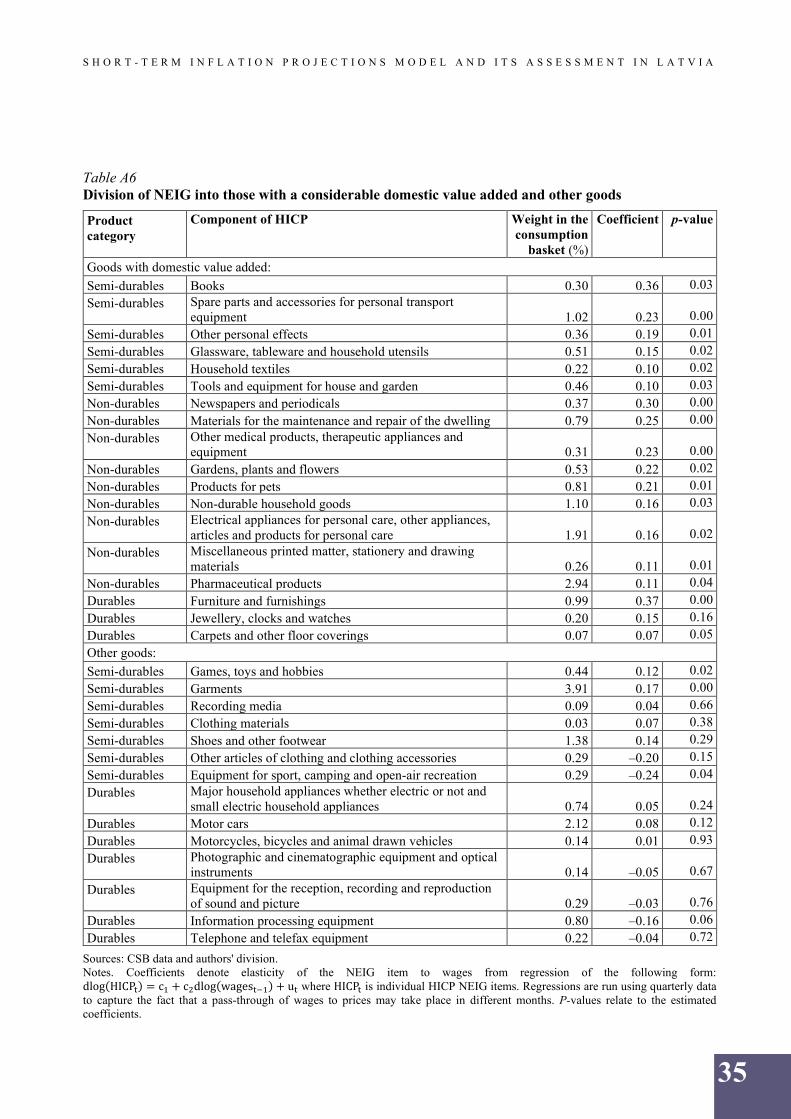
In order to understand which NEIG prices are driven by domestic economic activity and share correlations with domestic labour costs, we regress each NEIG item on labour costs separately. Then we aggregate those NEIG items, which show statistically significant correlations with labour costs, and build a special aggregate, which we call industrial goods with domestic value added20 further in the text. These goods account for more than a half in consumer spending on industrial goods (see Table A6)21. The long-run elasticity of industrial goods with domestic value added to domestic labour costs is about 0.30 (see Table 5). As some of these goods are imported, we find a positive correlation of consumer prices with the NEER. We also include a negative trend in cointegration relationship of NEIG consumer prices, which are likely to reflect the increasing competition or greater availability of cheap imports22.

19 A precise import share is not known, since products imported to Latvia could then be re-exported to other countries. 20 This definition does not necessarily mean that these products are made in Latvia. The definition rather reflects the correlation with domestic labour costs, which might represent domestic value added of the good. 21 Other NEIG items, which are not included in the aggregate of industrial goods with domestic value added, are either largely imported or represent administered public utilities like water supply (see "Other goods" in Table A6). Other NEIG items are forecasted with expert judgements. 22 There is an anecdotal evidence that the number of large department stores and supermarkets increased markedly in Latvia during the last 15 years. Also, imports from China increased almost five times between 2005 and 2018.


16

Table 5 Modelling NEIG prices: long-run elasticities and error correction coefficients

Error correction

Long-run coefficients Labour costs NEER Trend

NEIG with domestic value added –0.11*** (0.0123)

0.30*** (0.0204)

0.26* (0.1390)

–0.001*** (0.0002)

Source: authors' calculations. Notes. *, ** and *** defines statistical significance at 90%, 95% and 99% level respectively. Standard errors are in parentheses. Models are estimated using monthly data from January 2005 to December 2018. All variables are seasonally adjusted and expressed in logs. The NEER is defined as an increase means depreciation. The lag order is selected by minimizing the Schwarz criterion. Time dummies are included in the estimation, but are not shown here and are available upon request.

4.5 Services prices

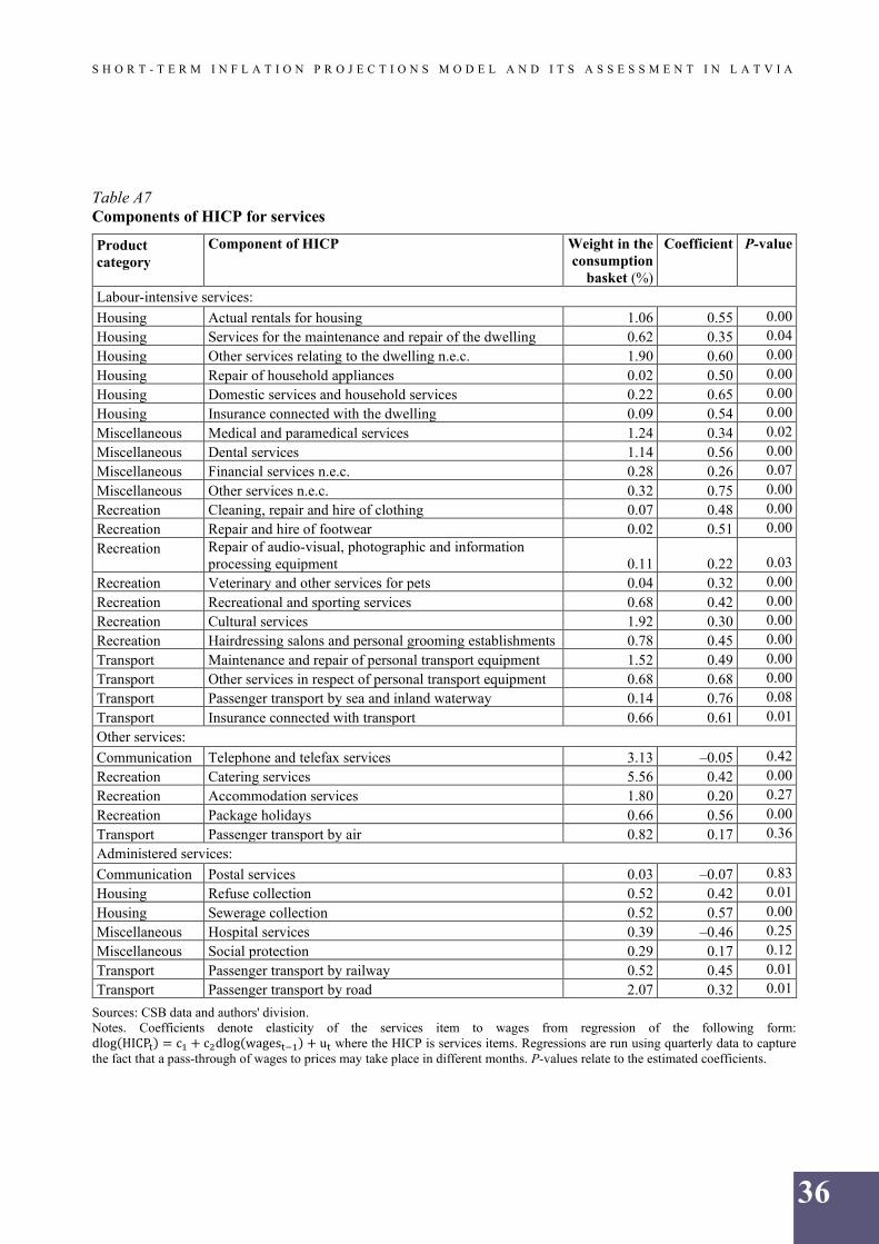
Components of services prices reflect different behaviour patterns and trends. Therefore, we divide all services prices in eight groups: catering, communication, accommodation, air transport, package holidays, education, administrative and other market services (hereinafter, labour-intensive services) and model them separately (see Figure A8).

Labour-intensive services are the largest group of services (see Table A7; more than 40% of total services) sharing a common price dynamics and exhibiting a very high long-run price elasticity to labour costs (0.77; see Table 6). Likewise, a high elasticity to labour costs is also observed in catering services (the share in total services constitutes almost 20%) whose prices in cafes and restaurants also depend on developments in consumer prices of food products.

Table 6 Modelling services prices: long-run elasticities and error correction coefficients

Error correction

Long-run coefficients Labour costs HICP item Other variables Trend Constant

Labour-intensive services

–0.14*** (0.0176)

0.77*** (0.0276)

–0.001*** (0.0001)

Catering –0.11*** (0.0173)

0.75*** (0.0479)

0.12** (food) (0.0530)

–0.001*** (0.0002)

Communication –0.02*** (0.0025)

0.89*** (0.3114)

–0.96*** (internet usage, %)

(0.3347)

2.80** (1.4109)

Accommodation –0.28*** (0.0370)

0.10** (0.0494)

0.38*** (hotel occupancy;

%) (0.0402)

–0.002*** (0.0002)

Air transport –0.06*** (0.0143)

0.76*** (fuel) (0.2538)

–0.005*** (0.0017)

Package holidays –0.19*** (0.0385)

0.50*** (0.0693)

0.32** (air transport)

(0.1258)

–0.001** (0.0005)

Source: authors' calculations. Notes. *, ** and *** defines statistical significance at 90%, 95% and 99% level respectively. Standard errors are in parentheses. Models are estimated using monthly data from January 2005 to December 2018. All variables are seasonally adjusted and expressed in logs. The lag order is selected by minimizing the Schwarz criterion. Time dummies are included in the estimation, but are not shown here and are available upon request. HICP for food means HICP for food prices, excluding alcohol and tobacco.

Accommodation prices and those of package holidays are highly volatile owing to seasonal fluctuations and calendar effects like Easter holidays (see Figure A8). For


17

these reasons, we model them separately. Incorrect accounting of these features may inflict large forecast errors over the short-term horizon. Consumer prices of both accommodation services and package holidays respond to domestic labour costs, but to a smaller extent than consumer prices of labour-intensive or catering services. Accommodation prices are largely determined by demand and supply interactions reflected in the hotel room occupancy rate. In turn, package holidays prices are affected both by labour costs and prices of air transport, since package holidays are defined as holidays whose costs of travel and accommodation are bundled and sold in one transaction.

Furthermore, we link consumer prices of air transport to the costs of fuel and labour23, while the prices of communication services – to labour costs and internet usage24.

Administered prices are singled out and modelled separately. They are postal services, refuse and sewerage collection, hospital services, social protection and passenger transport by railway and road (see Figure A10). These items are characterised by one-off tariff increases, which eventually are driven by rising domestic labour costs. Although, compared to labour-intensive services, administered price changes are infrequent and may exhibit a long period of standstill. Hence, it is not reasonable to model administered prices econometrically in the short to medium term. Instead, we project prices of administered services judgementally using publicly available information (any changes in tariffs must be approved by the PUC and therefore they have to be submitted to the PUC in advance).

Education services prices are not regarded as administered, but the dynamics of education prices resemble administered behaviour. Education price changes mainly occur in September (see Figure A11), reflecting the beginning of an academic year25. The systematic pattern of education price changes motivates us to forecast this item also judgementally.

5. THE IMPACT OF DOMESTIC AND FOREIGN SHOCKS

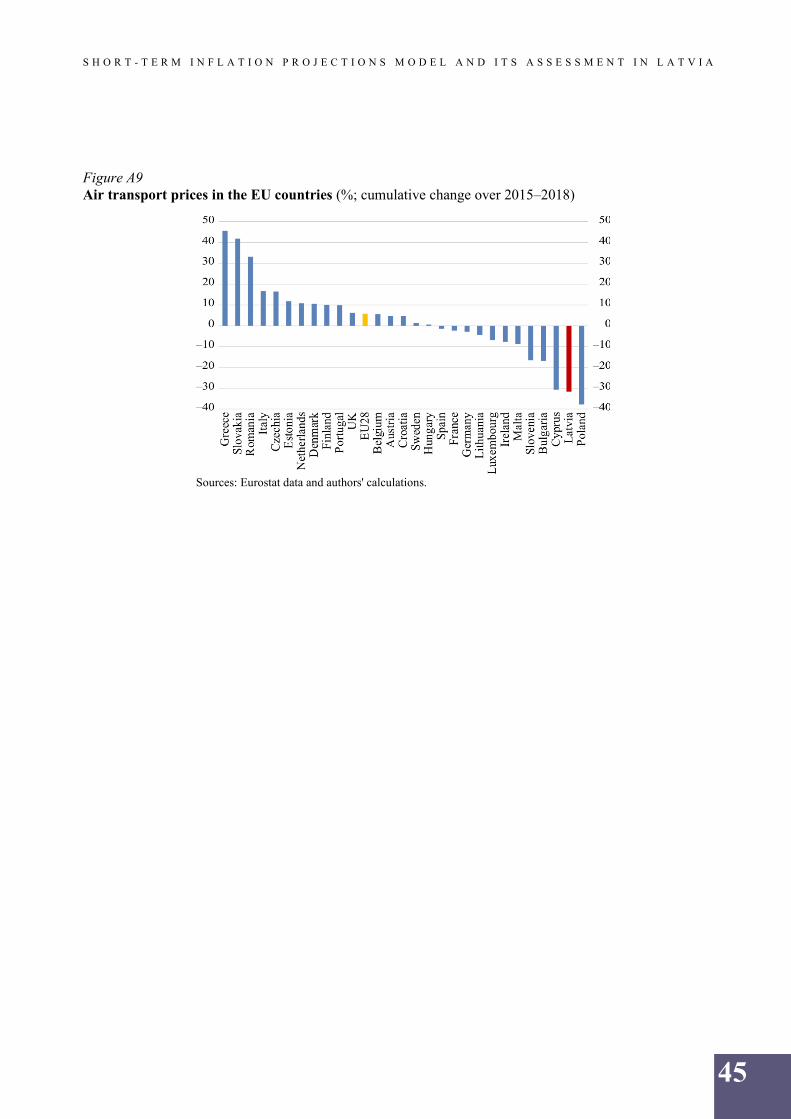
This section examines the pass-through of three main domestic and foreign shocks to consumer prices in Latvia, taking into account both direct and indirect effects. We estimate models over the period 2005–2018 (using monthly data) and simulate a permanent 10% upward shock to the main determinants of Latvian consumer prices starting in January 2019. Hence, the pass-through in this section is defined as a percentage deviation from the baseline. We differentiate between the impact of global

23 According to the International Air Transport Association, 25% of total operating expenses in the global airline industry are determined by fuel costs and 23% – by labour costs (https://www.iata.org/publications/economics/Reports/Industry-Econ-Performance/Airline-Industry-Economic-Performance-Jun19-Report.pdf). However, in Latvia air transport prices react to domestic labour costs substantially weaker than to fuel prices. This might reflect the fact that labour costs in aviation are largely determined internationally and therefore might not mirror directly the developments of domestic labour costs. The competition is also quite fierce in the Latvian market – from 2014 through 2018, air transport prices in Latvia dropped by 32% which is one of the largest declines among EU countries (see Figure A9). 24 Prices of communication services are substantially affected by the adoption of technical innovations and broadening the number of clients. Prices of communication services decreased considerably over the last 15 years, and during this period the number of internet users significantly increased. The cause and effect relationship is most probably bilateral in this case – the large number of internet users reduced maintenance costs of the internet infrastructure per client, fostering availability of the internet at a lower price. Internet access at a lower price successfully attracted even a larger number of internet users. 25 Most of education institutions in Latvia are public and financed through government funding.

https://www.iata.org/publications/economics/Reports/Industry-Econ-Performance/Airline-Industry-Economic-Performance-Jun19-Report.pdf

https://www.iata.org/publications/economics/Reports/Industry-Econ-Performance/Airline-Industry-Economic-Performance-Jun19-Report.pdf


18

food commodity prices, crude oil prices and domestic labour costs (proxied by average wage rate).

5.1 Pass-through of global food commodity prices to consumer prices

Global food commodity prices affect food consumer prices in Latvia both directly and indirectly. Direct effects stem from the impact of global food prices on prices of unprocessed and processed food. Indirect effects stem from the impact of selected unprocessed food prices on prices of processed food and the impact of total food prices (excluding alcohol and tobacco) on catering services.

A permanent 10% increase in global prices of food commodities raises Latvian consumer prices by 0.9% in the medium term. This estimate is slightly higher than in other EU countries (Ferrucci et al. (2012) and Peersman (2018)) since food products in Latvia have a larger share in the consumption basket. Our estimates show that two thirds of the pass-through from global food commodity prices to consumer prices in Latvia take place during the first year.

There exists a close relation between global food commodity prices and food consumer prices in Latvia26 (see Tables 1 and 2). When global food commodity prices change considerably, Latvian consumer prices follow with a lag of a few months. There were several episodes over the last eight years of this price co-movement. For instance, food consumer prices in Latvia were significantly affected by a simultaneous increase in various global food commodity prices in 2011: dairy consumer prices were affected by an increase in global dairy prices in 2017; and sugar and coffee consumer prices were affected by a fall in global sugar and coffee prices at the turn of 2017 and 2018 (see Figure 3).

Figure 3 "Heat map" of global food prices and food consumer prices in Latvia (2011–2019)

Source: authors' calculations based on EC, Bloomberg and CSB data. Notes. The red colour denotes inflation above the long-term trend. The blue colour denotes inflation below the long-term trend. The brighter the colour, the greater the inflation deviation from the long-term trend. We normalize the annual inflation rate to take into account differences in long-term trends and volatility across series by subtracting the component-specific mean and dividing by its standard deviation.

When EU producer prices of dairy products increase by 10%, Latvian consumer prices of dairy products (milk, sour cream, curd, etc.), as well as consumer prices of oils and fats (a product category in which butter has a big share), rise by about 6%. The speed of the pass-through is faster for dairy products compared to oils and fats, reflecting

26 As a global price of food commodities, we employ either EU producer prices (cereals, dairy, meat, total food), Nasdaq prices (salmon) or global wholesale prices (sugar and coffee).


19

the fact that the expiry date for the largest part of dairy products is considerably shorter than for butter (see Figures 4 and A12).

Figure 4 Pass-through of a 10% increase in the global food commodity prices to consumer prices of food products in Latvia (%)

Source: authors' calculation based on EC and CSB data. Note. Estimates are made over the 2005–2018 period using monthly data; the simulation assumes a 10% increase in global prices of food commodities starting in January 2019.

Our estimates show that a 10% increase in EU meat producer prices raises Latvian consumer prices for unprocessed meat (pig meat, beef, chicken, etc.) by 5.1% and consumer prices of processed meat products (sausages, ravioli, etc.) by 4.5%. In the latter case, the pass-through takes a considerably longer time (half of the impact can be seen after five and nine months respectively).

EU producer prices of cereals affect Latvian consumer prices of bread and cereals, eggs, as well as alcoholic beverages. The impact on alcoholic beverage prices is considerably lower and the pass-through is also slower, reflecting a small share of cereals in production costs, as well as a relatively long storage term.


20

Pass-through is relatively slow also in the case of global prices of sugar affecting Latvian consumer prices of sugar and chocolate, and global coffee prices affecting consumer prices of non-alcoholic beverages: half of the impact could be recorded after eight and nine months respectively.

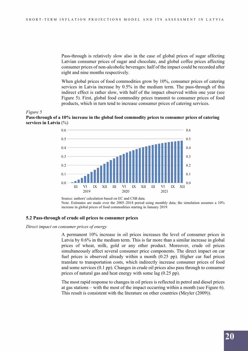
When global prices of food commodities grow by 10%, consumer prices of catering services in Latvia increase by 0.5% in the medium term. The pass-through of this indirect effect is rather slow, with half of the impact observed within one year (see Figure 5). First, global food commodity prices transmit to consumer prices of food products, which in turn tend to increase consumer prices of catering services.

Figure 5 Pass-through of a 10% increase in the global food commodity prices to consumer prices of catering services in Latvia (%)

Source: authors' calculation based on EC and CSB data. Note. Estimates are made over the 2005–2018 period using monthly data; the simulation assumes a 10% increase in global prices of food commodities starting in January 2019.

5.2 Pass-through of crude oil prices to consumer prices

Direct impact on consumer prices of energy

A permanent 10% increase in oil prices increases the level of consumer prices in Latvia by 0.6% in the medium term. This is far more than a similar increase in global prices of wheat, milk, gold or any other product. Moreover, crude oil prices simultaneously affect several consumer price components. The direct impact on car fuel prices is observed already within a month (0.25 pp). Higher car fuel prices translate to transportation costs, which indirectly increase consumer prices of food and some services (0.1 pp). Changes in crude oil prices also pass through to consumer prices of natural gas and heat energy with some lag (0.25 pp).

The most rapid response to changes in oil prices is reflected in petrol and diesel prices at gas stations – with the most of the impact occurring within a month (see Figure 6). This result is consistent with the literature on other countries (Meyler (2009)).


21

Figure 6 Transmission of a 10 euro cents increase in oil prices to diesel and petrol prices before taxes

Source: authors' calculation based on EC and CSB data. Notes. The horizonal axis denotes the number of weeks, the vertical one – euro cents. Estimates are made over the 2005–2018 period using weekly data; the simulation assumes a 10 euro cents increase in crude oil price per litre in the first week of 2019.

Note that the car fuel price elasticity to the oil price is positively related to the oil price. This is due to the fact that a large share of final consumer fuel prices comprises taxes (the excise tax and VAT). The higher the price of oil, the greater the share of oil in the price of fuel (while the share of taxes is smaller), the greater the elasticity (see Figure 7).

Figure 7 Pass-through of a 10% increase in oil price to car fuel consumer prices depending on the initial oil price

Source: authors' calculations. Note. Calculations are based on the 2018 average fuel margins and tax rates.

One might point out that car fuel prices might be more responsive to oil price increases than decreases (e.g. Latvian retail car fuel prices in 2019 increased by half compared to 2005–2006, although the level of oil prices in 2019 was approximately the same as in 2005–2006, around 50–60 US dollars per barrel). There are three reasons behind these observations. First, the euro depreciated against the US dollar by one-seventh over the last 15 years (this means a higher crude oil price in the euro currency, all else equal). Second, excise tax rates on car fuel have almost doubled since 2005. Third, rising labour costs affect car fuel retail margins. We take into account all these factors when projecting inflation. While the car fuel price elasticity to domestic labour costs


22

is not high – indeed, it is much lower than its elasticity to oil prices – even this factor alone can contribute to a rise in fuel prices without any oil price changes (see Figure 8).

Figure 8 Car fuel price structure (euro per litre)

Source: authors' calculations. Notes. The distribution and retail margin reflects costs related to the delivery of car fuel to gas stations, the costs of gas station maintenance, as well as the profits. The car fuel price is defined as an average of petrol and diesel prices.

Although consumer prices of natural gas and heat energy tend to follow global prices of crude oil in the medium and long-term horizon, these consumer prices are administered by authorities (see Section 4). This precludes us from explicitly modelling them as a function of crude oil price developments.

Indirect effects on consumer prices of food products and services

Most food prices respond statistically significantly to the changes in car fuel prices and thus to the changes in crude oil prices. For example, a 10% increase in crude oil prices raises the prices of fish, non-alcoholic beverages and processed fruits by about 1.0%–1.2% and those of dairy products and confectionary – by 0.6% (see Figure 9).

Figure 9 Pass-through of a 10% increase in oil price to consumer prices of selected food products in Latvia (%)

Source: authors' calculations. Note. Estimates are made over the 2005–2018 period using monthly data; the simulation assumes a permanent increase in the oil price by 10% as from January 2019.


23

We identify two services components, which significantly react to the changes in crude oil prices, i.e. consumer prices of air transport and package holidays. Crude oil prices affect air transport prices to a much greater extent than domestic labour costs which possibly reflects the fact that airline companies tend to recruit their staff internationally (see Section 4). The prices of package holidays represent the costs of travel (mainly air fare prices) and accommodation (see Figure 10).

Figure 10 Pass-through of a 10% increase in oil price to consumer prices of selected services in Latvia (%)

Source: authors' calculations. Note. Estimates are made over the 2005–2018 period using monthly data; the simulation assumes a permanent increase in oil price by 10% as from January 2019.

5.3 Pass-through of wages to consumer prices

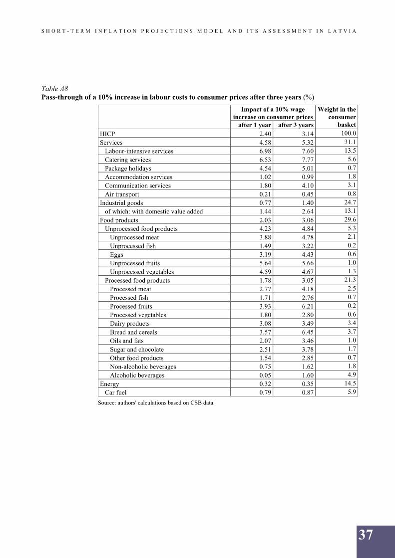
Labour costs are an important part of production costs in every firm. Thus, an increase in wages transmits to increases in consumer prices after some time. However, the impact of labour costs on prices differs both in time and magnitude for all goods produced and services provided (see Table A8).

Services and NEIG

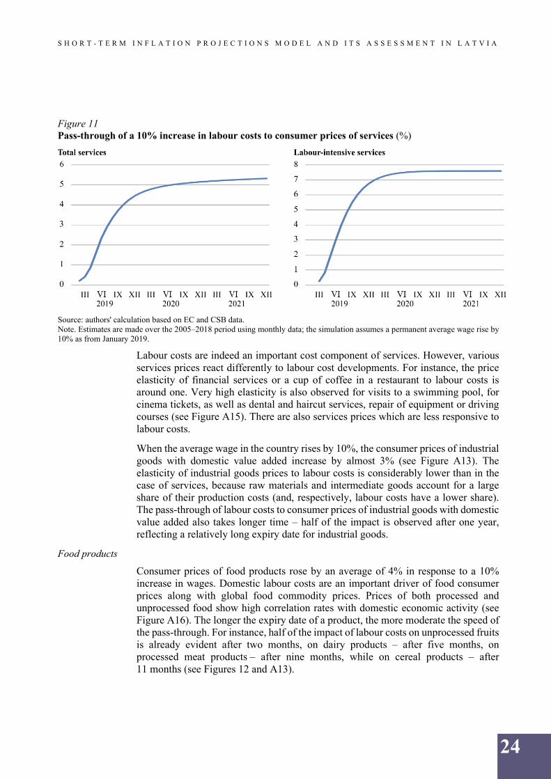
An increase in labour costs has the largest impact on the prices of services, since the provision of services is typically more labour intensive than the production of goods. When the average wage in the country grows by 10%, services prices increase by more than 5% in the medium term (over three years), and half of this impact is seen after six months. The pass-through of domestic labour costs is particularly robust to consumer prices of labour-intensive and catering services (see Figures 11 and A13). A strong empirical relation between economic activity and consumer price inflation is evident also in the EU. The countries with the fastest economic growth likewise experienced the steepest rise in services prices over the last 20 years (see Figure A14).


24

Figure 11 Pass-through of a 10% increase in labour costs to consumer prices of services (%)

Source: authors' calculation based on EC and CSB data. Note. Estimates are made over the 2005–2018 period using monthly data; the simulation assumes a permanent average wage rise by 10% as from January 2019.

Labour costs are indeed an important cost component of services. However, various services prices react differently to labour cost developments. For instance, the price elasticity of financial services or a cup of coffee in a restaurant to labour costs is around one. Very high elasticity is also observed for visits to a swimming pool, for cinema tickets, as well as dental and haircut services, repair of equipment or driving courses (see Figure A15). There are also services prices which are less responsive to labour costs.

When the average wage in the country rises by 10%, the consumer prices of industrial goods with domestic value added increase by almost 3% (see Figure A13). The elasticity of industrial goods prices to labour costs is considerably lower than in the case of services, because raw materials and intermediate goods account for a large share of their production costs (and, respectively, labour costs have a lower share). The pass-through of labour costs to consumer prices of industrial goods with domestic value added also takes longer time – half of the impact is observed after one year, reflecting a relatively long expiry date for industrial goods.

Food products

Consumer prices of food products rose by an average of 4% in response to a 10% increase in wages. Domestic labour costs are an important driver of food consumer prices along with global food commodity prices. Prices of both processed and unprocessed food show high correlation rates with domestic economic activity (see Figure A16). The longer the expiry date of a product, the more moderate the speed of the pass-through. For instance, half of the impact of labour costs on unprocessed fruits is already evident after two months, on dairy products – after five months, on processed meat products – after nine months, while on cereal products – after 11 months (see Figures 12 and A13).


25

Figure 12 Pass-through of a 10% increase in labour costs to selected consumer food prices in Latvia (%)

Source: authors' calculation using EC and CSB data. Note. Estimates are made over the 2005–2018 period using monthly data; the simulation assumes a permanent average wage rise by 10% as from January 2019.

The impact of labour costs on consumer food prices in Latvia is also clearly seen at a more detailed product level. The gap between the consumer price of a particular food product in Latvia and the global food commodity price widens exactly on the occasions when wages face strong growth. For instance, the dynamics of labour costs in Latvia describe well why the retail price of sour cream in the long run rises faster than producer prices of milk. Increasing labour costs also give an answer why the prices of white bread in a supermarket correlate more with the rises rather than decreases of wheat producer prices (see Figure A17).

6. FORECAST EVALUATION

This section follows a formal model evaluation exercise. First, we assess model adequacy in terms of RMSFEs and compare the results with a benchmark model. Second, we compare forecasts of the STIP model with the forecasts submitted by Latvijas Banka to the ECB under NIPE forecast rounds. The latter comparison gives us an intuition on the degree of improvement over current forecasting practices employed by Latvijas Banka.

We conduct an out-of-sample forecast evaluation exercise in order to simulate forecast errors as if they were generated in real time. We run the out-of-sample forecasting exercise from January 2014 to December 2018. The reason behind the choice of the starting date is the following. Latvia joined the euro area in January 2014, and Latvijas Banka regularly contributes inflation projections to the BMPE. This provides us with a unified set of assumptions, enabling us to assess the performance of the STIP model against these assumptions. Second, this allows us to compare directly the performance of the STIP model with current forecasting practices which is essential in promotion of new methods. Third, the size of the out-of-sample is roughly one third of the whole sample, and two thirds of the sample is used for the in-sample estimation, so the proportion could be regarded as adequate.


26

We closely follow Giannone et al. (2014) notation in setting up an evaluation exercise. First, let us define 𝑝𝑝𝑡𝑡 as the natural logarithm of the consumer price index under consideration. Then the target variable is h-period ahead the change in prices as follows:

𝜋𝜋𝑡𝑡+ℎ = 𝑝𝑝𝑡𝑡+ℎ − 𝑝𝑝𝑡𝑡 (3).

For each month we make projections 12 months ahead (horizon h) using the STIP model and store forecasts. Further, we compare forecasts with outturns and obtain the RMSFE as follows:

𝑅𝑅𝑅𝑅𝑅𝑅𝑅𝑅𝐸𝐸ℎ = � 1𝐾𝐾ℎ∑ �𝜋𝜋𝑣𝑣,𝑣𝑣+ℎ + 𝜋𝜋𝑣𝑣+ℎ�

2𝐷𝐷𝐷𝐷𝐷𝐷2018−ℎ𝑣𝑣=𝐽𝐽𝐽𝐽𝐽𝐽2014 (4).

𝐾𝐾ℎ is the number of forecast vintages between January 2014 and December 2018 for horizon h; 𝜋𝜋𝑣𝑣,𝑣𝑣+ℎ is the change in prices for the date v+h using vintage data v, and 𝜋𝜋𝑣𝑣+ℎ is the observed change in prices h periods ahead.

We select a random walk model with a drift as a benchmark model. The random walk model is a conventional model in the literature on inflation forecasting frequently used to compare with a competing model, and, as argued in the literature, the random walk model is hard to beat. A drift in the random walk is a natural extension as we work with level data. The random walk is defined as follows:

𝑝𝑝𝑡𝑡 = 𝛽𝛽0 + 𝛽𝛽1𝑝𝑝𝑡𝑡−1 + 𝑢𝑢𝑡𝑡 (5)

where 𝛽𝛽1 is set to one.

The STIP model contains various explanatory variables and requires pre-determined observations over the forecast horizon in order to obtain forecasts. Pre-determined observations are usually called assumptions. In line with the ESCB forecasting framework, euro area countries develop their inflation projections based on a particular set of common assumptions. More specifically, global prices, i.e. international food commodity prices (DG AGRI prices), crude oil prices and the exchange rate, are relevant assumptions for domestic prices. In turn, labour costs are projected internally. As a result, we compile a database of each assumption at every vintage of time used in the production of STIP forecasts to mimic forecasts in real time. Other explanatory variables like internet users or the hotel occupancy rate, which appear in the STIP model, we set to follow the random walk.

The STIP model also includes a number of consumer prices, which are not modelled due to various circumstances. However, they are integral in order to obtain special aggregates (e.g. processed food) and the headline consumer price index. Mainly these are administered prices (e.g. refuse and sewerage collection, etc.) or quasi-administered ones like natural gas prices and also those of tobacco, which is heavily taxed. These prices are also assumed to follow a random walk with a drift over the forecast horizon.

We summarize the results of the forecast evaluation exercise in Tables 7 and A9. First, the forecast errors of the STIP model are more accurate compared to the random walk. The ratio of STIP forecast errors to random walk less than one indicates an improvement of STIP forecasts over the random walk. Across components, the forecast accuracy gains are 20%–30% forecasting three months ahead and 25%–60%


27

forecasting 12 months ahead. We attribute this virtue to the cointegration relationships, which are captured in the STIP model. Second, the forecast errors are increasing along the forecast horizon. This reflects the fact that it is more difficult to forecast 12 months ahead compared to three months ahead. Third, the highest forecast errors are observed in the food and energy components. The consumer prices of these components are highly volatile and depend on the developments of global prices. The lowest forecast errors are in NEIG and services. These consumer prices, to a large extent, are determined in domestic economy.

We perform a statistical test on whether forecast accuracy differs between the STIP and benchmark models. We employ the DM test27. The idea is to test the null hypothesis whether the difference of squared errors between two competing models is equal to zero. The test was developed to test the significance of forecast errors one step ahead. Since we have a multiple horizon, and forecast errors can be correlated among forecast horizons, the correction is applied as in Harvey et al. (1997). The results of modified DM test are reported in Table 8.

Table 7 Forecast errors for the STIP and random walk models

HICP Unprocessed food

Processed food

Energy NEIG Services

Random Walk: 3 months ahead 0.83 2.67 1.07 2.89 0.48 0.61 6 months ahead 1.52 3.08 2.01 4.91 0.48 1.07 12 months ahead 2.98 4.70 3.90 8.67 0.64 2.01 STIP: 3 months ahead 0.51 2.17 0.72 2.31 0.48 0.51 6 months ahead 0.77 2.73 1.29 3.50 0.48 0.68 12 months ahead 1.30 3.07 2.50 5.87 0.49 0.80 Ratio: 3 months ahead 0.61 0.81 0.67 0.80 1.00 0.83 6 months ahead 0.51 0.89 0.64 0.71 0.99 0.63 12 months ahead 0.44 0.65 0.64 0.68 0.76 0.40

Source: authors' calculations. Notes. The table reports forecast errors in terms of the RMSFE. The out-of-sample forecasting exercise is run from January 2014 to December 2018, while models are estimated from January 2005 through December 2013. The upper panel reports forecast errors of the random walk, the middle one – of the STIP model and the bottom one – relative forecast errors of STIP model over the random walk.

Table 8 Modified DM test (p-values)


Processed food


3 months ahead 0.01 0.00 0.03 0.07 0.90 0.15 6 months ahead 0.02 0.09 0.06 0.05 0.89 0.04 12 months ahead 0.07 0.01 0.13 0.20 0.11 0.06

Source: authors' calculations.

The results of the DM test vary across the HICP components and horizon. In the short horizon (3 months), the test indicates that the forecast errors of the STIP model are

27 We also cross-checked the statistical significance of difference in forecast accuracy using the Clark and West (2007) test, and found that the results overall do not change the conclusion.


28

statistically significantly different from those of the random walk for unprocessed food, processed food and energy at 10% significance level. In the longer horizon (12 months), the forecast errors of services and unprocessed food prices are statistically different from the random walk at 10% significance level, although processed food and energy show no more statistical significance. The forecast errors of NEIG are not statistically significantly different from the random walk at any horizon. But note that the level of the NEIG forecast errors is already quite low compared to other HICP components. This means that it is already difficult to improve upon the existing models.

We also conduct the second evaluation exercise, which compares forecast errors of the STIP model with the current practice of making projections at Latvijas Banka. The alternative set of forecasts consists of the projections Latvijas Banka has submitted to the projection exercise steered by the ECB and therefore are regarded as official forecasts (hereafter, NIPE projections). The particular feature is that the set of assumptions, which lies underneath the projections, is identical to the forecast evaluation exercise we conducted above using the STIP model. Hence, we can make a comparison of the forecast errors of the STIP model with those of NIPE projections. The NIPE projections are conducted four times per year in February, May, August and November. In turn, forecast errors of the STIP model are assessed every month. To make a direct comparison with NIPE projections, we filter out only those forecast errors of STIP model whose forecasts relate to the respective months of NIPE projections (see Table 9).

Table 9 Forecast errors of the STIP model and NIPE projections


Processed food


NIPE: 3 months ahead 0.62 2.56 0.86 2.19 0.67 0.77 6 months ahead 1.08 2.92 1.60 3.45 0.64 1.13 11 months ahead 1.66 4.00 2.47 5.85 0.57 1.03 STIP: 3 months ahead 0.46 2.40 0.73 1.80 0.67 0.53 6 months ahead 0.74 2.95 1.28 3.32 0.56 0.67 11 months ahead 1.20 2.81 2.36 5.55 0.57 0.83 Ratio: 3 months ahead 0.74 0.94 0.85 0.82 1.00 0.69 6 months ahead 0.69 1.01 0.80 0.96 0.87 0.59 11 months ahead 0.72 0.70 0.96 0.95 0.99 0.80

Source: authors' calculations. The table reports forecast errors of the NIPE projections and STIP model projections in terms of the RMSFE. The third panel reports relative forecast errors of STIP over the NIPE projections. The out-of-sample forecasting exercise is run from January 2014 to December 2018. Due to a particular timing of NIPE rounds, the forecast horizon spans only 11 months.

Forecast errors of headline inflation stemming from the STIP model are considerably lower than NIPE projections. Improvement is around 30%. STIP forecasts are particularly accurate in services and unprocessed food over the horizon of 11 months. This reflects that STIP model improve accuracy substantially upon current practices. Processed food and energy forecasts improve by 15%–18% in the short term. Over the longer term, however, forecast accuracy gains are only marginal. In turn, we do


29

not find almost any improvement of NEIG forecasts. There are two reasons which might yield to such a circumstance. First, developments in NEIG prices over the last five years are subdued. The average annual growth rate of NEIG is 0.3%, which is much lower compared to the long-term average. Second, as mentioned above, we are unable to improve upon prices of NEIG durable goods. Most of the NEIG durable goods are imported and their production costs are hardly traceable as production is deeply integrated in global value chains. This precludes us from finding better modelling strategies, from understanding important determinants and improving upon forecasting.

7. CONCLUSIONS

We build the STIP model, which captures cointegrated relationships between highly disaggregated consumer prices in Latvia and their determinants. In this paper we document a significant pass-through of domestic labour costs, global food commodity prices and crude oil prices to consumer prices in Latvia and evaluate the model's forecast accuracy. Model simulations show that an increase in crude oil prices by 10% raises headline consumer prices in Latvia by 0.6% over three years, taking into account both a direct impact on HICP energy items and an indirect impact on HICP food and services. The transmission of crude oil prices to consumer prices of car fuel is quick – half of the impact is evident already within four weeks. Higher car fuel prices translate to transportation costs, which indirectly increase consumer prices of food and some services. Changes in crude oil prices also pass through to consumer prices of natural gas and heat energy with some lag.

A 10% increase in six main food commodity prices raises headline consumer prices in Latvia by 0.9% over three years. Direct effects stem from the impact of global food prices on unprocessed and processed food prices. Indirect effects stem from the impact of selected unprocessed food prices on processed food prices and the impact of total food prices (excluding alcohol and tobacco) on catering services. The impact on consumer prices of unprocessed food is somewhat more pronounced than on consumer prices of processed food (3.2% and 2.7% respectively within three years). Moreover, the impact on unprocessed food prices is also quicker (with half of the impact evident within two and seven months respectively). Presumably, the expiry date plays a major role in differences of the speed of the pass-through.

We also examine the link between domestic labour costs and consumer prices. The simulations show that a 10% increase in wages increases Latvia's consumer prices by 3% over three years. The largest impact is seen in services prices, reflecting relatively high intensity of labour. However, domestic labour costs directly or indirectly affect almost all components of consumer prices. It turns out that labour costs are at least as important for consumer food prices as global good prices.

We validate the STIP model by running the real-time out-of-sample forecast assessment. The exercise shows that the STIP model accurately forecasts inflation and its components over the period 2014–2018. The forecasts of STIP model are statistically significantly more accurate compared to the forecasts of a simple benchmark model. Moreover, we show that under identical assumptions and the same out-of-sample period the forecasts of STIP model outperform the forecasts developed by Latvijas Banka within its regular projection exercises.


30

APPENDIX

Table A1 Unit root test results for the first differences HICP components p-value Lag

length Obser-vations

HICP components

p-value Lag length

Obser-vations

Unprocessed meat 0.0000 0 168 Other variables Unprocessed fish 0.0000 6 168 DG AGRI cereals 0.0000 2 168 Eggs 0.0000 0 168 DG AGRI dairy 0.0000 1 168 Unprocessed fruits 0.0000 0 168 DG AGRI oils 0.0000 0 168 Unprocessed vegetables 0.0000 0 168 DG AGRI total food 0.0001 2 168 Processed meat 0.0015 3 168 DG AGRI meat 0.0000 0 168 Processed fish 0.0000 1 168 NIPE sugar 0.0000 1 168 Processed fruits 0.0000 0 168 NIPE cocoa 0.0000 0 168 Processed vegetables 0.0000 0 168 NIPE coffee 0.0000 0 168 Dairy products 0.0000 0 168 Nasdaq salmon 0.0000 0 166 Bread and cereals 0.0000 1 168 NEER_LV 0.0038 9 168 Oils 0.0003 2 168 Wage 0.0089 3 163 Sugar and chocolate 0.0000 2 168 Bed occupancy rate 0.0000 0 168 Other food 0.0000 0 168 Internet usage 0.0095 3 168 Non-alcoholic beverages 0.0000 0 168

Timber 0.0041 1 147 Oil, euro 0.0000 0 732

Alcoholic beverages 0.0000 0 168 Refined diesel 0.0000 0 732 Car fuel 0.0000 0 168 Refined petrol 0.0000 0 732 Solid fuels 0.0000 0 168 Retail diesel 0.0000 1 728 NEIG with domestic value added 0.0009 3 168

Retail petrol 0.0000 1 728

Labour-intensive services* 0.0000 1 168

Catering services* 0.0000 0 168 Communication services 0.0000 0 168

Accommodation services 0.0000 1 168

Air transport 0.0000 0 168 Package holidays 0.0000 0 168

Source: authors' calculations. Notes. Series are tested over the period 2005–2018. P-values below 0.05 indicate that the respective time series do not have a unit root in the first differences at 95% confidence level. The lag length is selected based on the Schwarz information criterion. * Labour-intensive and catering services prices are tested using ADF test with breaking points in trend and intercept.


31

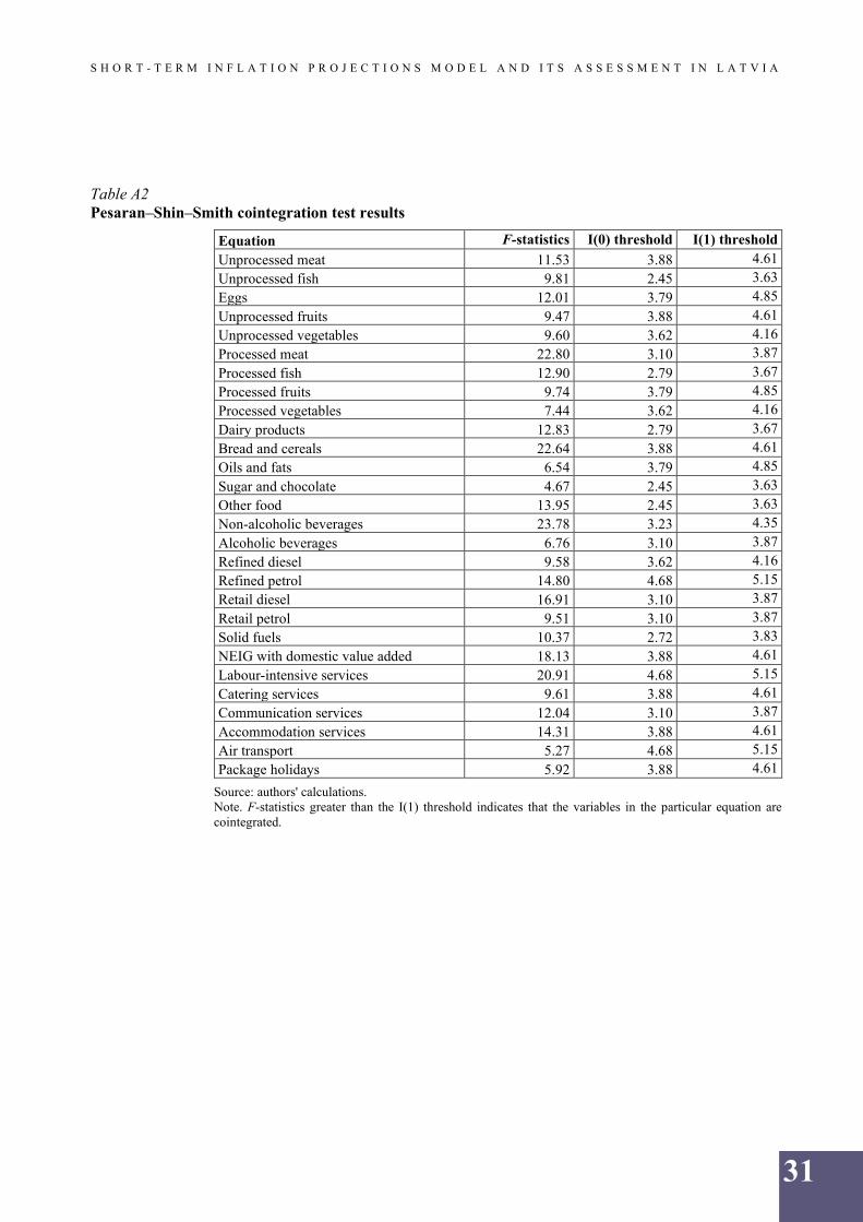
Table A2 Pesaran–Shin–Smith cointegration test results

Equation F-statistics I(0) threshold I(1) threshold Unprocessed meat 11.53 3.88 4.61 Unprocessed fish 9.81 2.45 3.63 Eggs 12.01 3.79 4.85 Unprocessed fruits 9.47 3.88 4.61 Unprocessed vegetables 9.60 3.62 4.16 Processed meat 22.80 3.10 3.87 Processed fish 12.90 2.79 3.67 Processed fruits 9.74 3.79 4.85 Processed vegetables 7.44 3.62 4.16 Dairy products 12.83 2.79 3.67 Bread and cereals 22.64 3.88 4.61 Oils and fats 6.54 3.79 4.85 Sugar and chocolate 4.67 2.45 3.63 Other food 13.95 2.45 3.63 Non-alcoholic beverages 23.78 3.23 4.35 Alcoholic beverages 6.76 3.10 3.87 Refined diesel 9.58 3.62 4.16 Refined petrol 14.80 4.68 5.15 Retail diesel 16.91 3.10 3.87 Retail petrol 9.51 3.10 3.87 Solid fuels 10.37 2.72 3.83 NEIG with domestic value added 18.13 3.88 4.61 Labour-intensive services 20.91 4.68 5.15 Catering services 9.61 3.88 4.61 Communication services 12.04 3.10 3.87 Accommodation services 14.31 3.88 4.61 Air transport 5.27 4.68 5.15 Package holidays 5.92 3.88 4.61

Source: authors' calculations. Note. F-statistics greater than the I(1) threshold indicates that the variables in the particular equation are cointegrated.


32

Table A3 Results of serial correlation and heteroskedasticity tests

Equation Serial correlation test Heteroskedasticity test F-statistics p-value F-statistics p-value

Unprocessed meat 1.50 0.23 0.90 0.50 Unprocessed fish 2.31 0.10 1.57 0.11 Eggs 1.42 0.24 3.34 0.00 Unprocessed fruits 0.06 0.94 0.79 0.64 Unprocessed vegetables 1.12 0.33 1.29 0.28 Processed meat 1.23 0.29 2.01 0.06 Processed fish 0.77 0.46 0.85 0.57 Processed fruits 1.21 0.30 1.07 0.39 Processed vegetables 3.68 0.03 1.16 0.31 Dairy products 1.89 0.15 0.36 0.97 Bread and cereals 0.36 0.70 2.72 0.00 Oils and fats 2.24 0.11 1.50 0.13 Sugar and chocolate 0.42 0.66 1.82 0.09 Other food 0.45 0.64 0.62 0.81 Non-alcoholic beverages 0.13 0.88 1.54 0.10 Alcoholic beverages 1.65 0.20 1.45 0.15 Refined diesel 0.21 0.81 18.85 0.00 Refined petrol 0.53 0.59 1.80 0.07 Retail diesel 1.64 0.19 1.68 0.07 Retail petrol 0.13 0.87 1.78 0.04 Solid fuels 0.79 0.46 1.10 0.37 NEIG with domestic value added 0.78 0.46 1.04 0.41 Labour-intensive services 0.94 0.39 1.14 0.33 Catering services 0.78 0.46 3.66 0.00 Communication services 0.31 0.74 0.98 0.48 Accommodation services 1.87 0.16 0.81 0.72 Air transport 0.44 0.65 4.48 0.00 Package holidays 0.48 0.62 3.72 0.00

Source: authors' calculations. Note. We use the Breusch–Godfrey serial correlation LM test where the null hypothesis states that there is no serial correlation; in the Breusch–Pagan–Godfrey test used for heteroskedasticity, null states homoskedasticity.


33

Table A4 Models' in-sample explanatory power

Equation R2 in levels R2 in differences

Observations

Unprocessed meat 0.9945 0.3376 168 Unprocessed fish 0.9912 0.4211 167 Eggs 0.9895 0.5596 168 Unprocessed fruits 0.9706 0.4846 168 Unprocessed vegetables 0.8253 0.2685 168 Processed meat 0.9965 0.3779 168 Processed fish 0.9988 0.5200 168 Processed fruits 0.9968 0.4321 168 Processed vegetables 0.9542 0.6692 168 Dairy products 0.9980 0.6723 168 Bread and cereals 0.9990 0.7243 167 Oils and fats 0.9974 0.5135 168 Sugar and chocolate 0.9959 0.1650 168 Other food 0.9987 0.4813 167 Non-alcoholic beverages 0.9977 0.5472 167 Alcoholic beverages 0.9956 0.5611 165 Solid fuels 0.9949 0.5844 150 NEIG with domestic value added 0.9983 0.6997 165 Labour-intensive services 0.9997 0.7981 165 Catering services 0.9996 0.8050 163 Communication services 0.9985 0.8127 166 Accommodation services 0.9581 0.8576 168 Air transport 0.9326 0.1213 168 Package holidays 0.9574 0.1577 168 Refined diesel 0.9974 0.8132 732 Refined petrol 0.9908 0.5877 732 Retail diesel 0.9948 0.4520 728 Retail petrol 0.9934 0.5477 729

Source: authors' calculations. Note. A number of observations for refined (retail) diesel and petrol are based on weekly data, for other variables – on a number of monthly observations.


34

Table A5 Error correction coefficients (in descending order)

HICP category Component of HICP Error correction (coefficient)

Number of months when a

shock decreases by half

Energy Retail diesel –0.52 1.3 Energy Refined petrol –0.33 2.1 Energy Retail petrol –0.33 2.1 Unprocessed food Unprocessed vegetables –0.30 2.3 Services Accommodation services –0.28 2.4 Unprocessed food Unprocessed fruits –0.26 2.7 Energy Refined diesel –0.22 3.2 Services Package holidays –0.19 3.7 Processed food Processed meat –0.18 3.8 Services Labour-intensive services –0.14 4.9 Unprocessed food Unprocessed meat –0.13 5.4 Unprocessed food Unprocessed fish –0.12 5.9 Unprocessed food Eggs –0.11 6.1 Processed food Non-alcoholic beverages –0.11 6.1 Services Catering services –0.11 6.4 Processed food Dairy products –0.11 6.5 NEIG NEIG with domestic value added –0.11 6.5 Processed food Bread and cereals –0.09 7.4 Processed food Processed fruits –0.09 8.1 Processed food Processed vegetables –0.08 8.7 Processed food Alcoholic beverages –0.08 9.1 Processed food Other food –0.07 9.3 Processed food Processed fish –0.07 9.5 Energy Solid fuels –0.07 10.5 Processed food Sugar and chocolate –0.06 11.2 Services Air transport –0.06 12.1 Processed food Oils and fats –0.05 15.3 Services Communication services –0.02 39.6

Source: authors' calculations. Note. Error correction coefficients of petrol and diesel were estimated using weekly data and recalculated to monthly equivalent.


35

Table A6 Division of NEIG into those with a considerable domestic value added and other goods

Product category

Component of HICP Weight in the consumption

basket (%)

Coefficient p-value

Goods with domestic value added: Semi-durables Books 0.30 0.36 0.03 Semi-durables Spare parts and accessories for personal transport

equipment 1.02 0.23 0.00 Semi-durables Other personal effects 0.36 0.19 0.01 Semi-durables Glassware, tableware and household utensils 0.51 0.15 0.02 Semi-durables Household textiles 0.22 0.10 0.02 Semi-durables Tools and equipment for house and garden 0.46 0.10 0.03 Non-durables Newspapers and periodicals 0.37 0.30 0.00 Non-durables Materials for the maintenance and repair of the dwelling 0.79 0.25 0.00 Non-durables Other medical products, therapeutic appliances and

equipment 0.31 0.23 0.00 Non-durables Gardens, plants and flowers 0.53 0.22 0.02 Non-durables Products for pets 0.81 0.21 0.01 Non-durables Non-durable household goods 1.10 0.16 0.03 Non-durables Electrical appliances for personal care, other appliances,

articles and products for personal care 1.91 0.16 0.02 Non-durables Miscellaneous printed matter, stationery and drawing

materials 0.26 0.11 0.01 Non-durables Pharmaceutical products 2.94 0.11 0.04 Durables Furniture and furnishings 0.99 0.37 0.00 Durables Jewellery, clocks and watches 0.20 0.15 0.16 Durables Carpets and other floor coverings 0.07 0.07 0.05 Other goods: Semi-durables Games, toys and hobbies 0.44 0.12 0.02 Semi-durables Garments 3.91 0.17 0.00 Semi-durables Recording media 0.09 0.04 0.66 Semi-durables Clothing materials 0.03 0.07 0.38 Semi-durables Shoes and other footwear 1.38 0.14 0.29 Semi-durables Other articles of clothing and clothing accessories 0.29 –0.20 0.15 Semi-durables Equipment for sport, camping and open-air recreation 0.29 –0.24 0.04 Durables Major household appliances whether electric or not and

small electric household appliances 0.74 0.05 0.24 Durables Motor cars 2.12 0.08 0.12 Durables Motorcycles, bicycles and animal drawn vehicles 0.14 0.01 0.93 Durables Photographic and cinematographic equipment and optical

instruments 0.14 –0.05 0.67 Durables Equipment for the reception, recording and reproduction

of sound and picture 0.29 –0.03 0.76 Durables Information processing equipment 0.80 –0.16 0.06 Durables Telephone and telefax equipment 0.22 –0.04 0.72

Sources: CSB data and authors' division. Notes. Coefficients denote elasticity of the NEIG item to wages from regression of the following form: dlog(HICPt) = c1 + c2dlog(wagest−1) + ut where HICPt is individual HICP NEIG items. Regressions are run using quarterly data to capture the fact that a pass-through of wages to prices may take place in different months. P-values relate to the estimated coefficients.


36

Table A7 Components of HICP for services

Product category

Component of HICP Weight in the consumption

basket (%)

Coefficient P-value

Labour-intensive services: Housing Actual rentals for housing 1.06 0.55 0.00 Housing Services for the maintenance and repair of the dwelling 0.62 0.35 0.04 Housing Other services relating to the dwelling n.e.c. 1.90 0.60 0.00 Housing Repair of household appliances 0.02 0.50 0.00 Housing Domestic services and household services 0.22 0.65 0.00 Housing Insurance connected with the dwelling 0.09 0.54 0.00 Miscellaneous Medical and paramedical services 1.24 0.34 0.02 Miscellaneous Dental services 1.14 0.56 0.00 Miscellaneous Financial services n.e.c. 0.28 0.26 0.07 Miscellaneous Other services n.e.c. 0.32 0.75 0.00 Recreation Cleaning, repair and hire of clothing 0.07 0.48 0.00 Recreation Repair and hire of footwear 0.02 0.51 0.00 Recreation Repair of audio-visual, photographic and information

processing equipment 0.11 0.22 0.03 Recreation Veterinary and other services for pets 0.04 0.32 0.00 Recreation Recreational and sporting services 0.68 0.42 0.00 Recreation Cultural services 1.92 0.30 0.00 Recreation Hairdressing salons and personal grooming establishments 0.78 0.45 0.00 Transport Maintenance and repair of personal transport equipment 1.52 0.49 0.00 Transport Other services in respect of personal transport equipment 0.68 0.68 0.00 Transport Passenger transport by sea and inland waterway 0.14 0.76 0.08 Transport Insurance connected with transport 0.66 0.61 0.01 Other services: Communication Telephone and telefax services 3.13 –0.05 0.42 Recreation Catering services 5.56 0.42 0.00 Recreation Accommodation services 1.80 0.20 0.27 Recreation Package holidays 0.66 0.56 0.00 Transport Passenger transport by air 0.82 0.17 0.36 Administered services: Communication Postal services 0.03 –0.07 0.83 Housing Refuse collection 0.52 0.42 0.01 Housing Sewerage collection 0.52 0.57 0.00 Miscellaneous Hospital services 0.39 –0.46 0.25 Miscellaneous Social protection 0.29 0.17 0.12 Transport Passenger transport by railway 0.52 0.45 0.01 Transport Passenger transport by road 2.07 0.32 0.01

Sources: CSB data and authors' division. Notes. Coefficients denote elasticity of the services item to wages from regression of the following form: dlog(HICPt) = c1 + c2dlog(wagest−1) + ut where the HICP is services items. Regressions are run using quarterly data to capture the fact that a pass-through of wages to prices may take place in different months. P-values relate to the estimated coefficients.


37

Table A8 Pass-through of a 10% increase in labour costs to consumer prices after three years (%)

Impact of a 10% wage increase on consumer prices

Weight in the consumer

basket after 1 year after 3 years HICP 2.40 3.14 100.0 Services 4.58 5.32 31.1 Labour-intensive services 6.98 7.60 13.5 Catering services 6.53 7.77 5.6 Package holidays 4.54 5.01 0.7 Accommodation services 1.02 0.99 1.8 Communication services 1.80 4.10 3.1 Air transport 0.21 0.45 0.8 Industrial goods 0.77 1.40 24.7 of which: with domestic value added 1.44 2.64 13.1 Food products 2.03 3.06 29.6 Unprocessed food products 4.23 4.84 5.3 Unprocessed meat 3.88 4.78 2.1 Unprocessed fish 1.49 3.22 0.2 Eggs 3.19 4.43 0.6 Unprocessed fruits 5.64 5.66 1.0 Unprocessed vegetables 4.59 4.67 1.3 Processed food products 1.78 3.05 21.3 Processed meat 2.77 4.18 2.5 Processed fish 1.71 2.76 0.7 Processed fruits 3.93 6.21 0.2 Processed vegetables 1.80 2.80 0.6 Dairy products 3.08 3.49 3.4 Bread and cereals 3.57 6.45 3.7 Oils and fats 2.07 3.46 1.0 Sugar and chocolate 2.51 3.78 1.7 Other food products 1.54 2.85 0.7 Non-alcoholic beverages 0.75 1.62 1.8 Alcoholic beverages 0.05 1.60 4.9 Energy 0.32 0.35 14.5 Car fuel 0.79 0.87 5.9

Source: authors' calculations based on CSB data.


38

Table A9 Relative forecast errors of individual components

HICP item

3 months ahead

6 months ahead

12 months ahead

Unprocessed food: Meat 0.85 0.75 0.56 Fish 0.75 0.69 0.57 Eggs 0.99 1.03 1.05 Fruits 0.89 0.96 0.74 Vegetables 0.81 0.80 0.68 Processed food: Meat 0.93 0.88 0.74 Fish 1.10 1.10 0.94 Fruits 0.94 0.92 0.84 Vegetables 0.91 0.96 1.05 Dairy 0.87 0.81 0.73 Cereals 0.82 0.61 0.44 Oils 0.94 0.95 0.96 Sugar 0.98 0.90 0.94 Other food 1.10 1.07 0.96 Non-alcoholic beverages 0.88 0.83 1.07 Alcoholic beverages 0.89 0.84 0.68 NEIG: With domestic value added 0.71 0.54 0.35 Services: Labour-intensive services 1.11 1.01 0.99 Catering services 1.29 1.02 0.59 Communication 0.68 0.57 0.51 Accommodation 0.88 0.84 0.67 Air transport 0.96 0.94 0.89 Package holidays 0.86 0.81 0.67 Energy: Car fuel 0.91 0.86 0.82

Source: authors' calculations. Notes. The table shows RMSFEs of the STIP model relative to the RMSFEs of the random walk at horizons of 3, 6 and 12 months ahead. Tobacco, other NEIG, water supply and administered services are forecasted as random walk. Solid fuel prices are also modelled as random walk in this forecast evaluation exercise, because we lack real-time assumptions of timber prices since 2014. In turn, education prices, natural gas, electricity and heat energy are unchanged over the forecast horizon (flat). Therefore, forecast errors of these components are not shown here.


39

Figure A1 Consumer prices of unprocessed food components (index: 2015 = 100)

Source: CSB data.


40

Figure A2 Consumer prices of processed food components (index: 2015 = 100)


41

Source: CSB data.

Figure A3 Decomposition of petrol prices (euro per litre)

Sources: Bloomberg, EC and CSB data and authors' calculations.

Figure A4 Consumer prices of industrial goods in Latvia by product group (index: 2015 = 100)

Source: Eurostat data.


42

Figure A5 Consumer prices of selected durable industrial goods in Latvia (index: 2015 = 100)

Sources: CSB data and authors' calculations.

Figure A6 Share of imports in NEIG consumption (%)

Sources: CSB and Eurostat data and authors' calculations. Note. Estimates exclude passenger cars and re-exports.


43

Figure A7 Relation between domestic economic activity indicators and consumer prices of industrial goods (%)

Economic growth and consumer price inflation of industrial goods in the EU countries

(by country; annual average over 2000–2018)

Average wage growth and consumer price inflation of industrial goods in Latvia (by year over 2000–2018)

Sources: CSB and Eurostat data and authors' calculations. Note. The figure on the left excludes Ireland as outlier; the figure on the right excludes the years 2009 and 2010.


44

Figure A8 Consumer prices of services (index: 2015 = 100)

Source: CSB data.


45

Figure A9 Air transport prices in the EU countries (%; cumulative change over 2015–2018)

Sources: Eurostat data and authors' calculations.


46

Figure A10 Administered prices (index: 2015 = 100)

Source: CSB data.


47

Figure A11 Monthly changes of education services prices

Source: CSB data.

Figure A12 Pass-through of a 10% increase in the global food commodity prices to consumer prices of food products in Latvia (%)

Sources: authors' calculations based on EC and CSB data. Notes. Estimates are made over the 2005–2018 period using monthly data; the simulation assumes a 10% increase in global price of food commodities starting in January 2019. The red line shows the average and the bands show a 68% confidence interval.


48

Figure A13 Pass-through of a 10% increase in labour costs to consumer prices of selected services, industrial goods and food products in Latvia (%)

Sources: authors' calculations using EC and CSB data. Notes. Estimates are made over the 2005–2018 period using monthly data; the simulation assumes a permanent average wage rise by 10% as from January 2019. The red line shows the average and the bands show a 68% confidence interval.


49

Figure A14 Relationship between domestic economic activity indicators and consumer prices of services (%)


Figure A15 Average monthly gross wage (blue) and consumer prices of selected services in Latvia (orange; right axis)


50



51

Figure A16 Relationship between domestic economic activity and consumer food prices (%)

Economic growth and consumer food price inflation in the EU countries (by country; annual average over 2000–2018)

Average wage growth and consumer food price inflation in Latvia (by year over 2000–2018)



52

Figure A17 Average monthly gross wage (euro; blue) and the difference between consumer prices of selected food products in Latvia and corresponding food commodity producer price in the EU (orange; right axis)



53

BIBLIOGRAPHY

ÁLVAREZ, Luis J., SÁNCHEZ, Isabel (2017). A Suite of Inflation Forecasting Models. Banco de España Occasional Paper, No. 1703. 52 p.

ARON, Janine, MUELLBAUER, John (2012). Improving Forecasting in an Emerging Economy, South Africa: Changing Trends, Long Run Restrictions and Disaggregation. International Journal of Forecasting, Elsevier, vol. 28, issue 2, pp. 456–476.

ARON, Janine, MUELLBAUER, John (2013). New Methods for Forecasting Inflation, Applied to the US. Oxford Bulletin of Economics and Statistics, Department of Economics, University of Oxford, vol. 75, issue 5, October 2013, pp. 637–661.

BANBURA, Marta, GIANNONE, Domenico, REICHLIN, Lucrezia (2010). Large Bayesian Vector Auto Regressions. Journal of Applied Econometrics, vol. 25, issue 1, pp. 71–92.

BENALAL, Nicholai, DEL HOYO, Juan Luis Diaz, LANDAU, Bettina, ROMA, Moreno, SKUDELNY, Frauke (2004). To Aggregate or Not to Aggregate? Euro Area Inflation Forecasting. ECB Working Paper, No. 374, July 2004. 65 p.

BERMINGHAM, Colin, D'AGOSTINO, Antonello (2014). Understanding and Forecasting Aggregate and Disaggregate Price Dynamics. Empirical Economics, Springer, vol. 46, issue 2, March 2014, pp. 765–788.

BOIVIN, Jean, NG, Serena (2005). Understanding and Comparing Factor-Based Forecasts. International Journal of Central Banking, vol. 1, No. 3, December 2005, pp. 117–151.

BRUNEAU, Catherine, DE BANDT, Olivier, FLAGEOLLET, Alexis, MICHAUX, Emmanuel (2007). Forecasting Inflation Using Economic Indicators: The Case of France. Journal of Forecasting, John Wiley & Sons, Ltd., vol. 26, issue 1, pp. 1–22.

CLARK, Todd E., WEST, Kenneth D. (2007). Approximately Normal Tests for Equal Predictive Accuracy in Nested Models. Journal of Econometrics, Elsevier, vol. 138, issue 1, pp. 291–311.

DEN REIJER, Ard, VLAAR, Peter (2006). Forecasting Inflation: An Art as Well as a Science! De Economist, Springer, vol. 154, issue 1, March 2006, pp. 19–40.

DUARTE, Cláudia Filipa, RUA, António (2007). Forecasting Inflation through a Bottom-up Approach: How Bottom Is Bottom? Economic Modelling, vol. 24, issue 6, November 2007, pp. 941–953.

ESPASA, Antoni, ALBACETE, Rebeca (2007). Econometric Modelling for Short-Term Inflation Forecasting in the EMU. Journal of Forecasting, John Wiley & Sons, Ltd., vol. 26, issue 5, pp. 303–316.

ESPASA, Antoni, PONCELA, Pilar, SENRA, Eva (2002a). Forecasting Monthly US Consumer Price Indexes through a Disaggregated I(2) Analysis. Universidad Carlos III de Madrid, Departamento de Estadística y Econometría. Statistics and Econometrics Series 01, Working Paper 02-03, January 2002. 28 p.


54

ESPASA, Antoni, SENRA, Eva, ALBACETE, Rebeca (2002b). Forecasting Inflation in the European Monetary Union: A Disaggregated Approach by Countries and by Sectors. The European Journal of Finance, vol. 8, issue 4, pp. 402–421.

ECB (2010). Tools for Preparing Short-Term Projections of Euro Area Inflation. Monthly Bulletin, April 2010, pp. 65–73.

ECB (2016). A Guide to the Eurosystem/ECB Staff Macroeconomic Projection Exercises. July 2016. 36 p.

FERRUCCI, Gianluigi, JIMÉNEZ-RODRÍGUEZ, Rebeca, ONORANTE, Luca (2012). Food Price Pass-Through in the Euro Area: Non-Linearities and the Role of the Common Agricultural Policy. International Journal of Central Banking, vol. 8, issue 1, March 2012, pp. 179–218.

FRITZER, Friedrich, MOSER, Gabriel, SCHARLER, Johann (2002). Forecasting Austrian HICP and Its Components Using VAR and ARIMA Models. Oesterreichische Nationalbank Working Paper, No. 73, August 2002. 37 p.

GIANNONE, Domenico, LENZA, Michele, MOMFERATOU, Daphne, ONORANTE, Luca (2014). Short-Term Inflation Projections: A Bayesian Vector Autoregressive Approach. International Journal of Forecasting, Elsevier, vol. 30, issue 3, pp. 635–644.

HARVEY, David, LEYBOURNE, Stephen, NEWBOLD, Paul (1997). Testing the Equality of Prediction Mean Squared Errors. International Journal of Forecasting, Elsevier, vol. 13, issue 2, June 1997, pp. 281–291.

HENDRY, David Forbes, HUBRICH, Kirstin (2011). Combining Disaggregate Forecasts or Combining Disaggregate Information to Forecast an Aggregate. Journal of Business and Economic Statistics, vol. 29, issue 2, April 2011, pp. 216–227.

HUBRICH, Kirstin (2005). Forecasting Euro Area Inflation: Does Aggregating Forecasts by HICP Component Improve Forecast Accuracy? International Journal of Forecasting, Elsevier, vol. 21, issue 1, pp. 119–136.

HUWILER, Marco, KAUFMANN, Daniel (2013). Combining Disaggregate Forecasts for Inflation: The SNB's ARIMA Model. Swiss National Bank Economic Studies, No. 2013-07. 30 p.

LÜTKEPOHL, Helmut (1984a). Forecasting Contemporaneously Aggregated Vector ARMA Processes. Journal of Business and Economic Statistics, vol. 2, issue 3, pp. 201–214.

LÜTKEPOHL, Helmut (1984b). Linear Transformations of Vector ARMA Processes. Journal of Econometrics, vol. 26, issue 3, pp. 283–293.

LÜTKEPOHL, Helmut (1987). Forecasting Aggregated Vector ARMA Processes. Berlin: Springer-Verlag. 323 p.

MARCELLINO, Massimiliano, STOCK, James H., WATSON, Mark W. (2003). Macroeconomic Forecasting in the Euro Area: Country Specific versus Area-Wide Information. European Economic Review, Elsevier, vol. 47, issue 1, February 2003, pp. 1–18.


55

MARCELLINO, Massimiliano, STOCK, James H., WATSON, Mark W. (2006). A Comparison of Direct and Iterated Multistep AR Methods for Forecasting Macroeconomic Time Series. Journal of Econometrics, Elsevier, vol. 135, pp. 499–526.

MEYLER, Aidan (2009). The Pass Through of Oil Prices into Euro Area Consumer Liquid Fuel Prices in an Environment of High and Volatile Oil Prices. Energy Economics, Elsevier, vol. 31, issue 6, November 2009, pp. 867–881.

MOSER Gabriel, RUMLER, Fabio, SCHARLER, Johann (2007). Forecasting Austrian Inflation. Economic Modelling, Elsevier, vol. 24, issue 3, May 2007, pp. 470–480.

PEACH, Richard W., RICH, Robert W., ANTONIADES, Alex (2004). The Historical and Recent Behaviour of Goods and Services Inflation. Economic Policy Review, Federal Reserve Bank of New York, December 2004, pp. 19–31.

PEERSMAN, Gert (2018). International Food Commodity Prices and Missing (Dis)Inflation in the Euro Area. Center for Economic Studies and Ifo Institute (CESifo), CESifo Working Paper, No. 7338, November 2018. 43 p.

PESARAN, M. Hashem, SHIN, Yongcheol (1998). An Autoregressive Distributed-Lag Modelling Approach to Cointegration Analysis. Econometric Society Monographs, vol. 31, pp. 371–413.

PESARAN, M. Hashem, SHIN, Yongcheol, SMITH, Richard J. (2001). Bounds Testing Approaches to the Analysis of Level Relationships. Journal of Applied Econometrics, John Wiley & Sons, Ltd., vol. 16, issue 3, pp. 289–326.

PUFNIK, Andreja, KUNOVAC, Davor (2006). Short-Term Forecasting of Inflation in Croatia with Seasonal ARIMA Processes. Croatian National Bank Working Paper, No. 16, December 2006. 19 p.

STAKĖNAS, Julius (2015). Forecasting Lithuanian Inflation. Bank of Lithuania Working Paper, No. 17. 42 p.

STOCK, James H., WATSON, Mark W. (1999). Forecasting Inflation. Journal of Monetary Economics, Elsevier, vol. 44, issue 2, October 1999, pp. 293–335.

STOCK, James H., WATSON, Mark W. (2002). Forecasting Using Principal Components from a Large Number of Predictors. Journal of the American Statistical Association, vol. 97, pp. 1167–1179.

Date post:	16-Jan-2022
Category:	Documents
Upload:	others
View:	3 times
Download:	0 times

ANDREJS BESSONOVS OĻEGS KRASNOPJOROVS 1 / 2020

Documents