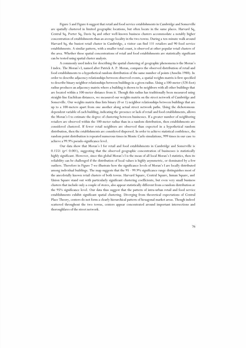
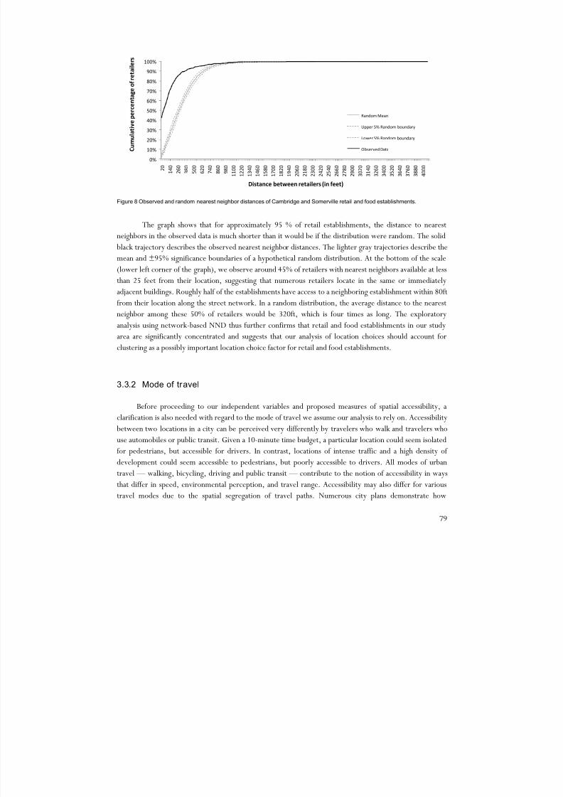
PhD DISSERTATION MASSACHUSETTS INSTITUTE OF TECHNOLOGY Department of Urban Studies & Planning Title: Path and Place: A Study of Urban Geometry and Retail Activity in Cambridge and Somerville, MA. PhD Candidate: Andres Sevtsuk City Design & Development / Urban Information Systems Dissertation Committee: William C. Wheaton Professor of Economics, MIT Director of Research, Center for Real Estate at MIT John P. De Monchaux Professor of Architecture and Planning Emeritus, MIT Philip Steadman Professor of Urban & Built Forms Studies University College London (UCL) William J. Mitchell (1944 – 2010) Professor of Architecture and Media Arts & Sciences Director of Smart Cities Group, MIT Media Laboratory Date: August 11, 2010 This dissertation was made possible by the generous support of the Government of Portugal through the Portuguese Foundation for International Cooperation in Science, Technology and Hi gher Education and was undertaken in the MIT-Portugal Program.
MASSACHUSETTS INSTITUTE OF TECHNOLOGYDepartment of Urban Studies & Planning
Title: Path and Place: A Study of Urban Geometry and Retail Activity inCambridge and Somerville, MA.
PhD Candidate: Andres SevtsukCity Design & Development / Urban Information Systems
Dissertation Committee: William C. WheatonProfessor of Economics, MITDirector of Research, Center for Real Estate at MIT
John P. De MonchauxProfessor of Architecture and Planning Emeritus, MIT
Philip SteadmanProfessor of Urban & Built Forms StudiesUniversity College London (UCL)
William J. Mitchell (1944 – 2010)Professor of Architecture and Media Arts & SciencesDirector of Smart Cities Group, MIT Media Laboratory
Date: August 11, 2010
This dissertation was made possible by the generous support of the Government of Portugal through thePortuguese Foundation for International Cooperation in Science, Technology and Higher Education and wasundertaken in the MIT-Portugal Program.
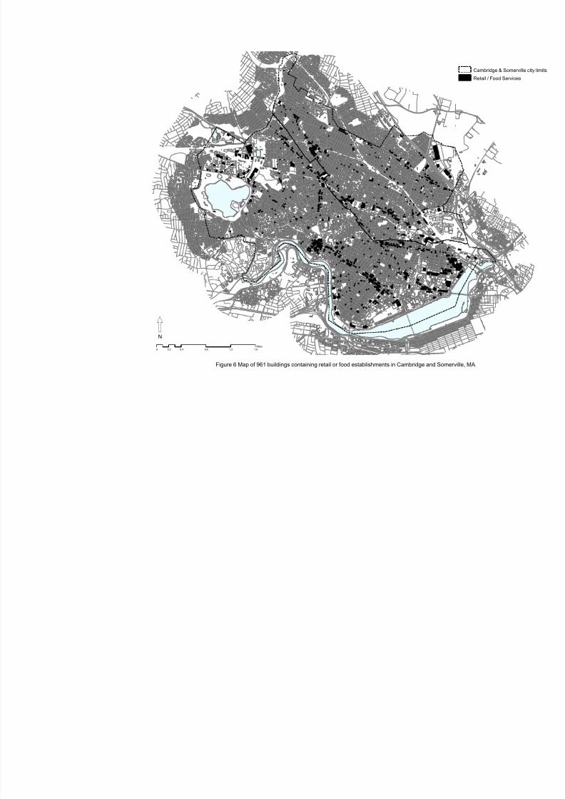
This dissertation investigates retail location patterns in urban settings – a domain that has received
relatively little attention in recent decades. We analyze which land use, urban form, and agglomeration
factors explain observed retail patterns in an empirical case study of Cambridge and Somerville, MA. We
are particularly interested in whether and how the distribution of retailers is affected by the spatial
configuration of the built environment – the physical pattern of urban infrastructure, the spacing and sizes
of buildings, and the geometry of circulation routes. We argue that understanding retail location patterns in
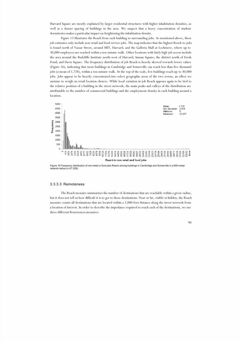
urban settings is not only important for improving retail location theory, but also essential for designing
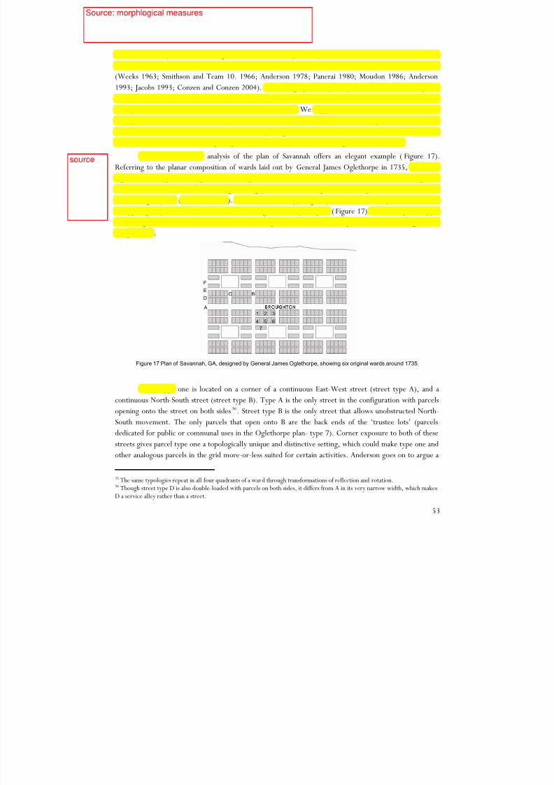
economically, socially, and environmentally sustainable urban neighborhoods.
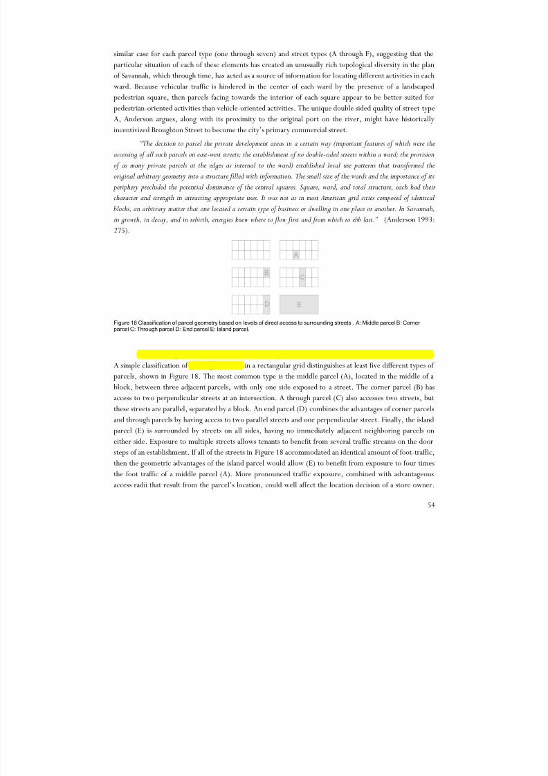
The dissertation proposes a novel graph-analysis framework in which retail location patterns can berepresented under realistic constraints of urban geometry, land use distribution, and travel behavior. A
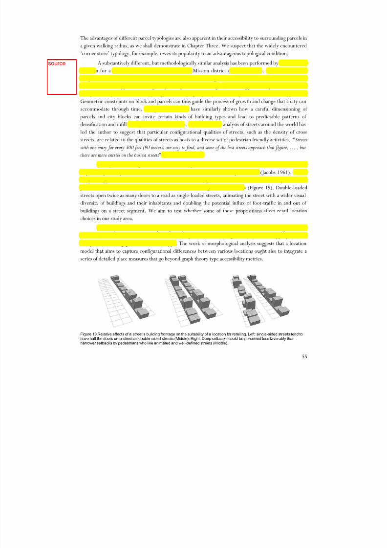
series of spatial accessibility metrics, which we hypothesize to affect retail location choices, are introduced
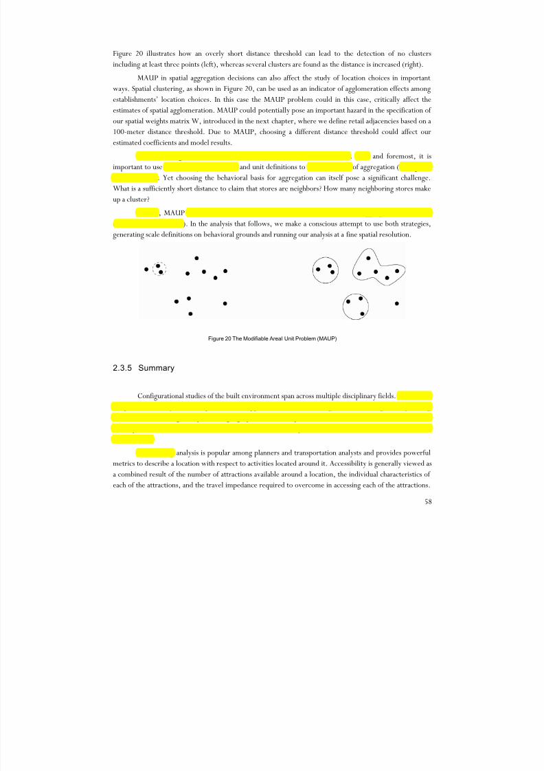
and applied in this framework using individual buildings as units of analysis. In order to test the statistical
significance of these different metrics on retail location choices, we adopt the strategic interaction
methodology from spatial econometrics and apply it for the first time in the context of location studies. We
specify a linear probability model with a binary dependent variable and estimate how buildings’ probabilities
to accommodate retail establishments relate endogenously to other retailers’ location choices and
exogenously to both land use and urban form characteristics around each building. We apply the model to
all retail and food-service establishments as a group and to different three-digit NAICS establishment
categories individually.
The results confirm that retail location choices in our study area are significantly related to both
other retailers’ endogenous location choices and exogenous land use characteristics around each building.
However, controlling for both of these factors, we find that the spatial distribution of retail activity is also
significantly related to the geometry of the built environment. By setting constraints on accessibility,
visibility, adjacency, and density, the geometry of the built environment produces a rich landscape of
information that appears to guide opportunities for business from building to building.
The findings inform economists and planners about factors that attract retailers in urban settings,
and urban designers about how the seemingly basic act of laying out streets, parcels and buildings can affect
the location choices retail and service land uses, thereby shaping the economic structure of the city inimportant ways.
This dissertation talks about the importance of physical places, but it is also itself very much a
product of an extraordinary place — MIT. The brilliant people, ideas, and opportunities connected through
a web of infinite paths around this Institute have played a central role in the development of this research.
The idea to study the influence of urban geometry on land use locations choices using both retail location
theory and configurational studies of the built environment is probably partly due to the close spatial
connectivity between the various departments of this campus. But it is undoubtedly the gifted faculty and
colleagues around the Institute who have helped me grow this idea into a dissertation.
I am particularly grateful to my dissertation committee, who has guided me to areas of inquiry that
I would have otherwise not found, and kept me away from others that I would probably have stumbled intowithout them. Bill Wheaton has not only inspired me to look into fascinating areas of spatial econometrics
and land use location theory, but also guided the development of the entire analysis and kept me in tune
with the relevant literature on the economics side. John de Monchaux has been a continuous source of
inspiration for thinking about urban geometry and the origins thereof. John’s love and knowledge of cities
have taught me to study the built environment with great respect as well as a critical eye. Philip Steadman,
who joined the committee from the Bartlett Faculty in London, brought an invaluable perspective for
measuring and describing the built environment with rigor, and anchored this research in a long tradition of
built form studies in Europe and beyond. And finally Bill Mitchell — my long-term advisor and mentor, as
well as the chair of this committee until his very unfortunate departure — was one of the most creative
thinkers I have ever encountered, an immense source of inspiration both intellectually and personally. Much
of his advice is embedded in this dissertation.
I am also grateful for the advice of numerous colleagues, friends, and mentors beyond the
dissertation committee: Julian Beinart, Suzanne de Monchaux, Frank Levy, Dennis Frenchman, Chris
Zegras, Eran Ben-Joseph, Duncan Kincaid, Ray Huling and Noah Raford among others.
I am sincerely thankful to my parents and my brother’s family for their continuous support and love
over the years, and to Lily’s family in LA for their warmth and love. My deepest gratitude goes to Lily, my
partner in life and closest friend, for sharing with me the hours, weeks, and years, with or without this
Understanding the relationship between the spatial structure of human settlements and the social life
of their inhabitants is one of the central challenges of city planning. Yet despite extensive investigation to
date, the relationship between the spatial configuration of cities and social processes that take place in them
has proven to be a topic of extraordinary complexity, with only modest advances available to illuminate a
dissertation on the matter. The importance of built geometry in the ancient monastic societies of the
Middle- and Far-East, and South America went beyond symbolic significance, affecting numerous
procedures of daily life (Lynch 1984). Studies of indigenous cultures in the American Amazon have
suggested that the geometry of settlement patterns was of vital importance in preserving social organization
and kinship hierarchies (Lévi-Strauss 1963). There is little consensus, however, over the significance ofurban form in contemporary societies.
Making reference to life sciences, Jane Jacobs has described cities as problems of organized
complexity , which not only contain a large number of variables, but also challenge an analyst with countless
interrelationships between the variables (Jacobs 1961: 428). Indeed, the state of knowledge of the form-
process dialectic suggests that general questions such as ‘what is the influence of urban configuration on
social life?’ are defeated at the outset, since more interactions are found than a single answer could possibly
suggest. Perhaps more important, the notion of complexity evoked in Jacobs’ reading of cities, also suggests
that any particular interaction between form and use is likely to be neither unique nor deterministic.
Instead, the argument suggests, the relationship can take many forms and depend on a range of additionalfactors that affect people’s use of space beyond spatial form. Using an example of city parks, Jacobs argues:
“How much a park is used depends, in part, upon the park’s own design. But even this partial influence of the park’s
design upon the park’s use depends, in turn, on who is around to use the park, and when, and this in turn depends on the
uses of the city outside the park itself. Furthermore, the influence of these uses on the park is only partly a matter of how
each affects the park independently of the others; it is also partly a matter of how they affect the park in combination
with one another, for certain combinations stimulate the degree of the influence from one another among their
components… No matter what you try to do to it, a city park behaves as a problem in organized complexity, and that is
what it is. ” (Jacobs 1961: 433)
Jacobs’ remarks came at a time when architectural intervention was still widely regarded as theprimary tool for addressing the social and economic ills of cities. Jacobs invited architects to investigate the
complex interaction between form and use and cautioned designers and policy makers to recognize the
limits of spatial design and to refrain from inferring strong causal relationships without the support of
evidence.
Vigilant against ‘spatial determinism’, a number of urban sociologists have drawn a similar critique,
alerting urban designers to remain wary of what Webber has called “some deep-seated doctrine that seeks order in
some simple mappable patterns, when it is really hiding in extremely complex social organization instead “ (Webber
1963). These arguments developed largely in response to a series of large-scale urban renewal projects
across the U.S. and Europe that had addressed acute poverty in distressed urban areas using urban design as
the primary tool. These projects produced disastrous consequences. Though it can be argued that these
consequences were the result of a limited social and economic scope of the interventions, the critique also
pointed out the insufficiency of a historic and deeply-rooted tradition of city planning that, until then, had
been principally dominated by architects (Howard 1902; Garnier 1939; LeCorbusier 1967; Fourier 1971),
and which had come to exhibit its limits in dealing with complex social and economic problems in postwar
cities. The critics contended that a deeper understanding of the relationship between spatial and social
processes was needed before urban design could be taken as a fix to any of the latter.
While it is now generally accepted that urban design is not the only — nor by any means the
dominant — force acting upon the social life of cities, urban designers’ response to the Webberian criticism
has proven difficult and slow. This shortcoming has gradually pushed the field of urban design towards themargins of the contemporary theory of urban studies and planning. Within these confines, important
theoretical developments in urban design have indeed occurred. Neo-Marxist planning theory, for instance,
has offered a view of urban development that acknowledges the diverse actors and institutions affecting the
spatial structure of cities, in which urban design holds a modest but important position (Harvey 1973;
Lefebvre 1974; Gottdiener 1985). Christopher Alexander, Leslie Martin, Kevin Lynch, John Habraken,
Konstantinos Doxiadis, and others have searched vigorously for plausible propositions that would link
physical configuration with the qualities of cities (Alexander 1964; Doxiades 1968; Martin and March 1972;
Lynch 1984; Habraken and Teicher 1998). Yet skepticism and pressure still loom over urban design
scholars, whose theoretical foundations for the social value of spatial design still remain fragile. “Maybe Team
X and Archigram”, writes Koolhaas, “were, in the sixties, the last real ‘movements’ in urbanism, the last ones to
propose with conviction new ideas and concepts for the organization of urban life” (Koolhaas 2001).
The general view of urban design within the larger field of city planning today has come to the
point where it is no longer a question of whether there are additional influences on social behavior beyond
spatial configuration, as an 18th- or 19th-century architect might have conceded, but rather if spatial
configuration has any importance at all for the social processes of the city (Talen and Ellis 2002). This
dissertation is largely motivated by a conviction that this view is problematic on several fronts. First, as a
growing proportion of human activities take place in cities (UnitedNations 2007), it becomes increasingly
important to understand how the physical environment of the city affects, and desirably benefits, the
activities of its users. Most daily activities of city dwellers are constrained, to a greater or lesser degree, by
the configuration of the built environment — the physical pattern of urban infrastructure, the geometry of
built form and its circulation routes, the shape of public space and paths that connect them. The basic social
significance of urban form thus emerges through the mere fact of its ubiquitous use. The growth and change
of cities at an unprecedented rate demands attention to form and more empirical research, not neglect. The
consequences of disregarding spatial configuration and geometry in the contemporary planning of cities
could be as grave as their excessive emphasis in the mid-century urban renewals.
Second, despite the inadequacy of professional knowledge concerning the ingredients of ‘good city
form’, a layperson’s attraction towards delightful urban environments, such as Paris, Porto, or Hong Kong,
provides testimony to the important role that urban geometry plays in shaping our attitudes towards cities.
Rather than assigning the emotions triggered by delightful urban environments to the realm of the
metaphysical, we might attempt to understand them with methodological rigor. Learning from precedent isof course a central component of a designer’s education, but the attempts to capture the positive qualities of
past precedents often seem to lead to mimicry and kitsch, instead of constructive knowledge for intelligent,
context-appropriate design. In order to venture towards a better understanding of the social significance of
environmental geometry, precedents need to be examined not only through plans, but also through
observation, user accounts, and other forms of social, economic, and environmental data.
Third, important developments in configurational studies have occurred since the writing of Lynch
and others, creating new opportunities for empirical research on city form. Among these, the ubiquity of
computers and the availability of data that describe both static and dynamic components of the city have
dramatically improved an analyst’s capacity to study complex relationships between built form and its
occupancy patterns. Tools like geographic information systems (GIS), computer-aided design (CAD),
digital databases, and statistical software, largely unavailable a decade ago, have now become widely
available to urban designers. Furthermore, geographically-referenced digital data describing the built,
social, and economic environment of the city have become accessible for research during the same period.
These developments have opened up various new directions for theoretical and empirical propositions
about city form and initiated an active area of urban design research1.
Taking advantage of some of these developments, this dissertation introduces an alternative view of
urban design than architects would typically express. It focuses on a configurational view of urban design —
the study of how the geometric layout of streets, parcels, and buildings can affect the perceived value and
patterns of use of different locations within a city. Rather than centering on the qualities of buildings andstreets themselves, this dissertation focuses predominantly on the spatial interdependence between these
elements of the city. This view of urban design under emphasizes many important sensory characteristics of
1 The contemporary centers of research include the Santa Fe Institute, the Center of Advanced Spatial Analysis (CASA) and the
Space Syntax group in London, the Human Space Lab in Milan, the UPC Barcelona, l’Institut Français d’Urbanisme, and the city
design and development and urban information systems groups at MIT, to name a few.
the built environment that contribute to our daily appreciation of cities — the identity, the aesthetic
quality, and the meaning of buildings, streets, and public spaces. In fact, in the following analysis, we alter
our field of vision so that we may perceive the invisible aspects of city design that cannot be seen through
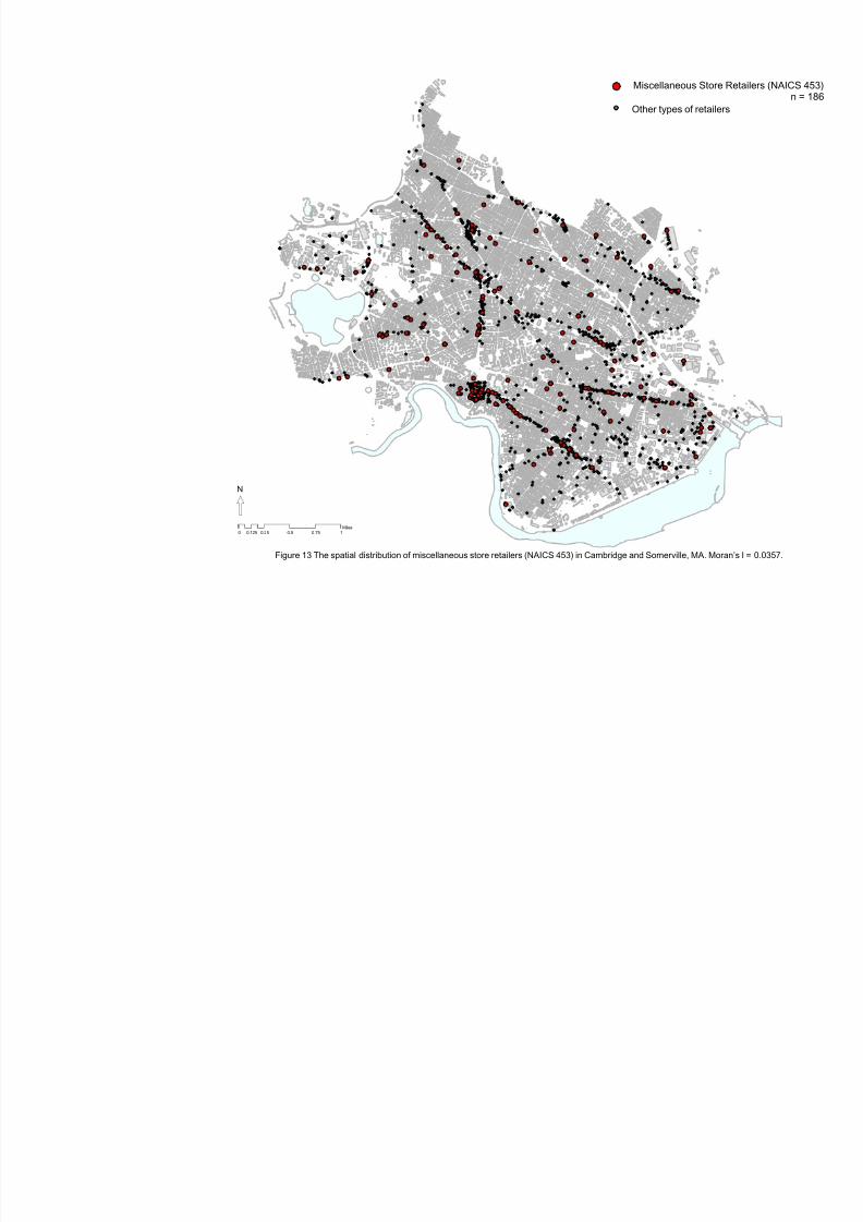
the eyes of an observer at any single location in the city. Instead, we attempt to capture the dynamics that
emerge as people travel through streets, moving from one building to another, collectively producing the
patterns of flow and encounter that make different locations within the network of city streets more or less
amenable for different activities. In this respect, some might argue that this study does not even deal with
urban design or architecture, since “Architecture begins where engineering ends”, as Walter Gropius said.
Yet the practice of urban design shows that the functional prerequisites that good architecture relies upon
are poorly attended to in practice and insufficiently addressed in academia. Compared to the capacity to
produce individual buildings of architectural quality, contemporary urbanism appears less able to capitalize
on what Jan Gehl calls the life between buildings2: the social and economic linkages and movement patterns
that result from inter-relationships between buildings and which each building in turn contributes to. Even
the most outstanding individual buildings or public spaces can fail to be appropriated by their users if the
spatial configuration around the projects disincentivizes their workings
3
. We shall thus argue that, despitethe narrow focus that a configurational view of urban design offers, the spatial configuration of the built
environment can produce important effects for the social use of buildings — effects, which may at times
outweigh the sensory qualities of buildings and public spaces themselves. In the long run, a better
understanding of the configurational qualities of place may also lead us to a better understanding of the
fundamental interactions that link qualities of urban structure to the qualities of meaning and identity in
architecture (Lynch 1996: 252).
Research on different aspects of the social significance of urban form has not only been criticized
outside of the urban design field, but also within. It is often urban designers, architects, and planners
themselves who dispute the existence of any systematic relationships between spatial and social structure.
Claims towards such a relationship appear to challenge a deep-rooted conviction that the creative human
agency that guides city development makes each piece of a city so unique as to render any systematic
analysis meaningless. Even if systematic relationships are found, the critics argue, they have limited value in
normative situations because creativity and unorthodox solutions can always displace historic conventions of
development. Researching the relationship between spatial form and social behavior thus appears to
challenge the agency of a designer. This sort of criticism stems from a perceived difference between
practical knowledge (Schön 1983), embodied in a designer on the one hand, and codifiable and explicit
knowledge that is produced in research, on the other. We do not challenge the central importance of
implicit practical knowledge or Metis, a Greek term derived from the Goddess of the same name who
personified wisdom (Scott 1999), in the design process. Rather, the spatial research developed in thisdissertation explores how research findings, obtained by analyzing large amounts of data, could supplement
the diverse arsenal of knowledge used by design professionals in practice. Beyond practical applicability,
2 See Gehl, J. (1987). Life between buildings : using public space. New York, Van Nostrand Reinhold.
3 One of many well-known examples is the Constitution Plaza in Hartford, CT by another modernist designer Victor Gruen.
however, we also remain hopeful that a stronger appreciation for research might help the field of urban
design reclaim its theoretical position in the larger field of urban studies and planning.
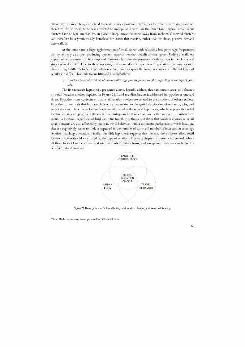
1.2 Statement of the problem
This dissertation focuses on a particular aspect of the urban form-process relationship. The social
process we examine is the choice of location for operating one’s business in an urban environment. The
central question of the dissertation is the following: Does the spatial configuration of the built environment affect
location choices of retail and food service establishments?
By ‘spatial configuration’ we refer to the relationships of adjacency and connectivity that result
from the geometric layout of buildings and public spaces and the circulation routes that connect them. We
are interested in exploring whether the spatial patterns of access and encounter that result from the
particular way these elements of the city are laid out may generate economic incentives for locating one’s
business in one location rather than another. Put alternatively, we investigate whether physical design issignificantly related to the distribution of retail activities in a city. Confirming a plausible relationship with
evidence could shed new light on the social significance of urban design, a topic that remains widely
disputed in mainstream planning theory. The findings could also lead to practically valuable knowledge
regarding the effects of urban form on location and land use.
The relationship between retail location choices and the spatial configuration of a city has been
subject to some study, but a good deal more assertion. New Urbanists’ claims, among others, about the
importance of density and accessibility for sustaining retail and service establishments in town centers have
produced surprisingly little empirical research (Duany, Plater-Zyberk et al. 1991). Scholars using graph
theory metrics on urban form, on the other hand, have produced numerous studies on the subject, but
shortcomings in methodological rigor have rendered their results too porous to be taken seriously in the
planning and economic research community (Hillier 1996; Porta, Crucitti et al. 2005). Our understanding
of the role of urban spatial configuration on land use location choices thus remains contested.
Unlike most past retail location studies that operate at a district or town resolution (Berry, 1967,
Eppli and Shilling, 1996), inside shopping centers (Brueckner, 1993, Carter and Vandell, 2005, Miceli et
al., 1998), or at street level (Porta, Strano et al. 2009),we model our analysis at a fine spatial resolution
across a large and relatively dense urban area, using individual buildings as units of analysis. Retail location
studies at this level of detail have been rare in the literature. Using novel data and exploratory econometric
methods, we thus chart a relatively unknown territory. However, building upon previous conventions of
representation allows us to employ familiar graph theory-type metrics to quantify the attributes of urbanform around each building under the realistic constraints of the street network and built fabric.
The location values that emerge from the spatial configuration of the built environment are of
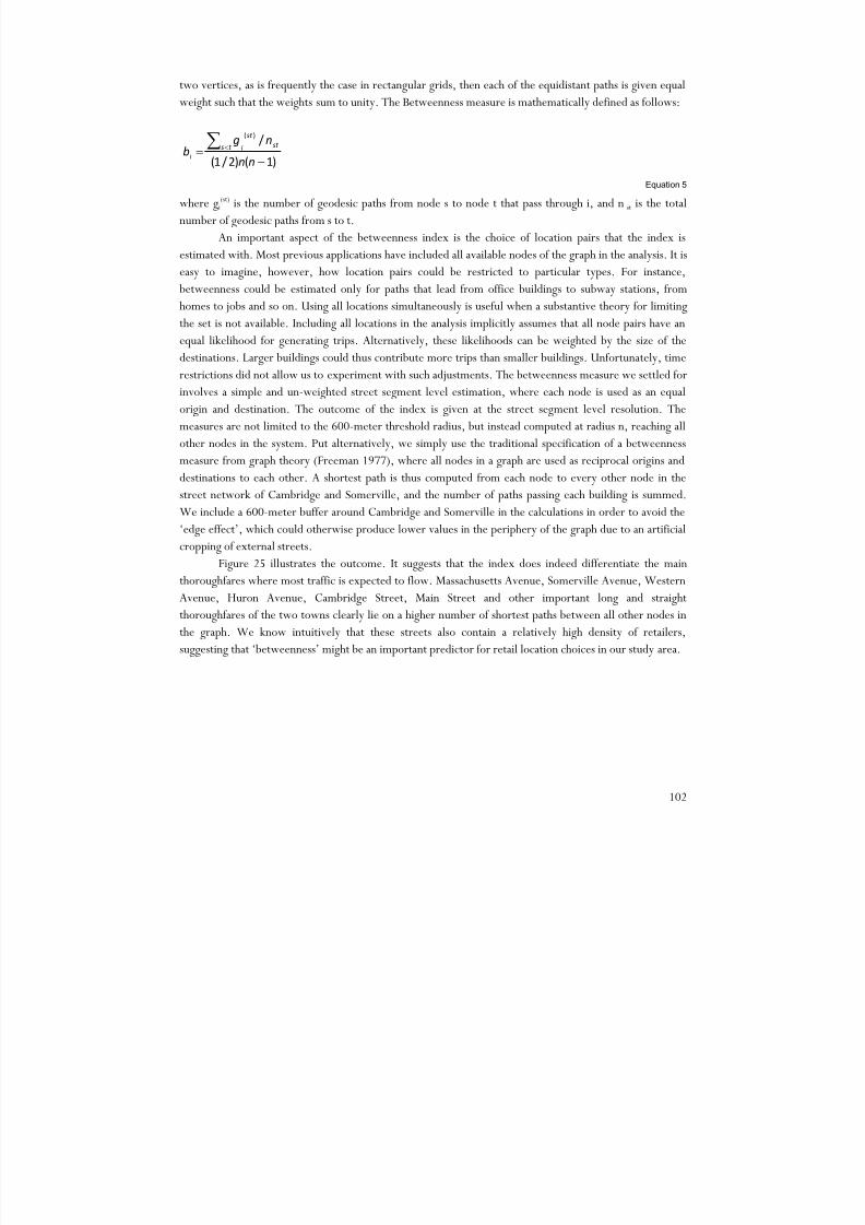
course also related to the human activities that take place therein. Thus, in addressing how environmental
geometry may induce or curb spatial accessibility at different locations within the built environment, we
also need to consider the extents and types of activities that take place in the various buildings that are being
accessed. We argue, however, that it is important to distinguish attributes of accessibility that result from
urban form from those that result from land use attractions. Doing so allows us to investigate whether and
how strongly location choices are affected by each type of variable individually. A clear distinction of factors
allows us to estimate whether retailers cluster in popular locations, such as Central Square in Cambridge,
because of an endogenous attraction to other retailers, to other land uses and transit stations, to
advantageous configuration of urban form, or to a combination of any of these factors.
We center the analysis on one family of economic activities: retail establishments. Retail
establishments offer an interesting case because their attraction to highly accessible locations is well
documented in retail location literature. This allows us to embark on the analysis with a clear set of
hypotheses and expectations. At the same time, we also aim to address important shortcomings in retail
location theory, which is relatively advanced in explaining location patterns in shopping malls, but
remarkably less advanced in explaining retail patterns in urban settings. The bulk of retail location research
of the recent decades has developed using empirical data from privately- and centrally-managed shopping
malls. We do not know whether location patterns encountered in shopping malls are transferable to retail
agglomerations encountered in dense urban environments.
Second, retail location theory has primarily focused on the spatial inter-dependencies betweenretailers. Neo-classical retail location theory, particularly, centers on inter-store externalities, explaining
how the location and characteristics of one store may affect the operations of another store. The state of
knowledge on how exogenous location factors like spatial accessibility and land use attractions may
influence retail location decisions is less good. Focusing exclusively on endogenous location factors and
explaining one store’s location choices with other stores’ location choices overlooks one of the most
interesting questions in economic geography: why do agglomerations form at certain locations in the first
place? Explaining why urban centers in general — and retail agglomeration in particular — emerge at
particular locations in a city remains a glaring shortcoming of economic geography. We suspect that the role
of environmental geometry in this question is central, but poorly understood.
However, the primary purpose of this study is not to improve retail location theory. Instead, the
subject matter explored in this dissertation is foremost driven by the practical necessity to improve our
ability first to comprehend and then to design vibrant and sustainable urban neighborhoods. Nurturing
commercial land uses that support daily retail and service needs at the neighborhood level has become an
important goal in planning environmentally, socially, and economically sustainable urban areas worldwide.
Several recent studies have found that the availability of mixed land uses near one’s place of residence is key
to achieving these goals. A higher concentration of commercial land uses within walking distance reduces
people’s reliance on private automobiles and decreases vehicle miles travelled (Frank and Pivo 1994; Krizek
2003; Zegras 2004), decreases urban energy consumption (Newman and Kenworthy 1999), produces
better health indicators among residents (Hoehner, Ramirez et al. 2005; Rundle, Roux et al. Forthcoming),and fosters social cohesion (Jacobs 1961; Pendola and Gen 2008). From an economic viewpoint, we now
know that clusters of small entrepreneurial businesses produce important agglomeration efficiencies
(Krugman 1991; WorldBank 2009). A diverse set of small establishments tends to generate higher
employment growth and stronger resilience to economic fluctuations and externals shocks than a small set
of large establishments (Glaeser, Kerr et al. 2009). But, despite the abundant evidence on the social,
environmental, and economic efficiencies that commercial establishments within walking range generate,
we are astonishingly incapable of explaining how such land use mixes work, what we can do to sustain
them, and how we could stimulate their development in the countless growing cities around the globe.
Even modest insights into the spatial economic workings of urban retail operations could produce great
value for the contemporary practice of urban design and planning. Analytic methods that are systematic and
replicable in many different urban environments could turn this current shortcoming into a strength. This
dissertation aims to introduce methods of spatial analysis that are easily replicable in the rapidly urbanizing
cities around the World. Taking advantage of recent computational developments, we propose a systematic
approach for detecting location choice preferences that, we hope, will contribute to urban designers’
arsenal of knowledge for creating vibrant and sustainable urban environments.
1.3 Scope of the study
Our research is grounded in two existing bodies of theory: urban economics and configurational
studies of the built environment. Both configurational studies of the built environment and urban economics
have developed important explanations of the spatial distribution of urban land uses. However, mutual
adoption of methods and joint modeling remain lacking between these two fields. Built-form studies have
produced practical methods for measuring socially meaningful properties of the built environment, but their
measures remain largely unused in urban economics. Urban economics, on the other hand, has produced
deep insights into the production functions, linkages and location decisions of households and firms, but
these insights remain underutilized by scholars of city form. This dissertation investigates whether a joint
application of both types of measures could produce a better explanation of the observed pattern of retailers
in a city.
Many attributes of urban form may affect retail location choices. The geometry of an individual
building, for instance, can influence the building’s use — an activity of a certain type and size requires anappropriate spatial shell. A comfortable fit with the layout of the building may well be a decisive criterion
for a particular use. A space that is either too large or small, a disposition of rooms that does not satisfy
desired adjacencies, a circulation system that impedes daily business are but a few instances of spatial misfit
that demonstrate why form needs to follow function.
There is also an aesthetic dimension to urban form. Retailers of a certain type may prefer to locate
in buildings, streets, or neighborhoods that satisfy desired aesthetic standards. Antique dealers, for instance,
might prefer architectural Baroque or Neo-classicism, while art dealers might instead value industrial
structures. Aesthetic qualities of the built environment can sometimes be important factors for location
choices.
Another important quality of urban form for retail location choices is the capacity of the chosen
environment to accommodate growth and change. A business owner who foresees considerable growth
over time might desire a location that can accommodate growth with the least friction possible. Such
retailers might value neighborhoods that are growing or witnessing considerable change. Flexibility towards
future uncertainty can play a decisive role in some stores location decisions.
7
Bardia (for my thesis):there are several issues that we can not approach, due to subjectivity andlack of surveys, such as aesthetic, cognitive, and symbolic aspects of urbanspace.
The analysis presented in this dissertation will, however, not address these attributes of urban
form. A thorough study of ways in which these qualities of urban form affect retail location choices would
require several dissertations. Instead, we will focus on the spatial accessibility of a location: the geometric
layout of building footprints and public spaces and the circulation routes that connect them. The geometric
and topological relationships that emerge from these patterns arrange establishments and people in space by
locating them in relation to each other, at either a greater or lesser degree of agglomeration and separation.
The geometric order of the built environment can thereby engender patterns of movement and encounter
that may incentivize or disincentivize a retail operation. The distribution of land uses, on the other hand,
determines the character of these movements and encounters. The relationship between the configurational
qualities of the built environment and retail location choices seems to provide ample subject matter for a
dissertation, allowing us to develop a more focused investigation than a broader exploration of multiple,
simultaneous, urban form qualities would permit.
The present analysis does not focus on the decision-making process of business-owners who are
about to establish new or move existing stores. Instead, we focus on the ‘revealed’ location choices, where
economic activities have already been located, based on past decisions. We use the observed distribution ofeconomic establishments and a series of attributes of the built environment to infer which factors have
played a significant role in their location choices in the past.
It is important to note that using cross-sectional data in statistical analysis limits our ability to
distinguish causal relationships from mere correlations. We can therefore only speculate whether causality
is present in any of the spatial and social relationships we find. More reliable causal inference could be
developed in future research using longitudinal data and natural experiments.
1.4 Summary of chapters
The next chapter reviews the literature on retail location choices as well as the configurational
studies of the built environment. Discussing both bodies of theory successively, we describe which
problems have been addressed in the past, which aspects of retail location choices remain poorly understood
and outline the areas of overlap that could potentially take both fields in new directions. Chapter Three first
introduces a novel representational framework using graphs, where factors of urban form, land use, and
travel behavior can be jointly depicted. This framework allows us to represent the problem of location
choices, and to measure detailed attributes of spatial accessibility in our study area. We then introduce our
case study area of Cambridge and Somerville MA, and describe the various predictors of retail location
choices that were captured for the analysis that follows. The second half of the chapter introduces the
empirical estimation methodology. An innovative spatial econometric model is proposed, where three types
of important effects on retail location choices can be jointly estimated. First, the methodology includes a
strategic interaction component that allows us to evaluate the degree to which location choices depend
endogenously on other establishments’ presence in the neighborhood. Second, the methodology includes a
set of exogenous variables that predict how the spatial and economic characteristics around each location
may affect retail location choices. And third, the methodology addresses the hazard of omitted variables that
are often found in spatial location choice studies. Having introduced the methodology, Chapter Four will
A field of configurational studies of the built environment developed among architects, planners, and
transportation researchers in the 1960s and 70s. The work is characterized by attempts to understand the
societal forces that shape settlement patterns and to develop analytic methods that outline meaningful
properties of environmental geometry (See March and Steadman 1971; Martin and March 1972; Anderson
1978; Hillier and Hanson 1984; Habraken and Teicher 1998; Porta, Crucitti et al. 2005). This work has
also investigated effects that environmental geometry might have on the performance and quality of cities
(Weeks 1960; Proshansky, Ittelson et al. 1970; Tabor 1976; Lynch 1984; Ellingham and Fawcett 2006) by
analyzing the relationship between social behavior and spatial configuration using both quantitative and
qualitative methods, which range from mathematical geometry and graph theory to ethnographic surveys
and comparative analysis. Scholars of this field have a deep understanding of environmental geometry and
are primarily interested in understanding or measuring the social significance of architectural and urban
form.
Around the same time, land use location theory, a different field, but equally concerned with urban
space, emerged in economics. The scholars of location theory focus on the spatial distribution of land uses,
firm location choices, and land values (Lösch 1954; Isard 1956; Alonso 1964; Mills 1967; DiPasquale and
Wheaton 1996). They seek to understand how various individuals and groups with different interests and
requirements compete for locations and produce the observed urban land use pattern. Whereasconfigurational studies are predominantly concerned with the geometry of the environment, urban
economics centers on the efficiencies that result from a spatial interaction between land uses. Configuration
of the environment is of interest to urban economics insofar as it constitutes the spatial stage where market
competition occurs, imposing transportation and time costs for interaction. Details of spatial configuration
have typically been of minor interest in the these studies: “The city is viewed as if it were located on a featureless
plain, on which all land is of equal quality, ready for use without further improvements, and freely bought and sold ”
(Alonso 1964). Newer land use and accessibility models often operate implicitly within the actual geometry
of the street network, representing spatial relationship between locations by a time or distance cost along
shortest-travel paths (Wyatt 1997; Bhat, Handy et al. 2002; Waddell and Ulfarsson 2003). However, the
interaction between the distribution of land uses and the configuration of city form has not been an explicit
area of research in urban economics. Understanding this interaction is important for planners. How are firm
location decisions affected by advantages in accessibility set by environmental geometry? How is the spatial
configuration of the city in turn affected by the requirements posed by urban land uses? What land use
attractions and configurational characteristics of locations make them more or less suitable for certain types
of uses? The relationship between urban economics and urban design is generally under-examined and little
understood, making desirable even modest advances in unbundling the social and economic significance of
city form.
This dissertation aims to overlap a detailed configurational study of urban form with an economic
analysis of location choices. Both configurational studies of the built environment and urban economics have
developed important explanations about the spatial distribution of land uses. But a mutual adoption of
methods and joint modeling remains lacking. Built-form studies have resulted in practical methods formeasuring socially meaningful properties of the built environment (March and Steadman 1971; Martin and
March 1972; Anderson 1978; Steadman 1983; Hillier and Hanson 1984), but their measures remain largely
unused in urban economics. Urban economics, on the other hand, has evaluated location choices with
respect to production functions and economic linkages to suppliers or customers, largely ignoring
environmental geometry (Huff 1963; Waddell and Ulfarsson 2003; Huang and Levinson 2008). Earlier
writings of Proudfoot and Hurd have explicitly commented on the configurational aspects of location at
neighborhood scale (Hurd 1903; Proudfoot 1937), and configurational questions are implicit in some
scholars’ research on location choices (Carter and Vandell 2005), but an explicit focus on the effects of
environmental geometry on location values has not been central in either field. Empirical research
presented in this dissertation moves towards a joint approach, where spatial attributes of the built
environment are evaluated from an economic perspective of land use location choices. We conjecture that a
joint usage of both types of measures could produce a better explanation of the observed urban structure,
and we hypothesize that environmental geometry could be an important determinant of economic location
choices.
2.1 Classical retail location theory
The spatial distribution of retailers has been widely studied by scholars of the city. Already in 1916Robert Park noted that “There is now a class of experts, whose sole occupation is to discover and locate, with something
like scientific accuracy, taking account of the changes which present tendencies seem likely to bring about, restaurants,
cigar stores, drug-stores, and other small retail business units whose success depends largely on location. Real estate men
are not infrequently willing to finance a local business of this sort in locations which they believe will not be profitable,
accepting as their rent a percentage of the profits” (Park 1916: 95). Proudfoot categorized the principle spatial
patterns of retailers of early 20th-century American cities into five groups according to commodities sold,
12
blemtementource:
igurationa
dies of the
ronment
urban
omics
loped
ortant
anations
t theal
ibution of
uses. But
tual
tion of
hods and
modeling
ains
ng
Newer land use and accessibility models often operate implicitly within the actual geometry of the street
network, representing spatial relationship between locations by a time or distance cost along shortest-travel
paths (Wyatt 1997; Bhat, Handy et al. 2002; Waddell and Ulfarsson 2003)
concentration or dispersal of outlets, and customer type: (1) the central business district; (2) the outlying
business center; (3) the principal business thoroughfare; (4) the neighborhood business street; and (5) the
isolated store cluster (Proudfoot 1937). These five patterns of retailing continue to this day, with a few
additions. Over the course of the 20th-century the car-oriented shopping mall, which is somewhat analogous
to Proudfoot’s outlying business center, has become one of the most important retail typologies of our
time. Much of retail location literature has come to focus on this typology. An isolated general store, big
enough to supply all quotidian merchandise, the strip-mall, which resembles Proudfoot’s principal business
thoroughfare, but serves a predominantly vehicular clientele, and the non-store retailer (i.e. catalogue,
phone or internet order) might also be added to the list of prominent 20th-century retail typologies.
Several economic forces that shape the densities and location patterns of retailers have found an
explaination since Park’s and Proudfoot’s writing. Previous comprehensive reviews of retail store location
theories have been given by Isard, Berry, Stahl, Vandell and carter, and Eppli and Benjamin among others
(Isard 1956; Berry 1967; Stahl 1987; Vandell and Carter 1993; Eppli and Benjamin 1994). A review of
different mathematical models for predicting potential store locations are given by Huff, O’Kelley,
Achabal, Gorr, and others (Huff 1963; O'Kelly 1981; Achabal, Gorr et al. 1982; Ghosh, Craig et al. 1984).Popular sources of recent publications include: The Journal of Retailing, The Journal of Real Estate
Research, and Journal of Real Estate Literature.
A typical retail location model postulates that store owners are expected to locate at points of
maximal demand, “as closely as possible to the consumers demanding their commodity bundle; and to
retailers who, by supplying complementary commodity bundles, attract the desired clientele” (Stahl 1987:
759). Location decisions also need to account for direct competitors, by balancing the potential of higher
demand that results from clustering with competitors against the monopolistic advantages of increased
market area that result from locating in isolation. The choice of location thus directly affects the patronage
and revenues of retail establishments and constitutes an important part of a retailer’s production function1.
2.1.1 A one-dimensional model
DiPasquale and Wheaton illustrate a simple classical model, where store location choices happen on
a one-dimensional straight line (DiPasquale and Wheaton 1996). The model starts with the point of view of
consumers, whose shopping frequencies collectively constitute the aggregate demand for retailers.
Consumers’ decisions of shopping frequency are viewed as a cost-minimization problem. Total costs in this
scenario signify the combined costs of purchase prices and transportation costs, as well as inventory costs tostore merchandise at home. Shopping frequency thus depends on the type of commodity bought, the
frequency of its use, and the transportation costs of delivering it. The total annual cost (C) of consuming a
good is given by the annual purchase price of the units Pu (unit price P times the amount purchased annually
u), the annual transportation costs for delivering the good kv (transportation costs per trip k times trip
1 Retailers also compete for customers through prices and choice of merchandise.
frequency v ), and the inventory costs: storage cost per year i times the purchase value of the average
inventory between two shopping trips Pu/2v (DiPasquale and Wheaton 1996: 132):
⎟ ⎠
⎞⎜⎝
⎛ ++=
v
Puikv PuC
2
Equation 1
Consumers are thought to adjust their shopping frequency so as to minimize their total costs C . This
minimization problem is solved by equating the first-order derivative of Equation 1with respect to v to
zero, which leads to an optimal purchase frequency v*:
2
1
2* ⎟
⎠
⎞⎜⎝
⎛ =
k
iPuv
Equation 2
The inspection of the optimal purchase frequency (v*) in Equation 2 is telling with regard to
consumer shopping behavior. If transportation costs (k) are higher, then all else equal, shopping frequency(v*) is lower. If storage costs (i) are higher, as is the case with perishable goods for instance, then shopping
frequency is higher. Similarly, if the amount consumed annually rises, then all else equal, purchase
frequency rises. Items that rarely amortize or perish and those that are hard to store (e.g. furniture items)
are purchased at a lower frequency. Retailers selling infrequently-purchased goods are thus expected to
locate at larger intervals and to draw customers from larger market areas than neighborhood grocery stores.
However, the exact spacing of different types of retailers also depends on the fixed costs of establishing and
running a business and the pricing policy of competitive retailers. Lower prices can compensate customers
for longer trips.
A given purchase frequency leads to a model that explains store-owners location decisions. This
model estimates the expected density of retail facilities as a function of four parameters:
v: frequency of purchase trips
k: costs of travel per mile
C: fixed cost for a retail facility
F: buyer density in a given linear radius
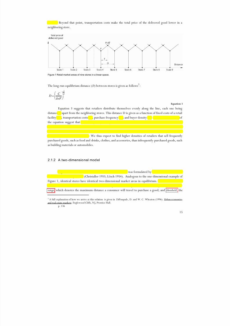
Customers are assumed to be uniformly distributed along a horizontal line, as shown in Figure 3.
The model assumes that all retailers offer identical products. Consumers are expected to shop at the retailer
whose total delivered price for the good is lowest. The total delivered price of an item is the sum of the
purchase price P and the travel cost kD (travel cost per mile times distance). In equilibrium, each store hasidentical sales prices2 and an equal-size double-sided market area (2T ), inside of which it offers the lowest
delivered price for consumers located within that zone (DiPasquale and Wheaton 1996: 136). The market
area between two stores is defined as the point where the total delivered cost is equal between two stores
2 Reaching identical prices in equilibrium is just one theory according to Tirole, J. (1988). Theory of Industrial Organization.Cambridge, MIT Press.
14
Bardia: Pu/2v because: pu is the yearly purchasing, so each time the purchase will be pu/v (v frequ
of travel). assuming the consumption between two trips as a unique function, then the average storag
pu/2v (because it is equal to pu/v just after a trip and 0 just before a trip)
(P+kT ). Beyond that point, transportation costs make the total price of the delivered good lower in a
neighboring store.
Figure 1 Retail market areas of nine stores in a linear space.
The long-run equilibrium distance (D) between stores is given as follows3:
D = C
kvF
⎛
⎝⎜
⎞
⎠⎟
1
2
Equation 3
Equation 3 suggests that retailers distribute themselves evenly along the line, each one being
distance D apart from the neighboring stores. This distance D is given as a function of fixed costs of a retail
facility (C), transportation costs (k), purchase frequency (v), and buyer density (F). Descriptive statistics of
the equation suggest that if the frequency of trips (v) increases, then the distance between facilities (D)
decreases and the density of facilities is higher. If the fixed costs of setting up a facility (C) rise, then the
distance between facilities also rises, and density decreases. As the density of customers (F) goes up, thedensity of facilities also goes up. We thus expect to find higher densities of retailers that sell frequently
purchased goods, such as food and drinks, clothes, and accessories, than infrequently-purchased goods, such
as building materials or automobiles.
2.1.2 A two-dimensional model
A general two-dimensional model of retail distribution was formulated by Christaller and Lösch in
Central Place Theory (CPT) (Christaller 1933; Lösch 1954). Analogous to the one-dimensional example ofFigure 1, identical stores have identical two-dimensional market areas in equilibrium. The size of market
areas and the distance between stores are ultimately determined by two fundamental inputs to the model:
range, which denotes the maximum distance a consumer will travel to purchase a good; and threshold , the
3 A full explanation of how we arrive at this solution is given in DiPasquale, D. and W. C. Wheaton (1996). Urban economicsand real estate markets. Englewood Cliffs, NJ, Prentice Hall.
minimum demand necessary for a store to stay in business. Christaller and Lösch illustrate how the
combination of range and threshold leads to a regular hexagonal pattern of stores, where the size of the
hexagons is determined by the maximum range of customers and the minimum threshold of the store.
Identical stores divide the market areas evenly, with each store being equidistant from neighboring stores
selling the same goods, as shown in Figure 2.
Figure 2 Market areas of identical stores in Central Place Theory .
Similar stores have similar market areas, but stores offering different goods can have different
market areas. As bread, for instance, is bought frequently, a relatively small market area will generate
enough demand for a bread store to remain viable. Furniture, on the other hand, is bought rarely, and so
market areas of furniture stores must be correspondingly large. Smaller retailers, which attract more
frequent purchase patterns, can thus emerge at the boundaries of larger retail market areas. For a single
region, there might be several bread stores and only one (or no) furniture stores. These differences lead to
overlapping market areas, where hexagons of higher-order goods, which are rarely bought or otherwise
require large market areas to remain viable, reach across market areas of lower-order goods, as illustratedin Figure 3. Higher-order centers combine a wider variety of different stores, while lower-order centers
only offer goods that can be supported by a smaller market area.
Figure 3 Overlapping market areas of hierarchical centers in Central Place Theory
The hexagonal pattern of centers in Figure 3 describes the most economic pattern of development that can
serve an even distribution of customers with a minimum number of centers. But it is important to note that
the emergence of hexagonal market areas assumes a spatial environment that resembles a featureless plain,
on which all land is of equal quality, ready for use without further improvements. Consumers are assumed
to obtain a particular good only from the nearest center and to make a separate trip for each type of
merchandise. Customers are assumed to approach centers along straight-line travel paths from any point in
the region.
The absence of a spatial transportation network in CPT leads to a spatial puzzle. If one were to
commute between higher- and lower-order centers in the hexagonal pattern of Figure 3, a fundamental
transportation inefficiency would appear: routes connecting two higher order centers, passing through
lower order centers, would be crooked, not straight, as transportation economies would suggest.
Christaller acknowledged the issue by evoking Kohl’s traffic principle (Kohl 1850), according to which travel
routes are expected to follow most economical paths between centers:
“One sees immediately that if the central places are distributed according to the traffic principle, a considerably higher
number of central places of each type will be necessary in order to supply the region with central goods of a particular
range. This contrasts with the marketing principle, which economizes on the number of central places required to supply
the whole land. Both principles are theoretically correct, as both are, in a certain sense of the word, of the highest
rationality. But there can be only one possibility with the highest economic rationality. Which possibility it is will
depend upon the concrete circumstances. Either the traffic principle has such a weight that it outweighs the marketing
principle, advantage for advantage, or the marketing principle is the stronger one, or finally, the most favorable system is
obtained through a combination of both principles, i.e., through a compromise”. (Christaller and Baskin 1966: 74)
However, he later concluded that “Since the marketing principle is clearly dominant in determining the
distribution of the central places in Southern Germany, we may say, generally then, that the marketing principle is the
primary and chief law of distribution of the central places. The traffic and the separation principles are only secondarylaws causing deviations; these laws are effective in practice only under certain conditions.” (Christaller and Baskin
1966: 192)
The marketing principle of CPT, which suggests the most economical hexagonal pattern of centers,
and Kohl’s traffic principle, which emphasizes the economies of travel routes, thus produces a theoretical
dichotomy: is the spatial evolution of the pattern driven by an efficient allocation of centers or by efficient
commuting between centers? The resolution is not essential to CPT, since inter-center commuting in
general and multipurpose shopping in particular are not addressed in the theory. Similar to the one-
dimensional market area analysis of the preceding section, CPT assumes that consumers make a separate
trip for each good and always shop at the nearest center. Goods offered in different centers are thus
assumed to be acquired on different trips, and inter-center transportation inefficiencies therefore do not
affect the model.
CPT has propagated a great deal of empirical research. Christaller produced the first assessment of
Central Places in Southern Germany in his original publication (Christaller 1933). Similar findings were
contemporaneously produced in Estonia by Edgar Kant (Kant 1933; Kant 1935). Evidence of Central Places
in the United States is given by Berry, who used data from rural Iowa and urban Chicago (Berry 1967).
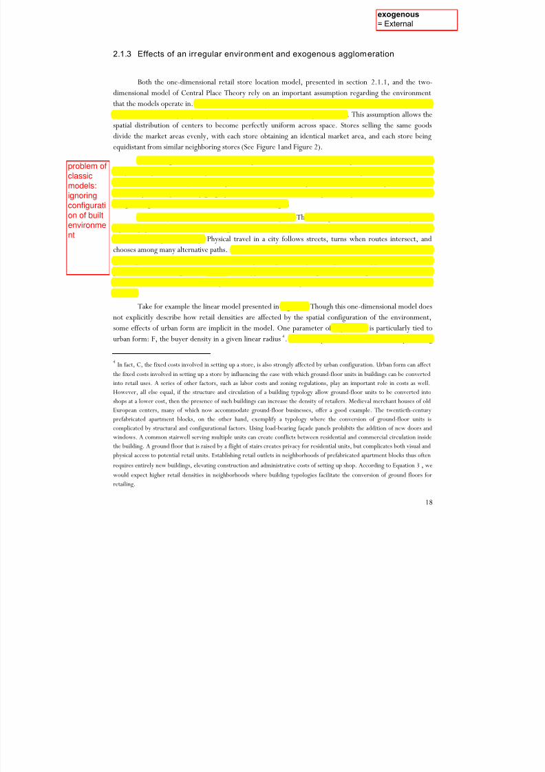
2.1.3 Effects of an irregular environment and exogenous agglomeration
Both the one-dimensional retail store location model, presented in section 2.1.1, and the two-
dimensional model of Central Place Theory rely on an important assumption regarding the environment
that the models operate in. Both models assume a spatial environment that resembles a featureless plain, onwhich all land is of equal quality, ready for use without further improvements. This assumption allows the
spatial distribution of centers to become perfectly uniform across space. Stores selling the same goods
divide the market areas evenly, with each store obtaining an identical market area, and each store being
equidistant from similar neighboring stores (See Figure 1and Figure 2).
The homogenous environment assumption is, of course, a coarse simplification that clarifies the
analysis and produces a more parsimonious model. It eliminates the role of transportation networks and
urban form from the analysis, allowing location patterns to emerge in response to marketing forces that can
flow freely across space in any geographic direction. A consumer is expected to patronize the closest center
using a straight-line route from his or her location of origin.
The reality of built environments is more complex. The homogenous environment assumption is
especially problematic when analyzing land use location patterns within a city — which is the central
concern of the present study. Physical travel in a city follows streets, turns when routes intersect, and
chooses among many alternative paths. The geometric configuration of the urban street network and transit
system generates an uneven level of accessibility throughout a city, limiting access to opportunities in some
places, while favoring it in others. We hypothesize that the geometric configuration of the built
environment can thus exert an important influence on the spatial distribution of centers in intra-urban
settings.
Take for example the linear model presented in Figure 1. Though this one-dimensional model does
not explicitly describe how retail densities are affected by the spatial configuration of the environment,
some effects of urban form are implicit in the model. One parameter of Equation 3 is particularly tied to
urban form: F, the buyer density in a given linear radius 4. The density of customers is affected by building
4 In fact, C, the fixed costs involved in setting up a store, is also strongly affected by urban configuration. Urban form can affect
the fixed costs involved in setting up a store by influencing the ease with which ground-floor units in buildings can be converted
into retail uses. A series of other factors, such as labor costs and zoning regulations, play an important role in costs as well.
However, all else equal, if the structure and circulation of a building typology allow ground-floor units to be converted into
shops at a lower cost, then the presence of such buildings can increase the density of retailers. Medieval merchant houses of old
European centers, many of which now accommodate ground-floor businesses, offer a good example. The twentieth-century
prefabricated apartment blocks, on the other hand, exemplify a typology where the conversion of ground-floor units iscomplicated by structural and configurational factors. Using load-bearing façade panels prohibits the addition of new doors and
windows. A common stairwell serving multiple units can create conflicts between residential and commercial circulation inside
the building. A ground floor that is raised by a flight of stairs creates privacy for residential units, but complicates both visual and
physical access to potential retail units. Establishing retail outlets in neighborhoods of prefabricated apartment blocks thus often
requires entirely new buildings, elevating construction and administrative costs of setting up shop. According to Equation 3 , we
would expect higher retail densities in neighborhoods where building typologies facilitate the conversion of ground floors for
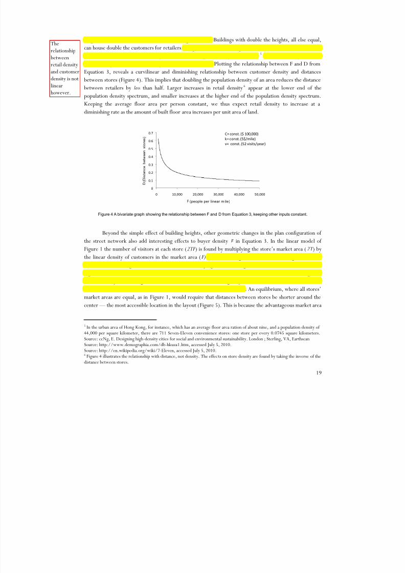
heights and the floor area ratio (FAR) of a neighborhood. Buildings with double the heights, all else equal,
can house double the customers for retailers. Neighborhoods where higher residential densities are achieved
with taller structures are thus expected to have a higher density of retailers. 5 The relationship between
retail density and customer density is not linear however. Plotting the relationship between F and D from
Equation 3, reveals a curvilinear and diminishing relationship between customer density and distances
between stores (Figure 4). This implies that doubling the population density of an area reduces the distance
between retailers by less than half. Larger increases in retail density 6 appear at the lower end of the
population density spectrum, and smaller increases at the higher end of the population density spectrum.
Keeping the average floor area per person constant, we thus expect retail density to increase at a
diminishing rate as the amount of built floor area increases per unit area of land.
0
0.1
0.2
0.3
0.4
0.5
0.6
0.7
0 10,000 20,000 30,000 40,000 50,000
D
( D i s t a n c e
b e t w e
e n
s t o r e s )
F (people per linear m ile)
C=
const.
($
100,000)
k= const.
(5$/mile)
v= const. (52 visits/year)
Figure 4 A bivariate graph showing the relationship between F and D from Equation 3, keeping other inputs constant.
Beyond the simple effect of building heights, other geometric changes in the plan configuration ofthe street network also add interesting effects to buyer density F in Equation 3. In the linear model of
Figure 1 the number of visitors at each store (2TF ) is found by multiplying the store’s market area (2T ) by
the linear density of customers in the market area (F). If we rearrange the nine stores of Figure 1 into a
different linear configuration, a cross for instance, keeping the linear length of streets constant, as shown in
Figure 5, then different locations within the network face different access to customers. Assuming that
travel can only occur along the linear lines that form the cross (e.g. city streets), a store at the center would
have four times the access reach of stores at the far ends of the cross arms. An equilibrium, where all stores’
market areas are equal, as in Figure 1, would require that distances between stores be shorter around the
center — the most accessible location in the layout (Figure 5). This is because the advantageous market area
5 In the urban area of Hong Kong, for instance, which has an average floor area ration of about nine, and a population density of44,000 per square kilometer, there are 711 Seven-Eleven convenience stores: one store per every 0.0745 square kilometers.Source: ccNg, E. Designing high-density cities for social and environmental sustainability. London ; Sterling, VA, EarthscanSource: http://www.demographia.com/db-hkuza1.htm, accessed July 5, 2010.Source: http://en.wikipedia.org/wiki/7-Eleven, accessed July 5, 2010.6 Figure 4 illustrates the relationship with distance, not density. The effects on store density are found by taking the inverse of thedistance between stores.
at the center would, in the long run, be reduced by stores moving closer to the center until all store’s
market areas are equal. Keeping the total number of stores constant, this would lead to a higher density of
stores around the center of the cross than in the outlying areas. The geometry of the environment thus
generates shorter distances between stores at more accessible locations.
Figure 5 Equal-size retail market areas of nine stores on a cruciform linear network.
Environmental geometry can further augment store density as localized levels of accessibility
increase. Unusually high levels of accessibility, which could result from an atypical intersection of numerous
streets or the presence of a subway stop, could lead to the emergence of clusters of competitive stores.
Additional retailers would be expected to join the cluster until profits resulting from advantageous
accessibility are dampened though competition. The cluster would stop growing when enough retailers
have entered a cluster to lower profits to the same level as the next best alternative location. The scenario
thus illustrates an exogenous agglomeration process, whereby retailers do not agglomerate because of
mutual complementarily or because of proximity to suppliers, but rather because the spatial configuration
of the environment supplies certain locations with better access to customers.
Analogous effects of environmental geometry on retail location choices are typically missing from
economic location studies. This might be partially explained by the complexity that spatial irregularities
introduce to the models, and/or the lack of established conventions for measuring spatial configuration.
The analysis of location patterns on networks has, however, recently become graspable with the aid of
computers. GIS Network Analyst7, TransCAD8, SANET9, GeoDaNet10, NetworkX11, and UCL
DepthMap12
currently offer some of the most popular software platforms for spatial network analysis,making the laborious task of computing location attributes on a network manageable. Meanwhile, research
7 http://www.esri.com/software/arcgis/extensions/networkanalyst/index.html (Accessed February 17, 2010)8 http://www.caliper.com/tcovu.htm (Accessed February 17, 2010)9 http://sanet.csis.u-tokyo.ac.jp/ (Accessed February 17, 2010)10 http://geodacenter.asu.edu/software (Accessed February 17, 2010)11 http://networkx.lanl.gov/ (Accessed February 17, 2010)12 http://www.vr.ucl.ac.uk/depthmap/ (Accessed February 17, 2010)
on configurational studies of city form has made significant theoretical progress in proposing appropriate
measures to describe variations in accessibility that result from urban form. We shall review some of these
techniques in greater detail later in this chapter.
2.2 Neo-classical Retail Location Theory and Endogenous Agglomeration
The last section presented an example of exogenous clustering, where the density of competitive stores
increased in the part of a network where spatial access was geometrically favorable. We call such clustering
exogenous since it is attributable to an external resource, which all retailers are attracted to. However,
retail agglomeration can also arise from endogenous factors: externalities between retailers that make it
inherently beneficial for stores to locate in close proximity to each other. These externalities form the
central focus of neo-classical retail location theory.
2.2.1 Transpor tation Savings and the Clustering of Complementary Stores
Empirical studies of retail distribution over the 20th-century have increasingly accumulated evidence that
challenges the predictions of Central Place Theory. The single-purpose, nearest-center patronage
assumption of CPT has attracted most criticism. Multiple empirical studies have shown that people do not
always choose the closest shopping venues and that they often shop at multiple stores on the same trip.
Using data similar to Berry’s, Rushton, Golledge, and their colleagues showed that only 35% of a rural
Iowa population shopped at the nearest center (Rushton, Golledge et al. 1967). Clarke, using data from
New Zealand, showed that the nearest-center patronage assumption becomes less tenable as the size of the
destination center increases (Clark 1968). Whereas 63-83% of trips to small shopping centers patronized
the nearest destinations, only half of the trips led to the closest destination among largest centers. The
difference is explained, the authors argue, by transportation savings achieved by multipurpose shopping at
the larger centers. Hanson studied explicitly whether shopping trips are multipurpose and found that 61%
of all trips in his sample were multipurpose (Hanson 1980). Similarly, O’Kelly found that 63% of grocery
shopping trips and 74% of non-grocery trips were multipurpose (O'Kelly 1981).
Multipurpose shopping introduces inter-store externalities to a retail location model, challenging the
store distribution predictions of CPT. Transportation savings that arise in multipurpose shopping bias
consumers in favor of larger centers. If a similar bundle of goods can be acquired by either patronizingdisparate small stores on multiple trips or a large and heterogeneous cluster on a single trip, then the latter
option often leads to a lower total cost due to savings in transportation.13 As a larger variety of goods draw
a larger pool of customers, a positive feedback loop incentivizes stores to cluster in even larger
13 This is of course ignoring other potentially important factors of destination choice, such as emotional pleasure, which couldlead to the patronage of multiple isolated small stores despite the additional transportation cost.
heterogeneous centers (Bacon 1971; Mullingan 1987). Eaton and Lipsey have shown how multipurpose
shopping on the part of consumers and profit maximizing locational choice on the part of firms can lead to a
higher concentration of clusters than predicted in CPT (Eaton and Lipsey 1982). West, Hohenbalken, and
others have corroborated this effect using empirical evidence from Edmonton, Alberta:
“Our tests support the hypothesis of a hierarchy of shopping centres with properties that are more closely aligned to an
Eaton and Lipsey than a Christaller-type hierarchy. In particular, we found that our shopping centre hierarchy has one
important characteristic that is consistent with the predictions of the Eaton and Lipsey model, but not Christaller's,
namely the replication of stores of the same type in the same shopping centre. We would expect such replications to arise
naturally from the profit maximising locational behaviour of firms confronted with comparison and multipurpose
shopping behaviour on the part of consumers (behaviour that is outside the Christaller model, but within those developed
by Eaton and Lipsey)”. (West, Hohenbalken et al. 1985: 116).
Though multipurpose shopping has mainly been used to explain the success of shopping malls, its
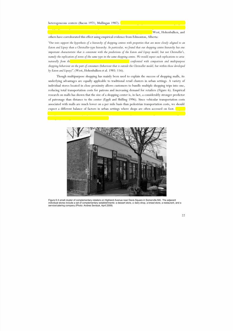
underlying advantages are equally applicable to traditional retail clusters in urban settings. A variety of
individual stores located in close proximity allows customers to bundle multiple shopping trips into one,
reducing total transportation costs for patrons and increasing demand for retailers (Figure 6). Empiricalresearch on malls has shown that the size of a shopping center is, in fact, a considerably stronger predictor
of patronage than distance to the center (Eppli and Shilling 1996). Since vehicular transportation costs
associated with malls are much lower on a per mile basis than pedestrian transportation costs, we should
expect a different balance of factors in urban settings where shops are often accessed on foot. Higher
transportation costs make people more sensitive to distances required to reach larger centers, leading to a
stronger patronage of closer and smaller stores.
Figure 6 A small cluster of complementary retailers on Highland Avenue near Davis Square in Somerville MA. The adjacentindividual stores include a set of complementary establishments: a dessert store, a dairy shop, a bread store, a restaurant, and aservice/catering company (Photo: Andres Sevtsuk, April 2009).
Neo-classical retail location theory suggests that multipurpose shopping also introduces a
second, related effect to explain the clustering of heterogeneous and complementary stores: demand
externalities. Demand externalities refer to customer spillovers that one store can produce for other stores.
Given conveniently small distances between stores, customer traffic attracted to higher-order retailers can
increase traffic in lower-order retailers. Unlike the transportation effect in multi-purpose shopping, where
heterogeneous clusters enable customers to purchase a set of planned goods at lower total costs, demand
externalities produce additional unplanned purchases in lower-order stores. A customer visiting a
department store in a mall, for instance, might pay a visit to a newspaper kiosk in the same mall, thus
making a purchase that he or she would avoid if a separate trip to a newspaper kiosk were required.
Demand externalities are generally thought to flow in one direction — from more popular to less popular
stores or from anchor stores to non-anchor stores.
Brueckner has provided a model that demonstrates how a careful manipulation of the size of stores in
a shopping center, according to their level of demand externalities and their impact on the center as a
whole, can maximize shopping center revenues (Brueckner 1993). In his model, the sales volume of a store
i, denoted as Ri, depends on the amount of space Si that the store occupies14
. In the presence of inter-storeexternalities, Ri also depends on the amount of space allocated to other stores in the center. Store i’s sales
are thus given as a function of all stores’ areas in the center:
Ri = Ri (S1, S2, …, Sn ), where
∂∂
0 ∂∂
0,
Equation 4
Equation 4 shows that as store i’s own space rises, then sales at store i are also expected to rise.
However, if a nearby store j produces positive demand externalities for store i, then store i’s sales can also
rise as store j’s floor area increases. If no externalities exist between i and j, then the marginal effect of
store j’s space increase on store i’s sales can also be zero. However, if a center contains multiple stores of a
given type, then competition between stores might reverse this effect. For instance, if store i and j are both
shoe stores, then ∂Ri/∂S j and ∂R j/∂Si could both be negative as an increase in the size of store i reduces the
sales of the competing store j and vice versa. Brueckner goes on to show how a careful and coordinated
manipulation of complementary store sizes can lead mall-owners to optimal profits for the center as a
whole.
A large body of empirical research has studied demand externalities in shopping malls. Anikeeff
provides an overview of previous attempts to measure the degree of spillovers, or ‘‘retail compatibility,’’across different types of non-anchor stores (Anikeeff 1996). Nelson classified stores into five categories
according to the percentage of customers who visit a given pair of stores (Nelson 1958). More recently,
Eppli and Shilling used a new dataset and enhanced methods to re-estimate the degree of retail compatibility
for a sample of stores in fifty-four regional shopping centers in the United States (Eppli and Shilling 1993).
14 Space is used as a proxy variable for capturing the choice of merchandise at the sore.
23
mandernality
Bardia: dRi/dSj>=0; it means that negative
spillover is not considered. Typically shops would
They found that regional shopping centers with greater quantities of space devoted to anchor tenants have
higher non-anchor tenant sales for eight out of nine merchandise types.
Theories on profitable mixing of tenants in planned shopping malls have also led numerous
researchers to look for implicit evidence of demand externalities embodied in tenants’ rent contracts. In a
widely popular practice, mall owners charge a discriminatory percentage of rent from tenants, depending
on their impact on not only their own revenues, but also on the revenues of the mall as a whole 15. Stores
that constitute the primary motivation for customers’ trips to the center (i.e. department stores), generally
pay low or no rent, while odd specialty stores that are not on the list of many shoppers pay high rents, as
most of their traffic comes from nearby stores. This difference in rents is seen as implicit evidence of
demand externalities that anchor stores generate for non-anchor stores. Empirical evidence of differential
rents is given by (Benjamin, Boyle et al. 1990; Benjamin, Boyle et al. 1992).
Centrally-managed private shopping centers offer cheaper percentage rent contracts as an incentive
to attract big anchor stores to the center. The positive demand externalities that such stores create for other
stores are thereby returned in the form of cheaper rent payments. Eppli and Benjamin have shown that the
image and fame of anchor stores (i.e. brands) play an important part in customer draw, often increasing thecustomers willingness to patronize otherwise distant locations (Figure 7) (Eppli and Benjamin 1994).
Figure 7 Porter Square Mall in Porter Square, Cambridge MA. A careful manipulation of demand externalities and rent contracts
allows mall owner to maximize profits by orchestrating an optimal tenant mix. The part of the mall on the image contains only well-known brand stores: a Dunkin’ Donuts coffee shop, a Mexican Grill restaurant, a RadioShack electronics store, a Liquor World alcohol store, and a Zoots drycleaner.(Photo: Andres Sevtsuk, April 2009)
15 There is a debate over the question of whether these discriminatory rents favor mall owners or mall tenants. See Wheaton, W.C. (2000). "Percentage Rent in Retail Leasing: The Alignment of Landlord--Tenant Interests." Real Estate Economics 28(2):185-204.
It is generally agreed in retail location literature that a profitable orchestration of complementary
stores in planned shopping malls, coupled with discriminatory rent contracts that attract anchor stores to
the center, is the primary reason why shopping malls have managed to eclipse other traditional forms of
retailing in the US in the course of the 20th-century. Unlike main streets and neighborhood retailers,
private shopping malls purposefully coordinate the tenant mix, prohibiting ‘unwanted’ store entry to the
center and optimizing the performance of the cluster as a whole. A central management system allows
owners to choose only stores that increase mall revenues by either attracting additional customers or paying
higher rents for positive demand externalities, so that the positive externalities produced by higher-order
stores are perfectly balanced by lower rents per square foot, thus providing all stores an equal incentive to
join the center. Without subsidized rent contracts, anchor stores would face a disincentive to locate in
shopping malls, since their customer draw would generate positive externalities for other stores with no
compensation for the favor. Such is the case, however, in uncoordinated urban retail clusters (i.e. main
streets, neighborhood centers, etc)16. This suggests that we should not expect the store clusters and
agglomeration patterns found in shopping malls to appear analogous in urban settings. Instead, we expect
clustering preferences to vary among different types and sizes of retailers. Non-anchor stores, such as smallretailers who offer a limited choice of infrequently purchased merchandise, are more likely to value
heterogeneous cluster locations, because the availability of complementary stores in a cluster enables
customers to acquire a larger assortment of products from a single location, saving transportation costs and
offering an incentive to visit the cluster. Large anchor stores, on the other hand, do not benefit from urban
cluster locations in the same way that they do in malls. By attracting a large customer pool, they generate
positive externalities for lower-order stores, without receiving rent subsidies or other types of return for
the deed. We suspect that this might lead some anchor-stores to avoid cluster locations.
Retail location literature has been relatively silent on un-coordinated retail clusters17. The literature
on demand externalities is especially vague about externalities in urban settings. Anecdotal evidence
suggests that large anchor stores, such as supermarkets, are found equally often in free-standing locations as
in neighborhood retail clusters. It is unclear if choosing a free-standing location is a result of an endogenous
repellent force that drives large stores away from clusters or simply an exogenous attraction towards
different types of locations, such as locations that are closer to people’s homes. Since demand externalities
do not explicitly damage retailers’ own revenues, but rather just spill customers over to other stores, there
is little reason to believe that a repellent force is at work. Rather, faced with a lack of rent incentives at a
cluster location, anchor stores might simply drift to locations that are advantageous for exogenous reasons,
such as better access to customers. At the same time, a large enough group of non-anchor stores at a cluster
location could collectively produce enough positive externalities to attract a large anchor into a cluster. Such
acollective
positive externality challenges the currently popular assumption that demand externalities flow inonly one way: from anchors to non-anchors. It is easy to conceive how the dynamics between an anchor
16 From an urban planning perspective, the efficiency of the planned shopping center model suggests that in order to supporttraditional forms of street retailing, merchant associations and other forms of collaborative action might aid clusters of smallstores in a competition against large shopping malls.17 An exception is offered by Stahl, K. (1987). Theories of Urban Business Location. Handbook of Regional and UrbanEconomics. E. S. Mills. Amsterdam: North-Holland. 2: 760-820.
25
Incenم و =
Rather, faced with a lack of rent incentives at a cluster location, anchor stores might simply drift to locations
that are advantageous for exogenous reasons, such as better access to customers. At the same time, a large
enough group of non-anchor stores at a cluster location could collectively produce enough positive externalities
store and a large set of non-anchor stores can indeed collectively produce two-way demand externalities
that benefit all stores. Given the lack of theory on uncoordinated clusters, we shall try to address some of
these questions empirically in Chapters Four and Five.
Another important factor that explains uncoordinated clusters is information spillovers. Caplin and
Leahy have developed a search-theoretic model that explains how some potentially advantageous locations
for urban retailing can remain underutilized for considerable time periods due to risk and information
spillovers (Caplin and Leahy 1998). The first store that makes the decision to locate at a new location with
little or no previous retail establishments must do so by internalizing a considerable risk. Should the
location prove to be poor, then the penalties are carried by the risk taker alone. Should the location prove
to be successful, however, then the payoffs are not only internalized by the risk taker, but will also help
reveal the value of a location to potential competitors who have waited. The authors use their model to
explain why Lower Sixth Avenue in New York City remained inactive among retailers for years, but
witnessed a rapid turnaround after a Bed Bath & Beyond store opened shop there in 1992. Bed Bath &
Beyond internalized the first mover’s risk by making a considerable investment in an uncertain location.
The apparent success of the store quickly assured other retailers of the location value and resulted in a rapidretail revitalization of the area. Caplin and Leahy’s model can help us explain why some locations that
appear promising due to their exogenous accessibility characteristics might remain under-utilized by
retailers in our case study area.
2.2.2 Comparison Shopping and the Clustering of Homogenous Stores
The review of classical and neo-classical retail location theory thus far has addressed the distribution
of individual stores and discussed the theory behind clustering of complementary stores. Complementaryagglomerations were explained by two important phenomena: customer savings in transportation costs and
demand externalities with customer spillovers between retailers. However, a daily experience of cities also
shows that homogenous retailers sometimes agglomerate in clusters of stores selling almost identical goods.
Anecdotal data suggests that competitive clustering is commonplace among book stores, restaurants,
clothing stores, accessory stores, and occasionally even competitors whose merchandise is virtually
identical, as in the case of gas stations. The arguments so far have not addressed why competitive retailers
might also desire to locate in close proximity to each other. According to Central Place Theory,
competitive sellers should locate at even distances from each other, with each Central Place containing only
a single store of a certain kind. Why then would competitive stores decide to collocate?
We suggested one explanation in section 2.1.3, where we illustrated how geographic irregularities
in spatial accessibility can lead to higher concentrations of competitive stores around the most accessible
locations. The argument proposed that a significant node in the urban street network, where multiple
highly-trafficked roads meet, leads to better access to customers and therefore higher store density (See
Figure 5). Variable accessibility to buildings and transit stations could explain at least some competitive
26
Complementary agglomerations were explained by two important phenomena: customer savings in
transportation costs and demand externalities with customer spillovers between retailers.
clustering. Retail location theory has traditionally paid little attention to such exogenous factors, a
shortcoming we attempt to address in the course of this dissertation.
Neo-classical retail location theory also offers endogenous reasons that could lead competing stores
to cluster. One of the earliest explanations for competitive clustering was given by Harold Hotelling in his
1929 paper, Stability in Competition (Hotelling 1929). Hotelling provided an example of two sellers on a
linear line (i.e main street), facing perfectly inelastic demand, and demonstrated how competitive price and
location games between the sellers can produce an equilibrium solution where both sellers are spatially
clustered at the center of the line. Hotelling showed that even though the socially optimal solution would
predict that two retailers divide up a market equally, uncertainty about competitors’ location and price
adjustments can incentivize retailers to cluster next to each other (Webber 1972). He argued that such
clustering is socially suboptimal, because it demands exceedingly high travel costs from consumers.
Consumers would be better off if the sellers located at the 1/4th and 3/4ths points of the line, which would
still yield identical revenue for both vendors.
Hotelling’s work has inspired a large amount of theoretical and empirical research on competitive
clustering throughout the 20th-century. Critics have shown that Hotelling’s theory doesn’t always hold andthat there are other explanations behind competitive clustering. Smithies, and Lerner and Singer have
shown that if the number of firms in Hotelling’s one-dimensional line were increased, then firms would
never group in clusters greater than two, and clustering could only occur at the periphery of the market. If
demand is responsive to delivered price, that is, if demand is elastic and customers are sensitive to
transportation costs, then firms on the one-dimensional line will be equally spaced instead of clustered
(Lerner and Singer 1937; Smithies 1941). Hotelling’s theory of Stability in Competition provides only a
partial explanation of why competing retailers might choose to agglomerate.
Neo-classical retail location literature suggests that another endogenous reason, one indicative of
people’s shopping behavior, is also at stake. This endogenous reason is related to shopper’s desire tocompare similar items of merchandise before purchasing a particular item. Eaton and Lipsey have developed
a model that explains clustering of homogenous firms as a cost-saving mechanism for clients whose purchase
decisions are led by a desire to compare prices and products (Eaton and Lipsey 1975). Whereas Hotelling
regarded competitive clustering as socially ‘wasteful’, Eaton and Lipsey’s theory suggests that clustering is
in fact useful for consumers because it saves them search costs that would otherwise accrue by visiting
multiple competitive stores at disparate locations.
Though effectively useful for customers who like to compare prices and similar products,
competitive clustering still produces two important negative effects for retailers. First, customers will have
to be split between competitors. If a market area can only support a certain number of customers — just
enough to keep one seller in business — then the addition of another identical seller can lead to the ruin of
both, producing a strong disincentive to cluster. Second, competition over customers between homogenous
firms will also reduce revenues by forcing stores to engage in a Cournot competition that lowers prices
(Cournot 1838). Isolated retailers always possess a certain degree of monopoly power in their market area.
When firms are spatially dispersed, then reasonable mark-ups in prices can increase profits without chasing
away customers whose next best alternative is inconveniently far. In fact, free-standing retailers can
theoretically increase the prices of goods of inelastic demand so high that the delivered price (including
27
Neo-classical retail location theory also offers endogenous reasons that could lead competing
transportation costs) for customers, who come from nearby locations, remains just below the delivered
price of the next best alternative. Such monopoly power disappears when retailers face direct competitors
next door. Two competitive retailers can of course engage in a duopoly, both raising prices as they perceive
that doing so makes both stores better off, but such understandings between competitors are notoriously
fragile. The chances of inflated oligopoly prices sharply decrease as more firms are added to the game.
How, then, is the clustering dilemma resolved for competitive retailers?
Economists have argued that, despite the negative externalities of competitive clustering, allowing
customers to engage in price and product comparisons (and thereby lowering customers’ search costs), can
increase demand by attracting more customers to competitive clusters. Dudey has provided an important
model that accounts for both negative Cournot competition effects described above and the positive
additional demand effects. His model shows that an equilibrium solution can be reached where competitive
clustering can still be a reasonable outcome due to savings in customer search costs (Dudey 1990).
Homogenous competitive clustering occurs if the positive externalities of agglomeration outweigh the
negative effects of competition. If the increased customer flow due to clustering exceeds the loss of
customers in competition, then retailers are expected to cluster.The tradeoffs that influence a retailer’s decision to join competitive clusters are explained in the
following simple model provided by (DiPasquale and Wheaton 1996). The inputs of the model are:
v : expected number of visits to each store if the store was located in an isolated place.
s: expected number of visits to each store if the store was located in a cluster.
n: the total number of retailers in a cluster.
α: extra customer attraction factor that results from clustering (α ≥ 0).
β : degree of complementarity or competitiveness among retailers (0 ≤ ß ≤ 1) If β =0, then retailers are
entirely complementary to each other, and if β =1, then retailers are entirely competitive.
Total visits to the cluster are given by the sum of individual visits to individual retailers as if they
were isolated (vn) and some additional visits that result from the attraction factor (α) of the cluster as a
whole: vnα. How the total number of customers who come to the cluster as a whole is shared between
individual retailers depends on the degree of complementarity or competition among retailers. If a retailer
purely complements other retailers, then it faces no direct competition and clearly benefits from clustering.
If several retailers offer similar products, however, then they act as competitors against each other. The
probability of customers visiting a single retailer is given as: 1/n β
. This means that if a retailer is a pure
complement to other retailers, then β = 0 and the probability of this retailer being visited by a customerwho comes to the cluster to purchase a particular good sold by this retailer is one18. If all retailers in the
cluster sell the exact same products, however, then β = 1 and the probability of a retailer being visited by a
customer who comes to the cluster is divided between all stores: 1/n. Competition therefore produces a
negative force for clustering decisions. The total expected visits to a particular store in the cluster (s) is
determined by the tradeoff between the additional customer attraction factor that results from clustering
(α) and the negative externalities of competition ( β ) :
s = vn( α- β )
Equation 5
Competitive retailers are expected to cluster if the increased customer flow due to clusteringexceeds the negative externalities of competition, that is if α > β . Neo-classical retail location theory
suggests that an important factor — and one that increases α from the customers’ perspective — is the
diminished search cost at centers where prices and products can readily be compared. Note that unlike
demand externalities, which primarily spill customers from anchor stores to non-anchor stores, producing
only one-way benefits (in favor of non-anchor stores), a demand increase that results from comparison
shopping generally benefits both stores.
It follows from the theory that not all stores are equally likely to value competitive clusters.
Competitive clustering should be more pronounced for search goods for which price and product comparison
is important and practically feasible only by visiting retailers in person, not via remote communicationchannels, such as telephone or Internet. Sellers of search goods have a greater proclivity toward
agglomeration than sellers of convenience goods (Dudey 1993). While in liquor stores, for instance, a tactile
comparison of one merchant’s bottles with another merchant’s bottles might create little added value,
trying on shoes at a shoe store and evaluating the fit in person, can be an important step before spending.
This difference explains why shoe stores are expected to cluster, but liquor stores are not. Dudey points out
that this was already suggested by Scitovsky in 1952, who observed that:
"[w]hen the majority of buyers are experts, who insist on inspecting and comparing alternative offers before every
purchase, then it is in the sellers' interest to facilitate such comparisons. For example, if a buyer has to choose among five
alternatives of which four are easily comparable but the fifth is not, he will concentrate on comparing and choosing
among the four and may ignore the fifth altogether. Hence the desire of every seller who faces expert buyers to be near his
competitors and render his wares easily comparable to theirs." (Scitovsky 1952)
The role of comparison shopping in influencing competitive clustering has also been validated by
empirical evidence. Nevin and Houston found that the variety of retail merchandise for comparison
shopping is a strong predictor of shopping-center sales (Nevin and Houston 1980). Hise and Kelly found
that the number of competitive retailers at a shopping center is significantly correlated with the income of
the center (Hise and Kelly 1983). Ingene has shown that the level of assortment of similar merchandise can
be one of the strongest predictors for customers’ choice of shopping destinations (Ingene 1984). In a survey
of 1,200 individuals in six malls in the U.S., Bloch and his colleagues found that visits to shopping areas
without buying plans, together with visits to look at goods that might be bought in the future, constituted62% of all trips (Bloch, Ridgeway et al. 1991).
Empirical evidence that demonstrates differences in attitudes towards competitive clustering of
different types of retailers, such as shoe stores or liquor stores, is scarce. Empirical attempts to analyze
competitive clustering in uncoordinated urban centers (i.e. main streets) have been especially hampered by
the lack of data and difficulties of filtering out endogenous and exogenous factors that affect clustering. Do
coffee shops cluster at locations like Central Square in Cambridge, MA because of endogenous reasons that
attract more customers or exogenous reasons — such as accessibility — that make Central Square
attractive to multiple stores despite competition? Both explanations are theoretically plausible, and we shall
leave it for empirical analysis to sort out the answer in Chapter Four.
2.2.3 Summary
The theory of retail location choices has witnessed a considerable evolution in the course of the
20th-century. Christaller’s and Lösch’s Central Place Theory, developed in the 1930s, provided a major
milestone towards a schematic model that could explain the observed distribution patterns of retail centers.
Though the model was far from complete and relied on a series of simplifying assumptions regarding
consumer behavior, it provided a foundation for a rapid evolution of theory to follow. The ambiguous
assumptions of CPT, such as the nearest-center/single-purpose postulate (See 2.1.1and 2.1.2), were
gradually overcome by incorporating multi-purpose shopping and consumer transportation savings into the
theory. Fitting multi-purpose shopping into theory provided a more realistic view of observed shopping
behavior and led to more accurate spatial predictions that could explain a higher degree of complementary
clustering between retailers than foreseen by CPT. The explanation of competitive clustering, on the other
hand, turned out to be more challenging and remains an active area of research to this day. Hotelling’s
Principle of Minimum Differentiation19 provided a partial explanation of the agglomeration of similar stores as
early as 1929, but it was not until comparison shopping and consumer search costs were formally integrated
into the theory that competitive clustering was convincingly addressed (Dudey 1990).
Much of retail location literature has focused on malls and other planned shopping centers. While
malls constitute an important part of the contemporary retail landscape, especially in the US, we find too
little literature on traditional un-coordinated retail location choices. The focus on shopping malls has evenproduced an impression amongst some non-economists that the theory of retail location choices has taken a
normative approach, arguing for the economic superiority of malls. This is a disturbing finding for urban
planners who have engaged in revitalizing economic development in dense urban areas in the recent decade.
The lack of theoretical research on urban retailing is perhaps partially explained by the historic data scarcity
on individual business establishments. The central ownership and management system of shopping malls has
made data gathering much easier in malls than in uncoordinated urban settings. Public data on individual
business establishments, released at five year intervals by the Economic Census (formerly known as the
Census of Retail Trade)20, has shown statistical information only at the zip code level, without disclosing
locations of individual retailers. However, individual business establishment data has recently become
19 Eppli has pointed out that this term was actually first used by Boulding to describe Hotelling’s insights of Stability in Competition:
Boulding, K. E. (1966). Economic Analysis. New York, Harper and Row., Eppli, M. and J. Benjamin (1994). "The Evolutionof Shopping Center Research." Journal of Real Estate Research
Vol. 9(1): pp. 5-32
20 http://www.census.gov/econ/census02/ (Accessed February 18, 2010)
available through private sources, such as InfoUSA21, Dun & Bradstreet22, and Yellow Page listings23,
making urban retail studies technically feasible.
The review of literature suggests that location choices can substantially differ in coordinated (e.g.
malls) and uncoordinated settings (e.g. main streets). Unlike shopping malls, uncoordinated urban retailers
generally cannot cooperate to optimize store mix and store sizes to maximize the revenues of the cluster as
a whole24. Consequently, urban retail clusters usually cannot offer rent subsidies comparable to malls to
attract certain types of stores (i.e. anchor stores) to locate in clusters. The store mix of uncoordinated
clusters could thus substantially deviate from the store mix of coordinated clusters.
Besides the planned versus unplanned difference, neighborhood retail location choices are also more
sensitive to exogenous location factors than malls. Both classical and neo-classical literatures on retail
location have typically paid little attention to exogenous factors, particularly the configurational details of
environmental geometry25. Most retail location models described above operate in an idealized
homogenous environment, where space is treated as a featureless plain. This makes some sense when
studying the locations of malls, which are often found in relatively isolated settings, where owners have
great control over adjacencies, access, and looks. Stores within a typical shopping mall all rely on vehicularaccess and therefore face a similar accessibility26. Urban retailing, on the other hand, generally occurs in
relatively small buildings, located within a network of streets, buildings, and adjacent land uses, where
different parcels or streets can face vastly different levels of accessibility. We shall illustrate these
differences using empirical data in Chapter Three of the dissertation. We argued above (Section 2.1.3) that
advantageous accessibility can not only incentivize individual retailers to prefer highly connected locations,
but also produce higher aggregate store densities at such locations in equilibrium. The built environment —
the geometry of roads, the density of building stock and the distribution of land uses — could therefore
produce a significant exogenous influence on intra-urban retail location choices that has remained relatively
under-examined so far.
21 http://www.infousa.com/ (Accessed February 18, 2010)22 http://www.dnb.com/ (Accessed February 18, 2010)23 http://www.yellowpages.com/ (Accessed February 18, 2010)24 We should note that such cooperative behavior could nonetheless occur implicitly on a non-contractual basis or in someinstances explicitly via local merchant associations.25 An exception is given by Carter and Vandell, who studied location choices and rent patterns inside the spatial structures ofshopping centers stores (Carter and Vandell 2005). They found that central locations in malls are commonly occupied by smalland highly profitable stores, and peripheral locations by large anchor stores. The authors concluded that the spatial patterns ofrent inside malls follow the predictions of bid-rent theory (Alonso 1964), according to which rent in the center is highest due to
savings in transportation costs. However, an important aspect distinguishes foot-traffic patterns between stores from a Alonso’s bid-rent model: the value of the central location in a mall does not arise from routine centrifugal trips from the periphery to thecenter, but from foot traffic that leads from one peripheral anchor to another. In other words the value of central locations inmalls lies in the fact that these locations are between other stores and can be visited unplanned, with little extra effort. WhereasAlonso’s value of centrality lies in the ease of access from all surrounding locations, the value of betweenness derives from thefrequency at which a location is passed during other trips in the network. In simple spatial structures of malls the betweennessand centrality of a location often coincide. However, in a more complex network of city streets, the two qualities of location canand do significantly diverge. We shall return to this distinction with more detail in the next part of this chapter, where weintroduce graph theory measures that capture both kinds of qualities of a location.26 Access to the mall becomes mentally interchangeable with access to the individual stores inside the mall.
2.3 Configurational studies of the built environment
Integration of space into economic models was a major development in the 20th-century, which led
economists to tackle questions of location, agglomeration, congestion, and the formation of cities. Though
far from complete (Krugman 1998), economics of space now constitutes several important subfields ofmainstream economic theory. The retail location models described above are but one specific example of
spatial economics. Yet, the notion of space included in these models leaves urban planners and architects
both short of satisfied, pondering whether the two-dimensional Euclidian plane, topographically even and
planimetrically uninterrupted, does justice to the way urban space is used and perceived in the physical
environment of a city. A patron who walks to a store from his house is forced to follow a network of
streets, take turns when routes intersect, and choose a path among multiple competing alternatives, many
of which lead to the same place at the end. For an urban designer, these spatial intricacies, which distinguish
the city from a featureless plane, accumulate and amount to a whole called urban form. It is this difference
between a featureless plane and the form of a city that constitutes the subject matter of urban design. Thus a
designer will not question whether accounting for urban form in an analysis of location is worth the effort.
However, for economists this is not an obvious tack. Following the path set out by von Thünen,
economic theory of space makes almost no reference to urban form (Thünen 1826). William Alonso’s work
showed that when activity locations are accounted for with their actual land area, as opposed to infinitesimal
featureless points, then important phenomena, such as the flight to suburbia in mid-century America, can
suddenly be explained on economic grounds (Alonso 1970). Still, accounting for parcel sizes is far short of
accounting for a sufficiently realistic picture of urban form. Representing space on geometric networks is
mathematically far more challenging than representing space on an unobstructed vector field. For an
economist, the gains in explanatory power must be high enough to balance the added complexity of
configurational analysis. It is the role of empirical research to demonstrate the magnitude of these gains.Empirical research in urban and regional economics has recently turned to experimenting with
greater spatial detail. One particular motivation for this was given by New Urbanists, who claimed that
neo-traditional, mixed-use, and walkable neighborhoods generate higher socio-economic benefits than
typical suburbs. Empirical research using hedonic price models and detailed accessibility calculations has
determined experimentally that the economic value of New Urbanist neighborhoods has indeed been
capitalized in higher residential property values, at least in the Portland area (Song and Knaap 2003).
However, a typical problem an empiricist faces is the lack of established and reliable metrics that capture
meaningful properties of urban form. How exactly do suburbs differ from dense urban neighborhoods?
What are the principal metrics that differentiate the two? For empirical analysis, it is more often the
difficulty of capturing sensible metrics of urban form, than a lack of interest in form, that appears to limit
research. This problem is well known among architects, planners, and transportation researchers.
Configurational study of the built environment is a growing field that has attracted considerable research in
the latter half of the 20th-century.
Providing a coherent review of configurational studies of the built environment is rather challenging,
as the material leaps over the disciplinary boundaries of several fields, including architecture, planning,
environmental cognition, transportation research, and urban geography. Considerable advances have been
made towards meaningful descriptive methods of the built environment in all of these fields, and the area is
active in contemporary planning literature, with much remaining to be done. Some of the research that has
been produced to date remains poorly integrated across disciplines. Knaap, Song, and their colleagues have
described the study of urban form as a blind man’s investigation of an elephant: different parts are studied
by different disciplines, with no coherent understanding of the whole across disciplines (Knaap, Song et al.
2005). In the following review we shall limit ourselves only to studies of the built environment, which
suggest how urban form — the geometry of streets, blocks, parcels, and buildings — and land-use patterns
— the spatial distribution of institutions and activities — are important from the point of view of retail
location choices. Since the relationship between environmental geometry and retail location patterns seems
to appeal to scholars across several disciplines, we aim to bridge some of the disciplinary divides in this
review.
We begin our review by introducing high-level categories of spatial accessibility measures, which are
most popular among planners, and subsequently turn to a more detailed inspection of one particular class of
accessibility measures — graph theory measures — that have gained greater appeal among urban designersand architects. Spatial accessibility measures, such as cumulative opportunities-type indices, gravity-type
indices, and utility-type indices, are typically used to estimate the qualities of a location’s accessibility that
are attributable to surrounding land-use attractions. Graph-theory type accessibility measures, in contrast,
are typically used to estimate the qualities of a location’s accessibility that are attributable to the geometric
pattern of urban infrastructure.
Underlying the relationship between spatial accessibility and land use location choices are two broad
propositions. The first proposition suggests that the layout of the city plays an important role in generating
patterns of accessibility, encounter, density, and proximity between locations in a city, which may affect the
suitability of a location for particular uses or activities (Kansky 1963; March and Steadman 1971; Anderson
1993; Porta, Strano et al. 2009). The principal criterion for describing a location’s access to surrounding
opportunities in this case is metric distance — places with better access economize aggregate transportation
costs for patrons and therefore appeal to activities that value general ease of access. Since most disciplines of
urban studies agree that metric distance is a fundamental indicator of spatial proximity, the reader might
remember these measures as objective accessibility measures.
The second proposition suggests that there is also an important subjective dimension to accessibility.
The notion of proximity in general and the perception of a location’s accessibility in a network of city
streets in particular are affected by the experience of physical travel through an urban environment, which
involves much more than a simple distance or time cost of reaching a location. The more nuanced
characteristics of spatial proximity arise when the faculties of perception and preference embedded in themental ‘image of the city’, as Kevin Lynch has called it, are used to navigate the physical structure of the
city (Trowbridge 1913; Lynch 1960; Hillier and Hanson 1984; Montello and Sas 2006). Unlike metric
accessibility measures, which rely strictly on distance or travel time, cognitive research on access also
accounts for the ‘complexity’ involved in navigating to a place. Which locations appear accessible or remote
and which paths are chosen to access a place, the researchers argue, depend on people’s wayfinding skills
and mental conceptualizations of the environment. Systematic preferences and biases in navigation challenge
retail location model all implicitly rely on accessibility as a driver for location choices (Thünen 1826;
Weber 1909; Alonso 1964; Christaller and Baskin 1966).
A large body of literature has been developed on accessibility since the 1950s. Though accessibility
studies go back much longer (Weber 1909), it is often Hansen’s classic paper of 1959, “How Accessibility
Shapes Land Use” that is credited for paving the way for joint accessibility and land use studies (Hansen
1959). Since then, accessibility has emerged as a central concept that transcends transportation research,
economic geography, city planning, and urban morphology. Though there is considerable variation in
definitions (Wachs and Koenig 1979; Handy and Niemeier 1997; Bhat, Handy et al. 2000), accessibility is
most commonly defined as the ease of an individual to pursue an activity of a desired type, at a desired location, by
a desired mode.
The notion of accessibility is somewhat similar to the notion of density. However, unlike density,which summarizes features of the built environment per unit area of land, accessibility summarizes features
of the built environment as seen from a specific location. For our purposes, accessibility can thus be thought
of as density that is available within a given walking radius to a specific location in a city.
Researchers have divided the various existing accessibility indices into five groups (Bhat, Handy et al.
A thorough comparison between these different types of measures is given in (Handy and Niemeier
1997; Bhat, Handy et al. 2000; Bhat, Handy et al. 2001). Out of the available indices, cumulative
opportunities measures, gravity measures and utility measures appear to be most commonly used for
analyzing retail accessibility (Wachs and Koenig 1979; Handy and Niemeier 1997; Bhat, Handy et al.
2000). Mike Batty has recently categorized these indices as ‘Type One’ indices (Batty 2009). Cumulative
opportunities, gravity and utility type indices typically operate at relatively large geographic scales and do
not account for the detailed geometry of physical infrastructure along which the opportunities are accessed.
Access to activity centers is usually computed along straight-line distances.
Graph theory type indices, which Batty refers to as ‘Type Two’ indices (Batty 2009), are distinguishable
for their explicit focus on spatial impedance between locations. Unlike type one indices, opportunities are
considered to be equal everywhere, and the object of interest is the accurate description of spatial
impedance that separates locations through the geometry of the environment. Graph theory indices are
generally rarely used in transportation studies, because the measures do not consider attractions to any
specific land uses and are based solely on the topology of the network. Graph theory measures are popular
among urban form scholars.
Time-space measures, such as those proposed by Hagerstrand, are generally rare in studies of
accessibility, because they require large amounts of temporal data (Hagerstrand 1970). We shall therefore
only provide a short overview of the four most common accessibility approaches — graph theory measures,cumulative opportunities measures, utility measures, and gravity measures.
Graph theory indices of accessibility are effectively pure measures of spatial separation. The key focus of
such measures is to describe the spatial impedance factors that separate locations, without considering the
nature of the activities separated. Instead of distinguishing accessibility to a certain type of activity (e.g.
work) from another (e.g. shopping), graph theory indices typically measure accessibility from a particular
location to either all other locations in the study area or to all other locations that fall within a certain
distance threshold from the location of interest. Since land uses are typically not considered, all destinations
are accounted as equals. An explicit focus on the geometric and topological properties of a network has
made graph theory measures particularly attractive to researchers of city form. We shall therefore focus ongraph theory metrics in greater depth in section 2.3.2 dedicated exclusively to such metrics. Let us for now
simply scratch the surface and examine a general version of the measure is in Equation 6.
where Ai is accessibility at location i, dij is an impedance measure (e.g. distance) between locations i and
j=(1,2,…n). Accessibility is defined as the total distance required to reach from one place to all others,
measured as the sum of geodesic path distances from the location of interest to all other locations in the
graph.
Using the inverse of distance yields a popular measure called ‘Closeness’, and dividing the outcome
of Equation 6 by the number of accessible destinations (n) yields an ‘average distance’ between the location
of interest and all other destinations around it.
Critics of graph theory type measures of accessibility have argued that the inclusion of land use and
attraction factors is crucial for any sensible measure of accessibility. Access to residents differs from access
to jobs. Furthermore, when evaluating access to residents, a large apartment block ought to be weighted
differently from a small single family building. Most graph theory analyses to date have ignored the
differences in destination attractions. The uniformity of graph indices is probably historically attributable to
the lack of descriptive data at the fine-grain spatial resolution that graph indices operate in. Environmental
data at the building level resolution is now becoming common in urban studies, and the graph theory type
indices we introduce in the next chapter will take advantage of these features.
The cumulative Opportunities Index differs from the graph theory measures for its inclusion of a
destination type parameter. The index defines a travel time or distance threshold around a location and
counts the number of destinations located within a distance threshold as the accessibility measure for the
location. In studying accessibility to residents, for instance, the index could count the amount of households
within a given radius from a retailer. The generic form of the index is specified as follows:
Aid = Od
d
∑
Equation 7
Where Aid is accessibility at location i within a distance threshold d , and Od is an opportunity of a given typethat can be reached within the distance threshold.
The index is attractive for its simplicity, but criticized for treating all opportunities within the
distance threshold equally, regardless of their distance from the origin location. In the residential
accessibility example above, this means that access to all residents within the boundary threshold is
considered to be equal, regardless of whether they are immediately proximate or at the threshold border of
the radius27.
A utility type measure of accessibility is based on random utility theory (McFadden 1978; Ben
Akiva and Lerman 1979). Random utility theory assumes that the probability that an individual will
patronize a particular destination depends on the relative utility of that choice compared to the utilities ofall other possible choices. An individual at location i is thought to attach a utility V to every destination j,
which is positively related to the attraction of the activity j and negatively related to the travel costs
involved with accessing j from i:
27 In addressing this shortcoming, Handy has proposed a distance-decay function to weigh the opportunities, which makes theindex similar to a gravity type measure with a radius (Handy 1992).
The probability that a person in location i chooses to participate in an activity at location j is then
given by the utility of the activity at j, divided by the utilities of an equivalent activity at all alternative
locations k:
∑=
k
V
V
ij activityik
activityij
e
e P
Equation 9
Assuming a multinomial logit form of destination choice, accessibility at i can therefore be defined
as the denominator of Equation 9, which shows utilities of an activity at all possible locations k for a person
located at i:
∑= k
V activity
i
activityik
e A
Equation 10
Where Aiactivity is the accessibility index for different instances of a certain type of activity from
location i, k is the set of alternative locations where the activity is found and V ikactivity denotes the utility of
each activity location k as seen from i.
A utility type measure of accessibility is more complicated to interpret, but its advantage lies in its
behavioral basis. As opposed to the other indices outlined above, a utility based accessibility index can be
explicitly formulated from the point of view of a decision maker who is maximizing his or her utility in a
spatial location choice. Random utility type accessibility measures have become increasingly popular in
empirical studies (Waddell and Ulfarsson 2003).
A gravity type measure also combines the attractiveness of the opportunities and the travel times
required to reach them. The index assumes that travel between locations imposes friction, which is
balanced by the attraction force of the destinations. The accessibility of a location can be quantified by
calculating the time-distance relationships between the location and all possible destinations around that
location. The first formulations of the index date back to the 1930s (Weber and Friedrich 1929), but
Hansen is generally credited for applying the gravity model to land use location choices (Hansen 1959). His
method has been widely adopted by professional land appraisers (RICS 1992) and recently included in
automated GIS accessibility models (Wyatt 1997).
A common form of gravity type measure assumes that accessibility at location i is proportional tothe attractiveness of all other locations j surrounding i and inversely proportional to the distance between i
Where Ai is accessibility at point i, W j is the attractiveness of location j, d ij is the distance between location i
and j, β is the exponent for distance decay, and n is the number of locations in the study area.
The gravity type index thus captures both the attraction of the destination (W j) as well as the spatial
impedance of travel to that location (d ij) in a combined measure of accessibility. Consider two homes and
two retailers. Each home lies a mile from a retailer. If one of the two retailers is larger than the other, thenwe consider the home corresponding to the larger store more retail accessible than the home corresponding
to the smaller store. The gravity type measure remains the most popular form of accessibility measure in
transportation literature.
In summary, accessibility is typically defined as a combined result of land use nodes and
transportation links in the spatial network of a city. Accessibility indices generally consist of three key
inputs: the number of destinations accessible to a location; the indicators of attraction for each of the
destinations28; and a measure of spatial impedance required to reach each of the destinations. This
composition suggests that accessibility of a location can change at minimum in three different ways. First, if
the number of attractions around a location changes; second, if the mix or intensity of the attractions
change; and third, if the physical linkages leading to the attractions change, leaving the attractions
themselves unaltered. We refer to these scenarios as changes in ‘attraction factors’ in the former two cases,
and changes in ‘impedance factors’ in the latter case (Bhat, Handy et al. 2000). Among architectural
researchers, these effects have also been referred to as changes in the ‘layout of activities’ versus changes in
‘spatial form’ (Tabor 1970).
An example of each type of change is depicted in Figure 8 - Figure 10. In Figure 8, a number of
attractions around a central location i gradually increases from left to right, whereas the previous attractions
remain intact and the spatial form of the path network stays identical in all three cases. A gradual increase in
accessibility at the central location i is thus attributable to the addition of surrounding attractions j (1,2,
…8). Such a scenario is typical to urban areas that experience growth or densification, adding new land usessequentially over time.
Figure 9 illustrates a case where accessibility to a central location i is altered through changes in the
mix of surrounding attractions j = (1,2, …8). If locations j contain different activities, varying in nature,
scale, and intensity, then their spatial reorganization around i, as shown in the three diagrams of Figure 9,
can also alter the accessibility of i. This scenario can be observed, for instance, in the process of urban
gentrification, where the nature of activities in an urban area is restructured.
Figure 10 below, on the other hand, illustrates how accessibility at i can change due to a geometric
reconfiguration of the routes linking location i to locations j around it, keeping the number and nature of
destinations unaltered. This scenario is commonly brought about by urban design or infrastructuralinterventions. A new road may be added, an old one closed down, or the carrying capacity of existing
infrastructure improved through physical interventions or management strategies.
The joint effect of the three inputs is exemplified in the gravity type accessibility index in Equation
11. The summation notation of the index (∑) captures the count of destinations. The numerator of the
28 Graph Theory indexes usually ignore this input.
the destinations are spatially described. Proponents of land use accessibility measures suggest that the use-
characteristics of the destinations offer a more valuable approximation for the people in these spaces than
the geometric descriptions of the spaces themselves. Land use accessibility indices, such as gravity and
utility type measures, thus typically measure access to particular land uses and activities around a location of
interest: employment locations, production plants, retail establishments, transit stations, and so on. The
researchers argue that differentiating destinations according to their type of use is essential for a meaningful
interpretation of an accessibility measure. Access to residents, for instance, ought to be distinguished from
access to jobs, stores, or factories. Businesses that face a question of location choice might desire access to
some land uses and not others. Describing a location as a function of its proximity to various land uses offers
a useful way to decompose the pros and cons of a particular site for a particular business.
Proponents of graph theory type indices, on the other hand, describe a location’s accessibility as a
function of its proximity to surrounding elements of urban form. Instead of characterizing the activities
accommodated by urban form, they characterize the urban form itself. The distribution of people in the
network is approximated through the spatial distribution of urban form elements, such as street segments or
street intersections. This difference — and, specifically, the lack of use-based destination characteristics —have led some researchers to avoid the use of graph indices all together (Bhat, Handy et al. 2000) and others
to advocate for a unifying approach (Batty 2009).
An important strength of urban graph analysis has been the fact that it measures access from each
element of urban form (i.e. street segment) to every other element of urban form in the graph. This allows
the graph indices to essentially estimate a location’s accessibility to all surrounding people and activities,
regardless of their type. It is a fundamental feature that has historically generated more favor among
architects and urban designers towards graph accessibility indices than land use accessibility indices.
Evaluating a location’s accessibility to all surrounding destinations, each of which is represented by an
element of urban form (i.e. building), centers the analysis on spatial configuration, rather than land use. The
outcome of the index is entirely determined by the spatial configuration of the environment and can only be
altered if the buildings, streets, or intersections of the graph are altered. This makes graph analysis
particularly useful for investigating the impact of urban form on establishment location choices.
2.3.2.1 Graph measures in build ing plans
Euler (1707-1783), with his famous puzzle of Königsberg’s seven bridges, was probably the first to
adopt graph representation into the study of transportation networks. The appearance of numerous appliedgraph theory publications after the second World War (Berge 1962; Harary 1969), catalyzed the spread of
applied graph theory in the 20th-century. Spatial applications of graph theory were quickly adopted in
transportation research, where the precedent for applying graph measures to large-scale road and rail
networks was first established (Garrison 1960; Garrison and Marble 1962; Kansky 1963; Haggett and
Chorley 1969). Architects soon also adopted the graph representation for the study of building plans (Levin
1964; Casalania and Rittel 1967; Rittel 1970; March and Steadman 1971).
index , and so on (For a detailed description see March 1976: Ch 10; Rodrigue, Comtois et al. 2006: Ch 1).The adoption of graph representation made the otherwise highly labor-intensive combinatorial analysis of
connectivity, adjacency and centrality feasible, allowing researchers to investigate the basic performance
differences of alternative building plans.
Philip Tabor’s work using graph representation, for instance, showed that different spatial
arrangements of the same room program can fundamentally affect the circulation efficiency of a building
(See Figure 12). Comparing three basic building types — the slab, the cross, and the court — and keeping
the total floor area of rooms constant, Tabor showed how the geometric layout of buildings can either
lengthen or shorten average commuting times within a building (Tabor 1970; Tabor 1976). He concluded
that “Although careful layout reduces circulation costs, it does so within the bounds set by the form of the building andthe configuration of its routes, and these bounds differ from building to building” (Tabor 1970).
In order to arrive at this conclusion, it was methodologically crucial to be able to distinguish the
advantages in circulation that arise from a building’s geometry from those that arise from a careful layout of
the programmatic elements within the building. Tabor overcame this challenge by controlling the proclivity
of interaction between neighboring rooms with a variable Q. A higher value of Q means that rooms with
highest interaction needs are located adjacent to each other, leading to lower overall travel times. The
effects of environmental geometry could be teased out when Q is kept constant in different building
geometries. Figure 12 illustrates one of Tabor’s central findings: at lower levels of Q: the cross typology
produces lower commuting times than the slab and court typologies. As Q rises, the performance of
different building geometries gradually evens out.
Figure 12 “Theoretical average distances for different values of q in a slab, cross, and court. The cross starts off best, the slabworst, and, though increases in Q reverse this order, the difference becomes negligible” (Tabor 1970). Note: Travel time ispresented on the Y axis, Q on the X axis. Q represents the propensity of a traveler to choose neighboring destination. In effect, ahigher Q represents a more efficient layout of functionally related rooms, while a lower Q represents the absence of order amongfunctionally related rooms.
2.3.2.2 Graph measures in street networks
Hillier & Hanson applied the representation and analytic tools of graphs to street networks (Hillier
and Hanson 1984), establishing the now well-known Space Syntax methodology. Over the last three
decades, their work has argued that the spatial configuration of the street network is related to diverse
social phenomena including the flow of pedestrians, the geography of crime rates, and the distribution of
retailers (Hillier 1996). Through a configurational analysis of a street network, the Space Syntax
methodology set out to reveal some of the social forces that shape urban form:“… a society does more than simply exist in space. It also takes on a definite spatial form and it does so in two senses.
First, it arranges people in space in that it locates them in relation to each other, either a greater or lesser degree of
aggregation and separation, engendering patterns of movement and encounter that may be dense or sparse within or
between different groupings. Second, it arranges space itself by means of buildings, boundaries, paths, markers, zones,
and so on, so that the physical milieu of that society also takes on a definite pattern. In both senses a society acquires a
definite and recognizable spatial order.” (Hillier and Hanson 1984: 27)
Several other approaches to graph analysis of street networks have appeared in the recent years.
Among those, Porta and Xie have proposed a number of metric graph indices that differ from the
topological graph analysis methods of Space Syntax (Porta, Crucitti et al. 2005; Xie and Levinson 2007).
2.3.2.3 Metric Graph Accessibi lity
Following the lineage of transportation research (Garrison 1960; Garrison and Marble 1962;
Kansky 1963; Harggett and Chorley 1969), the most common approach to graph analysis of urban street
networks assumes that the spatial separation between different locations in the graph is best captured with
metric distance. Using metric distance as the measure of impedance, a graph index can illustrate how some
location in the graph are closer, more ‘between’, or otherwise better accessible than others. A typical graph
of street networks represents street segments as edges and street intersections as nodes, using the latter as
spatial units of analysis. Though calculating the graph metrics in this form computes the results for nodes
(street intersections), rather than edges (street segments), the results can easily be converted to street
segments by computing the average value of two adjacent nodes and applying the outcome to the edge that
lies between those nodes.
Sergio Porta and his colleagues have produced a toolbox of measures that use a number of different
centrality measures from graph theory, calling them jointly the Multiple Centrality Assessment (MCA)
method. Three common metrics employed in MCA are betweenness, closeness, and straightness centrality
(Porta, Strano et al. 2009).
The betweenness centrality of a street segment i is defined as the fraction of shortest paths between
pairs of vertices in a network that pass through i (Freeman 1977). In computing the betweenness index for a
particular street, a shortest-path connection is first calculated between all nodes in the system
29
. Given amatrix of shortest paths between all node-pairs, a particular node’s betweenness index is then calculated as the
number of times that the node is traversed in this set of shortest paths. Formally, (Porta, Strano et al. 2009)
express the betweenness of a node as:
1 1 2
;;
Equation 12
where where N is the number of nodes in the system, n jk is the number of shortest paths between nodes j
and k, and n jk(i) is the number of these shortest paths that pass through the node i. When applied on street
networks, the betweenness measure can be intuitively thought of as the potential amount of traffic on each
street segment that results if one person were to travel from each intersection to each other intersection in
the given road network along shortest paths30. The outcome of a betweenness measure is visualized on a
tree leaf pattern in Figure 13 (left).
The closeness centrality of a node is defined as the inverse of distance required to reach from one
node to all other nodes in the system along shortest paths (Sabidussi 1966). In order to make this measure
comparable in different street networks, the resulting sum of distances at each node is usually normalized
by the count of nodes in the system. Whereas the betweenness measure indicates the potential traffic
passing a location, the closeness measure indicates how far each location is from all other locations. The
closeness measure is mathematically defined as follows:
29 With a hundred nodes for instance, this leads to a 100x100 origin-destination matrix, involving 10,000 paths. If the graph isassumed to be undirected , that is if traffic can flow on each street segment equally in both directions, then only a half of these paths(5,000) are unique.30 Some researchers have also argued that the ‘shortest-path’ assumption is not entirely realistic and proposed instead that allorigin destination connections be calculated along all possible paths, giving shorter paths a higher likelihood than longer pathsNewman, M. E. J. (2005). "A measure of betweenness centrality based on random walks." Social Networks 27 (2005): 39–54.
where N is again the number of nodes in the system, and d ij is the geodesic shortest path distance between
nodes i and j. Closeness centrality is illustrated in the center of Figure 13. One can notice the highercloseness values towards the centroid of the leaf and lower values towards the peripheral areas of the leaf.
This geometric bias towards the centroid of the network is a well-known aspect of the closeness measure. If
closeness is measured on an otherwise continuous network, then this boundary effect can be addressed by
using a network that extends far beyond the area of analysis. As we shall demonstrate in the specification of
analysis metrics in the next chapter, the closeness (as well as the betweenness and other) metrics can also be
computed using a specific distance threshold. Given a threshold of 2000 feet, for instance, we would
compute the sum of distances from a node to all other nodes that fall within the 2000-foot distance
threshold from it.
The closeness centrality measure is similar in principle to the integration measure in Space Syntax
analysis. Both metrics analyze how far each line segment is from all other line segments in the graph, but
each uses a different impedance measure. Space Syntax uses the count of topological turns as the distance
metric, and closeness centrality uses metric distance. If we used “turns” as the impedance measure in
closeness centrality analysis, then we would obtain a result essentially equivalent to the Space Syntax
integration measure31. We shall demonstrate this in Chapter 3.
The straightness metric illustrates the extent to which the shortest paths from a node of interest to
all other nodes in the system resemble straight Euclidian paths. Put alternatively, the straightness metric
captures the positive deviations in travel distances that result from the geometry of the road network in
comparison to ideal straight-line distances in a featureless plane. The straightness measure is formally
defined by (Porta, Strano et al. 2009) as:
∑
;
,
Equation 14
where N is the number of nodes in the network, d ijEuclidian is the straight-line Euclidian distance between
nodes i and j, and d ij is the geodesic network distance between the same nodes i and j. It is apparent from
Figure 13 (right) that the straightness measure increases as distances become longer. Higher values (shown in
red) indicate larger deviations from the shortest Euclidian paths. This is an expected outcome, suggesting
that the longer the commute, the less likely the path is to resemble a Euclidian straight line.
Some supplemental centrality measures in MCA include degree centrality and information centrality (Crucitti, Latora et al. 2006). Xie and Levinson have recently proposed three additional measures called
entropy , connection patterns, and continuity (Xie and Levinson 2007).
31 Certain differences still remain, because the underlying graph itself is dual in the Space Syntax methodology and primal in thetraditional graph theory representation, as mentioned above.
Figure 13Three graph theory centrality measures visualized on a leaf. Left: Betweenness centrality. Middle: Closeness centrality.Right: Straightness centrality. Red colors refer to higher values, blue colors to lower values. Source:http://www.humanspacelab.com/ (Accessed February 25, 2010).
2.3.2.4 Topological graph accessibil ity
The metric graph accessibility indices discussed thus far have relied on distance as the primary
indicator of spatial separation. Most of these indices are in fact calculated exclusively along shortest travel
paths in the graph. The ‘betweenness’ index discussed above, for instance, computes a metrically shortest
travel path between each node pair in the system, and evaluates how many of these paths pass by a location
of interest.
Numerous researchers argue, however, that metric distance is not the only important criterion forpath choice in the network of city streets. Empirical studies of pedestrian path choices in urban settings have
found that though distance or travel time are reported as dominant criteria for path choice, the actual paths
taken are often longer than the shortest available path, typically remaining within a 20 per cent distance
threshold of the shortest path (Takeuchi 1977; Li and Tsukaguchi 2005). In addition to minimizing distance,
these researchers argue, urban travelers also tend to minimize route complexity and maximize
opportunities along the way. Challenging the shortest-path axiom of metric graph accessibility measures,
these scholars advocate the inclusion of alternative impedance measures, such as topological path
characteristics, which capture cognitive aspects of path choice.
The Space Syntax methodology probably offers the most popular example of topological graph
analysis that has been applied in numerous cities around the world. The original authors of Space Syntax,Hillier and Hanson, have chosen to represent streets not with centerlines, as in most transportation studies,
but rather with axial lines. Axial lines are defined as the fewest and longest lines of sight that can be drawn
through the open street spaces of a study area (Hillier and Hanson 1984). This approach has led to some
criticism, since the specification of axial lines is subjective (there is more than one solution), and the
concept of axial lines is theoretically controversial (Ratti 2004). Unlike typical transportation applications of
graph theory, Hillier & Hanson also adopted a so-called dual graph representation, where streets are
represented as nodes and intersections as edges 32. Since most graph theory indices have been designed to
focus on the properties of nodes (e.g. in social networks, nodes can represent people), this inverted form of
graph representation allows the Space Syntax analysis to focus on streets (axial lines). For example, whereas
‘degree centrality’ in social networks indicates how many direct links (e.g. kinship ties or acquaintances)
connect to a node of interest (e.g. a person), an analogous measure in Space Syntax describes the number of
neighboring axial lines that intersect with a particular axial line of interest.
Though useful for centering the analysis on streets, the dual representation also introduces a well-
known problem to the Space Syntax methodology. If streets are represented as nodes, then both long and
short streets alike reduce to dimensionless points, thus effectively eliminating metric distance from the
analysis. Space Syntax researchers address this problem by measuring travel from one line to another across
the graph in topological terms, using the count of lines traversed (i.e. changes in direction on axial lines) as
a metric of proximity. This metric, commonly referred to as depth, is central to most Space Syntax analysis.
It is used as a kind of distance measure, which represents the minimum number of axial lines needed to go
from an origin to any other segment in the network, thus replacing the more intuitive concept of metric
distance. The depth measure leads to another central metric in Space Syntax literature: integration (SeeHillier 1996). The integration measure is simply a relative description of each axial line’s depth with respect
to all other axial lines in the graph. It is obtained by repeating the depth measure from each line to all other
lines in the system and normalizing the obtained sums for each line by the total number of lines in the
graph. The integration measure thus outlines which axial lines require the least amount of connections to
access from all other axial lines in the network. In traditional graph theory terms the integration analysis is
analogous to the closeness metric outlined in the previous section (Crucitti, Latora et al. 2006), with the
difference that distance is being calculated on the basis of topological turns instead of metric units. If
integration is computed with a radius of only one turn (also referred to as one step in Space Syntax
literature), then the result simply shows how many axial lines intersect with a given line of interest,
analogous to the familiar degree centrality of nodes in graph theory.
Figure 14 Space Syntax Integration analysis visualized on axial-lines of the Old Market Square area in Nottingham. Red colors referto higher values, green colors to lower values. Source: http://www.spacesyntax.com/en/downloads/gallery/spatial-accessibility.aspx(Accessed February 24, 2010)
32 Some transportation models do use the dual graph representation (streets as nodes and junctions as edges), since this is usefulfor representing one-way streets and prohibited turns. See for example the TRANUS mode: de la Barra, T., B. Perez, et al.(1984). "TRANUS-J: putting large models into small computers." Environment and Planning B: Planning and Design 11(1): 87-101.
Embedded in Space Syntax analysis is an assumption that the most accessible locations are not
necessarily those closest to all other locations in terms of metric distances, but rather those closest in terms
of topological turns (Hillier, Turner et al. 2007). From a behavioral point of view, this assumption
postulates that the cognitive complexity of the route, described as the number of directional changes on a
route, is the primary consideration in pedestrian path choice, even more so than metric distance.
Pedestrians are thus expected to prefer routes that involve less turns along the way, rather than shortest
routes. This is a central postulate of the Space Syntax theory that has unfortunately received little empirical
validation.
Dietrich Garbrecht has posited an alternative theory. In his view, and in the view of many other
pedestrian researchers, paths are primarily chosen so as to minimize travel distance. When multiple routes
of the same length are available, then pedestrian path choices follow an equal probability on each of the
alternatives (Garbrecht 1969; Garbrecht 1971). This equal probability assumption can take two forms: a) all
paths from i to j are equally likely, which is referred to as equiprobable paths or b) people assign an equal
likelihood to all of the branching road segments on individual street intersections, subject to an equal
distance constraint, which is referred to as equiprobable choice
33
. Figure 15 illustrates a hypotheticaldistribution of pedestrians that follows from the equiprobable choice model34. Garbrecht shows that the
two options result in different distributions of pedestrian paths through a given network (Garbrecht 1970).
Which option better describes the true behavior of pedestrians remains empirically unresolved (Garbrecht
1971; Hill 1982: 246).
Most applications of graph theory metrics outside of Space Syntax also assume that in the presence
of multiple paths of identical distance, each alternative is equally likely, thus postulating that the equiprobable
path choice prevails (Newman 2005). Given the active debate on its methodology (Hillier and Penn 2004;
Ratti 2004b; Ratti 2004; Montello 2007), Space Syntax researchers have recently updated their
methodology and now include metric and angular analysis in their system and operate on both street
centerlines as well as axial lines. These developments bring the Space Syntax methodology closer to thetraditional graph theory analysis in transportation research.
Figure 15 Distribution of pedestrians in a rectangular grid. The small diagram on the left illustrates the origins and destinations ofwalkers. 500 pedestrians are assumed to leave from each origin, distributing across the network using equiprobable choices atintersections, until reaching the destination marked with an arrow. No deliberate turns away from the destination are modeled.Source: (Garbrecht 1970)
33 Choices that would make the route longer than the shortest path are automatically given a zero probability.34 A careful reader will notice that Garbrecht’s equiprobable paths result is in fact equivalent to a Betweenness measure, introduced
below, where the set of destinations are limited to only a few nodes in the graph. Garbrecht published his studies eight years before the term ‘betweenness’ was coined and defined by Freeman in 1977.
The dominant theoretical explanation for why pedestrians might prefer ‘simpler’ routes is based on
theories of environmental cognition (Trowbridge 1913; Golledge and Spector 1978; Montello 1992).
Researchers in environmental psychology and related fields of behavioral geography or cognitive geography
generally agree that people maintain a cognitive representation of spatial environments in the form of
cognitive maps:
”Cognitive maps thus are the conceptual manifestations of place-based experience and reasoning that allow one to
determine where one is at any moment and what place-related objects occur in that vicinity or in surrounding space. As
such, the cognitive map provides knowledge that allows one to solve problems of how to get from one place to another, or
how to communicate knowledge about places to others without the need for supplementary guidance such as might be
provided by sketches or cartographic maps”(Golledge and Garling 2003).
Studies suggest that cognitive maps differ in important ways from physical maps. Instead of
continuous Euclidean geometries and uniformly detailed representations, mental maps can be organized in
multiple related but discontinuous zones (Istomin and Dwyer 2009), ordered around dominant
environmental features (Lynch 1960; Lloyd and Heivly 1987), referenced with cardinal coordinates around
the viewer (Gell 1985), biased towards orthogonal angles (Sadalla and Montello 1989), containinginformation with variable resolution that ranges from highly accurate to incomplete (Lloyd and Heivly
1987; Istomin and Dwyer 2009), representing routes from A to B and B to A asymmetrically (Sadalla,
Burroughs et al. 1980; Golledge 1995), and having variable precision in distance measurements depending
on remoteness of the destination (Cadwallader 1976). Accurate representation of route angularity has been
shown to be particularly challenging for cognitive maps. Experimental research has found that non-
orthogonal turns appear to be harder to remember (Sadalla and Montello 1989; Montello 1991; Montello
and Frank 1996). Lynch’s drawing experiments showed that routes with complex angular geometries, such
as the pentagonal routes surrounding the Boston Commons, lead to considerable confusion in navigation
(Lynch 1960).
The purpose of cognitive maps, the researchers argue, is not to accumulate environmentalrepresentations in accurate, true-life form, but rather to organize information in practically useful ways, so
as to aid human navigation in a given environment while economizing storage space in memory. In order to
successfully follow a previously experienced route, only limited information about the route itself is
needed:
“Learning a route involves identifying the origin and destinations, knowing the number of link segments and their
appropriate sequencing, recognizing intersection nodes and identifying choice points where turning decisions have to be
made; remembering the number and direction of turns embedded in a give route; being able to recognize on or off route
landmarks that help interpret where one is along the route at any particular pint in space or time; and being able to
retrace and/or reverse the route on an as-needed basis” (Golledge and Garling 2003).
Routes involving a greater number of turns are more taxing on memory and therefore harder to
integrate into cognitive maps. In unfamiliar urban settings, this could bias path choice towards simpler
alternatives that require fewer changes in direction. A field experiment in children’s route learning,
conducted by Gale, Golledge, and their colleagues, showed that even though subjects tended to remember
the number of turns they took, the experience of meandering routes led to considerable confusion in
making global sense of the case study environment. Having traversed two partially overlapping routes with
six to seven turns in an unfamiliar suburban setting, subjects found it difficult to integrate the two
overlapping routes in cognitive map drawings (Gale, Golledge et al. 1990; Golledge, Gale et al. 1992).
Recent developments in computer navigation algorithms have come to a similar conclusion.
Duckman and Kuliki have developed a computational path-choice algorithm that finds “simplest” routes
instead of shortest routes (Duckham and Kulik 2003). Simplest, in their case, is defined as minimizing turns
and choices at path intersections. Tests of the algorithm on the road network data set for the city of
Bloomington, IN showed that simplest routes were, on average, only sixteen percent longer than shortest
routes. The necessary memory load for representing the simplest routes was, however, substantially more
efficient than shortest routes. “In return for marginally longer routes, the simplest path algorithm seems to offer
considerable advantages over shortest paths in terms of their ease of description and execution” (Duckham and Kulik
2003). There is some evidence suggesting that a similar economy may affect the development of cognitive
maps. The marginal addition of distance in Duckham and Kulik’s simpler routes algorithm matches the
observed distance threshold in pedestrian path choice. Empirical evidence on path length has shown that
though distance is the primary factor in route choice, pedestrians do not necessarily choose the shortest
available path, but do tend to remain within a twenty per cent distance threshold of the shortest path(Takeuchi 1977; Li and Tsukaguchi 2005).
In a typical urban street network, a twenty per cent distance threshold from the shortest path
creates a surprisingly large set of route alternatives. An example is provided in Figure 16. Two parcels in
Somerville, located at a fifteen minute walk from each other, have approximately eighty alternative route
combinations within a twenty per cent travel distance threshold from the shortest path (left of Figure 16).
In time difference, this means that eighty different routes become ‘plausible’ if the shortest walk is
extended by only three minutes. Some of the ‘plausible’ walks can be less likely than others. For instance,
making deliberate turns away from the destination could be considered unlikely. If such routes are
eliminated, seventeen possible route combinations still remain (right of Figure 16). These seventeen routes
vary considerably in the number of turns they contain. They range from a minimum of three turns to amaximum of seven turns. The quantity of route alternatives naturally depends on the length of the walk, as
well as the characteristics of the street grid. Hill’s study of Lincoln, NE showed that most pedestrian trips
had, in fact, only a single plausible alternative route (Hill 1982). Longer walking trips and urban
environments with smaller block sizes tend to increase route alternatives. Hierarchically organized street
networks, on the other hand, such as the networks encountered in the medieval town centers of Europe,
typically include fewer approximately equidistant path alternatives between two locations. However,
variation in accessibility from the perspective of a store-owner could still be considerable even in the most
hierarchical patterns, because stores do not optimize location with respect to a single approach path, but
rather all available approach paths.
Unfortunately, little empirical evidence regarding the effects of route complexity on route choice can
be found in geographic, transportation, and behavioral literature. Much of the empirical research on
pedestrian path choice has focused on important route variables other than ‘complexity’ or ‘turns’, such as
available, then people prefer routes that involve fewer turns along the way (Hill 1982). Hill’s study is
unique in that it not only quantified how many turns pedestrians took, but also compared this figure to
environmental constraints, evaluating the observed turns with respect to possible turns. Hill’s study also
found that pedestrians tend to prefer routes that maximize street intersections along the way (Hill 1982). A
larger number of intersections, keeping distance constant, Hill argued, allow a traveler to retain a larger
choice of alternative routes during the walk. Each intersection can add one or more alternative route
options to the path. Hill concluded that directness is the most common reason for selecting a particular
route, but the concept of directness not only pertains to the length of the route, but also includes its
simplicity in terms of directional changes and flexibility in terms of choice options. Most subjects were well
familiar with the routes. Unfortunately, the small sample size of the study made the findings “suggestive
rather than definitive” (Hill 1982: 240).
Figure 16 ‘Plausible’ routes connecting two points in Somerville, MA. Shortest path shown in solid, longer routes in dashed line. Left:
Two parcels, located at a 15 minute walk from each other, have approximately 80 alternative route combinations within a 20% traveldistance threshold from the shortest path. Right: If routes that involve deliberate turns away from the destination are eliminated, 17possible route combinations still remain.
Golledge, using a sample of 32 students, studied pedestrian route choice in a small-scale campus
environment and similarly found that ‘fewest turns’ ranked high among criteria that characterize pedestrian
path choice (Golledge 1995). However, statistical tests for the importance of turns remained lacking in the
study. Conroy-Dalton studied pedestrian path-choice in a computer simulated environment and concluded
that “subjects are choosing the straightest possible routes as opposed to the more meandering routes .” (Conroy Dalton
2003: 47.10) The subjects were, however, explicitly instructed to walk “by the most direct route possible”, and
the test environment did not include a reasonable set of alternative equidistant routes with a variablenumber of turns. Hillier and Iida analyzed whether pedestrian and vehicular flow on particular road
segments were better predicted by metric, angular, or topological accessibility measures (Hillier and Iida
2005).They concluded that “It is then an unavoidable inference that people are reading the urban network in
geometrical and topological rather than metric terms. Although it is perfectly plausible that people try to minimize
distance, their concept of distance is, it seems, shaped more by the geometric and topological properties of the network
more than by an ability to calculate metric distances”. Unfortunately, this study too suffers from a lack of
methodological rigor. Conclusions are based on the spatial accessibility of the street segments where
pedestrian and vehicular traffic were observed. The paths chosen by pedestrians were not explicitly
observed. Simple Pearson’s correlations were used in comparing the metric, topological, and angular
measures of accessibility, with no control variables. More empirical evidence is required to demonstrate if
and how route complexity, in terms of number of directional changes or other impedance characteristics
beyond distance, affects pedestrian path-choice in the presence of alternative routes.
If topological attributes are important factors in path choices, then we should expect topological
attributes of accessibility to also affect retail establishments’ location choices. If locations that are most
accessible according to metric distance are actually not perceived as accessible by patrons, then retailers
might well need to adjust their location choices to these perception biases. Anecdotal evidence from
popular retail clusters suggests that buildings that are physically close to the center of a cluster, yet
topologically tucked away around a street corner, are often found as undesirable for retailing. We thus
think that the research described above is sufficiently suggestive for including topological measures of access
in our retail location choice analysis.
Overall, the substantive debates over the relevance and details of graph theory metrics indicate agrowing interest in such measures. The content of the debates is focused mostly on the behavioral aspects of
the measures: Which assumptions best describe pedestrian movement on the street network? Which
definitions of streets and intersections describe human perception of urban space? Which environmental
details should necessarily be incorporated into the indices to make them more realistic? Is closeness a more
important indicator than betweenness — or vica versa? Answers to these questions can only come from
empirical research, since the questions are behavioral in essence.
Though far from perfect as meaningful metrics of the built environment, graph theory type indices
are well suited to fine-grain spatial analysis proposed in this dissertation. The disaggregate nature of the
graph indices allows them to be computed individually for every element in the graph (i.e. street segment,or building), avoiding the smoothing error that comes along with aggregation. A theoretical reconciliation
of Space Syntax, MCA, and other spatial graph theory applications could resolve some of the current
debates between the proponents of metric and topological forms of representation. The addition of three-
dimensional built-form indicators as well as land use characteristics would allow graph measures to capture
a more realistic description of the built environment and address some of the criticisms from transportation
and planning scholars. We intend to address this conundrum by proposing a novel application of spatial
graph analysis in the next chapter.
2.3.3 Morpho logical measures
While accessibility and graph theory indices have been used to capture properties of the street
network quantitatively, a number of scholars have also analyzed urban spatial configuration from a
qualitative point of view. What we shall call morphological measures refers to a comparative analysis of urban
form, where socially important features of built geometry are outlined through careful, qualitative analysis.
This sort of analysis of built configurations is best exemplified by the work of John Weeks, Team 10,
Stanford Anderson, Michael Conzen, Anne Vernez Moudon, Allan Jacobs, Philip Panerai and others
(Weeks 1963; Smithson and Team 10. 1966; Anderson 1978; Panerai 1980; Moudon 1986; Anderson
1993; Jacobs 1993; Conzen and Conzen 2004). Whereas graph theory analysis has focused on the spatial
relationships between distributed elements of the built environment, morphological analysis has centered
mainly on the attributes of individual elements themselves. We suggested at the outset that we shall not
attempt to address the effects that layouts and aesthetics of individual structures might have on location
choices. We therefore limit our discussion of morphological measures to only those attributes of built-form
elements that contribute to their perception and access from the surrounding built environment.
Stanford Anderson’s analysis of the plan of Savannah offers an elegant example ( Figure 17).
Referring to the planar composition of wards laid out by General James Oglethorpe in 1735, Anderson
argues that the spatial configuration of the plan has become a source of information over time: it guides
location choices of land uses and engendering patterns of diversity and adjacency that are rare in most
American grid plans (Anderson 1993). He outlines seven typologically different kinds of parcels (1-7) and
six typologically different kinds of streets (A-F) generated by the plan (Figure 17).The seven parcel typesare distinguished on the basis of their immediate exposure to and relationship with the surrounding streets
and parcels35.
1
4 5 6
2 3
7
A
BCE
F
D
Figure 17 Plan of Savannah, GA, designed by General James Oglethorpe, showing six original wards around 1735.
Parcel type one is located on a corner of a continuous East-West street (street type A), and a
continuous North-South street (street type B). Type A is the only street in the configuration with parcels
opening onto the street on both sides36. Street type B is the only street that allows unobstructed North-
South movement. The only parcels that open onto B are the back ends of the ‘trustee lots’ (parcelsdedicated for public or communal uses in the Oglethorpe plan- type 7). Corner exposure to both of these
streets gives parcel type one a topologically unique and distinctive setting, which could make type one and
other analogous parcels in the grid more-or-less suited for certain activities. Anderson goes on to argue a
35 The same typologies repeat in all four quadrants of a ward through transformations of reflection and rotation.36 Though street type D is also double-loaded with parcels on both sides, it differs from A in its very narrow width, which makesD a service alley rather than a street.
similar case for each parcel type (one through seven) and street types (A through F), suggesting that the
particular situation of each of these elements has created an unusually rich topological diversity in the plan
of Savannah, which through time, has acted as a source of information for locating different activities in each
ward. Because vehicular traffic is hindered in the center of each ward by the presence of a landscaped
pedestrian square, then parcels facing towards the interior of each square appear to be better-suited for
pedestrian-oriented activities than vehicle-oriented activities. The unique double sided quality of street type
A, Anderson argues, along with its proximity to the original port on the river, might have historically
incentivized Broughton Street to become the city’s primary commercial street.
“The decision to parcel the private development areas in a certain way (important features of which were the
accessing of all such parcels on east-west streets; the establishment of no double-sided streets within a ward; the provision
of as many private parcels at the edges as internal to the ward) established local use patterns that transformed the
original arbitrary geometry into a structure filled with information. The small size of the wards and the importance of its
periphery precluded the potential dominance of the central squares. Square, ward, and total structure, each had their
character and strength in attracting appropriate uses. It was not as in most American grid cities composed of identical
blocks, an arbitrary matter that one located a certain type of business or dwelling in one place or another. In Savannah,in growth, in decay, and in rebirth, energies knew where to flow first and from which to ebb last.” (Anderson 1993:
275).
Figure 18 Classification of parcel geometry based on levels of direct access to surrounding streets . A: Middle parcel B: Cornerparcel C: Through parcel D: End parcel E: Island parcel.
Different degrees of variations in access and exposure can be observed in all urban block structures.
A simple classification of parcel geometries in a rectangular grid distinguishes at least five different types of
parcels, shown in Figure 18. The most common type is the middle parcel (A), located in the middle of a
block, between three adjacent parcels, with only one side exposed to a street. The corner parcel (B) has
access to two perpendicular streets at an intersection. A through parcel (C) also accesses two streets, but
these streets are parallel, separated by a block. An end parcel (D) combines the advantages of corner parcels
and through parcels by having access to two parallel streets and one perpendicular street. Finally, the islandparcel (E) is surrounded by streets on all sides, having no immediately adjacent neighboring parcels on
either side. Exposure to multiple streets allows tenants to benefit from several traffic streams on the door
steps of an establishment. If all of the streets in Figure 18 accommodated an identical amount of foot-traffic,
then the geometric advantages of the island parcel would allow (E) to benefit from exposure to four times
the foot traffic of a middle parcel (A). More pronounced traffic exposure, combined with advantageous
access radii that result from the parcel’s location, could well affect the location decision of a store owner.
The advantages of different parcel typologies are also apparent in their accessibility to surrounding parcels in
a given walking radius, as we shall demonstrate in Chapter Three. We suspect that the widely encountered
‘corner store’ typology, for example, owes its popularity to an advantageous topological condition.
A substantively different, but methodologically similar analysis has been performed by Anne Vernez
Moudon for a set of city blocks in San Francisco’s Mission district (Moudon 1986). Moudon’s detailed
analysis of block sizes and subdivisions demonstrates how the geometric characteristics of these elements
can also affect the types of buildings they end up accommodating. Moudon suggests that parcel dimensions
can profoundly influence the typology and carrying capacity of buildings that come to occupy them.
Geometric constraints on block and parcels can thus guide the process of growth and change that a city can
accommodate through time. Mangin and Panerai have similarly shown how a careful dimensioning of
parcels and city blocks can invite certain kinds of building types and lead to predictable patterns of
densification and infill (Mangin and Panerai 1999). Allan B. Jacobs’ analysis of streets around the world has
led the author to suggest that particular configurational qualities of streets, such as the density of cross
streets, are related to the qualities of streets as hosts to a diverse set of pedestrian friendly activities. “Streets
with one entry for every 300 feet (90 meters) are easy to find, and some of the best streets approach that figure, …., butthere are more entries on the busiest streets” (Jacobs 1993: 302).
Jane Jacobs has argued that the availability of sidewalks, as well as their width, could act as
important public spaces and facilitate access to businesses that cater to pedestrians (Jacobs 1961). Other
analysts suggest that continuous and well-defined building fronts can render streets more pleasant for
pedestrians, while wider setbacks from sidewalks could degrade their access (Figure 19). Double-loaded
streets open twice as many doors to a road as single-loaded streets, animating the street with a wider visual
diversity of buildings and their inhabitants and doubling the potential influx of foot-traffic in and out of
buildings on a street segment. We aim to test whether some of these propositions affect retail location
choices in our study area.
Probably, none of the morphological qualities mentioned here could alone define a good store
location, but a cumulative collection of favorable spatial conditions might well inform the appropriateness
of a place for selling goods of whatever type. The work of morphological analysis suggests that a location
model that aims to capture configurational differences between various locations ought also to integrate a
series of detailed place measures that go beyond graph theory type accessibility metrics.
Figure 19 Relative effects of a street’s building frontage on the suitability of a location for retailing. Left: single-sided streets tend tohave half the doors on a street as double-sided streets (Middle). Right: Deep setbacks could be perceived less favorably thannarrower setbacks by pedestrians who like animated and well-defined streets (Middle).
Active research on the configurational properties of the built environment has also re-emerged
among urban planners in recent years. Researchers are studying the effects of the built environment on
important social indicators, such as household travel behavior, energy expenditure, and public health.Several studies have found that all three outcomes are affected by urban form and land use mix around
people’s place of residence. A higher concentration of non-work land uses appears to reduce vehicle miles
traveled (Frank and Pivo 1994; Krizek 2003; Zegras 2004), to decrease urban energy consumption
(Newman and Kenworthy 1999), to produce better health indicators (Hoehner, Ramirez et al. 2005;
Rundle, Roux et al. Forthcoming), and to foster social cohesion (Jacobs 1961; Pendola and Gen 2008).
Though some of the metrics used to characterize the built environment in these studies overlap with the
above mentioned graph and morphological measures, planners also tend to add aggregate urban form
measures to the list.
Aggregate measures of urban form typically estimate densities of land uses or built elements per
unit area of land. These could range from persons per square mile, street intersections per square
kilometer, linear length of roads per acre, households per zip code, and so on. Aggregate measures can also
provide summary statistics for given areal units, such as median income in a census block, mean distance to
the city center, average perimeter of city blocks, total number of households, and minimum or maximum
levels of connectivity, as well as different measures of variation, entropy, or distribution (i.e. the Gini
coefficient). The key difference between the morphological and graph theory metrics on the one hand and
aggregate metrics on the other, is that the latter summarize an outcome over a given unit area of space.
Graph theory and morphological metrics typically describe individual elements of the built environment and
therefore tend to operate at a finer spatial resolution. Aggregate measures of the built environment are
useful when the outcome variables themselves are measured at an aggregated scale. For instance, a study ofcar ownership that uses the percentage of households owning private automobiles in a particular zip code as
the outcome will also find it useful to measure independent variables, such as average building density or
median income, at a similar zip code level of aggregation. An overview of different aggregate metrics that
have been introduced to characterize urban form can be found in (Krizek 2003; Knaap, Song et al. 2005;
Zegras 2005: Chapter V). Table 1 illustrates some aggregate metrics used in recent planning studies.
The effects of aggregate urban form measures are particularly sensitive to the choice of areal unit of
analysis. Numerous studies have shown that the choice of aggregation scale itself can fundamentally affect
analysis results (Holt, Steel et al. 1996; Openshaw and Alvanides 1999). This issue, which has become
known as the Modifiable Areal Unit Problem or MAUP in literature (Openshaw 1984), is defined as “a
problem arising from the imposition of artificial units of spatial reporting on continuous geographical phenomenon
resulting in the generation of artificial spatial patterns” (Heywood 1998). MAUP typically leads to an upward
bias in regression coefficients as the areal unit of analysis increases. A simple example for clusters of point
data is given in Figure 20. If clusters are defined as co-locations of more than three points within a given
distance threshold, then the number of clusters found can rely heavily on both the distance threshold chosen
(scale problem) and the minimum number of points required in the definition of a cluster (unit problem).
56clusters are defined as co-locations of more than three points within a given distance
Though accessibility indices can readily be measured on actual street networks and building configurations,
traditionally little attention has been paid to distinguishing the urban form components of index from the
land use components of the index.
Graph theory indices, popular in architecture and transportation studies, typically characterize the
planimetric properties of the street network. Graph theory application on spatial networks have suggested
that the geometric layout of the street network plays an important role in generating patterns of
accessibility, encounter, density, and proximity between locations, which could affect the suitability of a
location for a particular land use. The disaggregate nature of graph analysis allows the indices to distinguish
levels of accessibility for each individual element of the graph (i.e. street segement). Two currently popular
approaches include the dual representation, exemplified in the Space Syntax Methodology (Hillier 1996)
and the primal representation, exemplified in MCA and transportation applications of graph theory (Kansky
1963; Porta, Crucitti et al. 2005). The primary differences between these approaches lie both in the
particular representation of the underlying graph environment and in the metrics that are used to measure
the relationships between graph objects. Whereas MCA and most transportation applications of graph
theory use metric distances to describe inter-relationships between graph elements, Space Syntaxresearchers have argued a case for topological distances (i.e. the number of connections, rather than the
length of connections). At root, the two representations describe similar phenomena, and we believe that
reconciliation is possible. We will attempt to demonstrate a joint approach in the next chapter.
Space Syntax researchers suggest that the notion of proximity in general and the perception of a
location’s accessibility in a network of city streets in particular could be affected by the experience of
physical travel through an urban environment, which involves more than a simple distance or travel-time
cost of reaching a location. The more nuanced characteristics of spatial proximity proposed by these
researchers arise from the biases of perception and preference that result when a mental ‘image of the city’,
as Kevin Lynch has called it, is used to navigate the physical structure of the city. These biases suggest that
pedestrians might prefer routes that are cognitively simpler to navigate, involving fewer changes in
direction. Some evidence also suggests that pedestrians might prefer routes with more cross streets, which
offer more navigation alternatives along the way. Which locations appear accessible or remote could thus
depend not only on physical distance, but also on the number of directional changes and street crossings
required to reach them. Further empirical research is required to substantiate these debated biases. We
suspect that ease of navigation to an urban location might also affect the location’s suitability for retailing.
A well-known shortcoming in both Space Syntax and MCA methodologies is that neither method
accounts for the three-dimensional geometry of the built environment, nor the land use characteristics of
the network. A single path is computed between each node pair, and all paths are weighted equally in the
analysis. In effect, this implies that a street that has no buildings on it is weighted equally with a street thathas a number of tall buildings. Likewise, an area covered with industrial land uses, for instance, is weighted
equally with an area full of commercial land uses. These graph theory applications are used strictly to
measure the geometric and topological properties of the street network itself, ignoring all information
about the buildings and activities located on the streets.
This methodological simplification has prompted some transportation researchers to discard graph
theory type accessibility measures all together (Bhat, Handy et al. 2000). The critics argue that accessibility
is generally defined as a combination of attraction and impedance attributes of a location. Since graph theory
metrics only include the impedance part of the equation, they leave out an essential part of an accessibility
measure37. Proponents of graph theory metrics, on the other hand, argue that the spatial properties of street
networks can be analyzed independently from their contents, and that the latter can in fact be affected by
the former and vice versa. Making reference to this debate, Batty has recently claimed that “ A unified theory
is urgently required ” (Batty 2009: 194).
Whereas graph theory studies suggest that certain streets offer advantageous access by being either
closer, more between, or otherwise favorably-located with respect to the distribution of potential
customers, morphological analysis suggests that the geometric configuration of the destinations themselves
can also play an important role in informing the suitability of a location for particular activities.
Morphological analysis generally operates in finer spatial resolution than urban graph theory, describing the
spatial characteristics of individual parcels, buildings, or blocks 38. Analysts have generally used qualitative
and comparative methods. It remains unclear, however, if and how the approach could be systematized in
future research. Due to the lack of systematic methodological conventions, the quality of the analysis is
subjective and heavily dependent on the quality of the analyst. However, since the state of knowledge onthe social importance of environmental geometry is generally poor, this methodological flexibility can also
be taken as a strength that could yield greater discoveries than standardized methods.
Aggregate measures, commonly employed in planning and geographic research, typically estimate
densities of urban form elements or land uses per unit area of land. These could range from persons per
square mile, street intersections per square kilometer, linear length of roads per acre, households per zip
code, and so on. Aggregate measures can also provide summary statistics for given areal units, such as
median income in a census block, mean distance to the city center, average perimeter of city blocks,
minimum or maximum levels of connectivity, as well as different measures of variation, entropy, or spatial
distribution.
Different approaches in configurational studies have typically analyzed different aspects of
environmental geometry. None of the categories presented above described the two-dimensional
planimetric characteristics of the street network, the three-dimensional volumetric characteristics of
buildings, and the land use and activity characteristics inside the buildings, all together in a comprehensive
framework. An attempt towards a more comprehensive approach, where several complementary metrics
are combined to analyze the two-and three-dimensional geometry of urban form and land use effects side by
side, is made in this dissertation.
A clear distinction between land use effects and urban form effects appears to be missing in numerous
planning studies of the built environment. The term built environment is often used as an overarching
definition to characterize both the formal and functional aspects of an urban area. Some studies that analyze
37 This is not entirely accurate, because accessibility measures in fact comprise three parts: impedance measures, attractionmeasures, and the count of attractions. The count of attractions is implicitly included in graph theory measures. We shall furtherelaborate this detail in section 2.3.1 where we describe accessibility measures.38 Some excellent morphological analysis has also been done in much larger scale. See for instance Conzen, M. R. G. and M. P.Conzen (2004). Thinking about urban form : papers on urban morphology, 1932-1998. Oxford ; New York, Peter Lang.
the effects of built environment on social behavior (i.e. travel mode choice), only include land use
accessibility indicators as predictors (Frank and Pivo 1994), while others focus purely on form-based
indicators or include both types of variables almost interchangeably (Forsyth, Hearst et al. 2008). The lack
of clear definitions and distinctions between urban form and land use, seems to result in considerable
confusion over the importance of built environment on diverse social phenomena (Handy, Boarnet et al.
2002). For the purposes of the subsequent analysis we define urban form, land use, and the built
environment in the following ways.
Urban form refers to the physical pattern of urban infrastructure — the two- and three-dimensional
geometry of built form and its circulation routes, the shape of public space and paths that connect them.
When we discuss the effects of urban form, we mean effects that are attributable to just these physical
properties of the built environment. Some researchers further differentiate the different elements of urban
form, studying one element at a time. Transportation scholars and some architectural researchers often
focus on transportation infrastructure, analyzing only the planimetric properties of the street network
(Porta, Crucitti et al. 2005; Hillier 2006; Xie and Levinson 2007). Others leave out the planimetric
geometry of urban form and focus solely on the volumetric effects of buildings, using density- and floor-area ratio metrics. Studies analyzing planimetric and volumetric aspects of urban form simultaneously are
more common in qualitative research (Anderson 1978; Conzen and Conzen 2004) and generally rare in
quantitative studies.
Land Use refers to the activities accommodated within urban form, their distribution across
buildings and open space, their intensity, or rate of change. Land uses are typically categorized into loose
groupings, such as residential, commercial, industrial, and other activities. When we discuss the effects of
land uses, we mean effects that are attributable just to the presence and characteristics of these activities.
Researchers often analyze the effect of a particular land use (e.g. commercial) on residents’ social behavior
(e.g.vehicle miles travelled).
The term built environment encompasses both the urban form and the land use mix of an area. When
we refer to the effects of the built environment, we generally point to the combined effects of land use and
urban form simultaneously. However, two built environments can have the same urban form and a different
land use mix, or vice versa. In comparing different built environments we therefore try to distinguish the
differences in urban form, from the differences in the land use mix.
2.4 Hypotheses and expected find ings
The review of economic literature on retail location choices and morphological literature on the
effects of urban spatial configuration thereupon has outlined several important forces that shape the retail
landscape of a city. Real-world location choices of retail establishments, however, include many more
factors than have been characterized in this chapter, some of which have been explored elsewhere and
others that remain yet to be confronted by empirical research. The diverse forces that we discussed, ranging
from endogenous economies of multi-purpose shopping and demand externalities to exogenous location
characteristics embedded in urban form and land use patterns, suggest that a comprehensive theoretical
model that accounts for both endogenous and exogenous factors remains to be elaborated. But important
fragments of a more comprehensive picture than offered by either discipline alone do indeed begin to
emerge when an economic perspective is combined with a configurational study of the built environment.
Retail location theory has primarily addressed endogenous factors that affect the spatial distribution
of retailers. The three dominant theories explaining retail location patterns are 1) Central Place Theory,
which describes the aggregate pattern of stores; 2) multipurpose shopping and demand externalities, which
explain the clustering of complementary stores; and 3) price comparison, Cournot competition, and
minimum differentiation, which explain the clustering of competitive stores. Central Place Theory argues
that retailers are expected to divide up a given market area in a regular pattern, with stores of the same type
located at equal distances from each other, forming uniform hexagonal market areas (Lösch 1954;
Christaller and Baskin 1966). Neo-classical theory, on the other hand, demonstrates that multipurpose
shopping, can lead to savings in transportation costs and unplanned purchases, offering key insights into why
stores of different types would locate close to each other — an aspect that Christaller left unexplained (e.g.
Eaton and Lipsey 1982; Brueckner 1993). The agglomeration of competitive stores is explained by threeadditional factors: a) uncertainty and competition between competing stores (Hotelling 1929); b) the fact
that people like to compare prices and products and thus prefer to shop at locations that allow them to do
so (Eaton and Lipsey 1975); and c) that Cournot competition in clusters leads to lower prices, which
attracts more customers (Dudey 1990).
An important limitation of each of these economic theories is that retail location choices are
explained with other retailers’ location choices. In Central Place Theory, for instance, location choices are
determined by the spatial relationships to other competing stores, so that in equilibrium, all stores of a
given type are equidistant from each other39. Complementary clustering literature explains location
decisions with respect to nearby complementary stores. And competitive clustering literature explains
location choices in the light of the locations of competing stores. Taken together, these theories tell us that
in some situations we expect retailers to cluster and in others to repel one another. These theories do not
instruct us, however, where clusters are expected to form in the first place. We suspect that including
exogenous location factors in a retail location model could shed light on the basic question of why retail
agglomerations emerge at particular locations.
Configurational studies of the built environment have suggested that retail location patterns are also
influenced by environmental factors, such as urban form, land use patterns, and cognitive aspects of human
navigation. Configurational studies have, however, rarely been developed from an economic perspective,
which would merge insights from location theory with insights from formal analysis. Studies of urban form
using different graph theory metrics have habitually been conducted in an ad-hoc manner, ranking differentmeasures of urban form against an outcome of interest, without clear hypotheses, behavioral basis, or an
economic foundation. Space Syntax researchers have even used stepwise regressions to investigate which
accessibility measures best predict pedestrian volumes or a retail location pattern. Lacking a clear hypothesis
about a given property of urban form and starting the analysis with ad-hoc data puts the cart before the
39 Though the aggregate density of stores is indeed determined by exogenous factors, like range and threshold (see 2.1.2).
horse and leads to no fewer than an infinite number of possible explanations to the given measures of spatial
configuration (Popper 1959). We think that a methodologically more rigorous approach for investigating
the relationship between urban form and social processes that take place therein is urgently required.
Which factors, then, emerge from both bodies of literature as important for retail location choices?
First, retail location theory suggests that an establishment’s location decision can be strongly influenced by
the location choices of other retailers. Data from shopping centers and anecdotal experiential evidence from
urban settings suggest that spatial inter-relationships between retailers form an important factor to
consider. We therefore specify our first hypothesis as follows:
1) Retail establishments in urban settings are endogenously attracted to other retailers, controlling for
exogenous location factors.
Second, configurational studies of the built environment suggest that exogenous location factors
could also influence retail location choices in important ways. We expect the influence of exogenous factors
to be especially pronounced in urban contexts, since retailers in a city are embedded amidst other land uses
and an omnipresent influence of urban form. Rather than collaboratively optimizing the store mix to attract
the largest possible demand to the cluster as a whole, we expect un-coordinated urban retailers to exhibit astronger preference towards locations with advantageous exogenous conditions. This leads us to the second
and third hypotheses addressing the impacts of urban form and land use pattern:
2) Advantages in accessibility that result from favorable proximity to all surrounding built form are positively
related to retail location choices, controlling for land use distribution and clustering.
3) Advantages in accessibility that result from favorable proximity to residents, jobs, and transit stations are
positively related to retail location choices, controlling for urban form and clustering.
Behavioral studies of pedestrian route choice and route learning have suggested that not only does
the geometric layout of a city generate objectively favorable accessibility at certain locations, but the notionof proximity in general and the perception of a location’s accessibility in a network of city streets in
particular, are also affected by people’s navigational biases in cognitive maps. These studies propose that
topological attributes of access, such as the number of turns taken or the number of intersections crossed
can also affect the perceived accessibility of a location. Our fourth hypothesis thus suggests that:
4) Urban retail establishments are not only attracted to locations with favorable access in terms of metric
proximity to surrounding opportunities, but also topological proximity in terms of the number of turns and
street crossings required to reach a location. We expect retailers to prefer locations that require fewer turns
but more intersections crossings to access from all surrounding opportunities, controlling for distance and
other covariates.
Finally, economic theory suggests that retail location preferences also depend on the type of goods
sold. Much of shopping center literature distinguishes the location factors of ‘anchor’ stores from ‘non-
anchor’ stores. Since demand externalities are seen as flowing from anchors to non-anchors, then rents per
square foot paid by small stores tend to be significantly higher for small stores (Bencjamin, Boyle et al.
1990; Benjamin, Boyle et al. 1992). Store size is not the sole factor behind anchor store; the frequency of
patronage that the store attracts also plays a role. Grocery stores, for example, offer goods that are
demanded frequently by their customers, but furniture stores, in contrast, are visited rarely. Stores that
attract patrons more frequently tend to produce more positive externalities for other nearby stores and we
therefore expect them to be less attracted to unpopular stores. On the other hand, typical urban retail
clusters have no legal mechanisms in place to keep unwanted stores away from anchors. Observed clusters
can therefore be asymmetrically beneficial for stores that receive, rather than produce, positive demand
externalities.
At the same time a large agglomeration of small stores with relatively low patronage frequencies
can collectively also start producing demand externalities that benefit anchor stores. Unlike a mall, we
expect an urban cluster can be composed of stores who value the presence of other stores in the cluster and
stores who do not40. Due to these opposing forces we do not have clear expectations on how location
choices might differ between types of stores. We simply expect the location choices of different types of
retailers to differ. This leads to our fifth and final hypothesis:
5) Location choices of retail establishments differ significantly from each other depending on the type of goods
sold.
The five research hypothesis, presented above, broadly address three important areas of influence
on retail location choices depicted in Figure 21. Land use distribution is addressed in hypotheses one andthree. Hypothesis one conjectures that retail location choices are related to the locations of other retailers.
Hypothesis three adds that location choices are also related to the spatial distribution of residents, jobs, and
transit stations. The effects of urban form are addressed in the second hypothesis, which proposes that retail
location choices are positively attracted to advantageous locations that have better access to all urban form
around a location, regardless of land use. Our fourth hypothesis postulates that location choices of retail
establishments are also affected by biases in travel behavior, with a systematic preference towards locations
that are cognitively easier to find, as captured in the number of turns and number of intersection crossings
required reaching a location. Finally, our fifth hypothesis suggests that the way these factors affect retail
location choices should vary based on the type of retailers. The next chapter proposes a framework where
all three fields of influence — land use distribution; urban form; and navigation biases — can be jointly
represented and analyzed.
Figure 21 Three groups of factors affecting retail location choices, addressed in this study.
40 In malls this asymmetry is compensated by differential rents.
This chapter focuses on our research design. We first propose a representational framework, where
factors of urban form, land use, and travel behavior can be jointly represented. We then describe how we
use the framework to measure meaningful characteristics of each factor individually and subsequently
present the descriptive statistics. In section 3.4 the chapter turns to the estimation methodology. We
introduce the strategic interaction framework that allows us to analyze how decisions of spatial economic
agents depend on the decisions of other spatial economic agents. Since the strategic interaction framework
has previously been used for other purposes, we propose a novel application where it is used for studying
location choices. We conclude the chapter by describing the limitations of the proposed methodology.
3.1 Graph Representation
Spatial configuration of a built environment can be described through multiple forms of
representation, including architectural drawings, images, mathematical, textual, graph and other forms of
depiction. In order to distinguish detailed aspects of the built environment, we primarily focus on the graph
representation in the scope of this study.
While they allow us to describe geometric relationships between various elements of the built
environment in a quantitative manner, graphs also retain an intuitive spatial representation of the
environment under investigation. An important advantage of the graph representation comes from the ease
with which meaningful spatial measurements of urban form can be performed on a computer, which allows
us to automate a large number of spatial calculations between different elements of the built environment.The graph formulation of urban form also allows us to apply and extend previously developed analytic tools
from graph theory and accessibility research described in the previous chapter. We use ArcGIS Network
Analyst extension to represent urban configurations in graph form in all of the following examples.
However, a similar graph representation of urban form would work equally well in different computing
environments including programming languages such as Java, Python, and others.
In section 2.3.2 we discussed spatial applications of graph theory in the context of built environment
studies, where we showed that typical applications of urban graph analysis have to date focused primarily on
the two-dimensional planimetric properties of street networks. In these studies, streets are usually
represented as edges and street intersections as nodes of the graph (Garrison and Marble 1962; Kansky
1963; Harggett and Chorley 1969; Crucitti, Latora et al. 2006). Space Syntax researchers have chosen to
represent street networks in a dual or inverted manner, “translating a network into a graph in which lines are
nodes and intersections are edges” (Hillier and Iida 2005).The unit of analysis in these studies can be a node or
an edge, and the outcome of the analysis illustrates the degree to which a street intersection or a street
segment is spatially connected to the surrounding street network. The choice of focus on nodes or edges
depends on the type of network analyzed and the objective of the study. In an urban context, nodes (street
intersections) might be less obvious units of analysis than edges (street segments), because buildings, where
the majority of human activities occur, are more commonly located around edges than nodes. Graph
analysis on street networks has thus primarily used edges as units of analysis. Porta and his colleagues, using
multiple centrality measures, initially compute the connectivity of each node, but then convert the results
to edges by averaging the values of each edge’s pair of end nodes (Porta, Strano et al. 2009). This
conversion process is unnecessary in Space Syntax analysis, where the dual representation of the graphallows the values to be computed directly for edges (Hillier 1996). The focus of analysis, in both of these
cases, falls on edges representing street segments. This approach economizes computation power and
allows the analysis to be run on large networks. But the exclusive focus on streets also poses some
difficulties for the theoretical interpretation and practical applicability of the results.
First, buildings, which accommodate activities where most urban trips begin and end, are missing
from the picture. This makes the results of the analysis theoretically difficult to interpret. What does the
connectivity of a street tell us if buildings are not accounted for? Whether the objective of the analysis is
traffic flow, business location choice, spatial distribution of crime, or land values, buildings accommodate
most urban activities and act as the crucial origins and destinations of urban movement. Edges and nodes of
the street network are spaces that accommodate traffic, which flows between buildings.Second, since a great deal of urban decision making happens at the building level, then the node or
edge level results can also be difficult to use in practice. With edges as units of analysis, all activities or
buildings located along a given street segment obtain identical values of connectivity. A building located at
the corner of a major intersection is attributed the same level of connectivity as a building in the middle of a
block. When axial lines are used instead of street segments, a building at one end of a long and straight
street (e.g. Oxford Street in London, or Rue de Rivoli in Paris) is attributed the same level of connectivity
as a building at the other end of the street.
In order to address these and other shortcomings described in section 2.3.1, this dissertation
proposes two important modifications in the graph representation of the built environment. First, we add
buildings to the representation, adopting a tripartite representation of the built environment that consists of
three basic elements: edges, representing paths along which travelers can navigate; nodes, representing the
intersections where two or more edges intersect; and buildings, representing the locations where traffic
from streets enters into indoor environments or vice versa. Our unit of analysis thus becomes a building,
allowing us to compute the different graph indexes separately for each building. This allows us to account
for both uneven building densities and land use patterns throughout the network, neither of which are
We represent buildings with points and assume each building connects to a street (edge) that lies
closest to it along the shortest perpendicular connection. Conveniently, this representation is suited for GIS
Network Analyst software, where origins and destinations of travel paths are represented with
geographically positioned points. Some previous authors have chosen to merge the representation of nodes
and buildings (or comparable elements of activity locations) into a single element (Kansky 1963; Okabe and
Okunuki 2001). This makes sense in the analysis of rail networks, for instance, where the majority of rail
intersections coincide with stations. A similar simplification has been made in graph representations of
individual building plans, where each functional location (e.g. room in a building) simultaneously acts as a
node in a network of paths that lead to neighboring rooms (March and Steadman 1971). We keep buildings
and nodes apart as different elements because they serve a fundamentally different purpose: buildings are
places where trips originate and end, whereas nodes are street intersections and public spaces through
which trips pass. Though one might argue that good public spaces also contain amenities and often house
non-transient activities, our approach postulates that particular control structures and use patterns make
buildings clearly distinguishable from public spaces (Habraken and Teicher 1998).
The second modification we introduce for urban graph analysis is the weighted representation ofgraph elements. To date, most urban graph representations have been used in unweighted form, in which
each element of the graph (i.e. edge or node) is treated as equal. This dissertation introduces a weighted
representation, in which each element obtains attributes that are used in graph calculations. Each building,
street segment, and intersection obtains a set of attributes that connect the abstract graph components with
the true characteristics of the corresponding built elements in a city. Edges representing given street
segments, for instance, obtain a table of attributes, indicating their length, width, traffic capacity, sidewalk
characteristics, right of way, or any other qualities one can measure on actual streets. Likewise, the
attributes of nodes can contain variables that represent street intersections: the presence of traffic lights, the
number of edges intersecting at the node, whether or not the intersection forms a plaza, and so on. The
attributes associated with buildings capture any measurable properties of the structures around them: theirsize, establishment mix, number of residents or jobs, height, etc. The simple graph of buildings, nodes, and
edges thus offers virtually limitless options to add attributes to each of the three elements, producing a
powerful representation of spatial relationships between the various elements of a city.
This type of representation is illustrated in Figure 1. The left side of the figure presents a fragment
of Harvard Square in Cambridge MA in plan drawing. The same plan drawing is shown in graph form on the
instance, how many establishments, residents, or jobs of a certain type are reachable within a given distance
threshold from each building along the actual network routes. It also offers a simple framework to measure
how far each of those destinations are and what the route characteristics leading to them are like. A
destination, in this case, can be anything from a building, transit station, or a workplace to a square foot of
retail space. Linking the OD matrix with the attribute tables of buildings, edges, and nodes thus opens up a
convenient analysis framework where urban form, land use distribution and route characteristics are jointly
represented.
3.2 Case Study Location
Our case study analysis focuses on the cities of Cambridge and Somerville, MA. These two cities,
located across the Charles River from downtown Boston, are spatially continuous and similar in size. The
land area of Cambridge is 6.43 square miles; it housed 101,388 inhabitants in 2007. The land area of
Somerville is 4.1 square miles; it housed 74,405 people in 2007. Cambridge and Somerville illustrate a
characteristic urban environment of historic eastern U.S. cities. With average population densities of 25
inhabitants per acre, Cambridge and Somerville illustrate moderately dense urban environments that lie a
few miles outside of the Boston city center. Their richness in pedestrian and transit commuters and the
excellent availability of spatial and economic data made them particularly attractive for this study. Due to
the relatively old age of both towns2, the retail patterns encountered in Cambridge and Somerville predate
modern zoning laws by a long margin — a quality we shall argue to support our methodology.
Cambridge and Somerville are also local towns, where the author has lived in the past six years and
become familiar with their spatial structure firsthand. Acquaintance with the two cities enabled visits to
almost all of the localities analyzed in the study, putting the hypotheses of the study under observational
scrutiny. The local nature of the study also enabled conversations with multiple business owners, allowingthe concepts of the study to be probed with real-world decision makers. The accumulative discoveries,
encounters, and experiences in both towns facilitated the comprehension of their spatial structure, which,
in turn, not only led to their appreciation, but also the desire to learn from these examples in future work
as an urban designer.
3.3 Data
The unique location data for individual establishments in Cambridge and Somerville was obtained
from the InfoUSA 2009 database3, licensed for academic use at MIT through the Massachusetts Office of
Geographic and Environmental Information (MassGIS). A business establishment is defined as a physical
place where business is conducted, goods are made, stored, processed or sold, or where services are
rendered (e.g. a factory, an assembly plant, a retail store, a warehouse, etc.). An establishment differs from
a firm in an important way: a single firm can include several branch locations, but each establishment is
2 Colonial settlements within the present-day boundaries of both cities were first established in the 1630s.3 http://www.infousa.com
defined as a unique location. Whereas a firm could own multiple establishments, all of which can be
represented by the headquarters of the firm, establishment data shows locations of all individual
establishments in the firm, making establishment data more attractive for studying location choices.
The individual business establishments in the data are given as geographically referenced points that
include certain establishment attributes and a unique business category code. Geographic coordinates, as
well as an address field associated with each establishment in the database, allowed us to match each
business to a particular building in the two cities. A business category code associated each establishment
with a six digit North American Industry Classification System (NAICS). NAICS is the standard used by
federal statistical agencies for classifying business establishments for the purpose of collecting, analyzing,
and publishing statistical data related to the U.S. business economy (Census 2009) . The number of NAICS
category digits indicates the level of detail in the establishment description 4. While the two-digit code “44”
refers to the highest-level description, called “retail trade”, a three-digit code can distinguish “441” —
“Motor Vehicle and Parts Dealers”— from “442”— “Furniture and Home Furnishings Stores”. We also
obtained employment data from the InfoUSA database, which listed the estimated number of employees in
every establishment.Public transit data for Cambridge and Somerville were obtained from the Massachusetts Bay
Transportation Authority (MBTA). The data show the routes and stops of subway and bus lines in both
cities.
The spatial distribution of residents was obtained from the year 2,000 census records at the block
level. Since census data was not originally obtained at the individual building level, it needed to be
transformed to a building-level resolution in order to maintain buildings as common units of analysis. To
match census counts from blocks to buildings, we first used the assessors databases of Cambridge and
Somerville to determine which parcels contained residential buildings and then allocated the total
population of each census block between the residential buildings in that block, weighing the allocations by
building volume. Large apartment buildings thus obtained a proportionately larger share of residents thansmall single-family homes5.
The urban form characteristics were obtained from the MassGIS, as well as the cities of Cambridge
and Somerville. The roads data, which we used for all access calculations, are the official state-maintained
street transportation dataset available from MassGIS (last updated in December 2007). The roads data
represent the centerlines of all local and major streets and roads in the Boston metropolitan area. They also
describe the attributes of each road segment in the area, including paved width, sidewalk width, and right-
of-way. These road characteristics were spatially joined with individual buildings, so that each building
obtained attributes describing the street segment in front of it.
Building footprints and heights were obtained from the 2002 LIDAR 6 scan database of MassGIS.
Combining building footprints and heights allowed us to estimate each building’s volume in cubic feet.
4 NAICS digits in the InfoUSA database are shown down to the six-digit level, though we only focus on the two- and three-digitcategories.5 We acknowledge that this allocation procedure can introduce additional measurement error to the data. The procedure wasnecessary, however, for obtaining a common unit of analysis.6 LIDAR (Light Detection And Ranging) is an optical remote sensing technology that measures the topography of natural andman-made objects on the earth’s surface from an airborne scanner.
Unfortunately the 2002 LIDAR scan cropped off an area of northern Somerville, leaving building heights
unknown in that part of town (compare the northern tip of the city boundary in Figure 5 to the data map in
Figure 11). We therefore eliminated the affected buildings from our dataset, which reduced the sample
from n=29,829 to n=27,023.
Parcel data were obtained from the assessor’s offices in Cambridge and Somerville and reflect the
2009 situation.
3.3.1 Dependent variable: the location of retail and food establishments
Our main question variables are the observed locations of retail and food establishments. The
decision to couple retail and food establishments together originates from functional similarities in these
types of establishments. In Webber’s classification of economic activities as production, exchange, and
consumption, both retail and food establishments belong to the exchange category, where the supplies of
producers and the demands of consumers meet (Weber and Friedrich 1929). Unlike production activities,
whose location choices maximize access to production inputs, or consumption activities, whose location
choices maximize access to goods and services, exchange activities maximize access to customers. Location
choices of retail and food establishments thus share an important commonality: both rely heavily on spatial
access to patrons (See Figure 4). We therefore begin our analysis by treating retail and food establishments
as a single group and later also look at the location preferences of each retail and food establishment type
separately.
Figure 4 Davis Square in Somerville in 2009. The ground floor of a corner building is occupied by a number of retail and foodestablishments: a diner, a tobacco and convenience store, a café, a dollar store, and a pastry shop.
The InfoUSA 2009 data include a total of 8,163 individual establishments of all NAICS categories in
Cambridge and Somerville. Of these, we selected establishments that are categorized as retail trade (NAICS
44-45) and food services (NAICS 722) as our dependent variables, which yielded a total of 1, 941
Figure 5 and Figure 6 suggest that retail and food service establishments in Cambridge and Somerville
are spatially clustered in limited geographic locations, but often locate in the same places. Harvard Sq,
Central Sq, Porter Sq, Davis Sq and other well-known business clusters accommodate a notably higher
concentration of establishments than an average locality in the two towns. During a ten-minute walk around
Harvard Sq, the busiest retail cluster in Cambridge, a visitor can find 131 retailers and 90 food service
establishments. A similar pattern, with a smaller total count, is observed at other popular retail clusters of
the area. Whether these spatial concentrations of retail and food establishments are statistically significant
can be tested using spatial cluster analysis.
A commonly used index for describing the spatial clustering of geographic phenomena is the Moran’s
I index. The Moran’s I, named after Patrick A. P. Moran, compares the observed distribution of retail and
food establishments to a hypothetical random distribution of the same number of points (Anselin 1988). In
order to describe adjacency relationships between observed events, a spatial weights matrix is first specified
to describe binary neighbor relationships between buildings in a given radius. Using a 100-meter (328-foot)
radius produces an adjacency matrix where a building is shown to be neighbors with all other buildings that
are located within a 100-meter distance from it. Though this radius has traditionally been measured usingstraight-line Euclidean distances, we measured our weights matrix on the street network of Cambridge and
Somerville. Our weights matrix thus lists binary (0 or 1) neighbor relationships between buildings that are
up to a 100-meters apart from one another along actual street network paths. Using the dichotomous
dependent variable of each building, indicating the presence or lack of retail and food establishments, allows
the Moran’s I to estimate the degree of clustering between businesses. If a greater number of neighboring
retailers are observed within the 100-meter radius than in a random distribution, then establishments are
considered clustered. If fewer retail neighbors are observed than expected in a hypothetical random
distribution, then the establishments are considered dispersed. In order to achieve statistical confidence, the
random point distribution is repeated numerous times in Monte Carlo simulations, 999 times in our case to
achieve a 99.9% pseudo-significance level.Our data show that Moran’s I for retail and food establishments in Cambridge and Somerville is
0.1551 (p< 0.001), suggesting that the observed geographic concentration of businesses is statistically
highly significant. However, since this global Moran’s I is the mean of all local Moran’s I statistics, then its
reliability can be challenged if the distribution of local values is highly asymmetric, or dominated by a few
outliers. Therefore in Figure 7 we illustrate how the significance levels of Moran’s I are locally distributed
among individual buildings. The map suggests that the 95 - 99.9% significance range distinguishes most of
the anecdotally known retail clusters of both towns. Harvard Square, Central Square, Inman Square, and
Union Square stand out with particularly significant clustering coefficients, but even very small business
clusters that include only a couple of stores, also appear statistically different from a random distribution at
the 95% significance level. Our data thus suggest that the pattern of intra-urban retail and food service
establishments exhibit significant spatial clustering. Diverging from theoretical expectations of Central
Place Theory, centers do not form a clearly hierarchical pattern of hexagonal market areas. Though indeed
scattered throughout the two towns, centers appear concentrated around important intersections and
C u m u l a t i v e p e r c e n t a g e o f r e t a i l e r s
Distance between retailers (in feet)
Random
Mean
Upper
5%
Random
boundary
Lower
5%
Random
boundary
Observed
Data
Figure 8 Observed and random nearest neighbor distances of Cambridge and Somerville retail and food establishments.
The graph shows that for approximately 95 % of retail establishments, the distance to nearest
neighbors in the observed data is much shorter than it would be if the distribution were random. The solid
black trajectory describes the observed nearest neighbor distances. The lighter gray trajectories describe the
mean and ±95% significance boundaries of a hypothetical random distribution. At the bottom of the scale
(lower left corner of the graph), we observe around 45% of retailers with nearest neighbors available at less
than 25 feet from their location, suggesting that numerous retailers locate in the same or immediately
adjacent buildings. Roughly half of the establishments have access to a neighboring establishment within 80ft
from their location along the street network. In a random distribution, the average distance to the nearest
neighbor among these 50% of retailers would be 320ft, which is four times as long. The exploratory
analysis using network-based NND thus further confirms that retail and food establishments in our studyarea are significantly concentrated and suggests that our analysis of location choices should account for
clustering as a possibly important location choice factor for retail and food establishments.
3.3.2 Mode of travel
Before proceeding to our independent variables and proposed measures of spatial accessibility, a
clarification is also needed with regard to the mode of travel we assume our analysis to rely on. Accessibility
between two locations in a city can be perceived very differently by travelers who walk and travelers whouse automobiles or public transit. Given a 10-minute time budget, a particular location could seem isolated
for pedestrians, but accessible for drivers. In contrast, locations of intense traffic and a high density of
development could seem accessible to pedestrians, but poorly accessible to drivers. All modes of urban
travel — walking, bicycling, driving and public transit — contribute to the notion of accessibility in ways
that differ in speed, environmental perception, and travel range. Accessibility may also differ for various
travel modes due to the spatial segregation of travel paths. Numerous city plans demonstrate how
pedestrian, bicycle, and vehicular transportation networks can differ. Modernist town planning of the 20 th
century has notoriously advocated for this separation (Corbusier 1933).
We have chosen to focus our analysis on one mode of travel: walking. Walking has been the primary
mode of travel in urban history, and its importance appears to be increasing again in the sustainable
metropolis of the 21st century. Most notably for our analysis, walking is the primary mode of travel in
neighborhood-scale shopping (Garbrecht 1980; Zacharias 2001). The analysis below models walking in a
2,000-foot network radius (ten-minute walking), allowing us to study the effects of spatial accessibility
from a pedestrian point of view. There is no consensus in literature on which radius to use for capturing
accessibility for walking. Our choice of 2,000 feet corresponds to Waddell’s use of 600 meters, or roughly
one third of a mile (Waddell and Ulfarsson 2003). People can, of course, cover much longer distances on
foot, but a ten-minute walking radius appears to capture most pedestrian trips. Studies of walking have
shown that average walking distances in central London (UK) were 800 meters, those in New York City
(US) 524 meters, and those in downtown Edmonton (Canada) only 265 meters (Pushkarev and Zupan
1975; Zacharias 2001). Focusing specifically on shopping trips in Britain, Guy and Wrigley showed that half
of all shopping trips were to locations under 500 meters away (Guy and Wrigley 1987). Handy andNiemeier estimated how pedestrian trips to convenience stores in Oakland, CA dropped off with increasing
travel time, taking an inverse exponential form with a distance decay parameter of 0.1813 (Handy and
Niemeier 1997). Figure 9 illustrates this decay rate. The shaded area on the graph shows that the majority
of trips fall within a ten-minute walking distance. Though the shape of this function is likely to differ from
city to city, empirical evidence from around the world suggests that a ten-minute walking distance captures
most of the trips for neighborhood retail purposes, corroborating the use of a 2,000-foot network radius in
our case study. Increasing the radius would potentially capture a somewhat larger share of actual walking
trips, but at present, the gains do not seem to outweigh the computational costs7.
Figure 9 Estimated decay of pedestrian activity in visiting convenience stores according to the 1980 Metropolitan TransportationCommission of Oakland. Source: (Handy and Niemeier 1997).
7 The number of computations needed for an OD matrix increase as the square of the access radius.
Due to our explicit focus on walking and neighborhood-scale retailing, our analysis will not
adequately address mechanized modes of travel, nor competently discuss location-choice factors of
establishments, which primarily rely on travel modes other than walking. Our focus on walking is also
relevant for public transit users, who walk from transit stations to retail destinations, and car users, who
drive relatively short distances. However, retail activities that rely heavily on distant vehicular travel, such
as regional shopping malls and big-box retailers, are not addressed in our study. In order to address such
establishments, the analysis can be repeated in future work with a focus on vehicular travel, using wider
access radii and different accessibility measures that are more appropriate for car-based travel.
3.3.3 Independent variables: measures of spatial accessib ility
We have suggested that, at the most basic level, an urban plan can be spatially characterized by
edges, nodes, and buildings, and their attributes. Instead of using aggregate measures to describe the
distribution of these elements per arbitrarily defined areal units, we are more interested in how the
distribution of these elements appears as seen from different locations in the city. That is, in lieu of
describing the densities of opportunities as seen from above, we aim to describe the density of opportunities
as seen from each individual building. The ease with which individual buildings are accessed from
surrounding destinations in a network of streets can be described using spatial accessibility measures.
Reviewing past literature, we found the land use accessibility approach, and the graph accessibility
approach, to complement each other. Evaluating access to land uses allows us to test how proximity to
particular types of destinations affects the distribution of retail and food establishments in Cambridge and
Somerville. Evaluating access to elements of urban form, on the other hand, allows us to test whether and
how qualities of access that are attributable to spatial configuration of the built environment, also affect the
density and distribution of retailers in a city. Using the tripartite representation of buildings, nodes andedges, allows both land use, and graph accessibility indexes to be measured side by side.
In section 2.3.4, we showed that land use accessibility measures (i.e. gravity type measure) consist
of three inputs: number of destinations available; the size of each of the destination; and the travel
impedance required to reach each of the destinations. A gravity type index thus does not allow us to see
how each of these inputs individually affects a building’s accessibility, but instead summarizes the
components into a single outcome. For instance, a building with a few small destinations nearby can obtain
a gravity type accessibility index identical to that of a building with many large destinations farther away. In
order to distinguish how each of the components of the index affects the accessibility of a location, we need
to measure separately the number of destinations available; the size of each of the available destinations; and
the travel impedance required to reach each of the destinations. Furthermore, impedance to each of thedestinations can be measured along several metrics, including metric distance and topological distance.
Separating each of these accessibility characteristics allows us to analyze how each factor
individually affects access to a building and ultimately the probability of observing retail activities in the
building. Separating the components of the index also yields meaningful numeric values for each of the
components. Whereas the values of a gravity type index have little absolute meaning without a comparison
case, numeric values describing the number of destinations available, the size of each of the destination, and
the travel impedance required to reach each of the destinations are easily and intuitively interpretable.
The previous chapter also described the underlying differences between topological units of
measurement and metric units of measurement in popular urban graph analysis approaches, such as Space
Syntax and MCA. Instead of taking one or the other as the basis of our analysis, we adopt a different
approach, in which both metric and topological properties of access can be evaluated side by side. We
propose a combined approach that allows us to estimate the degree to which retail location choices are
affected by metric properties of access (i.e. physical distance to surrounding destinations) and topological
properties of access (i.e. number of turns to surrounding opportunities) side by side.
Making reference to multi-purpose shopping, we argued that a store can benefit from demand
externalities if it is conveniently located with respect to other stores that attracts higher levels of patronage
(Brueckner 1993; Carter and Vandell 2005). We suggested that the “betweenness” measure from graph
theory is well suited to capture the potential of a location for passing foot-traffic. In our selection of
independent variables we not only aim to capture how close a location is to potential client sources, but also
how conveniently it is located for unplanned trips “between” other destinations.Last, previous morphological studies of urban form suggested that the spatial characteristics of
buildings, parcels and their immediate surroundings could also influence the suitability of a location for
particular activities. A comprehensive spatial location choice analysis should therefore also attempt to
capture some of these destination characteristics.
This leads us to characterize each building’s location in our case study area along three types of
indicators. First, in section 3.3.3.1, we illustrate how we measure the ease with which a building can be
accessed from surrounding locations in the street network. Second, in section 3.3.3.4, we illustrate how
we estimate the probable frequencies of passersby at each building using the ‘betweenness’ measure. And,
last, in section 3.3.3.5, we also describe some apparent characteristics of each building, parcel and street
that a building is located on. In this case, our aim is not to quantify the ease with which a location is accessed by visitors or passersby from surrounding locations, but rather to capture the configurational typology of
the destination itself.
3.3.3.1 Access to a building
We evaluate access to each building using two graph accessibility measures called “reach” and
“remoteness”. Reach is essentially a cumulative opportunities type accessibility measure (see section 2.3.4),
which evaluates the number of destinations reachable from each building in a ten-minute walking radius
along shortest paths in the street network. Remoteness measures the distance required to reach all availabledestinations in the same access radius. Remoteness can be measured along different impedance metrics,
including both metric distance and topological distance. Based on previous research (see section 2.3.1), we
have chosen to measure and test the effects of remoteness along three different impedance measures: metric
distance, topological turns, and topological intersection crossings. This results in four different measures,
each of which captures the ease of access to individual buildings in a different manner:
1. Reach: the number of destinations available in a given access radius along shortest paths.2. Distance Remoteness: the cumulative distance required to reach each of the available destinations in a
given network radius along shortest paths.3. Turns Remoteness: the cumulative number of turns required to reach each of the available destinations
in a given network radius along shortest paths.
4. Intersections Remoteness: the cumulative number of intersection crossings required to reach each ofthe available destinations in a given network radius along shortest paths.
Each of the four indexes can be estimated to different types of destinations. Based on past retail location
studies and the hypothesis set out at the end of Chapter Two, we have chosen to measure each of these
indexes to:
a) built volume b) residentsc) jobsd) transit stationse) other types of retailers
in a ten-minute walking radius (2,000 feet, 600 meters) around each building in our case study area. The
taxonomy of spatial accessibility measures that result are shown in Table 2.
In order to avoid endogeneity between our dependent variable and independent variables, the job
access measures required an adjustment. We subtracted the retail and food jobs from the overall job counts
for each building. Access to jobs should be interpreted as access to non-retail and food service jobs in a ten-
minute walking radius.
Table 2 Classification of access measures to each building in our analysis, shown by destination type.
The “Reach” measure captures how many destinations each building reaches within a given network
radius8. The Reach measure we use is identical to a cumulative opportunities type accessibility index,
described in the literature review, but applied on a network rather than Euclidian space. The mathematical
specification of the ‘Reach’ measure is given as follows:
,
Equation 1
where Reachi,r is the reach at location i within a distance threshold r, and Or is an opportunity that can be
reached within the distance threshold. Figure 10 illustrates how the Reach index works visually. An
accessibility buffer is traced from the building of interest i in every direction on the street network until the
limiting radiusr is reached. The
Reach index is then computed as the number of destinations
j (representedas black points) that are found within the radius. In Figure 10, location i reaches twenty surrounding
locations in network radius r .
i
r
Figure 10 Visual illustration of the Reach index.
A reach indicator can be calibrated to measure access to any type of destination. In order to capture
general accessibility to built form, we use all buildings as destinations, weighting them by volume. To
capture accessibility to land use destinations, on the other hand, we use jobs, residents, other retail
establishments, and transit stations as destinations.
Figure 11 – Figure 13 illustrate the Reach of each individual building in Cambridge and Somerville
to three types of surrounding destinations: buildings weighted by total volume (in cubic feet), residents,and jobs.
8 Due to computational difficulties, we do not here model buildings with multiple entrances, which can play an important role ina real-life context. Corner parcels, through parcels, end parcels, and island parcels, each facing an increasing number of streets,could considerably increase the ‘reach’ measure due to their direct access to multiple streets. Instead, we shall use a “parcel type”dummy variable in the analysis to capture this effect.
Figure 14 Frequency distribution of building volume Reach among buildings in Cambridge and Somerville in a 2,000 ft networkradius (n=27,026)
Reach-to-built-volume is primarily affected by three distinct qualities of urban form. First, the
measure can increase if the destination buildings that the index is computed to are larger in volume. If
neighboring buildings in a ten-minute walking range around a location of interest have either larger
footprints or are taller in height, keeping the spacing of buildings and the geometry of the street network
constant, then the reach measure of the location rises. Second, if the number of neighboring buildings rises(that is, if we observe a higher number of buildings per linear length of street segments, keeping building
sizes and the geometry of the street network constant), then the Reach-to-built-volume also rises. And
third, if we keep the density of buildings per linear length of streets, and the sizes of destination buildings
constant, then the Reach measure can also increase if a building has advantageous access to the street
network. Corner parcels, for instance, have a higher Reach-to-built-volume than middle parcels, all else
Figure 15 Frequency distribution of residential population Reach among buildings in Cambridge and Somerville in a 600-meternetwork radius (n=27,026).
The environmental factors that determine the Reach-to-residents are largely similar to those of
built volume. Reach-to-residents rises if individual buildings around a location accommodate more
residents. Unlike built volume, however, an additional parameter may affect the number of residents at the
destination: the amount of space per inhabitant. A higher number of residents at a destination may therefore
result from a greater building size or smaller unit areas per resident. Second, Reach-to-residents can also
increase if building sizes are constant, but the number of residential addresses along a street segment ishigher and space between buildings smaller. Finally, Reach-to-residents is also higher in buildings that have
superior access to the surrounding street network, all else equal. While we typically encounter rather
moderate variation in the former two variables within a neighborhood, access to streets varies considerably
from parcel to parcel. Buildings that are closer to an intersection of multiple streets tend to have better
Reach. Between neighborhoods, however, the former two variables — residents per building and buildings
per linear length of street — can deviate substantially. The higher values of residential Reach around
The ‘Remoteness’ measure differentiates nearer destinations from farther ones by measuring the
network distance required to reach all available destinations. In order to maintain an intuitively meaningful
numeric interpretation of the measure, we have opted to avoid the inversion of distance that is commonly
defined as the Closeness measure in graph theory (Sabidussi 1966) 9. Keeping the index not inverted also
maintains a larger variation in its numeric scale, a quality that is valuable in regression models. The non-
inverted measure tells us the real distance required to access a set of destinations along geodesic paths
within a given network radius.
Using a 2,000-foot radius, our Remoteness indexes are measured only relative to the available
destinations around each building. This means that if a particular building has only ten neighboring
destinations in a 2,000-foot radius, then its Distance, Turns, and Intersections Remoteness indexes are
estimated to these ten destinations. If another building, on the other hand, reaches a hundred neighboring
destinations, then its Remoteness indexes are estimated to those hundred destinations. Despite the different
number of destinations, the two buildings could thus have identical Remoteness measures. Such a relative
specification is unavoidable when we use a fixed-access radius in the calculations 10. However, since we
eventually estimate the effects of remoteness while controlling for the number of destinations described inthe Reach measure, then the differences in the number of destinations are controlled for. Measuring Reach,
Distance Remoteness, Turns Remoteness, and Intersections Remoteness simultaneously on the same travel
paths allows us to test how each indicator contributes to the likelihood of finding retail and food service
establishments at the destinations.
We estimate all remoteness measures to the same destinations as the Reach measure described
above: building volume; residents; jobs; different retail establishments; and transit stations. For the sake of
brevity, the following graphic illustrations show only the three remoteness indexes as measured to
surrounding built volume. We provide the descriptive statistics for job destinations, residential
destinations, and transit destinations in table form at the end of this section.
Distance Remoteness
Distance Remoteness captures the cumulative distance required to reach a location from each of the
available destinations in a given network radius along shortest paths. Buildings that require a higher
cumulative distance to access the destinations around them will have a higher remoteness value, controlling
for the number of destinations. We define Distance Remoteness mathematically as follows:
1
1
)2000(
−
= ⎟⎟ ⎠
⎞⎜⎜⎝
⎛ = ∑
n
j
ij ft i d c
9 Whereas the inverted remoteness measure is difficult to interpret numerically, the remoteness measure tells us the real distancerequired to access a set of destinations. We can also easily obtain the average distance to all reachable buildings around i, if wedivide the ‘remoteness’ at i by the ‘reach’ measure at i. A typical Closeness measure is the inverse of the sum of shortest path
distances to neighboring nodes in a given network radius:
10 One could alternatively measure Remoteness to a fixed number of nearest destinations, but behaviorally that would be poorly justified. Reaching the ten nearest buildings in some locations requires substantially longer walking trips than pedestrians arelikely to undertake.
where RemotnessDist | i,r is the Distance Remoteness of location i in a network radius r , d ij is the metric distanceseparating location i from a location j that falls within the threshold radius along a metrically shortest path.
Figure 17 illustrates this calculation visually. Similar to the Reach measure, a threshold radius r is drawn
from location i in all directions along the street network. Distance is measured from i to each destination
that is found within the threshold radius around i along shortest paths, and the lengths of all paths are
eventually summed.
i
r
Figure 17 Visual illustration of the Remoteness index.
Figure 18 illustrates the Distance Remoteness indicators of individual buildings in Cambridge and
Somerville, using buildings (weighted by volume) in a 2,000-foot radius as destinations. In order to make
the data visually comprehensible and distinct from the Reach measures, we have normalized the values of
Reach measures in Figure 18. The resulting Distance Remoteness measures in the figure illustrate the
average distance to neighboring buildings, rather than the cumulative distance.
The map in Figure 18 suggests that the average distance to reachable buildings in a ten-minute
walking range is remarkably lower on some of the major thoroughfares and dense building clusters of
Cambridge/Somerville. As intuitively expected, analogous environmental qualities shape the Remoteness
metrics as the Reach metrics, with one important difference: distance matters. By distance we describe not
only metric distance, but also Turns and Intersections, depending on the measure in focus. The size and
occupation density of the destination can either increase or decrease the Remoteness index, depending on
how far the destinations are. A higher concentration of large and dense buildings nearby lowers Remoteness
values, while a similar concentration further away (though still within the 600-meter range) increases
Remoteness values. Second, if building size and density are kept constant, then the spacing of buildings also
affects the index. A denser spacing of nearby buildings lowers the index, while a denser spacing of buildings
by the 600-meter threshold radius elevates the index. And, finally, the remoteness measures are also
affected by the relative position with respect to the street network. If the street network is denser around a
location and sparser away from it, all else equal, then remoteness values are lower. Buildings located in
smaller city blocks, surrounded by larger city blocks have lower remoteness values and vice versa. It is
important to note, however, that what matters is not the block size per se, but rather how one is positionedrelative to surrounding block sizes. If there is a high concentration of small city blocks near the outer
periphery of the threshold radius, then Remoteness values increase rather than decrease. If block sizes are
uniform in the entire 600-meter radius, all else equal, then the Remoteness measures are relatively little
affected by street accessibility. In this case the effect will only distinguish a corner location from a middle
location as we have already described.
Figure 18 shows that dense building clusters in Harvard Square, Central Square, and Inman Square
and along many primary streets that accommodate continuous facades, have, on average, lower Distance
Remoteness values to neighboring built volume in a 600-meter radius. The outcome also varies
considerably within city blocks. While accessing corner locations and buildings facing densely built main
streets from a 10-minute walking range takes, on average, a 300-meter (984 foot) walk, then accessing buildings in the middle of the same block can require, on average, an over 400-meter (1,312 foot) walk.
This effect is mainly attributable to the fact that main streets and corner locations tend to have larger and
more densely spaced buildings.11
Figure 19 illustrates the frequency distribution of Distance Remoteness measures in the two towns.
The average distance from a building to its neighboring buildings, weighted by volume, is 369.3 meters in
our case study area. The slight skew towards higher distances tells us that fewer buildings are as close to
their neighboring building mass as a normal distribution would predict.
11 One might speculate that this in turn could be related to the advantageous Reach qualities of these locations as described above.
Figure 20 A “Turn” is defined as a change in direction, greater than 20 degrees, effectuated at a street intersection.
The Turns Remoteness measure aims to capture an important aspect of the cognitive complexity of
routes that lead to a building: the number of turning decisions required to get to the building 12. Previous
research, discussed in Chapter Two, has suggested that routes that require a higher number of turns are
cognitively more complex to navigate and require familiarity with the area (Lynch 1960; Montello 1991;
Golledge, Gale et al. 1992; Golledge 1995; Golledge and Garling 2003). Since finding a destination
requires a conscious decision at each intersection, it is probabilistically unlikely for unfamiliar travelers to‘stumble upon’ a location that requires multiple turns to access. The Turns Remoteness measure also informs
us about the visibility of a building: the fewer turns approaching a building from all surrounding origins
requires, the more visible the building is expected to be. We thus expect commercial establishments to
prefer locations that minimize the amount of turns required to access them. Anecdotal evidence from
typical retail clusters also suggests that one often finds locations that are close to the center of the cluster,
but tucked away behind corners, to be poorly preferred by retailers.
12 Previous researchers have proposed different indexes to capture the turns of a route. Kansky used a detour index, and Portaand his colleagues used a straightness index (Kansky, 1963; Porta 2005). Straightness measures, however, are not only affected
by turns, but also winding roads. An actual counting of turns on each calculated route was preferred in our case, in order toaddress turns explicitly.
The spatial distribution of Turns Remoteness measure, depicted in Figure 21, suggests that spatial
proximity to built volume in terms of metric distance differs notably from spatial proximity in terms of
topological turns. The Turns Remoteness measure clearly contrasts more between buildings on main
thoroughfares and off main thoroughfares. While the Distance Remoteness values fade gradually as distance
increases from densely built areas, Turns Remoteness values can differ sharply, even between neighboring
structures. Access to buildings located on corner lots and along straight thoroughfares tends to require, on
average, fewer turns, with differences clearly notable even within the same city block. While buildings
facing peripheral streets with double-loaded facades may require only 0.5 turns to access, on average,
buildings in the same block, but facing less accessible streets, may require over 3 turns to access from a
similar network radius (see Inman Square for example). Corner locations usually require less turns to
access. We suspect that a substantial difference in the average number of turns required to reach a building
might well influence the location decision of a store-owner. It is interesting to note that while Distance
Remoteness is generally high at popular business clusters like Harvard, Central, and Inman Square in
Cambridge, Turns Remoteness does not necessarily follow the same pattern. The small blocks around
Harvard Square, for instance, increase the number of turns required to reach individual buildings, makingthe average number of turns relatively high in the area. The frequency distribution of Turns Remoteness,
depicted in Figure 22, suggests that an average building in the two towns requires approximately 2.32 turns
to access from neighboring structures in a ten-minute walking range.
0
100
200
300
400
500
600
700
0 .
1
0 .
2
0 .
3
0 .
4
0 .
5
0 .
6
0 .
7
0 .
8
0 .
9
1 .
0
1 .
1
1 .
1
1 .
2
1 .
3
1 .
4
1 .
5
1 .
6
1 .
7
1 .
8
1 .
9
2 .
0
2 .
1
2 .
2
2 .
2
2 .
3
2 .
4
2 .
5
2 .
6
2 .
7
2 .
8
2 .
9
3 .
0
3 .
1
3 .
2
3 .
3
3 .
4
3 .
4
3 .
5
3 .
6
3 .
7
3 .
8
3 .
9
4 .
0
4 .
1
4 .
2
4 .
3
4 .
4
4 .
5
4 .
6
4 .
6
4 .
7
4 .
8
4 .
9
5 .
0
5 .
1
F
r e q u e n c y
Avg. Turn s to n eig hb or ing b ui lt vol um e i n 2000ft net wo rk rad iu s (i n n r. o f turns )
where RemotnessInt | i,r is the Intersections Remoteness of location i to reachable locations j in a network radius r ,and Intij is the number of intersection crossings separating location i from a location j along a metrically
shortest path. An Intersections Remoteness index thus estimates the cumulative number of nodes that are
traversed while travelling to building i from all surrounding buildings j that fall within a network radius r.
The Intersections Remoteness index aims to capture another important cognitive aspect of urban
travel paths: the number of path-choice decisions required to reach a building. Unlike the Turns
Remoteness measure, the Intersections Remoteness measure does not only count the nodes where a
directional change is made, but all nodes that are traversed. A path can traverse several intersections in a
straight line, involving no turns, but it can also involve a turn at every intersection that is encountered, in
which case the Turns Remoteness and Intersections Remoteness measures of the route coincide. The two measures
are thus expected to be fairly collinear. Due to this overlap, we anticipate that finding a significant effect for both measures in a controlled regression model could be challenging. One of the two indexes could turn
out to be sufficient for capturing topological characteristics of paths that lead to a building.
The specification of the Intersections Remoteness, too, originates from prior literature in
configurational studies of the built environment and environmental psychology, where researchers have
argued that decision points of a route constitute important elements of a cognitive map (Lynch 1960; Jacobs
1993; Golledge and Garling 2003). By requiring extra caution, time, or simply a momentary mental
consideration, each intersection crossing can impose a small cost or benefit on the journey. Studies of
mental mapping have shown that intersection points often create memorable events along people’s travel
paths (Lynch 1960; Gale, Golledge et al. 1990). As points of decision-making, street intersection can be
thought of as adding time cost to the journey. Hill has suggested, however, that maximizing intersection
crossings increases the opportunities to change course along a journey (Hill 1982). Supporting the positive
argument for intersections, Allan Jacobs has argued that streets with more numerous cross streets have
advantageous access and higher occupancy patterns. “Streets with one entry for every 300 feet (90 meters) are easy
to find, and some of the best streets approach that figure ... but there are more entries on the busiest streets” (Jacobs
1993: 302). It is therefore possible that a pedestrian bias towards routes with a higher number of
intersections could actually indicate a preference towards routes with more people and activities.
Figure 24 Frequency distribution of Intersections Remoteness among buildings in Cambridge and Somerville in a 2,000 ft networkradius (n=27,026).
3.3.3.4 Betweenness
The discussion of Reach and Remoteness measures thus far has focused on access routes that lead to
a building from neighboring buildings. The Reach measure counted the number of neighboring destinations
available, and the Remoteness measures described the impedance characteristics of the routes leading from
these destinations to the building of interest. In the review of literature in Chapter Two, we argued that
spatial accessibility can also depend on the ease of accessing a location en route while travelling between
other locations. A newspaper kiosk or an accessories store might find it less desirable to locate at places that
are closest to people’s homes or jobs and more desirable at places where people tend to pass by while
travelling between other destinations. The potential of passersby at different locations of a spatial network
can be estimated using a Betweenness measure from graph theory (see section 2.3.1).The betweenness of an edge or node i is defined as the fraction of shortest paths between pairs of
vertices in a network that pass through i (Freeman 1977). If more than one shortest path is found between
13 Unfortunately our street network data does not include footpaths that are not officially categorized as streets. The intricatenetwork of footpaths at Harvard Yard is therefore underestimated.
two vertices, as is frequently the case in rectangular grids, then each of the equidistant paths is given equal
weight such that the weights sum to unity. The Betweenness measure is mathematically defined as follows:
)1()2/1(
/)(
−
= ∑ <
nn
ngb
st
st
i t s
i
Equation 5
where gi(st) is the number of geodesic paths from node s to node t that pass through i, and n st is the total
number of geodesic paths from s to t.
An important aspect of the betweenness index is the choice of location pairs that the index is
estimated with. Most previous applications have included all available nodes of the graph in the analysis. It is
easy to imagine, however, how location pairs could be restricted to particular types. For instance,
betweenness could be estimated only for paths that lead from office buildings to subway stations, from
homes to jobs and so on. Using all locations simultaneously is useful when a substantive theory for limiting
the set is not available. Including all locations in the analysis implicitly assumes that all node pairs have an
equal likelihood for generating trips. Alternatively, these likelihoods can be weighted by the size of the
destinations. Larger buildings could thus contribute more trips than smaller buildings. Unfortunately, time
restrictions did not allow us to experiment with such adjustments. The betweenness measure we settled for
involves a simple and un-weighted street segment level estimation, where each node is used as an equal
origin and destination. The outcome of the index is given at the street segment level resolution. The
measures are not limited to the 600-meter threshold radius, but instead computed at radius n, reaching all
other nodes in the system. Put alternatively, we simply use the traditional specification of a betweenness
measure from graph theory (Freeman 1977), where all nodes in a graph are used as reciprocal origins and
destinations to each other. A shortest path is thus computed from each node to every other node in the
street network of Cambridge and Somerville, and the number of paths passing each building is summed.We include a 600-meter buffer around Cambridge and Somerville in the calculations in order to avoid the
‘edge effect’, which could otherwise produce lower values in the periphery of the graph due to an artificial
cropping of external streets.
Figure 25 illustrates the outcome. It suggests that the index does indeed differentiate the main
thoroughfares where most traffic is expected to flow. Massachusetts Avenue, Somerville Avenue, Western
Avenue, Huron Avenue, Cambridge Street, Main Street and other important long and straight
thoroughfares of the two towns clearly lie on a higher number of shortest paths between all other nodes in
the graph. We know intuitively that these streets also contain a relatively high density of retailers,
suggesting that ‘betweenness’ might be an important predictor for retail location choices in our study area.
In reviewing urban morphology literature in the previous chapter, we argued that the immediate
characteristics of the spatial environment around each building can also play an important role in affecting
the building’s suitability for retail activities. In order to capture the configurational typology of each of the
building destinations in our analysis, we measure each building’s volumetric characteristics, such as the
ground floor area, and height. We also describe the typology of the street in front of the building,
measuring its paved width, right of way, and the average width of the sidewalks on the given street
segment. Perhaps most important, we estimate how many streets each building has direct access to. We do
so by counting the number of streets that immediately surround the parcel a building is located on, as we
illustrated in Figure 15 in Chapter Two. A corner parcel, for instance, is sided by two streets, whereas a
middle parcel by only a single street. The “parcel type” variable is continuous, ranging from one to five,
depending on the number of street exposures. There are parcels in the data, which have direct access to
more than five streets due to their complicated geometry, but in order to correct for outliers, we limited
our “parcel type” variable to five at most, converting superior values down to five.Last, we also estimate the family median income of the census tract that each house is located in.
The spatial resolution of income information, which was obtained from the year 2,000 census records, was
originally coarser than a building or block level. We thus simply attribute to each house within a given
census tract the median values of the whole census tract. To the best of our knowledge, no resident income
information at a finer spatial resolution was available.
3.3.4 Descr iptive statist ics of independent variables
Table 3 provides the descriptive statistics of each of the independent variables that we hypothesizeto affect the probability of a building to contain retail or food service establishments. Reach, Distance
Remoteness, Turns Remoteness, and Intersections Remoteness summaries are given for all destinations that
we explored: built volume; jobs; residents; and public transit (distinguishing between bus stops and subway
stations). Due to the more sporadic availability of transit stations, we measured access to the nearest
subway station and the nearest bus stop, not just the stops that fell within a 2,000-foot range. The
descriptive statistics thus indicate that the maximum observed distance to a subway stop is 3,870 meters
Building footprint area (sq ft) 2,296.59 25.16 485,042.08 6,843.30
Building height (ft) 11.18 0.00 152.30 3.83
Road pavement width (ft) 26.29 0.00 80.00 7.94
Sidewalk width (ft) 5.84 0.00 14.00 2.29
Rigth of Way (ft set back of buildings from sidewalks 1.16 0.00 51.00 3.02
Parcel Type (# of streets the building directly facces: 1-5) 1.30 1.00 5.00 0.62
Median Income in census tracts ($) 66,803.19 12,750.00 191,541.00 29,869.56
Table 3 Descriptive statistics of independent variables.
3.3.5 Summary
The various metrics of spatial configuration presented in this chapter focus on the inter-
relationships of only three elements of urban space: edges, nodes, and buildings. Despite the simplified
form of representation, we have tried to demonstrate that joining these three elements in a spatial network
of a graph allows us to produce a series of valuable accessibility measures that can help one understand theadvantages and disadvantages of urban locations at a building-level resolution. The presented framework
allows us to distinguish effects of accessibility that originate from urban form and land use distribution, as
well as limited cognitive aspects of travel behavior.
Three categories of variables were presented to describe each building in Cambridge and
Numerous previous researchers of urban morphology have demonstrated a relationship between
spatial accessibility and land use location patterns. However, in the urban design community, where graph
measures have been most popular, estimation methods used to demonstrate these relationships have oftenremained overly simplistic, with evidence of the social effects of spatial configurations limited to mere
Pearson’s correlations (Hillier, Burdett et al. 1987; Hillier and Iida 2005; Crucitti, Latora et al. 2006) or
linear multiple regression models with very limited control factors (Desyllas 2000). Since, according to
retail location theory, establishment location choices depend on other establishments’ location choices, we
expect the dependent variable to be spatially autocorrelated and endogenous. Pearson’s correlations and
ordinary least squares (OLS) regression methods are unable to model such endogeneity: thus they ignore
interdependent decision making, which could be a potentially important factor in actual location choice
behavior. Ignoring this effect risks explaining observed location choices with exogenous spatial predictors,
such as location characteristics, while the true explanation reasons might lie in strategic clustering between
establishments, regardless of location. Indeed, exploring the dependent variable in the previous chapterrevealed that retail and food establishments in our study area are significantly clustered in the limited
geographic areas of Cambridge and Somerville. Proximity to complementary retailers can increase store
revenues by allowing patrons to conduct multiple errands on a single trip, thereby economizing
transportation costs (see section 2.2.1). But even proximity to almost identical competitive businesses can,
in some cases, increase store revenues by providing the patrons an opportunity to compare products and
prices in nearby stores (see section 2.2.2) and, in doing so, increase demand. In estimating the factors that
relate to retail location choices, we therefore aim to separate exogenous location effects from endogenous
agglomeration effects, estimating each while controlling for the other. The central methodological challenge
we face is to untangle whether the observed spatial pattern of retailers is explained by strategic interaction
in location decisions, exogenous location characteristics, or both.
An analysis of factors influencing establishments’ location choices is also known to be sensitive to
omitted spatial variables. Consider the following example of an omitted variables problem. Imagine a set of
perfectly competitive restaurants clustered at a waterfront location on an urban riverbank, where the key
attraction to the cluster for all restaurants is an exceptional view of the river. If an analyst who studies the
location choices of these restaurants omits a ‘waterfront’ variable from the model, then the observed
clustering behavior can erroneously be attributed to endogenous effects such as demand externalities or
other exogenous variables, which could be collinear with the waterfront location, such as the
socioeconomic status of surrounding residents. Omitting important variables can result in misleading
parameter coefficients for variables present in a model. The hazard of omitted variables is especiallyimportant in spatial location studies, because actual business choices are commonly affected by a vast
number of considerations, some of which are more pronounced than others, making it virtually impossible
to include all of the important variables in a location choice model. The methodology introduced in this
section aims to overcome these challenges by adopting the strategic interaction framework from urban and
regional economics in our analysis of retail location choices.
The strategic interaction framework (Brueckner 2003) analyzes how decisions of spatial economic
agents depend on the decisions of other, related spatial economic agents. The empirical methodology for
estimating strategic decision-making using spatial econometric tools was first laid out by Case, Rosen et al.
in their study of fiscal policy interdependence between states in the U.S. (Case, Rosen et al. 1993). The
authors used the “spatial lag” and “spatial error” specifications from spatial econometrics to set up an
empirical model (Anselin 1988). The spatial lag specification of an empirical strategic interaction model
allows one to estimate whether and how the magnitude of a decision variable of one economic agent
depends on the magnitudes of a similar variable set by neighboring economic agents in a system. The spatial
error specification, on the other hand, estimates the spatial autocorrelation in the agents’ error terms,
explicitly addressing the hazard of omitted variables in a model. Since Case, Rosen et al.’s seminal paper,
numerous studies have used their empirical framework to estimate how political decisions of one spatial
jurisdiction depend on the decisions of other jurisdictions. Interdependencies of policy decisions have been
studied in areas as diverse as urban growth controls (Brueckner 1998), tax policy (Bucovetsky and Wilson1991; Hoyt 1991; Wilson 1991), provision of public goods (Scotchmer 1985; Scotchmer 1986; Helsley and
Strange 1994; Hochman, Pines et al. 1995), and social policy (Saavedra 1999).
Though both the spatial lag and the spatial error specifications are individually quite common in
urban economics literature, joint specifications of both spatial lag and error models have been relatively
rare. A joint lag and error model, which both estimates the spatial interdependence in the decision variable
and simultaneously controls for omitted variables, was used in Case and her colleagues’ original paper. It
has also been used by Saavedra, in his study of welfare competition between states (Saavedra 1999). The
lack of joint lag and error specifications in literature is probably attributable to the technical difficulties
involved in setting up a joint model. The specification has traditionally required custom modifications of
standard statistical estimation routines. Recent developments in spatial econometrics have made a jointspecification more accessible to non-econometricians (Kelejian and Prucha 2006; Anselin and Rey 2007).
We propose that the joint spatial lag and error model is also theoretically appropriate for evaluating
interdependent decisions in establishment location choices in our case study area.14
3.4.2 Strategic interaction in the context of location choices
The explicit focus on the interdependence of spatial decisions offered in the strategic interaction
framework is ideally suited to study the spatial distribution of establishments who tend to choose localities
based on the location decisions of other establishments. The interdependencies in location choices can beempirically estimated using the spatial lag specification. The fixed effects of location characteristics can be
estimated with usual exogenous predictors. A spatial error specification, in addition, allows the location
choice model to control for potentially important omitted spatial variables, thus increasing the reliability of
the estimated coefficients.
14 We shall further elaborate on how this appropriateness is empirically determined in the results section.
The objective function U at a particular building i can be maximized with respect to the choice to
run a business in building i by setting the first order derivative of U equal to zero. Setting ∂U/∂yi=0 leads
to a so-called reaction function R, which represents retailers’ best response (y i*) to either run shop at
building i or not, given the choices of other neighboring retailers, as well as exogenous location
characteristics in the area:
y R; Equation 7
The spatial lag model is an implementation of this reaction function, obtained by specifying a linear
functional form of R and restricting the set of interacting retailers to the neighborhood structure expressed
in an a priori specified spatial weights matrix W:
y ρ W y X β εEquation 8
where y is an n by 1 vector of observed dependent variables, W is a n x n spatial weights matrix that
describes the adjacency relationships between n buildings in the spatial network, ρ is the spatial
autoregressive parameter that illustrates the magnitude of strategic interaction in location choices, X is a
vector of exogenous location variables with estimated parameters β, and ε is a vector of error terms (the
error term is discussed further below).
The spatial weights matrix W has to be predetermined, since the lack in degrees of freedom does
not allow W to be estimated from data15 (Anselin 1988). As noted above (see section 3.3.1), we measured
the spatial weights matrix along the network of streets in a 100-meter radius. We also tested two
alternative specifications for the spatial weights matrix using 25-meter, and 50-meter network radii. W
thus represents an adjacency matrix, which indicates buildings j that are reachable from a building i withinthe given network radius. Using the 100-meter network radius limits the estimation of strategic interaction
to only those neighboring buildings, which can be reached within a 100-meter distance along shortest paths
from a building of interest.
Retail location literature offers little insight on how to formally define retail clusters, and,
consequently, what radii are theoretically appropriate for a spatial weights matrix capturing adjacency
relationships between retailers. In an attempt to find substantively justified radii, we experimented with
spatially clustering retailers in our case study area using different distances. Figure 26 illustrates retail
clusters in Cambridge, MA using a 100-meter network distance as a limiting threshold to relate neighbors
in a cluster. A cluster here is defined as a set of retailers, where every retailer in a cluster has a nearest
neighboring retailer within a 100-meter shortest-path distance. The figure illustrates that a 100-meter
network radius clearly distinguishes Central Square, Harvard Square, Inman Square, and other intuitively
15 The number of neighbor relationships increases as the square of the number of observations. Consequently, the number ofsimultaneous equations is always smaller that the number of parameters in the spatial weights matrix, which makes it impossibleto estimate the weights from data.
well-known retail clusters of Cambridge at a 99% significance level16, suggesting that a 100-meter (328
feet) threshold distance between stores approximately corresponds to our intuitive understanding of retail
clusters. We also tested the 25-meter and 50-meter radii, which did not result in such intuitive clusters.
However, we generated three different spatial weights matrices based on the three radii (W 25; W 50; and W 100)
in order to empirically test which specification of W produces the best fit with our data 17. These
experiments showed that using the W 100 weights matrix, ceteris paribus, produced the highest fit statistics in
the models, suggesting that the 100-meter-neighborhood radius was superior to the 50-meter and 25-meter
radii from the model specification point of view18. The following results are therefore shown using only a
W100 spatial weights matrix, where strategic interaction effects are constrained to a 100-meter distance
band.
Due to technical reasons, we were unfortunately unable to weight the adjacency relationships by
distance. This means that all neighboring stores around a particular building i that are reachable in a 100-
meter walking radius are treated as equal, regardless of whether they are located immediately next door, or
100 meters away. As spatial econometric estimation techniques improve, it should be possible in future
work to also differentiate the effects of neighboring stores by weighing the effects by distance.
Figure 26 Clustering of Cambridge retail and food establishments based on a 100-meter network radius. The different colors codesdistinguish separate clusters at the 99.9% significance level, with white points representing insignificant clusters.
16 This analysis was produced using Prof. Okabe’s SANET toolbox for ArcGIS. In order to test the 99% significance level, theobserved clusters are compared to randomly generated independent points in 999 Monte Carlo simulations.17 The appropriateness of different spatial weights matrices can be evaluated by comparing log likelihood statistics of otherwiseidentical models. See (Case, Rosen et al. 1993) for more details.18 Our general model M1, discussed in the results section, showed that the W25 log likelihood was 11035.6 (R2: 0.138), theW50 log likelihood 11210.7 (R2: 0.151), and the W100 log likelihood 11381.1 (R2: 0.164).
It is important to note that even if the adjacency relationships in the W matrix are constrained to
only local neighbors that fall within the given radius threshold, imposing a large number of zeros in the
adjacency matrix, the corresponding spatial autoregressive parameter ρ of the spatial lag model in Equation
8 still captures the global range of interdependencies in location choices among all observed retail
establishments in the data (Anselin 2002). The parameter ρ estimates whether and how the probability of
retailers in buildings is affected by the presence of retailers in neighboring buildings that are reachable
within a 100-meter threshold distance specified in the spatial weights matrix W 100. The autoregressive
parameter rho (ρ) is constrained between negative one and positive one. If retailers are strategically
attracted to each other, controlling for exogenous location factors, then we expect ρ to be positive and
significant; if retailers are strategically repelled from each other, then we expect ρ to be negative and
significant. If no interaction in the location choices of retailers is observed, then ρ is expected to be zero.
In the specification of our spatial lag model of Equation 8, we also allow the error term ε to be
spatially correlated among observations. This “spatial error” specification allows us to address the hazard of
omitted variables described above. The error term is thus composed of two parts: a spatially correlated
part, which captures the effects of omitted variables within the same neighborhood structure W100 and a
remaining random residual u:
ε λ W ε uEquation 9
where λ is the spatial correlation parameter for error terms between neighboring buildings that can arise
due to omitted spatial variables, W is the same n x n spatial weights matrix as in Equation 8, and u is the
remaining error component, which is idiosyncratic and uncorrelated between neighbors.
The parameter estimate of lambda has at least two potential sources of influence. First, lambda can
capture the effects of omitted spatial variables, thereby allowing the model to yield more reliable t-values
for other substantive predictors. Second, lambda is also affected by the dichotomous nature of our
dependent variable. In a 100-meter network radius around each building where the dependent variable
equals one, we typically expect more buildings where the dependent variable equals zero: that is, buildings
that contain no retail or food service establishments. This expectation simply reflects the reality of business
distribution in our case study area, where only three per cent of all buildings contain retail or food service
establishments. Due to the binary nature of our dependent variable, buildings with retailers are hence
expected to produce a positive residual, while buildings with no retailers produce a negative residual. The
correlation between each retailer’s own error term and the weighted average of error terms in the 100-
meter neighborhood is therefore expected to be negative. The error terms of the model are thusheteroskedastic by design. These two influences on lambda are difficult to untangle, but since we know that
both affect lambda, it is essential to control for error correlations in the model.
Combining the spatial lag specification from Equation 8 with the spatial error specification from
Equation 9 leads to a joint spatial lag and error specification:
The joint spatial lag and error model in Equation 10 shows that the dependent variable y appears on
both the left and right hand sides of the equation, indicating that y is endogenous. The dependent variable
can be removed from the right-hand side by using matrix algebra and inverting the system. The reducedform of Equation 10 is shown in Equation 11, where the potential error correlation among neighbors is also
incorporated. The solution to the reduced form equation yields the values of y i that represent the Nash
equilibrium probabilities of buildings to contain retail and food service establishments.
y I ρ W Xβ I ρW IλWεEquation 11
The first part of Equation 11 illustrates how the dependent variable yi is related to independent
variables Xi at all locations in the system through the Leontief’s inverse (I-ρW)-1. Even though the vector β
of exogenous coefficients is the same for all buildings, the ultimate effects of the exogenous variablesthemselves differ for each building. When any of the exogenous location characteristics X changes in
building i, producing a change in the probability y, then this change in y also alters the retail probabilities of
i’s neighboring buildings. The ripple change in i’s neighbors ultimately feeds back to i itself via the spatial
weights matrix and the autoregressive parameter rho ( ρW), producing a tertiary effect on i’s probability to
contain retailers. Since the neighbor relationships in the W matrix are unique for each building, then the
multiplier effect is also unique for each building.
The latter part of Equation 11 demonstrates that the dependent variable is also tied to the spatially
correlated residual terms ε and the remaining random residual component u at all other locations in the
system, not only at location i.19 Building i’s probability to contain retail and food service establishments is
therefore not only related to the exogenous location characteristics and the error term at i’s own location,
but also at all the other locations in the system. Equation 10 can therefore not be consistently estimated
using OLS, since the right-hand side dependent variables are correlated with error terms. This
interdependence requires that all retailers’ location choices be estimated together by solving a large number
of simultaneous equations using matrix algebra, which requires the use of specialized estimation methods
such as maximum likelihood (ML), generalized methods of moments (GMM), instrumental variables (IV),
or a heteroskedasticity and autocorrelation consistent (HAC) estimation. The ability to solve a large number
of simultaneous equations is contingent upon the capability to invert the W matrix, which becomes more
difficult as the sample size or the number of adjacency relationships increases. In our analysis, we use the
HAC estimator developed by Kleijian and Prucha (Kelejian and Prucha 2006). This recent HAC estimator isimplemented in the GeoDaSpace spatial econometric software package, which uses an extremely efficient
algorithm for inverting large sparse matrices (Anselin and Rey 2007).
19 Equation 11 illustrates that leaving out the correlation in errors part (I- λ W)-1 would not bias the β estimates of exogenous
location variables, but would instead affect the standard errors and therefore the significance levels of βs. Ignoring error
correlation would also affect the spatial autoregressive parameter ρ, thus influencing our estimates of spatial interdependence inlocation choices.
lag and error specification. To our best knowledge, the only previous studies that have empirically applied a
probit model with a spatially lagged dependent variable are given by LeSage, Pace, and their colleagues;
Beron, Murdoch, and their colleagues; and Beron and Vijverberg (Beron, Murdoch et al. 2003; Beron and
Vijverberg 2004; LeSage, Pace et al. 2010).20 We are unaware of any probit models that have integrated
both a spatial lag and error specification. While LeSage and Pace’s study used the popular spatial
econometrics toolbox for Matlab, built by James LeSage21, the other studies used custom-built procedures
to specify the models, which unfortunately remain inaccessible for general research purposes.
In their study of potential hazards involved in using a linear probability model with a binary dependent
variable, Beron and Vijverberg compared the outcomes of a spatial linear probability model, analogous to
the one we proposed, though without a spatial error term, to the theoretically more consistent spatial
probit model (Beron and Vijverberg 2004). Their analysis is well-suited for outlining the potential hazards
involved in our model specification. We summarize their findings below. The authors found that:
• The linear probability model with a spatial lag underestimated the spatial autoregressive coefficients
ρ and λ . However, repeated simulations showed that the autoregressive parameter estimates of the
linear model tended to fall within a standard deviation of the spatial probit model. This suggeststhat our estimates of autoregressive coefficients are likely to be conservative underestimates rather
than overestimates.
• The β coefficients of exogenous variables were over-estimated in the spatial linear probability
model compared to the spatial probit model, but the values also tended to remain within a single
standard deviation of the spatial probit coefficients. This suggests that our estimates of the
exogenous effects of location characteristics might be somewhat overestimated.
• Simulations showed that as the sample size increased, the parameter estimates of the probit and
linear models tended to converge. The sample sizes tested by the authors were n=50, n=100, and
n=200. Since our sample size is considerably larger (n=27,026), we expect our linear estimates to
be correspondingly closer to the spatial probit estimates.
• The linear model also tended to converge better with the spatial probit model as the spatial
dependence of the decision variable was more randomized (less organized). The probit model was
advantageous in detecting more organized spatial dependence patterns than the linear model.
Exploring the dependent variable in Chapter Three, we found that the clustering of retail and food
establishments in Cambridge and Somerville was instead organized around the popular squares of
both towns as well as around the main thoroughfare streets. Our linear autoregressive parameter
estimates might therefore be less consistent than the corresponding probit model estimates,
though, as noted above, the linear model estimates tend to be underestimates rather than
overestimates.
20 Additional theoretical treatment of the issue have been outlined by Fleming, M. M. (2004). Techniques for Estimating SpatiallyDependent Discrete Choice Models. Advances in Spatial Econometrics. L. Anselin, R. J. G. M. Florax and S. J. Rey. Berlin,Springer.
.21 The spatial econometrics toolbox provides Baeysian estimates for a probit model with a spatial lag. However, under currentcomputational constraints, we were not able to estimate models with a sample size of over roughly n=8,000. We have currentlyfound no readily available tools for estimating a joint lag and error probit model.
• The researchers also found that as the ‘true’ underlying autoregressive parameters ρ and λ are
higher, then the estimates of the probit model and the linear model tend to align better. This is an
encouraging result, since our exploratory analysis shows a fairly strong spatial dependence between
retail locations.
The authors concluded that “...the linear spatial models will become obsolete as accessibility to spatial probitsoftware becomes widespread ”, but at present, “…the linear model seems to provide a reasonably accurate upper and
lower bound to what a spatial probit model would find (Beron and Vijverberg 2004). We therefore think that the
linear model proposed in this dissertation offers a reasonable tool for analyzing establishment location
choices until robust and accessible spatial probit models become available. Additional research on spatial
econometric methods for binary and categorical decision variables will probably improve the application of
the strategic interaction framework to location studies in the near future.
3.4.4.2 Representing neighbor relationships with a spatial weights matrix
A second important issue of the proposed adaptation of the strategic interaction framework to the
study of location choices stems from the reliability of the specified spatial weights matrix (W) and the
related reaction function R (see Equation 7). The spatial weights matrix, which underlies our estimates of
retail clustering, is determined from the 2009 conditions in Cambridge and Somerville, not necessarily the
conditions that characterized the retail environment when the location choices of the observed retailers
individually occurred. In order to accurately represent the true adjacency conditions when each of the
location choices historically occurred, the weights matrix would need to be specified individually for each
establishment according to the situation at the time of its choice. This would lead to an asymmetric weights
matrix. For instance, when Legal Seafoods moved to Kendall Square, there might have been few other retail
or food establishments in the area. When Cosi, a recent deli addition, moved into Kendall Sq, there werealready a number of pre-existing establishments in the area. From Legal Seafoods’ perspective, Cosi Cosi
should thus not be considered as a ‘neighbor’ in the adjacency matrix, but from Cosi Cosi’s perspective,
Legal Seafood should indeed be specified as a neighbor. In order to accurately estimate if one retailer's
location decision depends on another's, the weights matrix would need to be variable across time and take
an asymmetric form, both of which substantially complicate an analyst’s task.
Specifying a time-varying spatial weights matrix requires historic records that are unfortunately
unobtainable at present. The available digital records of individual retail establishments do not go back
longer than five years, while a considerable share of the retail buildings in Cambridge and Somerville goes
back more than a century. Lack of longitudinal data thus prohibits us from specifying a historically
consistent spatial weights matrix.22
Second, solving the reduced form of the spatial lag model relies on the capacity to invert the spatial
weights matrix, which has traditionally been difficult to do with large asymmetric matrices. Maintaining the
symmetry in the spatial weights matrix has therefore been important for technical reasons in previous
strategic interaction studies. However, the latest HAC estimator proposed by Kelejian and Prucha and
22 The recors could be laboriously assembled from historic Sanborn maps in future work.
implemented in GeoDaSpace and PySal software, offers an efficient algorithm that now allows asymmetric
matrices to be inverted (Kelejian and Prucha 2006; Anselin and Rey 2007; and personal communication
with Luc Anselin). Unfortunately, we were unable to take full advantage of this recent development due to
lack of historic business location data in our case study area. We do intend to improve the methodology in
future research, incorporating time-varying and asymmetric spatial weights matrices to the model.
3.4.4.3 Estimating inter-store externalities through st rategic interaction in
location choices
In the literature review of Chapter 2, we discussed several aspects of retail location theory, which
explain how and why competitive retailers might want to cluster in order to benefit from positive
externalities from neighboring retailers. The proposed strategic interaction model using empirical data from
Cambridge and Somerville is unfortunately unable to explicitly quantify externalities between stores.
Instead, the model analyzes whether location choices of retailers depend on the location choices of other
similar retailers, controlling for exogenous factors, thereby illustrating strategic location choice behavior.
Even though the most plausible explanation for interdependent location choices points towards economic
externalities between stores, other possible explanations cannot be ruled out. For example, retail location
choices can be strategically interdependent if inter-store externalities are negligible, but storeowners think
that the externalities take place, and locate accordingly. Retailers may also simply mimic each others’
location choices, preferring adjacency and clustering conditions that have been previously tested by other
retailers. Relying on historic adjacency patterns could result in strategic interaction estimates that depict
retailers’ choice habits rather than actual externalities. It is impossible to determine from our model which
one of these options is captured in our strategic interaction coefficient ρ. We think that inter-store
externalities offer the most plausible explanation.
3.4.4.4 The inclusion of zoning in the study
Several people who have commented on this research have invoked zoning as a potentially
important variable that is missing from our model. According to a widely accepted belief, commercial
zoning regulations can limit the behavior of retail and food service establishments by prohibiting location
choices from occurring in certain areas, such as reputable residential districts in historic Cambridge. By
failing to restrict the location choices in our model to the current zoning regulations, one might argue, we
do not represent the true spatial choice options available to retailers. There is thus a danger of interpretingmodel coefficients as "retailer preferences" whereas the model includes choices that would be considered
illegal under current zoning conditions (e.g. locating in a residentially zoned area).
While acknowledging the critique, we deliberately chose not to restrict the location choices to
buildings that are currently zoned for commercial land uses in Cambridge and Somerville. Our reasoning is
based on the following considerations. First, a large share of retailing patterns in Cambridge and Somerville
predate any official zoning attempts. The first comprehensive application of zoning in American planning
practice was established with the 1916 Zoning Resolution of Manhattan. Cambridge first adopted zoning in
1924 and it has amended the Ordinance over 150 times since then (Cambridge 2004). Many of the retail
clusters in Cambridge and Somerville active at present were established in mid-19th century with the
appearance of street car suburbs (Warner 1962), and others long before (Nylander 1965). Figure 28 shows
a Sanborn insurance map of Inman Square in 1900. Buildings that have stores on their ground floors are
designated with a letter ‘S’ and buildings that have dwellings or flats with ‘D’ and ‘Flats’ respectively.
Given the stores along both Hampshire St. and Cambridge St., it is clear from the map that Inman Square
was a vibrant retail hub long before zoning came along. Commercial zoning has therefore largely been a
retroactive practice, legitimizing retail uses where shops have already been established by market forces.
Constraining business location choices in our spatial weights matrix strictly to buildings that are currently
zoned as commercial, would fail to account for the grandfathered patterns of retailing in historic settings of
Cambridge and Somerville.
Figure 28 Sanborn Insurance map of Inman Square in 1900. Key: ‘S’ stands for ‘Store’; ‘D’ stands for ‘Dwelling’
Second, zoning regulations can be and are frequently altered based on market demands. A standard
zoning petitioning processes, available in both Cambridge and Somerville, allows retail developers to gainapproval to place retail and food service establishments in areas that are not currently zoned for these uses.
The process, which takes up to six months to complete and currently costs $75, has taken effect twice a
year, on average, since 1924 (Cambridge 2004).
Figure 29 illustrates a commercial beauty salon that has been added to a previously residential
structure at Porter Square in Cambridge. The two neighboring residential buildings on the right side of the
image have not developed an additional retail structure in the front of the building, but both also
accommodate commercial establishments – a yarn store and an eyeglass store – on their ground floors.
These and other businesses in Cambridge and Somerville illustrate that commercial zoning is an evolving
process, where law often follows economic opportunities, rather than vice versa.
Figure 29 A commercial annex, containing a beauty salon, added to a historically residential building at Porter Square in Cambridge.
Last, it is not infrequently that we also find city governments using zoning regulations to incentivize
new business development in areas that presently lack the land uses and establishments they are zoned for.The development of University Park in Cambridge which started in 1983, exemplifies an attempt on behalf
of the city of Cambridge to incentivize retail land uses in the newly developed area between MIT and
Central Square, which to this day falls short of the anticipated retail densities. Limiting our spatial weights
matrix exclusively to buildings that are currently zoned for commercial uses thus also conceals the hazard of
modeling planner preferences, rather than business preferences.
3.4.4.5 Rent as location choice factor
Several people introduced to this dissertation have also raised the question of rent as a potentiallyimportant criterion for retail location choices. Unaffordable rent can certainly prohibit retailers from
moving to some otherwise desirable locations. Bargain rents, on the other hand, can also attract retailers to
buildings that might otherwise fall short of ideal locations. Retail location literature in shopping centers,
discussed in the previous chapter, has also demonstrated the importance of rent in attracting anchor stores
to malls. Rent is therefore undoubtedly an important factor in retail location choices.
We are unable to include rent as a right-hand-side variable in our analysis because rent is not
independent of our outcome — location choice. The list of independent variables in our model that capture
access to residents, jobs, transit stations, and other retailers, provide, in fact, a disaggregate picture of
individual components that jointly constitute economic rent. If all other independent variables in our model
were kept constant, we could observe very little variation in rent. Rent can therefore not be used as an
independent variable in our model. As already suggested in the previous chapter by Hurd, “ Since value
depends on economic rent, and rent on location, and location on convenience, and convenience on nearness, we my
eliminate the intermediary steps and say that value depends on nearness” (Hurd 1903: 13).
Rent could instead be used as an alternative dependent variable in a future study. A similar
methodology could in this case be used to predict rent in a hedonic model of exogenous location
characteristics. Carter has illustrated the use of a spatially autoregressive model in predicting retail rents
inside shopping centers (Carter and Haloupek 2000).
3.4.4.6 Histor ic inertia and moving costs
Finally, our methodology also falls short in representing retailers’ moving costs and historic inertia
in location patterns. Locations that have become suitable for retailing for various reasons in history might
still remain active today, despite their disadvantages in accessibility compared to alternative locations.
Several retail clusters in Cambridge and Somerville are located on historic street-car lines, which played an
important role in the original genesis of these clusters, but stopped operating decades ago (Warner 1962).
Over time, these locations have developed historic significance and self-sufficiency and become well-
registered on people’s mental maps, even as street-cars and other historic influences have disappeared.
Historic inertia can also be embodied in the architecture of buildings, where structures with favorable
typologies and sizes keep attracting successive retail tenants, despite disadvantages of location. One mightargue that some of these businesses are ‘locked’ into their locations by the considerable moving costs
involved in migrating to potentially better locations today. Prohibitively high moving costs, combined with
uncertainties of doing business at new locations (Caplin and Leahy 1998, and see section 2.2.1), could thus
lead to inconsistent conclusions regarding exogenous location factors.
We acknowledge the importance of historic inertia in our analysis and aim to capture the influence
of some of these factors in the spatially correlated error terms of our model. The continuing influence of
historic street-car stops, for instance, is modeled as an omitted spatial variable that jointly influences all
businesses around a historic street-car station, captured in the spatial error correlation coefficient λ . We
also argue that despite the fact that more advantageous business locations might be available today than
indicated in the inert location patterns of the cities’ businesses, the observed retail location patterns
nevertheless reflect real economic value, since their continued existence offers testimony to their economic
We now turn to the empirical data and present the results of our analysis in Cambridge and
Somerville. This chapter is organized as follows. We first present exploratory analysis and discuss howdifferent predictors relate to the outcome individually, using simple Pearson’s correlations. We then move
to multiple regression models where the effects of all predictors are estimated while controlling for other
predictors. These regression analyses fall into two broad subsections. First, we present the regression
results in aggregated form for all retailers as a group. This allows us to discuss the built environment
characteristics that relate to the location choices of all retailers, regardless of type. We subsequently turn to
disaggregated results, where we look at the factors that are related to the location choices of various types
of retailers, analyzing whether and how location choices differ between retail categories.
4.1 Exploratory analysis
Table 1 presents the Pearson’s correlations between the individual predictors from Chapter 3 and the
dichotomous outcome indicating whether buildings contain retail or food establishments. In order to put
the outcome into a more intuitive spatial context, we also illustrate the distribution of the outcome, where
the dependent variable equals one, in Figure 1.
The Reach measures to residents, jobs, and built volume in Table 1 are all positively and significantly
related to retail and food establishments’ location choices. The more residents, jobs, and built volume are
within Reach in a ten-minute walking radius around buildings in Cambridge and Somerville, the higher the
odds that the buildings contain retail establishments. The r-value for jobs (0.10225, p<0.0001) isconsiderably higher than the r-value for residents (0.00618, p<0.0001), suggesting that retail and food
establishments’ location choices are driven more strongly by workplaces than homes.
Table 1 Bivariate Pearson’s correlations between the predictors and the dichotomous outcome indicating whether buildings containretail or food service establishments (n= 27,023)
The urban form characteristics in the immediate vicinity of buildings also exhibit significant effects
in expected directions. Building footprint area, height, road width, sidewalk width, and right of way, are all
positively related to retail location choices, suggesting that retailers tend to choose buildings with larger
footprints, taller heights, wider streets, wider sidewalks, and wider right of ways 1. Parcel type and street
Betweenness have the strongest positive effects, indicating that the more streets a building can directly
access (see section 2.3.2 and 3.4.3 for the details of this measure), the higher the likelihood of retail or food
establishments in the building. Likewise, the higher the Betweenness value of the street segment the
building is located on, the more likely the building is to host retail businesses. Using betweenness values as
proxies for passing traffic2, the Pearson’s correlation suggests that retailers are indeed attracted to locations
with higher pedestrian and vehicular traffic at their doorsteps. Family median income in the census tract is
negatively correlated with retail probabilities. Wealthier neighborhoods in Cambridge and Somerville thus
appear to contain fewer retail and food establishments.
These exploratory findings are encouraging, since they corroborate the methodological pertinence
of the spatial accessibility measures we proposed in Chapter 3. They confirm most of our expectations and
suggest that both access characteristics to neighboring land uses and urban form, as well as themorphological characteristics of retail destinations themselves, could play an important role in retail and
eating establishments’ location choices. More important, the relevance of the different types of urban form
measures also suggests that the geometric properties of the built environment can play a significant role in
establishments’ location choices. However, we caution the reader not to use these uncontrolled
correlations as conclusive for the analysis, because, when analyzed in isolation the distance, turns and
intersections Remoteness measures are highly collinear with each other. A transit station that is remote in
distance is often also remote in terms of the number of turns and intersection crossings. Likewise, the
destination characteristics, betweenness and Reach effects are measured in isolation from control variables.
Whether these factors remain significant in the presence of other predictors needs to be further investigated
in controlled multiple-regression models.
4.2 Aggregate location choices of all retail and eating establishments
In order to estimate controlled effects in the presence of covariates, we start by specifying an OLS
multiple-regression model that includes all of the above predictors from Table 1, and additional diagnostics
for spatial dependence. The OLS model allows us to address two important questions. First, whether the
individual predictors explored above remain significantly related to retail location choices in the presence of
covariates, and, second, whether our data is suitable for the further spatial lag and error specification
described above.
1 Again, we remind the reader that these are uncontrolled effects. As we shall see, some of these predictors obtain opposite signs
in controlled models.2 See section 2.3.1 for the limitations and details of the Betweenness measure.
The OLS results, shown in Table 2, demonstrate that most of the variables remain significant at the
99% level in a controlled multiple-regression model. The Distance, Turns, and Intersections measures are
not all significant, however. Among the Turns measures, for instance, only the total number of turns to
subway stops appears highly significant, suggesting that, controlling for distance from the nearest subway
station, as well as other covariates, retailers tend to locate in buildings that require fewer turns to access
from subway stops. Turns Remoteness is also significant at the 95% -level for built volume, signifying that
retail location choices also appear to minimize topological turns to surrounding buildings, regardless of their
use.
The Distance Remoteness measures are mostly significant (except for bus stops) and generally have
expected negative signs, confirming that, as distances to destinations increase, controlling for the number of
destinations, the likelihood of encountering retailers decreases. Two of the distance Remoteness indicators
— distance to residents and distance to the nearest bus stop — have positive signs, though the latter also
loses its significance in the presence of covariates. The fact that distance to residents is highly significant and
positive suggests that an average retailer does not tend to locate at places that have most advantageous
access to residents. A similar result appears from the negative residential Reach measure in Table 2, whichsuggests that retail location choices are also negatively correlated with the number of residents in a ten-
minute walking radius around a building.
Most important, the diagnostics for spatial dependence signal that the OLS model in Table 2 exhibits
significant spatial dependence, making the estimated coefficients unreliable. The null hypothesis for both
the spatial lag as well as the spatial error specifications are rejected, indicating that the OLS results may not
be consistent and that a joint spatial lag and error model would provide a better fit for the data3. These
spatial dependence diagnostics are interpreted as follows (Anselin 1988; Anselin 2005). We first observe
the two Lagrange Multiplier tests for the spatial lag (LM Lag) and the spatial error dependence (LM Error).
If neither of these tests rejected the null, then we would have to conclude that the data exhibit no significant
spatial correlation in the dependent variable or error term and confirm that OLS provides consistent
parameter estimates. If only one of the LM tests rejects the null, then the appropriate model would be
either a spatial lag or a spatial error model, depending on which of the tests rejects. The LM(Lag) and
LM(Error) tests in Table 2 tell us that the null hypothesis is rejected for both lag+errors at a 99 %
confidence level. Because both of the LM tests reject the null, we need to examine the robust LM tests
proposed by Anselin (Anselin 1988).
The robust LM tests are interpreted as follows. If only one of the robust tests rejects the Null, then
the appropriate model should be either the lag or the error model, favoring the one that rejects the robust
test. If both of the robust tests reject the Null, then the data suggest a joint lag and error specification to be
most appropriate. We find in Table 2 that both of the Robust LM tests for spatial lag and spatial error rejectthe Null in our sample data. The OLS diagnostics thus indicate that that our data exhibit significant spatial
dependence in both the dependent variable, which captures strategic interaction in retail location choices, as
well as in the error term, pointing to the presence of omitted variables.
3 All of the diagnostics for spatial dependence, except for LM (SARMA), in Table 2 are distributed as X 2 with one degree of
freedom. LM SARMA is distributed as X2 with two degrees of freedom.
Cell etries are coefficients, t-values in parenthesis
Model M1
Wd = 100m
Table 2 OLS parameter estimates for location choice variables of retail and food establishments in Cambridge and Somerville (n=27,023). Spatial dependence diagnostics based on a 100-meter distance band spatial weights matrix.
An additional LM (SARMA) diagnostic provided in the output of Table 2 tests the joint null
hypothesis that both spatial lag and error together are insignificant in the data. Since LM(SARMA) test too
rejects the null hypothesis by a large margin, we further ratify that a joint lag and error model is appropriate
for our data. We therefore need to consider the estimated coefficients of the OLS model with great caution
and reserve the interpretation of the model parameters to a more accurate spatial lag and error model.
Table 3 presents a taxonomy of spatial lag and error models. The first model we fit, Model 2,
contains the same set of predictors as the previous OLS model, but also includes two additional parameters
rho (ρ) and lambda (λ ), which estimate the spatial lag and spatial error effects respectively. The following
Models 3 and 4 gradually reduce the number of predictors, eliminating variables that exhibit no statistical
effects at the 75% significance level, do not improve the model fit, and do not seem to be substantively
essential in the model as control factors. Model 3 first drops the insignificant Intersections Remoteness
predictors from Model 2. We suspected that this might improve the t-values of the Reach, Distance, and
Turns Remoteness estimates, because the latter are highly collinear with the Intersections Remoteness
measures. As a result of these eliminations, we do observe higher t-values in the remaining predictors of
Model 3. However, most of the predictors that were not significant at the 75% level in Model 2 remaininsignificant in Model 3. After experimenting with their inclusion in the model one by one, we
subsequently dropped the remaining insignificant predictors that neither contributed to the model fit nor
embodied substantive reasons to be kept, and so we arrived at our final aggregate location choice Model 4,
which provided the best fit to our data in Cambridge and Somerville. We shall therefore primarily focus our
interpretation of parameter estimates on Model 4.
Let us first examine the autoregressive parameter rho in Model 4. As the OLS diagnostics already
suggested, rho is highly significant with a t-value of 13.014. Rho is positive, indicating that even when we
control for exogenous location characteristics and spatial error correlation, retail and food service
establishments are strategically attracted to similar neighboring establishments. Put alternatively, the rhocoefficient suggests that retailers are endogenously attracted to each other, controlling for exogenous
location characteristics.
The parameter coefficient for rho, 0.491, is far from zero, implying that spatial clustering with other
retailers is a strong factor in explaining retail location choices. Controlling for covariates, buildings, whose
neighboring buildings in a 100-meter network radius all contain retailers, are 49.1% more likely to also
contain retailers than buildings that have no retailers around them in the same radius. Since the mean
number of neighboring buildings in a 100-meter radius in our study area is 26, then we conclude that the
presence of a single store in a 100-meter walking range increases an average building’s probability to also
accommodate retailers by approximately 2% (49.1/26). As the model includes a series of location-specific
control factors for land use destinations, urban form, and destination characteristics around each building,
as well as spatially correlated error terms that can arise from omitted variables, we conclude that our data
suggest endogenous factors, such as demand externalities and inter-store dependencies that were
hypothesized in the literature review of Chapter 2, play a central role in retail and food establishments’
Cell etries are coefficients, t-values in parenthesis
Model 2 Model 3 Model 4
Wd = 100mWd = 100m Wd = 100m
Table 3 Spatial lag and error model parameter estimates for location choice variables of retail and food service establishments inCambridge and Somerville, MA (n= 27,023).
The spatial error correlation coefficient lambda is significant and negative (-0.205, p<0.001) 4. As
we explained in the methodology section, lambda has two key sources of influence. It can on the one hand
4 The significance of lambda is determined in Robust (LM) error and LM (SARMA) diagnostics of the OLS model in Table 2. The
lack of t- and p-values for lambda in Model 4 occurs because the estimation method is generalized moments (Kelejian-Prucha
1999), in which lambda is treated as a nuisance parameter. The only thing needed is a consistent estimate for lambda, which is the
reported value. This is then used in a spatially weighted least squares procedure to get the betas. The test reported on rho is the
asymptotic t-test. Source: personal communication with prof. Luc Anselin.
be affected by omitted spatial variables and on the other by the limited distribution of the binary dependent
variable.
Lambda illustrates the correlation between an average building’s own residual and the weighted
average of its neighboring buildings’ residuals. A negative spatial error correlation caused by omitted spatial
variables in our model would tell us that the correlation between an average building’s own residual and the
weighted average of its neighboring buildings’ residuals5 is negative due to some missing spatial predictors
that cause this rift. This is a rather unlikely scenario because omitted spatial variables are expected to cause a
positive, rather than negative spatial error correlation. For example, an omitted spatial variable that is
desirable to retailers, such as a waterfront view, would have the model equally under-predict retail
probabilities in all neighboring buildings around that variable, resulting in a positive error correlation. An
omitted spatial variable that is undesirable for retailers, on the other hand, such as a high rate of burglaries
around a particular location, would have the model equally over-predict retail probabilities in all
neighboring buildings around that variable, also producing a positive error correlation between these
buildings’ own residual and their neighbors’ weighted average residual.
A negative spatial error correlation in our model appears to be instead explained by sampledifferences between buildings with and without retail and food service establishments. Because there are
many more buildings without stores than with stores, the weighted average of neighbors’ residuals is usually
negative. Since buildings that contain stores (where the dependent variable equals one) always produce a
positive residual, the correlation between their residuals and their neighbors’ residuals is mostly negative. A
negative lambda in Model 4 can therefore be explained by the limited sample of buildings that accommodate
stores.
The constant term (-5.80 E-02, p<0.0001) tells us the average probability of buildings to contain
retailers when all other predictors are at their mean. This parameter cannot be interpreted in a useful
manner, since in reality we do not find any buildings where all model parameters are centered on thesample-wide mean.
The three Reach predictors, however, are clearly interpretable and tell an interesting story. Figure
2 illustrates a simple diagram to provide intuition for interpreting the positive and negative effects of Reach
variables, when controlling for distance, turns, and intersections. Keeping the access radius constant, a
hypothetical building i, shown in black, reaches less neighboring built volume on the left and more
neighboring built volume on the right. Though Figure 2 suggests that a Reach measure increases as more
destinations become available within a given walking radius, we should note that a Reach measure can also
increase as the density of uses within each of the destination buildings grows. According to Model 4, Reach
to residents is significant and negative (-1.38E-05, p<0.0001), while Reach-to-jobs (7.40E-06, p<0.0001)
and Reach-to-built-volume (5.99E-03, p<0.0001) are significant and positive. Retail and food
establishments tend to locate in buildings with advantageous access to both jobs and built volume, but at the
same time away from locations that reach the highest number of residents in a ten-minute walking radius.
The positive effects of jobs and built volume suggest that the likelihood of retail or food establishments
increases by 0.0007% as one job is added, or by 0.599% as a million cubic feet (roughly equivalent to
5 In a 100-meter network radius as shown in the spatial weights matrix W100
100,000 square feet, or 10,000 square meters) of built volume is added in a ten-minute walking radius.
Through simple arithmetic we find that that the effect of one job is roughly equivalent to the effect of 1,169
cubic feet of built volume or 116 square feet6 (11 square meters) of built space, which corresponds
intuitively to the average floor area occupied by a single employee. The negative effect of Reach-to-
residents and the positive effects of Reach-to-jobs and volume jointly suggest that all retailers as a group
tend to follow employment locations rather than homes. Retailers appear to locate in places where the
highest number of people can visit them either on the way to, during, or after work, rather than from their
homes.
Figure 2 Positive and negative illustrations of a Reach effect, controlling for Distance, Turns, and Intersections Remoteness.
A similar conclusion emerges from the Distance Remoteness coefficients in Model 4. In order to
facilitate the interpretation of these controlled coefficients, we also provide a simple illustration of their
positive and negative effects in Figure 3. We again show a hypothetical building i in black at the center of
the branching roads in the diagram, and illustrate different environmental configurations on the left and
right producing lower and higher Remoteness measures for i accordingly. Model 4 suggests that Distance
Remoteness to jobs, built volume, and subway stations is negative and highly significant, indicating that as
the cumulative distance to these types of destinations in a ten-minute walking radius increases, the
likelihood of observing retailers decreases. Each kilometer of distance away from the nearest subway
station, for example, decreases retail probabilities by 0.0516% on average (p<0.1). Distance Remoteness
to residents, however, is positive (3.00E-08, p<0.0001), telling that retailing activities increase as we move
further from locations that are closest to residents, controlling for the number of residents and other
covariates.
Attraction towards subway stations stands out as the only destination type that also exhibits
significant effects for Turns Remoteness. The negative coefficient of Turns suggests that retailers tend tolocate in buildings that require fewer changes in direction when approaching from subway stations,
controlling for distance and other covariates. Each turn away from the nearest subway station along the
shortest path decreases retail probabilities by 0.082% (p<0.1) on average. Put alternatively, our data
6 We are assuming an average floor height of ten feet.
indicate that shops and eating establishments generally locate in places that provide good visual connections
and cognitively facilitate navigation to/from subway stations.
The Intersections Remoteness measure is significant and positive for subway stations and built
volume, indicating that when distance and turns to these destinations are kept constant, then typical
retailers choose buildings that require more intersection crossings when arriving from subway stations and
neighboring buildings. Each additional intersection crossing to the nearest subway stop increases an average
building’s retail probability by 0.041%. Each additional intersection crossing to a million cubic feet of built
spaces that is reachable in a 10-minute walking range increases a typical building’s retail probability by
0.015%, controlling for covariates. In the literature review of Chapter Two (see section 2.3.2) we
postulated that intersections crossings might exhibit either negative or positive effects. A negative effect
would theoretically suggest that a higher number of street crossings could impose both a time and cognitive
cost on access, requiring retail patrons to face a higher number of waiting points and navigational decisions
along the way. A positive effect, on the other hand, would corroborate Hill’s argument, suggesting that
paths with a higher number of intersection crossings offer their users a wider palette of choices to change
course. A positive effect also supports Allen Jacobs’ proposition that streets with a higher number ofintersecting paths signify better accessibility and possibly more pedestrians and pedestrian oriented land
uses. Our evidence in Model 4 favors the latter explanations.
Figure 3 Positive and negative illustrations of the Distance Remoteness, Turns Remoteness, and Intersections Remoteness effects,controlling for covariates in each case.
Taken together, the built volume, residential, jobs, and transit access variables suggest that retailers
tend to aggregate at locations that are surrounded by jobs, large amounts of floor area, and transit stations,
yet located away from peak residential densities. The negative effects of residents do not suggest a causal
relationship, but simply a geographical correlation in our study area. Dense clusters of jobs attract retailers
away from residential areas, which in turn seem to reinforce the attractiveness of these locations for jobs.
Such circular influence seems to generate distinct zones in Cambridge and Somerville, with building mass,
jobs, transit stations and stores agglomerating in bundles, surrounded by large tracts of residential
development.
Betweenness values in Model 4 are highly significant and positive, with a high t-value of 11.325 (see
sections 2.3.1 and 3.4.2 for a description of Betweenness measures). Let us recall that we have specified the‘betweenness’ measure to indicate the fraction of shortest paths between pairs of nodes (street
intersections) in the network that pass by building i. Buildings that lie on a higher number of paths obtain
higher betweenness values and those that are less frequently passed, lower betweenness values. The strong
positive effect in Model 4 indicates that the probability of retailers tends to be significantly higher on streets
that lie on a higher number of shortest-path connections between all other streets in Cambridge and
Somerville. Figure 4 provides some intuition to interpreting this effect. When building i lies on the shortest
path between other destinations in the area (right), then it faces more traffic and higher betweenness values.
If it lies off the shortest path connection between other destinations (left), then its betweenness values are
lower. Our data show that retail probabilities are significantly higher on streets that have a higher likelihood
for passing traffic flow that occurs between other node pairs in the network. The effect is significant even in
the presence of control factors for land use destinations, transit stations, and built volume in a ten-minute
walking radius, as well as the morphological characteristics of destinations. We thus conclude that the
geometry of the street network plays an important role in affecting retail location choices in urban settings.
Figure 4 Positive and negative illustrations of the Betweenness measure.
The bottom of Table 4 also presents the estimated effects of morphological destination
characteristics. We find that most variables, with the exception of right of way 7, which describe building,
parcel, or street characteristics, are significantly related to retail location choices. Retailers in Cambridgeand Somerville typically locate in buildings that are lower in height and have a larger ground floor area. The
direction of the building height coefficient, which we found to be positive in uncontrolled correlations, has
obtained a negative sign in the controlled model. Intuitively, larger footprints and lower heights are also
features that seem to characterize common shop buildings in our case study area, illustrated in Figures 6 and
7 of Chapter 2. Table 4 tells us that a 1,000-square-foot increase in the building footprint area increases a
typical building’s retail probability by 0.207 %. Sidewalk width produces a positive effect (3.02E-03,
p<0.0001), suggesting that retailers tend to locate in buildings with wider sidewalks at their doorsteps,
controlling for covariates. A 10-ft increase in sidewalk width increases an avg. building’s retail probability
by 3.02%. Road width, which we found to be positive in Pearson’s correlations, has a negative (-7.33E-05)
but insignificant effect in Model 4. The effect cannot be confirmed at a 95% confidence level. Nevertheless,the direction of the effect is not entirely surprising, since real-estate literature on retailing has long
advocated that doubling store fronts on both sides of a street requires that patrons be able to cross the
dividing road with ease (Urban Land Institute 2008). Proponents of traditional urban design have also
suggested that narrower streets provide a better sense of place and enclosure (Krier and Porphyrios 1984;
Jacobs 1993).
The parcel type variable, which captures the number of streets that a parcel can directly access (e.g.
while middle parcels typically access a single street, corner parcels access at least two streets) has a highly
significant and strong positive effect. Retailers are much more likely to locate in corner parcels, end
parcels, through parcels, and island parcels (see section 2.3.2) than the most common middle parcels. Thiseffect has a very high t-value (29.99), suggesting that the relative location of parcels in a city block is truly
important for establishment location choices, as previously suggested in Anderson’s research on Savannah
(Anderson Savannah, 1978). Our data suggest that direct access to an additional street increases a
building’s likelihood of accommodating retail or food service establishments by 5.27%, controlling for
7 Street right of way is highly collinear with street width (r=0.815, p<0.0001). Including both right of way and street width in
the model appears to cancel out both effects in Model 2.
covariates. Direct access to more streets means more footfall around the perimeter of a retail establishment,
as well as better visibility from different streets.
Finally, Model 4 also exhibits a weak negative effect for family median income, suggesting that
wealthier census tracts are less likely to accommodate retail business than census tracts with lower median
family incomes. The coefficient suggests that as tract-level family median incomes rise by $10,000, retail
probabilities decrease by 4.86%. The coefficient is significant only at a 75% confidence level and should
therefore not be taken as conclusive. We can certainly find neighborhoods in Cambridge and Somerville,
where both incomes and retail densities are relatively high (e.g. Harvard Square). At the same time, a high
percentage of student population in both cities could also explain unusually low family median incomes
around some of the most vibrant retail clusters of the towns.
Even though least square statistics are difficult to interpret in a model with binary dependent
variable, we should also mention that our R2 of 16.6% is very high for such data in Model 4.
4.2.1 Summary of findings in aggregate retail location choices
What can we conclude from these findings in the light of the hypotheses set forth at the end of
Chapter Two? Our first hypothesis stated that retail and food establishments in urban settings are spatially
attracted to other retail and food establishments, controlling for exogenous location factors . Since we found the spatial
lag parameter rho to be positive and highly significant, we fail to reject the first hypothesis and conclude
that retailers in our case study area are indeed spatially attracted to each other, controlling for exogenous
location factors. This finding is important in the light of previous retail location studies that have analyzed
the effects of spatial accessibility and urban form without controlling for the mutual interdependencies
between retailers’ location choices. Our results suggest that retailers choose establishment locations
strategically with respect to other retailers’ location choices. Failing to control for this effect could result in
inconsistent parameter estimates for exogenous location factors.
Our second hypothesis in Chapter Two postulated that Advantages in accessibility that result from
favorable proximity to surrounding built volume are positively related to retail location choices, controlling for land use
attractions and spatial clustering. We also fail to reject this hypothesis. The highly significant coefficients for
Reach and Distance Remoteness to built volume in Model 4 confirm that the density of built fabric around
store locations is positively and significantly related to retail location choices, controlling for land use
accessibility, spatial clustering effects, and other covariates. A higher density of built volume, regardless of
the particular use mix accommodated in this volume is related to higher densities of retail and food service
establishments. We should add, however, that since vacant buildings are a relatively rare sight in Cambridgeand Somerville, we should not take this finding ab absurdo, and argue that even empty or abandoned
buildings attract retailers. Rather, we interpret the effect captured in the Reach and Distance Remoteness
measures to built volume as signifying that all occupied buildings, regardless of whether they contain
homes, workplaces, or other activities, tend to generate customers for retailers in their neighborhoods.
From an urban design and planning perspective, this finding suggests that manipulating density
controls and floor area ratios (FAR) in urban neighborhoods could provide a powerful spatial planning tool
for achieving desired retail densities. Gary Hack and his colleagues have suggested a similar idea in their
1996 plan for metropolitan Bangkok, where the researchers argued that “controls over intensity of
development are potentially the most powerful way of carrying out the intentions of the new development
plan” (BMA Department of City Planning 1996, p.48). Our findings corroborate this view. We would like
to emphasize, however, that the way we have measured access to built volume using the Reach and
Distance Remoteness metrics, suggests that urban density is influenced by not only the vertical height of a
given built fabric, but also the spacing of buildings, as well as the planimetric density of access path that lead
to them. The Reach and Remoteness measures illustrate how the density of an area can appear different
when seen from each individual building. The plan layout of a neighborhood plays as critical of a role as
verticality in affecting how density is perceived from building to building.
The significant effects of Reach and Distance to built volume in the presence of covariates have
important implications on the central question of this dissertation — does the geometry of the built
environment affect retail location choices? In the diagram of Figure 5 of Chapter 2, we demonstrated how
advantageous access near an intersection of multiple street segments can lead to a higher density of retailers
at such locations. We proposed that retail densities could rise, in such locations, as a result of exogenousagglomeration, where multiple stores are drawn towards a similar location not because of mutually positive
externalities, but rather geometric advantages of a location that can reach a higher number of customers in a
given distance range. Both the Reach and Distance Remoteness coefficients to built volume, as well as the
Parcel Type coefficient in Model 4 support this proposition. The significance of these measures suggests that
the geometry of the built environment is indeed related to retail location choices.
Can we be more specific and untangle which particular characteristics of urban form are responsible
for this effect? Let us focus on two different areas of the city of Cambridge in order to provide a practical
example. In Figure 5 we have chosen a typical area of western Cambridge, where building footprints and
heights and the linear density of building spacing along street segments are relatively uniform. The
dominant source of variation, which causes variation in the Reach-to-built volume measure between
adjacent buildings, is the relative location of the buildings with respect to the street layout 8. The observed
range in the Reach measure is remarkable: buildings closer to street intersections, particularly intersections
where more than four segments meet in close proximity, reach considerably more built volume in the same
walking radius than buildings near the midpoints of lengthy street segments. The Reach values in Figure 5
range from 8.3 to 13.6 million cubic feet of built volume, indicating a 40 per cent increase in the most
accessible locations. A difference is not unique to only the most accessible intersections, but also notable in
smaller scale around other street corners of the area. The horizontally elongated building at the lower right
corner along Huron Avenue also happens to accommodate two popular specialty markets in Cambridge: the
Formaggio Kitchen and the Fishmonger.
8 Since Reach is measured in a 600-meter radius, then a series of buildings outside the bounds of Figure 5 also affects the
outcome. Small variations in building sizes and spacing are present within and outside of Figure 5, also affecting the outcome,
Figure 5 Reach-to-built volume shown in a part of Western Cambridge. The color coding and building titles reflect the number ofcubic feet of built space reachable within a 600-meter network radius (in millions), with green shades indicating lower, and redhigher values. Values range from 8.3 to 13.6 million cubic feet.
Figure 6 Reach-to-built volume in the Riverside neighborhood of Cambridge. The color coding and building titles reflect the numberof cubic feet of built space reachable within a 600-meter network radius (in millions), with green shades indicating lower, and redhigher values. Values range from 12.68 to 38.19 million cubic feet.
Figure 6 illustrates a more complex situation, depicting a much larger and diverse urban
environment in the Riverside area of Cambridge, an area roughly bounded by Central Square to the east,
Harvard Square to the northwest, and the Charles River to the west. Buildings in this popular area of
Cambridge vary in footprint sizes, heights, as well as spacing. Variation in the Reach-to-built-volume thus
originates from not only the relative location of each building with respect to the street network, but also
from the relative differences in footprints, heights, and spacing around each building. We can detect
noticeably higher Reach values along Massachusetts Avenue, where typical buildings reach over 30 million
cubic feet of neighboring built volume in a 10-minute walking radius. Massachusetts Avenue is not only
advantageously positioned in the street network, but it also has a densely spaced building frontage, distinctly
larger building footprints and dramatically taller building heights. In concert, these features result in high
Reach values to built volume. In the residential neighborhoods along River street and Memorial Drive, on
the other hand, some of those advantages are lacking, and we observe a 60 per cent drop in the Reach-to-
built-volume values, down to approximately 13 million cubic feet. Even if individual buildings are
voluminous on Memorial Drive along the Charles River, they do not reach as many equally voluminous
neighboring buildings as their counterparts on Massachusetts Avenue. The overall spatial distribution of theReach measure in Figure 6 suggests that all three variables — building volumes, building spacing and access
to the street network — are jointly advantageous at locations with highest Reach-to-built-volume.
The difference between Figure 6 and Figure 7 leads to an important observation. The plan layout of
the street network is the key factor explaining variations in accessibility to built volume in neighborhood
scale, where building types are fairly uniform. But building spacing and height are the primary factors
explaining variations in the district scale. In Figure 6, variation in the outcome is mainly attributable to the
relative position of buildings with respect to the street network, while variation in Figure 7 stems more
from differences in the sizes and spacing of buildings. The highest Reach-to-built-volume values in
Cambridge and Somerville are found around MIT, University Park, Lechmere, and along Massachusetts
Avenue — all areas with distinctively larger building footprints, heights, and denser spacing. Variation
continues, however, within each of these areas where the relative position of the building vis a vis the street
network becomes the primary source of variation.
The reported Reach-to-built-volume coefficient in Model 4 illustrates the average effect across all
buildings in our study area. We do not expect the relative position in the street network to have an equal
effect on retail location choices in dense and sparse areas of the city. Rather, we expect the effect to be
more important in sparser areas and less important in denser areas. Even though the accessibility advantage
of a location remains the same in a dense or sparse built fabric, there is usually a tipping point in terms of
patronage where a business becomes feasible — a “threshold” as Christaller called it (Christaller and Baskin
1966). We expect this tipping point to be felt more in sparser neighborhoods, where the most advantageouslocations might be the only ones to pass the accessibility “threshold” to make a business feasible. In dense
areas, on the other hand, the relative location of a building might matter less, as the majority of buildings
face enough foot-traffic to pass the “threshold”.
The third hypothesis in Chapter Two stated that Advantages in accessibility that result from favorable
proximity to residents, jobs, and transit stations, are also positively related to retail location choices, controlling for
urban form and agglomeration effects. We again fail to reject the hypothesis, affirming that retail location
patterns in Cambridge and Somerville are indeed significantly related to the spatial distribution of jobs,
residents, and transit stations. Controlling for covariates, we find retailers locating closer to jobs and
subway stations, but farther from the centers of gravity of residential density. Access to subway stations
stands out in particular, since not only are retail probabilities higher at locations that are closer to a subway
stop in terms of distance, but also in terms of the number of turns required along the way. These effects
lead us to conclude that a high concentration of jobs is an important attractor of stores and eating
establishments.9 This finding might be partially explained by savings in transportation and time costs that
result from linking shopping and eating errands to work trips. We suspect that much of retail demand in
our study area might be coming from employment locations either during lunch hours, or on the way home
from work.
However, we think that the key to understanding this effect emerges when we look back to the
spatial distribution of jobs and residents in our study area in Chapter Three. Figures 15 and 16 in Chapter
Three illustrate cumulative distribution of both variables. Whereas residents are almost normally
distributed throughout both cities, the job distribution is highly skewed into limited geographic areas. This
suggests that most location in the area have relatively decent access to residents. Moving from the meanresidential accessibility, where 3,725 people are reached within a ten-minute walk, to the maximum
residential accessibility of 7,958, allows retailers to increase residential access by 113%. For jobs, however,
the contrast is much bigger. Moving from an average building, which accesses 1,728 jobs, to an area where
buildings reach the maximum of 33,837 jobs in the same walking range, increases job access by 1,958 %.
Our data thus suggests that by sacrificing some residential access, retailers have a lot to gain by moving
closer to jobs in Cambridge and Somerville.
A clear gravitation to jobs and not residents in our study area might also be explained by zoning
restrictions in Cambridge and Somerville. As explained in the methodology section of Chapter Three, we
do not restrict the location-choice options of our model to currently commercially zoned buildings. The
results of our analysis might therefore suggest that zoning could indeed provide an explanation to why
retailers are observed commonly around employment locations, and less commonly at location of excellent
residential access. We suspect, however, that it is rather unlikely that business interests and zoning
regulations are systematically misaligned. Though zoning could certainly play a role in keeping commercial
land uses away from residents, we think that an inherent attraction between jobs and retailers is also at
stake.
A strong attraction to jobs, transit and built volume, could be unique to shops and eating places in
Cambridge and Somerville, where jobs are highly concentrated into limited areas of the two cities.
However, in most cities of the world, roughly 80% of all building stock is residential, suggesting that homes
are usually much more dispersed than jobs. In cities, where jobs are relatively concentrated, as in our studyarea, and homes relatively evenly dispersed, we would expect retailers to also gravitate towards the
employment agglomerations. In cities where the jobs are evenly scattered throughout, a case that is rather
9 This finding characterizes an average store across all retail and food service categories. As we shall see in the disaggregated
analysis, the results can differ for particular types of retailers.
unlikely given the positive benefits that jobs typically gain from agglomerating, retailers’ attraction towards
jobs and residents might even out.
The fourth hypothesis proposed that accessibility to surrounding opportunities is important not
only in terms of distance, but also in terms of the number of turns and street crossings required to reach the
destinations. The results of our analysis suggested that only one type of destination — subway stations —
manifests a significant effect for the Turns and Intersections Remoteness variables. Other destinations,
including residents, jobs, and built volume, showed no significant effects for impedance metrics other than
distance in a controlled regression model. We are therefore left to conclude that Turns and Intersections
impedance metrics do not appear as important for retail location choices as distance. We can only partially
reject the null hypothesis given that the Turns and Intersections Remoteness effects were uniquely
significant for access paths that lead to subway stations. The hypothesis does not hold for employment,
residential, and built volume destinations. From a retailer’s viewpoint, optimizing an establishment’s
location choice with respect to a large number of employment destinations, residential destinations, or built
volume is a considerably more complex task than optimizing one’s location choice with respect to a single
nearest subway station. The center of gravity to surrounding land use destinations and built volume canchange over time, while subway stations tend to provide more permanent destinations of access.
The estimated effects of several of our predictors (e.g. road width, building height, Distance
Remoteness to residents) changed direction when moving from simple Pearson’s correlations to controlled
spatial lag and error models. Others, such as Turns and Intersections effects, lost their significance in the
presence of covariates. Yet other variables, whose coefficients remained significant in the controlled model,
changed in magnitude when fitted in a spatial lag and error model. These findings challenge the reliability of
location effects that are estimated in simple Pearson’s correlations and OLS models used in numerous past
location choices studies. They also suggest that the newly available spatial econometric methods used in this
dissertation can provide more reliable estimates of environmental, social and economic factors affecting
affects the likelihood of a particular store category in a building, then an additional variable, describing how
proximity to different types of retailers in a ten-minute walking range, can be used to capture the effects of
heterogeneous retail clustering. In the following disaggregated models we thus introduce three new
variables describing the Reach, Distance Remoteness, and Turns Remoteness to other types of retailers. 12
The additional Reach measure describes how many retail and food service establishments, other than the
NAICS category specified in the dependent variable, lie within a 600-meter radius from each building. The
Distance measure to other types of retailers captures the cumulative distance required to reach each of the
complementary retail destinations along the shortest paths in the street network. Similarly, the Turns
measure estimates the cumulative number of turns required to reach the destinations along the same
shortest paths. These three new accessibility metrics to other types of retailers are included in the
disaggregate location choice models alongside the previously familiar set of predictors from the aggregate
analysis.
Before specifying spatial regression models, we first verified the existence of spatial dependence in
both the dependent variable and error term by examining the OLS diagnostics in each individual retail
category. The Lagrange Multiplier and the robust LM (Lag) and LM (Error) tests in the OLS models,included in Appendix 3, showed that spatial dependence was significant in both the dependent variable as
well as the error terms in each of the selected eight retail categories. The OLS estimates for exogenous
location factors in the model are therefore inconsistent. More reliable estimates for the exogenous
predictors can instead be obtained from the spatial lag and error models presented in Appendix 4.
Spatial lag and error models for each NAICS three-digit retail category using a full set of predictors
are shown in Appendix 4. Several variables, included in these full models exhibit no significant relationships
to the outcome, however. Our tests examining each of the predictors individually in Pearson’s correlations
revealed that some were not related to the outcome even when taken alone, while some lost their
significance due to high collinearities with other variables in a controlled model. In order to obtain more
reliable estimates for the variables that are significantly related to the outcome in each of the eight retail
categories, we reduced the set of predictors in each model, eliminating variables that showed no statistically
significant effects at the 75% level, did not improve the model fit, did not appear otherwise substantively
necessary as controls13. This process of led us to the taxonomy of final fitted reduced models and the results
presented in Table 5 and Table 6. Each of these final models contains a unique set of variables that
correspond to the specific variations in the data of different retail categories. We shall therefore briefly
describe the results of each category individually.
12 We leave out Intersections Remoteness variables since our exploratory analysis showed that the small sample size of the models
made the inclusion of both Turns and Intersections, which are highly collinear, difficult.13 As shown in Table 5and Table 6, some insignificant variables were kept as important controls for other effects.
Table 5 Spatial Lag and error model parameter estimates for location choice variables of individual three-digit NAICS retail and food establishm(n 27,023).
Table 6 Spatial Lag and error model parameter estimates for location choice variables of individual three-digit NAICS retail and food establishm(n 27,023).
Results of Table 4 suggest a relatively long list of significant factors for electronics and appliance
stores. The spatial clustering coefficient rho is again positive and significant (0.505, t=8.90), with a highly
significant t-value, suggesting that electronics and appliance stores too tend to locate near other similarstores, controlling for exogenous location factors.
The Reach measure is highly significant to two types of destinations — other retailers and residents
— and also significant at a 75% level to jobs. Electronics and appliance stores tend to locate in buildings
that are surrounded by other retailers, yet further away from residential addresses. The Reach-to-jobs
coefficient suggests that establishments of this type are also more likely to locate in buildings that are
surrounded by more jobs.
The Distance and Turns Remoteness indicators largely corroborate these conclusions. Distance
Remoteness is significantly negative to other types of retailers and jobs. Keeping the respective number of
destinations constant, electronics and appliance stores are more likely to locate in buildings that arepositioned closer to these destinations. Distance Remoteness to built volume is positive, however,
suggesting that these stores tend to locate farther away from locations that are closest to all surrounding
built volume in a 600-meter walking radius, controlling for covariates. The Turns coefficient to built
volume, on the other hand, indicates that electronics and appliance stores do indeed pick locations that
require significantly less turns to access from all surrounding buildings, weighted by volume. Turns
Remoteness is also significantly positive to residents, making retail probabilities higher in buildings that
require more turns to access from surrounding homes.
The betweenness measure has no effect on electronics and appliance stores in the presence of
covariates. Passing traffic flow might therefore not be a crucial location choice factor for these types of
stores. We suspect that most patrons visit these types of stores on designated trips rather than “drop in”
when the stores are conveniently located on the way to other destinations.
The coefficients for destination characteristics suggest that, unlike most other retailers, electronics
and appliance stores are more often found on taller buildings and wider streets, controlling for covariates.
Sidewalk dimensions appear to have no consequential effect on the location choices of electronics and
appliance stores. As for most other categories, parcel type is positive and significant, confirming that better
exposure to abutting streets increases that likelihood of encountering electronics stores, controlling for
Food and beverage stores also exhibit a positive and significant rho coefficient, suggesting that the
presence of similar neighboring stores in a 100-meter radius has a positive effect on buildings’ probabilities
to host these types of retailers. The Reach coefficients to other types of retailers and jobs suggest that foodand beverage stores also locate in places that are surrounded by larger numbers of complementary stores
and more workplaces14.
Distance Remoteness indicators show that when we keep the number of other types of surrounding
retailers and jobs constant, then stores are more likely to locate closer to, rather than farther from, these
destinations. Distance Remoteness is also significantly negative for bus stops, suggesting that food and
beverage stores value access from buses.
Access from surrounding buildings, regardless of use, and access from subway stations did not
produce significant coefficients, even though we do find stores in high density areas and near subway
stations (See Figure 9). Since food and beverage stores are numerous and widely distributed across bothtowns, we suspect that the spatial concentration of subway stations and built volume in limited areas of the
towns, renders the overall effect of access to these destinations insignificant, even if they might be locally
significant.
Turns Remoteness to subways is significant at a 75% confidence level, suggesting that food and
beverage stores do indeed choose to locate in buildings that require fewer turns to access, when coming
from subway stations. Visibility and ease of navigation from subway stations therefore seem to be more
important criteria for food stores than immediate proximity. The results also suggest that store locations
tend to minimize turns to jobs and maximize turns to residents, controlling for the respective numbers of
these destinations and other covariates.
The betweenness coefficient is highly significant, suggesting that streets positioned on a higher
number of shortest path connections between other surrounding streets in the two cities make higher odds
for food and beverage stores.
Destination characteristics suggest that food and beverage stores tend to locate in lower structures,
but larger ground floors; on wider sidewalks, but narrower roads; and on parcels that have frontages on
more than a single street.
14 Since we initially expected food and beverage stores to gravitate towards residential locations, we kept the Reach to residents
variable in the model as a potentially important control, even though its coefficient is insignificant.
Health and personal care stores make an interesting case. While their overall spatial distribution
and Moran’s I in the map of Figure 10 suggest that they have a relatively strong tendency to cluster, we find
that this effect diminishes considerably in a controlled model. The spatial clustering coefficient rho is smalland statistically significant only at the 90% confidence level. At the same time, distance to subway stations
and jobs has a significantly negative effect. A close examination of the distribution map in Figure 10 suggests
that the observed clusters of health and personal care stores occur only around the Central, Harvard,
Porter, and Davis subway stations. In other parts of the city, the stores tend to locate at greater distances
from each other. This makes intuitive sense, as health care stores commonly offer substitutable products
and act as competitors to each other. After controlling for distance to subway and other covariates, much of
the clustering effect around subway stations diminishes in rho. The Moran’s I index here seems to pick up
agglomeration, which is in fact attributable to exogenous location characteristics, like accessibility to
subway.
The Reach coefficients indicate that these stores too tend to located in buildings that are
surrounded by fewer residents, but more jobs and other types of retailers. The highly significant effect of
Reach from other retailers suggests that health and personal care stores value proximity to complementary
businesses that provide positive demand externalities.
Street betweenness has a positive effect, as do all the destination characteristics, except for building
height, which does not appear to play an important role for health and personal care store location choices.
4.3.5 Clothing & Cloth ing Accessory Stores (NAICS 448)15
Clothing and clothing accessory stores have a relatively high and significant clustering coefficient
rho, even after controlling for covariates. Unlike health and personal care stores, clothing stores do not only
appear to cluster around subway stations (though considerable clusters are present around Harvard andCentral stations on the map of Figure 11), but also on Massachusetts Avenue between Harvard and Porter
subway stations, Union and Ball Square, and other accessible locations in the area.
The Reach metrics suggest that clothing and clothing accessory stores have higher odds to locate in
proximity to other types of retailers, as well as jobs, but not necessarily around most building-volume.
After controlling for these Reach effects as well as other covariates, Distance Remoteness yields a
significant coefficient only for bus stops, but the direction of the relationship is positive, instead of negative
as we expected. Buildings located farther from bus stops have a higher likelihood of accommodating
clothing stores, controlling for covariates. Despite the two important clothing store agglomerations at
Central and Harvard, Distance Remoteness to subway stations remains insignificant. This might beexplained by the general lack of clothing store clusters in the immediate vicinity of other subway stations at
Porter, Davis, and Alewife. Distance Remoteness to jobs is highly significant and negative, indicating that
clothing and clothing accessory stores tend to locate in buildings that have good access to workplaces.
The betweenness coefficient confirms that clothing stores are also attracted to streets with a high
potential for passing traffic. Controlling for betweenness, however, clothing and clothing accessory stores
are more commonly found on narrower, rather than wider streets, facing wider sidewalks, and on parcels
with exposure to more than a single street.
Family median income, in Table 6, is also significant at a 75% level, suggesting that clothing stores
are more common in census tracts with wealthier families.
15 Different types of stores included in this category are shown in Table 7.
4.3.6 Sporting Goods, Hobby, Book, and Music Stores (NAICS 451)
NAICS category 451 stores also have a positive and significant rho coefficient with a rather high t-
value (7.88). Sporting goods, hobby, book, and music stores are significantly attracted to other similar
stores, controlling for covariates.
The lack of significant Reach and Remoteness coefficients to other types of retailers suggests that
NIACS 451 stores exhibit no important attraction towards other types of retailers 16 in the presence of
covariates. Though the map in Figure 12 indicates that sporting goods, hobby, book, and music stores do
often collocate near other types of retailers, the lag and error model suggests that this might be explained by
a common attraction towards other exogenous factors, such as jobs, passing traffic, etc. Indeed the Reach,
Distance Remoteness, and Turns Remoteness measures all show significant effects to jobs in expected
directions17.
Building height appears to play no role in these location choices, but building footprint, sidewalk
width, and parcel type are all positive and significant as expected. Road width is negative, suggesting thatsporting goods, hobby, book, and music stores tend to locate on narrower roads, controlling for covariates.
Median family income is also positive and mildly significant at the 75% level in this category, telling
us that sporting goods, hobby, book, and music stores are more frequently found in wealthier areas, ceteris
paribus.
16 The model would not converge when the Reach to other types of retailers was present. We thus leave open the possibility that
this could also signal an estimation issue rather than the lack of effect.17 Turns Remoteness to jobs is only significant at a 75% level.
The results of Table 6 suggest that miscellaneous store retailers18 are primarily drawn to three types
of land use destinations: neighboring miscellaneous store retailers, other types of retailers, and jobs. This
conclusion follows both from the rho and Reach parameters, as well as the Distance and Turns Remoteness
coefficients. The highly significant and negative Turns Remoteness measure to jobs suggests that the stores
tend to locate in buildings that are more visible and easier to navigate to from the surrounding job
destinations. Controlling for these effects, however, miscellaneous store retailers tend to locate farther
from, rather than closer to, buildings that reach the highest amount of built volume around them.
The effect of Distance Remoteness is also negative for the nearest subway station, suggesting that
the odds of encountering miscellaneous store retailers are higher in buildings that are closer to a subway
station. The effect is not significant at the 75% confidence level in the presence of covariates, but we
include it in the model as a control factor for other variables.
Like most other stores, miscellaneous store retailers are significantly more likely to run a businesson streets with higher betweenness values, parcels that are advantageously exposed to surrounding streets,
and lower buildings with larger footprints. Their location choices exhibit no significant relationship with
road width or sidewalk width.
Miscellaneous store retailers in Cambridge and Somerville are more often found in census tracts
with higher median household incomes (p< 0.1).
18 The list of stores that belong to this group with an ambiguous name are given in Table 7.
4.3.8 Food services and drinking places (NAICS 722)
Food services and drinking places have the highest number of establishments of all categories (618
establishments in 399 individual buildings). The larger sample size allows the spatial lag and error model to
achieve higher t-values and consequently more significant parameter estimates.
The spatial clustering coefficient rho tells us that food services and drinking places are positively
attracted to other establishments of the same category (rho=0.512, t=9.72). Restaurants and bars tend to
cluster with other restaurants and bars, controlling for exogenous location characteristics. Since various
eating and drinking establishments may be considered almost perfect substitutes (i.e. the chances of
patronizing more than a single restaurant in a succession are slim), our evidence points to a strong
comparison shopping effect, discussed in section 2.2.2. We suspect that a larger choice of adjacent eating
establishments gives patrons an opportunity to settle on the choice of establishment last minute, reducing
search and costs for customers and thereby attracting a larger clientele.
Eating and drinking establishments are also significantly more likely to locate in buildings that canreach a higher number of other retailers, jobs, and built volume around them, but a lower number of
residents. These Reach coefficients suggest that stores tend to agglomerate simultaneously with competitive
and complementary establishments. Controlling for these effects, Remoteness to subway stations is
insignificant, but distance to bus stops is significant and positive (p<0.10), suggesting that restaurants and
bars tend to distance themselves from bus stops when all other variables are kept constant. Turns to the
nearest subway station are negative and significant at a 75% level, indicating that food services and drinking
places tend to retain visible ties with and facilitate navigation from subway stations.
A highly significant betweenness coefficient suggests that they are strongly attracted to streets that
are advantageously positioned on shortest-path connections between other streets. The highest t-valueamong all categories signals that eating and drinking establishments are more sensitive to the potential of
passing traffic than most other retailers. Since these establishments are also most numerous, we reckon that
a strong attraction towards buildings that are most conveniently passed during other trips is indicative of a
vigorous competition for patrons.
The destination characteristics indicators have largely expected effects. Eating and drinking places
are more likely to locate in lower buildings with larger footprints, on larger sidewalks, but narrower
streets, controlling for covariates. Parcel type has a very high t-value (t=22.97), indicating that immediate
exposure to multiple streets is also a strong criterion for location choices in this category.
4.3.9 Summary of disaggregated location choice findings
Each of the eight retail categories we analyzed produced positive and significant spatial clustering
coefficients rho. Our findings thus suggest that most three-digit NAICS store categories exhibit a tendency
to cluster with other similar stores in uncoordinated urban settings. Health and personal care stores were
the only category where the spatial lag coefficient was not significant at the 95% confidence level.
Finding ubiquitously positive spatial lag effects was somewhat unexpected to us, since the review of
retail location theory in Chapter Two suggested that similar stores selling competitive products often
compete over market area and consequently distance themselves from each other. In contrast, our findings
suggest that different degrees of attraction towards similar stores can be found across all eight retail
categories we analyzed19. What might explain this inconsistency?
We think that one plausible explanation to the largely positive clustering of similar stores in urban
settings stems from regulatory differences between shopping malls and an uncoordinated urban retail
environment. The majority of previous retail clustering literature, reviewed in Chapter Two, is based on
data from shopping malls. The central management model of shopping malls allows mall-owners to restrictentry to the center, keeping out competing stores that would sell substitutable products. This restriction
benefits those retailers who are chosen by the mall, allowing them to exercise a certain degree of monopoly
power over a given product type inside the mall. This, in turn, increases revenues, giving individual store
owners a strong incentive to locate in malls and consequently generates higher percentage rents for mall-
owners.
In uncoordinated urban settings no legal regulations restrict competitive stores from entering a
cluster. Urban retail agglomerations are thus more open to competition, producing a vigorous contest over
quality. Our findings suggest that multiple stores of a similar kind are often found in close proximity,
competing over clients by differentiating products, prices, or service. When asked about why apparentlycompetitive stores tend to cluster in a part of our case study area in Somerville, one business owner
commented that “the best strategy for gaining market area is to open a shop next to smaller competitors and
to provide a better service than others”. Though evidence of competitive clustering has also been found in
shopping malls (Nevin and Houston 1980; Hise and Kelly 1983; Ingene 1984; Bloch, Ridgeway et al.
1991), our findings suggest that unrestricted store entry in urban settings results in notably higher levels of
competitive clustering than previous literature has found.
Another factor explaining the largely positive autoregressive parameters in our models stems from
the underlying composition of the analyzed retail categories. Each of the three-digit NAICS categories
consists of multiple further subcategories of retail types. Table 7 illustrates how the eight three-digit
categories we analyzed consist of 55 six-digit subcategories. Food and beverage stores (NAICS 445), for
instance, consist of nine subcategories, including supermarkets, convenience stores, meat markets, seafood
19 We should note that in one of the categories that we left out from the analysis — General Merchandise Stores (NAICS 452) —
we obtained a negative rho coefficient (see Appendix 4).Since general merchandise stores appear to be perfect competitors, then
a negative clustering coefficient makes intuitive sense. However, the small sample of such stores did not allow us to confirm the
significance of this effect. See the map in Appendix 2 for the spatial distribution of General Merchandise stores.
markets, fruit and vegetable markets, bakeries, and so on. The diversity of these subgroups suggests that the
spatial autoregressive coefficient rho in our disaggregated location choice models does not uniquely capture
agglomerative effects between perfectly competitive stores. Rather, what appear to be identical stores at
the NAICS three-digit level also include some complementary subcategories at the six-digit level. The rho
coefficients of meat markets, for instance, capture how location choices are affected not only by other
neighboring meat markets, but also by fish markets, liquor stores, bakeries, and so on. The spatial lag in our
disaggregated models is therefore not a perfect measure for competitive clustering, since it can also capture
some complementary relationships.
Across all models, we also found that individual retail categories are more likely to locate near
workplaces than homes. As already suggested in the aggregate analysis in the preceding section, this might
reflect both the significant gains in patronage that stores achieve by moving closer to jobs, and nature of
shopping trips, where patrons are more likely to visit stores near their jobs than homes.
The Reach-to-built-volume coefficients told us that some categories of stores tend to locate within
higher levels of surrounding built volume (e.g. Electronics and Appliance Stores; Food Services and
Drinking Places), while others in lower levels of surrounding built volume (e.g. Health and Personal CareStores; Miscellaneous Store Retailers).
The disaggregated relationships with transit stations were varied. While most Remoteness coefficients that
were significant at the 95% confidence level were negative, as expected, we also found some positive
effects. Clothing and accessory stores and food services and drinking places, for example, exhibited a
positive Distance effect with respect to bus stops, suggesting that these types of stores tend to locate farther
away from bus stops in our case study area. At the same time, food services and drinking places also
produced a negative Turns coefficient for subways, indicating that they tend to minimize turns from T-
stations. Health and personal care stores stood out with the only significant and negative Distance
coefficient to subway stations. Encountering these stores is therefore more likely nearer to subway stations.Betweenness coefficients were also generally positive and significant, except for Electronics and
Appliance Stores. Most individual store categories are thus significantly more likely to locate on street
segments that have a higher potential for passing traffic. Destination characteristics exhibited similar and
expected effects in most for most of the store categories. Direct access to multiple streets, as captured in
the Parcel Type variable, is valued positively by all stores. Sidewalk width was also ubiquitously positively
related to store probabilities. Road width, however, was negatively related to most stores’ probabilities,
suggesting that most retail and food service categories locate on narrower rather than wider streets, keeping
everything else equal. But furniture and Food and Beverage Stores provided exceptions — these stores are
more likely to be found on wider streets. The morphological features of buildings and parcels, as well as
streets, are therefore important predictors of retail location choices.
With regard to the fifth hypothesis set at the end of Chapter Two, we can therefore partially reject
the Null, and confirm that location choices of retail establishments differ significantly from each other
depending on the type of goods sold. The aspects of location choices that did not differ much, include an
attraction to jobs and to streets with higher betweenness values, parcels that have direct access to more than
a single street segment, larger-than-average building footprints, and generally lower structures.
the geometry of the built environment exerts a distinct influence on these establishments’ location choices,
one that has been largely ignored in most previous retail location studies. By setting constraints on
accessibility, visibility, and adjacency, the geometry of the built environment produces a rich landscape of
information that helps guide opportunities for business from building to building. Understanding this
landscape is not only important for producing a better explanation of urban retail patterns, but also essential
for informing the practice of urban design.
Our results are specific to Cambridge and Somerville, MA. Studies of other cities could yield
different findings, appropriate for different contexts. We have proposed a systematic and replicable
methodology that allows a similar analysis to be conducted in different urban settings. This methodology
relies on spatial data that can be harvested from many cities’ databases as well as free online mapping
sources. Though retailing has been our object of analysis, a similar location choice model using detailed
spatial accessibility measures and a spatial lag and error model with a binary dependent variable could also
be specified for other types of establishments, such as financial institutions, biotechnology companies,
design firms, and so on. Our research framework is flexible, and ease of replicability has indeed been an
important criterion in our choice of methods.We have proposed two new types of graph measures — Reach and Remoteness — to capture
qualities of spatial accessibility in urban context at the individual building scale. Two important
modifications were proposed to traditional urban graph theory methods. First, instead of limiting ourselves
to two elements of representation — links and nodes, representing street segments and street intersections
respectively — the graphs we proposed introduced a third element to the picture — buildings. The
resulting tripartite graph environment consisting of buildings, nodes, and links allowed us to study not only
the planimetric geometry of the urban street network, but also the variable density of buildings and land
uses accommodated throughout the network, which has been lacking from most popular urban graph
analysis applications to date. The second modification we introduced for urban graph analysis was the
addition of a list of attributes to each graph element. These attributes were used to weight the elements
according to their properties in accessibility calculations. The attributes of each building, link, and node
thus connected the abstract graph elements with the true characteristics of the corresponding buildings,
streets, and intersections in a city. The two modifications opened up a series of new and powerful urban
accessibility metrics. Diverging from currently popular urban graph measures, they allowed our indices to
account for the variable densities and compositions of buildings and land uses throughout a city. A street
segment with small single family homes could thus be appropriately differentiated from a street segment
with tall apartment buildings. Similarly, access to jobs could be distinguished from access to residents and
other types of destinations. These capabilities unite the advantages of the detailed representation of spatial
impedance, offered by graph measures, with the detailed representation of destination attributes, offered byland use accessibility measures, producing a more powerful joint platform for urban analysis.
The proposed graph framework also allowed us to compute accessibility indices using multiple
impedance measures simultaneously. Calculating access to a location along metrically shortest paths allowed
us to collect information about the number of turns, intersections-crossings, or other topological
impedance factors along the way. We produced a list of attributes for each computed path, the significance
of which could be tested in a statistical model. We addressed the ongoing debate over the primacy of
topological accessibility measures (Hillier, Turner et al. 2007) versus the metric accessibility measures
(Porta, Crucitti et al. 2005) by comparing the two types of impedance characteristics side by side against a
common outcome of retail location choices, in a controlled statistical model. Incorporating both types of
impedance measures in our case study of retailers in Cambridge and Somerville, MA allowed us to test
whether cognitive aspects of navigation, such as the number of turns on a path, play a significant role in
retail location choices, while controlling for distance and other covariates.
Alongside the urban form and land use variables, which we considered exogenous, we also
addressed endogenous agglomeration effects, which through externalities between stores, can attract or
repel stores to or from other stores, regardless of location. Most previous studies addressing the role of
urban form on retail location choices have ignored this strategic co-dependence of retail location choices
due to significant methodological complications that appear when location choices are treated as
endogenous. The methodology developed in this dissertation overcame this challenge by introducing the
strategic interaction framework from regional economics to the context of spatial location choices. Using
matrix algebra, the strategic interaction framework takes advantage of recent empirical methods in spatial
econometrics to estimate the simultaneous effects of endogenous spatial variables. The framework has beenpreviously applied to estimate strategic interdependency of policy choices between political jurisdictions,
such as states, cities, or counties. Using a binary dependent variable to represent the presence or lack of
particular establishments in individual buildings, we have demonstrated how the strategic interaction
framework can be used in spatial location choice problems. We developed a linear probability model that
estimated how retail and food service establishments’ location decisions related endogenously to other
similar establishments’ location decisions and exogenously to the accessibility characteristics around their
location. By including a spatial error specification, our methodology also explicitly addressed the commonly
ignored hazard of omitted spatial variables in a location choice model. The joint spatial lag and error model
was estimated for a large number of buildings (n=27,023) in Cambridge and Somerville, MA, producing
significant results for all retail and food service establishments as a group, as well as different NAICS three-
digit categories of stores individually.
5.1 Overview of findings
Our findings demonstrated that the number of parameters that storeowners appear to optimize in
selecting business locations is remarkable. We have found significant effects in approximately twenty
different predictors, but suspect there are many more that we have not tested, which were captured in the
error terms of our model.
The findings across all stores as a group showed that retail and food service establishments’ location
choices are positively related to other retailers’ presence in a neighborhood, controlling for covariates.
Strategic attraction to other stores is a decisive factor in the location decision of an average retailer. If all
neighboring buildings in a 100-meter walking radius contain retail establishments, then the probability of a
given building to also accommodate a retailer is 49.1% higher, on average, than in the case where no
retailers are found in the same walking radius. The availability of a single store in a 100-meter walking
range from a building increases the building’s probability to accommodate retailers also by 2% on average1.
Retail clusters, observed in Cambridge and Somerville, MA, are therefore partially attributable to a mutual
attraction between retailers, regardless of location. Failing to account for inter-dependencies in retail
location choices could produce unreliable coefficients for exogenous location parameters.
We also found that exogenous land use factors matter. Retailers have a significantly higher
likelihood to locate in buildings that are closer to transit stations and reach more jobs in a ten-minute
walking range around them. An increase of a thousand jobs in a ten-minute walking range around an
average building increases its likelihood of retailing by 7 %. A notable positive attraction towards jobs
suggested that much of retail patronage might come from work locations, wither during lunch hours, or on
the way home from work. Each kilometer of distance away from the nearest subway station, however,
decreases the likelihood of retailing by 0.00516 %,2 and each turn away from the nearest subway station
decreases the likelihood of retailing by 0.082% on average, controlling for covariates.
We found access to residents to be negatively related to retail location choices. An increase of a
1,000 residents around a typical building decreases its likelihood for retailing by 1.36%. Retailers in our
study area were therefore not located in places that reach the most residents. We explained this finding bydifferences in the distribution of workers and residents. While residents were normally distributed
throughout our study area, making most buildings relatively well accessible to surrounding residents, jobs
were highly concentrated in limited parts of the towns. By gravitating towards jobs, retailers could gain
access to a high concentration of patrons at employment locations, while compromising rather little on
residents. The negative Reach-to-residents coefficient does not suggest a causal relationship, but rather a
geographic correlation in our study area. An agglomeration of jobs attracts retailers away from residential
areas, which in turn could reinforce the attractiveness of these locations for jobs. Such circular influence
appears to generate distinct zones in our study area, with jobs, transit stations and stores agglomerating in
bundles, and surrounded by large areas of residential development.
The negative effect of residential accessibility is also likely to be specific to the fine-grain resolution
of our analysis. We suspect that at a coarser resolution of analysis, such as at the census-tract or zip code
area level, retailers would indeed appear positively attracted to areas with large aggregate numbers of
residents. However an intuitive positive relationship to residents appears to give way to an interesting
counter-intuitive dynamic at smaller scale, where retailers tend to cluster near jobs instead of residents.
Controlling for both spatial autocorrelation with other retailers and accessibility to jobs, residents,
and transit stations, however, the spatial configuration of urban form around the location of stores also
exhibited statistically significant effects. The geometry of the built environment thus plays an important role
in affecting retail location patterns. The urban form effects can be broadly categorized into four groups:
built volume effects; topological access effects; betweenness effects; and morphological destination effects.
The built volume effect told us that buildings that reach more built floor area in a ten-minute
walking range, regardless of the type of occupation of this floor area, were more likely to accommodate
1 Since an average building has 26 neighbors within a 100-meter reach, then 49.1% divided by 26 ≈ 2%2 The relatively low magnitude of the subway coefficient was explained by the fact that there are only six subway stations in our
stores. Increasing access in a ten-minute radius by 10,000 square meters increased the probability of
retailing in an average building by roughly half a percentage point (0.599 %) 3. We demonstrated that
access to built floor area depends on three key variables of urban design. These variables are: the sizes of
individual buildings, the spacing of individual buildings, and the geometry of the street network around the
location of interest. Manipulating any one of these variables might allow urban designers to influence store
density. We concluded that at the neighborhood scale, where building sizes and spacing are often uniform,
the relative location of a building with respect to the surrounding street network was the key urban form
variable affecting Reach-to-built-volume. Buildings located at places with advantageous access to the
surrounding street network, such as corner locations, access significantly more built volume in a 100-meter
walking range. The most advantageous locations in a typical Cambridge neighborhood reached
approximately 40 per cent more built volume in a ten-minute walking range than the least accessible
locations in the same neighborhood. We suggested that in low density environments this variation between
the more accessible and less accessible locations in a street network could make or break the minimum
threshold of patronage required to operate a business. But we expect this location effect is expected to be
less pronounced in high density neighborhoods, where each parcel reaches sufficiently high levels ofsurrounding floor area to make a business survive.
In district scale, however, the relative differences in building sizes and spacing were key to
explaining large differences in the reach-to-built-volume between neighborhoods. While a typical building
in a quiet residential area around Fresh Pond in Cambridge reaches roughly five million cubic feet of built
volume in a ten-minute walking range, an average building around Kendall Square reaches roughly fifty
million cubic feet during the same walk. The tenfold difference in this case is attributable not so much to
the relative differences in the street network4, but rather to the different sizes and spacing of buildings in
the two areas — Kendall Square hosts very large structures, spaced close together.
Our evidence suggested that topological characteristics of access paths also affect retail location
choices in significant ways. For all retailers as a group, topological access characteristics played a substantial
role in accessing subway stations. Controlling for distance and other covariates, we found that buildings are
more likely to accommodate retailers if the shortest paths between them and the nearest subway station
involve fewer turns, but more intersection crossings. We suggested two possible explanations for these
effects. One, originating from cognitive navigation studies suggested that minimizing turns makes paths
easier to remember and find and maximizing intersections increases alternative route options along the way,
keeping distance constant. The other suggested that locations that require more intersection crossings to
access from subways might be preferable, because a higher intersection count might signify better
accessibility and therefore more people as well as more pedestrian-friendly activities that retail patrons are
attracted to on such paths (Guo 2009). Which explanation prevails will have to remain the subject of futureresearch.
3 10,000 square meters corresponds roughly to a ten-story building with a footprint of 30 x 30 meters (100 x 100 feet).4 Note that the relative position in the street network still plays a role, but a less important one. For instance, if we kept building
footprints and spacing constant, an average building in the grid of Savannah GA, would consistently reach more neighboring
buildings in a given walking radius than a typical building in the grid of Manhattan. This is mainly due to the high density of
We also found a strong and positive ‘betweenness’ effect, suggesting that locations that lie on a
higher number of shortest path connections between other locations in the area have significantly higher
chances for accommodating stores. The high significance of this effect suggests that retailers are strongly
attracted to places that have a higher potential for passing traffic. Such locations tend to be located on
Massachusetts Avenue, Somerville Avenue and other centrally located main thoroughfares — streets that
Granovetter might call ‘strong ties’ in the network (Granovetter 1973). A similar effect has been
documented in previous research (Porta, Strano et al. 2009), but our results are the first to use a fully
controlled model that accounts for other important covariates as well as spatial autocorrelation in the
dependent variable, thereby yielding more reliable coefficients.
Last, we found that certain morphological characteristics of buildings, parcels, and streets also
significantly affected retail location choices in our study area. Retailers were more likely to locate in
buildings that had direct exposure to multiple streets, rather than a single street. Corner parcels, through
parcels, end parcels, and island parcels, a classification that we proposed in Chapter Two, were more likely
to accommodate retailers than middle parcels. Direct access to an additional street increased a building’s
likelihood for retailing by roughly five per cent on average, controlling for covariates. A typical ‘island’parcel therefore had a 21% higher probability for retailing than a middle parcel. Stores were also more
likely to choose buildings with larger ground floor areas and buildings that faced wider sidewalks,
controlling for covariates. A 10-foot increase in sidewalk width increased an average building’s probability
to accommodate retail or food service establishments by 3%. A 1,000-square foot increase in a building’s
footprint increased its retail or food service probability by 0.2% on average. These findings broadly
corroborate earlier morphological propositions, which have suggested that the parceling of private
development areas in a certain way can “…transform an original arbitrary geometry into a structure filled with
information” for retailers (Anderson 1993) .
The analysis of disaggregated retail categories revealed that the effects of spatial accessibility factors
varied by type of retailer. We analyzed eight different three-digit NAICS categories of stores, where the
sample was greater than 50 in our study area. The attraction towards complementary stores, as well as
exogenous land use and transit attractions and built volume, varied significantly between different
categories of stores. While most stores tended to locate near other complementary stores, furniture and
home furnishing stores provided an exception. Controlling for covariates, these types of stores located
farther from, rather than nearer to other stores in our study area5. All other stores were significantly more
likely to locate near complementary retailers. The Reach coefficients to neighboring complementary stores
ranged from 6.21E-05 in the case of Health and Personal Care Stores, to 1.38E-03 in the case of Food
Services and Drinking Places, suggesting that the presence of a single complementary store in a ten-minute
walking range typically increases a building’s probability of containing a health care store by 0.00621% andan eating or drinking establishment by 0.138%. Across all the three-digit NAICS categories that were
investigated, however, we found a positive attraction towards jobs.6
5 The coefficient was significant only at the 75% level.6 Furniture and home furnishing stores again offered an exception, where the job coefficient was insignificant.
Contrary to our initial expectations, stores of the same category were also significantly more likely to
locate near competing stores of the same category. Though competitive clustering of homogenous stores has
been previously found in the context of malls (Nevin and Houston 1980; Hise and Kelly 1983; Ingene
1984; Bloch, Ridgeway et al. 1991), our data suggested that even frequently visited stores, such as food and
beverage stores, which rarely cluster in shopping malls, are often found agglomerating with other food and
beverage stores in urban settings. The coefficients for spatial autocorrelation ranged from 0.186 in Health
and Personal Care Stores7 to 0.874 in Sporting Goods, Hobby, Music, and Book Stores8. The only negative
clustering coefficient was found in the category of General Merchandise Stores (NAICS 452), suggesting
that these types of stores tend to locate away from one another (see Appendix 4). The coefficient was not
statistically significant however, possibly due to the small sample of such stores in our case study area
(n=41).
These findings suggested two post-hypotheses for future research. On the one hand we hypothesized
that unrestricted store entry in urban retail agglomerations might lead to a more vigorous competition over
quality and prices than agglomerations in shopping centers. New entrants can always attempt to challenge
existing competitors by opening shop nearby. The retail potential of each location could thus become fullyexploited until competition lowers profits to the same level as the next best alternative location. Unlike
malls, the agglomerations encountered in urban settings therefore seem to benefit customers by offering
price comparison and a wider choice of each type of good in close proximity. From a retailers’ perspective,
however, the vigorous competition between similar stores, combined with the lack of differential rent
contracts between anchor stores and non-anchor stores, disadvantages the more popular stores in urban
clusters compared to malls.
On the other hand we also suspected a considerable degree of complementarity among the
subcategories of stores that we investigated. The three-digit category of ‘Food and Beverage Stores’, for
instance, contains several complementary subcategories, such as, ‘Meat Markets’, ‘Fish and Seafood
Markets’, and so on. We leave it for future research to confirm what explains unexpectedly strong
clustering of like stores in urban settings.
5.1.1 From correlations to causality
Throughout our analysis of retail location choices we consciously refrained from commenting on
causality in the relationships found. Averting causal inference has been largely conditioned by the limitations
of the data and methods used in our analysis. A single cross-sectional dataset of retail location patterns in
Cambridge and Somerville, MA includes no time dimension, which would be vital for observing causalreactions over time. We cannot tell from the analysis whether retailers follow built density, jobs, and
7 Health and Personal Care Stores’ rho coefficient was significant only at a 75% level.8 Note that the interpretation of these coefficients requires accounting for the number of observed establishments in the
respective categories. There are 53 Health and Personal Care Stores and 94 Sporting, Hobby, Music, and Book stores in our
transit stations or the other way around. Addressing causality with rigor will have to remain the subject of
future research. However, some speculation might be warranted.
We suspect that the effects of location factors we have addressed — jobs, residents, transit stations,
other retailers, and urban form — might involve a considerable degree of circular causality. Exceptions
aside, we think it is unlikely that a subway station is clearly an egg and a cluster of stores around it the
chicken. Rather, some historic advantage, possibly related to pre-existing retail patterns, probably also led
to the selection of the particular location for the subway station. Stores are more likely to locate in places
with advantageous exogenous conditions, but the latter are also more likely to develop at a higher rate
around the former. Retailers at Harvard Square in Cambridge, for instance, might have been attracted to
the land uses, excellent transit access, and advantageous urban form in the area, but the historic patterns of
retailing most probably also gave weight to the development of land uses, the construction of the subway,
and urban form at Harvard Square. Where might this chain of circular causality begin? What are the basic
conditions that lead to clustering at particular locations?
There is a certain hierarchy and order in the traditional process of urban growth. Buildings are
rarely erected before circulation paths leading to them are in place. Land use patterns do not take shape before buildings are in place. Transit stations are usually planned in areas that already have a need for them.
One is therefore tempted to argue that the network of circulation paths tends to precede all other factors,
establishing a landscape of opportunities and information that will influence the subsequent development of
built volume and land uses in an area. This is the familiar argument that centers form at the crossing of
roads. Our findings provided some backing to this argument, suggesting that locations that are more
“between” other locations and those that reach a wider street network in the same walking radius are more
likely to accommodate stores. The spatial configuration of urban form thus appears to be an important
variable in guiding where centers form and businesses locate.
But one must inevitably confront the fact that circulation paths tend to develop in response to somepre-existing locations of human activity. A path becomes beaten due to routine travel between locations
that have already been fixed. The network of circulation routes cannot therefore be a clear ‘egg’ either.
Each environmental intervention is likely to be influenced by pre-existing environmental conditions, but
once implemented, the intervention becomes part of the environmental conditions for the subsequent
interventions.
Though the causal chain of factors that lead to retail location choices poses a fascinating theoretical
paradox, its full resolution might not be so important from a practical point of view. What matters more in
the practice of urban design is that we have some understanding of the implications of our own
interventions in the built environment. Given that a developer is planning to add ten million square meters
of new floor area around a particular location, for instance, a practitioner might desire to know how that
intervention would affect the existing retail pattern of the area. Or given that a new store is planned to
open, one might like to assess its potential impact on the existing stores. Given a physical plan for an entire
new town, one might want to know which locations in the plan are best suited for businesses. In situations
where interventions are planned in a pre-existing urban context, the chain of causality thus shrinks to a
manageable set of variables, which the research presented in this dissertation, can begin to inform.
Causal inference about specific reactions, such as the ones described above, can be addressed in
future research by using longitudinal data and natural experiments. A longitudinal dataset describing the
distribution of retailers over time can be used to test whether a distinct change in one of the question
predictors is followed by a change in the outcome. A possible experiment of this kind could, for instance,
test whether increasing the Reach-to-built-volume in an urban area increases the density of retailers,
controlling for covariates. The Reach-to-built-volume could increase when smaller buildings are replaced
by larger ones or when new buildings are added to an existing context. Alternatively, an addition of
segments in a street network could also lead to an increase of Reach-to-surrounding-built-volume. Since
street networks tend to evolve very slowly, the test could rely on a natural experiment using historic data.9
Closing of old railway lines, for example, often leads to the opening up of cross streets that introduce
significant changes to the connectivity of surrounding locations. Similarly, the addition of a bridge or tunnel
could change the accessibility of a location rather abruptly. Observing sudden changes in any of these
factors, while simultaneously controlling for covariates, could allow an analyst to test for causal reactions in
retail density over time. From an agglomeration point of view, a natural experiment could test whether an
addition of new stores to a previously underused part of town would lead to a natural gravitation of otherstores to the cluster. Similarly, a relatively sudden increase in jobs or transit access can be used as natural
experiments for detecting causal reaction in retail location choices over time.
5.1.2 Methodological Improvements
Working on our case study of Cambridge and Somerville, MA revealed several directions for future
methodological improvements. Some of these directions were already mentioned in Chapter Three, but we
shall briefly summarize and expand them below.
One methodologically important question that emerged from our results concerns the classification
of competitive retailers. Our use of disaggregated three-digit NAICS categories revealed a considerable
degree of complementarity between subcategories of stores. The six-digit NAICS categories offer a finer
classification of competitors than a three-digit classification. However, a six-digit category, such as a baked
goods store, might include a cupcake store, a candy store, a pie shop, or a cookie store, which are also
somewhat complementary to each other, though probably to a lesser degree. Hotelling’s principle of
minimum differentiation (see section 2.2.2) has suggested that even minor differences between otherwise
identical sellers can lead to significant perceived differences in customer’s minds. Developing a more
precise definition of competitive retailers could thus be an important theoretical task in future retail
location studies.
The spatial weights matrix used in our strategic interaction model reflected the spatial adjacencyconditions in 2009, not necessarily the conditions that characterized the retail environment at the time
when location choices of the observed retailers individually occurred. In order to accurately represent the
9 Desyllas has, for instance, analyze the street network of Berlin during and after the dividing wall ( Desyllas, J. (2000). The
relationship between urban street configuration and office rent patterns in Berlin. Architecture. London, University College
true adjacency conditions when each of the location choices historically occurred, the weights would need
to be specified individually for every establishment according to the situation at the time of each location
choice. Two adjacent retailers, which appear as reciprocal neighbors today, probably chose their locations
at different times. Since the first arrived before the second, the second should not be considered a neighbor
to the first, but the first should indeed be considered a neighbor to the second. We remain hopeful that
future extensions of this study will be able to assemble records that illustrate historic conditions of the retail
location pattern over time. Time-specific adjacency relationships will also lead to an asymmetric spatial
weights matrix, posing significant technical issues for solving the model. However, the latest HAC
estimator used in GeoDa and PySal software offers an efficient algorithm that can handle asymmetric
weights (Anselin and Rey 2007). Future specifications of a location choice model could take advantage of
the opportunity to depict true adjacency conditions at the time of each location choice, leading to more
reliable estimated model parameters.
The spatial lag specification that was used in this dissertation also did not weight the neighbor
relationships in the spatial weights matrix by distance. Instead, all buildings that were reachable in a 100-
meter distance band were weighted equally as neighbors. Econometric methods allowing neighbors to beweighted by distance, so that nearer neighbors obtain greater significance than further neighbors, are now
becoming available in Luc Anselin’s and Sergio Rey’s work on PySal (Anselin and Rey 2007). Future
estimation of analogous location choice models should take advantage of this development.
We have already talked at length about the potential shortcomings of using a linear model with a
binary dependent variable in section 3.4.4.1. Unfortunately, no probit or logit type models are readily
available to estimate spatial lag and error models at the present time. We remain hopeful that future
location-choice research will be able to utilize a more appropriate logit or probit model. This will depend
on the development of spatial econometric methods in the coming years.
From a more substantive perspective, there is also ample room for improvement in the spatialaccessibility measures used in this dissertation. Following currently popular conventions, all our
accessibility indices were measured along a single metrically shortest path between two locations in the
graph. In order to better reflect the true pedestrian path choice options, accessibility could instead be
measured along all “plausible” paths (See Figure 15 in section 2.3.2). The “plausible” paths could contain all
paths between two locations that remain within a twenty per cent distance threshold from the shortest path.
Previous research on pedestrian travel behavior has shown that choosing paths that are roughly twenty per
cent longer than the shortest path is common among urban walkers. The inclusion of all “plausible” paths in
the accessibility calculations would lead to a more reliable description of a location from a pedestrian point
of view.
The description of a location’s accessibility can also improve by including additional cognitive
measures of access in a model. The impedance measures we used to describe access to a location included
metric distance, turns, and intersection crossings of paths. These measures can be collected from maps with
relatively little effort. Future research could complement these metrics by additionally accounting for the
establishments passed along the way, for instance (Guo 2009). This would enable one to verify whether a
positive attraction towards routes with a higher density of intersections, found in our results, is explained
by an attraction towards pedestrian-friendly land uses on these routes, by greater navigational options, or
both. An addition of a ‘visibility’ metric could also benefit a future analysis. Though destination visibility
was implicitly embedded in some of the accessibility measures used in this dissertation (e.g. Turns
Remoteness, Parcel Type), a more explicit measure could be proposed in future research. Such a measure
could for example quantify the percentage of path length at which a destination becomes visible when
approaching from all surrounding origins.
Future specifications of the betweenness measure could experiment with measuring betweenness
more accurately between buildings, rather than street intersections. Choosing buildings as origins and
destinations of the measure would allow the calculated shortest paths to be weighted by building volume,
producing a more reliable representation of the spatial distribution of potential trips in the network.
Though this specification is currently quite taxing on computation power even in moderate-size networks10,
such as the one used in our study area, we are confident that it will soon become feasible as computation
power grows.
Finally, future extensions of this research would also benefit from adding other means of
transportation than walking to the analysis. Despite the current technical barriers of computer power and
memory, we think that spatial accessibility measures in future work will be able to account for all availabletransportation modes around each location of interest, not just walking. Adding private automobile, public
transit, bicycle, and taxicab accessibility measures to the analysis could eventually produce a more holistic
and realistic description of transportation opportunities in urban settings. Instead of specifying a distance
radius for accessibility, the radius could instead be defined in terms of time (e.g. a ten minute access radius
on all transportation modes). We hope to move towards this goal in the near future.
5.1.3 Technical improvements
The increasing availability of spatial data describing both the transient activity patterns of citizens
and the more permanent physical pattern of cities, coupled with continuously improving computational
tools, suggests that urban spatial analysis can grow in breadth and depth in the years ahead. Historic
deficiencies in fine-grain urban data collection are already being reversed by electronic databases and digital
communication technology. Computer applications capable of analyzing large amounts of spatial data are
growing exponentially as the scholars of the city learn about programming and programmers learn about
the city. Spatial econometric methods are evolving fast as open-source software allows thousands of users to
test and improve new estimation routines. Though these developments do not always overlap in the same
labs or research projects, they collectively suggest that urban spatial analysis offers unprecedented
opportunities to better understand the relationships between the social and spatial processes of a city.The key data requirements we have relied on consist of a) a description of activities accommodated
in buildings, b) a description of building sizes, c) locations of transit stations, and d) a description of the
street network. Though we have used buildings as our spatial units of analysis, it would also be possible to
10 The author used a Mac Pro desktop computer with eight 2GH Intel processors, 2GB of RAM, and the OS Windows XP.
use other units, such as city blocks or street segments. Each of the variables describing establishments, land
uses, building volume etc. could, in this case, be aggregated to the block or street level accordingly.
In cities where official establishment distribution and land use data are not available, user generated
data from online sources could be used instead. Online mapping sources, such as Google Earth, Yellow
Pages, Bing, and Yahoo among others, can be used to automatically compile a list of various businesses in a
city, including their accurate location coordinates. We have already started an effort towards automating
the process of online business location information harvesting for such a purpose in the MIT-Portugal
program. Should the available online maps prove to be too unreliable or inaccurate for analysis, then data
could also be gathered by surveying a moderate sample of local residents. An analyst could ask respondents
to mark establishment locations, building heights, transit stations, and other useful information on a digital
map whose attributes can be readily converted into tables or GIS or CAD layers. Tapping into user-
generated and online geographic information sources allows fine-grain urban location choice studies,
analogous to the one presented in this dissertation, to be replicated in cities in different parts of the world.
5.1.4 Conclusion
Cities are the arenas where the future of human development will unfold in this century and
probably beyond. The United Nations projects that between 1.6 and 2.1 billion people will be added to
cities around the world by 2030 (UN-HABITAT 2006; UNFPA 2007). 11 China alone is projected to
accommodate an additional 318 million inhabitants in cities by 2030 (UNFPA 2007). This translates roughly
to building all the current cities of the U.S. within twenty years. So great is this global rate of urbanization
that, taken together, it will add a million people to cities around the world every five days between now
and 2030.
These developments place high expectations on urban designers and planners around the world.
The breadth of issues involved with cities demands that planners’ expertise span across disciplinary
boundaries, involving economics and sociology, environmental studies and transportation, sanitation and
public health, education and culture, finance and management among others. These important areas of
planning usually deploy social and economic development instruments and other policy delivery
mechanisms to improve life in cities. However, the success of policies depends in part on where they are
implemented, and whether the built environment that accommodates them facilitates or thwarts their
effectiveness. The application of economic, environmental and social policies in the physical structure of the
city thus links each of these fields intricately to urban design. Understanding how the physical environment
affects, and desirably benefits these and other diverse facets of urban life, constitutes an interesting agendafor further research, as well as an important goal for creating more functional, beautiful, prosperous,
equitable, sustainable, and healthy cities.
11 UNFPA projects an addition of 1.6 billion urbanites between 2008 - 2030. UN-Habitat projects an additional 2.1 billion
Throughout this dissertation we have argued that physical configuration of a city offers ample data
for improving our understanding of the processes that unfold therein. Rather than trying to exert increasing
control over urban form and land use development in cities, we think it is more important that planners
understand the mechanics that underlie urban growth and change, and learn to intervene strategically. The
urban population is inventive and clever. There is little doubt that it will produce solutions that best satisfy
its needs under given circumstances, and developing neighborhoods with vibrant retail activities is no
exception. As urban designers, we therefore need not worry so much about planning new retail and service
establishments, as we do about understanding which conditions allow these land uses to emerge and thrive
on their own. There are tremendous energies in cities to generate desirable urban environments. The
designers’ challenge will be to recognize and harness these energies. This dissertation has provided a
methodology that can help planners and urban designers address this challenge.
Perhaps most important is that the different professionals engaged in the process of urban
development share a common language in talking about the built environment. For urban designers it is
essential to be able to demonstrate and communicate the value of spatial planning to representatives of
different professions. For economists it is important to describe the effects of spatial configuration withclarity and precision. For city governments it is imperative to articulate the advantages of different
development options with lucidity. Discussion of the spatial configuration of the built environment creeps
into every one of these domains and the ability to describe the subject clearly across disciplines is vital for
advancing common goals. The descriptive framework used for depicting the urban spatial configuration in
this dissertation has taken a step towards establishing a common language on urban form and land use
distribution. The critical elements of this language consist of a) a simple spatial framework of
representation, b) intuitive and clearly interpretable measures that can be applied on this framework, and c)
a flexible numeric representation of outcomes that can be incorporated into different analysis methods. A
conceptually important particularity of this language is its simultaneous focus on both paths and places. The
built environment of a city consists of a network of paths — streets, which constrain and guide all urban
movement and shape our understanding of urban structure. Each path, at the same time, is more than
simply a transient space — a path is made up of individual places. The joint representation of path and place
has allowed our description of the built environment to focus simultaneously on its physical structure and
its patterns of use. Though far from sufficient, this language has allowed us to bridge an economic analysis
of location choices with a configurational study of the built environment.
Beyond the scope of this dissertation, we think that the methods of study that were developed
suggest that the relationship between the physical form of a city and its quality as a host to human activities
is pregnant with opportunities for further investigations. Not only did we find plentiful room for improving
the analysis of retail location choices, but we also became convinced that addressing other importantrelationships between urban form and social processes with methodological rigor could lead to numerous
exciting paths for understanding and designing vibrant urban environments. It is time for urban designers to
take advantage of these opportunities and carry the field into a constant cross-disciplinary dialogue with
other fields of urban studies, allowing the design of cities around the world to benefit from the best
Cell etries are coefficients, t-values in parenthesis
NAICS 453 (n= 134) NAICS 722 (n= 399)
Sporting Goods, Hobby,
Book & Music Stores
General Merchandise
Stores
Miscellaneous Store
Retailers
Food Services & Drinking
Places
NAICS 451 (n= 94) NAICS 452 (n= 27)
Note: Though the NAICS 451 and 722 category models here indicate that the LM(Error) in the former and Robust LM(Error) in thelatter case are insignificant, they do turn significant in the reduced models, and therefore justify the use of lag + error models in bothof these categories.
Achabal, D. D., W. L. Gorr, et al. (1982). "MULTILOC: A Multiple Store Location Decision Model." Journal of Retailing 58(2): 5-25.
Alexander, C. (1964). Notes on the synthesis of form. Cambridge,, Harvard University Press.
Alonso, W. (1964). Location and Land Use. Cambridge, MA, Harvard University Press.
Alonso, W. (1970). "A Theory of the Urban Land Market." Papers in Regional Science 6(1): 149 - 157.
Anderson, S. (1993). Savannah and the Issue of Precedent: City Plan as Resource. Settlements in theAmericas : cross-cultural perspectives. R. Bennett. Newark-London, University of Delaware Press;Associated University Presses: 290 p.
Anderson, S., Ed. (1978). Studies toward an Ecological Model of the Urban Environment. On Streets.Cambridge, Mass., MIT Press.
Anikeeff, M. (1996). Shopping Center Tenant Selection and Mix: A Review. Research Issues in Real Estate,Vol. 3: Megatrends in Retail Real Estate. J. Benjamin, International Councilof Shopping Centers andAmerican Real Estate Society.
Anselin, L. (1988). Spatial econometrics : methods and models. Dordrecht ; Boston, Kluwer AcademicPublishers.
Anselin, L. (2002). "Under the Hood. Issues in the Specification and Interpretation of Spatial RegressionModels." Agricultural Economics 27(3): 247-267.
Anselin, L. (2005). Exploring Spatial Data with GeoDa: A Workbook. Urbana-Champaign, IL, Center forSpatiallu Integrated Social Science, University of Illinois.
Anselin, L. and S. J. Rey (2007). "PySAL: A Python Library of Spatial Analytical Methods." The Review ofReginal Studies Vol. 37(No.1): 5-27.
Bacon, R. W. (1971). "An Approach to the Theory of Consumer Shopping Behavior." Urban Studies 8: 55-64.
Batty, M. (2009). "Accessibility: in search for a unified theory." Environment and Planning B 36: 191-194.
Ben Akiva, M. and S. Lerman (1979). Disaggregate Travel and Mobility Choice Models and Measures ofAccessibility. Behavioral Travel Modeling. D. Hensher and P. Stopher. London, Croom Helm: 654-679.
Benjamin, J. D., G. W. Boyle, et al. (1990). "Retail Leasing: The Determinants of Shopping CenterRents." Journal of the American Real Estate & Urban Economics Association 18(3): pp. 302-312.
Benjamin, J. D., G. W. Boyle, et al. (1992). "Price Discrimination in Shopping Center Leases." Journal ofUrban Economics 32: 299-317.
Berge, C. (1962). The Theory of Graphs and its Applications. London, Methuen.
Beron, K. J. and W. P. M. Vijverberg (2004). Probit in a Spatial Context: A Monte Carlo Analysis.Advances in Spatial Econometrics. L. Anseling, R. J. G. M. Florax and S. J. Rey. Berlin, Springer.
Beron, K. J., J. C. Murdoch, et al. (2003). "Why cooperate? Public goods, economic power, and theMontreal Protocol." The Review of Economics and Statistics 85(286-297).
Berry, B. J. L. (1967). Geography of market centers and retail distribution. Englewood Cliffs, N.J.,,Prentice-Hall.
Bhat, C., S. Handy, et al. (2000). Development of an Urban Accessibility Index: Literature Review.Research Project 7-4938, Development of an Urban Accessibility Index. B. o. E. R. Center forTransportation Research, The University of Texas at Austin Austin, TX, The University of Texas at Austin.
Bhat, C., S. Handy, et al. (2001). Assessment of Accessibility Measures. Project 0-4938: Development ofand Urban Accessibility Index. NSF. Austin, TX, Center for Transportation Research. The University ofTexas at Austin.
Bhat, C., S. Handy, et al. (2002). Development of an Urban Accessibility Index. Project 0-4938:Development of and Urban Accessibility Index. NSF. Austin, TX, Center for Transportation Research. TheUniversity of Texas at Austin.
Bloch, P. H., N. M. Ridgeway, et al. (1991). "Leisure and the shopping mall." Advances in ConsumerResearch 18(445-452).
BMA Department of City Planning, EC/BMA Project Team, MIT Cosulting Team (1996). The BangkokPlan: A Vision for the Bangkok Metropolitan Administration Area 1995-2005. Camridge, MA, MIT.
Boots, B. and A. Getis (1988). Point Pattern Analysis. Newberry Park, CA, Sage Publication.
Boulding, K. E. (1966). Economic Analysis. New York, Harper and Row.
Bovy, P. H. L. and E. Stern (1990). Route Choice: Wayfinding in Transportation Networks. Dordrecht,
Kluwer Academic Publishers.Brueckner, J. K. (1993). "Inter-Store Externalities and Space Allocation in Shopping Centers." Journal ofReal Estate Economics and Finance 7: 5-16.
Brueckner, J. K. (1998). "Testing for Strategic Interaction Among Local Governments: The Case ofGrowth Controls." Journal of Urban Economics 44: 438-467.
Brueckner, J. K. (2003). "Strategic Interaction Among Governments: An Overview of Empirical Studies."International Regional Science Review 26(2): 175-188.
Bucovetsky, S. and J. D. Wilson (1991). "Tax competition with two tax instruments." Regional Scienceand Urban Economics 21: 441-459.
Cadwallader, M. T. (1976). Cognitive Distance in Intraurban Space. Environmental Knowing: Theories,research and methods. G. Moore and R. Golledge. Strasbburg, Pa, Dowden, Hutchinson, and Ross: 316-324.
Cambridge (2004). The Zoning Guide. A User Guide to the City of Cambridge Zoning Ordinance. SecondEdition. C. C. D. Department. Cambridge, MA.
Caplin, A. and J. Leahy (1998). "Miracle of Sixth Avenue: Information Externalities and Search." TheEconomic Journal 108(446): 60-74.
Carter, C. C. and K. D. Vandell (2005). "Store Location in Shopping Centers: Theory and Estimates."
Journal of Real Estate Research 27(3).
Casalania, V. and H. Rittel (1967). Generating Floor Plans from Adjacency Matrices. NBS Conference onComputer Aided Building Design, MIT, Cambridge, MA.
Case, A. C., H. S. Rosen, et al. (1993). "Budget Spillovers and Fiscal Policy Interdependence. Evidencefrom the States." Journal of Public Economics 52: 285-307.
Census, Bureau US (2009). North American Industry Classification System (NAICS),http://www.census.gov/eos/www/naics/.
Christaller, W. (1933). Die zentralen Orte in Süddeutschland, Gustav Fischer, Jena.
Christaller, W. and C. W. Baskin (1966). Central places in southern Germany. Englewood Cliffs, N.J.,,Prentice-Hall.
Clark, W. A. (1968). "Consumer Travel Patterns and the Concept of Range." Annals of the Association ofAmerican Geographers 58: 386-396.
Conroy Dalton, R. (2003). "The secret is to follow your nose: route path selection and angularity."Environment and Behavior 35: pp. 107-131.
Conzen, M. R. G. and M. P. Conzen (2004). Thinking about urban form : papers on urban morphology,
1932-1998. Oxford ; New York, Peter Lang.Corbusier, L. (1933). The Athens Charter. New York, Grossman Publishers 1973.
Corbusier, L. (1967). The radiant city; elements of a doctrine of urbanism to be used as the basis of ourmachine-age civilization. New York,, Orion Press.
Cournot, A. A. (1838). Recherches sur les Principes Mathematiques de la Theorie des Richesses. Paris,Hachette.
Crucitti, P., V. Latora, et al. (2006). "Centrality in Networks of Urban Streets." Chaos 16(1).
Desyllas, J. (2000). The relationship between urban street configuration and office rent patterns in Berlin.Architecture. London, University College London. PhD: 345.
Diggle, P. J. (1983). Statistical Analysis of Spatial Point Patterns. London, Academic Press.
DiPasquale, D. and W. C. Wheaton (1996). Urban economics and real estate markets. Englewood Cliffs,NJ, Prentice Hall.
Doxiades, K. A. (1968). Ekistics; an introduction to the science of human settlements. New York,, OxfordUniversity Press.
Duany, A., E. Plater-Zyberk, et al. (1991). Towns and town-making principles. Cambridge, Mass.
Duckham, M. and L. Kulik (2003). "Simplest" Paths: Automated Route Selection for Navigation. SpatialInformation Theory / COSIT 2003. W. Kuhn, M. F. Worboys and S. Timpf. Berlin/Heidelberg, Springer.
Dudey, M. (1990). "Competition by Choice: The Effect of Consumer Search on Firm Location Decisions."The American Economic Review, 80(5): pp. 1092-1104.
Dudey, M. (1993). "A Note on Consumer Search, Firm Location Choice, and Welfare." The Journal ofIndustrial Economics 41(3): 323-331.
Eaton, B. C. and R. G. Lipsey (1975). "The Principle of Minimum Differentiation Reconsidered: SomeNew Developments in the Theory of Spatial Competition." Review of Economic Studies 42: pp. 27-49.
Eaton, B. C. and R. G. Lipsey (1982). "An Economic Theory of Central Places." Economic Journal 92: pp.56-72.
Ellingham, I. and W. Fawcett (2006). New Generation Whole-Life Costing: Property and ConstructionDecision-Making Under Uncertainty. Abington, Oxon, Francis & Taylor.
Eppli, M. and J. Benjamin (1994). "The Evolutionof Shopping Center Research." Journal of Real EstateResearch Vol. 9(1): pp. 5-32
Eppli, M. and J. D. Shilling (1993). Accounting for Retail Agglomerations in Shopping Centers. AmericanReal Estate and Urban Economics Association Annual Meeting. Anaheim, California.
Eppli, M. and J. Shilling (1996). "How Critical is a Good Location to a Regional Shopping Center?" Journalof Real Estate Research Vol. 12(3): 459-469
Fleming, M. M. (2004). Techniques for Estimating Spatially Dependent Discrete Choice Models. Advancesin Spatial Econometrics. L. Anselin, R. J. G. M. Florax and S. J. Rey. Berlin, Springer.
Forsyth, A., M. Hearst, et al. (2008). "Design and Destinations: Factors Influencing Walking and TotalPhyiscal Activity." Urban Studies 45(9): 1973-1996.
Fourier, C. (1971). Design for utopia; selected writings of Charles Fourier. New York,, Schocken Books.
Frank, L. D. and G. Pivo (1994). "Impacts of mixed use and density utilization on three modes of travel:single-occupant vehicle, transit, and walking." Transportation Research Record 1466: 44-52.
Freeman, L. C. (1977). "A set of measures of centrality based on betweenness." Sociometry 40: pp. 35-41.
Gale, N. D., R. G. Golledge, et al. (1990). "The acquisition and integration of neighborhood routeknowledge in an unfamiliar neighborhood." Journal of Environmental Psychology 10(1): 3-25.
Garbrecht, D. (1969). "The Binomial Model of Pedestrian Flows- Implications & Experiments." TrafficQuarterly 23(4): pp. 587-595.
Garbrecht, D. (1970). "Frequency Distribution of Pedestrians in a Rectangular Grid." Journal of TransportEconomics and Policy 4(1): pp. 66-88.
Garbrecht, D. (1971). "Pedestrian paths through a uniform environment." Town Planning Review 41: 78-84.
Garbrecht, D. (1980). "Walking: facts, assertions, propositions." Ekisitics 273(Nov/Dec 1978).
Garnier, T. (1939). Une cité industrielle, étude pour la construction des villes. Paris,, C. Massin & cie.
Garrison, W. L. (1960). "Connectivity of the Interstate Highway System." Regional Science Associations,Papers and Proceedings 6: 121-137.
Garrison, W. L. and D. F. Marble (1962). The Structure of Transportation Networks. U. S. A. T.Command, U.S. Army Transportation Command Technical Report: 73-78.
Gehl, J. (1987). Life between buildings : using public space. New York, Van Nostrand Reinhold.
Gell, A. (1985). "How to read a map: remarks on the practical logic of navigation." Man 20: 271-286.
Ghosh, A., S. C. Craig, et al. (1984). "Models of the Retail Location Process: A Review." Journal ofRetailing 60: pp. 5-36.
Glaeser, E. L., W. R. Kerr, et al. (2009). Clusters of Enterpreneurship, National Bureau of EconomicResearch.
Golledge, R. and T. Garling (2003). Cognitive Maps and Urban Travel. Research paper No. 601.University of California Transportation Center.
Golledge, R. G. (1995). Path Selection and Route Preference in Human Navigation: A Progress Report.Spatial Information Theory: a theoretical basis for GIS; international conference; proceedings / COSIT '95.G. Goos, J. Hartmanis and J. v. Leeuwen. Vienna, Austria, Springer: 207-222.
Golledge, R. G. and A. N. Spector (1978). "Comprehending the urban cognitive environment: Theory andpractice." Geographical Analysis 10: 403-426.
Golledge, R. R., N. Gale, et al. (1992). "Spatial knowledge acquisition by children: Route learning andrelational distances." Annals of the Association of American Geographers Vol. 82(No. 2): 223-244.
Gottdiener, M. (1985). The social production of urban space. Austin, University of Texas Press.
Granovetter, M. (1973). "The Strength of Weak Ties." American Journal of Sociology Vol. 78(Issue 6):pp. 1360-1380.
Guo, Z. (2009). "Does the pedestrian environment affect the utility of walking? A case of path choice indowntown Boston." Transportation Research Part D 14(5): 343-352.
Guy, C. M. and N. Wrigley (1987). "Walking trips to shops in British cities." Town Planning Review58(1): 63-79.
Habraken, N. J. and J. Teicher (1998). The structure of the ordinary : form and control in the builtenvironment. Cambridge, Mass., MIT Press.
Hagerstrand, T. (1970). "What About People in Regional Science?" Papers of the Regional ScienceAssociation 14: 7-21.
Handy, S. and A. D. Niemeier (1997). "Measuring Accessibility: an exploration of issues and alternatives."Environment and Planning A 29: 1175-1194.
Handy, S., M. G. Boarnet, et al. (2002). "How the Built Environment Affects Physical Activity. View fromUrban Planning." American Journal of Preventive Medicine 23(2S): 64-73.
Hansen, W. G. (1959). "How Accessibility Shapes Land Use." Journal of the American PlanningAssociation 25(2): 73-76.
Hanson, S. (1980). "Spatial Diversification and Multipurpose Travel: Implications for Choice Theory."Geographical Analysis 12: pp. 245-257.
Harary, F. (1969). Graph Theory. Massachusetts, Addison-Wesley.
Harggett, P. and J. C. Chorley (1969). Network Analysis in Geography. London, Butler & Tanner Ltd.
Harvey, D. (1973). Social justice and the city. London,, Edward Arnold.
Helsley, R. W. and W. C. Strange (1994). "City formation with commitment." Regional Science andUrban Economics 24: 373-390.
Heywood (1998). Introduction to Geographic Analysis. New York, Addison Wesley Longman.
Hill, M. R. (1982). Spatial Structure and Decision Making Pedestrian Route Selection Through an UrbanEnvironment, University Microfilms International. PhD.
Hillier, B. (1996). Space is the machine : a configurational theory of architecture. Cambridge ; New York,NY, USA, Cambridge University Press.
Hillier, B. (2006). "The Golden Age for Cities? How we Design Cities is How We Understand Them."Urban Design(100): 16-19.
Hillier, B. and A. Penn (2004). "Rejoinder to Carlo Ratti." Environment and Planning B 31: 501-511.
Hillier, B. and J. Hanson (1984). The Social Logic of Space. Cambridge, Cambridge University Press.
Hillier, B. and S. Iida (2005). Network and Psycholoical Effects in Urban Movement. Congress of Spatialinformation Theory., Elliottville NY.
Hillier, B., A. Turner, et al. (2007). Metric and Topo-geometric properties of Urban Street Networks:Some Convergenences, Divergences and New Results. London, University College London.
Hillier, B., R. Burdett, et al. (1987). "Creating Life: Or, Does Architecture Determine Anything?"Architecture et Comportement / Architecture and Behavior Vol. 3(No. 3): pp. 233-250.
Hise, R. T. and J. P. Kelly (1983). "Factors Affecting the Performance of Individual Chain Store Units: AnEmpirical Analysis." Journal of Retailing 59: 22-39.
Hochman, O., D. Pines, et al. (1995). "On the optimal structure of local governments." American
Economic Review 85: 1224-1240.
Hoehner, C. M., L. B. Ramirez, et al. (2005). "Perceived and objective environmental measures andphysical activity among urban adults." American Journal of Preventive Medicine 28(2S2): 105-116.
Holt, D. J., D. Steel, et al. (1996). "Aggregation and ecological effects in geographically based data."Geographical Analysis 28: 244-261.
Hotelling, H. (1929). "Stability in Competition." Economic Journal 39: 41-57.
Howard, E. (1902). Garden cities of tomorrow. London,, S. Sonnenschein & co., ltd.
Hoyt, W. H. (1991). "Property taxation, Nash equillibrium, and market power." Journal of UrbanEconomics 30(123-131).
Huang, A. and D. Levinson (2008). An agent-based retail location model on a supply chain network.Working Papers from University of Minnesota: Nexus Research Group, Universty of Minnesota.
Huff, D. (1963). "A Probabilistic Analysis of Shopping Center Trade Areas." Land Economics Vol. 39(No.1): pp. 81-90.
Hurd, R. (1903). Principles of City Land Values. New York, Record & Guide.
Ingene, C. A. (1984). "Structural Determinants of Market Potential." Journal of Retailing 60(37-64).
Isard, W. (1956). Location and space-economy; a general theory relating to industrial location, marketareas, land use, trade, and urban structure. [Cambridge], Published jointly by the Technology Press ofMassachusetts Institute of Technology and Wiley.
Istomin, K. V. and M. J. Dwyer (2009). "Finding the Way." Current Anthropology Vol. 50(Nr. 1): pp.29-49.
Jacobs, A. B. (1993). Great streets. Cambridge, Mass., MIT Press.
Jacobs, J. (1961). The death and life of great American cities. [New York], Random House.
Kansky, K. J. (1963). Structure of transportation networks: relationships between network geometry andregional characteristics. Chicago,: x, 155 p.
Kant, E. (1933). Ümbrus, majandus ja rahvastik Eestis. Ökoloogilis-majandusgeograafiline uurimus.Department of Geography. Tartu, Tartu University. PhD: 311 p.
Kant, E. (1935). Bevölkerung und Lebensraum Estlands: ein anthropoökologischer Beitrag zur KundeBaltoskandias. Tartu, Akadeemiline Kooperatiiv.
Kelejian, H. H. and I. R. Prucha (2006). "HAC estimation in a spatial framework." Journal ofEconometrics 140: 131-154.
Knaap, G.-J., Y. Song, et al. (2005). Seeing the Elephant:Multi-disciplinary Measures of Urban Sprawl,
National Center for Smart Growth Research and Education.
Kohl, J. G. (1850). Der Verkehr und die Ansiedelungen der Menschen, in ihrer Abhängigkeit von derGestaltung der Erdoberfläche. Leipzig, Arnoldische Buchhandlung.
Koolhaas, R. (2001). Great leap forward. Project on the city 1. C. J. Chung and B. Chang. Cambridge,Mass., Taschen ;Harvard Design School: 709 p.
Krier, L. and D. Porphyrios (1984). Léon Krier, houses, palaces, cities. [London
Krizek, K. J. (2003). "Operationalizing Neighborhood Accessibility for Land Use-Travel Behavior Researchand Regional Modeling" Journal of Planning Education and Research 22(3): 270-287.
Krugman, P. (1991). "Increasing Returns and Economic Geography." Journal of Political Economy(99):183-199.
Krugman, P. (1998). "Space: The Final Frontier." The Journal of Economic Perspectives 12(2): 161-174.
Lefebvre, H. (1974). La production de l'espace. Paris, E\0301ditions Anthropos.
Lerner, A. and H. Singer (1937). "Some Notes on Duopoly and Spatial Competition." Journal of PoliticalEconomy 45: 145-186.
LeSage, J. P., R. K. Pace, et al. (2010). New Orleans business recovery in the aftermath of HurricaneKatrina, Texas State University- San Marcos.
Levin, P. H. (1964). "The Use of Graphs to Decide the Optimum Layout of Buildings." Architects' Journal7 October, 1964.
Lévi-Strauss, C. (1963). Structural anthropology. New York, Basic Books.
Li, Y. and H. Tsukaguchi (2005). "Relationship between network topology and pedestrian route choicebehavior." Journal of Eastern Asia Society for Transportation Studies Vol. 6: 241-248.
Lloyd, R. and C. Heivly (1987). "Systematic Distortions in Urban Cognitive Maps." Annals of theAssociation of American Geographers 7(2): 191-207.
Lösch, A. (1954). The economics of location. New Haven,, Yale University Press.
Lynch, K. (1960). The image of the city. Cambridge [Mass.], Technology Press.
Lynch, K. (1984). Good city form. Cambridge, Mass., MIT Press.
Lynch, K. (1996). Reconsidering the Image of the City. City Sense and City Design. Writings and projectsof Kevin Lynch. T. Banerjee and M. Southworth. Cambridge, MA, MIT Press.
Mangin, D. and P. Panerai (1999). Projet urbain. Marseille, Parenthèses.
March, L. and P. Steadman (1971). The geometry of environment: an introduction to spatial organizationin design. London,, RIBA Publications.
March, L., Ed. (1976). The Architecture of Form, Cambridge University Press.
Martin, L. and L. March (1972). Urban space and structures. London,, Cambridge University Press.
McFadden, D. (1978). Modeling the choice of residential location in spatial interaction theory and planningmodels. Spatial Interaction Theory and Planning Models. A. Karlqvist, L. Lundqvist, F. Snickars and J. W.Wiebull. Amsterdam, North Holland: 75-96.
Mills, E. (1967). "An Aggregative Model of Resource Allocation in a Metropolitan Area." American
Economic Review 57(2): 197-210.
Montello, D. R. (1991). "Spatial orientation and the angularity of urban routes: a field study."Environment and Behavior 23(1): 47-69.
Montello, D. R. (1992). The Geometry of Environmental Knowledge. Theories and Methods of Spatio-Temporal Reasoning in Geographic Space,Pisa, Italy. A. Frank, I. Campari and U. Formentini. New York,Springer-Verlag. 639.
Montello, D. R. (2007). The contribution of Space Syntax to a comprehensive theory of environmentalpsychology. Proceedings of the 6th International Space Syntax Symposium, Istambul.
Montello, D. R. and A. U. Frank (1996). Modeling directional knowledge and reasoning in environmentalspace: testing qualitative metrics. The construction of cognitive maps. J. Portugali. Netherlands, KluwerAcademic Publishers.
Montello, D. R. and C. Sas (2006). Human factors of wayfinding in navigation. International Encyclopediaof Ergonomic and Human Factors. W. Karwowski. London, Taylor & Francis: 2003-2008.
Moudon, A. V. (1986). Built for change : neighborhood architecture in San Francisco. Cambridge, Mass.,MIT Press.
Mullingan, G. F. (1987). "Consumer Travel Behavior: Extensions of a Multipurpose Shopping Model."Geographical Analysis 19: 364-375.
Nelson, R. (1958). The Selection of Retail Locations. New York, Dodge.
Nevin, J. R. and M. J. Houston (1980). "Image as a Component of Attraction of Intraurban Shopping." Journal of Retailing 56: 77-93.
Newman, M. E. J. (2005). "A measure of betweenness centrality based on random walks." SocialNetworks 27 (2005): 39–54.
Newman, P. and J. R. Kenworthy (1999). Sustainability and cities: overcoming automobile dependence.
Nylander, R. H. (1965). Survey of Architectural History in Cambridge. Five Volumes: East Cambridge,
Mid Cambridge, Cambridgeport, Old Cambridge, and Northwest Cambridge. Cambridge, MA, MIT Press.
Okabe, A. and K.-i. Okunuki (2001). "A Computational Method for Estimating the Demand of RetailStores on a Street Network and its Implementation in GIS." Transactions in GIS 5(3): 209-220.
Okabe, A., K.-i. Okunuki, et al. (2001). "SANET: A toolbox for spatial analysis on a network." Journal ofGeographical Analysis Vol.38(No. 1): pp.57-66.
O'Kelly, M. E. (1981). "Model of the Demand for Retail Facilities." Geographical Analysis 13(pp. 134-148).
Openshaw, S. (1984). The Modifiable Areal Unit Problem, Geo Books.
Openshaw, S. and S. Alvanides (1999). Applying geocomputation to the anlaysis of spatial distributions.Geographic Information Systems: Principles and Technical Issues. P. Longley, M. Goodchild, D. Maguireand D. Rhind. New York, Wiley and Sons Inc. Vol 1, 2nd ed.
Panerai, P. (1980). Elements d'analyse urbaine. Bruxelles, Archives d'architecture moderne.
Park, R. (1916). The City: Suggestions for the Investigation of Human Behavior in the Urban Environent.Classic Essays on the Culture of Cities. R. Sennett. New York, Appleton-Century-Crofts.
Pendola, R. and S. Gen (2008). "Does "Main Street" promote sense of community?" Environment andBehavior 40(4): 545-574.
Popper, K. R. (1959). The logic of scientific discovery. New York,, Basic Books.
Porta, S., E. Strano, et al. (2009). "Street centrality and densities of retail and services in Bologna,Italy."Environment and Planning B: Planning and Design 36: 450 - 465.
Porta, S., P. Crucitti, et al. (2005). "The network analysis of urban streets: a primal approach."Environment and Planning B 35(5): 705-725.
Proshansky, H. M., W. H. Ittelson, et al. (1970). Environmental psychology: man and his physical setting.New York,, Holt.
Proudfoot, M. J. (1937). "City Retail Structure." Economic Geography 13(4): 425-428.
Pushkarev, B. and J. Zupan (1975). Urban Space for Pedestrians. Cambridge, MA, MIT Press.
Ratti, C. (2004). "Rejoinder to Hillier and Penn." Environment and Planning B: Planning and Design 31(4)513 – 516
Ratti, C. (2004). "Space Syntax: Some Inconsistencies." Environment and Planning B- Planning and Design31: pp. 487-499.
RICS (1992). Appraisal and valuation manual, London : Royal Institution of Chartered Surveyors inassociation with the Institute of Revenues Rating and Valuation.
Ritter, H. (1970). Theories of Cell Configuration. Emerging Methods in Environmental Design and
Planning. G. T. Moore. Cambridge, MA, MIT Press.
Rodrigue, J.-P., C. Comtois, et al. (2006). The geography of transport systems. Abingdon, Oxon,England; New York, Routledge.
Rundle, A., A. V. D. Roux, et al. (Forthcoming). "The Urban Built Environment and Obecity in NewYork City." American Journal of Health Promotion.
Rushton, G., R. S. Golledge, et al. (1967). "Formulation and Test of a Normaitve Model for SpatialAllocation of Grocery Expenditures by a Dispersed Population." Annals of the Association of AmericanGeographers 57: 389-400.
Saavedra, L. A. (1999). A Model of Welfare Competition with Evidence from EFDC, ZEW DiscussionPapers, Center for European Economic Research. 99-27.
Sabidussi, G. (1966). "The centrality index of a graph." Psychmetrika 31: 581-603.
Sadalla, E. K. and D. R. Montello (1989). "Remembering Changes in Direction." Environment andBehavior Vol. 21(No. 3): 346-363.
Sadalla, E. K., W. J. Burroughs, et al. (1980). "Reference points in spatial cognition." Journal ofExperimental Psychology: Human Learning and Memory 5: 516-528.
Schön, D. A. (1983). The reflective practitioner : how professionals think in action. New York, BasicBooks.
Scitovsky, T. (1952). Welfare and Competition. Londong, Novello & Co.
Scotchmer, S. (1985). "Profit-maximizing clubs." Journal of Public Economics 27: 25-45.
Scotchmer, S. (1986). "Local public goods in an equillibrium: How pecuniary externalities matter."Regional Science and Urban Economics 16: 463-481.
Scott, J. (1999). Seeing Like a State: How Certain Schemes to Improve the Human Condition Have Failed.New Haven, CT, Yale University Press.
Senevirante, P. N. and J. F. Morral (1985). "Analysis of factors affecting the choice of route ofpedestrians." Transportation Planning and Technology Vol. 10: pp. 147-159.
Smithies, A. (1941). "Optimal Location in Spatial Competition." Journal of Political Economy 19: pp. 423-439.
Smithson, A. M. and P. Smithson (2005). The charged void : urbanism. New York, Monacelli Press.
Smithson, A. M. and Team 10. (1966). Team 10 primer. [London], Standard Catalogue.
Song, Y. and G.-J. Knaap (2003). "New urbanism and housing values: a disaggregate assessment." Journalof Urban Economics 54 (2003): 218–238.
Stahl, K. (1987). Theories of Urban Business Location. Handbook of Regional and Urban Economics. E. S.
Mills. Amsterdam: North-Holland. 2: 760-820.
Steadman, P. (1983). Architectural morphology : an introduction to the geometry of building plans.London, Pion.
Tabor, P. (1970). "Traffic in Buildings 4. Evaluation of Routes." Land Use and Built Form Studies.University of Cambridge.(Paper nr. 20).
Tabor, P. (1976). Analyzing Route Patterns. The Architecture of Form. L. March. Cambridge, CambridgeUniversity Press.
Tabor, P. (1976). Networks Distances and Routes. The Architecture of Form. L. March. Cambridge, MIT
Press: 366-367.
Takeuchi, D. (1977). A study on pedestrian route choice behavior. Proceedings of JSCE, 259, Japan.
Talen, E. and C. Ellis (2002). "Beyond Relativism. Reclaiming the Search for Good City Form." Journal ofPlanning Education and Research(22): 36-49.
Thünen, J.-H. v. (1826). The Isolated State.
Tirole, J. (1988). Theory of Industrial Organization. Cambridge, MIT Press.
Trowbridge, C. C. (1913). "Fundamental Methods of Orientation and Imaginary Maps." Science 38: 888-897.
UNFPA (2007). State of World Population. New York, NY, United Nations Population Fund.
UN-HABITAT (2006). State of the World’s Cities. New York, NY, United Nations.
United Nations (2007). World Urbanization Prospects: The 2007 Revision Population Database, UNPopulation Division.
Urban Land Institute (2008). Retail development. Washington, D.C., ULI-the Urban Land Institute.
Vandell, K. and C. C. Carter (1993). "Retail Store Location and Market Analysis: A Review of Literature." Journal of Real estate Literature 1: 13-45.
Wachs, M. and J. G. Koenig (1979). Behavioral Modelling, Accessibility, Mobility and Travel Demand.Behavioural Travel Modelling. D. Hensher and P. Stopher. London, Croom Helm.
Waddell, P. and G. F. Ulfarsson (2003). Accessibility and Agglomeration: Discrete-Choice Models ofEmployment Location by Industry Sector. TRB 2003 Annual Meeting, Washington DC.
Warner, S. B. (1962). Streetcar suburbs: the process of growth in Boston, 1870-1900. Cambridge,,Harvard University Press and the MIT Press.
Webber, M. (1963). Order in Diversity: Community without Propinquity. Cities and space: the future useof urban land. L. Wingo. Baltimore,, Johns Hopkins Press: 261 p.
Webber, M. J. (1972). The Impact of Uncertainty Upon Location. Cambridge, MA, MIT Press.
Weber, A. (1909). Über den Standort der Industrie, Tübingen, J.C.B. Mohr (Paul Siebeck).
Weber, A. and C. J. Friedrich (1929). Theory of the location of industries. Chicago, Ill.,, University ofChicago Press.
Weeks, J. (1960). "Planning for Growth and Change." The Architects’ Journal 7(July 1960): pp.20-22.
Weeks, J. (1963). " Indeterminate architecture." Transactions of the Bartlett Society 2: 85-106.
West, D. S., B. v. Hohenbalken, et al. (1985). "Tests of Intraurban Central Place Theories." Economic
Journal 95: pp. 101-117.
Wheaton, W. C. (2000). "Percentage Rent in Retail Leasing: The Alignment of Landlord--TenantInterests." Real Estate Economics 28(2): 185-204.
Wilson, J. D. (1991). "Tax competition with interregional differences in factor endowments." RegionalScience and Urban Economics 21: 423-451.
WorldBank (2009). Reshaping economic geography. Washington, D.C., World Bank.
Wyatt, P. (1997). Using a Geographical Information System for Property Valuation. Brighton, Departmentof Geography, Surveying and Construction; University of Brighton.
Wyatt, P. J. (1997). "The Development of a GIS-based Propoerty information system for real estatevaluation." Geographical Information Science 11(5): 435-450.
Xie, F. and D. Levinson (2007). "Measuring the structure of road networks." Geographical Analysis July2007.
Zacharias, J. (2001). "Pedestrian Behavior and Perception in Urban Walking Environments." Journal ofPlanning Literature 16(1): 3-18.
Zacharias, J. (2002). Choosing a path in the underground: visual infomration and preference. UrbanUnderground Space: A resource for Cities, Torino, Italy November 14-16, 2002.
Zegras, C. P. (2004). "The Influence of Land Use on Travel Behavior: Empirical Evidence from Santiago deChile." Transportation Research Record 1898(Travel Demand and Land Use).
Zegras, C. P. (2005). Sustainable urban mobility: exploring the role of the built environment. Departmentof Urban Studies & Planning. Cambridge MA, MIT. PhD.
Zhang, M. and N. Kukadia (2005). Metrics of Urban Form and the Modifiable Areal Unit Problem. AnnualMeeting of the Transportation Research Board, Washington DC, TRB.
Figure 1 Retail market areas of nine stores in a linear space.
Figure 2 Market areas of identical stores in Central Place Theory .
Figure 3 Overlapping market areas of hierarchical centers in Central Place Theory
Figure 4 A bivariate graph showing the relationship between F and D from Equation 3, keeping other inputsconstant.
Figure 5 Equal-size retail market areas of nine stores on a cruciform linear network.
Figure 6 A small cluster of complementary retailers on Highland Avenue near Davis Square in SomervilleMA. The adjacent individual stores include a set of complementary establishments: a desert store, a dairyshop, a bread store, a restaurant, and a service/catering company (Photo: Andres Sevtsuk, April 2009).
Figure 7 Porter Square Mall in Porter Square, Cambridge MA. A careful manipulation of demandexternalities and rent contracts allows mall owner to maximize profits by orchestrating an optimal tenantmix. The part of the mall on the image contains only well-known brand stores: a Dunkin’ Donuts coffeeshop, a Mexican Grill restaurant, a RadioShack electronics store, a Liquor World alcohol store, and a Zoots drycleaner.(Photo: Andres Sevtsuk, April 2009)
Figure 8 Changes in the number of attractions around a location i.
Figure 9 Changes in the layout of attraction factors around a location i.
Figure 10 Changes in impedance factors or spatial form around a location i.
Figure 11 Adjacency graph for Frank Lloyd Wright’s Aline Devin House . Source: (March and Steadman1971: 259-261).
Figure 12 “Theoretical average distances for different values of q in a slab, cross, and court. The cross startsoff best, the slab worst, and, though increases in Q reverse this order, the difference becomes negligible”
(Tabor 1970). Note: Travel distances are presented on the Y axis, Q on the X axis. Q represents thepropensity of a traveler to choose neighboring destination. In effect, a higher Q represents a more efficientlayout of functionally related rooms, while a lower Q represents the absence of order among functionallyrelated rooms.
Figure 13 Space Syntax Integration analysis visualized on axial-lines of the Old Market Square area inNottingham. Red colors refer to higher values, green colors to lower values. Source:
http://www.spacesyntax.com/en/downloads/gallery/spatial-accessibility.aspx (Accessed February 24,2010)
Figure 14 Distribution of pedestrians in a rectangular grid. The small diagram at the bottom illustrates theorigins and destinations of walkers. 500 pedestrians are assumed to leave from each origin, distributingacross the network using equiprobable choices at intersections, until reaching the destination marked withan arrow. No deliberate turns away from the destination are modeled. Source: (Garbrecht 1970)
Figure 15 ‘Plausible’ routes connecting two points in Somerville, MA. Shortest path shown in solid, longerroutes in dashed line. Left: Two parcels, located at a 15 minute walk from each other, have approximately80 alternative route combinations within a 20% travel distance threshold from the shortest path. Right: Ifroutes that involve deliberate turns away from the destination are eliminated, 17 possible routecombinations still remain.
Figure 16Three graph theory centrality measures visualized on a leaf. Left: Betweenness centrality. Middle:Closeness centrality. Right: Straightness centrality. Red colors refer to higher values, blue colors to lowervalues. Source: http://www.humanspacelab.com/ (Accessed February 25, 2010).
Figure 17 Plan of Savannah, GA, designed by General James Oglethorpe, showing six original wards around1735.
Figure 18 Classification of parcel geometry based on levels of direct access to surrounding streets . A:Middle parcel B: Corner parcel C: Through parcel D: End parcel E: Island parcel.
Figure 19 Relative effects of a street’s building frontage on the suitability of a location for retailing. Left:single-sided streets tend to have half the doors on a street as double-sided streets (Middle). Right: Deepsetbacks could be perceived less favorably than narrower setbacks by pedestrians who like animated andwell-defined streets (Middle).
Figure 20 The Modifiable Areal Unit Problem (MAUP)
Figure 21 Three groups of factors affecting retail location choices, addressed in this study.
Chapter 3
Figure 1 Left: Plan drawing of Harvard Square in Cambridge, MA. Right, a graph representation of thesame plan drawing.
Figure 2 A three-dimensional graph of urban spatial configuration.
Figure 3 An impedance measure can be calibrated to capture any substantively justified attributes of spatialtravel between two points on a network.
Figure 4 Davis Square in Somerville in 2009. The ground floor of a corner building is occupied by a numberof retail and food establishments: a diner, a tobacco and convenience store, a café, a dollar store, and apastry shop.
Figure 5 Locations of retail and food establishments in Cambridge and Somerville, MA. (n=1, 941).
Figure 6 Map of 961 buildings containing retail or food establishments in Cambridge and Somerville, MA.
Figure 7 Significance map of local spatial autocorrelation of retail and food service establishments inCambridge and Somerville (n=961).
Figure 8 Observed and random nearest neighbor distances of Cambridge and Somerville retail and foodestablishments.
Figure 9 Estimated decay of pedestrian activity in visiting convenience stores according to the 1980Metropolitan Transportation Commission of Oakland. Source: (Handy and Niemeier 1997).
Figure 10 Visual illustration of the Reach index.
Figure 11 Reach to built volume within a 2000ft network radius from each building in Cambridge &Somerville, MA (Source: MassGIS 2002).
Figure 12 Reach-to-residents within a 2000ft network radius from each building in Cambridge &
Somerville, MA (Source: Census 2000).
Figure 13 Reach to non-retail and food service jobs within a 2000ft network radius from each building inCambridge & Somerville , MA (Source: InfoUSA 2009).
Figure 14 Frequency distribution of building volume Reach among buildings in Cambridge and Somervillein a 2000 ft network radius (n=27,026)
Figure 15 Frequency distribution of residential population Reach among buildings in Cambridge andSomerville in a 600-meter network radius (n=27,026).
Figure 16 Frequency distribution of non-retail or food jobs Reach among buildings in Cambridge and
Somerville in a 600-meter network radius (n=27,026).
Figure 17 Visual illustration of the Remoteness index.
Figure 18 Distance Remoteness from built volume within a 2000ft network radius of each building inCambridge & Somerville, MA.
Figure 19 Frequency distribution of Distance Remoteness among buildings in Cambridge and Somerville in a2000 ft network radius (n=27,026).
Figure 20 A “Turn” is defined as a change in direction, greater than 20 degrees, effectuated at a streetintersection.
Figure 21 Turns Remoteness from built volume within a 2000ft network radius of each building in Cambridge& Somerville, MA.
Figure 22 Frequency distribution of Turns Remoteness among buildings in Cambridge and Somerville in a2000 ft network radius (n=27,026).
Figure 23 Intersections Remoteness from built volume within a 2000ft network radius of each building inCambridge & Somerville, MA.
Figure 24 Frequency distribution of Intersections Remoteness among buildings in Cambridge and Somerville ina 2000 ft network radius (n=27,026).
Figure 25 Betweenness of street segments in Cambridge Somerville, radius n.
Figure 26 Clustering of Cambridge retail and food establishments based on a 100-meter network radius.The different colors codes distinguish separate clusters at the 99.9% significance level, with white pointsrepresenting insignificant clusters.
Figure 27 Functional forms of the probit and logit specifications.
Figure 28 Sanborn Insurance map of Inman Square in 1900. Key: ‘S’ stands for ‘Store’; ‘D’ stands for‘Dwelling’
Figure 29 A commercial annex, containing a beauty salon, added to a historically residential building atPorter Square in Cambridge.
Chapter 4
Figure 1 Observed locations of retail and food services establishments in Cambridge and Somerville, MA(n=1,794).
Figure 2 Positive and negative illustrations of a Reach effect, controlling for Distance, Turns, andIntersections Remoteness.
Figure 3 Positive and negative illustrations of the Distance Remoteness, Turns Remoteness, andIntersections Remoteness effects, controlling for covariates in each case.
Figure 4 Positive and negative illustrations of the Betweenness measure.
Figure 5 Reach-to-built volume shown in a part of Western Cambridge. The color coding and building titlesreflect the number of cubic feet of built space reachable within a 600-meter network radius (in millions),with green shades indicating lower, and red higher values. Values range from 8.3 to 13.6 million cubic feet.
Figure 6 Reach-to-built volume in the Riverside neighborhood of Cambridge. The color coding andbuilding titles reflect the number of cubic feet of built space reachable within a 600-meter network radius
(in millions), with green shades indicating lower, and red higher values. Values range from 12.68 to 38.19million cubic feet.
Figure 7 The spation of furniture and home furnishing stores (NAICS 442) in Cambridge and Somerville,MA. Moran’s I = 0.027
Figure 8 The spatial distribution of electronics and appliance stores (NAICS 443) in Cambridge andSomerville, MA. Moran’s I = 0.046.