a r X i v : m a t h / 0 6 1 2 6 5 3 v 3 [ m a t h . Q A ] 1 1 M a y 2 0 1 0 NON-COMMUT A TIVE CHERN-WEIL THEOR Y AND THE COMBINATORICS OF WHEELING ANDREW KRICKER Abstract. This work applies the ideas of Alekseev and Meinrenken’s Non- commutative Chern-Weil Theory to describe a completely combinatorial and cons tructiv e proof of the Whee ling Theorem. In this theory , the crux of the proof is, essentially, the familiar demonstration that a characteristic class does not depend on the choice of connection made to construct it. To a large extent this work may be viewed as an exposition of the details of some of Alekseev and Meinre nke n’s theory writte n for Kontsevi ch integral specialists . Our goal was a prese ntat ion with full combinatorial detail in the setti ng of Jacobi diagrams – to achieve this goal certain key algebraic steps required replacement with substantially different combinatorial arguments. 1. Introduction and Outline This paper is organized around a purely combinatorial proof of what is called the Wheeling Isomorphism [BGRT, BLT] . This is an algebra isomor phism between a pair of “diagrammat ic” algebras, A and B, (χ B ◦ ∂ Ω ) : B → A. We will recall these spaces and maps shortly, beginning in Section 2. The formal development of the theory begins in Section 3. Our underlying aim is to use this proof to introduce a combinatorial reconstruction of some elements of Alekseev and Meinrenken’s Non-commutative Chern-Weil theory (see [M] for an introduction). The work falls naturally into two parts. • In the first part we’ll describe and prove a statement we’ll call “Homo- logical Whe eling”. This is a liftin g of Whee ling to the setting of a “Non- commutative Weil complex for diagrams”. That complex will be introduced in Section 5. After that , Homologica l Wheeling will be state d as Theore m 6.1.2. The homoto py equivalen ce at the heart of the proo f will be con- structed in Section 7. • The remainder of the paper will be occupied with describing how the usual statement of Wheeling is recovered from Homological Wheeling when cer- tain relations are introduced. This part consists mainly of the sort of deli- cate “gluing legs to legs” combinatorics that Kontsevich integral specialists will find very familiar (though here we have the extra challenge of keeping track of permutations and signs). The details of a key combinatorial iden- tity (calculating how the “Wheels” power series appears in the theory) will appear in an accompany ing publicati on [K]. Wheeling is a combinatorial strengthening of the Duflo isomorphism of Lie the- ory. T o recall Duflo: The classical Poincare- Birkho ff-Wit t theo rem concerns g, an arbitrary Lie algebra, S(g) g , the algebra ofg-invariants in the symmetric algebra ofg, and U(g) g , the algebra ofg-invariants in the universal enveloping algebra of1
Transcript
8/3/2019 Andrew Kricker- Non-Commutative Chern-Weil Theory and the Combinatorics of Wheeling
Abstract. This work applies the ideas of Alekseev and Meinrenken’s Non-commutative Chern-Weil Theory to describe a completely combinatorial and
constructive proof of the Wheeling Theorem. In this theory, the crux of theproof is, essentially, the familiar demonstration that a characteristic class doesnot depend on the choice of connection made to construct it. To a large extent
this work may be viewed as an exposition of the details of some of Alekseev andMeinrenken’s theory written for Kontsevich integral specialists. Our goal was
a presentation with full combinatorial detail in the setting of Jacobi diagrams
– to achieve this goal certain key algebraic steps required replacement withsubstantially different combinatorial arguments.
1. Introduction and Outline
This paper is organized around a purely combinatorial proof of what is calledthe Wheeling Isomorphism [BGRT, BLT]. This is an algebra isomorphism betweena pair of “diagrammatic” algebras, A and B, (χB ∂ Ω) : B → A.
We will recall these spaces and maps shortly, beginning in Section 2. The formaldevelopment of the theory begins in Section 3. Our underlying aim is to use thisproof to introduce a combinatorial reconstruction of some elements of Alekseev and
Meinrenken’s Non-commutative Chern-Weil theory (see [M] for an introduction).The work falls naturally into two parts.
• In the first part we’ll describe and prove a statement we’ll call “Homo-logical Wheeling”. This is a lifting of Wheeling to the setting of a “Non-commutative Weil complex for diagrams”. That complex will be introducedin Section 5. After that, Homological Wheeling will be stated as Theorem6.1.2. The homotopy equivalence at the heart of the proof will be con-structed in Section 7.
• The remainder of the paper will be occupied with describing how the usualstatement of Wheeling is recovered from Homological Wheeling when cer-tain relations are introduced. This part consists mainly of the sort of deli-cate “gluing legs to legs” combinatorics that Kontsevich integral specialists
will find very familiar (though here we have the extra challenge of keepingtrack of permutations and signs). The details of a key combinatorial iden-tity (calculating how the “Wheels” power series appears in the theory) willappear in an accompanying publication [K].
Wheeling is a combinatorial strengthening of the Duflo isomorphism of Lie the-ory. To recall Duflo: The classical Poincare-Birkhoff-Witt theorem concerns g, anarbitrary Lie algebra, S (g)g, the algebra of g-invariants in the symmetric algebraof g, and U (g)g, the algebra of g-invariants in the universal enveloping algebra of
g. PBW says that the natural averaging map actually gives a vector space isomor-phism between the vector spaces underlying these algebras. The averaging map,however, does not respect the product structures. Duflo’s fascinating discovery[D] was of an explicit vector-space isomorphism of S (g)g (in the case that g is afinite-dimensional Lie algebra) whose composition with the averaging map gives anisomorphism of algebras S (g)g ∼= U (g)g.
1.1. The Kontsevich integral as the underlying motivation. Wheeling is acombinatorial analogue of the Duflo isomorphism, but its origins and role are moreinteresting than that fact suggests. When Bar-Natan, Garoufalidis, Rozansky andThurston conjectured that the Wheeling map was an algebra isomorphism theywere motivated, in part, by questions that arose in the developing theory of theKontsevich integral knot invariant (see [BGRT] and [BLT] and discussions therein).Wheeling is a fundamental topic in the study of the Kontsevich integral because:
• The Kontsevich integral of the unknot turns out to be precisely the power
series of graphs that is used in Wheeling.• In addition to the above fact, Bar-Natan, Le, and Thurston showed that
the Wheeling isomorphism was a consequence of the invariance of the Kont-sevich integral under a certain elementary isotopy (this is their famous‘1+1=2’ argument). See [BLT].
• Wheeling has proved to be an indispensable tool in almost all ‘hard’ theo-rems that can be proved about the Kontsevich integral (one example is therationality of the loop expansion, [GK]).
Here is the interesting thing: Wheeling has a combinatorial statement, but theBLT proof of it has, at its heart, an analytic machine – the monodromy of theKnizhnik-Zamolodchikov differential equations. The interest in a purely combina-torial proof of Wheeling is whether we can reverse the above story and use such
a proof to learn something about the Kontsevich integral. A purely combinatorialconstruction of the Kontsevich integral seems to be an important goal. Perhapsthe rich algebraic structures and ideas that are associated with this new proof willgive a novel approach to this goal?
1.2. A sketch of a few key constructions. We’ll begin by sketching out a few of the key players in the proof. After that we’ll take a step back and explain how thesestructures are motivated by some recent developments in the Chern-Weil theory of characteristic classes.
Recall that the space A is generated by some combinatorial gadgets called Jacobi diagrams (which we’ll occasionally refer to as ordered Jacobi diagrams), and that Bis generated by symmetric Jacobi diagrams. See Section 2 for the precise definitionswe’ll use. The averaging map χB : B → A is a vector space isomorphism between
the two spaces – this is just a formal version of the classical Poincare-Birkhoff-Witttheorem. Here is an example of the averaging map:
χB
=
1
6!
σ∈Σ6 σσ
∈ A.
8/3/2019 Andrew Kricker- Non-Commutative Chern-Weil Theory and the Combinatorics of Wheeling
Of course, χB does not respect the natural product structures on A and B. Thepurpose of the “Wheeling Isomorphism” ∂ Ω : B → B is to promote χB to an algebraisomorphism: (χ
B ∂
Ω) : B → A.
Speaking generally, the thrust of this work is to study an averaging map
χW : W → W
between some algebraic systems W and W that enlarge the spaces B and A incertain ways.
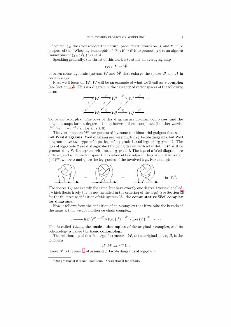
First we’ll focus on W . W will be an example of what we’ll call an ι-complex
(see Section 3.7). This is a diagram in the category of vector spaces of the followingform:
0 / / W 0d0 / /
ι0
~ ~ ~ ~ ~ ~ ~ ~
W 1d1 / /
ι1
W 2
ι2
d2 / / . . .
0 / / W
0
ι
d0ι
/ / W
1
ι
d1ι
/ / W
2
ι
d2ι
/ /. . .
To be an ι-complex: The rows of this diagram are co-chain complexes, and thediagonal maps form a degree −1 map between these complexes (in other words,ιi+1 di = −di−1
ι ιi, for all i ≥ 0).The vector spaces W i are generated by some combinatorial gadgets that we’ll
call Weil diagrams. Weil diagrams are very much like Jacobi diagrams, but Weildiagrams have two types of legs: legs of leg-grade 1, and legs of leg-grade 2. Thelegs of leg-grade 2 are distinguished by being drawn with a fat dot. W i will begenerated by Weil diagrams with total leg-grade i. The legs of a Weil diagram areordered, and when we transpose the position of two adjacent legs, we pick up a sign(−1)xy, where x and y are the leg-grades of the involved legs. For example:
= = − in W 6.
The spaces W iι are exactly the same, but have exactly one degree 1 vertex labelledι which floats freely (i.e. is not included in the ordering of the legs). See Section 3for the full precise definition of this system W : the commutative Weil complex
for diagrams.Now it follows from the definition of an ι-complex that if we take the kernels of
the maps ι, then we get another co-chain complex:
0 / / Ker
ι0 d0 / / Ker
ι1 d1 / / Ker
ι2 d2 / / . . .
This is called W basic, the basic subcomplex of the original ι-complex, and itscohomology is called the basic cohomology.
The relationship of this “enlarged” structure, W , to the original space, B, is thefollowing:
H i(W basic) ∼= Bi,
where Bi is the space1 of symmetric Jacobi diagrams of leg-grade i.
1Our grading of B is non-traditional. See Section 2 for details.
8/3/2019 Andrew Kricker- Non-Commutative Chern-Weil Theory and the Combinatorics of Wheeling
be an example of an ι-complex, and χW will be a “map of ι-complexes”.
In Section 5, W will be defined in exactly the same way as W , but withoutintroducing the leg transposition relations. So the relationship of W to W willbe analogous to the relationship between a tensor algebra T (V ), and a symmetricalgebra S (V ) over some vector space V .
The way that this structure enlarges A is a bit different to the way that W enlarges B. In Section 8.2 we’ll see that we can introduce some relations to obtain:
∞i=0
W i
/(relns.) ∼= A ⊕ . . .
The general flow of this work is:
• To show that χW descends to a genuine isomorphism of the basic cohomol-
ogy rings of W and W .
• To show that the usual statement of wheeling is recovered from this factwhen we pass to the “smaller” structures A and B.
1.3. The origins of this work in Alekseev-Meinrenken’s Non-commutative
Chern-Weil theory. This work originated in a course given by E. Meinrenken atthe University of Toronto in the Spring of 2003 in which Alekseev and Meinrenken’swork on a Non-commutative Chern-Weil theory was introduced [ML]. See [M] fora short review of the theory, [AM] for the original paper, and [AM05] for laterdevelopments.
The goal of this work is a self-contained reconstruction and exploration of theirtechnology in the combinatorial setting of the Jacobi diagrams of Quantum Topol-ogy. Before beginning that discussion in the next section, we’ll give here a very brief sketch of the outlines of classical Chern-Weil theory. A more detailed discussionof how our combinatorial definitions fit into the classical picture will be given inSection 3.9, once those definitions have been made.
So let G be a compact Lie group with Lie algebra g. Chern-Weil theory is atheory of characteristic classes in de Rham cohomology of smooth principal G-bundles. Recall that every smooth principal G-bundle arises as a smooth manifoldP with a free smooth left G-action.
What is a characteristic class? The first thing to say is that it is a choice, forevery principal G-bundle P , of a class w(P ) in the cohomology of the base space,B = P/G, which is functorial with respect to bundle morphisms. To be precise: if there is a morphism of principal G-bundles P and P ′, which means that there isa G-equivariant map f : P → P ′, then it should be true that f ∗B(w(P ′)) = w(P ),where f B denotes the map induced by f between the base spaces f B : B → B′.
Chern-Weil theory constructs such systems of classes in de Rham cohomology inthe following way.
(1) It takes an arbitrarily chosen connection form A ∈ Ω1(P ) ⊗ g.(2) It uses it to construct closed forms in Ω(P )basic ⊂ Ω(P ). This is the ring of
basic differential forms on P . It is most simply introduced as the isomorphicimage under π∗ of Ω(B). It is a crucial fact in the theory that this basicsubring is selected as the kernel of a certain Lie algebra of differential op-erators arising from the generating vector fields of the G-action. The main
8/3/2019 Andrew Kricker- Non-Commutative Chern-Weil Theory and the Combinatorics of Wheeling
task of the theory is to canonically construct forms from A lying in thekernel of this Lie algebra. (See Section 3.9 for a more detailed discussion).
(3) It then shows that the cohomology classes in H dR(B) so constructed donot depend on the choice of connection and do indeed have the requiredfunctoriality with repsect to bundle morphisms.
The heart of the Chern-Weil construction is an algebraic structure called the
Weil complex. The Weil complex is based on the graded algebra S (g∗ ⊕g∗) (that
is, the graded symmetric algebra on two copies of g∗, the dual of g, one copy in grade1 and one copy in grade 2). The Weil complex is this graded algebra equipped witha certain graded Lie algebra of graded derivations. This Lie algebra of derivationsselects a key subalgebra S (g∗ ⊕ g
∗)basic, the basic subalgebra.What is the construction then? Consider some principal G-bundle P . Given the
fixed data of a connection form A ∈ Ω1(P ) ⊗ g on P , Chern-Weil theory constructsa map
It is immediate in the theory that this construction specializes to a map of differ-ential graded algebras from the basic subalgebra of the Weil complex into the ringof basic forms on P :
S (g∗ ⊕ g∗)basic → Ω(P )basic
∼= Ω(B),
so that, passing to cohomology, we get a map:
H ∗ (S (g∗ ⊕ g∗)basic) → H ∗dR(B).
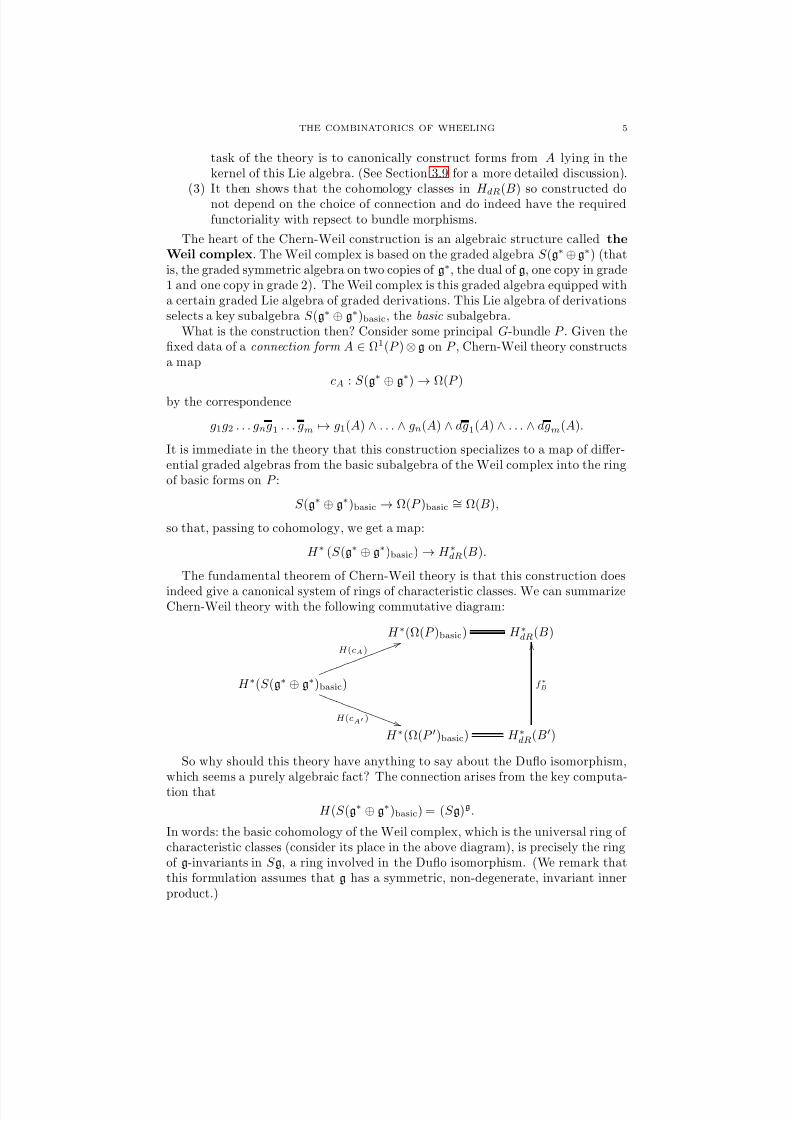
The fundamental theorem of Chern-Weil theory is that this construction does
indeed give a canonical system of rings of characteristic classes. We can summarizeChern-Weil theory with the following commutative diagram:
H ∗(Ω(P )basic) H ∗dR(B)
H ∗(S (g∗ ⊕ g∗)basic)
H (cA) 5 5 k k k k k k k k k k k k k k
H (cA′ ) ) ) S S
S S S S S S
S S S S S S
H ∗(Ω(P ′)basic) H ∗dR(B′)
f ∗B
O O
So why should this theory have anything to say about the Duflo isomorphism,which seems a purely algebraic fact? The connection arises from the key computa-tion that
H (S (g∗ ⊕ g∗)basic) = (S g)g.
In words: the basic cohomology of the Weil complex, which is the universal ring of characteristic classes (consider its place in the above diagram), is precisely the ringof g-invariants in S g, a ring involved in the Duflo isomorphism. (We remark thatthis formulation assumes that g has a symmetric, non-degenerate, invariant innerproduct.)
8/3/2019 Andrew Kricker- Non-Commutative Chern-Weil Theory and the Combinatorics of Wheeling
1.4. A Weil complex for diagrams. This paper will start with a combinatorialreconstruction of that key computation
H (S (g∗ ⊕ g∗)basic) = (S g)g
.Recall that when we abstract Wheeling from the Duflo isomorphism, we replace(S g)g by B, the space of symmetric Jacobi diagrams. An evaluation map (theobvious, minor variation on the “weight system” construction, [B]) connects thetwo: Evalg : B → (S g)g.
We’ll begin by replacing the “something” in the following equation
H ((Something)basic) = B,
by an appropriate construction: W , the commutative Weil complex for diagrams.The complex W is a combinatorial version of the usual Weil complex S (g∗ ⊕ g
∗).Because the usual Weil complex is built from two copies of g∗, one in grade 1 andone in grade 2, W will be built from diagrams with two types of legs: legs of grade1 and legs of grade 2. In other words,
W will be generated by the “Weil diagrams”
introduced in Section 1.2.The full details of the construction of W will be presented in Section 3. W will
be constructed to be an ι-complex, so that we may take its basic cohomology.The final ingredient required in the explication of the equation H i(W basic) ∼= Bi
is the map
Υ : B → W
which actually performs the isomorphism. This map Υ occupies a key role inour presentation. It will be introduced in Section 4, where the computation thatH (W basic) = B will be concluded. Its definition on some symmetric Jacobi diagramw is quite simple: choose an ordering of the legs of w, then expand each leg accordingto the following rule:
Υ : → − 12 .
Sometimes we’ll refer to Υ as the hair-splitting map.
1.5. Some motivation for a non-commutative Weil complex. As the authorlearnt it from E. Meinrenken, this construction can be motivated with the followingline of thought: to begin, note that there is almost a much more natural way tobuild these characteristic classes in de Rham cohomology. The more natural waywould exploit EG, the classifying bundle of principal G-bundles, and its associatedbase space EG/G = BG. Recall the key property of EG that the bundle pullbackoperation performs a bijection, for some space X :
Isomorphism classes of principal G-bundles over X ↔ [X : BG].
So, proceeding optimistically, we could define the ring of characteristic classes as-sociated to some smooth principal G-bundle P by the map:
Class∗P : H dR(BG) → H dR(B),
for some choice of classifying map ClassP : B → BG giving P as its correspondingpullback bundle. This ring would be well-defined because the map ClassP is unique
8/3/2019 Andrew Kricker- Non-Commutative Chern-Weil Theory and the Combinatorics of Wheeling
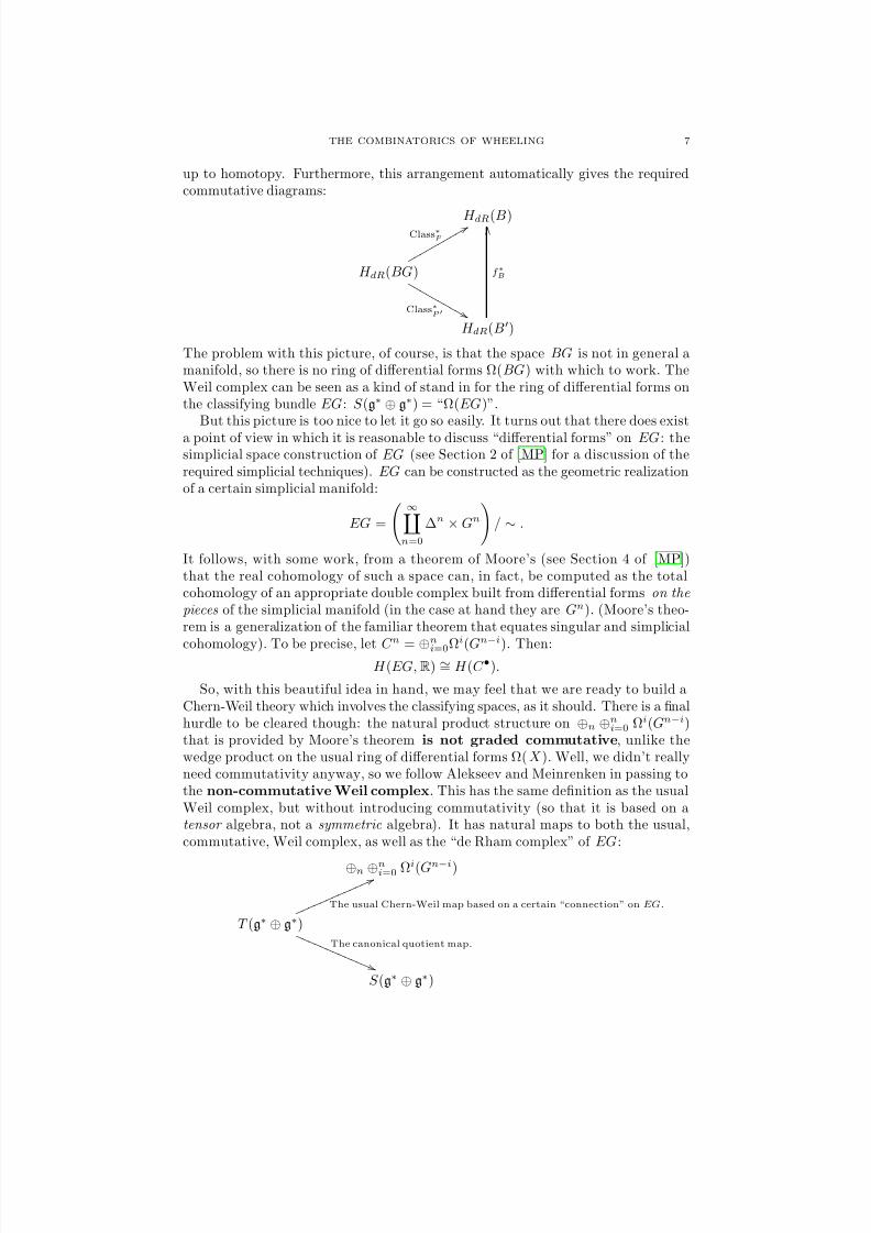
up to homotopy. Furthermore, this arrangement automatically gives the requiredcommutative diagrams:
H dR(B)
H dR(BG)
Class∗P
8 8 q q q q q q q q q q
Class∗P ′ & & M
M M M M
M M M M
M
H dR(B′)
f ∗B
O O
The problem with this picture, of course, is that the space BG is not in general amanifold, so there is no ring of differential forms Ω(BG) with which to work. TheWeil complex can be seen as a kind of stand in for the ring of differential forms onthe classifying bundle EG: S (g∗ ⊕ g
∗) = “Ω(EG)”.But this picture is too nice to let it go so easily. It turns out that there does exist
a point of view in which it is reasonable to discuss “differential forms” on EG: thesimplicial space construction of EG (see Section 2 of [MP] for a discussion of therequired simplicial techniques). EG can be constructed as the geometric realizationof a certain simplicial manifold:
EG =
∞n=0
∆n × Gn
/ ∼ .
It follows, with some work, from a theorem of Moore’s (see Section 4 of [MP])that the real cohomology of such a space can, in fact, be computed as the totalcohomology of an appropriate double complex built from differential forms on thepieces of the simplicial manifold (in the case at hand they are Gn). (Moore’s theo-rem is a generalization of the familiar theorem that equates singular and simplicial
cohomology). To be precise, let C n
= ⊕n
i=0Ωi
(Gn−i
). Then:H (EG,R) ∼= H (C •).
So, with this beautiful idea in hand, we may feel that we are ready to build aChern-Weil theory which involves the classifying spaces, as it should. There is a finalhurdle to be cleared though: the natural product structure on ⊕n ⊕ni=0 Ωi(Gn−i)that is provided by Moore’s theorem is not graded commutative, unlike thewedge product on the usual ring of differential forms Ω(X ). Well, we didn’t reallyneed commutativity anyway, so we follow Alekseev and Meinrenken in passing tothe non-commutative Weil complex. This has the same definition as the usualWeil complex, but without introducing commutativity (so that it is based on atensor algebra, not a symmetric algebra). It has natural maps to both the usual,commutative, Weil complex, as well as the “de Rham complex” of EG:
⊕n ⊕ni=0 Ωi(Gn−i)
T (g∗ ⊕ g∗)
The usual Chern-Weil map based on a certain “connection” on EG.
6 6 m m m m m m m m m m m m m
The canonical quotient map.
( ( Q Q Q Q
Q Q Q Q
Q Q Q Q
Q
S (g∗ ⊕ g∗)
8/3/2019 Andrew Kricker- Non-Commutative Chern-Weil Theory and the Combinatorics of Wheeling
The Alekseev-Meinrenken proof of the Duflo isomorphism arises from an algebraicstudy of the relationship between the two Weil complexes, T (g∗⊕g
∗) and S (g∗⊕g∗),
exploiting properties of T (g∗ ⊕ g∗) that derive from its place as the universal ring
in a characteristic class theory.
1.6. The Non-commutative Weil complex for Diagrams. So in Section 5 we
define W , a non-commutative Weil complex for diagrams, in the way that will be
obvious at this point of the development. The interplay between W and W is atthe heart of this theory. There are two natural maps between these ι-complexes:
W
χW ) ) W
τ
i i .
The map χW is a key map: the graded averaging map. Its action on some Weildiagram w is to take the average of all diagrams you can get by rearranging thelegs of w (each multiplied by a sign appropriate to the rearrangement). The map τ
is the basic quotient map (corresponding to the introduction of the commutativityrelations).
Caution: Our combinatorial analogue of the “non-commutative Weil complex”
defined by the work [AM] is actually a quotient of this complex W by a certain
system of relations. The precise corresponding structure we use, W F, will be dis-
cussed later, in Section 8.5. This complex W is the analog of a deeper (and simpler)structure that was discovered in the later work [AM05].
1.7. Homological Wheeling. When we compose Υ, the “Hair-splitting map”,with χW , the graded averaging map, we get a map which takes elements of B to
basic cohomology classes in W :
BΥ
−→ W basicχW−→ W basic.
So if we take two elements v and w of B, then (χW Υ) (v ⊔ w) represents a basic
cohomology class in W basic.
But there is another way to build a basic cohomology class in W basic from v and
w, using the juxtaposition product # on W . This is a product on basic cohomologyarising from the following product defined on the generating diagrams:
# = .
Theorem 1.7.1 (Homological Wheeling). Let v and w be elements of B. Then the
two elements of
W basic:
• (χW Υ) (v ⊔ w)• (χW Υ) (v)# (χW Υ) (w)
represent the same basic cohomology class.
The technical fact which underlies Homological Wheeling is that the two maps
from the basic subcomplex of W to itself:
W basic
χWτ , ,
id 2 2 W basic
8/3/2019 Andrew Kricker- Non-Commutative Chern-Weil Theory and the Combinatorics of Wheeling
are chain homotopic. The homotopy is constructed in Section 7. In words: if z ∈
W
represents some basic cohomology class, then its graded symmetrization representsthe same basic cohomology class. In the case at hand, this fact implies that:
(χW Υ) (v)# (χW Υ) (w)
and
(χW τ ) ((χW Υ) (v)# (χW Υ) (w)) = (χW Υ) (v ⊔ w)
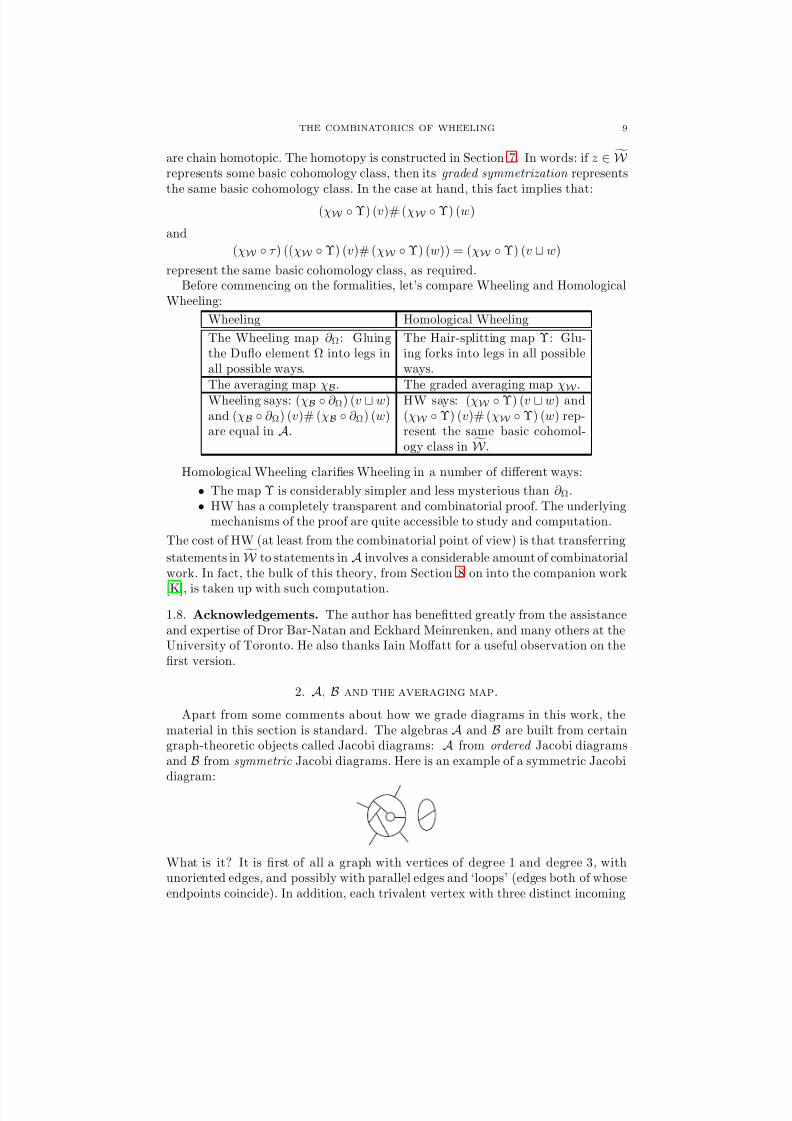
represent the same basic cohomology class, as required.Before commencing on the formalities, let’s compare Wheeling and Homological
Wheeling:
Wheeling Homological Wheeling
The Wheeling map ∂ Ω: Gluingthe Duflo element Ω into legs inall possible ways.
The Hair-splitting map Υ: Glu-ing forks into legs in all possibleways.
The averaging map χB. The graded averaging map χW .Wheeling says: (χB ∂ Ω) (v ⊔ w)and (χB ∂ Ω) (v)# (χB ∂ Ω) (w)are equal in A.
HW says: (χW Υ) (v ⊔ w) and(χW Υ) (v)# (χW Υ) (w) rep-resent the same basic cohomol-ogy class in W .
Homological Wheeling clarifies Wheeling in a number of different ways:
• The map Υ is considerably simpler and less mysterious than ∂ Ω.• HW has a completely transparent and combinatorial proof. The underlying
mechanisms of the proof are quite accessible to study and computation.
The cost of HW (at least from the combinatorial point of view) is that transferring
statements in
W to statements in A involves a considerable amount of combinatorial
work. In fact, the bulk of this theory, from Section 8 on into the companion work
[K], is taken up with such computation.
1.8. Acknowledgements. The author has benefitted greatly from the assistanceand expertise of Dror Bar-Natan and Eckhard Meinrenken, and many others at theUniversity of Toronto. He also thanks Iain Moffatt for a useful observation on thefirst version.
2. A, B and the averaging map.
Apart from some comments about how we grade diagrams in this work, thematerial in this section is standard. The algebras A and B are built from certaingraph-theoretic objects called Jacobi diagrams: A from ordered Jacobi diagramsand B from symmetric Jacobi diagrams. Here is an example of a symmetric Jacobidiagram:
What is it? It is first of all a graph with vertices of degree 1 and degree 3, withunoriented edges, and possibly with parallel edges and ‘loops’ (edges both of whoseendpoints coincide). In addition, each trivalent vertex with three distinct incoming
8/3/2019 Andrew Kricker- Non-Commutative Chern-Weil Theory and the Combinatorics of Wheeling
edges has an orientation (a cyclic ordering of its incident edges). To read the orien-tation of a vertex from a drawing of a symmetric Jacobi diagram (as above) simplytake the counter-clockwise ordering determined by the drawing. Two symmetricJacobi diagrams are isomorphic if there is an isomorphism of their underlyinggraphs which respects the orientations at the trivalent vertices.
Definition 2.0.1. The space B is defined to be the rational vector space obtained by quotienting the vector space of formal finite rational linear combinations of iso-morphism classes of symmetric Jacobi diagrams by its subspace generated by theanti-symmetry (AS) and Jacobi (IHX) relations:
AS : + = 0.
IHX : − − = 0.
We remark that the relation which sets a diagram featuring a loop to be zerowill be considered an instance of an AS relation.
Next let’s consider the space A. An ordered Jacobi diagram is the same asa symmetric Jacobi diagram but has an extra piece of structure: the set of verticesof degree 1 has been ordered.
Definition 2.0.2. The space A is defined to be the rational vector space obtained by quotienting the vector space of formal finite rational linear combinations of iso-morphism classes of ordered Jacobi diagrams by its subspace generated by the anti-symmetry (AS), Jacobi (IHX) and permutation (STU) relations:
STU : − − = 0 .
There is a natural map between these vector spaces, the averaging map2 χB,which was already recalled in Section 1.2. The proof of the following statement canbe read in [B]:
The formal Poincare-Birkhoff-Witt theorem. The averaging map is a vector space isomorphism.
These spaces have natural product structures. The product on A (we’ll refer toit as the “juxtaposition product”) looks like
# = .
2Remark: in this work we require averaging maps between a variety of different spaces. To
keep the notation logical we will record the domain space as a subscript on the symbol χ.
8/3/2019 Andrew Kricker- Non-Commutative Chern-Weil Theory and the Combinatorics of Wheeling
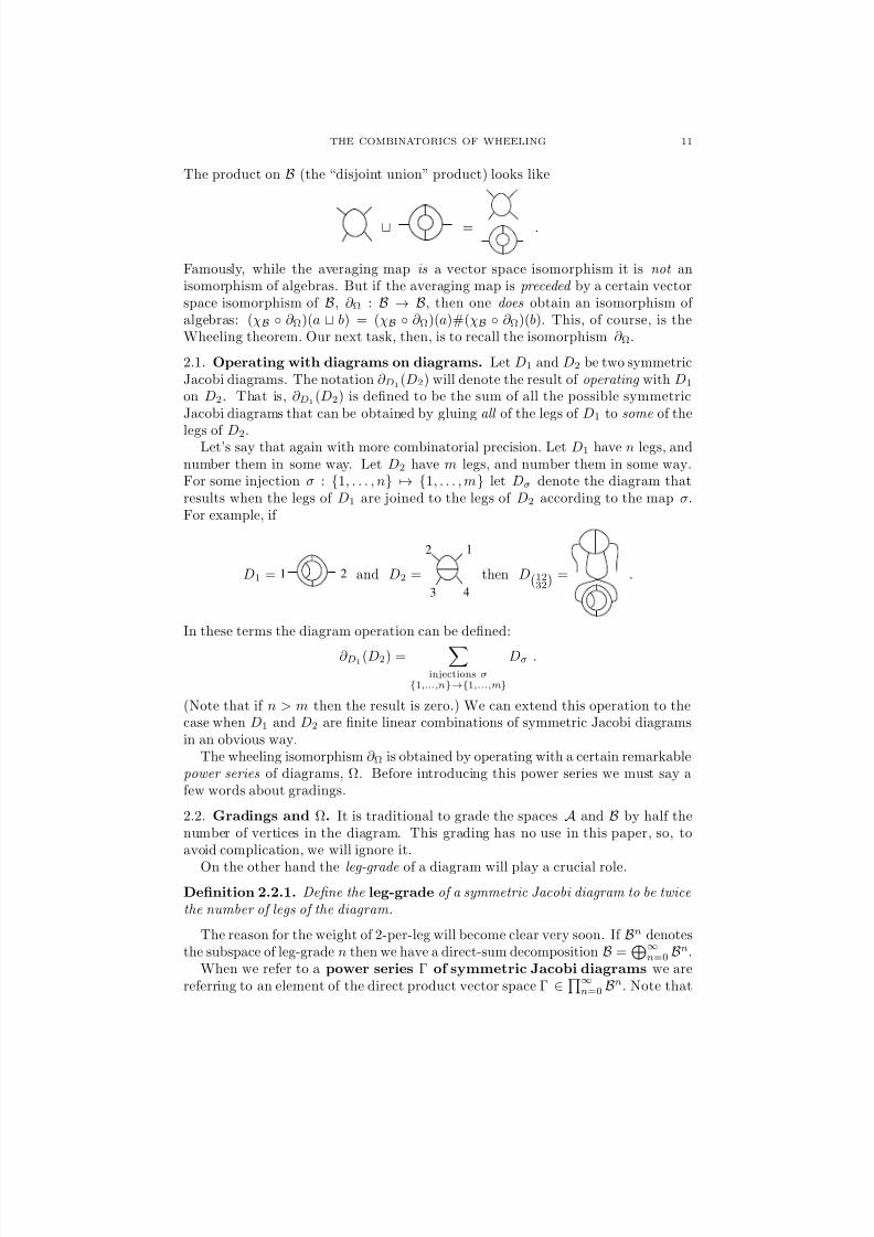
The product on B (the “disjoint union” product) looks like
⊔ = .
Famously, while the averaging map is a vector space isomorphism it is not anisomorphism of algebras. But if the averaging map is preceded by a certain vectorspace isomorphism of B, ∂ Ω : B → B, then one does obtain an isomorphism of algebras: (χB ∂ Ω)(a ⊔ b) = (χB ∂ Ω)(a)#(χB ∂ Ω)(b). This, of course, is theWheeling theorem. Our next task, then, is to recall the isomorphism ∂ Ω.
2.1. Operating with diagrams on diagrams. Let D1 and D2 be two symmetricJacobi diagrams. The notation ∂ D1
(D2) will denote the result of operating with D1
on D2. That is, ∂ D1(D2) is defined to be the sum of all the possible symmetric
Jacobi diagrams that can be obtained by gluing all of the legs of D1 to some of the
legs of D2.Let’s say that again with more combinatorial precision. Let D1 have n legs, and
number them in some way. Let D2 have m legs, and number them in some way.For some injection σ : 1, . . . , n → 1, . . . , m let Dσ denote the diagram thatresults when the legs of D1 are joined to the legs of D2 according to the map σ.For example, if
D1 = 21 and D2 =4
12
3
then D(1232) = .
In these terms the diagram operation can be defined:
∂ D1(D2) =
injections σ1,...,n→1,...,m
Dσ .
(Note that if n > m then the result is zero.) We can extend this operation to thecase when D1 and D2 are finite linear combinations of symmetric Jacobi diagramsin an obvious way.
The wheeling isomorphism ∂ Ω is obtained by operating with a certain remarkablepower series of diagrams, Ω. Before introducing this power series we must say afew words about gradings.
2.2. Gradings and Ω. It is traditional to grade the spaces A and B by half thenumber of vertices in the diagram. This grading has no use in this paper, so, toavoid complication, we will ignore it.
On the other hand the leg-grade of a diagram will play a crucial role.
Definition 2.2.1. Define the leg-grade of a symmetric Jacobi diagram to be twicethe number of legs of the diagram.
The reason for the weight of 2-per-leg will become clear very soon. If Bn denotesthe subspace of leg-grade n then we have a direct-sum decomposition B =
∞n=0 Bn.
When we refer to a power series Γ of symmetric Jacobi diagrams we arereferring to an element of the direct product vector space Γ ∈
∞n=0 Bn. Note that
8/3/2019 Andrew Kricker- Non-Commutative Chern-Weil Theory and the Combinatorics of Wheeling
if Γ is such a power series, then we get a well-defined map ∂ Γ : B → B because allbut finitely many of the terms of Γ contribute zero.
To introduce Ω we will employ a notation that gets used in disparate works inthe literature. If we draw a diagram, orient an edge of the diagram at some point,and label that point with a power series in some formal variable a, then:
c0 + c1a + c2a2 + c3a3 + . . .
denotes c0 + c1 + c2 + c3 + . . . .
Definition 2.2.2. The Wheels element, Ω, is the formal power series of symmetricJacobi diagrams defined by the expression
Ω = exp⊔
1
2( )
a2
a2
( )sinhln
∈∞n=0
Bn .
The combinatorial mechanisms that produce this element are the main subjectof the companion work [K].
3. The commutative Weil complex for diagrams
The purpose of this section is the introduction of a certain cochain complexW basic. The next section will describe a certain map of cochain complexes (with
the spaces Bi assembled into a complex with zero differential), Υibasic : Bi → W ibasic,which gives isomorphisms in cohomology3:
H i(Υbasic) : Bi ∼= H i(B)∼=
−→ H i(W basic).
Our goal is a clean presentation of the combinatorial constructions. These con-structions may appear quite mysterious at first glance, however, so to provide somecontext to the theory, we’ll close the section by constructing a “characteristic class-valued evaluation map”. Given the data of a compact Lie group G, a smoothprincipal G-bundle P with corresponding base B = P \G, and a connection form
A on P , we’ll construct a map of complexes Eval(G,P,A) : W → Ω(P ) (this mapevaluates Weil diagrams in Ω(P )) which yields a map
H Eval(G,P,A)basic : B ∼= H (W basic) → H (Ω(P )basic) ∼= H dR(B).
3.1. Weil diagrams. The distinguishing feature of Weil diagrams is that their legsare graded . Every leg of a Weil diagram is either of grade 1 or of grade 2. The grade2 legs are distinguished by drawing them with a fat dot. The leg-grade of a Weildiagram is the total grade of the legs. Thus, the following example has leg-grade 6:
3A remark concerning our notation: if f is a chain map between cochain complexes then H (f )
(or sometimes H i(f )) will denote the induced map on cohomology.
8/3/2019 Andrew Kricker- Non-Commutative Chern-Weil Theory and the Combinatorics of Wheeling
The precise definition of Weil diagram is unsurprising: it is a graph withvertices of degree 1 and 3, where each degree 3 vertex is oriented, and the set of degree 1 vertices U is ordered and weighted by a grading U → 1, 2.
Occasionally a “Weil diagram with a special degree 1 vertex” is used, whichis just a Weil diagram except that exactly one of the degree 1 vertices is neitherincluded in the total ordering nor assigned a leg-grading.
3.2. Permuting the legs of Weil diagrams. When constructing spaces fromthese diagrams, we’ll always employ the familiar AS and IHX relations. The nu-merous spaces we employ will differ from each other according to how they treatthe legs of the diagrams. As there are really quite a number of different sets of
relations applied to legs in this work we’ll remind the reader of which space weare in by drawing the arrow on the orienting line in a different style depending onwhich space the diagram is in.
To begin: consider relations which say that we are allowed to move the legsaround freely, as long as when we transpose an adjacent pair of legs we introducethe sign (−1)xy, where x and y are the grades of the two legs involved:
Perm1 : − = 0
Perm2 : − = 0
Perm3 : + = 0
Definition 3.2.1. The vector space W i is defined to be the quotient of the vector space of formal finite Q-linear combinations of isomorphism classes of Weil dia-grams of leg-grade i by the subspace generated by AS, IHX and Perm relations. If i < 0 then W i is understood to be zero.
3.2.2. A clarification concerning W 0. We regard the empty diagram as a Weil di-
agram. Thus, for example,
1
2−
7
6
is an element of W 0.To assemble these vector spaces into a complex we first need to learn how to
operate on them with “differential operators”.
8/3/2019 Andrew Kricker- Non-Commutative Chern-Weil Theory and the Combinatorics of Wheeling
3.3. Formal linear differential operators. A formal linear differential operatorof grade j is a sequence D0, D1, . . . of linear maps Di : W i → W i+j defined bya pair of substitution rules. The substitution rules are specified by the followingdata: X , a Weil diagram of leg-grade j + 1 with a special degree 1 vertex, and Y ,a Weil diagram of leg-grade j + 2 with a special degree 1 vertex. More generally X and Y can be formal finite combinations of such diagrams.
Given w, a Weil diagram of leg-grade i, the evaluation of Di(w) begins by placinga copy of the word “D(” on the far left-hand end of the base vector and a copy of the symbol “)” on the far right-hand end of the base vector. The word “D(” is thenpushed towards the “)” by the repeated application of the two substitution rules:
( D
X
+ (−1)1j
( D
,
D(
Y + (−1)2j
D( .
When the word “D(” reaches the symbol “)” then that diagram is eliminated andthe procedure terminates. In some situations the closing bracket appears earlieralong the orienting line. In the typical situation, when the closing bracket appearson the far-right of the orienting line, we’ll omit the brackets altogether. The readercan check that this operation respects the Perm relations.
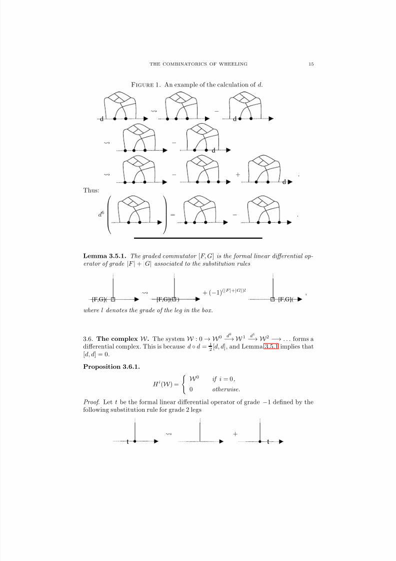
3.4. Example: the differential. Let us illustrate all this by an important specific
example. Define the differential di : W i → W i+1 to be the formal linear differentialoperator of degree +1 corresponding to the following substitution rules:
d
−d
,
d
0 +d
.
Figure 1 gives an example of the calculation of the value of d. Before showing that
this map actually is a differential (i.e. that d d = 0), we’ll record a useful lemma.
3.5. The Lie algebra of formal linear differential operators. Let F and G bea pair of a pair of formal linear differential operators, of grades |F | and |G|. Theirgraded commutator is defined by [F, G] = F G − (−1)|F ||G|G F . The followinglemma (whose proof is a formal exercise in the definitions) says that [ F, G] is again a formal linear differential operator.
8/3/2019 Andrew Kricker- Non-Commutative Chern-Weil Theory and the Combinatorics of Wheeling
together with the rule that says that t graded-commutes through grade 1 legs:
t 0 −
tIt follows from Lemma 3.5.1 that [t, d](D) = (# of legs of D) D, where D is anarbitrary Weil diagram. So for every i > 0 define a map si : W i → W i−1 by
si(D) =1
(# of legs of D)ti(D).
This is the required contracting homotopy: di−1 si+si+1 di = idi, when i ≥ 1.
So the complex W has trivial cohomology. There is, however, a subcomplex of W ,the basic subcomplex W basic, whose cohomology spaces are canonically isomorphicto the Bi (as will be discussed in Section 4). To cut out the subcomplex W basic ⊂W , we need a simple structure we’ll call an ι-complex.
3.7. ι-complexes. An ι-complex is a pair of complexes together with a grade −1map ι between them. Our first ι-complex, to be defined presently, looks like this:
0 / / W 0d0 / /
ι0
~ ~ ~ ~ ~ ~ ~ ~
W 1d1 / /
ι1
W 2
ι2
d2 / / . . .
0 / / W 0ιd0ι / / W 1ι
d1ι / / W 2ι
d2ι / / . . .
To be precise: the equations di+1 di = 0, di+1ι diι = 0 and ιi+1 di = −di−1
ι ιi
hold in the above system. (This last equation has a (−1) because d is grade 1 andι is grade −1.)
Definition 3.7.1. The basic subcomplex Kbasic associated to an ι-complex
(K, Kι, ι) is defined by setting Kibasic = Ker(ιi) and by defining the differential to bethe restriction of the differential on K. (The rule that ι commutes with d impliesthat this actually is a subcomplex. )
Definition 3.7.2. A map f : (K, Kι, ιK) → (L, Lι, ιL) between a pair of ι-complexesis just a pair of sequences of maps ( f i : Ki → Li, f iι : Kiι → Liι ) commuting with the d’s and the ι’s. (Commuting up to sign as determined by the understanding that d and dι are regarded as grade 1 maps, f and f ι as grade 0 maps, and ι as a grade −1 map.)
A map f : (K, Kι, ιK) → (L, Lι, ιL) between ι-complexes restricts to a chain mapbetween their basic subcomplexes. The restriction will be denoted
f basic : Kbasic → Lbasic.
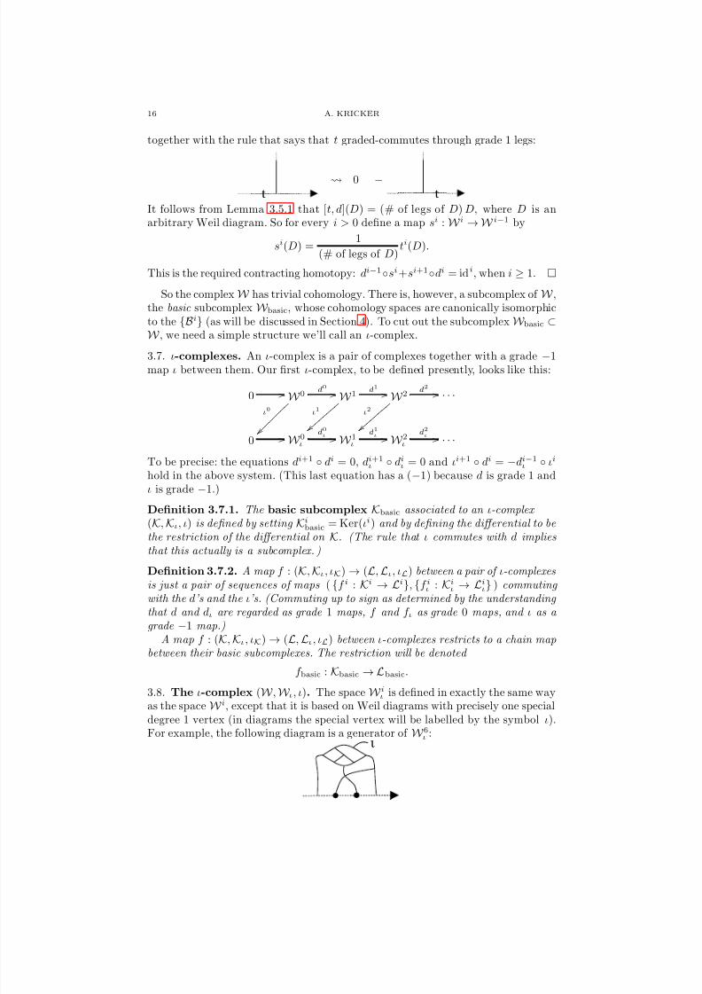
3.8. The ι-complex (W , W ι, ι). The space W i
ι is defined in exactly the same wayas the space W i, except that it is based on Weil diagrams with precisely one specialdegree 1 vertex (in diagrams the special vertex will be labelled by the symbol ι).For example, the following diagram is a generator of W 6ι :
ι
8/3/2019 Andrew Kricker- Non-Commutative Chern-Weil Theory and the Combinatorics of Wheeling
The map ι is the formal linear differential operator of grade −1 defined by thesubstitution rules:
ι
ι−
ι,
ι
ι +ι
.
Proposition 3.8.1. With these definitions, (W , W ι, ι) forms an ι-complex.
Proof. The only remaining thing to verify is that [ι, d] = 0. Lemma 3.5.1 tellsus that [ι, d] is the formal linear differential operator associated to the following
substitution rule (the leg in the box can be of either type):
[ι, ]d
ι +d[ι, ]
This operator is precisely zero on W . To see why this is true we’ll examine itsaction on a generic Weil diagram. To begin:
d[ι, ]= ι + ι
= ι .
The box above represents the sum over all ways of placing the end of the ι-labellededge on one of the edges going through the box. Then we can just use the AS andIHX relations to “sweep” the box up and off the diagram:
ι
(IHX)=
ι (IHX)=
ι
(IHX)= . . .
(IHX)=
ι
(AS)= 0.
8/3/2019 Andrew Kricker- Non-Commutative Chern-Weil Theory and the Combinatorics of Wheeling
So the triple (W , W ι, ι) forms an ι-complex. Thus we can pass to the basicsubcomplex W basic. The computation of the corresponding basic cohomology is thesubject of Section 4.
3.9. The characteristic class-valued evaluation map. The most commonlyasked question that arises when this formalism is described is: what is the ι for?
As we discussed in the introduction, these structures start as a formal abstractionof expressions inside Chern-Weil theory. In this section we’ll make the relationshipmore precise, explaining how to ‘evaluate’ Weil diagrams inside the de Rham com-plex on a principal bundle, so as to build characteristic classes.
So consider a compact Lie group G and a smooth manifold P with a free, smoothleft G-action. It turns out that the space of orbits P/G, which we’ll denote B, maybe uniquely equipped with the structure of a smooth manifold so that P , B andthe projection map π : P → B form a smooth principal G-bundle. Indeed, it turnsout that every smooth principal G-bundle arises in this fashion.
The Chern-Weil theory of characteristic classes begins by examining the corre-sponding pull-back map of differential forms π∗ : Ω(B) → Ω(P ) and asking: isthis map an injection of graded differential algebras? If so, can we characterize theimage of this map? Yes, and yes, are the answers.
The characterization requires the generating vector fields of the G-action onP . Let g denote the Lie algebra of G. Given a vector ξ ∈ g, the vector of thecorresponding generating vector field ξP at a point p of P is given by the derivative:
(ξP f ) ( p) =d
dtf (exp(−tξ) .p)
t=0
.
There are two graded differential operators on Ω(P ) that are naturally associatedto a generating vector field ξP :
• Lξ : Ω•(P ) → Ω•(P ), the Lie derivative along ξP ,• ιξ : Ω•(P ) → Ω•−1(P ), the corresponding contraction operator. Given τ , a
1-form on P , ιξ simply evaluates τ on the vector field ξP . In other words,(ιξτ ) ( p) = τ p((ξP ) p).
Fact. The graded differential operators Lξ, ιξ and d satisfy the following graded commutation relations:
Consider, now, some differential form ω on B, and consider its pull-back π∗(ω)to P . Our first observation is that any such pull-back has the property that it isannihilated by every L
ξand also by every ι
ξ. Before noting the simple reasons for
this fact, let’s encode it in a definition:
Definition 3.9.1. A differential form on P is said to be basic if it is annihilated by every Lξ and also by every ιξ. Let Ω(P )basic denote the ring of basic forms.
Proposition 3.9.2. The pull-back map π∗ maps into the ring of basic forms:
π∗(Ω(B)) ⊂ Ω(P )basic.
8/3/2019 Andrew Kricker- Non-Commutative Chern-Weil Theory and the Combinatorics of Wheeling
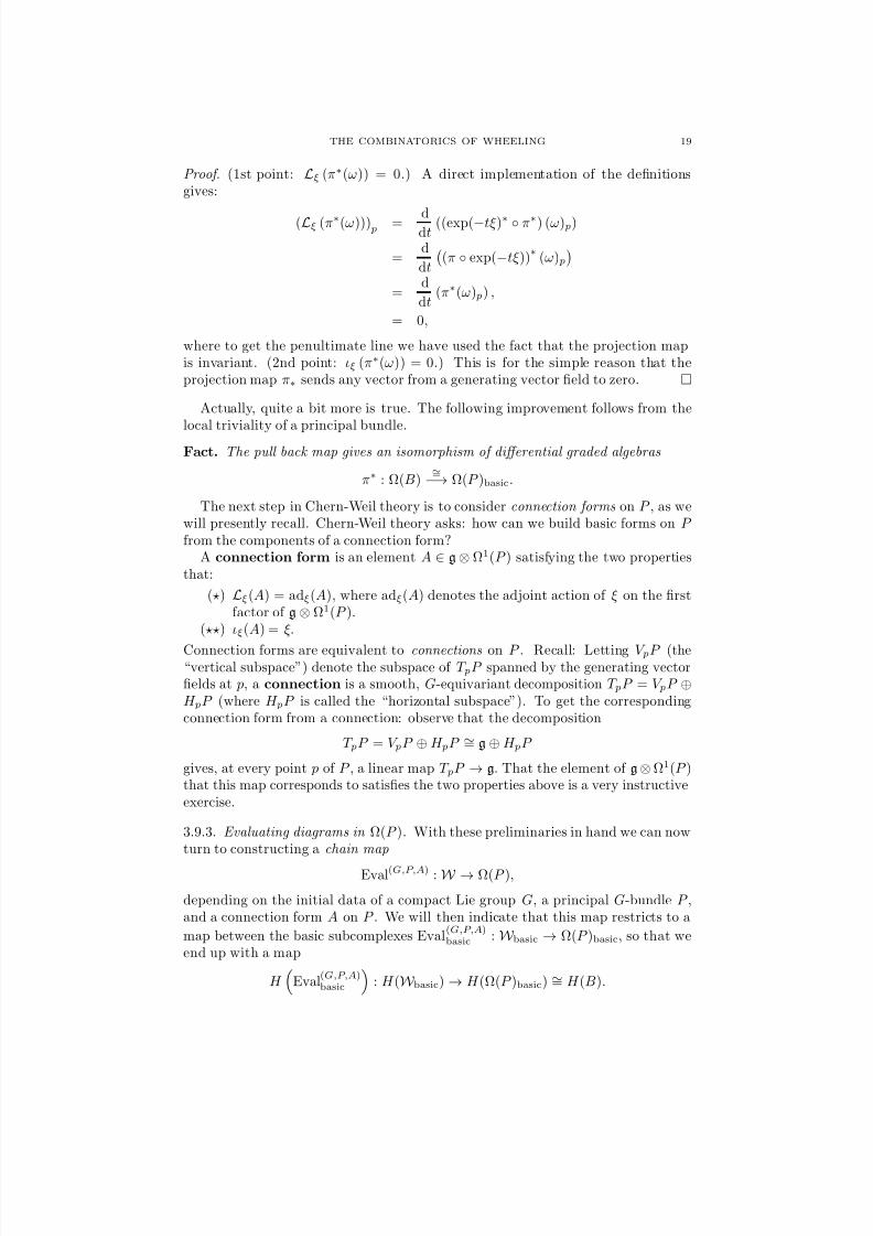
Proof. (1st point: Lξ (π∗(ω)) = 0.) A direct implementation of the definitionsgives:
(Lξ (π∗(ω))) p
= ddt
((exp(−tξ)∗ π∗) (ω) p)
=d
dt
(π exp(−tξ))
∗(ω) p
=
d
dt(π∗(ω) p) ,
= 0,
where to get the penultimate line we have used the fact that the projection mapis invariant. (2nd point: ιξ (π∗(ω)) = 0.) This is for the simple reason that theprojection map π∗ sends any vector from a generating vector field to zero.
Actually, quite a bit more is true. The following improvement follows from thelocal triviality of a principal bundle.
Fact. The pull back map gives an isomorphism of differential graded algebras
π∗ : Ω(B)∼=
−→ Ω(P )basic.
The next step in Chern-Weil theory is to consider connection forms on P , as wewill presently recall. Chern-Weil theory asks: how can we build basic forms on P from the components of a connection form?
A connection form is an element A ∈ g ⊗ Ω1(P ) satisfying the two propertiesthat:
(⋆) Lξ(A) = adξ(A), where adξ(A) denotes the adjoint action of ξ on the firstfactor of g ⊗ Ω1(P ).
(⋆⋆) ιξ(A) = ξ.
Connection forms are equivalent to connections on P . Recall: Letting V pP (the“vertical subspace”) denote the subspace of T pP spanned by the generating vectorfields at p, a connection is a smooth, G-equivariant decomposition T pP = V pP ⊕H pP (where H pP is called the “horizontal subspace”). To get the correspondingconnection form from a connection: observe that the decomposition
T pP = V pP ⊕ H pP ∼= g ⊕ H pP
gives, at every point p of P , a linear map T pP → g. That the element of g⊗ Ω1(P )that this map corresponds to satisfies the two properties above is a very instructiveexercise.
3.9.3. Evaluating diagrams in Ω(P ). With these preliminaries in hand we can nowturn to constructing a chain map
Eval(G,P,A) : W → Ω(P ),
depending on the initial data of a compact Lie group G, a principal G-bundle P ,and a connection form A on P . We will then indicate that this map restricts to a
map between the basic subcomplexes Eval(G,P,A)basic : W basic → Ω(P )basic, so that we
end up with a map
H
Eval(G,P,A)basic
: H (W basic) → H (Ω(P )basic) ∼= H (B).
8/3/2019 Andrew Kricker- Non-Commutative Chern-Weil Theory and the Combinatorics of Wheeling
We will refer to this map as the characteristic class-valued evaluation map.The computation of H (W basic), the “universal ring” in this characteristic classtheory, is the subject of the next section. (The answer is B.)
The map Eval(G,P,A) will be constructed as a state-sum in the familiar way. Forcompleteness, we’ll describe the method in detail here. To begin, let’s fix somenotation to refer to three important tensors associated to the initial data.
(1. The inner product .) The Lie algebra g, being the Lie algebra of a compactLie group, comes equipped with an inner product which is:
(1) Symmetric, so that v, w = w, v;(2) Invariant, so that [u, v], w + v, [u, w] = 0;(3) Non-degenerate, so that the map from g to g
∗ given by v → v, . is anisomorphism. Let : g∗ → g denote the inverse map.
(2. The Casimir element .) The identity map from g to itself can be viewed asan element of g∗ ⊗ g. (In coordinates: introduce a basis taa=1..dimg. Let t∗adenote the set of dual vectors defined by the rule t∗a(tb) = δab. Then the identity
map is a t∗a ⊗ ta.) If we take the tensor representing the identity map and apply to the first factor (what physicists call “lowering the index”) then we get a tensor
in g ⊗ g which we’ll refer to as the Casimir element. Write this element as a suma sa ⊗ ta.(3. The connection form .) The connection form A is an element of g ⊗ Ω1(P ).
Write it as a sum: A =i ri ⊗ ωi.
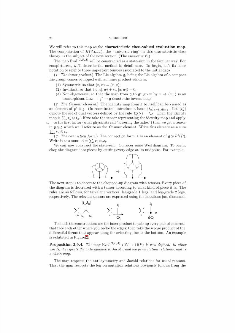
We can now construct the state-sum. Consider some Weil diagram. To begin,chop the diagram into pieces by cutting every edge at its midpoint. For example:
→
The next step is to decorate the chopped-up diagram with tensors. Every piece of the diagram is decorated with a tensor according to what kind of piece it is. Therules are as follows, for trivalent vertices, leg-grade 1 legs, and leg-grade 2 legs,respectively. The relevant tensors are expressed using the notations just discussed.
a,b
a sb
ta
tb[ , ]
s
i
ωi
ri i
d
i
ωi
r
To finish the construction: use the inner product to pair up every pair of elementsthat face each other where you broke the edges; then take the wedge product of the
differential forms that appear along the orienting line at the bottom. An exampleis exhibited in Figure 2.
Proposition 3.9.4. The map Eval(G,P,A) : W → Ω(P ) is well-defined. In other words, it respects the anti-symmetry, Jacobi, and leg permutation relations, and isa chain map.
The map respects the anti-symmetry and Jacobi relations for usual reasons.That the map respects the leg permutation relations obviously follows from the
8/3/2019 Andrew Kricker- Non-Commutative Chern-Weil Theory and the Combinatorics of Wheeling
grading of the differential forms involved in the state-sum. It is a chain map byconstruction.
Proposition 3.9.5. The map Eval(G,P,A) restricts to a map
Eval(G,P,A)basic : W basic → Ω(P )basic
between the basic subcomplexes.
We’ll leave the proof as an instructive exercise. The reader needs to check thata form in the image of this map is annihilated by every Lξ and by every ιξ . In thecase of Lξ: first observe the effect that the degree 0 differential operator Lξ has on
an expression like shown in Figure 2 above. Then use the defining property (⋆) of a connection to convert that expression an appropriate diagrammatic expression.Finish with a sweeping argument. For the case of ιξ: use the defining property (⋆⋆)of a connection to show that the result of the action by ιξ must factor through thediagrammatic ι.
4. Introducing the map Υ.
In this section we’ll see how to map B, the familiar space of symmetric Jacobidiagrams, into W , the just-introduced commutative Weil complex for diagrams, inorder to get isomorphisms in basic cohomology:
H i(Υbasic) : Bi ∼= H i(Bbasic)∼=
−→ H i(W basic).
We’ll introduce Υ as the composition of two other maps of ι-complexes:
(B, 0, 0)φB
−−−→ (W F, W Fι, ι)BF→•−−−−→ (W , W ι, ι).
Formally speaking, this section will be rather routine. We’ll introduce the ι-complex(W F, W Fι, ι). Then we’ll introduce the maps BF→• and φB
4. Along the way we’llexplain that they both induce isomorphisms in basic cohomology.
4There is a B suffix in this notation to logically distinguish this map from a later A version
φA.
8/3/2019 Andrew Kricker- Non-Commutative Chern-Weil Theory and the Combinatorics of Wheeling
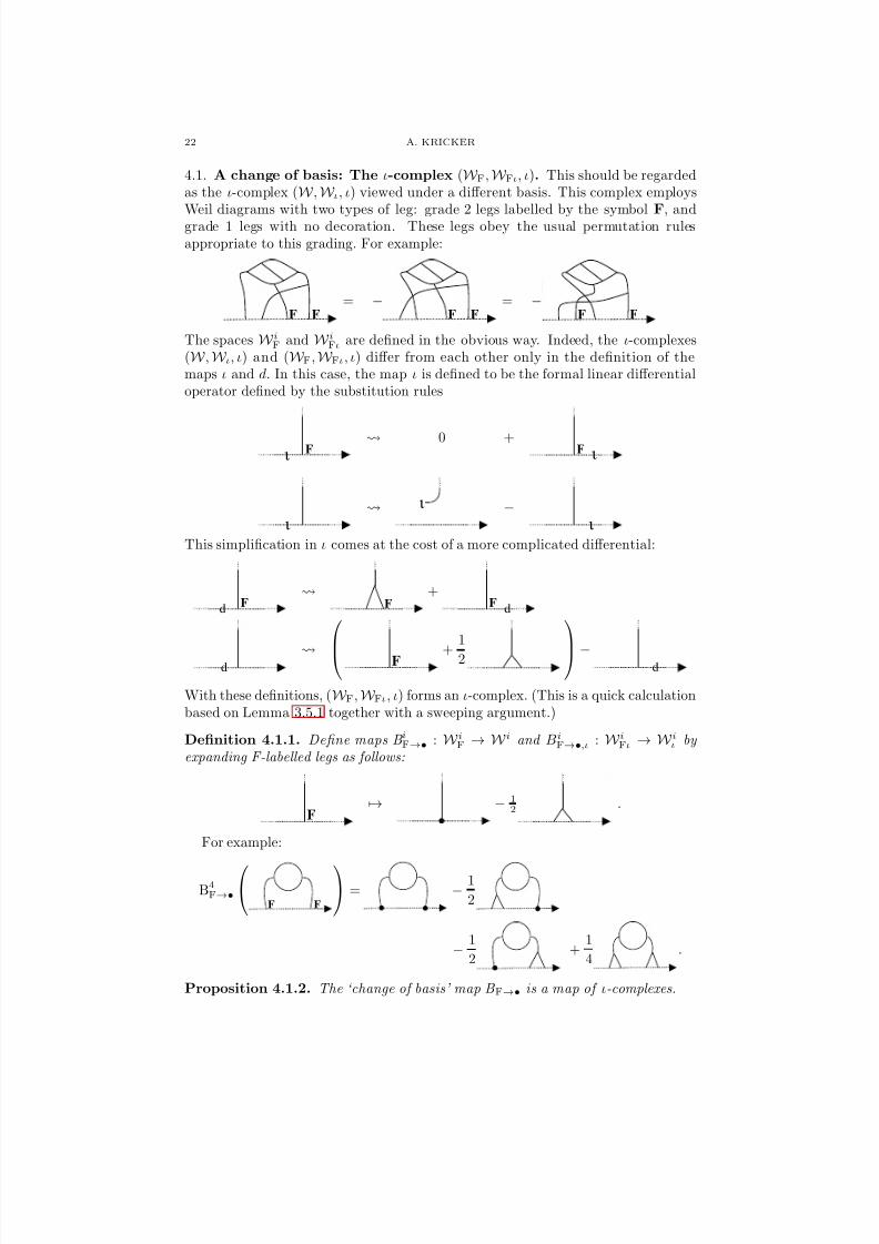
4.1. A change of basis: The ι-complex (W F, W Fι, ι). This should be regardedas the ι-complex (W , W ι, ι) viewed under a different basis. This complex employsWeil diagrams with two types of leg: grade 2 legs labelled by the symbol F, andgrade 1 legs with no decoration. These legs obey the usual permutation rulesappropriate to this grading. For example:
FF= −
FF= −
FF
The spaces W iF and W iFι are defined in the obvious way. Indeed, the ι-complexes(W , W ι, ι) and (W F, W Fι, ι) differ from each other only in the definition of themaps ι and d. In this case, the map ι is defined to be the formal linear differentialoperator defined by the substitution rules
ι F 0 +
F ι
ι
ι −ι
This simplification in ι comes at the cost of a more complicated differential:
d F
F+
dF
d
F +
1
2 −d
With these definitions, (W F, W Fι, ι) forms an ι-complex. (This is a quick calculationbased on Lemma 3.5.1 together with a sweeping argument.)
Definition 4.1.1. Define maps B iF→• : W iF → W i and BiF→•,ι : W iFι → W iι by expanding F-labelled legs as follows:
F→ − 1
2 .
For example:
B4F→•
F F
= −1
2
−1
2+
1
4.
Proposition 4.1.2. The ‘change of basis’ map B F→• is a map of ι-complexes.
8/3/2019 Andrew Kricker- Non-Commutative Chern-Weil Theory and the Combinatorics of Wheeling
We begin by assembling the spaces Bi into an ι-complex in the following way (re-calling that symmetric Jacobi diagrams are graded by 2-per-leg):
0 / / B0 0 / /
0
~ ~ ~ ~ ~ ~ ~ ~
0 0 / /
0
~ ~ ~ ~ ~ ~ ~ ~
B2 0 / /
0
~ ~ ~ ~ ~ ~ ~ ~
0 0 / /
0
~ ~ ~ ~ ~ ~ ~ ~
B4
0
~ ~ ~ ~ ~ ~ ~ ~
0 / / 0 0 / /
0
| | | | | | | | |
. . .
00 / / 0
0 / / 00 / / 0
0 / / 00 / / 0
0 / / . . .
Note the obvious fact that
H i(Bbasic) =
Bi if i is even,
0 if i is odd.
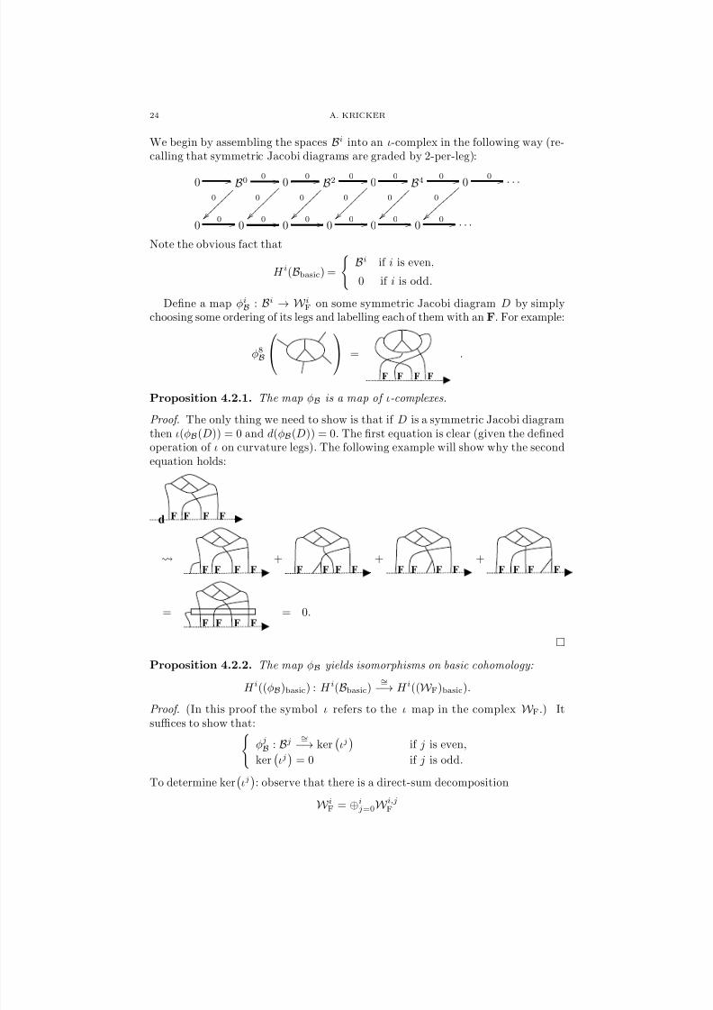
Define a map φiB : Bi → W iF on some symmetric Jacobi diagram D by simplychoosing some ordering of its legs and labelling each of them with an F. For example:
φ8B =
FF F F
.
Proposition 4.2.1. The map φB is a map of ι-complexes.
Proof. The only thing we need to show is that if D is a symmetric Jacobi diagramthen ι(φB(D)) = 0 and d(φB(D)) = 0. The first equation is clear (given the definedoperation of ι on curvature legs). The following example will show why the secondequation holds:
Fd F F F
FF F F+
FF F F+
FF F F+
FF F F
=FF F F
= 0.
Proposition 4.2.2. The map φB yields isomorphisms on basic cohomology:
H i((φB)basic) : H i(Bbasic)∼=
−→ H i((W F)basic).
Proof. (In this proof the symbol ι refers to the ι map in the complex W F.) Itsuffices to show that:
φjB : Bj∼=
−→ ker
ιj
if j is even,
ker
ιj
= 0 if j is odd.
To determine ker
ιj
: observe that there is a direct-sum decomposition
W iF = ⊕ij=0W i,jF
8/3/2019 Andrew Kricker- Non-Commutative Chern-Weil Theory and the Combinatorics of Wheeling
where W i,jF is the subspace generated by Weil diagrams with exactly j grade 1legs. This direct-sum decomposition exists because there are no relations involvingdiagrams with varying numbers of such legs. Note that W i,0 is obviously isomorphicto Bi.
The proposition follows immediately from the claim that ker(ιi) = W i,0F . Note
that it is immediate from the action of ι on F-labelled legs that ker(ιi) ⊃ W i,0F .
To prove that ker(ιi) ⊂ W i,0F , let ιi : W i−1Fι → W iF be the map which takes the
special ι-labelled leg and places it at the far left hand end of the orienting line. Forexample:
ι6
ι
F F
=
FF
Observe that (ιi ιi)(D) = jD , if D ∈ W i,jF . Thus ker(ιi) ⊂ ker(ιi ιi) = W i,0,
establishing the claim.
To summarize: If we define maps Υi by the composition Υi = BiF→• φiB, thenPropositions 4.1.3 and 4.2.2 give us the following theorem.
Theorem 4.2.3. The induced maps H i(Υbasic) : Bi ∼= H i(Bbasic) → H i(W basic)are isomorphisms.
5. The non-commutative Weil complex.
In this section we embed the commutative Weil complex for diagrams into alarger ι-complex, the non-commutative Weil complex for diagrams:
χW : (W , W ι, ι) → (
W ,
W ι, ι).
This larger complex is built in the same way as W but without introducing thepermutation relations; the embedding χW is the graded averaging map. The keytechnical theorem regarding this ι-complex says, in essence, that every cocycle z inW basic has its corresponding basic cohomology class [z] represented by its gradedsymmetrisation (χW τ ) (z).
Definition 5.0.4. Define vector spaces W i in exactly the same way as the vector spaces W i but without introducing the permutation relations.
For the purposes of clarity, we’ll always draw generators of W , which we’ll referto as non-commutative Weil diagrams, with a certain arrow head on theirorienting lines. Observe:
= = − in W 6.
Define d, W ι, and ι in the obvious way. These definitions form an ι-complex (thecalculation that [d, ι] = 0 is exactly the same here as it is for W , Lemma 3.8.1).
The basic subcomplex here seems much harder to construct explicitly than it isin the commutative case. It is a startling and central fact, however, that the two
8/3/2019 Andrew Kricker- Non-Commutative Chern-Weil Theory and the Combinatorics of Wheeling
ι-complexes have canonically isomorphic basic cohomology spaces. We’ll show thisby constructing a chain equivalence of ι-complexes:
W χW ) ) W τ
i i .
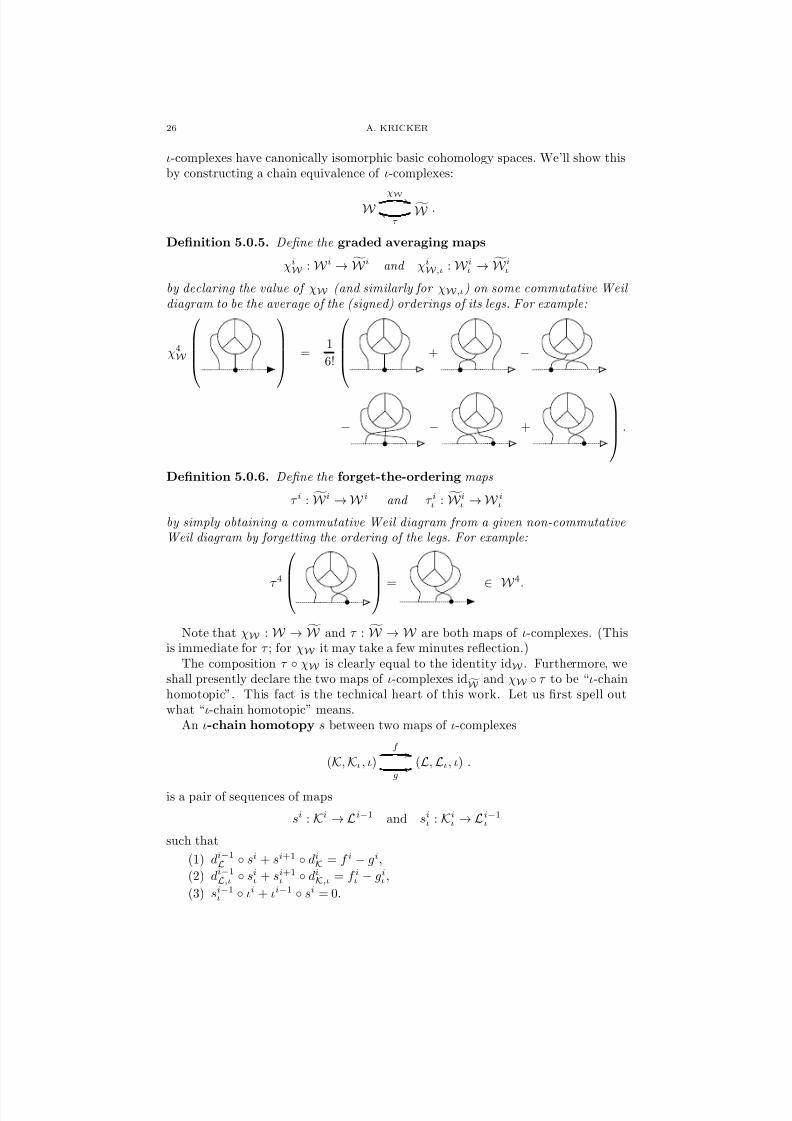
Definition 5.0.5. Define the graded averaging maps
χiW : W i → W i and χiW ,ι : W iι → W iι
by declaring the value of χW (and similarly for χW ,ι) on some commutative Weil diagram to be the average of the (signed) orderings of its legs. For example:
χ4W
=1
6!
+ −
− − +
.
Definition 5.0.6. Define the forget-the-ordering maps
τ i : W i → W i and τ iι : W iι → W iι
by simply obtaining a commutative Weil diagram from a given non-commutativeWeil diagram by forgetting the ordering of the legs. For example:
τ
4 = ∈ W
4
.
Note that χW : W → W and τ : W → W are both maps of ι-complexes. (Thisis immediate for τ ; for χW it may take a few minutes reflection.)
The composition τ χW is clearly equal to the identity idW . Furthermore, weshall presently declare the two maps of ι-complexes idW
and χW τ to be “ι-chainhomotopic”. This fact is the technical heart of this work. Let us first spell outwhat “ι-chain homotopic” means.
An ι-chain homotopy s between two maps of ι-complexes
(K, Kι, ι)
f - -
g 1 1 (L, Lι, ι) .
is a pair of sequences of maps
si : Ki → Li−1 and siι : Kiι → Li−1ι
such that
(1) di−1L si + si+1 diK = f i − gi,
(2) di−1L,ι siι + si+1
ι diK,ι = f iι − giι ,
(3) si−1ι ιi + ιi−1 si = 0.
8/3/2019 Andrew Kricker- Non-Commutative Chern-Weil Theory and the Combinatorics of Wheeling
It will not surprise the reader to learn that if two maps of ι-complexes are ι-chainhomotopic, then the induced maps on the basic subcomplexes
Kbasic
f basic , ,
gbasic
2 2 Lbasic
are chain homotopic.
Theorem 5.0.7 (The key technical theorem). There exists an ι-chain homotopy
s : W → W
between the two maps of ι-complexes id W and χW τ .
The construction of this ι-chain homotopy is the subject of Section 7.
6. Homological wheeling
In this section we will state the Homological Wheeling (HW) theorem, and pointout why it is an immediate consequence of the existence of the ι-chain homotopydescribed in Theorem 5.0.7. In Section 7 that chain homotopy will be constructed,and in Section 8 we’ll explain how the usual Wheeling theorem is recovered fromHW when certain relations are introduced.
6.1. The statement. First we’ll make some comments concerning the ingredientsof HW. In Section 4.2 we showed how to take symmetric Jacobi diagrams (i.e.generators of B) and construct basic cocycles in W . Recall this map Υ: orderthe legs of the symmetric Jacobi diagram, label each leg with an F, then expandthese legs into the usual basis. If we continue on and compose Υ with the graded
averaging map χW , then we have constructed basic cocycles in W (because the
graded averaging map is a map of ι-complexes). HW concerns these cocycles.Formalizing this composition:
Definition 6.1.1. Let Hi : Bi → H i(W basic) denote the linear map given by the formula Hi = H i((χ Υ)basic).
The other ingredient in HW is the natural graded product on the ι-complex W .For two non-commutative diagrams D1 and D2, D1#D2 is defined by placing D2
to the right of D1 on the orienting line. For example:
# = .
Observe that d and ι satisfy the graded Leibniz rule with repsect to this product,so that this product descends to a product on the basic cohomology.
Homological Wheeling. Let v be an element of Bi and w be an element of Bj.Then:
Hi+j(v ⊔ w) = Hi(v)#Hj(w) ∈ H i+j(W basic).
It is worth re-expressing this theorem in more concrete terms.
8/3/2019 Andrew Kricker- Non-Commutative Chern-Weil Theory and the Combinatorics of Wheeling
6.2. The error term. Here we’ll make a brief comment about how the error termin the above statement - d(xv,w) - fits into the big picture. When we introducerelations to recover Wheeling (as described in Section 8) we’ll use the knowledgethat ι(xv,w) = 0 to show that that term vanishes. This is more-or-less the reasonwe have to carry information about the action of the map ι through the calculation.
6.3. How Theorem 5.0.7 implies HW. Consider the left-hand side of the equa-tion stated in Theorem 6.1.2: (χW Υ)(v)#(χW Υ)(w). If we insert this elementinto the equation idW = χW τ + s d + d s, then we learn that it is equal to
(χW τ ) ((χW Υ)(v)#(χW Υ)(w)) + d (s ((χW Υ)(v)#(χW Υ)(w))) ,
where we have used the fact that (χW Υ)(v)#(χW Υ)(w) is a cocycle in W .It takes but a moment to agree that
(χW τ ) ((χW Υ)(v)#(χW Υ)(w)) = (χW Υ)(v ⊔ w) ,
and, setting
xv,w = s ((χW Υ)(v)#(χW Υ)(w)) ,
we have the required right-hand side (noting that ι(xv,w) = 0 because s commutes
with ι and (χW Υ)(v)#(χW Υ)(w) is a basic element of W ).
7. The construction of the ι-chain homotopy s.
The construction of the ι-chain homotopy s and the verification of its propertiesis a 100% combinatorial exercize. The combinatorial work takes place in two ι-
complexes T and T dR. The ι-complex T is an intermediary between W and W ,with some legs behaving as if they are in W and some legs behaving as if they are inW . The complex T dR may be viewed as a formal version of the result of tensoringT with the de Rham complex over the interval, which will allow us to mimic aStokes theorem argument combinatorially.
7.1. The ι-complex T . The ι-complex T is based on diagrams of the followingsort, which will be referred to as T -diagrams:
.
In a T -diagram two legs never lie on the same vertical line. Thus the set of legsof a T -diagram is ordered. The rules for permuting the order of legs depend onwhich orienting lines they lie on. If they lie on different orienting lines, or both lieon the bottom (the commutative) orienting line, then they can be permuted, up to
8/3/2019 Andrew Kricker- Non-Commutative Chern-Weil Theory and the Combinatorics of Wheeling
sign, in the usual way. If, however, they both lie on the top (the non-commutative)line, then they cannot be permuted. Thus, in T 7:
= − = − = −
We’ll apply formal linear differential operators to these spaces. To apply a dif-ferential operator one thinks of a vertical line sweeping along the pair of orientinglines. Figure 3 shows an example of the calculation of this differential. The map ι
is defined similarly, and with these definitions (T , T ι, ιT ) forms an ι-complex.Constructions in T can be translated to W by means of a certain map of ι-
complexes ω : (T , T ι, ιT ) → (W , W ι, ιW ).
Definition 7.1.1. The value of the map ω on some T -diagram is constructed in two steps.
(1) Permute (with the appropriate signs) the legs of the diagram so that all thelegs lying on the commutative orienting line lie to the right of all the legs
8/3/2019 Andrew Kricker- Non-Commutative Chern-Weil Theory and the Combinatorics of Wheeling
lying on the non-commutative orienting line. For example:
= − .
(2) Now take the average of all (signed) permutations of the legs on the com-mutative orienting line and adjoin the result to the right-hand end of thenon-commutative orienting line. The example is concluded in Figure 4.
There are two natural maps of ι-complexes from the ι-complex W to the ι-complex T . They are in : W → T , the map which puts all legs of the originaldiagram on the top (non-commutative) line, as in:
i6n
= ,
and ic : W → T , the corresponding map which puts all legs of the original diagramon the bottom (commutative) line. Observe that
χW τ = ω ic and that idW = ω in.
Theorem 7.1.2. There exists an ι-chain homotopy sT : W → T between the twomaps in and ic.
The construction of this ι-chain homotopy is the subject of the next two sub-sections. The key theorem, Theorem 5.0.7, is a quick consequence of it. Therequired ι-homotopy is defined by the formula s = ω sT .
Proof of Theorem 5.0.7 . We must check that this map satisfies the propertiesof an ι-chain homotopy between the maps χW τ and idW . To begin, note that
8/3/2019 Andrew Kricker- Non-Commutative Chern-Weil Theory and the Combinatorics of Wheeling
s commutes with ι. This is because sT commutes with ι (as asserted by Theorem7.1.2) and because ω is a map of ι-complexes. We must also check:
idW − χW τ = ω (in − ic)= ω (d sT + sT d) ,
= d ω sT + ω sT d,
= d s + s d.
To obtain the penultimate line above we used the fact that ω is a map of ι-complexes.
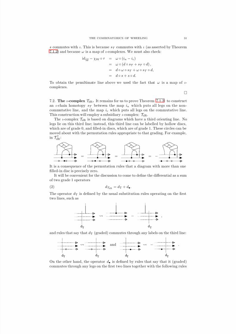
7.2. The ι-complex T dR. It remains for us to prove Theorem 7.1.2: to constructan ι-chain homotopy sT between the map in which puts all legs on the non-commutative line, and the map ic which puts all legs on the commutative line.This construction will employ a subsidiary ι-complex: T dR.
The ι-complex T dR is based on diagrams which have a third orienting line. Nolegs lie on this third line; instead, this third line can be labelled by hollow discs,which are of grade 0, and filled-in discs, which are of grade 1. These circles can bemoved about with the permutation rules appropriate to that grading. For example,in T 7dR:
= = = −
It is a consequence of the permutation rules that a diagram with more than onefilled-in disc is precisely zero.
It will be convenient for the discussion to come to define the differential as a sumof two grade 1 operators
(2) dT dR = dT + d•.
The operator dT is defined by the usual substitution rules operating on the firsttwo lines, such as
Td
−
Td
,
and rules that say that dT (graded) commutes through any labels on the third line:
Td
Td
and
Td
−
Td
.
On the other hand, the operator d• is defined by rules that say that it (graded)commutes through any legs on the first two lines together with the following rules
8/3/2019 Andrew Kricker- Non-Commutative Chern-Weil Theory and the Combinatorics of Wheeling
The map ι is defined by the usual rules for ι applied to the first two lines, togetherwith rules which say that ι (graded) commutes through anything on the third line.We invite the reader to check that, with these definitions, T dR does indeed form anι-complex.
7.3. The construction of the ι-chain homotopy sT . What is this curious com-plex T dR all about then? The empty disc can be thought of as a formal parameter(it may be useful to mentally replace the open discs with the symbol ‘ t’), and thefilled disc is its differential (‘dt’). We chose to use discs to emphasise the fullycombinatorial nature of the manipulations of this section.
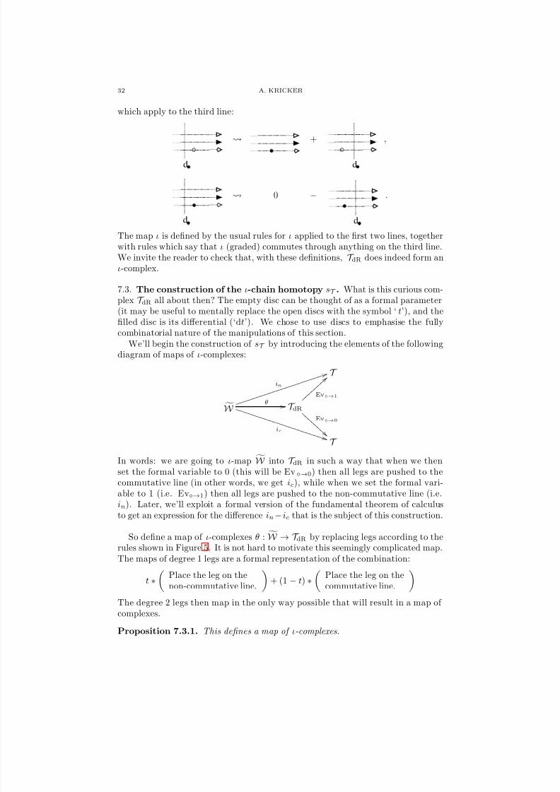
We’ll begin the construction of sT by introducing the elements of the followingdiagram of maps of ι-complexes:
T
W
in
4 4 j j j j j j j j j j j j j j j j j j j j j j
ic
* * T T T T T T
T T T T T T
T T T T T T T T T T
θ / / T dR
Ev→1
> > | | | | | | | |
Ev→0
B B B
B B B B B
T
In words: we are going to ι-map W into T dR in such a way that when we thenset the formal variable to 0 (this will be Ev→0) then all legs are pushed to thecommutative line (in other words, we get ic), while when we set the formal vari-able to 1 (i.e. Ev→1) then all legs are pushed to the non-commutative line (i.e.in). Later, we’ll exploit a formal version of the fundamental theorem of calculusto get an expression for the difference in−ic that is the subject of this construction.
So define a map of ι-complexes θ :
W → T dR by replacing legs according to the
rules shown in Figure 5. It is not hard to motivate this seemingly complicated map.
The maps of degree 1 legs are a formal representation of the combination:
t ∗
Place the leg on thenon-commutative line.
+ (1 − t) ∗
Place the leg on thecommutative line.
The degree 2 legs then map in the only way possible that will result in a map of complexes.
Proposition 7.3.1. This defines a map of ι-complexes.
8/3/2019 Andrew Kricker- Non-Commutative Chern-Weil Theory and the Combinatorics of Wheeling
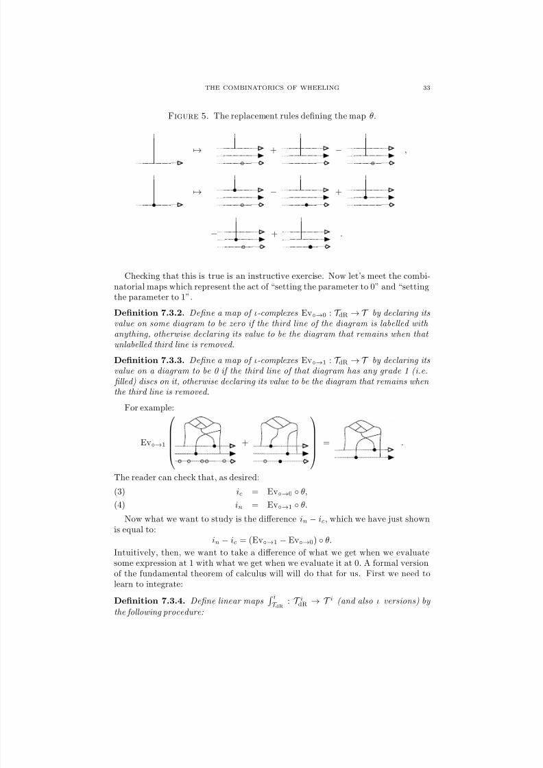
Figure 5. The replacement rules defining the map θ.
→ + − ,
→ − +
− + .
Checking that this is true is an instructive exercise. Now let’s meet the combi-natorial maps which represent the act of “setting the parameter to 0” and “settingthe parameter to 1”.
Definition 7.3.2. Define a map of ι-complexes Ev→0 : T dR → T by declaring itsvalue on some diagram to be zero if the third line of the diagram is labelled with anything, otherwise declaring its value to be the diagram that remains when that unlabelled third line is removed.
Definition 7.3.3. Define a map of ι-complexes Ev→1 : T dR → T by declaring itsvalue on a diagram to be 0 if the third line of that diagram has any grade 1 (i.e.
filled) discs on it, otherwise declaring its value to be the diagram that remains when the third line is removed.
For example:
Ev→1
+
= .
The reader can check that, as desired:
ic = Ev→0 θ,(3)
in = Ev→1 θ.(4)
Now what we want to study is the difference in − ic, which we have just shownis equal to:
in − ic = (Ev→1 − Ev→0) θ.Intuitively, then, we want to take a difference of what we get when we evaluatesome expression at 1 with what we get when we evaluate it at 0. A formal versionof the fundamental theorem of calculus will will do that for us. First we need tolearn to integrate:
Definition 7.3.4. Define linear maps iT dR
: T idR → T i (and also ι versions) by
the following procedure:
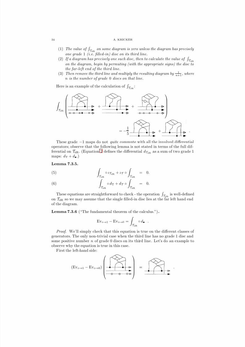
8/3/2019 Andrew Kricker- Non-Commutative Chern-Weil Theory and the Combinatorics of Wheeling
on some diagram is zero unless the diagram has precisely
one grade 1 (i.e. filled-in) disc on its third line.
(2) If a diagram has precisely one such disc, then to calculate the value of T dRon the diagram, begin by permuting (with the appropriate signs) the disc tothe far-left end of the third line.
(3) Then remove the third line and multiply the resulting diagram by 1n+1 , where
n is the number of grade 0 discs on that line.
Here is an example of the calculation of T dR
:
T dR
+ +
= −1
5+ .
These grade −1 maps do not quite commute with all the involved differentialoperators; observe that the following lemma is not stated in terms of the full dif-ferential on T dR. (Equation 2 defines the differential dT dR as a sum of two grade 1maps: dT + d•.)
Lemma 7.3.5. T dR
ιT dR + ιT
T dR
= 0.(5)
T dR
dT + dT T dR
= 0.(6)
These equations are straightforward to check - the operation T dR
is well-definedon T dR so we may assume that the single filled-in disc lies at the far left hand endof the diagram.
Lemma 7.3.6 (“The fundamental theorem of the calculus.”).
Ev→1 − Ev→0 =
T dR
d• .
Proof. We’ll simply check that this equation is true on the different classes of generators. The only non-trivial case when the third line has no grade 1 disc andsome positive number n of grade 0 discs on its third line. Let’s do an example toobserve why the equation is true in this case.
First the left-hand side:
(Ev→1 − Ev→0)
= .
8/3/2019 Andrew Kricker- Non-Commutative Chern-Weil Theory and the Combinatorics of Wheeling
Now consider the right-hand side. Applying d6• to this diagram gives:
− + = 3 .
Thus:
T dR
d•
= 3
T dR
= (3)1
3 .
The reader should not have any difficulties constructing a general argument fromthis example.
Proof of Theorem 7.1.2 . Define the required homotopy sT by the formula
sT =
T dR
θ.
Observe:
in − ic = (Ev→1 − Ev→0) θ, (Eqns. 3 and 4),= T dR d• θ, (Lemma 7.3.6),
= T dR (dT dR − dT) θ, (Eqn. 2),= (
T dR
dT dR θ) − ( T dR
dT θ),
= ( T dR
θ dW ) − (
T dR
dT θ), (Prop. 7.3.1),
= ( T dR
θ dW ) + (dT
T dR
θ), (Eqn. 5),
= sT dW + dT sT .
8. How to obtain Wheeling from Homological Wheeling.
8.1. (d, ι)-pairs. For the remainder of this work we’ll be working with a number of systems without a natural Z-grading, so it will be necessary to adjust our languagea little. Define a (d, ι)-pair to be a pair of vector spaces with maps,
V ι / /d 9 9 V ι dι g g
such that d2 = 0, d2ι = 0 and d ι = −ι d. An ι-complex, such as W , may be
viewed as a (d, ι)-pair in the following way:
⊕∞i=0
W i⊕ι / /⊕di 6 6 ⊕∞
i=0W iι ⊕di
ι h h .
Write W = ⊕∞i=0W i and W ι = ⊕∞
i=0W iι .
8/3/2019 Andrew Kricker- Non-Commutative Chern-Weil Theory and the Combinatorics of Wheeling
8.2. The roadmap. Recall the statement of Homological Wheeling: Given ele-
ments v ∈ Bi and w ∈ Bj, there exists an element xv,w of
W i+j−1 such that
ι(xv,w) = 0 and such that(χW Υ)
i(v)# (χW Υ)
j(w) = (χW Υ)
i+j(v ⊔ w) + d(xv,w) ∈ W i+j .
This statement holds in W , whereas we want a statement in A, the space of or-
dered Jacobi diagrams. Well, the non-commutative space W has no relations whichconcern the legs of diagrams. We can introduce whatever relations we can think of,and see what consequences may be derived. For example, in attempting to derive astatement in A, we could introduce the STU relations (among degree 2 legs), whichis precisely what we will do in the next section:
(7) − = .
To deduce the usual Wheeling Theorem in A, we will take the following route:
W
IntroducingSTU and other
relations.−−−−−−−−−−−−−−→
π
W
Changing tothe “curvatures”
basis.−−−−−−−−−−−−−−−→
B•→F
W F
Symmetrisingthe grade 1
legs.−−−−−−−−−−−−→
λ
W ∧ = A⊕. . . .
The (d, ι)-pair W F is the combinatorial analogue of the complex W G = U g⊗Cl gthat the work [AM] refers to as the “non-commutative Weil complex”. This wasthe first structure discovered in the theory.
8.3. The (d, ι)-pair (
W ,
W ι, d , ι). The maps d and ι play a crucial role in the
statement of HW. But simply introducing the STU relations leaves these maps ill-
defined. So we must introduce a number of other relations at the same time as weintroduce STU, to ensure that the maps d and ι descend to the quotient spaces.
Define W to be the vector space generated by Weil diagrams modulo AS, IHX,the STU relation (Equation 7), and also the following pair of relations:
− = ,
+ = .
Similarly define the vector space W ι.Recall that the STU relation is a formal analogue of the relation in a universal
enveloping algebra which equates a commutator with the corresponding bracket.And note further that the relation just introduced amongst grade 1 legs is a formalanalogue of the defining relation of a Clifford algebra.
Proposition 8.3.1. The maps d and ι descend to the spaces W and W ι. Thus,
quotienting gives a map of (d, ι)-pairs π : (W , W ι, d , ι) → ( W , W ι, d , ι).
8/3/2019 Andrew Kricker- Non-Commutative Chern-Weil Theory and the Combinatorics of Wheeling
8.4. Some clarifications concerning the diagrams in this section. The Weildiagrams generating the spaces introduced in this section will be allowed to havecomponents consisting of closed loops without vertices. (Even though such compo-nents don’t fit into the usual definition of a graph, it is straightforward to set thisgenerality up formally.) The reason we need such generality is that the ‘Cliffordalgebra’ relation may produce such components when applied to the two ends of atrivial chord with two grade 1 legs.5
We remark that this is only a formal device we employ to make our definitionslogically consistent; the expressions that actually arise when a HW statement isinserted into this composition never use such components.
In addition: let Al be constructed in exactly the same way as the space A butwhere we allow the ordered Jacobi diagrams to have components consisting of closedloops without vertices. There are no relations between these components and therest of the graph. Observe that A is obviously a subspace of Al.
8.5. A change of basis: The (d, ι)-pair W F. We’ll now change back to the“curvatures” basis. Here it has the salutary effect of making the two kinds of legs
invisible to each other. To be precise: define W F to be the vector space generatedby F-Weil diagrams taken modulo AS, IHX, and the following three classes of relations:
FF−
FF=
F,
F−
F= 0 ,
+ = .
Similarly define W Fι. If we equip this pair of spaces with maps d and ι using theusual substitution rules for F-Weil diagrams then we have a (d, ι)-pair. (See Section4 for the reason that [d, ι] = 0. And the calculation that d2 = 0 is a little surprising
in this basis, as we invite the reader to see.) Define maps B•→F : W → W F and
B•→F ,ι : W ι → W Fι by expanding grade 2 legs in the usual way:
→F
+1
2.
These maps give a map of (d, ι)-pairs B•→F : ( W , W ι, d , ι) → ( W F, W Fι, d , ι).
8.6. Symmetrizing the grade 1 legs. The final step on our journey to A is to(graded) symmetrize the grade 1 legs. Intuitively speaking, we are just taking a
special choice of basis in W F (and so in W ). Formally: we’ll define new vector
spaces W ∧ and W ∧ι and equip them with “averaging” maps into W F and W Fι.
5A referee alerted the author to this detail.
8/3/2019 Andrew Kricker- Non-Commutative Chern-Weil Theory and the Combinatorics of Wheeling
W i∧ according to the number of grade 1 legs in a diagram.
We’ll locate Al in the grade 0 position of this decomposition: Al∼= W
0
∧. Finally,we’ll show that ker ι = W 0∧
∼= Al.
8.6.1. The vector spaces W ∧ and W ∧ι. Define W ∧ to be the vector space generatedby F-Weil diagrams modulo AS, IHX, STU (amongst F-legs), and the followingtwo classes of relations:
F−
F= 0 ,
+ = 0 .
Define W ∧ι similarly. In these spaces, then, the grade 1 legs may be moved aboutfreely (up to sign).
We remark, as discussed in Section 8.4, that we are formally allowing closed loop
components. In W ∧ there are no relations that involve such components at all.We will not introduce a differential into these spaces. (The reason is that, in W F, when the differential acts on a grade 1 leg, it produces terms with new grade
1 legs. So the action of the differential in the “symmetrized” basis will look verycomplicated.)
We will only define the map ι : W ∧ → W ∧ι. This is defined as a formal lineardifferential operator, in the usual way. The following theorem will be establishedin some detail in Section 8.9:
Theorem 8.6.2. There exist vector space isomorphisms χ∧ : W ∧ → W F and χ∧ι : W ∧ι → W Fι commuting with the action of ι.
The map χ∧ : W ∧ → W F is defined by declaring the value of the map on somediagram to be the average of the terms that can be obtained by doing (signed)permutations of the degree 1 legs of the diagram. χ∧ι is defined similarly. Anexample is shown in Figure 6.
That the maps commute with ι is straightforward. The difficult part of thetheorem is showing that χ∧ is a vector space isomorphism. This will be done byexplicitly constructing an inverse.
Definition 8.6.3. The inverse to χ∧ will be denoted λ :
W F →
W ∧.
Similarly we have λι. This map λ is a crucial map which will be constructed
explicitly later, in Section 8.8. After constructing λ there we’ll go through thedetails of Theorem 8.6.2. For the present we’ll just assume that such maps exist.
8.6.4. Decomposing according to the number of grade 1 legs. Observe that there are
no relations in W ∧ which involve diagrams with differing numbers of the degree 1
legs. Thus the space W ∧ is graded by that quantity. Let W i∧ denote the subspace of W ∧ generated by diagrams which have exactly i grade 1 legs. We have a direct-sum
decomposition into these subspaces: W ∧ =∞i=0 W i∧ . Observe now that there is a
8/3/2019 Andrew Kricker- Non-Commutative Chern-Weil Theory and the Combinatorics of Wheeling
canonical isomorphism (“label every leg with an F”) from Al, the familiar space of ordered Jacobi diagrams (recall the l subscript allows the possibility of closed loop
components), to W 0∧. We’ll denote it φA : Al∼=
−→ W 0∧. For example:
φA
=
FF F F
.
8.6.5. The kernel of ι on
W ∧. Here we will establish that the kernel of the map ι
is precisely the zeroth summand in this decomposition:
(8) ker ι = W 0∧ ⊂ W ∧.
This fact is a consequence of the map ι : W ∧ι → W ∧ that is defined by placingthe special ι-labelled leg on the far left-hand end of the orienting line. Because, for
some generator v ∈ W ∧,
(ι ι) (v) =
Number of
grade 1 legs of v
v ,
an element of W ∧ lies in the kernel of ι if and only if it lies in W 0∧.
8.7. Wheeling - the key lemmas. Now that we have introduced the spacesinvolved, we can turn to the explanation of how Wheeling arises from HW. Recallthe statement of HW: Given elements v ∈ Bi and w ∈ Bj, there exists an element
xv,w of W i+j−1 such that ι(xv,w ) = 0 and such that
(χW Υ)i
(v)# (χW Υ)j
(w) = (χW Υ)i+j
(v ⊔ w) + d(xv,w) ∈ W i+j .
We’ll now take the three summands of this equation and insert them into thecomposition of linear mapsW
π−→ W
B•→F−−−−→ W Fλ
−→ W ∧ ,
so as to produce a statement in W ∧.
8/3/2019 Andrew Kricker- Non-Commutative Chern-Weil Theory and the Combinatorics of Wheeling
To begin, note that each of the three summands lies in the kernel of ιW . Thus,
each of their images under the map (λ B•→F π) lies in the kernel of ιW ∧, which
we know is isomorphic to Al, via the linear isomorphism φA.So we move on to asking: if we pull these elements back to Al, what do weget? The following, crucial, lemma says that we just get The Wheeling Map
composed with the averaging map from B to A ⊂ Al (just as appears in the Wheel-ing Theorem). The proof is a quite involved (but conceptually straightforward)combinatorial calculation which will appear in a separate publication [K].
Lemma 8.7.1. For all x ∈ B ,φ−1A λ B •→F π
((χW Υ) (x)) = (χB ∂ Ω) (x) .
The next lemma is a quick corollary, as will be explained at the end of thissubsection:
Lemma 8.7.2. The element
φ−1A λ B •→F π
((χW Υ) (v)# (χW Υ) (w)) is
equal to (χB ∂ Ω) (v)# (χB ∂ Ω) (w).
Assuming these lemmas, the only thing which stands in the way of the Wheel-ing Theorem is the error term: d(xv,w), where ι(xv,w) = 0. This error term isdispatched by the following lemma.
Lemma 8.7.3. If z ∈ W is such that ιW (z) = 0, then
(B •→F π) ( d(z) ) = 0 ∈ W F.
Proof. We’ll start by establishing a small claim. We claim that if an element w ∈ W F is in the kernel of ιW F, then it can be expressed as a linear combination of
diagrams each of whose legs is an F-labelled leg. The deduction is that:
• λ(w) is in the kernel of ιW ∧(because λ commutes with ι, by Theorem 8.6.2).
• Thus λ(w) lies in W 0∧ (by Equation 8).
• Thus λ(w) is a linear combination of diagrams all of whose legs are F-labelled.
• Thus w = χW ∧(λ(w)) must also consist of entirely-F-labelled diagrams.
This establishes the claim. Then:
(B•→F π) ( d(z) ) = d ((B•→F π) (z))
= d
A combination of diagrams in W F
every leg of which is labelled by an F.
= 0.
The first equality follows because the maps B•→F and π are both maps of (d, ι)-pairs. The second equality follows from the claim that started this proof (notingthat ι ((B•→F π) (z)) = 0). The third equality we leave as an exercize. (Compare
with the proof of Proposition 4.2.1.)
Proof of Lemma 8.7.2 using Lemma 8.7.1. Consider the expression that is thesubject of this lemma. Briefly considering the constructions of the maps B•→F andπ, we realize that we can write it:
φ−1A λ
((B•→F π χW Υ) (v)#(B•→F π χW Υ) (w)) .
Now, just as in the claim used in the proof of Lemma 8.7.3, we observe that becausethe factors (B•→F π χW Υ) (v) and (B•→F π χW Υ) (w) are both in the
8/3/2019 Andrew Kricker- Non-Commutative Chern-Weil Theory and the Combinatorics of Wheeling
kernel of ιW F, they can be expressed using diagrams whose legs are entirely F-legs.
The map λ does not do anything to such diagrams. Thus, the expression can be
written: φ
−1
A λ B•→F π χW Υ (v)# φ
−1
A λ B•→F π χW Υ (w).
8.8. The map λ. The remaining business of this paper is to prove Theorem 8.6.2.This subsection will define maps λ and λι, prove that they are well-defined, andprove that they left-invert the averaging maps: λ χ∧ = idW ∧
and λι χ∧ι = idW ∧ι.
The next and final subsection will combine these facts with the easy facts that χ∧and χ∧ι are surjective, and that ι commutes with the χ∧, to obtain the theorem.
The constructions of λ and λι are quite natural and easily remembered: “gluechords (with certain easily determined signs and coefficients) into the grade 1 legsin all possible ways”.
8.8.1. The formal definition of λ. Consider a diagram w from
W F. Let L⊥(w)
denote the set of grade 1 legs of w. To begin, we’ll explain how to operate with a
two-element subset S of L⊥(w) on w. The resulting term, which will be denotedDS(w), is obtained from w by:
(1) Doing signed permutations to move one of the legs in S until it is adjacentto the other leg.
(2) Then gluing those two legs together and multiplying the result by 12 .
For example, consider the following diagram w, with the elements of its set L⊥(w)enumerated. To illustrate this operation we will calculate D2,4(w). First we dosigned permutations to make leg 2 adjacent to leg 4:
3
F F
1 2 4
2
F F
1 3 4
−
1
F F
3 2 4
.
Then we glue those two legs together, then multiply by 12 . Thus:
D2,4
3
F F
1 2 4
= −1
2
3
F F
1
.
Now we’ll extend this to an action on w of a pairing of the legs of w. The desiredmap λ will then be defined to be a sum over one term for every pairing.
Definition 8.8.2. A pairing of the legs of a diagram w is defined to be a set of mutually disjoint 2-element subsets of L⊥(w). The empty set will be regarded as a
pairing. Let P (w) denote the set of pairings of the diagram w. Define the action of a pairing ℘ = S 1, . . . , S n on the diagram w, denoted D℘(w), to be:
D℘(w) = (DS1 . . . DSn) (w).
Figure 7 gives an example of the action of a pairing on a diagram.For this to give a well-defined operation on diagrams it is necessary that a differ-
ent choice of ordering of the elements of ℘ will yield the same result. It is sufficientto show that the equation (Da,b Dc,d)(w) = (Dc,d Da,b)(w) always holds,
8/3/2019 Andrew Kricker- Non-Commutative Chern-Weil Theory and the Combinatorics of Wheeling
where a,b,c and d are different legs of some diagram w. To show this equation we just have to observe that it is true for all possible arrangements of the positions of these legs. Let’s just check one possibility, where the two pairs are ‘linked’:
da c b
.
Assume that the total grade of the legs between a and c in the above diagram is p, between c and b is q, and between b and d is r. Then the result of applyingDa,b Dc,d to the above diagram is readily calculated to be
(−1)q+1+r(−1) p+q 1
4.
On the other hand, the result of applying (Dc,d Da,b) is
(−1) p+q+1(−1)q+r 1
4,
which is clearly the same thing. Nothing surprising happens in the other cases.
Definition 8.8.3. Define a linear map λ :
W F →
W ∧ by declaring the value of λ
on some diagram w to be λ(w) = ℘∈P(w) D℘(w). Define a map λι similarly.
An example of the result of a full computation is shown in Figure 8.
8.8.4. The map λ respects relations.
Proposition 8.8.5. The map λ is well-defined.
Proof. We must check that λ maps relations to relations. The map λ only ‘sees’ thegrade 1 legs, so our problem is to show that λ maps the ‘Clifford algebra’ relations
8/3/2019 Andrew Kricker- Non-Commutative Chern-Weil Theory and the Combinatorics of Wheeling
Figure 8. An example of the full calculation of λ.
λ
FF
=
FF
+1
2 FF−
1
2 FF+
1
2 FF
+ 12 FF
− 12 FF
+ 12 FF
+1
4 FF−
1
4 FF+
1
4 FF.
to zero. So consider a particular case of these relations, and let D1, D2 and D3
denote the three involved diagrams. For example:
F
D1
+F
D2
−F
D3
.
Identify the sets of grade 1 legs L⊥(D1) and L⊥(D2) in the natural way determinedby the rest of the graph. (So in the above example the 2nd leg of D1 is identifiedwith the third leg of D2.) Thus we can write:
λ(D1 + D2) = ℘∈P(D1)
(D℘(D1) + D℘(D2)) .
We’ll compute the terms of this sum according to the following three possibilitiesfor the pairing ℘. Call the two grade 1 legs that change position in the expressionthe active legs. The other grade 1 legs are called the inactive legs. The grade 2 legscan be ignored completely.
Possibility #1: Neither of the active legs appear in ℘. In this case it is clear that
D℘(D1) + D℘(D2) = 0, using a leg permutation relation in W ∧.
8/3/2019 Andrew Kricker- Non-Commutative Chern-Weil Theory and the Combinatorics of Wheeling
Possibility #2: At least one of the active legs are paired by ℘ with an inactiveleg. In this case, we again have that D℘(D1) + D℘(D2) = 0. To see this, write
D℘ = DS1 . . . Da,i
where a denotes the active leg referred to, and i denotes the inactive leg it is pairedto. Now calculate:
Da,i(D1) = Da,i
ai
=1
2(−1)x ,
where x denotes the total grade of the legs between i and a. Also:
Da,i(D2) = Da,i
i a
=1
2(−1)x+1 .
Possibility #3: The two active legs are paired with each other. Let P a(D1) ⊂P (D1) denote the set of pairings of D1 which pair the two active legs together.There is a bijection r : P a(D1) → P (D3). The map is just to remove the paira1, a2 from the pairing. A quick calculation gives the equation
D℘(D1) + D℘(D2) = Dr(℘)(D3).
Note: this equation is why we need a “ 12 for every chord” in the definition of λ.
8.8.6. The map λ does indeed left-invert χ∧.
Proof. Consider some diagram w with n degree 1 legs. Write the signed average of the grade 1 legs χ∧(w) =
σ∈Permn
wσ, where Permn denotes the set of permuta-tions of the set 1, . . . , n. For example:
If w =F
then w( 1234
1432 ) = −1
4! F.
For each σ, identify the set of grade 1 legs L⊥(wσ) with L⊥(w) using the order of the legs as they appear along the orienting line from left-to-right. Given a pairing℘ ∈ P (w), we’ll show that D℘
σ∈Permn
wσ
= 0 unless ℘ = φ, from which theproposition follows.
To begin, choose some decomposition D℘ = DS1 . . . Dl1,l2. Assuming w.l.o.g.
that l1 < l2, let Perm||n(l1, l2) ⊂ Permn denote the subset of permutations σ with
the property that if σ(x) = l1 and σ(y) = l2 then x < y. Graphically speak-
ing, Perm||n(l1, l2) consists of those permutations where the straight lines ending
at positions l1 and l2 do not cross. Similarly, define PermXn (l1, l2) ⊂ Permn tobe the subset of permutations where they do cross. There is clearly a bijection
ϑ : Perm||n(l1, l2)
∼=−→ PermXn (l1, l2):
ϑ
2
x y
l l1
=
2
yx
l l1
.
8/3/2019 Andrew Kricker- Non-Commutative Chern-Weil Theory and the Combinatorics of Wheeling
The claim now follows from the observation that Dl1,l2(wσ) = −Dl1,l2(wϑ(σ)).
8.9. Proof of Theorem 8.6.2. To prove this theorem we must:
(1) Prove that ι χ∧ = χ∧ι ι.(2) Prove that χ∧ and χ∧ι are surjective.(3) Observe that because λ χ∧ = idW ∧
and λι χ∧ι = idW ∧ι, it follows that
χ∧ and χ∧ι are also injective.
The first fact is a (straightforward if a little bit technical) combinatorial exercise.
Proposition 8.9.1. The maps χ∧ and χ∧ι are surjective.
Proof. This argument will be familiar. Take w, an arbitrary F-Weil diagram.Let w∧ be the same diagram, but regarded as a generator of W ∧. Then:
w − χ∧(w∧) =
A sum of diagrams withless grade 1 legs than w.
.
By induction, w lies in the image of χ∧.
References
[AM] A. Alekseev and E. Meinrenken, The non-commutative Weil algebra , Invent. Math., 139
(2000), 135–172.[AM05] A. Alekseev and E. Meinrenken, Lie theory and the Chern-Weil homomorphism , Ann.
sci. Ec. norm. supr., 38 no2 (2005), 303–338.
[B] D. Bar-Natan, On the Vassiliev knot invariants, Topology 34 (1995) 423–472.[BGRT] D. Bar-Natan, S. Garoufalidis, L. Rozansky and D. Thurston, Wheels, wheeling, and the
Kontsevich integral of the unknot , Israel J. Math. 119 (2000) 217–237.[BLT] D. Bar-Natan, T. Le and D. Thurston, Two applications of elementary knot theory to
Lie algebras and Vassiliev invariants, Geom. Topol. 7 (2003), 1–31.
[D] M. Duflo, Operateurs differentiels bi-invariants sur un groupe de Lie, Ann. Sci. Ecole
Norm. Sup. 10 (1977), 265–288.[GK] S. Garoufalidis and A. Kricker, “A rational non-commutative invariant of boundary
links”, Geom. Topol. 8 (2004), 115–204.[K] A. Kricker, “Differential operators and the Wheels power series”, submitted to Alg. and
Geom. Topol.
[M] E. Meinrenken, Clifford Algebras and the Duflo isomorphism , Proceedings of the ICM2002, Vol. II (Beijing, 2002), 637–642, Higher Ed. Press, Beijing, 2002.
[ML] E. Meinrenken, Group actions on Manifolds, lectures at the University of Toronto, 2003.
[MP] M. Mostow and J. Perchik, Notes on Gelfand-Fuks cohomology and characteristic classes,Proceedings of the eleventh annual holiday symposium, New Mexico State University
(1973), Lectures delivered by R. Bott, pp. 1–126. This was reprinted in Vol. 3 of thecollected works of Raoul Bott.
Division of Mathematical Sciences, School of Physical and Mathematical Sciences,