96
Final Report for ANACOM PUBLIC VERSION Conceptual approach for a mobile BU-LRIC model 22 September 2011 Ref: 15235-384
| Date post: | 20-Feb-2016 |
| Category: |
Documents |
| Upload: | alifatehitqm |
| View: | 212 times |
| Download: | 0 times |
Final Report for ANACOM
PUBLIC VERSION
Conceptual approach for a mobile BU-LRIC model
22 September 2011
Ref: 15235-384

Conceptual approach for mobile BU-LRIC model
Ref: 15235-384 – PUBLIC VERSION
Contents
1 Introduction 1
2 Principles of long-run incremental costing 4
2.1 Competitiveness and contestability 4
2.2 Long-run costs 4
2.3 Incremental costs 5
2.4 Efficiently incurred costs 6
2.5 Costs of supply using modern technology 6
3 Operator issues 8
3.1 Type of operator 8
3.2 Network footprint of operator 15
3.3 Scale of operator 20
4 Technology issues 25
4.1 Modern network architecture 25
4.2 Network nodes 37
4.3 Dimensioning of the network and impact of data traffic 40
5 Service issues 42
5.1 Service set 42
5.2 Traffic volumes 45
5.3 Migration of voice from 2G to 3G 47
5.4 Wholesale or retail costs 49
6 Implementation issues 51
6.1 Choice of service increment 51
6.2 Depreciation method 55
6.3 WACC 60
Annex A: Details of economic depreciation calculation 1
Annex B: Network design and dimensioning 1
B.1 Network design and dimensioning algorithms 1
B.1.1 Radio network: site coverage requirements 3
B.1.2 Radio network: site capacity requirements (GSM and UMTS) 6
B.1.3 Transmission network 13
B.1.4 GSM and UMTS backhaul transmission 14
B.1.5 BSC deployment 15
B.1.6 3G RNC deployment 17
B.1.7 MSC (MSC-server and MGW) deployment 18
B.1.8 Deployment of other network elements 19
Annex C: Glossary 1

Conceptual approach for mobile BU-LRIC model
Ref: 15235-384 – PUBLIC VERSION
Copyright © 2011. Analysys Mason Limited has produced the information contained herein for
ANACOM. The ownership, use and disclosure of this information are subject to the
Commercial Terms contained in the contract between Analysys Mason Limited and ANACOM.
Analysys Mason Limited
St Giles Court
24 Castle Street
Cambridge CB3 0AJ
UK
Tel: +44 (0)1223 460600
Fax: +44 (0)1223 460866
www.analysysmason.com
Registered in England No. 5177472

Conceptual approach for mobile BU-LRIC model | 1
Ref: 15235-384 – PUBLIC VERSION
1 Introduction
ANACOM has commissioned Analysys Mason Limited (‘Analysys Mason’) to develop a bottom-
up long-run incremental cost (BU-LRIC) model for the purpose of understanding the cost of
mobile voice termination in Portugal. This wholesale service falls under the designation of
Market 7, according to the European Commission (‘EC’ or ‘the Commission’) Recommendation
on relevant markets.
The model developed will be used by ANACOM to inform its market analysis for mobile
termination. The process in place for the development of the BU-LRIC model includes a
consultation process, which presents industry participants with the opportunity to contribute at
various points during the project.
In May 2009, the Commission published its recommendation on the regulatory treatment of fixed
and mobile termination rates in the European Union (EU).1 The May 2009 Recommendation
adopts a more specific approach to costing and regulation than previous guidelines. It recommends
that National Regulatory Authorities (NRAs) build ‘pure BU-LRIC models’, specifically:
the increment is wholesale traffic only (as opposed to all traffic as in total service LRIC (TS-
LRIC) models or LRAIC+)
common costs and mark-ups are excluded (e.g. coverage network, initial radio spectrum).
There has been debate on the reasonableness of the modelling principles included in the EC
Recommendation. If the mobile termination rate (MTR) is set using a pure LRIC model, only costs
specific to providing the wholesale service, i.e. of terminating a call, can be allocated to
termination. Some respondents to the public consultation held by the EC on its Recommendation
noted that this makes the incremental cost be very close to marginal cost. Some of the arguments
went on to state that the EC’s approach would not allow for the ‘efficient recovery’ of costs
incurred in terminating voice calls, which would cause waterbed effects on retail prices.
ANACOM intends to build a bottom-up model using the EC’s ‘pure LRIC’ Recommendation.
This consultation paper describes the modelling approach to implementing the EC
Recommendation. However, the Recommendation still leaves some room for further debate on the
precise implementation. Therefore, in the remainder of this document we present all the proposed
modelling principles for ANACOM’s bottom-up pure LRIC model.
The conceptual issues to be addressed throughout this document are classified in terms of four
dimensions: operator, technology, implementation and services, as shown in Figure 1.1.
1 Commission of The European Communities, COMMISSION RECOMMENDATION of 7.5.2009 on the Regulatory Treatment of Fixed
and Mobile Termination Rates in the EU, 7 May 2009.

Conceptual approach for mobile BU-LRIC model | 2
Ref: 15235-384 – PUBLIC VERSION
Conceptual issues
Operator
Services
Implementation
Technology
Figure 1.1: Framework
for classifying conceptual
issues [Source: Analysys
Mason]
Operator The characteristics of the operator used as the basis for the model represent a
significant conceptual decision with major costing implications:
The structural implementation of the model to be applied.
Typically, this question aims to resolve whether top-down models
built from operator accounts are used, or whether a more transparent
bottom-up network design model is applied. This issue is not debated
further in this paper since the EC Recommendation has defined that a
bottom-up approach should be followed.
The type of operator to be modelled – actual operators, average
operators, a hypothetical existing operator, or some kind of
hypothetical entrant to the market.
The footprint of the operator being modelled – is the modelled
operator required to provide national service (or at least to 99%+ of
the population), or some specified sub-national coverage?
The scale of the operator – in terms of market share.
Technology The nature of the network to be modelled depends on the following
conceptual choices:
The technology and network architecture to be deployed in the
modelled network. This issue encompasses a wide range of
technological issues, which aim to define the modern and efficient
standard for delivering the voice termination services including
topology and spectrum constraints.
The appropriate way to define the network nodes and the
functionality at these nodes. When building models of operator
networks in a bottom-up manner using modern technology, it is
necessary to determine which functionality should exist at the various
layers of nodes in the network. Two options here include scorched-
node or scorched-earth approach, although more complex node
adjustments may be carried out.

Conceptual approach for mobile BU-LRIC model | 3
Ref: 15235-384 – PUBLIC VERSION
Service Within the service dimension, we define the scope of the services being
examined:
the service set the modelled operator supports
the traffic volumes
the way wholesale costs and retail costs should be accounted for in
the model.
Implementation A number of implementation issues are key to produce a final cost model
result. They are:
the increments that should be costed
the depreciation method to be applied to annual expenditures
the weighted average cost of capital (WACC) for the modelled
operator.
Additionally, we explain the main design and implementation principles for building a 2G/3G
network.
Structure of this document
The remaining sections of this document provide a brief introduction to LRIC, and a discussion of
the conceptual issues. It is structured as follows.
Section 2 introduces the principles of LRIC
Section 3 deals with operator-specific issues
Section 4 discusses technology-related conceptual issues
Section 5 examines service-related issues
Section 6 explores implementation-related issues.
Note on operators comments:
Three operators agree globally with the Proposed concepts presented in this document. Unless
other issues have been raised by these operators, we have explicitly indicated their agreement in
each of the Proposed concepts.
The report includes the following annexes:
Annex A presents the proposed economic depreciation principles
Annex B includes an explanation of the main steps and algorithms used to design and
dimension the network
Annex C includes a glossary of terms used in this report.
Conceptual approach for mobile BU-LRIC model | 4
Ref: 15235-384 – PUBLIC VERSION
2 Principles of long-run incremental costing
This section discusses the main concepts and principles underlying the LRIC methodology for mobile voice termination. It is structured as follows:
concepts of competitiveness and contestability (Section 2.1)
long-run costs (Section 2.2)
incremental costs (Section 2.3)
efficiently incurred costs (Section 2.4)
costs of supply using modern technology (Section 2.5).
2.1 Competitiveness and contestability
The 13th Recital2 of the EC Recommendation is in line with the principle that LRIC reflects the level of costs that would occur in a competitive or contestable market. Competition ensures that operators achieve a normal profit and normal return over the lifetime of their investment (i.e. the long run). Contestability ensures that existing providers charge prices that reflect the costs of supply in a market that can be entered by new players using modern technology. Both of these market criteria ensure that inefficiently incurred costs are not recoverable.
2.2 Long-run costs
Costs are incurred in an operator’s business in response to the existence of, or change in, service demand, captured by the various cost drivers. Long-run costs include all the costs that will ever be incurred in supporting the relevant service demand, including the ongoing replacement of assets used. As such, the duration ‘long run’ can be considered at least as long as the network asset with the longest lifetime. Long-run costing also means that the size of the network deployed is reasonably matched to the level of demand it supports, and any over- or under-provisioning would be levelled out in the long run.
Consideration of costs over the long run can be seen to result in a reliable and inclusive representation of cost, since all the cost elements would be included for the service demand supported over the long-run duration, and averaged over time in some way. On the other hand, short-run costs are those which are incurred at the time of the service output, and are typically characterised by large variations: for example, at a particular point in time, the launch or increase in a service demand may cause the installation of a new capacity unit, giving rise to a high short-run unit cost, which then declines as the capacity unit becomes better utilised with growing demand.
Therefore, in a LRIC model, it is necessary to identify incremental costs as all cost elements, which are incurred over the long run to support the service demand of the increment.
This is in agreement with the 13th Recital of the Recommendation, which recognises that all costs
may vary over the long run.
2 L 124/69 of the Official Journal of the European Union (20 May 2009).
Conceptual approach for mobile BU-LRIC model | 5
Ref: 15235-384 – PUBLIC VERSION
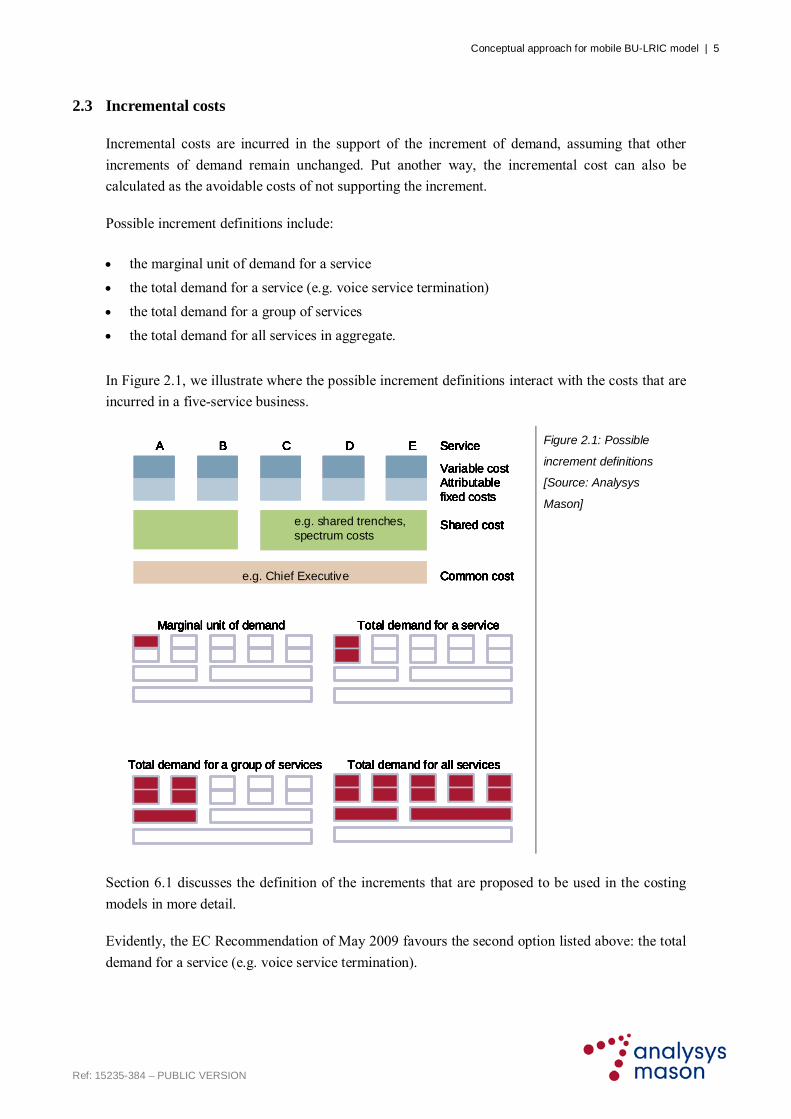
2.3 Incremental costs
Incremental costs are incurred in the support of the increment of demand, assuming that other
increments of demand remain unchanged. Put another way, the incremental cost can also be
calculated as the avoidable costs of not supporting the increment.
Possible increment definitions include:
the marginal unit of demand for a service
the total demand for a service (e.g. voice service termination)
the total demand for a group of services
the total demand for all services in aggregate.
In Figure 2.1, we illustrate where the possible increment definitions interact with the costs that are
incurred in a five-service business.
A B C D E
e.g. Chief Executive
Variable costAttributable fixed costs
Shared cost
Common cost
Service
Marginal unit of demand Total demand for a service
Total demand for a group of services Total demand for all services
A B C D E
e.g. shared trenches, spectrum costs
e.g. Chief Executive
Shared cost
Common cost
Service
Marginal unit of demand Total demand for a service
Total demand for a group of services Total demand for all services
A B C D E
e.g. Chief Executive
Variable costAttributable fixed costs
Shared cost
Common cost
Service
Marginal unit of demand Total demand for a service
Total demand for a group of services Total demand for all services
A B C D E
e.g. shared trenches, spectrum costs
e.g. Chief Executive
Shared cost
Common cost
ServiceA B C D E
e.g. Chief Executive
Variable costAttributable fixed costs
Shared cost
Common cost
Service
Marginal unit of demand Total demand for a service
Total demand for a group of services Total demand for all services
A B C D E
e.g. shared trenches, spectrum costs
e.g. Chief Executive
Shared cost
Common cost
Service
Marginal unit of demand Total demand for a service
Total demand for a group of services Total demand for all services
A B C D E
e.g. Chief Executive
Variable costAttributable fixed costs
Shared cost
Common cost
Service
Marginal unit of demand Total demand for a service
Total demand for a group of services Total demand for all services
A B C D E
e.g. shared trenches, spectrum costs
e.g. Chief Executive
Shared cost
Common cost
Service
Marginal unit of demand Total demand for a service
Total demand for a group of services Total demand for all services
Figure 2.1: Possible
increment definitions
[Source: Analysys
Mason]
Section 6.1 discusses the definition of the increments that are proposed to be used in the costing
models in more detail.
Evidently, the EC Recommendation of May 2009 favours the second option listed above: the total
demand for a service (e.g. voice service termination).

Conceptual approach for mobile BU-LRIC model | 6
Ref: 15235-384 – PUBLIC VERSION
2.4 Efficiently incurred costs
In order to set the correct investment and operational incentives for regulated operators, it is
necessary to allow only efficiently incurred expenditures in cost-based regulated prices. In
practice, the specific application of this principle to a set of cost models depends significantly on a
range of aspects:
detail and comparability of information provided by individual operators
detail of modelling performed
the ability to uniquely identify inefficient expenditures
the stringency in the benchmark of efficiency which is being applied3
whether efficiency can be distinguished from below-standard quality.4
The Portuguese operators seem generally active in competitive retail markets, which include both the
competitive supply of services to end users, and the competitive supply of infrastructure and services to
those operators. Therefore, the a priori expectation of inefficiencies in the market may be limited.
However, it is still necessary to ensure that there is a robust assessment of efficiently incurred costs.
2.5 Costs of supply using modern technology
In a market, a new entrant that competes for the supply of a service would deploy modern
technology to meet its needs – since this should be the efficient network choice. This implies four
‘modern’ aspects: (i) the choice of network technology (e.g. 2G, 3G); (ii) the capacity of the
equipment; (iii) the price of purchasing that capacity, and the costs of operating; and (iv) the cost of
maintaining the equipment. Therefore, a LRIC model should be capable of capturing these aspects:
The choice of technology should be efficient – Legacy technologies, which are in the process
of being phased out, should not be considered modern.
Equipment capacity should reflect the modern standard – In the case of mobile network
infrastructure, some network elements are functionally required to have a fixed capacity (e.g. a
global system for mobile communications (GSM) transceiver – or TRX – has a capacity of
eight channels), whereas other network elements have capacity that increases with new
hardware versions and technology generations (e.g. mobile switching centre–MSC processor
capacity), but decreases with the loading of new features5 – some of which will be deployed
for non-voice services. New-generation switches may also be optimised to give improved
capacity (e.g. the mobile network mobile switching centre server (MSS) only performs
3 For example, most efficient in Portugal, most efficient in Europe, most efficient in the world.
4 For example, an operator may appear to be carrying the annual traffic in its network with a relatively low deployment of capacity.
However, it may be achieving this with a higher busy-hour blocking probability (e.g. 5%), whereas the ‘efficient’ benchmark adopted
could be 2% (or other figure as specified in an operator’s licence conditions).
5 Much like the power and features of Microsoft Windows PCs over time.

Conceptual approach for mobile BU-LRIC model | 7
Ref: 15235-384 – PUBLIC VERSION
control-plane switching, whilst the separate media gateway (MGW) switches the user-plane
voice traffic). New-generation switches may not be simply dedicated to 2G or 3G but switch
both 2G and 3G traffic (e.g. using all IP core).
The modern price for equipment represents the price at which the modern asset can be
purchased over time. It should represent the outcome of a reasonably competitive tender for a
typical supply contract in Portugal. It is expected that operators in Portugal should be able to
acquire their equipment at typical European prices given that they are part of large
international groups with centralised sourcing, or they should have a comparable purchasing
power to that of their European peers. A data request has been sent to the Portuguese mobile
operators in order to obtain their estimate of the unit costs for the different network elements.
We expect to complement the Portuguese data points with European benchmarks in order to
come to a final view of the equipment costs in the model.
Operation and maintenance costs should correspond to the modern standard of equipment, and
represent all the various facility, hardware and software maintenance costs relevant to the
efficient operation of a modern standard network.
The definition of modern equipment is a complex issue. Mobile operators around the world are at
different stages of deploying IP-based core networks, from initial plans to fully deployed, as well
as at different stages of 3G upgrade: including radio layer augmentation for voice, high-speed
downlink packet access (HSDPA) and high-speed uplink packet access (HSUPA), and the extent
to which MSS/MGW switching has been rolled out.
The May 2009 Recommendation states that, in principle, the efficient technological choice upon
which the cost models for mobile operations should be based are:
a next-generation based core network
a combination of 2G and 3G employed in a radio mobile network.
These appear to be the current efficient technologies applicable to Portugal; the technology
architecture is discussed in Section 4.1.

Conceptual approach for mobile BU-LRIC model | 8
Ref: 15235-384 – PUBLIC VERSION
3 Operator issues
This section discusses the following aspects of the modelled operator:
type of operator (Section 3.1)
network footprint of the operator (Section 3.2)
scale of the operator (Section 3.3).
3.1 Type of operator
The type of operator to be modelled is the primary conceptual issue, which determines the
subsequent structure and parameters of the model. This conceptual issue is also important because
of the need to be able to ensure consistency between the choice of operator in the mobile
termination model and subsequent cost-based regulation of real players.
The full range of operator choices is:
Actual operators – in which the costs of all actual market players are calculated.
Average operator – in which the players are averaged together to define a ‘typical’ operator.
Hypothetical new entrant – in which a hypothetical new entrant to the market is defined as
an operator entering in 2011 with today’s modern network architecture, which acquires a
specified target share of the market.
Hypothetical existing operator – in which a hypothetical existing operator in 2011 is
modelled as an existing operator launching services in the Portuguese market in 2006 after
having rolled out a network in 2005 (the approximate date at which today’s modern
technology was deployed) with a modern network architecture, allowing the operator to attain
its hypothetical scale around the relevant period of regulation.
At this stage, we exclude the option to apply actual operators. This is because:
It would reduce costing and pricing transparency, as well as increasing the risk/complexity of
ensuring that identical principles are applied to individual operator models for all three mobile
players.
The EC recommends costing an operator with a minimum efficient scale of 20% – by
implication, not an actual operator. In the case of Portugal, this would entail a possible range
of market share between 20% (the EC minimum) and 33% (the equal market share for three
network operators).

Conceptual approach for mobile BU-LRIC model | 9
Ref: 15235-384 – PUBLIC VERSION
Therefore, we consider three options for the type of operator to be modelled. The characteristics of
these options are outlined below in Figure 3.1.
Characteristic Option 1: Average
operator
Option 2: Hypothetical
existing operator
Option 3: Hypothetical
new entrant
Date of entry Different for all operators, therefore an average date of entry is not meaningful
Can be set to take into account key milestones in the real networks (e.g. beginning of the phasing of 2G to 3G)
In this case, the date of entry is inferred from the EC Recommendation, which sets a relation between time and the acquisition of market share
Technology Different for all mobile operators (e.g. level of roll-out of all IP core), therefore an average mobile is not appropriate, most advanced operators would bear the costs of less-efficient ones (see ‘efficiency’ section below)
The technology of a hypothetical operator can be specifically defined, taking into account relevant recent technology components of existing networks. In the case where the hypothetical existing operator is modelled as an operator entering the market in recent years, the EC Recommendation specifies the appropriate technology mix
By definition, a hypothetical new entrant would employ today’s modern technology choice. The EC specifies a next-generation network (NGN) mobile core and a mix of 2G and 3G radio technology. Long Term Evolution (LTE) is not a technology available for a new entrant to deploy now in Portugal
Evolution and migration to modern technology
All mobile operators are currently using modern technology (combined GSM and UMTS networks) but are at different roll-out stages for their core network
The evolution and migration of a hypothetical operator can be specifically defined, taking into account the existing networks. Legacy network deployments can be ignored if migration to next-generation technology is expected in the short-to-medium term or has already been observed in real networks
By definition, a hypothetical new entrant would start with the modern technology. Therefore, evolutionary or migratory aspects are not relevant. However, the rate of network roll-out and subscriber evolution will be key inputs into the model
Efficiency May include inefficient costs through the average
Efficient aspects can be defined. If modelled as a new operator entering the market in recent years, efficient choices can be made throughout the model
By definition, efficient choices can be made throughout the model
Comparability and transparency of bottom-up network modelling with real operators
The network model of an average operator would only be comparable with an average across the real network operators. However, it would be possible to illustrate this average comparison in a reasonably transparent way
In order to compare a hypothetical operator network model with real operators, it would be necessary to transform the actual operator information in some way (e.g. averaging, or re-scaling to reflect the characteristics of the hypothetical operator). Whilst the hypothetical operator model would be transparent to industry parties, the comparison against real operator information might include additional steps which need to be explained
In principle, the hypothetical new entrant approach is fully transparent in design. However, since none of the real operators is a new entrant, it would not be possible to do a like-for-like comparison against real operator network information

Conceptual approach for mobile BU-LRIC model | 10
Ref: 15235-384 – PUBLIC VERSION
Characteristic Option 1: Average
operator
Option 2: Hypothetical
existing operator
Option 3: Hypothetical
new entrant
Practicality of reconciliation with top-down accounting data
It is not possible to directly compare an average operator with actual top-down accounts. Only indirect comparison (e.g. overall expenditure levels and operational expenditure (opex) mark-ups) is possible
It is not possible to directly compare a hypothetical existing operator with actual top-down accounts. Only an indirect comparison (e.g. overall expenditure levels and opex mark-ups) is possible
It is not possible to directly or indirectly compare a hypothetical new entrant model to real top-down accounts without additional transformations in the top-down domain (e.g. current cost revaluation). No new-entrant accounts exist
Figure 3.1: Operator choices [Source: Analysys Mason]
There are four key issues in resolving this choice:
Is the choice
appropriate for
setting cost-based
regulation?
All three options presented above could be considered a reasonable basis
on which to set cost-based regulation of wholesale mobile termination
services. However, in the case of Option 1, inefficient costs would need to
be excluded.
What modifications
and transformations
are necessary to
adapt real
information to the
modelled case?
Figure 3.1 above summarises the various transformations, which will be
required in the modelling approach. As an example of one of the main
transformations (date of entry), Figure 3.2 below illustrates the diversity in
dates of entry in terms of the technology layers in the networks. In all three
choices of operator outlined above, a GSM date of entry transformation is
required.
1992 1994 1996 1998 2000 2002 2004 2006 2008 2010 2012 2014 2016
2G, 2.5G (GSM, EDGE)
3G (WCDMA)
3.5G (HSPA)
Aug 98Jun 04
Sep 06
Oct 92Apr 04
Apr 06
Oct 92Jan 04
Apr 06
OPTIMUS
TMN
VODAFONE
4G (LTE)
?
?
?
National
National
National
Nearly-national
Nearly-national
Nearly-national
Sub-national
Sub-national
Sub-national
Not deployed
Not deployed
Not deployed
Figure 3.2: Timeline comparison for the Portuguese mobile operators [Source: Analysys Mason]

Conceptual approach for mobile BU-LRIC model | 11
Ref: 15235-384 – PUBLIC VERSION
Are there guidelines
which should be
accommodated?
(e.g. EC
Recommendation)
The EC Recommendation suggests that an efficient-scale operator should
be modelled; however, the precise characteristics of this type of operator
are not defined (other than its minimum scale). In principle, all three of the
above options can satisfy the efficient-scale requirement.
Flexibility A model constructed for Option 3 would be designed in such a way as to
exclude historical technology migrations. It would also be mechanically
designed to start its costing calculations in 2011. Therefore, the model for
Option 3 can be considered linked to the type of operator modelled.
A model constructed for Option 2 can, if known at the outset, also be used
to calculate costs for Option 3 by assuming a MEA deployment from the
beginning of the period of operation and adjusting the subscriber demand
and take-up.
Proposed Concept 1: We do not recommend Option 1 (average operators) as it is
dominated by historical issues rather than modern and efficient network aspects.
We propose that the cost model be based on Option 2 (hypothetical existing operator)
since this enables the model to determine a cost consistent with the existing suppliers of
mobile termination in Portugal, such that actual network characteristics over recent time
can be taken into account.
However, we consider that such a hypothetical existing operator could be modelled by an
operator starting services four years before today (2011), rolling out services a year
before launching services. Reflecting the May 2009 Recommendation, such an operator
network would use the technology that an efficient operator at the time of entry would
have rolled out, in anticipation of the situation for the years to come, i.e. a combination
of 2G and 3G network and an NGN core.
The operator modelled would therefore be:
A mobile operator rolling out a national 900MHz 2G network in 2005, launching 2G
services in approximately 2006, and supplementing its 900MHz network with extra 2G
capacity in the 1800MHz frequency band when necessary. This network would also be
overlaid with 2100MHz 3G voice and HSPA capacity and switch upgrades (reflecting
the technology available in the period 2005–2011), to carry increased voice traffic,
mobile data and mobile broadband traffic. The parallel 2G and 3G networks would be
operated for the long term, and thus complete migration off the modern 2G to the 3G
network would not be modelled. This is consistent with our discussions with operators,
which indicate that there is no expectation they will switch off the 2G network in the
foreseeable future.

Conceptual approach for mobile BU-LRIC model | 12
Ref: 15235-384 – PUBLIC VERSION
Industry comments
Four parties agree with the proposal to base the mobile model on Option 2 (hypothetical existing
operator).
One of them raises a set of questions and indicates that it needs to know the details associated with
the practical implementation of the hypothetical existing operator before validating its choice:
How can a model based on this operator be compatible with a top-down reconciliation of the
model?
The definition of the type of operator cannot be done as a theoretical-only exercise, and needs
to consider all its practical implications
This decision has many associated variables, such as market share and amount of years to
attain scale, traffic profile (volume and composition), infrastructures, etc.
There is a lack of information on the dimension of the progressive migration between 2G and
3G, nor other technologies that operators will have to implement such as LTE.
Another operator believes the definition of a 2G and 3G operator is incompatible when
considering a 45 year model, a period of time that will likely see different technological evolutions
that will lower the costs of voice traffic. It believes that a shorter time frame should be considered
to keep the existing 2G and 3G technological base, or alternatively 4G technologies should be
considered with a longer time frame.
Two parties disagree with using a hypothetical existing operator.
One of them disagrees because it argues that results are sensitive to the choice of when it is
assumed that the network started to be rolled out and when service began, that there may be
legacy effects and redundant assets as a result of the transition from one technology to another,
that it is not consistent with a contestable market, and that the output profile assumed prior to
2011 – given the use of economic depreciation – has a substantial impact on depreciation from
2011 onwards. It believes that it would be better to base the model on a hypothetical new
entrant that operates at full scale from the moment it comes into the market – and submit that
other regulators have accepted a hypothetical entrant operator as valid.
One of them disagrees because it believes that it is unrealistic to expect a new entrant to
achieve 20% market share in the period 2006/7 – 2011. They also argue that it is unrealistic to
expect an operator to survive in the market for a long time with a given set of technologies (2G
and 3G) without doing the effort of updating their network, as network-related decisions
cannot be taken independently and are linked to past deployments and decisions.
According to this operator, a hypothetical existing operator would not reflect the efficient
reality confronted by operators, which have to maximize the performance of their past
investments with the deployment of more modern technologies. The operator also highlights
the importance of reconciling the BU model with operator data, specifically for a first version
of the model.

Conceptual approach for mobile BU-LRIC model | 13
Ref: 15235-384 – PUBLIC VERSION
Analysys Mason response
Although numerous parties agreed with the proposed concept, some parties have indicated that
they prefer a hypothetical new entrant model. [Begin confidential (BC)]
[End confidential (EC)]
One party indicates that results are sensitive to the choice of the starting date for network roll-out
as there may be legacy effects and redundant assets as a result of the transition from one
technology to another. Actual operators are generally undergoing steady (manageably predictable)
evolutions: entire network redundancy has not occurred in a short-term period, whereas various
parts of the network have been individually replaced with newer technologies and generations over
time. However, because we envisage continued usage of 2G networks in the coming years, we do
not anticipate a major 2G asset redundancy. The modelled operator will start deploying its network
in 2005 with the latest technology and will not experience any technology transition as state-of-
the-art technologies are deployed from the outset. However the modelled operator will deploy an
entire new network rather than the ongoing replacements that actual operators experience. Given
the modelling of an entire new network, we do not consider it reasonable to also include short-term
asset redundancy effects.
One party mentioned that a hypothetical existing operator would not reflect the efficient reality
faced by operators. We believe that paragraph 12 of the EC Recommendation is consistent with
our proposed methodology, reflecting the level of costs for an operator characterised by reasonably
efficient modern technology choices – not necessarily the most efficient possible technology
choices which might be taken in a 2011 greenfield situation. As the EC Recommendation notes, it
is necessary to be able to identify the relevant technology choices and we consider it reasonable at
this point to refer to actual operators’ recent activities, and to capture these in an existing operator
model.
We do not model an LTE operator, as market entry using this particular technology is not required
of any market players – it is within the control of market parties and is not an uncontrollable
exogenous factor. Therefore the fact that LTE costs might be different than those of the modelled
GSM+UMTS operator is not directly relevant. For example, because it may initially only be
available in high-frequency (2600MHz) bands, and because there are currently no existing
Portuguese LTE operators on which to validate such a bottom-up cost calculation, it is not clear
how accurate LTE costs could be ensured (and compared with 2G+3G costs). Furthermore, it is
unlikely that any significant volumes of voice (termination) traffic will migrate off 2G and 3G and
onto LTE within the next three years.
One of the parties queries how a model based on a hypothetical operator can be compatible with a
top-down reconciliation, claiming an accurate reconciliation process would have required
modelling an existing operator’s network and costs and comparing the model outputs to ensure
both are within a reasonable margin of error. We are considering a hypothetical operator, which

Conceptual approach for mobile BU-LRIC model | 14
Ref: 15235-384 – PUBLIC VERSION
gives rise to the concept of calibration. During the calibration process, we will use input data
provided by existing operators – such as coverage, demand, unit costs – in the model and compare
the outputs with the total costs of existing operators, aiming at validating the costs for each
operator and in aggregate for the market. We will focus our calibration efforts on ensuring that the
total number of sites, BTS, and NodeBs produced by the model is compatible with the market
numbers as an aggregate. We will also calibrate the cost base in aggregate for the market, by
referring to submitted operator information on total expenditures and book-values.
Some respondents have commented on issues regarding details of the operator modelled. We will
be commenting on these in the corresponding sections:
we comment on market share achieved by the operator and rate at which it achieves it in
Concepts 3 and 4
we comment on the technologies (2G/3G) modelled and on the use of efficient modern
technology in Concept 5, 7 and 8
we comment on the 2G/3G migration issue in the Concept 13
we comment on the issue of the model period of time in the Proposed Concept 17.
Conclusions
Concept 1: The cost model will be based on Option 2 (hypothetical existing operator) since
this enables the model to determine a cost consistent with the existing suppliers of mobile
termination in Portugal, such that actual network characteristics over time can be taken into
account.
To ensure that the hypothetical existing operator reflects the reality of the Portuguese market,
the model will be calibrated against network and financial data provided by the three mobile
operators. We will focus our calibration efforts on ensuring that the total number of sites, BTS,
and NodeBs produced by the model is consistent with the market numbers as an aggregate. We
will also calibrate the cost base in aggregate for the market, by referring to total expenditures
and book-values.
3.2 Network footprint of operator
Coverage is a central aspect of network deployment. The question of what coverage to apply to the
modelled operator can be understood as follows:
What is the current level of coverage applicable to the market today?
Is the future level of coverage different from today’s level?
Over how many years does the coverage roll-out take place?
What quality of coverage should be provided, at each point in time?
The coverage offered by a mobile operator is a key input to the costing model. The definitions of
coverage parameters have two important implications for the cost calculation:

Conceptual approach for mobile BU-LRIC model | 15
Ref: 15235-384 – PUBLIC VERSION
The unit cost of
traffic is affected by
the expenditure of
coverage roll-out
The rate, extent and quality of coverage achieved determine the network
investments and operating costs of the coverage network in the early years.
The degree to which these costs are incurred prior to demand materialising
represents the size of the ‘cost overhang’. The larger this overhang, the
higher the eventual unit costs of traffic will be. The concept of a cost
overhang is illustrated in Figure 3.3.
Time
Demand
Coverage
cost overhang as coverage precedes demand
Time
Demand
Coverage
cost overhang as coverage precedes demand
Figure 3.3: Cost
overhang [Source:
Analysys Mason]
Identification of
network elements
that vary in
response to traffic
Elements of the mobile networks may (or may not) vary in response to the
carried traffic volumes – depending on whether the coverage network has
sufficient accompanying traffic capacity for the offered load. This has
particular implications during the application of a small wholesale
termination traffic increment (see Section 6.1 on Choice of Increment).

Conceptual approach for mobile BU-LRIC model | 16
Ref: 15235-384 – PUBLIC VERSION
Approach
All mobile networks in Portugal currently have almost ubiquitous 2G and 3G outdoor population
coverage. As all mobile networks have practically ubiquitous outdoor coverage, this should be
reflected in the model.
Due to building penetration losses, good outdoor coverage does not directly translate into good
indoor coverage, and therefore deep indoor mobile coverage entails additional radio site
investments. This indoor coverage is delivered by either:
deploying outdoor macro site networks to transmit signals through the walls of buildings
installing a dedicated indoor picocell which is typically backhauled to the mobile switch via a
fixed link to the building. Indoor picocells may be classified as either public access (e.g. in
shopping centres) or private access (as in corporate in-building solutions).
These wireless solutions serve traffic, which might otherwise be carried to that building by a fixed access method with a dedicated or very high-capacity technology (or low marginal cost, in other words). It is estimated that up to 60% of mobile voice traffic occurs inside buildings; at least 30% from home or work.6
Because of current end-user expectations, and for the model to reflect current deployment practice and traffic volumes, we recommend including the current level of indoor coverage within the mobile network footprint principle.
Proposed Concept 2: National levels of geographical coverage will be reflected in the models: >99% of population in 2G and >80% of population for 3G, comparable to that offered by current mobile operators in Portugal, including indoor mobile coverage. To develop our coverage model,7 we will use internal estimates and/or calibration of macro- and micro-sites (and/or pico/indoor sites) with operator data8 if submitted.
Industry comments
Three parties agree with the presented levels of geographical coverage.
One of them points out that the EC explains that the model must take into account the necessity of
showing the costs of an efficient operator, and not do a reconciliation merely to bring the results of
6 Source: Strategy Analytics estimates ‘indoor’ as 57% of mobile usage; Korea Telecom estimates that 30% of calls were from home
or work (Source: Wireless Broadband Analyst, 14 November 2005); Swisscom estimates that 36% of usage is at home and 24% in
the office (Source: Swisscom Innovations paper, 2004).
7 Further details of the coverage and capacity calculation are provided in Annex A.
8 Once the coverage calculation is developed in the model, and loaded up with network traffic, we will be able to compare the modelled
numbers of BTS/Node Bs and TRXs/CE against actual operator data (if submitted). If this comparison process identifies significant differences
between the model and reality, further investigation will be required in order to validate the calculation model (e.g. investigating uncertain
model inputs, analysing operator data and differences, identifying relevant benchmarks from other European countries for comparison, or
adapting model inputs where appropriate).

Conceptual approach for mobile BU-LRIC model | 17
Ref: 15235-384 – PUBLIC VERSION
both models closer. The model should then take into account factors that might result in the
hypothetical efficient operator having lower costs than existing operators, such as:
having a coverage and network equipment deployment using the new technologies and/or
taking into advantage of spectrum liberalization, such as UMTS in the 900MHz bands
having a higher level of sharing of passive network elements between the hypothetical
efficient operator and existing operators compared to the level of site sharing between existing
operators.
Furthermore, it affirms that Optimus, TMN and Vodafone should have the opportunity to provide
information on the many other parameters necessary for LRIC modelling, and the opportunity to
question the proposed choices.
One party disagrees with the necessity to achieve a 3G coverage of 100% and submits that it could
entail inefficient costs either because of inefficient technology or because the existing equipment
could not use newer technologies or take advantage of existing spectrum (such as using the 900
MHz to deploy UMTS). It also submits it is necessary to consider in the modelling exercise the
passive network equipment present at the beginning of deployment, which will see the network
expanding in zones with less economic incentives that would, otherwise, remain without service.
Finally, another party understands that the coverage modelled should be proportional to those of
existing mobile operators, but warns over the fact that the Pure LRIC is sensitive to coverage
requirements, which does not appear to be recognized in the present document. Indeed, the long-
term objectives do not correspond to the reality of operators in the market. Any infrastructure
deployment must aim to balance coverage and capacity, and a network deployed for coverage only
would be very different from existing networks.
It proposes to consider the minimum coverage as based on the minimum traffic volume in the long
term. This would be, in its opinion, similar to the minimum network required to make a single call
in the coverage area of the hypothetical operator. The coverage should take into account the
information relative to the number of sites initially deployed in their network. [BC]
[EC]
This same party believes that, due to its importance, the model should calculate the geographical
and population coverage as not being sensitive to traffic, to clearly define the real component of
fixed costs. In reality, the majority of its network coverage is sensitive to traffic, as the
dimensioning of infrastructure is dependent of traffic. It also submits that the existence of a fixed
coverage cost does not imply that this cost should be completely excluded from incremental cost
of capacity. Indeed, it submits that Ofcom found in a study that only 3.3% of costs of a GSM900
network conceived to support traffic in 2005/6 could be related to coverage.
Analysys Mason response

Conceptual approach for mobile BU-LRIC model | 18
Ref: 15235-384 – PUBLIC VERSION
The differences between the network deployment of a hypothetical efficient operator and existing
mobile operators will be examined during the calibration process. As indicated in Concept 1 in this
document, we will calibrate our model with data from existing operators.
As part of the model build-up process a data request was sent to the mobile operators. Additionally
we held some meetings to clarify pending questions and give the operators the opportunity to
comment on model choices and the details of many other parameters necessary for LRIC
modelling.
In the context of the Consultation process and setting of termination prices, operators will have
access to the details of many other parameters used for the dimensioning of the network and
definition of the traffic shape in the terms made explicit by the Portuguese regulation in this
respect.
A party states that it does not understand why 3G coverage was projected to reach 100% of
population. As stated in the proposed concept, 3G coverage will be consistent with current
deployments and coverage commitments as set out in the operators’ respective 3G licenses. We
expect this coverage to reach 91% of population in the 2.1GHz band in 2021, which has been
extrapolated from existing coverage and coverage obligations for the three mobile operators.
Some parties mention the possibility that the new operator may take advantage of the recent
technology neutrality implementation in the 900MHz and 1800MHz spectrum band to deploy
UMTS or LTE in lower spectrum bands. Currently, there is an uncertainty associated with which
technologies and bands are more likely to be deployed in the future. Refarming spectrum involves
un-loading and re-configuring the spectrum usage to create empty (likely 2x5MHz) bands – which
appears to be a long-term rather than short-term challenge given the total amount of 900MHz
spectrum available to each operator. Refarmed spectrum is expected to be used above all to
provide data services to underserved areas, especially in the rural parts of the country. A relevant
issue will be the potential availability of UMTS900 handsets and their take-up among subscribers.
Operators are already experiencing some difficulties to increase 3G handset take-up as mentioned
in operator’s comments to Proposed Concept 13. Therefore we do not expect that significant
amounts of voice traffic will be carried on potentially refarmed spectrum during the next
regulatory review.
One party suggests that the model should include network sharing. Current levels of infrastructure
sharing have been explored in our data request and the outcome will be reflected in the model. We
will make a distinction between sites owned by the operators and sites rented from third parties.
Based on operators’ data, we believe the majority of sites in the Portuguese market are owned by
third parties and rented by operators. As far as we know, no new major infrastructure and RAN
sharing projects have been announced in Portugal for 2G and 3G infrastructure. We further
comment on network sharing in Concept 9.
Some parties appear to be concerned about the definition and implementation of coverage and
capacity. Pure LRIC is calculated as the difference between the network costs of an operator with
Conceptual approach for mobile BU-LRIC model | 19
Ref: 15235-384 – PUBLIC VERSION
all traffic included and the network costs of an operator with all traffic excluding termination
traffic. We thus recognise that pure LRIC is sensitive to the definition of coverage, and will
develop an appropriate model to ensure that results are consistent with the reality of the Portuguese
market.
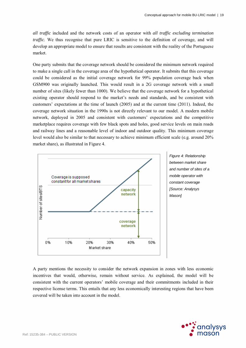
One party submits that the coverage network should be considered the minimum network required
to make a single call in the coverage area of the hypothetical operator. It submits that this coverage
could be considered as the initial coverage network for 99% population coverage back when
GSM900 was originally launched. This would result in a 2G coverage network with a small
number of sites (likely fewer than 1000). We believe that the coverage network for a hypothetical
existing operator should respond to the market’s needs and standards, and be consistent with
customers’ expectations at the time of launch (2005) and at the current time (2011). Indeed, the
coverage network situation in the 1990s is not directly relevant to our model. A modern mobile
network, deployed in 2005 and consistent with customers’ expectations and the competitive
marketplace requires coverage with few black spots and holes, good service levels on main roads
and railway lines and a reasonable level of indoor and outdoor quality. This minimum coverage
level would also be similar to that necessary to achieve minimum efficient scale (e.g. around 20%
market share), as illustrated in Figure 4.
Figure 4: Relationship
between market share
and number of sites of a
mobile operator with
constant coverage
[Source: Analysys
Mason]
A party mentions the necessity to consider the network expansion in zones with less economic
incentives that would, otherwise, remain without service. As explained, the model will be
consistent with the current operators’ mobile coverage and their commitments included in their
respective license terms. This entails that any less economically interesting regions that have been
covered will be taken into account in the model.

Conceptual approach for mobile BU-LRIC model | 20
Ref: 15235-384 – PUBLIC VERSION
One party believes that the model should calculate the geographical and population coverage as
being sensitive to traffic. We refer to the definition stated by the EC in its Recommendation, that
“the need to provide such coverage to subscribers will cause non-traffic-related costs to be
incurred which should not be attributed to the wholesale call termination increment”. In our model,
the coverage network will be deployed based on a specific rate of deployment and independent of
traffic, and a capacity network will be deployed where the coverage network cannot cope with the
voice and data traffic in each geotype.
Conclusions
Concept 2: National levels of geographical coverage and coverage regulatory obligations will
be reflected in the models. We expect outdoor coverage to be 99% of population in 2G and
91% of population for 3G. Indoor coverage is modelled based on the deployment of
micro/pico/indoor sites by operators. The model will classify Portuguese freguesias into
geotypes based on their average densities. We understand the sensitivity of the pure LRIC
methodology, and will adopt a definition of coverage consistent with the expectations of the
Portuguese market during the period of rollout (2005 to 2011).
3.3 Scale of operator
One of the main parameters that defines the cost (per unit) of the modelled operator is its market share: it is therefore important to determine the market share of the operator and the period over which any market share evolution/growth takes place.
The parameters chosen for defining the operator’s market share over time influence the overall
level of economic costs calculated by the model. The quicker the operator grows, the lower the
eventual unit cost of traffic should be.
Regarding the scale of the modelled operator, a minimum value of 20% is indicated by the May
2009 Recommendation9 for the efficient scale of an operator. This minimum efficient scale may be
considered consistent with the case of Portugal.
A further issue related to the issue of scale is the time taken to achieve a steady market share. It is
necessary to specify in the model the rate at which the modern network is rolled out, and the
corresponding rate at which that modern network carries the volumes of the operator (up to the
market share proposed above). There are a number of options in terms of modelling a hypothetical
existing operator:
9 EC Recommendation on the Regulatory Treatment of Fixed and Mobile Termination rates in the EU (2009/396/EC): To determine
the minimum efficient scale for the purposes of the cost model, and taking account of market share developments in a number of EU
Member States, the recommended approach is to set that scale at 20% market share. It may be expected that mobile operators,
having entered the market, would strive to maximise efficiency and revenues and thus be in a position to achieve a minimum market
share of 20%. In case an NRA can prove that the market conditions in the territory of that Member State would imply a different
minimum efficient scale, it could deviate from the recommended approach.
Conceptual approach for mobile BU-LRIC model | 21
Ref: 15235-384 – PUBLIC VERSION
Option 1: Immediate scale – In this option, the modelled operator immediately achieves its
market share, and rolls out its network just in time to serve this demand at launch. This
approach does not reflect real technology transitions.
Option 2: Matching the modern technology transition during the modelled years – In this
approach, the utilisation of the modern technology during the specific recent years is observed for
the actual networks and used to define an efficient profile for the hypothetical existing operator. In
this approach, we observe that mobile networks have not experienced any significant radio
technology transition between technology generations in the period 2005–2009, with 3G overlays
steadily carrying additional traffic.
Option 3: Assuming a hypothetical roll-out and market share profile – In this option, a time
period to achieve a target network coverage (footprint) roll-out would be specified (e.g. four years)
and a time-period to achieve full scale (e.g. 20%) would also be specified (e.g. four to five years).
Option 4: Roll-out and growth based on history – It is possible to apply roll-out and volume
growth profiles which have been obtained directly from (the average of) the actual mobile
operators. This approach would require looking back at networks a long time ago to the early
1990s, and therefore would be complex to carry out, with numerous assumptions based on
historical information.
Proposed Concept 3: We suggest a long-run market share of 20% for the hypothetical
existing operator, in line with the EC Recommendation for the minimum market share and
compatible with the evolution of the Portuguese market. In order to apply a minimum
efficient scale of 20%, we shall also need to specify minimum efficient levels of coverage,
quality and other deployment aspects (otherwise the modelled operator may be inefficient at
20% market share).
Proposed Concept 4: We suggest to consider Option 3, i.e. a time period to achieve a
target network coverage (footprint) roll-out of three to four years and a time-period to
achieve full scale (20%) of four to five years. Coverage deployments are, in many cases,
conditioned by i) spectrum licences, which often set coverage obligations for the operators
to which the licences are awarded, and ii) by the strategic choice of the operator in order to
compete and achieve a minimum market share. This is in line with the EC
Recommendation,10 which states that an operator is expected to take three to four years
after entry to reach a market share approaching the minimum efficient scale (15–20%). This
period of four to five years is also the approximate duration it has taken recent 3G networks
to reach near national coverage.
Industry comments on market share
Four parties agree with a long-run market share of 20%. [BC]
10 L124/69 Official Journal of the European Union (20 September 2009), paragraph 17.

Conceptual approach for mobile BU-LRIC model | 22
Ref: 15235-384 – PUBLIC VERSION
[EC] Another party indicates that, nonetheless, the termination traffic of such an operator would
represent a far higher proportion that the termination traffic of an operator with a higher market
share.
One party does not believe that 20% is the right benchmark to use in Portugal and propose a
modelled operator with market share of 100%/nb of mobile operators, which would correspond for
Portugal to 33.3%. It finds unclear why the operator’s market share should stagnate at this level
and stop growing, when an efficient operator, unencumbered by legacy costs, would be in a good
position to continue to capture market share. It believes that it is not obvious why the minimum
efficient scale (MES) should be the same across all European countries, and point out that it is
likely to change with various factors such as number of mobile subscribers, topography, level of
urbanization, etc. It also points out that the overstatement of unit costs from understating the MES
will be much higher than the understatement of unit costs from overstating the MES.
A party indicates that the EC Recommendation is not prescriptive concerning a market share of
20%, but indicates that a market share of between 15-20% enables approximating (but not
matching) a minimum efficient scale that would justify the transition period that, in terms of costs,
is appropriate for the existence of asymmetric regulation of termination taxes. On the other hand, it
argues that the Recommendation states a recommended scale of 1/number of operators.
Three parties believe that the determination of 20% market share would benefit of further analysis,
and that ANACOM should decide if the defined scale and hypothesis are applicable to the
Portuguese market.
Industry comments on time to achieve market share
Two parties agree with the defined timing to achieve the minimum efficient market share.
Four parties think that a roll-out of three to four years and a time-period to achieve full scale of
four to five years is not compatible with a contestable market with such high mobile penetration as
the Portuguese market. One party proposes to attain a 20% market share between 2000/1 and 2011.
Analysys Mason response on market share
One party believe that 20% is not the right benchmark for long-term market share, while one party
indicates that the EC is not prescriptive concerning the 20% market share. Their comments suggest
that the market share should be larger than 20%, or that the operator should grow past 20% with
MVNOs, or that the market share should be 1/number of operators – 33.3% for the Portuguese
market. Furthermore, a party notes that an efficient operator could continue to grow and gain
market share against its competitors past its minimum efficient scale.
We believe that an operator achieving a minimum efficient scale of 20% fits with the history of the
Portuguese market (with one operator at smaller scale) and fits with the EC Recommendation for
the initial years of the modelled operator deployment. We also agree with the argument of the

Conceptual approach for mobile BU-LRIC model | 23
Ref: 15235-384 – PUBLIC VERSION
suitability of a 33.3% market share in the long term, as it has been used by other regulators in
European countries where there is a three-player market situation; it is also consistent with a
competitive market of three operators. In order to respond to both concerns we will adapt the
market share profile so that it reaches 20% at the beginning of the period considered for setting
wholesale termination prices (2011), but attains a market share of 33.3% in the longer-term (in
2017).
Analysys Mason response on time to achieve market share
Some parties submit that a three- to four-year roll-out period, with full scale being achieved within
four to five years is not compatible with a contestable market with high mobile penetration, as seen
in the Portuguese market. As we are not modelling a new entrant operator, the rate of market
growth that a new entrant might achieve is not relevant. We believe that modelling an existing
player deploying a new network and loading it up over a relatively short period of time in a fully
penetrated market is consistent with the efficient termination cost constraint to be placed on
existing MNOs. We will model an operator that attains a minimum efficient scale of 20% in six
years, and grows to the proposed 33.3% in the long run.
Conclusions
Concept 3: We will model a hypothetical existing operator attaining a minimum efficient scale
of 20% in the short term, in line with the EC Recommendation for the minimum market share
and compatible with the evolution of the Portuguese market. We also propose that the
operator’s market share grows to 33.3% by 2017, reflecting the average market share of a
three-operator market.
Concept 4: We will model a time period to achieve network coverage similar to other
Portuguese mobile operators’ coverage (footprint) of six years. Coverage deployments are, in
many cases, conditioned by i) spectrum licences, which often set coverage obligations for the
operators to which the licences are awarded, and ii) by the strategic choice of the operator in
order to compete and achieve a minimum market share. This is in line with the EC
Recommendation, which states that an operator is expected to take three to four years after
entry to reach a market share approaching the minimum efficient scale (15–20%).

Conceptual approach for mobile BU-LRIC model | 24
Ref: 15235-384 – PUBLIC VERSION
4 Technology issues
This section describes the most important conceptual issues with regard to technology in mobile
BU-LRIC models. It is structured as follows:
choice of modern network architecture (Section 4.1)
treatment of network nodes (Section 4.2)
dimensioning of the network and impact of data traffic (Section 4.3).
4.1 Modern network architecture
The mobile BU-LRIC model will require a network architecture based on a specific choice of
modern technology. From the perspective of termination regulation, modern-equivalent
technologies should be reflected in the model: that is, proven and available technologies with the
lowest cost expected over their lifetimes.
Mobile networks have been characterised by successive generations of technology, with the two most
significant steps being the transition from analogue to 2G digital (GSM), and an ongoing expansion to
include UMTS (3G)-related network elements and services. The mobile network architecture splits into
three parts: a radio network, a switching network and a transmission network. Below we discuss the
(modern) technology generations to apply to the model.
Radio network generation and technology
Radio networks rely on spectrum bands to carry the traffic load. The Portuguese market enjoys
almost complete spectrum symmetry between its operators, resulting from how the spectrum
assignment process has been managed in the past:
GSM 900MHz spectrum bands were awarded to the Portuguese operators with a six-year
interval between the first and the last operator. Vodafone obtained a GSM licence in 1991;
TMN was assigned GSM frequencies in 1992; and Optimus obtained a GSM licence in 1997.
DCS 1800MHz spectrum bands were awarded in equal proportion to all three mobile operators
in the same year when Optimus entered the market (1997).
The UMTS 2100MHz spectrum bands were awarded in 2000. Four operators received a
licence: Vodafone, Optimus, Portugal Telecom and OniWay. However, OniWay’s licence was
revoked in 2003 due to the inability of the operator to deploy its network, and its 15MHz of
spectrum was distributed equally between the remaining three operators. Deployment
obligations were delayed until 2004 due to technological and economic reasons.

Conceptual approach for mobile BU-LRIC model | 25
Ref: 15235-384 – PUBLIC VERSION
There are, however, a few small asymmetries in the actual frequency assignment among
Portuguese operators:
in the GSM 900MHz spectrum band, Optimus has 39 2200KHz channels instead of the
40 channels that each of Vodafone and TMN has
in the UMTS 2100MHz band, Optimus returned its 5MHz of time division duplex (TDD)
spectrum in February 2009.
There are some aspects of spectrum allocations which have evolved over time, and are expected to
develop in the future:
technological restrictions were lifted from the use of 900/1800MHz band frequencies in
March 2010; these frequencies are now technology neutral
it could be that in the near future all spectrum rights may be unified into a single title plan,
with similar conditions for the rights of use in all frequency bands (GSM 900/1800MHz and
UMTS 2100MHz), for the provision of land mobile services.
Figure 4.1 provides details of the current spectrum allocation in Portugal for all mobile operators.
TMN Vodafone Optimus
GS
M 9
00M
Hz
Frequencies 40 channels (16MHz)(1) 40 channels (16MHz) (1) 39 channels (15.6MHz)
Assigned 16 March 1992 19 October 1991 20 November 1997
Renewed 16 March 2007 19 October 2006 N.A.*
Expiration 16 March 2022 19 October 2021 20 November 2012
Licence cost Financial allocations pending
Comments The licence was automatically granted
to TMN
10 additional channels were provided in 1996
10 additional channels were provided in 1996
Awarded jointly with 1800MHz licence
Award system Automatically granted Public tender Beauty contest
GS
M 1
800M
Hz
Frequencies 30 channels (12MHz) 30 channels (12MHz) 30 channels (12MHz)
Assigned 20 November 1997 20 November 1997 20 November 1997
Renewed 16 March 2007 19 October 2006 N.A.
Expiration 16 March 2022 19 October 2021 20 November 2012
Licence cost Financial allocations pending
Comments Awarded jointly with 1800MHz licence
Award system Automatically granted Automatically granted Beauty contest

Conceptual approach for mobile BU-LRIC model | 26
Ref: 15235-384 – PUBLIC VERSION
TMN Vodafone Optimus
TMN Vodafone Optimus
UM
TS
210
0MH
z
Frequencies 1920–1980/ 2110–2170MHz
220MHz paired spectrum
220MHz paired spectrum
220MHz paired spectrum
Frequencies 1900–1920MHz
5MHz unpaired spectrum 5MHz unpaired spectrum No spectrum
Assigned 11 January 2001 11 January 2001 11 January 2001
Expiration 11 January 2016 11 January 2016 11 January 2016
Licence cost PTE 20 billion per licence fee + annual spectrum fee
Comments Paired spectrum was increased from 215MHz
to 220MHz in December 2003
Paired spectrum was increased from 215MHz
to 220MHz in December 2003
Paired spectrum was increased from 215MHz
to 220MHz in December 2003
In February 2009, Optimus returned its 5MHz of unpaired
spectrum
Award system UMTS frequencies where awarded based on a beauty parade (public tender) (1)10 channels were provided in addition to the existing 30 channels in 1996.
Figure 4.1: Current situation of spectrum allocation in Portugal [Source: ANACOM, Analysys Mason]
*Note: N.A = Not available
Proposed Concept 5: Since all operators own similar 900MHz, 1800MHz and 2100MHz
spectrum allocations, it is assumed that forward-looking spectrum and coverage network-
related costs are symmetrical. We suggest to model an operator with:
28MHz of GSM 900MHz spectrum
26MHz of DCS 1800MHz spectrum
220MHz of UMTS 2100MHz spectrum.
It is likely that 3G networks in Portugal currently carry significant volumes of mobile broadband
(HSPA) traffic in their first and (more likely) second carriers. In the pure BU-LRIC approach, the
3G spectrum basic licence (2×20MHz) will not be considered sensitive to wholesale termination
traffic volumes in the long run.
Industry comments
Five parties agree in principle with the presented distribution of frequencies.
One party points out that in July 2010 technological restrictions on the use of 900Mhz and
1800MHz spectrum were lifted in Portugal, opening the door to spectrum refarming in those bands
for use with 3G, which is an efficient choice that the operator would make and should be included
in the model to build. The model should consider the possibility of refarming, likely allowing the
deployment of UMTS in the 900MHz band, which would result in lower unit costs.

Conceptual approach for mobile BU-LRIC model | 27
Ref: 15235-384 – PUBLIC VERSION
Another third party points out that the spectrum distribution suggested does not take into account
the future potential distribution of spectrum in the 450MHz, 800MHz, 900MHz, 1800MHz,
2.1GHz and 2.6GHz frequency bands.
Analysys Mason response
We comment on refarming in Proposed Concept 2.
One party submits that the spectrum distribution suggested does not take into account the outcome
of the upcoming auction. We believe that spectrum information available at the current time of
modelling should be used. We believe that the spectrum currently owned by mobile operators is
enough to carry the voice traffic they generate at present and within the model’s forecast. We also
note that all of the spectrum in the auction will be additional to that already held by the three
Portuguese MNOs, which indicates that the spectrum is unlikely to be considered for carrying
current levels of termination traffic. Therefore, we do not expect the coming auction to be relevant
for the modelling exercise being considered in this Concept Paper.
We discuss the issue of the potential incremental nature of some spectrum in Concept 6.
Conclusions
Concept 5: Since all operators own similar 900MHz, 1800MHz and 2100MHz spectrum
allocations, it is assumed that the spectrum allocations are symmetrical. We will model an
operator with:
2x8MHz of GSM 900MHz spectrum
2x6MHz of DCS 1800MHz spectrum
2x20MHz of UMTS 2100MHz spectrum.
Spectrum payments
The EC Recommendation states that only additional spectrum acquired to provide the wholesale
termination service should be taken into account.11 This is an extension of the EC’s principles that only
wholesale termination incremental costs should be taken into account and the exclusion of common
cost mark-ups. This means that, in many cases, the amounts paid for spectrum would need to be
excluded from any cost calculations. The majority of Portuguese up-front auction fees or beauty-
contest obligations will have been incurred as a common cost, and thus fall outside the EC proposition.
11
Extract from the EC Recommendation: The costs of spectrum usage (the authorisation to retain and use spectrum frequencies) incurred in
providing retail services to network subscribers are initially driven by the number of subscribers and thus are not traffic-driven and should not
be calculated as part of the wholesale call termination service increment. The costs of acquiring additional spectrum to increase capacity
(above the minimum necessary to provide retail services to subscribers) for the purposes of carrying additional traffic resulting from the
provision of a wholesale voice call termination service should be included on the basis of forward-looking opportunity costs, where possible.

Conceptual approach for mobile BU-LRIC model | 28
Ref: 15235-384 – PUBLIC VERSION
There are four possible approaches to estimating the cost of 900MHz, 1800MHz and 2100MHz
spectrum applicable to the model:
Option 1 – reflect the actual amounts paid by operators for spectrum.
Option 2 – reflect the cost of spectrum, which could realistically be paid, if historical reality
of spectrum payments had been different. This is mostly relevant in the cases where spectrum
assigned through auction mechanisms have raised significant amounts. In such a case, an
approach through benchmarking recent mobile frequency auctions could be used.
Option 3 – the cost of spectrum is estimated from other public sources and not from auctions,
for instance from published price lists obtained at national regulatory agencies for the cost of
spectrum.
Option 4 – value the spectrum using an independent forward-looking estimate.
In the case where spectrum costs are estimated from benchmarks of auction prices or from other
public sources, the information can be analysed according to three categories:
paired 900MHz frequencies, typically reflecting the provision of wide-area mobile coverage
paired 1800MHz frequencies for providing second-generation mobile capacity expansion
paired 2100MHz frequencies for providing a mobile broadband overlay network.
In Portugal, the price paid for spectrum is essentially achieved through annual spectrum payments
rather than through the one-off acquisition of a spectrum licence. Indeed, 3G spectrum in Portugal
has been acquired for a significantly lower price (in 2001) than in other European countries such
as France or the UK.
Proposed Concept 6: We propose to consider actual amounts paid by Portuguese operators
(Option 1) for the spectrum in Portugal that is considered to be incremental to wholesale
termination traffic in the BU-LRIC model. Given that the EC Recommendation states that
only additional spectrum acquired to provide the wholesale termination service should be
taken into account, 3G spectrum shall not be considered incremental in the pure LRIC
model. It will be analysed whether any 2G spectrum (and its associated cost under
Option 1) that was acquired to extend the capacity of the network is sensitive to wholesale
termination traffic, and its potential allocation to the wholesale termination service.
Industry comments
Three parties agree with the option considered.
One of them believes that it is incorrect to characterize the 2100MHz spectrum as being used
solely for mobile broadband (data) overlay, as it contradicts Proposed Concept 10 and does not
necessarily represent the efficient choice that the hypothetical operator would make. It also points
out that that Ofcom argues that although in theory a mobile operator with no terminating traffic

Conceptual approach for mobile BU-LRIC model | 29
Ref: 15235-384 – PUBLIC VERSION
might need to purchase less spectrum, a trade-off exists between spectrum use and network costs
such that in practice the Pure LRIC of termination is the same whether spectrum costs are included
or not. As a result Pure LRIC is the same whether or not spectrum is considered incremental to
termination.
Three parties do not agree with the proposed valuation of the spectrum.
Two of them suggest that the cost could be inferred using the coming spectrum auctions as proxies
for the estimation of the final price, re-using the resulting price per MHz.
One party believes that historic costs do not reflect correctly the value of spectrum, and that its
long-term cost should be incorporated. It also considers that the cost should include both the initial
payments and the yearly payments associated with the spectrum. It also would like to better
understand the allocation mechanisms of the spectrum cost to the products and services
considered.
Another party believes that the majority of spectrum varies with voice traffic, including
termination traffic, and concludes that ANACOM’s proposal will be valid only if they reflect the
economic value of the spectrum, in conformity with what is indicated in the EC Recommendation
over the future opportunity cost of spectrum.
Furthermore, it estimates that the spectrum mainly serves to increase capacity and that ownership
of spectrum is a trade-off between cost of spectrum and cost of additional deployments of sites.
Thus, the spectrum required for initial coverage is minimal, and significantly lower than the
spectrum currently allocated to operators. It believes that the cost of spectrum should be
considered incremental, as:
it can be negotiated or returned to the State, which implies the existence of an opportunity cost
in the long term for the ownership of the spectrum
it is a variable cost with traffic capacity beyond the minimum needed to provide the minimum
coverage.
This party states that a methodology to calculate the fixed and variable costs of spectrum is
required. For 2G it suggests the following:
2x2.4MHz in 900MHz band for coverage based on the minimum spectrum to convey a single
call
2x5.6MHz in 900MHz band and 2x6MHz in 1800MHz band for capacity.
Another party believes that the model shall exclude the costs associated with spectrum payments,
or be at least included proportionally in relation to the call termination service.
Analysys Mason response
Some parties believe that it is incorrect to characterize the 2100MHz spectrum as being used solely
for mobile broadband (data) overlay. We agree with this point, and we will treat it accordingly in

Conceptual approach for mobile BU-LRIC model | 30
Ref: 15235-384 – PUBLIC VERSION
the model. In any case, most of the capacity deployment of 3G will be used to satisfy data traffic
demand. This is especially relevant in light of the slow 2G to 3G handset and voice migration
patterns operators have observed over the past few years.
We comment on the suitability of using the coming spectrum auction in Proposed Concept 5.
A party indicates that the cost of spectrum includes an initial payment as well as annual payments.
We will take into account all spectrum-related charges in the model, including initial payments and
annual payments. The annual payments will take into account the recent change of calculation
methodology that took place between 2009 and 2010. However, only the costs associated with
spectrum incremental to wholesale voice termination will be allocated to that service.
A party believes that the majority of spectrum should be considered incremental to voice traffic,
including termination traffic, and concludes that ANACOM’s proposal will be valid only if the
economic value of the spectrum (i.e. its opportunity cost) is reflected. Furthermore, it estimates
that the spectrum mainly serves to increase capacity and that the spectrum required for initial
coverage is minimum and significantly lower than the spectrum currently allocated to operators.
Another party points out that ownership of spectrum is a trade-off between the cost of spectrum
and the cost of additional sites. The party also believes that the cost of spectrum should be
considered as incremental. The possibility of trading spectrum has existed in Portugal since 2004;
there has not been a single spectrum trade to date, which indicates a lack of activity in the
spectrum market.
We have considered from a theoretical perspective whether any 2G spectrum (and its associated
cost) required to extend the capacity of the network is sensitive to wholesale traffic termination,
and its potential allocation to the wholesale termination service. We have concluded that there is a
trade-off between the number of sites deployed and the spectrum owned by an operator. As one of
the parties indicates, each operator must find a balance between owning more spectrum and
constructing more sites for capacity.

Conceptual approach for mobile BU-LRIC model | 31
Ref: 15235-384 – PUBLIC VERSION
Figure 4.2: Number of
sites required for a
hypothetical operator for
coverage and capacity in
different scenarios
[Source: Analysys
Mason]
As illustrated in Figure 4.2, given a specific number of sites for an operator, the same operator
deploying a network without the termination traffic would have two options:
retain all of the existing spectrum holding and build a smaller number of sites to address
coverage and capacity obligations
trade part of this spectrum, but construct a larger number of sites with which to make up the
capacity lost as a consequence of the spectrum reduction.
We have adopted the first of these two options, which is in agreement with the two parties who
submit that whatever the choice of spectrum payments, the resulting non-incremental nature of
spectrum to wholesale voice termination in Portugal makes spectrum payments irrelevant.
Conclusions
Concept 6: 2G spectrum will be considered non-incremental to wholesale termination traffic in
the BU-LRIC model. This consistent with the EC Recommendation, which states that only
additional spectrum acquired to provide the wholesale termination service should be taken into
account. Equally, 3G spectrum will not be considered incremental in the pure LRIC model.
As such, the value of spectrum will have no impact on the results of the pure LRIC model. For
the sake of completeness and total costs (not pure LRIC results) we propose to model actual
amounts paid by Portuguese operators for spectrum in Portugal.

Conceptual approach for mobile BU-LRIC model | 32
Ref: 15235-384 – PUBLIC VERSION
Switching network generation and technology
A single-technology radio network would employ either legacy (single-generation) switches or a
next-generation switching structure. The switching network for a combined 2G+3G radio network
could be:
two separate 2G and 3G structures with separated transmission, each containing one or more
interlinked mobile switching centres (MSCs), GPRS serving node (GSNs) and points of
interconnection (PoIs)
one upgraded legacy structure with a combined transmission network, containing one or more
interlinked MSCs, GSNs and PoIs that are both 2G- and 3G-compatible
a combined 2G+3G switching structure with a next-generation IP transmission network, linking
pairs of MGWs with one or more MSSs, data routers and PoIs, separated into circuit-switched (CS)
and packet-switched (PS) layers.
These three options are illustrated below in Figure 4.3.
(b) Upgraded switching
2G/3G MSC
2G/3G MSC
GSNs
Internet
(a) Separate switching
BSCBSC
2GGSNs
3G GSNs
PoI
(c) Combined IP switching
MGW MGW
MSSMSS
RNCBSC /
Data routers and GSNs
Internet
PoIPoI
3G MSCs
2G MSCs
2G radio layer 3G radio layer2G radio layer 3G radio layer 2G radio layer 3G radio layer
Internet
BSC/RNC BSC/RNC BSC/RNCRNC RNC
Figure 4.3: Architecture options within the mobile BU-LRIC model [Source: Analysys Mason]
The EC Recommendation suggests that the switching network layer “could be assumed to be
NGN-based”. Mobile switching networks have been evolving for several years now (e.g. Release–
99, Release4); a new entrant today would deploy the latest technology, whilst actual operators are
likely to be currently upgrading their networks across these release versions.
Proposed Concept 7: ‘Option C’ above in Figure 4.3 (combined IP switching) represents
the most modern switching technology that an efficient operator would have deployed in
recent years.

Conceptual approach for mobile BU-LRIC model | 33
Ref: 15235-384 – PUBLIC VERSION
Industry comments
Four parties agree with the choice of ‘Option C’. One party believes that the switching network
should be based on a full NGN network.
Two parties believe that technology migration of previous technologies should be taken into
account, and that in real world NGN operators there are network elements specific for data or
voice with different capacities and technical specifications, leading to lower effectiveness in a real-
world common IP network infrastructure. Additionally, it would be inefficient for an operator to
continually discard its existing technology to substitute it with the modern technology at a given
moment.
One of the parties submits that the model should reflect the circumstances faced by real operators,
where migration exists and requires a management to minimize its costs and implications. Even
the most efficient operators end up with a mix of technologies that will accompany them through
the years. It proposes to model a progressive migration of technologies from MSC to MSS/MGW.
[BC]
[EC] It states this would be consistent with the models adopted in the UK, The Netherlands and
Belgium among others.
Analysys Mason response
Different parties indicate that technology migration of previous technologies should be taken into
account, as they are present in real world operators. We consider that a hypothetical operator
would have deployed a switching network with the latest technology available at the time of
launching. The modelled operator incurs the costs of an entire switching network in its launch
years, rather than the ongoing upgrade costs experienced by actual players who have been in the
market for many years. The relevant specification is what type of technology would have been
employed by an operator starting to deploy a network from 2005 as indicated in Concept 1. This
operator would deploy the latest, most modern and ‘future-proof’ technology, consisting of
combined IP switching for voice and data traffic. An old hierarchical MSC topology would
become rapidly obsolete during the time the operator started its services. The choice of combined
IP switching technology is further supported by the fact that at the time the hypothetical operator
enters the market, the Portuguese operators had already started their migration to a combined IP
switching network, which indicates that the modern technology was already available.
Conclusions
Concept 7: We will model ‘Option C’ above in Figure 4.3 (combined IP switching for voice
and data traffic), which represents the most modern switching technology available in 2005 for
an efficient operator. We will not model an old hierarchical MSC topology or a migration
between technologies for the switching network.

Conceptual approach for mobile BU-LRIC model | 34
Ref: 15235-384 – PUBLIC VERSION
Transmission network generation and technology
Connectivity between mobile network nodes falls into a number of types:
base (transmitter) station (BTS) last-mile access to a hub
hub to base station controller (BSC) or radio network controller (RNC)
BSC or RNC to main switching sites (containing MSC or MGW) if not co-sited
between main switching sites (between MSC or MGW).
Typical solutions for providing transmission include:
leased lines (E1, STM1 and higher, 100Mbit/s and higher)
self-provided microwave links (2–4–8–16–32Mbit/s, STM1 microwave links, Ethernet microwave)
leased fibre network (leased/indefeasible right to use (IRU) dark fibre with either synchronous
transfer mode (STM) or Gbit fibre modems)
owned fibre network in leased ducts.
The choice of mobile network transmission will vary between the actual mobile operators and may
change over time. An operator today would most likely adopt a scalable and future-proof fibre-
based transmission network in urban areas (though the supply of this network may depend on the
prevailing preferences of the operator), whereas it would most likely use a typical technology mix
based mainly on leased lines and microwave links to deploy in other parts of the country.
The transmission backbone network is assumed to be composed of a national backbone (mostly to
interconnect the core network sites) and a number of regional backbone rings to aggregate traffic
from sites, BSCs and RNCs.
Proposed Concept 8: We suggest that the transmission technology that an efficient
operator would have deployed in recent years consists of a mix of leased fibre network and
owned fibre network in leased ducts for urban areas, and leased lines and microwave links
for other areas.
Industry comments
Three parties agree with the above concept, but three parties believe that the information provided
is not enough to comment in an informed way and that the proportions chosen are crucial and
should be specified.
[BC]
[EC]
Another party believes that technology migration of previous technologies should be taken into
account, and proposes to model a progressive migration from SDH to IP. [BC]

Conceptual approach for mobile BU-LRIC model | 35
Ref: 15235-384 – PUBLIC VERSION
[EC]
Analysys Mason response
Some parties have expressed their view that the information provided is not enough to comment
on. We presented here the underlying logic that will drive the modelling of the transmission
network. The Portuguese mobile operators have had the opportunity to explain to us the
technology mix they currently employ in their transmission networks as well as their plans for
upgrade. We will base the transmission technology mix on information provided by existing
mobile operators during the data collection process.
It is reasonable to model a modern mobile network transmission architecture. Commencing in
2005, this implies a national fibre network backbone for collecting and carrying traffic back to the
main switching sites and carrying traffic between the MSCs. The layered core network switches
(MSS–MGW) would typically be based on Gbit/s IP interfaces. The choice between leasing
managed STM/Gbit services and self-supply of transmission equipment is likely to vary depending
on the strategic decisions and partnerships of each mobile operator (e.g. TMN is likely to lease
managed services from its fixed division); however, we shall model leased dark fibre with self-
supplied transmission equipment.
We recognise that real operators use different mixes of leased-lines, microwave and fibre in the
backhaul part of their transmission networks. We shall apply in this model a mix of all those
technologies, as presented in Figure 4.4. This will consist mainly of fibre complemented with
microwave and leased lines for dense urban and urban geotypes, mainly microwave links
complemented with leased lines and fibre in the suburban geotype and mainly microwave links
complemented with leased lines and a minor contribution of fibre for the rural geotype.
Technology Geotype Leased lines Microwave DSL Fibre Collocation
2G Dense urban 15% 10% 0% 75% 0%
Urban 20% 35% 0% 45% 0%
Suburban 20% 60% 0% 20% 0%
Rural 28% 70% 0% 2% 0%
Indoor 100% 0% 0% 0% 0%
3G Dense urban 15% 5% 0% 80% 0%
Urban 20% 30% 0% 50% 0%
Suburban 20% 55% 0% 25% 0%
Rural 28% 70% 0% 2% 0%
Indoor 100% 0% 0% 0% 0%
Figure 4.4: Mix of backhaul technologies per 2G/3G and geotype [Source: Analysys Mason]

Conceptual approach for mobile BU-LRIC model | 36
Ref: 15235-384 – PUBLIC VERSION
The use of self-provided microwave backhaul links should provide a reasonably efficient upgrade
path for HSPA sites, as microwave expansion costs to upgrade from 2Mbit/s to 16Mbit/s links are
relatively small once the primary link is established. In this context, for the relevant period of
modelling (2005 onwards) we will apply Ethernet backhaul (last-mile) transmission, especially for
fibre links.
Conclusions
Concept 8: We will model a national fibre network backbone for collecting and carrying traffic
back to the main switching sites and carrying traffic between the MSCs.
The backhaul transmission technology of the efficient operator will be modelled as consisting
mainly of fibre complemented with microwave and leased lines for dense urban and urban
geotypes, mainly microwave links complemented with leased lines and fibre in the suburban
geotype and mainly microwave links complemented with leased lines and a minor contribution
of fibre for the rural geotype.
4.2 Network nodes
Mobile networks can be considered as a set of nodes (with different functions) and links between
them. In developing deployment algorithms for these nodes, it is necessary to consider whether the
algorithm accurately reflects the actual number of nodes deployed. The model may be allowed to
deviate from the operator’s actual number of nodes in the instance where the operator’s network is
not viewed as efficient or modern in design.

Conceptual approach for mobile BU-LRIC model | 37
Ref: 15235-384 – PUBLIC VERSION
Specification of the degree of network efficiency is an important costing issue. When modelling an
efficient network using a bottom-up approach, there are several options available:
Actual network This approach implements the exact deployment of the real operator
without any adjustment to the number, location or performance of network
nodes.
Scorched-node
approach
This assumes that the historical (number of) locations of the actual network
node buildings are fixed, and that the operator can choose the best
technology to configure the network at and in between these nodes to meet
the optimised demand of an efficient operator.
Modified scorched-
node approach
The scorched-node principle can be reasonably modified in order to
replicate a more efficient network topology than is currently in place.
Consequently, this approach takes the existing topology (by node type and
number) and applies modifications. In particular, using this principle can
mean simplifying the switching hierarchy and changing the functionality of
a node (for instance, removing remote BSCs at hub sites and using BSCs
co-located with MSCs).
Scorched-earth
approach
The scorched-earth approach determines the efficient cost of a network that
provides the same services as actual networks, without placing any
constraints on its network configuration. It assumes that the network can be
perfectly redesigned to meet current criteria. A scorched-earth model may not
be very closely related to the actual networks of the operators and may
reflect a scenario which might not be realistically achievable (it may not
account for the geography, i.e., some buildings may not be fit to host base
stations, etc.) while introducing a significant amount of complexity to the
model (e.g. precise co-ordinates for each node may be required), and as a
result may inaccurately calculate the resulting network costs.
We propose to apply a modified scorched-node approach to the modelling of the number and type
of nodes in mobile networks. This will ensure that the network design is modern and reasonably
efficient, reflecting, for example, the modern approach to deploying equipment functionality at
different nodes in the network. Therefore, we will utilise the actual node counts of the existing
operators, adapted with the functionality relevant to modern network equipment.
Proposed Concept 9: Apply a modified scorched-node approach.
Industry comments
Four parties agree with the use of a modified scorched-node approach, while one party considers
that the information provided is not enough to comment on this point in an informed way.
Conceptual approach for mobile BU-LRIC model | 38
Ref: 15235-384 – PUBLIC VERSION
One party notes that the effectiveness of the balance between simplification and reality will only
be seen once the model is finished. And that the network is continuously evolving due to the
increasing requirements of quality from clients and the additional coverage resulting from
additional requirements of capacity.
One partiy expresses concern regarding the calibration the model with existing operators, as this
method could pass existing operator’s inefficiencies to the hypothetical operator. [BC]
[EC] One party believes the model’s output should be compared with operator’s existing
deployments only to ensure the model does not output unrealistic results.
Analysys Mason response
Our modified scorched-node approach is consistent with the views of most industry commentators:
we do not intend to implement unrealistic efficiency improvements, and we accept that it is not
possible to continuously redesign a network.
Furthermore, we see the calibration process as a way to ensure sensible results from the model. We
do not aim at a strict concordance with existing operator results, which are influenced by historic
deployments.
Current levels of infrastructure sharing will be used as guidance during the construction of the
model. Operators have had the opportunity to provide data on the subject during the data collection
process. No operator has announced or mentioned plans to increase dramatically the level of
infrastructure sharing. Therefore we believe that current levels of infrastructure sharing are not
likely to change significantly in the next regulatory review period.
Conclusions
Concept 9: We will apply a modified scorched-node approach, incorporating reasonably
efficient levels of network deployment and network sharing.

Conceptual approach for mobile BU-LRIC model | 39
Ref: 15235-384 – PUBLIC VERSION
4.3 Dimensioning of the network and impact of data traffic
At a high level, operators dimension their mobile networks based on the expected traffic loading
during the busy hour. The number of Erlangs that the network will have to support in the busy
hour drives the deployment of the switching network, the network nodes and the number of radio
sites.
Traditionally, mobile networks have been dimensioned on the basis of voice traffic in the voice
busy hour given that voice was the main factor for network load.
However, the roll-out of new technologies such as HSPA and the resulting increase in data
consumption have forced mobile operators to rapidly adapt their networks for the requirements of
higher data traffic.
Mobile operators will follow different strategies based on their specific characteristics and
strategic priorities, influencing how their network is dimensioned and how traffic is managed.
Proposed Concept 10: We suggest that the hypothetical existing operator dimensions its
network on the basis of both voice traffic and data traffic requirements. Voice is likely to be
the primary driver of deployment in layers of the network where satisfying the voice load is
critical (e.g. 2G capacity where the majority of traffic is voice and 3G coverage whose
deployment is driven by voice coverage). In layers of the network where serving aggregate
traffic is critical (e.g. in the transmission core), it is likely that the driver of network
capacity is the combined voice plus data traffic peak load. Core switches may serve voice
and data traffic separately (e.g. MSS and GGSN).
Industry comments
Four parties agree with the proposed concept. [BC]
[EC]
Two parties do not understand why data traffic is excluded from the dimensioning of the access
network and believe it should be included. One believes there are different examples where
dimensioning is based on data traffic (number of carriers required for deployment of mobile
broadband technologies or impact of EDGE and GPRS in 2G carriers) while another believes that
data traffic should be taken into account for the dimensioning of the network, as it has a significant
impact even in cases where voice traffic is prioritized. Additionally, it believes that 4G networks
should be included in the dimensioning, with implications on the RAN and the VoIP service.
Analysys Mason response

Conceptual approach for mobile BU-LRIC model | 40
Ref: 15235-384 – PUBLIC VERSION
[BC]
[EC]
Two parties state that they do not understand why data traffic is excluded from the dimensioning
of the access network for 3G technologies. Data traffic will be included in the dimensioning of the
2G and 3G access networks, as stated in Proposed concept 10. For 2G data, a GPRS channel per
sector will be reserved exclusively for data transport. For 3G data, a carrier will be assigned to R99
voice, SMS and data, and HSPA while the rest of the carriers will be exclusively used for data
traffic. In both cases, we will ensure that the reserved spectrum in 2G and 3G has enough capacity
to cope with the existing data traffic requirements for each of the geotypes.
We comment on the issue of 4G and LTE in the discussion on Concept 1.
Conclusions
Concept 10: We will dimension the hypothetical existing operator’s network on the basis of
both voice traffic and data traffic requirements. The 2G network will be dimensioned based on
voice traffic in the busy hour while reserving a GPRS channel per sector exclusively for data
transportation. The 3G network will be dimensioned by assigning a carrier for R99 voice, SMS
and data, and HSPA in the busy hour while the rest of the carriers will be exclusively used for
data transportation. In both cases, we will ensure that the reserved spectrum in 2G and 3G has
enough capacity to cope with the existing data traffic requirements for each of the geotypes. In
layers of the network where serving aggregate traffic is critical (e.g. in the transmission core), it
is likely that the driver of network capacity is the combined voice plus data traffic peak load.
Core switches may serve voice and data traffic separately (e.g. MSS and GGSN).

Conceptual approach for mobile BU-LRIC model | 41
Ref: 15235-384 – PUBLIC VERSION
5 Service issues
This section discusses the following issues:
the set of services that need to be included in the model (Section 5.1)
the evolution of traffic volumes (Section 5.2)
the rate of migration of voice from 2G to 3G technologies (Section 5.4)
the scope of wholesale/retail services (Section 5.4).
5.1 Service set
A full list of services must be included within the model, as a proportion of network costs will
need to be allocated to these services. This implies that both end-user and wholesale voice services
will need to be modelled so that the network is correctly dimensioned, costs are fully recovered
from the applicable traffic volumes, and the ‘pure’ termination LRIC increment can be correctly
modelled.
Proposed concept 11: The modelled operator should provide all the commonly available
non-voice services (SMS, packet data) alongside voice services (originating, on-net and
terminating voice).
Industry comments
All parties agree with the proposed services.
[BC]
[EC]
Another party points out that operators will have different profiles of use for the different services
proposed. In particular it believes that smaller operators will have a higher proportion of incoming
traffic than larger operators.
It also requests more detail on how those services are going to be weighted, and how they are
going to evolve vis-à-vis the hypothetical mobile operator. Furthermore, it believes that an
important question is over which platforms the services are going to be offered. For instance,
nowadays the majority of data traffic goes through 3G, and it is expected that LTE will bear the
majority of the data weight, but indicates that no mention of LTE is provided in the present
document. It also finds the additional problem of different services having different units (minutes,
calls, Kb, etc.), and the need to define conversion factors between those units to a single unified

Conceptual approach for mobile BU-LRIC model | 42
Ref: 15235-384 – PUBLIC VERSION
unit that make services comparable, which will allow the use of a driver to distribute costs among
services.
A party requests that the model should:
estimate the cost of Pure LRIC for each service, and not only for termination calls, or that it
allows to provide a reasonable estimation of the level of common fixed costs and the
magnitude of the potential increment of retail prices resulting from the definition of a
termination charge based on a Pure LRIC
compare the values obtained from a Pure LRIC mode with a LRIC+ model. It claims that a
difference between the two results would indicate that the Pure LRIC approach is not adapted
to an efficient market.
[BC]
[EC]
Analysys Mason response
The following figure contains a more detailed list of the services that the model will include.
Mobile services Figure 5.1: List of
services to be included
in the model [Source:
Analysys Mason]
2G and 3G: On-net calls
2G and 3G: Outgoing to international, fixed and other mobile operators
2G and 3G: Incoming to international, fixed and other mobile operators
2G and 3G:Roaming in origination and termination
2G and 3G: SMS and MMS on-net, outgoing and incoming
2G packet data
Low-speed 3G packet data (Release-99)
High-speed 3G packet data (HSPA)
[BC]
[EC]
An operator submits that Portuguese operators have different traffic profiles for each service. It
believes smaller operators will have a higher proportion of incoming traffic. The traffic profile of
the hypothetical existing operator will reflect that of the market average, which, according to the
information we have, is broadly consistent with the incoming voice traffic profile of all of the
Portuguese operators. We will use a hypothetical modelled operator with a traffic profile equal to
the average of the market for each service based on traffic statistics resulting from blended traffic
from operators provided by ANACOM. The shape of traffic will remain constant although total
volumes will grow as indicated in the Proposed Concept 12.

Conceptual approach for mobile BU-LRIC model | 43
Ref: 15235-384 – PUBLIC VERSION
The same party is concerned about the platform over which the different services are going to be
delivered. Voice and SMS/MMS traffic will be carried on the 2G and 3G networks based on the
profile of migration that will be defined by Concept 13 and that will take into account the feedback
of operators and the different parties involved in the process. The majority of data traffic will be
part of the dimensioning process of the 3G network, as it is the key driver in 3G capacity
deployments.
We comment on the issue of 4G and LTE in the discussion on Concept 1.
One operator asks how the problem of different services having different units will be solved. As
the party points out, we will define a set of conversion factors (which measure the relative use of
traffic units of different services) that will convert traffic conveyed during the busy hour to Busy
Hour Erlangs for the dimensioning of the network. Similarly, the conversion factors defined will
be used to convert all traffic to a common unit (likely to be equivalent voice minutes) in order to
allocate costs to services (needed in a LRAIC calculation, but not needed for a wholesale-
termination-only pure LRIC calculation).
One party indicates that it believes the model should estimate the cost of Pure LRIC for each
service. While this exercise is technically feasible, it will entail a level of complexity in the model
– such as estimating what the impact of the absence of each service in the network will be or how
to define and model the coverage network – which is not necessary for setting wholesale
termination charges.
A party believes that a LRIC+ calculation should be implemented in the model in order to compare
both LRIC+ and pure LRIC results to identify any potential problem in the pure LRIC
methodology. We discuss this point in Concept 15.
[BC]
[EC]
Conclusions
Concept 11: The service set included in Figure 5.1 will be modelled
5.2 Traffic volumes
The volume of traffic associated with the subscribers of the modelled hypothetical existing
operator is the main driver of costs in the network, and the measure by which economies of scale
and scope will be exploited.

Conceptual approach for mobile BU-LRIC model | 44
Ref: 15235-384 – PUBLIC VERSION
Given our proposal to adopt an operator with a specified hypothetical market share, the
hypothetical existing operator will the market average traffic profile.
The average long-term voice traffic per subscriber is assumed to reach 1300 minutes/year in 2021,
which is in line with current market numbers. Wholesale mobile termination traffic is assumed to
stabilise in the long-term at 21.3% of the total mobile traffic in line with current Portuguese
figures.
The average downlink high-speed data traffic assumed is 1GB/month per HSDPA subscriber. The
average uplink data traffic generated by an HSUPA subscriber is assumed to be 250MB/month.
These numbers are comparable with average data traffic per subscriber observed in a number of
other European countries. Additionally, the mobile broadband packages currently provided by the
Portuguese operators include a minimum download limit of over 1GB/month (basic postpaid
packages start from 2GB/month). Both uplink and downlink average data consumption are
assumed to be constant over the time period of the model, to reflect the uncertainty in the long-
term evolution of this traffic.
Proposed concept 12: The forecast traffic profile for the modelled operator shall be based
on the current market-average usages, reaching 1300 minutes per annum, of which around
21% is wholesale termination traffic.
Industry comments
Four parties agree with the above values. One party agrees with the principles, although it points
out that realistic estimations are key to ensure correct outputs from the model, something that a 45
years’ time span might make difficult. Another party submits more information is needed about
how the forecasts were prepared, and submits that:
a proportion of 21% of termination traffic appears insufficient for an operator with 20%
market share, as due to its size this proportion should be higher
it is highly unlikely that the proportion of termination traffic remains constant over time, as
with lower termination prices will see an increase of traffic per client both on termination
traffic and origination traffic as tariffs are reduced (on-net traffic included).
One party considers that the traffic volumes suggested do not represent the reality of the
Portuguese market, and considers it a conservative option based on the strong trend of the market
towards unlimited minutes’ tariffs. [BC]
[EC]
One party states that traffic volumes should be consistent with other hypothesis such as type and
scale of the operator. It also submits that the communication market is going through a phase of

Conceptual approach for mobile BU-LRIC model | 45
Ref: 15235-384 – PUBLIC VERSION
rapid development, particularly for data traffic, which might result in a future substitution of voice,
which should be taken into account in this analysis.
Analysys Mason response
We will prepare a forecast for the Portuguese mobile markets which will be distributed as part of
the draft model for operator comment. This forecast will apply a market-average profile for the
modelled operator.
A party is concerned on how the forecasts were calculated. We will base our forecasts on historical
information – population, mobile penetration and traffic – provided by the Portuguese operators to
ANACOM and other sources to which we apply a rate of growth deduced from forecasts provided
by different analysts, such as Analysys Mason Research, ITU, EIU or Euromonitor. We will
assume a stabilization of the market after 2021 for all variables – including market share, voice
and data consumption, etc.
A party indicates that the proportion of termination traffic cannot be constant over time and that
21% termination traffic is too low for a 20-33% market share operator. While we agree that the
proportion of termination traffic will not be constant over time (it evolves slightly as the market
share of the modelled operator evolves) the proportion of incoming traffic among Portuguese
operators is rather homogenous, despite large differences in actual market shares. The uncertainty
associated with subscriber behaviour makes it difficult to predict the potential evolution of
termination traffic proportion over total traffic. Therefore we believe that keeping a broadly
constant proportion of termination traffic over time is a plausible and neutral solution. Modelling
the relationship between scale and termination traffic proportion means that the modelled operator
has a 23% declining to 21% proportion for termination traffic.
Some parties indicate that the traffic forecast is conservative. [BC]
[EC] While we are aware of the existence of many information sources (Analysys Mason
Research, Telegeography, Wireless Intelligence, etc.) we have used in the model the historical data
source we believe is more reliable: ANACOM, which provides an average MoU of 1252 minutes
in 2010 based on data collected from the Portuguese operators. [BC]
[EC] Thus we believe that our forecast will remain reasonably representative of a potential
evolution for the Portuguese market.
A concern of different parties is the lack of data growth in the model. Please see the general
argumentation on forecasts presented above.
We comment on the issue of the modelled period of time in Concept 17

Conceptual approach for mobile BU-LRIC model | 46
Ref: 15235-384 – PUBLIC VERSION
Conclusions
Concept 12: The forecast traffic profile for the modelled operator shall be based on the current
market-average usages, reaching 1300 minutes per annum, of which around 21% is wholesale
termination traffic. We will ensure that the forecasts are based on the latest data the Portuguese
operators have made available to ANACOM.
5.3 Migration of voice from 2G to 3G
The migration of traffic from the 2G radio network to the 3G radio network is likely to have an
important impact on the cost of mobile termination. The migration percentage is a result of many
factors including (i) an increasing number of 3G phones used on the network, although 3G phones also
make 2G calls, and (ii) of how the mobile network is designed and managed, as 3G phones will
generally pick the strongest radio signal.
This suggests that the migration of traffic from 2G to 3G could follow a number of strategic
scenarios (‘options’) for mobile operators:
Option 1 – maximise investments made in the past for the 2G network by operating it for as
long as possible, delaying the expansion of the 3G network for as long as possible.
Option 2 – favour a rapid migration to the 3G network to seek refarming of 2G spectrum by
an earlier date.
Option 3 – migrate only progressively from the 2G network to the 3G network, allowing the
amortisation of the 2G network coupled with the development of new services based on the
3G network.
Proposed Concept 13: We understand that the overall migration strategy from 2G to 3G of
existing operators in Portugal is to migrate traffic progressively from 2G to 3G. Hence, we
suggest for the hypothetical existing operator to follow a similar migration path (Option 3).
Industry comments
Three parties agree with the suggested migration option.
Two parties believe that with the launch of the LTE technology, a migration of 2G to 3G is not the
most plausible scenario, and a migration option to LTE should be considered in the model,
especially in regards to data traffic and a potential migration towards VoIP, which is not
considered in this model.
[BC]

Conceptual approach for mobile BU-LRIC model | 47
Ref: 15235-384 – PUBLIC VERSION
[EC]
Another party complains about the lack of information of the migration presented in Concept 13. It
argues that only 30% of mobile users are effective 3G users, showing a lack of linearity of 2G to
3G migration. In addition to the evolution of traffic, it believes handsets will also limit the effect of
the migration. It points out that 80% of handset sales in the last 3 years have been 2G terminals,
something that appears to be independent of operator’s initiatives. A higher rate of substitution of
the installed base of handsets seems even more difficult in a mature market, as it depends on the
churn of existing customer’s terminals, and more difficult to influence especially in view of the
current macroeconomic context.
One party corroborates this position, and states that there is a significant difference between 2G
and 3G terminal costs, which is expected to remain as 3G terminals become more complex in
order to effectively provide data services. There has not been any significant migration of 2G to
3G equipment in Portugal in the last few years, partly due to the economic environment and partly
due to the preference of customers for traditional mobile voice services. The terminal cost
represents a significant part of the cost of mobile service. This party indicates that it does not
expect to shut-down its 2G network in the foreseeable future, and proposes to use the existing split
between 2G and 3G terminals as the split between 2G and 3G voice for the future
[BC]
[EC].
Analysys Mason response
Several parties question the likelihood of a 2G to 3G migration in the context of spectrum
refarming and technology independence. Further to what we have commented on the issue of
refarming in Concept 2, it is likely that operators would need to reserve at least 2x5MHz of
spectrum in the 900MHz band, which would leave operators with 2x3MHz to carry their existing
2G traffic. Furthermore, subscribers would require new handsets supporting the new technologies
and frequency bands, which appears an unlikely situation in a market with a slow 2G to 3G
migration where the handset substitution rate is slow and subscribers are unwilling to spend more
on 3G handsets in the midst of a severe economic crisis (unless subsidised by the operators).
This relates to another concern of different parties that state that migration from 2G to 3G will be a
slow process in view of the current handset substitution rate. We will model voice migration based
on existing handset and voice migration patterns, taking into account the rate of growth and the
likelihood of economic, social and technical factors that will affect the use of 3G technologies and
drive an increase in 3G usage. This would result in a migration of 35% of voice and SMS traffic
from 2G to 3G in 2011, and a total migration rate of 42% of total traffic to 3G in the long term.
We comment on the issue of 4G and LTE in the discussion on Concept 1.

Conceptual approach for mobile BU-LRIC model | 48
Ref: 15235-384 – PUBLIC VERSION
Conclusions
Concept 13: We understand that the overall migration strategy from 2G to 3G of existing
operators in Portugal is to migrate traffic progressively from 2G to 3G. We suggest that the
hypothetical existing operator follows a migration path attaining 35% of voice and SMS traffic
migrated to 3G in 2011, and a rate of 42% in the long term.
5.4 Wholesale or retail costs
This model is intended to be applied in a wholesale market. As such, we intend to consider only
those costs that are relevant to the provision of the wholesale network termination service.
Concept 14: Only wholesale network costs will be included. Retail costs will be excluded.
Common business overheads costs are not added to the cost of termination in the pure
LRIC approach because they are common costs which do not vary with the last increment
of wholesale termination.
Industry comments
All parties agree with the exclusion of retail costs.
One party submits that what is considered as mobile termination costs should be rigorously
defined, and that the termination cost should include costs that might incorrectly appear unrelated
at first sight, such as traffic monitoring and control systems, management and accounting of CDRs
or ANACOM taxes associated with call termination. Furthermore, it believes that ANACOM will
have to define with enough detail those activities or costs that will be considered in the termination
price, as well as their associated allocation drivers.
Another party submits that the model should include the wholesale termination specific costs, such
as wholesale billing and include indirect costs and business support costs that are variable with
traffic.
Analysys Mason response
Two parties believe that the costs associated with mobile termination should be rigorously defined.
Equally, the model should consider relevant drivers and include the wholesale termination specific
costs.
For the development of the model we will consider all incremental costs that are associated with
the provision of wholesale termination traffic services and that are incremental to wholesale traffic
at the margin (i.e. avoidable). For instance, the billing platform is likely to be driven by the
number of CDRs it can handle on a single day. If the addition of wholesale termination traffic
entails that the billing platform needs to be upgraded, the resulting avoidable costs will be taken
into account when calculating the MTR. All retail costs will be excluded.

Conceptual approach for mobile BU-LRIC model | 49
Ref: 15235-384 – PUBLIC VERSION
Conclusions
Concept 14: Only wholesale network costs will be included. Retail costs will be excluded. We
will consider all incremental costs that are associated with the provision of wholesale
termination traffic services and that are incremental to wholesale traffic at the margin (i.e.
avoidable). Common business overheads costs are not added to the cost of termination in the
pure LRIC approach because they are common costs which do not vary with the last increment
of wholesale termination.

Conceptual approach for mobile BU-LRIC model | 50
Ref: 15235-384 – PUBLIC VERSION
6 Implementation issues
This section presents a number of implementation issues that need to be considered:
choice of service increment (Section 6.1)
depreciation method to be applied (Section 6.2)
WACC to be applied (Section 6.3)
6.1 Choice of service increment
The long-run incremental cost of an ‘increment’ of demand is the difference in the total long-run
cost of a network which provides all service demand including the increment, and a network which
provides all service demand except the demand of the specified increment.
Three common incremental cost approaches are illustrated below in Figure 6.1.
An increment (e.g. marginal minute)An increment (e.g. marginal minute)
An average increment for multiple services (e.g. traffic)
An average increment for multiple services (e.g. traffic)
The increment for an entire service (e.g. termination)
The increment for an entire service (e.g. termination)
Total costs
vi
ci
vi
ci
cc
vs
cs
LRMC
LRAIC
LRIC
Figure 6.1: Increment approaches [Source: Analysys Mason]
Long-run incremental costing (LRIC, which we describe as ‘pure’ LRIC in the case recommended
by the EC where common costs are not included) is consistent with the May 2009
Recommendation, which considers the increment to be all traffic associated with a single service.
Based on the avoidable cost principle, the incremental costs are defined as the costs avoided when
not offering the service. By building a bottom-up cost model containing network design
algorithms, it is possible to use the model to calculate the incremental cost: by running it with and
without the increment in question, and thus determine the cost increment.

Conceptual approach for mobile BU-LRIC model | 51
Ref: 15235-384 – PUBLIC VERSION
The voice termination unit costs are then calculated by dividing that cost increment by the total
service volume (see Figure 6.2).
Traffic
Tot
al n
etw
ork
cost
Calculate reduction in total cost
Remove wholesaletermination volume
Figure 6.2: Calculation of
the incremental cost of
termination traffic
[Source: Analysys
Mason]
In the working document accompanying its May 2009 Recommendation, the Commission notes
(at page 14) the following: “In practice, the majority of NRAs have implemented LRIC models
which are akin to LRIC+ or a fully allocated cost (FAC) approach, resulting in an allocation of
the whole of a mobile operator’s cost to the different services”. The Commission goes on to argue
that (‘pure’) LRIC is a more appropriate approach for termination services.
The pure BU-LRIC approach is consistent with the EC Recommendation of May 2009, which
specifies the following approach for the calculation of the incremental costs of wholesale mobile
termination:
The relevant increment is the wholesale termination service, which includes only avoidable
costs. Its costs are determined by calculating the difference between the total long-run costs of
an operator providing full services and the total long-run costs of an operator providing full
services except voice termination.
Non-traffic related costs, such as subscriber-related costs, should be disregarded.
Costs that are common such as network common costs and business overheads, should not be
allocated to the wholesale terminating increment.
In Figure 6.3 below, the colour-filled box on the left-hand side of the diagram illustrates the costs
included in the unit cost of terminated traffic for this method.

Conceptual approach for mobile BU-LRIC model | 52
Ref: 15235-384 – PUBLIC VERSION
Network share of business overheads
Voice termination incremental cost
All other traffic and subscriber driven network costs
Network share of business overheads
Traffic incremental costs
= additional radio sites, BTS, additional TRX, higher capacity links, additional BSC, MSC,
additional spectrum, etc
Su
bscribe
r sen
sitive cos
ts =
HL
R, L
U, S
IM
Mobile coverage network for designated footprint = radio sites, BTS, first TRX, backhaul link, minimum
switch network, initial licence
Pure LRIC LRAIC+
Figure 6.3: Pure LRIC and LRAIC+ cost allocations. (LRAIC+ for comparison purposes)
Concept 15: Only pure LRIC costs will be modelled, as required by the EC Recommendation.
Industry comments
Four parties agree with the use of Pure LRIC.
[BC]
[EC]
Another party sees a relationship between the choice of the increment and the choice of the
methodology of cost recognition, which will have to take into account the impact on consumer
welfare, specifically if this choice implies a reduction of incentives for investment. It believes that
for the treatment of costs related to the increment, the choice of increment must be coherent with
the reality of the service provided. In respect to the wholesale termination calls, this should include
the termination inbound of clients in roaming that is not distinguished from domestic clients at
present.
A party does not think that the methodology described in the present document and the
Recommendation can be implemented, as it considers that the costs directly associated with the
traffic should be allocated to all services in proportion to their consumption, including the call
termination service. It submits that there can be no exceptions to this rule, as not allocating those
costs to the call termination prices would penalize the value of this service.
It indicates that, for an operator, the call termination service does not only have costs associated
with the traffic, but includes other costs incurred in the provision of the service, such as billing

Conceptual approach for mobile BU-LRIC model | 53
Ref: 15235-384 – PUBLIC VERSION
platform, invoicing and charge out systems and call centre costs, etc. This party therefore disagrees
with the Concept 15, and submits that all costs associated with the call termination service should
be considered as incremental and avoidable regardless of whether they are traffic-related or not,
and thus the eligibility criteria should be oriented to the service and not just its associated traffic.
It also submits that, as the relevant increment is the difference between a hypothetical operator
providing all services and a hypothetical operator providing all services but call termination from
other operators, both of those situations should be rigorously dimensioned as to recover all
investments by an operator in both situations. It also believes that it is unrealistic to think that an
operator’s network is dimensioned at all times for its existing network load: instead it is the case
that operators increment their network capacity in steps, which results in some proportion of
unused spare capacity at almost all times.
Analysys Mason response
The model will calculate LRAIC+ results (for information only) in addition to Pure LRIC.
One operator suggests that a study should be carried out on the impact of the methodology of cost
recognition on consumer welfare. We agree that consumer welfare should be one component in the
regulatory debate, although this falls outside of the scope of the present modelling concept paper.
One party is of the opinion that the wholesale termination traffic considered for the definition of
the wholesale termination prices should include the termination of inbound calls for clients in-
roaming. This traffic does not appear to be distinguished from domestic calls at present. We expect
that the cost of providing the inbound roaming service is recovered through internationally
negotiated wholesale charges, which are different and separate to the MTR. Therefore, we do not
consider it necessary to add inbound roaming termination traffic to the increment used to set
domestic termination rates for domestic interconnecting operators. In any case, according to the
latest market data, the roaming in termination traffic represented around 0.3% of all market
minutes, making its impact on the result negligible.
One commentator submits that all costs associated with the call termination service should be
considered as incremental and avoidable, and thus the eligibility criteria should be oriented to the
service and not its associated traffic. Equally another party believes that the details of both
situations used to calculate Pure LRIC (a hypothetical operator providing services with and
without call termination) should be rigorously dimensioned as to recover all investments by an
operator in both situations.
As explained in the discussion on Concept 14 for the development of the model we will consider
all incremental costs that are associated with the provision of wholesale termination traffic services
and that are incremental to wholesale traffic at the margin (i.e. avoidable). This will be taken into
account in the modelling exercise through the implementation of the algorithm specified in
Concept 16. A party points out that operators increase capacity in steps aimed at coping with
existing and future traffic, which results in some proportion of unused spare capacity at almost all
times. Our model will represent an operator with long-run levels of utilization for its network

Conceptual approach for mobile BU-LRIC model | 54
Ref: 15235-384 – PUBLIC VERSION
elements (rather than short-run utilisations), representing the average utilisation levels that
efficient operators may have in their networks in order to cope with current and foreseeable future
traffic demand increases. In this context, the wholesale termination increment is a ‘long-run’
increment rather than a short-run increment, therefore, on average it will reflect the long-run
utilisation at the margin, rather than the short-run underutilisation which occurs at various/ongoing
times in the network.
Additionally, the operator does not deploy its network instantaneously, but for each element a
planning period – the time between the initiations to deploy a new network element and its
effective activation – is defined and implemented in the model. This algorithm ensures that
network elements are deployed following a realistic schedule to meet the operator traffic demand
needs.
Conclusions
Concept 15: Pure LRIC as required by the EC Recommendation will be modelled. LRAIC+
costs will also be modelled for information purposes,
6.2 Depreciation method
Prior to the publication of the May 2009 Recommendation, it was possible to consider four main
potential depreciation methods for defining cost recovery:
historical cost accounting (HCA) depreciation
current cost accounting (CCA) depreciation
tilted annuities
economic depreciation.
Economic depreciation is the recommended approach for regulatory costing. Figure 6.4 shows that
only economic depreciation considers all potentially relevant depreciation factors.
HCA CCA Tilted annuity Economic
MEA cost today Forecast MEA cost Output of network over time -12 Financial asset lifetime 13 Economic asset lifetime
Figure 6.4: Factors considered by depreciation methods [Source: Analysys Mason]
12
An approximation for output changes over time can be applied in a tilted annuity by assuming an additional output tilt factor of x% per annum.
13 Economic depreciation can use financial asset lifetimes, although strictly speaking it should use economic lifetimes (which may be
shorter, longer or equal to financial lifetimes).

Conceptual approach for mobile BU-LRIC model | 55
Ref: 15235-384 – PUBLIC VERSION
The primary factor in the choice of depreciation method is whether network output is changing
over time. In a mobile network, traffic volumes have grown significantly over recent years and
mobile broadband volumes are currently growing strongly. As a result, using tilted annuities may
differ significantly from economic depreciation. Furthermore, the EC recommends that economic
depreciation be used wherever feasible.
Time series
The time series, namely the period of years across which demand and asset volumes are calculated
in the model, is an important input. A long time series:
allows the consideration of all costs over time, providing the greatest clarity within the model
as to the implications of adopting economic depreciation
provides greater clarity as to the recovery of all costs incurred from services
provides a wide range of information with which to understand how the costs of the modelled
operator varies over time and in response to changes in demand or network evolution
can also include additional forms of depreciation (such as accounting depreciation) with
minimal effort.
The time frame can be equal to the lifetime of the operator, allowing full cost recovery over the
entire lifetime of the business. However, the lifetime of an operator is impractical to identify.
Hence, we would propose that the time frame should be at least as long as the longest asset
lifetime used in the model.
In the case of mobile BU-LRIC models developed by other NRAs in the past, the longest asset
lifetimes have often been set to 20–40 years (e.g. sites, switch buildings and fibre infrastructure),
so a modelling time frame in excess of 40 years is often used in order to reflect at least one full
period of a long-lived asset. A longer time period also ensures that any terminal value becomes
negligible and can potentially be ignored.
Concept 16: The model will use economic depreciation.
Concept 17: The model will use a time frame of 45 years in order to reasonably calculate
the costs of long-lived assets, and ignore any remaining terminal value thereafter. A time
frame of 45 years is also three complete 15-year spectrum licences, which is consistent with
the current duration of individual spectrum usage licences in Portugal.
Industry comments on economic depreciation
Five parties agree with the use of economic depreciation. One of those parties believes it would be
prudent to also use depreciation based on tilted annuities, adjusted for their level of use of the
network in the long term, to validate the results obtained from economic depreciation. Another
party submits that using economic depreciation on assets with estimated values and useful life as
indicated by ANACOM could lead to flawed results if those parameters are not robustly supported.

Conceptual approach for mobile BU-LRIC model | 56
Ref: 15235-384 – PUBLIC VERSION
It also believes that a 45-year model can have an important impact in the depreciation calculations,
but that uncertainties associated with such a long interval of time requires costs to be aligned from
a given period of time (although it does not elaborate on what it understands by alignment in this
case). It also indicates that efforts should be made to simplify, explain and demonstrate the
practical applicability of economic depreciation, and that the calculation of economic depreciation
should ensure the recovery of all economic costs related to the investments of the hypothetical
operator, as the value in current costs of an asset over the years appear to be inferior to the initial
value of the investment.
[BC]
[EC]
One party estimates that the choice of the best method of depreciation must take into account the
practical limitations of their implementation. While the economic depreciation allows the recovery
of all costs, its practical implementation requires that the cost relative to the use of the asset be
calculated for each year over its useful life and update the cash-flows that it could generate over
the future. It also states that this has generated difficulties in the past, due to the fact that cost
model results were sensitive to assumptions over which little consensus or evidence existed.
Industry comments on time series
Three parties agree with a time frame of 45 years. One of these parties believes that it is difficult to
forecast with some level of confidence for such a long period of time.
Three parties believe that 45 years is too long a period of time. Two of them argue that it is not
possible to forecast accurately over a period of 45 years. One of them infers that the depreciation
costs generated by the model are likely to be subject to a large margin of error. It also recognises
that it is desirable to have the model cover the useful life of the longest assets – which can be as
long as 25 to 40 years for assets such as buildings and sites – but it believes there are no reasons to
use a model with a time frame longer that the useful life of the longest asset. In any case they
recognize that the regulators of other European countries have done something similar, such as in
The Netherlands, UK or Norway. One of the parties also believes that it is unrealistic to estimate a
static situation in the market for such a long time such as the proposed 2G to 3G migration,
especially in view of the flexibility offered by LTE.
Analysys Mason response on economic depreciation
One party is concerned about the impact that economic depreciation might have over a 45 year
time series, and believes efforts to simplify, explain and demonstrate the practical applicability of
economic depreciation should be done to ensure, among others, that the calculation recovers all
economic costs related to the investments of the hypothetical operator. In order to give a better

Conceptual approach for mobile BU-LRIC model | 57
Ref: 15235-384 – PUBLIC VERSION
view of the economic depreciation algorithm we put forward, we have included an illustrative
example in Annex A.
Having previously built several regulatory models similar to the one considered in this Concept
Paper, we believe it is important to understand the implications of using economic depreciation in
a pure LRIC calculation and the potential problems that might appear with its use. A potential
problem arises when the avoidable increment of demand is not a uniform proportion of demand
over time. This situation may result in (undesirable) increased inter-temporal effects, which means
that while costs may be (overall) lower without wholesale termination, cost recovery is also moved
in time according to the profile of demand without wholesale termination applying to each
network element. With data services more important in the later years, this can mean that
unconstrained economic costs without wholesale termination are postponed further into the future
relative to the all-service calculation. As such, unconstrained pure incremental costs can be very
low or negative in later years.
To avoid this, our approach to pure LRIC is calculated from the (present value) difference in
network expenditures arising from the removal of the wholesale termination volume, constrained
over time so that the underlying equipment price trends apply also to the pure LRIC components
of cost. It is reasonable that the calculated pure LRIC is directly constrained by the underlying
equipment price trends. Analysys Mason will calculate this constrained pure LRIC of wholesale
termination using economic depreciation, as illustrated in Figure 6.5.
Model with MT traffic
Expenditures with MT
(asset, time)
Output profile with MT
(asset, time)
Model without MT traffic
Expenditures without MT
(asset, time)
Output profile without MT
(asset, time)
Difference in expenditures (asset, time)
Difference in output profile (asset, time)
Economic cost of
difference (asset, time)
LRIC per minute (time)
MT traffic minutes (time)
Capex and opexcost trends
(asset, time)
Total economic
cost of difference
(time)
Figure 6.5: Application of
economic depreciation to
the pure LRIC of mobile
termination (MT)
[Source: Analysys
Mason]
[BC]
[EC]
Analysys Mason response on time series

Conceptual approach for mobile BU-LRIC model | 58
Ref: 15235-384 – PUBLIC VERSION
In relation to concerns of technology evolution and forecasting over such a long period of time, we
note that a 45-year LRIC model is not intended to forecast accurately and precisely over such a
long period of time. This, as it has been pointed out, will be an uncertain exercise due to new
technology developments, the introduction of new services, changing consumer behaviours, etc.
We model a ‘steady state’ for the market from 2021 onwards, which ensures that cost recovery can
continue in a perpetual situation, subject to ongoing MEA equipment price declines and the
WACC.
The extended time period allows for the full recovery of all investments as well as negating the
need for a terminal value of the business (which would itself also require assumptions on revenue
and cost growth rates). A modelling time frame of 45 years ensures that at least one full period of a
long-lived asset. It also ensures that any terminal value becomes negligible and can be ignored.
In effect, there may be few assets that are considered to have a lifetime of 45 years (according to
operator data, there are a number of assets with an accounting lifetime of 15 or 20 years or over;
there are no significant trenches in a mobile network which could have a 40-year lifetime).
However, it is our expectation that a majority of assets in the cost models will be based on shorter-
lived assets such as hardware electronics and network software.
If we were to assume a zero terminal value after a much shorter period, e.g. 20 years, it would:
increase the costs of wholesale termination charges by a material amount, given the remaining
long-life capex still to be recovered at that point.
allow the operators to effect a cost-free exit from the market at that point (all expenditures
having been fully recovered)
imply that the value of the business was zero beyond 20 years (or at that point, the business
could be considered fully owned by the Portuguese government or population).
As such, modelling full cost recovery within a relatively short (e.g. a 20-year) period, would in our
view involve an overly conservative assessment of the risk of obsolescence, and would not reflect
the shareholder value and investment incentives for long-term presence in the market.
We therefore believe that a model with a time frame of 45 years, which forecasts the development
of the Portuguese market up to 2021 and assumes a steady state thereafter, and adopts an economic
depreciation methodology is reasonable for the next regulatory review period and reduces the
potential effect of unforeseeable market evolution post-2021.
We comment on the issue of 4G and LTE in the discussion on Concept 1.
Conclusions
Concept 16: We have investigated economic depreciation and pure LRIC in different models
developed by Analysys Mason and concluded that the methodology we propose here is

Conceptual approach for mobile BU-LRIC model | 59
Ref: 15235-384 – PUBLIC VERSION
reasonable. Thus, the proposed concept will be applied, i.e. economic depreciation will be
applied to the wholesale termination incremental expenditures.
Concept 17: The model will use a time frame of 45 years in order to reasonably calculate the
costs of long-lived assets, and ignore any remaining terminal value thereafter. A time frame of
45 years is also three complete 15-year spectrum licences, which is consistent with the current
duration of individual spectrum usage licences in Portugal. The model will forecast the
situation for the Portuguese market up to 2021 and define a steady state of the market from
2021 onwards, thus minimising the potential effect of market evolution post-2021.
6.3 WACC
The cost model will require a cost of capital (WACC) to be specified.
ANACOM has recently consulted upon the cost of capital for fixed operator Portugal Telecom.
There are two documents that are of particular relevance to the BU-LRIC project:
ANACOM’s Decision of November 2009 regarding Portugal Telecom’s nominal WACC
the accompanying report by PricewaterhouseCoopers (PwC) dated July 2009.
These documents refer to the fixed telecoms business, not the mobile business. Notwithstanding,
our preliminary review of these documents suggests that the methodology they set is based on
standard best practice, and the adaptation of this methodology for the BU-LRIC project would be
straightforward. The main adaptation will be to select a group of benchmark ‘pure play mobile’
operators to replace the set of fixed operators used to establish a representative equity beta and
optimal gearing.
The CMT, the Spanish NRA, uses the following ’pure play mobile’ benchmarks: MTS, Mobistar,
Telenor, Teliasonera and Vodafone Group. During our project, we will carry out a critical
appraisal and review of this list.
It is worth noting that when carrying out the above benchmarking, it may prove necessary to
eliminate ‘outliers’, to give a WACC suitable for long-run costing.
The WACCs of the mobile businesses of TMN, Vodafone and Optimus (if it were possible to
measure them directly) would be different from one another, because of differences in effective tax
rates and gearing ratios among the operators, and because of different mixes of products sold and
market segments addressed. However, a single WACC should be used for the BU-LRIC model,
rather than specific individual WACCs for each of TMN, Vodafone and Optimus. This is because
we will be modelling a hypothetical operator.
The model will work in real, pre-tax terms (as opposed to nominal, post-tax, which is the
convention employed for statutory financial statements).

Conceptual approach for mobile BU-LRIC model | 60
Ref: 15235-384 – PUBLIC VERSION
The ANACOM–PwC methodology referred to above, and adapted as suggested, is suitable for
determining a single pre-tax WACC for the hypothetical existing Portuguese mobile operator.
Concept 18: The model will simulate the effect of inflation by expressing costs and
revenues in real (inflation adjusted) terms and using the corresponding ‘real terms’ WACC.
Concept 19: The model will simulate the effect of corporation tax by applying a ‘pre-tax’
WACC to pre-tax cashflows.
Concept 20: The ‘pre-tax’ WACC will be determined using an analogous methodology to
that already set out by ANACOM for Portugal Telecom – adjusting its WACC to reflect the
change from nominal to real terms – but using ‘pure play’ or ‘mainly mobile’ international
comparators to arrive at the benchmark values of beta and gearing required for the
calculation.
Industry comments
Six parties agree with the above concepts. One party states that it is not clear whether the number
of international “pure play” operators is sufficiently large. It believes it would be useful to look at
WACC for “pure play” fixed telecommunication companies to see if it greatly differs from WACC
for “pure play” mobile companies. In case it did not diverge it thinks it would suggest that WACC
for companies in Portugal should be used, regardless of whether they are “pure play” mobile
operators or not. Another party insists that the chosen parameters should reflect Portugal’s reality,
and that an adequate measure of risk of the country should be used, an exercise that should be
analysed and tested to ensure that all principles encompassed in this process are taken into
account.
One party believes that the parameters should be modelled based on a benchmarking analysis,
although sufficient care should be taken to avoid incorporating errors This benchmark should only
consider companies with a similar business structure to the national mobile operators. Additionally
these benchmark operators should be active in similar markets in terms of services, growth,
competition, economic conditions, etc. It goes on to warn ANACOM against an overly complex
WACC calculation, as it happened with the calculation of PTC’s WACC. It also believes that,
because of the important value of the time series, it is unrealistic to use a fixed WACC for the
whole period, and an estimation of the evolution of the different parameters leading to the
calculation of the WACC should be done. Finally, it does not understand the statement that the
WACC shall be “apurada em termos reais por forma a eliminar a necessidade de fazer estimativas
de longo prazo sobre os valores da inflaçao”. It submits that, in a prospective model of 45 years,
the inflation for the analysed period should be estimated, and cannot understand how this could be
obviated through a real-cost capital tax.
[BC]

Conceptual approach for mobile BU-LRIC model | 61
Ref: 15235-384 – PUBLIC VERSION
[EC]
Analysys Mason response
Some parties wonder about the suitability of choosing pure play mobile operators in a player
controlled by integrated operators. Portuguese mobile operators have been through an integration
process of their mobile and fixed operator. However, it is difficult to define the level of integration
between operations. We would face a similar problem when selecting integrated operators adapted
to the Portuguese situation for the benchmarks. For instance, it is difficult to define the level of
integration of operators such as France Telecom in Spain, where fixed operations is a small
proportion of their total business. Additionally, an integrated fixed-mobile operator benchmark
could be used, however this is only realistically available for fixed mobile incumbents incumbents
like KPN, Telenor, Deutsche-Telekom, France Telecom, PTC, etc. An incumbent fixed-mobile
benchmark may not be correct for the two other Portuguese mobile operators even if they are
linked to some smaller fixed alt-net operations.
Similarly, if we focused on the specific Portuguese operators, it would be difficult to estimate the
parameters for an integrated operator such as Sonae in Portugal, which has developed a fixed and
mobile telecommunications business, but also shopping centres, consumer electronics and a range
of business lines unrelated to telecommunications.
Additionally the utilisation of our suggested approach will entail a more coherent approach
between fixed and mobile interconnection regulation, as both will be based on the same principles
and methodology.
This all leads us to believe that a benchmark of pure play operators is adapted to the calculation of
the WACC in Portugal for the present MLRIC model.
An operator indicates that keeping the WACC constant during 45 years is not realistic. While a
constant WACC for 45 years is indeed not realistic. It cannot be reasonably expected to calculate
the WACC for each of the 45years. As explained in other parts of this document, the model shall
ensure that it produces coherent and consistent results for the next regulatory period. This entails
that the calculation of the WACC will need to take into account information available about this
period, typically 2-3 years. To avoid additional errors and complexity, we will aim to the
implementation of simple WACC calculations that combine a rigorous approach with a simple
methodology that takes into account the economic reality of the country and allows a transparent
verification of calculations.
A party does not understand the meaning of the WACC being “apurada em termos reais por forma
a eliminar a necessidade de fazer estimativas de longo prazo sobre os valores da inflaçao” and
believes that inflation should be calculated. As we will implement the calculation of the model in
real terms (i.e. adjusting the nominal value to remove the effects of price changes over time) a
forecasting of inflation is not necessary, and thus the inclusion of the uncertainties and errors
associated with the forecasting of inflation are avoided. Nominal MTRs can be calculated
afterwards.

Conceptual approach for mobile BU-LRIC model | 62
Ref: 15235-384 – PUBLIC VERSION
Conclusions
Concept 18: The model will simulate the effect of inflation by expressing costs and revenues
in real (inflation adjusted) terms and using the corresponding ‘real terms’ WACC.
Concept 19: The model will simulate the effect of corporation tax by applying a ‘pre-tax’
WACC to pre-tax cashflows.
Concept 20: The ‘pre-tax’ WACC will be determined using an analogous methodology to that
already set out by ANACOM for Portugal Telecom – adjusting its WACC to reflect the change
from nominal to real terms – but using ‘pure play’ or ‘mainly mobile’ international
comparators to arrive at the benchmark values for some of the parameters such as beta and
gearing.

Conceptual approach for mobile BU-LRIC model | A-1
Ref: 15235-384 – PUBLIC VERSION
Annex A: Details of economic depreciation calculation
An economic depreciation algorithm recovers all efficiently incurred costs in an economically
rational way by ensuring that the total of the revenues14 generated across the lifetime of the
business are equal to the efficiently incurred costs, including cost of capital, in present value terms.
This calculation is carried out for each individual asset class, rather than in aggregate. Therefore,
asset-class specific price trends and element outputs are reflected in the components of total cost.
Present value calculation
The calculation of the cost recovered through revenues generated needs to reflect the value
associated with the opportunity cost of deferring expenditure or revenue to a later period. This is
accounted for by the application of a discount factor on future cashflow, which is equal to the
WACC of the modelled operator.
The business is assumed to be operating in perpetuity, and investment decisions are made on this
basis. This means that it is not necessary to recover specific investments within a particular time
horizon (for example, the lifetime of a particular asset), but rather throughout the lifetime of the
business. In the model, this situation is approximated by explicitly modelling a period of 45 years,
which is consistent with a right of use of spectrum of 15 years and two potential renewals. At the
discount rate applied, the present value of the Euro in the last year of the model is fractional and thus
any perpetuity value beyond a large number of years is regarded as immaterial to the final result.
Cost recovery profile
The net present value (NPV)=zero constraint on cost recovery can be satisfied by (an infinite) number
of possible cost recovery trends. However, it would be impractical and undesirable from a regulatory
pricing perspective to choose an arbitrary or highly fluctuating recovery profile.15 Therefore, the costs
incurred over the lifetime of the network are recovered using a cost-recovery path that is in line with
revenues generated by the business. In a contestable market, the revenue that can be generated is a
function of the lowest prevailing cost of supporting that unit of demand, thus the price will change in
accordance with the costs of the MEA for providing the service.16 Therefore, the shape of the revenue
line (or cost-recovery profile) for each asset class is modelled as a product of the demand supported (or
output) of the asset and the MEA price trend for that asset class.
14 Strictly cost-oriented revenues, rather than actual received revenues.
15 For example, because it would be difficult to send efficient pricing signals to interconnecting operators and their consumers with an
irrational (but NPV=0) recovery profile.
16 In a competitive and contestable market, if incumbents were to charge a price in excess of that which reflected the modern
equivalent asset prices for supplying the same service, then competing entry would occur and demand would migrate to the entrant
which offered the cost-oriented price.

Conceptual approach for mobile BU-LRIC model | A-2
Ref: 15235-384 – PUBLIC VERSION
Capital and operating expenditure (capex and opex)
The efficient expenditure of the operator comprises all the operator’s efficient cash outflows over the
lifetime of the business, meaning that capex and opex are not differentiated for the purposes of cost
recovery. As stated previously, the model considers costs incurred across the lifetime of the business to
be recovered by revenues across the lifetime of the business. Applying this principle to the treatment of
capex and opex leads to the conclusion that both should be treated in the same way, since they both
contribute to supporting the revenues generated across the lifetime of the operator.
Details of implementation
The present value (PV) of the total expenditures is the amount which must be
recovered by the revenue stream. The discounting of revenues in each future year
reflects the fact that delaying cost recovery from one year to the next accumulates a
further year of cost of capital employed. This leads to the fundamental of the
economic depreciation calculation that is:
PV (expenditures) = PV (revenues)
The revenues which the operator earns from the service in order to recover its
expenditures plus the cost of capital employed is modelled as a function of Output MEA
price trend. Output is discounted because it reflects the (future) revenue stream from the
network element. Any revenues recovered in the years after a network element is
purchased must be discounted by an amount equal to the WACC in order that the cost of
capital employed in the network element is also returned to the mobile operator.
output is the service volume carried by the network element
MEA price trend is the input price trend for the network element which thus
proportionally determines the trend of the “revenue” that recovers the expenditures
(effectively, the percentage change to the revenue tariff that would be charged to
each unit of output over time).
This leads to the following general equations:
Revenues = α (output MEA price trend)
Revenues = constant output MEA price trend
Using the relationship from the previous section:
PV (expenditures) = PV (constant output MEA price trend)
More specifically, since:
PV (expenditures) = PV (constant output MEA price trend)

Conceptual approach for mobile BU-LRIC model | A-3
Ref: 15235-384 – PUBLIC VERSION
then the constant is just a scalar which can be removed from the PV as follows:
PV (expenditures) = constant PV (output MEA price trend)
Rearranging:
constant = PV (expenditures) / PV (output MEA price index)
This constant is thus the unit price in the first year, and the yearly access price over
time is simply:
yearly access price over time = constant MEA price index
This yearly access price over time is calculated separately for the capital and operating
components in one step in the model.
Calculating economic depreciation
The economic depreciation calculation can be expressed as: What time-series of prices, consistent
with trends in the underlying costs of production and the assumed contestability of the market,
yield an expected NPV of zero over the period of interest?:
An NPV of zero ensures that the prices are cost-based, as they would have to be in a fully
competitive market, neither under- nor over-recovering total costs (including a return on
capital employed) over the lifetime of the project.
Consistency of prices with trends in the underlying costs of production and assumed
contestability of the market ensure that those prices are reflective of those that a (hypothetical)
new entrant into the market at each point in time would charge.
The inputs to the calculation are illustrated in Figure 6.

Conceptual approach for mobile BU-LRIC model | A-4
Ref: 15235-384 – PUBLIC VERSION
0
200
400
600
800
1000
0 1 2 3 4 5 6 7 8 9 10 11 12
Year of life
Exp
end
iture
0%
20%
40%
60%
80%
100%
Capital investment
Operating expenses
Output (utilisation)
Underlying cost trend(capital and opex combined)
0
200
400
600
800
1000
0 1 2 3 4 5 6 7 8 9 10 11 12
Year of life
Exp
end
iture
0%
20%
40%
60%
80%
100%
Capital investment
Operating expenses
Output (utilisation)
Underlying cost trend(capital and opex combined)
Figure 6: Economic depreciation inputs. Source: [Analysys Mason]
The present value (PV) of total expenditure, over say ten years, is calculated:
0
200
400
600
800
1000
1200
1400
1600
1800
0 1 2 3 4 5 6 7 8 9 10 11 12
Year of life
Exp
en
ditu
re
0
200
400
600
800
1000
1200
1400
1600
1800
Capital investment
Operating expenses
PV of total expenditure(up to year 10)
0
200
400
600
800
1000
1200
1400
1600
1800
0 1 2 3 4 5 6 7 8 9 10 11 12
Year of life
Exp
en
ditu
re
0
200
400
600
800
1000
1200
1400
1600
1800
Capital investment
Operating expenses
PV of total expenditure(up to year 10)
Figure 7: PV of total expenditure over ten years. Source: [Analysys Mason]
Then the PV of total relative output value is calculated over the same ten year period. Relative output
value is the product of asset utilisation multiplied by the (declining) price trend, and a relative measure
of the revenues which can be earned from the asset. This is illustrated in Figure 8.

Conceptual approach for mobile BU-LRIC model | A-5
Ref: 15235-384 – PUBLIC VERSION
0%
50%
100%
150%
200%
250%
300%
350%
0 1 2 3 4 5 6 7 8 9 10 11 12
Year of life
0%
50%
100%
150%
200%
250%
300%
350%
Relative output value
PV of total relative outputvalue (up to year 10)
Underlying cost trend(capital and opexcombined)
Output (utilisation)
0%
50%
100%
150%
200%
250%
300%
350%
0 1 2 3 4 5 6 7 8 9 10 11 12
Year of life
0%
50%
100%
150%
200%
250%
300%
350%
Relative output value
PV of total relative outputvalue (up to year 10)
Underlying cost trend(capital and opexcombined)
Output (utilisation)
Figure 8: PV of total relative output value over ten years. Source: [Analysys Mason]
If we divide the PV of total expenditures by the PV of total relative output value, we obtain the
measure of unit price at 100% of output value – i.e. revenue, or cost, per minute.
1,644
492
0
200
400
600
800
1,000
1,200
1,400
1,600
1,800
PV ot total expenditures PV of total relative outputvalue
Unit price at 100% outputvalue
0%
50%
100%
150%
200%
250%
300%
350%
400%
334%
1,644
492
0
200
400
600
800
1,000
1,200
1,400
1,600
1,800
PV ot total expenditures PV of total relative outputvalue
Unit price at 100% outputvalue
0%
50%
100%
150%
200%
250%
300%
350%
400%
334%
Figure 9: Calculation of unit price. Source: [Analysys Mason]
This unit price is then multiplied into the profile of relative output value to give overall output
value, or revenue.

Conceptual approach for mobile BU-LRIC model | A-6
Ref: 15235-384 – PUBLIC VERSION
0
50
100
150
200
250
300
350
400
450
500
0 1 2 3 4 5 6 7 8 9 10 11 12
Year of life
0%
10%
20%
30%
40%
50%
60%
70%
80%
90%
Revenue
Unit price at 100%output value
Relative output value
0
50
100
150
200
250
300
350
400
450
500
0 1 2 3 4 5 6 7 8 9 10 11 12
Year of life
0%
10%
20%
30%
40%
50%
60%
70%
80%
90%
Revenue
Unit price at 100%output value
Relative output value
Figure 10: Calculation of revenues. Source: [Analysys Mason]
Economic depreciation specifically is the difference between revenues and operating expenditures,
although it is often used to describe the overall depreciation profile (i.e. the recovery of costs
through revenues). The economic lifetime of the asset is determined by when the asset operating
expenditures exceed the revenues which can be earned from the asset – in this example, ten years.
It is possible to determine the economic lifetime endogenously through iteration (e.g. by checking
whether opex exceeds revenues in the eleventh year) or exogenously by making an external
assumption (e.g. the economic lifetime of this asset will be x years). The overall economic
depreciation profile is shown in Figure 11.
-200
-100
0
100
200
300
400
500
0 1 2 3 4 5 6 7 8 9 10 11 12
Year of life
Economic depreciation
Operating expenses
Revenue
-200
-100
0
100
200
300
400
500
0 1 2 3 4 5 6 7 8 9 10 11 12
Year of life
Economic depreciation
Operating expenses
Revenue
Figure 11: Economic depreciation profile. Source: [Analysys Mason]

Conceptual approach for mobile BU-LRIC model | A-7
Ref: 15235-384 – PUBLIC VERSION
It can be confirmed that the calculation is overall NPV zero: the PV of revenues should equal the
PV of expenditures and the PV of total cost recovery. This is illustrated in Figure 12.
0
200
400
600
800
1,000
1,200
1,400
1,600
1,800
PV of totalrevenues
PV of totalannualised costs
PV of totalexpenditures
Revenues Operating expenses Economic depreciation Capital investment
0
200
400
600
800
1,000
1,200
1,400
1,600
1,800
PV of totalrevenues
PV of totalannualised costs
PV of totalexpenditures
Revenues Operating expenses Economic depreciation Capital investment
Figure 12: NPV zero confirmation. Source: [Analysys Mason]
Variants of economic depreciation exist, for example:
operating expenditures can also be “depreciated”, treating them as a (PV of) expenditures just
like capital investment and recovering them from the profile of revenues according to
operating expenditure price trends
the calculation can be performed over a range of asset vintages by amalgamating the time
frame of expenditures into a single, overall, expenditure present value
under the assumption of constant output, the economic depreciation profile equates to a tilted
annuity.

Conceptual approach for mobile BU-LRIC model | B-1
Ref: 15235-384 – PUBLIC VERSION
Annex B: Network design and dimensioning
This annex provides an overview of the main aspects of the design and dimensioning for the
proposed BU-LRIC model.
B.1 Network design and dimensioning algorithms
Coverage requirements are defined in terms of population and area coverage. Coverage is often
quoted in terms of the percentage of population covered (as per licence obligations). More useful
to a mobile network designer is the geographical area covered (disaggregated by area type):
converting population coverage into area requirements usually involves detailed demographics
a number of area types will be defined that effectively capture the broad range of radio
environments in Portugal
urban, suburban and rural are the minimum number of geotypes recommended to properly
model coverage; for example, 90% of the population may be able to be covered by perhaps
60% of the land area, comprising all urban, all suburban, and some rural areas.
100%
100%
90%
60%
Urb
an
Su
burb
an
Rural
Area
Po
pula
tion
Illustrative
100%
100%
90%
60%
Urb
an
Su
burb
an
Rural
Area
Po
pula
tion
Illustrative
Figure B.1: Population
distribution by genotype
[Source: Analysys
Mason]
We will consider five geotypes: dense urban, urban, suburban, rural and micro/indoor. Geotypes
are defined according to population density. The areas that belong to a certain geotype share
common radio propagation profiles. As an example, the dense urban geotype usually includes
areas where population is very concentrated in tall multi-dwelling units, which will cause the

Conceptual approach for mobile BU-LRIC model | B-2
Ref: 15235-384 – PUBLIC VERSION
network deployment in those areas to be made up of cells with smaller radii. The suggested
definition of geotypes for the Portuguese mobile cost model are summarised in the table below.
Geotype Threshold (hab/Km2) Area (km2) Population
Dense urban 7400 78 820,799
Urban 278 5,705 5,493,837
Suburban 35 30,412 3,013,221
Rural 0 55,829 791,799
Table 1: Split of areas between geotypes [Source: Analysys Mason]
In order to better understand the distribution of geotypes across Portugal, a MapInfo dataset of
Portuguese freguesias will be used to assign each freguesia to a geotype. This will be done by
sorting freguesias in descending order by population density and allocating them to geotypes
based on the cumulative proportion of area in the sorted list.
Demand over time will be a key input in order to properly dimension the network. A simple
diagram of the way total traffic can be calculated is provided below in Figure B.2.
Population Mobile penetrationOperator
market share
Operatorsubscribers
Outgoing minutes per subscriber
Incoming minutes as % of outgoing
SMS messages per subscriber
Total traffic
SMS per minute conversion factor
Data traffic persubscriber (GPRS,
UMTS, HSDPA)
Mbytes per minute conversion factor
Population Mobile penetrationOperator
market share
Operatorsubscribers
Outgoing minutes per subscriber
Incoming minutes as % of outgoing
SMS messages per subscriber
Total traffic
SMS per minute conversion factor
Data traffic persubscriber (GPRS,
UMTS, HSDPA)
Mbytes per minute conversion factor
Figure B.2: Methodology
for the calculation of total
traffic [Source: Analysys
Mason]
The remainder of this section explains the typical algorithms used to design the network in terms of the
number of elements required to meet the service and coverage requirements for a 2G/3G network.
Figure B.3 shows the key to the diagrams that will be used in the rest of this annex.

Conceptual approach for mobile BU-LRIC model | B-3
Ref: 15235-384 – PUBLIC VERSION
Input
Calculation
Output
Key
Figure B.3: Key for
diagrams[Source:
Analysys Mason]
B.1.1 Radio network: site coverage requirements
The coverage networks for each technology and spectrum band (primary GSM 900MHz and
UMTS 2.1GHz) are calculated separately within the model.
GSM
The operator uses the 900MHz spectrum for coverage purposes. The number of macro-sites
deployed at 900MHz has to be enough to meet the coverage requirements, which are defined as a
given area (km2) for each geotype.
The inputs to the coverage site calculations are as follows:
primary spectrum
total area covered over time by technology and geotype
cell radii for coverage, by geotype and technology
proportion of primary spectrum sites available for overlay over time, by geotype.
Figure B.4 below outlines the model algorithm for the calculation of GSM sites deployed.

Conceptual approach for mobile BU-LRIC model | B-4
Ref: 15235-384 – PUBLIC VERSION
Special sites (t)
% of secondary spectrum BTS deployed
on primary site (G)
Number of secondary BTS for coverage (G,
t)
Number of primary sites available for
overlay (G, t)
Number of separate secondary sites required (G, t)
Total coverage sites
(G, t)
Number of secondary sectors for coverage
(G, t)
Land area km2 (G)% area to be covered by primary spectrum
(G, t)
Coverage area km2
(G, t)
Primary spectrum effective coverage
cell radius (G)
Coverage BTS area km2 (G)
Hexagonal factor
Number of primary BTS for coverage (G,
t)
Number of primary sectors for coverage
(G, t)
Number of primary sites for coverage (G,
t)
Scorched-node coverage coefficient
(G)
Primary spectrum coverage cell radius
(G)
Sectors per BTS (G)
G = by geotype, t = by time
Figure B.4: GSM
coverage algorithm
[Source: Analysys
Mason]
The coverage sites for the primary spectrum are calculated first. The area covered by a BTS in a
particular geotype is calculated using the effective BTS radius. A scorched-node coverage coefficient
(SNOCC) is used to account for practical limitations in deploying sites resulting in sub-optimal
locations. The total area covered in the geotype is divided by this BTS area to determine the number of
primary coverage BTSs required (and therefore sites). The calculation of the number of secondary
coverage BTSs includes an assumption regarding the proportion of secondary BTSs that are
overlaid on the primary sites
Additionally, special indoor sites can be modelled as an estimate based on data provided by the
operators or as a separate capacity layer.
All sites are usually assumed to be tri-sectored. However, there can be exceptions to this network
design principle.
In the case of Portugal, all operators have access to 900MHz primary spectrum, therefore
secondary 1800MHz spectrum would only be deployed as a capacity overlay.

Conceptual approach for mobile BU-LRIC model | B-5
Ref: 15235-384 – PUBLIC VERSION
UMTS
For UMTS, the operator uses its spectrum in the 2.1GHz band.
The same methodology used to derive GSM coverage sites is used to derive the initial number of
coverage sites required for UMTS. This is shown in Figure B.5 below. All UMTS coverage Node-Bs
are assumed to be tri-sectored as well as it is usually the practice of operators. An assumption on cell
loading is required for UMTS due to the cell-breathing effect for W-CDMA technology.
The model calculates site sharing between GSM and UMTS networks, and new standalone 3G
sites required:
the proportion of 3G sites which are deployed on standalone sites is based on data from operators
there must be sufficient 2G sites available to host the shared 3G sites (otherwise additional 3G
standalone sites will be deployed)
special indoor sites are modelled as an estimate based on data provided by the operators or as
an additional capacity layer.
The UMTS network is an overlay network and does not typically need to fill every gap of
coverage. As a result, its SNOCCs may be higher than the corresponding GSM SNOCCs.
Land area km2 (G)
% area to be covered (G, t)
Coverage area km2
(G, t)Effective coverage
cell radius (G)
Coverage NodeB area km2 (G)
Hexagonal factorNumber of NodeB for coverage (G, t)
Number of sites for coverage (G, t)
Sectors per NodeB (G)
Number of sectors for coverage (G, t)
Scorched-node outdoor coverage
coefficient (G)
Coverage cell radius for (G)
Special sites (t)
Figure B.5: UMTS
coverage radio network
dimensioning [Source:
Analysys Mason]

Conceptual approach for mobile BU-LRIC model | B-6
Ref: 15235-384 – PUBLIC VERSION
B.1.2 Radio network: site capacity requirements (GSM and UMTS)
The capacity requirements for each spectrum band and technology (primary GSM, secondary
GSM and UMTS) are calculated separately within the model. In all cases, two steps are required,
which involve calculating:
the capacity provided by the coverage sites
the number of additional sites (including secondary spectrum overlays, if available) required to
fulfil capacity requirements.
However, the differences between GSM and UMTS technologies entail that the methodologies
require slightly different inputs, as explained below.
GSM capacity requirements
► Step 1: Capacity provided by the sectorised coverage sites
We have explained above how the number of coverage BTSs is derived by geotype, and
technology over time. The calculation of the busy-hour Erlang (BHE) capacity provided by the
sites deployed for coverage purposes is shown in Figure B.6 below.
Spectrum channels(t, 900MHz, 1800MHz)
Spectrum MHz (t, 900MHz, 1800MHz)
MHz per channel (900MHz,1800MHz)
Radio blocking probability (t, 900MHz, 1800MHz)
Maximum sector re-use (900MHz,1800MHz)
Spectral sector capacity (TRX) (t, 900MHz,
1800MHz)
Physical capacity of BTS in TRX (G)
Actual sector capacity (TRX) (G, t, 900MHz,
1800MHz)
Erlangs required for a given number of channels
(G)
Actual sector capacity (Erlang) (G, t, 900MHz,
1800MHz)
Sectors required for coverage (G, 900MHz,
1800MHz)
Peak TRX utilisation
Coverage sector capacity (BHE) (G, t, 900MHz,
1800MHz)
Total coverage capacity (BHE) (G, t)
Peak macro BTS utilisation
(900MHz,1800MHz)
Figure B.6: Calculation of the BHE capacity provided by the coverage network [Source: Analysys Mason]

Conceptual approach for mobile BU-LRIC model | B-7
Ref: 15235-384 – PUBLIC VERSION
The coverage capacity for each technology and spectrum band is calculated separately. For a given
technology, before the capacity requirements of the network are calculated, the Erlang capacity for
the allocated spectrum is determined.
The inputs to this calculation are:
availability of spectrum
spectrum re-use factor
blocking probability
BTS capacity (in terms of TRXs).
The spectral capacity per sector is the number of TRXs that can be deployed per sector given a
certain maximum spectrum re-use factor. The minimum between physical capacity and spectral
capacity of a sector is the applied capacity.
The sector capacity in Erlangs is obtained using an Erlang B conversion table – channel
reservations for signalling and GPRS are also made. In calculating the effective capacity of each
sector in the coverage network, allowance is made for the fact that BTSs and TRXs will in fact be
underutilised:
Underutilisation of BTSs occurs because it is not possible to deploy the full physical TRX
complement in every BTS, since BHE demand does not occur uniformly at all sites.
Alternatively, an operator may specifically choose to provide capacity using additional sites
rather than additional TRXs.
Underutilisation of TRXs occurs because the peak loading of each cell at its busy hour is
greater than at the network average busy hour. Additionally, BHE demand does not uniformly
occur in a certain number of sectors.
New technologies, such as adaptive multi-rate (AMR), enable the radio network to increase sector
capacity by a percentage, and this percentage can also be applied to calculate the effective sector
capacity. This is possible due to the increased compression factor that is applied to voice traffic. A
voice call may then be transmitted at half the rate of a normal call by using AMR-HR (AMR half rate).
The sector capacity (in Erlangs) is then multiplied by the total number of sectors in the coverage
network to arrive at the total capacity of the network.
► Step 2: Calculation of the number of additional sites required to fulfil capacity requirements
It is assumed that an operator can deploy capacity BTSs on new sites, and in overlaying existing
sites. In reality, it is not uncommon for operators, in some cases, to simultaneously deploy new
dual sites (GSM900 and DCS1800) when they want to install new capacity and improve a patchy
coverage or increase in-building penetration.

Conceptual approach for mobile BU-LRIC model | B-8
Ref: 15235-384 – PUBLIC VERSION
The additional new sites required to fulfil capacity requirements are computed after the calculation
of the capacity of the coverage networks, as shown in Figure B.7.
Radio BHE (G,t)
BHE carried over coverage network
(BHE) (G, t)
BHE requiring additional radio site
capacity (G, t)
Total coverage capacity (BHE) (G,
t)
Effective capacity of secondary spectrum site
Effective capacity of primary
spectrum siteProportion of
additional sites of each type (primary
only, secondary only, primary and secondary
Average capacity per additional site (
t)
Additional sites required (G, t)
Total capacity BTS (G, t)
Effective capacity per micro site
Micro indoor sites required (G, t)
Radio BHE carried on indoor micro
sites (t)
Figure B.7: Calculation of the additional sites required to fulfil capacity requirements [Source: Analysys Mason]
Three types of GSM site are dimensioned according to the spectrum employed:
primary-only sites
secondary-only sites
dual sites.
The total BHE demand is aggregated by element and then allocated by geotype. GPRS traffic is
excluded on the assumption that it is carried in a packet data channel reservation. Knowing the
total capacity of the coverage network allows the determination of the BHE demand that cannot be
carried by the coverage network, broken down by geotype.
Assuming that all new sites are fully sectorised, the total effective capacity of a fully sectorised
BTS for both primary and secondary spectrum is calculated. Then, it is assumed that new GSM
sites will be deployed if different types of spectrum are available: primary, secondary and primary
with secondary. These parameters are used with the effective BTS capacities to calculate the
weighted average capacity per additional site by geotype. The total BHE demand not
accommodated by the coverage networks is then used, along with this weighted average capacity
and the split of new sites by site type, to calculate the number of additional sites by site type and
geotype required to accommodate the remaining BHE.

Conceptual approach for mobile BU-LRIC model | B-9
Ref: 15235-384 – PUBLIC VERSION
► Step 3: Calculation of the number of TRXs required
The number of TRXs required in each sector (on average, by geotype) to meet the demand is
calculated:
taking into consideration the maximum TRX utilisation percentage
converting the Erlang demand per sector into a channel requirement using the Erlang-B table
and the assumed blocking probability
excluding signalling and GPRS channel reservations
assuming a minimum number of one or two TRXs per sector
The total number of TRXs required is obtained by multiplying the number of sectors and the
number of TRXs per sector.
Total sectors (G, t, 1800MHz, 900MHz)
BHE traffic (G, t, 1800MHz, 900MHz)
Average BHE traffic per sector (G, t, 1800MHz,
900MHz)
Radio network blocking probability
Minimum TRX per sector (G, 1800MHz, 900MHz)
Maximum utilisation of TRX erlang capacity
TRX per sector to meet traffic requirements (G, t,
1800MHz, 900MHz)
Total number of TRXs required (G, t, 1800MHz,
900MHz)
Figure B.8: Calculation of TRX requirements [Source: Analysys Mason]

Conceptual approach for mobile BU-LRIC model | B-10
Ref: 15235-384 – PUBLIC VERSION
UMTS capacity requirements
► Step 1: Capacity provided by the sectorised coverage sites
Figure B.9 below illustrates the methodology used to derive the capacity of the UMTS network.
Available R99 channel elements per
carrier per sector
Percentage of channels reserved for signalling/soft-
handovers
Maximum R99 channels per
carrier
3 sectors per NodeB
Erlang B Table
Erlang channels available per sector to carry voice/data
Voice BHE traffic (Erlangs) (G, t)
Capacity on coverage network (G, t)
UMTS coverage NodeBs (G, t)
BHE traffic supported by coverage network
(G, t)
BHE traffic not supported by
coverage network (G, t)
Radio network blocking probability
NodeB utilisation
Maximum carriers per sector
BHE traffic split (G)
Radio BHE (t)
Sectorization for coverage
Maximum utilisation of CE Erlang capacity
Figure B.9: Calculation of the BHE capacity not met by the UMTS coverage network [Source: Analysys Mason]
The following assumptions about specific 3G modelling inputs, based on the typical values of the
UMTS standard, have been made:
three sectors per Node-B
5MHz per UMTS carrier
a maximum physical capacity of five channel kits per carrier per sector, across all geotypes
channel elements are pooled at the Node-B
16 or 64 channel elements per channel kit
one channel element required to carry a voice call; four to carry a video call
20% to 30% additional channel elements are occupied for signalling/soft-handover purposes.
This only applies to voice, video and PS data; HSDPA does not use soft handover.

Conceptual approach for mobile BU-LRIC model | B-11
Ref: 15235-384 – PUBLIC VERSION
The calculation ensures that all offered traffic – voice, data and video – is carried with a guarantee
of available bandwidth. This represents the situation where delivery of ‘best-effort’ data traffic is
undertaken without compromise to the user’s experience of the service during the busy hour. The
degree to which operators may allow degradation in packet data service during the busy hour is a
network strategy/quality decision, especially when HSDPA services are available to more
efficiently deliver downlink traffic.
The maximum voice capacity available on each carrier in channel elements is derived from both
hardware equipment and soft-limited capacity. The maximum BHE voice capacity available on
each carrier is then derived from the 3G Erlang table.
The number of UMTS coverage sites calculated earlier in the model is multiplied by the maximum
BHE voice capacity per carrier and by number of carriers per site to derive the capacity in the
coverage network by geotype. As for GSM capacity requirements, allowance is made for the fact
that Node-B and channel kit capacity is less than 100% utilised:
underutilisation of Node-Bs occurs because BHE demand is not uniform at all sites
additionally, BHE demand does not uniformly occur in a certain number of Node-B sectors.
Special indoor sites are assumed to provide additional capacity as if they were an omni-sector site.
► Step 2: Calculation of the number of additional sites required to fulfil capacity requirements
Having calculated both the 3G BHE and the capacity of the coverage network by geotype, the
BHE demand that cannot be accommodated by the coverage network by geotype is derived, and
the number of additional sites calculated, as shown below in Figure B.10.
Capacity on coverage network (G, t)
BHE traffic supported by coverage network (G, t)
BHE traffic not supported by coverage network (G, t)
Number of additional sites required (G, t)
Erlang channels available per sector to carry
voice/data
NodeB utilisation
Maximum carriers per sector
3 sectors per NodeB
Maximum utilisation of CE Erlang capacity
Figure B.10: Calculation of the additional sites required to fulfil capacity requirements [Source: Analysys Mason]

Conceptual approach for mobile BU-LRIC model | B-12
Ref: 15235-384 – PUBLIC VERSION
This calculation essentially uses a three-stage algorithm:
Stage 1 – if the 3G BHE demand in a geotype can be accommodated by the coverage network
for that geotype, then no further carriers or sites are added to the network.
Stage 2 – if the 3G BHE demand in a geotype cannot be accommodated by the coverage
network for that geotype, then another carrier is added to the BTS in that geotype so that the
remaining 3G BHE demand can be accommodated.
Stage 3 – if all 3G coverage BTSs in that geotype have been overlaid with additional carriers
before satisfying BHE demand, then the number of additional sites required in that geotype to
accommodate unmet demand from Stage 1 and Stage 2 is calculated. These additional sites are
assumed to be deployed fully overlaid, i.e., with all carriers used.
Micro indoor sites are modelled as an additional layer of omni-sector capacity sites.
It should be noted that the 3G coverage network has significant capacity (having been implicitly
designed to cope with [e.g. up to 50%] load for cell breathing purposes), therefore, additional sites
for capacity are only calculated in high-traffic situations
► Step 3: Calculation of the number of 3G channel kits and carrier deployment
The dimensioning of the 3G channel kits is done in a similar manner to the calculation of
2G TRXs, with the exception of an allowance being made for soft handover for voice, video and
PS R99 data traffic.
Additional CEs for high-speed data services are dimensioned based on:
configuration profiles for the various high-speed data services technologies, i.e. number of
CEs per Node-B for HSDPA, etc.
activation profiles by year and geotype.
The total number of CEs required is obtained by multiplying the number of sites and the number
of CEs per site. This process is repeated for carriers and for each type of CEs (R99, HSDPA,
HSUPA).
Equally, micro-sites are assumed to have the minimum configuration, e.g., four CK per site.

Conceptual approach for mobile BU-LRIC model | B-13
Ref: 15235-384 – PUBLIC VERSION
Total number of 3G sites (G, t)
R99 BHE traffic (G,t)
Average R99 BHE traffic per sector
(G, t,)
Radio network blocking probability
Minimum R99 CE per site
Maximum utilisation of CE Erlang capacity
R99 CE per site to meet traffic
requirements (G, t)
Total number of R99 CE required
(G, t)
Soft handover allowance
Sectorization for coverage
Maximum R99 channels per
carrier
Total number of R99 carriers
deployed (G, t)
Figure B.11: 3G channel kit and carrier dimensioning [Source: Analysys Mason]
B.1.3 Transmission network
We have split the transmission network into three parts:
National backbone based on leased dark fibre, which connects the major cities of Portugal and
is used to carry inter-switch voice traffic, VMS traffic and data traffic to the Internet
Regional backbones based on leased dark fibre, which connect the major cities on the national ring
with the regions of the country. They are used to carry backhaul transit, i.e. traffic between sites,
BSC/RNC and transmission access points. They are also used to carry BSC-MSC and packet
control unit (PCU)-serving GPRS support node (SGSN) traffic for remote BSCs.
Last-mile access (LMA) network based on leased lines, microwave, or fibre, which is
explained below. These network links are used to collect traffic from BTS/Node-Bs to the
nearest BSC/RNC or transmission access point.

Conceptual approach for mobile BU-LRIC model | B-14
Ref: 15235-384 – PUBLIC VERSION
B.1.4 GSM and UMTS backhaul transmission
The calculation of the number of backhaul links and the corresponding number of ports required is
set out in Figure B.12 below.
Number of leaded line backhaul E1
links (t)
Number of microwave
backhaul E1 links (t)
Number of fibre backhaul E1 links
(t)
Number of co-located backhaul
E1 links (t)
Proportion of sites using LMA
technology (G, t, LMA technology)
Total number of sitesNumber of sites using LMA technology (G. t,
LMA technology)
Backhaul requirement per site
(G, t)
E1 required per site (G,t)
Maximum E1 backhaul utilisation
Proportion of sites connected to
backhaul backbone
Total number of sites
Number of sites linked to self-
provided backhaul backbone
E1 required per site (G,t)
Number of E1 links connected into
backhaul backbone
Number of sites per backhaul backbone
access points
Number of access points
TRX requirement per site (G, t)
R99 CE requirement per site (G, t)
HSDPA rate activated (G, t)
HSUPA rate activated (G, t)
Figure B.12: Backhaul calculation [Source: Analysys Mason]
Step 1: Capacity requirements
The number of links required per macro-site is calculated to fulfil backhaul capacity requirements.
There are eight channels per TRX, which translates into eight circuits in the backhaul since the
backhaul is dimensioned to support all TRX channels.17 Taking into consideration the co-location
of primary and secondary BTSs on the same site, the number of channels per site is calculated on
17
The backhaul requirements are not affected by the utilisation of half rate coding, as the backhaul demand is a function of the number
of TRX. It is the number of channels per TRX that is impacted by half-rate coding.
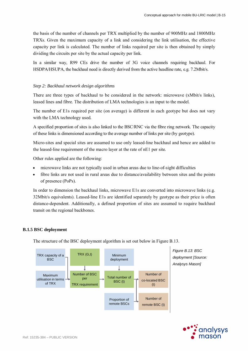
Conceptual approach for mobile BU-LRIC model | B-15
Ref: 15235-384 – PUBLIC VERSION
the basis of the number of channels per TRX multiplied by the number of 900MHz and 1800MHz
TRXs. Given the maximum capacity of a link and considering the link utilisation, the effective
capacity per link is calculated. The number of links required per site is then obtained by simply
dividing the circuits per site by the actual capacity per link.
In a similar way, R99 CEs drive the number of 3G voice channels requiring backhaul. For
HSDPA/HSUPA, the backhaul need is directly derived from the active headline rate, e.g. 7.2Mbit/s.
Step 2: Backhaul network design algorithms
There are three types of backhaul to be considered in the network: microwave (xMbit/s links),
leased lines and fibre. The distribution of LMA technologies is an input to the model.
The number of E1s required per site (on average) is different in each geotype but does not vary
with the LMA technology used.
A specified proportion of sites is also linked to the BSC/RNC via the fibre ring network. The capacity
of these links is dimensioned according to the average number of links per site (by geotype).
Micro-sites and special sites are assumed to use only leased-line backhaul and hence are added to
the leased-line requirement of the macro layer at the rate of nE1 per site.
Other rules applied are the following:
microwave links are not typically used in urban areas due to line-of-sight difficulties
fibre links are not used in rural areas due to distance/availability between sites and the points
of presence (PoPs).
In order to dimension the backhaul links, microwave E1s are converted into microwave links (e.g.
32Mbit/s equivalents). Leased-line E1s are identified separately by geotype as their price is often
distance-dependent. Additionally, a defined proportion of sites are assumed to require backhaul
transit on the regional backbones.
B.1.5 BSC deployment
The structure of the BSC deployment algorithm is set out below in Figure B.13.
TRX (G,t)
Maximum utilisation in terms
of TRX
TRX capacity of a BSC
Minimum deployment
Number of BSC per
TRX requirement
Total number of BSC (t)
Proportion of remote BSCs
Number of
remote BSC (t)
Number of
co-located BSC (t)
Figure B.13: BSC
deployment [Source:
Analysys Mason]

Conceptual approach for mobile BU-LRIC model | B-16
Ref: 15235-384 – PUBLIC VERSION
BSC deployment is driven by two requirements:
the maximum number of TRXs controlled, assuming a maximum utilisation
the minimum number of BSCs deployed in the network (for redundancy). Each of those two
requirements leads to a different number of BSC units: the total number of BSCs corresponds
to the higher of those two values.
A proportion of BSCs are designated as ‘remote’ (i.e. not co-located with an MSC). Additionally,
the BSCs now have AMR capabilities. As explained when dealing with TRXs, this feature allows
for decreased radio resource consumption.
The traffic transiting through collocated BSCs and MSCs is backhauled to the MSC using tie
cables or other cables laid out within the switching site.
The model can keep the flexibility to reflect the potential deployment of remote BSCs. In that
case, the total traffic handled by each remote BSC can be calculated using the total BHE
transceiver traffic. The average BHE traffic handled by each remote BSC is converted into a
channel requirement using the Erlang table. The number of links is then calculated by dividing this
channel requirement by the capacity of a link, adjusted for maximum utilisation. It should be noted
that the capacity of the BSC–MSC transmission depends on where the transcoder equipment is
located. For remote BSCs, the transcoder is assumed to be located in the MSC.
The number of BSC–MSC ports is determined on the basis of the number of BSC–MSC links.
Total outgoing ports for co-located BSCs
Given the total number of co-located BSCs and BHE transceiver traffic, the total number of
outgoing ports for co-located BSCs is calculated. The flow of calculation for co-located BSC ports
is similar to that shown in Figure B.14. The transcoder is assumed to be in the BSC and the co-
located links are not modelled (because this is part of the in-building cat-5 or similar wiring, as
explained in the previous paragraph).

Conceptual approach for mobile BU-LRIC model | B-17
Ref: 15235-384 – PUBLIC VERSION
Incoming and outgoing ports
The incoming ports to the BSC are ports facing the BTS, while the outgoing ports are ports facing
the MSC. Figure B.14 below shows the constituents of the incoming and outgoing ports.
BSC-MSC BHE (t)
BSC-MSC BHE per remote BSC (t)
Remote BSC-MSC E1 utilisation
Remote BSC-MSC E1 capacity
Number of E1 for remote BSC-MSC
links
Number of remote
BSC (t)
BSC-MSC BHE per co-located BSC (t)
Number of E1 for co-located BSC-MSC
links
Number of co-located
BSC (t)
Co-located BSC-MSC E1 utilisation
Co-located BSC-MSC E1 capacity
BSC-MSC BHE (t)
Total E1 outgoing ports
Number of leaded line backhaul E1 links
(t)
Number of microwave backhaul E1 links (t)
Number of fibre backhaul E1 links (t)
Number of co-located backhaul E1 links (t)
Total E1 incoming ports
Remote BSC-MSC links
Figure B.14: Calculation of BSC incoming and outgoing ports and transmission requirements [Source:
Analysys Mason]
The total number of incoming ports into a BSC is the sum of the microwave, leased-line and fibre
backhaul links, while the total number of outgoing ports is the sum of the total number of links for
both remote and co-located BSCs.
B.1.6 3G RNC deployment
The deployment of RNC units is driven by three requirements:
the maximum throughput in Mbit/s (assessed in the downlink direction), assuming a maximum
utilisation
the maximum number of E1 ports connected, assuming a maximum utilisation
the minimum number of RNCs deployed in the network for redundancy.

Conceptual approach for mobile BU-LRIC model | B-18
Ref: 15235-384 – PUBLIC VERSION
Each of those three requirements leads to a different number of RNC units. The total number of
RNCs is the highest of those three values.
The number of RNC incoming ports (ports facing Node-Bs) are directly derived from the number
of backhaul E1 links, including all technologies.
The RNC–MSC links and core-facing E1 or STM1 ports are dimensioned based on the average
RNC downlink throughput, taking into account a utilisation factor that reflects, among other
things, the need for redundant ports and links.
Total downlink Mbit/s in radio layer
RNC throughput max utilisation
Mb/s capacity of a RNC
Number of NodeB-facing RNC ports (t)
Maximum utilisation in terms
of ports
E1 ports capacity of a RNC
Minimum deployment
Number of RNC per
Mb/s requirement
Number of RNC per
Ports requirement
Total number of RNSC (t)
R99 voice Mbit/s in the voice busy hour
R99 downlink Mbit/s in the voice
busy hour
HSDPA Mbit/s in the voice busy hour
Average downlink Mbit/s in radio layer
per RNC Mb/s capacity of core-facing RNC
ports (E1 or STM1)Number of core-facing RNC ports
RNC-MSC link utilisation
RNC-MSC links
Minimum number of core-facing RNC
ports
Figure B.15: RNC dimensioning [Source: Analysys Mason]
B.1.7 MSC (MSC-server and MGW) deployment
In an all-IP network, the MSC is modelled as two separate components: the MSS and the MGW.
MSSs are driven by the voice processing capacity driver (busy-hour call attempts (BHCA))
MGWs are driven by the voice traffic load and the BSC/RNC port requirements, as well as a
typical deployment rule of an MGW pair per MSS.

Conceptual approach for mobile BU-LRIC model | B-19
Ref: 15235-384 – PUBLIC VERSION
Calculation of the number of MSC (MSS) units
In order to support processing demand, the number of MSC (MSS) units required is calculated
from the central processing unit (CPU) capacity, processor utilisation and the demand for MSC
processor time. Figure B.16 below shows the calculation sequence.
BHCA (t)
Maximum utilisation in terms
of BHCA
BHCA capacity of a MSC
Number of MSC per
BHCA requirement
Combined Media gateways
(t)
Combined MSC Servers (t)
Minimum deployment of MSC Servers
Figure B.16: Calculation
of MSC (MSS) units
[Source: Analysys
Mason]
Taking into account the MSC (MSS) processor utilisation, the total number of processors required to
meet the demand can be calculated as the total number of BHms divided by the effective capacity.
B.1.8 Deployment of other network elements
Home location register (HLR)
HLR units are deployed based on average subscribers. Figure B.17 below shows the calculations
used to obtain the number of HLR units required.
HLR utilisation
HLR capacity
(t) = by time
Minimum HLR requiredNumber of HLR units required (t)
Actual HLR capacity
HLR required to support subscribers (t)
Average subscribers (t)
Figure B.17: HLR units
calculation [Source:
Analysys Mason]
A minimum number of two HLR units is typically deployed from the start of operations, to cater
for pre-provisioned prepaid SIMs and redundancy. HLR units have an associated capacity and a
maximum utilisation factor.

Conceptual approach for mobile BU-LRIC model | B-20
Ref: 15235-384 – PUBLIC VERSION
SMSC
The SMSC deployment is driven by SMS throughput demand. Figure B.18 below shows the
calculation flow.
SMSC utilisation
SMSC throughput capacity
(t) = by time
Minimum SMSC requiredNumber of SMSC units required (t)
Actual SMSC capacity
SMS required to support throughput demand (t)
SMS throughput demand BH SMS (t)
Figure B.18: Calculation
of SMSC units [Source:
Analysys Mason]
Dividing the SMS throughput demand by the actual SMSC capacity gives the number of SMSCs
required to support this throughput demand. The number of SMSC units deployed is the higher of
either the SMSCs required to support demand or the minimum SMSC units (one unit).
GPRS/EDGE/UMTS packet data infrastructure
There are three types of equipment specifically deployed for data services, namely PCU, SGSN
and GGSN.
PCU units are added to the GSM BSCs to groom packet data to/from the radio transmission. A
certain number of PCUs are deployed per BSC (if not incorporated within the modern BSC unit).
It is assumed the UMTS RNC intrinsically contains PCU functionality. Figure B.19 below shows
the calculation flow.
(t) = by time
PCU unit capacity Mbit/s
Number of PCUs required for capacity (t)
GPRS traffic BH Mbit/s (t)
Minimum number of PCUs per BSC required
Number of PCU units required (t)
Figure B.19: Calculation
of PCU units [Source:
Analysys Mason]

Conceptual approach for mobile BU-LRIC model | B-21
Ref: 15235-384 – PUBLIC VERSION
The number of PCUs deployed is the maximum of the calculated number of PCUs required for
capacity and the minimum number of PCUs per BSC required (which is one).
Figure B.20 below shows the calculations for SGSN and GGSN deployment, supporting attached
and active packet data subscribers of both 2G and 3G networks. The same calculations are
repeated for 2G, 3G or shared SGSN.
SGSN/GGSN utilisation
SGSN/GGSN capacity
(t) = by time
Minimum SGSN/GGSN required
Number of SGSN/GGSN units required (t)
Actual SGSN/GGSN capacity
SGSN/GGSN required
Connected subscribers/ active PDP contexts in the busy hour (t)
Data traffic demand in the busy hour (t)
Figure B.20: SGSN and
GGSN units calculation
[Source: Analysys
Mason]
The calculations for both SGSN and GGSN deployment are similar. SGSN deployment can be
driven by the number of SAUs in the busy hour, while GGSN deployment can be driven by the
number of active packet data protocol (PDP) contexts in the busy hour. The minimum number of
SGSNs and GGSNs deployed is two, for redundancy reasons.
The model assumes that the operator deploys new platforms, which are typically shared SGSNs
and GGSNs, i.e. used for both GPRS/EDGE and UMTS.
Calculation of PCU-SGSN links (Gb interface)
First, the Gb interface (PCU-SGSN links) is dimensioned in order not to be the network bottleneck, i.e. the capacity needed on the Gb interface is assumed to be equal to the capacity that would be needed if all GPRS channels reserved were simultaneously active on all sectors in the network.
Second, remote Gb traffic is calculated as a proportion of total PCU-SGSN traffic based on the proportion of remote PCUs, which is assumed to be equal to the proportion of remote BSCs.
Remote Gb traffic is then converted into E1 equivalent taking into account the utilisation of remote PCU-SGSN links.

Conceptual approach for mobile BU-LRIC model | B-22
Ref: 15235-384 – PUBLIC VERSION
Finally, the Gb links are added to the BSC-MSC links for the purpose of expressing either in E1 or STM1 equivalents, depending on the capacity needed.
Number of sectors
GPRS/EDGE channels reserved
by sector
GPRS/EDGE channel rate, kbit/s
Total capacity needed on Gb
interface (Mb/s)
Total GPRS/EDGE capacity in radio
network
Proportion of remote BSCs
Remote PCU-SGSN link utilisation
Total remote Gb interface capacity
dimensioned (Mb/s)
Number of remote
BSC (t)
Remote Gb interface capacity dimensioned per
BSC (E1s)
Total E1 equivalents
necessary for Gb interface
Figure 21: Calculation of PCU-SGSN links (Gb interface) [Source: Analysys Mason]
VMS, Intelligent Network, billing system
These network elements are modelled as a single functional unit deployed at the commencement
of operations.
Network management system (NMS)
The network management system is deployed at the start of operations.

Conceptual approach for mobile BU-LRIC model | C-1
Ref: 15235-384 – PUBLIC VERSION Error! Unkn own d oc umen t pro pert y n ame.
Annex C: Glossary
2G Second generation mobile telephony
3G Third generation mobile telephony
AMR Adaptive multi-rate
BHCA Busy hour call attempts
BHE Busy hour Erlangs
BSC Base station controller
BTS Base (transmitter) station
BU Bottom-up
CCA Current cost accounting
CPU Central processing unit
CS Circuit switch
E1 2Mbit/s unit of capacity
GGSN Service GPRS support node
GPRS General packet radio system
GSM Global system for mobile communications
GSN GPRS serving node
HCA Historical cost accounting
HLR Home location register
HSDPA High-speed downlink packet access
HSPA High-speed packet access
HSUPA High-speed uplink packet access
IP Internet Protocol
IRU Indefeasible right to use
LMA Last mile access
LRAIC Long-run average incremental cost
LRIC Long-run incremental cost
LTE Long Term Evolution
MEA Modern equivalent asset
MGW Media gateway
MSC Mobile switching centre
MSS Mobile switching centre server
MTR Mobile termination rate
NMG Network management system
NGN Next-generation network
NPV Net present value
PCU Packet control unit
PDP Packet data protocol
PoI Point of interconnect
PoP Point of presence
PS Packet switch
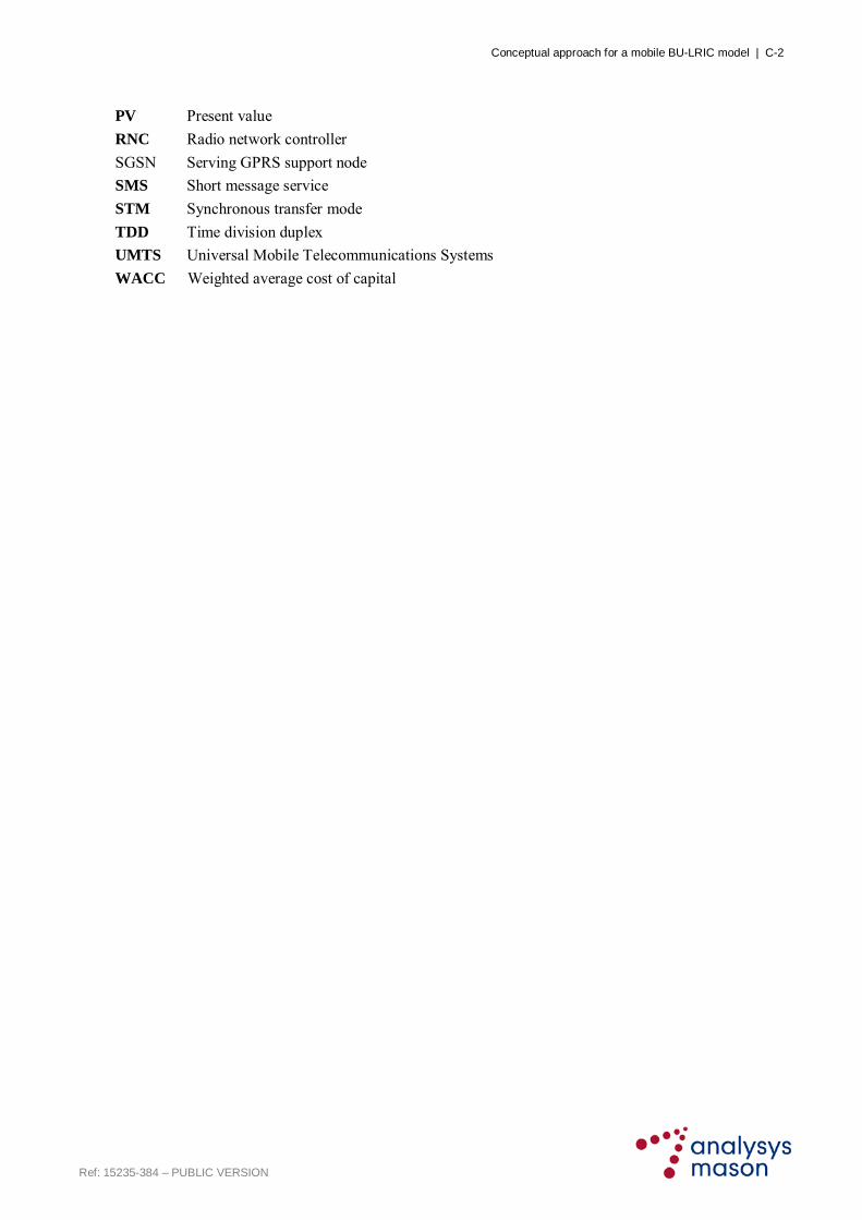
Conceptual approach for a mobile BU-LRIC model | C-2
Ref: 15235-384 – PUBLIC VERSION Error! Unkn own d oc umen t pro pert y n ame.
PV Present value
RNC Radio network controller
SGSN Serving GPRS support node
SMS Short message service
STM Synchronous transfer mode
TDD Time division duplex
UMTS Universal Mobile Telecommunications Systems
WACC Weighted average cost of capital
![[1] H. He, J. Tian, M. Zhao, J. Xue, y K. Lu, «3D Medical ...pegasus.javeriana.edu.co/~CIS1130TK03/documentos/Anexo3... · He, J. Tian, M. Zhao, J. Xue, y K. Lu, «3D Medical Imaging](https://static.documents.pub/doc/80x56/5ad329d57f8b9a92258e0e2a/1-h-he-j-tian-m-zhao-j-xue-y-k-lu-3d-medical-cis1130tk03documentosanexo3he.jpg)


