Animating Pictures with Stochastic Motion Textures Yung-Yu Chuang 1,3 Dan B Goldman 1 Ke Colin Zheng 1 Brian Curless 1 David H. Salesin 1,2 Richard Szeliski 2 1 University of Washington 2 Microsoft Research 3 National Taiwan University (a) Japanese Temple (b) Harbor (c) Boat Studio (d) Argenteuil (e) Sunflowers Figure 1 Sample input images we animate using our technique. The first two pictures are photographs of a Japanese Temple (a) and a harbor (b). The paintings shown in (c) and (d) are Claude Monet’s The Boat Studio and The Bridge at Argenteuil. We also apply our method to Van Gogh’s Sunflower (e) to animate the flowers. (The last three paintings are courtesy of WebMuseum, http://www.ibiblio.org/wm/.) Abstract In this paper, we explore the problem of enhancing still pictures with subtly animated motions. We limit our domain to scenes con- taining passive elements that respond to natural forces in some fash- ion. We use a semi-automatic approach, in which a human user seg- ments the scene into a series of layers to be individually animated. Then, a “stochastic motion texture” is automatically synthesized us- ing a spectral method, i.e., the inverse Fourier transform of a filtered noise spectrum. The motion texture is a time-varying 2D displace- ment map, which is applied to each layer. The resulting warped layers are then recomposited to form the animated frames. The re- sult is a looping video texture created from a single still image, which has the advantages of being more controllable and of gener- ally higher image quality and resolution than a video texture created from a video source. We demonstrate the technique on a variety of photographs and paintings. CR Categories: I.3.3 [Computer Graphics]: Picture/Image Generation—Display algorithms; I.4.9 [Image Processing and Computer Vision]: Applications Keywords: Animation, image-based animation, image-based ren- dering, natural phenomena, physical simulation, video texture 1 Introduction When we view a photograph or painting, we perceive much more than the static picture before us. We supplement that image with our life experiences: given a picture of a tree, we imagine it sway- ing; given a picture of a pond, we imagine it rippling. In effect, we bring to bear a strong set of “priors,” and these priors enrich our perception. http://grail.cs.washington.edu/projects/StochasticMotionTextures/ In this paper, we explore how a set of explicitly encoded priors might be used to animate still images on a computer. The fully au- tomatic animation of arbitrary scenes is, of course, a monumental challenge. In order to make progress, we make the problem easier in two ways. First, we use a semi-automatic, user-assisted approach. In particu- lar, a user segments the scene into a set of animatable layers and assigns certain parameters to each one. Second, we limit our scope to scenes containing passive elements that respond to natural forces in some fashion. We explore a range of passive elements including plants and trees, water, floating objects such as boats, and clouds. The motion of each of these objects is driven by a single natural force, namely, the wind. Although this set of objects and motions may seem limited, they occur in a large variety of pictures and paintings, as shown in Figure 1. We have found that all of these elements can be animated using a unified approach. First, we segment the picture into a set of user- specified layers using Bayesian matting [Chuang et al. 2001]. As each layer is removed from the picture, “inpainting” is used to fill in the resulting hole. Next, the user annotates one or more layers with a motion armature, a line segment which approximates the struc- ture of a layer. Using these constraints, we synthesize a stochastic motion texture using spectral methods [Stam 1995]. Spectral meth- ods work by generating a random noise spectrum in the frequency domain, applying a physically based spectrum filter to that noise, and computing an inverse Fourier transform to create the stochastic motion texture. This motion texture is a time-varying 2D displace- ment map, which is applied to the pixels in the layer. Finally, the warped layers are recomposited to form the animated picture for each frame. The resulting moving picture can be thought of as a kind of video texture [Sch¨ odl et al. 2000]—although, in this case, a video texture created from a single static image rather than from a video source. Thus, these results have potential application wherever video tex- tures do, i.e., in place of still images on Web sites, as screen savers or desktop “wallpapers,” or in presentations and vacation slide shows. In addition, there are several advantages to creating video textures from a static image rather than from a video source. First, because they are created synthetically, they allow greater creative control in their appearance. For example, the wind direction and amplitude
Transcript
Animating Pictures with Stochastic Motion Textures
Yung-Yu Chuang1,3 Dan B Goldman1 Ke Colin Zheng1 Brian Curless1 David H. Salesin1,2 Richard Szeliski2
1University of Washington 2Microsoft Research 3National Taiwan University
(a) Japanese Temple (b) Harbor (c) Boat Studio (d) Argenteuil (e) Sunflowers
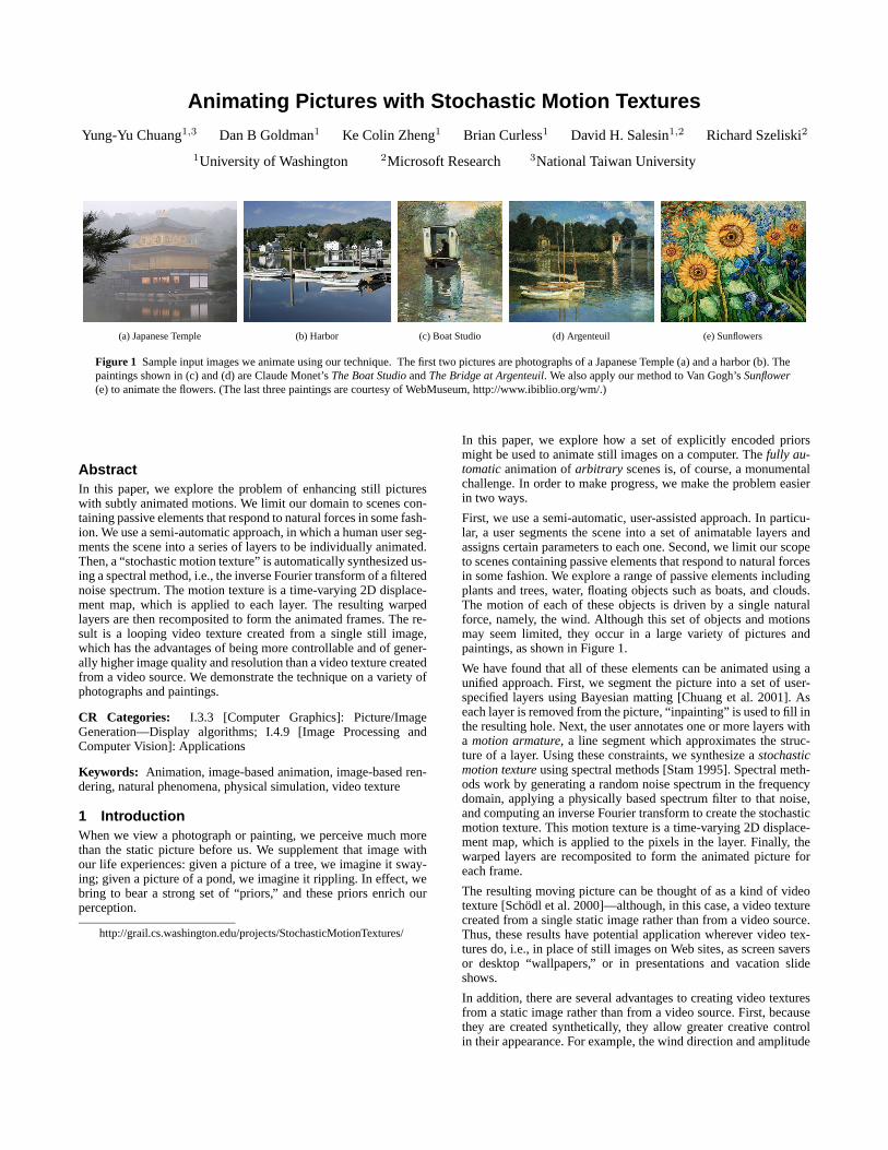
Figure 1 Sample input images we animate using our technique. The first two pictures are photographs of a Japanese Temple (a) and a harbor (b). Thepaintings shown in (c) and (d) are Claude Monet’s The Boat Studio and The Bridge at Argenteuil. We also apply our method to Van Gogh’s Sunflower(e) to animate the flowers. (The last three paintings are courtesy of WebMuseum, http://www.ibiblio.org/wm/.)
AbstractIn this paper, we explore the problem of enhancing still pictureswith subtly animated motions. We limit our domain to scenes con-taining passive elements that respond to natural forces in some fash-ion. We use a semi-automatic approach, in which a human user seg-ments the scene into a series of layers to be individually animated.Then, a “stochastic motion texture” is automatically synthesized us-ing a spectral method, i.e., the inverse Fourier transform of a filterednoise spectrum. The motion texture is a time-varying 2D displace-ment map, which is applied to each layer. The resulting warpedlayers are then recomposited to form the animated frames. The re-sult is a looping video texture created from a single still image,which has the advantages of being more controllable and of gener-ally higher image quality and resolution than a video texture createdfrom a video source. We demonstrate the technique on a variety ofphotographs and paintings.
1 IntroductionWhen we view a photograph or painting, we perceive much morethan the static picture before us. We supplement that image withour life experiences: given a picture of a tree, we imagine it sway-ing; given a picture of a pond, we imagine it rippling. In effect, webring to bear a strong set of “priors,” and these priors enrich ourperception.
In this paper, we explore how a set of explicitly encoded priorsmight be used to animate still images on a computer. The fully au-tomatic animation of arbitrary scenes is, of course, a monumentalchallenge. In order to make progress, we make the problem easierin two ways.
First, we use a semi-automatic, user-assisted approach. In particu-lar, a user segments the scene into a set of animatable layers andassigns certain parameters to each one. Second, we limit our scopeto scenes containing passive elements that respond to natural forcesin some fashion. We explore a range of passive elements includingplants and trees, water, floating objects such as boats, and clouds.The motion of each of these objects is driven by a single naturalforce, namely, the wind. Although this set of objects and motionsmay seem limited, they occur in a large variety of pictures andpaintings, as shown in Figure 1.
We have found that all of these elements can be animated using aunified approach. First, we segment the picture into a set of user-specified layers using Bayesian matting [Chuang et al. 2001]. Aseach layer is removed from the picture, “inpainting” is used to fill inthe resulting hole. Next, the user annotates one or more layers witha motion armature, a line segment which approximates the struc-ture of a layer. Using these constraints, we synthesize a stochasticmotion texture using spectral methods [Stam 1995]. Spectral meth-ods work by generating a random noise spectrum in the frequencydomain, applying a physically based spectrum filter to that noise,and computing an inverse Fourier transform to create the stochasticmotion texture. This motion texture is a time-varying 2D displace-ment map, which is applied to the pixels in the layer. Finally, thewarped layers are recomposited to form the animated picture foreach frame.
The resulting moving picture can be thought of as a kind of videotexture [Schodl et al. 2000]—although, in this case, a video texturecreated from a single static image rather than from a video source.Thus, these results have potential application wherever video tex-tures do, i.e., in place of still images on Web sites, as screen saversor desktop “wallpapers,” or in presentations and vacation slideshows.
In addition, there are several advantages to creating video texturesfrom a static image rather than from a video source. First, becausethey are created synthetically, they allow greater creative controlin their appearance. For example, the wind direction and amplitude
can be tuned for a particular desired effect. Second, consumer-gradedigital still cameras generally provide much higher image qualityand greater resolution than their video camera counterparts. Theseadvantages allow animated stills to be used in new situations suchas animated matte paintings for special effects. Furthermore, theycan be applied to sources that exist only in a static form such aspaintings and historic photographs.
For the most part, the algorithms we describe in this paper are ap-plications of techniques from a variety of disparate sources suchas image matting and inpainting, and physically based animationof natural phenomena. We show how these techniques can be com-bined, seamlessly and synergistically into an easy-to-use system foranimating still images. Thus, our major contributions are in the for-mulation of the overall problem, including the recognition that aninteresting class of phenomena can all be animated attractively via asingle wind source using simple controls; the marshalling of a vari-ety of techniques, most notably stochastic motion textures, to solv-ing this problem; the design of a user interface that allows noviceusers to animate pictures with little or no training; and lastly, a proofof the viability and quality of applying image warping approachesto synthesizing appealing animated pictures.
1.1 Related work
Our goal is to synthesize a stochastic video from a single image.Hence, our work is similar in spirit to the work on video texturesand dynamic textures [Szummer and Picard 1996; Schodl et al.2000; Wei and Levoy 2000; Soatto et al. 2001; Wang and Zhu2003]. Like our work, video textures focus on “quasi-periodic”scenes. However, the inputs to video texture algorithms are shortvideos that can be analyzed to mimic the appearance and dynam-ics of the scene. In contrast, the input to our work is only a singleimage.
Our work is, in spirit, similar to the “Tour Into the Picture” sys-tem developed by Horry et al. [1997]. Their system allows users tomap a 2D image onto a simple 3D box scene based on some inter-actively selected perspective viewing parameters such as vanishingpoints. This approach allows users to interactively navigate into apicture. Criminisi et al. [2000] propose an automated technique thatcan produce similar effects in a geometrically correct way. Morerecently, Oh et al. [2001] developed an image-based depth editingsystem capable of augmenting a photograph with a more compli-cated depth field to synthesize more realistic effects. In our work,instead of synthesizing a depth field to change the viewpoint, weadd motion fields to make the scene change over time.
For certain classes of motions, our system requires the userto specify a motion armature for a layer, and then performsphysically-based simulation on the armature to synthesize a mo-tion field. It is therefore similar to the method of Litwinowicz andWilliams [1994], which uses keyframe line drawings to deform im-ages to create 2D animations. Their system is quite useful for tra-ditional 2D animation. However, their technique is not suitable formodeling the natural phenomena we target because such motionsare difficult to keyframe. Also, they use a smooth scattered datainterpolation to synthesize a motion field without any physical dy-namics.
Our work is also related to the object-based image editing systemproposed by Barrett and Cheney [2002], namely, object selection,matte extraction, and hole filling. Indeed, Barrett et al. have alsodemonstrated how to generate a video from a single image by edit-ing and interpolating keyframes. Like Litwinowicz’s system, the fo-cus is on key-framed rather than stochastic (temporal texture-like)motions.
Freeman et al. [1991] previously attempted to create the illusionof motion in a static image in their “Motion without movement”paper. They apply quadrature pairs of oriented filters to vary the
local phase in an image to give the illusion of motion. While themotion is quite compelling, the band-pass filtered images do notlook photorealistic.
Even earlier, at the turn of the 20th century, people painted out-door scenes on pieces of masked vellum paper and used series ofsequentially timed lights to create the illusion of descending wa-terfalls [Hathaway et al. 2003]. People still make this kind of de-vice, which is often called a kinetic waterfall. Another example ofa simple animated picture is the popular Java program, Lake ap-plet, which takes a single image and perturbs the image with a setof simple ripples [Griffiths 1997]. Though visually pleasing, theseresults often do not look realistic because of their lack of physicalproperties.
Working on an inverse problem to ours, Sun et al. [2003] proposea video-input driven animation (VIDA) system to extract physi-cal parameters such as wind speed from real video footage. Theythen use these parameters to drive the physical simulation of syn-thetic objects to integrate them consistently with the source video.They estimate physical parameters from observed displacements;we synthesize displacements using a physical simulation based onuser-specified parameters. They target a similar set of natural phe-nomena to those we study: plants, waves, and boats, which can allbe explained as harmonic oscillations.
To simulate dynamics, we use physically-based simulation tech-niques previously developed in computer graphics for modelingnatural phenomena. For waves, we use the Fourier wave model tosynthesize a time-varying height field. Mastin et al. [1987] were thefirst to introduce statistical frequency-domain wave models fromoceanography into computer graphics. In a similar way, we synthe-size stochastic wind fields [Shinya and Fournier 1992; Stam andFiume 1993] by applying a different spectrum filter. When apply-ing the wind field to trees, since the force is oscillatory in nature, thecorresponding motions are also periodic and can be solved more ro-bustly and efficiently in the frequency domain [Stam 1997; Shinyaet al. 1998].
Aoki et al. [1999] coupled physically-based animations of plantswith image morphing techniques as an efficient alternative to ex-pensive physically-based plant simulation and synthesis. However,they only demonstrate their concept on synthetic images. In ourwork, we target real pictures and use our approach as a way to syn-thesize video textures for stochastic scenes.
Our system requires users to segment an image into layers. To sup-port seamless composites, a soft alpha matte for each layer is re-quired. We use recently proposed interactive image matting algo-rithms to extract alpha mattes from the input image [Ruzon andTomasi 2000; Chuang et al. 2001]. To fill in holes left behind af-ter removing each layer, we use an inpainting algorithm [Bertalmioet al. 2000; Criminisi et al. 2003; Jia and Tang 2003; Drori et al.2003].
1.2 OverviewWe begin with a system overview that describes the basic flow ofour system (Section 2). We then address our most important sub-problem, namely synthesizing a stochastic motion texture (Sec-tion 3). Finally, we discuss our results (Section 4) and end withconclusions and ideas for future work.
2 System overviewGiven a single image, how can we generate a continuously movinganimation quickly and easily? One possibility is to use a keyframe-based approach, as did Litwinowicz and Williams [1994]. However,such an approach is problematic for naıve users: specifying the mo-tions is complex, and achieving any kind of movement resemblingphysical realism is quite difficult. Another straightforward approachis to use compositions of sinusoids to create oscillatory motions
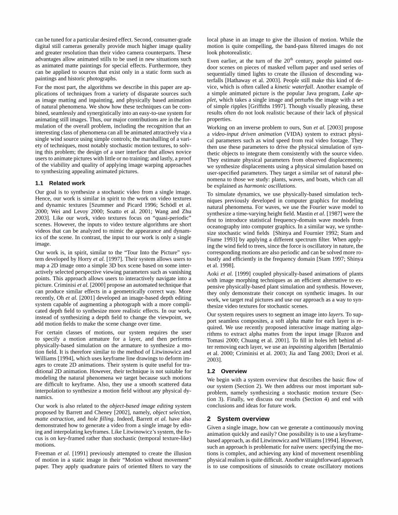
Figure 2 Overview of our system. The input still image (a) is manually segmented into several layers (b). Each layer Li is then animated with adifferent stochastic motion texture di(t) (c). Finally, the animated layers Li(t) (d) are composited back together to produce the final animation I(t)(e).
[Griffiths 1997], but the resulting effect may not maintain a viewer’sinterest over more than a short period of time, on account of its pe-riodicity and predictability.
The approach we ultimately settled upon — which has the advan-tages of being quite simple for users to specify, and of creatinginteresting, complex, and plausibly realistic motion — is to breakthe image up into several layers and to then synthesize a differ-ent motion texture1 for each layer. A motion texture is essentiallya time-varying displacement map defined by a motion type, a setof motion parameters, and in some cases a motion armature. Thisdisplacement map d(p, t) is a function of pixel coordinates p andtime t. Applying it directly to an image layer L results in a forwardwarped image layer L′ such that
L′(p + d(p, t)) = L(p) (1)
However, since forward mapping is fraught with problems such asaliasing and holes, we actually use inverse warping, defined as
L′(p) = L(p + d′(p, t)) (2)
We denote this operation as L′ = L ⊗ d′.
We could compute the inverse displacement map d′ from d usingthe two-pass method suggested by Shade et al. [1998]. Instead,since our motion fields are all very smooth, we simply dilate themby the extent of the largest possible motion and reverse their sign.
With this notation in place, we can now describe the basic workflowof our system (Figure 2), which consists of three steps: layering andmatting, motion specification and editing, and finally rendering.
Layering and matting. The first step, layering, is to segmentthe input image I into layers so that, within each layer, the samemotion texture can be applied. For example, for the painting in Fig-ure 2(a), we have the following layers: one for each of the water,sky, bridge and shore; one for each of the three boats; and one foreach of the eleven trees in the background (Figure 2(b)). To accom-plish this, we use an interactive object selection tool such as a paint-ing tool or intelligent scissors [Mortensen and Barrett 1995]. Thetool is used to specify a trimap for a layer; we then apply Bayesian
1We use the terms motion texture and stochastic motion texture inter-changeably in this paper. The term motion texture was also used by Li et.al [2002] to refer to a linear dynamic system learned from motion capturedata.
matting to extract the color image and a soft alpha matte for thatlayer [Chuang et al. 2001].
Because some layers will be moving, occluded parts of the back-ground might become visible. Hence, after extracting a layer, weuse an enhanced inpainting algorithm to fill the hole in the back-ground behind the foreground layer. We use an example-based in-painting algorithm based on the work of Criminisi et al. [2003] be-cause of its simplicity and its capacity to handle both linear struc-tures and textured regions.
Note that the inpainting algorithm does not have to be perfect sinceonly pixels near the boundary of the hole are likely to become vis-ible. We can therefore accelerate the inpainting algorithm by con-sidering only nearby pixels in the search for similar patches. Thisshortcut may sacrifice some quality, so in cases where the automaticinpainting algorithm produces poor results, we provide a touch-upinterface with which a user can select regions to be repainted. Theautomatic algorithm is then reapplied to these smaller regions us-ing a larger search radius. We have found that most significant in-painting artifacts can be removed after only one or two such brush-strokes. Although this may seem less efficient than a fully automaticalgorithm, we have found that exploiting the human eye in this sim-ple fashion can produce superior results in less than half the timeof the fully automatic algorithm. Note that if a layer exhibits largemotions (such as a wildly swinging branch), artifacts deep insidethe inpainted regions behind that layer may be revealed. In prac-tice, these artifacts may not be objectionable, as the motion tends todraw attention away from them. When they are objectionable, theuser has the option of improving the inpainting results.
After the background image has been inpainted, we work on thisimage to extract the next layer. We repeat this process from theclosest layer to the furthest layer to generate the desired number oflayers. Each layer Li contains a color image Ci, a matte αi, and acompositing order zi. The compositing order is presently specifiedby hand, but could in principle be automatically assigned with theorder in which the layers are extracted.
Motion specification and editing. The second component ofour system lets us specify and edit the motion texture for each layer.Currently, we provide the following motion types: trees (swaying),water (rippling), boats (bobbing), clouds (translation), and still (nomotion). For each motion type, the user can tune the motion param-eters and specify a motion armature, where applicable. We describethe motion parameters and armatures in more detail for each motiontype in Section 3.
Since all of the motions we currently support are driven by thewind, the user controls a single wind speed and direction, which isshared by all the layers. This allows all the layers to respond to thewind consistently. Our motion synthesis algorithm is fast enoughto animate a half-dozen layers in real-time. Hence, the system canprovide instant visual feedback to changes in motion parameters,which makes motion editing easier. Each layer Li has its own mo-tion texture, di, as shown in Figure 2(c).
Rendering. During the rendering process, for each time in-stance t and layer Li, a displacement map di(t) is synthesized.(Here, we have dropped the dependencies of Li and di on p fornotational conciseness.) This displacement map is then applied toCi and αi to obtain Li(t) = Li(0)⊗di(t) (Figure 2(d)). Notice thatthe displacement is evaluated as an absolute displacement of the in-put image I(0) rather than a relative displacement of the previousimage I(t − 1). In this way, repeated resampling and numericalerror accumulation are avoided.
Finally, all the warped layers are composited together from back tofront to synthesize the frame at time t, I(t) = L1(t) ⊕ L2(t) ⊕. . . ⊕ Ll(t), where z1 ≥ z2 · · · ≥ zl and ⊕ is the standard overoperator [Porter and Duff 1984] (Figure 2(e)).
3 Stochastic motion texturesIn this section, we describe our approach to synthesizing thestochastic motion textures that drive the animated image. We firstdescribe the basic principles on which our system is based (Sec-tion 3.1). We then describe the details of each motion type, i.e., trees(Section 3.2), water (Section 3.3), bobbing boats (Section 3.4), andclouds (Section 3.5).
3.1 Stochastic modeling of natural phenomenaMany natural motions can be viewed as harmonic oscillations [Sunet al. 2003], and, indeed, hand-crafted superpositions of a smallnumber of sinusoids have often been used to approximate naturalphenomena for computer graphics. However, this simple approachhas some limitations, as we discovered after experimenting withthis idea. First of all, it is tedious to tune the parameters to producethe desired effects. Second, it is hard to create motions for eachlayer that are consistent with one another since they lack a physicalbasis. Lastly, the resulting motions do not look natural since theyare strictly periodic — irregularity actually plays a central role inmodeling natural phenomena.
One way to add randomness is to introduce a noise field. Intro-ducing this noise directly into the temporal or spatial domain oftenleads to erratic and unrealistic simulations of natural phenomena.Instead, we simulate noise in the frequency domain, and then sculptthe spectral characteristics to match the behaviors of real systemsthat have intrinsic periodicities and frequency responses. Specificspectrum filters need to be applied to model specific phenomena,leading to so-called spectral methods [Stam 1995].
The spectral method for synthesizing a stochastic field has threesteps: (1) generate a complex Gaussian random field in the fre-quency domain, (2) apply a domain-specific spectrum filter, and(3) compute the inverse Fourier transform to synthesize a stochas-tic field in the time or frequency domain. A nice property of thismethod is that the synthesized stochastic field can be tiled seam-lessly. Hence, we only need to synthesize a patch of reasonable sizeand tile it to produce a much larger stochastic signal. This tiling ap-proach works reasonably well if the size of the patch is large enoughto avoid objectionable repetition. Furthermore, each layer can use apatch of a different size, which obscures any repetitive motion thatmay remain in individual layers.
To realistically model natural phenomena, the filter should belearned from real-world data. For the phenomena we simulate,
plants and waves, such experimental data and statistics are avail-able from other fields, e.g., structural engineering and oceanogra-phy, and have already been used by the graphics community to cre-ate synthetic imagery [Shinya and Fournier 1992; Stam and Fiume1993; Mastin et al. 1987]. After experimenting with several differ-ent variants published in both the computer graphics and simulationliterature, we selected the following set of techniques to synthesizestochastic motion textures that are both realistic and easy to control.
3.2 Plants and treesThe branches and trunks of trees and plants can be modeled as phys-ical systems with mass, damping, and stiffness properties. The driv-ing function that causes branches to sway is typically wind [Stam1997]. Our goal is to model the spectral filtering due to the dy-namics of the branches applied to the spectrum of the driving windforce.To model the physics of branches, we take the simplified view intro-duced by Sun et al. [2003]. In particular, the motion of each branchis constrained by a motion armature; a 2D line segment parameter-ized by u, which ranges from 0 to 1. This line segment is drawnby the user for each layer. Note that, to model a correct mechanicalstructure, the line segment may need to extend outside the image.Displacements of the tip of the branch dtip(t) are taken to be per-pendicular to the line segment. Modal analysis indicates that thedisplacement perpendicular to the line for other points along thebranch can be simplified to the form:
d(u, t) =[
1
3u4 − 4
3u3 + 2u2
]
dtip(t) (3)
We approximate the (scalar) displacement of the tip in the directionof the projected wind force as a damped harmonic oscillator:
dtip(t) + γdtip(t) + 4π2f2o dtip(t) = w(t)/m (4)
where m is the mass of the branch, fo = k/m is the naturalfrequency of the system, and γ = c/m is the velocity dampingterm [Sun et al. 2003]. These parameters have a more intuitivemeaning than the damping (c) and stiffness (k) terms found in moretraditional formulations. The driving force w(t) is derived from thewind force incident on the branch, as detailed below.Taking the temporal Fourier transform F{} of equation (4) and not-ing that F{dtip(t)} = i2πfF{dtip(t)}, we arrive at
−4π2f2Dtip(f) + i2πγfDtip(f) + 4π2f2o Dtip(f) =
W (f)
m(5)
where i =√−1 and Dtip(f) and W (f) are the Fourier transforms
of dtip(t) and w(t), respectively. Solving for Dtip(f) and express-ing the result in complex exponential notation gives
Dtip(f) =W (f)ei2πθ
2πm{
[2π (f2 − f2o )]2 + γ2f2
}1/2(6)
where W (f) is the Fourier transform of the driving wind force, afunction of frequency f , as defined in equations (8) and (9) below.The phase shift θ is given by
tan θ =γf
2π (f2 − f2o )
(7)
Next, we model the forcing spectrum for wind. An empirical modelmade from experimental measurements [Simiu and Scanlan 1986,p. 55] indicates that the temporal power spectrum of the wind ve-locity at a point takes the following form:
PV (f) ∼ vmean
(1 + κf/vmean)5/3(8)
where vmean is the mean wind speed and κ is generally a functionof altitude, which we take to be a constant. The velocity spectrumis given by the square root of the power spectrum. We thereforemodulate a random Gaussian noise field G(f) with the velocityspectrum to compute the spectrum of a particular (random) windvelocity field:
V (f) = G(f)√
PV (f) (9)
The force due to the wind is complicated by the presence of turbu-lence [Feynman et al. 1964, Fig. 41-4], but can be generally mod-eled as a drag force proportional to the squared wind velocity. How-ever, in our experiments, we have found that making the wind forcedirectly proportional to wind velocity produces more pleasing re-sults.
Finally, we assemble Equations (6)-(9) to construct the spectrum ofthe tip displacement Dtip(f), take the inverse Fourier transform togenerate the tip displacement dtip(t), and distribute the displace-ment over the branch according to equation (3). We apply the dis-placement as a rotation of each point about the root position of thebranch. The displacements of points in the layer away from the mo-tion armature are given by the displacement of the point on the ar-mature that is the same distance from the root.
The user can control the resulting motion appearance by indepen-dently changing the mean wind speed vmean and the natural (oscil-latory) frequency fo, mass m, and velocity damping term γ of eachbranch.
3.3 WaterWater surfaces belong to another class of natural phenomena thatexhibit oscillatory responses to natural forces like wind. In this sec-tion we describe how one can specify a 3D water plane in a photo-graph and then define the mapping of water height out of that planeto displacements in image space. We then describe how to synthe-size water height variations, again using a spectral method.
The motion armature for water is simply a plane; we assume thatthe image plane is the xy plane and the water surface is the xz plane.To correctly model the perspective effect, the user roughly specifieswhere the plane is. This perspective transformation M can be fullyspecified by the focal length and the tilt of the camera, which canbe visualized by drawing the horizon [Criminisi et al. 2000].
After specifying the 3D water plane, the water is animated usinga time-varying height field h(q, t), where q = (xq, y0, zq)
T is apoint on the water plane, and y0 = 0 is the elevation of the wa-ter plane. To convert the height field h to the displacement mapd(p, t), for each pixel p we first find that pixel’s correspondingpoint q = Mp on the water plane. We then add the synthesizedheight h(q, t) as a vertical displacement, which gives us a pointq′ = (xq, h(q, t), zq)
T . We then project q′ back to the image planeto get p′ = M−1q′. The displacement vector for d(p, t) = p′ − pis therefore
d(p, t) = M−1[Mp + (0, h(Mp, t), 0)T ] − p (10)
Note that p and p′ are affine points, d is a vector, and M is a 3 × 3matrix.
The above model is technically correct if we want to displace ob-jects on the surface of the water. In reality, the shimmer in the wateris caused by local changes in surface normals. Therefore, a morephysically realistic approach would be to use normal mapping, i.e.,to convert the surface normals computed from the spatial gradi-ents of h(q, t) into two-dimensional displacements of the reflectedrays. However, we have found that applying this normal mappingapproach without a 3-dimensional model of the surrounding envi-ronment produces confusing distortions compared to our current
approach, which generally produces pleasing, realistic-looking re-flections as long as the wave amplitude is relatively small.
To synthesize a time-varying height field for the water, weuse the user-specified wind velocity to synthesize a height fieldmatching the statistics of real ocean waves, as described byMastin et al. [1987]. Note that this approach deals only withocean waves, which are gravity waves. Although it does not phys-ically describe short-length waves, non-wind-generated waves onrivers/brooks/streams or large waves on shallow water, it gives plau-sible results for our application.
The spectrum filter we use for waves is the Phillips spec-trum [Tessendorf 2001], which is a power spectrum describing theexpected square amplitude of waves across all spatial frequencies s
PH(s) ∼ e[−1/(sL)2]
s4|s · vmean|2 (11)
where s = |s|, and L = v2mean/g, and g is the gravitational con-
stant, and s and vmean are normalized spatial frequency and winddirection vectors in the xz plane, respectively. (We denote 2D vec-tors in boldface.)
The square root of the power spectrum describes the amplitude ofwave heights, which we can use to filter a random Gaussian noisefield G(s):
H0(s) = aG(s)√
PH(s) (12)
where a is a constant of proportionality and H0 is an instance of theheight field which we can now animate by introducing time-varyingphase. However, waves of different spatial frequencies move at dif-ferent speeds. The relationship between the spatial frequency andthe phase velocity is described by the well-known dispersion rela-tion,
ω(s) =√
gs (13)
The time varying height spectrum can thus be expressed as
H(s, t) = H0(s)eiω(s)t + H∗
0 (−s)e−iω(s)t (14)
where H∗
0 is the complex conjugate of H0 [Tessendorf 2001].We can now compute the height field at time h(q, t) as the two-dimensional inverse Fourier transform of H(s, t) with respect tospatial frequencies s. We take the generated height field and tilethe water surface using a scale parameter, β, to control the spatialfrequency.
To recap the process, given the wind speed and direction, we syn-thesize a spectrum filter using equation (11) and apply it to a spatialGaussian noise field to obtain an initial height field (12). This heightfield is then animated using equation (14) to synthesize the Fouriertransform H(s, t) of the height field h(q, t) at time t. Taking theinverse Fourier transform, we recover the height field, use it to tilethe water plane and substitute it into equation (10) to synthesizemotion texture di at time t.
There are thus several motion parameters related to water: windspeed, wind direction, the size of the tile N , the amplitude scalea, and the spatial frequency scale β. The wind speed and direc-tion are controlled globally for the whole animation. We find that atile of size N = 256 usually produces nice looking results for thesizes of images we used. Users can change a to scale the height ofthe waves/ripples. Finally, scaling the frequencies by β changes thescale at which the wave simulation is being done. Simulating at alarger frequency scale gives a rougher look, while a smaller scalegives a smoother look. Hence, we call β the roughness in our userinterface.
3.4 BoatsWe approximate the motion of a bobbing boat by a 2D rigid trans-formation composed of a translation for heaving and a rotation forrolling. A boat moving on the surface of open water is almost al-ways in oscillatory motion [Sun et al. 2003]. Hence, the simplestmodel is to assign a sinusoidal translation and a sinusoidal rota-tion. However, this often looks fake. In principle, we could builda simple model for the boat, convert the height field of water intoa force interacting with the hull, and solve the dynamics equationfor the boat to estimate its displacement. However, since our goalis to synthesize a quickly computable solution, we directly use theheight field of the wave to move the boat, as follows.
We let the user select a line close to the bottom of the boat. Then, wesample several points qi along the line and assume these points areon the water plane surrounding the boat. At time t, for each point qi,we look up its displacement vector d(pi, t) (10) and calculate thecorresponding position p′
i of pi at time t as pi+d(pi, t). Finally, weuse linear regression to fit a line through the displaced positions.The position and orientation of the fitted line then determine theheaving and rolling of the boat.
3.5 CloudsAnother common element for scenic pictures is clouds. In principle,clouds could also be modeled as a stochastic process. However, weneed the stochastic process to match the clouds in the image at somepoint, which is harder. Since clouds often move very slowly andtheir motion does not attract too much attention, we simply assigna translational motion field to them. We extend the clouds outsidethe image frame to create a cyclic texture using our inpainting algo-rithm, since their motion in one direction will create holes that wehave to fill.
4 ResultsWe have developed an interactive system that supports matting, in-painting, motion editing, and previewing the results. We have ap-plied our system to several photographs and famous paintings. Theaccompanying video provides a sense of the user interface for cre-ating the animated pictures, as well as a demonstration of the ani-mated results.
Table 1 summarizes the number of layers of each type created forthe five animated pictures shown in Figure 1, the motion specifica-tion, along with the time that it took a user to perform the mattingand in-painting steps (which are interleaved in the process, and thusdifficult to separate in time), and the playback speeds. Generally thematting and in-painting steps take the large majority of the time. Inall cases, the animated paintings take from a little under an hour toa few hours to create. Note that two of the animated pictures whosetimings are presented above, “Boat Studio” and “Sunflowers,” werecreated by a complete novice user who only had a few minutes ofinstruction before beginning work on the pictures. We provide play-back speeds for our current unoptimized software implementation:Our code presently takes no special advantage of graphics hard-ware, but all of the operations could be readily mapped to GPUs,thereby greatly increasing frame rates.
For the Japanese Temple (Figure 1(a)), we model a total of 10branches on the left and the right. We use a small wave amplitude(a = 1.0) and high roughness (β = 200) to give the ripples a fine-grained look. For the harbor picture in Figure 1(b), we animate thewater and have nine boats swing with the water. The cloud and skyare animated using a translational motion field.
Figure 1(c)-(e) shows three paintings we have animated. Our tech-nique works reasonably well with paintings, probably because inthis situation we are even less sensitive to anything that does notlook perfectly realistic. For Claude Monet’s painting in Figure 1(c),we animate the water with lower amplitude roughness to keep the
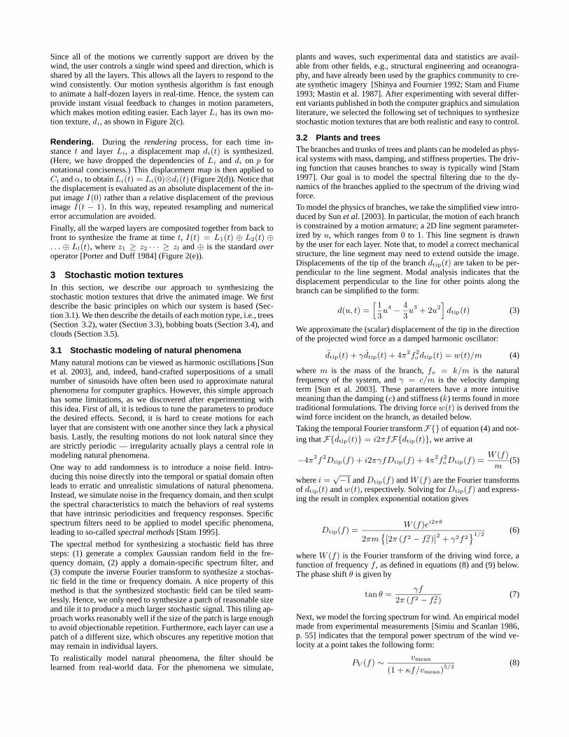
strokes intact. We also let the boat sway with the water. Another ofMonet’s paintings, shown in Figure 1(d), is a more complex exam-ple, with more than twenty layers. We use this example to demon-strate that we can change the appearance of the water by control-ling the physical parameters. In Figure 3, we show the appearanceof the water under different wind speeds, directions, and simulationscales.
For Van Gogh’s sunflower painting (Figure 1(e)), we use ourstochastic wind model to animate the twenty-five plant layers. Witha simple sinusoidal model, the viewer usually can quickly figure outthat the plants swing in synchrony, and the motion loses a lot of itsinterest. With the stochastic wind model, the flowers’ motions de-correlate in phase and the resulted animation is more appealing. Wealso experimented with a very small amount of scaling along thebranch armature in order to simulate foreshortening of the flowersas they move in and out of the image plane.
5 Conclusion and future workIn this paper, we have described an approach for animating stillpictures of outdoor scenes that contain dynamic elements that re-spond to natural forces in a simple quasi-periodic fashion. We seeour work as just a first step in the larger problem of animating amuch more general class of pictures.
Before we began this work, it was not at all clear whether it wouldbe possible to make still images come to life as animated scenes. Webelieve our judicious selection and enhancement of recently devel-oped matting, inpainting, stochastic motion synthesis, image warp-ing, and compositing algorithms provides an effective and easy-to-use system for generating realistic animations from static images.
We point out that our choice of techniques is especially well-suitedto this problem, in that a relatively high-quality composite anima-tion can be produced even when the results of each automated stepare of objectively lower quality. First, the use of matting produceslayers that are color-coherent along their boundaries, even if the re-sulting matte does not follow object boundaries. When in motion,these layers often seem perceptually plausible even when techni-cally incorrect. Second, the limited amount of displacement we seekto introduce implies that the inpainting process can be relativelylow-quality and still produce seamless composites. This allows usto use heuristic measures to reduce the search space and speed upthe inpainting process. Finally, we do not ask end users to keyframeanimations, but rather influence the scene in physical, easily under-stood terms, such as wind speed and direction. We provide a userinterface that is accessible to users at all levels. Many users arealready familiar with matting and inpainting processes from com-mercial products such as Photoshop, and the additional burden ofassigning “canned” motion types is minimal.
Our system currently makes a number of assumptions that wewould like to relax. For example, we assume that the elements of theinput image are in their equilibrium positions. This is often not thecase, e.g., for a scene with water that already has ripples. Indeed,an interesting challenge would be to use these ripples to estimatethe water motion, unwarp the reference image and then animate itcorrectly. In addition, we currently ignore the effects of shadows,transparency, and reflections. For example, the reflections of theboat move with the deformations of the water, but do not accountfor any additional motion due to the boat’s bobbing up and down.When the motion is large, the results are less realistic. One solutionwould be to segment out reflections, transparent layers and shadowssomehow, and let them move with the casting objects accordingly.
Many of our approximations limit the plausibility of very large-scale motions, in which pixels are warped more than a few dozenpixels from their source position. For example, we simulate boatsrolling as a 2D rigid motion. It might be possible to fake a slight3D rotation with a non-rigid distortion, to allow for more plausible
(a) composite (b) lower wind speed (c) wind of different direction (d) rougher water surface
Figure 3 We can control the appearance of water surface by adjusting some physical parameters such as wind speed. We show one of the composites(a) as the reference, in which the wind blow at 5 m/s in z direction. We decrease the wind speed to 3 m/s (b) and change the wind direction to be alongz axis (c). In (d), we change the scale of the simulation to render water with finer ripples.
Trees Water Boats Clouds Still Layering Animating Rendering ResolutionJapanese Temple 10 1 0 0 2 45 m 10 m 7 fps 900x675
Harbor 0 2 9 1 5 90 m 10 m 3.8 fps 900x600Boat Studio 0 1 1 0 1 30 m 10 m 10 fps 600x692Argenteuil 16 1 3 1 3 120 m 15 m 4.1 fps 800x598Sunflowers 25 0 0 0 1 210 m 20 m 5.1 fps 576x480
Table 1 The number of layers of each type for each of the five examples in Figure 1, along with approximate times in minutes for a user to performthe layering steps (including matting and inpainting), animating step (including motion specification and editing), and playback speeds.
large-scale motions. Very large warps of the water surface can ap-pear distorted due to warping from outside the image boundaries,and when the water waves become large enough under very windyconditions, we expect to see a number of additional real-world ef-fects such as water “lapping up” against the shore or boats, “white-caps,” splashes, or other turbulent surface effects.
Our method currently works best for trees at a distance. For nearbytrees, it is presently difficult and tedious to segment the leaf andbranch structure properly. It would also be interesting to add the“shimmering” effect of leaves blowing in the wind by applying tur-bulent flow fields within the tree layers.
There are other classes of motion that could be modeled using asimilar approach. We imagine that waterfalls, ocean waves, flyingbirds and other small animals, flame, and smoke may all be pos-sible. For example, waterfalls could perhaps be animated using atechnique similar to ”motion without movement” [Freeman et al.1991]. Ocean waves could be simulated using stochastic models,although matching the appearance of the source image poses someinteresting challenges. Flying birds and other small animals couldbe animated using ideas from video sprites [Schodl et al. 2000]. Webelieve that it might also be possible to animate fluids like flame orsmoke. However, this would require a constrained stochastic simu-lation, since the state of simulation should resemble the appearanceof the input image. Recent advances in controlling smoke simula-tion by keyframes could be used for this purpose [Treuille et al.2003].
In our system, all the layers are hooked up together to a syntheticwind force. Currently, the same mean wind velocity is applied ev-erywhere in the scene. It would be straightforward to extend the for-mulation to handle complete vector fields of evolving wind forcesin order to provide a more realistic style of animation such as mov-ing gusts of wind. In addition, we could add more controllability sothat the users could interact with trees individually.
Currently, we use physically-based simulation to synthesize a para-metric motion field, but the quality of the motion could potentiallybe improved using learning algorithms to transfer motion from sim-ilar type of objects in videos.
Furthermore, our motion model addresses only a restricted range ofmotions. We imagine future systems might handle transitions be-tween different types of motion, animation to or from a rest state,
water features such as streams that move continuously in a single di-rection, and transitions between different scene states and/or typesof motion (e.g. weather changing from calm to stormy, skies chang-ing from clear to cloudy, boats traveling to and from the horizon,etc.).Our system presently requires a fair amount of user interaction. Wehope to further reduce the time and effort to create these anima-tions by exploiting continued advances in intelligent image selec-tion and matting algorithms such as GrabCut [Rother et al. 2004]or Lazy Snapping [Li et al. 2004]. Furthermore, an automated orsemi-automated region classification to identify features such asforeground tree branches and water would enable a much moreautomated process. For example, one could imagine automaticallyidentifying the “white water” of a waterfall, and then automaticallyanimating the waterfall. For a lake with a simple boundary, such asin Figure 1(a), it might also be possible to automatically segmentthe the water region by identifying reflections.Another possibility would be to use multiple pictures as input.Most modern digital cameras have a “motor-drive” mode that al-lows users to take high-resolution photographs at a restricted sam-pling rate, around 1–3 frames per second. From such a set of pho-tographs we might be able to automatically segment a picture intoseveral coherently moving regions and figure out the motion param-eters from the sample still images. It would also be interesting tocombine high-resolution stills with lower-resolution video to pro-duce attractive animations. Our approach could also be combinedwith “Tour into the picture” to provide an even richer experience,with the ability to move the camera and less constrained perspectiveplanes.In conclusion, we have shown the ease with which it is possibleto breathe life into pictures, based on recently developed matting,inpainting, and stochastic modeling algorithms. We hope that ourwork will inspire other to explore the creative possibilities in thisrich domain.
AcknowledgmentsThe authors wish to thank Wil Li for narrating our video, and MiraDontcheva for user-testing our segmentation and inpainting sytem.We would also like to thank the reviewers for their helpful com-ments. This work was supported by the University of WashingtonAnimation Research Labs, Washington Research Foundation, NSF
grant CCR-0098005, NSC 94-2213-E-002-051, NSC 93-2622-E-002-033 and an industrial gift from Microsoft Research.
ReferencesAOKI, M., SHINYA, M., TSUTSUGUCHI, K., AND KOTANI, N. 1999.
Dynamic texture: Physically-based 2D animation. In ACM SIGGRAPH1999 Conference Sketches and Applications, 239.
BARRETT, W. A., AND CHENEY, A. S. 2002. Object-based image editing.ACM Transactions on Graphics 21, 3, 777–784.
BERTALMIO, M., SAPIRO, G., CASELLES, V., AND BALLESTER, C.2000. Image inpainting. In Proceedings of ACM SIGGRAPH 2000, 417–424.
CHUANG, Y.-Y., CURLESS, B., SALESIN, D. H., AND SZELISKI, R.2001. A Bayesian approach to digital matting. In Proceedings of IEEEInternational Conference on Computer Vision and Pattern Recognition(CVPR) 2001, vol. II, 264–271.
CRIMINISI, A., REID, I. D., AND ZISSERMAN, A. 2000. Single viewmetrology. International Journal of Computer Vision 40, 2, 123–148.
CRIMINISI, A., PEREZ, P., AND TOYAMA, K. 2003. Object removalby exemplar-based inpainting. In Proceedings of IEEE InternationalConference on Computer Vision and Pattern Recognition (CVPR) 2003,vol. II, 721–728.
DRORI, I., COHEN-OR, D., AND YESHURUN, H. 2003. Fragment-basedimage completion. ACM Transactions on Graphics 22, 3, 303–312.
FEYNMAN, R. P., LEIGHTON, R. B., AND SANDS, M. 1964. The FeynmanLectures On Physics, Volume II: Mainly Electromagnetism and Matter.Addison Wesley, Reading, Mass.
FREEMAN, W. T., ADELSON, E. H., AND HEEGER, D. J. 1991. Mo-tion without movement. Computer Graphics (Proceedings of ACM SIG-GRAPH 91) 25, 4, 27–30.
GRIFFITHS, D., 1997. Lake java applet. http://www.jaydax.co.uk/tutorials/laketutorial/dgclassfiles.html.
HATHAWAY, T., BOWERS, D., PEASE, D., AND WENDEL, S., 2003.http://www.mechanicalmusicpress.com/history/pianella/p40.htm.
HORRY, Y., ANJYO, K.-I., AND ARAI, K. 1997. Tour into the picture:using a spidery mesh interface to make a nimation from a single image.In Proceedings of ACM SIGGRAPH 1997, 225–232.
JIA, J., AND TANG, C.-K. 2003. Image repairing: Robust image synthesisby adaptive ND tensor voting. In Proceedings of IEEE InternationalConference on Computer Vision and Pattern Recognition (CVPR) 2003,vol. I, 643–650.
LI, Y., WANG, T., AND SHUM, H.-Y. 2002. Motion texture: a two-levelstatistical model for character motion synthesis. ACM Transactions onGraphics 21, 3, 465–472.
LI, Y., SUN, J., TANG, C.-K., AND SHUM, H.-Y. 2004. Lazy snapping.ACM Transactions on Graphics 23, 3, 303–308.
LITWINOWICZ, P., AND WILLIAMS, L. 1994. Animating images withdrawings. In Proceedings of ACM SIGGRAPH 1994, 409–412.
MASTIN, G. A., WATTERBERG, P. A., AND MAREDA, J. F. 1987. Fouriersynthesis of ocean scenes. IEEE Computer Graphics and Applications7, 3, 16–23.
MORTENSEN, E. N., AND BARRETT, W. A. 1995. Intelligent scissors forimage composition. In Proceedings of ACM SIGGRAPH 1995, 191–198.
OH, B. M., CHEN, M., DORSEY, J., AND DURAND, F. 2001. Image-basedmodeling and photo editing. In Proceedings of ACM SIGGRAPH 2001,433–442.
PORTER, T., AND DUFF, T. 1984. Compositing digital images. ComputerGraphics (Proceedings of ACM SIGGRAPH 84) 18, 4, 253–259.
ROTHER, C., KOLMOGOROV, V., AND BLAKE, A. 2004. Grabcut — inter-active foreground extraction using iterated graph cuts. ACM Transactionson Graphics 23, 3, 309–314.
RUZON, M. A., AND TOMASI, C. 2000. Alpha estimation in natural im-ages. In Proceedings of IEEE International Conference on ComputerVision and Pattern Recognition (CVPR) 2000, 18–25.
SCHODL, A., SZELISKI, R., SALESIN, D. H., AND ESSA, I. 2000. Videotextures. In Proceedings of ACM SIGGRAPH 2000, 489–498.
SHADE, J., GORTLER, S., HE, L.-W., AND SZELISKI, R. 1998. Layereddepth images. In Proceedings of ACM SIGGRAPH 1998, 231–242.
SHINYA, M., AND FOURNIER, A. 1992. Stochastic motion – motion underthe influence of wind. Computer Graphics Forum 11, 3, 119–128.
SHINYA, M., MORI, T., AND OSUMI, N. 1998. Periodic motion synthesisand Fourier compression. The Journal of Visualization and ComputerAnimation 9, 3, 95–107.
SIMIU, E., AND SCANLAN, R. H. 1986. Wind Effects on Structures. JohnWiley & Sons.
SOATTO, S., DORETTO, G., AND WU, Y. N. 2001. Dynamic textures.In Proceedings of IEEE International Conference on Computer Vision(ICCV) 2001, 439–446.
STAM, J., AND FIUME, E. 1993. Turbulent wind fields for gaseous phe-nomena. In Proceedings of ACM SIGGRAPH 1993, 369–376.
STAM, J. 1995. Multi-Scale Stochastic Modelling of Complex Natural Phe-nomena. PhD thesis, Dept. of Computer Science, University of Toronto.
STAM, J. 1997. Stochastic dynamics: Simulating the effects of turbulenceon flexible structures. Computer Graphics Forum 16, 3, 159–164.
SUN, M., JEPSON, A. D., AND FIUME, E. 2003. Video input drivenanimation (VIDA). In Proceedings of IEEE International Conference onComputer Vision (ICCV) 2003, 96–103.
SZUMMER, M., AND PICARD, R. W. 1996. Temporal texture modeling.In Proceedings of IEEE International Conference on Image Processing(ICIP) 1996, vol. 3, 823–826.
TESSENDORF, J. 2001. Simulating ocean water. ACM SIGGRAPH 2001course notes No. 47 Simulating Nature: Realistic and Interactive Tech-niques.
TREUILLE, A., MCNAMARA, A., POPOVIC, Z., AND STAM, J. 2003.Keyframe control of smoke simulations. ACM Trans. Graph. 22, 3, 716–723.
WANG, Y., AND ZHU, S. C. 2003. Modeling textured motion: Particle,wave and sketch. In Proceedings of IEEE International Conference onComputer Vision (ICCV) 2003, 213–220.
WEI, L.-Y., AND LEVOY, M. 2000. Fast texture synthesis using tree-structured vector quantization. In Proceedings of ACM SIGGRAPH2000, 479–488.