AnintroductiontoCopulas - Åbo...

An introduction to Copulas


Carlo Sempi

Dipartimento di Matematica “Ennio De Giorgi”Università del Salento

Lecce, [email protected]

The 33rd Finnish Summer School on Probability Theory andStatistics, June 6th–10th, 2011

C. Sempi An introduction to Copulas. Tampere, June 2011.


Outline

1 Historical Introduction

2 Preliminaries

3 Copulæ

4 Sklar’s theorem

5 Copulæ and stochastic measures


An introduction to CopulasHistorical Introduction

The beginning of the story

The history of copulas may be said to begin with Fréchet (1951).Fréchet’s problem: given the distribution functions Fj(j = 1, 2, . . . , d) of d r.v.’s X1,X2, . . . ,Xd defined on the sameprobability space (Ω,F ,P), what can be said about the setΓ(F1,F2, . . . ,Fd ) of the d–dimensional d.f.’s whose marginals arethe given Fj?

H ∈ Γ(F1, . . . ,Fd )⇐⇒ H(+∞, . . . ,+∞, t,+∞, . . . ,+∞) = Fj(t)

The set Γ(F1, . . . ,Fd ) is called the Fréchet class of the Fj ’s.Notice Γ(F1, . . . ,Fd ) 6= ∅ since, if X1,X2, . . . ,Xd are independent,then

H(x1, x2, . . . , xd ) =d∏

j=1

Fj(xj).

But, it was not clear which the other elements of Γ(F1, . . . ,Fd )were.C. Sempi An introduction to Copulas. Tampere, June 2011.


Bibliography–1

For Fréchet’s work see, e.g.,

M. Fréchet, Sur les tableaux de corrélation dont les margessont donnés, Ann. Univ. Lyon, Science, 4, 13–84 (1951)

G. Dall’Aglio, Fréchet classes and compatibility of distributionfunctions, Symposia Math., 9, 131–150 (1972)

In this latter paper Dall’Aglio studies under which conditions thereis just one d.f. belonging to Γ(F1,F2).



Enters Sklar

In 1959, Sklar obtained the most important result in this respect,by introducing the notion, and the name, of a copula, and provingthe theorem that now bears his name.



Correspondence with Fréchet

He and Bert Schweizer had been making progress in their work onstatistical metric spaces, to the extent that Menger suggested itwould be worthwhile to communicate their results to Fréchet.Fréchet was interested, and asked to write an announcement forthe Comptes Rendus. This lead to an exchange of letters betweenSklar and Fréchet, in the course of which Fréchet sent Sklar severalpackets of reprints, mainly dealing with the work he and hiscolleagues were doing on distributions with given marginals. Thesereprints were important for much of the subsequent work. At thetime, though, the most significant reprint for Sklar was that ofFéron (1956).



Sklar–2

Féron, in studying three-dimensional distributions had introducedauxiliary functions, defined on the unit cube, that connected suchdistributions with their one-dimensional margins. Sklar saw thatsimilar functions could be defined on the unit d–cube for all d ≥ 2and would similarly serve to link d–dimensional distributions to theirone–dimensional margins. Having worked out the basic propertiesof these functions, he wrote about them to Fréchet, in English.



Sklar–3

Fréchet asked Sklar to write a note about them in French. Whilewriting this, Sklar decided he needed a name for these functions.Knowing the word “copula” as a grammatical term for a word orexpression that links a subject and predicate, he felt that this wouldmake an appropriate name for a function that links amultidimensional distribution to its one-dimensional margins, andused it as such. Fréchet received Sklar’s note, corrected onemathematical statement, made some minor corrections to Sklar’sFrench, and had the note published by the Statistical Institute ofthe University of Paris (Sklar, 1959).



A curiosity

Curiously, it should be noted that in that paper, the author “AbeSklar” is named as “M. Sklar” (should it be intended as“Monsieur”?)



Lack of a proof

The proof of Sklar’s theorem was not given in (Sklar, 1959), but asketch of it was provided in (Sklar, 1973). (see also (Schweizer &Sklar, 1974)), so that for a few years practitioners in the field hadto reconstruct it relying on the hand–written notes by Sklar himself;this was the case, for instance, of the present speaker. It should bealso mentioned that some “indirect” proofs of Sklar’s theorem(without mentioning copula) were later discovered by Moore &Spruill and Deheuvels.



For about 15 years, all the results concerning copulas were obtainedin the framework of the theory of Probabilistic Metric spaces(Schweizer & Sklar, 1974). The event that arose the interest of thestatistical community in copulas occurred in the mid seventies,when Bert Schweizer, in his own words (Schweizer, 2007),

quite by accident, reread a paper by A. Rényi, entitledOn measures of dependence and realized that [he] couldeasily construct such measures by using copulas.

The first building blocks were the announcement by Schweizer &Wolff in the Comptes Rendus de l’Académie des Sciences (1976)and Wolff’s Ph.D. Dissertation at the University of Massachusettsat Amherst (1977). These results were presented to the statisticalcommunity in (Schweizer & Wollf, 1981) (see also (Wolff, 1980)).



However, for several other years, Chapter 6 of the 1983 book bySchweizer & Sklar, devoted to the theory of Probabilistic metricspaces, was the main source of basic information on copulas. Againin Schweizer’s words from (Schweizer, 2007),

After the publication of these articles and of the book. . . the pace quickened as more . . . students and colleaguesbecame involved. Moreover, since interest in questions ofstatistical dependence was increasing, others came to thesubject from different directions. In 1986 the enticinglyentitled article “The joy of copulas” by C. Genest and R.CMacKay (1986), attracted more attention.



Finance

At end of the nineties, the notion of copulas became increasinglypopular. Two books about copulas appeared and were to becomethe standard references for the following decade. In 1997 Joepublished his book on multivariate models, with a great partdevoted to copulas and families of copulas. In 1999 Nelsenpublished the first edition of his introduction to copulas (reprintedwith some new results in 2006).But, the main reason of this increased interest has to be found inthe discovery of the notion of copulas by researchers in severalapplied field, like finance. Here we should like briefly to describe thisexplosion by quoting Embrechts’s comments (Embrechts, 2009).



Embrechts

. . . the notion of copula is both natural as well as easyfor looking at multivariate d.f.’s. But why do we witnesssuch an incredible growth in papers published starting theend of the nineties (recall, the concept goes back to thefifties and even earlier, but not under that name)? Here Ican give three reasons: finance, finance, finance. In theeighties and nineties we experienced an explosivedevelopment of quantitative risk managementmethodology within finance and insurance, a lot of whichwas driven by either new regulatory guidelines or thedevelopment of new products . . . . Two papers more thanany others “put the fire to the fuse”: the . . . 1998 RiskLabreport (Embrechts et al., 2002) and at around the sametime, the Li credit portfolio model (Li, 2001).



Today

The advent of copulas in finance originated a wealth ofinvestigations about copulas and, especially, applications of copulas.At the same time, different fields like hydrology discovered theimportance of this concept for constructing more flexiblemultivariate models. Nowadays, it is near to impossible to give acomplete account of all the applications of copulas to the manyfields where they have be used.Since the field is still in fieri, it is important from time to time tosurvey the progresses that have been achieved, and the newquestions that they pose. The aim of this talk is to survey therecent literature.



Today–2

To quote Schweizer again:

The “era of i.i.d.” is over: and when dependence istaken seriously, copulas naturally come into play. Itremains for the statistical community at large to recognizethis fact. And when every statistics text contains asection or a chapter on copulas, the subject will havecome of age.


An introduction to CopulasPreliminaries

Random variables and vectors

When a r.v. X = (X1,X2, . . . ,Xd ) is given, two problems areinteresting:

to study the probabilistic behaviour of each one of itscomponents;to investigate the relationship among them.

It will be seen how copulas allow to answer the second one of theseproblems in an admirable and thorough way.It is a general fact that in probability theory, theorems are proved inthe probability space (Ω,F ,P), while computations are usuallycarried out in the measurable space (Rd

,B(Rd)) endowed with the

law of the random vector X.



Distribution functions

The study of the law PX is made easier by the knowledge of thedistribution function(=d.f.), as defined here.Given a random vector X = (X1,X2, . . . ,Xd ) on the probabilityspace (Ω,F ,P), its distribution function FX : Rd → I is defined by

FX(x1, x2, . . . , xd ) = P(∩d

i=1 Xi ≤ xi)

(1)

if all the xi ’s are in R, while:FX(x1, x2, . . . , xd ) = 0, if at least one of the arguments equals−∞FX(+∞,+∞, . . . ,+∞) = 1.



C–volume

A d–box is a cartesian product

[a,b] =d∏

j=1

[aj , bj ],

where, for every index j ∈ 1, 2, . . . , d, 0 ≤ aj ≤ bj ≤ 1.For a function C : Id → I, the C–volume VC of the box [a,b] isdefined via

VC ([a,b]) :=∑v

sign(v)C (v)

where the sum is carried over all the 2d vertices v of the box [a,b];here

sign(v) =

1, if vj = aj for an even number of indices,−1, if vj = aj for an odd number of indices.



Properties of distribution functions

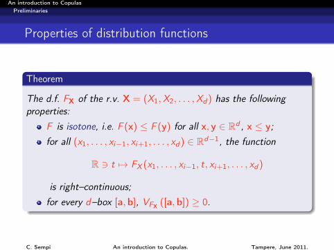
Theorem

The d.f. FX of the r.v. X = (X1,X2, . . . ,Xd ) has the followingproperties:

F is isotone, i.e. F (x) ≤ F (y) for all x, y ∈ Rd , x ≤ y;for all (x1, . . . , xi−1, xi+1, . . . , xd ) ∈ Rd−1, the function

R 3 t 7→ FX (x1, . . . , xi−1, t, xi+1, . . . , xd )

is right–continuous;for every d–box [a,b], VFX ([a,b]) ≥ 0.



Marginals

Let F be a d–dimensional d.f. (d ≥ 2). Let σ = (j1, . . . , jm) asubvector of (1, 2, . . . , d), 1 ≤ m ≤ d − 1. We call σ–marginal of Fthe d.f. Fσ : Rm → I defined by setting d −m arguments of Fequal to +∞, namely, for all x1, . . . , xm ∈ R,

Fσ(x1, . . . , xm) = F (y1, . . . , yd ),

where, for every j ∈ 1, 2, . . . , d, yj = xj if j ∈ j1, . . . , jm, andyj = +∞ otherwise.In particular, when σ = j, F(j) is usually called 1–dimensionalmarginal and it is denoted by Fj .If F is the d.f. of the r.v. ~X = (X1,X2, . . . ,Xd ), then theσ–marginal of F is the d.f. of the subvector (Xj1 , . . . ,Xjm).


An introduction to CopulasCopulæ

The definition

DefinitionFor d ≥ 2, a d–dimensional copula (shortly, a d–copula) is ad–variate d.f. on Id whose univariate marginals are uniformlydistributed on I.

Each d -copula may be associated with a r.v. U = (U1,U2, . . . ,Ud )such that Ui ∼ U(I) for every i ∈ 1, 2, . . . , d and U ∼ C .Conversely, any r.v. whose components are uniformly distributed onI is distributed according to some copula.The class of all d–copulas will be denoted by Cd .



A characterization

Theorem

A function C : Id → I is a copula if, and only if, the followingproperties hold:

for every j ∈ 1, 2, . . . , d, C (u) = uj when all thecomponents of u are equal to 1 with the exception of the j–thone that is equal to uj ∈ I;C is isotonic, i.e. C (u) ≤ C (v) for all u, v ∈ Id such thatu ≤ v;C is d–increasing.



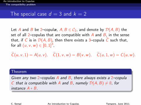
The special case d = 2

Explicitly, a bivariate copula is a function C : I2 → I such that∀u ∈ [0, 1] C (u, 0) = C (0, u) = 0∀u ∈ [0, 1] C (u, 1) = C (1, u) = ufor all u, u′, v , v ′ in I with u ≤ u′ and v ≤ v ′

C (u′, v ′)− C (u′, v)− C (u, v ′) + C (u, v) ≥ 0

This last inequality is referred to as the rectangular inequality; afunction that satisfies it is said to be 2–increasing.



Consequences

C (u) = 0 for every u ∈ Id having at least one of itscomponents equal to 0(The 1–Lipschitz property): for all u, v ∈ Id ,

|C (u)− C (v)| ≤d∑

i=1

|ui − vi |.

Cd is a compact set in the set C (Id , I) of all continuousfunctions from Id into I equipped with the topology ofpointwise convergence.Pointwise and uniform convergence are equivalent in Cd .



Examples–1

The independence copula Πd (u) = u1 u2 · · · ud associated witha random vector U = (U1,U2, . . . ,Ud ) whose components areindependent and uniformly distributed on I.The comonotonicity copula Mind (u) = minu1, u2, . . . , udassociated with a vector U = (U1,U2, . . . ,Ud ) of r.v.’suniformly distributed on I and such that U1 = U2 = · · · = Udalmost surely.The countermonotonicity copulaW2(u1, u2) = maxu1 + u2 − 1, 0 associated with a bivariatevector U = (U1,U2) of r.v.’s uniformly distributed on I andsuch that U1 = 1− U2 almost surely.



Examples–2: Convex combinations

Convex combinations of copulas: Let U1 and U2 be twod–dimensional r.v.’s on (Ω,F ,P) distributed according to thecopulas C1 and C2, respectively. Let Z be a Bernoulli r.v. such thatP(Z = 1) = α and P(Z = 2) = 1− α for some α ∈ I. Supposethat U1, U2 and Z are independent. Now, consider thed–dimensional r.v. U∗

U∗ = σ1(Z ) U1 + σ2(Z ) U2

where, for i ∈ 1, 2, σi (x) = 1, if x = i , σi (x) = 0, otherwise.Then, U∗ is distributed according to the copula αC1 + (1− α)C2.



Examples–3

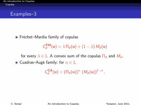
Fréchet–Mardia family of copulas

CFMd (u) = λΠd (u) + (1− λ)Md (u)

for every λ ∈ I. A convex sum of the copulas Πd and Md .Cuadras–Augé family; for α ∈ I,

CCAd (u) = (Πd (u))α (Md (u))1−α ,



The derivatives

Consider a bivariate copula C ∈ C2. For every v ∈ I, the functions

I 3 t → C (t, v)

I 3 t → C (v , t)

are increasing; therefore, their first derivatives exists almosteverywhere with respect to Lebesgue measure and are positive,where they exist. Because of the Lipschitz condition, they are alsobounded above by 1

0 ≤ D1 C (s, t) ≤ 1 0 ≤ D2C (s, t) ≤ 1 a.e.

where

D1 C (s, t) :=∂C (s, t)

∂sand D2 C (s, t) :=

∂C (s, t)

∂t



A useful formula

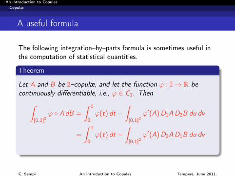
The following integration–by–parts formula is sometimes useful inthe computation of statistical quantities.

Theorem

Let A and B be 2–copulæ, and let the function ϕ : I→ R becontinuously differentiable, i.e., ϕ ∈ C1. Then∫

[0,1]2ϕ AdB =

∫ 1

0ϕ(t) dt −

∫[0,1]2

ϕ′(A)D1AD2B du dv

=

∫ 1

0ϕ(t) dt −

∫[0,1]2

ϕ′(A)D2AD1B du dv



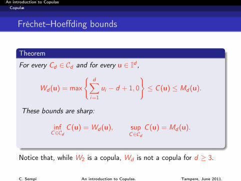
Fréchet–Hoeffding bounds

Theorem

For every Cd ∈ Cd and for every u ∈ Id ,

Wd (u) = max

d∑

i=1

ui − d + 1, 0

≤ C (u) ≤ Md (u).

These bounds are sharp:

infC∈Cd

C (u) = Wd (u), supC∈Cd

C (u) = Md (u).

Notice that, while W2 is a copula, Wd is not a copula for d ≥ 3.



The marginals of a copula

A marginal of an d–copula C is obtained by setting some of itsargument equal 1. A k–marginal of C , k < d , is obtained bysetting exatly d − k arguments equal to 1; therefore, there are(

dk

)k–marginals of the d–copula C .In particular, the d 1–marginals are easily computed:

C (1, 1, . . . , 1, uj , 1, . . . , 1) = uj (j = 1, 2, . . . , d)


An introduction to CopulasSklar’s theorem

Sklar’s Theorem

TheoremGiven an d–dimensional d.f. H there exists an d–copula C suchthat for all (x1, x2, . . . , xd ) ∈ Rn

H(x1, x2, . . . , xd ) = C (F1(x1),F (x2), . . . ,Fd (xd )) (2)

The copula C is uniquely defined on∏d

j=1 ran Fj and is thereforeunique if all the marginals are continuous.Conversely, if F1, F2,. . . , Fd are d (1–dimensional) d.f.’s, then thefunction H defined through eq. (2) is an d–dimensional d.f..



How to obtain a copula from a joint d.f.

Given a d–variate d.f. F , one can derive a copula C . Specifically,when the marginals Fi are continuous, C can be obtained by meansof the formula

C (u1, u2, . . . , ud ) = F (F−11 (u1),F−12 (u2), . . . ,F−1d (ud )),

where F−1i denoted the pseudo–inverse of Fi ,

F−1i (s) = inft | Fi (t) ≥ s.

Thus, copulæ are essentially a way for transforming the r.v.(X1,X2 . . . ,Xd ) into another r.v.

(U1,U2, . . . ,Ud ) = (F1(X1),F2(X2), . . . ,Fd (Xd ))

having the margins uniform on I and preserving the dependenceamong the components.C. Sempi An introduction to Copulas. Tampere, June 2011.


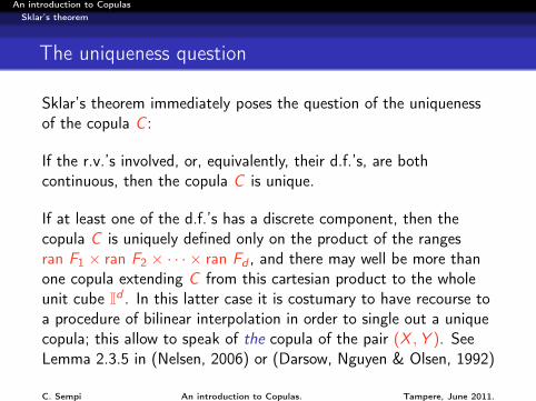
The uniqueness question

Sklar’s theorem immediately poses the question of the uniquenessof the copula C :

If the r.v.’s involved, or, equivalently, their d.f.’s, are bothcontinuous, then the copula C is unique.

If at least one of the d.f.’s has a discrete component, then thecopula C is uniquely defined only on the product of the rangesran F1 × ran F2 × · · · × ran Fd , and there may well be more thanone copula extending C from this cartesian product to the wholeunit cube Id . In this latter case it is costumary to have recourse toa procedure of bilinear interpolation in order to single out a uniquecopula; this allow to speak of the copula of the pair (X ,Y ). SeeLemma 2.3.5 in (Nelsen, 2006) or (Darsow, Nguyen & Olsen, 1992)



Comments

Notice that in many papers where copulæ are applied there isoften hidden the assumption that the r.v.’s involved arecontinuous; this avoids the uniqueness question.If all the d.f.’s involved are continuous then to each joint d.f. inthe Fréchet class Γ(F1,F2, . . . ,Fd ) there corresponds a uniqued–copula C ∈ Cd ; otherwise, to each H ∈ Γ(F1,F2, . . . ,Fd )there corresponds the set of copulas in Cd that coincide on

d∏j=1

ran Fj



Comments–2

The second part of Sklar’s theorem is very easy to prove, but it isextremely important for the applications; it is, in fact, the veryfoundation of all the models built on copulas. Models are builtaccording to the following scheme:

the d rv’s X1,X2, . . . ,Xd are individually described by their1–dimensional d.f.’s F1,F2, . . . ,Fd

then a copula C ∈ Cd is introduced; this contains every pieceof information about the dependence relationship among ther.v.’s X1,X2, . . . ,Xd , independently of the choice of themarginals F1,F2, . . . ,Fd .

In particular, copulas can serve for modelling situations where adifferent distribution is needed for each marginal, providing a validalternative to several classical multivariate d.f.’s such Gaussian,Pareto, Gamma, etc.. This fact represents one of the mainadvantage of the copula’s idea.C. Sempi An introduction to Copulas. Tampere, June 2011.


Caution–2

Sklar’s theorem should be used with some caution when themargins have jumps. In fact, even if there exists a copularepresentation for non–continuous joint d.f.’s, it is no longerunique. In such cases, modelling and interpreting dependencethrough copulas needs some caution. The interested readers shouldrefer to the paper (Marshall, 1996) and to the in–depth discussionby Genest and Nešlehová (2007).



Survival copulæ

Sklar’s Theorem can be formulated in terms of survival functionsinstead of d.f.’s. Specifically, given a r.v. X = (X1,X2, . . .Xd ) withjoint survival function F and univariate survival marginals F i

(i = 1, 2, . . . , d), for all (x1, x2, . . . , xn) ∈ Rd

F (x1, x2, . . . , xd ) = C(F 1(x1),F 2(x2), . . . ,F d (xd )

).

for some copula C , usually called the survival copula of X (thecopula associated with the survival function of X).



Survival copulæ–2

In particular, let C be the copula of X and letU = (U1,U2, . . . ,Ud ) be a vector such that U ∼ C . Then,

C (u) = C (1− u1, 1− u2, . . . , 1− ud ),

where C (u) = P(U1 > u1,U2 > u2, . . . ,Ud > ud ) is the survivalfunction associated with C , explicitly given by

C (u) = 1 +d∑

k=1

(−1)k∑

1≤i1<i2<···<ik≤n

Ci1i2···ik (ui1 , ui2 , . . . , uik ),

with Ci1i2··· ,ik denoting the marginal of C related to (i1, i2, · · · , ik).



Singular and absolutely continuous components

For simplicity’s sake, we consider here only the case d = 2.Every copula C ∈ C2 may be expressed in the form

C = Cac + Cs

where Cac is absolutely continuous and Cs is singular.

For an absolutely continuous copula C one has a density c such that

C (u, v) =

∫I2c(s, t) ds dt =

∫ 1

0ds∫ 1

0c(s, t) dt

The density c is found by differentiation

c(u, v) = D1D2C (u, v) =∂2C (u, v)

∂u ∂va.e.



Singular and absolutely continuous components–2

The presence of a singular component in a copula often causesanalytical difficulties. Nevertheless, there are specific applications inwhich this presence is actually a useful feature; for instance, indefault models described by two random variables X and Y , thefact that the event X = Y may have non–zero probabilityimplies, on the one hand, the existence of a singular component intheir copula, and, on the other hand, the possibility of joint defaultsof X and Y .



A special case

Notice, however, that, as a consequence of the Lipschitz condition,for every copula C ∈ C2 and for every v ∈ I, both functionst 7→ C (t, v) and t 7→ C (v , t) are absolutely continuous so that

C (t, v) =

∫ t

0c1,v (s) ds and C (v , t) =

∫ t

0c2,v (s) ds

This latter representation has so far found no application.Notice also that it possible to prove that, for a 2–copula C ,

D1D2C = D2D1C a.e.



Examples–1

Both the copulæ W2 and M2 are singular:M2 uniformly spreads the probability mass on the maindiagonal v = u (u ∈ I) of the unit square;W2 uniformly spreads the probability mass on the oppositediagonal v = −u (u ∈ I) of the unit square.

The product copula Π2(u, v) := u v is absolutely continuous and itsdensity π is given by

π(u, v) = 1I2(u, v)



Rank–invariant property

TheoremLet X = (X1, . . . ,Xd ) be a r.v. with continuous d.f. F , univariatemarginals F1, F2,. . . , Fd , and copula C. Let T1,. . . ,Td be strictlyincreasing functions from R to R. Then C is also the copula of ther.v. (T1(X1), . . . ,Td (Xd )).

the study of rank statistics – insofar as it is the studyof properties invariant under such transformations – maybe characterized as the study of copulas andcopula-invariant properties.

(Schweizer & Wolff, 1981)



Independence

TheoremLet (X1,X2, . . . ,Xd ) be a r.v. with continuous joint d.f. F andunivariate marginals F1,. . . , Fd . Then the copula of (X1, . . . ,Xd ) isΠd if, and only if, X1,. . . , Xd are independent.



Comonotonicity and countermonotonicity

Theorem

Let (X1,X2, . . . ,Xd ) be a r.v. with continuous joint d.f. F andunivariate marginals F1,. . . ,Fd . Then the copula of (X1, . . . ,Xd ) isMd if, and only if, there exists a r.v. Z and increasing functionsT1,. . . ,Td such that X = (T1(Z ), . . . ,Td (Z )) almost surely.

Theorem

Let (X1,X2) be a r.v. with continuous d.f. F and univariatemarginals F1, F2. Then (X1,X2) has copula W2 if, and only if, forsome strictly decreasing function T , X2 = T (X1) almost surely.



Stochastic measures

Definition

A measure µ on the measurable space (Id ,B(Id )) will said to bestochastic if, for every Borel set A and for every j ∈ 1, 2, . . . , d,

µ(I× · · · × I︸︷︷︸j−1

×A× I× · · · × I) = λ(A),

where λ denotes the (restriction to B(I) of the) Lebesgue measure.


An introduction to CopulasCopulæ and stochastic measures

Copulæ and stochastic measures

TheoremEvery copula C ∈ Cd induces a stochastic measure µC on themeasurable space (Id ,B(Id )) defined on the rectangles R = [a,b]contained in Id , by

µC (R) := VC ([a,b]) .

Conversely, to every stochastic measure µ on (Id ,B(Id )) therecorresponds a unique copula Cµ ∈ Cd defined by

Cµ(u) := µ ([0,u]) .



Markov operators

DefinitionGiven two probability spaces (Ω1,F2,P1) and (Ω2,F2,P2), a linearoperator T : L∞(Ω1)→ L∞(Ω2) is said to be a Markov operator if

T is positive, viz. Tf ≥ 0 whenever f ≥ 0;T1 = 1 (here 1 denotes the constant function f ≡ 1);E2(Tf ) = E1(f ) for every function f ∈ L∞(Ω1) (Ej denotesthe expectation in the probability space (Ωj ,Fj ,Pj) (j = 1, 2))

TheoremEvery Markov operator T : L∞(Ω1)→ L∞(Ω2) has an extension toa bounded operator T : Lp(Ω1)→ Lp(Ω2) for every p ≥ 1.



Copulæ and Markov operators

Theorem

For every copula C ∈ C2 the operator TC defined on L1(I) via

(TC f ) (x) :=ddx

∫ 1

0D2C (x , t) f (t) dt

is a Markov operator on L∞(I).Conversely, for every Markov operator T on L1(I) the function CTdefined on I2 via

CT (x , y) :=

∫ x

0

(T1[0,y ]

)(s) ds

is a 2–copula.



Examples

(TW2 f ) (x) = f (1− x)

(TM2 f ) (x) = f (x)

(TΠ2 f ) (x) =

∫ 1

0f dλ

Theorem

For the adjoint (TC )† of the Markov operator TC in the space Lp

with p ∈ ]1,+∞[ one has (TC )† = TCT , where the transpose CT

of the copula C is defined by CT (x , y) := C (y , x).



The extension to the case d > 2

For d > 2, consider the factorization Id = Ip × Iq, whered = p + q. While for d = 2 there is only one possible factorization,p = 1 and q = 1, this factorization is not unique when d > 2.Let C ∈ Cd be given; it induces a probability measure µC on(Id ,B(Id )). Denote the marginals of µC on (Ip,B(Ip)) and on(Iq,B(Iq)) by µp and µq, respectively.Given a decomposition d = p + q, there is a unique Markovoperator T : L∞(Ip)→ L∞(Iq) associated with µC and, hence,with the copula C . Therefore, to every copula C ∈ Cd therecorrespond as many Markov operators as there are solutions innatural numbers p and q of the Diophantine equation p + q = d .Since the number of these solutions is d − 1, there are d − 1possible different Markov operators corresponding to a d–copulawhen d ≥ 3.




Carlo Sempi






Outline

1 Copulæ and Measure–preserving transformations

2 Construction of copulas

3 Shuffles of Min

4 Archimedean copulæ

5 How many Archimedean copulæ are there?

6 Copulæ and Brownian motion


An introduction to CopulasCopulæ and Measure–preserving transformations

Measure–preserving transformations

(Ω,F , µ) and (Ω′,F ′, ν) — two measure spaces.f : Ω→ Ω′ is a measure–preserving transformations (=MPT) if

∀B ∈ F ′ f −1(B) ∈ F∀B ∈ F ′ µ

(f −1(B)

)= ν(B)

From now on (Ω,F , µ) = (Ω′,F ′, ν) = (I,B(I), λ)B(I) — the Borel sets Iλ — the (restriction) of Lebesgue measure to B(I).



Copulæ and MPT’s

TheoremIf f1, f2,. . . , fd are MPT’s, the function Cf1,f2,...,fd : In → I definedby

Cf1,f2,...,fd (x1, x2, . . . , xd ) := λ(f −11 [0, x1] ∩ · · · ∩ f −1d [0, xd ]

)is a copula. Conversely, for every d–copula C ∈ Cd , there exist dMPT’s f1, f2,. . . fd such that

C = Cf1,f2,...,fd .

This representation is not unique: if ϕ is another MPT on I, then

Cf1,f2,...,fd = Cf1ϕ,f2ϕ,...,fdϕ.



Special MPT’s

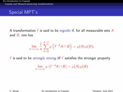
A transformation f is said to be ergodic if, for all measurable sets Aand B , one has

limn→+∞

1n

n−1∑k=0

µ(f −kA ∩ B

)= µ(A)µ(B);

f is said to be strongly mixing iIf f satisfies the stronger property

limn→+∞

µ(f −nA ∩ B

)= µ(A)µ(B)



Two corollaries

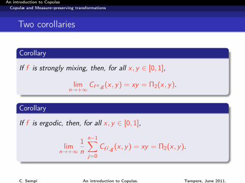
Corollary

If f is strongly mixing, then, for all x , y ∈ [0, 1],

limn→+∞

Cf n,g (x , y) = xy = Π2(x , y).

Corollary

If f is ergodic, then, for all x , y ∈ [0, 1],

limn→+∞

1n

n−1∑j=0

Cf j ,g (x , y) = xy = Π2(x , y).



Two examples

For the copula M2 one has

λ(f −1 [0, x ] ∩ f −1 [0, y ]

)= λ

(f −1 ([0, x ] ∩ [0, y ])

)= λ ([0, x ] ∩ [0, y ]) = minx , y = M2(x , y).

for every measure–preserving transformation f .As for the copula W2, recall that it concentrates all the probabilitymass uniformly on the the diagonal ϕ(t) = 1− t of the unit square.In this case ϕ = ϕ−1, so that

λ(ϕ−1 [0, x ] ∩ [0, y ]

)= λ ([1− x , 1] ∩ [0, y ])

=

0, if x ≤ 1− y ,x + y − 1, if x > 1− y ;

thereforeW2(x , y) = λ

(ϕ−1 [0, x ] ∩ [0, y ]

).



The independence copula

TheoremLet f and g be measure–preserving transformations. The followingconditions are equivalent for Cf ,g ∈ C2:(a) Cf ,g = Π2

(b) f and g, when regarded as random variables on the standardprobability space (I,B(I), λ), are independent.


An introduction to CopulasConstruction of copulas

Patchwork

An at most countable family (Si )i∈I of closed and connectedsubsets of I2

Si ∩ Sj ⊂ ∂Si ∩ ∂Sj

C – a copulaa continuous function Fi : Si → I2 that is isotone in each placeand agrees with C (called background) on the the boundary∂Si of Si , namely Fi (u, v) = C (u, v) for every (u, v) ∈ ∂Si

The function F : I2 → I

F (u, v) :=

Fi (u, v) , (u, v) ∈ Si ,

C (u, v) , elsewhere,

is called the patchwork of (Fi )i∈I into C .C. Sempi An introduction to Copulas. Tampere, June 2011.


Patchwork copulæ

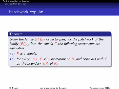
TheoremGiven the family (Ri )i∈I of rectangles, for the patchwork of thefamily (Fi )i∈I into the copula C the following statements areequivalent:(a) F is a copula;(b) for every i ∈ I , Fi is 2–increasing on Ri and coincides with C

on the boundary ∂Ri of Ri .



Ordinal sums

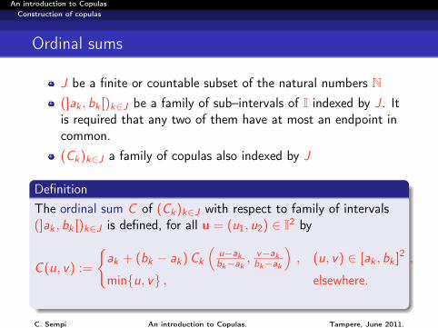
J be a finite or countable subset of the natural numbers N(]ak , bk [)k∈J be a family of sub–intervals of I indexed by J. Itis required that any two of them have at most an endpoint incommon.(Ck)k∈J a family of copulas also indexed by J

DefinitionThe ordinal sum C of (Ck)k∈J with respect to family of intervals(]ak , bk [)k∈J is defined, for all u = (u1, u2) ∈ I2 by

C (u, v) :=

ak + (bk − ak)Ck

(u−akbk−ak

, v−akbk−ak

), (u, v) ∈ [ak , bk ]2 ,

minu, v , elsewhere.



Ordinal sums–2

TheoremThe ordinal sum of the family of copulas (Ck)k∈J with respect tothe family of intervals (]ak , bk [)k∈J is a copula.

An ordinal sum is a special case of the construction of patchworkcopulas; it suffices to choose

the copula M2 as the background copula;Sk = ]ak , bk [× ]ak , bk [ for every k ∈ J;for every k ∈ J, Fk is a version of the copula Ck rescaled insuch a way as to meet the requirements of a patchwork



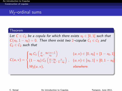
W2–ordinal sums

TheoremLet C ∈ C2 be a copula for which there exists x0 ∈ ]0, 1[ such thatC (x0, 1− x0) = 0. Then there exist two 2–copulæ C1 ∈ C2 andC2 ∈ C2 such that

C (u, v) =

x0 C1

(ux0 ,

x0+v−1x0

)(u, v) ∈ [0, x0]× [1− x0, 1]

(1− x0)C2

(u−x01−x0 ,

v1−x0

), (u, v) ∈ [x0, 1]× [0, 1− x0]

W2(u, v), elsewhere.


An introduction to CopulasShuffles of Min

Shuffles of Min

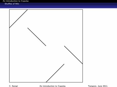
A copula is said to be a shuffle of Min it is obtained through thefollowing procedure:

the probability mass is placed on the support of the copulaM2, namely on the main diagonal of the unit square;then the unit square is cut into a finite number of verticalstrips;these vertical strips are permuted (“shuffled”) and, possibly,some of them are flipped about their vertical axes of symmetry;finally the vertical strips are reassembled to form the unitsquare again;to the probability mass thus obtained there corresponds aunique copula C , which is a shuffle of Min.

Shuffles of Min were introduced in (Mikusiński et al. (1992)).





A different presentation

Two continuous random variables X and Y have a shuffle of Min Cas their copula is if, and only if, one of them is an invertiblepiecewise linear function of the other one.

The set of Shuffles of Min is dense in C2.



Density of the shuffles

TheoremLet X and Y be continuous random variables on the sameprobability space (Ω,F ,P), let F and G be their marginal d.f.’s andH their joint d.f.. Then, for every ε > 0 there exist two randomvariables Xε and Yε on the same probability space and a piecewiselinear function ϕ : R→ R such that(a) Yε = ϕ Xε(b) Fε := FXε = F and Gε := FYε = G(c) ‖H − Hε‖∞ < ε

where Hε is the joint d.f. of Xε and Yε, and ‖ · ‖∞ denotes theL∞–norm on R2.



A surprising consequence

The last result has a surprising consequence. Let X and Y beindependent (and continuous) random variables on the sameprobability space, let F and G be their marginal d.f.’s andH = F ⊗ G their joint d.f.. Then, according to the previoustheorem, it is possible to construct two sequences (Xn) and (Yn) ofrandom variables such that, for every n ∈ N, their joint d.f. Hnapproximates H to within 1/n in the L∞–norm, but Yn is almostsurely a (piecewise linear) function of Xn.



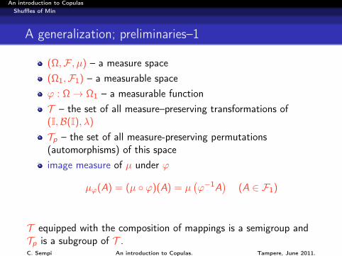
A generalization; preliminaries–1

(Ω,F , µ) – a measure space(Ω1,F1) – a measurable spaceϕ : Ω→ Ω1 – a measurable functionT – the set of all measure–preserving transformations of(I,B(I), λ)

Tp – the set of all measure-preserving permutations(automorphisms) of this spaceimage measure of µ under ϕ

µϕ(A) = (µ ϕ)(A) = µ(ϕ−1A

)(A ∈ F1)

T equipped with the composition of mappings is a semigroup andTp is a subgroup of T .C. Sempi An introduction to Copulas. Tampere, June 2011.


Interval exchange transformations

J1,i (i = 1, 2, . . . , n) – partition of I into the non–degenerateintervals J1,i = [a1,i , b1,i [ and the singleton J1,n = 1.J2,i (i = 1, 2, . . . , n) – another such partition such that,λ(J1,i ) = λ(J2,i )the interval exchange transformation

T (x) =

x − a1,1 + a2,1, if x ∈ J1,i ,λ ((I \

⋃ni=1 J1,i ) ∩ [0, x ]) +

∑ni=1(b2,i − a2,a) 1[a2,1](x)

otherwise,



A mapping on I2

Given T : I→ I define ST : I2 → I2 via

ST (u, v) := (T (u), v) . ((u, v) ∈ I2)

J – a (possibly degenerate) interval in Ithe (vertical) strip J × Ithe partition of the unit square I2 into possibly infinitely many,vertical strips.



Generalized shuffling

A shuffling of a strip partition Ji × Ii∈I (card I ≤ ℵ0) is anypermutation S of the unit square such that

(1Sh) admits the representation S = ST for some T : I→ I(2Sh) is measure–preserving on the space

(I2,B(I2), λ2

)(3Sh) the restriction S |Ji×I of S to every strip Ji × I is continuous

with respect to the standard product topology on I2



Generalized shuffling–2

Intuitively, shuffling is just a reordering of the strips. This feature iscaptured by the condition (1Sh), which represents the shuffling by asingle transformation T of the unit interval. In particular, ST is apermutation of I2 if, and only if, T is a permutation of I. Becauseof (2Sh) the single strips maintain their measure after shuffling.Finally, condition (3Sh) is just a technical tool for ensuring that,during shuffling, the integrity of strips is preserved.



Shuffles: the new characterization

LemmaConsider the image measure of a doubly stochastic measure µunder ST . Then the following statements are equivalent:(a) µST is doubly stochastic(b) T is in T .

TheoremThe following statements are equivalent:(a) a copula C ∈ C2 is a shuffle of Min;(b) there exists a piece–wise continuous T ∈ T such that

µC = µM2 S−1T



Shuffles: the new definition

Definition

A copula C ∈ C2 is a generalized shuffle of Min if µC = µM2 S−1T

for some T ∈ T . Such a shuffle of Min is denoted by MT .

In this definition, T is allowed to have countably manydiscontinuity points, which is a quite natural generalization of theoriginal notion of shuffle of Min.



Shuffling an arbitrary copula

DefinitionLet C ∈ C2 be a copula. A copula A is a shuffle of C if there existsT ∈ T such that µA = µC S−1T . In this case, A is also called theT–shuffle of C and denoted by CT .

If a copula C is represented by means of two measure–preservingtransformations f and g , Cf ,g , then

(Cf ,g )T = CTf ,g



Orbits

The mapping which assigns to every T ∈ T and to every copulaC ∈ C2 the corresponding shuffle CT defines an action of the groupT on the set of all copulas. The orbit of a copula C with respect tothis action is the set T (C ) = CT | T ∈ T constituted by allshuffles of C . The general theory of group actions guarantees thatthe classes of type T (C ) form a partition of the set of all copulas.The orbit of a copula is exactly the collection of all its shuffles.

TheoremFor a copula C ∈ C2 the following statements are equivalent:(a) C = Π2;(b) T (C ) = C.



More on shuffles

TheoremIf C ∈ C2 is absolutely continuous then so are all its shuffles.

TheoremEvery copula C ∈ C2 other than Π2 has a non–exchangeable shuffle.

TheoremFor every copula C ∈ C2, the independence copula Π2 can beapproximated uniformly by elements of T (C ).


An introduction to CopulasArchimedean copulæ

Generators

A function ϕ : R+ → I is said to be an (outer additive) generator ifit is continuous, decreasing and ϕ(0) = 1, limt→+∞ ϕ(t) = 0 and isstrictly decreasing on [0, t0], where t0 := inft > 0 : ϕ(t) = 0. Ifthe function ϕ is invertible, or, equivalently, strictly decreasing onR+, then the generator is said to be strict. If ϕ is strict, thenϕ(t) > 0 for every t > 0 (and limt→+∞ ϕ(t) = 0).



Archimedan copulæ

A copula C ∈ Cd is said to be Achimedean if a generator ϕ existssuch that

C (u) = ϕ(ϕ(−1)(u1) + ϕ(−1)(u2) + · · ·+ ϕ(−1)(ud )

)u ∈ Id .

Such a copula will be denoted by CϕWhen ϕ is strict the copula Cϕ is said to be strict; in this case, Cϕhas the representation

Cϕ(u) = ϕ(ϕ−1(u1) + · · ·+ ϕ−1(ud )

).



d–monotone functions

A function f : ]a, b[→ R is called d–monotone in ]a, b[, where−∞ ≤ a < b ≤ +∞ if

it is differentiable up to order d − 2;for every x ∈ ]a, b[, its derivatives satisfy the inequalities

(−1)k f (k)(x) ≥ 0, (k = 0, 1, . . . , d − 2)

(−1)d−2 f (d−2) is decreasing and convex in ]a, b[

f is 2–monotone function iff it is decreasing and convex. If f hasderivatives of every order and if

(−1)k f (k)(x) ≥ 0,

for every x ∈ ]a, b[ and for every k ∈ Z+ is said to be completelymonotonic.C. Sempi An introduction to Copulas. Tampere, June 2011.


Characterization of Archimedean copulas

Theorem(McNeil & Nešlehová) Let ϕ : R+ → I be a generator. Then thefollowing statements are equivalent:(a) ϕ is d–monotone on ]0,+∞[;(b) Cϕ(u) := ϕ

(ϕ(−1)(u1) + · · ·+ ϕ(−1)(ud )

)is a d–copula.

CorollaryLet ϕ : R+ → I be a generator. Then the following statements areequivalent:(a) ϕ is completely monotone on ]0,+∞[

(b) Cϕ : Id → I is a d–copula for every d ≥ 2



Examples

The copula Π2 is Archimedean: take ϕ(t) = e−t ; sincelimt→+∞ ϕ(t) = 0 and ϕ(t) > 0 for every t > 0, ϕ is strict; thenϕ−1(t) = − ln t and

ϕ(ϕ−1(u) + ϕ−1(v)

)= exp (− (− ln u − ln v)) = uv = Π2(u, v).

Also W2 is Archimedean; take ϕ(t) := max1− t, 0. Sinceϕ(1) = 0, ϕ is not strict. Its quasi–inverse is ϕ(−1)(t) = 1− t.On the contrary, the upper Fréchet–Hoeffding bound M2 is notArchimedean.



The Gumbel–Hougaard family

CGHθ (u) = exp

−( d∑i=1

(− log(ui ))θ

)1/θwhere θ ≥ 1. For θ = 1 we obtain the independence copula as aspecial case, and the limit of CGH

θ for θ → +∞ is thecomonotonicity copula. The Archimedean generator of this familyis given by ϕ(t) = exp

(−t1/θ

). Each member of this class is

absolutely continuous.



The Mardia–Takahasi–Clayton family

The standard expression for members of this family of d–copulas is

CMTCθ (u, v) = max

(

d∑i=1

u−θi − (d − 1)

)−1/θ, 0

where θ ≥ −1

d−1 , θ 6= 0. The limiting case θ = 0 corresponds to theindependence copula.The Archimedean generator of this family is given by

ϕθ(t) = (max1 + θt, 0)−1/θ .

For every d–dimensional Archimedean copula C and for everyu ∈ Id , CθθLu ≤ C (u) for θL = − 1

d−1 .



Frank’s family

CFrθ (u) = −1

θlog

(1 +

∏di=1(e−θui − 1

)(e−θ = 1)

d−1

),

where θ > 0. The limiting case θ = 0 corresponds to Πd . For thecase d = 2, the parameter θ can be extended also to the caseθ < 0.Copulas of this type have been introduced by Frank in relation witha problem about associative functions on I. They are absolutelycontinuous.The Archimedean generator is given by

ϕθ(t) = −1θ log

(1− (1− e−θ) e−t

)



EFGM copulæ–1

For d ≥ 2 let S be the class of all subsets of 1, 2, . . . , d havingat least 2 elements; S contains 2d − d − 1 elements. To eachS ∈ S, we associate a real number αS , with the convention that,when S = i1, i2, . . . , ik, αS = αi1i2...ik .An EFGM copula can be expressed in the following form:

CEFGMd (u) =

d∏i=1

ui

1 +∑S∈S

αS∏j∈S

(1− uj)

,

for suitable values of the αS ’s.For the bivariate case EFGM copulæ have the following expression:

CEFGM2 u1, u2 = u1u2 (1 + α12(1− u1)(1− u2)) ,



EFGM copulæ–2

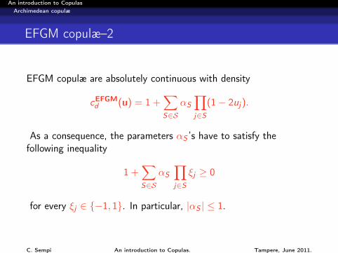
EFGM copulæ are absolutely continuous with density

cEFGMd (u) = 1 +

∑S∈S

αS∏j∈S

(1− 2uj).

As a consequence, the parameters αS ’s have to satisfy thefollowing inequality

1 +∑S∈S

αS∏j∈S

ξj ≥ 0

for every ξj ∈ −1, 1. In particular, |αS | ≤ 1.


An introduction to CopulasHow many Archimedean copulæ are there?

A necessary detour: associativity

DefinitionA binary operation T on I is said to be associative if, for all s, tand u in I,

T (T (s, t), u) = T (s,T (t, u))

DefinitionThe T–powers of an element t ∈ I under the associative functionT are defined recursively by

t1 := t and ∀n ∈ N tn+1 := T (tn, t) ,



t–norms

Definition

A triangular norm, or, briefly, a t–norm T is a function T : I2 → Ithat is associative, commutative, isotone in each place, viz., boththe functions

I 3 t 7→ T (t, s) and I 3 t 7→ T (s, t)

are isotone for every s ∈ I and such that T (1, t) = t for everyt ∈ I.

DefinitionA t–norm T is said to be Archimedean if, for all s and t in ]0, 1[,there is n ∈ N such that sn < t.



Copulæ and t–norms

TheoremFor a t–norm T the following statements are equivalent:(a) T is a 2–copula;(b) T satisfies the Lipschitz condition:

T (x ′, y)− T (x , y) ≤ x ′ − x x , x ′, y ∈ I x ≤ x ′

TheoremFor an Archimedean t–norm T, which has ϕ as an outer additivegenerator, the following statements are equivalent:(a) T is a 2–copula;(b) either ϕ or ϕ(−1) is convex.



Two important concepts

DefinitionAn element a ∈ ]0, 1[ is said to be a nilpotent element of thet–norm T if there exists n ∈ N such that a(n)

T = 0.

Definition

A t–norm T is said to be strict if it is continuous on I2 and isstrictly increasing on ]0, 1[; it is said to be nilpotent if it iscontinuous on I2 and every a ∈ ]0, 1[ is nilpotent.

The t–norm Π2(u, v) := uv is strict, whileW2(u, v) := maxu + v − 1, 0 is nilpotent.

∀ a ∈ ]0, 1[ anW2

= maxna − (n − 1), 0,

so that anW2

= 0 for n ≥ 1/(1− a).



Representation of t–norms

Under mild conditions the t–norm T has the followingrepresentation

T (x , y) = ϕ(ϕ(−1)(x) + ϕ(−1)(y)

)x , y ∈ I,

where ϕ : R+ → I is continuous, decreasing and ϕ(0) = 1, whileϕ(−1) : I→ R+ is a quasi–inverse of ϕ that is continuous, strictlydecreasing on I and such that ϕ(−1)(1) = 0



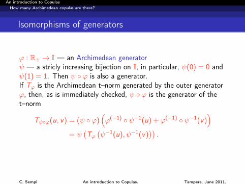
Isomorphisms of generators

ϕ : R+ → I — an Archimedean generatorψ — a stricly increasing bijection on I, in particular, ψ(0) = 0 andψ(1) = 1. Then ψ ϕ is also a generator.If Tϕ is the Archimedean t–norm generated by the outer generatorϕ, then, as is immediately checked, ψ ϕ is the generator of thet–norm

Tψϕ(u, v) = (ψ ϕ)(ϕ(−1) ψ−1(u) + ϕ(−1) ψ−1(v)

)= ψ

(Tϕ(ψ−1(u), ψ−1(v)

)).



Isomorphisms of generators–2

DefinitionTwo generators ϕ1 and ϕ2 are said to be isomorphic if there existsa strictly increasing bijection ψ : I→ I such that ϕ2 = ψ ϕ1.Two t–norms T1 and T2 are said to be isomorphic if there exists astrictly increasing bijection ψ : I→ I such that, for all u and v in I,

T2(u, v) = ψ(T1(ψ−1(u), ψ−1(v)

)).



Two results on t–norms

Theorem

For a function T : I2 → I, the following statements are equivalent:(a) T is a strict t–norm;(b) T is isomorphic to Π2.

Theorem

For a function T : I2 → I, the following statements are equivalent:(a) T is a nilpotent t–norm;(b) T is isomorphic to W2.



Isomorphisms for copulas–1

TheoremFor an Archimedean 2–copula C ∈ C2, the following statements areequivalent:(a) C is strict;(b) C is isomorphic to Π2;(c) every additive generator ϕ of C is isomorphic to ϕΠ2(t) = e−t

(t ∈ R+)



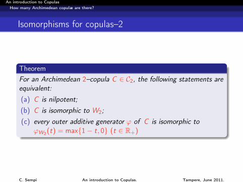
Isomorphisms for copulas–2

TheoremFor an Archimedean 2–copula C ∈ C2, the following statements areequivalent:(a) C is nilpotent;(b) C is isomorphic to W2;(c) every outer additive generator ϕ of C is isomorphic to

ϕW2(t) = max1− t, 0 (t ∈ R+)



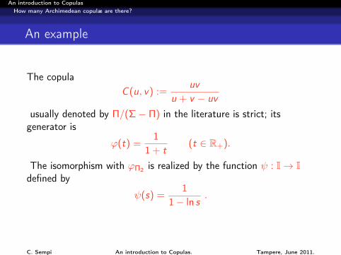
An example

The copulaC (u, v) :=

uvu + v − uv

usually denoted by Π/(Σ− Π) in the literature is strict; itsgenerator is

ϕ(t) =1

1 + t(t ∈ R+).

The isomorphism with ϕΠ2 is realized by the function ψ : I→ Idefined by

ψ(s) =1

1− ln s.


An introduction to CopulasCopulæ and Brownian motion

Brownian motion

In a probability space (Ω,F ,P) let B(1)t : t ≥ 0 and

B(2)t : t ≥ 0 be two Brownian motions (=BM’s). We explicitly

assume that the BM is continuous and consider, for every t ≥ 0,the random vector

Bt :=(B(1)

t ,B(2)t

)Then Bt : t ≥ 0 defines a stochastic process with values in R2.The literature deals mainly with the independent case, viz., B(1)

t

and B(2)t are independent for every t ≥ 0; this is usually called the

two–dimensional BM.



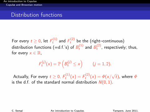
Distribution functions

For every t ≥ 0, let F (1)t and F (2)

t be the (right–continuous)distribution functions (=d.f.’s) of B(1)

t and B(2)t , respectively; thus,

for every x ∈ R,

F (j)t (x) = P

(B(j)

t ≤ x)

(j = 1, 2).

Actually, For every t ≥ 0, F (1)t (x) = F (2)

t (x) = Φ(x/√t), where Φ

is the d.f. of the standard normal distribution N(0, 1).



Coupled BM–1

For every t ≥ 0, let Ct , which depends on t, be the bivariate copulaof the random pair (B(1)

t ,B(2)t ). Then the d.f. Ht : R2 → I of the

random pair Bt , is given, for all x and y in R, by

Ht(x , y) = Ct

(F (1)

t (x),F (2)t (y)

).

Since both B(1)t and B(2)

t are normally distributed the copula Ct isuniquely determined for every t ≥ 0.



Coupled BM–2

Through an abuse of notation we shall write

Bt := Ct

(B(1)

t ,B(2)t

)Notice that, in principle, a different copula is allowed for everyt ≥ 0. The process Bt : t ≥ 0 will be called the 2–dimensionalcoupled Brownian motion.The traditional two–dimensional BM is included in the picture; inorder to recover it, it suffices to choose the independence copulaΠ2(u, v) := u v ((u, v) ∈ I2) and set Ct = Π2 for every t ≥ 0

Ht(x , y) = F (1)t (x)F (2)

t (y) ((x , y) ∈ R2).



Properties to be studied

The (one–dimensional) BM is the example of a stochastic processthat has three properties

it a Markov process;it is a martingale in continuous time;it is a Gaussian process.

These three aspects will be examined for a coupled BM.



The Markov property

Since the Markov property for a d–dimensional processXt : t ≥ 0 disregards the dependence relationship of itscomponents at every t ≥ 0, but is solely concerned with thedependence structure of the random vector Xt at different times,the traditional proof for the ordinary (independent) BM holds forthe coupled BM Bt := Ct(B(1)

t ,B(2)t ) : t ≥ 0. Therefore,

Theorem

A coupled Brownian motion Bt := Ct(B(1)t ,B(2)

t ) : t ≥ 0 is aMarkov process.



The coupled BM is a martingale

Theorem

The coupled Brownian motion Bt := Ct(B(1)t ,B(2)

t ) : t ≥ 0 is amartingale.



Gaussian processes

One has first to state what is meant by the expression Gaussianprocess when a stochastic process with values in R2 is considered.We shall adopt the following definition.

Definition

A stochastic process Xt : t ≥ 0 with values in Rd is said to beGaussian if, for every n ∈ N, and for every choice of n times0 ≤ t1 < t2 < · · · < tn, the random vector (Xt1 ,Xt2 , . . . ,Xtn) has a(d × n)–dimensional normal distribution.



Is a coupled BM a Gaussian process?

Let the copula Ct coincide, for every t ≥ 0, with M2, i.e.,M2(u, v) = minu, v, u and v in I. Then

Ht(x , y)

=1√2π t

min∫ x

−∞exp−v2/(2t) du,

∫ y

−∞exp−u2/(2t) dv

= Φ

(minx , y√

t

).

A simple calculation shows that

∂2Ht(x , y)

∂x ∂y= 0 a.e.

with respect to the Lebesgue measure λ2, so that Ht is not evenabsolutely continuous.C. Sempi An introduction to Copulas. Tampere, June 2011.


Example–2

If the copula Ct is given, for every t ≥ 0, by W2, where

W2(u, v) := maxu + v − 1, 0,

then the d.f. Ht of Bt is given by

Ht(x , y) = maxΦ

(x√t

)+ Φ

(y√t

)− 1, 0

,

which again leads, after simple calculations, to the conclusion that,again, Bt is not even absolutely continuous.



Singular copulæ

The two previous examples represent extreme cases; in fact, sincethe d.f.’s involved are continuous, the copula of two randomvariables is M2 if, and only if, they are comonotone, namely, eachof them is an increasing function of the other, while their copula isW2 if, and only if, they are countermonotone, namely, each of themis a decreasing function of the other. In this sense both examplesare the opposite of the independent case, which is characterized bythe copula Π2.We recall that a copula can be either absolutely continuous orsingular or, again, a mixture of the two types. In general, if thecopula C is singular, namely the d.f. of a probability measureconcentrated on a subset of zero Lebesgue measure λ2 in the unitsquare I2, then also Bt is singular.



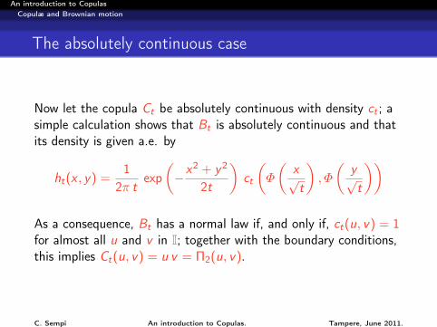
The absolutely continuous case

Now let the copula Ct be absolutely continuous with density ct ; asimple calculation shows that Bt is absolutely continuous and thatits density is given a.e. by

ht(x , y) =1

2π texp(−x2 + y2

2t

)ct

(Φ

(x√t

), Φ

(y√t

))

As a consequence, Bt has a normal law if, and only if, ct(u, v) = 1for almost all u and v in I; together with the boundary conditions,this implies Ct(u, v) = u v = Π2(u, v).



The special position of independence

Theorem

In a coupled Brownian motionBt = Ct

(B(1)

t ,B(2)t

): t ≥ 0

,

Bt has a normal law if, and only if, Ct = Π2, viz., if, and only if,its components B(1)

t and B(2)t are independent.




Carlo Sempi






Outline

1 Construction of copulas–2

2 Copulæ and stochastic processes

3 Measures of dependence

4 Quasi–copulæ


An introduction to CopulasConstruction of copulas–2

The ∗–product

DefinitionGiven two copulas A and B in C2, define a map via

(A ∗ B)(x , y) :=

∫ 1

0D2A(x , t)D1B(t, y) dt .

TheoremFor all copulas A and B, A ∗ B is a copula, namely A ∗ B ∈ C2, or,equivalently, ∗ : C2 × C2 → C2.



The ∗–product–2

LemmaFor every pair A and B of 2–copulas, one has

TA TB = TA∗B .



Continuity in one variable

TheoremConsider a sequence (An)n∈N of copulas and a copula B. If thesequence (An) converges (uniformly) to A ∈ C, An → A then both

An ∗ B −−−−→n→+∞

A ∗ B and B ∗ An −−−−→n→+∞

B ∗ A,

in other words the ∗–product is continuous in each place withrespect to the uniform convergence of copulas.



A consequence

TheoremThe binary operation ∗ is associative, viz.A ∗ (B ∗ C ) = (A ∗ B) ∗ C, for all 2–copulas A, B, and C.

Corollary

The set of copulas endowed with the ∗–product, (C2, ∗) is asemigroup with identity.



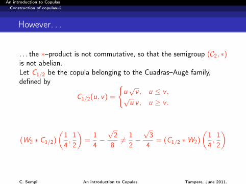
However. . .

. . . the ∗–product is not commutative, so that the semigroup (C2, ∗)is not abelian.Let C1/2 be the copula belonging to the Cuadras–Augé family,defined by

C1/2(u, v) =

u√v , u ≤ v ,

√u v , u ≥ v .

(W2 ∗ C1/2)

(14,12

)=

14−√286= 1

2−√34

= (C1/2 ∗W2)

(14,12

)



Special cases

Π2 ∗ C = C ∗ Π2 = Π2,

M2 ∗ C = C ∗M2 = C ,(W2 ∗ C )(u, v) = v − C (1− u, v),

(C ∗W2)(u, v) = u − C (u, 1− v).

In particular, one has W2 ∗W2 = M2.

TheoremThe copulæ Π2 and M2 are the (right and left) annihilator and theidentity of the ∗–product, respectively.


An introduction to CopulasCopulæ and stochastic processes

Copulæ and Conditional Expectations

TheoremLet C be the copula of the continuous random variables X and Ydefined on the probability space (Ω,F ,P); then, for almost everyω ∈ Ω,

E(1X≤x | Y

)(ω) = D2C (FX (x),FY (Y (ω)))

andE(1Y≤y | X

)(ω) = D1C (FX (X (ω)),FY (y)) .



An important consequence

CorollaryLet X , Y and Z be continuous random variables on the probabilityspace (Ω,F ,P). If X and Z are conditionally independent given Y ,then

CXZ = CXY ∗ CYZ .



∗–product and Markov processes

TheoremLet (Xt)t∈T be a real stochastic process, let each random variableXt be continuous for every t ∈ T and let Cst denote the (unique)copula of the random variables Xs and Xt (s, t ∈ T ). Then thefollowing statements are equivalent:(a) for all s, t, u in T ,

Cst = Csu ∗ Cut ;

(b) the transition probabilities P(s, x , t,A) := P (Xt ∈ A | Xs = x)satisfy the Chapman–Kolmogorov equations

P(s, x , t,A) =

∫R

P(u, ξ, t,A)P(s, x , u, dξ)

for every Borel set A, for all s and t in T with s < t, for everyu ∈ ]s, t[ ∩ T and for almost all x ∈ R.



The ?–product

The Chapman–Kolmogorov equation is a necessary but not asufficient condition for a Markov process. This motivates theintroduction of another operation on copulas.

DefinitionLet A ∈ Cm and B ∈ Cn; the ?–product of A and B is the mappingA ? B : Im+n−1 → I defined by

(A ? B)(u1, . . . , um+n−1)

:=

∫ xm

0DmA(u1, . . . , um−1, ξ)D1B(ξ, um+1, . . . , um+n−1) dξ.



Properties of the star–product

(a) for all copulas A ∈ Cm and B ∈ Cn the ?–product A ? B is an(m + n − 1)–copula, viz. ? : Cm × Cn → Cm+n−1

(b) the ?–product is continuous in each place: if the sequence(Ak)k∈N converges uniformly to A ∈ Cm, then, for everyB ∈ Cn one has both

Ak ? B −−−−→k→+∞

A ? B and B ? Ak −−−−→k→+∞

B ? A

(c) the ?–product is associative:

(A ? B) ? C = A ? (B ? C )



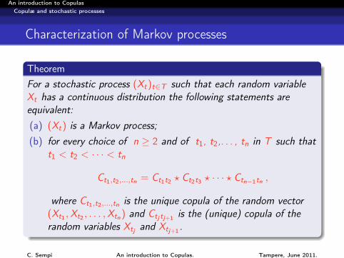
Characterization of Markov processes

TheoremFor a stochastic process (Xt)t∈T such that each random variableXt has a continuous distribution the following statements areequivalent:(a) (Xt) is a Markov process;(b) for every choice of n ≥ 2 and of t1, t2,. . . , tn in T such that

t1 < t2 < · · · < tn

Ct1,t2,...,tn = Ct1t2 ? Ct2t3 ? · · · ? Ctn−1tn ,

where Ct1,t2,...,tn is the unique copula of the random vector(Xt1 ,Xt2 , . . . ,Xtn) and Ctj tj+1 is the (unique) copula of therandom variables Xtj and Xtj+1 .



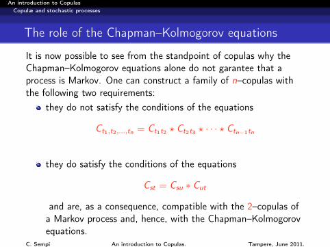
The role of the Chapman–Kolmogorov equations

It is now possible to see from the standpoint of copulas why theChapman–Kolmogorov equations alone do not garantee that aprocess is Markov. One can construct a family of n–copulas withthe following two requirements:

they do not satisfy the conditions of the equations

Ct1,t2,...,tn = Ct1t2 ? Ct2t3 ? · · · ? Ctn−1tn

they do satisfy the conditions of the equations

Cst = Csu ∗ Cut

and are, as a consequence, compatible with the 2–copulas ofa Markov process and, hence, with the Chapman–Kolmogorovequations.



Construction of the example

Consider a stochastic process (Xt) in which the random variablesare pairwise independent. Thus the copula of every pair of randomvariables Xs and Xt is given by Π2. Since, Π2 ∗ Π2 = Π2, theChapman–Kolmogorov equations are satisfied. It is now an easytask to verify that for every n > 2, the n–fold ?–product of Π2yields

(Π2 ? Π2 ? · · · ? Π2)(u1, u2, . . . , un) = Πn(u1, u2, . . . , un) ,

so that it follows that the only Markov process with pairwiseindedependent (continuous) random variables is one where all finitesubsets of random variables in the process are independent.



Construction of the example–2

On the other hand, there are many 3–copulæ whose 2–marginalscoincide with Π2; such an instance is represented by the family ofcopulas

Cα(u1, u2, u3) := Π3(u1, u2, u3)+α u1 (1−u1) u2 (1−u2) u3 (1−u3) ,

for α ∈ ]−1, 1[. Now consider a process (Xt) such thatthree of its random variables, call them X1, X2 and X3, haveCα as their copula;every finite set not containing all three of X1, X2 and X3 ismade of independent random variables;the n–copula (n > 3) of a finite set containing all three ofthem is given by

Ct1,...,tn(u1, . . . , un) = Cα(u1, u2, u3) Πn−3(u4, . . . , un) ,

where we set Π1(t) := t.C. Sempi An introduction to Copulas. Tampere, June 2011.


Construction of the example–3

Such a process exists since it is easily verified that the resultingjoint distribution satisfy the compatibility of Kolmogorov’sconsistency theorem; this ensures the existence of a stochasticprocess with the specified joint distributions. Since any two randomvariables in this process are independent, theChapman–Kolmogorov equations are satisfied. However, the copulaof X1, X2 and X3 is inconsistent with the set of equations with the?–product, so that the process is not a Markov process.



A comparison

It is instructive to compare the traditional way of specifying aMarkov process with the one due to Darsow, Olsen and Nguyen. Inthe traditional approach a Markov process is singled out byspecifying the initial distribution F0 a family of transitionprobabilities P(s, x , t,A) that satisfy the Chapman–Kolmogorovequations. Notice that in the classical approach, the transitionprobabilities are fixed, so that changing the initial distributionsimultaneously varies all the marginal distributions. In the presentapproach, a Markov process is specified by giving all the marginaldistributions and a family of 2–copulas that satisfies

Cst = Csu ∗ Cut

As a consequence, holding the copulas of the process fixed andvarying the initial distribution does not affect the other marginals.



Copulæ and Conditional expectations–2

DefinitionA copula C will be said to be idempotent (with respect to the∗–product) if

C ∗ C = C ,

or, equivalently if, for all (u, v) ∈ I2, it satisfies theintegro–differential equation

C (u, v) =

∫ 1

0D2C (u, t)D1C (t, v) dt.

Both the copulæ Π2 and M2 are idempotent.



Pfanzagl’s characterization

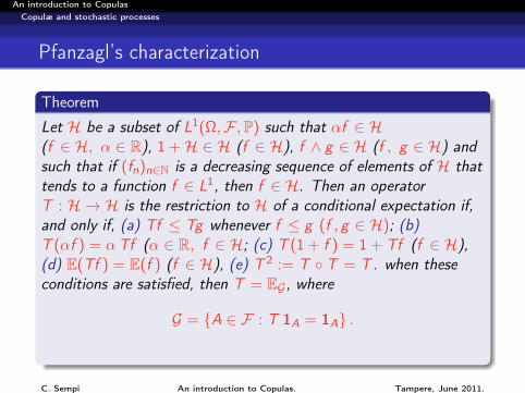
Theorem

Let H be a subset of L1(Ω,F ,P) such that αf ∈ H(f ∈ H, α ∈ R), 1 +H ∈ H (f ∈ H), f ∧ g ∈ H (f , g ∈ H) andsuch that if (fn)n∈N is a decreasing sequence of elements of H thattends to a function f ∈ L1, then f ∈ H. Then an operatorT : H → H is the restriction to H of a conditional expectation if,and only if, (a) Tf ≤ Tg whenever f ≤ g (f , g ∈ H); (b)T (αf ) = αTf (α ∈ R, f ∈ H; (c) T (1 + f ) = 1 + Tf (f ∈ H),(d) E(Tf ) = E(f ) (f ∈ H), (e) T 2 := T T = T. when theseconditions are satisfied, then T = EG , where

G = A ∈ F : T 1A = 1A .



Idempotent copulæ and Markov operators

TheoremA Markov operator T : L∞(I)→ L∞(I) is the restriction to L∞(I)of a CE if, and only if, it is idempotent, viz. T 2 = T; when thislatter condition is satisfied, then T = EG , whereG := A ∈ B(I) : T 1A = 1A.

TheoremA Markov operator T is idempotent with respect to compositionT 2 = T, if, and only if, the copula CT ∈ C2 that corresponds to itis idempotent, CT = CT ∗ CT .




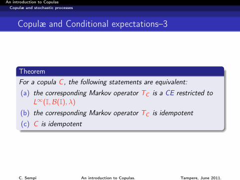
TheoremFor a copula C, the following statements are equivalent:(a) the corresponding Markov operator TC is a CE restricted to

L∞(I,B(I), λ)

(b) the corresponding Markov operator TC is idempotent(c) C is idempotent




TheoremTo every sub–σ–field G of B, the Borel σ–field of I, therecorresponds a unique idempotent copula C (G) such thatEG = TC(G). Conversely, to every idempotent copula C therecorresponds a unique sub–σ–field G(C ) of B such that TC = EG(C).

TΠ2 f = E(f ) =

∫ 1

0f (t) dt and TM2 f = f

for every f in L1(I). Therefore TΠ2 = EN , where N is the trivialσ–field ∅, I, and TM2 = EB; thus Π2 and M2 represent theextreme cases of copulas corresponding to CE’s.



Extreme copulæ

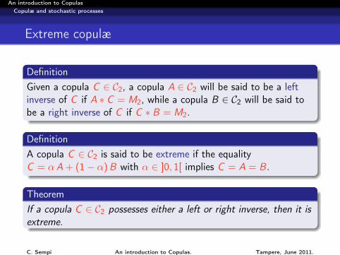
DefinitionGiven a copula C ∈ C2, a copula A ∈ C2 will be said to be a leftinverse of C if A ∗ C = M2, while a copula B ∈ C2 will be said tobe a right inverse of C if C ∗ B = M2.

DefinitionA copula C ∈ C2 is said to be extreme if the equalityC = αA + (1− α)B with α ∈ ]0, 1[ implies C = A = B .

TheoremIf a copula C ∈ C2 possesses either a left or right inverse, then it isextreme.



Inverses of copulas

TheoremWhen they exist, left and right inverses of copulas in (C2, ∗) areunique.

TheoremFor a copula C the following statements are equivalent:(a) for every v ∈ I there exists a = a(v) ∈ ]0, 1[ such that

D1C (u, v) = 1[a(v),1](u), for almost every u ∈ I;(b) C has a left inverse;(c) there exists a Borel–measurable function ϕ : R→ R such that

Y = ϕ X a.e..In either case the transpose CT of C is a left inverse of C .


An introduction to CopulasMeasures of dependence

Kendall distribution function

If X is a random variable on the probability space (Ω,F ,P) and ifits d.f. F is continuous, then the random variable F X = F (X ) isuniformly distributed on I. This is called the probability integraltransform (PIT for short)

DefinitionLet (Ω,F ,P) be a probability space and on this let X and Y berandom variables with joinf d.f. given by H and with marginals Fand G , respectively. Then the Kendall distribution function of Xand Y is the d.f. of the random variable H(X ,Y ),

KH(t) := P (H(X ,Y ) ≤ t) = µH

((x , y) ∈ R2

: H(x , y) ≤ t)

.



Kendall distribution function–2

KH depends only on the copula C of X and Y :

KC (t) := P (C (U,V ) ≤ t) = µC(

(u, v) ∈ I2 : C (u, v) ≤ t).

Consider an Archimedean copula with inner generator f ,

Cf (u, v) = g (f (u) + f (v))

thenKCf (t) = t − f (t)

f ′(t)



A characterization of Kendall d.f.

TheoremFor every copula C ∈ C2, KC is a d.f. in I such that, for every t ∈ I,(a) t ≤ KC (t) ≤ 1(b) `−KC (0) = 0Moreover the bounds of (a) are attained, since KM2(t) = t andKW2(t) = 1 for every t ∈ I.For every d.f. F that satisfies properties (a) and (b) there exists acopula C ∈ C2 for which F = KC .



Kendall’s tau

Let (X1,Y1) and (X2,Y2) be a pair of independent random vectorsdefined on (Ω,F ,P) with joint d.f. H; then the population versionof Kendall’s tau is defined as the difference of the probabilities ofconcordance and discordance, respectively, namely

τX ,Y := P [(X1 − X2) (Y1 − Y2) > 0]−P [(X1 − X2) (Y1 − Y2) < 0] .



The concordance function

TheoremLet X1, Y1, X2, Y2 be continuous random variables on theprobability space (Ω,F ,P). Let the random vectors (X1,Y1) and(X2,Y2) be independent, let H1 and H2 be their respective jointd.f.’s and let the marginals d.f.’s satisfy FX1 = FX2 = F andFY1 = FY2 = G, so that H1 and H2 both belong to the Fréchetclass Γ(F ,G ) and H1(x , y) = C1(F (x),G (y)) andH2(x , y) = C2(F (x),G (y)), where C1 and C2 are the (unique)copulæ of (X1,Y1) and (X2,Y2), respectively. Define

Q := P [(X1 − X2) (Y1 − Y2) > 0]− P [(X1 − X2) (Y1 − Y2) < 0] .

Then Q depends only on C1 and C2 and is given by

Q(C1,C2) = 4∫I2C2(s, t) dC1(s, t)− 1



Kendall’s tau and copulæ

CorollaryThe Kendall’s tau of two continuous random variables X and Y onthe probability space (Ω,F ,P) depends only on the (unique) copulaC of X and Y and is given by

τX ,Y = 4∫I2C (s, t) dC (s, t)− 1 .

In terms of the Kendall d.f.

τ(C ) = 3−∫ 1

0KC (t) dt



Examples

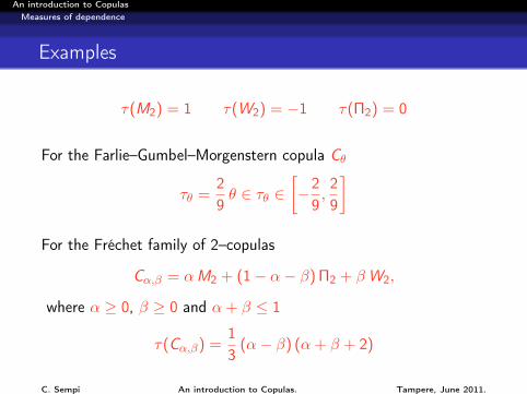
τ(M2) = 1 τ(W2) = −1 τ(Π2) = 0

For the Farlie–Gumbel–Morgenstern copula Cθ

τθ =29θ ∈ τθ ∈

[−29,29

]For the Fréchet family of 2–copulas

Cα,β = αM2 + (1− α− β) Π2 + βW2,

where α ≥ 0, β ≥ 0 and α + β ≤ 1

τ(Cα,β) =13

(α− β) (α + β + 2)



The case of Archimedean copulas

TheoremThe population version of Kendall’s tau τ(Cf ) for an Archimedeancopula Cf with inner additive generator f is given by

τ(Cf ) = 1 + 4∫ 1

0

f (t)

f ′(t)dt



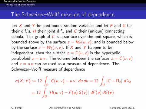
Spearman’s rho

Let (X1,Y1), (X2,Y2) and (X3,Y3) there independent continuousrandom vectors having a common joint distribution function H,with marginals F and G and copula C . Then Spearman’s rho ρXYis defined to be proportional to the difference between theprobability of concordance and the probability of discordance forthe two vectors (X1,Y1) and (X2,Y3); notice that the distributionfunction of the second vector is F ⊗ G , since X2 and Y3 areindependent. Then

ρX ,Y := 3 (P [(X1 − X2) (Y1 − Y3) > 0]− P [(X1 − X2) (Y1 − Y3) < 0])



Spearman’s rho and copulæ

TheoremIf C is the copula of two continuous random variables X and Y ,then the population version of Spearman’s rho of X and Y dependsonly on C, will be denoted indifferently by ρX ,Y or by ρC or byρ(C ), and is given by

ρX ,Y = ρC = 12∫I2u v dC (u, v)− 3 = 12

∫I2C (u, v) du dv − 3

= 12∫I2C (u, v)− u v du dv



The Schweizer–Wolff measure of dependence

Let X and Y be continuous random variables and let F and G betheir d.f.’s, H their joint d.f., and C their (unique) connectingcopula. The graph of C is a surface over the unit square, which isbounded above by the surface z = M2(u, v), and is bounded belowby the surface z = W2(u, v). If X and Y happen to beindependent, then the surface z = C (u, v) is the hyperbolicparaboloid z = u v . The volume between the surfaces z = C (u, v)and z = u v can be used as a measure of dependence. TheSchweizer–Wolff measure of dependence

σ(X ,Y ) := 12∫I2|C (u, v)− u v | du du = 12

∫I2|C − Π2| dλ2

= 12∫I2|H(u, v)− F (u)G (v)| dF (u) dG (v)



Properties of then SW measure

(SW1) σ is defined for every pair of continuous random variables Xand Y defined on the same probability space (Ω,F ,P)

(SW2) σ(X ,Y ) = σ(Y ,X )

(SW3) σ(X ,Y ) ∈ [0, 1]

(SW4) σ(X ,Y ) = 0 if, and only if, X and Y are independent;(SW5) σ(X ,Y ) = 1 if either X = ϕ Y or Y = ψ X for some

strictly monotone functions ϕ,ψ : R→ R(SW6) σ(ϕ X , ψ Y ) = σ(X ,Y ) for strictly monotone if

ϕ,ψ : R→ R(SW7) σ(X ,Y ) = 6/π arcsin(|ρ|/2) for the bivariate normal

distribution with correlation coefficient ρ(SW8) if (Xn,Yn) has joint continuous d.f. Hn and converges in law

to the random vector (X ,Y ) with continuous joint d.f. H0,then σ (Xn,Yn) −→ σ(X ,Y )



Rényi’s axioms

(R1) R is defined for any pair of random variables X and Y that arenot a.e. constant

(R2) R is symmetric, R(X ,Y ) = R(Y ,X )

(R3) for every pair of non–constant random variables X and Y ,R(X ,Y ) belongs to [0, 1]

(R4) R(X ,Y ) = 0 if, and only if, X and Y are independent(R5) R(X ,Y ) = 1 if either x = f Y or Y = g X for some Borel

measurable functions f and g(R6) if f , g : R→ R are Borel–measurable and one–to–one, then

R(f X , g Y ) = R(X ,Y )

(R7) if the joint distribution of X and Y is a bivariate normaldistribution with correlation coefficient ρ, then R(X ,Y ) = |ρ|



Other measures of dependence

the L∞ norm:

σ∞(X ,Y ) := k∞ ‖C−Π2‖∞ = k∞ sup(u,v)∈I2

|C (u, v)− Π2(u, v)| ;

the Lp norm:

σp(X ,Y ) := kp

(∫I2|C (u, v)− Π2(u, v)|p dλ2

)1/p



Measures of non–exchangeability

Let H(F ) be the class of all random pairs (X ,Y ) such that X andY are identically distributed with continuous joint d.f. F .

DefinitionA function µ : H(F )→ R+ is called a measure ofnon–exchangeability if(A1) µ is bounded, µ(X ,Y ) ≤ K(A2) µ(X ,Y ) = 0 if, and only if, (X ,Y ) is exchangeable(A3) µ is symmetric:µ(X ,Y ) = µ(Y ,X )

(A4) µ(X ,Y ) = µ(f (X ), f (Y )) for every strictly monotone functionf

(A5) if (Xn,Yn) and (X ,Y ) are pairs of random variables with jointd.f.’s Hn and H, respectively, and if Hn converges weakly to H,then µ(Xn,Yn) converges to µ(X ,Y )



In the language of copulas

Definition

A function µ : C → R+ is called a measure of non–exchangeabilityfor H(F ) if it satisfies the following properties:(B1) µ(C ) ≤ K(B2) µ(C ) = 0 if, and only if, C is symmetric;(B3) µ(C ) = µ(C t)

(B4) µ(C ) = µ(C )

(B5) if Cn −−−−→to+∞

C uniformly, then µ(Cn) −−−−→to+∞

µ(C )



An explicit measure

TheoremThe mapping µp : C → R+ defined by

µp(C ) := dp(C ,C t)

is a measure of non–exchangeability for every p ∈ [1,+∞].

TheoremFor every p ∈ [1,+∞[ and for every C ∈ C2, one has

µp(C ) ≤(

2 · 3−p

(p + 1) (p + 2)

)1/p

≤ 13.


An introduction to CopulasQuasi–copulæ

Quasi–copulæ

Definition

A track B in Id is a subset of unit cube Id that can be written inthe form

B := (F1(t),F2(t), . . . ,Fd (t)) : t ∈ I

where F1, F2, . . . , Fd are continuous d.f.’s such that Fj(0) = 0and Fj(1) = 1 for j = 1, 2, . . . , d

Definition

A d–quasi–copula is a function Q : Id → I such that for every trackB in Id there exists a d–copula CB that coincides with Q on B ,namely such that, for every point u ∈ B ,

Q(u) = CB(u).



An equivalent definition

TheoremA d–quasi–copula Q satisfies the following properties:(a) for every j ∈ 1, 2, . . . , d, Q(1, . . . , 1, uj , 1, . . . , 1) = uj

(b) Q is increasing in each place(c) Q satisfies Lipschitz condition, if u and v are in Id , then

|Q(v)− Q(u)| ≤d∑

j=1

|vj − uj |

Conversely if Q : Id → I satisfies properties (a), (b) and (b), thenit is a quasi–copula.



An immediate consequence

For d > 2 the function Wd (u) := maxu1 + · · ·+ ud − d + 1, 0 isa d–quasi–copula, but not a copula. For d > 2 consider the d–box

[1/2, 1] = [1/2, 1]× [1/2, 1]× · · · × [1/2, 1] .

Then Wd–volume of this d–box is, for d > 2,

VWd ([1/2, 1]) = 1− d2< 0,

so that Wd cannot be a copula for d > 2, but is a properquasi–copula.



A surprising result

Let µQ the real measure induced by the quasi–copula Q on(I2,B(I2)).

TheoremFor all given ε > 0 and M > 0, there exist a quasi–copula Q and aBorel subset S of I2 such that(a) µQ(S) < −M(b) for all u and v in I, |Q(u, v)− Π2(u, v)| < ε



Quasii–copulæ form a lattice

Given a set S of functions from Id into I one defines∧S(u) := infS(u) : S ∈ S.

TheoremBoth the upper and the lower bounds,

∨Q and

∧Q of every set Q

of d–quasi–copulas are quasi–copulæ,∨

Q ∈ Qd and∧

Q ∈ Qd .

Corollary

Both the upper and the lower bounds,∨

C and∧

C of every set Cof d–copulas are d–quasi–copulæ,

∨C ∈ Qd and

∧C ∈ Qd .



An example

For θ ∈ I consider the copula

Cθ(s, t) =

mins, t − θ, (s, t) ∈ [0, 1− θ]× [θ, 1] ,

mins + θ − 1, t, (s, t) ∈ [1− θ, 1]× [0, θ] ,

W2(s, t), elsewhere,

If U and V are uniform rv’s with V = U + θ (mod 1); then Cθ istheir copula. Set C =

C1/3,C2/3

, then

∨C is given by

∨C(s, t) =

max0, s − 1/3, t − 1/3, s + t − 1, −1/3 ≤ t − s ≤ 2/3,W2(s, t), elsewhere.

NoticeV∨

C

([1/3, 2/3]2

)= −1/3 < 0



Qd as a lattice

A partially ordered set P 6= ∅ is said to be a lattice if both the joinx ∨ y and x ∧ y of every pair x and y of elements of P are in P . Alattice P is said to be complete if both ∨S and ∧S belong to P forevery subset S of P .

TheoremThe set Qd of d–quasi–copulas is a complete lattice underpointwise suprema and infima.

TheoremNeither the family Cd of copulas nor the family Qd \ Cd of properquasi–copulas is a lattice.




Carlo Sempi






Outline

1 Construction of copulas: the geometric method

2 The compatibility problem


An introduction to CopulasConstruction of copulas: the geometric method

An example: the tent map

Choose θ in ]0, 1[ and consider the probability mass θ spread on thesegment joining the points (0, 0) and (θ, 1) and the probabilitymass 1− θ spread on the segment joining the points (θ, 1) and(1, 1). It is now easy to find the expression for the copula Cθ of theresulting probability distribution on the unit square:

Cθ(u, v) =

u, u ∈ [0, θ v ] ,

θ v , u ∈ ]θ v , 1− (1− θ) v [ ,

u + v − 1, u ∈ [1− (1− θ) v , 1] .



The diagonal of a copula

The diagonal section δC of a copula C ∈ Cd is the functionδC : I→ I, defined by δC (t) := C (t, t, . . . , t).The diagonal section has a probabilistic meaning. If U1, U2,. . . , Udare random variables defined on the same probability space(Ω,F ,P), having uniform distribution on (0, 1) and C as their(unique) copula, then

δC (t) = C (t, t, . . . , t) = P

d⋂j=1

Uj ≤ t

= P (maxU1,U2, . . . ,Ud ≤ t) = P

d∨j=1

Uj ≤ t

,

Then δC is the d.f. of the random variable maxU1,U2, . . . ,UdC. Sempi An introduction to Copulas. Tampere, June 2011.


Properties of the diagonal section

TheoremThe diagonal section δC of a copula C ∈ Cd , or of a quasi–copulaQ ∈ Qd , satisfies the following properties:(D1) δC (0) = 0 and δC (1) = 1(D2) ∀t ∈ I δC (t) ≤ t(D3) the function I 3 t → δC (t) is isotone;(D4) |δC (t ′)− δC (t)| ≤ d |t ′ − t| for all t and t ′ in I

The set of diagonals will be denoted by D



Questions

(Q.1) whether, given a diagonal δ ∈ D, there exists a copula Cwhose diagonal section δC coincides with δ, namely whetherthe class Cδ is non–empty;

(Q.2) whether there exist bounds for the family Cδ; these, if theyexist, are necessarily sharper than the Fréchet–Hoeffding ones;

(Q.3) whether these bounds, when they exist, are the best possible.



Answer to (Q.1)

Theorem

For every δ ∈ D, the function Kδ : I2 → I defined by

Kδ(u, v) := minu, v ,

δ(u) + δ(v)

2

is a copula with diagonal δ, so that Kδ belongs to Cδ; it will becalled the diagonal copula associated with δ.



The probabilistic meaning

TheoremLet X and Y be continuous random variables on the sameprobability space (Ω,F ,P), with a common d.f. F and copula C.Then the following statements are equivalent:(a) The joint d.f. of the random variables minX ,Y and

maxX ,Y is the Fréchet–Hoeffding upper bound(b) C is a diagonal copula.



More probability

LemmaFor every diagonal δ and for every symmetric copula C ∈ Cδ onehas C ≤ Kδ.

TheoremFor a diagonal δ the following statements are equivalent:(a) δ is the diagonal section of an absolutely continuous copula

C ∈ Cd(b) the set t ∈ I : δ(t) = t has Lebesgue measure 0,

λ(t ∈ I : δ(t) = t) = 0



The Bertino copula

For a given diagonal δ defined δ(t) := t − δ(t)

Theorem

For every diagonal δ ∈ D, the function Bδ : I2 → I defined by

Bδ(u, v) := minu, v −minδ(t) : t ∈ [u ∧ v , u ∨ v ]

=

u −mint∈[u,v ]t − δ(t), u ≤ v ,v −mint∈[v ,u]t − δ(t), v ≤ u

is a symmetric 2–copula having diagonal equal to δ, i.e., Bδ ∈ Cδ.Bδ is called the Bertino copula of δ.



Bounds for copulas with given diagonal–1

Theorem

For every diagonal δ ∈ D, the function Aδ : I2 → I defined by

Aδ(u, v) := minu, v ,maxu, v −maxδ(t) : t ∈ [u ∧ v , u ∨ v ]

=

min

u, v −maxt∈[u,v ]t − δ(t)

, u ≤ v ,

minv , u −maxt∈[v ,u]t − δ(t)

, v ≤ u

is a symmetric 2–quasi–copula having diagonal equal to δ, i.e.,Aδ ∈ Qδ.



Bounds for copulas with given diagonal–2

TheoremFor every diagonal δ and for every copula C ∈ Cδ one hasBδ ≤ C ≤ Aδ.

TheoremThe quasi–copula Aδ is a copula if, and only if, Aδ = Kδ.

TheoremFor the quasi–copula Aδ the following statements are equivalent:(a) Aδ = Kδ(b) the graph of the function t 7→ δ(t) is piecewise linear; each

segment has slope equal to 0, 1 or 2 and has at least one of itsendpoints on the diagonal v = u.


An introduction to CopulasThe compatibility problem

Statement of the problem

In its most general form, the problem runs as follows. If k and dwith 1 < k ≤ d are natural numbers, the d–copula C has

(dk

)k–marginals, which are obtained by setting d − k of its argumentsequal to 1. In the other direction, if at most

(dk

)k–copulæ are

given, there may not exist a d–copula of which the given k–copulæare the k–marginals. This may easily be seen in the case d = 3 andk = 2; if, for instance, the three two copulæ are all equal to W2,then, in view of the probabilistic meaning of the copula W2, there isno 3–copula C of which they are the marginals. On the other hand,if an d–copula exists of which the given copulæ are thek–marginals, then these are said to be compatible.



The special case d = 3 and k = 2

Let A and B be 2–copulæ, A,B ∈ C2, and denote by D(A,B) theset of all 2–copulas that are compatible with A and B , in the sensethat, if C is in D(A,B), then there exists a 3–copula C such that,for all (u, v ,w) ∈ [0, 1]3,

C (u, v , 1) = A(u, v), C (1, v ,w) = B(v ,w), C (u, 1,w) = C (u,w).

TheoremGiven any two 2–copulas A and B, there always exists a 2–copulaC that is compatible with A and B, namely D(A,B) 6= ∅, forinstance A ∗ B.



Examples

CW2,W2(u, v ,w) = max0, v + (u ∧ w)− 1,CM2,M2(u, v ,w) = u ∧ v ∧ w = M3(u, v ,w),

CW2,M2(u, v ,w) = max0, u + (v ∧ w)− 1,CM2,W2(u, v ,w) = max0, (u ∧ v)− 1 + w,

CΠ2,Π2(u, v ,w) = uvw = Π3(u, v ,w),

CΠ2,M2(u, v ,w) = u M2(v ,w),

CM2,Π2(u, v ,w) = w M2(u, v).



Properties of D(A,B)

TheoremThe set D(A,B) of copulas that are compatible with two givenbivariate copulas A and B is convex and compact with respect tothe topology of uniform convergence in I2.



Minimality of D(A,B)

The class D(A,B) is said to be minimal when D(A,B) = A ∗ B.It is worth asking: when is this the case? The following theoremprovides a sufficient condition for this to happen.

TheoremLet A and B be two bivariate copulas with A = Cf ,g and B = Cp,r ,where f , g , p and r are measure–preserving transformations from Iinto I, and either pair (f , g) or (p, r) is made of one–to–onetransformations. Then D(A,B) is minimal.

Corollary

If either A or B (or both) is a shuffle of Min, then

D(A,B) = A ∗ B.



Gluing of two copulas–1

Let A and B be d–copulæ, A,B ∈ Cd , let i ∈ 1, 2, . . . , n, andchoose θ in ]0, 1[. Define the (ui = θ)–gluing of A and B viaA

⊗ui =θ

B

(u1, . . . , ui−1, ui , ui+1, . . . , ud )

:= θA(u1, . . . , ui−1,

ui

θ, ui+1, . . . , ud

)for ui ∈ [0, θ]



Gluing of two copulas–2

A⊗ui =θ

B

(u1, . . . , ui−1, ui , ui+1, . . . , ud )

:= θA (u1, . . . , ui−1, 1, ui+1, . . . , ud )

+ (1− θ)B(u1, . . . , ui−1,

ui − θ1− θ

, ui+1, . . . , ud

)for ui ∈ [θ, 1].

TheoremFor every pair A and B of d–copulas, for every indexi ∈ 1, 2, . . . , d, and for every θ ∈ ]0, 1[, A

⊗ui =θ

B is a d–copula.


Date post:	15-May-2018
Category:	Documents
Upload:	lamhanh
View:	218 times
Download:	4 times

AnintroductiontoCopulas - Åbo...

Documents