Anisotropic Interpolation on Graphs: The Combinatorial Dirichlet Problem Leo Grady 1 and Eric L. Schwartz 2 July 21, 2003 1 L. Grady is with the Department of Cognitive and Neural Systems, Boston University, Boston, MA 02215, E-mail: [email protected]2 E. L. Schwartz is with the Departments of Cognitive and Neural Systems and Electrical and Computer Engineering, Boston University, Boston, MA 02215, E- mail: [email protected]
Transcript
Anisotropic Interpolation on Graphs: The
Combinatorial Dirichlet Problem
Leo Grady1 and Eric L. Schwartz2
July 21, 2003
1L. Grady is with the Department of Cognitive and Neural Systems, BostonUniversity, Boston, MA 02215, E-mail: [email protected]
2E. L. Schwartz is with the Departments of Cognitive and Neural Systems andElectrical and Computer Engineering, Boston University, Boston, MA 02215, E-mail: [email protected]
Abstract
The combinatorial Dirichlet problem is formulated, and an algo-rithm for solving it is presented. This provides an effective methodfor interpolating missing data on weighted graphs of arbitrary con-nectivity. Image processing examples are shown, and the relation toanisotropic diffusion is discussed.
1 Introduction
Uniformly sampled images are conventionally represented via 4-connected or8-connected (Cartesian) grids. However space-variant images require a moreflexible image topology. In previous work, the use of a graph representationhas been found to be useful for representing images whose resolution andlocal topology is not constant [1].
Space-variant sampling of visual space is ubiquitous in the higher verte-brate visual system [2]. In computer vision, this architecture is of interestbecause it facilitates real-time vision applications due to a large (albeit lossy)reduction in space-complexity [3], and because it represents a prototype foradaptive sampling in a more general setting. In a biological context, pri-mate visual sampling has been demonstrated to be strongly space variant[4], possessing a single high resolution area (fovea) with resolution falling offlinearly toward the periphery. Many non-primate species possess an evenmore exotic visual architecture. Several bird species have multiple foveas [5],and elephants have a magnified representation in the region of their trunkto facilitate “eye-trunk” coordination [6]. Computer vision systems in whichthe architecture and spatial sampling is adaptively tailored to the specificproblem domain may well follow this design path. Thus, it is of importanceto develop a universal approach to visual representation which is not implic-itly dependent on a regular Cartesian grid. Representations of image dataon graph theoretic structures provide one such route to a universal samplingand topology for visual sensing, since it separates the topological (connec-tivity) from the geometric (sampling arrangement of visual space) aspects ofthe sensor.
This paper addresses the problem of how to interpolate nodal data ona graph, and then demonstrates applications to image processing. An algo-rithm is presented that allows interpolation from known values on the nodesof a graph to missing data in such a way that the interpolated values are
1
“smooth”. The method is to solve the combinatorial Laplace equation withDirichlet boundary conditions given by the known values. A solution to thecombinatorial Laplace equation has several desirable properties in the con-text of an interpolation method (see below). Both isotropic and anisotropicinterpolation are handled similarly. Furthermore, use of the algorithm is in-dependent of the dimension in which a graph is embedded. Combinatorialdifferential operators corresponding to the vector calculus operators Div andGrad are used to develop combinatorial versions of the Laplace and Laplace-Beltrami operators. This homology between continuum and combinatorial(graph) algorithms is well known in the literature of circuit theory, mechan-ical engineering, and related areas in which discretizations of partial differ-ential equations play a central role [7]. The solution to the Laplace equationis analogous to solving an equivalent electrical circuit. The solution to prob-lems of this type, as first noted by Maxwell [8, 9], represents a minimal powerdissipation state in the electrical circuit formulation, as shown by Dirichlet’sPrinciple [10, 11]. An application of these ideas to isotropic and anisotropicimage interpolation is presented, and a brief discussion of the relation of thiswork to anisotropic diffusion is outlined.
2 Dirichlet problem
Solving the Laplace equation in order to “fill-in” missing values has been de-scribed in the context of digital elevation models [12, 13], image editing [14],and is even used by the
MATLAB function roifill.m to fill in regions ofmissing data in images. What is new about the present work is the general-ization of this interpolation concept to arbitrary geometries, topologies andmetrics, i.e., to an image representation based on an arbitrary graph ratherthan on the familiar uniform raster.
2.1 Definitions
The Dirichlet integral may be defined as
D[u] =1
2
∫
Ω
|∇u|2dΩ, (1)
for a field u and region Ω [15]. This integral arises in many physical situations,including heat transfer, electrostatics and random walks.
2
A harmonic function is a function that satisfies the Laplace equation
∇2u = 0. (2)
The problem of finding a harmonic function subject to its boundary val-ues is called the Dirichlet problem. The harmonic function that satisfiesthe boundary conditions minimizes the Dirichlet integral, since the Laplaceequation is the Euler-Lagrange equation for the Dirichlet integral [11]. In agraph setting, points for which there exist a fixed value (e.g., data nodes) aretermed boundary points. The set of boundary points provides a Dirichletboundary condition. Points for which the values are not fixed (e.g., missingdata) are termed interior points.
2.2 Interpolation
Solutions to the Laplace equation with specified boundary conditions areharmonic functions, by definition. Finding a harmonic function that satisfiesthe boundary conditions may be viewed as a method for finding values onthe interior of the volume that interpolate between the boundary values inthe “smoothest” possible fashion [15]. In this section, we discuss the proper-ties of harmonic functions that make them useful for interpolation, definingsmoothness in terms of extremal solutions to the Dirichlet integral.
From a physical standpoint, one may think of a heat source with a fixedtemperature at the center of a copper plate and a second heat source withfixed temperature on the boundary of the copper plate. The temperaturevalues taken by the plate at every point are those assumed by a harmonicfunction subject to the internal and external boundaries imposed by the heatsources. In this analogy, the temperatures measured on the inside of the cop-per plate may be viewed as smoothly interpolated between the temperatureon the internal heat source and the external heat source. The internal andexternal heat sources are considered to be boundary points, while points onthe copper plate for which temperature values are found are interior points.
Three characteristics of harmonic functions are attractive qualities forgenerating a “smooth” interpolation.
1. The mean value theorem states that the value at each point in theinterior (i.e., not a boundary point) is the average value of its neighbors[16].
3
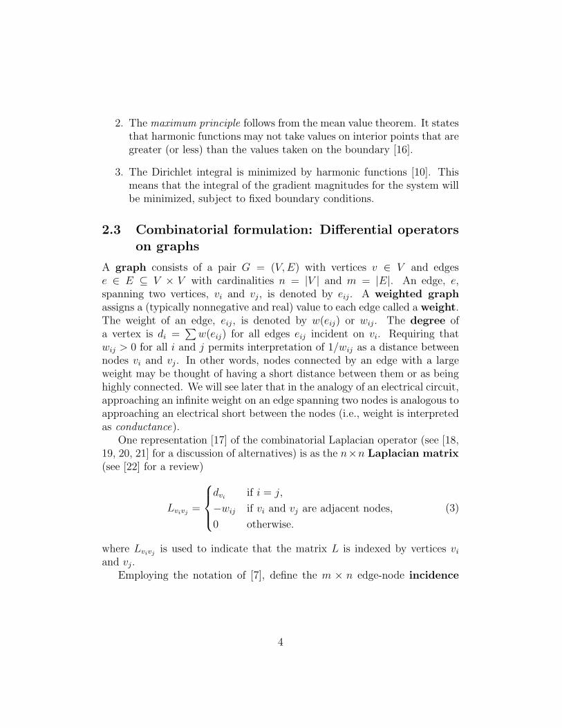
2. The maximum principle follows from the mean value theorem. It statesthat harmonic functions may not take values on interior points that aregreater (or less) than the values taken on the boundary [16].
3. The Dirichlet integral is minimized by harmonic functions [10]. Thismeans that the integral of the gradient magnitudes for the system willbe minimized, subject to fixed boundary conditions.
A graph consists of a pair G = (V,E) with vertices v ∈ V and edgese ∈ E ⊆ V × V with cardinalities n = |V | and m = |E|. An edge, e,spanning two vertices, vi and vj, is denoted by eij. A weighted graphassigns a (typically nonnegative and real) value to each edge called a weight.The weight of an edge, eij, is denoted by w(eij) or wij. The degree ofa vertex is di =
∑
w(eij) for all edges eij incident on vi. Requiring thatwij > 0 for all i and j permits interpretation of 1/wij as a distance betweennodes vi and vj. In other words, nodes connected by an edge with a largeweight may be thought of having a short distance between them or as beinghighly connected. We will see later that in the analogy of an electrical circuit,approaching an infinite weight on an edge spanning two nodes is analogous toapproaching an electrical short between the nodes (i.e., weight is interpretedas conductance).
One representation [17] of the combinatorial Laplacian operator (see [18,19, 20, 21] for a discussion of alternatives) is as the n×n Laplacian matrix(see [22] for a review)
Lvivj=
dviif i = j,
−wij if vi and vj are adjacent nodes,
0 otherwise.
(3)
where Lvivjis used to indicate that the matrix L is indexed by vertices vi
and vj.Employing the notation of [7], define the m × n edge-node incidence
4
matrix as
Aeijvk=
+1 if i = k,
−1 if j = k,
0 otherwise
(4)
for every vertex vk and edge eij, where each eij has been arbitrarily assignedan orientation. As with the Laplacian matrix above, Aeijvk
is used to indicatethat the incidence matrix is indexed by edge eij and node vk. As an operator,A may be interpreted as a combinatorial gradient operator and AT as acombinatorial divergence [23].
We define the m × m constitutive matrix, C, as the diagonal matrixwith the weights of each edge along the diagonal.
As in the continuum setting, the isotropic combinatorial Laplacian is thecomposition of the combinatorial divergence operator with the combinatorialgradient operator, L = AT A. The constitutive matrix may be interpreted asrepresenting a metric. In this sense, the combinatorial Laplacian generalizesto the combinatorial Laplace-Beltrami operator [24] via L = AT CA. Thecase of a trivial metric, (i.e., equally weighted, unit valued, edges) reduces toC = I and L = AT A.
Table 1 summarizes the relationship of familiar vector calculus operatorsto the combinatorial graph theoretic operators defined above and Table 2summarizes the relationship of equations in both domains.
With these definitions in place, we can determine how to solve for theharmonic function that interpolates values on free (“interior”) nodes betweenvalues on fixed (“boundary”) nodes.
A combinatorial formulation of the Dirichlet integral (1) is
D[u] =1
2(Au)T C(Au) =
1
2uT Lu (5)
and a combinatorial harmonic is a function u that minimizes (5). Since L ispositive semi-definite, the only critical points of D[u] will be minima.
If we want to fix the values of boundary nodes and compute the interpo-lated values across interior nodes, we may assume without loss of generalitythat the nodes in L and u are ordered such that boundary nodes are firstand interior nodes are second. Therefore, we may decompose equation (5)
5
into
D[ui] =1
2
[
uTb uT
i
]
[
Lb RRT Li
] [
ub
ui
]
= uTb Lbub + 2uT
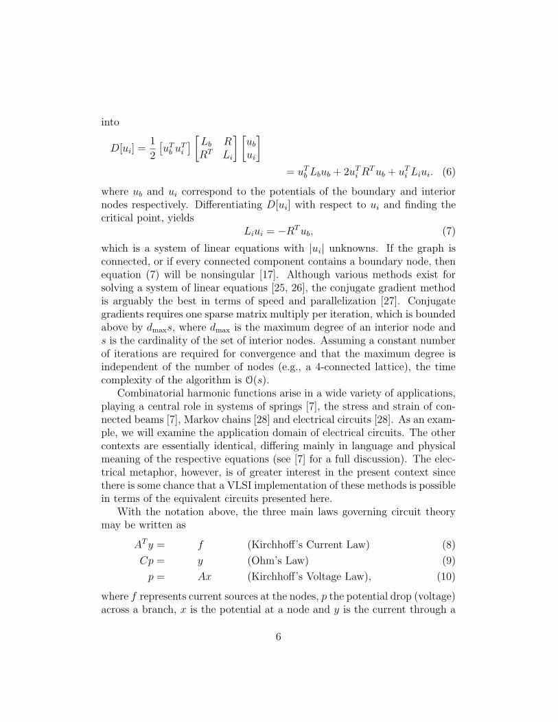
i RT ub + uTi Liui. (6)
where ub and ui correspond to the potentials of the boundary and interiornodes respectively. Differentiating D[ui] with respect to ui and finding thecritical point, yields
Liui = −RT ub, (7)
which is a system of linear equations with |ui| unknowns. If the graph isconnected, or if every connected component contains a boundary node, thenequation (7) will be nonsingular [17]. Although various methods exist forsolving a system of linear equations [25, 26], the conjugate gradient methodis arguably the best in terms of speed and parallelization [27]. Conjugategradients requires one sparse matrix multiply per iteration, which is boundedabove by dmaxs, where dmax is the maximum degree of an interior node ands is the cardinality of the set of interior nodes. Assuming a constant numberof iterations are required for convergence and that the maximum degree isindependent of the number of nodes (e.g., a 4-connected lattice), the timecomplexity of the algorithm is O(s).
Combinatorial harmonic functions arise in a wide variety of applications,playing a central role in systems of springs [7], the stress and strain of con-nected beams [7], Markov chains [28] and electrical circuits [28]. As an exam-ple, we will examine the application domain of electrical circuits. The othercontexts are essentially identical, differing mainly in language and physicalmeaning of the respective equations (see [7] for a full discussion). The elec-trical metaphor, however, is of greater interest in the present context sincethere is some chance that a VLSI implementation of these methods is possiblein terms of the equivalent circuits presented here.
With the notation above, the three main laws governing circuit theorymay be written as
AT y = f (Kirchhoff’s Current Law) (8)
Cp = y (Ohm’s Law) (9)
p = Ax (Kirchhoff’s Voltage Law), (10)
where f represents current sources at the nodes, p the potential drop (voltage)across a branch, x is the potential at a node and y is the current through a
6
Operator Vector calculus Combinatorial
Gradient ∇ A
Divergence ∇· AT
Curl ∇×∇ K
Laplacian ∇ · ∇ AT A
Beltrami ∇ C · ∇ AT CA
Table 1: Correspondence between continuum differential operators and com-binatorial differential operators on graphs. C represents a constitutive ma-trix relating flux to flow, e.g., a conductivity tensor, a diffusion tensor, athermal conductivity, a stress-strain tensor, or, in the context of differentialgeometry, a metric tensor. A is the incidence matrix of the graph represent-ing the topology of the problem. K is the cycle-edge matrix of the graph[7].
branch. The weights on a branch defining C are given by the conductanceof the branch (i.e., the reciprocal of the resistance).
The power, P , associated with a circuit may be written as
P =1
2yT C−1y =
1
2xT Lx (11)
A comparison of equations (5) and (11) demonstrates that the set of electricpotentials at the nodes of a circuit is a discrete harmonic function, i.e., thosenodes with a fixed potential due to voltage sources or grounding are theboundary nodes, the nodes without a fixed potential are the interior nodes.Furthermore, the interior nodes assume potentials that minimize (5) (see [28]for extensive discussion of electrical networks, random walks and the Dirichletintegral). If one were to build a circuit with the same topology as a graph,with appropriate voltage sources to encode the boundary values and resistorsto encode the weights, the physical solution (i.e., a minimum energy solution)to the interpolation problem would be exactly equal to the nodal potentialsof every interior node. Figure 1 illustrates the circuit corresponding to agraph interpolation problem.
7
Equation Continuum Graph
KVL ∇V = E Ax = e
KCL ∇ · J = dρ
dtAT y = f
Ohm’s Law σ−1E = J Ce = y
Dirichlet Integral 1
2
∫
Ω|∇u|2dΩ 1
2xT AT CAx
Table 2: Correspondence between continuum differential equations and com-binatorial differential equations on graphs. Kirchhoff’s current law is a quasi-static (∂B
∂t= 0) approximation to Maxwell’s Equation ∇ × E = ∂B
∂t. Kirch-
hoff’s voltage law follows from the definition of electric field as the gradientof potential. Ohm’s Law is a constitutive (phenomenological) law assertinga presumed linear dependence between voltage and current.
0
3 5
?
?
?
(a)
5V3V
− + −+
(b)
Figure 1: Interpolating on a graph with a harmonic is equivalent to settingvoltage sources (and grounds) at some nodes and reading off the potentials atnodes which are not fixed. (a) A graph with known values on some nodes andunknown values (indicated with a ‘?’) on other nodes. (b) The equivalentcircuit that would produce potentials on the nodes equal to those found bythe interpolation method.
8
3 Results
In this section we demonstrate the interpolation algorithm in the context ofimage processing.
3.1 Space-variant (foveal) images
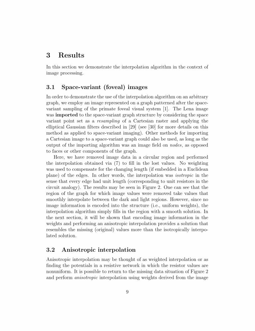
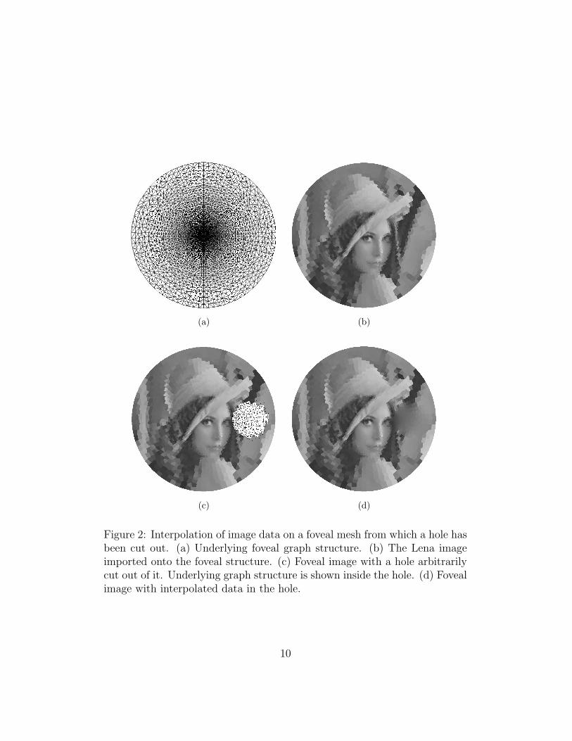
In order to demonstrate the use of the interpolation algorithm on an arbitrarygraph, we employ an image represented on a graph patterned after the space-variant sampling of the primate foveal visual system [1]. The Lena imagewas imported to the space-variant graph structure by considering the spacevariant point set as a resampling of a Cartesian raster and applying theelliptical Gaussian filters described in [29] (see [30] for more details on thismethod as applied to space-variant imaging). Other methods for importinga Cartesian image to a space-variant graph could also be used, as long as theoutput of the importing algorithm was an image field on nodes , as opposedto faces or other components of the graph.
Here, we have removed image data in a circular region and performedthe interpolation obtained via (7) to fill in the lost values. No weightingwas used to compensate for the changing length (if embedded in a Euclideanplane) of the edges. In other words, the interpolation was isotropic in thesense that every edge had unit length (corresponding to unit resistors in thecircuit analogy). The results may be seen in Figure 2. One can see that theregion of the graph for which image values were removed take values thatsmoothly interpolate between the dark and light regions. However, since noimage information is encoded into the structure (i.e., uniform weights), theinterpolation algorithm simply fills in the region with a smooth solution. Inthe next section, it will be shown that encoding image information in theweights and performing an anisotropic interpolation provides a solution thatresembles the missing (original) values more than the isotropically interpo-lated solution.
3.2 Anisotropic interpolation
Anisotropic interpolation may be thought of as weighted interpolation or asfinding the potentials in a resistive network in which the resistor values arenonuniform. It is possible to return to the missing data situation of Figure 2and perform anisotropic interpolation using weights derived from the image
9
(a) (b)
(c) (d)
Figure 2: Interpolation of image data on a foveal mesh from which a hole hasbeen cut out. (a) Underlying foveal graph structure. (b) The Lena imageimported onto the foveal structure. (c) Foveal image with a hole arbitrarilycut out of it. Underlying graph structure is shown inside the hole. (d) Fovealimage with interpolated data in the hole.
10
values (acquired before the data was removed). We employed a Gaussianweighting function [31]
wij = exp (−β|Ii − Ij|) , (12)
where Ii is the image intensity at node (pixel) i and β is a dimensionlessparameter that controls the severity of the anisotropy induced by the imageintensity. Before using equation (12) the intensity gradients were histogramequalized, since it was determined empirically that if they were not equalized,different values of the parameters would be required to produce similar resultsfor different images.
Weighting the space-variant mesh in accordance with (12) allows for amore accurate reconstruction of the missing data values, as seen in Figure 3.
Building a weighted (i.e., anisotropic) graph for an image using equation(12) allows for a smoothed reconstruction of the original image via anisotropicinterpolation from the sampling of a small number of points. These recon-structed images resemble those produced by anisotropic diffusion methods.This is because the solution to the Laplace equation is the steady state ofthe diffusion equation with specified boundary conditions [28]. The primarydifference between diffusion-based methods of image enhancement and thosepresented here is that diffusion methods approach zero (or constant) whenrun for infinite time, since Dirichlet boundary conditions are usually not spec-ified in diffusion approaches to image processing. Because of this, diffusionmethods (both isotropic and anisotropic) require a stopping condition, whilethe present method solves directly for a time-independent solution.
This relationship may be seen even more clearly by comparing the equiv-alent circuit for our interpolation algorithm and the equivalent circuit pre-sented for anisotropic diffusion by Perona and Malik [31]. If one replaced thevoltage source at every node in our circuit with an appropriately charged ca-pacitor, then the Perona-Malik equivalent circuit would be obtained exactly.Insofar as similar results are produced for image enhancement tasks with(steady state) anisotropic diffusion and the present method, two advantagesof anisotropic interpolation present themselves over diffusion. The first ofthese is that the solution to the Laplace equation is a steady state solution,while the solution to the diffusion equation depends on time. Therefore, wehave no need to iterate and, thus, we circumvent the need to choose a stop-ping point for the diffusion. Secondly, we can smooth less or smooth morein different areas of the image by decreasing the sampling density in areas
11
Figure 3: Anisotropic interpolation of image data on a foveal mesh with thesame hole as in Figure 2 has been cut out. Weights were determined usingβ = 30 (see text for details)
where we desire more smoothing and increasing it in areas where we desireless smoothing.
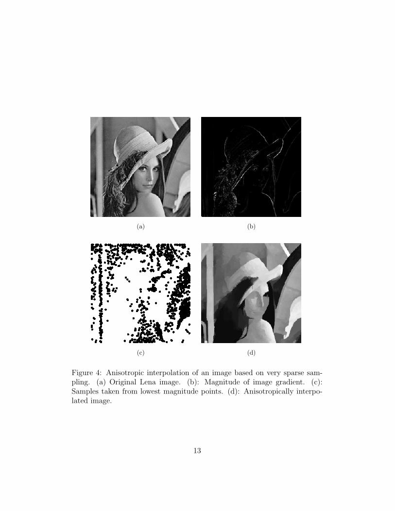
Figure 4 demonstrates results that are visually comparable to anisotropicdiffusion applied to the same image. To generate Figure 4, a 4-connectedlattice was generated with weights obtained from equation (12) based on theLena image. Samples were chosen from relatively uniform areas by computingthe square root of the sum of the edge gradients incident on each node. Allnodes with a value below a threshold were selected as sample nodes to havetheir values fixed. The remaining nodes were anisotropically interpolated,given the fixed set. One can see that sharp boundaries are maintained, dueto the encoding of image information with weights. Areas of the image withhigh variability (e.g., the feathers) are smoothed considerably since very fewsamples were taken, while areas with initially low variability remain uniform.
Of course, it is possible to interpolate by a variety of sampling strategies.Figure 5 illustrates the results of different structured sampling schemes, aswell as the flexibility to smooth more or smooth less in different areas ofthe image. Using the same weights as in Figure 4, but a different choice ofsamples, it is possible to keep the center of the image true to the originalwhile diffusing out the background or vice versa.
12
(a) (b)
(c) (d)
Figure 4: Anisotropic interpolation of an image based on very sparse sam-pling. (a) Original Lena image. (b): Magnitude of image gradient. (c):Samples taken from lowest magnitude points. (d): Anisotropically interpo-lated image.
13
Figure 5: Spatially nonuniform sampling allows for more “diffusion” in someareas over others. This figure demonstrates the effects of two different spatialsampling regimes on the anisotropic interpolation of the Lena image.
14
4 Conclusion
We have posed the question of how to interpolate nodal values on a graphand proposed a solution based on solving the combinatorial Dirichlet prob-lem. This interpolation method has desirable properties as a result of themean value theorem and the maximum principle. Furthermore, the methodnaturally incorporates a metric into the interpolation if anisotropic interpo-lation is desired. Finally, a circuit analogy was presented which both affordsadditional intuition into the process as well as holding open the possibilityfor a VLSI implementation.
Applications of this method to image processing demonstrate its usefor filling in missing values in a space-variant image and in the anisotropicsmoothing of Cartesian images. Further applications include a smoothing op-erator for multiresolution reconstruction of graph-based pyramids or three-dimensional interpolation for surfaces. Graphs are general structures thatmay arise in three dimensions for the purpose of computer graphics [32] orin an arbitrary number of dimensions for data clustering [33]. Since thisinterpolation method depends only on the topology of the structure and notany information about the dimensionality of the space in which it is embed-ded, one may interpolate on graph structures existing in arbitrary dimensionspossessing an arbitrary metric.
Acknowledgments
The authors would like to thank Jonathan Polimeni for many fruitful discus-sions and suggestions.
This work was supported in part by the Office of Naval Research (ONRN00014-01-1-0624).
References
[1] Richard Wallace, Ping-Wen Ong, and Eric Schwartz, “Space variantimage processing,” International Journal of Computer Vision, vol. 13,no. 1, pp. 71–90, Sept. 1994.
[2] Eric L. Schwartz, “Computational studies of the spatial architecture ofprimate visual cortex:columns, maps, and protomaps,” in Primary Vi-
15
sual Cortex in Primates, Alan Peters and Kathy Rocklund, Eds., vol. 10of Cerebral Cortex. Plenum Press, 1994.
[3] A. S. Rojer and E. L. Schwartz, “Design considerations for a space-variant visual sensor with complex-logarithmic geometry,” 10th Inter-
national Conference on Pattern Recognition, Vol. 2, pp. 278–285, 1990.
[4] Eric L. Schwartz, “Spatial mapping in the primate sensory projection:analytic structure and relevance to perception,” Biological Cybernetics,vol. 25, no. 4, pp. 181–194, 1977.
[5] S. P. Collin, “Behavioural ecology and retinal cell topography,” inAdaptive Mechanisms in the Ecology of Vision, S.N. Archer, M.B.A.Djamgoz, E.R. Loew, J.C. Partridge, and Dordrecht S. Vallerga, Eds.,pp. 509–535. Kluwer Academic Publishers, 1999.
[6] Jonathan Stone and Paul Halasz, “Topography of the retina in theelephant loxodonta africana,” Brain Behavior and Evolution, vol. 34,pp. 84–95, 1989.
[7] Gilbert Strang, Introduction to Applied Mathematics, Wellesley-Cambridge Press, 1986.
[8] James Clerk Maxwell, A Treatise on Electricity and Magnestism, vol. 1,Dover, New York, 3rd edition, 1991.
[9] James Clerk Maxwell, A Treatise on Electricity and Magnestism, vol. 2,Dover, New York, 3rd edition, 1991.
[10] Richard Courant, Dirichlet’s Principle, Interscience, 1950.
[11] Philip M. Morse and Herman Feshbach, Methods of Theoretical Physics,McGraw-Hill, 1953.
[12] P. A. Burrough, Principles of geographical information systems for land
resources assessment, Number 12 in Monographs on soil and resourcessurvey. Clarendon Press, Oxford, 1986.
[13] Joseph Wood and Peter Fisher, “Assessing interpolation accuracy inelevation models,” IEEE Computer Graphics and Applications, vol. 13,no. 2, pp. 48–56, March 1993.
16
[14] J. H. Elder and R. M. Goldberg, “Image editing in the contour domain,”IEEE Transactions on Pattern Analysis and Machine Intelligence, vol.23, no. 3, pp. 291–296, March 2001.
[15] R. Courant and D. Hilbert, Methods of Mathematical Physics, vol. 2 ofWiley Classics Libary, John Wiley and Sons, 1989.
[16] L. Ahlfors, Complex Analysis, McGraw-Hill, New York, 1966.
[17] Norman Biggs, Algebraic Graph Theory, Number 67 in CambridgeTracts in Mathematics. Cambridge University Press, 1974.
[18] Jozef Dodziuk, “Difference equations, isoperimetric inequality and thetransience of certain random walks,” Transactions of the American
Mathematical Soceity, vol. 284, pp. 787–794, 1984.
[19] Jozef Dodziuk and W. S Kendall, “Combinatorial laplacians and theisoperimetric inequality,” in From local times to global geometry, control
and physics, K. D. Ellworthy, Ed., vol. 150 of Pitman Research Notes in
Mathematics Series, pp. 68–74. Longman Scientific and Technical, 1986.
[20] Bojan Mohar, “Isoperimetric inequalities, growth and the spectrum ofgraphs,” Linear Algebra and its Applications, vol. 103, pp. 119–131,1988.
[21] Fan R. K. Chung, Spectral Graph Theory, Number 92 in Regional confer-ence series in mathematics. American Mathematical Society, Providence,R.I., 1997.
[22] Russell Merris, “Laplacian matrices of graphs: A survey,” Linear Alge-
bra and its Applications, vol. 197,198, pp. 143–176, 1994.
[23] Franklin H. Branin Jr., “The algebraic-topological basis for networkanalogies and the vector calculus,” in Generalized Networks, Proceed-
ings, Brooklyn, N.Y., April 1966, pp. 453–491.
[24] Frank W. Warner, Foundations of Differentiable Manifolds and Lie
Groups, Graduate Texts in Mathematics. Spring-Verlag, 1983.
[25] Gene Golub and Charles Van Loan, Matrix Computations, The JohnHopkins University Press, 3rd edition, 1996.
17
[26] Wolfgang Hackbusch, Iterative Solution of Large Sparse Systems of
Equations, Springer-Verlag, 1994.
[27] J. J. Dongarra, I. S. Duff, D. C. Sorenson, and H. A. van der Vorst, Solv-
ing Linear Systems on Vector and Shared Memory Computers, Societyfor Industrial and Applied Mathematics, Philadelphia, 1991.
[28] Peter Doyle and Laurie Snell, Random walks and electric networks,Number 22 in Carus mathematical monographs. Mathematical Associ-ation of America, Washington, D.C., 1984.
[29] Paul Heckbert, “Fundamentals of texture mapping and image warping,”M.S. thesis, University of California at Berkeley, 1989.
[30] Gen-Nan Chen, Fundamental Algorithms of Space-Variant Vision: Non-
Uniform Sampling, Triangulation, and Foveal Scale-Space, Ph.D. thesis,Boston University, 2001.
[31] Pietro Perona and Jitendra Malik, “Scale-space and edge detectionusing anisotropic diffusion,” IEEE Transactions on Pattern Analysis
and Machine Intelligence, vol. 12, no. 7, pp. 629–639, July 1990.
[32] G. Taubin, “A signal processing approach to fair surface design,” inComputer Graphics Proceedings. SIGGRAPH 95, R. Cook, Ed., LosAngeles, CA, Aug. 1995, ACM, pp. 351–358, ACM.
[33] A. K. Jain, M. N. Murty, and P. J. Flynn, “Data clustering: a review,”ACM Computing Surveys, vol. 31, no. 3, pp. 264–323, Sept. 1999.