27
Announcements • Homework 2 will be posted on the web by tonight.
| Date post: | 20-Dec-2015 |
| Category: |
Documents |
| View: | 220 times |
| Download: | 2 times |

Announcements
• Homework 2 will be posted on the web by tonight.

• Example 12.5 (Predicting the winner in election day)– Voters are asked by a certain network to participate
in an exit poll in order to predict the winner on election day.
– The exit poll consists of 765 voters. 407 say that they voted for the Republican candidate.
– The polls close at 8:00. Should the network announce at 8:01 that the Republican candidate will win?
Testing the Proportion
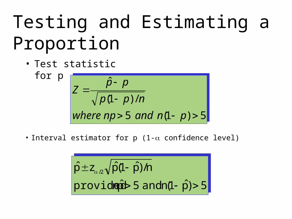
Testing and Estimating a Proportion
• Test statistic for p
• Interval estimator for p (1- confidence level)
5)1(5
/)1(
ˆ
pnandnpwhere
npp
ppZ
5)1(5
/)1(
ˆ
pnandnpwhere
npp
ppZ
5)p̂1(nand5p̂nprovided
n/)p̂1(p̂zp̂ 2/
5)p̂1(nand5p̂nprovided
n/)p̂1(p̂zp̂ 2/


Why are Proportions Different?
• The true variance of a proportion is determined by the true proportion:
• The CI of a proportion is NOT derived from the z-test:
• The denominator of the z-statistic is NOT estimated, but the width of the CI is estimated.
• => “CI test” and z-test can differ sometimes.
nppp /)1(2
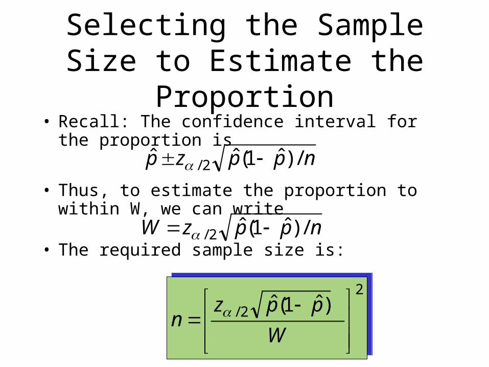
Selecting the Sample Size to Estimate the Proportion
• Recall: The confidence interval for the proportion is
• Thus, to estimate the proportion to within W, we can write
• The required sample size is:
nppzp /)ˆ1(ˆˆ 2/
nppzW /)ˆ1(ˆ2/
2
2/ )ˆ1(ˆ
W
ppzn
2
2/ )ˆ1(ˆ
W
ppzn

• Example– Suppose we want to estimate the proportion of
customers who prefer our company’s brand to within .03 with 95% confidence.
– Find the sample size needed– Solution
W = .03; 1 - = .95,
therefore /2 = .025,
so z.025 = 1.96
2
03.)p̂1(p̂96.1
n
Since the sample has not yet been taken, the sample proportionis still unknown.
We proceed using either one of the following two methods:
Sample Size to Estimate the Proportion

• Method 1:– There is no knowledge about the value of
• Let . This results in the largest possible n needed for a 1- confidence interval of the form .
• If the sample proportion does not equal .5, the actual W will be narrower than .03 with the n obtained by the formula below.
• Method 2:– There is some idea about the value of
• Use the value of to calculate the sample size
5.ˆ p03.ˆ p
p̂
068,103.
)5.1(5.96.1n
2
683
03.)2.1(2.96.1
n
2
Sample Size to Estimate the Proportion
p̂p̂
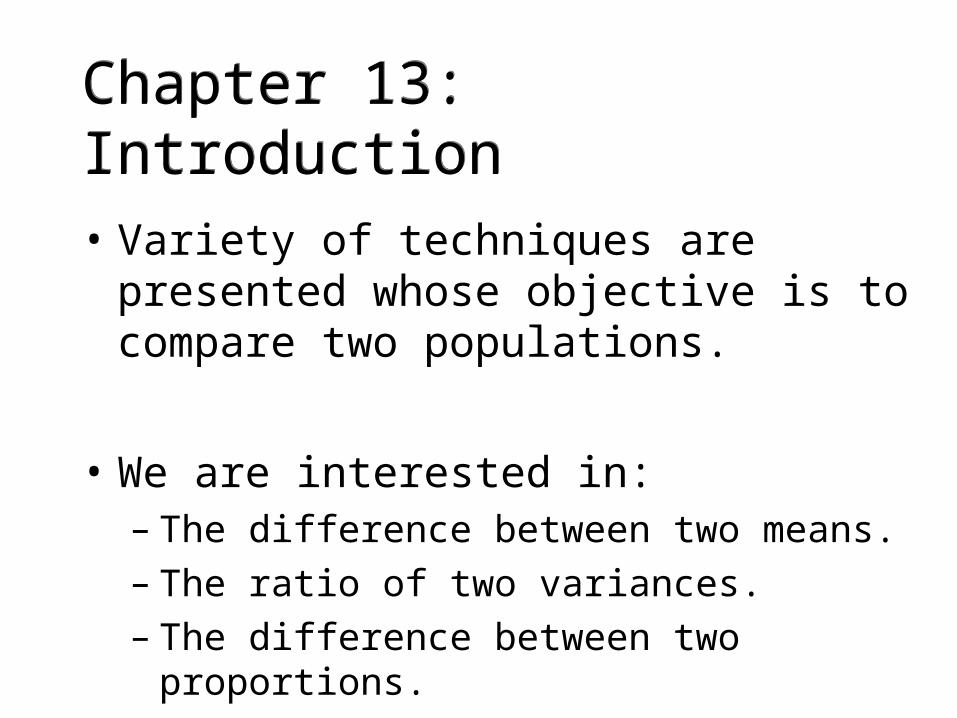
Chapter 13: IntroductionChapter 13: Introduction
• Variety of techniques are presented whose objective is to compare two populations.
• We are interested in:– The difference between two means.– The ratio of two variances.– The difference between two proportions.

Inference about the Difference between Two Means
• Example 13.1– Do people who eat high-fiber cereal for breakfast consume,
on average, fewer calories for lunch than people who do not eat high-fiber cereal for breakfast?
– A sample of 150 people was randomly drawn. Each person was identified as an eater or non-eater of high fiber cereal.
– For each person the number of calories consumed at lunch was recorded. There were 43 high-fiber eaters who had a mean of 604.02 calories for lunch with s=64.05. There were 107 non-eaters who had a mean of 633.23 calories for lunch with s=103.29.

• Two random samples are drawn from the two populations of interest.
• Because we compare two population means, we use the statistic .
13.2 Inference about the Difference between Two Means: Independent Samples
21 xx

21 xx 1. is normally distributed if the (original) population distributions are normal .
2. is approximately normally distributed if the (original) population is not normal, but the samples’ size is sufficiently large (greater than 30).
3. The expected value of is 1 - 2
4. The variance of is 12/n1 + 2
2/n2
The Sampling Distribution ofThe Sampling Distribution of
21 xx
21 xx
21 xx
21 xx

• If the sampling distribution of is normal or approximately normal we can write:
• Z can be used to build a test statistic or a confidence interval for 1 - 2
21
21
nn
)()xx(Z
21
21
nn
)()xx(Z
21xx
Making an inference about –

• Practically, the “Z” statistic is hardly used, because the population variances are not known.
? ?
• Instead, we construct a t statistic using the sample “variances” (s1
2 and s22) to estimate
Making an inference about –
21
21
ˆˆ
)()(
nn
xxt
21
21
ˆˆ
)()(
nn
xxt
22
21 ,

• Two cases are considered when producing the t-statistic:– The two unknown population variances are
equal.– The two unknown population variances are
not equal.
Making an inference about –

Inference about Inference about ––: Equal : Equal
variancesvariances
2
)1()1(
21
222
2112
nn
snsnsp
2
)1()1(
21
222
2112
nn
snsnsp
Example 1: s12 =4103.02; s2
2 = 10669.77; n1 = 43; n2 = 107.
23.8806210743
)77.10669)(1107()02.4103)(143(2
ps
• Calculate the pooled variance estimate by:
n2 = 107n1 = 43
21S
22S
The pooledvariance estimator

Inference about Inference about ––: Equal : Equal
variancesvariances• Construct the t-statistic as follows:
2nn.f.d
)n1
n1
(s
)()xx(t
21
21
2p
21
2nn.f.d
)n1
n1
(s
)()xx(t
21
21
2p
21
• Perform a hypothesis test H0: = 0 H1: > 0
or < 0 or 0
Build a confidence interval
level. confidence the is where
)n1
n1
(st)xx(21
2
p21

Example 13.1
• Assuming that the variances are equal, test the scientist’s claim that people who eat high-fiber cereal for breakfast consume, on average, fewer calories for lunch than people who do not eat high-fiber cereal for breakfast at the 5% significance level.
• There were 43 high-fiber eaters who had a mean of 604.02 calories for lunch with s=64.05. There were 107 non-eaters who had a mean of 633.23 calories for lunch with s=103.29.


1
)(
1
)(
)/(d.f.
)(
)()(
2
22
22
1
21
21
22
221
21
2
22
1
21
21
n
ns
n
ns
nsns
n
s
n
s
xxt
1
)(
1
)(
)/(d.f.
)(
)()(
2
22
22
1
21
21
22
221
21
2
22
1
21
21
n
ns
n
ns
nsns
n
s
n
s
xxt
Inference about –: Unequal variances

Inference about –: Unequal variances
Conduct a hypothesis test as needed, or, build a confidence interval
level confidence the is where
n
s
n
s2txx
intervalConfidence
)2
22
1
21()21(
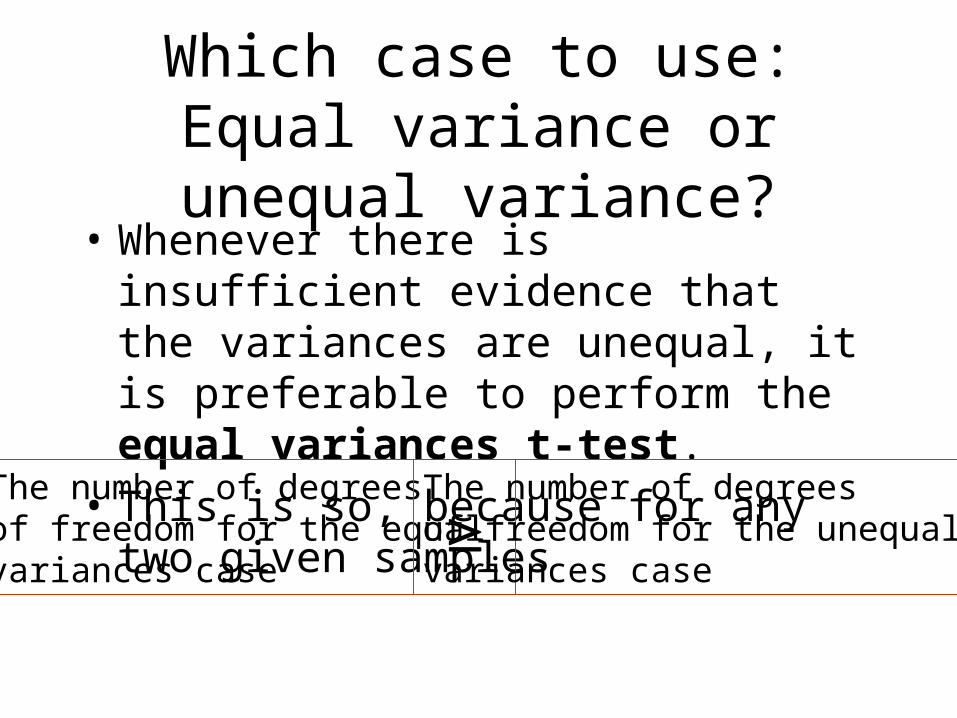
Which case to use:Equal variance or unequal
variance?• Whenever there is insufficient evidence that
the variances are unequal, it is preferable to perform the equal variances t-test.
• This is so, because for any two given samples
The number of degrees of freedom for the equal variances case
The number of degrees of freedom for the unequal variances case

Example 13.1 continued
• Test the scientist’s claim about high-fiber cereal eaters consuming less calories than non-high fiber cereal eaters assuming unequal variances at the 5% significance level.
• There were 43 high-fiber eaters who had a mean of 604.02 calories for lunch with s=64.05. There were 107 non-eaters who had a mean of 633.23 calories for lunch with s=103.29.


Tire manufacturers are constantly researching ways to produce
tires that last longer and new tires are tested by both professional
drivers and ordinary drivers on racetracks.
Suppose that to determine whether a new steel-belted radial tire
lasts longer than the company’s current model, two new-design
tires were installed on the rear wheels of 20 randomly selected cars
and two existing-design tires were installed on the rear wheels of
another 20 cars. All drivers were told to drive in their usual way
until the tires wore out. The number of miles(in 1,000s) was
recorded(Xr13-49). Can the company infer that the new tire will
last longer than the existing tire?
Additional Example-Problem 13.49Additional Example-Problem 13.49


Practice Problems
• 12.77, 12.98, 13.34,13.40


