Annual Report Graphicity and Stock Returns

Tasmanian School of Business and Economics University of Tasmania

Discussion Paper Series N 2018-08

Annual Report "Graphicity" and Stock Returns

Xiaohu Deng

University of Tasmania, Australia

Lei Gao

Iowa State University, USA

ISBN 978-1-925646-63-4

1

Annual Report “Graphicity” and Stock Returns*

Xiaohu Deng

Tasmania School of Business and Economics

University of Tasmania

Hobart, TAS 7001, Australia

[email protected]

Lei Gao

Department of Finance

Iowa State University

Ames, IA 50011, United States

[email protected]

First Draft: September 2017

This Draft: December 2018

* We would like to thank Andrea Lu, Charles Lee, Michael Sockin, Zhong Zhuo, and seminar

participants at the University of Melbourne, FIRN Asset Pricing Meeting, and Financial

Management Association 2018 Annual Meeting for helpful comments. We are responsible for all

errors.

mailto:[email protected]

mailto:[email protected]

1

Annual Report “Graphicity” and Stock Returns

Abstract

Prior literature finds information content in the text of 10-K filings. Using a large hand collected

dataset, we provide the novel evidence on the additional information embedded in the designs

and graphs of financial reports. We find that firms with lower accruals, larger size, and higher

Fog index tend to add graphic information to the standard financial reports in addition to SEC

standard 10-Ks. Interestingly, we find that firms who added graphic financial reports experienced

a positive 2.7% abnormal returns after the graphic financial reports is released for 3 to 6 months.

The finding remains robust after controlling for financial market constraints, investor

sophistication, and information asymmetry. Further tests suggest that the new graphic

information is additional soft information that the companies try to deliver, rather than

“hardening” the existing numbers in the 10-Ks. This result suggests that corporate insiders try to

employ better designed financial reports to deliver important soft information about their

fundamentals, and it is still a challenge for the market to integrate the additional information in

the graphic financial reports to stock prices timely and accurately.

Keywords: Graphic Financial Reports, Reporting Format Change, Soft Information, Anomaly

2

1. Introduction

In the digital age, investors may get easier and faster access to financial information through

internet based information terminals such as Bloomberg and Morningstar and websites such as

Google and Yahoo, or Edgar at SEC. However, considering that over half of the public firms are

still making print based financial reports,1 we may wonder why public firms are still “wasting”

money on those fancy looking financial reports in addition to the standard financial filings

required by SEC. After all, CEOs and CFOs are personal liable for any numbers provided in 10-

Ks after the implement of the Sarbanes-Oxley Act of 2002 (SOX). However, CEOs and CFOs

have much more freedom to draft and design the print version annual reports. It is very likely

they could signal investors through “soft” information. To the best of our knowledge, there is no

study about the extra information provided in the print annual reports in addition to the standard

10-K data, for example, the designs, the messages from managers, and graphs used in the print

version annual reports. In this paper, we hand collect the information of 10-Ks and annual reports

of 758 firms and study the pricing effect of graphic information embedded in the firms’ annual

reports, and we find that firms experience intermediate-term positive abnormal returns after they

add graphic print version annual report to the standard 10-Ks.

Ever since Grossman and Stiglitz (1980), researchers have studied extensively information

economics and investors trading behavior (See Karpoff (1986); Holthausen and Verrecchia

(1990); Kim and Verrecchia (1997); Verrecchia (2001)). More recently, a growing body of

finance and accounting literature uses content analysis to examine the clarity, the tone and the

sentiment of the firms’ annual reports/10-K (e.g. Li (2008), Tetlock (2007), Loughran and

McDonald (2011, 2013, 2015), Engelberg & Parsons (2011) and etc.). These studies using

1 Based on our hand collected data, there are 478 firms from SP1500 index still releasing print version annual

reports from year 2008 to 2012. And only less than 300 firms stopped using the print version annual reports.

3

content analysis have found evidence that the firms’ annual reports/10-Ks’ text contains extra

information about the firms’ future performances. However, most of these studies only focus on

the text of the financial reports rather than any other components of financial media such as the

design of the reports or the graphs in the documents (i.e. Ventola & Guijarro, 2009). In this paper,

we focus on the question as to whether the design and the multimedia elements of the firms’

annual reports can deliver any additional information to investors.

Multimedia as an information communication tool has seldom studied in finance literature.

To our knowledge, the only related study in mainstream finance research is Goeij et al. (2015).2

Mainstream finance research literature has explored the Arabic numbers reported in the annual or

quarterly financial reports, and more recently has studied the textual readability and sentiment in

the text used in the financial reports. We try to fill in the gap by examining the additional

information buried under the design and graphs used in financial reports.

In our paper, we examine the information content of the graphic version of firms’ annual

reports/10-Ks. We conjecture that managers will employ carefully crafted design and colorful

prints to deliver important information to investors about the value of the firm. Thus, it is

possible to reveal some systematic patterns in financial reports to predict higher subsequent

returns comparing to peers, which are those firms that don’t use these well-formatted graphic

annual reports or simply use pure plain 10-Ks. We split our hand collected sample dataset into

three categories: the firms who do not change their reporting format, the firms who add fancy-

look print annual report to pure plain 10-Ks, and the firms who remove fancy-look print annual

report to pure plain 10-Ks. We, then, examine their abnormal performance around their report-

release dates (annual earnings announcement dates). On average, there is no short term abnormal

2 Other related studies include Carrillo (2008) and Benefield and Cain (2009), which analyze the effects on housing

markets transactions of the number of interior and exterior pictures used in the house sale advertisement. However,

their studies focus on the real estate markets rather than the traditional finance fields.

4

performance for any group of firms that we study, which implies that investors have not fully

reveal the information in the print financial reports. However, the firms who change their

reporting format from pure 10-Ks to graphic annual reports gain positive abnormal returns,

roughly 3%, at an intermediate horizon of three to six months. This finding is robust to different

abnormal returns measures such as CAPM alphas, Fama-French 3 factor alphas, Fama-French-

Carhart four factor alphas, and Fama-French five factor alphas.

We, then, match the firms who added the prints with their industry peers who didn’t

change their reporting format, and re-do the previous tests. The documented results still hold. We

also consider whether there are other reasons that drive the positive future performance. We use

institutional ownership, short interests, and analyst coverage before adding the colorful prints to

proxy investor sophistication, market constraints, and information asymmetry. Although firms

with less sophisticated investors, that are more short-sale constrained, and with higher degree of

information asymmetry show slightly stronger pattern of the documented positive future stock

performance, these possible reasons cannot fully explain our finding. The interesting findings in

this paper show that the information embedded in the print annual reports takes one to two

quarters to be finally revealed in the secondary market.

To further confirm that the new graphic reports contain new additional soft information,

we conduct a short term event study around the earnings announcement day. Liberti and Petersen

(2018) characterize hard information and soft information. Hard information is easy to measure

and stone, and generally quantitative such as financial statements. From the event study, we fail

to find any significant event CARs nor post-announcement drifts. Our results suggest that the

newly added graphic reports contain new additional information rather than “hardening” the

existing information.

5

Lastly, we attempt to study the possible sources of this wealthy effects. Employing

Differences-in-Differences approach with the matched sample we find that firms who change

their reporting format experience a statistically significant increase in their corporate investment,

suggesting that firms might use the nicely drafted financial media to signal the corporation

fundamentals.

One of our contributions is that we fill in the blank of analyzing an important source and

channel of financial information. We find that corporate insiders use print financial reports to

deliver extra signals to market in addition to the standard numbers. Second, we quantify the

wealthy effects of public firms’ communication with shareholders when using multimedia. And

last but not least, the documented finding in stock returns serves a new anomaly to the secondary

market.

The reminder of this paper is organized as follows. Next section reviews the related

literature and develops our research methods; section 3 describes data and sample characteristics;

section 4 reports our empirical results; section 5 concludes finally.

2. Related Literature and Research Methods

Our research design relies on the approaches used in Psychology, Linguistics, Finance, and

other sociology. As we know, content analysis does not origin from finance research. Most of

content analysis has been conducted by scholars and researchers in the areas of linguistics,

psychology, and sociology. In the fields we mentioned above, the content analysis is named

discourse analysis. The major analytical tools for discourse analysis are the systemic functional

(SF) approach and the multimodal social semiotic approach, which indicated the theory of

analyzing the meaning from the use of multiple semiotic resources in discourses, ranging from

6

written, digital, audio, video, and texts to gestures and materials in real life. The SF approach is

mainly adopted to analyze the verbal, while the multimodal social semiotic approach is to

capture different modalities, such as audio and visual texts. As is proposed by Wohlwend (2011),

“critical multimodal analysis unpacks modes to reveal how modal interaction maps onto

discursively maintained power relations” (p. 262). The analysis mentioned above reveals how

meaning was constructed in coherence and complementarity across linguistic, audio and visual

elements.

As the most influential figure in Systemic Functional Linguistics (SFL), Halliday (1994)

proposes three meta-functions, namely ideational function, interpersonal function and textual

function. The ideational meaning of the text generally refers to the field knowledge, in which the

states of affairs are represented. The interpersonal meaning deals with the social relations, which

enables a way of valuing and assessing these activities and enacting power in relation to shared

values. Meanwhile, the textual meaning function manages the information flow that organizes

the ideational and interpersonal meaning into textures, which are responsive to the

communicative demands of oral and written discourse.

The interpersonal and textual meaning is originally to be viewed for interpreting the

traditional mode of writing. Nowadays, both written, visual components and other semiotics are

considered to be crucial tools in our society for the construction of the meaning (Ventola &

Guijarro 2009). During the last decade, the increasing interest across multiple disciplines

generates the trend for an exploration to the multimodality within a range of domain, such as the

advertising, picture books, music, etc. (Feng, 2011; Wignell, 2011).

Textual analysis is the study on qualitative information of financial media. This analysis is

confronted by the difficult process of accurately converting qualitative information into

7

quantitative measures.

There are various methods to measure the qualitative information (i.e. words, tone, and

graphic information) such as Naive Bayes classifications, likelihood ratios, or other classification

algorithms. Li (2010) discusses the benefits of using a statistical approach over a word

categorization one, arguing that categorization might have low power for corporate filings

because “there is no readily available dictionary that is built for the setting of corporate filings”.

Tetlock (2007) discusses the limitations of the estimation of likelihood ratios based on difficulty

to replicate and subjective classification of texts’ tone. The commonly used tool to evaluate the

tone of a text is Harvard’s General Inquirer. However, Loughran and McDonald (2011) argue

that the results Harvard dictionary provides are not accurate. Be specifically, they find many

words in negative words list of Harvard dictionary are not actually negative under many financial

contexts. Alternatively, Loughran and McDonald provide another negative word list, along with

five other word lists, which better reflect tone in financial text.

There have been already a bunch of empirical studies providing much evidence about

interaction between the financial text and many financial phenomena. Li (2008) finds that the

financial reports of the firms with lower earnings are harder to read, and the financial reports of

the firms with persistent positive earnings are easier to read. By using word content analysis,

Hanley and Hoberg (2009) decompose information in the initial public offering prospectus into

its standard and informative components. They find that greater informative content, as a proxy

for premarket due diligence, results in more accurate offer prices and less underpricing. There

also have some findings on mergers and acquisitions. By using text based analysis of 10-K

product descriptions, Hoberg and Philips (2010) find that the transactions are more likely

between firms that use similar product market language, and the related stock returns, ex-post

8

cash flows all increase as well. More recently, Twedt and Rees (2012) analyze the financial

analysts’ reports details and reports tone, finding that the tone of financial analyst reports

contains significant information content incremental to the reports’ earnings forecasts and

recommendations, and report complexity (one component of report detail) helps explain cross-

sectional variation in the market’s response to the reports’ recommendations.

Analyzing the content of graph in printed media is also an important component of content

analysis. However, there are much fewer studies on this aspect in finance. Currently, most of

these kinds of studies exist in the area of real estate.

By using instrumental variables, Carrillo (2008) find that visual contents have a large and

positive effect on marketing outcomes. For instance, adding a virtual tour may increase the

expected transaction price by about 2 percent and decrease the expected time on the market by

about 20 percent.

Similarly, Benefield and Cain (2009) use the number of interior and exterior photos as the

measure of information content, and find that additional photographs increase price, while

simultaneously lengthening property marketing duration.

In this study, we extend the methods used in textual analysis and study the graphic

information embedded in companies’ financial reports. To identify the graphic information in

financial reports we hand collect the firms which experience reporting format changes such as

adding the nicely drafted colorful annual reports to the standard 10-Ks. In the following section,

we discuss our hand collected sample and data sources.

3. Data and Research Design

3.1. Hand Collected Sample

9

We hand collected 758 firms from SP1500 index from 2007 fiscal year to 2012 fiscal year. We

have requested print version from the public listed firms. All the firms we have requested were

able to send us the print version annual reports. And those firms print version annual reports

looks the same as the pdf version found on their websites under “investor relationship” section.

After obtaining the financial reports, we split our hand collected sample dataset into three

categories: the firms who do not change their reporting format, the firms who add nicely drafted

colorful print annual report to pure plain 10-Ks, and the firms who remove the colorful print

annual report to pure plain 10-Ks. Then, we look for whether the firms adding colorful print

annual report to pure plain 10-Ks experience any subsequent abnormal superior performance.

Table 1 reports the summary of our hand collected sample. There are many interesting features in

this sample. On average, there are still more than 70% of firms using colorful financial reports to

deliver their annual financial information, and some firms have strong preference to use this kind

of reporting (e.g. the maximum number of colorful pages in companies’ annual reports is 83).

And the management don’t change their reporting format frequently. There are about 6% of firms

adding or removing the colorful print version annual reports.

[Insert Table 1 about here]

3.2. Returns and Control Variables

We obtain the monthly returns and market returns from CRSP for the period of 2007_2013.

In order to calculate abnormal returns, we download Fama-French Three Factors (FF3), Fama-

French-Carhart Four Factors (FF3 plus up and down factor), and Fama-French Five Factors (FF5)

from Fama-French factors database.

We obtain the annual firm level accounting variables and short interests data from

10

Compustat, institutional holdings data from Thomson’s CDA/Spectrum database (form 13F),

analyst coverage data from Institutional Brokers Estimate Systems (I/B/E/S), and readability fog

index from SEC Analytic database.

4. Empirical Results

4.1. Firm Characteristics

To check if the companies who added graphic financial report (basically easily read

version for generic readers) are fundamentally different from their peers, we matched a group of

control firms based on total assets, industry, and readability with the firms in the treatment group,

which are firms that experience newly added graphic financial reports in addition to their

standard 10-K required by SEC. Table 2 reports the summary statistics of the firm characteristics

for both groups before reporting format changes on their websites. We compare Total Assets,

ROA, ROE, Sales Growth, Asset Growth, CAPX, CAPX&RD, Leverage, Readability, and the

“Test for Differences” clearly shows that the two groups are statistically indifferent from each

other.


In Table 3, we then run logit model to test the relationship between Firm Characteristics

and the Addition of Prints, and we report the results in Table 5. In the single factor regression, the

readability index has a coefficient of 0.048 with t-stat of 1.71, and the same coefficient in the

multivariate regression is 0.107 with a t-stat of 2.19, which means that firms are 10.7 % more

likely to add graphic financial report when readability index increase by one. Clearly it shows

that the firms with financial reports of higher readability are more likely to add graphic financial

reports. And firms engaged in more accrual management are less likely to add graphic financial

11

reports. These results are consistent with Li (2008, 2010), which indicates that firms further use

graphic financial reports to deliver information in addition to employ more readable financial

report text.


4.2. Stock Performance Subsequent to the Reporting Format Changes

Table 4 reports the results of abnormal returns around annual earnings announcement

dates. We include the standard CAPM model, Fama-French three-factor model (FF3), the Four

factor model (FF3 factors and the Up minus Down factor), and Fama-French five-factor model

(FF5). We estimate the regression within the event windows of -3 months before, and 3 months,

6 months, 9 months, and 12 months after the format changes. The first four columns report the

abnormal returns for firms that change standard 10-Ks to beautifully-designed annual reports,

and the last four columns report the abnormal returns for firms that do the opposite changes in

their financial report format. It is clear that the extra information carried with the graphic annual

reports is on average positive because the abnormal returns from the four models are 0.027(p-

value = 0.00) 0.047 (p-value = 0.01), 0.025 (p-value = 0.00) and 0.018 (p-value = 0.06) for 4-

Factor model, Fama-French 3-factor model, Fama-French 5-factor model, and CAPM model

respectively in the 6 months after the earnings announcement. And such a significant positive

abnormal returns are not observed in the 3 months window. After 6 months, the abnormal returns

drop slightly (but not significant in an untabulated t-test), but the reversal is quite limited, which

indicates that it is not market short-term response to the fancy design of the financial report, but

the insiders try to deliver information through an additional channel. On the other hand, when

companies decide to the opposite, stopping doing the graphically designed annual reports, there

12

is negative but insignificant market response. The 6 months window abnormal returns are -0.01

(p-value = 0.52), -0.01 (p-value = 0.31), -0.01 (p-value=0.52), and -0.001 (p-value = 0.88) for 4-

factor model, Fama-French 3-factor model, Fama-French 5-factor model, and CAPM model

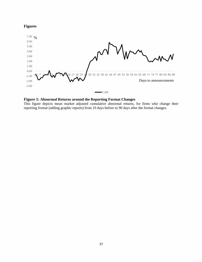
respectively. There is no significance for other windows as well. Figure 1 illustrates this

documented pattern in stock returns around the earnings announcements using daily returns. At

least, this shows that there was no additional positive information carried with the usually “cost

saving” excuses to stop delivering the graphically designed financial reports. Actually, for almost

all of the companies in our sample, the cost of adding the graphic fancy looking annual reports

can always be ignored in the earnings numbers.


[Insert Figure 1 about here]

4.3. Robustness

4.3.1. Matched Sample

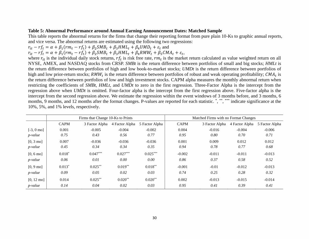
To verify the documented return pattern subsequent to the reporting format change, we

conduct various robustness tests. To deal with any selection bias, we re-do the same tests in Table

4 but use a different benchmark. Instead of comparing firms changing their reporting format

from plain 10-Ks to graphic annual reports and firms reverting back to plain 10-Ks, we study the

same first group of firms and their industry peers with similar size and financial report

readability. We report the results in Table 5, in which we don’t observe any significance for the

matched peers. This confirms the results found in Table 4.


13

4.3.2. Investor Sophistication

One might be curious if this anomaly has been studied yet? With the development of

information technologies, the computers are more and more powerful. Recently text mining

trading strategies has been become possible with the recent findings of informational contents

buried in the text and voice, such as financial report, IPO prospectus, and earnings calls (e.g.

Loughran & McDonald (2011, 2013, 2015), Engelberg & Parsons (2011), Jegadeesh & Wu

(2013)). As far as we know, there has no previous academic literature systematically studied the

information content embedded in the graphically designed financial reports. How about industry?

Literature in general agrees that institutional investors have more resources and are more

sophisticated. Have they already figured out the information in the prints? To answer the

question, we split our sample based on the institutional holdings. Table 6 reports the abnormal

returns around annual earnings announcement dates grouped by institutional ownership. The first

four columns report the abnormal returns for firms that change standard 10-Ks to beautifully-

designed annual reports for the firms with high institutional ownership, and the next four

columns report the abnormal returns for the firms with low institutional ownership for the same

time periods. Most of the numbers are positive and close to each other between the two groups.

E.g. the 6 months abnormal returns for the high institutional ownership group are 0.020 (p-value

=0.06), 0.023 (p-value = 0.06), 0.034 (p-value = 0.06), and 0.029 (p-value= 0.00) respectively

for CAPM, FF-3 factors model, 4-factor model, and FF-5 factors model, and the 6 months

abnormal returns for the low institutional ownership group are 0.020 (p-value = 0.08), 0.037 (p-

value = 0.06), 0.064 (p-value = 0.02), and 0.051 (p-value =0.00) for the CAPM, FF-3 factors

model, 4 factor model, and FF-5 factors model respectively. And the numbers are not statistically

different between the groups, which indicates that investor sophistication is not a plausible

14

channel for the positive relationship between reporting format change and subsequent stock

returns.


4.3.3. Information Asymmetry

Our results in the previous subsection indicate that the positive future stock performance

doesn’t disappear after controlling institutional ownership. Can information asymmetry explain

this interesting return pattern? Extant literature has suggested that companies’ stocks with higher

analyst coverage can be more efficient. The documented relationship between annual report

“graphicity” and subsequent stock returns may disappear if information asymmetry is the driver

of this relationship. To do so we split our sample based on the analyst coverage. Table 7 reports

the abnormal returns around annual earnings announcement dates grouped by analyst coverage.

The first four columns report the abnormal returns for firms that change standard 10-Ks to

beautifully-designed annual reports for the firms with high analyst coverage, and the next four

columns report the abnormal returns for the firms with low analyst coverage for the same time

periods. Again, most of the numbers are positive and close to each other between the two groups.

E.g. the 6 months abnormal returns for the high analyst coverage group are 0.019 (p-value =0.06),

0.021 (p-value = 0.04), 0.024 (p-value = 0.05), and 0.025 (p-value= 0.00) respectively for CAPM,

FF-3 factors model, 4-factor model, and FF-5 factors model, and the 6 months abnormal returns

for the low analyst coverage group are 0.021 (p-value = 0.08), 0.038 (p-value = 0.04), 0.068 (p-

value = 0.02), and 0.055 (p-value =0.01) for the CAPM, FF-3 factors model, 4 factor model, and

FF-5 factors model respectively. And these numbers are not statistically different between the

groups, which indicates that the information asymmetry is not a sound explanation for the

15

positive subsequent returns.


4.3.4. Stock Market Constraints

Stock market constraints such as short selling constraints affects market efficiency (see

e.g. Diamond & Verrecchia (1987), Bris et al. (2007), Boehmer and Wu (2013), and etc.). If short

selling constraints is a plausible channel to explain the documented relationship in this study, the

positive relationship between annual report format change and subsequent stock returns is

expected to be more pronounced for more constrained firms and to be negligible for heavily-

shorted firms. To test this conjecture, we split our sample based on the annual average short

interests the fiscal year before the earnings announcement. Table 8 reports the abnormal returns

around annual earnings announcement dates grouped by short interests. The first four columns

report the abnormal returns for firms that change standard 10-Ks to beautifully-designed annual

reports for the firms with high short interests, and the next four columns report the abnormal

returns for the firms with low short interests for the same time periods. Again, most of the

numbers are positive and close to each other between the two groups. E.g. the 6 months

abnormal returns for the high short interests group are 0.028 (p-value =0.07), 0.038 (p-value =

0.06), 0.033 (p-value = 0.05), and 0.035 (p-value= 0.00) respectively for CAPM, FF-3 factors

model, 4-factor model, and FF-5 factors model, and the 6 months abnormal returns for the low

analyst coverage group are 0.020 (p-value = 0.08), 0.057 (p-value = 0.04), 0.034 (p-value = 0.02),

and 0.031 (p-value =0.00) for the CAPM, FF-3 factors model, 4 factor model, and FF-5 factors

model respectively. And these numbers are not statistically different between the groups, which

indicates that the short selling constraints cannot explain the positive subsequent returns.


16

Given the results above, many alternative explanations don’t seem interpret the positive

subsequent returns. It suggests that the information content embedded in the graphic financial

reports have not been revealed by the market yet.

4.4. Hardening Existing Information or Delivering Additional Soft Information?

Liberti and Petersen (2018) characterize hard information and soft information. Hard

information is easy to measure and stone, and generally quantitative such as financial statements.

Usually, firms use numbers contained in financial statements to signal the financial market. As

the design of annual report that we study is part of the financial statements, a natural question to

ask would be “Are companies who add graphic elements to their annual reports trying to ‘harden’

the numeric information in the reports or just deliver additional soft information?”.

To answer this question, we study the short term stock prices variations around the

earnings announcements for the firms who added the graphic information to their annual

financial statements. We compute the market adjusted abnormal returns for the firms who add the

graphic information, and conduct an event study around the release date of the new graphic

financial report (e.g., the earnings announcement date). Table 9 reports the results. The

cumulative abnormal returns (CARs) for event windows of [-1,1], [0,1], and [-1,0] are all

statistically insignificant, suggesting that investors don’t react to this reporting format change.

The insignificant CARs of post event windows indicate that there are no post earnings

announcement drifts, consistent with our conjecture that the market fail to identify this additional

information until several months after the earnings announcement day.

In general, the results don’t support the “signaling” explanation, and suggest that the

newly added graphic reports are actually new additional information to the standard 10-Ks.

17

[Inset Table 9 about here]

4.5. Is This Soft Information Creditable?

So far, we have identified a possible information channel through which the insiders try

to deliver information to the market. Is this information creditable? Do firms really invest on

greater investment opportunities? We study the matched sample and employ the DiD method to

test the real activities afterwards. Table 10 reports multivariate DiD results on firm performance

and corporate investments around reporting format changes. The coefficients of Treatment

explain the main effect of the reporting format change. Column (1) reports the results of ROA as

the dependent variable with control variables and without controlling industry and year fixed

effects. Column (2) reports the results of CAPX as the dependent variable with control variables.

Column (3) reports the results of PPE as the dependent variable with control. We can find that

even though the ROA seems not be different between the treatment and control group. However,

the CAPX and PPE increased significant, with CAPX increases 2.406% (tstat = 1.67) on average,

and PPE increases by 13.09% (tstat=1.68) on average. And the increase is survived with the

industry fixed effects and year fixed effects as shown in columns (5) and (6).


We further employ placebo tests to check the robustness, and the results are reported in

Table 11. When we randomly change the year of adding graphic financial reports, we lost the

significance in CAPX and PPE as reported in Table 11, which further confirms the results

reported in Table 10.


18

5. Conclusion

Extant literature on financial reports content analysis focuses on the standard numbers or

textual information. With the help of computer programming, researchers have identified firm

valuation and performance relevant information by mining text readability, Fog index, and

sentiment. However, maybe because of lack of capability of analyzing non-textual information in

financial reports, prior literature neglects the existence of the financial reports’ overall design

and graphics information. On the one hand, all reported numbers and other statements in

financial reports are digitalized in the information era. On the other hand, it is hard to understand

why there are a high fraction of firms still providing print version graphic financial reports.

Managers might have tried to use the additional contents to deliver extra information. However,

due to computers are still lack of the capability to process the non-textual information, it is very

likely that it takes more time for such embedded information in the reports to be integrated into

the stock prices.

By examining the firms adding graphic print version financial reports in a large hand-

collected dataset, we find that those firms with newly added graphic financial reports earn at

least a positive 2.7% abnormal returns. And this finding is robust with different specifications.

Investor sophistication, financial market constraints, and information asymmetry don’t seem to

be the plausible explanations for this return pattern.

To further disentangle whether firms use the graphic information as additional message or

just strengthening the existing numbers in 10-Ks, we conduct a short term event study. Our

results suggest that the newly added graphic reports convey new additional information rather

than “hardening” the existing information.

In order to pursue the reasons or the tendency why firms choose to add graphic financial

19

report, we match the firms with newly added print financial reports by size, industry, and

readability, and form a control group. Then, we conduct DiD tests. With the powerful DiD tests,

we further find that firms increased CAPX and PPE in the next fiscal year or two after they add

print version financial reports, which implies that these group of firms have real growth that

brings in superior performance.

Overall, our study suggests that not only texts but also graphics embedded in the financial

report contains material information to the public. The underlying drivers and explanations

behind this newly found anomaly is worth to pursue in the future studies.

20

Reference

Barber, B. M., & Odean, T. (2008). All that glitters: The effect of attention and news on the

buying behavior of individual and institutional investors. Review of Financial

Studies, 21(2), 785-818.

Benefield, J. D., Cain, C. L., & Johnson, K. H. (2011). On the relationship between property

price, time-on-market, and photo depictions in a multiple listing service. The Journal of

Real Estate Finance and Economics, 43(3), 401-422.

Boehmer, E., & Wu, J. J., (2013). Short selling and the price discovery process. Review of

Financial Studies, 26(2), 287-322.

Bris, A., Goetzmann, N. W., & Zhu, N., (2007). Efficiency and the bear: short sales and markets

around the world. The Journal of Finance, 62(3), 1029-1079.

Carrillo, P. E. (2008). Information and real estate transactions: the effects of pictures and virtual

tours on home sales. George Washington University Working Paper.

Diamond, D. W., & Verrechia, R. E., (1987). Constraints on short-selling and asset price

adjustment to private information. Journal of Financial Economics, 18(2), 277-311.

DellaVigna, S., & Pollet, J. M. (2009). Investor inattention and Friday earnings

announcements. The Journal of Finance, 64(2), 709-749.

Engelberg, J. E., & Parsons, C. A. (2011). The causal impact of media in financial markets. The

Journal of Finance, 66(1), 67-97.

Feng, D. (2011). Visual Space and Ideology: A Critical Cognitive Analysis of Spatial

Orientations in Advertising. In Kay L. O'Halloran and Bradley A. Smith, B. A. (eds),

Multimodal Studies: Exploring Issues and Domains. New York & London: Routledge.

Goeij, P. D., Hogendoorn, T., & Campenhout, G. V. (2014). Pictures are worth a thousand words:

Graphical information and investment decision making. Working paper.

Halliday, M. (1994). An Introduction to Functional Grammar (2nd edition). London: Arnold.

Hanley, K. W., & Hoberg, G. (2010). The information content of IPO prospectuses. Review of

Financial Studies, 23(7), 2821-2864.

Hirshleifer, D., Lim, S. S., & Teoh, S. H. (2009). Driven to distraction: Extraneous events and

underreaction to earnings news. The Journal of Finance, 64(5), 2289-2325.

Hoberg, G., & Phillips, G. (2010). Product market synergies and competition in mergers and

acquisitions: A text-based analysis. Review of Financial Studies, 23(10), 3773-3811.

Jegadeesh, N., & Wu, D. (2013). Word power: A new approach for content analysis. Journal of

21

Financial Economics, 110(3), 712-729.

Li, F. (2008). Annual report readability, current earnings, and earnings persistence. Journal of

Accounting and economics, 45(2), 221-247.

Li, F. (2010). The Information Content of Forward‐Looking Statements in Corporate Filings—

A Naïve Bayesian Machine Learning Approach. Journal of Accounting Research, 48(5),

1049-1102.

Liberti, M., & Petersen, M. (2018). Information: Hard and Soft. Working paper.

Loughran, T., & McDonald, B. (2011). When is a liability not a liability? Textual analysis,

dictionaries, and 10‐Ks. The Journal of Finance, 66(1), 35-65.

Loughran, T., & McDonald, B. (2013). IPO first-day returns, offer price revisions, volatility, and

form S-1 language. Journal of Financial Economics, 109(2), 307-326.

Loughran, T., & McDonald, B. (2015). The use of word lists in textual analysis. Journal of

Behavioral Finance, 16(1), 1-11.

Tetlock, Paul C., (2007). Giving content to investor sentiment: The role of media in the stock

market, Journal of Finance, 62, 1139–1168.

Twedt, B., & Rees, L. (2012). Reading between the lines: an empirical examination of qualitative

attributes of financial analysts’ reports. Journal of Accounting and Public Policy, 31(1), 1-

21.

Ventola, E., & Guijarro, A.J.M. (2009). The World Told and the World Shown: Multisemiotic

Issues. Hampshire: Palgrave Macmillan.

Wignell, P. (2011). Picture Books for Young Children of Different Ages: The Changing

Relationships between Images and Words. In Kay L. O'Halloran and Bradley A. Smith, B.

A. (eds), Multimodal Studies: Exploring Issues and Domains. New York & London:

Routledge.

Wohlwend, K. (2011). Mapping Modes in Children’s Play and Design: An Action-oriented

Approach to Critical Multimodal Analysis. In R. Rogers (Ed.), An Introduction to Critical

Discourse Analysis in Education (pp. 23-45). New York, NY: Routledge.

22

Appendix

Appendix 1: Variable Definitions

Variables Definition

After Dummy variable equal to 1 if the fiscal year is after the reporting format

changes from pure plain 10-Ks to graphic annual reports and equal to 0 if the

fiscal year is before the changes

Asset Growth Total Assets (AT) divided by start-of-year Total Assets minus one x 100

Accruals Accruals: it is calculated as discretionary accruals (Dechow et al. 1995)

Analyst Coverage Number of analysts following the company immediately before the earnings

announcement date

CAPX Capital expenditures (Compustat CAPX) scaled by end-of-year total assets

(AT) x 100

CAPX&RD Capital expenditures (CAPX) plus Research and Development Expenses

(XRD) scaled by end-of-year total assets (AT) x 100

CEO Letter Dummy variable equal to 1 if the there is a CEO letter in the graphic annual

report in the fiscal year, and 0 if else.

CEO Picture Dummy variable equal to 1 if the there is a picture of the CEO in the graphic

annual report in the fiscal year, and 0 if else.

CEO Signature Dummy variable equal to 1 if the there is a CEO signature in the graphic

annual report in the fiscal year, and 0 if else.

Change to 10-Ks Dummy variable equal to 1 if the firm changes their reporting format from a

graphic annual report to a pure plain 10-K, and 0 if else.

Change to Prints Dummy variable equal to 1 if the firm changes their reporting format from

pure plain 10-K to a graphic annual report, and 0 if else.

Institutional Ownership Institutional ownership in percentage immediately before the earnings

announcement date

Leverage Long term debt (DLTT) plus debt in current liabilities (DLC) scaled by the

sum of long term debt, debt in current liabilities, and total stockholders' equity

(SEQ) x 100

Number of Graphic

Pages

The number of pages with colorful pages in the graphic annual reports

PPE Property, plant, and equipment net

Prints Dummy variable equal to 1 if the firms use graphic annual reports in the fiscal

year, and 0 if else.

Q Tobin's Q is defined as market value of equity (PRCC x CSHO) plus book

value of assets minus book value of equity minus deferred taxes (when

available) (AT-CEQ-TXDB), scaled by book value of total assets (AT).

Variable is lagged one year

Readability Fog Readability index

ROA Return on assets

ROE Return on equity

Sales Growth Sales dividend by the start-of-year sales minus one x 100

Short Interests Yearly average of short interests / volume immediately before the earnings

announcement date

23

Appendix 1, cont’d Total Assets Firm level total assets (in Millions USD)

Treatment Dummy variable equal to 1 if the company experiences any format change from

pure plain 10-Ks to graphic annual reports and its fiscal year during the period

between 1 year and 2 years after this change. The dummy variable is equal to 0

when the firm years in the control group 2 years before and after their paired firms'

format changes, and for the firms that add print financial reports pure plain 10-Ks

before the format changes.

24

Appendix 2: An Example: AIRM

Air Methods (Ticker: AIRM) changes their reporting format from a pure plain 10-K to a graphic

annual report style in the fiscal year of 2011. From the following, we show the cover pages of

their annual reports in 2010 and 2011 FY as well as the daily stock prices around this format

change. We can observe the significant changes in their reporting format, and how their share

prices perform after the format change.

The Cover Page of AIRM’s Annual Report for 2010 Fiscal Year

The Cover Page of AIRM’s Annual Report for 2011 Fiscal Year

25

Snapshot from Yahoo Finance: Daily Stock Prices from Feb, 2012-Oct, 2012 with the Annual

Earnings Announcement Date of April 10, 2012

26

Tables

Table 1: The Characteristics of Annual Reports/10-Ks

This table reports the descriptive statistics of the characteristics of all manually collected annual

reports/10-Ks for all sample firms from S&P 1500. All variables are defined in Appendix 1.

Variable No. of Firms Mean Median Std. Dev. Max. Min.

Prints 758 0.722 1.000 0.449 2.000 0.000

Number of

Graphic Pages 758 6.470 4.000 9.293 83.00 0.000

CEO Letter 758 0.761 1.000 0.427 2.000 0.000

CEO Signature 758 0.739 1.000 0.442 2.000 0.000

CEO Picture 758 0.509 1.000 0.500 1.000 0.000

Change to 10-Ks 758 0.035 0.000 0.183 1.000 0.000

Change to Prints 758 0.026 0.000 0.159 1.000 0.000

27

Table 2: Firm Characteristics before Reporting Format Changes

This table reports summary statistics of firm characteristics for both two groups in the matched

sample one fiscal year immediately before the format changes from pure plain 10-Ks to graphic

annual reports. The first group includes all firms that experience such format changes. The second

group is formed by matching by total assets, industry, and readability with the firms in the

treatment group. The t-stats for mean test and chi-sq for median test are also reported. All variables

are winsorized at 1% and 99% level. ***, **, and * indicate significance at the 1%, 5%, and 10%

levels. All variables have defined in appendix.

Firms Changing to Prints

Matched Firms with no

Format Changes Test for Differences

Variable N Mean Median SD N Mean Median SD Mean

(t-stats)

Median

(chi-sq)

Total Assets 64 3,050 630.2 8,571 61 5,318 729.9 25,374 -0.67 0.96

ROA 54 12.63 12.44 9.89 54 11.35 10.56 10.78 0.64 0.44

ROE 54 23.03 22.08 22.13 54 21.62 20.08 26.10 0.30 0.44

Sales Growth 54 10.89 14.49 21.25 52 11.25 10.60 25.14 -0.08 0.69

Asset Growth 54 7.716 5.556 19.10 54 11.60 6.089 28.24 -0.83 0.00

CAPX 55 4.124 2.801 3.911 56 4.320 2.628 4.508 -0.24 0.44

CAPX&RD 34 8.639 7.698 6.907 37 9.091 6.48 8.204 -0.25 1.13

Leverage 54 18.87 5.47 22.33 54 20.20 17.13 22.57 -0.30 0.59

Readability 36 18.16 17.91 3.238 22 18.02 18.12 2.692 0.17 0.29

28

Table 3: Firm Characteristics and the Addition of Prints

This table reports the logistic regression results that identify the characteristics of the firms who

added print financial reports. Columns (1) through (5) report the results of CAPX, Q, Size, and

Readability-index as the independent variable without controlling other firm characteristics.

Column (6) reports the results of all above variables as the independent variables with control

variables. T-statistics are displayed in the parenthesis under each coefficient. Standard errors

adjust for heteroskedasticity and clustered by firm. *, **, *** indicate significance at the 1%, 5%,

and 10% levels respectively. All variables are defined in Appendix 1.

(1) (2) (3) (4) (5) (6)

Prints Prints Prints Prints Prints Prints

CAPX -0.014

-0.033

(-0.50)

(-0.78)

Accurals

-0.310**

-0.469*

(-2.25)

(-1.69)

Q

-0.079

-0.113

(-0.74)

(-0.52)

Size

0.381***

0.335*

(3.34)

(1.80)

Readability-Index

0.048* 0.107**

(1.71) (2.19)

Leverage

-0.004

(-0.34)

Past Profitability

0.024

(1.15)

N 602 519 600 613 279 196

pseudo R-sq 0.001 0.010 0.001 0.035 0.003 0.056

29

Table 4: Abnormal Performance around Annual Earning Announcement Dates

This table reports the abnormal returns for the firms that change their reporting format from pure plain 10-Ks to graphic annual reports,

and vice versa. The abnormal returns are estimated using the following two regressions:

𝑟𝑖𝑡 − 𝑟𝑓𝑡 = 𝛼 + 𝛽1(𝑟𝑚𝑡 − 𝑟𝑓𝑡) + 𝛽2𝑆𝑀𝐵𝑡 + 𝛽3𝐻𝑀𝐿𝑡 + 𝛽4𝑈𝑀𝐷𝑡 + 𝜀𝑡 and

𝑟𝑖𝑡 − 𝑟𝑓𝑡 = 𝛼 + 𝛽1(𝑟𝑚𝑡 − 𝑟𝑓𝑡) + 𝛽2𝑆𝑀𝐵𝑡 + 𝛽3𝐻𝑀𝐿𝑡 + 𝛽4𝑅𝑀𝑊𝑡 + 𝛽5𝐶𝑀𝐴𝑡 + 𝜀𝑡, where 𝑟𝑖𝑡 is the individual daily stock returns, 𝑟𝑓𝑡 is risk free rate, 𝑟𝑚𝑡 is the market return calculated as value weighted return on all

NYSE, AMEX, and NASDAQ stocks from CRSP. SMBt is the return difference between portfolios of small and big stocks; HMLt is

the return difference between portfolios of high and low book-to-market stocks; UMDt is the return difference between portfolios of

high and low prior-return stocks; 𝑅𝑀𝑊𝑡 is the return difference between portfolios of robust and weak operating profitability; 𝐶𝑀𝐴𝑡 is

the return difference between portfolios of low and high investment stocks. CAPM alpha measures the monthly abnormal return when

restricting the coefficients of SMBt, HMLt, and UMDt to zero in the first regression. Three-Factor Alpha is the intercept from the

regression above when UMDt is omitted. Four-factor alpha is the intercept from the first regression above. Five-factor alpha is the

intercept from the second regression above. We estimate the regression within the event windows of 3 months before, and 3 months, 6

months, 9 months, and 12 months after the format changes. P-values are reported for each statistic. *, **, *** indicate significance at the

10%, 5%, and 1% levels, respectively.

Firms that Change 10-Ks to Prints Firms that Change Prints to 10-Ks

CAPM 3 Factor Alpha 4 Factor Alpha 5 Factor Alpha CAPM 3 Factor Alpha 4 Factor Alpha 5 Factor Alpha

[-3, 0 mo] 0.001 -0.005 -0.004 -0.002 0.003 -0.015 -0.004 -0.003

p-value 0.75 0.43 0.56 0.77 0.97 0.80 0.72 0.65

[0, 3 mo] 0.007 -0.036 -0.036 -0.036 0.001 0.009 0.010 0.010

p-value 0.45 0.34 0.34 0.35 0.95 0.78 0.74 0.75

[0, 6 mo] 0.018* 0.047*** 0.027*** 0.025*** -0.001 -0.010 -0.010 -0.011

p-value 0.06 0.01 0.00 0.00 0.88 0.31 0.52 0.54

[0, 9 mo] 0.013* 0.025** 0.019** 0.018** -0.001 -0.011 -0.011 -0.011

p-value 0.09 0.05 0.02 0.03 0.84 0.24 0.28 0.32

[0, 12 mo] 0.014 0.025** 0.020** 0.020** 0.000 -0.012 -0.010 -0.010

p-value 0.14 0.04 0.02 0.03 0.97 0.21 0.32 0.37

30

Table 5: Abnormal Performance around Annual Earning Announcement Dates: Matched Sample

This table reports the abnormal returns for the firms that change their reporting format from pure plain 10-Ks to graphic annual reports,

and vice versa. The abnormal returns are estimated using the following two regressions:












Firms that Change 10-Ks to Prints Matched Firms with no Format Changes


[-3, 0 mo] 0.001 -0.005 -0.004 -0.002 0.004 -0.016 -0.004 -0.006

p-value 0.75 0.43 0.56 0.77 0.95 0.80 0.70 0.71

[0, 3 mo] 0.007 -0.036 -0.036 -0.036 0.001 0.009 0.012 0.012

p-value 0.45 0.34 0.34 0.35 0.94 0.78 0.77 0.68

[0, 6 mo] 0.018* 0.047*** 0.027*** 0.025*** -0.002 -0.011 -0.011 -0.013

p-value 0.06 0.01 0.00 0.00 0.86 0.37 0.58 0.52

[0, 9 mo] 0.013* 0.025** 0.019** 0.018** -0.001 -0.01 -0.012 -0.013

p-value 0.09 0.05 0.02 0.03 0.74 0.25 0.28 0.32

[0, 12 mo] 0.014 0.025** 0.020** 0.020** 0.002 -0.013 -0.015 -0.014

p-value 0.14 0.04 0.02 0.03 0.95 0.41 0.39 0.41

31

Table 6: Abnormal Performance around Annual Earning Announcement Dates, Grouped by Institutional Ownership

This table reports the mean abnormal returns for the firms that change their reporting format from pure plain 10-Ks to graphic annual

reports grouped by institutional ownership before the format changes. The abnormal returns are estimated using the following two

regressions:












Firms with Higher Institutional Ownership Firms with Lower Institutional Ownership


[-3, 0 mo] 0.002 0.004 0.001 0.002 0.004 -0.016 -0.004 -0.006

p-value 0.70 0.41 0.32 0.83 0.95 0.80 0.70 0.71

[0, 3 mo] 0.028* -0.023 -0.023 -0.021 0.031 -0.023 -0.023 0.011

p-value 0.06 0.67 0.67 0.35 0.21 0.61 0.61 0.70

[0, 6 mo] 0.020* 0.023* 0.034* 0.029*** 0.020* 0.037* 0.064** 0.051***

p-value 0.06 0.06 0.06 0.00 0.08 0.06 0.02 0.00

[0, 9 mo] 0.015 0.016* 0.018* 0.017** 0.015 0.027* 0.035* 0.030**

p-value 0.13 0.10 0.10 0.03 0.41 0.09 0.08 0.04

[0, 12 mo] 0.017* 0.017* 0.018 0.020** 0.016 0.026* 0.035* 0.030**

p-value 0.09 0.09 0.13 0.03 0.37 0.09 0.07 0.03

32

Table 7: Abnormal Performance around Annual Earning Announcement Dates, Grouped by Analyst Coverage


reports grouped by analyst coverage before the format changes. The abnormal returns are estimated using the following two

regressions:












Firms with Higher Analyst Coverage Firms with Lower Analyst Coverage


[-3, 0 mo] 0.001 -0.007 -0.006 -0.004 0.003 -0.012 -0.001 -0.002

p-value 0.52 0.35 0.49 0.81 0.95 0.80 0.70 0.71

[0, 3 mo] 0.023* -0.022 -0.013 -0.022 0.032 -0.019 -0.013 0.003

p-value 0.06 0.67 0.67 0.35 0.21 0.58 0.45 0.87

[0, 6 mo] 0.019* 0.021** 0.024** 0.025*** 0.021* 0.038** 0.068** 0.055***

p-value 0.06 0.04 0.05 0.00 0.08 0.04 0.02 0.01

[0, 9 mo] 0.015* 0.013* 0.017* 0.015** 0.019 0.029* 0.032* 0.041**

p-value 0.09 0.10 0.10 0.03 0.41 0.08 0.09 0.02

[0, 12 mo] 0.017* 0.018 0.016 0.019 0.019* 0.036* 0.035* 0.031**

p-value 0.09 0.19 0.13 0.20 0.10 0.09 0.06 0.04

33

Table 8: Abnormal Performance around Annual Earning Announcement Dates, Grouped by Short Interests


reports grouped by short interests before the format changes. The abnormal returns are estimated using the following two regressions:












Firms with Higher Short Interests Firms with Lower Short Interests


[-3, 0 mo] 0.001 -0.001 -0.002 -0.001 0.004 -0.005 -0.003 -0.004

p-value 0.45 0.25 0.36 0.75 0.55 0.48 0.35 0.57

[0, 3 mo] 0.028* -0.023 -0.023 -0.021 0.031 -0.023 -0.023 0.011

p-value 0.07 0.72 0.57 0.35 0.21 0.61 0.61 0.70

[0, 6 mo] 0.028* 0.038* 0.033** 0.035*** 0.020* 0.057** 0.034** 0.031***

p-value 0.07 0.06 0.05 0.00 0.08 0.04 0.02 0.00

[0, 9 mo] 0.015 0.016* 0.018* 0.017** 0.017* 0.019** 0.025** 0.029**

p-value 0.13 0.09 0.08 0.03 0.09 0.05 0.03 0.04

[0, 12 mo] 0.016 0.019 0.018 0.016 0.017 0.020* 0.024** 0.025**

p-value 0.09 0.22 0.19 0.30 0.11 0.09 0.05 0.03

34

Table 9: Multivariate DiD Results: Firm Performance and Corporate Investments around

Reporting Format Changes

This table reports the mean abnormal returns for the firms that change their reporting format

from pure plain 10-Ks to graphic annual reports grouped. We compute the abnormal returns

using market model, within the event windows of 1 day before to 1 day after, 1 day after to 10

days after, and to 30 days after the format changes. P-values are reported for each statistic. *, **, *** indicate significance at the 10%, 5%, and 1% levels, respectively.

[-1, 0] [0, 1] [-1, 1] [1, 10] [1, 30]

CAR 0.002 0.003 0.009 0.008 -0.008

P-value 0.45 0.34 0.48 0.49 0.48

35

Table 10: Multivariate DiD Results: Firm Performance and Corporate Investments around

Reporting Format Changes

This table reports the regression results that estimate differences in treated and their paired firms’

firm performance and corporate investment around the reporting format changes. Column (1)

reports the results of ROA as the dependent variable with control variables and without

controlling industry and year fixed effects. Column (2) reports the results of CAPX as the

dependent variable with control variables and without controlling industry and year fixed effects.

Column (3) reports the results of PPE as the dependent variable with control variables and

without controlling industry and year fixed effects. Column (4) reports the results of ROA as the

dependent variable with control variables and controlling industry and year fixed effects. Column

(5) reports the results of CAPX as the dependent variable with control variables and controlling

industry and year fixed effects. Column (6) reports the results of PPE as the dependent variable

with control variables and controlling industry and year fixed effects. T-statistics are displayed in

the parenthesis under each coefficient. Standard errors adjust for heteroskedasticity and clustered

by firm. *, **, *** indicate significance at the 1%, 5%, and 10% levels respectively. All variables

are defined in Appendix 1.

(1) (2) (3) (4) (5) (6)

ROA CAPX PPE ROA CAPX PPE

After 2.076 -0.911 -7.617 3.013 0.223 -0.419

(1.54) (-0.73) (-1.19) (1.01) (0.12) (-0.05)

Treatment -1.129 2.406* 13.09* -0.789 1.941* 5.529*

(-0.87) (1.67) (1.68) (-0.30) (1.69) (1.67)

Size 0.279 -0.227 -0.823 0.861 -0.333 -4.839**

(0.49) (-0.63) (-0.25) (0.71) (-0.73) (-2.17)

Leverage 0.020 0.038* 0.592*** 0.008 0.014 0.331**

(0.63) (1.95) (3.44) (0.12) (0.43) (2.11)

Readability-Index -0.524* -0.025 0.687 -0.682** -0.043 0.655

(-1.76) (-0.24) (0.70) (-2.36) (-0.55) (1.09)

Past Profitability 0.756*** 0.161*** 0.782*** 0.552*** 0.113*** 0.242

(6.82) (5.06) (3.76) (3.75) (3.19) (1.27)

Industry Fixed Effects No No No Yes Yes Yes

Year Fixed Effects No No No Yes Yes Yes

N 160 160 157 160 160 157

adj. R-sq 0.548 0.134 0.193 0.627 0.455 0.695

36

Table 11: Placebo Tests

This table reports Placebo tests results when we define the event year as “Pseudo Event” year.

Panel A reports the placebo tests results when we use the third year before the format change as

the “Pseudo Event” year for all firms. Panel B reports the placebo tests results when we use the

third year after the format change as the “Pseudo Event” year for all firms. Columns 1 and 2

report the results of dependent variables as CAPX and PPE without controlling year and industry

fixed effects; Columns 3 and 4 report the results of dependent variables as CAPX and PPE with

controlling year and industry fixed effects. T-statistics are displayed within parentheses under

each coefficient. Standard errors adjust for heteroskedasticity and within correlation clustered by

firm. All variables are defined in Appendix 1. *, **, *** indicate significance at the 1%, 5%, and 10%

levels respectively.

CAPX PPE CAPX PPE

Panel A: Year of Format Changes=-3

Treatment -1.604 10.69 0.490 0.001

(-0.46) (0.83) (0.19) (0.00)

with Controls Yes Yes Yes Yes

Year/Industry Fixed Effects No No Yes Yes

Panel B: Year of Format Changes=+3

Treatment 0.929 -2.482 1.540 -3.746

(0.63) (-0.22) (1.28) (-0.50)

with Controls Yes Yes Yes Yes

Year/Industry Fixed Effects No No Yes Yes

37

Figures

Figure 1: Abnormal Returns around the Reporting Format Changes This figure depicts mean market adjusted cumulative abnormal returns, for firms who change their

reporting format (adding graphic reports) from 10 days before to 90 days after the format changes.

-3.00

-2.00

-1.00

0.00

1.00

2.00

3.00

4.00

5.00

6.00

7.00

-10 -7 -4 -1 2 5 8 11 14 17 20 23 26 29 32 35 38 41 44 47 50 53 56 59 62 65 68 71 74 77 80 83 86 89

CAR

Days to announcements

%

Date post:	09-Jan-2022
Category:	Documents
Upload:	others
View:	1 times
Download:	0 times

Annual Report Graphicity and Stock Returns

Documents