Journal of Monetary Economics 50 (2003) 745–787 . A no-arbitrage vector autoregression of term structure dynamics with macroeconomic and latent variables $ Andrew Ang a,b, *, Monika Piazzesi b,c a Columbia Business School, 3022 Broadway, 805 Uris, New York, NY 10027, USA b National Bureau of Economic Research, Cambridge, MA 02138, USA c Anderson Graduate School of Management, UCLA, 110 Westwood Plaza, Box 951481, Los Angeles, CA 90095-1481, USA Received 14 June 2000; received in revised form 29 January 2002; accepted 24 July 2002 Abstract We describe the joint dynamics of bond yields and macroeconomic variables in a Vector Autoregression, where identifying restrictions are based on the absence of arbitrage. Using a term structure model with inflation and economic growth factors, together with latent variables, we investigate how macro variables affect bond prices and the dynamics of the yield curve. We find that the forecasting performance of a VAR improves when no-arbitrage restrictions are imposed and that models with macro factors forecast better than models with only unobservable factors. Variance decompositions show that macro factors explain up to 85% of the variation in bond yields. Macro factors primarily explain movements at the short ARTICLE IN PRESS $ We have had helpful discussions with Geert Bekaert, Mike Chernov, John Cochrane, Darrell Duffie, Charles Evans, Mark Ferguson, Joel Hasbrouck, Bob Hodrick, Avi Kamara, Jun Liu, David Marshall, Jun Pan, Thomas Sargent, Stephen Schaefer, Martin Schneider, Ken Singleton, Suresh Sundaresan, Chris Telmer and Jessica Wachter. We thank seminar participants at Columbia University, NYU, the NBER Summer Institute, the American Economics Association, the Western Finance Association, and the Seventh World Congress of the Econometric Society. We thank Marty Eichenbaum (the editor) and we are grateful for extremely helpful comments from an anonymous referee. Andrew Ang acknowledges funding from the National Science Foundation. *Corresponding author. Professor Andrew Ang, Business School, Columbia University, 3022 Broadway, 805 Uris, New York, NY 10027, USA. Tel.: +1-212-854-9154; fax: +1-212-662-8474. E-mail address: [email protected] (A. Ang). URL: http://www.columbia.edu/~aa610. 0304-3932/03/$ - see front matter r 2003 Elsevier Science B.V. All rights reserved. doi:10.1016/S0304-3932(03)00032-1
Transcript
Journal of Monetary Economics 50 (2003) 745–787
.
A no-arbitrage vector autoregression of termstructure dynamics with macroeconomic and
latent variables$
Andrew Anga,b,*, Monika Piazzesib,c
aColumbia Business School, 3022 Broadway, 805 Uris, New York, NY 10027, USAbNational Bureau of Economic Research, Cambridge, MA 02138, USA
cAnderson Graduate School of Management, UCLA, 110 Westwood Plaza, Box 951481,
Los Angeles, CA 90095-1481, USA
Received 14 June 2000; received in revised form 29 January 2002; accepted 24 July 2002
Abstract
We describe the joint dynamics of bond yields and macroeconomic variables in a Vector
Autoregression, where identifying restrictions are based on the absence of arbitrage. Using a
term structure model with inflation and economic growth factors, together with latent
variables, we investigate how macro variables affect bond prices and the dynamics of the yield
curve. We find that the forecasting performance of a VAR improves when no-arbitrage
restrictions are imposed and that models with macro factors forecast better than models with
only unobservable factors. Variance decompositions show that macro factors explain up to
85% of the variation in bond yields. Macro factors primarily explain movements at the short
ARTICLE IN PRESS
$We have had helpful discussions with Geert Bekaert, Mike Chernov, John Cochrane, Darrell Duffie,
Charles Evans, Mark Ferguson, Joel Hasbrouck, Bob Hodrick, Avi Kamara, Jun Liu, David Marshall,
Jun Pan, Thomas Sargent, Stephen Schaefer, Martin Schneider, Ken Singleton, Suresh Sundaresan, Chris
Telmer and Jessica Wachter. We thank seminar participants at Columbia University, NYU, the NBER
Summer Institute, the American Economics Association, the Western Finance Association, and the
Seventh World Congress of the Econometric Society. We thankMarty Eichenbaum (the editor) and we are
grateful for extremely helpful comments from an anonymous referee. Andrew Ang acknowledges funding
from the National Science Foundation.
*Corresponding author. Professor Andrew Ang, Business School, Columbia University, 3022
Broadway, 805 Uris, New York, NY 10027, USA. Tel.: +1-212-854-9154; fax: +1-212-662-8474.
0304-3932/03/$ - see front matter r 2003 Elsevier Science B.V. All rights reserved.
doi:10.1016/S0304-3932(03)00032-1
end and middle of the yield curve while unobservable factors still account for most of the
movement at the long end of the yield curve.
r 2003 Elsevier Science B.V. All rights reserved.
JEL classification: C13; C32; E43; E44; E52
Keywords: Estimation; Time series models; Determination of interest rates; Financial markets and the
macroeconomy; Monetary policy
1. Introduction
Describing the joint behavior of the yield curve and macroeconomic variables isimportant for bond pricing, investment decisions and public policy. Many termstructure models have used latent factor models to explain term structuremovements, and although there are some interpretations to what these factorsmean, the factors are not given direct comparisons with macroeconomic variables.For example, Pearson and Sun (1994)’s factors are labeled ‘‘short rate’’ and‘‘inflation’’, but their estimation does not use inflation data. The terms ‘‘short rate’’and ‘‘inflation’’ are just convenient names for the unobserved factors. Anotherexample is Litterman and Scheinkman (1991), who call their factors ‘‘level,’’ ‘‘slope’’and ‘‘curvature’’. Similarly, Dai and Singleton (2000) use the words ‘‘level,’’ ‘‘slope’’and ‘‘butterfly’’ to describe their factors. These labels stand for the effect the factorshave on the yield curve rather than describing the economic sources of the shocks.
In the absence of a workhorse general equilibrium model for asset pricing (seeHansen and Jagannathan, 1991), factor models have the advantage that they onlyimpose no-arbitrage conditions and not all other conditions that characterize theequilibrium in the economy. Most existing factor models of term structure areunsatisfactory, however, because they do not model how yields directly respond tomacroeconomic variables.1 In contrast, empirical studies try to directly model therelationships between bond yields and macro variables by using vector autore-gressive (VAR) models. Studies like Estrella and Mishkin (1997) and Evans andMarshall (1998) use VARs with yields of various maturities together with macrovariables. These studies infer the relationships between yield movements and shocksin macro variables using impulse responses (IRs) and variance decompositiontechniques implied from the VAR. For example, Evans and Marshall (2001)associate shocks to economic activity and price levels with level effects across theyield curve. Another type of shock, which can be identified with various schemes,comes from monetary policy.2
ARTICLE IN PRESS
1The exception is Piazzesi (2001), who develops a term structure model with interest-rate targeting by
the central bank. In the model, the central bank reacts to macroeconomic variables such as nonfarm
payroll employment.2See, for example, Gali (1992), Sims and Zha (1995), Bernanke and Mihov (1998), Christiano, et al.
(1996), and Uhlig (2001). For a survey, see Christiano, et al. (1999).
A. Ang, M. Piazzesi / Journal of Monetary Economics 50 (2003) 745–787746
Existing macro VAR studies are characterized by three features. First, onlymaturities whose yields which have been included in the VAR may have theirbehavior directly inferred by the dynamics of the VAR. As an unrestricted VAR isgenerally not a complete theory of the term structure, it says little about how yieldsof maturities not included in the VAR may move. Second, the implied movements ofyields in relation to each other may not rule out arbitrage opportunities when thecross-equation restrictions implied by this assumption are not imposed in theestimation. Finally, unobservable variables cannot be included as all variables inthe VAR must be observable. The VAR approach, however, is very flexible, and theimplied impulse response functions (IRs) and variance decompositions give insightsinto the relationships between macro-shocks and movements in the yield curve.
A related asset-pricing literature beginning with Sargent (1979) has tried toestimate VAR systems of yields under the null of the Expectations Hypothesis (seeBekaert and Hodrick, 2001). These systems do not contain macro variables, which isthe focus of our paper. Moreover, expected excess returns on US bonds vary overtime (see, for example, Campbell and Shiller, 1991). The term structure dynamics inthis paper are therefore given by a Gaussian term structure model with time-varyingrisk premia, consistent with deviations from the Expectations Hypothesis (see Fisher,1998; Duffee, 2002; Dai and Singleton, 2002).
We incorporate macro variables as factors in a term structure model by using afactor representation for the pricing kernel, which prices all bonds in the economy.This is a direct and tractable way of modelling how macro factors affect bond prices.The pricing kernel is driven by shocks to both observed macro factors andunobserved factors. Since macro factors are correlated with yields, incorporatingthese factors may lead to models whose forecasts are better than models which omitthese factors. We investigate whether the purely unobservable factors of multi-factorterm structure models can be explained by macro variables, and we examine how thelatent factors change when macro variables are incorporated into such models.
Our methodology gives us several advantages over existing empirical VARapproaches. First, it allows us to characterize the behavior of the entire yield curve inresponse to macro shocks rather than just the yields included in the VAR. Second, adirect comparison of macro variables with latent yield factors can be made. Third,variance decompositions and other methods can estimate the proportion of termstructure movements attributable to observable macro shocks, and other latentvariables. Finally, our approach retains the tractability of the VAR approachesbecause we estimate a VAR subject to nonlinear no-arbitrage restrictions.
Our term structure model is Gaussian, so it is a VAR model, and IRs and variancedecompositions can be easily computed. Formally, our model is a special case ofdiscrete-time versions of the affine class introduced by Duffie and Kan (1996), wherebond prices are exponential affine functions of underlying state variables. In ourmodel, however, some of the state variables are observed macroeconomic aggregates.With Gaussian processes, the affine model reduces to a VAR with cross-equationrestrictions. Our set-up accommodates lags in the driving factors and allows us tocompute variance decompositions where we can attribute the proportion ofmovements in the yield curve to observable and unobservable factors. We can plot
ARTICLE IN PRESSA. Ang, M. Piazzesi / Journal of Monetary Economics 50 (2003) 745–787 747
IRs of shocks to various factors on any yield, since the no-arbitrage model gives usbond prices for all maturities.
We obtain our measures of inflation and real activity by extracting principalcomponents of two groups of variables that are selected to represent measures ofprice changes and economic growth. These factors are then augmented by latentvariables. As term structure studies have suggested up to three latent factors asappropriate to capture most salient features of the yield curve, we estimate modelswith three latent factors in addition to the macro variables. Our main model hasthree correlated unobservable factors, together with the two macro factors (inflationand real economic activity).
Imposing no-arbitrage restrictions improves out-of-sample forecasts from a VAR.Forecasts can be further improved by incorporating macro factors into models withlatent variables. We show that a significant part of the latent factors implied bytraditional models with only latent yield variables can be attributed to macrovariables. In particular, ‘‘slope’’ and ‘‘curvature’’ factors can be related to macrofactors, while the ‘‘level’’ factor survives largely intact when macro variables areincorporated.
We find that macro factors explain a significant amount of the variation in bondyields. Macro factors explain up to 85% of the forecast variance for long forecasthorizons at short and medium maturities of the yield curve. The proportion of theforecast variance of yields attributable to macro factors decreases at longer yields. Atthe long end of the yield curve, 60% of the forecast variance is attributable to macrofactors at a 1-month forecast horizon, while at very long forecast horizons, over 60%of the variance is attributable to unobservable factors.
The paper is organized as follows. Section 2 summarizes the data. Section 3motivates an affine equation for the short rate, which can be interpreted as a Taylor(1993) regression of the short rate on macro factors and an ‘unexplained’ orthogonalcomponent. Section 4 presents the general model, describes the specific parameter-ization of the model and discusses the estimation strategy. We present our estimationresults in Section 5, and discuss the implied IRs, variance decompositions andforecasting results. Section 6 concludes.
2. Data
2.1. Yield data
We use data on zero coupon bond yields of maturities 1, 3, 12, 36 and 60 monthsfrom June 1952 to December 2000. The bond yields (12, 36 and 60 months) are fromthe Fama CRSP zero coupon files, while the shorter maturity rates (1 and 3 months)are from the Fama CRSP Treasury Bill files. All bond yields are continuouslycompounded. Fig. 1 plots some of these yields in the upper graph and Table 1presents some sample statistics. The table shows that our data are characterized bysome standard stylized facts. The average postwar yield curve is upward sloping;
ARTICLE IN PRESSA. Ang, M. Piazzesi / Journal of Monetary Economics 50 (2003) 745–787748
standard deviations of yields generally decrease with maturity; and yields are highlyautocorrelated, with increasing autocorrelation at longer maturities.
The yield levels show mild excess kurtosis at short maturities which decreases withmaturity, and positive skewness at all maturities. Excess kurtosis is, however, morepronounced for first-differenced yields (for example, 19.44 for the 1-month yield).Although the distribution of yields in the 1990s seems to exhibit Gaussian tails, theevidence for the long series of monthly postwar yields rejects a normal distribution.
ARTICLE IN PRESS
1955 1960 1965 1970 1975 1980 1985 1990 1995 2000
2
4
6
8
10
12
14
16
Monthly Zero Coupon Bond Yields
1 month 12 month60 month
1955 1960 1965 1970 1975 1980 1985 1990 1995 2000
-3
-2
-1
0
1
2
3
Macro Factors
Inflation Real Activity
Fig. 1. Bond yields and macro principal components. The top panel shows a plot of (annualized) monthly
ZCB yields of maturity 1 month, 12 months and 60 months. The bottom panel plots the two macro factors
representing inflation and real activity. The sample period is 1952:06 to 2000:12.
A. Ang, M. Piazzesi / Journal of Monetary Economics 50 (2003) 745–787 749
For our purposes, the Gaussian assumption made in later sections is a sufficient firstapproximation to the dynamics of the yield curve, as we are mainly interested in thejoint dynamics of yields and macroeconomic variables, rather than modeling yieldheteroskedasticity. The Gaussian model we present in Section 4 can be extended toincorporate heteroskedastic dynamics parameterized by discretized square-rootprocesses.
An important stylized fact is that yields of near maturity are extremelycorrelated—the correlation between the 36-month and 60-month yield is 99%. Inour estimations we use all five yields to estimate our models, but we specify that someof the yields are measured with error. We choose the 1, 12 and 60-month yields to bemeasured without error to represent the short, medium and long ends of the yieldcurve in our models with 3 unknown factors. (The 3-month yield has a 99%correlation with the 12-month yield, and the 36-month yield has a 99% correlationwith the 60-month yield.)
2.2. Macro variables
We use macro variables that can be sorted in two groups. The first group consistsof various inflation measures which are based on the CPI, the PPI of finished goods,
The 1, 3, 12, 36 and 60 month yields are annual zero coupon bond yields from the Fama–Bliss CRSP bond
files. The inflation measures CPI, PCOM and PPI refer to CPI inflation, spot market commodity price
inflation, and PPI (Finished Goods) inflation respectively. We calculate the inflation measure at time t
using logðPt=Pt�12Þ where Pt is the inflation index. The real activity measures HELP, EMPLOY, IP and
UE refer to the Index of Help Wanted Advertising in Newspapers, the growth rate of employment, the
growth rate in industrial production and the unemployment rate respectively. The growth rate in
employment and industrial production are calculated using logðIt=It�12Þ where It is the employment or
industrial production index. For the macro variables, the sample period is 1952:01 to 2000:12. For the
bond yields, the sample period is 1952:06 to 2000:12.
A. Ang, M. Piazzesi / Journal of Monetary Economics 50 (2003) 745–787750
and spot market commodity prices (PCOM). The second group contains variablesthat capture real activity: the index of Help Wanted Advertising in Newspapers(HELP), unemployment (UE), the growth rate of employment (EMPLOY) and thegrowth rate of industrial production (IP). This list of variables includes mostvariables that have been used in monthly VARs in the macro literature. Among thesevariables, PCOM and HELP are traditionally thought of as leading indicators ofinflation and real activity, respectively. All growth rates (including inflation) aremeasured as the difference in logs of the index at time t and t � 12; t in months.
To reduce the dimensionality of the system, we extract the first principalcomponent of each group of variables separately. That is, we extract the firstprincipal component from the inflation measures group, and we extract the firstprincipal component from the real activity measures group. This leaves us with twovariables which we call ‘‘inflation’’ and ‘‘real activity’’. More precisely, we firstnormalize each series separately to have zero mean and unit variance. We then stackthe three (four) variables related to inflation (real activity) into a vector Z1
t (Z2t ). For
each group i; the vector Zit can be represented as
Zit ¼ Cf o;i
t þ eit; ð1Þ
where Z1t ¼ ðCPIt PPIt PCOMtÞ for the inflation group or Z2
t ¼ðHELPt UEt EMPLOYt IPtÞ for the real activity group. The error term ei
t satisfiesEðei
tÞ ¼ 0 and varðeitÞ ¼ G; where G is diagonal. The matrices C and G are either 3� 1
or 4� 1 for the inflation group and the real activity group respectively. The extractedmacro factor f o;i
t inherits the zero mean from Zit ðEðf o;i
t Þ ¼ 0Þ and like any principalcomponent has unit variance ðvarðf o;i
t Þ ¼ 1Þ:Table 2 shows the loadings of the first three (four) principal components, and the
factor loadings for using only one principal component to explain the variation ineach group. Over 70% (50%) of the variance of nominal variables (real variables) isexplained by just the first principal component of the group. The first principalcomponent of the inflation measures loads negatively on CPI, PPI, and PCOM.Since negative shocks to this variable represent positive shocks to inflation, wemultiply it by �1 so that we can interpret it as an ‘‘inflation’’ factor. The firstprincipal component of real activity measures loads negatively on HELP, EMPLOY,and IP and positively on UE. Again, we multiply this variable by �1 to interpretpositive shocks to this factor as positive shocks to economic growth. We call thisfactor ‘‘real activity’’. We plot these macro factors in the bottom plot in Fig. 1.
To obtain some intuition about these constructed measures of inflation and realactivity, Table 3 lists the correlation between the principal components and theoriginal macro series in each group. These correlations show that the inflation factoris most closely correlated with PPI and CPI (97% and 93% respectively) and lesscorrelated with commodity prices (59%). The real activity factor is most closelycorrelated with employment growth (91%) and industrial production (87%).
The unconditional correlation between the two macro factors is tiny, one tenth of1%, as reported in Table 3. Although the unconditional correlation is weak, thelower plot in Fig. 1 of the macro factors indicates that some conditional correlationsmight be important. In fact, when we estimate a VAR for the macro factors, the
ARTICLE IN PRESSA. Ang, M. Piazzesi / Journal of Monetary Economics 50 (2003) 745–787 751
conditional correlation is significant. Specifically, we estimate a bivariate processwith 12 lags for the macro factors f o
t ¼ ðf o;1t f o;2
t Þ0:
f ot ¼ r1f
ot�1 þ?þ r12f o
t�12 þ Ouot ; ð2Þ
where r1 to r12 and O are 2� 2 matrices with uotB IID N(0,I). The estimation results
(not reported) show that the coefficient on the seventh lag of real activity in theinflation equation is significant and the coefficient on the first two lags of inflation inthe equation for real activity are significant. This can also be seen from the IRs froma VAR(12) fitted to the macro factors, plotted in Fig. 2.3 The response of inflation toshocks in real activity is positive and hump-shaped, while the response of realactivity to inflation shocks is initially weakly positive, and then turns slightlynegative before dying out.
ARTICLE IN PRESS
Table 2
Principal component analysis
Principal components: inflation
1st 2nd 3rd
CPI �0.6343 �0.3674 0.6802
PCOM �0.4031 0.9080 0.1145
PPI �0.6597 �0.2015 �0.7240
% variance
explained 0.7143 0.9775 1.0000
Principal components: real activity
1st 2nd 3rd 4th
HELP �0.3204 �0.7365 �0.5300 0.2719
UE 0.3597 �0.6283 0.6871 0.0612
EMPLOY �0.6330 �0.1648 0.2444 �0.7158
IP �0.6060 0.1886 0.4327 0.6403
% variance
explained 0.5202 0.7946 0.9518 1.0000
We take the three (four) macro variables representing inflation (real activity) and normalize them to zero
mean and unit variance. For each group i; the normalized data Zit follows the 1 factor model:
Zit ¼ Cf o;i
t þ eit;
where C is the factor loading vector, Eðf o;it Þ ¼ 0; covðf o;i
t Þ ¼ I ; EðeitÞ ¼ 0; and covðei
tÞ ¼ G; where G is a
diagonal matrix. The columns titled ‘‘principal components’’ list the principal components corresponding
to the first to smallest eigenvalue. The % variance explained for the nth principal component gives the
cumulative proportion of the variance explained by the first up to the nth eigenvalue. IP refers to the
growth in industrial production, CPI to CPI inflation, PCOM to commodity price inflation and PPI to PPI
inflation, HELP refers to the Index of Help Wanted Advertising in Newspapers, UE to the unemployment
rate, EMPLOY to the growth in employment. The sample period is 1952:01 to 2000:12
3The IRs are computed using a Cholesky orthogonalization. It makes little difference reversing the
ordering of the variables.
A. Ang, M. Piazzesi / Journal of Monetary Economics 50 (2003) 745–787752
ARTICLE IN PRESS
Table 3
Selected correlations
CPI PCOM PPI
Inflation 0.9286 0.5901 0.9657
HELP UE EMPLOY IP
Real activity 0.4622 �0.5188 0.9131 0.8742
Inflation Real activity 1 mth 12 mth
Real activity 0.0017
1 mth 0.6666 0.0627
12 mth 0.6484 0.0510 0.9771
60 mth 0.5614 �0.0270 0.9191 0.9639
The table reports selected correlations for the inflation factor extracted from the first principal component
of PCI, PCOM and PPI, the real activity factor extracted from the first principal component of HELP,
UE, EMPLOY and IP, and the 1, 12 and 60 month bond yields, which are used in the estimation. IP refers
to the growth in industrial production, CPI to CPI inflation, PCOM to commodity price inflation, PPI to
PPI inflation, HELP refers to the Index of Help Wanted Advertising in Newspapers, UE to the
unemployment rate, EMPLOY to the growth in employment. The sample period is 1952:06 to 2000:12.
5 10 15 20 25 30 35 40 45 50 55 60−0.1
−0.05
0
0.05
0.1
0.15
0.2
0.25Response of Inflation from Inflation
5 10 15 20 25 30 35 40 45 50 55 60−0.1
−0.05
0
0.05
0.1
0.15
0.22
0.25Response of Inflation from Real Activity
5 10 15 20 25 30 35 40 45 50 55 60−0.2
−0.1
0
0.1
0.2
0.3
0.4Response of Real Activity from Inflation
5 10 15 20 25 30 35 40 45 50 55 60−0.2
−0.1
0
0.1
0.2
0.3
0.4Response of Real Activity from Real Activity
Fig. 2. Impulse responses from the VAR(12) on macro factors. We fit a VAR(12) to the inflation and real
activity macro factors, where inflation is ordered first. The plot shows the impulse responses to a Cholesky
one standard deviation innovation to each variable. Time is measured in months on the x-axis.
A. Ang, M. Piazzesi / Journal of Monetary Economics 50 (2003) 745–787 753
Some preliminary information about the relationship between the macro factorsand the yield curve can be gained from the correlation matrix in Table 3. Theinflation factor is highly correlated with yields. This correlation is highest for shortyields (67% correlation between inflation and the 1-month yield), and somewhatsmaller for long yields (56% correlation between inflation and the 60-month yield).Real activity is only weakly correlated with yields. This correlation does not exceed6% for any maturity. This weak relationship is not representative for all measures ofreal activity. For example, the correlation of HELP and 1-month yield is 63%, butour real activity factor loads mostly on EMPLOY and IP. Hence, at least formeasures of economic activity, it may matter whether the particular variable inquestion is a leading indicator of business cycles. This implies that in our analysis wemay potentially understate the impact of real activity on the yield curve by theconstruction of our real activity factor.
3. A first look at short rate dynamics
3.1. Policy rules and short rate dynamics in affine models
According to the policy rule recommended by Taylor (1993), movements in theshort rate rt are traced to movements in contemporaneous macro variables f o
t and acomponent which is not explained by macro variables, an orthogonal shock vt:
rt ¼ a0 þ a01f o
t þ vt: ð3Þ
The shock vt may be interpreted as a monetary policy shock following identifyingassumptions made in Christiano et al. (1996). Taylor’s original specification uses twomacro variables as factors in f o
t : The first variable is an annual inflation rate, similarto our inflation factor, and the second variable is the output gap. GDP data are onlyavailable at a quarterly frequency, while our real activity factor is constructed usingvarious monthly series such as EMPLOY and IP.
Another type of policy rule that has been proposed by Clarida et al. (2000) is aforward-looking version of the Taylor rule. According to this rule, the central bankreacts to expected inflation and the expected output gap. This implies that anyvariable that forecasts inflation or output will enter the right-hand side of (3). In thehope of capturing the information underlying macro forecasts, we add lagged macrovariables as arguments in Eq. (3).4 This is done by writing X o
t ¼ ðf o0
t f o0
t�1;y; f o0
t�p�1Þ0
for some lag length p and including the lags as arguments in the policy rule:
rt ¼ b0 þ b01X o
t þ vt: ð4Þ
ARTICLE IN PRESS
4Clarida et al. (2000) implement their forward-looking rule by redefining the shock term vt to include
forecast errors f otþ1 � Etðf o
tþ1Þ: This allows them to use future values of macro variables f otþ1 as arguments
on the right-hand side of (3). We could in principle adopt the same approach by including these forecast
errors into some latent variables, but this would mean that we would have to drop the assumption that
latent and macro variables are orthogonal. Our focus is assigning as much explanatory power to macro
factors as possible, so we specify the latent variables as orthogonal.
A. Ang, M. Piazzesi / Journal of Monetary Economics 50 (2003) 745–787754
Affine term structure models (Duffie and Kan, 1996) are based on a short rateequation just like Eq. (3) together with an assumption on risk premia. The differencebetween the short rate dynamics in affine term structure models and the Taylor ruleis that in affine term structure models the short rate is specified to be an affine(constant plus linear term) function of underlying latent factors X u
t :
rt ¼ c0 þ c01X ut : ð5Þ
The unobserved factors themselves follow affine processes, of which a VAR is aspecial Gaussian case. The prices of bonds of longer maturities are explicitexponential affine functions (dependent upon parameters) of X u
t if pricing is riskneutral. In the more general case that we consider, the risk adjustment needs to bespecified carefully to obtain similar closed-form solutions for bond yields (this isexplained in the next section).
Eqs. (3)–(5) are very similar: they all specify the short rate as affine functions offactors. We can combine them by writing:
rt ¼ d0 þ d011X ot þ d012X u
t : ð6Þ
The approach we take in this paper is to specify the latent factors X ut as orthogonal
to the macro factors X ot : In this case, the short rate dynamics of the term structure
model can be interpreted as a version of the Taylor rule with the errors vt ¼ d012X ut
being unobserved factors. We use the restrictions from no-arbitrage to separatelyidentify the individual latent factors.
3.2. Estimating the short rate dynamics
The coefficients on inflation and real activity in the short rate equation (6) can beestimated by ordinary least squares because of the independence assumption on X o
t
and X ut : Table 4 reports the estimation results from two regressions: the original
Taylor rule (3) and the forward-looking version of the Taylor rule (4), whichincorporates lags of the macro variables. These regression results give a preliminaryview as to how much of the yield movements macro factors may explain with respectto the unobservable variables. The R2 of the estimated Taylor rule is 45%, while theestimated forward-looking version of the Taylor raises the R2 to 53%. Thesenumbers suggest that macro factors should have explanatory power for yield curvemovements.
The behavior of the residuals, however, provides some intuition about what toexpect from a model with unobservable factors. First, the residuals from bothversions of the Taylor rule are highly autocorrelated. The autocorrelation ofresiduals from the short rate equation with only contemporaneous macro factors is0.945, while the autocorrelation from the equation that includes lagged macrofactors is slightly lower, 0.937. The short rate itself has an autocorrelation of 0.972,indicating that macro variables do explain some of the persistent shocks to the shortrate. Second, unless a variable which mimics the short rate itself is placed on theRHS of Eq. (3), the residuals will follow the same broad pattern as the short rate.This can be seen from Fig. 3, which plots the residuals together with the de-meaned
ARTICLE IN PRESSA. Ang, M. Piazzesi / Journal of Monetary Economics 50 (2003) 745–787 755
short rate. This suggests that the ‘‘level’’ factor found by earliest term structurestudies (see Vasicek, 1977), may still reappear when macro variables are added in alinear form to the short rate in a term structure model.
The coefficients on inflation and real activity in the simple Taylor rule are bothsignificant and positive. This is consistent with previous estimates of the Taylor rulein the literature, and also the parameter values proposed by Taylor (1993)’s originalspecification. However, these coefficients are highly sensitive to the sample periodselected, as structural changes (or regime shifts) cause the coefficients in (6) to betime-varying (see Ang and Bekaert, 2002).
The sign of the Taylor-rule coefficient on real activity crucially depends on theinclusion of the two NBER recessions in 1954 and 1958. This is evident from the
ARTICLE IN PRESS
Table 4
The dependence of the short rate on macro variables
Coeff Constant Inflation Real activity Adj R2
Panel A: y1t on constant, inflation and real activity
t 0.4250 0.1535 0.0143 0.4523
(0.0070)nn (0.0070)nn (0.0070)n
Panel B: y1t on constant, 12 lags of inflation and real activity
t 0.4296 0.0037 0.0398 0.5337
(0.0065)nn (0.0534) (0.0306)
t � 1 0.0659 0.0150
(0.0828) (0.0452)
t � 2 �0.0435 0.0105
(0.0830) (0.0450)
t � 3 0.0062 �0.0054
(0.0833) (0.0444)
t � 4 0.0233 �0.0172
(0.0828) (0.0441)
t � 5 �0.0088 0.0145
(0.0825) (0.0442)
t � 6 �0.0245 �0.0213
(0.0825) (0.0438)
t � 7 0.0175 0.0062
(0.0821) (0.0435)
t � 8 0.0080 0.0196
(0.0825) (0.0438)
t � 9 �0.0049 0.0121
(0.0821) (0.0441)
t � 10 �0.0079 0.0005
(0.0820) (0.0439)
t � 11 0.1427 �0.0069
(0.0522)nn (0.0299)
In Panel A we regress the 1 month yield y1t on a constant, the inflation factor and the real activity factor. In
Panel B we regress y1t on a constant, inflation, real activity and 11 lags of inflation and real activity.
We report OLS standard errors in parenthesis. Standard errors significant at the 5% (1%) level are
denoted * ð* * Þ: Sample period is 1952:06 to 2000:12.
A. Ang, M. Piazzesi / Journal of Monetary Economics 50 (2003) 745–787756
plots of real activity and the 1-month yield in Fig. 1. Both these recessions go hand inhand with decreases in the 1-month rate and make the Taylor rule coefficient onoutput positive. If we start the estimation of the Taylor rule later, say in 1960 or1970, the coefficient on real activity is negative. Only if we start the estimation afterthe monetary experiment of 1982 is the coefficient positive. Interestingly enough, thecoefficient on output is not significant for the whole post-1982 period, but it issignificant for the Greenspan years (post-1987). The large and significantly positivecoefficient on inflation is much more robust across different sample periods.However, we assume that during our sample period, the Taylor rule relationships arestable, just as in Gali (1992), Christiano et al. (1996), and Cochrane (1998).
In contrast to the simple Taylor rule estimation, Table 4 reports that mostparameter estimates for the forward-looking version of the Taylor rule are notsignificant, except for the 11th lag on inflation. This suggests that using many lags inthe Taylor rule may lead to an over-parameterized and potentially poorly behavedsystem. However, a likelihood ratio tests rejects the null of the simple Taylor rule(with only contemporaneous inflation and real activity) in favor of the alternative ofthe Taylor rule with lags with a p-value less than 1%. On the other hand, the optimal
Residuals Taylor Rule Residuals Taylor Rule with LagsDemeaned Short Rate
Fig. 3. Residuals from the Taylor rule regressions. We show the residuals from the Taylor rule regressions,
together with the de-meaned short rate (1 month yield). We show the residuals from the Taylor rule with
no lags, which have 0.9458 autocorrelation, and the residuals from the Taylor rule with 11 lags, which have
0.9370 autocorrelation. For comparison, the autocorrelation of the short rate is 0.9716.
A. Ang, M. Piazzesi / Journal of Monetary Economics 50 (2003) 745–787 757
Schwartz (BIC) choice is the simple Taylor rule. We present models with bothspecifications.
4. A term structure model with macro factors
Based on the macro dynamics (2) and the short rate equation (6), we now developa discrete-time term structure model. The model combines observable macroeco-nomic variables with unobservable or latent factors. Risk premia in our set-up aretime-varying, because they are taken to be affine in potentially all of the underlyingfactors. Section 4.1 presents the general model and Section 4.2 parameterizes thelatent variables and risk premia. We outline our estimation procedure in Section 4.3.Section 4.4 summarizes our parameterization.
4.1. General setup
4.1.1. State dynamics
Suppose there are K1 observable macro variables f ot and K2 latent variables f u
t :The vector Ft ¼ ðf o0
t ; f u0
t Þ0 follows a Gaussian VAR(p) process:
Ft ¼ F0 þ F1Ft�1 þ?þ FpFt�p þ yut ð7Þ
with utB IID Nð0; IÞ: The latent factors f ut are AR(1) processes, so that we set the
coefficients F2yFp in Eq. (7) corresponding to X ut ¼ f u
t equal to zero. The state ofthe economy is then described by a K-dimensional vector of state variables Xt; whereK ¼ K1 � p þ K2: We partition the state vector Xt into K1 � p observable variables X o
t
and K2 unobservable variables X ut : The observable vector contains current and past
levels of macroeconomic variables X ot ¼ ðf o0
t ; f o0
t�1;y; f o0
t�p�1Þ0; while X u
t ¼ f ut only
contains contemporaneous latent yield factors. We take the bivariate VAR(12) inEq. (2) as the process for inflation and real activity so set p ¼ 12:
We write the dynamics of Xt ¼ ðX o0
t X u0
t Þ0 in compact form as a first orderGaussian VAR:
Xt ¼ mþ FXt�1 þ Set ð8Þ
with et ¼ ðuo0
t ; 0;y; 0; uu0
t Þ0; where uo
t (uut ) are the shocks to the observable
(unobservable) factors. In the first order companion form, there are blocks of zerosin the K � K matrix S to accommodate higher order lags in Ft:
4.1.2. Short rate equation
The one-period short rate rt is assumed to be an affine function of all statevariables:
rt ¼ d0 þ d01Xt: ð9Þ
We work with monthly data, so we use the one-month yield y1t as an observable short
rate rt: By constraining the coefficient d1 to depend only on contemporaneous factorvalues, we obtain the Taylor rule (3). We call this the ‘‘Macro Model.’’ We also
ARTICLE IN PRESSA. Ang, M. Piazzesi / Journal of Monetary Economics 50 (2003) 745–787758
consider the case where d1 is unconstrained, which correspond to the forward-looking Taylor rule incorporating lags. We refer to this formulation as the ‘‘MacroLag Model,’’ because it uses lags of macro variables in the short rate equation.
4.1.3. Pricing kernel
To develop the term structure model, we use the assumption of no-arbitrage(Harrison and Kreps, 1979) to guarantee the existence of an equivalent martingalemeasure (or risk-neutral measure) Q such that the price of any asset Vt that does notpay any dividends at time t þ 1 satisfies Vt ¼ E
Qt ðexpð�rtÞVtþ1Þ; where the
expectation is taken under the measure Q: The Radon–Nikodym derivative (whichconverts the risk-neutral measure to the data-generating measure) is denoted by xtþ1:Thus, for any t þ 1 random variable Ztþ1 we have that E
Qt ðZtþ1Þ ¼ Etðxtþ1Ztþ1Þ=xt:
The assumption of no-arbitrage, or equivalently the assumption of the existence ofxtþ1; allows us to price any asset in the economy, in particular all nominal bondprices.
Assume that xtþ1 follows the log-normal process:
xtþ1 ¼ xt exp �1
2l0tlt � l0tetþ1
� �; ð10Þ
where lt are the time-varying the market prices of risk associated with the sources ofuncertainty et: We parameterize lt as an affine process:5
lt ¼ l0 þ l1Xt ð11Þ
for a K-dimensional vector l0 and a K � K matrix l1: Eqs. (10) and (11) relateshocks in the underlying state variables (macro and latent factors) to xtþ1 andtherefore determine how factor shocks affect all yields. Parameters in l0 and l1 thatcorrespond to lagged macro variables are set to zero. We do this for parsimony whileensuring that both the macro and unobservable factors are priced. This means thatthe K-vector l0 contains a total of K1 þ K2 free parameters: the upper K1 � 1 rowand the bottom K2 � 1 row. The matrix l1 contains ðK1 þ K2Þ
2 free parameters: theupper-left K1 � K1 corner together with the upper-right K1 � K2 corner, and thelower-left K2 � K1 corner together with the lower-right K2 � K2 corner.
We define the pricing kernel mtþ1 as
mtþ1 ¼ expð�rtÞxtþ1=xt: ð12Þ
Substituting rt ¼ d0 þ d01Xt we have
mtþ1 ¼ exp �1
2l0tlt � d0 � d01Xt � l0tetþ1
� �: ð13Þ
4.1.4. Bond prices
We take Eq. (13) to be a nominal pricing kernel which prices all nominal assets inthe economy. This means that the total gross return process Rtþ1 of any nominal
ARTICLE IN PRESS
5The specification (11) has been used in continuous time by Constantinides (1992), El Karoui et al.
(1992), Fisher (1998), Liu (1999), Duffee (2002), and Dai and Singleton (2002), among many others.
A. Ang, M. Piazzesi / Journal of Monetary Economics 50 (2003) 745–787 759
asset satisfies
Etðmtþ1Rtþ1Þ ¼ 1: ð14Þ
If pnt represents the price of an n-period zero coupon bond, then Eq. (14) allows bond
prices to be computed recursively by
pnþ1t ¼ Etðmtþ1p
ntþ1Þ: ð15Þ
The state dynamics of Xt (Eq. (8)) together with the dynamics of the short rate rt
(Eq. (9)) and the Radon–Nikodym derivative (Eq. (10)) form a discrete-timeGaussian K-factor model with K1 � p observable factors and K2 unobservablefactors, where p is the number of lags in the autoregressive representation ofthe observable factors. It falls within the affine class of term structure modelsbecause bond prices are exponential affine functions of the state variables. Moreprecisely, bond prices are given by
pnt ¼ expð %An þ %B0
nXtÞ; ð16Þ
where the coefficients %An and %Bn follow the difference equations:
%Anþ1 ¼ %An þ %B0nðm� Sl0Þ þ
1
2%B0
nSS0 %Bn � d0;
%B0nþ1 ¼ %B0
nðf� Sl1Þ � d01 ð17Þ
with %A1 ¼ �d0 and %B1 ¼ �d1: These difference equations can be derived byinduction using Eq. (15), and details are provided in the appendices.6
The continuously compounded yield ynt on an n-period zero coupon bond is
given by
ynt ¼ �
log pnt
n
¼An þ B0nXt; ð18Þ
where An ¼ � %An=n and Bn ¼ � %Bn=n:Note that yields are affine functions of the stateXt; so that Eq. (18) can be interpreted as being the observation equation of a statespace system. Additional observation equations come from the observable variablesX o
t : Most examples of discrete-time affine models have not incorporated lagged statevariables. However, by treating the lagged variables as state variables in Xt; the affineform is still maintained. Despite time-varying risk premia, our system is stillGaussian, and IRs, variance decompositions and other techniques can be handled aseasily as an unrestricted VAR.
4.2. Choice of parameterization
4.2.1. Latent variables
Empirical studies have concluded that three unobserved factors explain much ofyield dynamics (see Knez et al., 1994). To compare models with only latent variableswith models incorporating both latent and macro factors we use three unobservable
ARTICLE IN PRESS
6See the techniques in Campbell et al. (1997).
A. Ang, M. Piazzesi / Journal of Monetary Economics 50 (2003) 745–787760
factors. Hence our most comprehensive model consists of two macro ðK1 ¼ 2Þ andthree latent factors ðK2 ¼ 3Þ:
Since there are unobservable variables present, normalizations can be made thatgive observationally equivalent systems. The idea behind these normalizations in aVAR setting is that affine transformations and rotations of the unobservable factorslead to observationally equivalent yields. These normalizations are discussed in Daiand Singleton (2000). We estimate the most general parameterization for theunobserved variables in this paper.
We estimate the following system for the unobservable factors:
f ut ¼ rf u
t�1 þ uut ; ð19Þ
with 3-dimensional shock vector uutBIID Nð0; IÞ and a lower-triangular 3� 3
companion matrix r: This is the most general identified representation for aGaussian specification. The unit variance of uu
t implies that the lower-right corner3� 3 matrix in y of Eq. (7) and in S of Eq. (8) is just equal to var½uu
t ¼ I : A multi-factor Vasicek (1977) model with correlated unobservable factors consists of (19), anaffine short rate equation (5), and the assumption that l1 ¼ 0: In a Vasicek model,specifying the companion form and holding fixed the covariances is equivalent toholding the companion form fixed and specifying the covariances. Numerous papersin the term structure literature have used independent factors as a first-cut modelingapproach, including Longstaff and Schwartz (1992) and Chen and Scott (1993). Atthe estimated parameters, however, the latent factors usually turn out to violate theindependence assumption. We therefore estimate a correlated latent factor model togive the latent variables a fair chance to explain the yield curve by themselves,without the inclusion of macro variables.
We impose independence between latent and macro factors, so that the upper-right 24� 3 corner and the lower-left 3� 24 corner of F and S in the compact formin (8) contain only zeros. This approach to including observed macro factors in apricing kernel specifies all uncertainties arising in the latent factors as orthogonal tothe macro variables. This independence assumption has two main drawbacks. First,it contradicts empirical evidence that the term structure predicts movements inmacro economic activity (see Harvey, 1988; Estrella and Hardouvelis, 1991). Second,monetary policy has no impact on future inflation or real activity. In other words,the Fed is conducting monetary policy using the Taylor rule in an environmentwhere policy has no effects on the variables to which the Fed is responding.Extensions of this model can be done by freeing up the companion matrix to allowfeedback (so F does not contain zero corner blocks), and looking at contempora-neous correlations of macro and latent factors (y0 does not contain zero cornerblocks). We leave these extensions to future research.
4.2.2. Risk premia
The data-generating and the risk neutral measures coincide if lt ¼ 0 for all t: Thiscase is usually called the ‘‘Local Expectations Hypothesis,’’ which differs from thetraditional Expectations Hypothesis by Jensen inequality terms (see Cochrane, 2001,Chapter 19). Macro models, such as Fuhrer and Moore (1995), usually impose the
ARTICLE IN PRESSA. Ang, M. Piazzesi / Journal of Monetary Economics 50 (2003) 745–787 761
Expectations Hypothesis to infer long term yield dynamics from short rates. Thedynamics of the term structure under the data-generating measure depend on the riskpremia parameters l0 and l1 in Eq. (11). A non-zero vector l0 affects the long-runmean of yields because this parameter affects the constant term in the yield equation(18). A non-zero matrix l1 affects the time-variation of risk-premia, since it affectsthe slope coefficients in the yield equation (18). In a Vasicek (1977) model l0 is non-zero and l1 is zero, which allows the average yield curve to be upward sloping, butdoes not allow risk premia to be time-varying.
The number of parameters in l to estimate is very large: l0 has K1 þ K2 ¼ 5 and l1has ðK1 þ K2Þ
2 ¼ 25 parameters in the case of the models with macro variables. Toavoid over-fitting, we fix some of these parameters. In particular, we specify the l1matrix to be block-diagonal, with zero restrictions on the upper-right 2� 3 andlower-left 3� 2 corner blocks. Time variation in the compensation for shocks tolatent variables is thus only driven by the latent variables themselves. The analogousargument holds for the compensation for macro shocks. This parameterizationassumption is in the spirit of the orthogonalization of macro and latent variables.
To summarize, we estimate 5 parameters in l0 and 4þ 9 parameters in l1: Theparameters in l0 correspond to the current macro variables and latent variables.Similarly, the parameters in l1 are contained in two non-zero matrices on thediagonal: an upper-left 2� 2 matrix for current macro variables and a lower-right3� 3 matrix for the latent variables.
4.3. Estimation method
To estimate the model, we transform a system of yields and observables ðY 0t ;X
o0
t Þinto a system of observables and unobservables Xt ¼ ðX o0
t ;X u0
t Þ: The yieldsthemselves are analytical functions of the state variables Xt; which allow us to inferthe unobservable factors from the yields. We estimate using maximum likelihood,and derive the likelihood function in the appendices. In traditional VAR approaches,yields and macro variables are used directly as inputs into a VAR after specifying theautoregressive lag length. The likelihood for the VAR is a function of ðY 0
t ;Xo0
t Þ; andinferences about yield curve movements and macro shocks can be drawn from theparameters in the companion form coefficients and covariance terms. Our approachamounts to estimating a VAR of ðY 0
t ;Xo0
t Þ; with assumptions that identify anunobservable component orthogonal to macro shocks and guarantee no arbitrage.
We use a two-step consistent estimation procedure. In the first step, we estimatethe macro dynamics (2) and the coefficients d0 and d11 of the macro factors in theshort rate dynamics equation (6). In a second step, we estimate the remainingparameters of the term structure model holding all pre-estimated parameters fixed.This two-step procedure avoids the difficulties associated with estimating a modelwith many factors using maximum likelihood when yields are highly persistent.7 The
ARTICLE IN PRESS
7We tried to estimate various versions of the model in a single step with maximum likelihood. These
estimations typically produced explosive yield dynamics. Fixing the parameters that characterize the
A. Ang, M. Piazzesi / Journal of Monetary Economics 50 (2003) 745–787762
procedure also avoids estimating a very large number of lag coefficients (r1;yr12) inthe bivariate VAR for the macro variables in the term structure model.
Both the macro dynamics (2) and the short rate coefficients of the macro variablesin Eq. (6) are estimated by ordinary least squares, as reported in Sections 2 and 3.Since our constructed macro factors have zero mean, the constant d0 in the short rateequation represents the unconditional mean of the 1 month yield, which equals5.10% on an annualized basis. This number has to be divided by 12 to obtain anestimate for d0 at a monthly frequency. The regression coefficients d11 of the shortrate equation give the maximal proportion of short rate movements explained by themacro factors, with all remaining orthogonal factors being unobservable. No-arbitrage assumptions identify the unexplained proportion.
In the second estimation procedure, we hold d0; d11; and the parameters enteringthe macro subsystem (6) fixed, and estimate all other parameters of the termstructure model including the remaining coefficients in d12 corresponding to thelatent factors. We need to find good starting values to achieve convergence in thishighly non-linear system. In particular, since unconditional means of persistent seriesare difficult to estimate, the likelihood surface is very flat in l0 which determines themean of long yields. We therefore estimate the model in several iterative rounds.
We begin by obtaining starting values for r in Eq. (19) from estimating the modelunder the Expectations Hypothesis (with l0 and l1 equal to zero.) We then computestarting values for l1 holding l0 fixed at zero. Next, we estimate l0 setting anyinsignificant parameters in l1 at the 5% level equal to zero. Then we set insignificantl0 parameters to zero and re-estimate. This iterative procedure produces the zeros inthe F and l1 matrices in Tables 5–7, which report the results. Most of the non-zeroparameters in F and l1 are significant, and we expect these important effects toremain in other iterative estimation schemes. While our particular procedure may bepath dependent, we could not find a feasible alternative which implies unconditionalmeans for long yields close to those in the data.
Finally, our likelihood construction solves for the unobservable factors from thejoint dynamics of the zero coupon bond yields and the macro factors. To do this, wefollow Chen and Scott (1993) and assume that as many yields as unobservablefactors are measured without error, and the remaining yields are measured witherror. In particular, for our models we assume the 3 and 36-month yields aremeasured with error.
4.4. Summary of parameterization
To summarize, we estimate the following special case of the general model. Thebivariate system of macro factors f o
t follows the process:
f ot ¼ r1f
ot�1 þ?þ r12f o
t�12 þ Ouot ; ð20Þ
ARTICLE IN PRESS
(footnote continued)
dependence of the short rate on the observable factors in a (consistent) first-step estimation is a tractable
way to avoid the problem of nonstationary dynamics.
A. Ang, M. Piazzesi / Journal of Monetary Economics 50 (2003) 745–787 763
with uot BIID Nð0; IÞ: The 2� 2 matrices r1;y; r12; are unconstrained and O is
lower-triangular.The trivariate system of latent factors f u
t follows the process:
f ut ¼ rf u
t�1 þ uut ð21Þ
with uut BIID Nð0; IÞ: The 3� 3 matrix r is lower triangular to ensure identification.
The shock processes uot and uu
t are independent.The short rate equation is
rt ¼ d0 þ d011X ot þ d012X u
t ; ð22Þ
where the parameters d0 and d11 are consistently estimated by least squares in a first-step procedure prior to maximizing the likelihood (since X o
t and X ut are orthogonal
ARTICLE IN PRESS
Table 5
Yields-only model estimates
Companion form F0.9924 0.0000 0.0000
(0.0039)
0.0000 0.9548 0.0000
(0.0062)
0.0000 �0.0021 0.7646
(0.0001) (0.0210)
Short rate parameters d1 ð�100ÞUnobs 1 Unobs 2 Unobs 3
0.0136 �0.0451 0.0237
(0.0020) (0.0005) (0.0015)
Prices of risk l0 and l1l1 matrix
l0 Unobs 1 Unobs 2 Unobs 3
Unobs 1 �0.0033 �0.0069 0.0000 0.0000
(0.0004) (0.0040)
Unobs 2 0.0000 0.0445 0.0000 �0.2585
(0.0050) (0.0197)
Unobs 3 0.0000 �0.0490 0.0000 0.2412
(0.0090) (0.0256)
Measurement error ð�100Þ3 month 36 month
0.0203 0.0090
(0.0003) (0.0002)
The table reports parameter estimates and standard errors in parenthesis for the 3-factor Yields-Only
Model Xt ¼ FXt�1 þ et; with etBNð0; IÞ; F lower triangular and the short rate equation given by rt ¼d0 þ d01Xt: All factors Xt � f u
t are unobservable. The coefficient d0 is set to the sample unconditional mean
of the short rate, 0.0513/12. Market prices of risk lt ¼ l0 þ l1Xt are restricted to be block diagonal. The
sample period is 1952:06 to 2000:12.
A. Ang, M. Piazzesi / Journal of Monetary Economics 50 (2003) 745–787764
and X ut has zero mean). The observable factors are X o
t ¼ ðf o0
t f o0
t�1;y; f o0
t�p�1Þ and thelatent factors are X u
t ¼ f ut : The full set of state variables is Xt ¼ ðX o0
t ;X u0
t Þ0:Market prices of risk are affine in the state vector:
lt ¼ l0 þ l1Xt: ð23Þ
The matrix l1 has an upper-left 2� 2 matrix and a lower-right 3� 3 matrixcorresponding to f o
t and f ut ; while the remaining parameters are set to zero. The
ARTICLE IN PRESS
Table 6
Macro model estimates
Companion form F for latent factors
0.9915 0.0000 0.0000
(0.0042)
0.0000 0.9392 0.0000
(0.0122)
0.0000 0.0125 0.7728
(0.0146) (0.0217)
Short rate parameters d1 for latent factors ð�100ÞUnobs 1 Unobs 2 Unobs 3
The table reports parameter estimates and standard errors in parenthesis for the Macro Model with the
short rate equation specified with only current inflation and current real activity, as reported in Panel A of
Table 4. The short rate equation is given by rt ¼ d0 þ d01Xt; where d1 only picks up current inflation,
current real activity and the latent factors. The dynamics of inflation and real activity are given by a 12 lag
VAR (not reported). The model is Xt ¼ FXt�1 þ et; with etBNð0; IÞ: Xt contains 12 lags of inflation and
real activity and three latent variables, which are independent at all lags to the macro variables. In a pre-
estimation we find the inflation and real activity VAR(12), and the coefficients on inflation and real
activity in the short rate equation. The coefficient d0 is set to the sample unconditional mean of the short
rate, 0.0513/12. Market prices of risk lt ¼ l0 þ l1Xt are restricted to be block diagonal. The sample period
is 1952:06 to 2000:12.
A. Ang, M. Piazzesi / Journal of Monetary Economics 50 (2003) 745–787 765
parameters in l0 corresponding to f ot and f u
t are free, and all remaining parameters inl0 are restricted to be zero.
We estimate two versions of our most comprehensive model with two macrofactors and three unobservable factors. The estimation of d11 that restricts theparameters on lagged parameters to be zero as in Eq. (22) is denoted the
ARTICLE IN PRESS
Table 7
Macro lag model estimates
Companion form F for latent factors
0.9922 0.0000 0.0000
(0.0039)
0.0000 0.9431 0.0000
(0.0118)
0.0000 �0.0189 0.8210
(0.0135) (0.0216)
Short rate parameters d1 for latent factors ð�100ÞUnobs 1 Unobs 2 Unobs 3
The table reports parameter estimates and standard errors in parenthesis for the Macro Lag Model with
the short rate equation specified with 12 lags of inflation and current real activity, as reported in Panel B of
Table 4. The short rate equation is given by rt ¼ d0 þ d01Xt; where d1 only picks up 12 lags of inflation and
real activity and the latent factors. The dynamics of inflation and real activity are given by a 12 lag VAR
(not reported). The model is Xt ¼ FXt�1 þ et; with etBNð0; IÞ: Xt contains 12 lags of inflation and real
activity and three latent variables, which are independent at all lags to the macro variables. In a pre-
estimation we find the inflation and real activity VAR(12), and the coefficients on inflation and real
activity in the short rate equation. The coefficient d0 is set to the sample unconditional mean of the short
rate, 0.0513/12. Market prices of risk lt ¼ l0 þ l1Xt are restricted to be block diagonal. The sample period
is 1952:06 to 2000:12.
A. Ang, M. Piazzesi / Journal of Monetary Economics 50 (2003) 745–787766
‘‘Macro Model.’’ The version with the full lagged Taylor rule is denoted the ‘‘MacroLag Model.’’ The estimation without any macro variables we call the ‘‘Yields-OnlyModel.’’
5. Estimation results
Section 5.1 interprets the parameter estimates of the Macro and Yields-OnlyModels. To determine the effect of the addition of macro factors into term structuremodels, we look at the IRs of each factor in Section 5.2. The variancedecompositions in Section 5.3 allow us to attribute the forecast variance at aparticular horizon to shocks in macro and latent factors. In Section 5.4, we find thatimposing the cross-equation restrictions from no-arbitrage forecasts better than theunrestricted VARs common in the macro literature. Moreover, incorporating macrovariables into a term structure model helps us obtain even better forecasts. Wecompare the latent factors from the different models in Section 5.5 and find thatmacro factors do account for some of the latent factors from the Yields-Only Model.Derivations for the IRs and variance decompositions are presented in theappendices.
5.1. Parameter estimates
5.1.1. Yields-only model
Table 5 presents the estimation results for the Yields-Only Model. The order of thelatent factors in Table 5 is unspecified, but we present the estimation results byordering the latent factors by decreasing autocorrelation. The model has one verypersistent factor, one less persistent but still strongly persistent factor, and the lastfactor is strongly mean-reverting. This is consistent with previous multi-factorestimates in the literature.
Litterman and Scheinkman (1991) label these unobservable factors ‘‘level,’’‘‘slope,’’ and ‘‘curvature’’ respectively because of the effects of these factors on theyield curve. To show these effects, the first latent variable, Unobs 1, closelycorresponds to a ‘‘level’’ transformation of the yield curve, which we define asðy1
t þ y12t þ y60
t Þ=3: The correlation between Unobs 1 and the level transformation is92%. The second latent variable, Unobs 2, has a 58% correlation with a ‘‘spread’’transformation, defined as y60
t � y1t : The third latent variable, Unobs 3, has a 77%
correlation with a ‘‘curvature’’ transformation (y1t � 2y12
t þ y60t ).
In Table 5, the estimated vector l0 has one significant parameter corresponding tothe most highly autocorrelated factor. The parameter is negative, so that theunconditional mean of the short rate under the risk-neutral measure is higher thanunder the data-generating measure. Since bond prices are computed under the risk-neutral measure, negative parameters in l0 induce long yields to be on average higherthan short yields. Time-variation in risk premia is mainly driven by the first and thirdunobservable factor. In other words, risk premia in bond yields mainly depend on
ARTICLE IN PRESSA. Ang, M. Piazzesi / Journal of Monetary Economics 50 (2003) 745–787 767
the level and the curvature of the yield curve, and are not driven by the slope of theyield curve.
5.1.2. Models with yields and macro variables
Tables 6 and 7 contain estimation results of the Macro Model and the Macro LagModel. The autocorrelation of the first latent factor is the same to three decimalplaces across the Yields-Only, Macro and Macro Lag Models (0.992). Hence, wewould expect that this first factor has roughly similar very persistent effects in eachmodel. There is more variation in the autocorrelations of Unobs 2 and Unobs 3across the models. The risk premia estimates in Tables 6 and 7 corresponding to thelatent factors have the same signs as in the Yields-Only Model in Table 5. Eventhough their magnitude differs somewhat across the three models, we expect that thelatent factors behave in a similar fashion across the models.
The market price of risk coefficients corresponding to inflation and real activityare highly significant. This implies that observable macro factors drive time-variation in risk premia in both models! However, the estimates for l1 differenormously across the Macro and Macro Lag Model. First, the l1 elementcorresponding to inflation (l1;11) is negative in the Macro Model ð�0:4263Þ butpositive in the Macro Lag Model (0.8442). Similarly, the real activity-term (l1;22) isalso negative in the Macro Model ð�0:1015Þ and positive in the Macro Model(0.2102). Finally, the inflation-real activity cross-terms (l1;12 and l1;21), where theadditional two subscripts denote matrix elements, are much larger in absolutemagnitude in the Macro Model than in the Macro Lag Model. Hence, we can expectinflation and real activity to play different roles in these two models. This alsoimplies that estimates of the market price of risk are sensitive to the details of themodel specification, particularly the parameterization chosen for the observablemacro variables. Below, we show this sensitivity is important for economic inference.
5.2. Impulse responses
5.2.1. Factor weights across the yield curve
From Eq. (18), the effect of each factor on the yield curve is determined by theweights Bn that the term structure model assigns on each yield of maturity n: Theseweights Bn also represent the initial response of yields to shocks from the variousfactors. Fig. 4 plots these weights as a function of yield maturity for the MacroModel in the upper graph, and the Macro Lag Model in the lower graph. For theMacro Lag Model, we only plot the Bn coefficients corresponding to thecontemporaneous macro variables. The Bn coefficients have been scaled tocorrespond to movements of one standard deviation of the factors, and have beenannualized by multiplying by 1200.
Fig. 4 shows that the latent factors act in almost the same way in both the Macroand Macro Lag Models. The weight on the most persistent factor (Unobs 1) isalmost horizontal. This means that it affects yields of all maturities the same way,hence the name ‘‘level’’ factor. The coefficient of the second factor (Unobs 2) isupward sloping. It mainly moves the short end of the yield curve relative to the long
ARTICLE IN PRESSA. Ang, M. Piazzesi / Journal of Monetary Economics 50 (2003) 745–787768
end, so Unobs 2 is therefore a ‘‘slope’’ factor. The coefficient on the least persistentfactor (Unobs 3) is hump-shaped. Movements in this factor affect yields at the short-end of the yield curve and middle and long-end of the yield curve with different signs.Hence, the Bn weights corresponding to Unobs 3 have a twisting effect, so Unobs 3 is
ARTICLE IN PRESS
0 10 20 30 40 50 60−0.6
−0.5
−0.4
−0.3
−0.2
−0.1
0
0.1
0.2
0.3
0.4
Bn Coefficients from the Macro Model
Yield Maturity n
Inflation Real ActivityUnobs 1 Unobs 2 Unobs 3
0 10 20 30 40 50 60−0.6
−0.5
−0.4
−0.3
−0.2
−0.1
0
0.1
0.2
0.3
0.4
Bn Coefficients from the Macro Lag Model
Yield Maturity n
Inflation Real ActivityUnobs 1 Unobs 2 Unobs 3
Fig. 4. Bn yield weights for the macro and macro lag model. The figure displays Bn yield weights as a
function of maturity n for the Macro (Macro Lag) model in the top (bottom) plot. The plots show only the
Bn yield weights corresponding to contemporaneous state variables in each system. The weights are scaled
to correspond to one standard deviation movements in the factors and are annualized by multiplying
by 1200.
A. Ang, M. Piazzesi / Journal of Monetary Economics 50 (2003) 745–787 769
thus a ‘‘curvature’’ factor. The inverse hump in the coefficient of this factor cannotbe accommodated in a model with independent factors and constant risk premia,where yield coefficients are monotonic functions of maturity.
We now turn to the Bn coefficients corresponding to inflation and real activity.These coefficients differ across the Macro and Macro Lag Models. In the top plot ofFig. 4, the effect of inflation is hump-shaped but mostly affects short yields and lessso long yields. The magnitude of the inflation weights are higher than the level factorweights at short maturities, and about half the magnitude of the slope factor weights.Initial shocks to real activity have a much weaker effect across the yield curve. Incontrast, the bottom plot of Fig. 4 shows that the effects of shocks to inflation andreal activity in the Macro Lag Model are weaker than the Macro Model, and shocksto real activity impact the yield more than shocks to inflation.
There are several reasons for the differences in the Bn coefficients for macrofactors across the Macro and Macro Lag Models. First, in the estimates of theTaylor rules in Table 4, the Macro Model gives inflation a very strong effect on theshort rate ðcoefficient ¼ 0:1535Þ: In the Macro Lag Model, initial shocks to inflationhave little impact ðcoefficient ¼ 0:0037Þ; and it is only after 11 lags of inflationwhere inflation begins to have a large impact (coefficient on the 11th lag ofinflation ¼ 0:1427). Given that both models estimate the same standard deviationof inflation shocks (both rely on the same VAR(12) for inflation and real activity),we get a much stronger initial effect of inflation on yields in the Macro Model.Second, in the Macro Model, real activity has little initial impact ðcoefficient ¼0:0143Þ while the effect in the Macro Lag Model is larger ðcoefficient ¼ 0:0398Þ:Given that the standard deviation of real activity shocks is also the same acrossmodels, the initial effect of real activity is stronger in the Macro Lag Model than inthe Macro Model.
The time-varying prices of risk for inflation and real activity vary across theMacro and the Macro Lag Models in Tables 6 and 7. The prices of risk control howthe variation of longer yields respond relative to the short rate. In the Macro Model,the l1 time-varying prices of risk for inflation and real activity are both negative(l1;11 ¼ �0:4263 and l1;22 ¼ �0:1015) , while in the Macro Lag Model these are bothpositive (l1;11 ¼ 0:8442 and l1;22 ¼ 0:2102). The more negative the terms on the l1diagonal, the more positively longer yields react to positive factor shocks. Since thetime-varying prices of risk for inflation and real activity are more negative for theMacro Model, the initial shocks are larger across the yield curve in this model.
While Fig. 4 shows only the initial effect of shocks as a function of yield maturity,we are also interested in how the initial shocks propagate through time. To trace outthe long-term responses of the yield curve from shocks to the macro variables afterthe yield curve’s initial response, we now compute IRs.
5.2.2. Impulse responses from macro shocks
We look at IRs to yields of maturities 1, 12 and 60 months. Our term structuremodel allows us to obtain the movements of the yield curve in response to drivingshocks at all horizons, including maturities omitted in estimation. The IRs for all
maturities are known analytical functions of the parameters. This is in contrast to
ARTICLE IN PRESSA. Ang, M. Piazzesi / Journal of Monetary Economics 50 (2003) 745–787770
estimations with VARs where IRs can only be calculated for yields included in theVAR. Our estimation also guarantees that the movements of yields are arbitrage-free.
Fig. 5 shows IRs of 1, 12 and 60 month yields from the Macro Model and theMacro Lag Model. The initial IR (corresponding to 1 month on the x-axis) for eachfactor correspond to the 1, 12 and 60 month maturity in Fig. 4. In addition, wecompute the IRs from a simple unrestricted VAR(12), with macro factors and 5yields similar to Campbell and Ammer (1993). We order the variables with macrofactors first, and then yields with increasing maturities, but the effect is robust to theordering of variables in the VAR. The x-axis on each plot is in months and the IRsare given in terms of annualized percentages for a shock of one standard deviation.
Fig. 5 shows that the IRs for the Macro and the Macro Lag Models are muchlarger than the IRs from the unrestricted VAR(12) (except for the 60 month yield forthe Macro Lag Model). The maximum magnitude of the responses for the 1 month
row) and 60 month (bottom row) yields. The first column presents IR’s from an unrestricted VAR(12)
fitted to macro variables and yields ; the middle column presents IR’s from the Macro model; and the last
column presents IR’s from the Macro Lag model. The IR’s from the latent factors are drawn as lines, while
the IR’s from inflation (real activity) are drawn as stars (circles). All IR’s are from a one standard
deviation shock.
A. Ang, M. Piazzesi / Journal of Monetary Economics 50 (2003) 745–787 771
and 60 month yields is up to five times larger than the VAR(12). Turning firstto the IRs of the unrestricted VAR in the first column of Fig. 5, a one-standarddeviation shock to inflation initially raises the 1-month yield about 10 basispoints. The response peaks after about two years at 30 basis points and thenslowly levels off. The response of longer yields has the same overall shape.The initial response of the 1-year yield (5-year yield) is only 8 basis points (5basis points). The response increases to around 25 basis points (22 basis points) after2 years, and then dies off slowly. The response of yields to real activity shocksin the unrestricted VAR is slightly smaller than the response to inflation shocks.The real activity response is also hump-shaped with the hump occurring afterone year.
The second column of Fig. 5 plots IRs for the Macro Model. The hump-shape ofthe IRs are similar to the shape of the IRs from the unrestricted VAR, but the IRsare much larger. For example, the initial response of the 1-month yield to a 1standard deviation inflation shock is around 60 basis points, peaking after 12 monthsto slightly under 1%. This is over six times the effect as the unrestricted VAR(12).For the 5 year yield, the initial response to inflation is around 50 basis points,compared to a less than 5 basis point move for the VAR(12). However, the effect ofreal activity is about the same order of magnitude as the VAR(12) and is muchsmaller than the IRs from inflation shocks. This is due primarily to the small loadingon real activity (0.0143) in the Taylor rule, compared to the much larger loading oninflation (0.1535).
We plot IRs for the Macro Lag Model in the final column of Fig. 5. For inflation,there are much longer lagged effects, after 12 months, than in the Macro Model. Thisis because the Taylor rule with lags has a significant weight on the 11th lag ofinflation, which has its highest impact after 12 months (see Table 4). In contrast, theweights in the Taylor rule for real activity are largely flat, so there is little hump-shape and also less impact from shocks to real activity. The Macro Lag Model IRsfor inflation reach almost the same magnitude as the IRs for the Macro Model forthe 1 and 12-month yields, but are much smaller for the 60-month yield. This is incontrast to the Macro Model, where inflation shocks have much bigger impactsacross the yield curve.
The reason for the different effects across the Macro and Macro Lag Model atlonger maturities is due to the estimates of the time-varying price of risk l1 for eachmodel in Tables 6 and 7. The diagonal elements of l1 in the Macro Lag Model arenegative, while they are positive in the Macro Model. Lower (more negative) pricesof risk have higher positive impacts from the macro factors to long yields. Fig. 6focuses on IRs for the 60-month yield in the Macro Lag Model. The top (bottom)plot traces IRs for three different values of l1;11 ðl1;22Þ; starting from the parameterestimates 0.84 (0.21). The negative parameter choice for l1;11 ðl1;22Þ is thecorresponding parameter estimate for the Macro Model, �0:42 ð�0:10Þ: In eachcase, decreasing the diagonal prices of risk increases the magnitude of the IRs. Notethat for IRs from real activity shocks, as l1;22 decreases, there is higher exposure tothe oscillatory effects from the lagged Taylor rule combined with the VAR(12) fittedto inflation and real activity.
ARTICLE IN PRESSA. Ang, M. Piazzesi / Journal of Monetary Economics 50 (2003) 745–787772
5.3. Variance decompositions
To gauge the relative contributions of the macro and latent factors to forecastvariances we construct variance decompositions. These show the proportion of theforecast variance attributable to each factor, and are closely related to the IRs of theprevious section. Table 8 summarizes our results for the Macro and Macro LagModels.
ARTICLE IN PRESS
0 10 20 30 40 50 60
0
0.05
0.1
0.15
0.2
0.25
0.3IRs from Inflation Shocks for the Macro Lag Model 60 month yield
Months
Per
cent
age
Poi
nts
λ1,11 = 0.84 λ1,11 = 0.00 λ1,11 = 0.42
0 10 20 30 40 50 600
0.01
0.02
0.03
0.04
0.05
0.06
0.07
0.08
0.09
0.1IRs from Real Activity Shocks for the Macro Lag Model 60 month yield
Months
Per
cent
age
Poi
nts
λ1,22 = 0.21 λ1,22 = 0.00 λ1,22 = 0.10
Fig. 6. Impulse responses for the 60-month yield from the macro lag model. We show IR’s for the 60-
month yield for various time-varying diagonal prices of risk l1;11 and l1;22: All other parameters are held
fixed at their estimated values in Table 7. The top (bottom) plot displays the IR’s for inflation (real
activity) for the Macro Lag Model.
A. Ang, M. Piazzesi / Journal of Monetary Economics 50 (2003) 745–787 773
The proportion of unconditional variance accounted for by macro factors isdecreasing with the maturity of yields: highest at the short and middle-ends of theyield curve, and smallest for the long-end. The largest effect is for the 1-month yieldwhere macro factors account for 83% (85%) of the unconditional variance (wherethe forecasting horizon is infinite) for the Macro (Macro Lag) Model. Theproportion of the unconditional variance for the 60-month yield is much smaller forthe Macro Lag Model (only 7%) versus the Macro Model (38%). This is because ofthe more negative prices of risk for the Macro Model compared to the Macro LagModel, allowing the response of the longer yields to be more larger to real activityshocks in the Macro Model.
That the macro factors explain so much of the variance decomposition for the1-month yield at a 1-month forecasting horizon is no surprise, since this result is byconstruction. The latent factors in the Macro and Macro Lag Models now explainthe residuals after taking out the effects of inflation and real activity in the Taylorrule (see Table 4). In contrast, the latent factors in the Yields-Only Model accountfor interest rates themselves, and are merely transformations of yields. What is moreinteresting is the behavior of the longer yields compared to the short rate, since theseare driven by the no-arbitrage restrictions on the VAR.
The proportion of forecast variance explained by macro factors has an interestinghump-shaped pattern for short and intermediate maturities. For example for theMacro Model, macro factors account for 50% of the 1-step ahead forecast varianceof the 1-month yield. This percentage rises to 85% at a 60-month horizon, but thenconverges to 83% for extremely long forecast horizons. Generally, as the yieldmaturity increases, the proportion of the forecast variance attributable to the latentfactors increases. For the 60-month yield, the latent factors account for 62% and93% of the unconditional variance in the Macro and Macro Lag Models,respectively. The low variance decomposition of long yields is due to the dominance
ARTICLE IN PRESS
Table 8
Proportion of variance explained by macro factors
Forecast horizon h
1 mth 12 mth 60 mth N
Macro model
Short end 50% 78% 85% 83%
Middle 67% 79% 78% 73%
Long end 61% 63% 48% 38%
Macro lag model
Short end 11% 57% 87% 85%
Middle 23% 52% 71% 64%
Long end 2% 8% 11% 7%
We list the contribution of the macro factors to the h-step ahead forecast variance of the 1 month yield
(short end), 12 month yield (middle) and 60 month yield (long end) for the Macro and Macro Lag Models.
These are the sum of the variance decompositions from the macro factors in Table 9.
A. Ang, M. Piazzesi / Journal of Monetary Economics 50 (2003) 745–787774
of persistent unobserved factors (the near unit-root factor). As the level latent factorhas the highest autocorrelation, the weights on this factor are highest for longmaturities (see the recursion in Eq. (17)).
More detailed variance decompositions are listed in Table 9 for 1, 12 and 60month maturities. To interpret the top row of Table 9, for the Yields-Only model,14% of the 1-step ahead forecast variance of the 1-month yield is explained by thefirst unobserved factor, 33% by the second unobserved factor and 53% by the thirdunobserved factor. In the row labeled h ¼ 1 of the Macro Model in the first panelcorresponding to the 1-month yield, 49% of the 1-step ahead forecast variance isattributable to inflation, 1% to real activity and the remainder to the latent factors.8
Focusing on the Macro Model, inflation has more explanatory power forforecast variances than real activity at all points of the yield curve and for all forecasthorizons. The explanatory power of real activity generally rises with the forecastinterval h: At the long end of the yield curve, the explanatory power of inflationdecreases with h: At short horizons, very little of the forecast variance can beattributed to real activity across the yield curve, but as the horizon increases, theproportion due to real activity shocks increases to 13% of the 1-month and 11% ofthe 12-month yield. The effect at the long end of the yield curve is much smaller (lessthan 6% of the unconditional variance for the 60-month yield). This pattern is due tothe large weight on inflation in the simple Taylor rule and the much smaller weighton real activity. At long yields, the higher persistence of the latent factors dominates,which decreases the explanatory power for the macro factors.
In the Macro Lag Model, inflation and real activity explain roughly the sameproportion of the unconditional and long-horizon variances for the short andmedium segments of the yield curve as the Macro Model. However, the initialvariance decompositions at short forecasting horizons are much smaller than theMacro Model. For example, for the 1-month yield, the initial Macro (Macro Lag)inflation variance decomposition is 49% (0%). This is because the full effect of themacro variables, particularly inflation, does not kick in until the 11th lag of inflationin the Taylor rule with lags. At the long end of the yield curve, the Macro Lag Modelhas very little role for macro factors. Here, the Macro Lag Model’s positive(diagonal) prices of risk for the macro factors do not allow the long end of the yieldcurve to share the same positive short end exposure to macro shocks as the MacroModel’s negative (diagonal) prices of risk.
Turning now to the latent factors in Table 9, Unobs 1, is the most persistent latentfactor corresponding to a level effect. For the Yields-Only model, this factordominates the variance decompositions at long horizons across the yield curve. Thevariance decomposition of Unobs 1 is markedly reduced for the 1-month and 12-month yields for the Macro and Macro Lag Models. Here, the persistence ofinflation plays a major role in absorbing most of the mean forecast error due to thelarge effect inflation has in the Taylor rule. For the 60-month yield, Unobs 1 has a
ARTICLE IN PRESS
8A Cholesky orthogonalization was used for inflation and real activity, which are correlated. Changing
the ordering of inflation and real activity has very little effect on the results. Note that the macro factors
and latent factors are orthogonal.
A. Ang, M. Piazzesi / Journal of Monetary Economics 50 (2003) 745–787 775
The table lists the contribution of factor i to the h-step ahead forecast of the 1 month yield. To interpret
the top row, for the Yields-Only model, 14% of the 1-step ahead forecast variance is explained by the first
unobserved factor, 33% by the second unobserved factor and 53% by the third unobserved factor. The
Yields-Only Model only has three latent factors. The macro models have inflation, real activity and three
latent factors. The Macro Model has no lags of inflation and real activity in the short rate equation, while
the Macro Lag Model does.
A. Ang, M. Piazzesi / Journal of Monetary Economics 50 (2003) 745–787776
much larger impact, explaining 60% (91%) of the unconditional variance for theMacro (Macro Lag) Model. As we move across maturities, the initial macro shocksto the short rate become more muted, since the weights to the macro factors becomesmaller as maturity increases, as Fig. 4 shows. Making the time-varying prices of riskmore negative increases the positive responses at the long-end of the yield curve toshocks in inflation and real activity.
5.4. Forecasts
The variance decompositions hint that term structure models with observablemacro variables may help in forecasting future movements in yields. However, theseare statements based on assuming a particular model as the true model afterestimation, and may not hold in a practical setting where more parsimonious datarepresentations often out-perform sophisticated models. To determine if this isactually the case we conduct an out-of-sample forecasting experiment.
Our procedure for examining out-of-sample forecasts over the last 5 years of oursample is as follows. We examine forecasts for all the five yields used in estimation.At each date t; we estimate the models using data up to and including time t; andthen forecast the next month’s yields at time t þ 1: The macro factor data is formedusing the principal components of the macro data up to time t; and we estimate theshort rate equation and the bivariate VAR of the macro dynamics only using data upto time t for the Macro and Macro Lag Models. Hence, we only use data available inthe information set at time t in making the forecast at time t þ 1:
We perform a comparison of out-of-sample forecasts for six models. First, we usea simple random walk. Second, we investigate out-of-sample forecasts for thecorresponding VAR(12)’s which do not impose cross-equation restrictions. Our firstVAR uses only yields, and we use a second VAR which incorporates yields andmacro variables. Our last three models are the Yields-Only, Macro and the MacroLag Models. We use two criteria to compare our forecasts across the models. Thefirst is the Root Mean Squared Error, RMSE, of actual and forecasted yields, andthe second is the Mean Absolute Deviation, MAD.
Table 10 lists the results of the out-of-sample comparisons. Lower RMSE andMAD values denote better forecasts. The best model RMSE or MAD is listed inbold. We forecast over the last 60 months of the sample, where interest rate volatilityis much lower than over the full sample, which includes the very volatile late 1970sand early 1980s. We note the following points regarding the forecasting performanceof the models. First, a random walk easily beats an unconstrained VAR. The resultholds independently of whether the VARs only contain yields, or are augmentedwith macro variables. In fact, the forecasts are worse adding macro factors into theunconstrained VARs. The bad performance is due to the high persistence of yieldsand small sample biases in the estimation of autoregressive coefficients in over-parameterized VARs.
Second, imposing the cross-equation restrictions from no-arbitrage helps inforecasting. The improvement in forecasting performance is substantial, generallyabout 25% of the RMSE and 30% of the MAD for all yields. These constrained
ARTICLE IN PRESSA. Ang, M. Piazzesi / Journal of Monetary Economics 50 (2003) 745–787 777
VAR’s perform in line with, and slightly better, than a random walk (except for the3-month yield). Duffee (2002) remarks that beating a random walk with a traditionalaffine term structure model is difficult. From forecasting exercises without riskpremia (not reported here), we know that this result crucially depends on the type ofrisk adjustment. Linear risk premia, not considered by Duffee (2002), seem to dowell in this regard.
Third, the forecasts of the Macro Model are far better than those of the MacroLag Model. While the forecasts of the Macro Lag Model are comparable to those ofunconstrained VARs, the Macro model slightly outperforms a random walk (exceptfor the 3-month yield). Both the Macro Model and the Macro Lag Model imposecross-equation restrictions on a VAR with yields and macro variables. The MacroLag Model, however, has a large number of insignificant coefficients entering theshort rate equation. This over-parameterization may cause its poor out-of-sampleperformance.
Finally, incorporating macro variables helps in forecasting. More precisely, theforecasts of the Macro Model are uniformly better than the Yields-Only Model
ARTICLE IN PRESS
Table 10
Forecast comparisons
Yield
(mths)
RW Unconstrained VARs VARs with cross-equation
restrictions
VAR VAR with Yields Macro Macro lag
Yields Only Macro Only model model
RMSE criteria
1 0.3160 0.3905 0.3990 0.3012 0.2889 0.3906
3 0.1523 0.2495 0.2540 0.1860 0.2167 0.2876
12 0.1991 0.2776 0.2722 0.1914 0.1851 0.2274
36 0.2493 0.3730 0.3644 0.2489 0.2092 0.2665
60 0.2546 0.3793 0.3725 0.2497 0.2333 0.2530
MAD criteria
1 0.2252 0.3076 0.3242 0.2155 0.2039 0.2981
3 0.1159 0.1987 0.2056 0.1442 0.1693 0.2344
12 0.1639 0.2176 0.2204 0.1616 0.1559 0.1870
36 0.1997 0.2991 0.2924 0.1974 0.1604 0.2111
60 0.2054 0.2957 0.2930 0.2017 0.1883 0.2064
We forecast over the last 60 months (the out-sample) of our sample and record the root mean square error
(RMSE) and the mean absolute deviation (MAD) of the forecast versus the actual values. Lower RMSE
and MAD values denote better forecasts, with the best statistics highlighted in bold. Forecasts are 1-step
ahead. We first estimate models on the in-sample, and update the estimations at each observation in the
out-sample. RW denotes a random walk forecast, VAR Yields Only denotes a VAR(12) only with 5 yields,
VAR with Macro denotes a VAR(12) fitted to the macro factors and all 5 yields, Yields-Only denotes the 3
factor latent variable model without macro variables, the Macro model has only contemporaneous
inflation and real activity in the short rate equation, and the Macro Lag model has contemporaneous and
12 lags of inflation and real activity in the short rate equation. The first three of these models are thus
unconstrained estimations, while the last three impose the cross-equation restrictions derived from the
absence of arbitrage.
A. Ang, M. Piazzesi / Journal of Monetary Economics 50 (2003) 745–787778
(except for the 3 month yield). Hence, we can conclude that (i) adding term structurerestrictions improves forecasts relative to unconstrained VARs, even beating arandom walk, and (ii) forecasts can be further improved by including macrovariables. Note, however, that we have shown this improvement is only inincrementally adding macro factors to a given number of latent factors.
5.5. Comparison of factors
We now finally address the issue of how adding macro factors changes the originallatent factors of the Yields-Only model in Table 11. In this table we regress the latent
Regressions of the latent factors from the Yields-Only model with only latent factors (dependent variables)
onto the macro factors and latent factors from the Macro and Macro Lag model (independent variables).
All factors are normalized, and standard errors, produced using 3 Newey–West (1987) lags, are in
parentheses. Panel A lists coefficients from a regression of the Yields-Only latent factors onto only macro
factors. Panel B lists coefficients from a regression of Yields-Only latent factors on the macro and latent
factors from the Macro model with only contemporaneous inflation and real activity in the short rate
equation. Panel C lists coefficients from a regression of Yields-Only latent factors on the macro and latent
factors from the Macro Lag model with contemporaneous inflation and real activity and 11 lags of
inflation and real activity in the short rate equation.
A. Ang, M. Piazzesi / Journal of Monetary Economics 50 (2003) 745–787 779
factors from the Yields-Only model onto the macro and latent factors from theMacro and Macro Lag Models. We run three series of regressions, first only onthe macro variables (Panel A), and then onto the macro and latent variables of theMacro Model (Panel B), and then onto the macro and latent variables of the MacroLag Model (Panel C). All the variables in the regressions are normalized.
Turning first to Panel A of Table 11, the traditional level factor loads significantlyonto inflation and real activity, with an adjusted R2 of 22%. In particular, theloading on inflation is positive and large (0.46). This suggests that the traditionallevel factor captures a strong inflation effect. When the second latent factor, labeled‘‘slope,’’ is regressed onto the macro factors, we obtain a high R2 of 49%, withsignificant negative loadings particularly on inflation ð�0:67Þ: Hence, much of thetraditional slope factor is also related to the dynamics of inflation. Finally, the thirdlatent factor (‘‘curvature’’) is poorly accounted by macro factors R2 ¼ 3%: However,the traditional curvature factor does load significantly on real activity.
Panel B of Table 11 reports the regression from the traditional Yields-Only factorsonto the macro and latent factors implied by the Macro Model. The level factor fromthe Yields-Only model translates almost one for one with the level factor of theMacro Model. The magnitude of the coefficient on Unobs 1 of the Macro model isclose to 1 (0.95), showing that there is some qualitative similarity. However, we rejectthat the coefficient is equal to 1 at the 1% level, showing that the two latent factorsare statistically different. The loadings on the macro factors remain significantsuggesting that macro variables do account for some of the level factor.
The reason why the level factor survives largely intact when macro factors areintroduced is because the level factor proxies for the first principal componentof the yield curve. Fig. 3 shows that the residuals from the Taylor rules largely mimicthe level of the short rate. Since the unobservable factors are linear combinations ofthe yields, the best linear combination of yields which explains term structuremovements is the first principal component, or the level of the short rate. Whenmacro factors are added, these factors still do not resemble the level of the yieldcurve, and so this factor is still necessary to explain the movements across the termstructure.
When we regress the Yields-Only slope factor (Unobs 2) onto the Macro Modelfactors, the loading of the Unobs 2 factor from the Macro Model is much smallerthan 1 (0.76), while the coefficient on inflation is very large and negative, and thecoefficient on real activity is also significant. The loading on the Unobs 2 factor fromthe Macro Lag Model is even smaller (0.57). This means that a large part of thetraditional slope factor can be attributed to macro factors, in particular, inflationmovements. When inflation is high, the slope narrows because the short rateincreases relative to the long rate. Turning finally to the regression of the Yields-Onlycurvature factor (Unobs 3), this regression still has a significant negative coefficienton real activity, but most of the correspondence is with the Unobs 3 factor from theMacro Model (the coefficient is 0.91). Nevertheless, this coefficient is alsostatistically different from 1 at the 1% level.
Panel C of Table 11 reports the regression coefficients of the latent factors fromthe Yields-Only Model onto the macro and latent factors of the Macro Lag Model.
ARTICLE IN PRESSA. Ang, M. Piazzesi / Journal of Monetary Economics 50 (2003) 745–787780
We see that here the level effect survives almost one for one and there is still a largeloading on the inflation factor by the Yields-Only model’s Unobs 2. However, theR2’s of the Unobs 2 and Unobs 3 regressions are much smaller than the MacroModel regressions in Panel B.
In summary, Table 11 shows that the traditional level and slope factors aremarkedly associated with and accounted by observable macro factors. In particular,inflation accounts for large amounts of the dynamics of the traditional slope factor.However, the level effect qualitatively survives largely intact when macro factors areadded to a term structure model.
6. Conclusion
This paper presents a Gaussian model of the yield curve with observablemacroeconomic variables and traditional latent yield variables. The model takes afirst step towards understanding the joint dynamics of macro variables and bondprices in a factor model of the term structure. Risk premia are time-varying; theydepend on both observable macro variables and unobservable factors. The approachextends existing VAR studies of yields and macro variables by imposing no-arbitrageassumptions.
We find that macro factors explain a significant portion (up to 85%) ofmovements in the short and middle parts of the yield curve, but explain only around40% of movements at the long end of the yield curve. The effects of inflation shocksare strongest at the short end of the yield curve. Comparing the latent factors fromtraditional three latent factor models of term structure, the ‘‘level’’ factor survivesalmost intact when macro factors are incorporated, but a significant proportion ofthe ‘‘level’’ and ‘‘slope’’ factors are attributed to macro factors, particularly toinflation. Moreover, we find that imposing the cross-equation restrictions from noarbitrage helps in out-of-sample forecasts. Incorporating macro factors in a termstructure model further improves forecasts.
In future research, we plan to extend our empirical specification to allow for non-diagonal terms in the companion form for the factors which introduces feedbackfrom latent factors to macro variables. Yields can then forecast macro variablesalong the lines of Estrella and Hardouvelis (1991) but with the dynamics of the yieldcurve modeled in a no-arbitrage pricing approach.
Appendix A. Recursive bond prices
To derive the recursions in Eq. (17), we first note that for a one-period bond,n ¼ 1; we have
p1t ¼Et½mtþ1 ¼ expf�rtg
¼ expf�d0 � d01Xtg: ðA:1Þ
ARTICLE IN PRESSA. Ang, M. Piazzesi / Journal of Monetary Economics 50 (2003) 745–787 781
Matching coefficients leads to %A1 ¼ �d0 and %B1 ¼ �d1: Suppose that the price of ann-period bond is given by pn
t ¼ expð %An þ %B0nXtÞ: Now we show that the exponential
form also applies to the price of the n þ 1 period bond:
pnþ1t ¼Et½mtþ1pn
tþ1
¼Et exp �rt �1
2l0tlt � l0tetþ1 þ %An þ %B0
nXtþ1
� �� �
¼ exp �rt �1
2l0tlt þ %An
� �Et½expf�l0tetþ1 þ %B0
nXtþ1g
¼ exp �rt �1
2l0tlt þ %An
� �Et½expf�l0tetþ1 þ %B0
nðmþ fXt þ Setþ1Þg
¼ exp �d0 þ %An þ %B0nmþ ð %B0
nf� d01ÞXt �1
2l0tlt
� �� Et½expf�ðl0t þ %B0
nSÞetþ1g
¼ exp �d0 þ %An þ %B0nðm� Sl0Þ þ
1
2%B0
nSS0 %Bn � d01Xt
�
þ %B0nfXt � %B0
nSl1xt
�: ðA:2Þ
The last equality relies on et being IID normal with E½et ¼ 0 and a degeneratevariance-covariance matrix var½et which contains many zeros (see Eq. (8)). Also, lt
contains zero submatrices (see Eq. (11)). Taken together, these assumptions implythat l0tlt ¼ l0tvarðetÞlt: Matching coefficients results in the recursive relations inEqs. (17).
Appendix B. Likelihood function
We have data on an N vector of zero coupon yields Yt: Our approach toestimation is to solve for the unobserved factors f u
t from the yields Yt and theobserved variables X o
t ; which includes observed macro variables f ot and latent
variables f ut and lagged terms of the driving factors.
Suppose first that we have N ¼ K2 yields of different maturity n1;y; nK2; as many
yields as we have unobserved factors, f ut : Stacking the equations for the K2 yields,
with Yt ¼ ðyn1t yy
nK2t Þ0; we can write
Yt ¼ A þ BXt; ðB:1Þ
where A is K2 � 1 and B is K2 � K : Partition the matrix B into B ¼ ½B0 Bu where Bo
is a K2 � ðK � K2Þ matrix which picks up the observable factors and Bu is a K2 � K2
invertible matrix that picks up the unobservable factors. Then we can infer theunobservable factors in X u
t � f ut from Yt and the pricing matrices A and B using an
inversion from the equation:
Yt ¼ A þ BoX ot þ BuX u
t : ðB:2Þ
ARTICLE IN PRESSA. Ang, M. Piazzesi / Journal of Monetary Economics 50 (2003) 745–787782
The term structure model only prices exactly the yields used to invert the latentfactors. To increase the number of yields to N > K2 in the estimation, we followChen and Scott (1993), and others, in assuming that some of the yields are observedwith measurement error. There will be K2 yields from which we invert to obtain thelatent variables, and the other N � K2 yields are measured with error. We assumethis measurement error is IID, and the measurement error is uncorrelated across theyields measured with error. Let Bm denote a N � ðN � K2Þ measurement matrix andum
t be an ðN � K2Þ-dimensional Gaussian white noise with a diagonal covariancematrix independent of Xt: With N yields, the matrix ½BoBu of yield coefficients nowhas dimension N � K : (Bo is N � ðK � K2Þ; while Bu is N � K2:) We can then write
Yt ¼ A þ BoX ot þ BuX u
t þ Bmumt : ðB:3Þ
In Eq. (B.3) the yields measured without error will be used to solve for X ut ; and the
yields measured with error have non-zero umt : For a given parameter vector y ¼
ðm;F;S; d0; d1; l0; l1Þ; we can invert Eq. (B.3) to obtain X ut and um
t :Denoting the normal density functions of the state variables Xt and the errors um
t
as fX and fum respectively, the joint likelihood LðyÞ of the observed data on zerocoupon yields Yt and the observable factors X o
t is given by
LðyÞÞ ¼YTt¼2
f ðYt;Xot j Yt�1;X
ot�1Þ
logðLðyÞÞ ¼XT
t¼2
� log j detðJÞj þ log fxðX ot ;X
ut j X o
t�1;Xut�1Þ þ log fumðum
t Þ
¼ � ðT � 1Þlog j detðJÞj � ðT � 1Þ1
2logðdetðSS0ÞÞ
�1
2
XT
t¼2
ðXt � m� FXt�1Þ0ðSS0Þ�1ðXt � m� FXt�1Þ
�T � 1
2log
XN�K2
i¼1
s2i �1
2
XT
t¼2
XN�K2
i¼1
ðumt;iÞ
2
s2i; ðB:4Þ
where s2i is the variance of the ith measurement error and the Jacobian term isgiven by
J ¼I 0 0
Bo Bu Bm
!:
Note that the Jacobian terms of the likelihood in equation (B.4) do not involve An;and hence the constant prices of risk l0 but do involve the linear prices of risk l1:
Appendix C. Impulse responses
To derive the IR’s of the yields from shocks to the macro variables andlatent yield factors Ft ¼ ðf o0
t ; f u0
t Þ0 consider the VAR(12) form of Ft in Eq. (7),
ARTICLE IN PRESSA. Ang, M. Piazzesi / Journal of Monetary Economics 50 (2003) 745–787 783
repeated here:
Ft ¼ F0 þ F1Ft�1 þ?þ F12Ft�12 þ y0ut: ðC:1Þ
The Fi coefficients take the following form in our parameterization:
F0 ¼ 0 F1 ¼r1 0
0 r
!; Fi ¼
ri 0
0 0
!for i ¼ 2;y; 12:
We write this as an implied Wold MA(N) representation:
Ft ¼XNi¼0
Piut�i; ðC:2Þ
where ut ¼ ðuo0
t uu0
t Þ0 are the shocks to Ft:Note that a Choleski adjustment is needed to
take into account the contemporaneous correlation of the shocks.The yield on an n-period zero coupon bond yn
t is a linear combination of currentand lagged values of ut from Eq. (18), which we can write as
ynt ¼ An þ
XNi¼0
cni ut�i; ðC:3Þ
where the row vectors cni are functions of Bn: Note that this is just a linear
transformation of the original MAðNÞ form, and the Bn are closed-form fromEq. (17).
For example, for the Macro Model, the state-space Xt is given by
Xt ¼ ðf o0
t f o0
t�1 y f o0
t�11 f u0
t Þ0;
where f ot are the two macro factors, and f u
t are the three unobservable factors. Theyields for maturity n; yn
t ; can be written as:
ynt ¼An þ B0
nXt
¼An þ Bo0
n0fo
t þ?þ Bo0
n11f ot�11 þ Bu0
n f ut
¼An þ %B0n0Ft þ?þ %B0
n11Ft�11; ðC:4Þ
where we partition as Bn ¼ ½Bon0yBo
n11Bun; where Bo
ni corresponds to f ot�i for i ¼
0;y; 11 and Bun corresponds to f u
t ; and %Bn0 ¼ ½Bon0 Bu
n; and %Bni ¼ ½Boni 0 for
i ¼ 1;y; 11:
cn0 ¼ %B0
n0P0
cn1 ¼ %B0
n0P1 þ %B0n1P0
^
cni ¼ %B0
n0Pi þ?þ %B0n11Pi�11 for iX11 ðC:5Þ
and so on.The vector cn
i is the IR for the n-period yield at horizon i for shocks to the drivingvariables Ft at time 0. For k yields of maturities n1;y; nk; we can stack the
ARTICLE IN PRESSA. Ang, M. Piazzesi / Journal of Monetary Economics 50 (2003) 745–787784
coefficients of each yield to write:
Yt ¼ A þXNi¼0
Ciut�i; ðC:6Þ
where Yt ¼ ðyn1t yynk
t Þ0 and the jth row of Ci is cni :
Appendix D. Variance decompositions
Working with the MA(N) representation of the yields in Eq. (C.6), the error ofthe optimal h-step ahead forecast at time t; #Ytþh j t is
#Ytþh j t � Ytþh ¼Xh�1
i¼0
Ciutþh�i: ðD:1Þ
Let the jth component of a vector be denoted by a superscript j and Cjk;i denote theelement in row j; column k of Ci: Then
#Yjtþh j t � Y
jtþh ¼
XK
k¼1
ðCjk;0uktþh þyCjk;h�1u
ktþ1Þ: ðD:2Þ
Denote the mean squared error of #Yjtþh j t as MSEð #Ytþh j tÞ: Then
MSEð #Ytþh j tÞ ¼XK
k¼1
ðC2jk;0 þ?þC2
jk;h�1Þ: ðD:3Þ
The contribution Ojk;h of the kth factor to the MSE of the h-step ahead forecast ofthe jth yield is
Ojk;h ¼
Ph�1i¼0 C
2jk;i
MSEð #Ytþh j tÞ; ðD:4Þ
which decomposes the forecast variance at horizon h of the jth yield to the variousfactors.
References
Ang, A., Bekaert, G., 2002. Regime switches in interest rates. Journal of Business and Economic Statistics


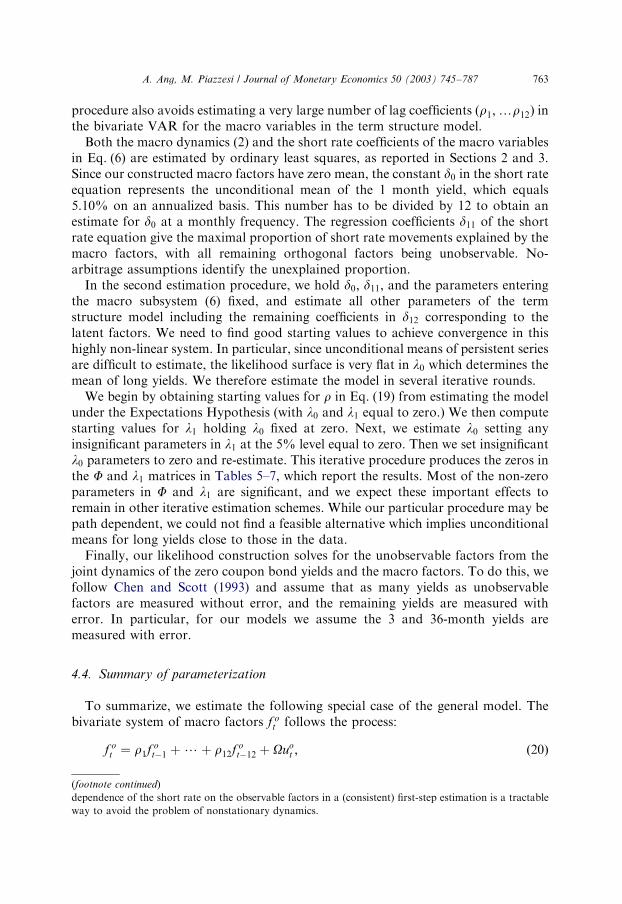


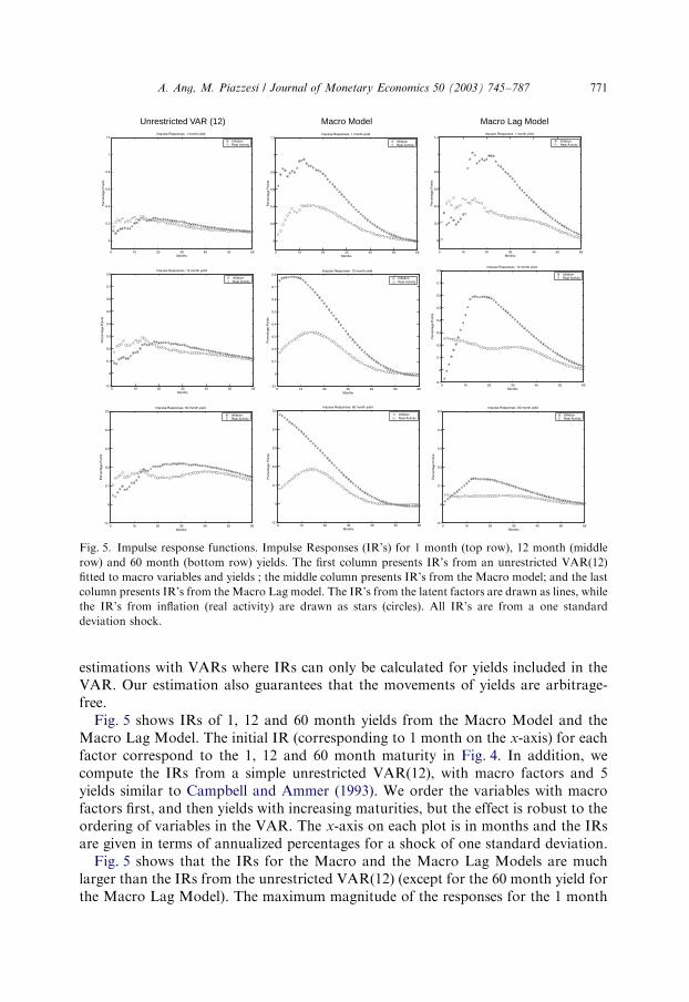


![23.Inflation - pdg.lbl.govpdg.lbl.gov/2017/reviews/rpp2017-rev-inflation.pdf · 23.Inflation 5 models [22,23,24], where inflation inside the bubble has a finite duration, leaving](https://static.documents.pub/doc/80x56/5e11caf48b6af83dd22a3107/23iniation-pdglbl-23iniation-5-models-222324-where-iniation-inside.jpg)
